Embed Size (px)
Citation preview
Computational Quantum Physics
Dr. Philippe de Forcrand ([email protected])and Prof. Matthias Troyer ([email protected])
ETH Zurich, SS 2008

Contents
1 Introduction 11.1 General . . . . . . . . . . . . . . . . . . . . . . . . . . . . . . . . . . . 1
1.1.1 Lecture Notes . . . . . . . . . . . . . . . . . . . . . . . . . . . . 11.1.2 Exercises . . . . . . . . . . . . . . . . . . . . . . . . . . . . . . . 11.1.3 Prerequisites . . . . . . . . . . . . . . . . . . . . . . . . . . . . . 21.1.4 References . . . . . . . . . . . . . . . . . . . . . . . . . . . . . . 2
1.2 Overview . . . . . . . . . . . . . . . . . . . . . . . . . . . . . . . . . . . 3
2 Quantum mechanics in one hour 42.1 Introduction . . . . . . . . . . . . . . . . . . . . . . . . . . . . . . . . . 42.2 Basis of quantum mechanics . . . . . . . . . . . . . . . . . . . . . . . . 4
2.2.1 Wave functions and Hilbert spaces . . . . . . . . . . . . . . . . 42.2.2 Mixed states and density matrices . . . . . . . . . . . . . . . . . 52.2.3 Observables . . . . . . . . . . . . . . . . . . . . . . . . . . . . . 52.2.4 The measurement process . . . . . . . . . . . . . . . . . . . . . 62.2.5 The uncertainty relation . . . . . . . . . . . . . . . . . . . . . . 72.2.6 The Schrodinger equation . . . . . . . . . . . . . . . . . . . . . 72.2.7 The thermal density matrix . . . . . . . . . . . . . . . . . . . . 8
2.3 The spin-S problem . . . . . . . . . . . . . . . . . . . . . . . . . . . . . 92.4 A quantum particle in free space . . . . . . . . . . . . . . . . . . . . . 9
2.4.1 The harmonic oscillator . . . . . . . . . . . . . . . . . . . . . . 10
3 The quantum one-body problem 123.1 The time-independent 1D Schrodinger equation . . . . . . . . . . . . . 12
3.1.1 The Numerov algorithm . . . . . . . . . . . . . . . . . . . . . . 123.1.2 The one-dimensional scattering problem . . . . . . . . . . . . . 133.1.3 Bound states and solution of the eigenvalue problem . . . . . . 14
3.2 The time-independent Schrodinger equation in higher dimensions . . . 153.2.1 Factorization along coordinate axis . . . . . . . . . . . . . . . . 153.2.2 Potential with spherical symmetry . . . . . . . . . . . . . . . . 163.2.3 Finite difference methods . . . . . . . . . . . . . . . . . . . . . . 163.2.4 Variational solutions using a finite basis set . . . . . . . . . . . 17
3.3 The time-dependent Schrodinger equation . . . . . . . . . . . . . . . . 183.3.1 Spectral methods . . . . . . . . . . . . . . . . . . . . . . . . . . 193.3.2 Direct numerical integration . . . . . . . . . . . . . . . . . . . . 193.3.3 The split operator method . . . . . . . . . . . . . . . . . . . . . 20
i
4 Introduction to many-body quantum mechanics 224.1 The complexity of the quantum many-body problem . . . . . . . . . . 224.2 Indistinguishable particles . . . . . . . . . . . . . . . . . . . . . . . . . 23
4.2.1 Bosons and fermions . . . . . . . . . . . . . . . . . . . . . . . . 234.2.2 The Fock space . . . . . . . . . . . . . . . . . . . . . . . . . . . 244.2.3 Creation and annihilation operators . . . . . . . . . . . . . . . . 254.2.4 Nonorthogonal basis sets . . . . . . . . . . . . . . . . . . . . . . 27
5 Path integrals and quantum Monte Carlo 285.1 Introduction . . . . . . . . . . . . . . . . . . . . . . . . . . . . . . . . . 285.2 Recall: Monte Carlo essentials . . . . . . . . . . . . . . . . . . . . . . . 285.3 Notation and general idea . . . . . . . . . . . . . . . . . . . . . . . . . 305.4 Expression for the Green’s function . . . . . . . . . . . . . . . . . . . . 305.5 Diffusion Monte Carlo . . . . . . . . . . . . . . . . . . . . . . . . . . . 32
5.5.1 Importance sampling . . . . . . . . . . . . . . . . . . . . . . . . 335.5.2 Fermionic systems . . . . . . . . . . . . . . . . . . . . . . . . . 345.5.3 Useful references . . . . . . . . . . . . . . . . . . . . . . . . . . 35
5.6 Path integral Monte Carlo . . . . . . . . . . . . . . . . . . . . . . . . . 355.6.1 Main idea . . . . . . . . . . . . . . . . . . . . . . . . . . . . . . 355.6.2 Finite temperature . . . . . . . . . . . . . . . . . . . . . . . . . 365.6.3 Observables . . . . . . . . . . . . . . . . . . . . . . . . . . . . . 385.6.4 Monte Carlo simulation . . . . . . . . . . . . . . . . . . . . . . 395.6.5 Useful references . . . . . . . . . . . . . . . . . . . . . . . . . . 40
6 Electronic structure of molecules and atoms 416.1 Introduction . . . . . . . . . . . . . . . . . . . . . . . . . . . . . . . . . 416.2 The electronic structure problem . . . . . . . . . . . . . . . . . . . . . 416.3 Basis functions . . . . . . . . . . . . . . . . . . . . . . . . . . . . . . . 42
6.3.1 The electron gas . . . . . . . . . . . . . . . . . . . . . . . . . . 426.3.2 Atoms and molecules . . . . . . . . . . . . . . . . . . . . . . . . 42
6.4 Pseudo-potentials . . . . . . . . . . . . . . . . . . . . . . . . . . . . . . 436.5 The Hartree Fock method . . . . . . . . . . . . . . . . . . . . . . . . . 44
6.5.1 The Hartree-Fock approximation . . . . . . . . . . . . . . . . . 446.5.2 The Hartree-Fock equations in nonorthogonal basis sets . . . . . 446.5.3 Configuration-Interaction . . . . . . . . . . . . . . . . . . . . . . 46
6.6 Density functional theory . . . . . . . . . . . . . . . . . . . . . . . . . . 466.6.1 Local Density Approximation . . . . . . . . . . . . . . . . . . . 486.6.2 Improved approximations . . . . . . . . . . . . . . . . . . . . . 48
6.7 Car-Parinello molecular dynamics . . . . . . . . . . . . . . . . . . . . . 486.8 Program packages . . . . . . . . . . . . . . . . . . . . . . . . . . . . . . 49
7 Exact diagonalization of the quantum many body problem 507.1 Models . . . . . . . . . . . . . . . . . . . . . . . . . . . . . . . . . . . . 50
7.1.1 The tight-binding model . . . . . . . . . . . . . . . . . . . . . . 507.1.2 The Hubbard model . . . . . . . . . . . . . . . . . . . . . . . . 517.1.3 The Heisenberg model . . . . . . . . . . . . . . . . . . . . . . . 51
ii
7.1.4 The t-J model . . . . . . . . . . . . . . . . . . . . . . . . . . . . 517.2 Exact diagonalization . . . . . . . . . . . . . . . . . . . . . . . . . . . . 51
8 Cluster quantum Monte Carlo algorithms for lattice models 568.1 World line representations for quantum lattice models . . . . . . . . . . 56
8.1.1 The stochastic series expansion (SSE) . . . . . . . . . . . . . . . 588.2 Cluster updates . . . . . . . . . . . . . . . . . . . . . . . . . . . . . . . 60
8.2.1 Kandel-Domany framework . . . . . . . . . . . . . . . . . . . . 608.2.2 The cluster algorithms for the Ising model . . . . . . . . . . . . 618.2.3 Improved Estimators . . . . . . . . . . . . . . . . . . . . . . . . 628.2.4 The loop algorithm for quantum spins . . . . . . . . . . . . . . 64
8.3 The negative sign problem . . . . . . . . . . . . . . . . . . . . . . . . . 698.4 Worm and directed loop updates . . . . . . . . . . . . . . . . . . . . . 72
9 An Introduction to Quantum Field Theory 739.1 Introduction . . . . . . . . . . . . . . . . . . . . . . . . . . . . . . . . . 739.2 Path integrals: from classical mechanics to field theory . . . . . . . . . 739.3 Numerical study of φ4 theory . . . . . . . . . . . . . . . . . . . . . . . 769.4 Gauge theories . . . . . . . . . . . . . . . . . . . . . . . . . . . . . . . 79
9.4.1 QED . . . . . . . . . . . . . . . . . . . . . . . . . . . . . . . . . 799.4.2 QCD . . . . . . . . . . . . . . . . . . . . . . . . . . . . . . . . . 81
9.5 Overview . . . . . . . . . . . . . . . . . . . . . . . . . . . . . . . . . . . 839.6 Useful references . . . . . . . . . . . . . . . . . . . . . . . . . . . . . . 84
A Numerical methods aA.1 Numerical root solvers . . . . . . . . . . . . . . . . . . . . . . . . . . . a
A.1.1 The Newton and secant methods . . . . . . . . . . . . . . . . . aA.1.2 The bisection method and regula falsi . . . . . . . . . . . . . . . bA.1.3 Optimizing a function . . . . . . . . . . . . . . . . . . . . . . . b
A.2 The Lanczos algorithm . . . . . . . . . . . . . . . . . . . . . . . . . . . c
iii
Chapter 1
Introduction
1.1 General
For physics students the computational quantum physics courses is a recommendedprerequisite for any computationally oriented semester thesis, proseminar, diploma the-sis or doctoral thesis.
For computational science and engineering (RW) students the computa-tional quantum physics courses is part of the “Vertiefung” in theoretical physics.
1.1.1 Lecture Notes
All the lecture notes, source codes, applets and supplementary material can be foundon our web page http://www.itp.phys.ethz.ch/lectures/CQP/.
1.1.2 Exercises
Programming Languages
Except when a specific programming language or tool is explicitly requested you arefree to choose any programming language you like. Solutions will often be given eitheras C++ programs or Mathematica Notebooks.
Computer Access
The lecture rooms offer both Linux workstations, for which accounts can be requestedwith the computer support group of the physics department in the HPR building, aswell as connections for your notebook computers.
1
1.1.3 Prerequisites
As a prerequisite for this course we expect knowledge of the following topics. Pleasecontact us if you have any doubts or questions.
Computing
• Basic knowledge of UNIX
• At least one procedural programming language such as C, C++, Pascal, Java orFORTRAN. C++ knowledge is preferred.
• Knowledge of a symbolic mathematics program such as Mathematica or Maple.
• Ability to produce graphical plots.
Numerical Analysis
• Numerical integration and differentiation
• Linear solvers and eigensolvers
• Root solvers and optimization
• Statistical analysis
Quantum Mechanics
Basic knowledge of quantum mechanics, at the level of the quantum mechanics taughtto computational scientists, should be sufficient to follow the course. If you feel lost atany point, please ask the lecturer to explain whatever you do not understand. We wantyou to be able to follow this course without taking an advanced quantum mechanicsclass.
1.1.4 References
1. J.M. Thijssen, Computational Physics, Cambridge University Press (1999) ISBN0521575885
2. Nicholas J. Giordano, Computational Physics, Pearson Education (1996) ISBN0133677230.
3. Harvey Gould and Jan Tobochnik, An Introduction to Computer Simulation Meth-ods, 2nd edition, Addison Wesley (1996), ISBN 00201506041
4. Tao Pang, An Introduction to Computational Physics, Cambridge University Press(1997) ISBN 0521485924
2
1.2 Overview
In this class we will learn how to simulate quantum systems, starting from the simpleone-dimensional Schrodinger equation to simulations of interacting quantum many bodyproblems in condensed matter physics and in quantum field theories. In particular wewill study
• The one-body Schrodinger equation and its numerical solution
• The many-body Schrodinger equation and second quantization
• Approximate solutions to the many body Schrodinger equation
• Path integrals and quantum Monte Carlo simulations
• Numerically exact solutions to (some) many body quantum problems
• Some simple quantum field theories
3
Chapter 2
Quantum mechanics in one hour
2.1 Introduction
The purpose of this chapter is to refresh your knowledge of quantum mechanics andto establish notation. Depending on your background you might not be familiar withall the material presented here. If that is the case, please ask the lecturers and wewill expand the introduction. Those students who are familiar with advanced quantummechanics are asked to glance over some omissions and are encouraged to help usimprove this quick introduction.
2.2 Basis of quantum mechanics
2.2.1 Wave functions and Hilbert spaces
Quantum mechanics is nothing but simple linear algebra, albeit in huge Hilbert spaces,which makes the problem hard. The foundations are pretty simple though.
A pure state of a quantum system is described by a “wave function” |Ψ〉, which isan element of a Hilbert space H:
|Ψ〉 ∈ H (2.1)
Usually the wave functions are normalized:
|| |Ψ〉 || =√
〈Ψ|Ψ〉 = 1. (2.2)
Here the “bra-ket” notation〈Φ|Ψ〉 (2.3)
denotes the scalar product of the two wave functions |Φ〉 and |Ψ〉.The simplest example is the spin-1/2 system, describing e.g. the two spin states
of an electron. Classically the spin ~S of the electron (which can be visualized as aninternal angular momentum), can point in any direction. In quantum mechanics it isdescribed by a two-dimensional complex Hilbert space H = C
2. A common choice of
4
basis vectors are the “up” and “down” spin states
| ↑〉 =
(
10
)
(2.4)
| ↓〉 =
(
01
)
(2.5)
This is similar to the classical Ising model, but in contrast to a classical Ising spinthat can point only either up or down, the quantum spin can exist in any complexsuperposition
|Ψ〉 = α| ↑〉+ β| ↓〉 (2.6)
of the basis states, where the normalization condition (2.2) requires that |α|2+ |β|2 = 1.For example, as we will see below the state
| →〉 =1√2
(| ↑〉+ | ↓〉) (2.7)
is a superposition that describes the spin pointing in the positive x-direction.
2.2.2 Mixed states and density matrices
Unless specifically prepared in a pure state in an experiment, quantum systems inNature rarely exist as pure states but instead as probabilistic superpositions. The mostgeneral state of a quantum system is then described as a density matrix ρ, with unittrace
Trρ = 1. (2.8)
The density matrix of a pure state is just the projector onto that state
ρpure = |Ψ〉〈Ψ|. (2.9)
For example, the density matrix of a spin pointing in the positive x-direction is
ρ→ = | →〉〈→ | =(
1/2 1/21/2 1/2
)
. (2.10)
Instead of being in a coherent superposition of up and down, the system could alsobe in a probabilistic mixed state, with a 50% probability of pointing up and a 50%probability of pointing down, which would be described by the density matrix
ρmixed =
(
1/2 00 1/2
)
. (2.11)
2.2.3 Observables
Any physical observable is represented by a self-adjoint linear operator acting on theHilbert space, which in a final dimensional Hilbert space can be represented by a Hermi-tian matrix. For our spin-1/2 system, using the basis introduced above, the components
5
Sx, Sy and Sz of the spin in the x-, y-, and z-directions are represented by the Paulimatrices
Sx =~
2σx =
~
2
(
0 11 0
)
(2.12)
Sy =~
2σy =
~
2
(
0 −ii 0
)
(2.13)
Sz =~
2σz =
~
2
(
1 00 −1
)
(2.14)
The spin component along an arbitrary unit vector e is the linear superposition ofthe components, i.e.
e · ~S = exSx + eySy + ezSz =~
2
(
ez ex − ieyex + iey −ez
)
(2.15)
The fact that these observables do not commute but instead satisfy the non-trivialcommutation relations
[Sx, Sy] = SxSy − SySx = i~Sz, (2.16)
[Sy, Sz] = i~Sx, (2.17)
[Sz, Sx] = i~Sy, (2.18)
will have important consequences.
2.2.4 The measurement process
The outcome of a measurement in a quantum system is usually intrusive and not deter-ministic. After measuring an observable A, the new wave function of the system will bean eigenvector of A and the outcome of the measurement the corresponding eigenvalue.The state of the system is thus changed by the measurement process!
For example, if we start with a spin pointing up with wave function
|Ψ〉 = | ↑〉 =
(
10
)
(2.19)
or alternatively density matrix
ρ↑ =
(
1 00 0
)
(2.20)
and we measure the x-component of the spin Sx, the resulting measurement will beeither +~/2 or −~/2, depending on whether the spin after the measurement points inthe + or − x-direction, and the wave function after the measurement will be either of
| →〉 =1√2
(| ↑〉+ | ↓〉) =
(
1/21/2
)
(2.21)
| ←〉 =1√2
(| ↑〉 − | ↓〉) =
(
1/2−1/2
)
(2.22)
6
Either of these states will be picked with a probability given by the overlap of the initialwave function by the individual eigenstates:
p→ = ||〈→ |Ψ〉||2 = 1/2 (2.23)
p← = ||〈← |Ψ〉||2 = 1/2 (2.24)
The final state is a probabilistic superposition of these two outcomes, described by thedensity matrix
ρ = p→| →〉〈→ |+ p←| ←〉〈← | =(
1/2 00 1/2
)
. (2.25)
which differs from the initial density matrix ρ↑.If we are not interested in the result of a particular outcome, but just in the average,
the expectation value of the measurement can easily be calculated from a wave function|Ψ〉 as
〈A〉 = 〈Ψ|A|Ψ〉 (2.26)
or from a density matrix ρ as〈A〉 = Tr(ρA). (2.27)
It is easy to convince yourself that for pure states the two formulations are identical.
2.2.5 The uncertainty relation
If two observables A and B do not commute [A,B] 6= 0, they cannot be measuredsimultaneously. If A is measured first, the wave function is changed to an eigenstate ofA, which changes the result of a subsequent measurement of B. As a consequence thevalues of A and B in a state Ψ cannot be simultaneously known, which is quantified bythe famous Heisenberg uncertainty relation which states that if two observables A andB do not commute but satisfy
[A,B] = i~ (2.28)
then the product of the root-mean-square deviations ∆A and ∆B of simultaneous mea-surements of A and B has to be larger than
∆A∆B ≥ ~/2 (2.29)
For more details about the uncertainty relation, the measurement process or the inter-pretation of quantum mechanics we refer interested students to an advanced quantummechanics class or text book.
2.2.6 The Schrodinger equation
The time-dependent Schrodinger equation
After so much introduction the Schrodinger equation is very easy to present. The wavefunction |Ψ〉 of a quantum system evolves according to
i~∂
∂t|Ψ(t)〉 = H|Ψ(t)〉, (2.30)
where H is the Hamilton operator. This is just a first order linear differential equation.
7
The time-independent Schrodinger equation
For a stationary time-independent problem the Schrodinger equation can be simplified.Using the ansatz
|Ψ(t)〉 = exp(−iEt/~)|Ψ〉, (2.31)
where E is the energy of the system, the Schrodinger equation simplifies to a lineareigenvalue problem
H|Ψ〉 = E|Ψ〉. (2.32)
The rest of the semester will be spent solving just this simple eigenvalue problem!
The Schrodinger equation for the density matrix
The time evolution of a density matrix ρ(t) can be derived from the time evolution ofpure states, and can be written as
i~∂
∂tρ(t) = [H, ρ(t)] (2.33)
The proof is left as a simple exercise.
2.2.7 The thermal density matrix
Finally we want to describe a physical system not in the ground state but in thermalequilibrium at a given inverse temperature β = 1/kBT . In a classical system each mi-crostate i of energy Ei is occupied with a probability given by the Boltzman distribution
pi =1
Zexp(−βEi), (2.34)
where the partition function
Z =∑
i
exp(−βEi) (2.35)
normalizes the probabilities.In a quantum system, if we use a basis of eigenstates |i〉 with energy Ei, the density
matrix can be written analogously as
ρβ =1
Z
∑
i
exp(−βEi)|i〉〈i| (2.36)
For a general basis, which is not necessarily an eigenbasis of the Hamiltonian H , thedensity matrix can be obtained by diagonalizing the Hamiltonian, using above equation,and transforming back to the original basis. The resulting density matrix is
ρβ =1
Zexp(−βH) (2.37)
where the partition function now is
Z = Tr exp(−βH) (2.38)
Calculating the thermal average of an observable A in a quantum system is hencevery easy:
〈A〉 = Tr(Aρβ) =TrA exp(−βH)
Tr exp(−βH). (2.39)
8
2.3 The spin-S problem
Before discussing solutions of the Schrodinger equation we will review two very simplesystems: a localized particle with general spin S and a free quantum particle.
In section 2.2.1 we have already seen the Hilbert space and the spin operators for themost common case of a spin-1/2 particle. The algebra of the spin operators given by thecommutation relations (2.12)-(2.12) allows not only the two-dimensional representationshown there, but a series of 2S + 1-dimensional representations in the Hilbert spaceC2S+1 for all integer and half-integer values S = 0, 1
2, 1, 3
2, 2, . . .. The basis states {|s〉}
are usually chosen as eigenstates of the Sz operator
Sz|s〉 = ~s|s〉, (2.40)
where s can take any value in the range −S,−S + 1,−S + 2, . . . , S− 1, S. In this basisthe Sz operator is diagonal, and the Sx and Sy operators can be constructed from the“ladder operators”
S+|s〉 =√
S(S + 1)− s(s+ 1)|s+ 1〉 (2.41)
S−|s〉 =√
S(S + 1)− s(s− 1)|s− 1〉 (2.42)
which increment or decrement the Sz value by 1 through
Sx =1
2
(
S+ + S−)
(2.43)
Sy =1
2i
(
S+ − S−)
. (2.44)
The Hamiltonian of the spin coupled to a magnetic field ~h is
H = −gµB~h · ~S, (2.45)
which introduces nontrivial dynamics since the components of ~S do not commute. Asa consequence the spin precesses around the magnetic field direction.
Exercise: Derive the differential equation governing the rotation of a spin startingalong the +x-direction rotating under a field in the +z-direction
2.4 A quantum particle in free space
Our second example is a single quantum particle in an n-dimensional free space. ItsHilbert space is given by all twice-continuously differentiable complex functions overthe real space Rn. The wave functions |Ψ〉 are complex-valued functions Ψ(~x) in n-dimensional space. In this representation the operator x, measuring the position of theparticle is simple and diagonal
x = ~x, (2.46)
while the momentum operator p becomes a differential operator
p = −i~∇. (2.47)
9
These two operators do not commute but their commutator is
[x, p] = i~. (2.48)
The Schrodinger equation of a quantum particle in an external potential V (~x) can beobtained from the classical Hamilton function by replacing the momentum and positionvariables by the operators above. Instead of the classical Hamilton function
H(~x, ~p) =~p2
2m+ V (~x) (2.49)
we use the quantum mechanical Hamiltonian operator
H =p2
2m+ V (x) = − ~
2
2m∇2 + V (~x), (2.50)
which gives the famous form
i~∂ψ
∂t= − ~2
2m∇2ψ + V (~x)ψ (2.51)
of the one-body Schrodinger equation.
2.4.1 The harmonic oscillator
As a special exactly solvable case let us consider the one-dimensional quantum harmonicoscillator with mass m and potential K
2x2. Defining momentum p and position operators
q in units where m = ~ = K = 1, the time-independent Schrodinger equation is givenby
H|n〉 = 1
2(p2 + q2)|n〉 = En|n〉 (2.52)
Inserting the definition of p we obtain an eigenvalue problem of an ordinary differentialequation
−1
2φ′′n(q) +
1
2q2φn(q) = Enφn(q) (2.53)
whose eigenvalues En = (n+ 1/2) and eigenfunctions
φn(q) =1
√
2nn!√π
exp
(
−1
2q2
)
Hn(q), (2.54)
are known analytically. Here the Hn are the Hermite polynomials and n = 0, 1, . . ..Using these eigenstates as a basis sets we need to find the representation of q and
p. Performing the integrals
〈m|q|n〉 and 〈m|p|n〉 (2.55)
it turns out that they are nonzero only for m = n± 1 and they can be written in termsof “ladder operators” a and a†:
q =1√2(a† + a) (2.56)
p =1
i√
2(a† − a) (2.57)
(2.58)
10
where the raising and lowering operators a† and a only have the following nonzeromatrix elements:
〈n+ 1|a†|n〉 = 〈n|a|n+ 1〉 =√n+ 1. (2.59)
and commutation relations
[a, a] = [a†, a†] = 0 (2.60)
[a, a†] = 1. (2.61)
It will also be useful to introduce the number operator n = a†a which is diagonal witheigenvalue n: elements
n|n〉 = a†a|n〉 =√na†|n− 1〉 = n||n〉. (2.62)
To check this representation let us plug the definitions back into the Hamiltonian toobtain
H =1
2(p2 + q2)
=1
4
[
−(a† − a)2 + (a† + a)2]
=1
2(a†a + aa†)
=1
2(2a†a + 1) = n +
1
2, (2.63)
which has the correct spectrum. In deriving the last lines we have used the commutationrelation (2.61).
11
Chapter 3
The quantum one-body problem
3.1 The time-independent 1D Schrodinger equation
We start the numerical solution of quantum problems with the time-indepent one-dimensional Schrodinger equation for a particle with mass m in a Potential V (x). Inone dimension the Schrodinger equation is just an ordinary differential equation
− ~2
2m
∂2ψ
∂x2+ V (x)ψ(x) = Eψ(x). (3.1)
We start with simple finite-difference schemes and discretize space into intervals oflength ∆x and denote the space points by
xn = n∆x (3.2)
and the wave function at these points by
ψn = ψ(xn). (3.3)
3.1.1 The Numerov algorithm
After rewriting the second order differential equation to a coupled system of two firstorder differential equations, any ODE solver such as the Runge-Kutta method could beapplied, but there exist better methods. For the special form
ψ′′(x) + k(x)ψ(x) = 0, (3.4)
of the Schrodinger equation, with k(x) = 2m(E−V (x))/~2 we can derive the Numerovalgorithm by starting from the Taylor expansion of ψn:
ψn±1 = ψn ±∆xψ′n +∆x2
2ψ′′n ±
∆x3
6ψ(3)n +
∆x4
24ψ(4)n ±
∆x5
120ψ(5)n + O(∆x6) (3.5)
Adding ψn+1 and ψn−1 we obtain
ψn+1 + ψn−1 = 2ψn + (∆x)2ψ′′n +(∆x)4
12ψ(4)n . (3.6)
12
Replacing the fourth derivatives by a finite difference second derivative of the secondderivatives
ψ(4)n =
ψ′′n+1 + ψ′′n−1 − 2ψ′′n∆x2
(3.7)
and substituting −k(x)ψ(x) for ψ′′(x) we obtain the Numerov algorithm
(
1 +(∆x)2
12kn+1
)
ψn+1 = 2
(
1− 5(∆x)2
12kn
)
ψn
−(
1 +(∆x)2
12kn−1
)
ψn−1 + O(∆x6), (3.8)
which is locally of sixth order!
Initial values
To start the Numerov algorithm we need the wave function not just at one but at twoinitial values and will now present several ways to obtain these.
For potentials V (x) with reflection symmetry V (x) = V (−x) the wave functionsneed to be either even ψ(x) = ψ(−x) or odd ψ(x) = −ψ(−x) under reflection, whichcan be used to find initial values:
• For the even solution we use a half-integer mesh with mesh points xn+1/2 =(n + 1/2)∆x and pick initial values ψ(x−1/2) = ψ(x1/2) = 1.
• For the odd solution we know that ψ(0) = −ψ(0) and hence ψ(0) = 0, specifyingthe first starting value. Using an integer mesh with mesh points xn = n∆x wepick ψ(x1) = 1 as the second starting value.
In general potentials we need to use other approaches. If the potentials vanishes forlarge distances: V (x) = 0 for |x| ≥ a we can use the exact solution of the Schrodingerequation at large distances to define starting points, e.g.
ψ(−a) = 1 (3.9)
ψ(−a−∆x) = exp(−∆x√
2mE/~). (3.10)
Finally, if the potential never vanishes we need to begin with a single starting valueψ(x0) and obtain the second starting value ψ(x1) by performing an integration over thefirst time step ∆τ with an Euler or Runge-Kutta algorithm.
3.1.2 The one-dimensional scattering problem
The scattering problem is the numerically easiest quantum problem since solutionsexist for all energies E > 0, if the potential vanishes at large distances (V (x) → 0 for|x| → ∞). The solution becomes particularly simple if the potential is nonzero onlyon a finite interval [0, a]. For a particle approaching the potential barrier from the left(x < 0) we can make the following ansatz for the free propagation when x < 0:
ψL(x) = A exp(−iqx) +B exp(iqx) (3.11)
13
where A is the amplitude of the incoming wave and B the amplitude of the reflectedwave. On the right hand side, once the particle has left the region of finite potential(x > a), we can again make a free propagation ansatz,
ψR(x) = C exp(−iqx) (3.12)
The coefficients A, B and C have to be determined self-consistently by matching to anumerical solution of the Schrodinger equation in the interval [0, a]. This is best donein the following way:
• Set C = 1 and use the two points a and a+ ∆x as starting points for a Numerovintegration.
• Integrate the Schrodinger equation numerically – backwards in space, from a to0 – using the Numerov algorithm.
• Match the numerical solution of the Schrodinger equation for x < 0 to the freepropagation ansatz (3.11) to determine A and B.
Once A and B have been determined the reflection and transmission probabilities Rand T are given by
R = |B|2/|A|2 (3.13)
T = 1/|A|2 (3.14)
3.1.3 Bound states and solution of the eigenvalue problem
While there exist scattering states for all energies E > 0, bound states solutions of theSchrodinger equation with E < 0 exist only for discrete energy eigenvalues. Integratingthe Schrodinger equation from −∞ to +∞ the solution will diverge to ±∞ as x→∞for almost all values. These functions cannot be normalized and thus do not constitutesolutions to the Schrodinger equation. Only for some special eigenvalues E, will thesolution go to zero as x→∞.
A simple eigensolver can be implemented using the following shooting method, wherewe again will assume that the potential is zero outside an interval [0, a]:
• Start with an initial guess E
• Integrate the Schrodinger equation for ψE(x) from x = 0 to xf ≫ a and determinethe value ψE(xf )
• use a root solver, such as a bisection method (see appendix A.1), to look for anenergy E with ψE(xf) ≈ 0
This algorithm is not ideal since the divergence of the wave function for x ± ∞ willcause roundoff error to proliferate.
A better solution is to integrate the Schrodinger equation from both sides towardsthe center:
• We search for a point b with V (b) = E
14
• Starting from x = 0 we integrate the left hand side solution ψL(x) to a chosen pointb and obtain ψL(b) and a numerical estimate for ψ′L(b) = (ψL(b)−ψL(b−∆x))/∆x.
• Starting from x = a we integrate the right hand solution ψR(x) down to the samepoint b and obtain ψR(b) and a numerical estimate for ψ′R(b) = (ψR(b + ∆x) −ψR(b))/∆x.
• At the point b the wave functions and their first two derivatives have to match,since solutions to the Schrodinger equation have to be twice continuously differen-tiable. Keeping in mind that we can multiply the wave functions by an arbitraryfactor we obtain the conditions
ψL(b) = αψR(b) (3.15)
ψ′L(b) = αψ′R(b) (3.16)
ψ′′L(b) = αψ′′R(b) (3.17)
The last condition is automatically fulfilled since by the choice V (b) = E theSchrodinger equation at b reduces to ψ′′(b) = 0. The first two conditions can becombined to the condition that the logarithmic derivatives vanish:
d logψLdx
|x=b =ψ′L(b)
ψL(b)=ψ′R(b)
ψR(b)=d logψRdx
|x=b (3.18)
• This last equation has to be solved for in a shooting method, e.g. using a bisectionalgorithm
Finally, at the end of the calculation, normalize the wave function.
3.2 The time-independent Schrodinger equation in
higher dimensions
The time independent Schrodinger equation in more than one dimension is a partialdifferential equation and cannot, in general, be solved by a simple ODE solver such asthe Numerov algorithm. Before employing a PDE solver we should thus always first tryto reduce the problem to a one-dimensional problem. This can be done if the problemfactorizes.
3.2.1 Factorization along coordinate axis
A first example is a three-dimensional Schrodinger equation in a cubic box with potentialV (~r) = V (x)V (y)V (z) with ~r = (x, y, z). Using the product ansatz
ψ(~r) = ψx(x)ψy(y)ψz(z) (3.19)
the PDE factorizes into three ODEs which can be solved as above.
15
3.2.2 Potential with spherical symmetry
Another famous trick is possible for spherically symmetric potentials with V (~r) = V (|~r|)where an ansatz using spherical harmonics
ψl,m(~r) = ψl,m(r, θ, φ) =u(r)
rYlm(θ, φ) (3.20)
can be used to reduce the three-dimensional Schrodinger equation to a one-dimensionalone for the radial wave function u(r):
[
− ~2
2m
d2
dr2+
~2l(l + 1)
2mr2+ V (r)
]
u(r) = Eu(r) (3.21)
in the interval [0,∞[. Given the singular character of the potential for r → 0, anumerical integration should start at large distances r and integrate towards r = 0, sothat the largest errors are accumulated only at the last steps of the integration.
3.2.3 Finite difference methods
The simplest solvers for partial differential equations, the finite difference solvers canalso be used for the Schrodinger equation. Replacing differentials by differences weconvert the Schrodinger equation to a system of coupled inear equations. Starting fromthe three-dimensional Schrodinger equation (we set ~ = 1 from now on)
∇2ψ(~x) + 2m(V − E(~x))ψ(~x) = 0, (3.22)
we discretize space and obtain the system of linear equations
1
∆x2[ψ(xn+1, yn, zn) + ψ(xn−1, yn, zn)
+ψ(xn, yn+1, zn) + ψ(xn, yn−1, zn) (3.23)
+ψ(xn, yn, zn+1) + ψ(xn, yn, zn−1)]
+
[
2m(V (~x)− E)− 6
∆x2
]
ψ(xn, yn, zn) = 0.
For the scattering problem a linear equation solver can now be used to solve thesystem of equations. For small linear problems Mathematica can be used, or the dsysv
function of the LAPACK library. For larger problems it is essential to realize that thematrices produced by the discretization of the Schrodinger equation are usually verysparse, meaning that only O(N) of the N2 matrix elements are nonzero. For thesesparse systems of equations, optimized iterative numerical algorithms exist1 and areimplemented in numerical libraries such as in the ITL library.2
1R. Barret, M. Berry, T.F. Chan, J. Demmel, J. Donato, J. Dongarra, V. Eijkhout, R. Pozo, C.Romine, and H. van der Vorst, Templates for the Solution of Linear Systems: Building Blocks forIterative Methods (SIAM, 1993)
2J.G. Siek, A. Lumsdaine and Lie-Quan Lee, Generic Programming for High Performance NumericalLinear Algebra in Proceedings of the SIAM Workshop on Object Oriented Methods for Inter-operableScientific and Engineering Computing (OO’98) (SIAM, 1998); the library is availavle on the web at:http://www.osl.iu.edu/research/itl/
16
To calculate bound states, an eigenvalue problem has to be solved. For small prob-lems, where the full matrix can be stored in memory, Mathematica or the dsyev eigen-solver in the LAPACK library can be used. For bigger systems, sparse solvers such asthe Lanczos algorithm (see appendix A.2) are best. Again there exist efficient imple-mentations3 of iterative algorithms for sparse matrices.4
3.2.4 Variational solutions using a finite basis set
In the case of general potentials, or for more than two particles, it will not be possible toreduce the Schrodinger equation to a one-dimensional problem and we need to employa PDE solver. One approach will again be to discretize the Schrodinger equation on adiscrete mesh using a finite difference approximation. A better solution is to expandthe wave functions in terms of a finite set of basis functions
|φ〉 =N∑
i=1
ai|ui〉. (3.24)
To estimate the ground state energy we want to minimize the energy of the varia-tional wave function
E∗ =〈φ|H|φ〉〈φ|φ〉 . (3.25)
Keep in mind that, since we only chose a finite basis set {|ui〉} the variational estimateE∗ will always be larger than the true ground state energy E0, but will converge towardsE0 as the size of the basis set is increased, e.g. by reducing the mesh size in a finiteelement basis.
To perform the minimization we denote by
Hij = 〈ui|H|uj〉 =
∫
d~rui(~r)∗(
− ~2
2m∇2 + V
)
uj(~r) (3.26)
the matrix elements of the Hamilton operator H and by
Sij = 〈ui|uj〉 =
∫
d~rui(~r)∗uj(~r) (3.27)
the overlap matrix. Note that for an orthogonal basis set, Sij is the identity matrix δij .Minimizing equation (3.25) we obtain a generalized eigenvalue problem
∑
j
Hijaj = E∑
k
Sikak. (3.28)
or in a compact notation with ~a = (a1, . . . , aN)
H~a = ES~a. (3.29)
3http://www.comp-phys.org/software/ietl/4Z. Bai, J. Demmel and J. Dongarra (Eds.), Templates for the Solution of Algebraic Eigenvalue
Problems: A Practical Guide (SIAM, 2000).
17
If the basis set is orthogonal this reduces to an ordinary eigenvalue problem and we canuse the Lanczos algorithm.
In the general case we have to find orthogonal matrices U such that UTSU is theidentity matrix. Introducing a new vector~b = U−1~a. we can then rearrange the probleminto
H~a = ES~a
HU~b = ESU~b
UTHU~b = EUTSU~b = E~b (3.30)
and we end up with a standard eigenvalue problem for UTHU . Mathematica andLAPACK both contain eigensolvers for such generalized eigenvalue problems.
Example: the anharmonic oscillator
The final issue is the choice of basis functions. It is advantageous to make use of knownsolutions to a similar problem as we will illustrate in the case of an anharmonic oscillatorwith Hamilton operator
H = H0 + λq4
H0 =1
2(p2 + q2), (3.31)
where the harmonic oscillator H0 was already discussed in section 2.4.1. It makes senseto use the N lowest harmonic oscillator eigenvectors |n〉 as basis states of a finite basisand write the Hamiltonian as
H =1
2+ n + λq4 =
1
2+ n+
λ
4(a† + a)4 (3.32)
Since the operators a and a† are nonzero only in the first sub or superdiagonal, theresulting matrix is a banded matrix of bandwidth 9. A sparse eigensolver such as theLanczos algorithm can again be used to calculate the spectrum. Note that since weuse the orthonormal eigenstates of H0 as basis elements, the overlap matrix S here isthe identity matrix and we have to deal only with a standard eigenvalue problem. Asolution to this problem is provided in a Mathematica notebook on the web page.
The finite element method
In cases where we have irregular geometries or want higher precision than the lowestorder finite difference method, and do not know a suitable set of basis function, thefinite element method (FEM) should be chosen over the finite difference method. Sinceexplaining the FEM can take a full semester in itself, we refer interested students toclasses on solving partial differential equations.
3.3 The time-dependent Schrodinger equation
Finally we will reintroduce the time dependence to study dynamics in non-stationaryquantum systems.
18
3.3.1 Spectral methods
By introducing a basis and solving for the complete spectrum of energy eigenstates wecan directly solve the time-dependent problem in the case of a stationary Hamiltonian.This is a consequence of the linearity of the Schrodinger equation.
To calculate the time evolution of a state |ψ(t0)〉 from time t0 to t we first solvethe stationary eigenvalue problem H|φ〉 = E|φ〉 and calculate the eigenvectors |φn〉 andeigenvalues ǫn. Next we represent the initial wave function |ψ〉 by a spectral decompo-sition
|ψ(t0)〉 =∑
n
cn|φn〉. (3.33)
Since each of the |φn〉 is an eigenvector of H , the time evolution e−i~H(t−t0) is trivialand we obtain at time t:
|ψ(t)〉 =∑
n
cne−i~ǫn(t−t0)|φn〉. (3.34)
3.3.2 Direct numerical integration
If the number of basis states is too large to perform a complete diagonalization ofthe Hamiltonian, or if the Hamiltonian changes over time we need to perform a directintegration of the Schrodinger equation. Like other initial value problems of partialdifferential equations the Schrodinger equation can be solved by the method of lines.After choosing a set of basis functions or discretizing the spatial derivatives we obtain aset of coupled ordinary differential equations which can be evolved for each point alongthe time line (hence the name) by standard ODE solvers.
In the remainder of this chapter we use the symbol H to refer the representation ofthe Hamiltonian in the chosen finite basis set. A forward Euler scheme
|ψ(tn+1)〉 = |ψ(tn)〉 − i~∆tH|ψ(tn)〉 (3.35)
is not only numerically unstable. It also violates the conservation of the norm of thewave function 〈ψ|ψ〉 = 1. Since the exact quantum evolution
ψ(x, t+ ∆t) = e−i~H∆tψ(x, t). (3.36)
is unitary and thus conserves the norm, we want to look for a unitary approximant asintegrator. Instead of using the forward Euler method (3.35) which is just a first orderTaylor expansion of the exact time evolution
e−i~H∆t = 1− i~H∆t + O(∆2t ), (3.37)
we reformulate the time evolution operator as
e−i~H∆t =(
ei~H∆t/2)−1
e−i~H∆t/2 =
(
1 + i~H∆t
2
)−1(
1− i~H∆t
2
)
+ O(∆3t ), (3.38)
which is unitary!
19
This gives the simplest stable and unitary integrator algorithm
ψ(x, t+ ∆t) =
(
1 + i~H∆t
2
)−1(
1− i~H∆t
2
)
ψ(x, t) (3.39)
or equivalently
(
1 + i~H∆t
2
)
ψ(x, t+ ∆t) =
(
1− i~H∆t
2
)
ψ(x, t). (3.40)
Unfortunately this is an implicit integrator. At each time step, after evaluating theright hand side a linear system of equations needs to be solved. For one-dimensionalproblems the matrix representation of H is often tridiagonal and a tridiagonal solvercan be used. In higher dimensions the matrix H will no longer be simply tridiagonalbut still very sparse and we can use iterative algorithms, similar to the Lanczos algo-rithm for the eigenvalue problem. For details about these algorithms we refer to thenice summary at http://mathworld.wolfram.com/topics/Templates.html and es-pecially the biconjugate gradient (BiCG) algorithm. Implementations of this algorithmare available, e.g. in the Iterative Template Library (ITL).
3.3.3 The split operator method
A simpler and explicit method is possible for a quantum particle in the real space picturewith the “standard” Schrodinger equation (2.51). Writing the Hamilton operator as
H = T + V (3.41)
with
T =1
2mp2 (3.42)
V = V (~x) (3.43)
it is easy to see that V is diagonal in position space while T is diagonal in momentumspace. If we split the time evolution as
e−i~∆tH = e−i~∆tV /2e−i~∆tT e−i~∆tV /2 + O(∆3t ) (3.44)
we can perform the individual time evolutions e−i~∆tV /2 and e−i~∆tT exactly:
[
e−i~∆tV /2|ψ〉]
(~x) = e−i~∆tV (~x)/2ψ(~x) (3.45)[
e−i~∆tT /2|ψ〉]
(~k) = e−i~∆t||~k||2/2mψ(~k) (3.46)
in real space for the first term and momentum space for the second term. This requiresa basis change from real to momentum space, which is efficiently performed using a FastFourier Transform (FFT) algorithm. Propagating for a time t = N∆t, two consecutive
20
applications of e−i~∆tV /2 can easily be combined into a propagation by a full time stepe−i~∆tV , resulting in the propagation:
e−i~∆tH =(
e−i~∆tV /2e−i~∆tT e−i~∆tV /2)N
+ O(∆2t )
= e−i~∆tV /2[
e−i~∆tT e−i~∆tV]N−1
e−i~∆tT e−i~∆tV /2 (3.47)
and the discretized algorithm starts as
ψ1(~x) = e−i~∆tV (~x)/2ψ0(~x) (3.48)
ψ1(~k) = Fψ1(~x) (3.49)
where F denotes the Fourier transform and F−1 will denote the inverse Fourier trans-form. Next we propagate in time using full time steps:
ψ2n(~k) = e−i~∆t||~k||2/2mψ2n−1(~k) (3.50)
ψ2n(~x) = F−1ψ2n(~k) (3.51)
ψ2n+1(~x) = e−i~∆tV (~x)ψ2n(~x) (3.52)
ψ2n+1(~k) = Fψ2n+1(~x) (3.53)
except that in the last step we finish with another half time step in real space:
ψ2N+1(~x) = e−i~∆tV (~x)/2ψ2N (~x) (3.54)
This is a fast and unitary integrator for the Schrodinger equation in real space. It couldbe improved by replacing the locally third order splitting (3.44) by a fifth-order versioninvolving five instead of three terms.
21
Chapter 4
Introduction to many-bodyquantum mechanics
4.1 The complexity of the quantum many-body prob-
lem
After learning how to solve the 1-body Schrodinger equation, let us next generalize tomore particles. If a single body quantum problem is described by a Hilbert space Hof dimension dimH = d then N distinguishable quantum particles are described by thetensor product of N Hilbert spaces
H(N) ≡ H⊗N ≡N⊗
i=1
H (4.1)
with dimension dN .As a first example, a single spin-1/2 has a Hilbert space H = C2 of dimension 2,
but N spin-1/2 have a Hilbert space H(N) = C2N
of dimension 2N . Similarly, a singleparticle in three dimensional space is described by a complex-valued wave function ψ(~x)of the position ~x of the particle, while N distinguishable particles are described by acomplex-valued wave function ψ(~x1, . . . , ~xN ) of the positions ~x1, . . . , ~xN of the particles.Approximating the Hilbert space H of the single particle by a finite basis set with dbasis functions, the N -particle basis approximated by the same finite basis set for singleparticles needs dN basis functions.
This exponential scaling of the Hilbert space dimension with the number of particlesis a big challenge. Even in the simplest case – a spin-1/2 with d = 2, the basis forN = 30spins is already of of size 230 ≈ 109. A single complex vector needs 16 GByte of memoryand will not fit into the memory of your PC anymore.
22
This challenge will be to addressed later in this course by learning about
1. approximative methods, reducing the many-particle problem to a single-particleproblem
2. quantum Monte Carlo methods for bosonic and magnetic systems
3. brute-force methods solving the exact problem in a huge Hilbert space for modestnumbers of particles
4.2 Indistinguishable particles
4.2.1 Bosons and fermions
In quantum mechanics we assume that elementary particles, such as the electron orphoton, are indistinguishable: there is no serial number painted on the electrons thatwould allow us to distinguish two electrons. Hence, if we exchange two particles thesystem is still the same as before. For a two-body wave function ψ(~q1, ~q2) this meansthat
ψ(~q2, ~q1) = eiφψ(~q1, ~q2), (4.2)
since upon exchanging the two particles the wave function needs to be identical, up toa phase factor eiφ. In three dimensions the first homotopy group is trivial and afterdoing two exchanges we need to be back at the original wave function1
ψ(~q1, ~q2) = eiφψ(~q2, ~q1) = e2iφψ(~q1, ~q2), (4.3)
and hence e2iφ = ±1:ψ(~q2, ~q1) = ±ψ(~q1, ~q2) (4.4)
The many-body Hilbert space can thus be split into orthogonal subspaces, one in whichparticles pick up a − sign and are called fermions, and the other where particles pickup a + sign and are called bosons.
Bosons
For bosons the general many-body wave function thus needs to be symmetric underpermutations. Instead of an arbitrary wave function ψ(~q1, . . . , ~qN) of N particles weuse the symmetrized wave function
Ψ(S) = S+ψ(~q1, . . . , ~qN) ≡ NS∑
p
ψ(~qp(1), . . . , ~qp(N)), (4.5)
where the sum goes over all permutations p of N particles, and NS is a normalizationfactor.
1As a side remark we want to mention that in two dimensions the first homotopy group is Z and nottrivial: it matters whether we move the particles clock-wise or anti-clock wise when exchanging them,and two clock-wise exchanges are not the identity anymore. Then more general, anyonic, statistics arepossible.
23
Fermions
For fermions the wave function has to be antisymmetric under exchange of any twofermions, and we use the anti-symmetrized wave function
Ψ(A)S−ψ(~q1, . . . , ~qN) ≡ NA∑
p
sgn(p)ψ(~qp(1), . . . , ~qp(N)), (4.6)
where sgn(p) = ±1 is the sign of the permutation and NA again a normalization factor.A consequence of the antisymmetrization is that no two fermions can be in the same
state as a wave functionψ(~q1, ~q2) = φ(~q1)φ(~q2) (4.7)
since this vanishes under antisymmetrization:
Ψ(~q1, ~q2) = ψ(~q1, ~q2)− ψ(~q2, ~q1) = φ(~q1)φ(~q2)− φ(~q2)φ(~q1) = 0 (4.8)
Spinful fermions
Fermions, such as electrons, usually have a spin-1/2 degree of freedom in additionto their orbital wave function. The full wave function as a function of a generalizedcoordinate ~x = (~q, σ) including both position ~q and spin σ.
4.2.2 The Fock space
The Hilbert space describing a quantum many-body system with N = 0, 1, . . . ,∞particles is called the Fock space. It is the direct sum of the appropriately symmetrizedsingle-particle Hilbert spaces H:
∞⊕
N=0
S±H⊗n (4.9)
where S+ is the symmetrization operator used for bosons and S− is the anti-symmetrizationoperator used for fermions.
The occupation number basis
Given a basis {|φ1〉, . . . , |φL〉} of the single-particle Hilbert space H, a basis for theFock space is constructed by specifying the number of particles ni occupying the single-particle wave function |f1〉. The wave function of the state |n1, . . . , nL〉 is given by theappropriately symmetrized and normalized product of the single particle wave functions.For example, the basis state |1, 1〉 has wave function
1√2
[φ1(~x1)φ2(~x2)± φ1(~x2)φ2(~x1)] (4.10)
where the + sign is for bosons and the − sign for fermions.For bosons the occupation numbers ni can go from 0 to ∞, but for fermions they
are restricted to ni = 0 or 1 since no two fermions can occupy the same state.
24
The Slater determinant
The antisymmetrized and normalized product of N single-particle wave functions φican be written as a determinant, called the Slater determinant
S−N∏
i1
φi(~xi) =1√N
∣
∣
∣
∣
∣
∣
∣
φ1(~x1) · · · φN(~x1)...
...φ1(~xN) · · · φN(~xN )
∣
∣
∣
∣
∣
∣
∣
. (4.11)
Note that while the set of Slater determinants of single particle basis functions formsa basis of the fermionic Fock space, the general fermionic many body wave function is alinear superposition of many Slater determinants and cannot be written as a single Slaterdeterminant. The Hartee Fock method, discussed below, will simplify the quantummany body problem to a one body problem by making the approximation that theground state wave function can be described by a single Slater determinant.
4.2.3 Creation and annihilation operators
Since it is very cumbersome to work with appropriately symmetrized many body wavefunctions, we will mainly use the formalism of second quantization and work withcreation and annihilation operators.
The annihilation operator ai,σ associated with a basis function |φi〉 is defined as theresult of the inner product of a many body wave function |Ψ〉 with this basis function|φi〉. Given an N -particle wave function |Ψ(N)〉 the result of applying the annihilationoperator is an N − 1-particle wave function |Ψ(N)〉 = ai|Ψ(N)〉. It is given by theappropriately symmetrized inner product
Ψ(~x1, . . . , ~xN−1) = S±∫
d~xNf†i (~xN )Ψ(~x1, . . . , ~xN). (4.12)
Applied to a single-particle basis state |φj〉 the result is
ai|φj〉 = δij |0〉 (4.13)
where |0〉 is the “vacuum” state with no particles.The creation operator a†i is defined as the adjoint of the annihilation operator ai.
Applying it to the vacuum “creates” a particle with wave function φi:
|φi〉 = a†i |0〉 (4.14)
For sake of simplicity and concreteness we will now assume that the L basis functions|φi〉 of the single particle Hilbert space factor into L/(2S + 1) orbital wave functionsfi(~q) and 2S + 1 spin wave functions |σ〉, where σ = −S,−S + 1, ..., S. We will writecreation and annihilation operators a†i,σ and ai,σ where i is the orbital index and σ thespin index. The most common cases will be spinless bosons with S = 0, where the spinindex can be dropped and spin-1/2 fermions, where the spin can be up (+1/2) or down(−1/2).
25
Commutation relations
The creation and annihilation operators fulfill certain canonical commutation relations,which we will first discuss for an orthogonal set of basis functions. We will later gener-alize them to non-orthogonal basis sets.
For bosons, the commutation relations are the same as that of the ladder operatorsdiscussed for the harmonic oscillator (2.61):
[ai, aj ] = [a†i , a†j] = 0 (4.15)
[ai, a†j] = δij . (4.16)
For fermions, on the other hand, the operators anticommute
{a†jσ′ , aiσ} = {a†iσ, ajσ′} = δσσ′δij
{aiσ, ajσ′} = {a†iσ, a†jσ′} = 0. (4.17)
The anti-commutation implies that
(a†i )2 = a†ia
†i = −a†ia†i (4.18)
and that thus(a†i)
2 = 0, (4.19)
as expected since no two fermions can exist in the same state.
Fock basis in second quantization and normal ordering
The basis state |n1, . . . , nL〉 in the occupation number basis can easily be expressed interms of creation operators:
|n1, . . . , nL〉 =
L∏
i=1
(a†i )ni|0〉 = (a†1)
n1(a†2)n2 · · · (a†L)nL |0〉 (4.20)
For bosons the ordering of the creation operators does not matter, since the operatorscommute. For fermions, however, the ordering matters since the fermionic creationoperators anticommute: and a†1a
†2|0〉 = −a†1a†2|0〉. We thus need to agree on a specific
ordering of the creation operators to define what we mean by the state |n1, . . . , nL〉.The choice of ordering does not matter but we have to stay consistent and use e.g. theconvention in equation (4.20).
Once the normal ordering is defined, we can derive the expressions for the matrixelements of the creation and annihilation operators in that basis. Using above normalordering the matrix elements are
ai|n1, . . . , ni, . . . , nL〉 = δni,1(−1)Pi−1
j=1ni |n1, . . . , ni − 1, . . . , nL〉 (4.21)
a†i |n1, . . . , ni, . . . , nL〉 = δni,0(−1)Pi−1
j=1ni |n1, . . . , ni + 1, . . . , nL〉 (4.22)
where the minus signs come from commuting the annihilation and creation operator tothe correct position in the normal ordered product.
26
4.2.4 Nonorthogonal basis sets
In simulating the electronic properties of atoms and molecules below we will see thatthe natural choice of single particle basis functions centered around atoms will nec-essarily give a non-orthogonal set of basis functions. This is no problem, as long asthe definition of the annihilation and creation operators is carefully generalized. Forthis generalization it will be useful to introduce the fermion field operators ψ†σ(~r) andψσ(~r), creating and annihilating a fermion localized at a single point ~r in space. Theircommutation relations are simply
{ψ†σ′(~r), ψσ(~r′)} = {ψ†σ(~r), ψσ′(~r′)} = δσσ′δ(~r − ~r′){ψσ(~r), ψσ′(~r′)} = {ψ†σ(~r), ψ†σ′(~r′)} = 0. (4.23)
The scalar products of the basis functions define a matrix
Sij =
∫
d3~rf ∗i (~r)fj(~r), (4.24)
which is in general not the identity matrix. The associated annihilation operators aiσare again defined as scalar products
aiσ =∑
j
(S−1)ij
∫
d3~rf ∗j (~r)ψσ(~r). (4.25)
The non-orthogonality causes the commutation relations of these operators to differfrom those of normal fermion creation- and annihilation operators:
{a†iσ, ajσ′} = δσσ′(S−1)ij
{aiσ, ajσ′} = {a†iσ, a†jσ′} = 0. (4.26)
Due to the non-orthogonality the adjoint a†iσ does not create a state with wave functionfi. This is done by the operator a†iσ, defined through:
a†iσ =∑
j
Sjia†iσ, (4.27)
which has the following simple commutation relation with ajσ:
{a†iσ, ajσ} = δij . (4.28)
The commutation relations of the a†iσ and the ajσ′ are:
{a†iσajσ′} = δσσ′Sij
{aiσ, ajσ′} = {a†iσ, a†jσ′} = 0. (4.29)
We will need to keep the distinction between a and a in mind when dealing withnon-orthogonal basis sets.
27
Chapter 5
Path integrals and quantum MonteCarlo
5.1 Introduction
In this chapter, we continue the numerical study of a quantum many-body system. Thesystem is described by its wave-function ψ(~r1, ~r2, .., ~rN), which is a mapping RN → C.Finding the exact wave-function is not practically feasible unless N is very small. Theprevious chapter used a spectral approach, i.e. decomposed the wave-function ontoa carefully chosen set of basis functions, and found the best approximate solution ofthe Schrodinger equation in the corresponding vector space. In this chapter, we use thetechnique of Monte Carlo to obtain a noisy but unbiased estimator of the wave-function.This strategy goes by the general name of Quantum Monte Carlo, which covers manyvariants. I will describe the two main ones, called Diffusion Monte Carlo (or Green’sfunction Monte Carlo) and Path integral Monte Carlo. Diffusion Monte Carlo hasdeveloped into a precise tool to compute the groundstate properties of systems withO(103) particles. Path integral Monte Carlo is technically similar, but gives finite-temperature properties. The path integral formalism carries over to the relativisticcase, and forms an essential basis for the study of quantum field theory (to be reviewedin Chapter 8). Although some familiarity with Monte Carlo algorithms is desirable, thenecessary basic facts about Monte Carlo are summarized in the first section.
5.2 Recall: Monte Carlo essentials
• Monte Carlo is a powerful stochastic technique to estimate ratios of high-dimensionalintegrals.- Simple example: how much is π ? See Fig.5.1.
28
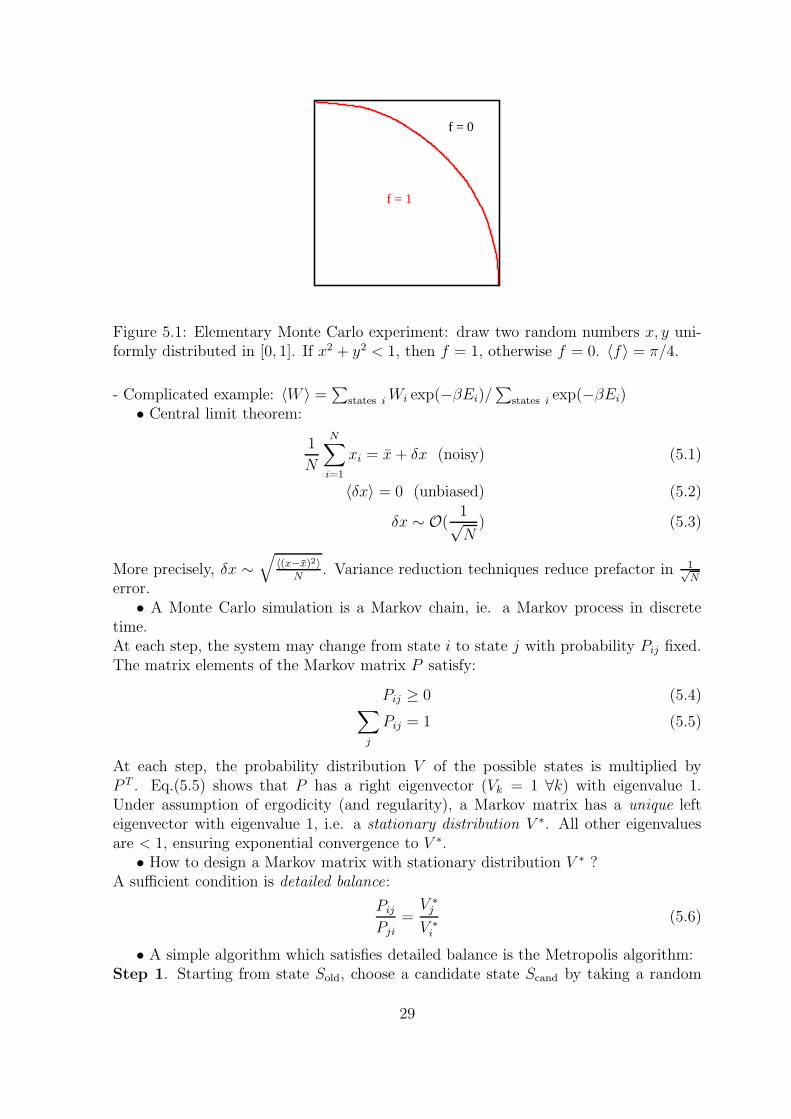
f = 1
f = 0
Figure 5.1: Elementary Monte Carlo experiment: draw two random numbers x, y uni-formly distributed in [0, 1]. If x2 + y2 < 1, then f = 1, otherwise f = 0. 〈f〉 = π/4.
- Complicated example: 〈W 〉 =∑
states iWi exp(−βEi)/∑
states i exp(−βEi)• Central limit theorem:
1
N
N∑
i=1
xi = x+ δx (noisy) (5.1)
〈δx〉 = 0 (unbiased) (5.2)
δx ∼ O(1√N
) (5.3)
More precisely, δx ∼√
〈(x−x)2〉N
. Variance reduction techniques reduce prefactor in 1√N
error.• A Monte Carlo simulation is a Markov chain, ie. a Markov process in discrete
time.At each step, the system may change from state i to state j with probability Pij fixed.The matrix elements of the Markov matrix P satisfy:
Pij ≥ 0 (5.4)∑
j
Pij = 1 (5.5)
At each step, the probability distribution V of the possible states is multiplied byP T . Eq.(5.5) shows that P has a right eigenvector (Vk = 1 ∀k) with eigenvalue 1.Under assumption of ergodicity (and regularity), a Markov matrix has a unique lefteigenvector with eigenvalue 1, i.e. a stationary distribution V ∗. All other eigenvaluesare < 1, ensuring exponential convergence to V ∗.• How to design a Markov matrix with stationary distribution V ∗ ?
A sufficient condition is detailed balance:
PijPji
=V ∗jV ∗i
(5.6)
• A simple algorithm which satisfies detailed balance is the Metropolis algorithm:Step 1. Starting from state Sold, choose a candidate state Scand by taking a random
29
step: Scand = R ◦ Sold, drawn from an even distribution: Prob(R−1) = Prob(R).Step 2. Accept the candidate state Scand as the next state Snew in the Markov chainwith probability
Prob(Snew = Scand) = min(1, V ∗(Scand)/V∗(Sold)) (5.7)
If Scand is rejected, set Snew = Sold in the Markov chain.
5.3 Notation and general idea
For simplicity of notation, I consider a single particle in one dimension. The wave-function ψ(x, t) is a mapping R ×R → C. The ket |ψ(t)〉 =
∫
dxψ(x, t)|x〉 is a statevector in the Hilbert space. |x〉 is an eigenstate of the position operator X: X|x〉 = x|x〉,with the completeness relation
∫
dx|x〉〈x| = 1.The time-dependent Schrodinger equation i~ d
dt|ψ〉 = H|ψ〉 has for solution
|ψ(t)〉 = exp(− i~Ht)|ψ(0)〉 (5.8)
Now change the time to pure imaginary, τ = it (also called performing a Wick rotationto Euclidean time), so that
|ψ(τ)〉 = exp(−τ~H)|ψ(0)〉 (5.9)
and expand in eigenstates of H : H|ψk〉 = Ek|ψk〉, k = 0, 1, .., E0 ≤ E1 ≤ ...
|ψ(τ)〉 =∑
k
exp(−τ~Ek)〈ψk|ψ(0)〉|ψk〉 (5.10)
It is apparent that τ~
acts as an inverse temperature, and that |ψ(τ)〉 will becomeproportional to the groundstate |ψ0〉 as τ → +∞, provided |ψ(0)〉 is not orthogonal toit. Diffusion and path integral Monte Carlo both simulate an imaginary time evolutionto obtain information on low-energy states.
Moreover, in both approaches, the time evolution is performed as a sum over histo-ries, each history having a different probability. Note that the same description is usedfor financial predictions, so you might learn something really useful here...
5.4 Expression for the Green’s function
As a starting point, notice that the Schrodinger equation is linear, so that its solution|ψ(t)〉 = exp(− i
~Ht)|ψ(0)〉 is equivalent to
ψ(x, t) =
∫
dx0G(x, t; x0, 0)ψ(x0, 0) (5.11)
where
G(x, t; x0, 0) ≡ 〈x| exp(− i~Ht)|x0〉 (5.12)
30
is the Green’s function, i.e. the solution of the Schrodinger equation for ψ(x, 0) =δ(x− x0) (also called transition amplitude, or matrix element). Check:
|ψ(t)〉 =
∫
dxψ(x, t)|x〉
=
∫
dx|x〉∫
dx0G(x, t; x0, 0)ψ(x0, 0)
=
∫
dx
∫
dx0|x〉〈x| exp(− i~Ht)|x0〉ψ(x0, 0)
= exp(− i~Ht)|ψ(0)〉
• Important property of Green’s function:∫
dx1G(x, t; x1, t1)G(x1, t1; x0, 0) = G(x, t; x0, 0) (5.13)
On its way from x0 at t = 0 to x at time t, the particle passes somewhere at time t1.Check:
∫
dx1〈x| exp(− i~H(t− t1))|x1〉〈x1| exp(− i
~Ht1)|x0〉 = 〈x| exp(− i
~Ht)|x0〉
• Divide t into N intervals δt = t/N ; take N →∞ at the end.
〈x| exp(− i~Ht)|x0〉 =
∫
dx1dx2..dxN−1
N∏
k=1
〈xk| exp(−iδt~H)|xk−1〉 (5.14)
with xN ≡ x. The task is to evaluate an elementary matrix element 〈xk| exp(− iδt~H)|xk−1〉.
• Evaluation of 〈xk| exp(− iδt~H)|xk−1〉:
Problem: the Hamiltonian H = p2
2m+ V (x) is an operator made of two pieces which
do not commute. The potential energy operator V (x) is diagonal in position space
|x〉. The kinetic energy operator p2
2mis diagonal in momentum space |p〉. The change
of basis position ↔ momentum is encoded in the matrix elements 〈x|p〉 = exp( i~px).
Normally, eAeB = eA+B+ 1
2[A,B]+... (Baker-Campbell-Hausdorff). Here, we neglect com-
mutator terms which are O(δt2) since we consider δt → 0, and write
exp(−iδt~H) ≈ exp(−iδt
~
V
2) exp(−iδt
~
p2
2m) exp(−iδt
~
V
2)
then insert a complete set of momentum states∫
dp2π|p〉〈p| = 1 between successive fac-
tors. 〈xk| exp(− iδt~H)|xk−1〉 becomes
exp
[
−iδt~
V (xk) + V (xk−1)
2
]∫
dpk2π
∫
dpk−1
2π〈xk|pk〉〈pk| exp(−iδt
~
p2
2m)|pk−1〉 〈pk−1|xk−1〉
= · · · exp(i
~pkxk)δ(pk − pk−1) exp(−iδt
~
p2k
2m) exp(− i
~pk−1xk−1)
= · · ·∫
dpk2π
exp
(
i
~pk(xk − xk−1)
)
exp
(
−iδt~
p2k
2m
)
31
The last expression is a Gaussian integral. It can be evaluated by completing the square:
∫
dpk2π
exp
−i
pk
√
δt
2m~− xk − xk−1
2~
√
δt2m~
2
exp
[
+i(xk − xk−1)
2
4~2( δt2m~
)
]
= constant C × exp
[
iδt
~
1
2m(
xk − xk−1
δt)2
]
Putting everything together, one obtains
〈xk| exp(−iδt~H)|xk−1〉 ≈ C exp
[
−iδt~
(
−1
2m(
xk − xk−1
δt)2 +
V (xk) + V (xk−1)
2
)]
(5.15)Finally, rotate to imaginary time τ = it:
〈xk| exp(−δτ~H)|xk−1〉 ≈ C exp
[
−δτ~
(
+1
2m(
xk − xk−1
δτ)2 +
V (xk) + V (xk−1)
2
)]
(5.16)The exponent is just what one would expect for the Hamiltonian: (1
2mv2 + V ). The
constant C is independent of xk, xk−1 and drops out of all observables. Eq.(5.16) is atthe core of the simulation algorithms. It becomes exact as δτ → 0.
5.5 Diffusion Monte Carlo
The idea of DMC is to evolve in imaginary time a large number m of ”walkers” (aka”replicas”, ”particles”), each described by its position xj , j = 1, .., m at time τ = kδτ .The groundstate wave-function ψ0(x) is represented by the average density of walkersat large time: ψ0(x) = limk→∞〈δ(xj − x)〉.
For this to be possible, the groundstate wave-function must be real positive every-where. One always has the freedom to choose a global (indep. of x) phase. It turns outthat, for a bosonic system, the groundstate wave-function can be chosen real positive.Excited states wave-functions (e.g. with angular momentum) have nodes; fermionicgroundstate wave-functions also have nodes. These difficulties are discussed in 5.5.2.
The simplest form of DMC assigns to each walker, at timestep k, a position xj anda weight wj. A convenient starting configuration is ψ(x, τ = 0) = δ(x − x0), so thatall the walkers are in the same state: xj = x0, w
j = 1 ∀j. The time evolution of thewave-function ψ(x, τ), described by Eq.(5.11), simplifies to
ψ(x, τ) = G(x, τ ; x0, 0) (5.17)
and G(x, τ ; x0, 0) is a product of elementary factors Eq.(5.16). Each elementary factoris factorized into its kinetic part and its potential part, which are applied in successionto each walker. Namely, given a walker j at position xjk−1 with weight wjk−1, the newposition and weight are obtained as follows:• Step 1. The kinetic part gives for xk a Gaussian distribution centered around xk−1.This distribution can be sampled stochastically, by drawing (xk−xk−1) from a Gaussian
32
distribution with variance ~δτm
. This step corresponds to diffusion around xk−1, and givesits name to the algorithm. The formal reason is that the time-dependent Schrodingerequation for a free particle, in imaginary time, is identical to the heat equation:dψdτ
= ~
2m∇2ψ.
• Step 2. The potential part modifies the weight: wk = wk−1 exp(− δτ~
V (xk)+V (xk−1)
2).
Both factors together allow for a stochastic representation of ψ(x, kδτ):
ψ(x, kδτ) = 〈wkδ(xk − x)〉 (5.18)
where 〈..〉 means averaging over the m walkers.One problem with this algorithm is that the weights wj will vary considerably from
one walker to another, so that the contribution of many walkers to the average Eq.(5.18)will be negligible, and the computer effort to simulate them will be wasted. All walkersshould maintain identical weights for best efficiency if possible. This can be achieved by”cloning” the important walkers and ”killing” the negligible ones, again stochastically,by Step 3:• Step 3. Compute the nominal weight w∗ ≡ 1
m
∑
j wj. Replace each walker j by a
number of clones (all with weight w∗) equal to int(wj
w∗+ r), where r is a random number
distributed uniformly in [0, 1[. You can check that the average over r of this expression
is wj
w∗, so that each walker is replaced, on average, by its appropriate number of equal-
weight clones. Note that the total number m of walkers will fluctuate by O(√m).
With these 3 very simple steps, one can already obtain interesting results. Twotechnical modifications are customary:- One limits the maximum number of clones at step 3. As can be seen from Eq.(5.16),the number of clones increases when the walker reaches a region of small potential.Since DMC is often used for Coulombic systems where the potential is unbounded frombelow, this seems like a wise precaution. In any case, if this maximum number of clonesis reached, it indicates that the variation in the weight over a single step is large, andthus that the stepsize δτ is too large.- As formulated, the nominal weight w∗ varies as exp(−E0
~τ) for large τ . To avoid
overflow or underflow, one introduces a trial energy ET , and multiplies all the weightswj by exp(+ET
~δτ) after each step. Stability of the weights is achieved when ET = E0,
which gives a simple means to compute the groundstate energy.Let me now describe two powerful modifications of this simple algorithm.
5.5.1 Importance sampling
Fluctuations in the estimated wave-function come mostly from Step 2. The variation ofthe weight of a single walker signals a waste of computer effort: a weight which tendsto 0 indicates that the walker approaches a forbidden region (e.g. for a particle in abox, at the edge of the box); a weight which diverges occurs at a potential singularity(e.g. at the location of the charge in a Coulomb potential). In both cases, it would beadvantageous to incorporate prior knowledge of the wave-function in the diffusion step,so that walkers would be discouraged or encouraged to enter the respective regions, andthe weights would vary less.
33
This can be accomplished by choosing a ”guiding” or ”trial” wave-function ψT (x),and evolving in imaginary time the product Φ(x, τ) ≡ ψT (x)ψ(x, τ). From the Schrodingerequation obeyed by ψ(x, τ):
−~d
dτψ = (− ~2
2m∇2 + V )ψ (5.19)
one obtains the equation obeyed by Φ(x, τ):
−~d
dτΦ = ψT (− ~2
2m∇2 + V )ψ (ψT is time− independent) (5.20)
= (− ~2
2m∇2 + V )Φ +
~2
2m(2~∇ψT · ~∇ψ + ψ∇2ψT ) (5.21)
=
[
− ~2
2m∇2 +
~2
m(~∇ψTψT
) · ~∇+
(
V +~2
2m
∇2ψTψT
)
]
Φ (5.22)
The first two terms define a new diffusion, with a drift term which can be simply addedto the diffusion in Step 1. The last two terms define a new potential, to be used in theupdate of the weights in Step 2.
Let us check the effect of a good trial wave-function on the walkers’ weight, bychoosing for ψT the groundstate ψ0 (assuming ψ0 is known). In that case, the last termin Eq.(5.22) is equal to (−V +E0). The new potential is simply E0, which is a constantindependent of x. In Step 2, the weights of all walkers are multiplied by the same factor.As a result, in Step 3, no walker is either cloned or killed.
5.5.2 Fermionic systems
A major application of Diffusion Monte Carlo is to compute the energy of electrons in amolecule or a crystal, given some positions for the atomic nuclei. However, the electronsare indistinguishable fermions, and the wave-function should be anti-symmetric underinterchange of any two of them. Thus, if it is positive when electrons 1 and 2 are atpositions (~r1, ~r2), it must be negative when they are at (~r2, ~r1). Configuration space(which has dimension 3N for N electrons) has nodal surfaces separating positive andnegative regions. If the location of these nodal surfaces was known, then one couldperform distinct simulations (as many as there are disconnected regions), in each regionof definite sign. If ψ0 is positive, then apply the above algorithm, with a potentialbarrier preventing the walkers to cross the nodal surface. If ψ0 is negative, apply thesame algorithm with the substitution ψ ← −ψ. Usually, the location of the nodalsurfaces is not known, and some ansatz is made. This strategy is called the fixed nodeapproximation.
It is clear that fixing the nodal surface away from its groundstate location can onlyincrease the energy, so that the fixed node approximation gives a variational upperbound to the groundstate energy. One can try to relax the constraint, and move thenodal surface in the direction which most lowers the energy. The gradient of the wave-function, which must be continuous across the nodal surface, can help in this relaxationstrategy. It is unclear to me how well this approach works.
This difficulty is one avatar of the infamous ”sign problem” usually associated withfermions.
34
5.5.3 Useful references
• Introduction to the Diffusion Monte Carlo Method, by I. Kosztin, B. Faber andK. Schulten, arXiv:physics/9702023.
• Monte Carlo methods, by M. H. Kalos and P. A. Whitlock, Wiley pub., 1986. SeeChapter 8.
• A Java demonstration of DMC by I. Terrell can be found athttp://camelot.physics.wm.edu/ ian/dmcview/dmcview.php
5.6 Path integral Monte Carlo
5.6.1 Main idea
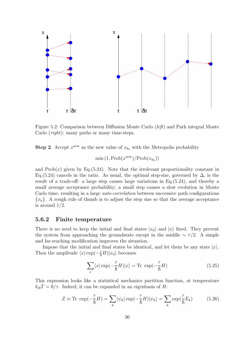
To go from Diffusion Monte Carlo to Path integral Monte Carlo, all that is necessary isa simple change of viewpoint, associated in practice with a different usage of computermemory, as illustrated Fig. 5.2.• Diffusion Monte Carlo considers many walkers {xj} at one imaginary time τ = kδτ .• Path integral Monte Carlo considers one walker at many times, i.e. one path x(τ).
One practical advantage is that the weights of the walkers, with their undesirablefluctuations, can now be eliminated. Importance sampling can be implemented exactly,using e.g. the Metropolis algorithm. To see this, rewrite the transition amplitudeEq.(5.14) in imaginary time τ = it:
〈x| exp(−τ~H)|x0〉 =
∫
dx1dx2..dxN−1
N∏
k=1
〈xk| exp(−δτ~H)|xk−1〉
≈ CN
∫
dx1dx2..dxN−1
N∏
k=1
exp
[
−δτ~
(
+1
2m(
xk − xk−1
δτ)2 +
V (xk) + V (xk−1)
2
)]
= CN
∫
dx1dx2..dxN−1〈x| exp
[
−δτ~
(
+1
2m∑
k
(xk − xk−1
δτ)2 +
∑
k
V (xk) + V (xk−1)
2
)]
|x0〉
(5.23)
This represents the desired stationary distribution of the Markov chain correspondingto our Monte Carlo process. To converge to this distribution, starting from an arbitraryconfiguration (e.g. xk = 0 ∀k), perform many sweeps, where one sweep consists of up-dating once each xk0 , keeping all xk, k 6= k0 fixed. The induced probability distributionfor xk0 is, up to an irrelevant proportionality constant:
Prob(xk0) ∝ exp
[
−δτ~
(
+1
2m
(
(
xk0+1 − xk0δτ
)2
+
(
xk0 − xk0−1
δτ
)2)
+ V (xk0)
)]
(5.24)Therefore, a Metropolis update of xk0 is implemented as:Step 1. Propose a candidate xnew = xk0 + δx, where δx is drawn from an even distri-bution (e.g. uniform in [−∆,+∆]).
35
x
τ + δττ
x
τ + δττ
Figure 5.2: Comparison between Diffusion Monte Carlo (left) and Path integral MonteCarlo (right): many paths or many time-steps.
Step 2. Accept xnew as the new value of xk0 with the Metropolis probability
min (1,Prob(xnew)/Prob(xk0))
and Prob(x) given by Eq.(5.24). Note that the irrelevant proportionality constant inEq.(5.24) cancels in the ratio. As usual, the optimal step-size, governed by ∆, is theresult of a trade-off: a large step causes large variations in Eq.(5.24), and thereby asmall average acceptance probability; a small step causes a slow evolution in MonteCarlo time, resulting in a large auto-correlation between successive path configurations{xk}. A rough rule of thumb is to adjust the step size so that the average acceptanceis around 1/2.
5.6.2 Finite temperature
There is no need to keep the initial and final states |x0〉 and |x〉 fixed. They preventthe system from approaching the groundstate except in the middle ∼ τ/2. A simpleand far-reaching modification improves the situation.
Impose that the initial and final states be identical, and let them be any state |x〉.Then the amplitude 〈x| exp(− τ
~H)|x0〉 becomes
∑
x
〈x| exp(−τ~H)|x〉 = Tr exp(−τ
~H) (5.25)
This expression looks like a statistical mechanics partition function, at temperaturekBT = ~/τ . Indeed, it can be expanded in an eigenbasis of H :
Z ≡ Tr exp(−τ~H) =
∑
k
〈ψk| exp(−τ~H)|ψk〉 =
∑
k
exp(τ
~Ek) (5.26)
36
x
τ
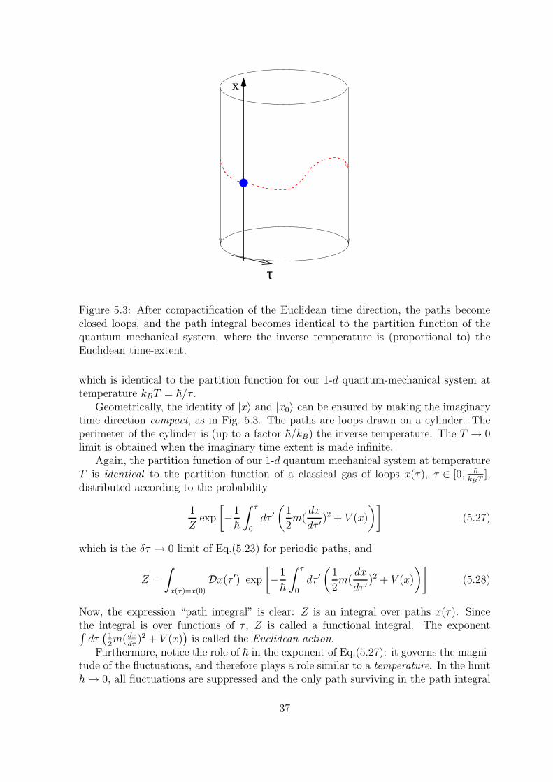
Figure 5.3: After compactification of the Euclidean time direction, the paths becomeclosed loops, and the path integral becomes identical to the partition function of thequantum mechanical system, where the inverse temperature is (proportional to) theEuclidean time-extent.
which is identical to the partition function for our 1-d quantum-mechanical system attemperature kBT = ~/τ .
Geometrically, the identity of |x〉 and |x0〉 can be ensured by making the imaginarytime direction compact, as in Fig. 5.3. The paths are loops drawn on a cylinder. Theperimeter of the cylinder is (up to a factor ~/kB) the inverse temperature. The T → 0limit is obtained when the imaginary time extent is made infinite.
Again, the partition function of our 1-d quantum mechanical system at temperatureT is identical to the partition function of a classical gas of loops x(τ), τ ∈ [0, ~
kBT],
distributed according to the probability
1
Zexp
[
−1
~
∫ τ
0
dτ ′(
1
2m(
dx
dτ ′)2 + V (x)
)]
(5.27)
which is the δτ → 0 limit of Eq.(5.23) for periodic paths, and
Z =
∫
x(τ)=x(0)
Dx(τ ′) exp
[
−1
~
∫ τ
0
dτ ′(
1
2m(
dx
dτ ′)2 + V (x)
)]
(5.28)
Now, the expression “path integral” is clear: Z is an integral over paths x(τ). Sincethe integral is over functions of τ , Z is called a functional integral. The exponent∫
dτ(
12m(dx
dτ)2 + V (x)
)
is called the Euclidean action.Furthermore, notice the role of ~ in the exponent of Eq.(5.27): it governs the magni-
tude of the fluctuations, and therefore plays a role similar to a temperature. In the limit~→ 0, all fluctuations are suppressed and the only path surviving in the path integral
37
is that which minimizes the exponent: this is the classical limit, where the path from(x0, 0) to (x, τ) is deterministic, and we recover the minimal action principle. When~ 6= 0, fluctuations are allowed around this special path: these fluctuations are quantumfluctuations.
We will consider the path integral more formally again when discussing field theoriesin Chapter 8.
5.6.3 Observables
Since one can identify the Euclidean time-extent τ of the system and its inverse tem-perature, let us use the standard notation β = 1/(kBT ) = τ/~. The expectation valueof an observable W is given by
〈W 〉 =1
ZTr (W exp(−βH)) (5.29)
which gives, when expanded in an eigenbasis of H
〈W 〉 =
∑
k〈ψk|W |ψk〉 exp(−βEk)∑
k〈ψk|ψk〉 exp(−βEk)(5.30)
=β→∞
〈ψ0|W |ψ0〉〈ψ0|ψ0〉
(5.31)
so that groundstate properties can be obtained for large Euclidean time extent.A simple example is the position projector W = |x0〉〈x0| = δ(x0). Substituting
above gives〈δ(x0)〉 =
β→∞|〈ψ0|x0〉|2 = |ψ0(x0)|2 (5.32)
so that the number of paths going through x0 (at any Euclidean time) is proportionalto the square of the wave-function.
Let us compare with Diffusion Monte Carlo: there, one had 〈δ(x0)〉 ∝ ψ0(x0), or∝ ψT (x0)ψ0(x0) when using a guiding wave-function ψT . For the optimal choice ψT = ψ0
where all walkers have weight 1, one recovers the Path integral result.One can also measure unequal-time correlations, like the two-point correlator
δ(x,∆β)δ(x, 0):
〈δ(x,∆β)δ(x, 0)〉 =
∑
k〈ψk| exp(−(β −∆β)H) δ(x) exp(−∆βH) δ(x)|ψk〉∑
k〈ψk| exp(−βH)|ψk〉
=
∑
k,l |〈ψk|δ(x)|ψl〉|2 exp(−(β −∆β)Ek) exp(−∆βEl)∑
k exp(−βEk)≈
β,∆β→∞|〈ψ0|δ(x)|ψ0〉|2 + |〈ψ1|δ(x)|ψ0〉|2 exp(−∆β(E1 − E0)) + · · ·
(5.33)
where a complete set of states∑
l |ψl〉〈ψl| was inserted to go from the first to the secondline. The final expression shows that the connected correlator 〈δ(x,∆β)δ(x, 0)〉−〈δ(x)〉2approaches 0 exponentially fast, and that the rate of decay (in Euclidean time ∆β) givesthe energy gap (E1 −E0) between the groundstate and the first excited state.
38
The groundstate energy itself is more delicate to obtain, for the following reason.Consider the kinetic energy part of Eq.(5.23). It defines a Gaussian distribution for(xk−xk−1), with variance 〈(xk−xk−1)
2〉 ∼ O(δτ), as appropriate for Brownian motion:the mean-square distance grows linearly with time. However, this implies that themean-sqare velocity 〈(xk−xk−1
δτ)2〉, i.e. the kinetic energy, grows as 1/δτ . This is, again,
expected from Brownian motion: a Brownian path is continuous, but not differentiable(it is full of kinks). As a result, the reference groundstate energy is infinite when δτ → 0.
A way around this problem is to adopt a different definition of the kinetic energy,replacing (xk−xk−1)
2 by a “split-point” alternative (xk+1−xk)(xk−xk−1). Alternatively,
one can make use of the virial theorem which gives for the kinetic energy 〈 p22m〉 = 1
2〈xdV
dx〉.
See exercises.
5.6.4 Monte Carlo simulation
The Monte Carlo simulation samples paths x(τ), discretized at N points. Thus, theconfiguration of the system at any step of the Markov chain is defined by the positions{xk, k = 1, .., N}. To manipulate dimensionless numbers, set ~ = 1 and use the con-ventional notation a ≡ δτ . a, which is called the lattice spacing has the dimension oftime (equivalently, of length). Dimensionless variables are
m = am
x = x/a
V (x) = aV (x)
T = aT = 1/N
The probability of a path {xk, k = 1, .., N} is given by Eq.(5.23):
1
Zexp
[
−(
1
2m∑
k
(xk − xk−1)2 +
∑
k
V (xk)
)]
(5.34)
and can be sampled with the Metropolis algorithm, as already outlined. Two require-ments must be kept in mind:• For the groundstate to dominate the partition function, the temperature must besmall enough that the excited states have decayed away, namely β(E1 − E0) ≫ 1. Indimensionless units, this translates into
N ≫ (E1 − E0)−1 (5.35)
In other words, a clear exponential decay of the connected correlation Eq.(5.33) mustbe observed. Violation of this requirement can be interpreted as a finite-size effect.• For discretization errors O(a2) to be small, all correlation lengths must be largecompared to a. This translates into
(E1 − E0)−1 ≫ 1 (5.36)
For the harmonic oscillator V (x) = 12ω2x2, these two requirements become 1≪ ω−1 ≪
N . The idea is to reduce ω, so that a continuum extrapolation a→ 0 can be performed,
39
while keeping the temperature low enough. While doing so, the computer requirementsincrease for two reasons: N increases, and the number of Monte Carlo sweeps requiredto obtain a statistically uncorrelated path increases too. The latter phenomenon iscalled critical slowing down. It can be largely alleviated, in the quantum-mechanicalcase, by cluster or loop algorithms.
5.6.5 Useful references
• A statistical approach to Quantum Mechanics, by M. Creutz and B. Freedman,Annals of Physics 132 (1981) 427.
• A Java demonstration of Path integral Monte Carlo by A. Santamaria can befound at http://fisteo12.ific.uv.es/∼santamar/qapplet/metro.html. Note that theparameters of the quartic potential can be adjusted interactively.
40
Chapter 6
Electronic structure of moleculesand atoms
6.1 Introduction
In this chapter we will discuss the arguably most important quantum many body prob-lem – the electronic structure problem – relevant for almost all properties of matterrelevant in our daily life. With O(1023) atoms in a typical piece of matter, the exponen-tial scaling of the Hilbert space dimension with the number of particles is a nightmare.In this chapter we will discuss approximations used in quantum chemistry that reducethe problem to a polynomial one, typically scaling like O(N4). These methods mapthe problem to a single-particle problem and work only as long as correlations betweenelectrons are weak. In the following we will discuss exact methods - without any ap-proximation - which are needed for the simulation of strongly correlated systems, suchas high temperature superconductors, heavy electron materials and quantum magnets.
6.2 The electronic structure problem
For many atoms (with the notable exception of Hydrogen and Helium which are so lightthat quantum effects are importanr in daily life), the nuclei of atoms are so much heavierthan the electrons that we can view them as classical particles and can consider themas stationary for the purpose of calculating the properties of the electrons. Using thisBorn-Oppenheimer approximation the Hamiltonian operator for the electrons becomes
H =
N∑
i=1
(
− ~2
2m∇2 + V (~ri)
)
+ e2∑
i<j
e2
|~ri − ~rj|(6.1)
where the potential of the M atomic nuclei with charges Zi at the locations ~Ri is givenby
V (~r) = −e2M∑
i=1
Zi
|~Ri − ~r|. (6.2)
41
The Car-Parinello method for molecular dynamics, which we will discuss later, movesthe nuclei classically according to electronic forces that are calculated quantum mechan-ically.
Using a basis set of L orbital wave functions {fi}, the matrix elements of the Hamil-ton operator (6.1) are
tij =
∫
d3~rf ∗i (~r)
(
~2
2m∇2 + V (~r)
)
fj(~r) (6.3)
Vijkl = e2∫
d3~r
∫
d3~r′f ∗i (~r)fj(~r)1
|~r − ~r′|f∗k (~r′)fl(~r
′) (6.4)
and the Hamilton operator can be written in second quantized notation as
H =∑
ijσ
tija†iσajσ +
1
2
∑
ijklσσ′
Vijkla†iσa†kσ′alσ′ajσ. (6.5)
6.3 Basis functions
Before attempting to solve the many body problem we will discuss basis sets for singleparticle wave functions.
6.3.1 The electron gas
For the free electron gas with Hamilton operator
H = −N∑
i=1
~2
2m∇2 + e2
∑
i<j
vee(~ri, ~rj) (6.6)
vee(~r, ~r′) =
1
|~r − ~r′| (6.7)
the ideal choice for basis functions are plane waves
ψ~k(~r) = exp(−i~k~r). (6.8)
Such plane wave basis functions are also commonly used for band structure calculationsof periodic crystals.
At low temperatures the electron gas forms a Wigner crystal. Then a better choice ofbasis functions are eigenfunctions of harmonic oscillators centered around the classicalequilibrium positions.
6.3.2 Atoms and molecules
Which functions should be used as basis functions for atoms and molecules? We can letourselves be guided by the exact solution of the Hydrogen atom and use the so-calledSlater-Type-Orbitals (STO):
finlm(r, θ, φ) ∝ rn−1e−ζirYlm(θ, φ). (6.9)
42
These wave functions have the correct asymptotic radial dependence and the correctangular dependence. The values ζi are optimized so that the eigenstates of isolatedatoms are reproduced as accurately as possible.
The main disadvantage of the STOs becomes apparent when trying to evaluatethe matrix elements in equation (6.4) for basis functions centered around two different
nuclei at position ~RA and ~RB. There we have to evaluate integrals containing termslike
1
~r − ~r′e−ζi|~r−
~RA|e−ζj |~r−~RB | (6.10)
which cannot be solved in any closed form.The Gauss-Type-Orbitals (GTO)
filmn(~r) ∝ xlymzne−ζir2
(6.11)
simplify the evaluation of matrix elements, as Gaussian functions can be integratedeasily and the product of Gaussian functions centered at two different nuclei is again asingle Gaussian function:
e−ζi|~r−~RA|2e−ζj |~r−
~RB |2 = Ke−ζ|~r−~R|2 (6.12)
with
K = e− ζiζj
ζi+ζj|~RA− ~RB |2
(6.13)
ζ = ζi + ζj (6.14)
~R =ζi ~RA + ζj ~RB
ζi + ζj(6.15)
Also the term 1|~r−~r′| can be rewritten as an integral over a Gaussian function
1
|~r − ~r′| =2√π
∫ ∞
0
dte−t2(~r−~r′)2 . (6.16)
and thus all the integrals (6.4) reduce to purely Gaussian integrals which can be per-formed analytically.
As there are O(L4) integrals of the type (6.4), quantum chemistry calculations typ-ically scale as O(N4). Modern methods can be used to reduce the effort to an approx-imately O(N) method, since the overlap of basis functions at large distances becomesnegligibly small.
Independent of whether one chooses STOs or GTOs, extra care must be taken toaccount for the non-orthogonality of these basis functions.
6.4 Pseudo-potentials
The electrons in inner, fully occupied shells do not contribute in the chemical bindings.To simplify the calculations they can be replaced by pseudo-potentials, modeling theinner shells. Only the outer shells (including the valence shells) are then modeled usingbasis functions. The pseudo-potentials are chosen such that calculations for isolatedatoms are as accurate as possible.
43
6.5 The Hartree Fock method
6.5.1 The Hartree-Fock approximation
The Hartree-Fock approximation is based on the assumption of independent electrons.It starts from an ansatz for the N -particle wave function as a Slater determinant of Nsingle-particle wave functions:
Φ(~r1, σ1; . . . ;~rN , σN) =1√N
∣
∣
∣
∣
∣
∣
∣
φ1(~r1, σ1) · · · φN(~r1, σ1)...
...φ1(~rN , σN) · · · φN(~rN , σN)
∣
∣
∣
∣
∣
∣
∣
. (6.17)
The orthogonal single particle wave functions φµ are chosen so that the energy isminimized.
For numerical calculations a finite basis has to be introduced, as discussed in theprevious section. Quantum chemists distinguish between the self-consistent-field (SCF)approximation in a finite basis set and the Hartree-Fock (HF) limit, working in a com-plete basis. In physics both are known as Hartree-Fock approximation.
6.5.2 The Hartree-Fock equations in nonorthogonal basis sets
It will be easiest to perform the derivation of the Hartree-Fock equations in a secondquantized notation. To simplify the discussion we assume closed-shell conditions, whereeach orbital is occupied by both an electron with spin ↑ and one with spin ↓. We startby writing the Hartree Fock wave function (6.17) in second quantized form:
|Φ〉 =∏
µ,σ
c†µσ|0〉, (6.18)
where c†µσ creates an electron in the orbital φµ(r, σ). As these wave functions are or-thogonal the c†µσ satsify the usual fermion anticommutation relations. Greek subscriptsrefer to the Hartree-Fock single particle orbitals and roman subscripts to the singleparticle basis functions. Next we expand the c†µσ in terms of the creation operators a†nσof our finite basis set:
c†µσ =
L∑
n=1
dµna†nσ (6.19)
and find thatajσ|Φ〉 = ajσ
∏
µ,σ′
c†µσ′ |0〉 =∑
ν
dνj∏
µσ′ 6=νσc†µσ′ |0〉. (6.20)
In order to evaluate the matrix elements 〈Φ|H|Φ〉 of the Hamiltonian (6.5) we introducethe bond-order matrix
Pij =∑
σ
〈Φ|a†iσajσ|Φ〉 = 2∑
ν
d∗νidνj, (6.21)
where we have made use of the closed-shell conditions to sum over the spin degreesof freedom. The kinetic term of H is now simply
∑
ij Pijtij . Next we rewrite the
44
interaction part 〈Φ|a†iσa†kσ′alσ′ajσ|Φ〉 in terms of the Pij. We find that if σ = σ′
〈Φ|a†iσa†kσalσajσ|Φ〉 = 〈Φ|a†iσajσ|Φ〉〈Φ|a†kσalσ|Φ〉 − 〈Φ|a†iσalσ|Φ〉〈Φ|a†kσajσ|Φ〉 (6.22)
and if σ 6= σ′:〈Φ|a†iσa†kσ′alσ′ajσ|Φ〉 = 〈Φ|a†iσajσ|Φ〉〈Φ|a†kσ′alσ′ |Φ〉 (6.23)
Then the energy is (again summing over the spin degrees of freedom):
E0 =∑
ij
tijPij +1
2
∑
ijkl
(
Vijkl −1
2Vilkj
)
PijPkl. (6.24)
We now need to minimize the energy E0 under the condition that the |φµ〉 arenormalized:
1 = 〈φµ|φµ〉 =∑
i,j
d∗µidµjSij. (6.25)
Using Lagrange multipliers to enforce this constraint we have to minimize
∑
ij
tijPij +1
2
∑
ijkl
(
Vijkl −1
2Vilkj
)
PijPkl −∑
µ
ǫµ∑
i,j
d∗µidµjSij (6.26)
Setting the derivative with respect to dµi to zero we end up with the Hartree-Fockequations for a finite basis set:
L∑
j=1
(fij − ǫµSij)dµj = 0, (6.27)
where
fij = tij +∑
kl
(
Vijkl −1
2Vilkj
)
Pkl. (6.28)
This is again a generalized eigenvalue problem of the form Ax = λBx and looks like aone-particle Schrodinger equation. However, since the potential depends on the solutionit is a nonlinear and not a linear eigenvalue problem. The equation is solved iteratively,always using the new solution for the potential, until convergence to a fixed point isachieved.
The eigenvalues ǫµ of f do not directly correspond to energies of the orbitals, as theFock operator counts the V -terms twice. Thus we obtain the total ground state energyfrom the Fock operator eigenvalues by subtracting the double counted part:
E0 =
N∑
µ=1
ǫµ −1
2
∑
ijkl
(
Vijkl −1
2Vilkj
)
PijPkl (6.29)
45
6.5.3 Configuration-Interaction
The approximations used in Hartree-Fock and density functional methods are basedon non-interacting electron pictures. They do not treat correlations and interactionsbetween electrons correctly. To improve these methods, and to allow the calculation ofexcited states, often the “configuration-interaction” (CI) method is used.
Starting from the Hartree-Fock ground state
|ψHF 〉 =N∏
µ=1
c†µ|0〉 (6.30)
one or two of the c†µ are replaced by other orbitals c†i :
|ψ0〉 =
(
1 +∑
i,µ
αiµci†cµ +∑
i<j,µ<ν
αijµνci†cj†cµcν)
|ψHF 〉. (6.31)
The energies are then minimized using this variational ansatz. In a problem withN occupied and M empty orbitals this leads to a matrix eigenvalue problem withdimension 1+NM+N2M2. Using the Lanczos algorithm the low lying eigenstates canthen be calculated in O((N +M)2) steps.
Further improvements are possible by allowing more than only double-substitutions.The optimal method treats the full quantum problem of dimension (N + M)!/N !M !.Quantum chemists call this method “full-CI”. Physicists simplify the Hamilton operatorslightly to obtain simpler models with fewer matrix elements, and call that method“exact diagonalization”. This method will be discussed later in the course.
6.6 Density functional theory
Another commonly used method, for which the Nobel prize in chemistry was awardedto Walter Kohn, is the density functional theory. In density functional theory themany-body wave function living in R3N is replaced by the electron density, which livesjust in R3. Density functional theory again reduces the many body problem to a one-dimensional problem. In contrast to Hartree-Fock theory it has the advantage that itcould – in principle – be exact if there were not the small problem of the unknownexchange-correlation functional.
It is based on two fundamental theorems by Hohenberg and Kohn. The first theoremstates that the ground state energy E0 of an electronic system in an external potentialV is a functional of the electron density ρ(~r) :
E0 = E[ρ] =
∫
d3~rV (~r)ρ(~r) + F [ρ], (6.32)
with a universal functional F . The second theorem states that the density of the groundstate wave function minimizes this functional. The proof of both theorems will be shownin the lecture.
46
These theorems make our life very easy: we only have to minimize the energyfunctional and we obtain both the ground state energy and the electron density in theground state – and everything is exact!
The problem is that, while the functional F is universal, it is also unknown! Thuswe need to find good approximations for the functional. One usually starts from theansatz:
F [ρ] = Eh[ρ] + Ek[ρ] + Exc[ρ]. (6.33)
The Hartree-term Eh given by the Coulomb repulsion between two electrons:
Eh[ρ] =e2
2
∫
d3~rd3~r′ρ(~r)ρ(~r′)
|~r − ~r′| . (6.34)
The kinetic energy Ek[ρ] is that of a non-interacting electron gas with the same density.The exchange- and correlation term Exc[ρ] contains the remaining unknown contribu-tion, which we will discuss a bit later.
To calculate the ground state density we have to minimize this energy, solving thevariational problem
0 = δE[ρ] =
∫
d3~rδρ(~r)
(
V (~r) + e2∫
d3~r′ρ(~r′)
|~r − ~r′| +δEk[ρ]
δρ(~r)+δExc[ρ]
δρ(~r)
)
(6.35)
0 subject to the constraint that the total electron number to be conserved∫
d3~rδρ(~r) = 0. (6.36)
Comparing this variational equation to the one for noninteracting system(
− 1
2m∇2 + Veff(~r)
)
φµ(~r) = ǫµφµ(~r), (6.37)
we realize that they are the same if we define the potential of the non-interacting systemas
Veff (~r) = V (~r) + e2∫
d3~r′ρ(~r′)
|~r − ~r′| + vxc(~r), (6.38)
where the exchange-correlation potential is defined by
vxc(~r) =δExc[ρ]
δρ(~r). (6.39)
The form (6.37) arises because we have separated the kinetic energy of the non-interactingelectron system from the functional. The variation of this kinetic energy just gives thekinetic term of this Schrodinger-like equation.
The non-linear equation is again solved iteratively, making an ansatz using N/2normalized single-electron wave functions, which we occupy with spin ↑ and spin ↓electrons to get the electron density.
ρ(~r) = 2
N/2∑
µ=1
|φµ(~r)|2, (6.40)
47
6.6.1 Local Density Approximation
Apart from the restricted basis set everything was exact up to this point. As thefunctional Exc[ρ] and thus the potential vxc(~r) is not known, we need to introduceapproximations.
The simplest approximation is the “local density approximation” (LDA), whichreplaces vxc by that of a uniform electron gas with the same density. Instead of takinga functional E[ρ](~r) which could be a function of ρ(~r),∇ρ(~r),∇∇ρ(~r), . . . we ignore allthe gradients and just take the local density
Exc[ρ](r) = ELDA(ρ(r)); (6.41)
Defining
r−1s = aB
(
4π
3ρ
)1/3
(6.42)
the exchange correlation potential is
vxc = − e2
aB
(
3
2π
)2/31
rs[1 + 0.0545rs ln(1 + 11.4/rs)] (6.43)
where the first part corresponds to uncorrelated electrons and the last factor is a cor-relation correction determined by fitting to quantum Monte Carlo (QMC) simulationsof an electron gas.
6.6.2 Improved approximations
Improvements over the LDA have been an intense field of research in quantum chemistry.I will just mention two improvements. The “local spin density approximation” (LSDA)uses separate densities for electrons with spin ↑ and ↓. The “generalized gradientapproximation” (GGA) and its variants use functionals depending not only on thedensity, but also on its derivatives.
6.7 Car-Parinello molecular dynamics
In the lecture on “Computational Statistical Physics” you have learned about the molec-ular dynamics method, in which atoms move on classical trajectories under forces, suchas those from the Lennard-Jones potential, which have been previously calculated inquantum mechanical simulations. It would be nicer, and more accurate, to use a fullquantum mechanical force calculation at every time step instead of using such staticforces that have been extracted from previous simulations.
Roberto Car (currently in Princeton) and Michele Parinello (currently at ETH) havecombined density functional theory with molecular dynamics to do just that. Theirmethod, Car-Parinello molecular dynamics (CPMD) allows much better simulations ofmolecular vibration spectra and of chemical reactions.
48
The atomic nuclei are propagated using classical molecular dynamics, but the elec-tronic forces which move them are estimated using density functional theory:
Mnd2 ~Rn
dt2= −∂E[ρ(~r, t), ~Rn]
∂ ~Rn
. (6.44)
Here Mn and ~Rn are the masses and locations of the atomic nuclei.As the solution of the full electronic problem at every time step is a very time
consuming task we do not want to perform it all the time from scratch. Instead CPMDuses the previous values of the noninteracting electron wave functions {φµ} of the DFTcalculation (6.37) [don’t confuse it with the Hartee-Fock orbitals!] and evolves themto the ground state for the current positions of the nuclei by an artificial moleculardynamics evolution. Hence both the nuclei {~Rn} and the wave functions {φµ} evolve inthe same molecular dynamics scheme. The electronic degrees of freedoms are updatedusing an artificial dynamics:
md2φµ(~r, t)
dt2= −1
2
δE[ρ(~r, t), ~Rn]
δφ†µ(~r, t)+∑
ν
Λµνφν(~r, t), (6.45)
where m is an artificial mass that needs to be chosen much lighter than the nuclearmasses so that the electronic structure adapts quickly to the move of the nuclei. TheLagrange multipliers Λµν need to be chose to ensure proper orthonormalization of thewave functions.
Since the exact form of the artifical dynamics of the electronic structure does notmatter, we can evolve the expansion coefficients dµn of an expansion in terms of thebasis functions as in equation (6.19) instead of evolving the wave functions. This givesthe equations of motion
md2dµndt2
= − ∂E
∂dµn+∑
ν
Λµν
∑
l
Snldνl (6.46)
There are various algorithms to determine the Λµν so that the wave functions stayorthonormal. We refer to text books and special lectures on CPMD for details.
6.8 Program packages
As the model Hamiltonian and the types of basis sets are essentially the same for allquantum chemistry applications flexible program packages have been written. Thereis thus usually no need to write your own programs – unless you want to implement anew algorithm.
49
Chapter 7
Exact diagonalization of thequantum many body problem
The quantum chemical approaches discussed in the previous chapter simplify the prob-lem of solving a quantum many body problem. The complexity of a problem withN particles in M = O(N) orbitals is then only O(N4) or often better, instead ofO(exp(N)).
This enormous reduction in complexity is however paid for by a crude approximationof electron correlation effects. This is acceptable for normal metals, band insulators andsemi-conductors but fails in materials with strong electron correlations, such as almostall transition metal ceramics.
In the last category many new materials have been synthesized over the past twentyyears, including the famous high temperature superconductors. In these materials theelectron correlations play an essential role and lead to interesting new properties that arenot completely understood yet. Here we leave quantum chemistry and enter quantumphysics again.
7.1 Models
To understand the properties of these materials the Hamilton operator of the full quan-tum chemical problem (6.1) is usually simplified to generic models, which still containthe same important features, but which are easier to investigate. They can be used tounderstand the physics of these materials, but not directly to quantitatively fit experi-ments.
7.1.1 The tight-binding model
The simplest model is the tight-binding model, which concentrates on the valence bands.All matrix elements tij in equation (6.3), apart from the ones between nearest neighboratoms are set to zero. The others are simplified, as in:
H =∑
〈i,j〉,σ(tijc
†i,σcj,σ + H.c.). (7.1)
This model is easily solvable by Fourier transforming it, as there are no interactions.
50
7.1.2 The Hubbard model
To include effects of electron correlations, the Hubbard model includes only the oftendominant intra-orbital repulsion Viiii of the Vijkl in equation (6.4):
H =∑
〈i,j〉,σ(tijc
†i,σcj,σ + H.c.) +
∑
i
Uini,↑ni,↓. (7.2)
The Hubbard model is a long-studied, but except for the 1D case still not completelyunderstood model for correlated electron systems.
In contrast to band insulators, which are insulators because all bands are eithercompletely filled or empty, the Hubbard model at large U is insulating at half filling,when there is one electron per orbital. The reason is the strong Coulomb repulsion Ubetween the electrons, which prohibit any electron movement in the half filled case atlow temperatures.
7.1.3 The Heisenberg model
In this insulating state the Hubbard model can be simplified to a quantum Heisenbergmodel, containing exactly one spin per site.
H =∑
〈i,j〉Jij ~Si~Sj (7.3)
For large U/t the perturbation expansion gives Jij = 2t2ij(1/Ui+1/Uj). The Heisenbergmodel is the relevant effective models at temperatures T ≪ tij , U ( 104 K in copperoxides). The derivation will be shown in the lecture.
7.1.4 The t-J model
The t-J model is the effective model for large U at low temperatures away from half-filling. Its Hamiltonian is
H =∑
〈i,j〉,σ
[
(1− ni,−σ)tijc†i,σcj,σ(1− nj,−σ) + H.c.]
+∑
〈i,j〉Jij(~Si~Sj − ninj/4). (7.4)
As double-occupancy is prohibited in the t-J model there are only three instead of fourstates per orbital, greatly reducing the Hilbert space size.
7.2 Exact diagonalization
The most accurate method is exact diagonalization of the Hamiltonian matrix usingthe Lanczos algorithm, discussed in appendix A.2. The size of the Hilbert space of anN -site system [4N for a Hubbard model , 3N for a t-J model and (2S+1)N for a spin-Smodel] can be reduced by making use of symmetries. Translational symmetries can beemployed by using Bloch waves with fixed momentum as basis states. Conservation of
51
particle number and spin allows to restrict a calculation to subspaces of fixed particlenumber and magnetization.
As an example we will sketch how to implement exact diagonalization for a simpleone-dimensional spinless fermion model with nearest neighbor hopping t and nearestneighbor repulsion V :
H = −tL−1∑
i=1
(c†ici+1 + H.c.) + V
L−1∑
i=1
nini+1. (7.5)
The first step is to construct a basis set. We describe a basis state using “multi-bitcoding”. A many-body state of fermions on up to 32 sites is represented as an unsignedinteger where bit i set to one corresponds to an occupied site i. For spinful fermions wetake either two integers, one for the up and one for the down spins, or two bits per site.
As the Hamiltonian conserves the total particle number we thus want to constructa basis of all states with N particles on L sites (or N bits set to one in L bits). In thefollowing code fragment we use the following variables:
• states is a vector storing the integers whose bit patterns correspond to the basisstates. It can be accessed using the following functions:
– dimension() returns the number of basis states.
– state(i) returns the i-th basis state, where i runs from 0 to dimension()−1.
• index is a much larger vector of size 2L. It is used to obtain the number of astate in the basis, given the integer representation of the state. It can be accessedusing the function
– index(s) which returns the index i of the state in the basis, or the largestinteger to denote an invalid state, if the bit pattern of the integer does notcorrespond to a basis state.
Since this vector is very large, it will limit the size of system that can be studied.To save space, the index array could be omitted and the index(s) functionimplemented by a binary search on the states array.
Here is the C++ code for this class:
#include <vector>
#include <alps/bitops.h>
#include <limits>
#include <valarray>
#include <cassert>
class FermionBasis {
public:
typedef unsigned int state_type;
typedef unsigned int index_type;
52
FermionBasis (int L, int N);
state_type state(index_type i) const {return states_[i];}
index_type index(state_type s) const {return index_[s];}
unsigned int dimension() const { return states_.size();}
private:
std::vector<state_type> states_;
std::vector<index_type> index_;
};
In the constructor we build the basis states. For N spinless fermions on L sites thevalid basis states are all the ways to place N particles on L sites, which is equivalentto all integers between 0 and 2L − 1 that have N bits set. The constructor uses thealps::popcnt function of the ALPS library.
FermionBasis::FermionBasis(int L, int N)
{
index_.resize(1<<L); // 2^L entries
for (state_type s=0;s<index_.size();++s)
if(alps::popcnt(s)==N) {
// correct number of particles
states_.push_back(s);
index_[s]=states_.size()-1;
}
else
// invalid state
index_[s]=std::numeric_limits<index_type>::max();
}
Finally we want to implement a matrix-vector multiplication v = Hw for our Hamil-tonian and derive a Hamiltonian class. We do not want to store the matrix at all,neither in dense nor in sparse form but instead implement a fast function to performthe matrix-vector multiplication on-the-fly.
class HamiltonianMatrix : public FermionBasis {
public:
HamiltonianMatrix(int L, int N, double t, double V)
: FermionBasis(L,N), t_(t), V_(V), L_(L) {}
void multiply(std::valarray<double>& v, const std::valarray<double>& w);
private:
double t_, V_;
int L_;
};
53
Finally we show the implementation of the matrix-vector multiplication. It might looklike magic but we will explain it all in detail during the lecture.
void HamiltonianMatrix::multiply(std::valarray<double>& v,
const std::valarray<double>& w)
{
// check dimensions
assert(v.size()==dimension());
assert(w.size()==dimension());
// do the V-term
for (int i=0;i<dimension();++i) {
state_type s = state(i);
// count number of neighboring fermion pairs
v[i]=w[i]*V_*alps::popcnt(s&(s>>1));
}
// do the t-term
for (int i=0;i<dimension();++i) {
state_type s = state(i);
// inside the chain
for (int r=0;r<L_-1;++r) {
state_type shop = s^(3<<r); // exchange two neighbors
index_type idx = index(shop); // get the index
if(idx!=std::numeric_limits<index_type>::max())
v[idx]+=-t_*w[i];
}
// across the boundary
state_type shop = s^(1|(1<<(L-1))); // exchange the first and last
index_type idx = index(shop); // get the index
if(idx!=std::numeric_limits<index_type>::max())
// watch out for Fermi sign since we hop over some particles
v[idx]+=-t*(alps::popcnt(s&((1<<(L-1))-1))%2==0 ? 1 : -1)*w[i];
}
}
This class can now be used together with the Lanczos algorithm to calculate theenergies and wave functions of the low lying states of the Hamiltonian.
In production codes one uses all symmetries to reduce the dimension of the Hilbertspace as much as possible. In this example translational symmetry can be used ifperiodic boundary conditions are applied. The implementation gets much harder then.
In order to make the implementation of exact diagonalization much easier we havegeneralized the expression templates technique developed by Todd Veldhuizen for arrayexpression to expressions including quantum operators. Using this expression template
54
library we can write a multiplication
|ψ〉 = H|φ〉 = (−tL−1∑
i=1
(c†ici+1 + H.c.) + V
L−1∑
i
nini+1)|φ〉 (7.6)
simply as:
Range i(1,L-1);
psi = sum(i,(-t*(cdag(i)*c(i+1)+HermitianConjugate)+V*n(i)*n(i+1))*phi);
The advantage of the above on-the-fly calculation of the matrix in the multiplicationroutine is that the matrix need not be stored in memory, which is an advantage for thebiggest systems where just a few vectors of the Hilbert space will fit into memory.
If one is not as demanding and wants to simulate a slightly smaller system, wherethe (sparse) matrix can be stored in memory, then a less efficient but more flexiblefunction can be used to create the matrix and store it in memory. Such a programis available through the ALPS project at http://alps.comp-phys.org/. It allows toperform the above calculation just by describing the lattice and model in an XML inputfile.
55
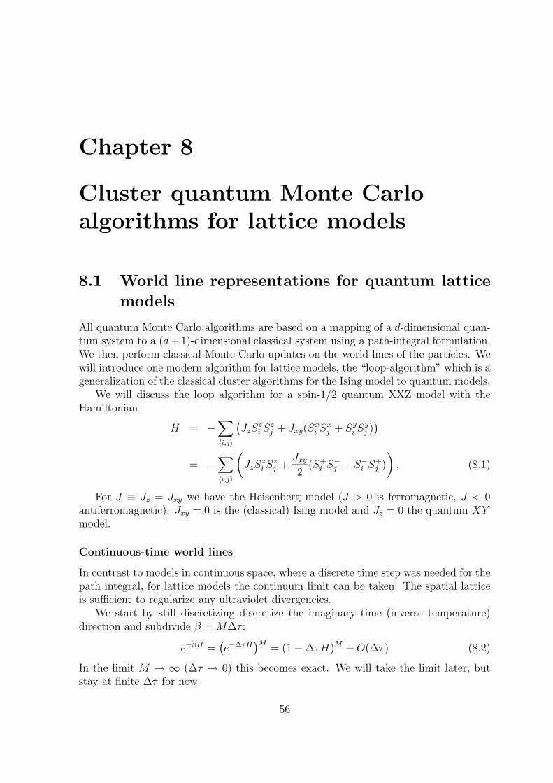
Chapter 8
Cluster quantum Monte Carloalgorithms for lattice models
8.1 World line representations for quantum lattice
models
All quantum Monte Carlo algorithms are based on a mapping of a d-dimensional quan-tum system to a (d+1)-dimensional classical system using a path-integral formulation.We then perform classical Monte Carlo updates on the world lines of the particles. Wewill introduce one modern algorithm for lattice models, the “loop-algorithm” which is ageneralization of the classical cluster algorithms for the Ising model to quantum models.
We will discuss the loop algorithm for a spin-1/2 quantum XXZ model with theHamiltonian
H = −∑
〈i,j〉
(
JzSzi S
zj + Jxy(S
xi S
xj + Syi S
yj ))
= −∑
〈i,j〉
(
JzSzi S
zj +
Jxy2
(S+i S−j + S−i S
+j )
)
. (8.1)
For J ≡ Jz = Jxy we have the Heisenberg model (J > 0 is ferromagnetic, J < 0antiferromagnetic). Jxy = 0 is the (classical) Ising model and Jz = 0 the quantum XYmodel.
Continuous-time world lines
In contrast to models in continuous space, where a discrete time step was needed for thepath integral, for lattice models the continuum limit can be taken. The spatial latticeis sufficient to regularize any ultraviolet divergencies.
We start by still discretizing discretize the imaginary time (inverse temperature)direction and subdivide β = M∆τ :
e−βH =(
e−∆τH)M
= (1−∆τH)M +O(∆τ) (8.2)
In the limit M → ∞ (∆τ → 0) this becomes exact. We will take the limit later, butstay at finite ∆τ for now.
56
space
imag
inar
y tim
e
0
β
Figure 8.1: Example of a world line configuration for a spin-1/2 quantum Heisenbergmodel. Drawn are the world lines for up-spins only. Down spin world lines occupy therest of the configuration.
The next step is to insert the identity matrix, represented by a sum over all basisstates 1 =
∑
i |i〉〈i| between all operators (1−∆τH):
Z = Tre−βH = Tr (1−∆τH)M +O(∆τ)
=∑
i1,...,iM
〈i1|1−∆τH|i2〉〈i2|1−∆τH|i3〉 · · · 〈iM |1−∆τH|i1〉+O(∆τ)
=: Pi1,...,iM (8.3)
and similarly for the measurement, obtaining
〈A〉 =∑
i1,...,iM
〈i1|A(1−∆τH)|i2〉〈i1|1−∆τH|i2〉
Pi1,...,iM +O(∆τ). (8.4)
If we choose the basis states |i〉 to be eigenstates of the local Sz operators we endup with an Ising-like spin system in one higher dimension. Each choice i1, . . . , iMcorresponds to one of the possible configurations of this classical spin system. Thetrace is mapped to periodic boundary conditions in the imaginary time direction of thisclassical spin system. The probabilities are given by matrix elements 〈in|1−∆τH|in+1〉.We can now sample this classical system using classical Monte Carlo methods.
However, most of the matrix elements 〈in|1−∆τH|in+1〉 are zero, and thus nearly allconfigurations have vanishing weight. The only non-zero configurations are those whereneighboring states |in〉 and |in+1〉 are either equal or differ by one of the off-diagonalmatrix elements in H , which are nearest neighbor exchanges by two opposite spins. Wecan thus uniquely connect spins on neighboring “time slices” and end up with worldlines of the spins, sketched in Fig. 8.1. Instead of sampling over all configurations oflocal spins we thus have to sample only over all world line configurations (the othershave vanishing weight). Our update moves are not allowed to break world lines buthave to lead to new valid world line configurations.
Finally we take the continuous time limit ∆τ → 0. Instead of storing the configura-tions at all M →∞ time steps, we will not just store the times τ where a spin flips as
57
the consequence of an off-diagonal operator acting at that time. The number of suchevents stays finite as M →∞: as can be seen from equation (8.2) the probability of Hacting at a given time is proportional to 1/M , and hence the total number of spin flipswill stay finite although M →∞
8.1.1 The stochastic series expansion (SSE)
An alternative representation, which is easier to code, is the stochastic series expansion(SSE) method, developed by Anders Sandvik.1 We start from a high temperature seriesexpansion of the partition function, which is just a Taylor series
Z = Tre−βH =
∞∑
n=0
∑
α
βn
n!〈α|(−H)n|α〉 (8.5)
where {|α〉} now denotes the basis states.2 The next step is to decompose the Hamil-tonian into a sum of bond Hamiltonians
H =M∑
b=1
Hb, (8.6)
where each term Hb is associated with one of the M bonds b of the lattice.We can assume that the Hamiltonian is a sum of bond terms without loss of gen-
erality. Any single-site terms, such as a local magnetic field −hSzi can be assigned tobond terms connected to the site.
Inserting this decomposition of the Hamiltonian and sets |α(p)〉 of basis vectors intothe partition function we obtain
Z =∞∑
n=0
∑
{Cn}
∑
α(0),...,α(n)
βn
n!
n∏
p=1
〈α(p)|(−Hbp)|α(p− 1)〉, (8.7)
where {Cn} denotes the set of all concatenations of n bond Hamiltonians Hb, each calledan operator string. Also, |α(n)〉 ≡ |α(0)〉, reflecting the periodicity in the propagationdirection given by the trace.
For a finite system and at finite temperature the relevant exponents of this powerseries are centered around
〈n〉 ∝ Nsβ, (8.8)
where Ns is the number of lattice sites. Hence we can truncate the infinite sum overn at a finite cut-off length Λ ∝ Nsβ without introducing any systematic error forpractical computations. The best value for Λ can be determined and adjusted duringthe equilibration part of the simulation, e.g. by setting Λ > (4/3)n after each updatestep.
1A.W. Sandvik and J. Kurkijarvi, Phys. Rev. B 43, 5950 (1991); A. W. Sandvik, J. Phys. A 25,3667 (1992).
2We switch notation here to stay consistent with the notation used in papers on the SSE method
58
Instead of working with a variable number of operators n, the code is simpler3 ifwe keep a fixed number of operators Λ. This can be done by inserting (Λ − n) unitoperators Id into every operator string of length n < Λ, and we define H0 = Id. Takingthe number of such possible insertions into account, we obtain
Z =Λ∑
n=0
∑
{CΛ}
∑
α(0),...,α(Λ)
βn(Λ− n)!
Λ!
Λ∏
p=1
〈α(p)| −Hbp|α(p− 1)〉, (8.9)
where n now denotes the number of non-unity operators in the operator string CΛ.Each such operator string is thus given by an index sequence CΛ = (b1, b2, ..., bΛ), whereon each propagation level p = 1, ...,Λ either bp = 0 for an unit operator, or 1 ≤ bp ≤Mfor a bond Hamiltonian.
Positivity of the weights
In order to interpret these weights as probabilities, all the matrix elements of −Hb needto be positive, and hence all matrix elements of Hb should be negative. For the diagonalpart of the Hamiltonian, one can assure this by subtracting a suitable constant C fromeach bond Hamiltonian.
For the off-diagonal part of the Hamiltonian an equally simple remedy does not exist.However, if only operator strings with an even number of negative matrix elements havea finite contribution to Eq. (8.9), the relative weights are again well suited to definea probability distribution. One can show that this is in general the case for bosonicmodels, ferromagnetic spin models, and antiferromagnetic spin models on bipartitelattices (such as the square lattice).
Representing the configuration
In order to represent the configurations |α(p)〉 we do not need to store the full configu-ration at avery step p, but is is sufficient to store:
• the initial state |α(0)〉
• and for each level p
– a flag indicating whether the operator at a level p is the identity, or a diagonalor off-diagonal operator
– bond bp at which each operator p acts
– the new state on the two sites of the bond bp. For spin-1/2 XXZ modelsthis is actually uniquely determined by whether the operator is diagonal oroff-diagonal and can be skipped.
3We actually recently found an way to write a simple code even with variable n, but that methodis not written up yet.
59
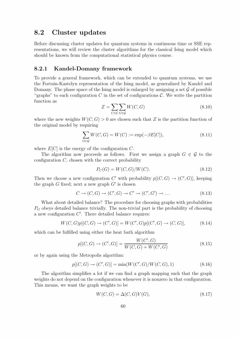
8.2 Cluster updates
Before discussing cluster updates for quantum systems in continuous time or SSE rep-resentations, we will review the cluster algorithms for the classical Ising model whichshould be known from the computational statistical physics course.
8.2.1 Kandel-Domany framework
To provide a general framework, which can be extended to quantum systems, we usethe Fortuin-Kastelyn representation of the Ising model, as generalized by Kandel andDomany. The phase space of the Ising model is enlarged by assigning a set G of possible“graphs” to each configuration C in the set of configurations C. We write the partitionfunction as
Z =∑
C∈C
∑
G∈GW (C,G) (8.10)
where the new weights W (C,G) > 0 are chosen such that Z is the partition function ofthe original model by requiring
∑
G∈GW (C,G) = W (C) := exp(−βE[C]), (8.11)
where E[C] is the energy of the configuration C.The algorithm now proceeds as follows. First we assign a graph G ∈ G to the
configuration C, chosen with the correct probability
PC(G) = W (C,G)/W (C). (8.12)
Then we choose a new configuration C ′ with probability p[(C,G) → (C ′, G)], keepingthe graph G fixed; next a new graph G′ is chosen
C → (C,G)→ (C ′, G)→ C ′ → (C ′, G′)→ . . . (8.13)
What about detailed balance? The procedure for choosing graphs with probabilitiesPG obeys detailed balance trivially. The non-trivial part is the probability of choosinga new configuration C ′. There detailed balance requires:
W (C,G)p[(C,G)→ (C ′, G)] = W (C ′, G)p[(C ′, G)→ (C,G)], (8.14)
which can be fulfilled using either the heat bath algorithm
p[(C,G)→ (C ′, G)] =W (C ′, G)
W (C,G) +W (C ′, G)(8.15)
or by again using the Metropolis algorithm:
p[(C,G)→ (C ′, G)] = min(W (C ′, G)/W (C,G), 1) (8.16)
The algorithm simplifies a lot if we can find a graph mapping such that the graphweights do not depend on the configuration whenever it is nonzero in that configuration.This means, we want the graph weights to be
W (C,G) = ∆(C,G)V (G), (8.17)
60
Table 8.1: Local bond weights for the Kandel-Domany representation of the Ising model.
c =↑↑ c =↓↑ c =↑↓ c =↓↓ V(g)∆(c, discon.) 1 1 1 1 exp(−βJ)∆(c, con.) 1 0 0 1 exp(βJ)− exp(−βJ)w(c) exp(βJ) exp(−βJ) exp(−βJ) exp(βJ)
where
∆(C,G) :=
{
1 if W (C,G) 6= 0,0 otherwise.
. (8.18)
Then equation (8.15) simply becomes p = 1/2 and equation (8.16) reduces to p = 1 forany configuration C ′ with W (C ′, G) 6= 0.
8.2.2 The cluster algorithms for the Ising model
Let us now show how this abstract and general algorithm can be applied to the Isingmodel. Our graphs will be bond-percolation graphs on the lattice. Spins pointinginto the same direction can be connected or disconnected. Spins pointing in oppositedirections will always be disconnected. In the Ising model we can write the weightsW (C) and W (C,G) as products over all bonds b:
W (C) =∏
b
w(Cb) (8.19)
W (C,G) =∏
b
w(Cb, Gb) =∏
b
∆(Cb, Gb)V (Gb) (8.20)
where the local bond configurations Cb can be one of {↑↑, ↓↑, ↑↓, ↓↓}and the local graphs can be “connected” or “disconnected”. The graph selection
can thus be done locally on each bond.Table 8.1 shows the local bond weights w(c, g), w(c), ∆(c, g) and V (g). It can easily
be checked that the sum rule (8.11) is satisfied.The probability of a connected bond is [exp(βJ) − exp(−βJ)]/ exp(βJ) = 1 −
exp(−2βJ) if two spins are aligned and zero otherwise. These connected bonds groupthe spins into clusters of aligned spins.
A new configuration C ′ with the same graph G can differ from C only by flippingclusters of connected spins. Thus the name “cluster algorithms”. The clusters can beflipped independently, as the flipping probabilities p[(C,G)→ (C ′, G)] are configurationindependent constants.
There are two variants of cluster algorithms that can be constructed using the rulesderived above.
The Swendsen-Wang algorithm
The Swendsen-Wang or multi-cluster algorithm proceeds as follows:
61
i) Each bond in the lattice is assigned a label “connected” or “disconnected” ac-cording to above rules. Two aligned spins are connected with probability 1 −exp(−2βJ). Two antiparallel spins are never connected.
ii) Next a cluster labeling algorithm, like the Hoshen-Kopelman algorithm is used toidentify clusters of connected spins.
iii) Measurements are performed, using improved estimators discussed in the nextsection.
iv) Each cluster of spins is flipped with probability 1/2.
The Wolff algorithm
The Swendsen Wang algorithm gets less efficient in dimensions higher than two as themajority of the clusters will be very small ones, and only a few large clusters exist.The Wolff algorithm is similar to the Swendsen-Wang algorithm but builds only onecluster starting from a randomly chosen point. As the probability of this point beingon a cluster of size s is proportional to s the Wolff algorithm builds preferedly largerclusters. It works in the following way:
i) Choose a random spin as the initial cluster.
ii) If a neighboring spin is parallel to the initial spin it will be added to the clusterwith probability 1− exp(−2βJ).
iii) Repeat step ii) for all points newly added to the cluster and repeat this procedureuntil no new points can be added.
iv) Perform measurements using improved estimators.
v) Flip all spins in the cluster.
We will see in the next section that the linear cluster size diverges with the corre-lation length ξ and that the average number of spins in a cluster is just χT . Thus thealgorithm adapts optimally to the physics of the system and the dynamical exponentz ≈ 0, thus solving the problem of critical slowing down. Close to criticality thesealgorithms are many orders of magnitudes (a factor L2) better than the local updatemethods. Away from criticality sometimes a hybrid method, mixing cluster updatesand local updates can be the ideal method.
8.2.3 Improved Estimators
In this section we present a neat trick that can be used in conjunction with clusteralgorithms to reduce the variance, and thus the statistical error of Monte Carlo mea-surements. Not only do these “improved estimators” reduce the variance. They arealso much easier to calculate than the usual “simple estimators”.
To derive them we consider the Swendsen-Wang algorithm. This algorithm dividesthe lattice into Nc clusters, where all spins within a cluster are aligned. The next
62
possible configuration is any of the 2Nc configurations that can be reached by flippingany subset of the clusters. The idea behind the “improved estimators” is to measurenot only in the new configuration but in all equally probable 2Nc configurations.
As simplest example we consider the average magnetization 〈m〉. We can measureit as the expectation value 〈σ~i〉 of a single spin. As the cluster to which the spin belongscan be freely flipped, and the flipped cluster has the same probability as the originalone, the improved estimator is
〈m〉 = 〈12(σ~i − σ~i)〉 = 0. (8.21)
This result is obvious because of symmetry, but we saw that at low temperatures asingle spin flip algorithm will fail to give this correct result since it takes an enormoustime to flip all spins. Thus it is encouraging that the cluster algorithms automaticallygive the exact result in this case.
Correlation functions are not much harder to measure:
〈σ~iσ~j〉 =
{
1 if ~i und ~j are on the same cluster0 otherwise
(8.22)
To derive this result consider the two cases and write down the improved estimators byconsidering all possible cluster flips.
Using this simple result for the correlation functions the mean square of the mag-netization is
〈m2〉 =1
N2
∑
~i,~j
〈σ~iσ~j〉 =1
N2〈∑
cluster
S(cluster)2〉, (8.23)
where S(cluster) is the number of spins in a cluster. The susceptibility above Tc issimply given by β〈m2〉 and can also easily be calculated by above sum over the squaresof the cluster sizes.
In the Wolff algorithm only a single cluster is built. Above sum (8.23) can berewritten to be useful also in case of the Wolff algorithm:
〈m2〉 =1
N2〈∑
cluster
S(cluster)2〉
=1
N2
∑
~i
1
S(cluster containing ~i)S(cluster containing ~i)2
=1
N2
∑
~i
S(cluster containing ~i) =1
N〈S(cluster)〉. (8.24)
The expectation value for m2 is thus simply the mean cluster size. In this derivationwe replaced the sum over all clusters by a sum over all sites and had to divide thecontribution of each cluster by the number of sites in the cluster. Next we can replacethe average over all lattice sites by the expectation value for the cluster on a randomlychosen site, which in the Wolff algorithm will be just the one Wolff cluster we build.
63
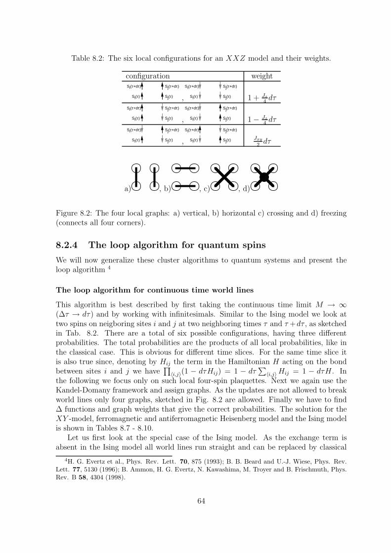
Table 8.2: The six local configurations for an XXZ model and their weights.
configuration weight
Si(τ)
Si(τ+dτ)
Sj(τ)
Sj(τ+dτ)
, Si(τ)
Si(τ+dτ)
Sj(τ)
Sj(τ+dτ)
1 + Jz
4dτ
Si(τ)
Si(τ+dτ)
Sj(τ)
Sj(τ+dτ)
, Si(τ)
Si(τ+dτ)
Sj(τ)
Sj(τ+dτ)
1− Jz
4dτ
Si(τ)
Si(τ+dτ)
Sj(τ)
Sj(τ+dτ)
, Si(τ)
Si(τ+dτ)
Sj(τ)
Sj(τ+dτ)
Jxy
2dτ
a) , b) , c) , d)
Figure 8.2: The four local graphs: a) vertical, b) horizontal c) crossing and d) freezing(connects all four corners).
8.2.4 The loop algorithm for quantum spins
We will now generalize these cluster algorithms to quantum systems and present theloop algorithm 4
The loop algorithm for continuous time world lines
This algorithm is best described by first taking the continuous time limit M → ∞(∆τ → dτ) and by working with infinitesimals. Similar to the Ising model we look attwo spins on neigboring sites i and j at two neighboring times τ and τ +dτ , as sketchedin Tab. 8.2. There are a total of six possible configurations, having three differentprobabilities. The total probabilities are the products of all local probabilities, like inthe classical case. This is obvious for different time slices. For the same time slice itis also true since, denoting by Hij the term in the Hamiltonian H acting on the bondbetween sites i and j we have
∏
〈i,j〉(1 − dτHij) = 1 − dτ∑
〈i,j〉Hij = 1 − dτH . Inthe following we focus only on such local four-spin plaquettes. Next we again use theKandel-Domany framework and assign graphs. As the updates are not allowed to breakworld lines only four graphs, sketched in Fig. 8.2 are allowed. Finally we have to find∆ functions and graph weights that give the correct probabilities. The solution for theXY -model, ferromagnetic and antiferromagnetic Heisenberg model and the Ising modelis shown in Tables 8.7 - 8.10.
Let us first look at the special case of the Ising model. As the exchange term isabsent in the Ising model all world lines run straight and can be replaced by classical
4H. G. Evertz et al., Phys. Rev. Lett. 70, 875 (1993); B. B. Beard and U.-J. Wiese, Phys. Rev.Lett. 77, 5130 (1996); B. Ammon, H. G. Evertz, N. Kawashima, M. Troyer and B. Frischmuth, Phys.Rev. B 58, 4304 (1998).
64
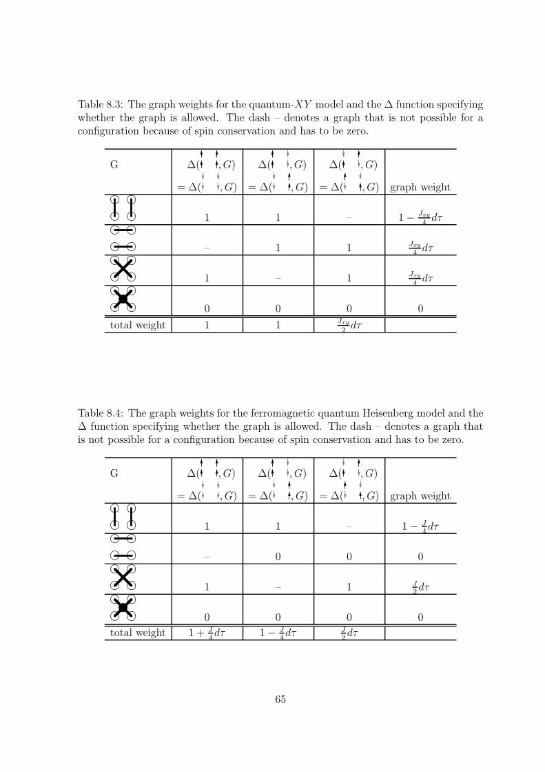
Table 8.3: The graph weights for the quantum-XY model and the ∆ function specifyingwhether the graph is allowed. The dash – denotes a graph that is not possible for aconfiguration because of spin conservation and has to be zero.
G ∆( , G) ∆( , G) ∆( , G)
= ∆( , G) = ∆( , G) = ∆( , G) graph weight
1 1 – 1− Jxy
4dτ
– 1 1 Jxy
4dτ
1 – 1 Jxy
4dτ
0 0 0 0
total weight 1 1 Jxy
2dτ
Table 8.4: The graph weights for the ferromagnetic quantum Heisenberg model and the∆ function specifying whether the graph is allowed. The dash – denotes a graph thatis not possible for a configuration because of spin conservation and has to be zero.
G ∆( , G) ∆( , G) ∆( , G)
= ∆( , G) = ∆( , G) = ∆( , G) graph weight
1 1 – 1− J4dτ
– 0 0 0
1 – 1 J2dτ
0 0 0 0
total weight 1 + J4dτ 1− J
4dτ J
2dτ
65
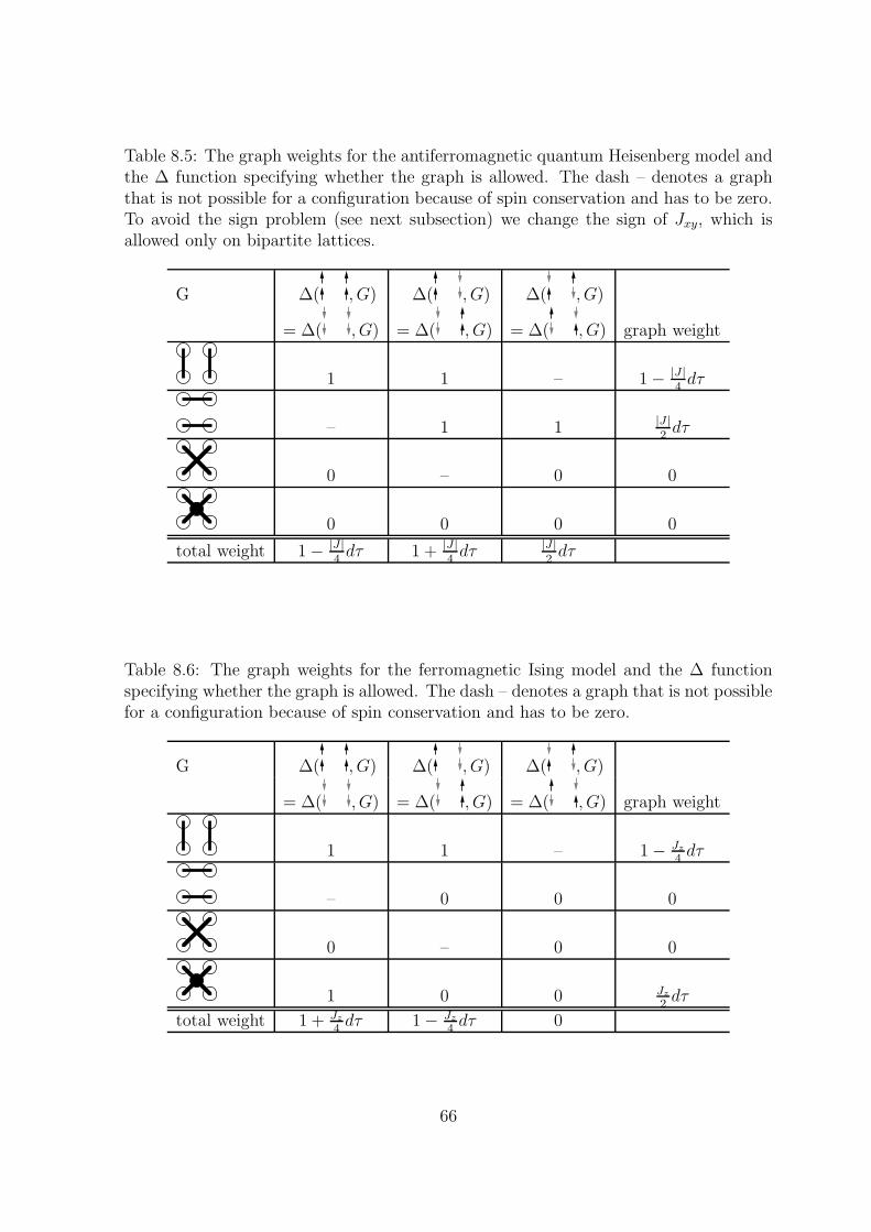
Table 8.5: The graph weights for the antiferromagnetic quantum Heisenberg model andthe ∆ function specifying whether the graph is allowed. The dash – denotes a graphthat is not possible for a configuration because of spin conservation and has to be zero.To avoid the sign problem (see next subsection) we change the sign of Jxy, which isallowed only on bipartite lattices.
G ∆( , G) ∆( , G) ∆( , G)
= ∆( , G) = ∆( , G) = ∆( , G) graph weight
1 1 – 1− |J |4dτ
– 1 1 |J |2dτ
0 – 0 0
0 0 0 0
total weight 1− |J |4dτ 1 + |J |
4dτ |J |
2dτ
Table 8.6: The graph weights for the ferromagnetic Ising model and the ∆ functionspecifying whether the graph is allowed. The dash – denotes a graph that is not possiblefor a configuration because of spin conservation and has to be zero.
G ∆( , G) ∆( , G) ∆( , G)
= ∆( , G) = ∆( , G) = ∆( , G) graph weight
1 1 – 1− Jz
4dτ
– 0 0 0
0 – 0 0
1 0 0 Jz
2dτ
total weight 1 + Jz
4dτ 1− Jz
4dτ 0
66
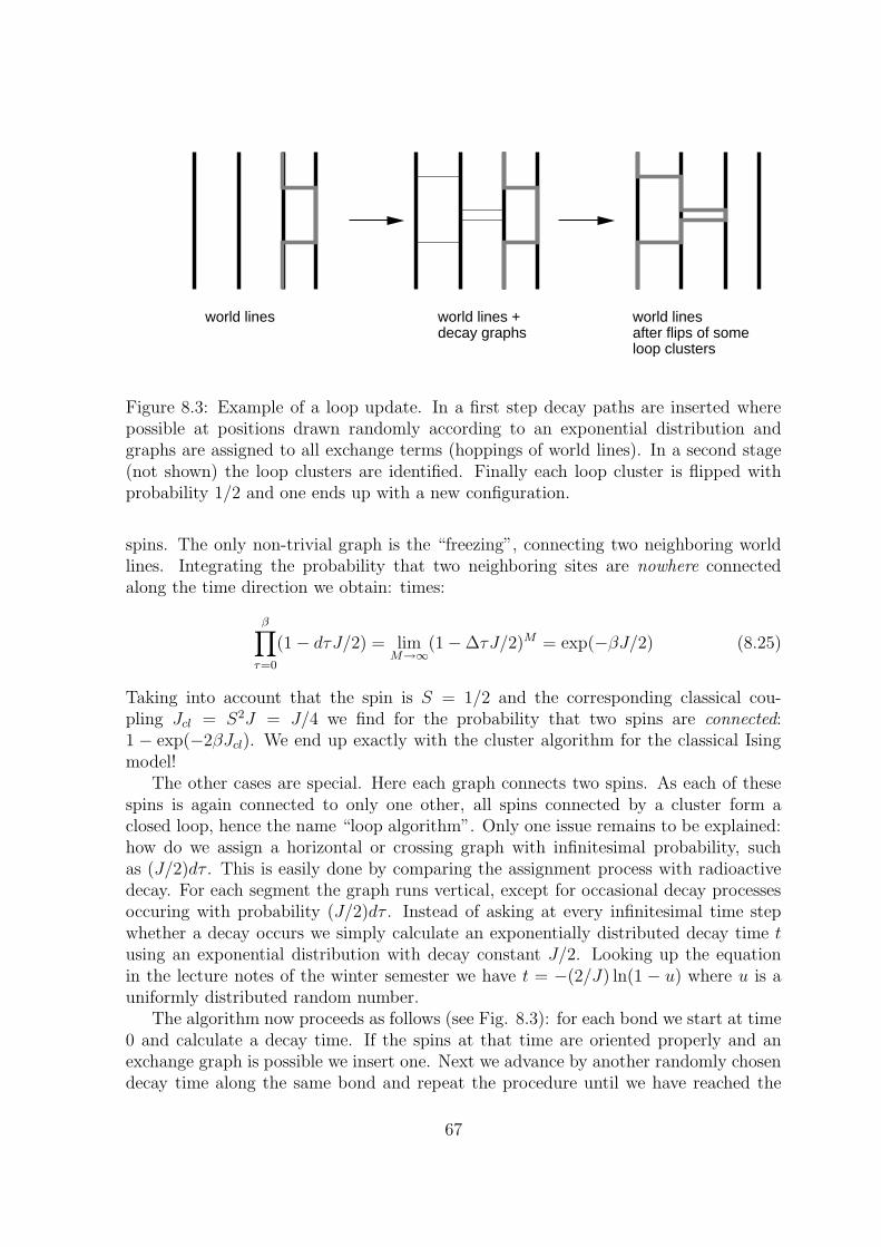
world lines world lines + decay graphs
world linesafter flips of some loop clusters
Figure 8.3: Example of a loop update. In a first step decay paths are inserted wherepossible at positions drawn randomly according to an exponential distribution andgraphs are assigned to all exchange terms (hoppings of world lines). In a second stage(not shown) the loop clusters are identified. Finally each loop cluster is flipped withprobability 1/2 and one ends up with a new configuration.
spins. The only non-trivial graph is the “freezing”, connecting two neighboring worldlines. Integrating the probability that two neighboring sites are nowhere connectedalong the time direction we obtain: times:
β∏
τ=0
(1− dτJ/2) = limM→∞
(1−∆τJ/2)M = exp(−βJ/2) (8.25)
Taking into account that the spin is S = 1/2 and the corresponding classical cou-pling Jcl = S2J = J/4 we find for the probability that two spins are connected:1 − exp(−2βJcl). We end up exactly with the cluster algorithm for the classical Isingmodel!
The other cases are special. Here each graph connects two spins. As each of thesespins is again connected to only one other, all spins connected by a cluster form aclosed loop, hence the name “loop algorithm”. Only one issue remains to be explained:how do we assign a horizontal or crossing graph with infinitesimal probability, suchas (J/2)dτ . This is easily done by comparing the assignment process with radioactivedecay. For each segment the graph runs vertical, except for occasional decay processesoccuring with probability (J/2)dτ . Instead of asking at every infinitesimal time stepwhether a decay occurs we simply calculate an exponentially distributed decay time tusing an exponential distribution with decay constant J/2. Looking up the equationin the lecture notes of the winter semester we have t = −(2/J) ln(1 − u) where u is auniformly distributed random number.
The algorithm now proceeds as follows (see Fig. 8.3): for each bond we start at time0 and calculate a decay time. If the spins at that time are oriented properly and anexchange graph is possible we insert one. Next we advance by another randomly chosendecay time along the same bond and repeat the procedure until we have reached the
67
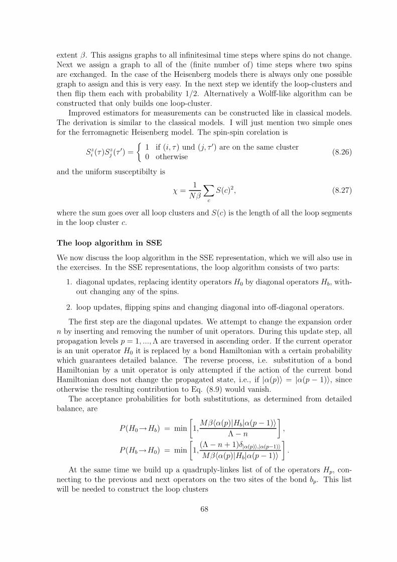
extent β. This assigns graphs to all infinitesimal time steps where spins do not change.Next we assign a graph to all of the (finite number of) time steps where two spinsare exchanged. In the case of the Heisenberg models there is always only one possiblegraph to assign and this is very easy. In the next step we identify the loop-clusters andthen flip them each with probability 1/2. Alternatively a Wolff-like algorithm can beconstructed that only builds one loop-cluster.
Improved estimators for measurements can be constructed like in classical models.The derivation is similar to the classical models. I will just mention two simple onesfor the ferromagnetic Heisenberg model. The spin-spin corelation is
Szi (τ)Szj (τ′) =
{
1 if (i, τ) und (j, τ ′) are on the same cluster0 otherwise
(8.26)
and the uniform susceptibilty is
χ =1
Nβ
∑
c
S(c)2, (8.27)
where the sum goes over all loop clusters and S(c) is the length of all the loop segmentsin the loop cluster c.
The loop algorithm in SSE
We now discuss the loop algorithm in the SSE representation, which we will also use inthe exercises. In the SSE representations, the loop algorithm consists of two parts:
1. diagonal updates, replacing identity operators H0 by diagonal operators Hb, with-out changing any of the spins.
2. loop updates, flipping spins and changing diagonal into off-diagonal operators.
The first step are the diagonal updates. We attempt to change the expansion ordern by inserting and removing the number of unit operators. During this update step, allpropagation levels p = 1, ...,Λ are traversed in ascending order. If the current operatoris an unit operator H0 it is replaced by a bond Hamiltonian with a certain probabilitywhich guarantees detailed balance. The reverse process, i.e. substitution of a bondHamiltonian by a unit operator is only attempted if the action of the current bondHamiltonian does not change the propagated state, i.e., if |α(p)〉 = |α(p − 1)〉, sinceotherwise the resulting contribution to Eq. (8.9) would vanish.
The acceptance probabilities for both substitutions, as determined from detailedbalance, are
P (H0→Hb) = min
[
1,Mβ〈α(p)|Hb|α(p− 1)〉
Λ− n
]
,
P (Hb→H0) = min
[
1,(Λ− n + 1)δ|α(p)〉,|α(p−1)〉Mβ〈α(p)|Hb|α(p− 1)〉
]
.
At the same time we build up a quadruply-linkes list of of the operators Hp, con-necting to the previous and next operators on the two sites of the bond bp. This listwill be needed to construct the loop clusters
68
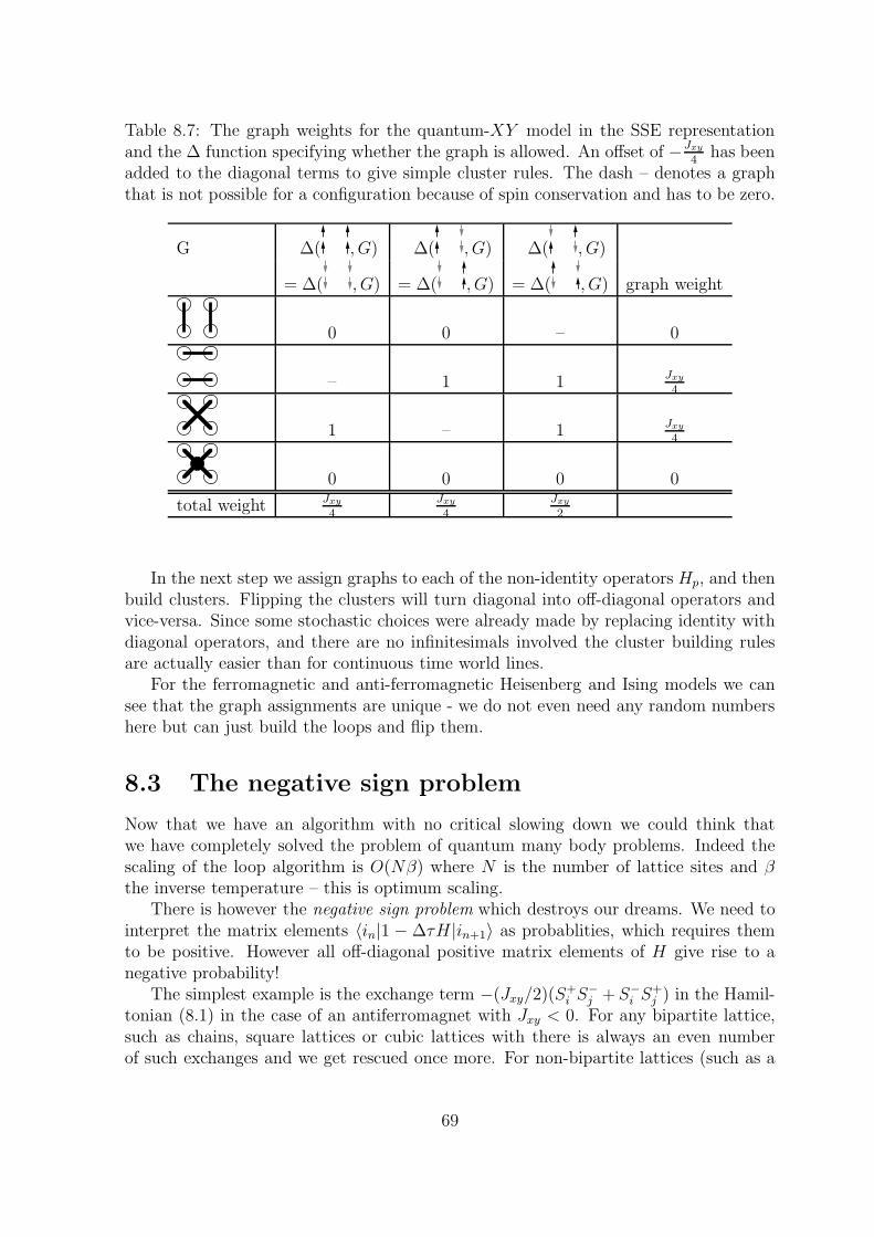
Table 8.7: The graph weights for the quantum-XY model in the SSE representationand the ∆ function specifying whether the graph is allowed. An offset of −Jxy
4has been
added to the diagonal terms to give simple cluster rules. The dash – denotes a graphthat is not possible for a configuration because of spin conservation and has to be zero.
G ∆( , G) ∆( , G) ∆( , G)
= ∆( , G) = ∆( , G) = ∆( , G) graph weight
0 0 – 0
– 1 1 Jxy
4
1 – 1 Jxy
4
0 0 0 0
total weight Jxy
4Jxy
4Jxy
2
In the next step we assign graphs to each of the non-identity operators Hp, and thenbuild clusters. Flipping the clusters will turn diagonal into off-diagonal operators andvice-versa. Since some stochastic choices were already made by replacing identity withdiagonal operators, and there are no infinitesimals involved the cluster building rulesare actually easier than for continuous time world lines.
For the ferromagnetic and anti-ferromagnetic Heisenberg and Ising models we cansee that the graph assignments are unique - we do not even need any random numbershere but can just build the loops and flip them.
8.3 The negative sign problem
Now that we have an algorithm with no critical slowing down we could think thatwe have completely solved the problem of quantum many body problems. Indeed thescaling of the loop algorithm is O(Nβ) where N is the number of lattice sites and βthe inverse temperature – this is optimum scaling.
There is however the negative sign problem which destroys our dreams. We need tointerpret the matrix elements 〈in|1 − ∆τH|in+1〉 as probablities, which requires themto be positive. However all off-diagonal positive matrix elements of H give rise to anegative probability!
The simplest example is the exchange term −(Jxy/2)(S+i S−j + S−i S
+j ) in the Hamil-
tonian (8.1) in the case of an antiferromagnet with Jxy < 0. For any bipartite lattice,such as chains, square lattices or cubic lattices with there is always an even numberof such exchanges and we get rescued once more. For non-bipartite lattices (such as a
69
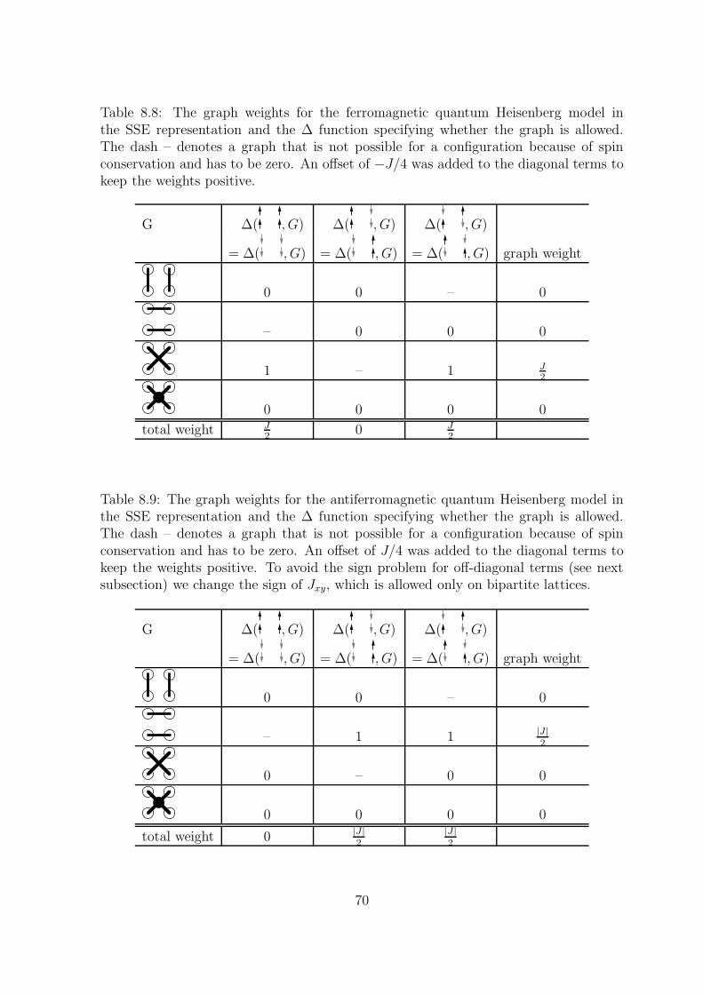
Table 8.8: The graph weights for the ferromagnetic quantum Heisenberg model inthe SSE representation and the ∆ function specifying whether the graph is allowed.The dash – denotes a graph that is not possible for a configuration because of spinconservation and has to be zero. An offset of −J/4 was added to the diagonal terms tokeep the weights positive.
G ∆( , G) ∆( , G) ∆( , G)
= ∆( , G) = ∆( , G) = ∆( , G) graph weight
0 0 – 0
– 0 0 0
1 – 1 J2
0 0 0 0
total weight J2
0 J2
Table 8.9: The graph weights for the antiferromagnetic quantum Heisenberg model inthe SSE representation and the ∆ function specifying whether the graph is allowed.The dash – denotes a graph that is not possible for a configuration because of spinconservation and has to be zero. An offset of J/4 was added to the diagonal terms tokeep the weights positive. To avoid the sign problem for off-diagonal terms (see nextsubsection) we change the sign of Jxy, which is allowed only on bipartite lattices.
G ∆( , G) ∆( , G) ∆( , G)
= ∆( , G) = ∆( , G) = ∆( , G) graph weight
0 0 – 0
– 1 1 |J |2
0 – 0 0
0 0 0 0
total weight 0 |J |2
|J |2
70
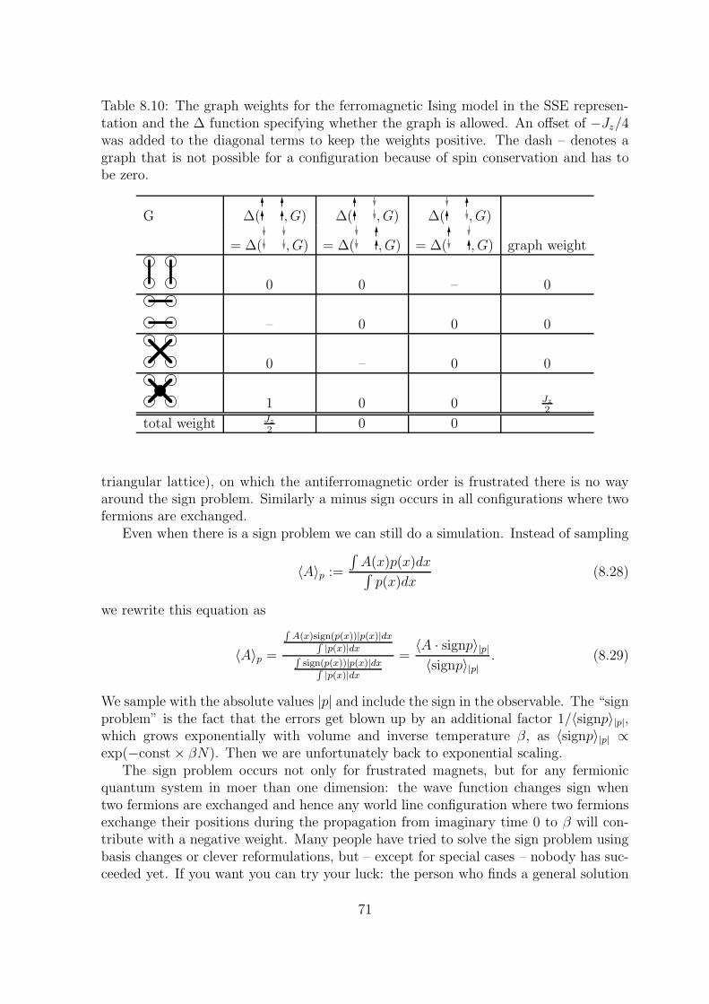
Table 8.10: The graph weights for the ferromagnetic Ising model in the SSE represen-tation and the ∆ function specifying whether the graph is allowed. An offset of −Jz/4was added to the diagonal terms to keep the weights positive. The dash – denotes agraph that is not possible for a configuration because of spin conservation and has tobe zero.
G ∆( , G) ∆( , G) ∆( , G)
= ∆( , G) = ∆( , G) = ∆( , G) graph weight
0 0 – 0
– 0 0 0
0 – 0 0
1 0 0 Jz
2
total weight Jz
20 0
triangular lattice), on which the antiferromagnetic order is frustrated there is no wayaround the sign problem. Similarly a minus sign occurs in all configurations where twofermions are exchanged.
Even when there is a sign problem we can still do a simulation. Instead of sampling
〈A〉p :=
∫
A(x)p(x)dx∫
p(x)dx(8.28)
we rewrite this equation as
〈A〉p =
R
A(x)sign(p(x))|p(x)|dxR
|p(x)|dxR
sign(p(x))|p(x)|dxR
|p(x)|dx
=〈A · signp〉|p|〈signp〉|p|
. (8.29)
We sample with the absolute values |p| and include the sign in the observable. The “signproblem” is the fact that the errors get blown up by an additional factor 1/〈signp〉|p|,which grows exponentially with volume and inverse temperature β, as 〈signp〉|p| ∝exp(−const × βN). Then we are unfortunately back to exponential scaling.
The sign problem occurs not only for frustrated magnets, but for any fermionicquantum system in moer than one dimension: the wave function changes sign whentwo fermions are exchanged and hence any world line configuration where two fermionsexchange their positions during the propagation from imaginary time 0 to β will con-tribute with a negative weight. Many people have tried to solve the sign problem usingbasis changes or clever reformulations, but – except for special cases – nobody has suc-ceeded yet. If you want you can try your luck: the person who finds a general solution
71
to the sign problem will surely get a Nobel Prize. Unfortunately it was recently shownthat the negative sign problem is NP-hard and thus almost certainly unsolvable in thegeneral case. 5
8.4 Worm and directed loop updates
The quantum loop algorithm, like the classical cluster algorithms work only for modelswith spin-inversion symmetry: a configuration of spins and the flipped configurationneed to have the same weight. Applying a magnetic field breaks this spin-inversionsymmetry, and the loop algorithm cannot be applied. For that case, Nikolay Prokof’evand coworkers invented the worm algorithm.6 The worm algorithm is based on a verysimple idea: while local updates on world lines are not ergodic (since knots cannot becreated or undone), the worm algorithm proceeds by cutting a world line, and thenmoves the open ends in local updates until they meet again and the world line is gluedtogether once more.
In the FS 2008, N. Prokof’ev will visit ETH and teach a course on the worm algo-rithms and related Monte Carlo methods. You are all invited to attend his lectures.
5M. Troyer and U.J. Wiese, Phys. Rev. Lett. 94, 170201 (2005).6N. V. Prokof’ev, B. V. Svistunov and I. S. Tupitsyn, Sov. Phys - JETP 87, 310 (1998).
72
Chapter 9
An Introduction to Quantum FieldTheory
9.1 Introduction
This chapter is a generalization of Sec. 5.6 on Path Integral Monte Carlo. Instead ofconsidering one (or N) quantum-mechanical particles as was done there, the idea isnow to consider a quantum field, which contains infinitely many degrees of freedom.However, in practice, we are going to simulate a large but finite number of degreesof freedom, and extrapolate at the end. So there really is not much difference withSec. 5.6.
The formal basis for Quantum Field Theory is an important subject, which will notbe covered here. The goal of this chapter is to convey some understanding of simulationsof quantum field theories, by appealing to intuition rather than rigor.
9.2 Path integrals: from classical mechanics to field
theory
Consider first the case of a single, classical particle with Hamiltonian H = p2
2m+ V .
Hamilton’s equations describe the time-evolution of this particle:
dq
dt= +
∂H
∂p−→ q =
p
m(9.1)
dp
dt= −∂H
∂q−→ p = −∇V (9.2)
The usual point of view is to start from initial conditions (q, q) at time t = 0, andevolve q and q according to the coupled ODEs above. Note, however, that the boundaryconditions can instead be split between the beginning and the end of the evolution. Inparticular, one can specify the beginning and ending coordinates (q(0), q(t)). Thereis a unique path q(t′), t′ ∈ [0, t], which satisfies the above equations, and specifies theinitial and final velocities. To find this path, it is convenient to change viewpoint andconsider the action S =
∫ t
0dt′L(q, q), where L is the Lagrangian 1
2mq2 − V (q). One
73
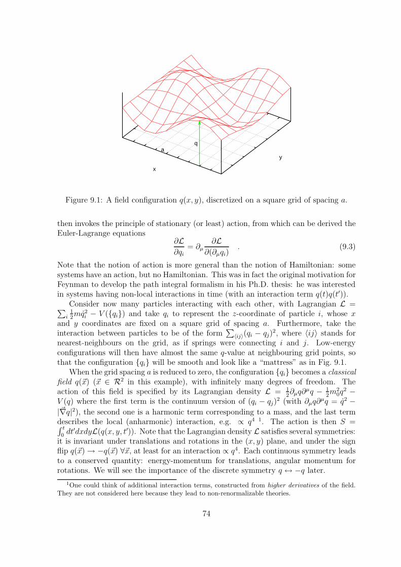
qa
x
y
Figure 9.1: A field configuration q(x, y), discretized on a square grid of spacing a.
then invokes the principle of stationary (or least) action, from which can be derived theEuler-Lagrange equations
∂L∂qi
= ∂µ∂L
∂(∂µqi). (9.3)
Note that the notion of action is more general than the notion of Hamiltonian: somesystems have an action, but no Hamiltonian. This was in fact the original motivation forFeynman to develop the path integral formalism in his Ph.D. thesis: he was interestedin systems having non-local interactions in time (with an interaction term q(t)q(t′)).
Consider now many particles interacting with each other, with Lagrangian L =∑
i12mq2
i − V ({qi}) and take qi to represent the z-coordinate of particle i, whose xand y coordinates are fixed on a square grid of spacing a. Furthermore, take theinteraction between particles to be of the form
∑
〈ij〉(qi − qj)2, where 〈ij〉 stands for
nearest-neighbours on the grid, as if springs were connecting i and j. Low-energyconfigurations will then have almost the same q-value at neighbouring grid points, sothat the configuration {qi} will be smooth and look like a “mattress” as in Fig. 9.1.
When the grid spacing a is reduced to zero, the configuration {qi} becomes a classicalfield q(~x) (~x ∈ R2 in this example), with infinitely many degrees of freedom. Theaction of this field is specified by its Lagrangian density L = 1
2∂µq∂
µq − 12m2
0q2 −
V (q) where the first term is the continuum version of (qi − qj)2 (with ∂µq∂µq = q2 −
|~∇q|2), the second one is a harmonic term corresponding to a mass, and the last termdescribes the local (anharmonic) interaction, e.g. ∝ q4 1. The action is then S =∫ t
0dt′dxdyL(q(x, y, t′)). Note that the Lagrangian density L satisfies several symmetries:
it is invariant under translations and rotations in the (x, y) plane, and under the signflip q(~x)→ −q(~x) ∀~x, at least for an interaction ∝ q4. Each continuous symmetry leadsto a conserved quantity: energy-momentum for translations, angular momentum forrotations. We will see the importance of the discrete symmetry q ↔ −q later.
1One could think of additional interaction terms, constructed from higher derivatives of the field.They are not considered here because they lead to non-renormalizable theories.
74
Now we can consider quantum effects on the above system. As a result of quantumfluctuations, the path from q(t = 0) to q(t) is no longer unique. All paths contribute,with an amplitude ∝ exp(− i
~
∫ t
0dt′L), from which it becomes clear that the magnitude
of relevant fluctuations in the action is ~. One can then follow the strategy of Sec. 5.6and make time purely imaginary, by introducing τ = −it ∈ R. The immediate result isthat −idt′ above becomes dτ ′, so that the amplitude becomes real. The other change isq2 → −(∂τq)
2, so that an overall minus sign can be taken out, leading to the amplitude
exp(−1
~SE) (9.4)
where SE =∫
dτ ′d~xLE is the Euclidean action, and
LE =1
2(∂µφ)2 +
1
2m2
0φ2 + V (φ) (9.5)
is the Euclidean Lagrangian density, and the field q is now denoted by φ as is customary.The first term (∂µφ)2 = (∂τφ)2 + |~∇φ|2 is now symmetric between space and time, sothat the metric is Euclidean in (d+1) dimensions (d spatial dimensions, plus Euclideantime).
It is worth summarizing the sign flips which occurred in the kinetic energy T andthe potential energy U during the successive steps we have just taken. We started withthe Hamiltonian H = T + U , then considered the Lagrangian L = T − U . Going toimaginary time changes the sign of T . Finally, we take out an overall minus sign in thedefinition of LE , so that paths with the smallest action are the most likely. This leadsto the Euclidean Lagrangian density LE = T +U , which is identical to the Hamiltonianwe started from, except that the momentum p is replaced by the derivative ∂0φ.
It is also useful to perform some elementary dimensional analysis. Since it appearsin the exponent of the amplitude Eq.(9.4), the Euclidean action SE is dimensionless (weset ~ = 1). Hence the Euclidean Lagrangian density has mass dimension (d + 1), andtherefore the field φ has mass dimension d−1
2. This is interesting, because if we take the
“normal” number of spatial dimensions d = 3 and the interaction term V (φ) = g04!φ4,
then g0 is a dimensionless number. It makes sense then to perform a Taylor expansion ofthis theory in powers of g0 about the free case g0 = 0: this is the scope of perturbationtheory. Here, we will try to obtain non-perturbative results, by directly simulating thetheory at some finite, large value of g0.
We have so far considered a field φ(~x, τ) which takes values in R. It is easy togeneralize the Lagrangian density Eq.(9.5) to cases when φ takes values in C, or has
several components forming a vector ~φ ≡
φ1
..φN
, perhaps with a constraint∑
N φ2k =
1, depending on the desired symmetries. Typically, the Euclidean Lagrangian densityis the starting, defining point of a quantum field theory.
Finally, we can introduce a finite temperature T , exactly as we did in the quantum-mechanical case: we make the Euclidean time direction compact: τ ∈ [0, β = 1
T], and
impose periodic boundary conditions on the field φ: φ(~x, β) = φ(~x, 0) ∀~x. This worksfor the same reason as in quantum mechanics: the partition function
Z =
∫
periodic
Dφ exp(−∫ β
0
dτ ′d~xLE(φ)) (9.6)
75
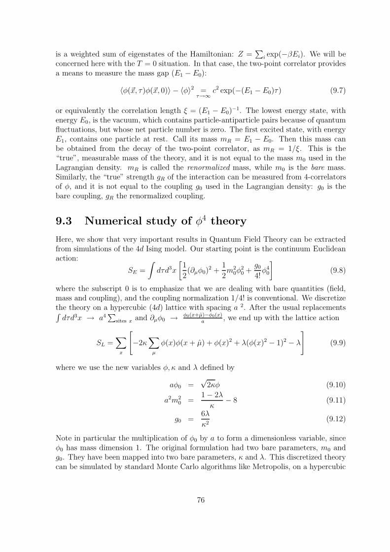
is a weighted sum of eigenstates of the Hamiltonian: Z =∑
i exp(−βEi). We will beconcerned here with the T = 0 situation. In that case, the two-point correlator providesa means to measure the mass gap (E1 − E0):
〈φ(~x, τ)φ(~x, 0)〉 − 〈φ〉2 =τ→∞
c2 exp(−(E1 −E0)τ) (9.7)
or equivalently the correlation length ξ = (E1 − E0)−1. The lowest energy state, with
energy E0, is the vacuum, which contains particle-antiparticle pairs because of quantumfluctuations, but whose net particle number is zero. The first excited state, with energyE1, contains one particle at rest. Call its mass mR = E1 − E0. Then this mass canbe obtained from the decay of the two-point correlator, as mR = 1/ξ. This is the“true”, measurable mass of the theory, and it is not equal to the mass m0 used in theLagrangian density. mR is called the renormalized mass, while m0 is the bare mass.Similarly, the “true” strength gR of the interaction can be measured from 4-correlatorsof φ, and it is not equal to the coupling g0 used in the Lagrangian density: g0 is thebare coupling, gR the renormalized coupling.
9.3 Numerical study of φ4 theory
Here, we show that very important results in Quantum Field Theory can be extractedfrom simulations of the 4d Ising model. Our starting point is the continuum Euclideanaction:
SE =
∫
dτd3x
[
1
2(∂µφ0)
2 +1
2m2
0φ20 +
g0
4!φ4
0
]
(9.8)
where the subscript 0 is to emphasize that we are dealing with bare quantities (field,mass and coupling), and the coupling normalization 1/4! is conventional. We discretizethe theory on a hypercubic (4d) lattice with spacing a 2. After the usual replacements∫
dτd3x → a4∑
sites x and ∂µφ0 → φ0(x+µ)−φ0(x)a
, we end up with the lattice action
SL =∑
x
[
−2κ∑
µ
φ(x)φ(x+ µ) + φ(x)2 + λ(φ(x)2 − 1)2 − λ]
(9.9)
where we use the new variables φ, κ and λ defined by
aφ0 =√
2κφ (9.10)
a2m20 =
1− 2λ
κ− 8 (9.11)
g0 =6λ
κ2(9.12)
Note in particular the multiplication of φ0 by a to form a dimensionless variable, sinceφ0 has mass dimension 1. The original formulation had two bare parameters, m0 andg0. They have been mapped into two bare parameters, κ and λ. This discretized theorycan be simulated by standard Monte Carlo algorithms like Metropolis, on a hypercubic
76
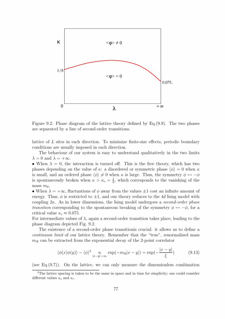
φ> = 0<
φ> = 0<
/
0 8
+
1/8
0.075..
λ
κ
Figure 9.2: Phase diagram of the lattice theory defined by Eq.(9.9). The two phasesare separated by a line of second-order transitions.
lattice of L sites in each direction. To minimize finite-size effects, periodic boundaryconditions are usually imposed in each direction.
The behaviour of our system is easy to understand qualitatively in the two limitsλ = 0 and λ = +∞.• When λ = 0, the interaction is turned off. This is the free theory, which has twophases depending on the value of κ: a disordered or symmetric phase 〈φ〉 = 0 when κis small, and an ordered phase 〈φ〉 6= 0 when κ is large. Thus, the symmetry φ ↔ −φis spontaneously broken when κ > κc = 1
8, which corresponds to the vanishing of the
mass m0.• When λ = +∞, fluctuations of φ away from the values ±1 cost an infinite amount ofenergy. Thus, φ is restricted to ±1, and our theory reduces to the 4d Ising model withcoupling 2κ. As in lower dimensions, the Ising model undergoes a second-order phasetransition corresponding to the spontaneous breaking of the symmetry φ ↔ −φ, for acritical value κc ≈ 0.075.For intermediate values of λ, again a second-order transition takes place, leading to thephase diagram depicted Fig. 9.2.
The existence of a second-order phase transitionis crucial: it allows us to define acontinuum limit of our lattice theory. Remember that the “true”, renormalized massmR can be extracted from the exponential decay of the 2-point correlator
〈φ(x)φ(y)〉 − 〈φ〉2 ∝|x−y|→∞
exp(−mR|x− y|) = exp(−|x− y|ξ
) (9.13)
(see Eq.(9.7)). On the lattice, we can only measure the dimensionless combination
2The lattice spacing is taken to be the same in space and in time for simplicity; one could considerdifferent values as and aτ .
77
ξa
diverges,fixed,a ξ grows ξa
divergesfixed,ξ a shrinks
ξ
ξ
ξa
a
a
a
ξ
2nd order P.T. 2nd order P.T.
Solid State QFT
Figure 9.3: Two different viewpoints on a second-order phase transition: in solid-statephysics (left), the crystal is “real” and the physical correlation length diverges; in quan-tum field theory (right), the correlation length is “real”, and the lattice spacing shrinksto zero.
amR = 1ξ/a
, and the separation |x− y| can only be measured in lattice units, i.e. |x−y|a
.
Taking the continuum limit a→ 0 (while keeping mR fixed) forces the correlation lengthmeasured in lattice units, i.e. ξ/a, to diverge. This only occurs when the lattice theoryhas a second-order phase transition (or higher order).
Therefore, the interpretation of a second-order phase transition is different betweensolid-state physics and lattice field theory. In the first case, the lattice spacing has aphysical meaning, like the distance between two ions in a crystal: the lattice is “forreal”, and the correlation length really diverges at a second-order critical point. In thelattice field theory, the correlation length is “for real”, and the lattice spacing a shrinksto zero at the critical point. This is illustrated in Fig. 9.3.
In this latter case, one must be careful that the physical box size (La) also shrinksas a→ 0. In order to obtain a controlled continuum limit at constant physical volume,one must increase the number of lattice points L in each direction keeping (La) fixed.
Going back to our φ4 theory, one sees that a continuum limit can be defined forany value of the bare coupling λ ∈ [0,+∞], by tuning κ to its critical value κc(λ).An interesting question is: what is the value of the “true”, renormalized coupling as afunction of λ ? The answer is clear when λ = 0: the theory is free, and the coupling is
78
zero, whether bare or renormalized. To obtain a non-zero answer, a reasonable strategyis to maximize the bare coupling, and thus to consider the Ising limit λ = +∞. Therenormalized coupling is extracted from the strength of the 4-spin correlation, normal-ized as explained in Exercise 10. The rather surprising answer is that the renormalizedcoupling is zero, just like for λ = 0. In fact, the renormalized coupling is always zero forany choice of λ. In other words, the renormalized φ4 theory is free, no matter the valueof the bare coupling! The formal statement is that the φ4 theory is “trivial”. Note thatthis is only true in (3 + 1) dimensions. In lower dimensions, the renormalized couplingis non-zero.
Now, why is this finding important? The Standard Model of particle interactionscontains a Higgs particle, which gives a mass to all other particles by coupling to them.The field theory describing the Higgs particle is very much like the φ4 theory we have
just studied, except that the field φ is now a complex doublet
(
φ1 + iφ2
φ3 + iφ4
)
. The bare
parameters are chosen so that the system is in the broken-symmetry phase, where φhas a non-zero expectation value. The masses of all particles are proportional to 〈φ〉,therefore it is crucial that 〈φ〉 6= 0. In turn, this symmetry breaking is only possible ifthe coupling λ is non-zero. But, as we have seen, the “true”, renormalized value of λ iszero. Therefore, we have a logical inconsistency. The consequence is that the StandardModel cannot be the final, exact description of particle interactions. Some new physicsbeyond the Standard Model must exist, and from the numerical study of the latticetheory near κc(λ), one can set the energy scale for this new physics to become visible ataround 600-800 GeV. This argument is so powerful that it has been used in the designof the Large Hadron Collider (LHC), to be turned on at CERN within a year, andwhich will study collisions up to about 1000 GeV only.
9.4 Gauge theories
Of the four forces known in Nature, at least three (the strong, the weak and the electro-magnetic forces) are described by gauge theories. In addition to the usual “matter” fields(electrons, quarks), these theories contain “gauge” fields (photons, W and Z bosons,gluons) which “mediate” the interaction: the interaction between, say, two electrons iscaused by the exchange of photons between them. This is analogous to the exchangeof momentum which occurs when one person throws a ball at another, and the othercatches it. In this way, two particles interact when they are far apart, even thoughthe Lagrangian contains only local interactions. Moreover, gauge theories are invariantunder a larger class of symmetries, namely local (x-dependent) symmetries.
9.4.1 QED
As an example, let us consider here a variant of Quantum ElectroDynamics (QED),called scalar QED, where electrons are turned into bosons. A simple modification ofthe previous φ4 theory is required: in order to represent charged bosons, the field φ,instead of being real, is made complex, φ(x) ∈ C. The continuum Euclidean action
79
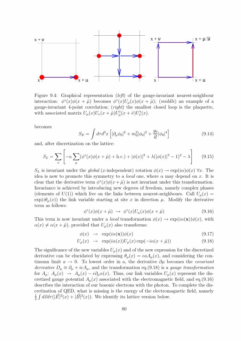
µx x +
x + ν µ + ν
x x +
x +x + ν
µ
Figure 9.4: Graphical representation (left) of the gauge-invariant nearest-neighbourinteraction: φ∗(x)φ(x + µ) becomes φ∗(x)Uµ(x)φ(x + µ); (middle) an example of agauge-invariant 4-point correlation; (right) the smallest closed loop is the plaquette,with associated matrix Uµ(x)Uν(x+ µ)U †µ(x+ ν)U †ν(x).
becomes
SE =
∫
dτd3x[
|∂µφ0|2 +m20|φ0|2 +
g0
4!|φ0|4
]
(9.14)
and, after discretization on the lattice:
SL =∑
x
[
−κ∑
µ
(φ∗(x)φ(x+ µ) + h.c.) + |φ(x)|2 + λ(|φ(x)|2 − 1)2 − λ]
(9.15)
SL is invariant under the global (x-independent) rotation φ(x)→ exp(iα)φ(x) ∀x. Theidea is now to promote this symmetry to a local one, where α may depend on x. It isclear that the derivative term φ∗(x)φ(x+ µ) is not invariant under this transformation.Invariance is achieved by introducing new degrees of freedom, namely complex phases(elements of U(1)) which live on the links between nearest-neighbours. Call Uµ(x) =exp(iθµ(x)) the link variable starting at site x in direction µ. Modify the derivativeterm as follows:
φ∗(x)φ(x+ µ) → φ∗(x)Uµ(x)φ(x+ µ) (9.16)
This term is now invariant under a local transformation φ(x) → exp(iα(x))φ(x), withα(x) 6= α(x+ µ), provided that Uµ(x) also transforms:
φ(x) → exp(iα(x))φ(x) (9.17)
Uµ(x) → exp(iα(x))Uµ(x) exp(−iα(x+ µ)) (9.18)
The significance of the new variables Uµ(x) and of the new expression for the discretizedderivative can be elucidated by expressing θµ(x) = eaAµ(x), and considering the con-tinuum limit a → 0. To lowest order in a, the derivative ∂µ becomes the covariantderivative Dµ ≡ ∂µ + ieAµ, and the transformation eq.(9.18) is a gauge transformationfor Aµ: Aµ(x) → Aµ(x) − e∂µα(x). Thus, our link variables Uµ(x) represent the dis-cretized gauge potential Aµ(x) associated with the electromagnetic field, and eq.(9.16)describes the interaction of our bosonic electrons with the photon. To complete the dis-cretization of QED, what is missing is the energy of the electromagnetic field, namely12
∫
d~xdτ(| ~E|2(x) + | ~B|2(x)). We identify its lattice version below.
80
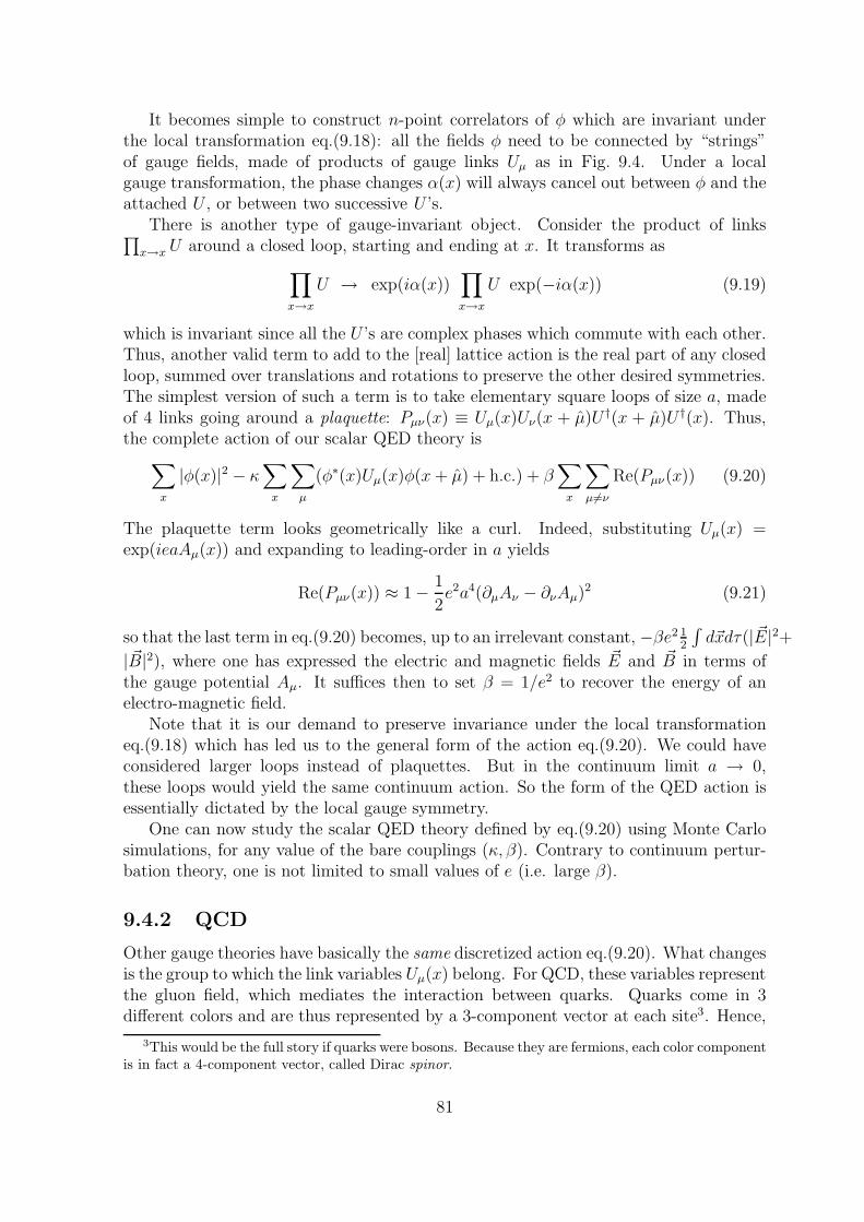
It becomes simple to construct n-point correlators of φ which are invariant underthe local transformation eq.(9.18): all the fields φ need to be connected by “strings”of gauge fields, made of products of gauge links Uµ as in Fig. 9.4. Under a localgauge transformation, the phase changes α(x) will always cancel out between φ and theattached U , or between two successive U ’s.
There is another type of gauge-invariant object. Consider the product of links∏
x→x U around a closed loop, starting and ending at x. It transforms as
∏
x→xU → exp(iα(x))
∏
x→xU exp(−iα(x)) (9.19)
which is invariant since all the U ’s are complex phases which commute with each other.Thus, another valid term to add to the [real] lattice action is the real part of any closedloop, summed over translations and rotations to preserve the other desired symmetries.The simplest version of such a term is to take elementary square loops of size a, madeof 4 links going around a plaquette: Pµν(x) ≡ Uµ(x)Uν(x + µ)U †(x + µ)U †(x). Thus,the complete action of our scalar QED theory is
∑
x
|φ(x)|2 − κ∑
x
∑
µ
(φ∗(x)Uµ(x)φ(x+ µ) + h.c.) + β∑
x
∑
µ6=νRe(Pµν(x)) (9.20)
The plaquette term looks geometrically like a curl. Indeed, substituting Uµ(x) =exp(ieaAµ(x)) and expanding to leading-order in a yields
Re(Pµν(x)) ≈ 1− 1
2e2a4(∂µAν − ∂νAµ)2 (9.21)
so that the last term in eq.(9.20) becomes, up to an irrelevant constant, −βe2 12
∫
d~xdτ(| ~E|2+| ~B|2), where one has expressed the electric and magnetic fields ~E and ~B in terms ofthe gauge potential Aµ. It suffices then to set β = 1/e2 to recover the energy of anelectro-magnetic field.
Note that it is our demand to preserve invariance under the local transformationeq.(9.18) which has led us to the general form of the action eq.(9.20). We could haveconsidered larger loops instead of plaquettes. But in the continuum limit a → 0,these loops would yield the same continuum action. So the form of the QED action isessentially dictated by the local gauge symmetry.
One can now study the scalar QED theory defined by eq.(9.20) using Monte Carlosimulations, for any value of the bare couplings (κ, β). Contrary to continuum pertur-bation theory, one is not limited to small values of e (i.e. large β).
9.4.2 QCD
Other gauge theories have basically the same discretized action eq.(9.20). What changesis the group to which the link variables Uµ(x) belong. For QCD, these variables representthe gluon field, which mediates the interaction between quarks. Quarks come in 3different colors and are thus represented by a 3-component vector at each site3. Hence,
3This would be the full story if quarks were bosons. Because they are fermions, each color componentis in fact a 4-component vector, called Dirac spinor.
81
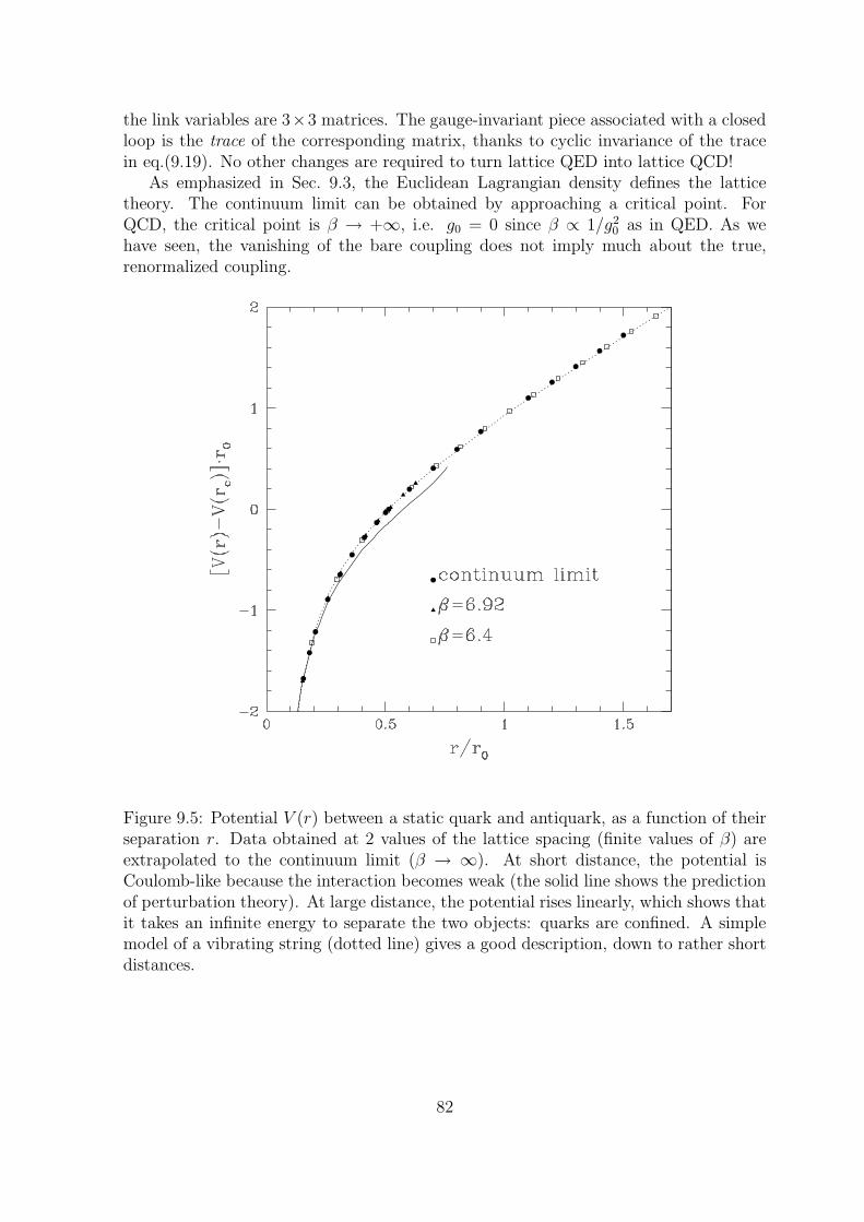
the link variables are 3×3 matrices. The gauge-invariant piece associated with a closedloop is the trace of the corresponding matrix, thanks to cyclic invariance of the tracein eq.(9.19). No other changes are required to turn lattice QED into lattice QCD!
As emphasized in Sec. 9.3, the Euclidean Lagrangian density defines the latticetheory. The continuum limit can be obtained by approaching a critical point. ForQCD, the critical point is β → +∞, i.e. g0 = 0 since β ∝ 1/g2
0 as in QED. As wehave seen, the vanishing of the bare coupling does not imply much about the true,renormalized coupling.
Figure 9.5: Potential V (r) between a static quark and antiquark, as a function of theirseparation r. Data obtained at 2 values of the lattice spacing (finite values of β) areextrapolated to the continuum limit (β → ∞). At short distance, the potential isCoulomb-like because the interaction becomes weak (the solid line shows the predictionof perturbation theory). At large distance, the potential rises linearly, which shows thatit takes an infinite energy to separate the two objects: quarks are confined. A simplemodel of a vibrating string (dotted line) gives a good description, down to rather shortdistances.
82
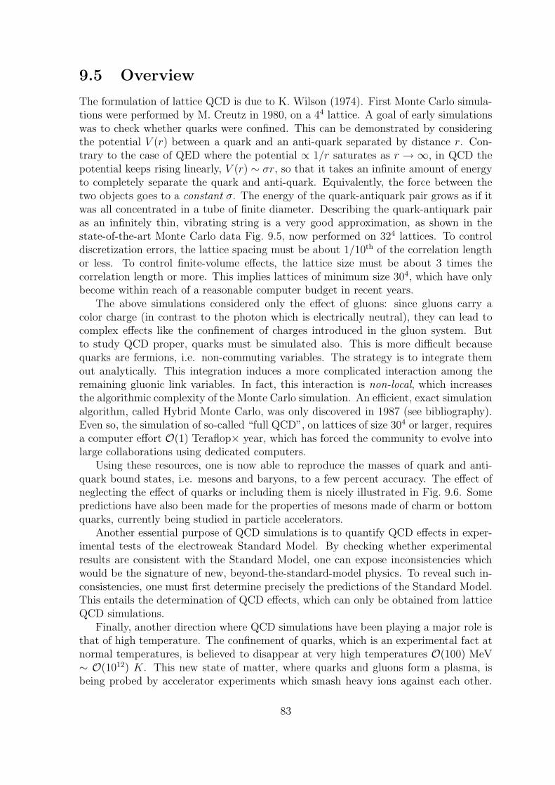
9.5 Overview
The formulation of lattice QCD is due to K. Wilson (1974). First Monte Carlo simula-tions were performed by M. Creutz in 1980, on a 44 lattice. A goal of early simulationswas to check whether quarks were confined. This can be demonstrated by consideringthe potential V (r) between a quark and an anti-quark separated by distance r. Con-trary to the case of QED where the potential ∝ 1/r saturates as r → ∞, in QCD thepotential keeps rising linearly, V (r) ∼ σr, so that it takes an infinite amount of energyto completely separate the quark and anti-quark. Equivalently, the force between thetwo objects goes to a constant σ. The energy of the quark-antiquark pair grows as if itwas all concentrated in a tube of finite diameter. Describing the quark-antiquark pairas an infinitely thin, vibrating string is a very good approximation, as shown in thestate-of-the-art Monte Carlo data Fig. 9.5, now performed on 324 lattices. To controldiscretization errors, the lattice spacing must be about 1/10th of the correlation lengthor less. To control finite-volume effects, the lattice size must be about 3 times thecorrelation length or more. This implies lattices of minimum size 304, which have onlybecome within reach of a reasonable computer budget in recent years.
The above simulations considered only the effect of gluons: since gluons carry acolor charge (in contrast to the photon which is electrically neutral), they can lead tocomplex effects like the confinement of charges introduced in the gluon system. Butto study QCD proper, quarks must be simulated also. This is more difficult becausequarks are fermions, i.e. non-commuting variables. The strategy is to integrate themout analytically. This integration induces a more complicated interaction among theremaining gluonic link variables. In fact, this interaction is non-local, which increasesthe algorithmic complexity of the Monte Carlo simulation. An efficient, exact simulationalgorithm, called Hybrid Monte Carlo, was only discovered in 1987 (see bibliography).Even so, the simulation of so-called “full QCD”, on lattices of size 304 or larger, requiresa computer effort O(1) Teraflop× year, which has forced the community to evolve intolarge collaborations using dedicated computers.
Using these resources, one is now able to reproduce the masses of quark and anti-quark bound states, i.e. mesons and baryons, to a few percent accuracy. The effect ofneglecting the effect of quarks or including them is nicely illustrated in Fig. 9.6. Somepredictions have also been made for the properties of mesons made of charm or bottomquarks, currently being studied in particle accelerators.
Another essential purpose of QCD simulations is to quantify QCD effects in exper-imental tests of the electroweak Standard Model. By checking whether experimentalresults are consistent with the Standard Model, one can expose inconsistencies whichwould be the signature of new, beyond-the-standard-model physics. To reveal such in-consistencies, one must first determine precisely the predictions of the Standard Model.This entails the determination of QCD effects, which can only be obtained from latticeQCD simulations.
Finally, another direction where QCD simulations have been playing a major role isthat of high temperature. The confinement of quarks, which is an experimental fact atnormal temperatures, is believed to disappear at very high temperatures O(100) MeV∼ O(1012) K. This new state of matter, where quarks and gluons form a plasma, isbeing probed by accelerator experiments which smash heavy ions against each other.
83
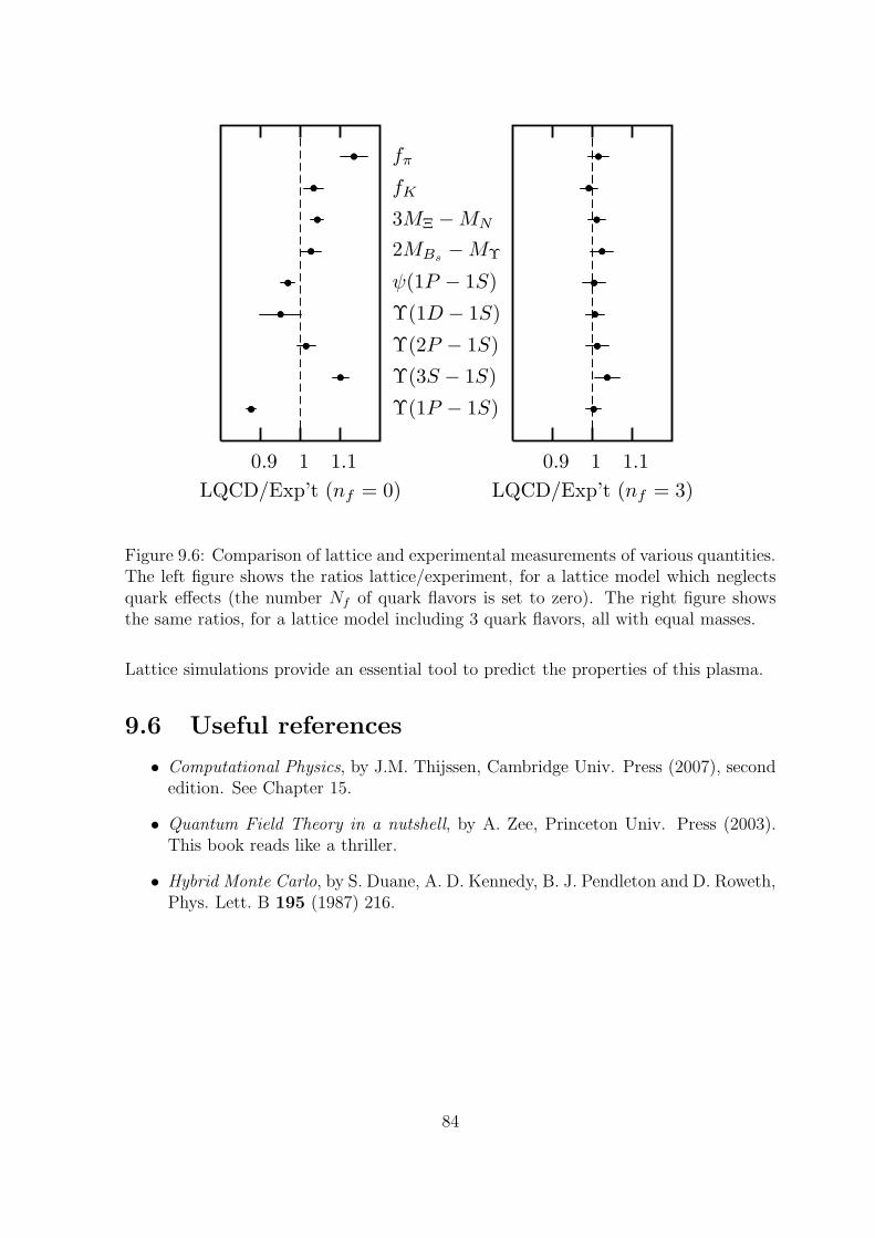
fπ
fK
3MΞ −MN
2MBs−MΥ
ψ(1P − 1S)
Υ(1D − 1S)
Υ(2P − 1S)
Υ(3S − 1S)
Υ(1P − 1S)
LQCD/Exp’t (nf = 0)
1.110.9
LQCD/Exp’t (nf = 3)
1.110.9
Figure 9.6: Comparison of lattice and experimental measurements of various quantities.The left figure shows the ratios lattice/experiment, for a lattice model which neglectsquark effects (the number Nf of quark flavors is set to zero). The right figure showsthe same ratios, for a lattice model including 3 quark flavors, all with equal masses.
Lattice simulations provide an essential tool to predict the properties of this plasma.
9.6 Useful references
• Computational Physics, by J.M. Thijssen, Cambridge Univ. Press (2007), secondedition. See Chapter 15.
• Quantum Field Theory in a nutshell, by A. Zee, Princeton Univ. Press (2003).This book reads like a thriller.
• Hybrid Monte Carlo, by S. Duane, A. D. Kennedy, B. J. Pendleton and D. Roweth,Phys. Lett. B 195 (1987) 216.
84
Appendix A
Numerical methods
A.1 Numerical root solvers
The purpose of a root solver is to find a solution (a root) to the equation
f(x) = 0, (A.1)
or in general to a multi-dimensional equation
~f(~x) = 0. (A.2)
Numerical root solvers should be well known from the numerics courses and we willjust review three simple root solvers here. Keep in mind that in any serious calculationit is usually best to use a well optimized and tested library function over a hand-codedroot solver.
A.1.1 The Newton and secant methods
The Newton method is one of best known root solvers, however it is not guaranteed toconverge. The key idea is to start from a guess x0, linearize the equation around thatguess
f(x0) + (x− x0)f′(x0) = 0 (A.3)
and solve this linearized equation to obtain a better estimate x1. Iterating this procedurewe obtain the Newton method:
xn+1 = xn −f(xn)
f ′(xn). (A.4)
If the derivative f ′ is not known analytically, as is the case in our shooting problems,we can estimate it from the difference of the last two points:
f ′(xn) ≈f(xn)− f(xn−1)
xn − xn−1(A.5)
Substituting this into the Newton method (A.4) we obtain the secant method:
xn+1 = xn − (xn − xn−1)f(xn)
f(xn)− f(xn−1). (A.6)
a
The Newton method can easily be generalized to higher dimensional equations, bydefining the matrix of derivatives
Aij(~x) =∂fi(~x)
∂xj(A.7)
to obtain the higher dimensional Newton method
~xn+1 = ~xn − A−1 ~f(~x) (A.8)
If the derivatives Aij(~x) are not known analytically they can be estimated through finitedifferences:
Aij(~x) =fi(~x+ hj~ej)− fi(~x)
hjwith hj ≈ xj
√ε (A.9)
where ε is the machine precision (about 10−16 for double precision floating point num-bers on most machines).
A.1.2 The bisection method and regula falsi
Both the bisection method and the regula falsi require two starting values x0 and x1
surrounding the root, with f(x0) < 0 and f(x1) > 0 so that under the assumption of acontinuous function f there exists at least one root between x0 and x1.
The bisection method performs the following iteration
1. define a mid-point xm = (x0 + x1)/2.
2. if signf(xm) = signf(x0) replace x0 ← xm otherwise replace x1 ← xm
until a root is found.The regula falsi works in a similar fashion:
1. estimate the function f by a straight line from x0 to x1 and calculate the root ofthis linearized function: x2 = (f(x0)x1 − f(x1)x0)/(f(x1)− f(x0)
2. if signf(x2) = signf(x0) replace x0 ← x2 otherwise replace x1 ← x2
In contrast to the Newton method, both of these two methods will always find aroot.
A.1.3 Optimizing a function
These root solvers can also be used for finding an extremum (minimum or maximum)of a function f(~x), by looking a root of
∇f(~x) = 0. (A.10)
While this is efficient for one-dimensional problems, but better algorithms exist.In the following discussion we assume, without loss of generality, that we want to
minimize a function. The simplest algorithm for a multi-dimensional optimization is
b
steepest descent, which always looks for a minimum along the direction of steepestgradient: starting from an initial guess ~xn a one-dimensional minimization is appliedto determine the value of λ which minimizes
f(~xn + λ∇f(~xn)) (A.11)
and then the next guess ~xn+1 is determined as
~xn+1 = ~xn + λ∇f(~xn) (A.12)
While this method is simple it can be very inefficient if the “landscape” of thefunction f resembles a long and narrow valley: the one-dimensional minimization willmainly improve the estimate transverse to the valley but takes a long time to traversedown the valley to the minimum. A better method is the conjugate gradient algo-rithm which approximates the function locally by a paraboloid and uses the minimumof this paraboloid as the next guess. This algorithm can find the minimuim of a longand narrow parabolic valley in one iteration! For this and other, even better, algorithmswe recommend the use of library functions.
One final word of warning is that all of these minimizers will only find a localminimum. Whether this local minimum is also the global minimum can never bedecided by purely numerically. A necessary but never sufficient check is thus to startthe minimization not only from one initial guess but to try many initial points andcheck for consistency in the minimum found.
A.2 The Lanczos algorithm
Sparse matrices with only O(N) non-zero elements are very common in scientific simu-lations. We have already encountered them in the winter semester when we discretizedpartial differential equations. Now we have reduced the transfer matrix of the Isingmodel to a sparse matrix product. We will later see that also the quantum mechanicalHamilton operators in lattice models are sparse.
The importance of sparsity becomes obvious when considering the cost of matrixoperations as listed in table A.1. For large N the sparsity leads to memory and timesavings of several orders of magnitude.
Here we will discuss the iterative calculation of a few of the extreme eigenvalues ofa matrix by the Lanczos algorithm. Similar methods can be used to solve sparse linearsystems of equations.
To motivate the Lanczos algorithms we will first take a look at the power methodfor a matrix A. Starting from a random initial vector u1 we calculate the sequence
un+1 =Aun||Aun||
, (A.13)
which converges to the eigenvector of the largest eigenvalue of the matrix A. TheLanczos algorithm optimizes this crude power method.
c
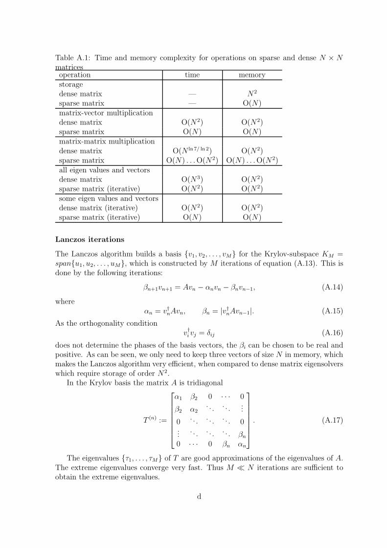
Table A.1: Time and memory complexity for operations on sparse and dense N × Nmatricesoperation time memorystoragedense matrix — N2
sparse matrix — O(N)matrix-vector multiplicationdense matrix O(N2) O(N2)sparse matrix O(N) O(N)matrix-matrix multiplicationdense matrix O(N ln 7/ ln 2) O(N2)sparse matrix O(N) . . .O(N2) O(N) . . .O(N2)all eigen values and vectorsdense matrix O(N3) O(N2)sparse matrix (iterative) O(N2) O(N2)some eigen values and vectorsdense matrix (iterative) O(N2) O(N2)sparse matrix (iterative) O(N) O(N)
Lanczos iterations
The Lanczos algorithm builds a basis {v1, v2, . . . , vM} for the Krylov-subspace KM =span{u1, u2, . . . , uM}, which is constructed by M iterations of equation (A.13). This isdone by the following iterations:
βn+1vn+1 = Avn − αnvn − βnvn−1, (A.14)
whereαn = v†nAvn, βn = |v†nAvn−1|. (A.15)
As the orthogonality conditionv†i vj = δij (A.16)
does not determine the phases of the basis vectors, the βi can be chosen to be real andpositive. As can be seen, we only need to keep three vectors of size N in memory, whichmakes the Lanczos algorithm very efficient, when compared to dense matrix eigensolverswhich require storage of order N2.
In the Krylov basis the matrix A is tridiagonal
T (n) :=
α1 β2 0 · · · 0
β2 α2. . .
. . ....
0. . .
. . .. . . 0
.... . .
. . .. . . βn
0 · · · 0 βn αn
. (A.17)
The eigenvalues {τ1, . . . , τM} of T are good approximations of the eigenvalues of A.The extreme eigenvalues converge very fast. Thus M ≪ N iterations are sufficient toobtain the extreme eigenvalues.
d
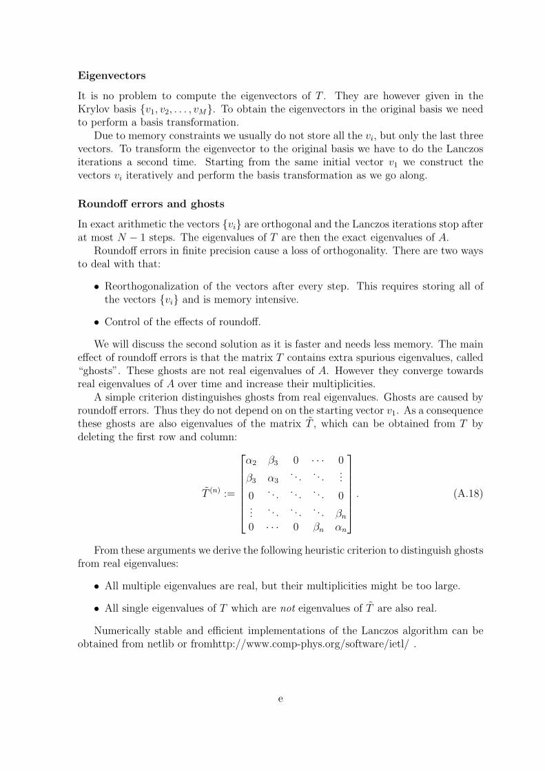
Eigenvectors
It is no problem to compute the eigenvectors of T . They are however given in theKrylov basis {v1, v2, . . . , vM}. To obtain the eigenvectors in the original basis we needto perform a basis transformation.
Due to memory constraints we usually do not store all the vi, but only the last threevectors. To transform the eigenvector to the original basis we have to do the Lanczositerations a second time. Starting from the same initial vector v1 we construct thevectors vi iteratively and perform the basis transformation as we go along.
Roundoff errors and ghosts
In exact arithmetic the vectors {vi} are orthogonal and the Lanczos iterations stop afterat most N − 1 steps. The eigenvalues of T are then the exact eigenvalues of A.
Roundoff errors in finite precision cause a loss of orthogonality. There are two waysto deal with that:
• Reorthogonalization of the vectors after every step. This requires storing all ofthe vectors {vi} and is memory intensive.
• Control of the effects of roundoff.
We will discuss the second solution as it is faster and needs less memory. The maineffect of roundoff errors is that the matrix T contains extra spurious eigenvalues, called“ghosts”. These ghosts are not real eigenvalues of A. However they converge towardsreal eigenvalues of A over time and increase their multiplicities.
A simple criterion distinguishes ghosts from real eigenvalues. Ghosts are caused byroundoff errors. Thus they do not depend on on the starting vector v1. As a consequencethese ghosts are also eigenvalues of the matrix T , which can be obtained from T bydeleting the first row and column:
T (n) :=
α2 β3 0 · · · 0
β3 α3. . .
. . ....
0. . .
. . .. . . 0
.... . .
. . .. . . βn
0 · · · 0 βn αn
. (A.18)
From these arguments we derive the following heuristic criterion to distinguish ghostsfrom real eigenvalues:
• All multiple eigenvalues are real, but their multiplicities might be too large.
• All single eigenvalues of T which are not eigenvalues of T are also real.
Numerically stable and efficient implementations of the Lanczos algorithm can beobtained from netlib or fromhttp://www.comp-phys.org/software/ietl/ .
e