Computational Psycholinguistics Lecture 2: Probabilistic grammars and human sentence

comprehension as incremental probabilistic parsing

Roger Levy University of California – San Diego

ESSLLI 21 July 2009

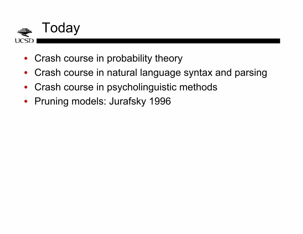
Today

•  Crash course in probability theory

•  Crash course in natural language syntax and parsing

•  Crash course in psycholinguistic methods

•  Pruning models: Jurafsky 1996

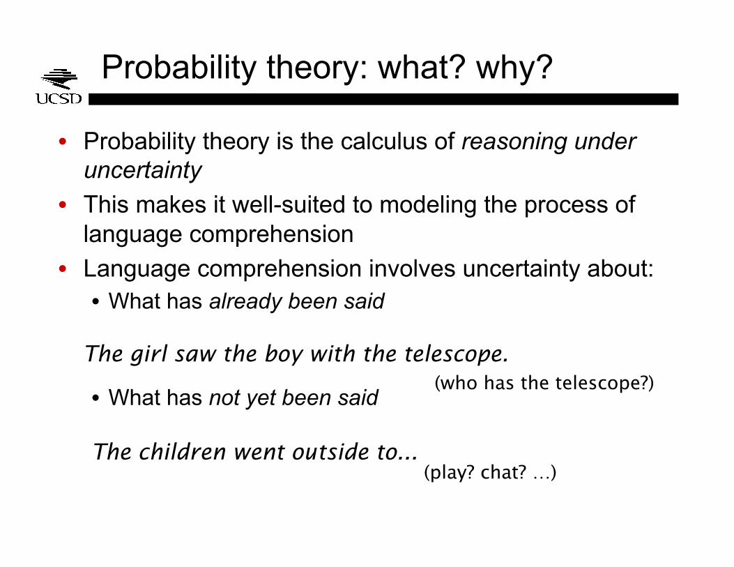
Probability theory: what? why?

•  Probability theory is the calculus of reasoning under uncertainty

•  This makes it well-suited to modeling the process of language comprehension

•  Language comprehension involves uncertainty about: •  What has already been said

•  What has not yet been said

The girl saw the boy with the telescope.

The children went outside to...

(who has the telescope?)

(play? chat? …)

Crash course in probability theory

•  Event space Ω

•  A function P from subsets of Ω to real numbers such that: •  Non-negativity:

•  Properness:

•  Disjoint union:

•  An improper function P for which is called deficient

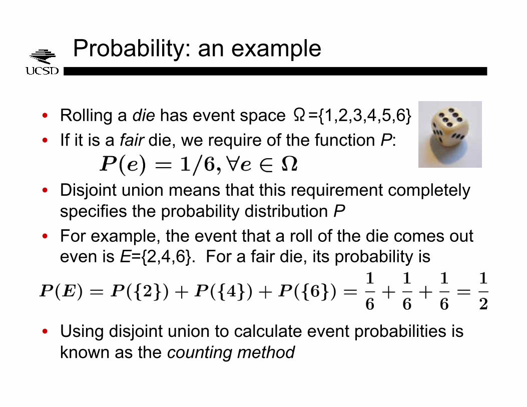
Probability: an example

•  Rolling a die has event space Ω={1,2,3,4,5,6}

•  If it is a fair die, we require of the function P:

•  Disjoint union means that this requirement completely specifies the probability distribution P

•  For example, the event that a roll of the die comes out even is E={2,4,6}. For a fair die, its probability is

•  Using disjoint union to calculate event probabilities is known as the counting method

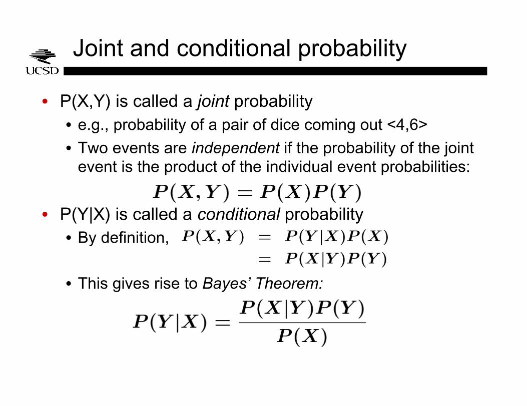
Joint and conditional probability

•  P(X,Y) is called a joint probability •  e.g., probability of a pair of dice coming out <4,6>

•  Two events are independent if the probability of the joint event is the product of the individual event probabilities:

•  P(Y|X) is called a conditional probability •  By definition,

•  This gives rise to Bayes’ Theorem:

Estimating probabilistic models

•  With a fair die, we can calculate event probabilities using the counting method

•  But usually, we can’t deduce the probabilities of the subevents involved

•  Instead, we have to estimate them (=statistics!)

•  Usually, this involves assuming a probabilistic model with some free parameters,* and choosing the values of the free parameters to match empirically obtained data

*(these are parametric estimation methods)

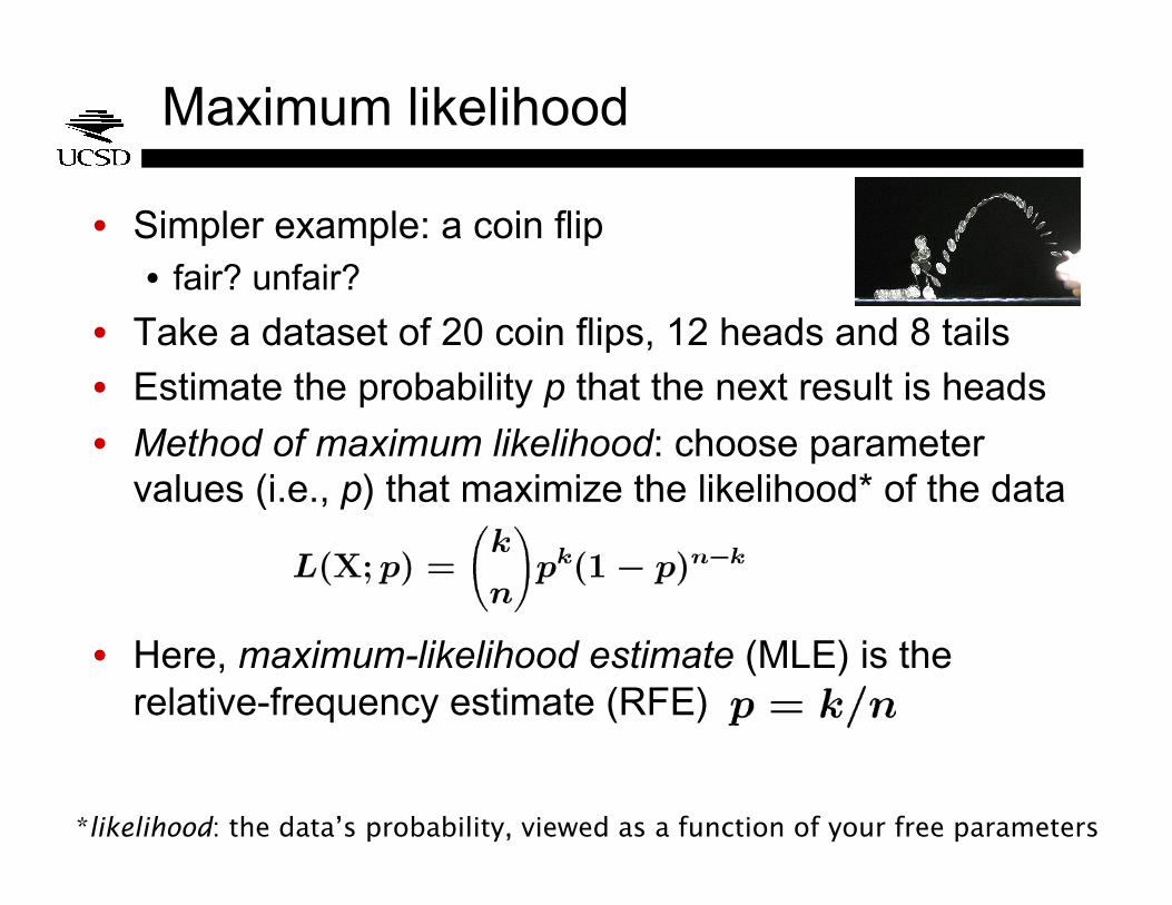
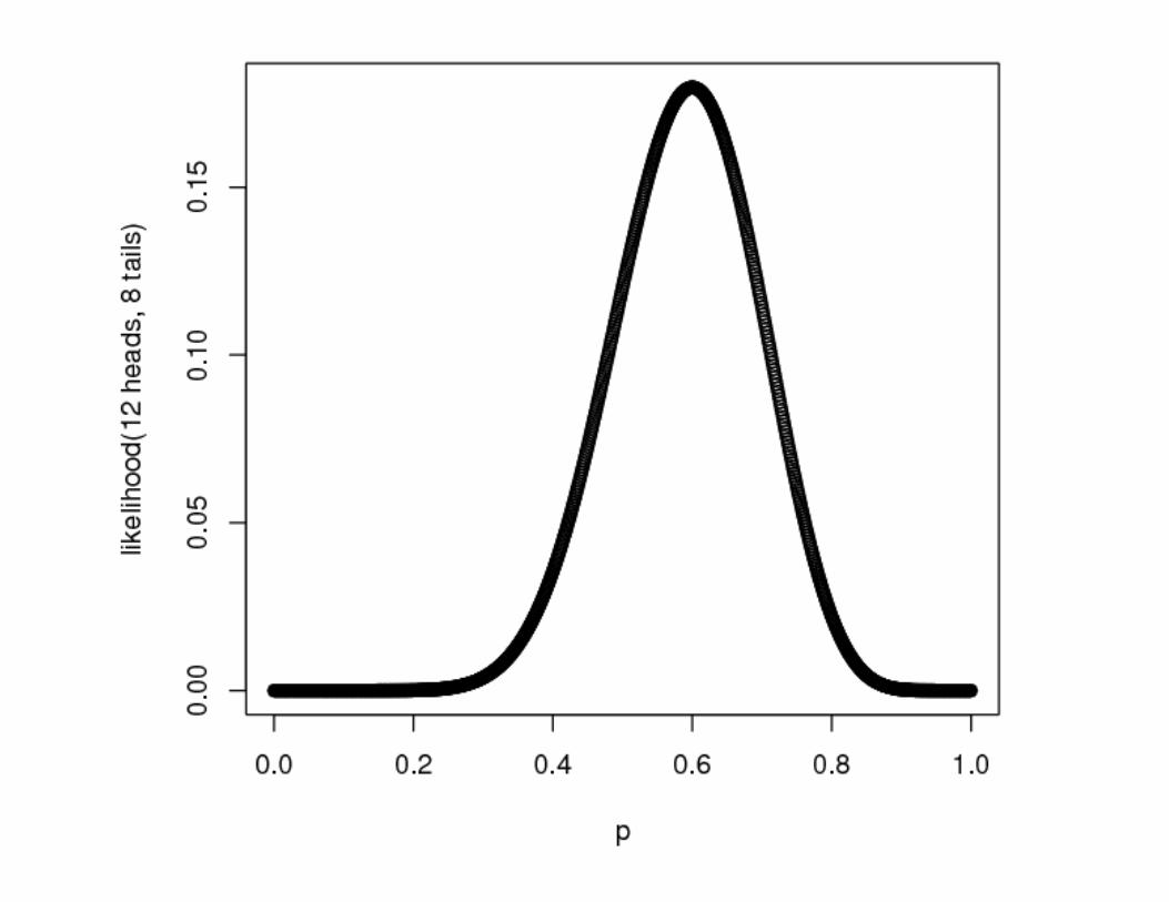
Maximum likelihood

•  Simpler example: a coin flip •  fair? unfair?

•  Take a dataset of 20 coin flips, 12 heads and 8 tails

•  Estimate the probability p that the next result is heads

•  Method of maximum likelihood: choose parameter values (i.e., p) that maximize the likelihood* of the data

•  Here, maximum-likelihood estimate (MLE) is the relative-frequency estimate (RFE)

*likelihood: the data’s probability, viewed as a function of your free parameters

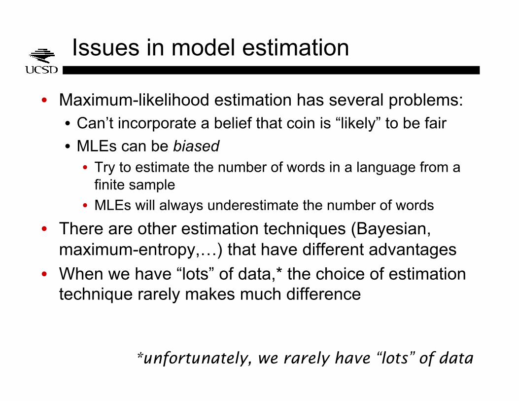
Issues in model estimation

•  Maximum-likelihood estimation has several problems: •  Can’t incorporate a belief that coin is “likely” to be fair

•  MLEs can be biased •  Try to estimate the number of words in a language from a

finite sample

•  MLEs will always underestimate the number of words

•  There are other estimation techniques (Bayesian, maximum-entropy,…) that have different advantages

•  When we have “lots” of data,* the choice of estimation technique rarely makes much difference

*unfortunately, we rarely have “lots” of data

Generative vs. Discriminative Models

•  Inference makes use of conditional probability distr’s

•  Discriminatively-learned models estimate this conditional distribution directly

•  Generatively-learned models estimate the joint probability of data and observation P(O,H) •  Bayes’ theorem is used to find c.p.d. and do inference

probability of … hidden structure … given observations

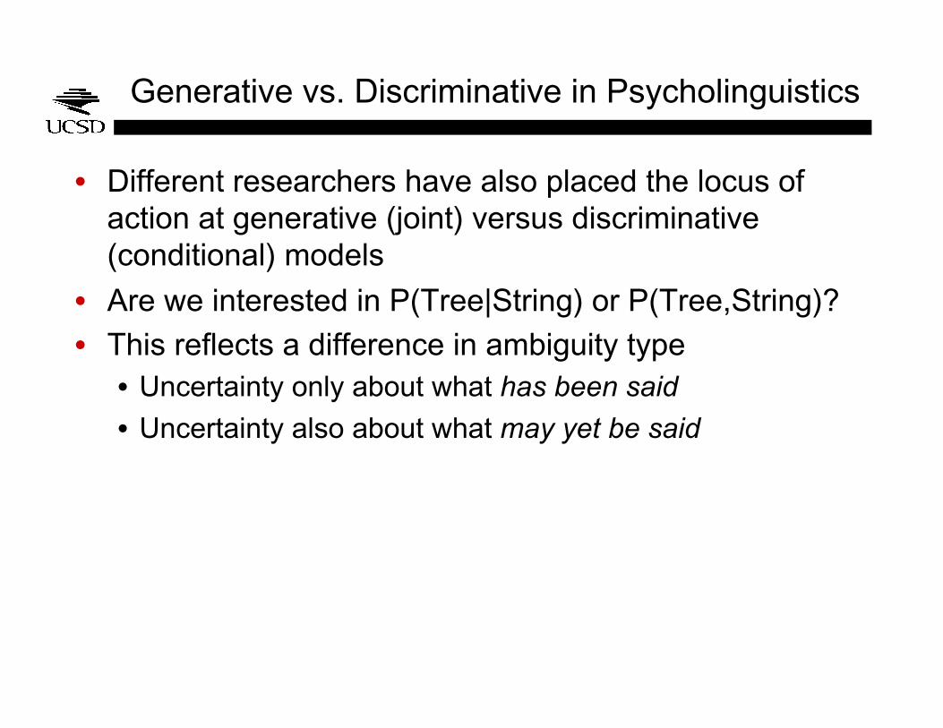
Generative vs. Discriminative in Psycholinguistics

•  Different researchers have also placed the locus of action at generative (joint) versus discriminative (conditional) models

•  Are we interested in P(Tree|String) or P(Tree,String)?

•  This reflects a difference in ambiguity type •  Uncertainty only about what has been said

•  Uncertainty also about what may yet be said

Today

•  Crash course in probability theory

•  Crash course in natural language syntax and parsing

•  Crash course in psycholinguistic methods

•  Pruning models: Jurafsky 1996

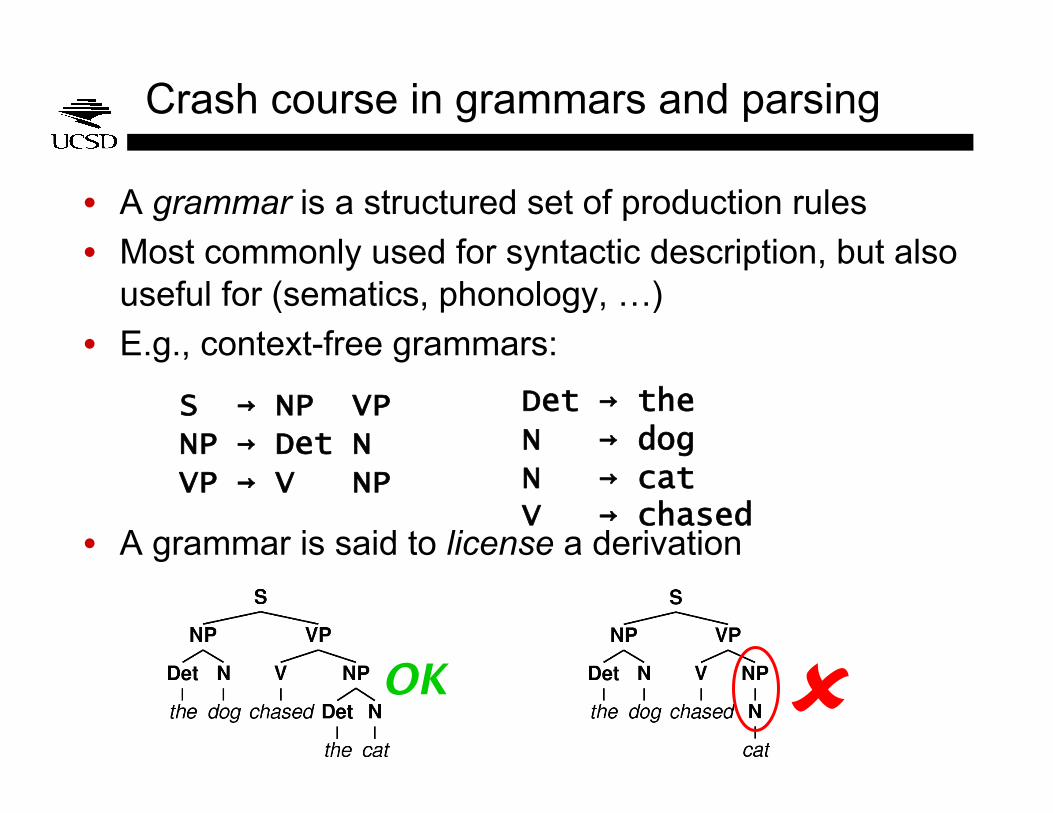
Crash course in grammars and parsing

•  A grammar is a structured set of production rules

•  Most commonly used for syntactic description, but also useful for (sematics, phonology, …)

•  E.g., context-free grammars:

•  A grammar is said to license a derivation

S → NP VP NP → Det N VP → V NP

Det → the N → dog N → cat V → chased

OK

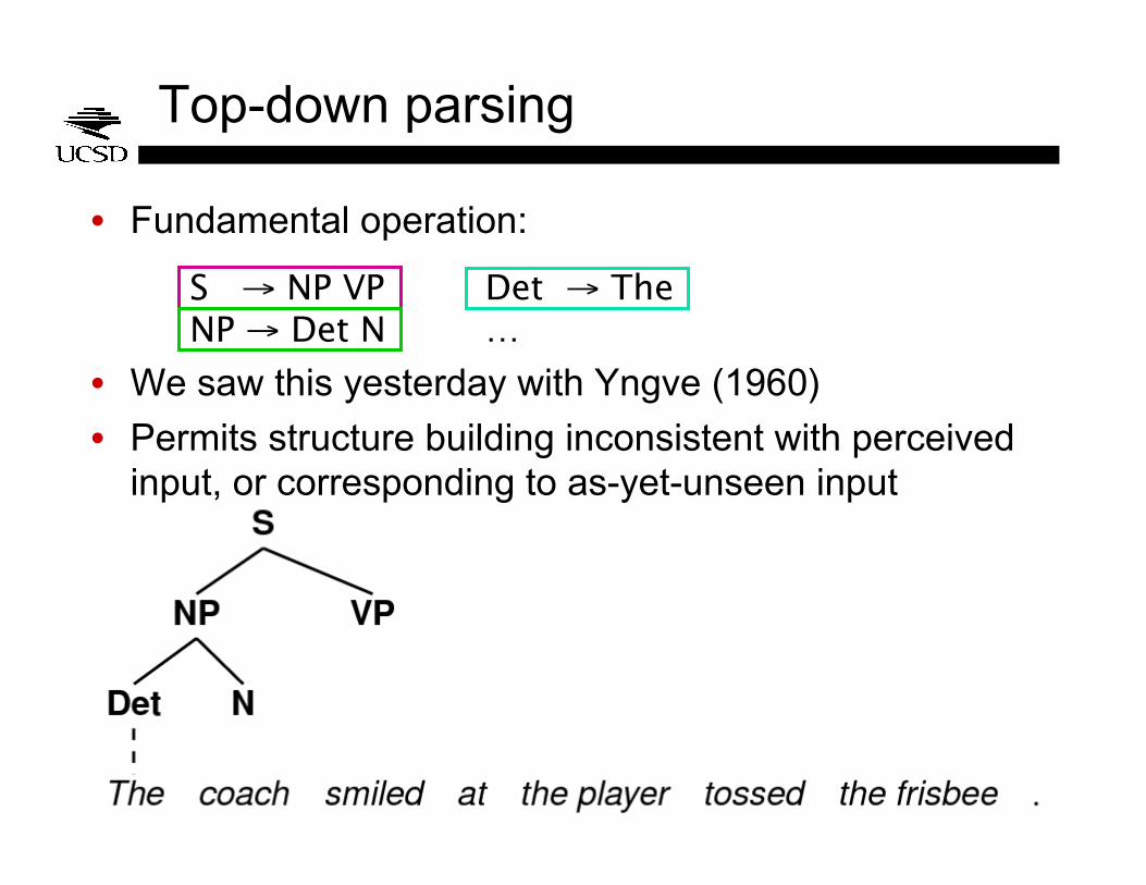
Top-down parsing

•  Fundamental operation:

•  We saw this yesterday with Yngve (1960)

•  Permits structure building inconsistent with perceived input, or corresponding to as-yet-unseen input

S → NP VP NP → Det N

Det → The …

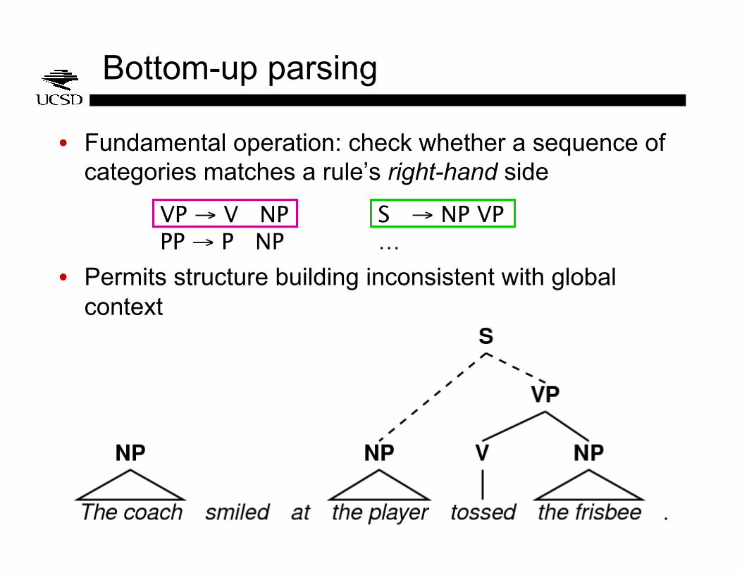
Bottom-up parsing

•  Fundamental operation: check whether a sequence of categories matches a rule’s right-hand side

•  Permits structure building inconsistent with global context

VP → V NP PP → P NP

S → NP VP …

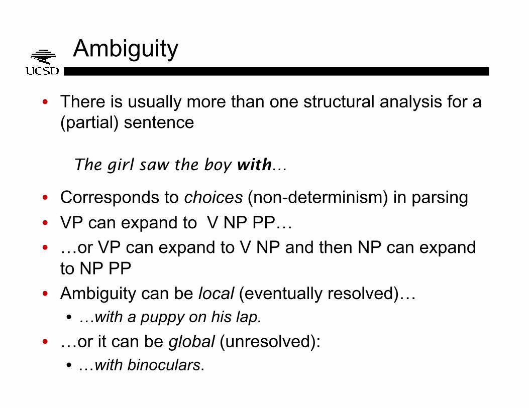
Ambiguity

•  There is usually more than one structural analysis for a (partial) sentence

•  Corresponds to choices (non-determinism) in parsing

•  VP can expand to V NP PP…

•  …or VP can expand to V NP and then NP can expand to NP PP

•  Ambiguity can be local (eventually resolved)… •  …with a puppy on his lap.

•  …or it can be global (unresolved): •  …with binoculars.

The girl saw the boy with…

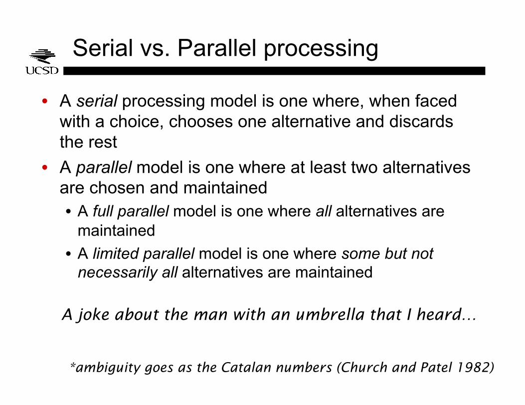
Serial vs. Parallel processing

•  A serial processing model is one where, when faced with a choice, chooses one alternative and discards the rest

•  A parallel model is one where at least two alternatives are chosen and maintained •  A full parallel model is one where all alternatives are

maintained

•  A limited parallel model is one where some but not necessarily all alternatives are maintained

A joke about the man with an umbrella that I heard…

*ambiguity goes as the Catalan numbers (Church and Patel 1982)

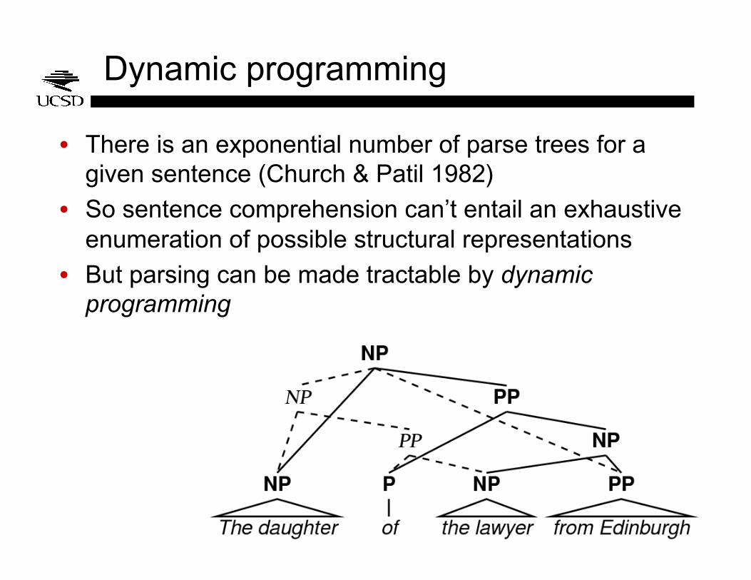
Dynamic programming

•  There is an exponential number of parse trees for a given sentence (Church & Patil 1982)

•  So sentence comprehension can’t entail an exhaustive enumeration of possible structural representations

•  But parsing can be made tractable by dynamic programming

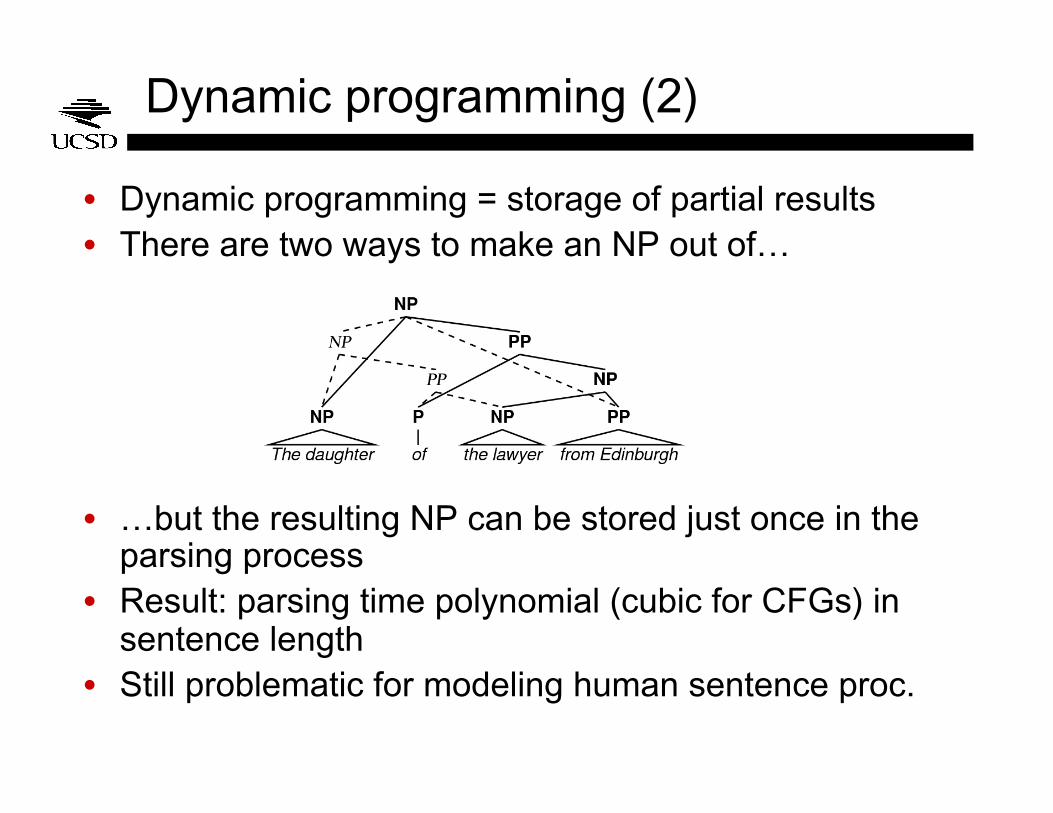
Dynamic programming (2)

•  Dynamic programming = storage of partial results •  There are two ways to make an NP out of…

•  …but the resulting NP can be stored just once in the parsing process

•  Result: parsing time polynomial (cubic for CFGs) in sentence length

•  Still problematic for modeling human sentence proc.

Hybrid bottom-up and top-down

•  Many methods used in practice are combinations of top-down and bottom-up regimens

•  Left-corner parsing: incremental bottom-up parsing with top-down filtering

•  Earley parsing: strictly incremental top-down parsing with top-down filtering and dynamic programming*

*solves problems of left-recursion that occur in top-down parsing

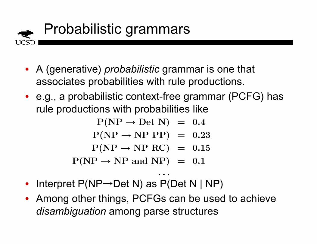
Probabilistic grammars

•  A (generative) probabilistic grammar is one that associates probabilities with rule productions.

•  e.g., a probabilistic context-free grammar (PCFG) has rule productions with probabilities like

•  Interpret P(NP→Det N) as P(Det N | NP)

•  Among other things, PCFGs can be used to achieve disambiguation among parse structures

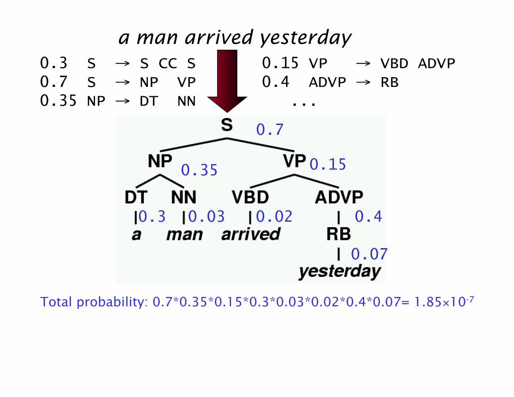
a man arrived yesterday 0.3 S → S CC S 0.15 VP → VBD ADVP 0.7 S → NP VP 0.4 ADVP → RB 0.35 NP → DT NN ...

0.7

0.15 0.35

0.4 0.3 0.03 0.02

0.07

Total probability: 0.7*0.35*0.15*0.3*0.03*0.02*0.4*0.07= 1.85×10-7

Probabilistic grammars (2)

•  A derivation having zero probability corresponds to it being unlicensed in a non-probabilistic setting

•  But “canonical” or “frequent” structures can be distinguished from “marginal” or “rare” structures via the derivation rule probabilities

•  From a computational perspective, this allows probabilistic grammars to increase coverage (number + type of rules) while maintaining ambiguity management

The probabilistic serial↔parallel gradient

•  Suppose two incremental interpretations I1,2 have probabilities p1>0.5>p2 after seeing the last word wi

•  A full-serial model might keep I1 at activation level 1 and discard I2 (i.e., activation level 0)

•  A full-parallel model would keep both I1 and I2 at probabilities p1 and p2 respectively

•  An intermediate model would keep I1 at a1>p1 and I2 at a2<p2

•  (A “hyper-parallel” model might keep I1 at 0.5<a1<p1 and I2 at 0.5>a2>p2)

Today

•  Crash course in probability theory

•  Crash course in natural language syntax and parsing

•  Crash course in psycholinguistic methods

•  Pruning models: Jurafsky 1996

Psycholinguistic methodology

•  The workhorses of psycholinguistic experimentation involve behavioral measures •  What choices do people make in various types of

language-producing and language-comprehending situations?

•  and how long do they take to make these choices?

•  Offline measures •  rating sentences, completing sentences, …

•  Online measures •  tracking people’s eye movements, having people read

words aloud, reading under (implicit) time pressure…

Psycholinguistic methodology (2)

•  [self-paced reading experiment demo now]

Psycholinguistic methodology (3)

•  Caveat: neurolinguistic experimentation more and more widely used to study language comprehension •  methods vary in temporal and spatial resolution

•  people are more passive in these experiments: sit back and listen to/read a sentence, word by word

•  strictly speaking not behavioral measures

•  the question of “what is difficult” becomes a little less straightforward

Today

•  Crash course in probability theory

•  Crash course in natural language syntax and parsing

•  Crash course in psycholinguistic methods

•  Pruning models: Jurafsky 1996

Pruning approaches

•  Jurafsky 1996: a probabilistic approach to lexical access and syntactic disambiguation

•  Main argument: sentence comprehension is probabilistic, construction-based, and parallel

•  Probabilistic parsing model explains •  human disambiguation preferences

•  garden-path sentences

•  The probabilistic parsing model has two components: •  constituent probabilities – a probabilistic CFG model

•  valence probabilities

Jurafsky 1996

•  Every word is immediately completely integrated into the parse of the sentence (i.e., full incrementality)

•  Alternative parses are ranked in a probabilistic model

•  Parsing is limited-parallel: when an alternative parse has unacceptably low probability, it is pruned

•  “Unacceptably low” is determined by beam search (described a few slides later)

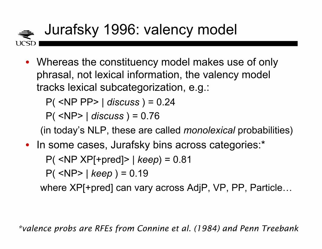
Jurafsky 1996: valency model

•  Whereas the constituency model makes use of only phrasal, not lexical information, the valency model tracks lexical subcategorization, e.g.: P( <NP PP> | discuss ) = 0.24

P( <NP> | discuss ) = 0.76

(in today’s NLP, these are called monolexical probabilities)

•  In some cases, Jurafsky bins across categories:* P( <NP XP[+pred]> | keep) = 0.81

P( <NP> | keep ) = 0.19

where XP[+pred] can vary across AdjP, VP, PP, Particle…

*valence probs are RFEs from Connine et al. (1984) and Penn Treebank

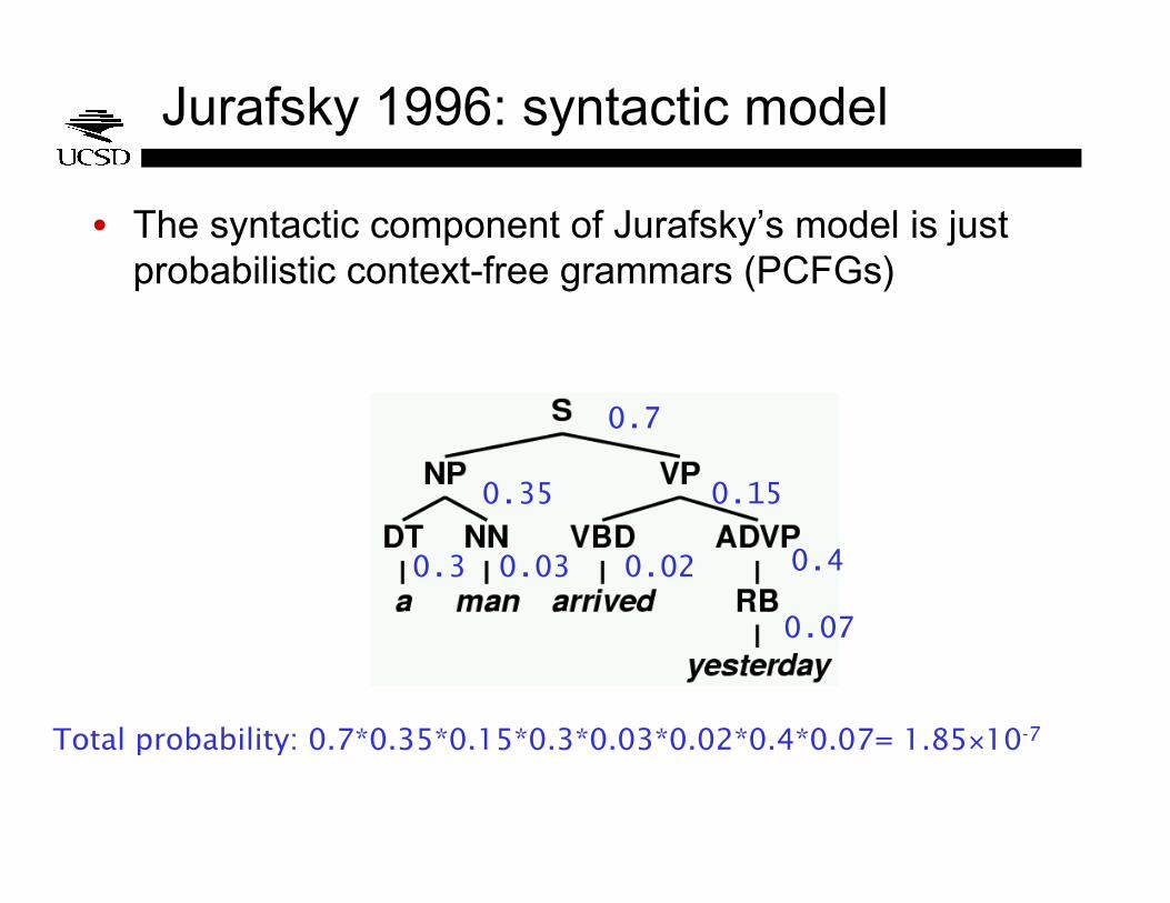
Jurafsky 1996: syntactic model

•  The syntactic component of Jurafsky’s model is just probabilistic context-free grammars (PCFGs)

0.7

0.15 0.35

0.4 0.3 0.03 0.02

0.07

Total probability: 0.7*0.35*0.15*0.3*0.03*0.02*0.4*0.07= 1.85×10-7

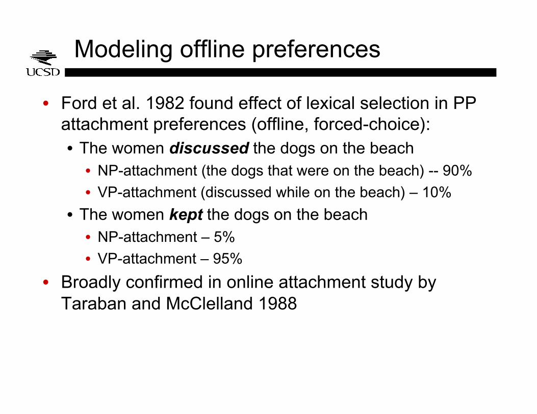
Modeling offline preferences

•  Ford et al. 1982 found effect of lexical selection in PP attachment preferences (offline, forced-choice): •  The women discussed the dogs on the beach •  NP-attachment (the dogs that were on the beach) -- 90%

•  VP-attachment (discussed while on the beach) – 10%

•  The women kept the dogs on the beach •  NP-attachment – 5%

•  VP-attachment – 95%

•  Broadly confirmed in online attachment study by Taraban and McClelland 1988

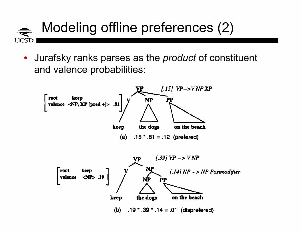
Modeling offline preferences (2)

•  Jurafsky ranks parses as the product of constituent and valence probabilities:

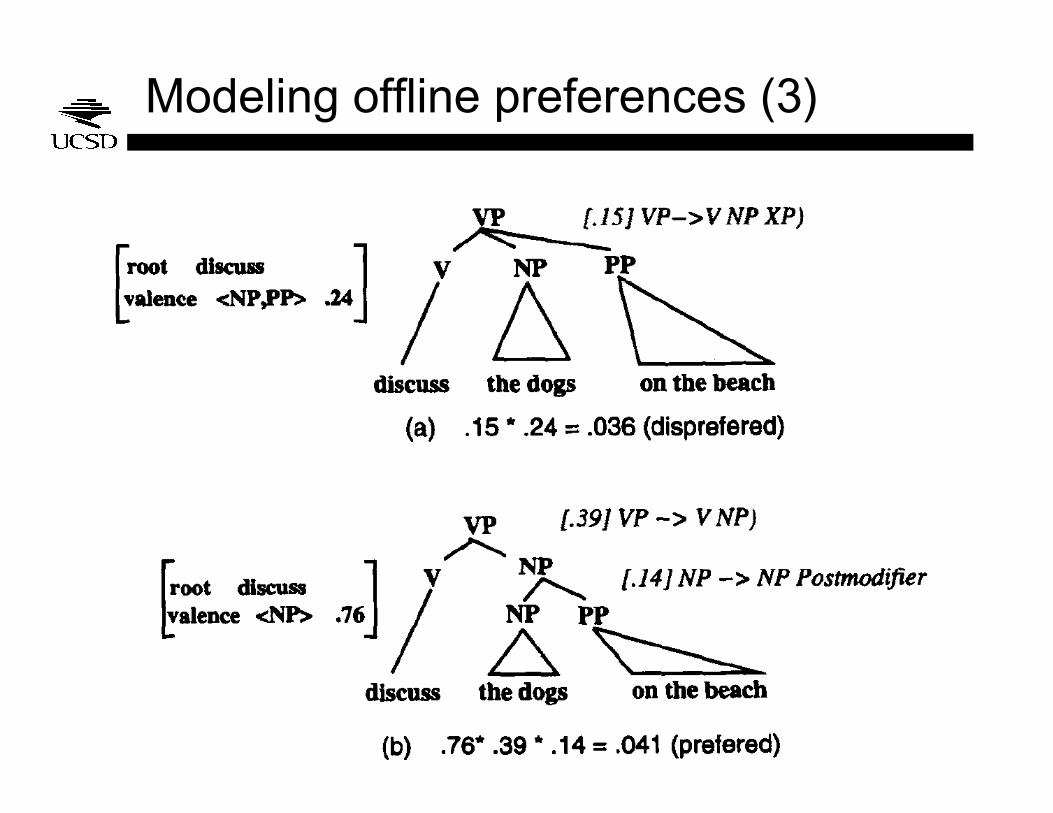
Modeling offline preferences (3)

Result

•  Ranking with respect to parse probability matches offline preferences

•  Note that only monotonicity, not degree of preference is matched

Modeling online parsing

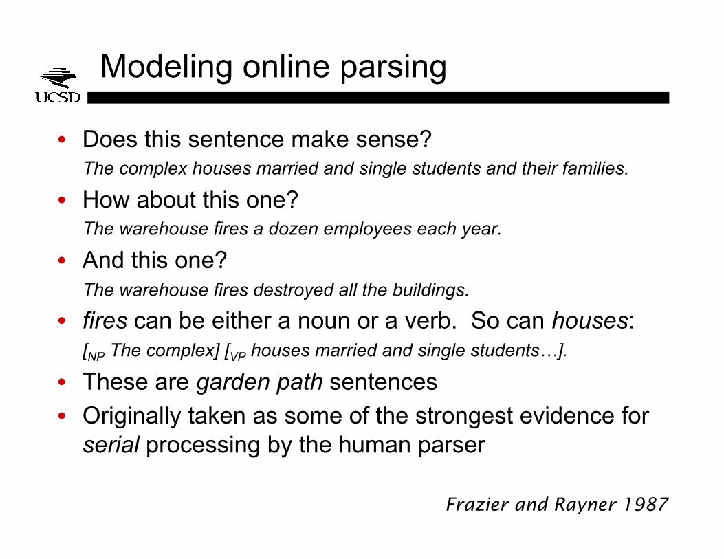
•  Does this sentence make sense? The complex houses married and single students and their families.

•  How about this one? The warehouse fires a dozen employees each year.

•  And this one? The warehouse fires destroyed all the buildings.

•  fires can be either a noun or a verb. So can houses: [NP The complex] [VP houses married and single students…].

•  These are garden path sentences

•  Originally taken as some of the strongest evidence for serial processing by the human parser

Frazier and Rayner 1987

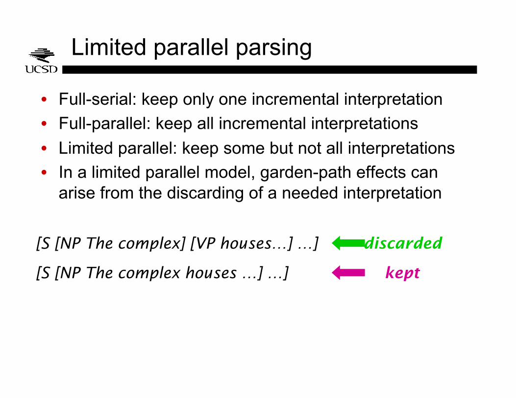
Limited parallel parsing

•  Full-serial: keep only one incremental interpretation

•  Full-parallel: keep all incremental interpretations

•  Limited parallel: keep some but not all interpretations

•  In a limited parallel model, garden-path effects can arise from the discarding of a needed interpretation

[S [NP The complex] [VP houses…] …]

[S [NP The complex houses …] …]

discarded

kept

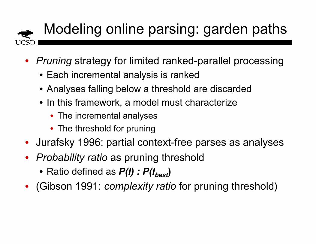
Modeling online parsing: garden paths

•  Pruning strategy for limited ranked-parallel processing •  Each incremental analysis is ranked

•  Analyses falling below a threshold are discarded

•  In this framework, a model must characterize •  The incremental analyses

•  The threshold for pruning

•  Jurafsky 1996: partial context-free parses as analyses

•  Probability ratio as pruning threshold •  Ratio defined as P(I) : P(Ibest)

•  (Gibson 1991: complexity ratio for pruning threshold)

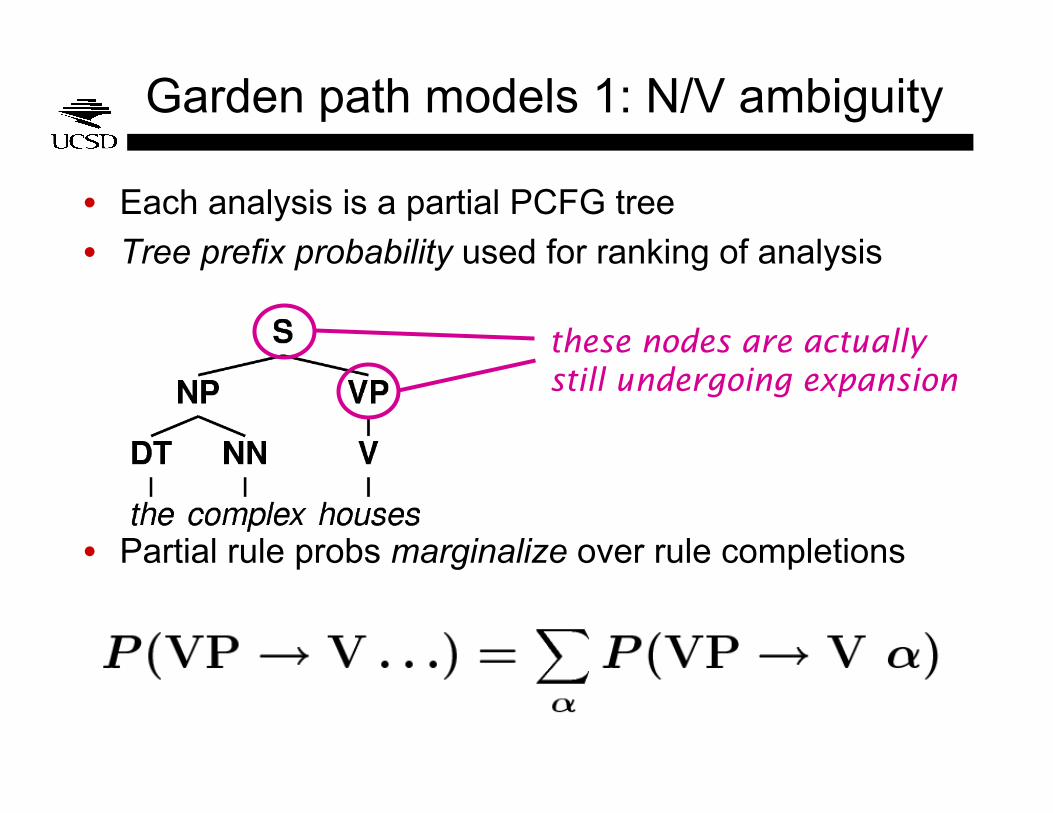
Garden path models 1: N/V ambiguity

•  Each analysis is a partial PCFG tree

•  Tree prefix probability used for ranking of analysis

•  Partial rule probs marginalize over rule completions

these nodes are actually still undergoing expansion

N/V ambiguity (2)

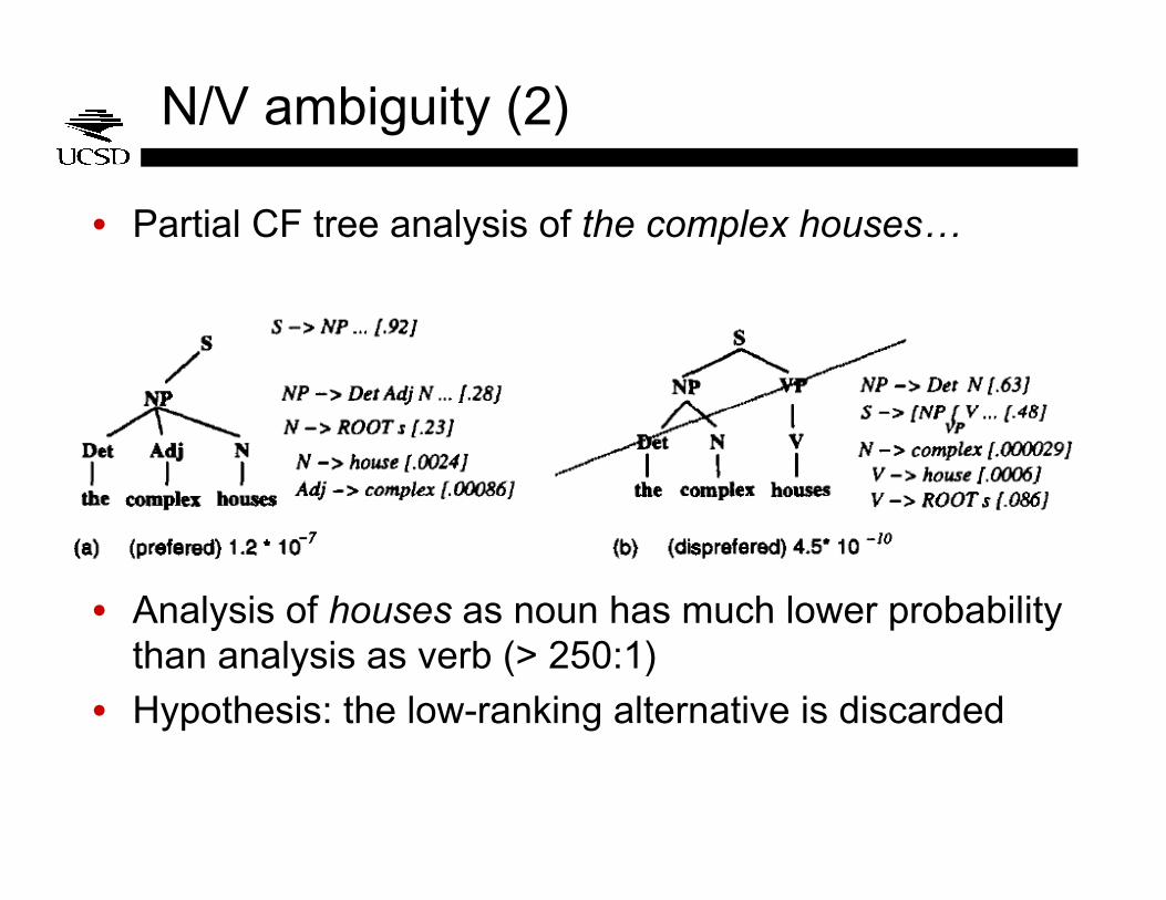
•  Partial CF tree analysis of the complex houses…

•  Analysis of houses as noun has much lower probability than analysis as verb (> 250:1)

•  Hypothesis: the low-ranking alternative is discarded

N/V ambiguity (3)

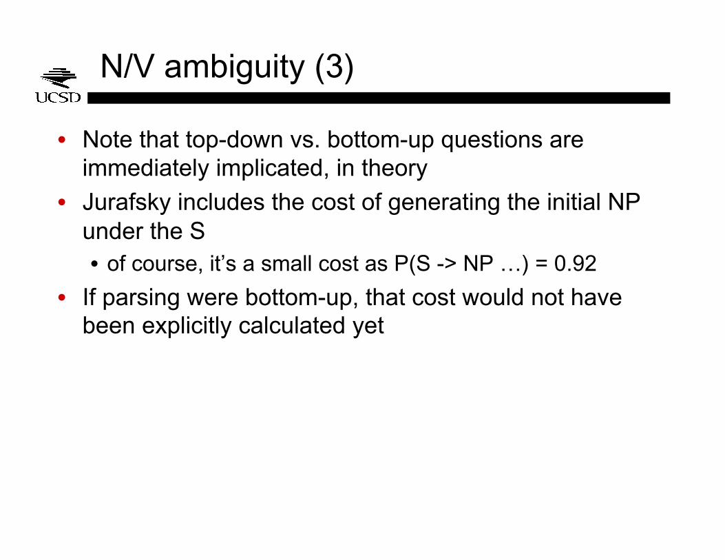
•  Note that top-down vs. bottom-up questions are immediately implicated, in theory

•  Jurafsky includes the cost of generating the initial NP under the S •  of course, it’s a small cost as P(S -> NP …) = 0.92

•  If parsing were bottom-up, that cost would not have been explicitly calculated yet

Garden path models 2

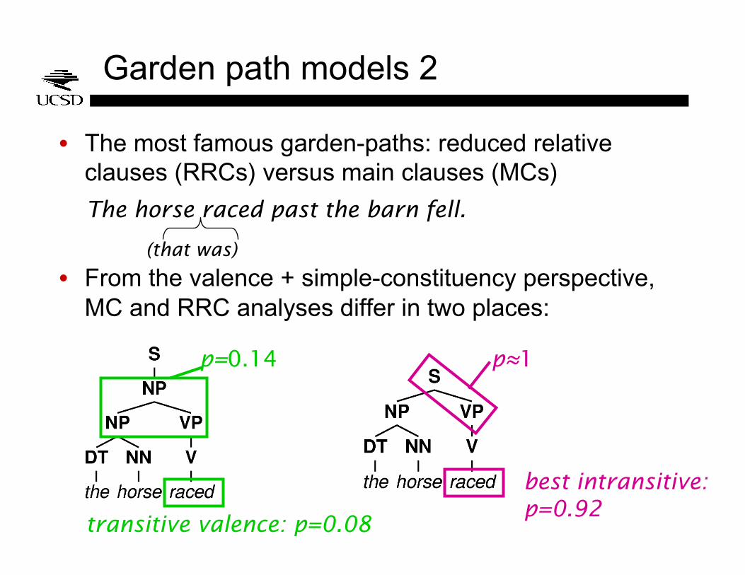
•  The most famous garden-paths: reduced relative clauses (RRCs) versus main clauses (MCs)

•  From the valence + simple-constituency perspective, MC and RRC analyses differ in two places:

The horse raced past the barn fell.

(that was)

p≈1 p=0.14

transitive valence: p=0.08

best intransitive: p=0.92

Garden path models 2, cont.

•  82 : 1 probability ratio means that lower-probability analysis is discarded

•  In contrast, some RRCs do not induce garden paths:

•  Here, the probability ratio turns out to be much closer (≈4 : 1) because found is preferentially transitive

•  Conclusion within pruning theory: beam threshold is between 4 : 1 and 82 : 1

•  (granularity issue: when exactly does probability cost of valence get paid???)

The bird found in the room died.

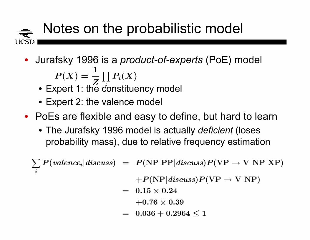
Notes on the probabilistic model

•  Jurafsky 1996 is a product-of-experts (PoE) model

•  Expert 1: the constituency model

•  Expert 2: the valence model

•  PoEs are flexible and easy to define, but hard to learn •  The Jurafsky 1996 model is actually deficient (loses

probability mass), due to relative frequency estimation

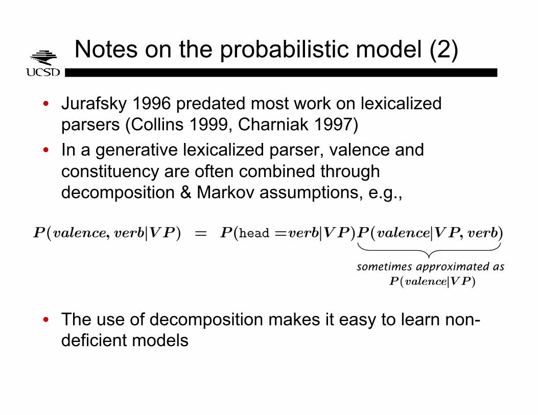
Notes on the probabilistic model (2)

•  Jurafsky 1996 predated most work on lexicalized parsers (Collins 1999, Charniak 1997)

•  In a generative lexicalized parser, valence and constituency are often combined through decomposition & Markov assumptions, e.g.,

•  The use of decomposition makes it easy to learn non-deficient models

sometimes approximated as

Jurafsky 1996 & pruning: main points

•  Syntactic comprehension is probabilistic

•  Offline preferences explained by syntactic + valence probabilities

•  Online garden-path results explained by same model, when beam search/pruning is assumed

General issues

•  What is the granularity of incremental analysis? •  In [NP the complex houses], complex could be an

adjective (=the houses are complex)

•  complex could also be a noun (=the houses of the complex)

•  Should these be distinguished, or combined?

•  When does valence probability cost get paid?

•  What is the criterion for abandoning an analysis?

•  Should the number of maintained analyses affect processing difficulty as well?

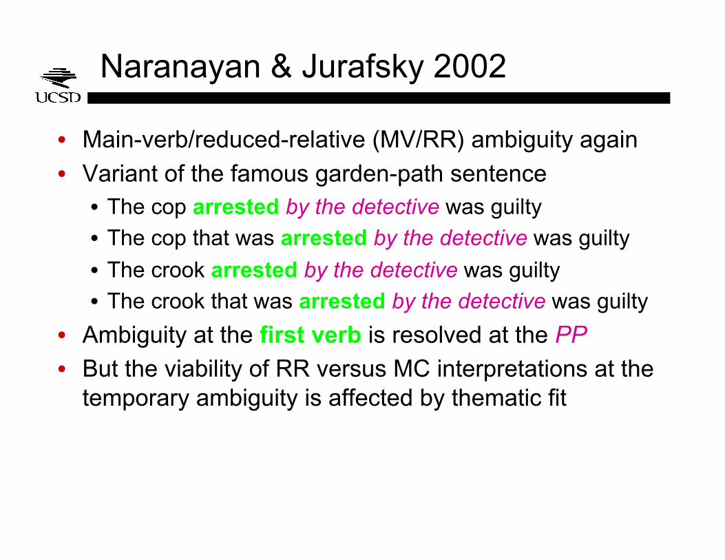
Naranayan & Jurafsky 2002

•  Main-verb/reduced-relative (MV/RR) ambiguity again

•  Variant of the famous garden-path sentence •  The cop arrested by the detective was guilty

•  The cop that was arrested by the detective was guilty

•  The crook arrested by the detective was guilty

•  The crook that was arrested by the detective was guilty

•  Ambiguity at the first verb is resolved at the PP

•  But the viability of RR versus MC interpretations at the temporary ambiguity is affected by thematic fit

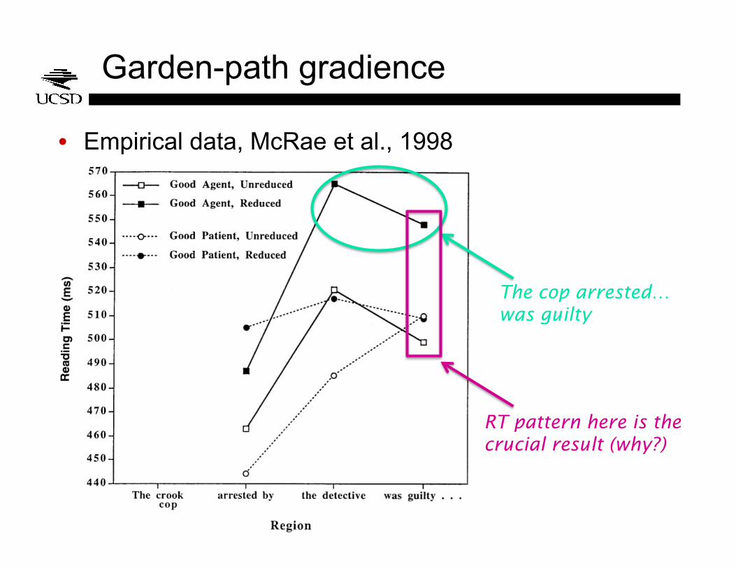
Garden-path gradience

•  Empirical data, McRae et al., 1998

The cop arrested…was guilty

RT pattern here is the crucial result (why?)

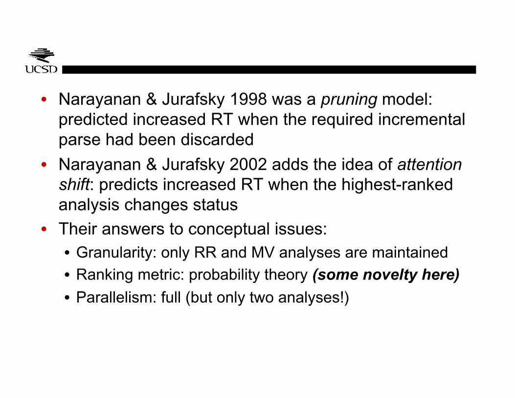
•  Narayanan & Jurafsky 1998 was a pruning model: predicted increased RT when the required incremental parse had been discarded

•  Narayanan & Jurafsky 2002 adds the idea of attention shift: predicts increased RT when the highest-ranked analysis changes status

•  Their answers to conceptual issues: •  Granularity: only RR and MV analyses are maintained

•  Ranking metric: probability theory (some novelty here)

•  Parallelism: full (but only two analyses!)

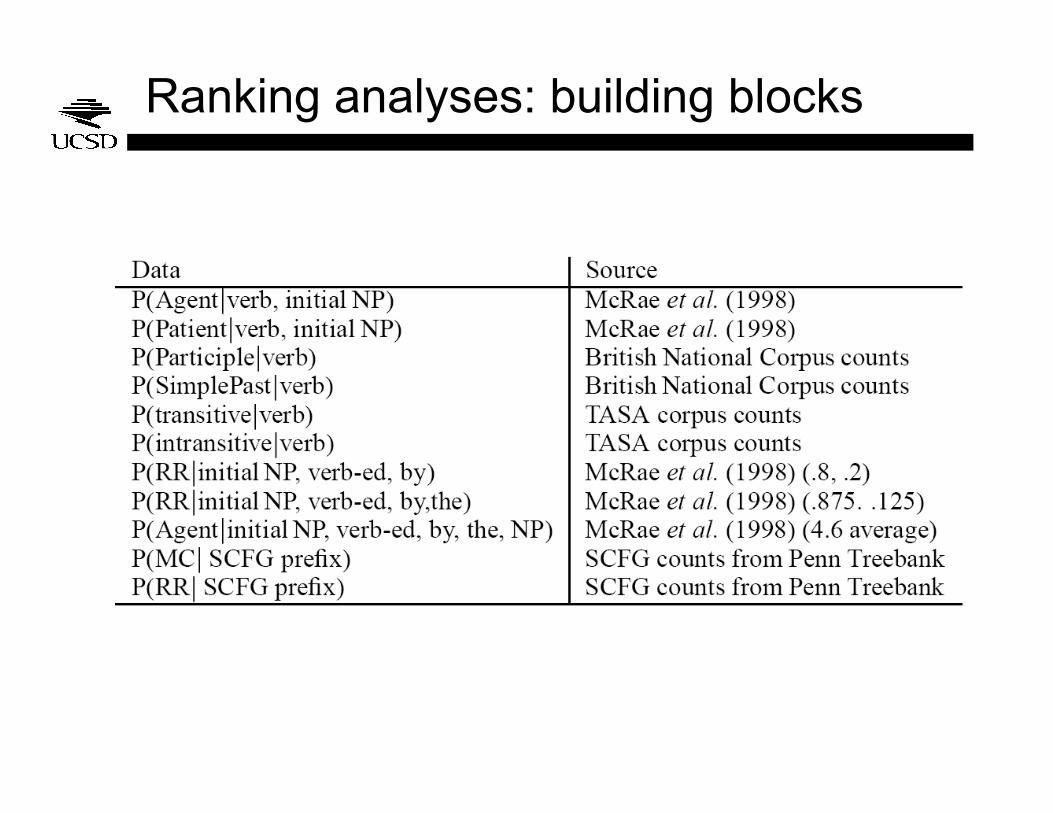
Ranking analyses: building blocks

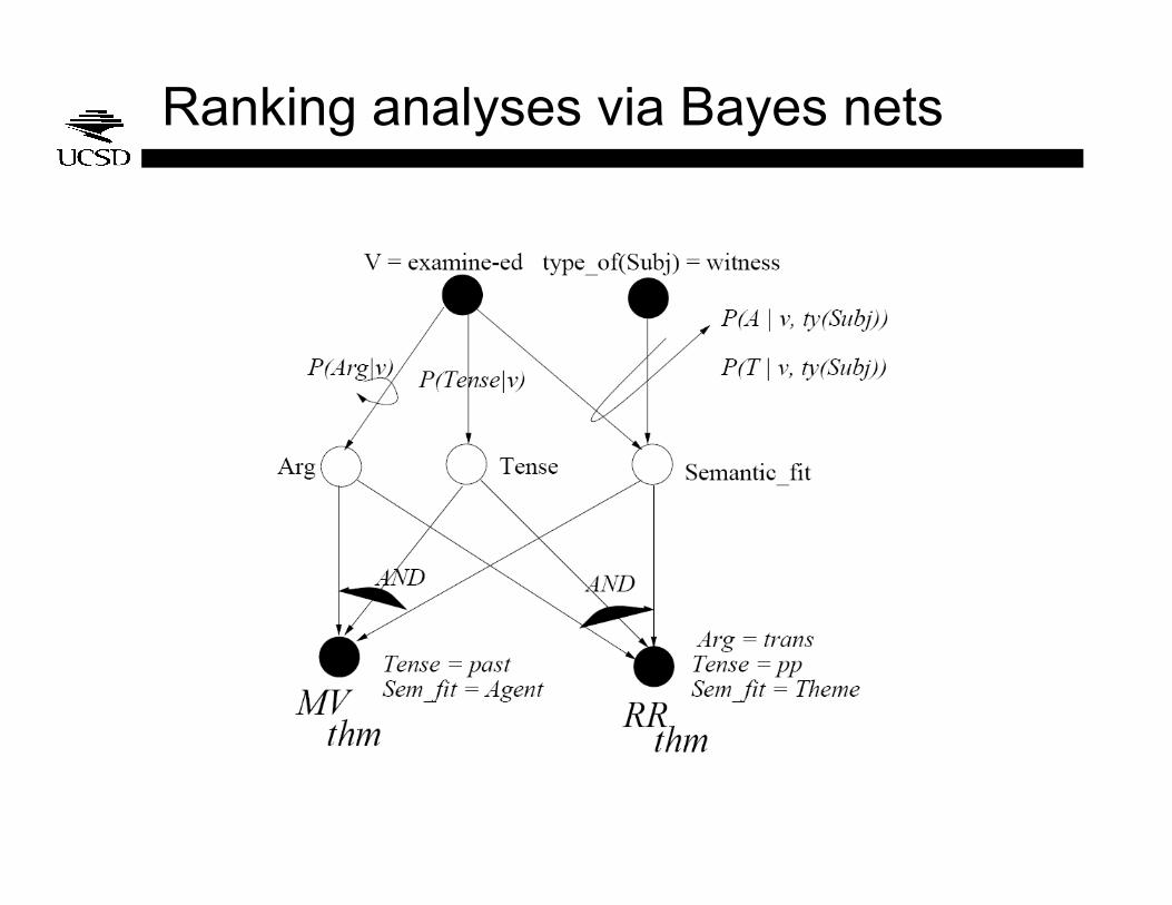
Ranking analyses via Bayes nets

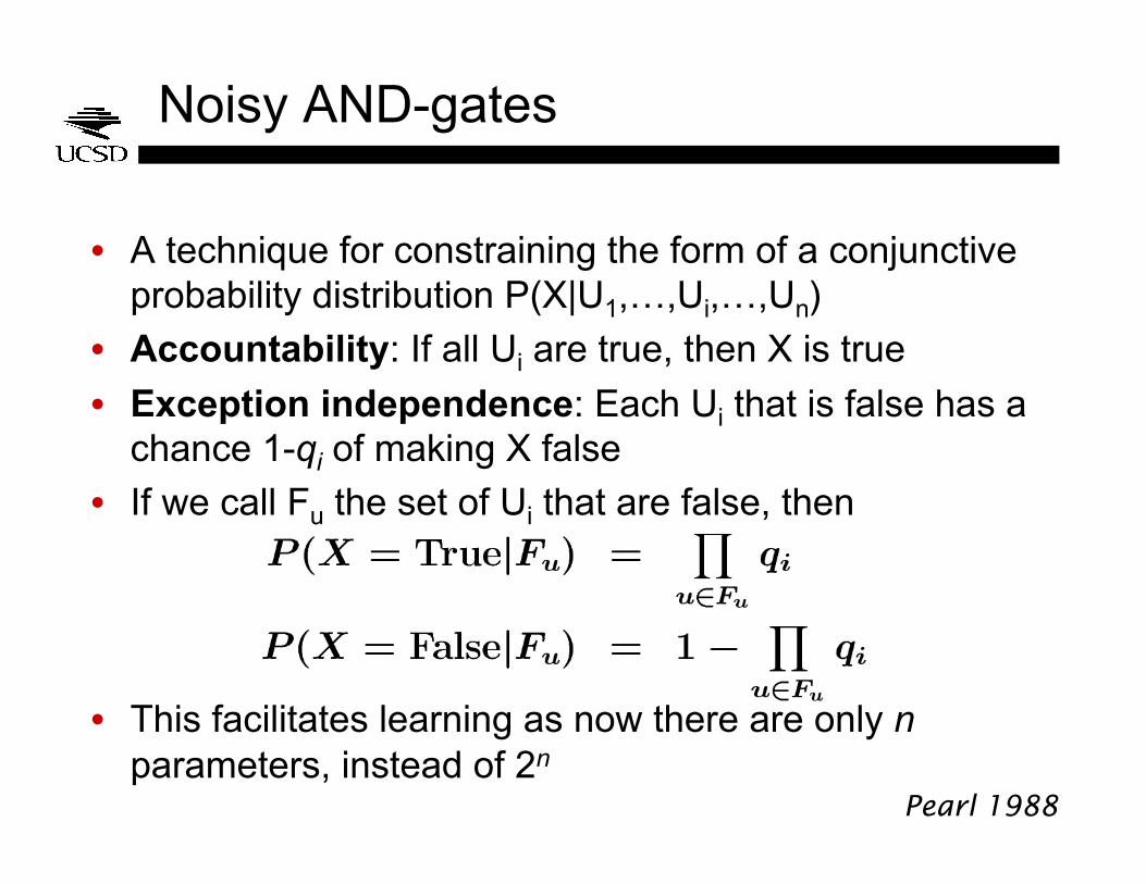
Noisy AND-gates

•  A technique for constraining the form of a conjunctive probability distribution P(X|U1,…,Ui,…,Un)

•  Accountability: If all Ui are true, then X is true

•  Exception independence: Each Ui that is false has a chance 1-qi of making X false

•  If we call Fu the set of Ui that are false, then

•  This facilitates learning as now there are only n parameters, instead of 2n

Pearl 1988

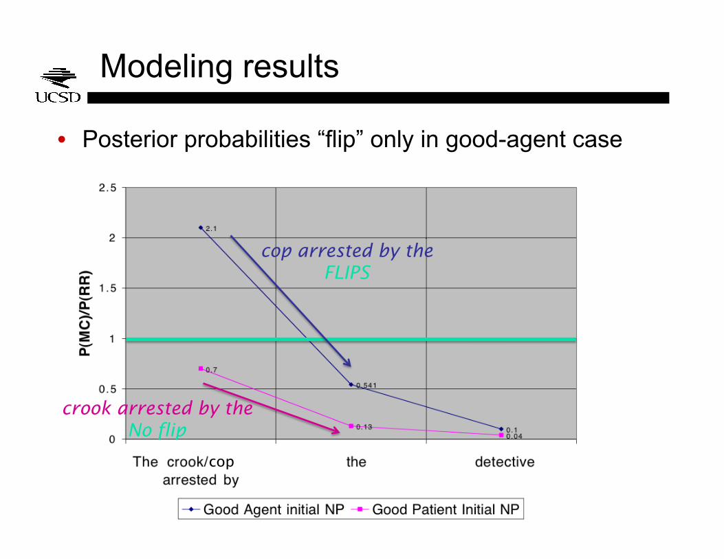
Modeling results

•  Posterior probabilities “flip” only in good-agent case

cop

cop arrested by the FLIPS

crook arrested by the No flip

•  Goes beyond Jurafsky 1996 in two respects •  use of Bayes nets to formalize the probabilistic

relationships between different types of evidence

•  posits attention shift as well as pruning as a source of processing difficulty

For Wednesday

•  Read Hale, 2001; and Levy, Reali, & Griffiths, 2009