Embed Size (px)
Citation preview
ComputationalPhysics Course
17104Lecture 4
Hartmut Ruhl, NilsMoschuring, and
Nina ElkinaLMU,
Theresienstrasse37, Munich, Room
C113
Literature
Spectral analysis
MEs: Intro
MEs: MEs
MEs: Dimless
MEs: Yee
Computational Physics Course 17104Lecture 4
Hartmut Ruhl, Nils Moschuring, and Nina ElkinaLMU, Theresienstrasse 37, Munich, Room C113
Oct 23 - 25, 2012

ComputationalPhysics Course
17104Lecture 4
Hartmut Ruhl, NilsMoschuring, and
Nina ElkinaLMU,
Theresienstrasse37, Munich, Room
C113
Literature
Spectral analysis
MEs: Intro
MEs: MEs
MEs: Dimless
MEs: Yee
Literature
Spectral analysis
MEs: Intro
MEs: MEs
MEs: Dimless
MEs: Yee
ComputationalPhysics Course
17104Lecture 4
Hartmut Ruhl, NilsMoschuring, and
Nina ElkinaLMU,
Theresienstrasse37, Munich, Room
C113
Literature
Spectral analysis
MEs: Intro
MEs: MEs
MEs: Dimless
MEs: Yee
Useful literature
G. Jenkins and D. Watts, Spectral Analysis and ItsApplications, San Francisco: Holden-Day 1968.A. Bondeson, T. Rylander, and P. Ingelstrom,Computational Electromagnetics, Springer, ISBN-10:0-387-26158-3.
ComputationalPhysics Course
17104Lecture 4
Hartmut Ruhl, NilsMoschuring, and
Nina ElkinaLMU,
Theresienstrasse37, Munich, Room
C113
Literature
Spectral analysis
MEs: Intro
MEs: MEs
MEs: Dimless
MEs: Yee
Spectral analysis
The discrete Fourier transform of the vector y is defined as
Yk+1 =
N−1∑j=0
yj+1 e−i 2πjkN , j = 1, ...,N − 1 , (1)
(2)
where the inverse Fourier transform is given by
yj+1 =
N−1∑k=0
Yk+1 e+i 2πjkN . (3)
There is an associated frequency to each point Yk given by
fk =k − 1
τ N, (4)
where τ is the time step size.
ComputationalPhysics Course
17104Lecture 4
Hartmut Ruhl, NilsMoschuring, and
Nina ElkinaLMU,
Theresienstrasse37, Munich, Room
C113
Literature
Spectral analysis
MEs: Intro
MEs: MEs
MEs: Dimless
MEs: Yee
Spectral analysis
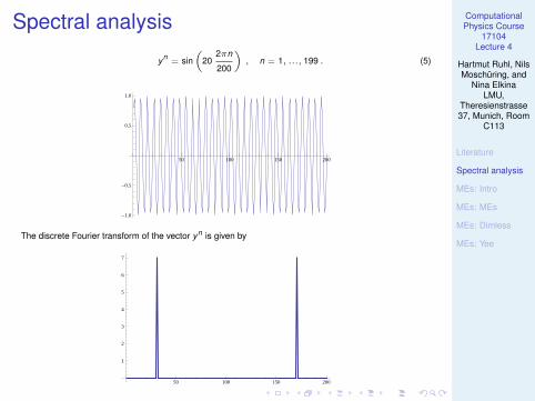
yn = sin(
202πn
200
), n = 1, ..., 199 . (5)
50 100 150 200
-1.0
-0.5
0.5
1.0
The discrete Fourier transform of the vector yn is given by
50 100 150 200
1
2
3
4
5
6
7
ComputationalPhysics Course
17104Lecture 4
Hartmut Ruhl, NilsMoschuring, and
Nina ElkinaLMU,
Theresienstrasse37, Munich, Room
C113
Literature
Spectral analysis
MEs: Intro
MEs: MEs
MEs: Dimless
MEs: Yee
Spectral analysis
Exercise: Write a C-program that generates a discrete data set of the function
y(t) = sin (5 t) + sin (10 t) + sin (20 t)
with adequate resolution. Write a C-program that calculates the discrete Fourier transform of y(t) andplot the real, imaginary, and absolute parts of the discrete Fourier modes either with CAMGRAPH or withPYTHON. Play around with different resolutions.
ComputationalPhysics Course
17104Lecture 4
Hartmut Ruhl, NilsMoschuring, and
Nina ElkinaLMU,
Theresienstrasse37, Munich, Room
C113
Literature
Spectral analysis
MEs: Intro
MEs: MEs
MEs: Dimless
MEs: Yee
Aliasing and Nyquist Frequency
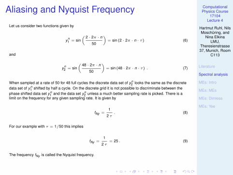
Let us consider two functions given by
yn1 = sin
( 2 · 2π · n
50
)= sin (2 · 2π · n · τ) (6)
and
yn2 = sin
( 48 · 2π · n
50
)= sin (48 · 2π · n · τ) . (7)
When sampled at a rate of 50 for 48 full cycles the discrete data set of yn2 looks the same as the discrete
data set of yn1 shifted by half a cycle. On the discrete grid it is not possible to discriminate between the
phase shifted data set yn1 and the data set yn
2 unless a much better sampling rate is picked. There is alimit on the frequency for any given sampling rate. It is given by
fNy =1
2 τ. (8)
For our example with τ = 1/50 this implies
fNy =1
2 τ= 25 . (9)
The frequency fNy is called the Nyquist frequency.
ComputationalPhysics Course
17104Lecture 4
Hartmut Ruhl, NilsMoschuring, and
Nina ElkinaLMU,
Theresienstrasse37, Munich, Room
C113
Literature
Spectral analysis
MEs: Intro
MEs: MEs
MEs: Dimless
MEs: Yee
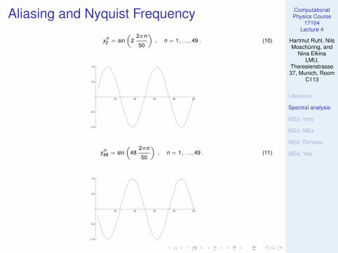
Aliasing and Nyquist Frequency
yn2 = sin
(2
2πn
50
), n = 1, ..., 49 . (10)
10 20 30 40 50
-1.0
-0.5
0.5
1.0
yn48 = sin
(48
2πn
50
), n = 1, ..., 49 . (11)
10 20 30 40 50
-1.0
-0.5
0.5
1.0
ComputationalPhysics Course
17104Lecture 4
Hartmut Ruhl, NilsMoschuring, and
Nina ElkinaLMU,
Theresienstrasse37, Munich, Room
C113
Literature
Spectral analysis
MEs: Intro
MEs: MEs
MEs: Dimless
MEs: Yee
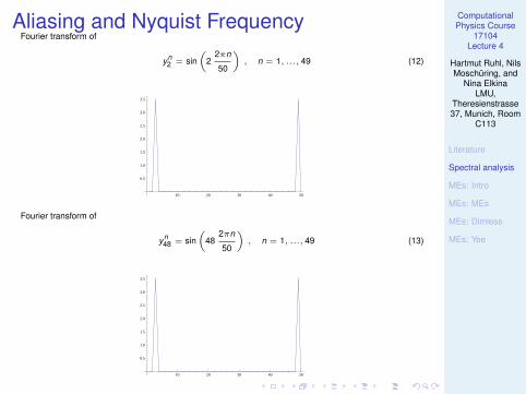
Aliasing and Nyquist FrequencyFourier transform of
yn2 = sin
(2
2πn
50
), n = 1, ..., 49 (12)
10 20 30 40 50
0.5
1.0
1.5
2.0
2.5
3.0
3.5
Fourier transform of
yn48 = sin
(48
2πn
50
), n = 1, ..., 49 (13)
10 20 30 40 50
0.5
1.0
1.5
2.0
2.5
3.0
3.5
ComputationalPhysics Course
17104Lecture 4
Hartmut Ruhl, NilsMoschuring, and
Nina ElkinaLMU,
Theresienstrasse37, Munich, Room
C113
Literature
Spectral analysis
MEs: Intro
MEs: MEs
MEs: Dimless
MEs: Yee
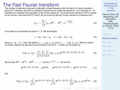
The Fast Fourier transformThe number of operation required to calculate a single frequency with the help of a Fourier transformgoes as N. However, we have to calculate N frequencies to obtain the sprectrum. So it requires N × Noperations to complete the calculation of the Fourier spectrum. The Fast Fourier transform (FFT) is fasteras we will see. How does the FFT work? As we know the discrete Fourier transform is obtained from
Yk+1 =
N−1∑j=0
yj+1 W kj, W kj = e−i 2π jk
N . (14)
Let us take as an example the case N = 8. We decompose
j = 4j2 + 2j1 + j0 , k = 4k2 + 2k1 + k0 , (15)
where j2...k0 = 0, 1 hold. We define yj+1 = y(j2, j1, j0) and Yk+1 = Y (k2, k1, k0). With the help ofour binary notation the discrete Fourier transform for the N = 8 case can be written as
Y (k2, k1, k0) =1∑
j0=0
1∑j1=0
1∑j2=0
y(j2, j1, j0) W (4k2+2k1+k0) (4j2+2j1+j0). (16)
We find that W 8 = W 16 = W 32 = ... = 1 since e−i2πn = 1. So we find
W (4k2+2k1+k0) (4j2) = W 4k0 j2 , W (4k2+2k1+k0) (2j1) = W (2k1+k0) (2j1) (17)
and
Y (k2, k1, k0) =1∑
j0=0
W (4k2+2k1+k0) j01∑
j1=0
W (2k1+k0) (2j1)1∑
j2=0
y(j2, j1, j0) W 4k0 j2 . (18)
ComputationalPhysics Course
17104Lecture 4
Hartmut Ruhl, NilsMoschuring, and
Nina ElkinaLMU,
Theresienstrasse37, Munich, Room
C113
Literature
Spectral analysis
MEs: Intro
MEs: MEs
MEs: Dimless
MEs: Yee
The Fast Fourier transform
The sums can be further simplified by using W 0 = 1. The nested sums are processed as layers. Theinner sum over j2 is evaluated in the first layer as
y1(k0, j1, j0) = y(0, j1, j0) + y(1, j1, j0) W 4k0 (19)
for k0, j1, j0 = 0, 1. The subsequent layers are
y2(k0, k1, j0) = y1(k0, 0, j0) + y1(k0, 1, j0) W (4k1+2k0) (20)
for k0, k1, j0 = 0, 1. The subsequent layers are
y3(k0, k1, k2) = y2(k0, k1, 0) + y2(k0, k1, 1) W (4k2+2k1+k0) (21)
for k0, k1, k1 = 0, 1. Finally, the vector y3 is in bit scrambled form to give Y (k2, k1, k0) = y3(k0, k1, k2).All over only 24 operations were needed.
ComputationalPhysics Course
17104Lecture 4
Hartmut Ruhl, NilsMoschuring, and
Nina ElkinaLMU,
Theresienstrasse37, Munich, Room
C113
Literature
Spectral analysis
MEs: Intro
MEs: MEs
MEs: Dimless
MEs: Yee
Spectral analysis
Exercise: Generate a discrete data set of the function
y(t) = sin (5 t) + sin (10 t) + sin (20 t)
with adequate resolution. Write a C-program that calculates the FFT of y(t) and plot the real, imaginary,and absolute parts of the discrete Fourier modes either with CAMGRAPH or with PYTHON. Play aroundwith different resolutions. Compare the speed of your FFT with your simple-minded version of a Fouriertransform for a selection of sampling rates N. Show that the the FFT scales as N log2 N, while thesimple-minded version scales as N × N.
ComputationalPhysics Course
17104Lecture 4
Hartmut Ruhl, NilsMoschuring, and
Nina ElkinaLMU,
Theresienstrasse37, Munich, Room
C113
Literature
Spectral analysis
MEs: Intro
MEs: MEs
MEs: Dimless
MEs: Yee
Maxwell’s equations: Introduction
The theory of electromagnetism has a wide range of applications.
The Yee algorithm is frequently applied to solve electromegnetic problems.
It is not intended to give a complete account of all appicable numerical methods .
ComputationalPhysics Course
17104Lecture 4
Hartmut Ruhl, NilsMoschuring, and
Nina ElkinaLMU,
Theresienstrasse37, Munich, Room
C113
Literature
Spectral analysis
MEs: Intro
MEs: MEs
MEs: Dimless
MEs: Yee
Maxwell’s equations: Introduction
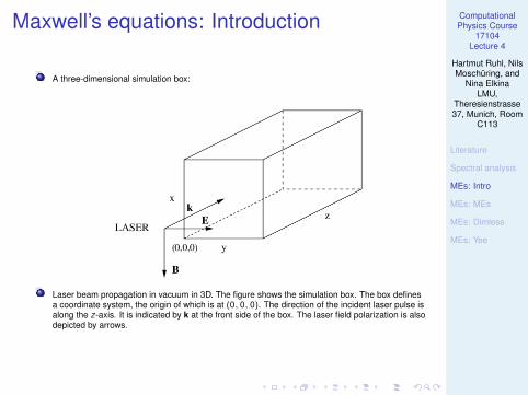
A three-dimensional simulation box:
Laser beam propagation in vacuum in 3D. The figure shows the simulation box. The box definesa coordinate system, the origin of which is at (0, 0, 0). The direction of the incident laser pulse isalong the z-axis. It is indicated by k at the front side of the box. The laser field polarization is alsodepicted by arrows.

ComputationalPhysics Course
17104Lecture 4
Hartmut Ruhl, NilsMoschuring, and
Nina ElkinaLMU,
Theresienstrasse37, Munich, Room
C113
Literature
Spectral analysis
MEs: Intro
MEs: MEs
MEs: Dimless
MEs: Yee
Maxwell’s equations: IntroductionLight diffraction in vacuum:
Laser beam diffraction in vacuum. The setup of the 3D simulation is depicted on the previousslide. The figure shows the 2D contour plot of the field E2
y .
ComputationalPhysics Course
17104Lecture 4
Hartmut Ruhl, NilsMoschuring, and
Nina ElkinaLMU,
Theresienstrasse37, Munich, Room
C113
Literature
Spectral analysis
MEs: Intro
MEs: MEs
MEs: Dimless
MEs: Yee
Maxwell’s equations: Introduction
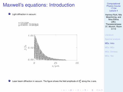
Light diffraction in vacuum:
Laser beam diffraction in vacuum. The figure shows the field amplitude of E2y along the z-axis.
ComputationalPhysics Course
17104Lecture 4
Hartmut Ruhl, NilsMoschuring, and
Nina ElkinaLMU,
Theresienstrasse37, Munich, Room
C113
Literature
Spectral analysis
MEs: Intro
MEs: MEs
MEs: Dimless
MEs: Yee
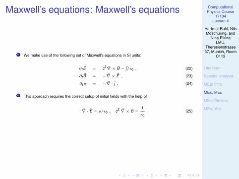
Maxwell’s equations: Maxwell’s equations
We make use of the following set of Maxwell’s equations in SI units:
∂t~E = c2 ~∇× ~B −~j/ε0 , (22)
∂t~B = −~∇× ~E , (23)
∂tρ = −~∇ ·~j . (24)
This approach requires the correct setup of initial fields with the help of
~∇ · ~E = ρ/ε0 , c2 ~∇× B =1
ε0. (25)
ComputationalPhysics Course
17104Lecture 4
Hartmut Ruhl, NilsMoschuring, and
Nina ElkinaLMU,
Theresienstrasse37, Munich, Room
C113
Literature
Spectral analysis
MEs: Intro
MEs: MEs
MEs: Dimless
MEs: Yee
Maxwell’s equations: Dimensionless units
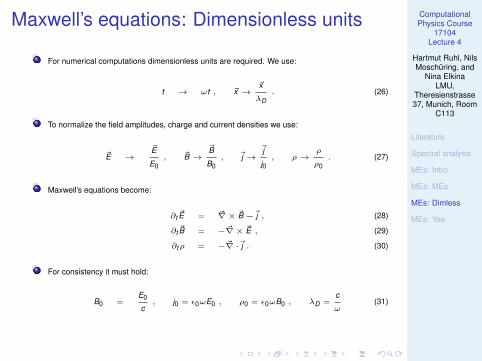
For numerical computations dimensionless units are required. We use:
t → ωt , ~x →~x
λD. (26)
To normalize the field amplitudes, charge and current densities we use:
~E →~E
E0, ~B →
~B
B0, ~j →
~j
j0, ρ→
ρ
ρ0. (27)
Maxwell’s equations become:
∂t~E = ~∇× ~B −~j , (28)
∂t~B = −~∇× ~E , (29)
∂tρ = −~∇ ·~j . (30)
For consistency it must hold:
B0 =E0
c, j0 = ε0ωE0 , ρ0 = ε0ωB0 , λD =
c
ω(31)
ComputationalPhysics Course
17104Lecture 4
Hartmut Ruhl, NilsMoschuring, and
Nina ElkinaLMU,
Theresienstrasse37, Munich, Room
C113
Literature
Spectral analysis
MEs: Intro
MEs: MEs
MEs: Dimless
MEs: Yee
Maxwell’s equations: The Yee algorithm
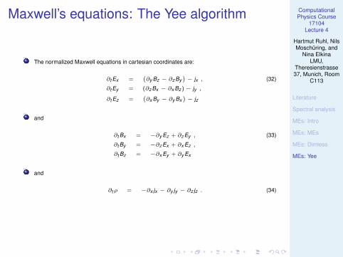
The normalized Maxwell equations in cartesian coordinates are:
∂t Ex =(∂y Bz − ∂z By
)− jx , (32)
∂t Ey = (∂z Bx − ∂x Bz )− jy ,
∂t Ez =(∂x By − ∂y Bx
)− jz
and
∂t Bx = −∂y Ez + ∂z Ey , (33)
∂t By = −∂z Ex + ∂x Ez ,
∂t Bz = −∂x Ey + ∂y Ex
and
∂tρ = −∂x jx − ∂y jy − ∂z jz . (34)
ComputationalPhysics Course
17104Lecture 4
Hartmut Ruhl, NilsMoschuring, and
Nina ElkinaLMU,
Theresienstrasse37, Munich, Room
C113
Literature
Spectral analysis
MEs: Intro
MEs: MEs
MEs: Dimless
MEs: Yee
Maxwell’s equations: The Yee algorithm
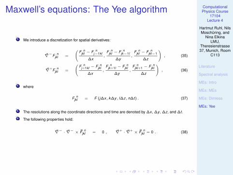
We introduce a discretization for spatial derivatives:
~∇−F njkl =
(F n
jkl − F nj−1kl
∆x,
F njkl − F n
jk−1l
∆y,
F njkl − F n
jkl−1
∆z
), (35)
~∇+F njkl =
(F n
j+1kl − F njkl
∆x,
F njk+1l − F n
jkl
∆y,
F njkl+1 − F n
jkl
∆z
), (36)
where
F njkl = F (j∆x, k∆y, l∆z, n∆t) . (37)
The resolutions along the coordinate directions and time are denoted by ∆x , ∆y , ∆z, and ∆t .
The following properties hold:
~∇− · ~∇− × ~F njkl = 0 , ~∇+ · ~∇+ × ~F n
jkl = 0 . (38)
ComputationalPhysics Course
17104Lecture 4
Hartmut Ruhl, NilsMoschuring, and
Nina ElkinaLMU,
Theresienstrasse37, Munich, Room
C113
Literature
Spectral analysis
MEs: Intro
MEs: MEs
MEs: Dimless
MEs: Yee
Maxwell’s equations: The Yee algorithm
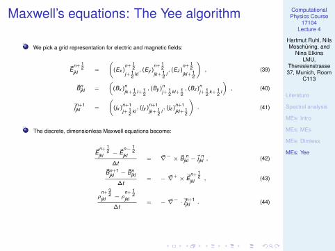
We pick a grid representation for electric and magnetic fields:
~En+ 1
2jkl =
((Ex )
n+ 12
j+ 12 kl, (Ey )
n+ 12
jk+ 12 l, (Ez )
n+ 12
jkl+ 12
), (39)
~Bnjkl =
((Bx )n
jk+ 12 l+ 1
2, (By )n
j+ 12 kl+ 1
2, (Bz )n
j+ 12 k+ 1
2 l
), (40)
~jn+1jkl =
((jx )n+1
j+ 12 kl, (jy )n+1
jk+ 12 l, (jz )n+1
jkl+ 12
). (41)
The discrete, dimensionless Maxwell equations become:
~En+ 1
2jkl − ~E
n− 12
jkl
∆t= ~∇− × ~B n
jkl −~jn
jkl , (42)
~Bn+1jkl −
~Bnjkl
∆t= − ~∇+ × ~E
n+ 12
jkl , (43)
ρn+ 3
2jkl − ρ
n+ 12
jkl
∆t= − ~∇− ·~jn+1
jkl . (44)
ComputationalPhysics Course
17104Lecture 4
Hartmut Ruhl, NilsMoschuring, and
Nina ElkinaLMU,
Theresienstrasse37, Munich, Room
C113
Literature
Spectral analysis
MEs: Intro
MEs: MEs
MEs: Dimless
MEs: Yee
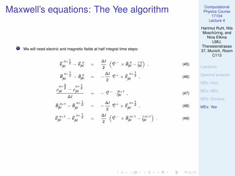
Maxwell’s equations: The Yee algorithm
We will need electric and magnetic fields at half integral time steps:
~En+ 1
2jkl − ~E n
jkl =∆t
2
(~∇− × ~B n
jkl −~jn
jkl
), (45)
~Bn+ 1
2jkl − ~B n
jkl = −∆t
2~∇+ × ~E
n+ 12
jkl , (46)
ρn+ 3
2jkl − ρ
n+ 12
jkl
∆t= − ~∇− ·~jn+1
jkl , (47)
~B n+1jkl − ~B
n+ 12
jkl = −∆t
2~∇+ × ~E
n+ 12
jkl , (48)
~E n+1jkl − ~E
n+ 12
jkl =∆t
2
(~∇− × ~B n+1
jkl −~j n+1jkl
). (49)
ComputationalPhysics Course
17104Lecture 4
Hartmut Ruhl, NilsMoschuring, and
Nina ElkinaLMU,
Theresienstrasse37, Munich, Room
C113
Literature
Spectral analysis
MEs: Intro
MEs: MEs
MEs: Dimless
MEs: Yee
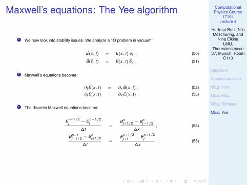
Maxwell’s equations: The Yee algorithm
We now look into stability issues. We analyze a 1D problem in vacuum:
~E(~x, t) = E(x, t)~ez , (50)
~B(~x, t) = B(x, t)~ey . (51)
Maxwell’s equations become:
∂t E(x, t) = ∂x B(x, t) , (52)
∂t B(x, t) = ∂x E(x, t) . (53)
The discrete Maxwell equations become:
En+1/2j − En−1/2
j
∆t=
Bnj+1/2 − Bn
j−1/2
∆x, (54)
Bn+1j+1/2 − Bn
j+1/2
∆t=
En+1/2j+1 − En+1/2
j
∆x. (55)
ComputationalPhysics Course
17104Lecture 4
Hartmut Ruhl, NilsMoschuring, and
Nina ElkinaLMU,
Theresienstrasse37, Munich, Room
C113
Literature
Spectral analysis
MEs: Intro
MEs: MEs
MEs: Dimless
MEs: Yee
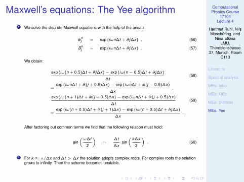
Maxwell’s equations: The Yee algorithm
We solve the discrete Maxwell equations with the help of the ansatz:
Enj = exp (iωn∆t + ikj∆x) , (56)
Bnj = exp (iωn∆t + ikj∆x) . (57)
We obtain:
exp (iω(n + 0.5)∆t + ikj∆x)− exp (iω(n − 0.5)∆t + ikj∆x)
∆t(58)
=exp (iωn∆t + ik(j + 0.5)∆x)− exp (iωn∆t + ik(j − 0.5)∆x)
∆x,
exp (iω(n + 1)∆t + ik(j + 0.5)∆x)− exp (iωn∆t + ik(j + 0.5)∆x)
∆t(59)
=exp (iω(n + 0.5)∆t + ik(j + 1)∆x)− exp (iω(n + 0.5)∆t + ikj∆x)
∆x.
After factoring out common terms we find that the following relation must hold:
sin(ω∆t
2
)=
∆t
∆xsin( k∆x
2
). (60)
For k ≈ π/∆x and ∆t > ∆x the solution adopts complex roots. For complex roots the solutiongrows to infinity. Then the scheme becomes unstable.
ComputationalPhysics Course
17104Lecture 4
Hartmut Ruhl, NilsMoschuring, and
Nina ElkinaLMU,
Theresienstrasse37, Munich, Room
C113
Literature
Spectral analysis
MEs: Intro
MEs: MEs
MEs: Dimless
MEs: Yee
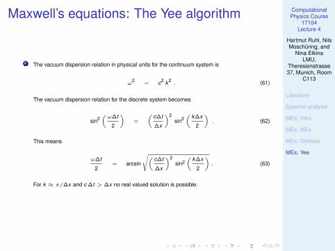
Maxwell’s equations: The Yee algorithm
The vacuum dispersion relation in physical units for the continuum system is
ω2 = c2 k2
. (61)
The vacuum dispersion relation for the discrete system becomes
sin2(ω∆t
2
)=
( c∆t
∆x
)2sin2
( k∆x
2
). (62)
This means
ω∆t
2= arcsin
√( c∆t
∆x
)2sin2
( k∆x
2
). (63)
For k ≈ π/∆x and c ∆t > ∆x no real valued solution is possible.
ComputationalPhysics Course
17104Lecture 4
Hartmut Ruhl, NilsMoschuring, and
Nina ElkinaLMU,
Theresienstrasse37, Munich, Room
C113
Literature
Spectral analysis
MEs: Intro
MEs: MEs
MEs: Dimless
MEs: Yee
Maxwell’s equations: The Yee algorithm
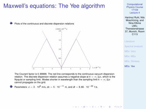
Plots of the continuous and discrete dispersion relations
-3 -2 -1 0 1 2 31. ´ 10-11 k
0.5
1.0
1.5
2.03.3333 ´ 10-20 w
The Courant factor is 0.99999. The red line corresponds to the continuous vacuum dispersionrelation. The discrete dispersion relation assumes a negative slope at k = π/∆x , which is theNyquist or sampling limit. Modes shorter in wavelength than the sampling limit k = π/∆xcannot propagate on the grid.
Parameters: c = 3 · 108 m/s, dx = 5 · 10−11 m, and dt = 6.66 · 10−20 1/s.
ComputationalPhysics Course
17104Lecture 4
Hartmut Ruhl, NilsMoschuring, and
Nina ElkinaLMU,
Theresienstrasse37, Munich, Room
C113
Literature
Spectral analysis
MEs: Intro
MEs: MEs
MEs: Dimless
MEs: Yee
Maxwell’s equations: The Yee algorithm
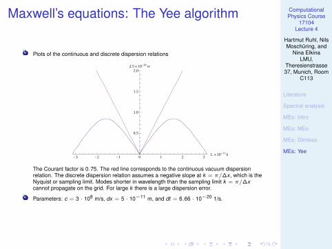
Plots of the continuous and discrete dispersion relations
-3 -2 -1 0 1 2 31. ´ 10-11 k
0.5
1.0
1.5
2.02.5 ´ 10-20 w
The Courant factor is 0.75. The red line corresponds to the continuous vacuum dispersionrelation. The discrete dispersion relation assumes a negative slope at k = π/∆x , which is theNyquist or sampling limit. Modes shorter in wavelength than the sampling limit k = π/∆xcannot propagate on the grid. For large k there is a large dispersion error.
Parameters: c = 3 · 108 m/s, dx = 5 · 10−11 m, and dt = 6.66 · 10−20 1/s.
ComputationalPhysics Course
17104Lecture 4
Hartmut Ruhl, NilsMoschuring, and
Nina ElkinaLMU,
Theresienstrasse37, Munich, Room
C113
Literature
Spectral analysis
MEs: Intro
MEs: MEs
MEs: Dimless
MEs: Yee
Maxwell’s equations: Exercises
Exercise: Analyse the dispersion and stability properties of Maxwell equatons on the FDTD grid in 1Dwith a source current of the form
jz (x, t) = σ Ez (x, t) , (64)
where σ is a constant conductivity. Compare to the dispersion relation in the 1D space-time continuumwith the same current. Which restrictions on resolution do apply for a stable numerical integration of theequations?
Exercise: Write a C-program for a 1D Maxwell solver on the FDTD grid with a source current of the form
jz (x, t) = σ Ez (x, t) , (65)
where σ is a constant conductivity and periodic boundaries. Play with various conductivities andresolutions. Verify your dispersion and stability results empirically.
ComputationalPhysics Course
17104Lecture 4
Hartmut Ruhl, NilsMoschuring, and
Nina ElkinaLMU,
Theresienstrasse37, Munich, Room
C113
Literature
Spectral analysis
MEs: Intro
MEs: MEs
MEs: Dimless
MEs: Yee
Maxwell’s equations: The Yee algorithm
The vacuum dispersion relation in physical units with a finite conductivity σ for the continuumsystem is
ω2 = c2 k2 +
σ2
ε20
, σ =ε0 ω
2p
ω
√1 +
( qE0mcω
)2, ωp =
√√√√ q2n0
ε0m, (66)
where ωp is the plasma frequency. The conductivity assumed here is the one of an ideal plasmawith charge q and density n0. The amplitude of the electric field is E0. The vacuum dispersionrelation for the discrete system becomes
sin2(ω∆t
2
)=
( c ∆t
∆x
)2sin2
( k∆x
2
)+
(∆tσ
2ε0
)2
. (67)
This implies
ω∆t
2= arcsin
√√√√( c∆t
∆x
)2sin2
( k∆x
2
)+
(∆t σ
2ε0
)2
. (68)
For k ≈ π/∆x and c ∆t > ∆x no real valued solution is possible.
ComputationalPhysics Course
17104Lecture 4
Hartmut Ruhl, NilsMoschuring, and
Nina ElkinaLMU,
Theresienstrasse37, Munich, Room
C113
Literature
Spectral analysis
MEs: Intro
MEs: MEs
MEs: Dimless
MEs: Yee
Maxwell’s equations: The Yee algorithm
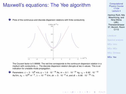
Plots of the continuous and discrete dispersion relations with finite conductivity
-3 -2 -1 0 1 2 31. ´ 10-9 k
0.5
1.0
1.5
2.03.3333 ´ 10-18 w
The Courant factor is 0.99999. The red line corresponds to the continuum dispersion relation in amedium with conductivity σ. The discrete dispersion relation disrupts at two k -values. This is anindication for unstable mode propagation.
Parameters: c = 3 · 108 m/s, q = 1.6 · 10−19 As, m = 9.1 · 10−31 kg, ε0 = 8.82 · 10−12
As/Vm, n0 = 1030 m−3, λ = 10−6 V/m, dx = 5 · 10−9 m, and dt = 6.66 · 10−18 1/s.

ComputationalPhysics Course
17104Lecture 4
Hartmut Ruhl, NilsMoschuring, and
Nina ElkinaLMU,
Theresienstrasse37, Munich, Room
C113
Literature
Spectral analysis
MEs: Intro
MEs: MEs
MEs: Dimless
MEs: Yee
Maxwell’s equations: The Yee algorithm
Plots of the continuous and discrete dispersion relations with finite conductivity
-3 -2 -1 0 1 2 31. ´ 10-11 k
0.5
1.0
1.5
2.03.3333 ´ 10-20 w
The Courant factor is 0.99999. The red line corresponds to the continuum dispersion relation in amedium with conductivity σ. The discrete dispersion relation is well-behaved again. However, thespatial resolution is very high.
Parameters: c = 3 · 108 m/s, q = 1.6 · 10−19 As, m = 9.1 · 10−31 kg, ε0 = 8.82 · 10−12
As/Vm, n0 = 1030 m−3, λ = 10−6 V/m, dx = 5 · 10−11 m, and dt = 6.66 · 10−20 1/s.