Embed Size (px)
Citation preview
Computational Modeling Lab
Wednesday 18 June 2003
Reinforcement Learning an introduction
part 3
Ann Nowé[email protected]://como.vub.ac.be
By Sutton and Barto
Computational Modeling Lab
Policy and Value Iteration
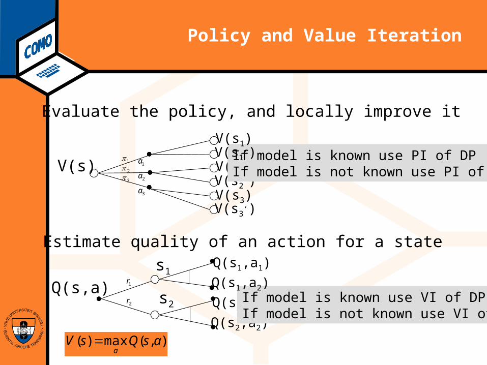
Evaluate the policy, and locally improve it
V(s)V(s2
’)V(s2)
1π2π3π
1a
2a
3a
Q(s,a)
Q(s2,a2)
Q(s2,a1)
1r
2r
s1
s2
Estimate quality of an action for a state
If model is known use PI of DPIf model is not known use PI of RL
If model is known use VI of DPIf model is not known use VI of RL
),(max)( asQsVa
=
Q(s1,a2)
Q(s1,a1)
V(s3’)
V(s3)
V(s1’)
V(s1)
Computational Modeling Lab
Value Functions
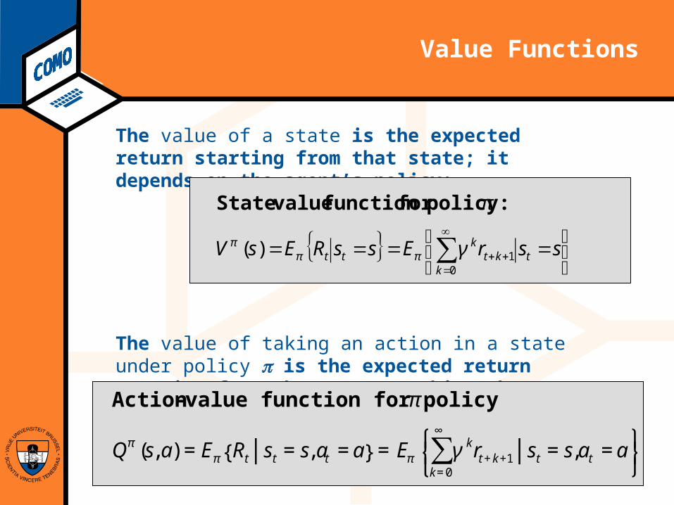
The value of a state is the expected return starting from that state; it depends on the agent’s policy:
The value of taking an action in a state under policy π is the expected return starting from that state, taking that action, and thereafter following π :Action-value function for policy π :
Qπ (s,a) =Eπ Rt st =s,at =a{ }=Eπ γkrt+k+1 st =s,at =ak=0
∞
∑⎧ ⎨ ⎩
⎫ ⎬ ⎭
{ }⎭⎬⎫
⎩⎨⎧
==== ∑∞
=++
01)(
ktkt
ktt ssrEssREsV γ
π
πππ
: policyfor function value-State
Computational Modeling Lab
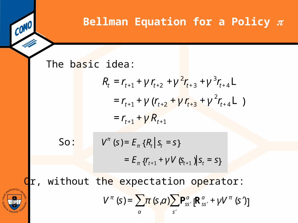
Bellman Equation for a Policy π
Rt =rt+1 +γrt+2 +γ2rt+3 +γ3rt+4L
=rt+1 +γ rt+2 +γrt+3 +γ2rt+4L( )
=rt+1 +γRt+1
The basic idea:
So: Vπ (s)=Eπ Rt st =s{ }
=Eπ rt+1 +γV st+1( ) st =s{ }
Or, without the expectation operator:
€
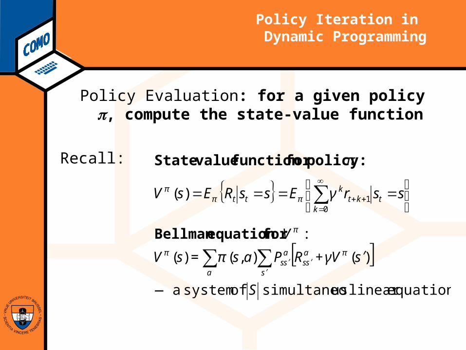
V π (s) = π (s,a) Ps ′ s a Rs ′ s
a + γV π ( ′ s )[ ]′ s
∑a
∑
Computational Modeling Lab
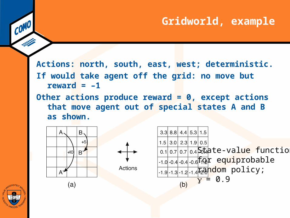
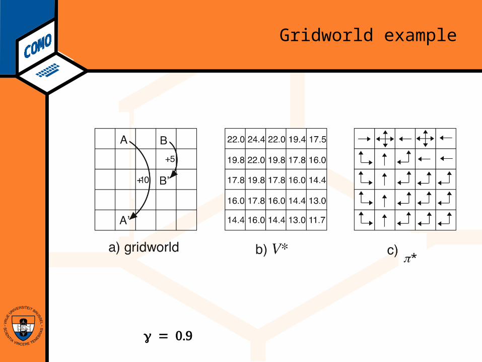
Gridworld, example
Actions: north, south, east, west; deterministic.If would take agent off the grid: no move but reward
= –1Other actions produce reward = 0, except actions
that move agent out of special states A and B as shown.
State-value function for equiprobable random policy; = 0.9
Computational Modeling Lab
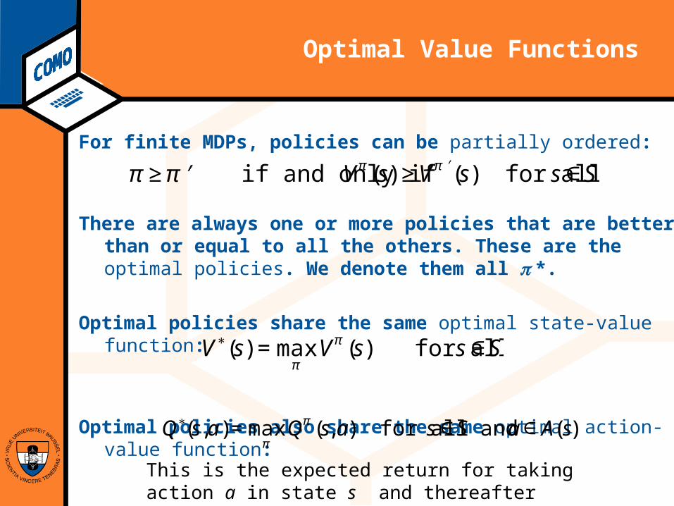
Optimal Value Functions
π ≥ ′ π if and only if Vπ (s) ≥V ′ π (s) for all s∈SFor finite MDPs, policies can be partially ordered:
There are always one or more policies that are better than or equal to all the others. These are the optimal policies. We denote them all π *.
Optimal policies share the same optimal state-value function:
Optimal policies also share the same optimal action-value function:
V∗(s) =maxπ
Vπ (s) for all s∈S
Q∗(s,a)=maxπ
Qπ (s,a) for all s∈S and a∈A(s)
This is the expected return for taking action a in state s and thereafter following an optimal policy.
Computational Modeling Lab
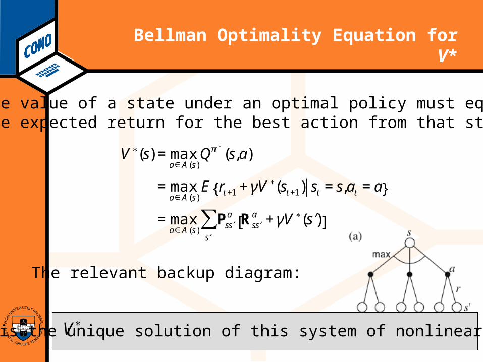
Bellman Optimality Equation for V*
€
V ∗(s) = maxa∈A (s)
Qπ ∗
(s,a)
= maxa∈A (s)
E rt +1 + γV ∗(st +1) st = s,at = a{ }
= maxa∈A (s)
Ps ′ s a
′ s
∑ Rs ′ s a + γV ∗( ′ s )[ ]
The value of a state under an optimal policy must equalthe expected return for the best action from that state:
The relevant backup diagram:
is the unique solution of this system of nonlinear equations.V∗
Computational Modeling Lab
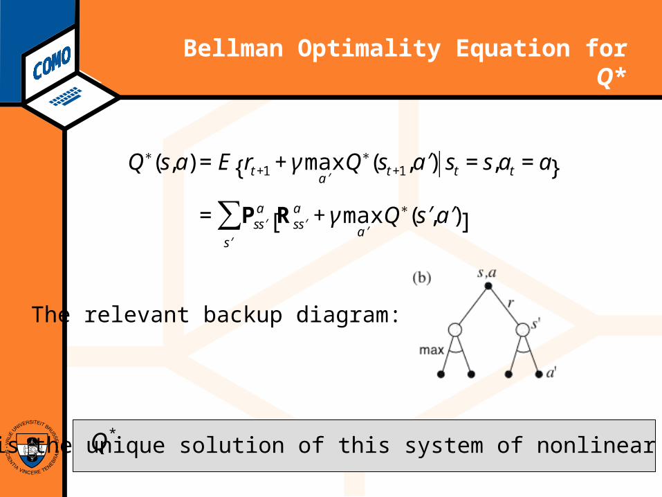
Bellman Optimality Equation for Q*
€
Q∗(s,a) = E rt +1 + γ max′ a
Q∗(st +1, ′ a ) st = s,at = a{ }
= Ps ′ s a Rs ′ s
a + γ max′ a
Q∗( ′ s , ′ a )[ ]′ s
∑
The relevant backup diagram:
is the unique solution of this system of nonlinear equations.Q*
Computational Modeling Lab
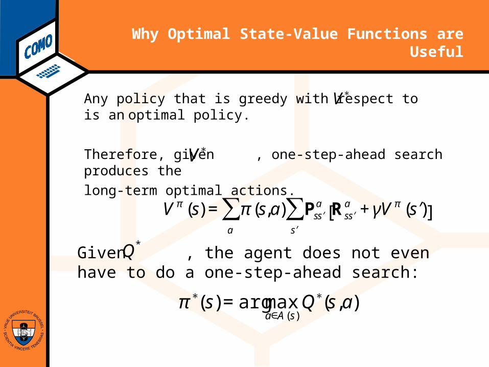
Why Optimal State-Value Functions are Useful
Any policy that is greedy with respect to is an optimal policy.
Therefore, given , one-step-ahead search produces the long-term optimal actions.
€
V π (s) = π (s,a) Ps ′ s a Rs ′ s
a + γV π ( ′ s )[ ]′ s
∑a
∑
V∗
V∗
Given , the agent does not even have to do a one-step-ahead search:
π∗(s)=argmaxa∈A(s)
Q∗(s,a)
Q*
Computational Modeling Lab
Gridworld example
π*
Computational Modeling Lab
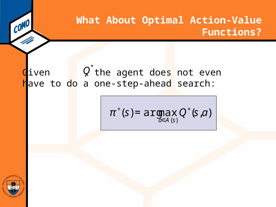
What About Optimal Action-Value Functions?
Given , the agent does not evenhave to do a one-step-ahead search:
Q*
π∗(s)=argmaxa∈A(s)
Q∗(s,a)
Computational Modeling LabPolicy Iteration in Dynamic Programming
Policy Evaluation: for a given policy π, compute the state-value function
{ }⎭⎬⎫
⎩⎨⎧
==== ∑∞
=++
01)(
ktkt
ktt ssrEssREsV γ
π
πππ
: policyfor function value-State
[ ]equations linear ussimultaneo of system a S
sVRPassV
V
a s
ass
ass
—
)(),()(
:
∑ ∑′
′′ ′+= ππ
π
γπ
for equation Bellman
Recall:
Computational Modeling Lab
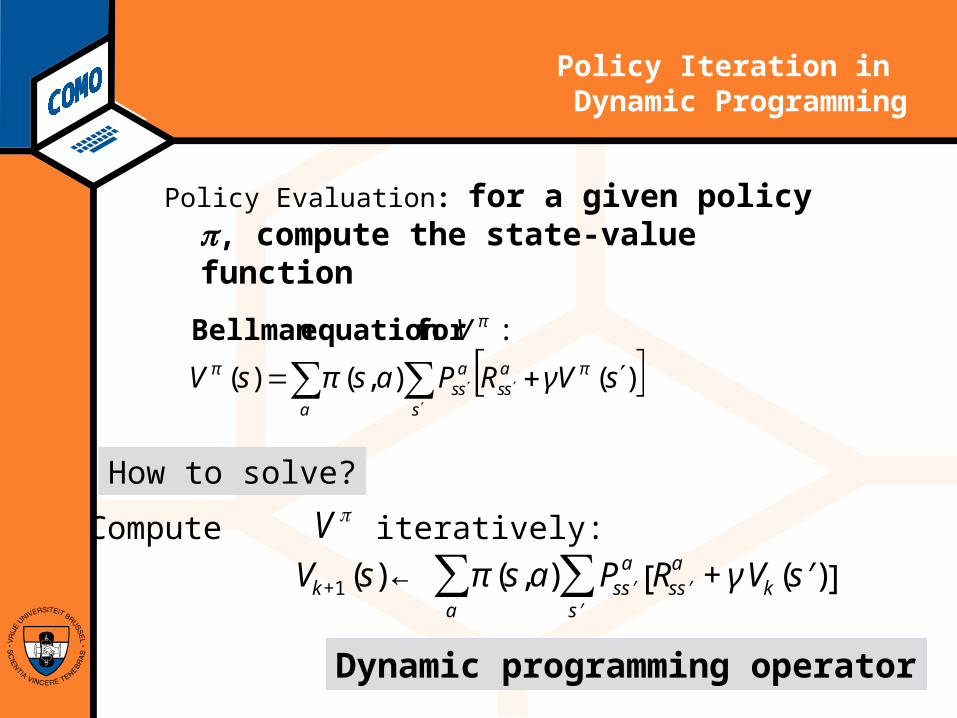
Compute iteratively:
Policy Iteration in Dynamic Programming
Policy Evaluation: for a given policy π, compute the state-value function
[ ]∑ ∑′
′′ ′+=a s
ass
ass sVRPassV
V
)(),()(
:ππ
π
γπ
for equation Bellman
Vk+1(s)← π(s,a) Ps ′ s a Rs ′ s
a +γVk( ′ s )[ ]′ s
∑a∑
πV
How to solve?
Dynamic programming operator
Computational Modeling Lab
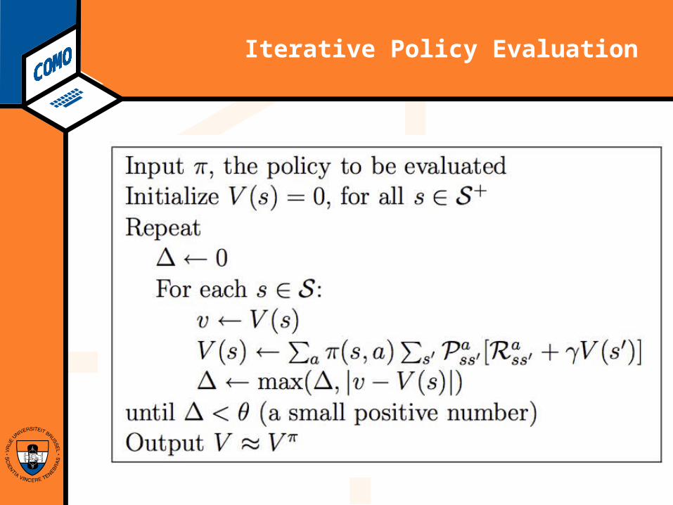
Iterative Policy Evaluation
Computational Modeling Lab
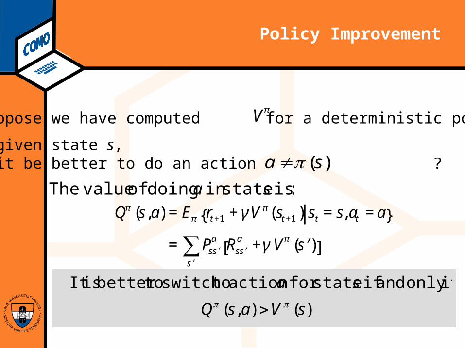
Policy Improvement
Suppose we have computed for a deterministic policy π.Vπ
For a given state s, would it be better to do an action ? )(sa π≠
Qπ (s,a) =Eπ rt+1 +γVπ(st+1) st =s,at =a{ }
= Ps ′ s a
′ s ∑ Rs ′ s
a +γVπ ( ′ s )[ ]
:is state in doing of value The sa
)(),( sVasQ
saππ >
ifonly and if state for action to switch to better is It
Computational Modeling Lab
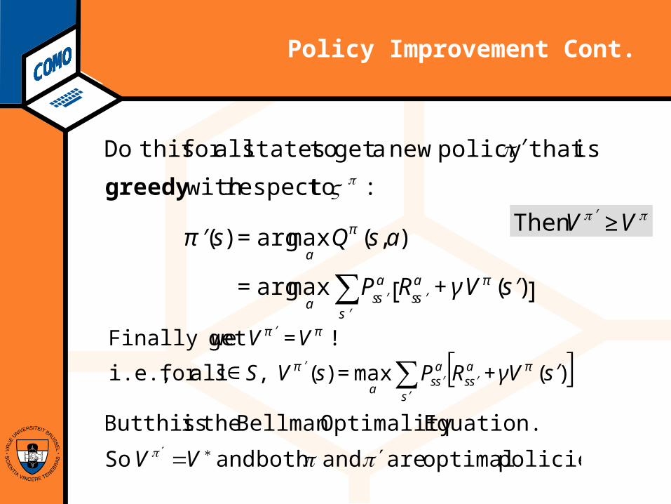
Policy Improvement Cont.
′ π (s) =argmaxa
Qπ (s,a)
=argmaxa
Ps ′ s a
′ s ∑ Rs ′ s
a +γVπ ( ′ s )[ ]
:π
πV to respect with
is that policy new a get to states all for this Do
greedy
′
ππ VV ≥′Then
[ ] , all for i.e.,
! get Finally we
)(max)( sVRPsVSs
VVass
s
ass
a′+=∈
=
′′
′′
′
∑ ππ
ππ
γ
policies. optimal are and both and So
Equation. Optimality Bellman the is this But
πππ ′= ∗′ VV
Computational Modeling Lab
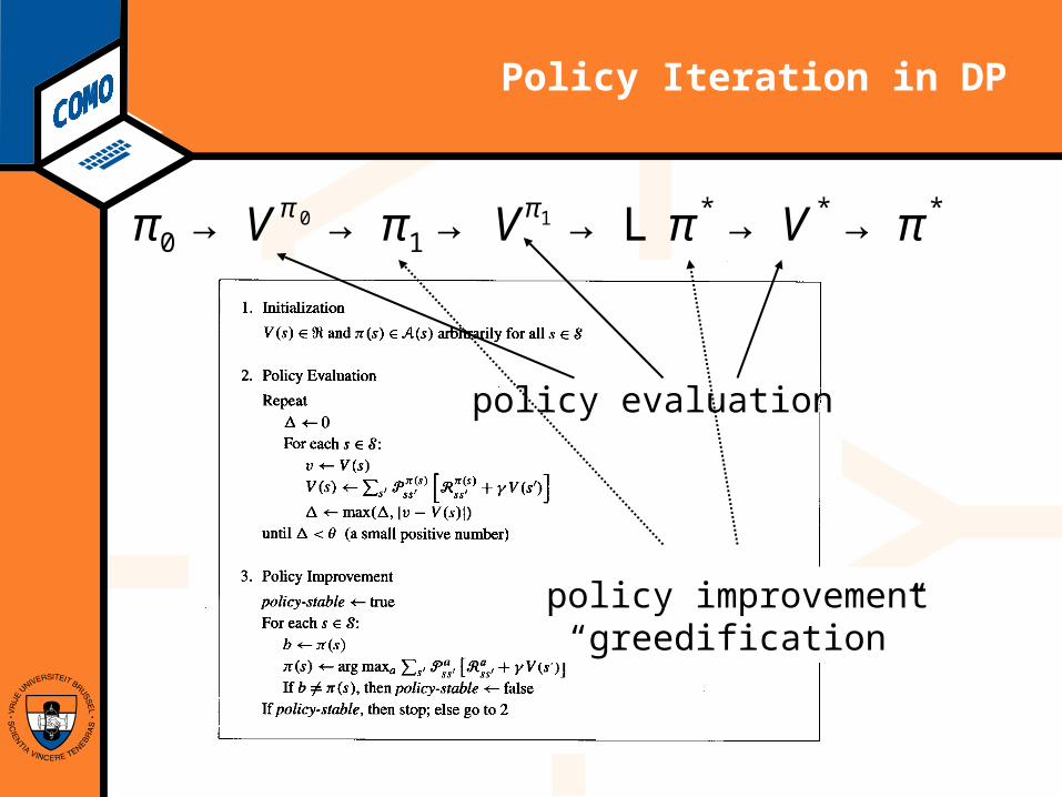
Policy Iteration in DP
π0 → Vπ0 → π1 → Vπ1 → L π* → V* → π*
policy improvement“greedification”
policy evaluation
Computational Modeling Lab
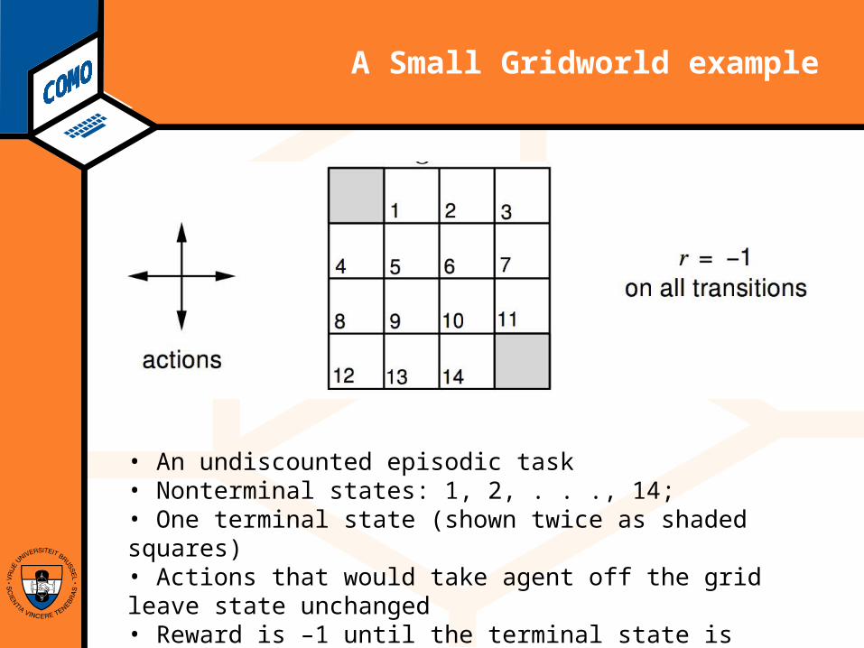
A Small Gridworld example
• An undiscounted episodic task• Nonterminal states: 1, 2, . . ., 14; • One terminal state (shown twice as shaded squares)• Actions that would take agent off the grid leave state unchanged• Reward is –1 until the terminal state is reached• is set to 1
Computational Modeling Lab
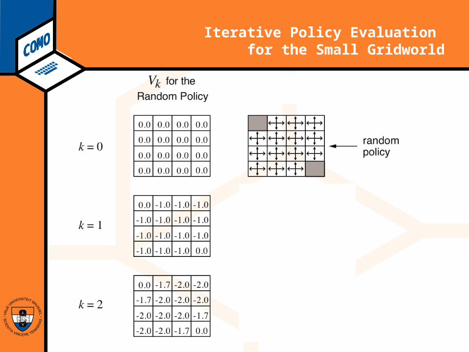
Iterative Policy Evaluation for the Small Gridworld
Computational Modeling Lab
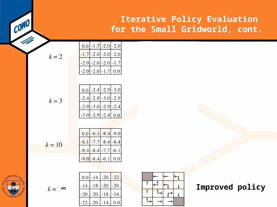
Iterative Policy Evaluation for the Small Gridworld, cont.
Improved policy∞
Computational Modeling Lab
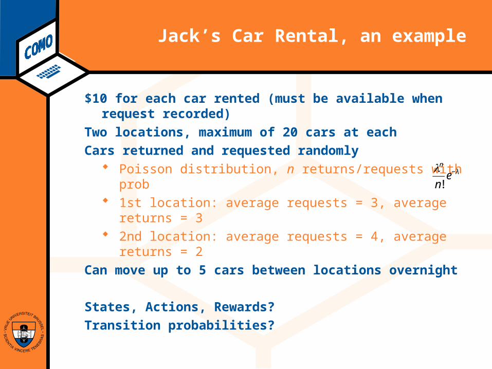
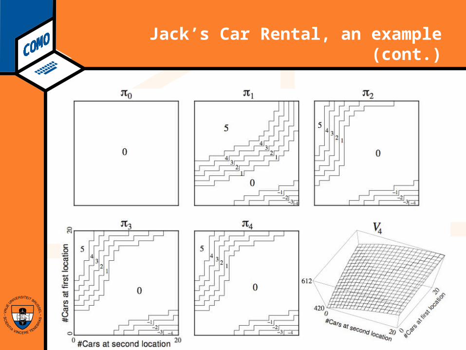
Jack’s Car Rental, an example
$10 for each car rented (must be available when request recorded)
Two locations, maximum of 20 cars at eachCars returned and requested randomly
Poisson distribution, n returns/requests with prob 1st location: average requests = 3, average returns
= 3 2nd location: average requests = 4, average returns
= 2Can move up to 5 cars between locations overnight
States, Actions, Rewards?Transition probabilities?
€
λn
n!e−λ
Computational Modeling Lab
Jack’s Car Rental, an example (cont.)
€
λn
n!e−λ
Computational Modeling Lab
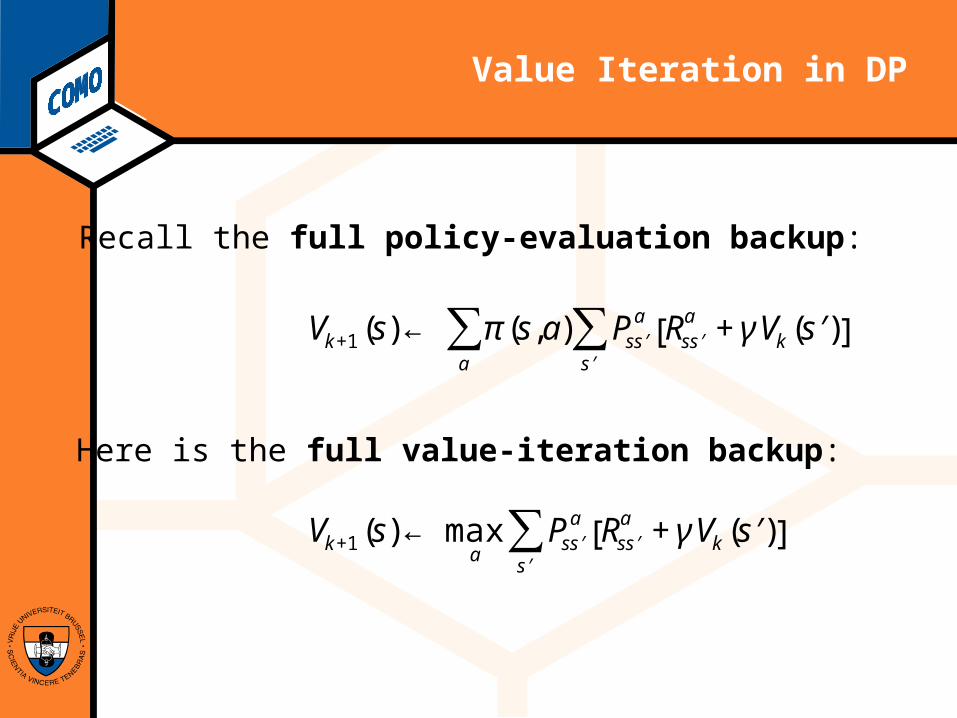
Value Iteration in DP
Vk+1(s)← π(s,a) Ps ′ s a Rs ′ s
a +γVk( ′ s )[ ]′ s
∑a∑
Recall the full policy-evaluation backup:
Vk+1(s)← maxa
Ps ′ s a Rs ′ s
a +γVk( ′ s )[ ]′ s
∑
Here is the full value-iteration backup:
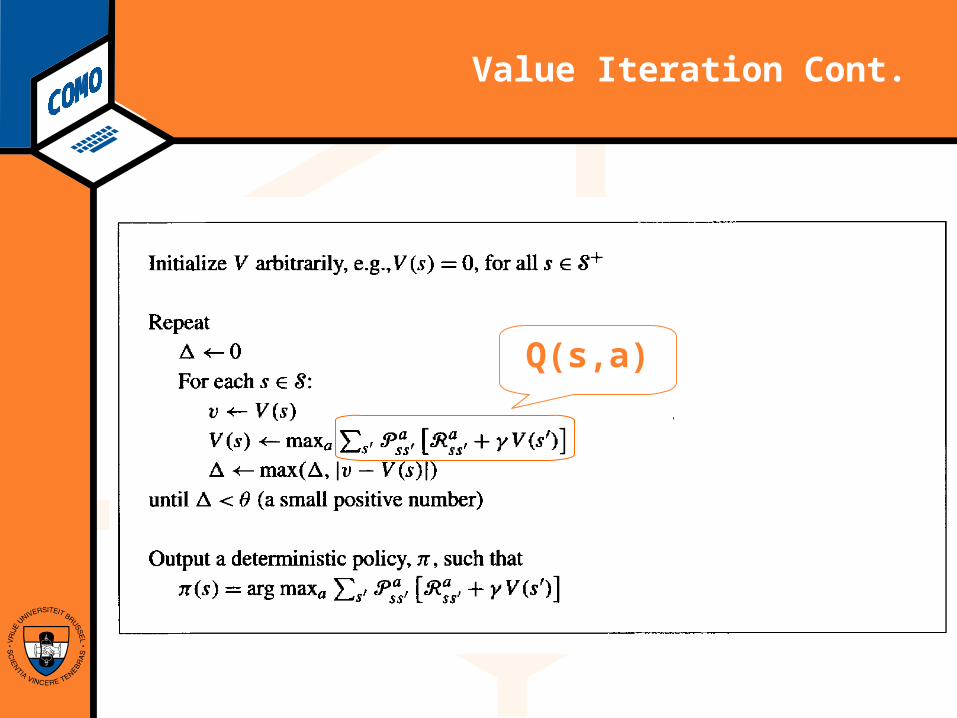
Computational Modeling Lab
Value Iteration Cont.
Q(s,a)
Computational Modeling Lab
Asynchronous DP
All the DP methods described so far require exhaustive sweeps of the entire state set.
Asynchronous DP does not use sweeps. Instead it works like this:
Repeat until convergence criterion is met:
Pick a state at random and apply the appropriate backup
Still need lots of computation, but does not get locked into hopelessly long sweeps
Can you select states to backup intelligently? YES: an agent’s experience can act as a guide.
Computational Modeling Lab
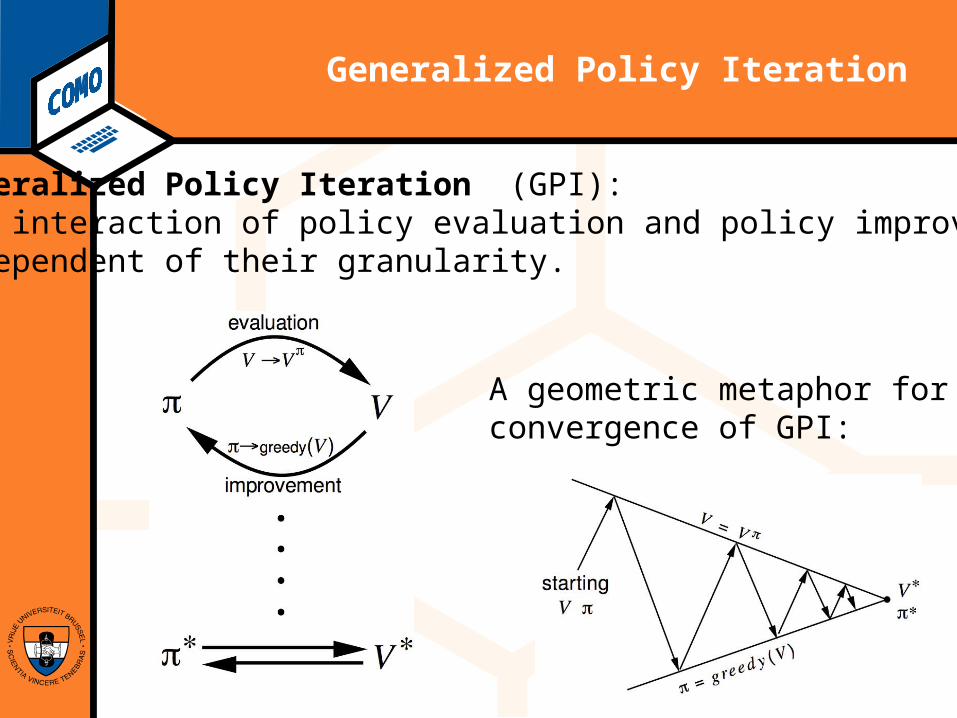
Generalized Policy Iteration
Generalized Policy Iteration (GPI): any interaction of policy evaluation and policy improvement, independent of their granularity.
A geometric metaphor forconvergence of GPI:
Computational Modeling Lab
Efficiency of DP
To find an optimal policy is polynomial in the number of states…
BUT, the number of states is often astronomical, e.g., often growing exponentially with the number of state variables (what Bellman called “the curse of dimensionality”).
In practice, classical DP can be applied to problems with a few millions of states.
Asynchronous DP can be applied to larger problems, and appropriate for parallel computation.
It is surprisingly easy to come up with MDPs for which DP methods are not practical.
Computational Modeling Lab
Summary
• Policy evaluation: backups without a max
• Policy improvement: form a greedy policy, if only locally
• Policy iteration: alternate the above two processes
• Value iteration: backups with a max• Generalized Policy Iteration (GPI)• Asynchronous DP: a way to avoid
exhaustive sweeps