Embed Size (px)
Citation preview

Computational Methods in
Nondestructive Evaluation (NDE)
for Damage State Characterization
Mark Blodgett (PI), Jeremy Knopp, and John Aldrin
AFRL/RXLP
AFOSR Structural Mechanics
Annual Review
24-27 July 2012
AFOSR Program Manager: Dr. David Stargel

Computational Methods in NDE for Damage State Characterization
Challenge: Address Wide Variability and Uncertainty in NDE
Measurements, Part Geometry, Material Systems,
Flaw Characteristics and Environmental Factors
Problem: Characterize Cracks at Fastener Sites
Using Ultrasonic and Eddy Current NDE
Sensors
(Arrays)
Advanced
Models
Model-based
Inverse Methods
for Material State
Estimation
• multiscale damage characterization
• material properties measurement
Model-assisted
POD Assessment
NDE
Validation
Integrated
Probabilistic Models
• NDE/SHM
• life prediction
• risk assessment
• cost-benefit analysis
Optimal Service
Life Management
(Digital Twin)
Improve NDE Sensitivity / Characterization
(Depth, Small Cracks, Sizing) Payoff:
0 0.02 0.04 0.06 0.08 0.1 0.12 0.14 0.16 0.18 0.20
0.1
0.2
0.3
0.4
0.5
0.6
0.7
0.8
0.9
1
crack length (in)
PO
D
MAPOD
exp.
Approach (FY11):
Forward problems Inverse problems Mixed simulated
and empirical
evaluations
Efficient Methods for Propagating
Parameter Variability and Uncertainty

Objective (FY11-13)
Objective: To develop NDE characterization methods for damage in aircraft
structures and engine components using mechanical stress and
electromagnetic waves that integrate the development and
implementation of advanced computational methods
Proposed Research on New Capabilities:
• Efficient methods for propagating parameter variability and
uncertainty for forward problems in NDE,
• Statistical validation metrics incorporating stochastic
methods for robust inverse methods design,
(model-assisted POD / reliability assessment)
• Model-based crack characterization in aerospace applications,
• Develop model-based damage characterization and data fusion
methods for complex structural inspection problems,
• Integrate and optimize algorithms with emerging array sensor
technologies (MR arrays, 2D ultrasonic phased arrays)

Highlights - FY12
• Efficient methods for propagating parameter variability and uncertainty for
forward problems in NDE,
• PCM foundational methods
• KL-transform / ANOVA
• Smolyak Sparse grids
• Statistical validation metrics incorporating stochastic methods for robust
inverse methods design, (model-assisted POD / reliability assessment)
• Bayesian method in POD / MAPOD evaluation
• Traditional methods re-examined with Bayesian Tools
• Box-Cox / Bootstrap
• Physics-inspired model evaluations
• Bayesian POD model and uncertain parameter estimation (e.g. aspect ratio)
• Discussion of metrics for inverse methods (GP models)
• Model-based crack characterization in aerospace applications,
• Case studies for surface-breaking cracks [transition]
• Prelim. emerging array sensor technologies (MR arrays)

Uncertainty Propagation
• Motivation: Model evaluations are computationally expensive. There is a need for more efficient methods than Monte Carlo
• Objective: Efficiently propagate uncertain inputs through “black box” models and predict output probability density functions. (Non-intrusive approach)
• Approach: Surrogate models based on Polynomial Chaos Expansions meet this need.
Eddy Current NDE Model
[Deterministic]
n
2
1
Z~
UniformX
NormalX
n ~
~1
Eddy Current NDE Model
[Stochastic] ? ~
~Z
Input Parameters with Variation:
• Probe dimensions
(Liftoff / tilt)
• Flaw characteristics
(depth, length, shape)

Uncertainty Propagation
Uncertainty propagation for parametric NDE characterization problems:
• Probabilistic Collocation Method (PCM) approximates model
response with a polynomial function of the uncertain parameters.
• This reduced form model can then be used with
traditional uncertainty analysis approaches,
such as Monte Carlo.
Extensions of generalized polynomial chaos (gPC) to high-dimensional
(2D, 3D) damage characterization problems:
• Karhunen-Loeve expansion
• Analysis of variance (ANOVA)
• Smolyak Sparse Grids
N
Number of Unknowns
to Evaluate
1
Critical
Flaw Size
Key Damage and
Measurement
States (e.g. crack
length, probe liftoff)
Parameterized
Flaw
Localization
and Sizing
Full 3D
Damage and
Material State
Characterization
>1 >>1
N
i
iicfZ1
)()(ˆ xx

Approach (1): Karhunen-Loeve Expansion
• Address stochastic input variable reduction when number of
random variables (N) is large.
• Apply Karhunen-Loeve Expansion to map random variables into
a lower-dimensional random space (N').
Eddy Current Example:
• Correlation function (covariance model)
defines random conductivity map,
• Set choice of grid length to
– achieve model convergence and
– eliminate insignificant eigenvalues
for reduced order conductivity map.
Uncertainty Propagation and High Dimensional Model Representation
N
n
nnn
1
)()( xx )(x Karhunen-
Loéve
Expansion
N ...1
covariance
model
),( xx C
conductivity map with
N random variables
reduced order conductivity map
with N' random variables
N' random variables
Crystallites
(Grains)
=2.2*106 S/m
Coil

Approach (2): Analysis of Variance (ANOVA) Expansion
• Provides surrogate to represent high dimensional set of parameters
• Analogous to ANOVA decomposition in statistics
• Locally represent model output through
expansion at anchor point in -space
– Requires inverse problem
– Replace random surface with
equivalent 'homogeneous' surface
Uncertainty Propagation and High Dimensional Model Representation
ANOVA Expansion
N
n
nnn
1
)()( xx )(x Karhunen-
Loéve Expansion
N ...1
defined by
covariance
model
),( xx C
conductivity
map with
N random
variables
reduced order
conductivity map with
N' random variables
N' random variables (1) Identify
unique
sources
of variance
(2) Identify
significant
factors
in model M ...1
M random variables
)(ξZ
N' >> M N >> N' ξξ

Approach (2): Analysis of Variance Expansion + Smolyak Sparse Grids
• Significant computational expense for high-dimensional integrals
• Can leverage sparse grids based on the Smolyak construction
[Smolyak, 1963; Xiu, 2010; Gao and Hesthaven, 2010]
– Provides weighted solutions at specific nodes and adds them to
reduce the amount of necessary solutions
– Sparse grid collocation provides subset of full
tensor grid for higher dimensional problems
– Approach can also be applied to gPC/PCM
Uncertainty Propagation and High Dimensional Model Representation
ANOVA Expansion
N
n
nnn
1
)()( xx )(x Karhunen-
Loéve Expansion
N ...1
defined by
covariance
model
),( xx C
conductivity
map with
N random
variables
reduced order
conductivity map with
N' random variables
N' random variables (1) Identify
unique
sources
of variance
(2) Identify
significant
factors
in model M ...1
M random variables
)(ξZ
N' >> M N >> N' ξξ
-1 -0.5 0 0.5 1-1
-0.5
0
0.5
1Sparse Grid and Full Tensor Product Grid

Bayes Factor in Hit-miss POD Evaluation
Example (1) [NTIAC 9002(3)L]:
• Application of wrong model with poor data
Approach: Investigate more sophisticated statistical models and
Bayes Factor for model evaluation and selection procedures
0
10
20
30
40
50
60
70
80
90
100
0
10
20
30
40
50
60
70
80
90
100
-0.05 0.00 0.05 0.10 0.15 0.20 0.25 0.30 0.35 0.40 0.45 0.50 0.55 0.60 0.65 0.70 0.75PR
OB
AB
ILIT
Y O
F D
ET
EC
TIO
N (
%)
ACTUAL CRACK LENGTH - (Inch)
Data Set: A9002(3)L
Test Object : 2219
Aluminum,
Stringer
Stiffened Panels
Condition: After Etch
Method: Eddy Current,
Raster
Scan with
NTIAC, Nondestructive Evaluation (NDE) Capabilities Data Book 3rd ed., NTIAC DB-97-02, Nondestructive Testing Information Analysis
Center, November 1997

0 2 4 6 8 10 12 14 16 18 200
0.1
0.2
0.3
0.4
0.5
0.6
0.7
0.8
0.9
1
0 2 4 6 8 10 12 14 16 18 200
0.1
0.2
0.3
0.4
0.5
0.6
0.7
0.8
0.9
1
Bayes Factor in Hit-miss POD Evaluation
• Summary of Marginal Likelihood (ML) Results
Using Bayes Factor for POD Model Fits
a (mm)
â
0 2 4 6 8 10 12 14 16 18 200
0.1
0.2
0.3
0.4
0.5
0.6
0.7
0.8
0.9
1
0 2 4 6 8 10 12 14 16 18 200
0.1
0.2
0.3
0.4
0.5
0.6
0.7
0.8
0.9
1
2 parameter Probit 3 parameter
lower bound Probit
4 parameter Probit
(most likely)
3 parameter
upper bound Probit
ML
2 parameter Logit 3.70E-97
2 parameter Probit 9.08E-98
3 parameter lower bound Logit 7.29E-98
3 parameter lower bound Probit 1.02E-98
3 parameter upper bound Logit 3.27E-93
3 parameter upper bound Probit 1.64E-93
4 parameter Logit 7.24E-92
4 parameter Probit 2.49E-92
a (mm)
â
a (mm)
â
Knopp, J. and Zeng. L., “Statistical Analysis of Hit/Miss Data,” Materials Evaluation (submitted, 2012).

Box-Cox Transformations
• POD response data analysis (â vs a) assumes
homoscedasticity, and if that assumption is violated,
one must resort to hit/miss analysis. This was the
case for an early MAPOD study (Knopp 2007)
• Box-Cox transformation can remedy this problem.
0 1 2 3 4 5
-0.02
0.00
0.02
0.04
0.06
0.08
0.10
sig
na
l re
sp
on
se
â
crack size (mm)
• Power transformation
• Common transformations
ââ
22ââ
5.0 ââ
0 ââ elog
5.0â
â1
0.1â
â1

Box-Cox Transformations
• Box-Cox enables â vs a analysis for data sets where
the variance is not constant but has some relationship
with the independent variable such as crack size.
analysis
method
λ left
censor
detection
threshold
false
calls
a90 (mm) a90/95 (mm) a90 - a90/95 %
difference
1st order
linear
0.45 0.13 0.23 0 2.176 2.327 6.9%
1st order
linear
0.5 0.14 0.195 1 2.102 2.257 7.3%
1st order
linear
0.5 0.195 0.195 1 2.269 2.53 11.5%
2nd order
linear
0.5 .14 0.195 1 2.277 2.472 8.5%
2nd order
linear
0.5 0.195 0.195 1 2.197 2.428 10.5%
hit/miss 1 0.187 1 1.72 2.04 18.6%
hit/miss 1 0.162 11 1.498 1.907 27.3%

Physics-inspired Models and Confidence Bound Evaluation
• Visual inspection reveals that a 2nd order
linear model may fit the data better than
the standard „â vs a‟ analysis.
• Evidence: p-value for a2 is 0.001 and
adjusted R-square value increases
slightly with inclusion of a2.
• Confidence bounds calculation on models more complicated than
„â vs a‟, especially transforming to probability of detection curve.
• Bootstrap methods are simple and flexible enough to provide
confidence bounds for a wide variety of models.
• Example for the previous
transformed data set with
λ = 0.5
– Results for a90 and a90/95
values converge well
-0.5 0.0 0.5 1.0 1.5 2.0 2.5 3.0 3.5 4.0 4.5 5.0
-0.02
0.00
0.02
0.04
0.06
0.08
0.10
-0.5 0.0 0.5 1.0 1.5 2.0 2.5 3.0 3.5 4.0 4.5 5.0
-0.02
0.00
0.02
0.04
0.06
0.08
0.10
Experiment
Simulation
a90 a90/95
Wald Method 2.102 mm 2.257 mm
Bootstrap 1,000 2.096 mm 2.281 mm
Bootstrap 10,000 2.099 mm 2.299 mm
Bootstrap 100,000 2.099 mm 2.297 mm

0 0.02 0.04 0.06 0.08 0.1 0.12 0.14 0.16 0.18-0.05
0
0.05
0.1
0.15
a1 (in.)
ahat
0 0.02 0.04 0.06 0.08 0.1 0.12 0.14 0.16 0.18-0.1
-0.05
0
0.05
0.1
a1 (in.)
resid
uals
0 0.02 0.04 0.06 0.08 0.1 0.12 0.14 0.16 0.180
0.5
1
a1 (in.)
PO
D
POD: physics-based model, Bayes/MCMC
• Example: Eddy Current Inspection of Cracks at Fastener Sites
• Case Study for Physics-based Model Evaluation:
•
• where f () is a function call for a physics-based model (i.e. VIC-3D)
• Bayesian POD Analysis Performed in Matlab + R:
• MCMC library in Matlab used for Bayesian Analysis
• Matlab Provides Option for Integration of Model Function in Bayesian Fit
• Compare Ahat-vs-a fit (MLE, Wald bounds) and a Physics-based Model Fit
Bayesian Methods with Physics-based Model POD / MAPOD Evaluation (1)
2110 ,ˆ aafa
zb
a
0 0.02 0.04 0.06 0.08 0.1 0.12 0.14 0.16 0.18-0.05
0
0.05
0.1
0.15
a1 (in.)
ahat
0 0.02 0.04 0.06 0.08 0.1 0.12 0.14 0.16 0.18-0.04
-0.02
0
0.02
0.04
a1 (in.)
resid
uals
0 0.02 0.04 0.06 0.08 0.1 0.12 0.14 0.16 0.180
0.5
1
a1 (in.)
PO
D
POD: ahat-vs-a model, MLE+WaldAhat-vs-a fit (MLE, Wald bounds) Physics-based model fit (Bayes/MCMC)
Physics-based
Model Fit
Provides
Better Match
and
Residuals Are
Reduced
),0(~ 2
N

0 0.02 0.04 0.06 0.08 0.1 0.12 0.14 0.16 0.18-0.05
0
0.05
0.1
0.15
a1 (in.)
ahat
0 0.02 0.04 0.06 0.08 0.1 0.12 0.14 0.16 0.18-0.1
-0.05
0
0.05
0.1
a1 (in.)
resid
uals
0 0.02 0.04 0.06 0.08 0.1 0.12 0.14 0.16 0.180
0.5
1
a1 (in.)
PO
D
POD: physics-based model, Bayes/MCMC
0 0.02 0.04 0.06 0.08 0.1 0.12 0.14 0.16 0.18-0.05
0
0.05
0.1
0.15
a1 (in.)
ahat
0 0.02 0.04 0.06 0.08 0.1 0.12 0.14 0.16 0.18-0.1
-0.05
0
0.05
0.1
a1 (in.)
resid
uals
0 0.02 0.04 0.06 0.08 0.1 0.12 0.14 0.16 0.180
0.5
1
a1 (in.)
PO
D
POD: physics-based model, Bayes/MCMC
0 0.02 0.04 0.06 0.08 0.1 0.12 0.14 0.16 0.18-0.05
0
0.05
0.1
0.15
a1 (in.)
ahat
0 0.02 0.04 0.06 0.08 0.1 0.12 0.14 0.16 0.18-0.04
-0.02
0
0.02
0.04
a1 (in.)
resid
uals
0 0.02 0.04 0.06 0.08 0.1 0.12 0.14 0.16 0.180
0.5
1
a1 (in.)
PO
D
POD: ahat-vs-a model, MLE+Wald
• Example: Eddy Current Inspection of Cracks at Fastener Sites
• Case Study for Physics-based Model Evaluation:
•
• where f () is a function call for a physics-based model (i.e. VIC-3D)
• Bayesian POD Analysis Performed in Matlab + R:
• MCMC library in Matlab used for Bayesian Analysis
• Matlab Provides Option for Integration of Model Function in Bayesian Fit
• Compare Ahat-vs-a fit (MLE, Wald bounds) and a Physics-based Model Fit
2110 ,ˆ aafa
zb
a
0 0.02 0.04 0.06 0.08 0.1 0.12 0.14 0.16 0.18-0.05
0
0.05
0.1
0.15
a1 (in.)
ahat
0 0.02 0.04 0.06 0.08 0.1 0.12 0.14 0.16 0.18-0.04
-0.02
0
0.02
0.04
a1 (in.)
resid
uals
0 0.02 0.04 0.06 0.08 0.1 0.12 0.14 0.16 0.180
0.5
1
a1 (in.)
PO
D
POD: ahat-vs-a model, MLE+Wald
Ahat-vs-a fit (MLE, Wald bounds) Physics-based model fit (Bayes/MCMC)
Result is
More Accurate
Representation
of the Data in
the POD Model
Fit
),0(~ 2
N
Bayesian Methods with Physics-based Model POD / MAPOD Evaluation (1)

0.496 0.498 0.5 0.502 0.504 0.506 0.5080
2000
4000
6000
8000
theta1 (bias)
6.5 7 7.5 8 8.5 9 9.5 100
2000
4000
6000
theta2 (slope)
0.8 0.85 0.9 0.95 1 1.05 1.1 1.15 1.2 1.250
2000
4000
6000
1/theta3 (aspect ratio: a/b)
0 0.02 0.04 0.06 0.08 0.1 0.12 0.14 0.16 0.18-0.05
0
0.05
0.1
0.15
a1 (in.)
ahat
0 0.02 0.04 0.06 0.08 0.1 0.12 0.14 0.16 0.18-0.1
-0.05
0
0.05
0.1
a1 (in.)
resid
uals
0 0.02 0.04 0.06 0.08 0.1 0.12 0.14 0.16 0.180
0.5
1
a1 (in.)
PO
D
POD: physics-based model, Bayes/MCMC
• Example: Eddy Current Inspection of Cracks at Fastener Sites
• Case Study for Physics-based Model Evaluation:
•
• where f () is a function call for a physics-based model
• 0 , 1 = model calibration parameters
• 2 = random variable associated with crack aspect ratio (b/a)
• 3 = random variable associated with liftoff variation
• Results: Fit POD Model and Estimate of Variation in Aspect Ratio
[use non-informative priors]
• Issues with „Naïve‟ Approach:
• Need true estimate of variance for
crack aspect ratio random variable
→ Use hierarchical models
• Address correlated / confounded
parameters in estimation problem
→ Use informative priors and
constraints from expert opinion
32110 ,;ˆ afa
zb
a
),0(~ 2
N
Bayesian Methods with Physics-based Model POD / MAPOD Evaluation (2)

0 0.05 0.1 0.15 0.2-0.1
0
0.1
0.2
0.3
a1 (in.)
ahat
• Example: Eddy Current Inspection of Cracks at Fastener Sites
• Challenge: Address non-constant variance wrt flaw size
• Hierarchical NDE Measurement Models:
•
• where f () is a function call for a physics-based model
• 0 , 1 = model calibration parameters
• h = random variable (varying-slope model)
• 2h = variance in slope parameter
• 2 = random variable associated
with crack aspect ratio (b/a)
• 2h = variance in slope parameter
• Simple Test Case: Fit data from model with varying slope >> noise.
Hierarchical Models for Estimating Variance of a Random Variable
aaa ˆ110ˆ h
zb
a
),0(~ 2
ˆˆ aa N
1st
2nd
aafa ˆ2110 ;ˆ
hh ),0(~ 2
hh N ),(~ 2
2 22 N);,0(~ 2
ˆˆ aa N
physics-based model statistical model
• A. Gelman, J. B. Carlin, H. S. Stern, and D. B. Rubin, Bayesian Data Analysis, 2003.
• A. Gelman and J. Hill, Data Analysis Using Regression and Multilevel/Hierarchical Models, 2007.

• Simple Test Case: Fit data from model with varying slope >> noise.
• Hierarchical NDE Measurement Models:
• Results: Ns = 100
Hierarchical Models for Estimating Variance of a Random Variable
aaa ˆ110ˆ h ),0(~ 2
ˆˆ aa N
hh ),0(~ 2
hh N
Ns = 100 0 1 h
True Value 0.0000 1.0000 0.3000 0.00100
WinBUGS
Mean -0.00024 1.0312 0.2580 0.00139
95% Credible Bds (-0.00119,0.00364) (0.9848,1.0810) (0.2286,0.2923) (0.00103,0.00210)
Matlab
Mean -0.00027 1.0361 0.2768 0.01166
95% Credible Bds (-0.00418,0.00071) (0.9862,1.0863) (0.2593,0.2974) (0.01012,0.01346)
0 0.02 0.04 0.06 0.08 0.1 0.12 0.14 0.16 0.18 0.20
0.05
0.1
0.15
0.2
0.25
a1 (in.)
ahat

Bayesian Methods - Challenges
Uncertainty Quantification (UQ) community developing Bayesian framework
for the use of computational models with observational data
• SAMSI program on UQ (2012):
• SIAM UQ conference 2012: http://www.siam.org/meetings/uq12/
Key Insight / Research Directions:
• 1) Must include model discrepancy and not treat it as random error.
• Calibrating (inverting, tuning) a wrong model gives parameter estimates
that are wrong (not equal to their true physical values) [O‟Hagan, 2012]
• Gaussian Process (GP) models typically used to fit model discrepancy
[Kennedy/O‟Hagan 2002].
• 2) Use of prior information in Bayesian framework can greatly help.
• To learn about model parameters in the presence of discrepancy, better
prior information is needed [Bayarri, 2012]
• Elicitation of expert opinion is an active research topic [O‟Hagan, 2012]
• 3) Should leverage model form uncertainty (assessment) approaches.
• To identify best models and address limitations cited by UQ community
[Grandhi et al, Wright State University]

Compare NDE „Ahat-vs-a‟ POD and NDE Characterization Error (CE) Evaluations
Characterization Error Analysis:
• Build on Protocol for NDE/SHM
• Perform evaluation studies
• experimental sizing results
• simulated sizing results
• Evaluate characterization error
(êj) with respect to flaw size (ak)
• error model (êj= âj - aj)
• uncertainty bounds
Ahat-vs-A POD Analysis:
• Follow MIL-HDBK 1823A
• Perform evaluation studies
• experimental measurements
• simulated measurements
• Evaluate model of measurement
(âj) with respect to flaw size (ak)
• mean model
• confidence (uncert.) bounds
a1
â
a1
ê1

Model-assisted Process (Tools) for NDE Characterization Error (CE) Evaluation
2) Model-based
Uncertainty
Propagation
Model
Error
Input Parameter
Variability
(Distributions)
Stochastic
Models
Model
„Calibration„
(Error)
3) Revise Model Estimates
with Experimental Data
Using Bayesian Methods
Confidence Bounds
(Limited Samples)
Challenge: This is Complicated. Must Focus on Key Drivers of Error. [Annis]
Characterization Error
w/Uncertainty Bounds
1) Assess Key
Factors (Joint PDFs)
of Inversion Process
Build Experimental
Adjustments to
êj vs. ak
Build Theoretical
Adjustments to
êj vs. ak
Bayesian Methods:
Estimate unknown / uncertain
joint parameter distributions
Stochastic Numerical
Methods:
- Prob. Collocation Method
- KL Transform + ANOVA
Gaussian Processes:
Represent range of random
variables with multivariate
normal distribution
Bayesian Calibration:
Revise model (GP) using
Bayesian method with
Empirical model / data

Gaussian Process (GP)
• A Gaussian Process is a collection of random variables
with the property that the joint distribution of any finite
subset is a Gaussian function. It consists of:
– Mean function (model)
– Covariance function
– Learning equates to finding suitable
properties for the covariance function
– Hyperparameters: smoothness, characteristic length scales
[From MacKey, 2006,
“Gaussian Process Basics”]
0 0.02 0.04 0.06 0.08 0.1 0.12 0.14 0.16 0.18-0.02
0
0.02
0.04
0.06
0.08
0.1
0.12
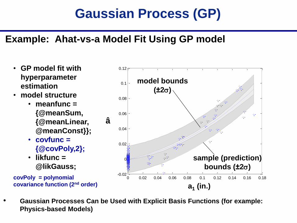
Gaussian Process (GP)
Example: Ahat-vs-a Model Fit Using GP model
• GP model fit with
hyperparameter
estimation
• model structure
• meanfunc =
{@meanSum,
{@meanLinear,
@meanConst}};
• covfunc =
{@covPoly,2};
• likfunc =
@likGauss;
a1 (in.)
sample (prediction)
bounds (±2)
model bounds
(±2)
• Gaussian Processes Can be Used with Explicit Basis Functions (for example:
Physics-based Models)
â
covPoly = polynomial
covariance function (2nd order)

Model-based Crack Characterization in Aerospace Applications
To characterize a fatigue crack condition around a fastener site
through model-based damage characterization approaches,
a number of conditions must be simultaneously estimated:
Crack dimensions (a, b)
Crack location (z, q)
NDE source and sensor (EC, UT)
position and orientation (xk ,l )
Fastener and crack contact conditions (ai, j)
Morphology and residual stress across crack face
Enabling Technologies to Achieve Objectives:
• Model-based inverse methods (with validated model through benchmark studies)
• Efficient stochastic models addressing varying and uncertain conditions
• To evaluate the sensitivity of the inverse methods
• To optimize the design of the NDE procedure
• Discovery of ‘invariant‟ NDE data features (insensitive to varying conditions)
• Bayesian inverse methods (address refinement using a priori information)

Publications (FY12)
• Knopp, J., and Zeng, L., “Statistical Analysis of Hit/Miss Data”, Materials Evaluation, (submitted, 2012.)
• Knopp, J., Grandhi, R., Aldrin, J. C., Park, I., “Statistical Analysis of Eddy Current Data from Fastener
Site Inspections,” Journal of Nondestructive Evaluation, (submitted, 2012.)
• Aldrin, J. C., Knopp, J., Sabbagh, H. A., “Bayesian Methods in Probability of Detection Estimation and
Model-assisted Probability of Detection (MAPOD) Evaluation,” Review of Progress in QNDE, Vol. 31,
AIP, (to be published, 2013).
• Cherry, M. and Knopp, J., “Stochastic Collocation Method for Higher Dimensional NDE Problems with
Tensor Product Grids”, Review of Progress in QNDE, Vol. 31, AIP, (to be published, 2013).
• Aldrin, J. C., Knopp, J., “False Call Rate Estimation,” Review of Progress in QNDE, Vol. 31, AIP, (to be
published, 2013).
• Aldrin, J. C., Sabbagh, H. A., Murphy, R. K., Sabbagh, E. H., Knopp, J. S., Lindgren, E. A., Cherry, M.
R., “Demonstration of model-assisted probability of detection evaluation methodology for eddy current
nondestructive evaluation,” Review of Progress in QNDE, Vol. 31, AIP, pp.1733-1740, (2012).
• Aldrin, J. C., Medina, E. A., Santiago, J., Lindgren, E. A., Buynak, C., Knopp, J., “Demonstration study
for reliability assessment of SHM systems incorporating model-assisted probability of detection
approach,” Review of Progress in QNDE, Vol. 31, AIP, pp.1543-1550, (2012).
• Sabbagh, H. A., Murphy, R. K., Sabbagh, E. H., Aldrin, J. C., Knopp, J., Blodgett, M. P., “Stochastic-
integral models for propagation-of-uncertainty problems in nondestructive evaluation,” The 28th Annual
Review of Progress in Applied Computational Electromagnetics Society (ACES), Columbus, OH, (2012).
• F. Kojima, J. S. Knopp, "Inverse Problem for Electromagnetic Propagation in a Dielectric Medium using
Markov Chain Monte Carlo Method", International Journal of Innovative Computing Information and
Control, vol 8 (3), pp. 2339-2346, (2012) (Note: AOARD grant FA2386-10-1-4076)