Embed Size (px)
Citation preview
Computational Geometry Seminar Lecture 1
Drawing Planar Graphs
2
Graph
• Definition: A Simple Undirected Graph G consists of:
A finite set of vertices V(G).
A set E(G) of sets of 2 vertices, called edges.
• Note: From now on we will call this type of graphs by the general name Graph.
3
Degree
• Definition: In a graph G, the vertices u, v are adjacent iff the edge uv belongs to E(G).
• The number of adjacent vertices to a vertex u is called the degree of u, denoted d(u).

4
Subgraph
• Definition: A graph H is a subgraph G (written H G) iff V(H) V(G) and E(H) E(G).
• We say that a graph H is the subgraph of G induced by a set of vertices U V(G) if V(H) = U and E(H) is the set of all the edges of G connecting vertices of U.
5
Paths and Cycles
• Definition: A sequence of k distinct vertices, in which every consecutive vertices are adjacent, is called a path of length k-1.
• Definition: A path of length k-1 with the addition of an edge from the last vertex to the first vertex of the path is called a cycle of length k.
6
Connectivity
• Definition: A maximal set of vertices, for which there exists a path from every vertex in the set to another, is called a connected component.
• A graph composed of only one connected component is called connected.
7
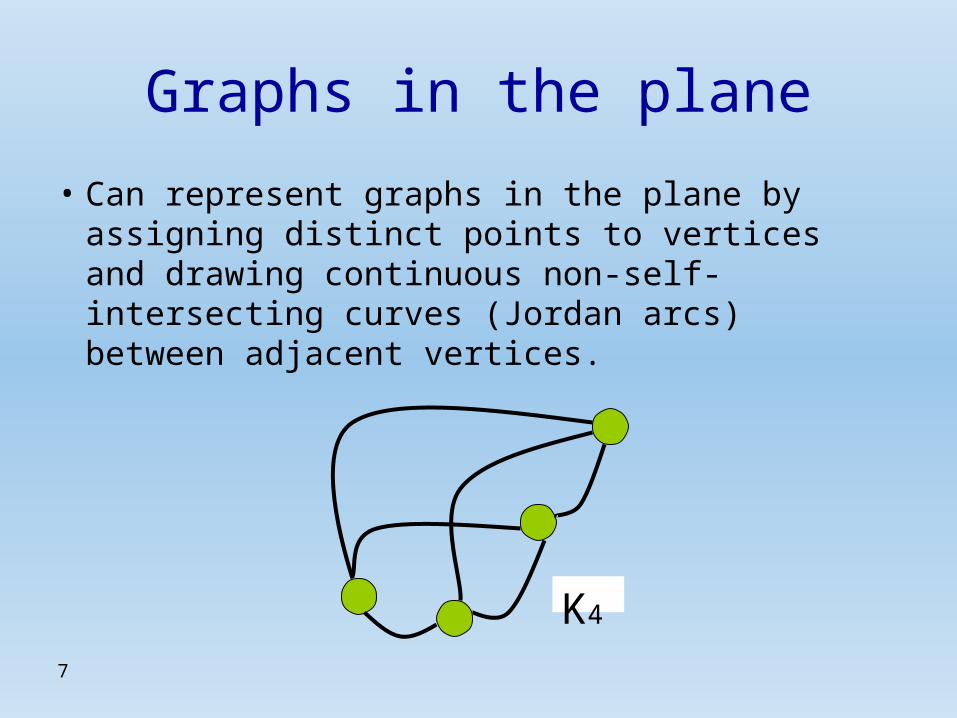
Graphs in the plane
• Can represent graphs in the plane by assigning distinct points to vertices and drawing continuous non-self-intersecting curves (Jordan arcs) between adjacent vertices.
K4
8
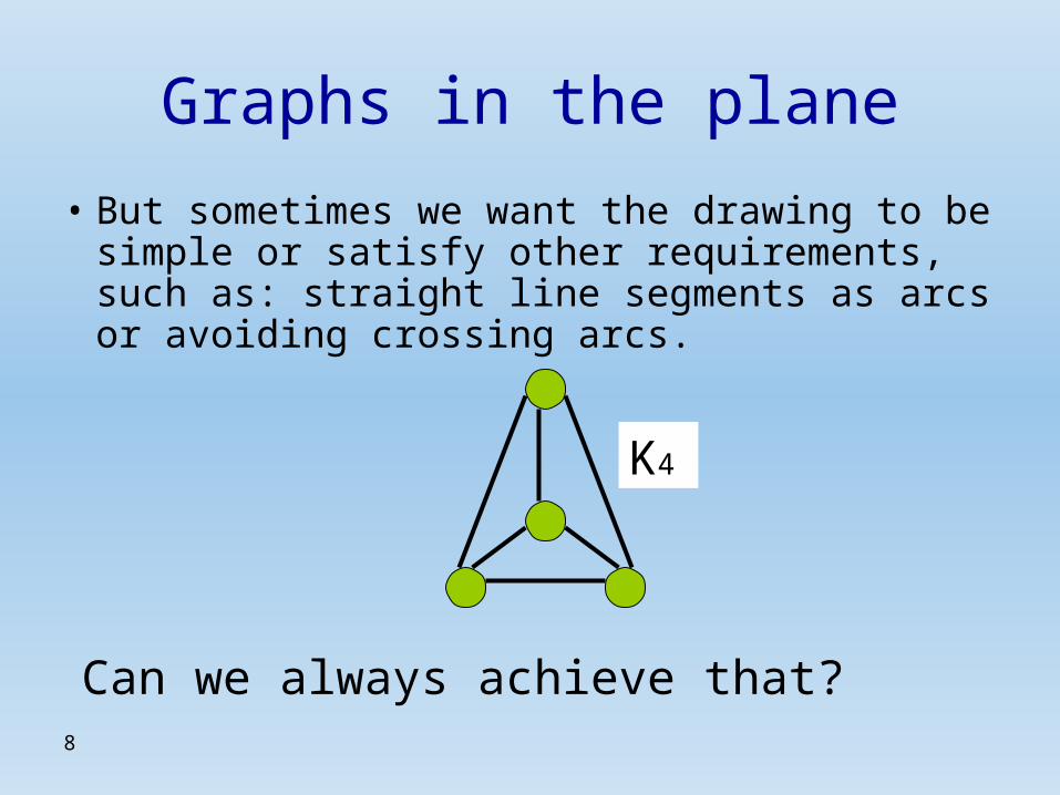
Graphs in the plane
• But sometimes we want the drawing to be simple or satisfy other requirements, such as: straight line segments as arcs or avoiding crossing arcs.
K4
Can we always achieve that?
9
Planar Graphs
• Definition: A graph that can be represented in the plane so that no two arcs meet at a point other than their endpoints is called a Planar graph.
• Such representation of a planar graph is called a Plane graph or Planar embedding of the graph.
10
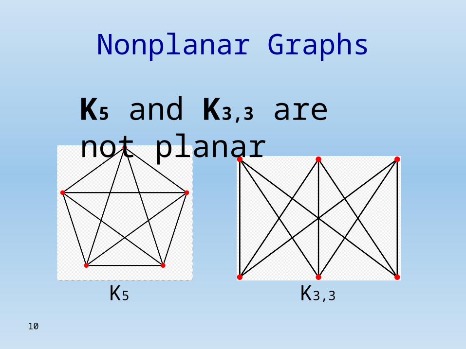
Nonplanar Graphs
K5 K3,3
K5 and K3,3 are not planar
11
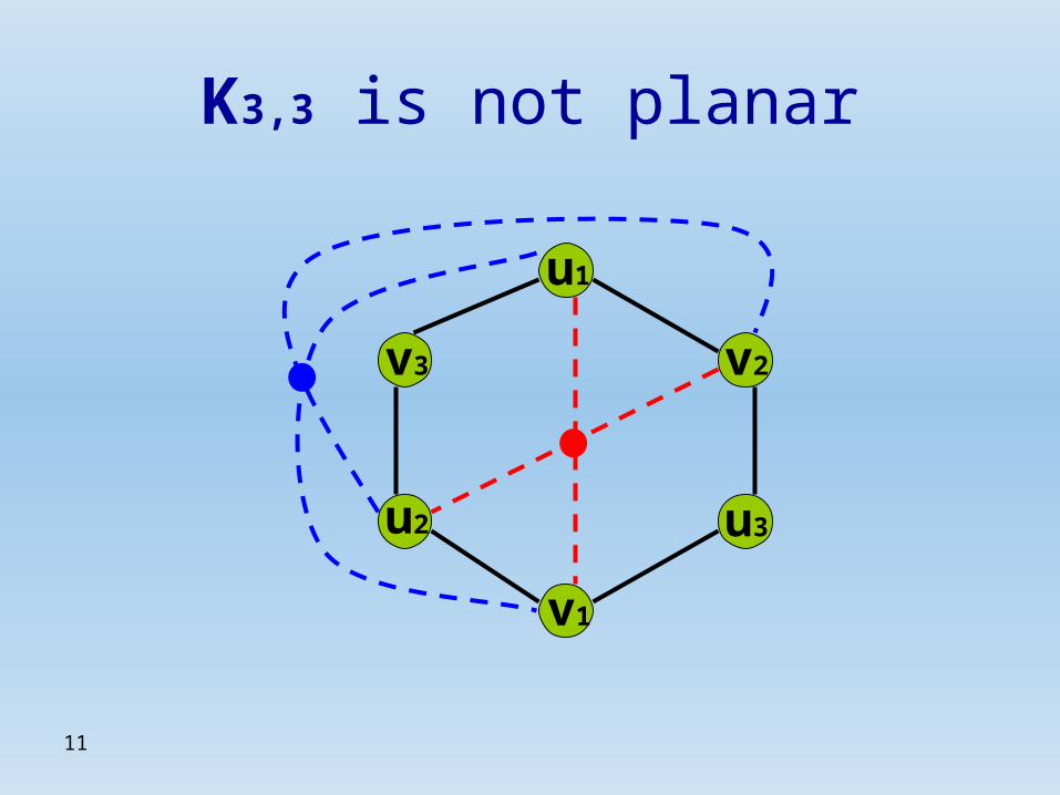
K3,3 is not planar
v3
u1
v2
u2
v1
u3
12
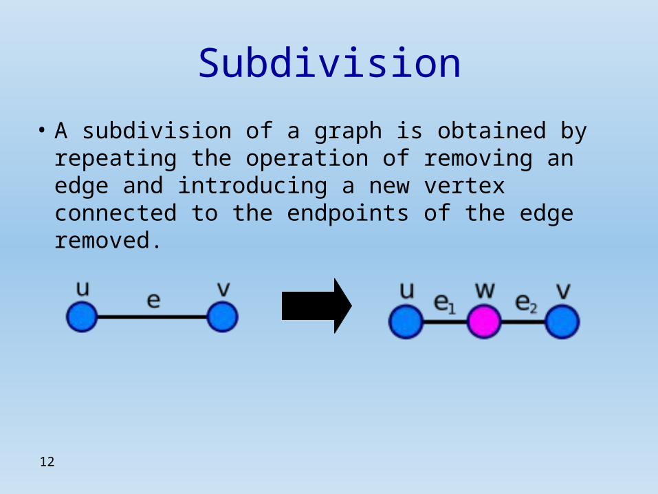
Subdivision
• A subdivision of a graph is obtained by repeating the operation of removing an edge and introducing a new vertex connected to the endpoints of the edge removed.
13
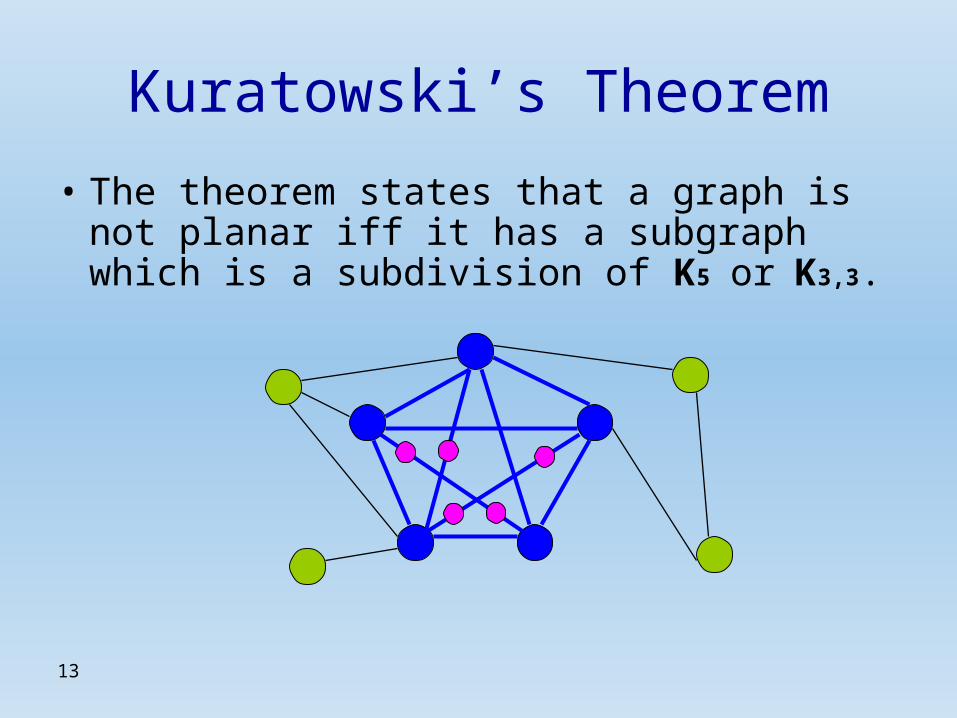
Kuratowski’s Theorem
• The theorem states that a graph is not planar iff it has a subgraph which is a subdivision of K5 or K3,3.
14
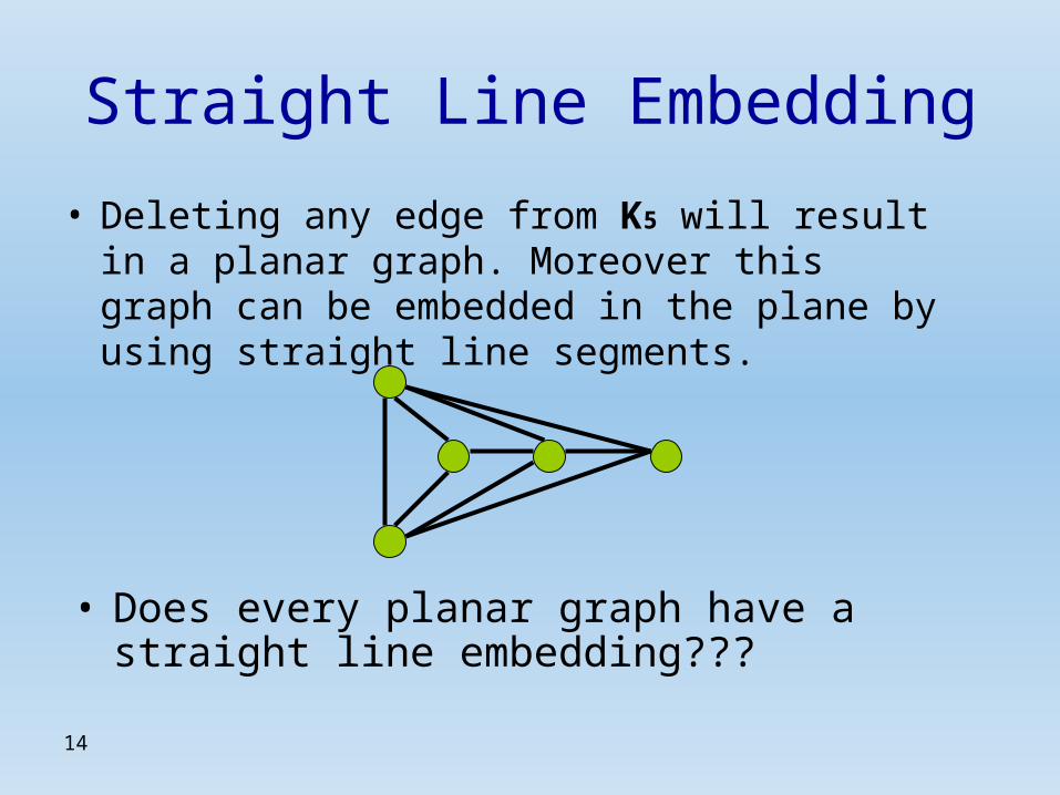
Straight Line Embedding
• Deleting any edge from K5 will result in a planar graph. Moreover this graph can be embedded in the plane by using straight line segments.
• Does every planar graph have a straight line embedding???
15
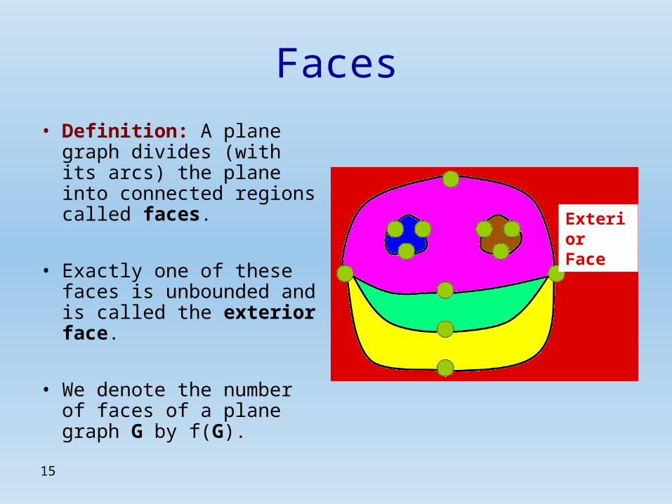
Faces
• Definition: A plane graph divides (with its arcs) the plane into connected regions called faces.
• Exactly one of these faces is unbounded and is called the exterior face.
• We denote the number of faces of a plane graph G by f(G).
Exterior Face
16
Dual Graph
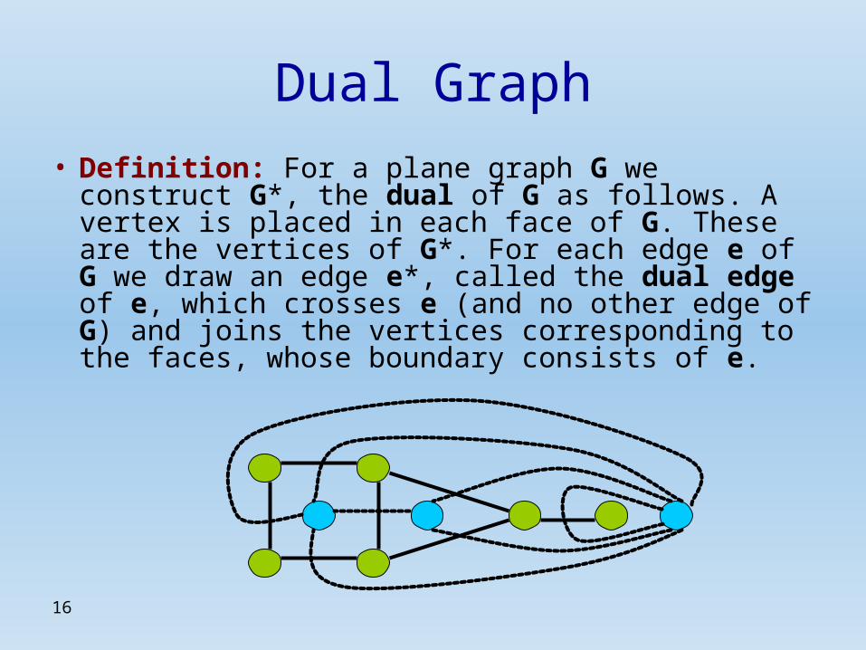
• Definition: For a plane graph G we construct G*, the dual of G as follows. A vertex is placed in each face of G. These are the vertices of G*. For each edge e of G we draw an edge e*, called the dual edge of e, which crosses e (and no other edge of G) and joins the vertices corresponding to the faces, whose boundary consists of e.

17
Euler’s Formula
• For a connected plane graph G:
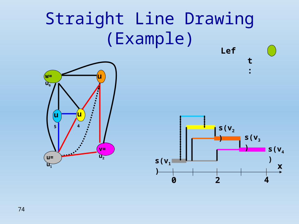
v( ) - e( ) + f( ) = 2G G G
v = 5
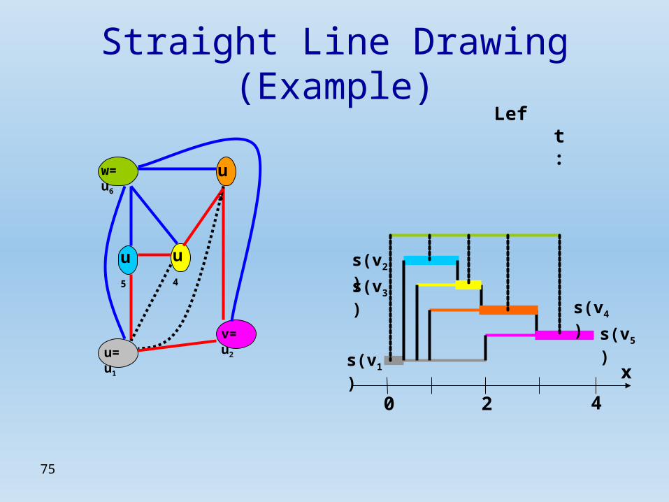
e = 7
f = 4
18
Euler’s Formula (Proof)
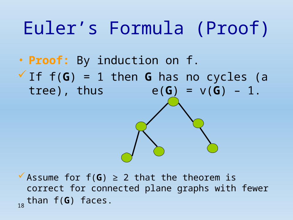
• Proof: By induction on f. If f(G) = 1 then G has no cycles (a tree), thus
e(G) = v(G) – 1.
Assume for f(G) ≥ 2 that the theorem is correct for connected plane graphs with fewer than f(G) faces.
19
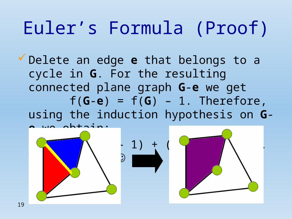
Euler’s Formula (Proof)
Delete an edge e that belongs to a cycle in G. For the resulting connected plane graph G-e we get f(G-e) = f(G) – 1. Therefore, using the induction hypothesis on G-e we obtain:
v(G) – (e(G) – 1) + (f(G) – 1) = 2. ☺
20
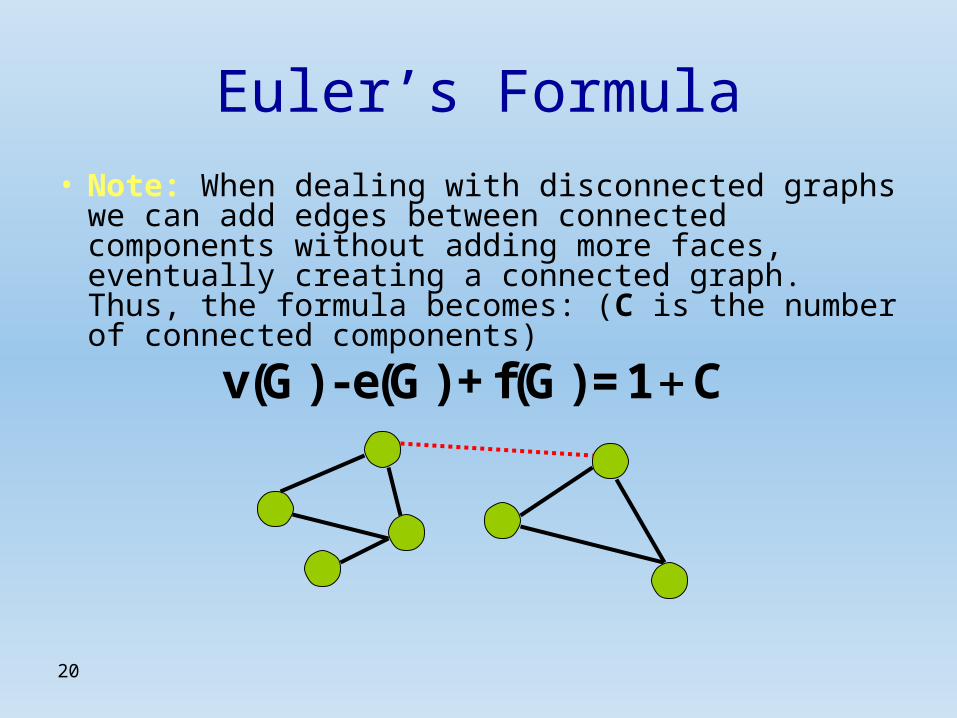
Euler’s Formula
• Note: When dealing with disconnected graphs we can add edges between connected components without adding more faces, eventually creating a connected graph. Thus, the formula becomes: (C is the number of connected components)
v(G) - e(G) + f(G) = 1 C
21
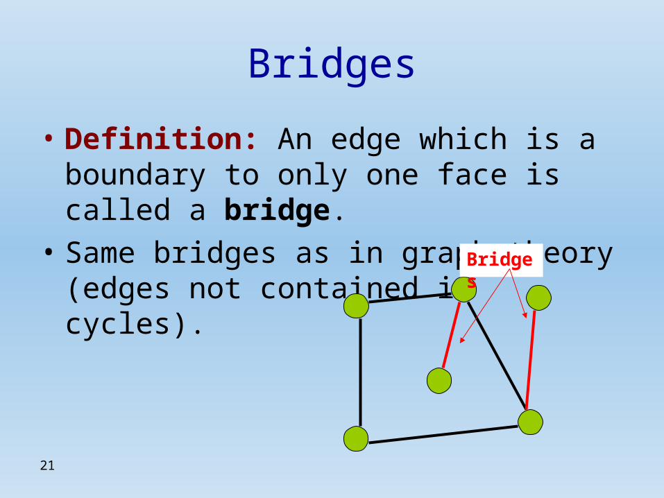
Bridges
• Definition: An edge which is a boundary to only one face is called a bridge.
• Same bridges as in graph theory (edges not contained in cycles). Bridges
22
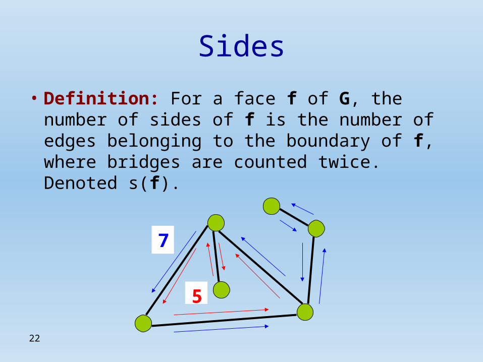
Sides
• Definition: For a face f of G, the number of sides of f is the number of edges belonging to the boundary of f, where bridges are counted twice. Denoted s(f).
5
7
23
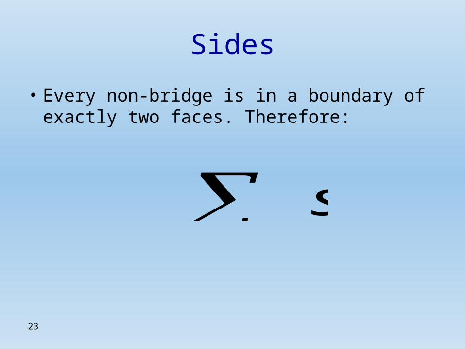
Sides
• Every non-bridge is in a boundary of exactly two faces. Therefore:
( )
( ) 2 ( )f F G
s f e G
24
Euler’s Formula
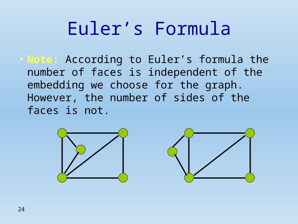
• Note: According to Euler’s formula the number of faces is independent of the embedding we choose for the graph. However, the number of sides of the faces is not.
25
Triangulation
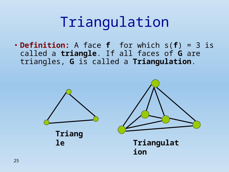
• Definition: A face f for which s(f) = 3 is called a triangle. If all faces of G are triangles, G is called a Triangulation.
TriangleTriangulation
26
Triangulation
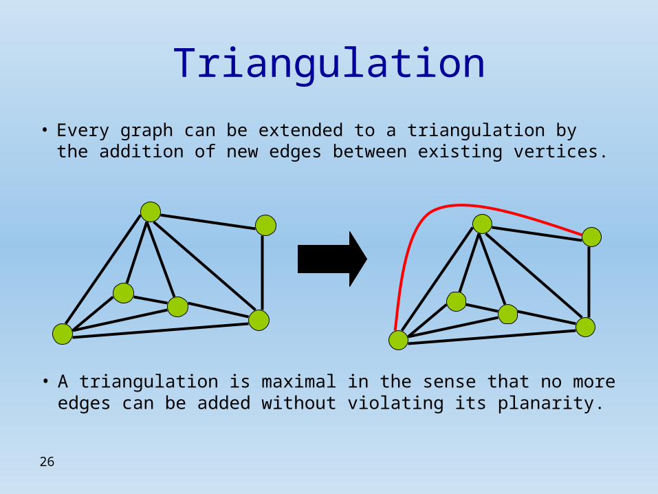
• Every graph can be extended to a triangulation by the addition of new edges between existing vertices.
• A triangulation is maximal in the sense that no more edges can be added without violating its planarity.
27
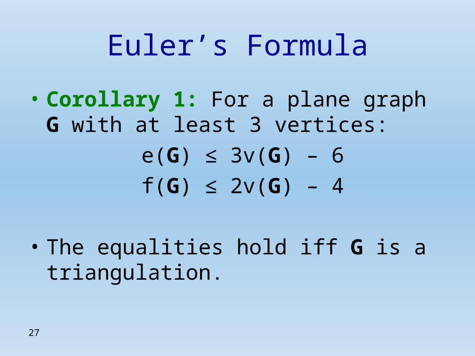
Euler’s Formula
• Corollary 1: For a plane graph G with at least 3 vertices:
e(G) ≤ 3v(G) – 6
f(G) ≤ 2v(G) – 4
• The equalities hold iff G is a triangulation.
28
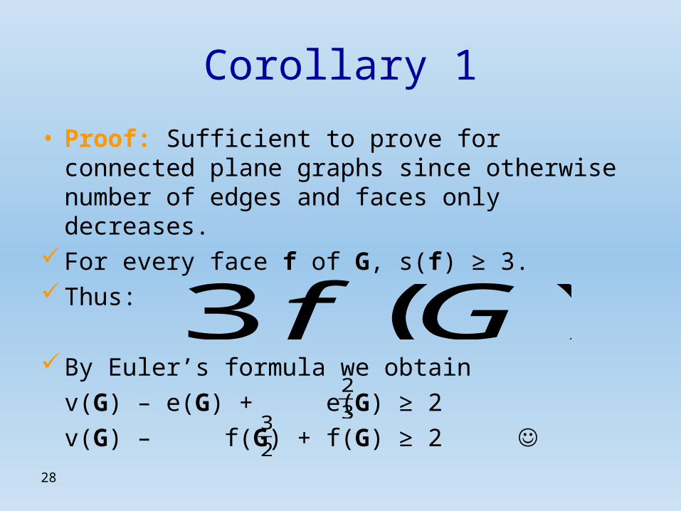
Corollary 1
• Proof: Sufficient to prove for connected plane graphs since otherwise number of edges and faces only decreases.
For every face f of G, s(f) ≥ 3.Thus:
By Euler’s formula we obtain
v(G) – e(G) + e(G) ≥ 2
v(G) – f(G) + f(G) ≥ 2 ☺
( )
3 ( ) ( ) 2 ( )f F G
f G s f e G
2
33
2
29
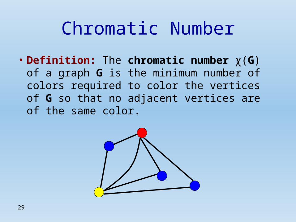
Chromatic Number
• Definition: The chromatic number χ(G) of a graph G is the minimum number of colors required to color the vertices of G so that no adjacent vertices are of the same color.
30
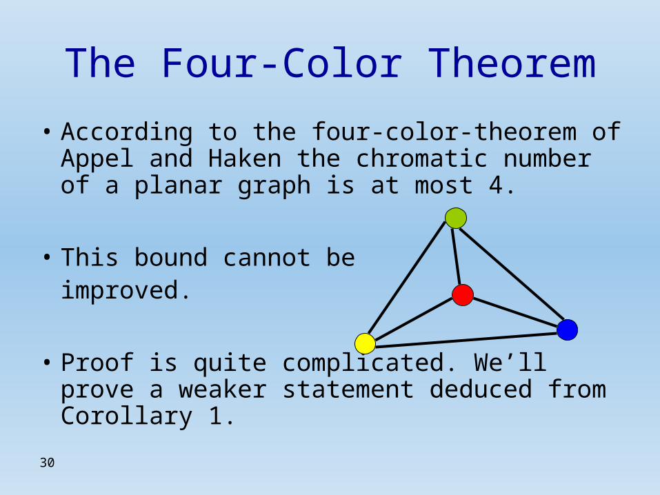
The Four-Color Theorem
• According to the four-color-theorem of Appel and Haken the chromatic number of a planar graph is at most 4.
• This bound cannot be improved.
• Proof is quite complicated. We’ll prove a weaker statement deduced from Corollary 1.
31
Corollary 2
• Corollary 2: If G is a planar graph, then χ(G) ≤ 5.• Proof: By induction on v(G). If v(G) ≤ 5, we can assign every vertex a different
color.Assume that for v(G) ≥ 6 we proved the statement for
graphs of size smaller than v(G).
32
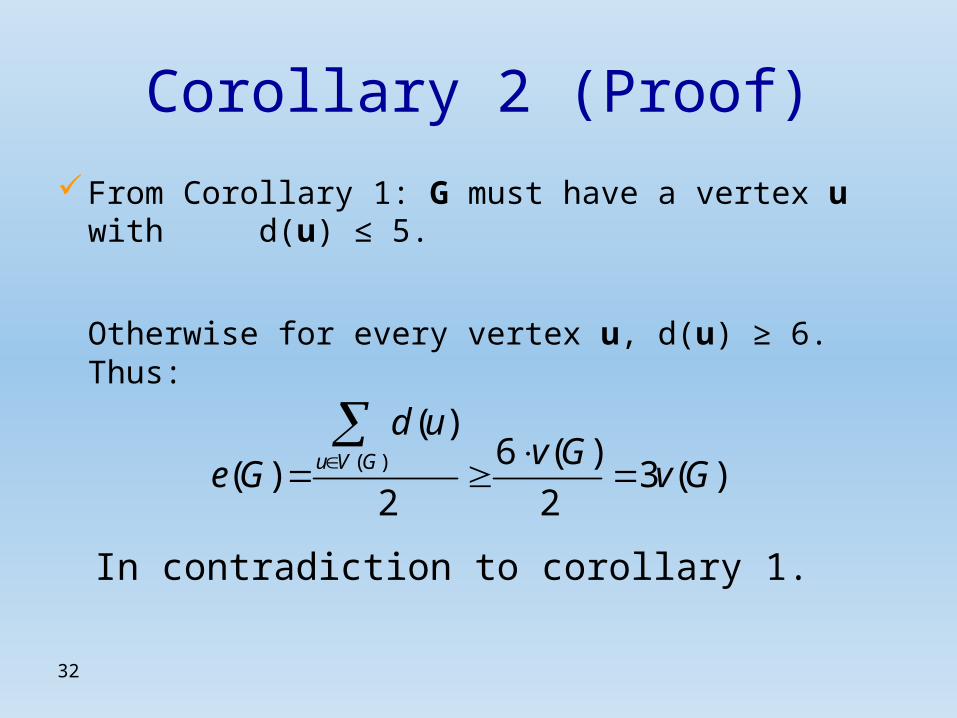
Corollary 2 (Proof)
From Corollary 1: G must have a vertex u with d(u) ≤ 5.
Otherwise for every vertex u, d(u) ≥ 6. Thus:
( )
( )6 ( )
( ) 3 ( )2 2
u V G
d uv G
e G v G
In contradiction to corollary 1.
33
Corollary 2 (Proof)
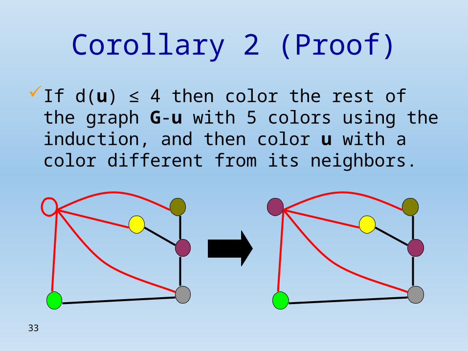
If d(u) ≤ 4 then color the rest of the graph G-u with 5 colors using the induction, and then color u with a color different from its neighbors.
34
Corollary 2 (Proof)
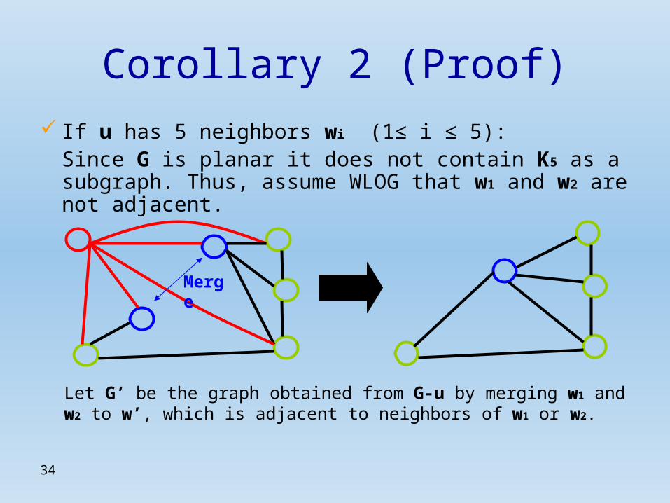
If u has 5 neighbors wi (1≤ i ≤ 5):Since G is planar it does not contain K5 as a subgraph. Thus, assume WLOG that w1 and w2 are not adjacent.
Let G’ be the graph obtained from G-u by merging w1 and w2 to w’, which is adjacent to neighbors of w1 or w2.
Merge
35
Corollary 2 (Proof)
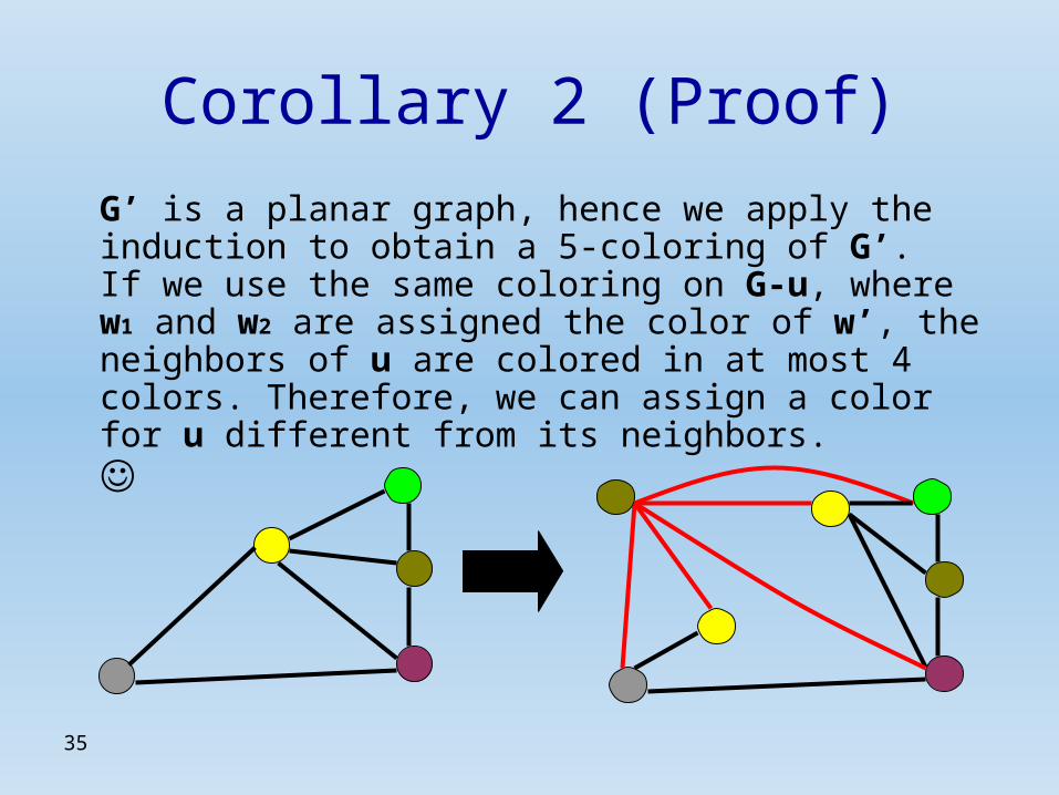
G’ is a planar graph, hence we apply the induction to obtain a 5-coloring of G’. If we use the same coloring on G-u, where w1 and w2 are assigned the color of w’, the neighbors of u are colored in at most 4 colors. Therefore, we can assign a color for u different from its neighbors. ☺
36
Straight Line Drawing
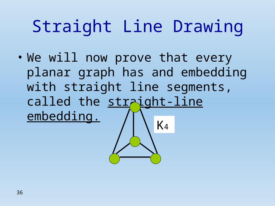
• We will now prove that every planar graph has and embedding with straight line segments, called the straight-line embedding.
K4
37
u1
Straight Line Drawing
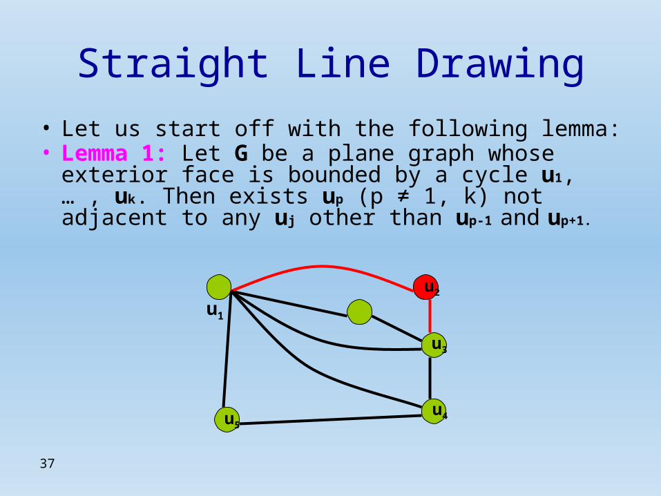
• Let us start off with the following lemma:• Lemma 1: Let G be a plane graph whose exterior
face is bounded by a cycle u1, … , uk. Then exists up (p ≠ 1, k) not adjacent to any uj other than up-1 and
up+1.
u2
u3
u4 u5

38
u1
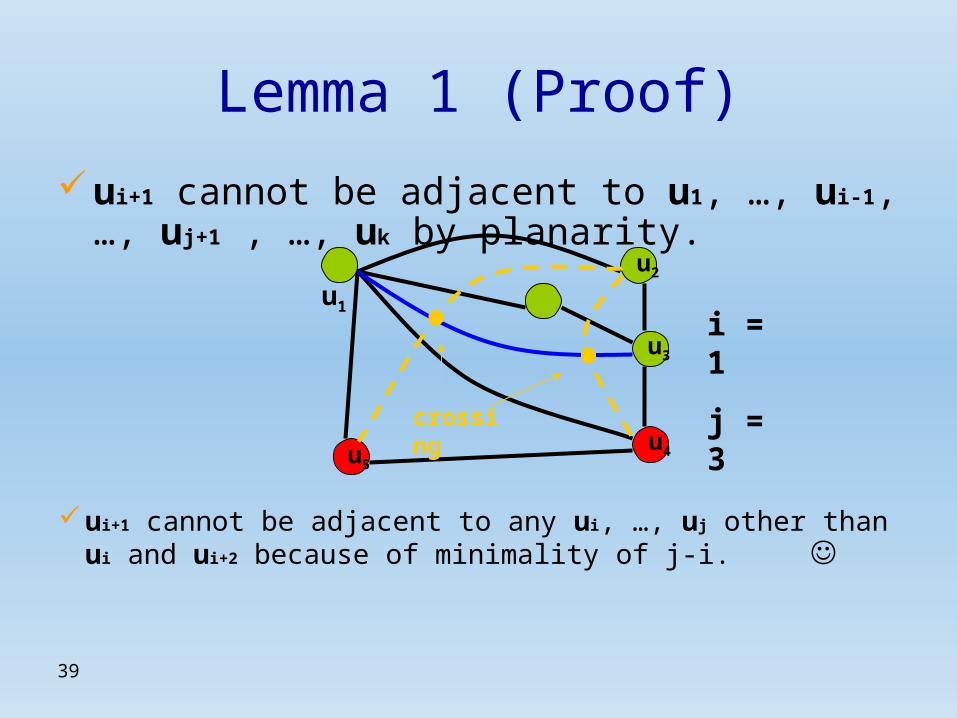
Lemma 1 (Proof)
• Proof: If no two non-consecutive vertices in the exterior boundary are adjacent, then the lemma is trivial. Otherwise:
Pick two non-consecutive adjacent vertices ui, uj (j > i+1) for which j-i is minimal.
u2
u3
u4 u5
i = 1
j = 3
39
u1
Lemma 1 (Proof)
ui+1 cannot be adjacent to u1, …, ui-1, …, uj+1 , …, uk by planarity.
u2
u3
u4 u5
crossing
ui+1 cannot be adjacent to any ui, …, uj other than ui and ui+2 because of minimality of j-i. ☺
i = 1
j = 3
40
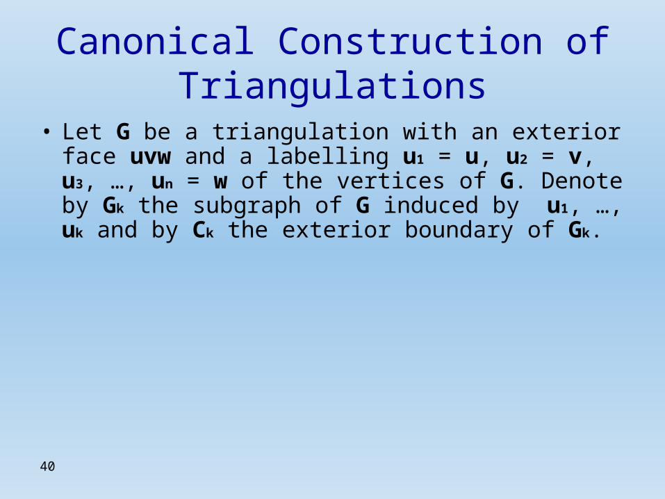
Canonical Construction of Triangulations
• Let G be a triangulation with an exterior face uvw and a labelling u1 = u, u2 = v, u3, …, un = w of the vertices of G. Denote by Gk the subgraph of G induced by u1, …, uk and by Ck the exterior boundary of Gk.

41
Canonical Construction of Triangulations
• There exists a labelling such that for every 4 ≤ k ≤ n:
I. Gk-1 is internally triangulated.
II. The edge uv is in Ck-1.
III. uk is in the exterior face of Gk-1 the neighbors of uk in V(Gk-1) are consecutive on Ck-1.
• This kind of labelling is called a canonical labelling.
42
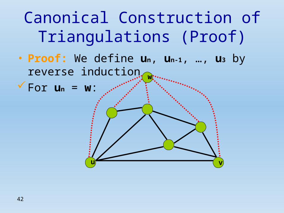
Canonical Construction of Triangulations (Proof)
• Proof: We define un, un-1, …, u3 by reverse induction.For un = w:
u v
w

43
Canonical Construction of Triangulations (Proof)
For 4 ≤ k ≤ n: Assume we defined un, …, uk correctly. Applying Lemma 1 to Gk-1, the subgraph induced by the remaining vertices, we know that there is a vertex on Ck-1, other than u and v, that is only adjacent to its preceding and subsequent vertices on Ck-1. Let uk-1 be that vertex. Proof of I.-III. is the same as with un.
☺
44
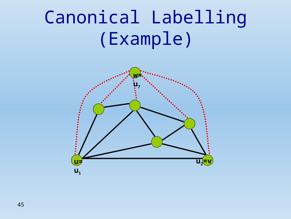
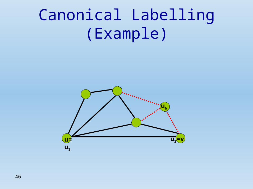
Canonical Labelling (Example)
u v
w
45
Canonical Labelling (Example)
u= u1u2=v
w= u7
46
Canonical Labelling (Example)
u= u1u2=v
u6

47
Canonical Labelling (Example)
u= u1u2=v
u5
48
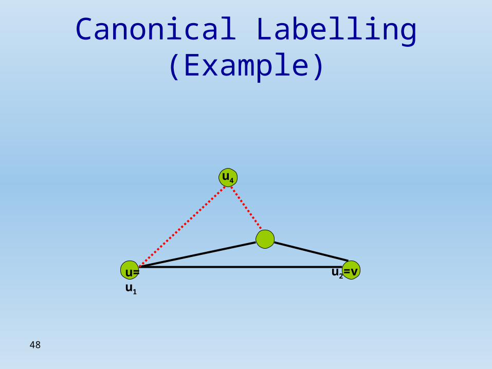
Canonical Labelling (Example)
u= u1u2=v
u4
49
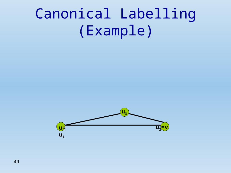
Canonical Labelling (Example)
u= u1u2=v
u3
50
Straight Line Drawing
• Corollary 3: Every planar graph has a straight line embedding in the plane.
• Proof: It is sufficient to show that the statement is true for any maximal planar graph, i.e. a graph that can be represented as a triangulation.

51
Corollary 3 (Proof)
Let G be a triangulation with the canonical labelling u1 = u, u2 = v, u3, …, un = w as described earlier. We will determine the positions p(uk) = (x(uk), y(uk)) of the vertices by induction on k.
52
Corollary 3 (Proof)
Set p(u1) = (0,0) , p(u2) = (2,0) , p(u3) = (1,1).
For k ≥ 4 assume that p(u1), …, p(uk-1) have already been defined s.t., by connecting the images of adjacent vertices with segments, we obtain a straight line embedding of Gk-1, whose exterior face is bounded by the segments corresponding to the edges of Ck-1.

53
Corollary 3 (Proof)
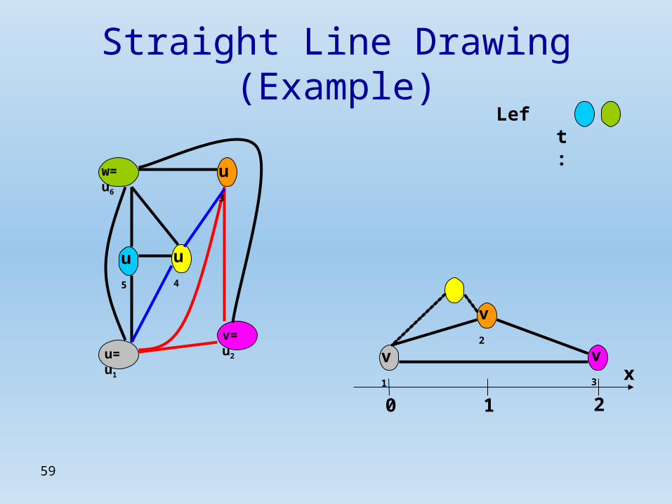
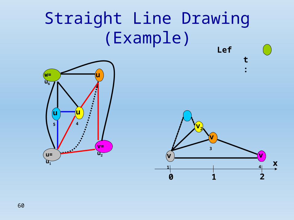
Let v1 = u, v2, …, vm = v denote the vertices of Ck-1 listed in the order they appear on the cycle.Suppose further that:
(1) x(v1) < x(v2) < … < x(vm)y(vi) > 0 for 1 < i < m
54
Corollary 3 (Proof)
By condition III. of the canonical labelling, uk is connected to a series of consecutive vertices of Ck-1, vq, …, vr (1 ≤ q < r ≤ m). Choose x(uk) s.t. x(vq) < x(uk) < x(vr). Now choose y(uk) > 0 large enough. The new position p(uk) meets all the requirements (including the assumption (1)). ☺
55
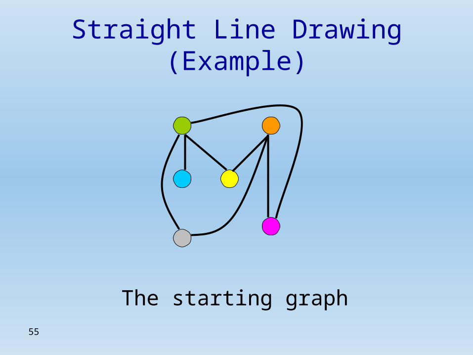
Straight Line Drawing (Example)
The starting graph

56
Straight Line Drawing (Example)
Making the triangulation
57
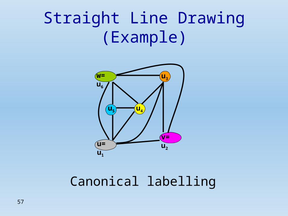
Straight Line Drawing (Example)
u= u1
v= u2
w= u6
u5 u4
u3
Canonical labelling

58
Straight Line Drawing (Example)
u= u1
v= u2
w= u6
u5u4
u3
Left:
0 1 2
x
Setting p(u1) p(u2) p(u3)
59
Straight Line Drawing (Example)
u= u1
v= u2
w= u6
u5u4
u3
Left:
0 1 2
xv1
v2
v3
60
Straight Line Drawing (Example)
u= u1
v= u2
w= u6
u5u4
u3
Left:
0 1 2
xv1
v3
v4
v2

61
Straight Line Drawing (Example)
u= u1
v= u2
w= u6
u5u4
u3
Left:
0 1 2
xv1
v3
v4
v2
v5
62
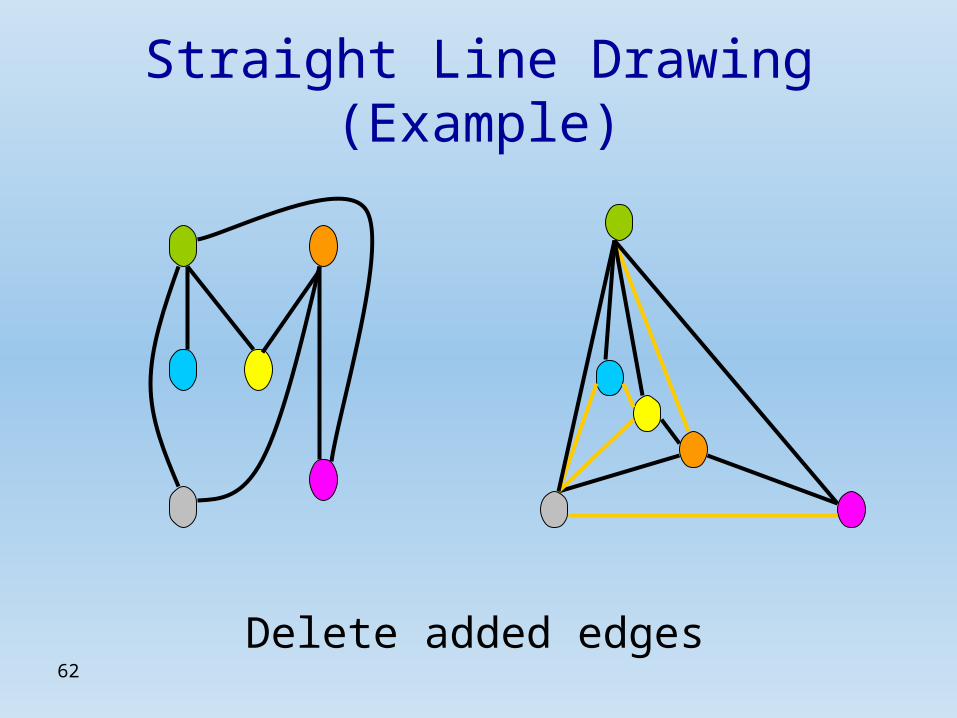
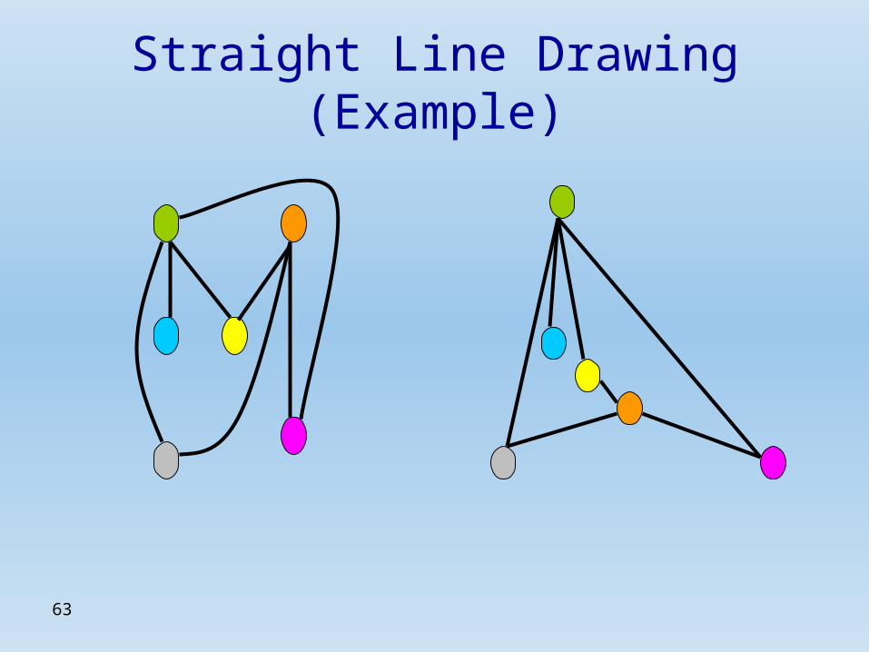
Straight Line Drawing (Example)
Delete added edges
63
Straight Line Drawing (Example)
64
Straight Line Drawing
• Note: By using this method we can also establish the existence of straight line embedding of other representations. For example, straight line embeddings of the following representation, found by Rosenstiehl and Tarjan.
65
Straight Line Drawing
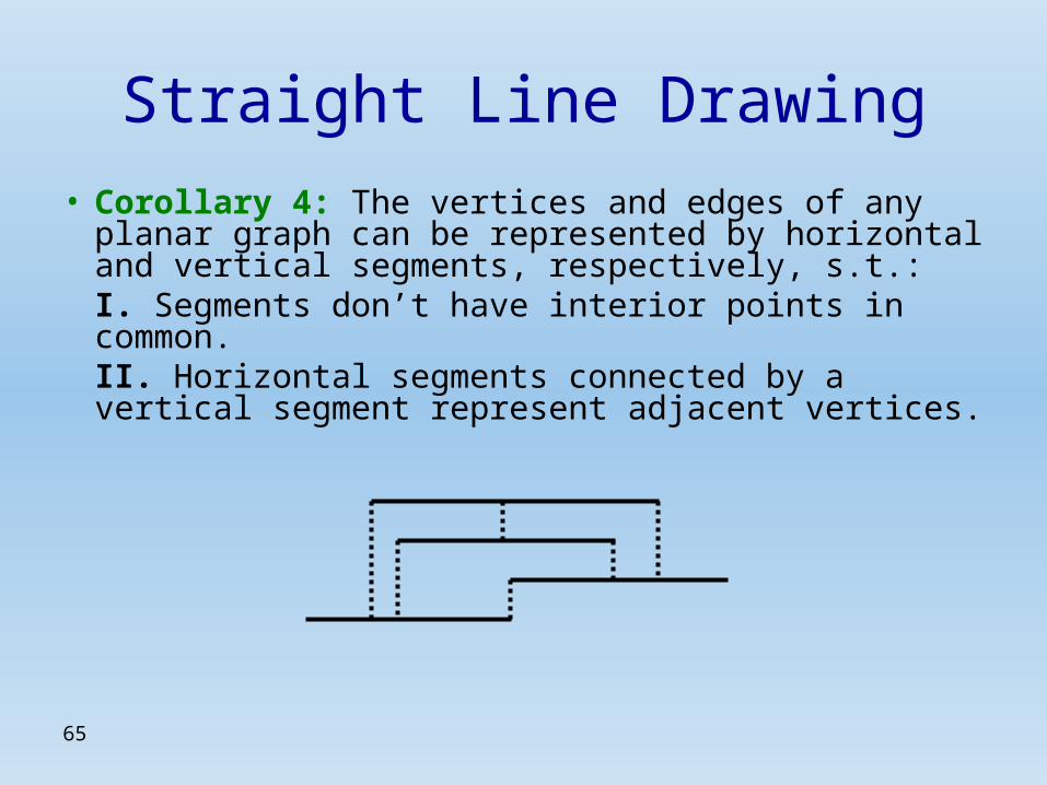
• Corollary 4: The vertices and edges of any planar graph can be represented by horizontal and vertical segments, respectively, s.t.:I. Segments don’t have interior points in common.II. Horizontal segments connected by a vertical segment represent adjacent vertices.

66
Corollary 4 (Proof)
• Proof: As earlier it is sufficient to establish the statement for triangulations.
Let G be a triangulation with the canonical labelling u1 = u, u2 = v, u3, …, un = w. To every uk we will assign a segment s(uk) whose endpoints are (xk, k) and (x'k, k).
67
Corollary 4 (Proof)
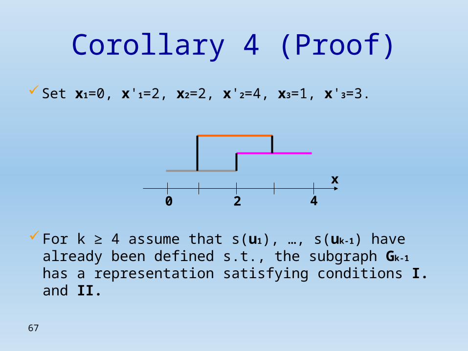
Set x1=0, x'1=2, x2=2, x'2=4, x3=1, x'3=3.
For k ≥ 4 assume that s(u1), …, s(uk-1) have already been defined s.t., the subgraph Gk-1 has a representation satisfying conditions I. and II.
0 2 4
x
68
Corollary 4 (Proof)
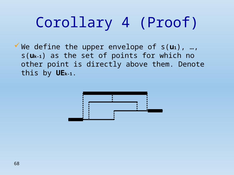
We define the upper envelope of s(u1), …, s(uk-1) as the set of points for which no other point is directly above them. Denote this by UEk-1.
69
Corollary 4 (Proof)
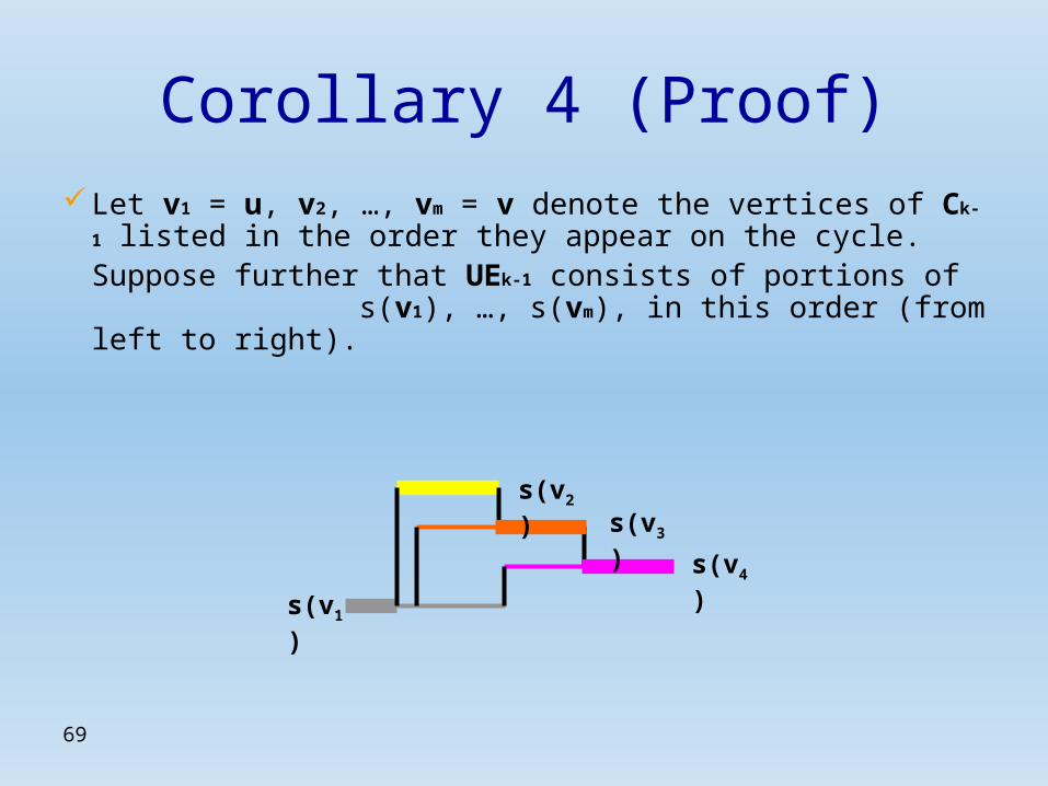
Let v1 = u, v2, …, vm = v denote the vertices of Ck-1 listed in the order they appear on the cycle.Suppose further that UEk-1 consists of portions of s(v1), …, s(vm), in this order (from left to right).
s(v1)
s(v3)s(v2)
s(v4)
70
Corollary 4 (Proof)
By condition III. of the canonical labelling, uk is connected to a series of consecutive vertices of Ck-1, vq, …, vr (1 ≤ q < r ≤ m). Choose xk to be some point of s(vq) which belongs to UEk-1 and choose x'k to be some point which belongs to UEk-1. The resulting representation of Gk meets the requirements. ☺

71
Straight Line Drawing (Example)
u= u1
v= u2
w= u6
u5 u4
u3
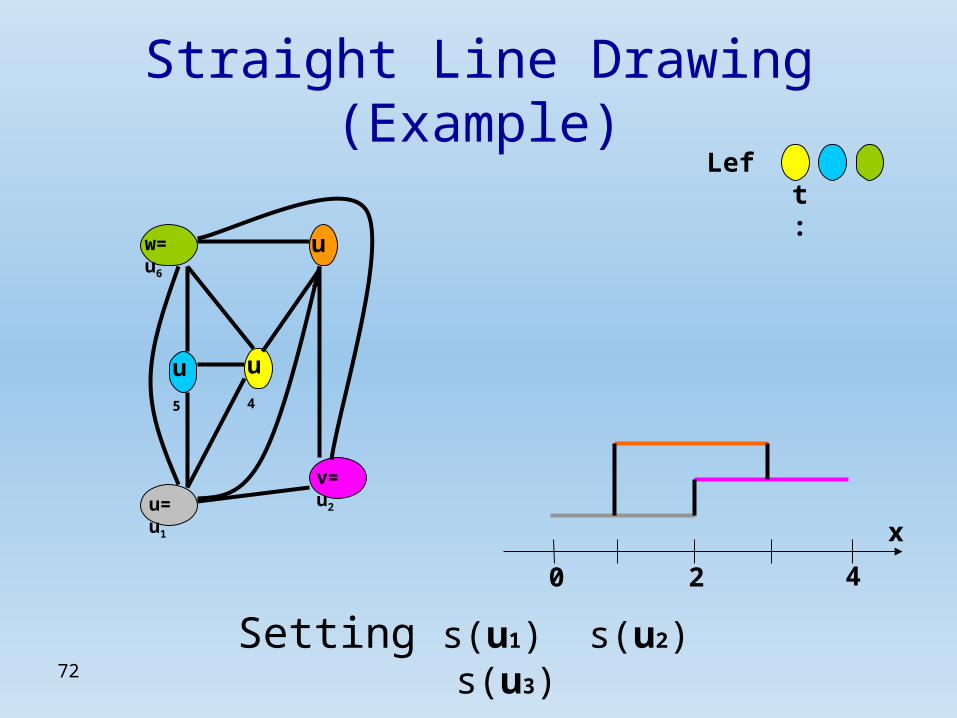
Canonical labelling
72
Straight Line Drawing (Example)
u= u1
v= u2
w= u6
u5u4
u3
Left:
0 2 4
x
Setting s(u1) s(u2) s(u3)
73
Straight Line Drawing (Example)
u= u1
v= u2
w= u6
u5u4
u3
Left:
0 2 4
xs(v1)
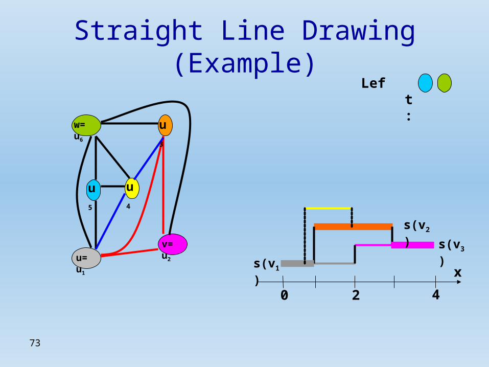
s(v3)
s(v2)
74
Straight Line Drawing (Example)
u= u1
v= u2
w= u6
u5u4
u3
Left:
0 2 4
xs(v1)
s(v3)s(v2)
s(v4)
75
Straight Line Drawing (Example)
u= u1
v= u2
w= u6
u5u4
u3
Left:
0 2 4
xs(v1)
s(v3)
s(v2)
s(v4)
s(v5)
76
Straight Line Drawing (Example)
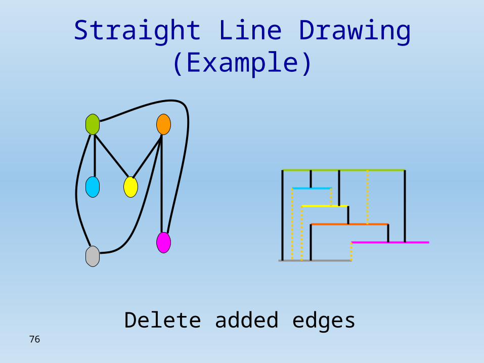
Delete added edges
77
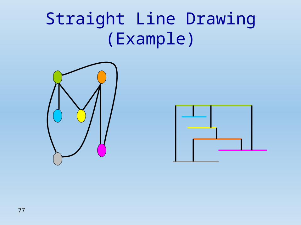
Straight Line Drawing (Example)

78
3D Implementations
• So far we’ve seen embeddings of graphs in 2D (on the plane).
• We will now see how to embed planar graphs in 3D.
• We will also get to know new shapes which allow use to draw graphs which are not planar.

79
The Sphere
• Every planar graph can be embedded on the sphere.
• Likewise, every embedding on the sphere can be transformed to an embedding on the plane.
80
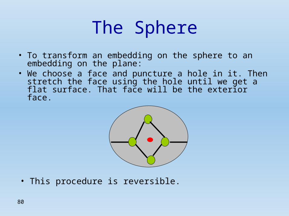
The Sphere
• To transform an embedding on the sphere to an embedding on the plane:
• We choose a face and puncture a hole in it. Then stretch the face using the hole until we get a flat surface. That face will be the exterior face.
• This procedure is reversible.
81
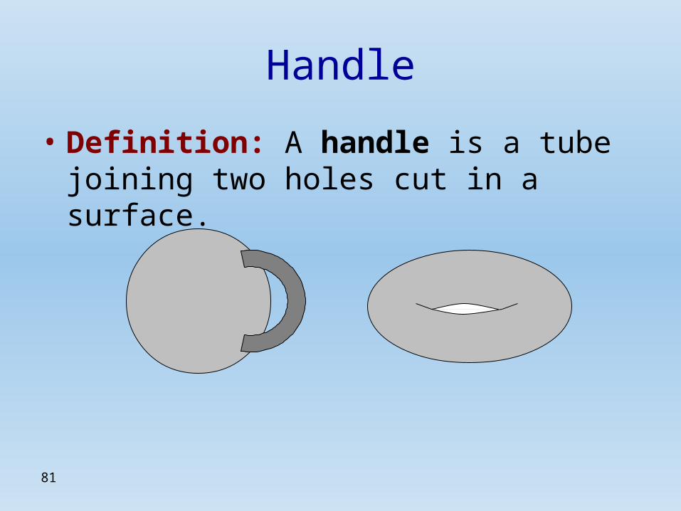
Handle
• Definition: A handle is a tube joining two holes cut in a surface.
82
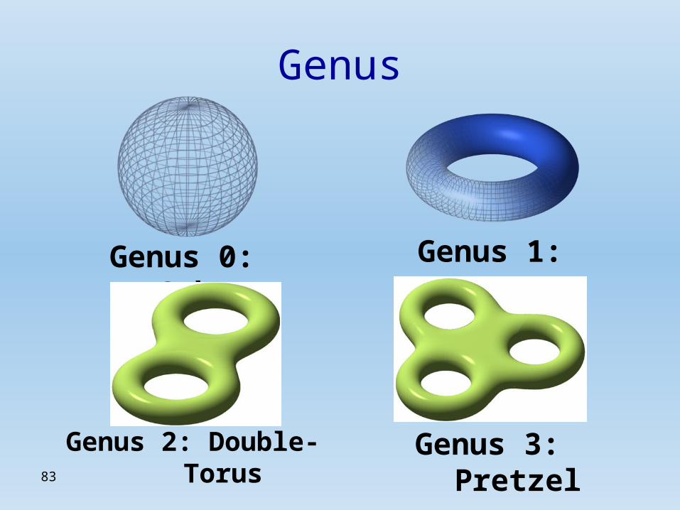
Genus
• Definition: The genus of a surface obtained by adding handles to a sphere is the number of spheres added.
83
Genus
Genus 0: Sphere Genus 1: Torus
Genus 2: Double-Torus Genus 3: Pretzel
84
Graphs
• The genus of a graph is the minimum γ such that the graph can be embedded on a surface of genus γ.
• As stated planar graphs can be embedded on the sphere. Therefore, they are of genus 0.
85
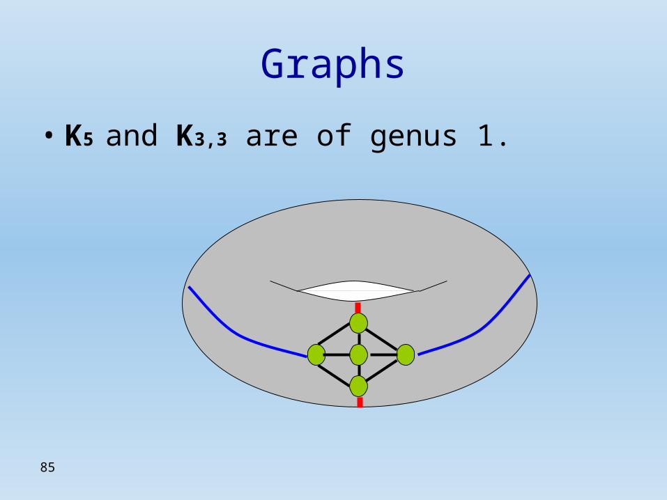
Graphs
• K5 and K3,3 are of genus 1.