Computational Fluid Dynamics (CFD) Analysis of Air Based Building Integrated Photovoltaic Thermal (BIPV/T) Systems for

Efficient Performance

H. Getu1,* T. Yang2, A. K. Athienitis2, A. Fung1,

1Department of Mechanical and Industrial Engineering, Ryerson University, 350 Victoria Street, Toronto, ON, Canada M5B 2K3

2Dept. of Building, Civil and Environmental Engineering, Concordia University, 1515 St. Catherine W., Montréal, Québec, Canada

*corresponding author: ghailu@ryerson.ca, Tel. 1-416-979-5000, x 4097, FAX. 1-416-979-5265

Abstract

This paper presents CFD study of BIPV/T systems with forced convection using air as a coolant with various air flow rates (air velocities). Predictions of the PV’s back surface, the air inside the channel and the insulation temperature profiles were compared with experimentally obtained temperature profiles. COMSOL Multiphysics finite element analysis (FEA) software was used to develop CFD models for a BIPV/T system; and to investigate the accuracy of predictions of temperature profiles using the k-ε and k-ω turbulence models. Turbulent flows were considered with Reynolds number ranging from 2577 to 9392. Predictions of the PV’s back surface temperature, the temperature of the flowing air and the insulation temperature agreed very well with the measured temperatures. The results indicate that CFD could be used to obtain temperature profiles in order to establish relationships between the average/local convective heat transfer coefficients and air flow velocity. The relationships obtained will be useful for simple mathematical models that facilitate the design and optimization of different parts of the BIPV/T system.

1 Introduction Solar energy is inexhaustible and import-independent resource that enhances energy security

and sustainability, reduces pollution, lowers the cost of mitigating climate change, and keeps fossil fuel prices lower than otherwise (Solar Energy Perspectives, 2011). Photovoltaic panels with a heat recovery capability, integrated into the building envelope replacing the elements of the roof or façade combine the possibility of cooling the PV panels, producing electricity and heat (Pantic et al., 2010). Building integrated photovoltaic (BIPV/T) systems are arrays of photovoltaic panels integrated into the building structures as facades and roofs that can produce electricity and useful thermal energy (Pantic et al., 2010; Chen et al., 2007; Chen et al., 2010a; Chen et al., 2010b; Candanedo and Athienitis 2008; Dembo et al., 2010). Heat recovery would be accomplished by fluid circulation behind the array of photovoltaic modules, which heat up when exposed to sunlight. The heat recovered by fluid circulation behind the photovoltaic panels can be used for space and/or domestic water heating. BIPV/T systems have the potential to meet all the building envelope requirements such as mechanical resistance and thermal insulation. In addition to producing heat and electricity, the multiple functionality of BIPV/T system may improve the cost effectiveness of residential construction as compared to add-on PV/T systems. Various researchers have studied integration of PV panels into building structures such as roofs and façades with a focus not only on the design of BIPV/T system themselves and evaluation of their energy performance (Chen et al., 2010a; Chen et al., 2010b; Candanedo and Athienitis, 2008; Dembo et al., 2010; Safa, 2012; Candanedo et al., 2010; Mei et al., 2003; Infield et al., 2004, 2006; Cartmell et al., 2004; Chow et al., 2007; Charron, and Athienitis, 2006; Getu et al., 2013; Getu and Fung 2014).

For optimal electricity production and thermal energy recovery it is important to study the fluid flow behaviour in the air channel of an integrated photovoltaic/thermal panels in order to obtain detailed information on air velocity and temperature distributions, and determination of convective heat transfer coefficients as a function of air velocity and air flow channel size. In order to obtain reliable data it is important to address the coupled fluid flow and heat transfer problem of the BIPV/T system. It is often difficult, if not impossible, to obtain closed form solutions to the governing heat transfer and fluid mechanics equations through theoretical calculations. Furthermore, in most cases, the obtained solutions contain infinite series and transcendental equations, making their numerical evaluation a difficult task (Patankar, 1980). Full scale experimental investigations are costly and some variables such as heat transfer coefficients are impossible to measure directly. Computational fluid dynamics (CFD) can be used to obtain relationships between the average and local convective heat transfer coefficients, velocity and channel depth.

Liao et al. (2007) conducted a CFD study of heat transfer and fluid flow in a facade-integrated photovoltaic-thermal system intended for single story application. They found that the convective heat transfer coefficients to be generally higher than the predictions reported in literature (Charron and Athienitis, 2006). They attributed this to the leading-edge effects and the turbulent nature of the flow. The effects of flow rate and configuration in PV/T systems on the overall system performance were studied using CFD simulation (Naewngerndee et al., 2011). They found that for the same number of PV/T modules (16), a 4x4 configuration provided better flow distribution, when compared to an 8x2 configuration. When the total number of PV/T modules was reduced to 12, they found that a 3x4 configuration resulted in the most suitable flow distribution, as compared to the 4x3 and 6x2 configurations. Gan and Riffat used FLUENT to analyze air flow condition and temperature distribution in an atrium integrated with photovoltaics

(Gan and Riffat, 2004). They found that for effective cooling of the roof integrated PV arrays, outdoor air should be introduced through an opening positioned close to the roof or through an air channel underneath the roof. Corbin and Zhai conducted an experimentally validated CFD study to determine the effect of active heat recovery by circulating water on the performance of PV panels (Corbin and Zhai, 2010). Their parametric analysis showed that the PV efficiency increased by 5.3% and that the water temperature was suitable for domestic use. A CFD study of an open loop BIPV/T system was conducted in order to obtain convective heat transfer coefficients under different mass flow rates and design conditions (Candanedo et al., 2008 and 2009). They found that the optimum airflow rate depended on the channel geometry and the required outlet air temperature. From this brief review it is clear that CFD can be used to obtain information related to flow dynamics, which is useful for establishing correlations that can be applied in the design optimization of BIPV/T systems.

In this work, COMSOL Multiphysics FEA software was used to develop CFD models for an open loop BIPV/T system. The aim is to compare predictions of PV’s backside, flowing air and insulation temperature profiles with experimentally obtained profiles. This is done using two commonly used turbulence models (k-ε and k-ω) with various air flow rates (air velocities).

2 CFD Simulation COMSOL CFD program was used to simulate the fluid and heat transfer phenomena for the

BIPV/T configuration. The COMSOL CFD package was selected because it integrates the preprocessor (geometry and mesh generation) and the solver, whereas other packages such as Fluent (a solver) require a preprocessor such as GAMBIT. Perhaps, the most important advantage of COMSOL is that it provides multiphysics environment which facilitates solutions to coupled physics problems such as fluid flow and heat transfer problems. In this work, a 2D model was created that represents the geometry of the studied BIPV/T system.

Turbulence modeling The COMSOL CFD module uses Reynolds Averaged Navier-Stokes (RANS) models which

divide the flow quantities into an averaged value and fluctuating part (COMSOL 4.3b). Once the flow has become turbulent, all quantities fluctuate in time and space. It is extremely computationally costly to obtain detailed information about the fluctuations. An averaged representation often provides sufficient information about the flow (COMSOL 4.3b).

For the simulations, standard k-ε and k-ω turbulence models were used. The Non-Isothermal Flow and Conjugate Heat Transfer were used in COMSOL. This module includes the Non-Isothermal Flow predefined multiphysics coupling to simulate systems where density varies with temperature. The formulation of the continuity and momentum equations for this physics are as follows. ( )u 0∇ ⋅ ρ = (1)

( ) ( ) ( )( ) ( )( )TT T

2 2u u pI u u u I kI F3 3

ρ ⋅∇ = ∇ ⋅ − + µ + µ ∇ + ∇ − µ + µ ∇ ⋅ − ρ + (2)

where ρ is the density (kg/m3) u is the velocity vector (m/s) p is the pressure (Pa)

µ is the dynamic viscosity (Pas) F is the body force vector (N/m3) I is the unit tensor where µ depends only on the physical properties of the fluid, while µT is the turbulent eddy viscosity which emulates the effect of unresolved velocity fluctuations u′. For the standard k - ε model µT is given by Eq. 9. The heat equation is

( )pTC T Qt

∂ρ = ∇ ⋅ κ∇ +

∂ (3)

where Cp is the heat capacity, κ is the thermal conductivity and Q is the heat source.

The k-ω turbulence model The k-ω model solves for the turbulent kinetic energy, k, and for the dissipation per unit

turbulent kinetic energy, ω, also commonly known as the specific dissipation rate. The CFD Module has the Wilcox revised k-ω model (Wilcox, 1998).

( ) ( )T k k 0u k k P k∗ ∗ ρ ⋅∇ = ∇ ⋅ µ + µ σ ∇ + − ρβ ϖ (4)

( ) ( ) 2

T k 0u Pkϖ

ϖρ ⋅∇ ϖ = ∇ ⋅ µ + µ σ ∇ϖ + α − ρβ ϖ (5)

where

Tk

µ = ρϖ

, 1325

α = , 0fββ = β , 0f∗ ∗

ββ = β , (6)

12

σ = , 12

∗σ = , 013

125β = ,

1 70f1 80

ϖβ

ϖ

+ χ=

+ χ ,

( )ij jk ki

3

0

Sϖ ∗

Ω Ωχ =

β ϖ (7)

where in turn ijΩ is the mean rotation rate tensor, i jij

j i

1 u u2 x x

∂ ∂Ω = − ∂ ∂

and ijS is the mean strain

rate tensor i jij

j i

1 u uS2 x x

∂ ∂= + ∂ ∂

where the production term, Pk is

( )( ) ( )T 2k T

2 2P u : u u u k u3 3

= µ ∇ ∇ + ∇ − ∇ ⋅ − ρ ∇ ⋅ (8)

Note that the colon symbol designates matrix contraction.

The k-ε turbulence model Eq. 2 is to be complemented by two additional convection-diffusion-reaction equations for

computation of k and ε (Eq. 8 and Eq. 11). The k-ε model is one of the most used turbulence models for industrial applications. The standard k-ε model introduces two transport equations and two dependent variables: the turbulent kinetic energy, k, and the dissipation rate of turbulence energy, ε. Turbulent viscosity, µT, in is modeled by

2

TkCµµ = ρε

(9)

where Cµ is a model constant. The transport equation for k is given by:

( ) Tk

k

u k k P µ

ρ ⋅∇ = ∇ ⋅ µ + ∇ + − ρε σ . (10)

where the production term, Pk is given by Eq. 8. The transport equation for ε is given by:

( )2

T1 k 2u C P C

k kε εε

µ ε ερ ⋅∇ ε = ∇ ⋅ µ + ∇ε + − ρ σ

. (11)

The model constants in Eq. 9, Eq. 10 and Eq. 11 are determined from experimental data (Wilcox, 1998) and the values are: Cµ =0.09, Cε1=1.44, Cε2=1.92, σk=1.0, σε=1.3

Radiation modeling COMSOL provides two radiation models: hemicube and direct area integration methods.

Hemicube is the default method and uses projections to account for shadowing effects. This method is suitable for complicated shapes which may have shadowing effect. On the other hand, with direct area integration method COMSOL evaluates the mutual irradiation between surfaces directly, without considering which face elements are obstructed by others. Direct area integration method is fast and accurate for simple geometries with no shadowing. Since the geometry of the BIPV/T system considered in this work is simple with no shadowing effect, the direct area integration method was employed.

Meshing Solving for fluid flow problem is computationally intensive. Usually, relatively fine meshes

are required. The aim was to use as simple a mesh as possible, while still capturing all of the details of the flow. A physics-controlled meshing was used in this work. A physics-controlled meshing uses sequences that examine the physics to automatically determine size attributes to the problem. For the flow problem solved in this work, the velocity field changes quite slowly in the direction tangential to the wall, but rapidly in the normal direction (Fig. 1). This situation motivated the use of a boundary layer mesh. Boundary layer meshes (which are the default mesh type on walls when using physics-based meshing) insert thin rectangles in 2D near the walls. These high aspect ratio elements (Fig. 1) are suitable of resolving the variations in the flow velocity normal to the boundary, while reducing the number of calculation points in the direction tangential to the boundary (COMSOL 4.3b).

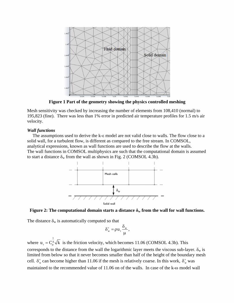
Figure 1 Part of the geometry showing the physics controlled meshing

Mesh sensitivity was checked by increasing the number of elements from 108,410 (normal) to 195,823 (fine). There was less than 1% error in predicted air temperature profiles for 1.5 m/s air velocity.

Wall functions The assumptions used to derive the k-ε model are not valid close to walls. The flow close to a

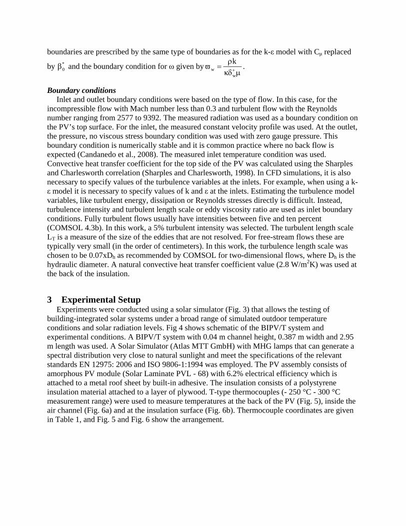
solid wall, for a turbulent flow, is different as compared to the free stream. In COMSOL, analytical expressions, known as wall functions are used to describe the flow at the walls. The wall functions in COMSOL multiphysics are such that the computational domain is assumed to start a distance δw from the wall as shown in Fig. 2 (COMSOL 4.3b).

Figure 2: The computational domain starts a distance δw from the wall for wall functions.

The distance δw is automatically computed so that

ww u+

τ

δδ = ρ

µ,

where 14u C kτ µ= is the friction velocity, which becomes 11.06 (COMSOL 4.3b). This

corresponds to the distance from the wall the logarithmic layer meets the viscous sub-layer. δw is limited from below so that it never becomes smaller than half of the height of the boundary mesh cell. w

+δ can become higher than 11.06 if the mesh is relatively coarse. In this work, w+δ was

maintained to the recommended value of 11.06 on of the walls. In case of the k-ω model wall

boundaries are prescribed by the same type of boundaries as for the k-ε model with Cμ replaced

by *0β and the boundary condition for ω given by w

w

k+

ρϖ =

κδ µ.

Boundary conditions Inlet and outlet boundary conditions were based on the type of flow. In this case, for the

incompressible flow with Mach number less than 0.3 and turbulent flow with the Reynolds number ranging from 2577 to 9392. The measured radiation was used as a boundary condition on the PV’s top surface. For the inlet, the measured constant velocity profile was used. At the outlet, the pressure, no viscous stress boundary condition was used with zero gauge pressure. This boundary condition is numerically stable and it is common practice where no back flow is expected (Candanedo et al., 2008). The measured inlet temperature condition was used. Convective heat transfer coefficient for the top side of the PV was calculated using the Sharples and Charlesworth correlation (Sharples and Charlesworth, 1998). In CFD simulations, it is also necessary to specify values of the turbulence variables at the inlets. For example, when using a k-ε model it is necessary to specify values of k and ε at the inlets. Estimating the turbulence model variables, like turbulent energy, dissipation or Reynolds stresses directly is difficult. Instead, turbulence intensity and turbulent length scale or eddy viscosity ratio are used as inlet boundary conditions. Fully turbulent flows usually have intensities between five and ten percent (COMSOL 4.3b). In this work, a 5% turbulent intensity was selected. The turbulent length scale LT is a measure of the size of the eddies that are not resolved. For free-stream flows these are typically very small (in the order of centimeters). In this work, the turbulence length scale was chosen to be 0.07xDh as recommended by COMSOL for two-dimensional flows, where Dh is the hydraulic diameter. A natural convective heat transfer coefficient value (2.8 W/m2K) was used at the back of the insulation.

3 Experimental Setup Experiments were conducted using a solar simulator (Fig. 3) that allows the testing of

building-integrated solar systems under a broad range of simulated outdoor temperature conditions and solar radiation levels. Fig 4 shows schematic of the BIPV/T system and experimental conditions. A BIPV/T system with 0.04 m channel height, 0.387 m width and 2.95 m length was used. A Solar Simulator (Atlas MTT GmbH) with MHG lamps that can generate a spectral distribution very close to natural sunlight and meet the specifications of the relevant standards EN 12975: 2006 and ISO 9806-1:1994 was employed. The PV assembly consists of amorphous PV module (Solar Laminate PVL - 68) with 6.2% electrical efficiency which is attached to a metal roof sheet by built-in adhesive. The insulation consists of a polystyrene insulation material attached to a layer of plywood. T-type thermocouples (- 250 °C - 300 °C measurement range) were used to measure temperatures at the back of the PV (Fig. 5), inside the air channel (Fig. 6a) and at the insulation surface (Fig. 6b). Thermocouple coordinates are given in Table 1, and Fig. 5 and Fig. 6 show the arrangement.

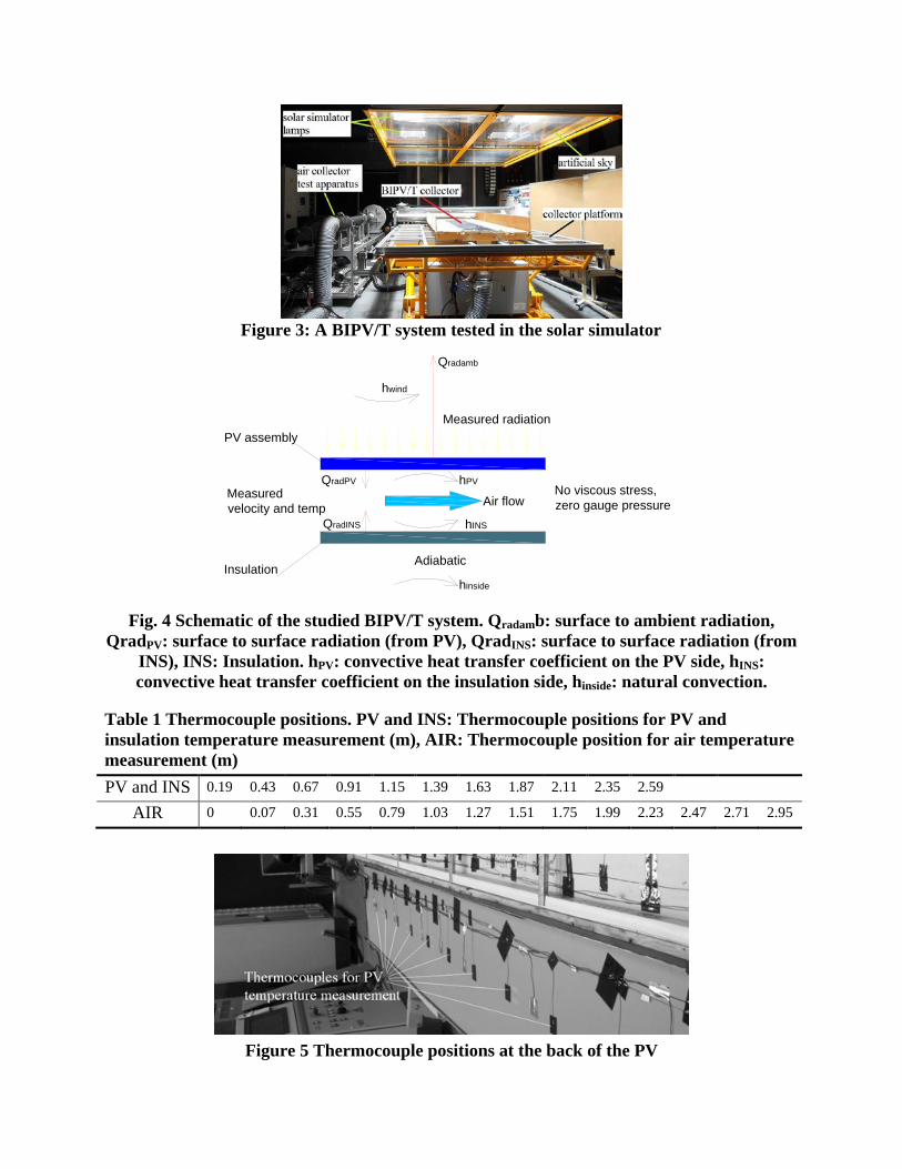
Figure 3: A BIPV/T system tested in the solar simulator

Fig. 4 Schematic of the studied BIPV/T system. Qradamb: surface to ambient radiation,

QradPV: surface to surface radiation (from PV), QradINS: surface to surface radiation (from INS), INS: Insulation. hPV: convective heat transfer coefficient on the PV side, hINS: convective heat transfer coefficient on the insulation side, hinside: natural convection.

Table 1 Thermocouple positions. PV and INS: Thermocouple positions for PV and insulation temperature measurement (m), AIR: Thermocouple position for air temperature measurement (m) PV and INS 0.19 0.43 0.67 0.91 1.15 1.39 1.63 1.87 2.11 2.35 2.59

AIR 0 0.07 0.31 0.55 0.79 1.03 1.27 1.51 1.75 1.99 2.23 2.47 2.71 2.95

Figure 5 Thermocouple positions at the back of the PV

Measured radiation

Measuredvelocity and temp

Adiabatic

hwind

hPV

hINS

Air flow

Insulation

PV assembly

No viscous stress,zero gauge pressure

QradPV

QradINS

Qradamb

hinside

The Kipp & Zonen pyranometer with spectral range of 310 - 2800 µm and solar irradiance measurement up to 4000 W/m² was used. Wind speed was measured with D12-65 transmitter series with a measurement range of 0 - 10 m/s with an accuracy of ±0.1 m/s. The air flow rate was measured with an orifice plate having a volumetric range of 30 - 530 m3/hr.

(a) (b) Figure 6 (a) Thermocouple in the middle of the channel for measuring air temperature and

(b) thermocouple for measuring insulation temperature

4 Results and Discussion

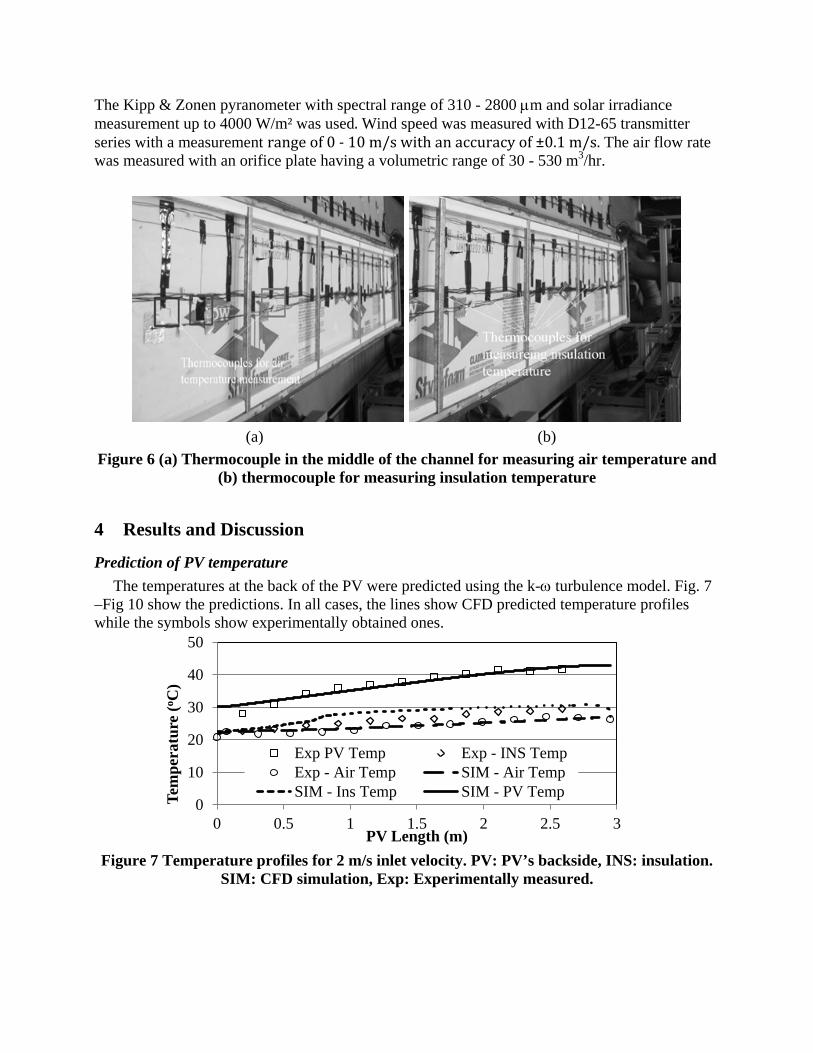
Prediction of PV temperature The temperatures at the back of the PV were predicted using the k-ω turbulence model. Fig. 7

–Fig 10 show the predictions. In all cases, the lines show CFD predicted temperature profiles while the symbols show experimentally obtained ones.

Figure 7 Temperature profiles for 2 m/s inlet velocity. PV: PV’s backside, INS: insulation.

SIM: CFD simulation, Exp: Experimentally measured.

0

10

20

30

40

50

0 0.5 1 1.5 2 2.5 3

Tem

pera

ture

(o C)

PV Length (m)

Exp PV Temp Exp - INS TempExp - Air Temp SIM - Air TempSIM - Ins Temp SIM - PV Temp

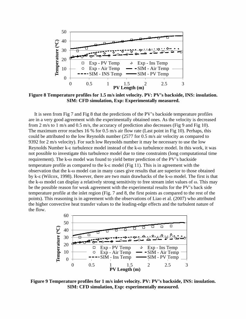
Figure 8 Temperature profiles for 1.5 m/s inlet velocity. PV: PV’s backside, INS: insulation.

SIM: CFD simulation, Exp: Experimentally measured.

It is seen from Fig 7 and Fig 8 that the predictions of the PV’s backside temperature profiles are in a very good agreement with the experimentally obtained ones. As the velocity is decreased from 2 m/s to 1 m/s and 0.5 m/s, the accuracy of prediction also decreases (Fig 9 and Fig 10). The maximum error reaches 16 % for 0.5 m/s air flow rate (Last point in Fig 10). Perhaps, this could be attributed to the low Reynolds number (2577 for 0.5 m/s air velocity as compared to 9392 for 2 m/s velocity). For such low Reynolds number it may be necessary to use the low Reynolds Number k-ε turbulence model instead of the k-ω turbulence model. In this work, it was not possible to investigate this turbulence model due to time constraints (long computational time requirement). The k-ω model was found to yield better prediction of the PV’s backside temperature profile as compared to the k-ε model (Fig 11). This is in agreement with the observation that the k-ω model can in many cases give results that are superior to those obtained by k-ε (Wilcox, 1998). However, there are two main drawbacks of the k-ω model. The first is that the k-ω model can display a relatively strong sensitivity to free stream inlet values of ω. This may be the possible reason for weak agreement with the experimental results for the PV’s back side temperature profile at the inlet region (Fig. 7 and 8, the first points as compared to the rest of the points). This reasoning is in agreement with the observations of Liao et al. (2007) who attributed the higher convective heat transfer values to the leading-edge effects and the turbulent nature of the flow.

Figure 9 Temperature profiles for 1 m/s inlet velocity. PV: PV’s backside, INS: insulation.

SIM: CFD simulation, Exp: experimentally measured.

0

10

20

30

40

50

0 0.5 1 1.5 2 2.5 3

Tem

pera

ture

(o C)

PV Length (m)

Exp - PV Temp Exp - Ins TempExp - Air Temp SIM - Air TempSIM - INS Temp SIM - PV Temp

0102030405060

0 0.5 1 1.5 2 2.5 3

Tem

pera

ture

(o C)

PV Length (m)

Exp - PV Temp Exp - Ins TempExp - Air Temp SIM - Air TempSIM - Ins Temp SIM - PV Temp

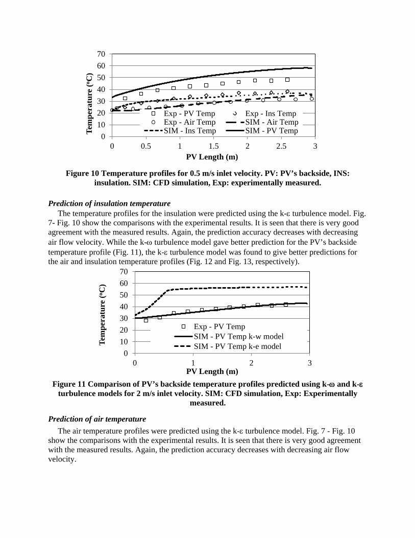
Figure 10 Temperature profiles for 0.5 m/s inlet velocity. PV: PV’s backside, INS:

insulation. SIM: CFD simulation, Exp: experimentally measured. Prediction of insulation temperature

The temperature profiles for the insulation were predicted using the k-ε turbulence model. Fig. 7- Fig. 10 show the comparisons with the experimental results. It is seen that there is very good agreement with the measured results. Again, the prediction accuracy decreases with decreasing air flow velocity. While the k-ω turbulence model gave better prediction for the PV’s backside temperature profile (Fig. 11), the k-ε turbulence model was found to give better predictions for the air and insulation temperature profiles (Fig. 12 and Fig. 13, respectively).

Figure 11 Comparison of PV’s backside temperature profiles predicted using k-ω and k-ε

turbulence models for 2 m/s inlet velocity. SIM: CFD simulation, Exp: Experimentally measured.

Prediction of air temperature The air temperature profiles were predicted using the k-ε turbulence model. Fig. 7 - Fig. 10

show the comparisons with the experimental results. It is seen that there is very good agreement with the measured results. Again, the prediction accuracy decreases with decreasing air flow velocity.

010203040506070

0 0.5 1 1.5 2 2.5 3

Tem

pera

ture

(o C)

PV Length (m)

Exp - PV Temp Exp - Ins TempExp - Air Temp SIM - Air TempSIM - Ins Temp SIM - PV Temp

010203040506070

0 1 2 3

Tem

pera

ture

(o C)

PV Length (m)

Exp - PV TempSIM - PV Temp k-w modelSIM - PV Temp k-e model

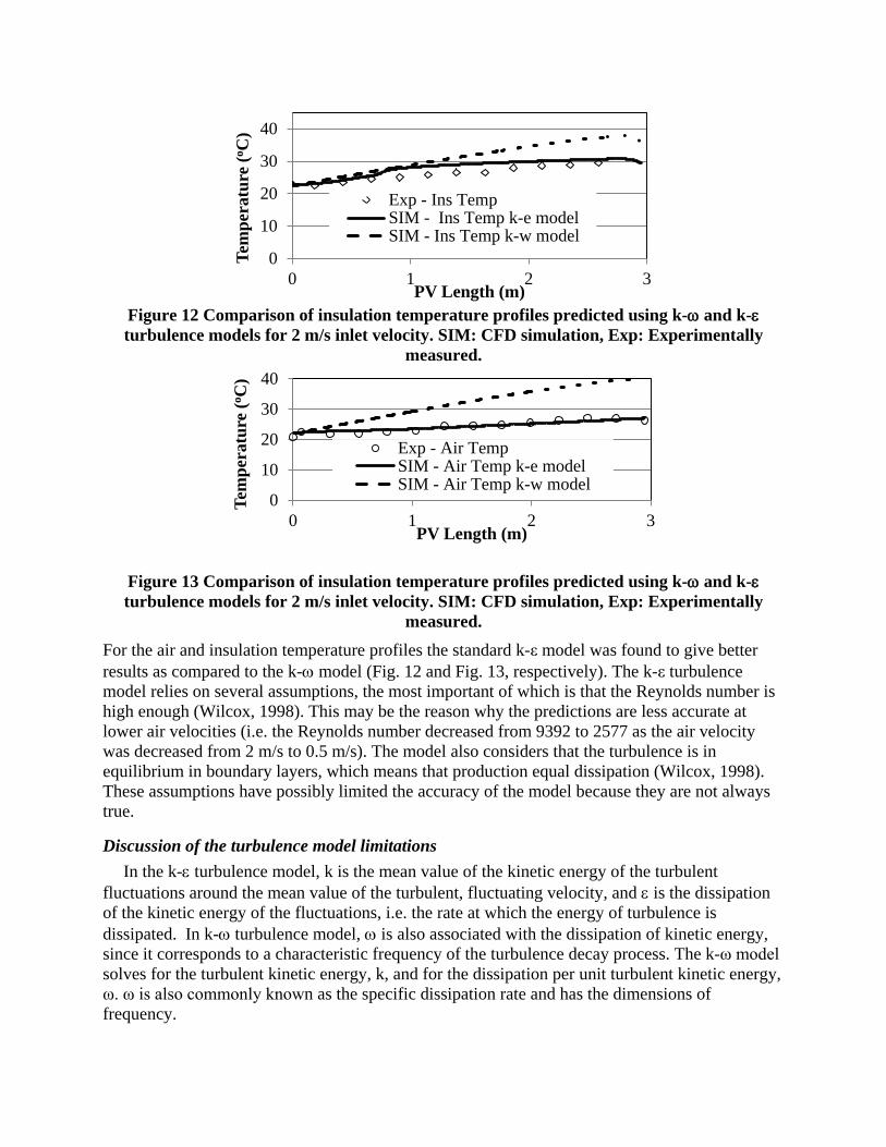
Figure 12 Comparison of insulation temperature profiles predicted using k-ω and k-ε turbulence models for 2 m/s inlet velocity. SIM: CFD simulation, Exp: Experimentally

measured.

Figure 13 Comparison of insulation temperature profiles predicted using k-ω and k-ε turbulence models for 2 m/s inlet velocity. SIM: CFD simulation, Exp: Experimentally

measured. For the air and insulation temperature profiles the standard k-ε model was found to give better results as compared to the k-ω model (Fig. 12 and Fig. 13, respectively). The k-ε turbulence model relies on several assumptions, the most important of which is that the Reynolds number is high enough (Wilcox, 1998). This may be the reason why the predictions are less accurate at lower air velocities (i.e. the Reynolds number decreased from 9392 to 2577 as the air velocity was decreased from 2 m/s to 0.5 m/s). The model also considers that the turbulence is in equilibrium in boundary layers, which means that production equal dissipation (Wilcox, 1998). These assumptions have possibly limited the accuracy of the model because they are not always true.

Discussion of the turbulence model limitations In the k-ε turbulence model, k is the mean value of the kinetic energy of the turbulent

fluctuations around the mean value of the turbulent, fluctuating velocity, and ε is the dissipation of the kinetic energy of the fluctuations, i.e. the rate at which the energy of turbulence is dissipated. In k-ω turbulence model, ω is also associated with the dissipation of kinetic energy, since it corresponds to a characteristic frequency of the turbulence decay process. The k-ω model solves for the turbulent kinetic energy, k, and for the dissipation per unit turbulent kinetic energy, ω. ω is also commonly known as the specific dissipation rate and has the dimensions of frequency.

0

10

20

30

40

0 1 2 3

Tem

pera

ture

(o C)

PV Length (m)

Exp - Ins TempSIM - Ins Temp k-e modelSIM - Ins Temp k-w model

0

10

20

30

40

0 1 2 3

Tem

pera

ture

(o C)

PV Length (m)

Exp - Air TempSIM - Air Temp k-e modelSIM - Air Temp k-w model

In the k-ε model, the eddy viscosity is determined from a single turbulence length scale. The calculated turbulent diffusion occurs only at the specified scale, whereas in reality all scales contribute to the turbulent diffusion. It is also important that the turbulence is in equilibrium in boundary layers, which means that production equal dissipation. These and high Reynolds number assumptions limit the accuracy of the model because they are not always true. It does not, for example, respond correctly to flows with adverse pressure gradients (COMSOL 4.3b).

The k-ω model allows for a more accurate near wall treatment (COMSOL 4.3b). Although the k-ω turbulence model performs much better than k-ε for boundary layer flows with strong wall effects and separation, it can be sensitive to the free-stream value of ω. Possibly, this is the reason why the k-ω performs well for prediction of temperature profiles near the PV’s backside where there is high temperature gradient and wall effects are pronounced, while the k-ε model is better suited for the free-stream flow in the middle of the channel. Probably, on the insulation side, a leading-edge effect may have made the prediction less accurate when the k-ω model turbulence was used (Liao et al. (2007)).

5 Conclusions CFD study of BIPV/T systems with forced convection of air with various air flow rates (air

velocities) was conducted to predict temperatures profiles of the back of the PV, the flowing air in the middle of the channel and the insulation; and to investigate the accuracy of predictions of the k-ε and k-ω turbulence models. The k-ω model yielded the best agreement with the measured PV backside temperature profiles. The k-ε model yielded the best agreement with the measured air temperature and the insulation temperature profiles. The agreement indicates that it is possible to use the CFD predicted temperature profiles to obtain relationships between the average convective heat transfer coefficients and velocity. The relationships obtained will be useful for the development of simple mathematical models that facilitate the design and optimization of different parts of the BIPV/T system. 6 Acknowledgments The authors gratefully acknowledge the financial support of the Natural Sciences and Engineering Research Council of Canada (NSERC), Toronto Atmospheric Fund (TAF), MITACS, Ryerson University and Concordia University.

7 References Candanedo, J. and A.K., Athienitis 2008. Simulation of the Performance of a BIPV/T system

coupled to a Heat Pump in a Residential Heating Application. In Proc. of the 9th International Heat Pump Conference, Zürich, Switzerland.

Candanedo, J. and Athienitis, A. K. 2010. A Simulation Study of Anticipatory Control Strategies in a Net Zero Energy Solar House. ASHRAE Trans., 116(1): 246-259.

Candanedo, L., O’Brien, W. and Athienitis, A.K. 2009. Development of an air-based building-integrated photovoltaic-thermal system model. In 11th International IBPSA conference, Glasgw, Scotland, July 27-30.

Candanedo, L.M., C. Diarra, A. Athienitis, and S. Harrison. 2008. Numerical modelling of heat transfer in photovoltaic-thermal air-based systems. In 3rd SBRN and SESCI 33rd Joint Conference, Fredericton, Canada.

Cartmell, B.P., Shankland, N.J., Fiala, D., Hanby V. 2004. A multi-operational ventilated photovoltaic and solar air collector: application, simulation and initial monitoring feedback. Solar Energy 76: 45–53.

Charron, R. and Athienitis, A. K. 2006. A Two-Dimensional model of a double-façade with integrated photovoltaic panels. ASME J. Sol. Energy Eng. 128: 160–167.

Charron, R., and Athienitis, A. K. 2006. Optimization of the performance of double-façades with integrated photovoltaic panels and motorized blinds. Sol. Energy 80 (5): 482–491.

Chen Y., Athienitis A.K., Galal K.E. and Y. Poissant, 2007. Design and Simulation for a Solar House with BIPV/T System and Thermal Storage. In ISES Solar World Congress I: 327-332, 2007. Beijing, China,

Chen, Y. K., Galal and A. K., Athienitis 2010. Modeling, design and thermal performance of a BIPV/T system thermally coupled with a ventilated concrete slab in a low energy solar house: Part 2, ventilated concrete slab. Solar Energy 84(11): 1908-1919.

Chen, Y., Athienitis, A.K. and Galal, K.E. 2010. Modeling, design and thermal performance of a BIPV/T system thermally coupled with a ventilated concrete slab in a low energy solar house: Part 1, BIPV/T system and house energy concept. Solar Energy 84(11): 1892-1907.

Chow, T.T., He, W., and Ji, J. 2007. An experimental study of façade-integrated photovoltaic/water-heating system. Applied Thermal Engineering: 27 37-45.

Clarke, J.A., Hand, J.W., Johnstone, C.M., Kelly, N., and Strachan, P.A. 1996. Renewable Energy 8: 475-479.

COMSOL 4.3b documentation. Corbin, C. D. and Zhai, Z. J. 2010. Experimental and numerical investigation on thermal and

electrical performance of a building integrated photovoltaic-thermal collector system. Energy and Buildings 42: 76-82.

Dembo, A., Fung, A., Ng K.L.R. and Pyrka, A. 2010. The Archetype Sustainable House: Investigating its potentials to achieving the net-zero energy status based on the results of a detailed energy audit. In International High Performance Buildings Conference 2010, Purdue University.

Gan, G., Riffat S. B. 2004. CFD modelling of air flow and thermal performance of an atrium integrated with photovoltaics. Building and Environment 39: 735-748.

Getu, H., and Fung, A. 2014. Building Integrated Photovoltaic/Thermal Façade with Forced Ventilation and Natural Convection. ASHRAE Transactions 120, Part 1.

Getu, H., Fung, A., P. Dash 2013. Simplified Approach to Thermal Modeling of a Building Integrated Photovoltaic/thermal Façade. In Proceedings of CCTC 2013, Montreal, Canada, May 27 –29.

Infield, D., Eicker, U., Fux, Mei, L. and Schumacher J. 2006. A simplified approach to thermal performance calculation for building integrated mechanical ventilated PV facades. Building and Environment 41: 893-901.

Infield, D., Mei, L. and Eicker, U. 2004. Thermal performance estimation for ventilated PV façade. Solar Energy 76: 93-98.

Liao, L., Athienitis, A. K., Candanedo, L., Park, K. W., Poissant, Y. and Collins, M. 2007. Numerical and experimental study of heat transfer in a BIPV-thermal system. Journal of Solar Engineering 129: 423-430.

Mei, L., Infield, D., Eicker, U. and Fux, V. 2003. Thermal modeling of a building with an integrated ventilated PV façade. Energy and Buildings 35: 605-617.

Naewngerndee, R., Hattha, E., Chumpolrat, K., Sangkapes, T., Phongsitong, J. and Jaikla, S., 2011. Finite element method for computational fluid dynamics to design photovoltaic thermal (PV/T) system configuration .Solar Energy Materials & Solar Cells 95 (1): 390-393.

Pantic, S., Candanedo, L. and Athienitis, A.K., 2010. Modeling of energy performance of a house with three configurations of building-integrated photovoltaic/thermal systems, Energy and Buildings 42: 1779-1789.

Patankar, S.V. 1980. Numerical Heat Transfer and Fluid Flow, Hemisphre Publishing Corporation.

Safa, A. A., 2012. Performance Analysis of a Two-stage Variable Capacity Air Source Heat Pump and A Horizontal Loop Coupled Ground Source Heat Pump System. MASc thesis, Mechanical and Industrial Engineering, Ryerson University.

Sharples, S. and Charlesworth, P.S. 1998. Full-scale measurements of wind induced convective heat transfer from a roof-mounted flat plate solar collector. Solar Energy 62: 69-77.

Solar Energy Perspectives: Executive Summary, International Energy Agency. 2011. Wilcox, D.C., 1998. Turbulence Modeling for CFD 2nd ed., DCW Industries.

We thank the reviewers’ for their valuable comments. We have addressed their concerns as follows, in italics.

Reviewer A: Comments for author: Major concerns: This case study has significantly low Reynolds numbers. The flow is most likely in transition from laminar to turbulent regime for V=0.5m/s. The accuracy of most RANS turbulence models such as standard k-epsilon reduces as the Reynolds number decreases and they are not valid when the flow field is not fully turbulent. This explains the deviations from experiment. In principle, CFD with a RANS turbulence model is not a predictive tool for such a flow field (specially the case with Re = 2577). Authors need to tone down their conclusion. Yes, the accuracy of most RANS turbulence models such as standard k-epsilon reduces as the Reynolds number decreases. We agree with the reviewer’s concerns and we were aware of it issue and we had stated this possibility in two places as follows: “As the velocity is decreased from 2 m/s to 1 m/s and 0.5 m/s, the accuracy of prediction also decreases (Fig 8 and Fig 9). Perhaps, this could be attributed to the low Reynolds number (2577 for 0.5 m/s air velocity as compared to 9392 for 2 m/s velocity). For such low Reynolds number it may be necessary to use the low Reynolds Number k-ε turbulence model instead of the k-ω turbulence model. In this work, it was not possible to investigate this turbulence model due to time constraints (long computational time requirement).” in Section 4, in the paragraph just after Fig. 7 “The k-ε turbulence model relies on several assumptions, the most important of which is that the Reynolds number is high enough (Wilcox, 1998). This may be the reason why the predictions are less accurate at lower air velocities (i.e. the Reynolds number decreased from 9392 to 2577 as the air velocity was decreased from 2 m/s to 0.5 m/s).” in the paragraph above Section 5. In the future we plan to investigate the problem using Low-Reynolds Number k-epsilon turbulence model for this case (i.e. 0.5 m/s air velocity). Minor Comments: 1. The left-hand side of equation (3) is wrong. Also, does COMSOL solve an equation for temperature or enthalpy? We have corrected the equation. The Heat Transfer in Fluids physics solves this equation for the temperature, T. The second part of the question is not clear. If the reviewer’s question was meant to say if COMSOL can analyze heat conduction with phase change, then the answer is YES. According to COMSOL 4.3b manual, the heat transfer with phase change node is used to solve the heat equation after specifying the properties of a phase change material according to the apparent heat capacity formulation. Instead of adding a latent heat L in the energy balance equation when the material reaches its phase change temperature Tpc, it is assumed that the transformation occurs in a temperature interval between Tpc − ΔT/2 and Tpc + ΔT/2. In this interval, the material phase is modeled by a smoothed function, α, representing the fraction of phase after transition, which is equal to 0 before Tpc − ΔT/2 and to 1 after Tpc + ΔT/2. 2. Authors did not mention anything about turbulence wall functions. In order to obtain the right

convective heat transfer coefficient, one needs to use turbulent wall functions. Even if the wall boundary layer is resolved (y+ < 5), the underlying turbulence model has an inherent high-Reynolds number assumption that does not provide enough dissipation near the wall. We have added the following entire Section on Wall Functions “The assumptions used to derive the k-ε model are not valid close to walls because the flow close to a solid wall, for a turbulent flow is different as compared to the free stream. In COMSOL, analytical expressions, known as wall functions are used to describe the flow at the walls. The wall functions in COMSOL Multiphysics are such that the computational domain is assumed to start a distance δw from the wall as shown in Fig. 2 (COMSOL 4.3b).

Figure 2: The computational domain starts a distance δw from the wall for wall functions.

The distance δw is automatically computed so that

ww u+

τ

δδ = ρ

µ,

where 14u C kτ µ= is the friction velocity, which becomes 11.06 (COMSOL 4.3b). This

corresponds to the distance from the wall the logarithmic layer meets the viscous sub-layer. δw is limited from below so that it never becomes smaller than half of the height of the boundary mesh cell. w

+δ can become higher than 11.06 if the mesh is relatively coarse. In this work, w+δ = 11.06

on of the walls as recommended by COMSOL. In case of the k-ε model wall boundaries are prescribed by the same type of boundaries as for the k-ε model with Cμ replaced by *

0β and the

boundary condition for ω given by ww

k+

ρϖ =

κδ µ.”

3.Please add explanations for what the solid line and dashed line represent in Fig.7. and Fig.9 We have fixed this mistake. 4.Please correct the captions for Fig.9. The velocity is 0.5 m/s not 1m/s We have fixed this mistake. 5.Please correct the legend for Fig. 11. It reads “Exp - Ins Temp k-e model” We have fixed this mistake.

Reviewer C: Comments for author: - Carefully check the grammar of your paper. We have gone through the entire paper to correct grammatical mistakes to the best of our abilities. - Could you describe, briefly, the differences between k-e and k-w turbulence models in terms of accuracy or applicability to your problem? What makes k-w approximate the PV temperature better than the k-e model? What makes k-e approximate the insulation/air temperature better? I find this discussion much more relevant than including the explicit formulas for each model. We have added a discussion Section just above Section 5, which reads as follows “Discussion of the turbulence model limitations In the k-ε turbulence model, k is the mean value of the kinetic energy of the turbulent fluctuations around the mean value of the turbulent, fluctuating velocity and e is the dissipation of the kinetic energy of the fluctuations, i.e. the rate at which the energy of turbulence is dissipated. In k-ω turbulence model, ω is also associated with the dissipation of kinetic energy, since it corresponds to a characteristic frequency of the turbulence decay process. The k-ω model solves for the turbulent kinetic energy, k, and for the dissipation per unit turbulent kinetic energy, ω. ω is also commonly known as the specific dissipation rate and has the dimensions of frequency. In the k-e model, the eddy viscosity is determined from a single turbulence length scale. The calculated turbulent diffusion occurs only at the specified scale, whereas in reality all scales contribute to the turbulent diffusion. It is also important that the turbulence is in equilibrium in boundary layers, which means that production equal dissipation. These and high Reynolds number assumptions limit the accuracy of the model because they are not always true. It does not, for example, respond correctly to flows with adverse pressure gradients (COMSOL 4.3b). The k-ω model allows for a more accurate near wall treatment (COMSOL 4.3b). Although the k-ω turbulence model performs much better than k-ε for boundary layer flows with strong wall effects and separation, it can be sensitive to the free-stream value of ω. Possibly this could be the reason why the k-w performs well for prediction of temperature profiles near the PV’s backside where there is high temperature gradient and wall effects are pronounced, while the k-e model is better suited for the free-stream flow in the middle of the channel. Probably, on the insulation side, a leading-edge effect may have made the prediction less accurate when the k-w model turbulence was used (Liao et al. (2007)).” - You claim, "The agreement indicates that it is possible to use the CFD predicted temperature profiles to obtain relationships between the average convective heat transfer coefficients and velocity, without conducting extensive and costly experimental measurements," but you did perform an experimental measurement without which you could not have identified the substantial errors in the k-w and k-e model simulations. I think this bears some discussion. We have removed “without conducting extensive and costly experimental measurements.” from the manuscript.