Computational Finance - Northwestern University

Volume 11 Number 4Summer 2008

The Jo

urn

al of C

om

pu

tation

al Finan

ce Volum

e 11 Num

ber 4 Summ

er 2008

Incisive Media, Haymarket House, 28-29 Haymarket, London SW1Y 4RX

The Journal of

ComputationalFinance

n An adaptive procedure for estimating coherent risk measures based on generalized scenarios Vadim Lesnevski, Barry L. Nelson and Jeremy Staum

n Pricing options on realized variance in the Heston model with jumps in returns and volatility Artur Sepp

n Robust active portfolio management Emre Erdogan, Donald G. Goldfarb and Garud Iyengar

n Optimal portfolio management in markets with asymmetric taxation Cristin Buescu and Michael Taksar

The Journal of Computational Finance (1–31) Volume 11/Number 4, Summer 2008

An adaptive procedure for estimatingcoherent risk measures based ongeneralized scenarios

Vadim LesnevskiRoyal Bank of Scotland, Global Banking & Markets, 250 Bishopsgate,London EC2M 4AA, UK; email: [email protected]

Barry L. NelsonDepartment of Industrial Engineering and Management Sciences, Northwestern University,Evanston, IL, USA; email: [email protected]

Jeremy StaumDepartment of Industrial Engineering and Management Sciences, Northwestern University,Evanston, IL, USA; email: [email protected]

Simulating coherent risk measures is potentially very computationallyexpensive. We present a procedure for generating a fixed-width confidenceinterval for a coherent risk measure based on a finite number of generalizedscenarios. Computational experiments show that this procedure is muchmore efficient than standard methods, making simulation of coherent riskmeasures based on even a large number of generalized scenarios afford-able. The procedure improves upon previous specialized methods by beingreliably efficient when applied to simulation of generalized scenarios andportfolios with heterogeneous characteristics. We also show how robust theprocedure’s performance is to violations of the normality assumption underwhich its statistical validity is proved, and study the magnitude of estimationerror.

1 INTRODUCTION

Coherent risk measures can improve the practice of risk management (Artzneret al (1999)) and pricing derivative securities (Jaschke and Küchler (2001); Staum(2004)). In some cases, coherent risk measures may need to be estimated bysimulation. In such cases, especially for large firm-wide risk measurement prob-lems, carrying out the simulation by standard methods could be much slower thansimulations currently used in risk management and derivatives pricing, and too slowfor routine use in practice.

This material is based upon work supported by the National Science Foundation under grantsNo. DMI-0217690, DMS-0202958 and DMI-0555485. Part of this material has been publishedin the Proceedings of the 2006 Winter Simulation Conference. We thank the Editor-in-Chief andan anonymous referee for their helpful comments that have led to an improved and expandedpresentation.

1

2 V. Lesnevski et al

To see why, consider that any coherent risk measure ρ has a representation ofthe form:

ρ(Y )= supP∈P

EP[−Y/r] (1)

where Y is the value of a portfolio at a future time horizon, r is a stochasticdiscount factor that represents the time value of money and P is a set of probabilitymeasures (Artzner et al (1999, Proposition 4.1)). Equations of a similar form holdfor the related problems in derivative security pricing. We simplify the problemsomewhat by limiting our analysis to the case where the set P has only a finitenumber k of elements P1, P2, . . . , Pk . The obvious way of estimating ρ(Y ) bysimulation is to estimate EPi

[−Y/r] for each i = 1, 2, . . . , k, which is typicallyabout k times as expensive as estimating a single expectation by simulation. Thismay be impractically expensive when Y is the value of a portfolio that containsthousands of derivative securities and Pi represents a model governing hundreds ofunderlying risk factors.

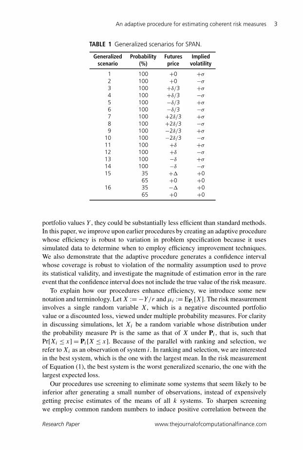
The assumption that P = {P1, P2, . . . , Pk} holds, for instance, when thedecision-maker designs the coherent risk measure (or the underlying acceptanceset, in the case of derivative security pricing) by specifying these k generalizedscenarios. The SPAN margin computation system of the Chicago MercantileExchange is closely related to such a risk measure. To simplify the example, weconsider applying SPAN to a portfolio involving a futures contract for deliveryin a single month and options on that contract. In this case, our risk measure hask = 16 generalized scenarios, which involve the changes over one day in the futuresprice and in the implied volatility of the options. They are based on a hypotheticalmoderate move δ or an extreme move � in the futures price and a hypotheticalchange σ in the implied volatility, as illustrated in Table 1. The first 14 probabilitymeasures are degenerate: each of them is a point mass on one scenario. The 15th and16th probability measures place 35% probability on an extreme move in the futuresprice and 65% probability on no change; the expected loss under these probabilitymeasures is close to 35% of the loss in the case of an extreme move, which SPANuses. The maximum expected loss over all generalized scenarios is used to computemargin requirements for the portfolio of futures and options.

The assumption that P is finite does not generally hold for worst conditionalexpectation (Artzner et al (1999, Section 5)) or related risk measures such as tailconditional expectation, conditional value-at-risk and expected shortfall (see Acerbiand Tasche (2002)). However, our procedure may provide a foundation for furtherwork on efficiently simulating worst conditional expectation. For coherent riskmeasures such that P is infinite, it may also be possible to use our procedure byapproximating P by the convex hull of k probability measures.

In Lesnevski et al (2007), we used tools from the ranking and selection literatureto create efficient procedures that generate a fixed-width confidence interval fora coherent risk measure. Those procedures were usually no more than twiceas expensive as estimating a single expectation by simulation, not k times asexpensive; in some cases, they were as little as 5% more expensive. However,those procedure have a weakness: for some problems, that is, for some sets P and

The Journal of Computational Finance Volume 11/Number 4, Summer 2008

An adaptive procedure for estimating coherent risk measures 3

TABLE 1 Generalized scenarios for SPAN.

Generalized Probability Futures Impliedscenario (%) price volatility

1 100 +0 +σ

2 100 +0 −σ

3 100 +δ/3 +σ

4 100 +δ/3 −σ

5 100 −δ/3 +σ

6 100 −δ/3 −σ

7 100 +2δ/3 +σ

8 100 +2δ/3 −σ

9 100 −2δ/3 +σ

10 100 −2δ/3 −σ

11 100 +δ +σ

12 100 +δ −σ

13 100 −δ +σ

14 100 −δ −σ

15 35 +� +065 +0 +0

16 35 −� +065 +0 +0

portfolio values Y , they could be substantially less efficient than standard methods.In this paper, we improve upon earlier procedures by creating an adaptive procedurewhose efficiency is robust to variation in problem specification because it usessimulated data to determine when to employ efficiency improvement techniques.We also demonstrate that the adaptive procedure generates a confidence intervalwhose coverage is robust to violation of the normality assumption used to proveits statistical validity, and investigate the magnitude of estimation error in the rareevent that the confidence interval does not include the true value of the risk measure.

To explain how our procedures enhance efficiency, we introduce some newnotation and terminology. Let X := −Y/r and µi := EPi

[X]. The risk measurementinvolves a single random variable X, which is a negative discounted portfoliovalue or a discounted loss, viewed under multiple probability measures. For clarityin discussing simulations, let Xi be a random variable whose distribution underthe probability measure Pr is the same as that of X under Pi , that is, such thatPr[Xi ≤ x] = Pi[X ≤ x]. Because of the parallel with ranking and selection, werefer to Xi as an observation of system i. In ranking and selection, we are interestedin the best system, which is the one with the largest mean. In the risk measurementof Equation (1), the best system is the worst generalized scenario, the one with thelargest expected loss.

Our procedures use screening to eliminate some systems that seem likely to beinferior after generating a small number of observations, instead of expensivelygetting precise estimates of the means of all k systems. To sharpen screeningwe employ common random numbers to induce positive correlation between the

Research Paper www.thejournalofcomputationalfinance.com


systems and thereby reduce the variance of their differences: see Glasserman (2004,pp. 361, 380) or Law and Kelton (2000). To reduce the number of replicationsrequired for estimation, we employ control-variate estimators to exploit strongcorrelation between the response of interest, X, and a vector C of randomvariables with known expectations, called control variates: see Glasserman (2004,Section 4.1) or Law and Kelton (2000).

A disadvantage of the procedures presented in Lesnevski et al (2007) is that insome cases the user might need to choose the procedure or its parameters basedon previous knowledge about the problem to gain efficiency. For example, having alarge screening budget is usually good, as it allows the procedure to screen out mostof the inferior systems. However, it might significantly decrease efficiency if morethan one system has the maximum mean, or if some systems are nearly tied withthe best. In such situations, screening might not be able to eliminate all systemsbut one, and the work done during screening might be more than is necessary toestimate the coherent risk measure accurately.

One of the procedures in Lesnevski et al (2007) uses the technique of “restart-ing”, in which data that is used for screening are subsequently discarded so asto make it possible to reduce the required sample sizes for the systems thatsurvive screening. The advantage of restarting is that the new data is statisticallyindependent of the screening exercise, so one may ignore the measures that werescreened out, and design for the smaller problem. Even though the procedure withrestarting is usually preferable over other alternatives, if screening is ineffective,restarting is wasteful of data. Without restarting, information generated duringscreening is reused during estimation of the confidence interval, so the only dangerof a large screening budget is that it might exceed the sample size required foraccurate estimation. With restarting, information generated during screening isthrown away, so it is important to make sure that no excess work is done duringscreening. Before running the simulation, the user would have to decide whether ornot to use restarting and how much data to allocate to the screening stage. Making agood decision without substantial experience with simulation problems of the sameform is difficult. In this paper we develop an adaptive multi-stage procedure that isreliably efficient. It gains the benefits of restarting and of having a large budgetto use for screening by restarting when simulated data suggests that restartingis worthwhile, rather than at a prespecified time that might be disadvantageous.With the adaptive procedure, the user does not have to guess whether or not to userestarting or what the screening budget should be.

In Section 2, we present motivating examples in which coherent risk measuresare estimated. The computational experiments that illustrate the procedure’s per-formance are carried out with these examples. Section 3 describes our adaptiveprocedure and gives a heuristic justification of its design, while the proof of itsstatistical validity is in Appendix A. Computational experiments demonstratingthe procedure’s efficiency are described in Section 4, while Sections 5 and 6feature experiments that test the robustness of the confidence interval’s coverageto non-normal data and explore the severity of error in the unlikely event that theconfidence interval does not contain the true value. Section 7 concludes the paper.



2 MOTIVATING EXAMPLES

We will test the performance of our procedures on two examples, which were alsoused in Lesnevski et al (2007). We selected these examples because it is easy tofind the true best mean, which we must do to study the coverage of the confidenceinterval that the procedure produces, but we believe that these examples have astructure similar to that of problems in which estimating the true best mean (worstexpected loss) would be a significant challenge.

2.1 Basket put

The first problem is to price a basket put option, whose payout at a terminal time T

is max{0, K −w′S(T )}, where K is the strike price, w is a vector of weights andS(T ) is the vector of terminal prices of the securities in the basket. The underlyingsecurity price vector S obeys the Black–Scholes model, so the price of the basketput price is its risk-neutral expected discounted payout.

Under the Black–Scholes model, the price vector S follows multivariate geomet-ric Brownian motion with risk-neutral drift r , the risk-free interest rate, and withcovariance matrix �. That is, ln Sj (T )= ln Sj (0)+ (r − ‖Aj‖2/2)T +AjZ

√T ,

where A is a matrix satisfying AA′ =�, ‖Aj‖ is the Euclidean norm of its j th row,ie, the volatility of the j th asset, and Z is a multivariate standard normal randomvector. The short-term interest rate r is observable, and there are standard methodsfor calibrating the underlying securities’ individual volatilities ‖Aj‖, whether fromhistorical data or by fitting to observable prices of market-traded options on theunderlying securities: see Cont and Tankov (2004, Chs 7, 13) and Shiryaev (1999,Ch. IV). However, estimation of the non-diagonal elements of � poses a greaterproblem. For pricing the basket put, the crucial quantity is ‖w′A‖, the volatilityof the basket, and this depends strongly on the correlations between assets. Theremay be a range of plausible correlations and thus a range of plausible prices for thebasket put.

In this example, the basket is a weighted average of three security prices withweights w1 = 0.5, w2 = 0.3 and w3 = 0.2. The initial security prices are all 100,and the strike price is K = 85. The interest rate r = 5% and the volatilities are‖A1‖ = 40%, ‖A2‖ = 30% and ‖A3‖ = 20%. To account for uncertainty aboutcorrelations, we use the k = 43 = 64 probability measures produced by allowingeach of the three pairwise correlations to be 0.2, 0.35, 0.55 or 0.75. Althoughthe payout in this example is far from normally distributed, the sample averagesare approximately normally distributed and the minimum coverage guarantees theconfidence limits held in all our experiments.

The three control variates used in this example are the discounted payouts ofput options with strike K on each individual asset in the basket. Their means aregiven by the Black–Scholes pricing formula, based on the known volatilities. Theidea behind using them as control variates is that much of the (unknown) error inestimating the basket put’s expected discounted payout can be explained as a linearfunction of the differences between the discounted payouts of the puts on individual



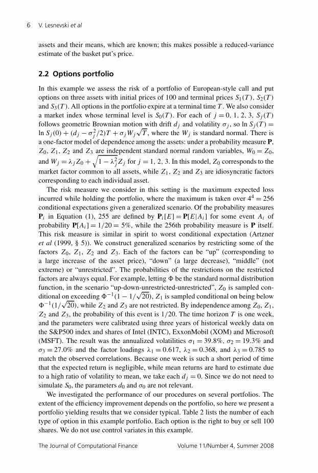
assets and their means, which are known; this makes possible a reduced-varianceestimate of the basket put’s price.

2.2 Options portfolio

In this example we assess the risk of a portfolio of European-style call and putoptions on three assets with initial prices of 100 and terminal prices S1(T ), S2(T )

and S3(T ). All options in the portfolio expire at a terminal time T . We also considera market index whose terminal level is S0(T ). For each of j = 0, 1, 2, 3, Sj (T )

follows geometric Brownian motion with drift dj and volatility σj , so ln Sj(T )=ln Sj(0)+ (dj − σ 2

j /2)T + σjWj

√T , where the Wj is standard normal. There is

a one-factor model of dependence among the assets: under a probability measure P,Z0, Z1, Z2 and Z3 are independent standard normal random variables, W0 = Z0,

and Wj = λjZ0 +√

1− λ2jZj for j = 1, 2, 3. In this model, Z0 corresponds to the

market factor common to all assets, while Z1, Z2 and Z3 are idiosyncratic factorscorresponding to each individual asset.

The risk measure we consider in this setting is the maximum expected lossincurred while holding the portfolio, where the maximum is taken over 44 = 256conditional expectations given a generalized scenario. Of the probability measuresPi in Equation (1), 255 are defined by Pi[E] = P[E|Ai] for some event Ai ofprobability P[Ai] = 1/20= 5%, while the 256th probability measure is P itself.This risk measure is similar in spirit to worst conditional expectation (Artzneret al (1999, § 5)). We construct generalized scenarios by restricting some of thefactors Z0, Z1, Z2 and Z3. Each of the factors can be “up” (corresponding toa large increase of the asset price), “down” (a large decrease), “middle” (notextreme) or “unrestricted”. The probabilities of the restrictions on the restrictedfactors are always equal. For example, letting � be the standard normal distributionfunction, in the scenario “up-down-unrestricted-unrestricted”, Z0 is sampled con-ditional on exceeding �−1(1− 1/

√20), Z1 is sampled conditional on being below

�−1(1/√

20), while Z2 and Z3 are not restricted. By independence among Z0, Z1,Z2 and Z3, the probability of this event is 1/20. The time horizon T is one week,and the parameters were calibrated using three years of historical weekly data onthe S&P500 index and shares of Intel (INTC), ExxonMobil (XOM) and Microsoft(MSFT). The result was the annualized volatilities σ1 = 39.8%, σ2 = 19.3% andσ3 = 27.0% and the factor loadings λ1 = 0.617, λ2 = 0.368, and λ3 = 0.785 tomatch the observed correlations. Because one week is such a short period of timethat the expected return is negligible, while mean returns are hard to estimate dueto a high ratio of volatility to mean, we take each dj = 0. Since we do not need tosimulate S0, the parameters d0 and σ0 are not relevant.

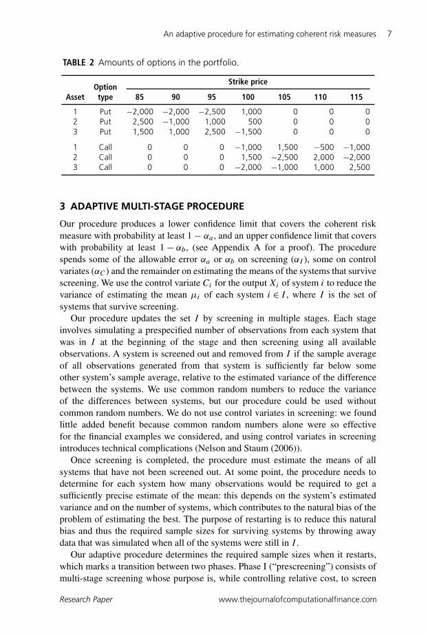
We investigated the performance of our procedures on several portfolios. Theextent of the efficiency improvement depends on the portfolio, so here we present aportfolio yielding results that we consider typical. Table 2 lists the number of eachtype of option in this example portfolio. Each option is the right to buy or sell 100shares. We do not use control variates in this example.



TABLE 2 Amounts of options in the portfolio.

Strike priceOption

Asset type 85 90 95 100 105 110 115

1 Put −2,000 −2,000 −2,500 1,000 0 0 02 Put 2,500 −1,000 1,000 500 0 0 03 Put 1,500 1,000 2,500 −1,500 0 0 0

1 Call 0 0 0 −1,000 1,500 −500 −1,0002 Call 0 0 0 1,500 −2,500 2,000 −2,0003 Call 0 0 0 −2,000 −1,000 1,000 2,500

3 ADAPTIVE MULTI-STAGE PROCEDURE

Our procedure produces a lower confidence limit that covers the coherent riskmeasure with probability at least 1− αa , and an upper confidence limit that coverswith probability at least 1− αb, (see Appendix A for a proof). The procedurespends some of the allowable error αa or αb on screening (αI ), some on controlvariates (αC) and the remainder on estimating the means of the systems that survivescreening. We use the control variate Ci for the output Xi of system i to reduce thevariance of estimating the mean µi of each system i ∈ I , where I is the set ofsystems that survive screening.

Our procedure updates the set I by screening in multiple stages. Each stageinvolves simulating a prespecified number of observations from each system thatwas in I at the beginning of the stage and then screening using all availableobservations. A system is screened out and removed from I if the sample averageof all observations generated from that system is sufficiently far below someother system’s sample average, relative to the estimated variance of the differencebetween the systems. We use common random numbers to reduce the varianceof the differences between systems, but our procedure could be used withoutcommon random numbers. We do not use control variates in screening: we foundlittle added benefit because common random numbers alone were so effectivefor the financial examples we considered, and using control variates in screeningintroduces technical complications (Nelson and Staum (2006)).

Once screening is completed, the procedure must estimate the means of allsystems that have not been screened out. At some point, the procedure needs todetermine for each system how many observations would be required to get asufficiently precise estimate of the mean: this depends on the system’s estimatedvariance and on the number of systems, which contributes to the natural bias of theproblem of estimating the best. The purpose of restarting is to reduce this naturalbias and thus the required sample sizes for surviving systems by throwing awaydata that was simulated when all of the systems were still in I .

Our adaptive procedure determines the required sample sizes when it restarts,which marks a transition between two phases. Phase I (“prescreening”) consists ofmulti-stage screening whose purpose is, while controlling relative cost, to screen



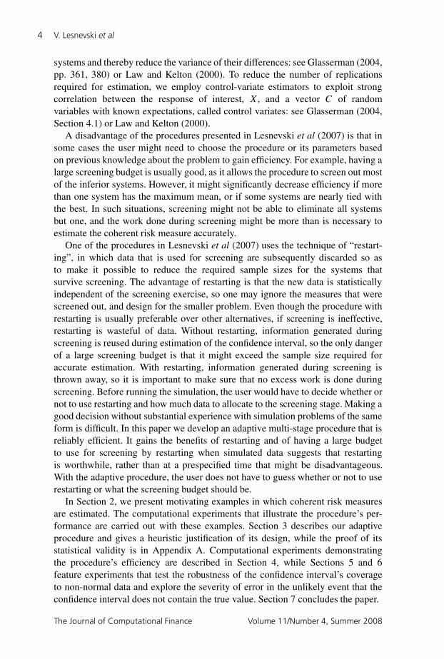
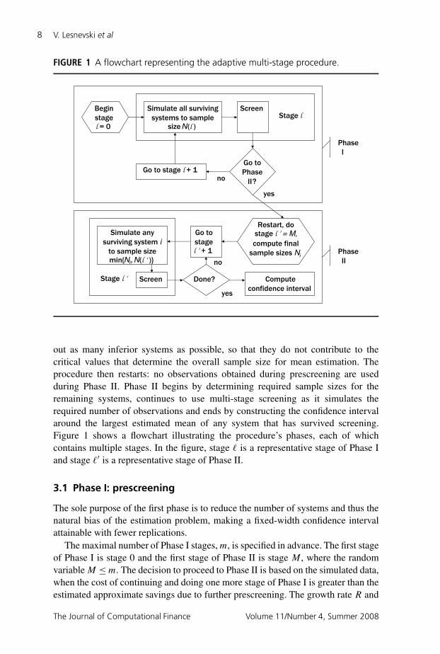
FIGURE 1 A flowchart representing the adaptive multi-stage procedure.

Go to stage l + 1

Simulate all surviving

systems to sample size N(l )

Begin

stagel = 0

Screen

Go to

Phase

?no

Phase

I

yes

Restart, dostage l ’ = M,

compute final

sample sizes Ni

Compute

confidence interval

Simulate any

surviving system i

to sample size min{Ni, N(l ‘ )}

Go to

stagel ’ + 1

Screen Done?Stage l ‘

Phase

II

yes

no

Stage l

II

out as many inferior systems as possible, so that they do not contribute to thecritical values that determine the overall sample size for mean estimation. Theprocedure then restarts: no observations obtained during prescreening are usedduring Phase II. Phase II begins by determining required sample sizes for theremaining systems, continues to use multi-stage screening as it simulates therequired number of observations and ends by constructing the confidence intervalaround the largest estimated mean of any system that has survived screening.Figure 1 shows a flowchart illustrating the procedure’s phases, each of whichcontains multiple stages. In the figure, stage is a representative stage of Phase Iand stage ′ is a representative stage of Phase II.

3.1 Phase I: prescreening

The sole purpose of the first phase is to reduce the number of systems and thus thenatural bias of the estimation problem, making a fixed-width confidence intervalattainable with fewer replications.

The maximal number of Phase I stages, m, is specified in advance. The first stageof Phase I is stage 0 and the first stage of Phase II is stage M , where the randomvariable M ≤m. The decision to proceed to Phase II is based on the simulated data,when the cost of continuing and doing one more stage of Phase I is greater than theestimated approximate savings due to further prescreening. The growth rate R and



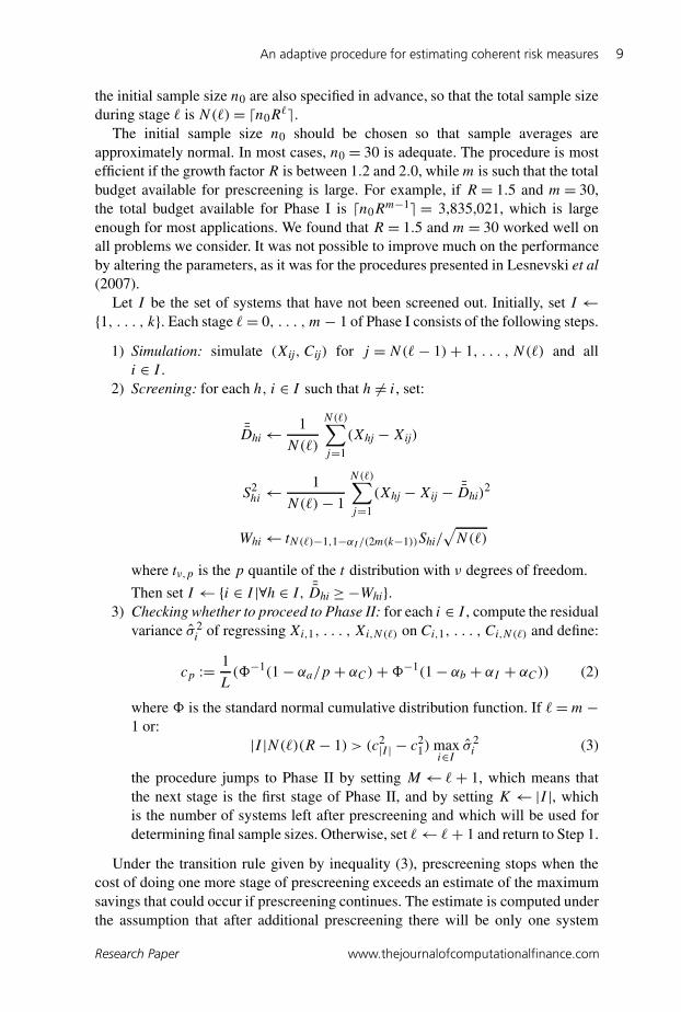
the initial sample size n0 are also specified in advance, so that the total sample sizeduring stage is N()= �n0R

�.The initial sample size n0 should be chosen so that sample averages are

approximately normal. In most cases, n0 = 30 is adequate. The procedure is mostefficient if the growth factor R is between 1.2 and 2.0, while m is such that the totalbudget available for prescreening is large. For example, if R = 1.5 and m= 30,the total budget available for Phase I is �n0R

m−1� = 3,835,021, which is largeenough for most applications. We found that R = 1.5 and m= 30 worked well onall problems we consider. It was not possible to improve much on the performanceby altering the parameters, as it was for the procedures presented in Lesnevski et al(2007).

Let I be the set of systems that have not been screened out. Initially, set I ←{1, . . . , k}. Each stage = 0, . . . , m− 1 of Phase I consists of the following steps.

1) Simulation: simulate (Xij, Cij) for j = N(− 1)+ 1, . . . , N() and alli ∈ I .

2) Screening: for each h, i ∈ I such that h = i, set:

¯Dhi← 1

N()

N()∑j=1

(Xhj − Xij)

S2hi←

1

N()− 1

N()∑j=1

(Xhj −Xij − ¯Dhi)2

Whi← tN()−1,1−αI /(2m(k−1))Shi/√

N()

where tν,p is the p quantile of the t distribution with ν degrees of freedom.

Then set I ← {i ∈ I |∀h ∈ I, ¯Dhi ≥−Whi}.3) Checking whether to proceed to Phase II: for each i ∈ I , compute the residual

variance σ 2i of regressing Xi,1, . . . , Xi,N() on Ci,1, . . . , Ci,N() and define:

cp := 1

L(�−1(1− αa/p + αC)+�−1(1− αb + αI + αC)) (2)

where � is the standard normal cumulative distribution function. If =m−1 or:

|I |N()(R − 1) > (c2|I | − c21) max

i∈I σ 2i (3)

the procedure jumps to Phase II by setting M← + 1, which means thatthe next stage is the first stage of Phase II, and by setting K← |I |, whichis the number of systems left after prescreening and which will be used fordetermining final sample sizes. Otherwise, set ← + 1 and return to Step 1.

Under the transition rule given by inequality (3), prescreening stops when thecost of doing one more stage of prescreening exceeds an estimate of the maximumsavings that could occur if prescreening continues. The estimate is computed underthe assumption that after additional prescreening there will be only one system



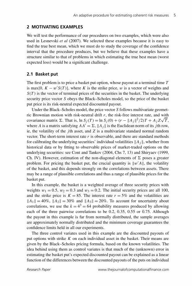
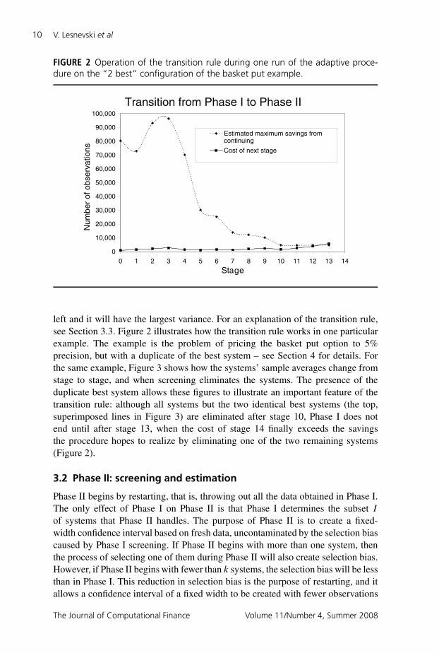
FIGURE 2 Operation of the transition rule during one run of the adaptive proce-dure on the “2 best” configuration of the basket put example.

Transition from Phase I to Phase II

0

10,000

20,000

30,000

40,000

50,000

60,000

70,000

80,000

90,000

100,000

0 1 2 3 4 5 6 7 8 9 10 11 12 13 14

Stage

continuingEstimated maximum savings from

Cost of next stage

Num

ber

of o

bser

vatio

ns

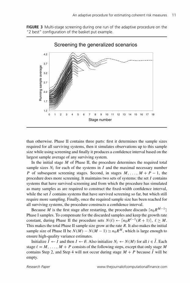
left and it will have the largest variance. For an explanation of the transition rule,see Section 3.3. Figure 2 illustrates how the transition rule works in one particularexample. The example is the problem of pricing the basket put option to 5%precision, but with a duplicate of the best system – see Section 4 for details. Forthe same example, Figure 3 shows how the systems’ sample averages change fromstage to stage, and when screening eliminates the systems. The presence of theduplicate best system allows these figures to illustrate an important feature of thetransition rule: although all systems but the two identical best systems (the top,superimposed lines in Figure 3) are eliminated after stage 10, Phase I does notend until after stage 13, when the cost of stage 14 finally exceeds the savingsthe procedure hopes to realize by eliminating one of the two remaining systems(Figure 2).

3.2 Phase II: screening and estimation

Phase II begins by restarting, that is, throwing out all the data obtained in Phase I.The only effect of Phase I on Phase II is that Phase I determines the subset I

of systems that Phase II handles. The purpose of Phase II is to create a fixed-width confidence interval based on fresh data, uncontaminated by the selection biascaused by Phase I screening. If Phase II begins with more than one system, thenthe process of selecting one of them during Phase II will also create selection bias.However, if Phase II begins with fewer than k systems, the selection bias will be lessthan in Phase I. This reduction in selection bias is the purpose of restarting, and itallows a confidence interval of a fixed width to be created with fewer observations



FIGURE 3 Multi-stage screening during one run of the adaptive procedure on the“2 best” configuration of the basket put example.

Screening the generalized scenarios

1.2

1.7

2.2

2.7

3.2

3.7

4.2

0 1 2 3 4 5 6 7 8 9 10 11 12 13 14 15 16 17 18

Stage number

Run

ning

sam

ple

aver

age

than otherwise. Phase II contains three parts: first it determines the sample sizesrequired for all surviving systems, then it simulates observations up to this samplesize while using screening and finally it produces a confidence interval based on thelargest sample average of any surviving system.

In the initial stage M of Phase II, the procedure determines the required totalsample sizes Ni for each of the systems in I and the maximal necessary numberP of subsequent screening stages. Second, in stages M, . . . , M + P − 1, theprocedure does more screening. It maintains two sets of systems: the set I containssystems that have survived screening and from which the procedure has simulatedas many samples as are required to construct the fixed-width confidence interval,while the set I contains systems that have survived screening so far, but which stillrequire more sampling. Finally, once the required sample size has been reached forall surviving systems, the procedure constructs a confidence interval.

Because M is the first stage after restarting, the procedure discards �n0RM−1�

Phase I samples. To compensate for the discarded samples and keep the growth rateconstant, during Phase II the procedure sets N()←�n0R

−1(R + 1)�, ≥M .This makes the total Phase II sample size grow at the rate R. It also makes the initialsample size of Phase II be N(M)−N(M − 1)� n0R

M , which is large enough toensure high-quality variance estimates.

Initialize I ← I and then I ←∅. Also initialize Ni←N(M) for all i ∈ I . Eachstage =M, . . . , M + P consists of the following steps, except that only stage M

contains Step 2, and Step 4 will not occur during stage M + P because I will beempty.



1) Simulation: simulate (Xij, Cij) for j = N(− 1)+ 1, . . . , min{Ni, N()}and all i ∈ I .Set n←N()−N(M − 1).

2) Setting final sample sizes: if > M , skip this step.Set α′′a ← αa/K − αC and α′′b ← αb − αI − αC , and set the scaling constant:

c← 1

L(tn−q−1,1−α′′a + tn−q−1,1−α′′b ) (4)

where q :=maxi∈I qi and each qi is the number of control variates in Ci .For each i ∈ I , compute the residual variance σ 2

i of regressingXi,N(M−1)+1, . . . , Xi,N(M) on Ci,N(M−1)+1, . . . , Ci,N(M), and from it thetotal sample size:

Ni←�c2σ 2i + χ2

qi ,1−αC� + N(M − 1) (5)

where χ2ν,p is the p quantile of the chi-squared distribution with ν degrees of

freedom.Set P ←�logR maxi∈I (Ni/N(M))�.

3) Updating I and I : add systems that have reached their required sample sizesto I and remove them from I : set I ← I ∪ {i ∈ I |Ni ≤N()} and I ← I\I .

4) Screening: for each h, i ∈ I such that h = i, set:

¯Dhi← 1

n

N()∑j=N(M−1)+1

(Xhj −Xij)

S2hi←

1

n− 1

N()∑j=N(M−1)+1

(Xhj −Xij − ¯Dhi)2

Whi← tn−1,1−αI /(2P (K−1))Shi/√

n

Then set I ←{i ∈ I |∀h ∈ I, ¯Dhi ≥−Whi}.5) Continue or compute confidence interval: if I = ∅, set ← + 1 and return

to Step 1.Otherwise, for each i ∈ I , compute the estimate µi from the regression ofXi,N(M−1)+1, . . . , Xi,Ni

on Ci,N(M−1)+1, . . . , Ci,Ni. Set:

a← 1

ctN(M)−N(M−1)−q−1,1−α′′a and

b← 1

ctN(M)−N(M−1)−q−1,1−α′′b

The confidence interval is:(maxi∈I µi − a, max

i∈I µi + b)



3.3 Efficiency of the rule for restarting

The adaptive procedure offers two significant improvements over our previousprocedures.

First, we do not need to specify a screening budget in advance. Choosingthe screening budget too small or too big could have a very significant effecton the performance of our previous procedures, in some configurations makinga simulation dozens of times slower; see Table 6 in Section 4.1. The adaptiveprocedure solves this problem by trying to screen out a system in Phase II onlyuntil its required sample size is reached. In effect, this allows the screening budgetto be arbitrarily large, to vary by system and to be determined adaptively by therequired sample size.

Second, the adaptive procedure allows us to restart whatever the configurationof the means µ1, . . . , µk may be. The effect of the decision whether or not torestart on performance is much less severe; as we will show below, usually we donot expect to save more than 40–80%. Restarting is usually beneficial because in atypical case there is only one best system. Having an adaptive prescreening phaseidentifying a good time to restart allows us to achieve very good performance in atypical case and reasonably good performance in all other cases.

How big are the benefits of prescreening in a typical case? To answer thisquestion let us first estimate the maximal possible savings due to restarting.

In the following analysis we make several simplifying assumptions. First,we assume that the estimate of the residual variance σ 2

i of system i is alwaysapproximately equal to the true residual variance σ 2

i . Second, we ignore the effectof the number of degrees of freedom on the sample sizes for estimation. Third,we assume that the effort required for screening out an inferior system is alwaysthe same, whether in Phase I, Phase II or in an alternative procedure withoutprescreening and restarting (such as the multi-stage procedure with early stoppingin Lesnevski et al (2007)).

The total cost E of a simulation without prescreening is the sum of the cost Es

of screening out inferior systems and the cost Ee of estimation of the survivingsystems: E = Es + Ee.

The total cost E of a simulation with prescreening is the sum of the prescreeningcost Ep, the cost Es of screening out inferior systems in Phase II and the estimationcost Ee of the surviving systems: E = Ep + Es + Ee.

Under our assumptions, the sample size Ni in Equation (5) is approximatelyequal to c2σ 2

i . Without prescreening, the constant c in Equation (4) is approxi-mately equal to ck defined in Equation (2), where k is the initial number of systems.With prescreening, c is approximately cK , where K is the number of systemsremaining after prescreening. The smaller K , the larger the benefit of prescreening,because smaller cK leads to smaller sample sizes for estimation.

We will assume that, whether we simulate with prescreening or not, the set I

of the surviving systems is the same. This is generally so when prescreening isstopped before the sample sizes for some systems exceed the sample sizes requiredfor estimation, which is exactly the case when prescreening could be beneficial.



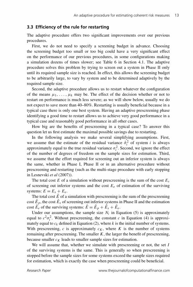
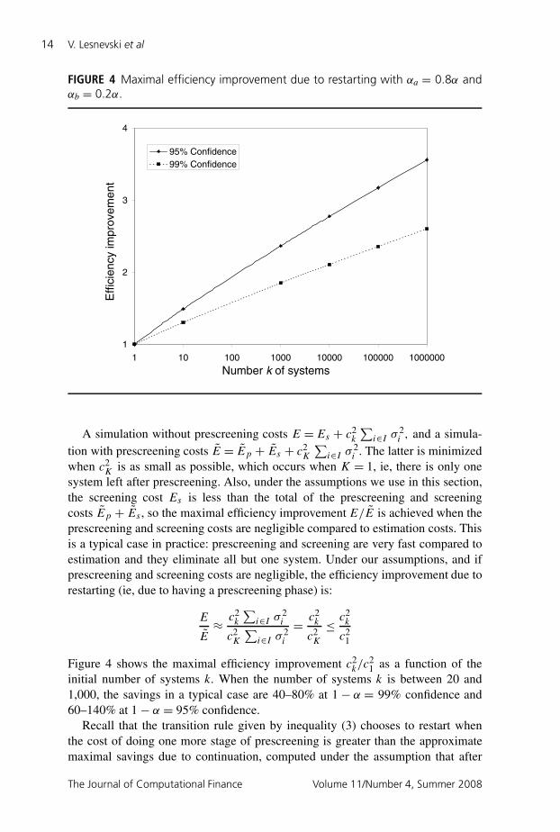
FIGURE 4 Maximal efficiency improvement due to restarting with αa = 0.8α andαb = 0.2α.

1

2

3

4

1 10 100 1000 10000 100000 1000000

Number k of systems

Effi

cien

cy im

prov

emen

t

95% Confidence99% Confidence

A simulation without prescreening costs E = Es + c2k

∑i∈I σ 2

i , and a simula-tion with prescreening costs E = Ep + Es + c2

K

∑i∈I σ 2

i . The latter is minimizedwhen c2

K is as small as possible, which occurs when K = 1, ie, there is only onesystem left after prescreening. Also, under the assumptions we use in this section,the screening cost Es is less than the total of the prescreening and screeningcosts Ep + Es , so the maximal efficiency improvement E/E is achieved when theprescreening and screening costs are negligible compared to estimation costs. Thisis a typical case in practice: prescreening and screening are very fast compared toestimation and they eliminate all but one system. Under our assumptions, and ifprescreening and screening costs are negligible, the efficiency improvement due torestarting (ie, due to having a prescreening phase) is:

E

E≈ c2

k

∑i∈I σ 2

i

c2K

∑i∈I σ 2

i

= c2k

c2K

≤ c2k

c21

Figure 4 shows the maximal efficiency improvement c2k/c

21 as a function of the

initial number of systems k. When the number of systems k is between 20 and1,000, the savings in a typical case are 40–80% at 1− α = 99% confidence and60–140% at 1− α = 95% confidence.

Recall that the transition rule given by inequality (3) chooses to restart whenthe cost of doing one more stage of prescreening is greater than the approximatemaximal savings due to continuation, computed under the assumption that after



additional prescreening there will be only one system left and it will have the largestvariance. A typical case indeed has one clear best system, so the effort required forscreening out inferior systems is relatively small, the approximate maximal savingsare relatively large and prescreening makes I a singleton.

How efficient is this transition rule in other situations? Let us consider aconfiguration when there are several systems that are tied for the best, while othersystems are relatively easy to screen out. In this case we might worry that the cost ofprescreening could get too high before the adaptive procedure proceeds to Phase II.Is our transition rule still efficient?

Because now we are concerned that prescreening may be too expensive, weassume that prescreening lasts a long time and eliminates all inferior systems: theset I (M) of systems used in Phase II equals I , the set of systems that survivescreening and reach their required sample sizes, and the Phase II cost of screeningEs = 0. Again we assume that I is the same whether we use prescreening or not:here we assume it contains only the systems that are tied. We now show how thetransition rule in inequality (3) provides a bound on Ep − Es , the excess cost ofprescreening in the adaptive procedure over the cost of screening in a procedurewithout restarting. The effort required to screen out inferior systems is similarin either procedure, so Ep − Es ≈KN(M − 1), the number of samples from theK = |I | surviving systems that the adaptive procedure throws out by restarting.

Prescreening stops after stage =M − 1, the first time that the cost (R − 1)

|I (+ 1)|N() of the next stage exceeds (c2|I (+1)| − c21) maxi∈I (+1) σ 2

i (). Underour present assumption that the residual variance estimates are approximatelycorrect, this yields the approximate upper bound:

N(M − 2)≤ (c2|I (M−1)| − c21) maxi∈I (M−1) σ 2

i

(R − 1)|I (M − 1)|

≤ (c2K − c2

1) maxi∈I σ 2i

(R − 1)K

because I (M − 1) contains I (M)= I whose size is K , and c2p defined in Equa-

tion (2) increases in p at a rate that is less than linear. Thus:

KN(M − 1)≤ KRN(M − 2)

≤ R(c2K − c2

1) maxi∈I σ 2i

R − 1

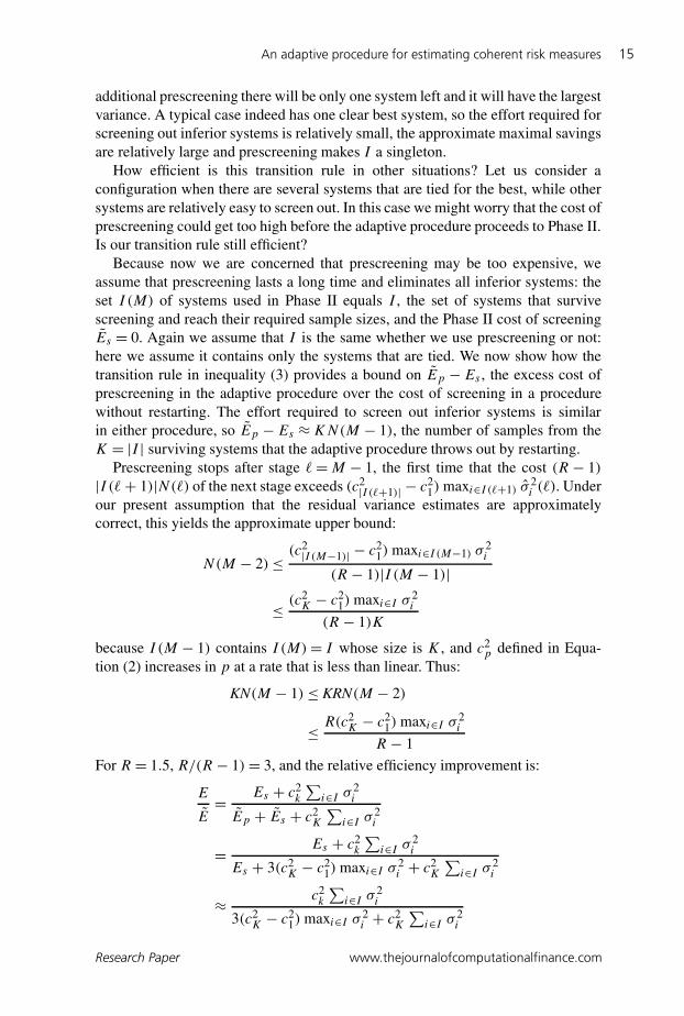
For R = 1.5, R/(R − 1)= 3, and the relative efficiency improvement is:

E

E= Es + c2

k

∑i∈I σ 2

i

Ep + Es + c2K

∑i∈I σ 2

i

= Es + c2k

∑i∈I σ 2

i

Es + 3(c2K − c2

1) maxi∈I σ 2i + c2

K

∑i∈I σ 2

i

≈ c2k

∑i∈I σ 2

i

3(c2K − c2

1) maxi∈I σ 2i + c2

K

∑i∈I σ 2

i



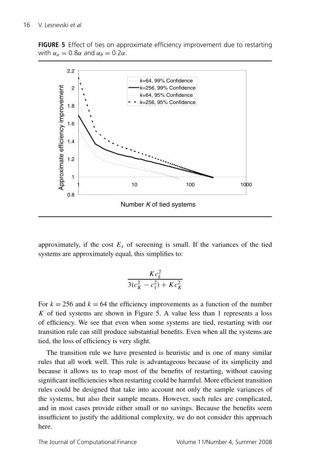
FIGURE 5 Effect of ties on approximate efficiency improvement due to restartingwith αa = 0.8α and αb = 0.2α.

0.8

1

1.2

1.4

1.6

1.8

2

2.2

1 10 100 1000

Number K of tied systems

App

roxi

mat

e ef

ficie

ncy

impr

ovem

ent

k=64, 99% Confidencek=256, 99% Confidencek=64, 95% Confidencek=256, 95% Confidence

approximately, if the cost Es of screening is small. If the variances of the tiedsystems are approximately equal, this simplifies to:

Kc2k

3(c2K − c2

1)+Kc2K

For k = 256 and k = 64 the efficiency improvements as a function of the numberK of tied systems are shown in Figure 5. A value less than 1 represents a lossof efficiency. We see that even when some systems are tied, restarting with ourtransition rule can still produce substantial benefits. Even when all the systems aretied, the loss of efficiency is very slight.

The transition rule we have presented is heuristic and is one of many similarrules that all work well. This rule is advantageous because of its simplicity andbecause it allows us to reap most of the benefits of restarting, without causingsignificant inefficiencies when restarting could be harmful. More efficient transitionrules could be designed that take into account not only the sample variances ofthe systems, but also their sample means. However, such rules are complicated,and in most cases provide either small or no savings. Because the benefits seeminsufficient to justify the additional complexity, we do not consider this approachhere.



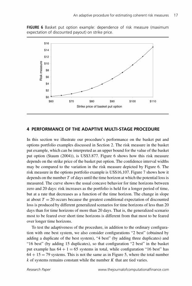
FIGURE 6 Basket put option example: dependence of risk measure (maximumexpectation of discounted payout) on strike price.

$0

$2

$4

$6

$8

$10

$12

$14

$16

$60 $70 $80 $90 $100 $110

Strike price of basket put option

Ris

k m

easu

re

4 PERFORMANCE OF THE ADAPTIVE MULTI-STAGE PROCEDURE

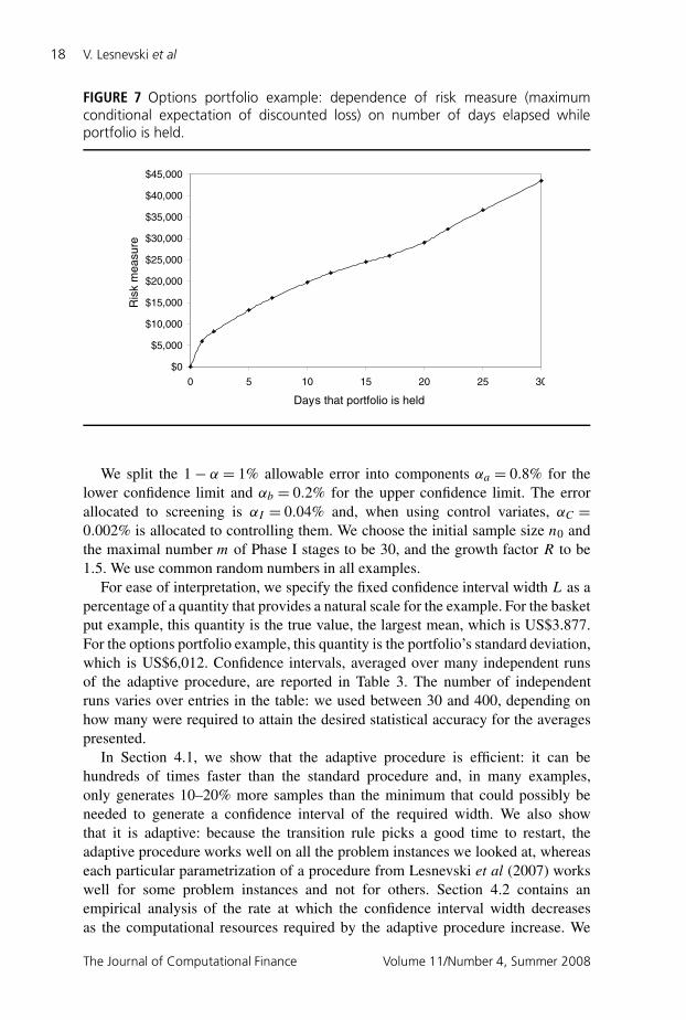
In this section we illustrate our procedure’s performance on the basket put andoptions portfolio examples discussed in Section 2. The risk measure in the basketput example, which can be interpreted as an upper bound for the value of the basketput option (Staum (2004)), is US$3.877. Figure 6 shows how this risk measuredepends on the strike price of the basket put option. The confidence interval widthsmay be compared to the variation in the risk measure depicted by Figure 6. Therisk measure in the options portfolio example is US$16,107. Figure 7 shows how itdepends on the number T of days until the time horizon at which the potential loss ismeasured. The curve shows the usual concave behavior for time horizons betweenzero and 20 days: risk increases as the portfolio is held for a longer period of time,but at a rate that decreases as a function of the time horizon. The change in slopeat about T = 20 occurs because the greatest conditional expectation of discountedloss is produced by different generalized scenarios for time horizons of less than 20days than for time horizons of more than 20 days. That is, the generalized scenariomost to be feared over short time horizons is different from that most to be fearedover longer time horizons.

To test the adaptiveness of the procedure, in addition to the ordinary configura-tion with one best system, we also consider configurations “2 best” (obtained byadding a duplicate of the best system), “4 best” (by adding three duplicates) and“16 best” (by adding 15 duplicates), so that configuration “2 best” in the basketput example has 64+ 1= 65 systems in total, while configuration “16 best” has64+ 15= 79 systems. This is not the same as in Figure 5, where the total numberk of systems remains constant while the number K that are tied varies.



FIGURE 7 Options portfolio example: dependence of risk measure (maximumconditional expectation of discounted loss) on number of days elapsed whileportfolio is held.

$0

$5,000

$10,000

$15,000

$20,000

$25,000

$30,000

$35,000

$40,000

$45,000

0 5 10 15 20 25 30

Days that portfolio is held

Ris

k m

easu

re

We split the 1− α = 1% allowable error into components αa = 0.8% for thelower confidence limit and αb = 0.2% for the upper confidence limit. The errorallocated to screening is αI = 0.04% and, when using control variates, αC =0.002% is allocated to controlling them. We choose the initial sample size n0 andthe maximal number m of Phase I stages to be 30, and the growth factor R to be1.5. We use common random numbers in all examples.

For ease of interpretation, we specify the fixed confidence interval width L as apercentage of a quantity that provides a natural scale for the example. For the basketput example, this quantity is the true value, the largest mean, which is US$3.877.For the options portfolio example, this quantity is the portfolio’s standard deviation,which is US$6,012. Confidence intervals, averaged over many independent runsof the adaptive procedure, are reported in Table 3. The number of independentruns varies over entries in the table: we used between 30 and 400, depending onhow many were required to attain the desired statistical accuracy for the averagespresented.

In Section 4.1, we show that the adaptive procedure is efficient: it can behundreds of times faster than the standard procedure and, in many examples,only generates 10–20% more samples than the minimum that could possibly beneeded to generate a confidence interval of the required width. We also showthat it is adaptive: because the transition rule picks a good time to restart, theadaptive procedure works well on all the problem instances we looked at, whereaseach particular parametrization of a procedure from Lesnevski et al (2007) workswell for some problem instances and not for others. Section 4.2 contains anempirical analysis of the rate at which the confidence interval width decreasesas the computational resources required by the adaptive procedure increase. We



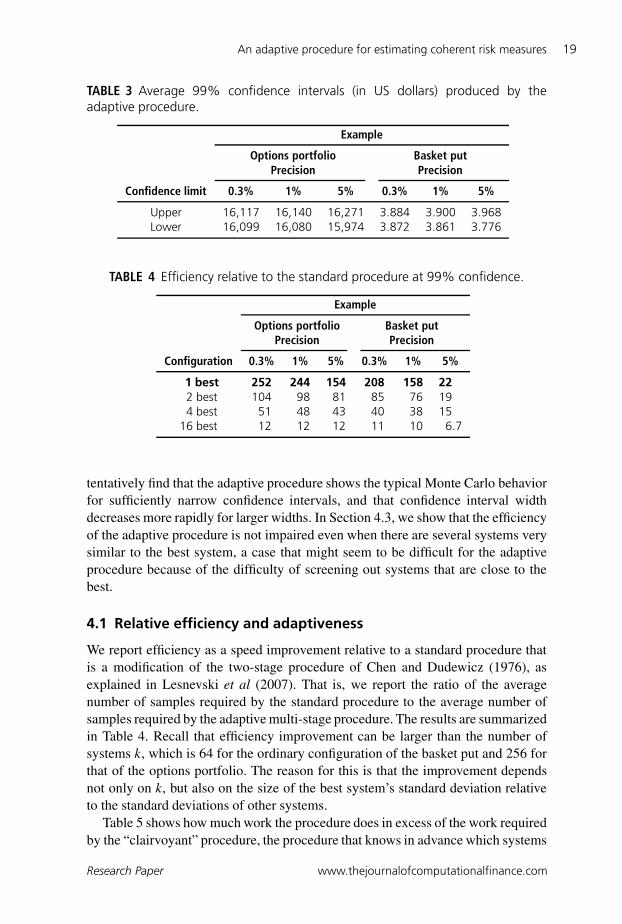
TABLE 3 Average 99% confidence intervals (in US dollars) produced by theadaptive procedure.

Example

Options portfolio Basket putPrecision Precision

Confidence limit 0.3% 1% 5% 0.3% 1% 5%

Upper 16,117 16,140 16,271 3.884 3.900 3.968Lower 16,099 16,080 15,974 3.872 3.861 3.776

TABLE 4 Efficiency relative to the standard procedure at 99% confidence.

Example


Configuration 0.3% 1% 5% 0.3% 1% 5%

1 best 252 244 154 208 158 222 best 104 98 81 85 76 194 best 51 48 43 40 38 15

16 best 12 12 12 11 10 6.7

tentatively find that the adaptive procedure shows the typical Monte Carlo behaviorfor sufficiently narrow confidence intervals, and that confidence interval widthdecreases more rapidly for larger widths. In Section 4.3, we show that the efficiencyof the adaptive procedure is not impaired even when there are several systems verysimilar to the best system, a case that might seem to be difficult for the adaptiveprocedure because of the difficulty of screening out systems that are close to thebest.

4.1 Relative efficiency and adaptiveness

We report efficiency as a speed improvement relative to a standard procedure thatis a modification of the two-stage procedure of Chen and Dudewicz (1976), asexplained in Lesnevski et al (2007). That is, we report the ratio of the averagenumber of samples required by the standard procedure to the average number ofsamples required by the adaptive multi-stage procedure. The results are summarizedin Table 4. Recall that efficiency improvement can be larger than the number ofsystems k, which is 64 for the ordinary configuration of the basket put and 256 forthat of the options portfolio. The reason for this is that the improvement dependsnot only on k, but also on the size of the best system’s standard deviation relativeto the standard deviations of other systems.

Table 5 shows how much work the procedure does in excess of the work requiredby the “clairvoyant” procedure, the procedure that knows in advance which systems



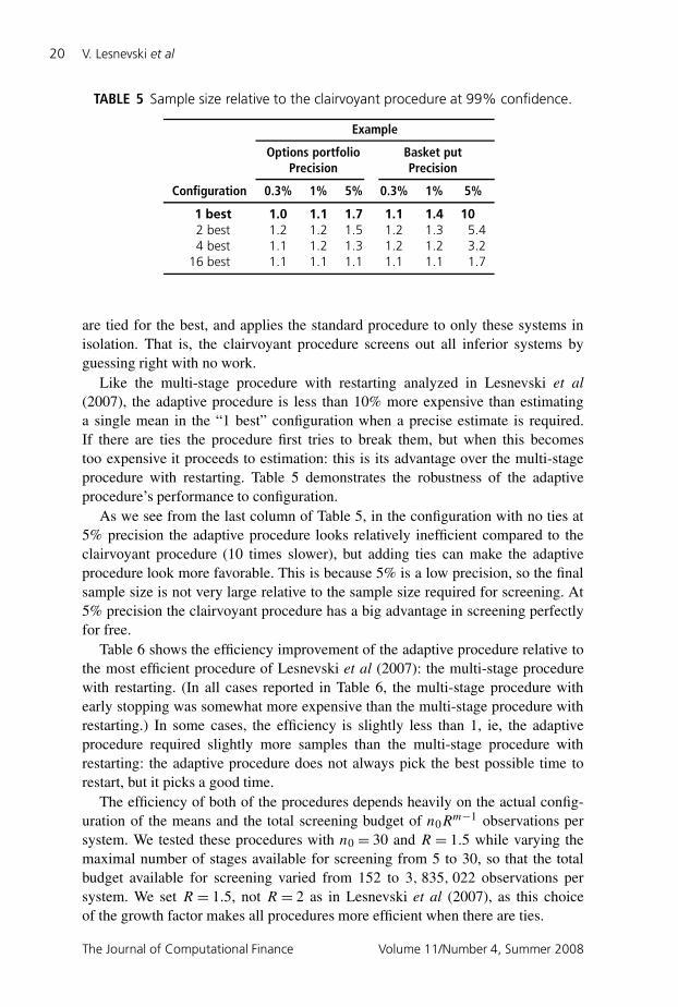
TABLE 5 Sample size relative to the clairvoyant procedure at 99% confidence.

Example


Configuration 0.3% 1% 5% 0.3% 1% 5%

1 best 1.0 1.1 1.7 1.1 1.4 102 best 1.2 1.2 1.5 1.2 1.3 5.44 best 1.1 1.2 1.3 1.2 1.2 3.2

16 best 1.1 1.1 1.1 1.1 1.1 1.7

are tied for the best, and applies the standard procedure to only these systems inisolation. That is, the clairvoyant procedure screens out all inferior systems byguessing right with no work.

Like the multi-stage procedure with restarting analyzed in Lesnevski et al(2007), the adaptive procedure is less than 10% more expensive than estimatinga single mean in the “1 best” configuration when a precise estimate is required.If there are ties the procedure first tries to break them, but when this becomestoo expensive it proceeds to estimation: this is its advantage over the multi-stageprocedure with restarting. Table 5 demonstrates the robustness of the adaptiveprocedure’s performance to configuration.

As we see from the last column of Table 5, in the configuration with no ties at5% precision the adaptive procedure looks relatively inefficient compared to theclairvoyant procedure (10 times slower), but adding ties can make the adaptiveprocedure look more favorable. This is because 5% is a low precision, so the finalsample size is not very large relative to the sample size required for screening. At5% precision the clairvoyant procedure has a big advantage in screening perfectlyfor free.

Table 6 shows the efficiency improvement of the adaptive procedure relative tothe most efficient procedure of Lesnevski et al (2007): the multi-stage procedurewith restarting. (In all cases reported in Table 6, the multi-stage procedure withearly stopping was somewhat more expensive than the multi-stage procedure withrestarting.) In some cases, the efficiency is slightly less than 1, ie, the adaptiveprocedure required slightly more samples than the multi-stage procedure withrestarting: the adaptive procedure does not always pick the best possible time torestart, but it picks a good time.

The efficiency of both of the procedures depends heavily on the actual config-uration of the means and the total screening budget of n0R

m−1 observations persystem. We tested these procedures with n0 = 30 and R = 1.5 while varying themaximal number of stages available for screening from 5 to 30, so that the totalbudget available for screening varied from 152 to 3, 835, 022 observations persystem. We set R = 1.5, not R = 2 as in Lesnevski et al (2007), as this choiceof the growth factor makes all procedures more efficient when there are ties.



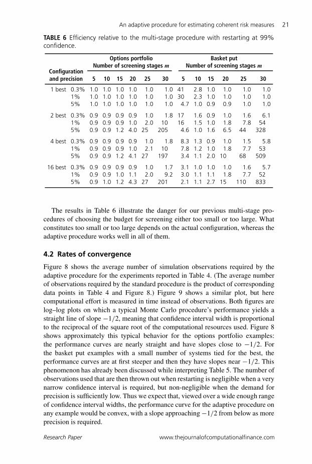
TABLE 6 Efficiency relative to the multi-stage procedure with restarting at 99%confidence.

Options portfolio Basket putNumber of screening stages m Number of screening stages m

Configurationand precision 5 10 15 20 25 30 5 10 15 20 25 30

1 best 0.3% 1.0 1.0 1.0 1.0 1.0 1.0 41 2.8 1.0 1.0 1.0 1.01% 1.0 1.0 1.0 1.0 1.0 1.0 30 2.3 1.0 1.0 1.0 1.05% 1.0 1.0 1.0 1.0 1.0 1.0 4.7 1.0 0.9 0.9 1.0 1.0

2 best 0.3% 0.9 0.9 0.9 0.9 1.0 1.8 17 1.6 0.9 1.0 1.6 6.11% 0.9 0.9 0.9 1.0 2.0 10 16 1.5 1.0 1.8 7.8 545% 0.9 0.9 1.2 4.0 25 205 4.6 1.0 1.6 6.5 44 328

4 best 0.3% 0.9 0.9 0.9 0.9 1.0 1.8 8.3 1.3 0.9 1.0 1.5 5.81% 0.9 0.9 0.9 1.0 2.1 10 7.8 1.2 1.0 1.8 7.7 535% 0.9 0.9 1.2 4.1 27 197 3.4 1.1 2.0 10 68 509

16 best 0.3% 0.9 0.9 0.9 0.9 1.0 1.7 3.1 1.0 1.0 1.0 1.6 5.71% 0.9 0.9 1.0 1.1 2.0 9.2 3.0 1.1 1.1 1.8 7.7 525% 0.9 1.0 1.2 4.3 27 201 2.1 1.1 2.7 15 110 833

The results in Table 6 illustrate the danger for our previous multi-stage pro-cedures of choosing the budget for screening either too small or too large. Whatconstitutes too small or too large depends on the actual configuration, whereas theadaptive procedure works well in all of them.

4.2 Rates of convergence

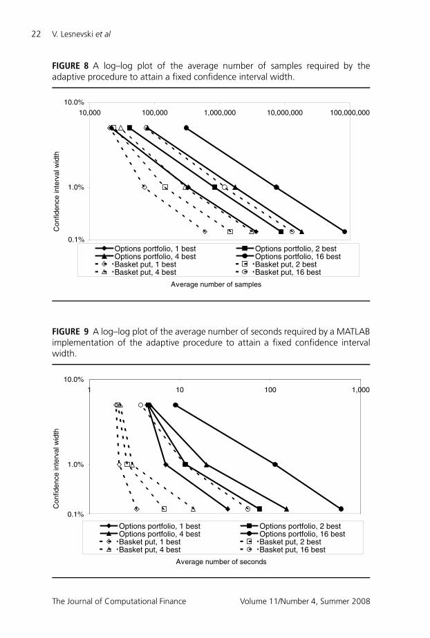
Figure 8 shows the average number of simulation observations required by theadaptive procedure for the experiments reported in Table 4. (The average numberof observations required by the standard procedure is the product of correspondingdata points in Table 4 and Figure 8.) Figure 9 shows a similar plot, but herecomputational effort is measured in time instead of observations. Both figures arelog–log plots on which a typical Monte Carlo procedure’s performance yields astraight line of slope −1/2, meaning that confidence interval width is proportionalto the reciprocal of the square root of the computational resources used. Figure 8shows approximately this typical behavior for the options portfolio examples:the performance curves are nearly straight and have slopes close to −1/2. Forthe basket put examples with a small number of systems tied for the best, theperformance curves are at first steeper and then they have slopes near −1/2. Thisphenomenon has already been discussed while interpreting Table 5. The number ofobservations used that are then thrown out when restarting is negligible when a verynarrow confidence interval is required, but non-negligible when the demand forprecision is sufficiently low. Thus we expect that, viewed over a wide enough rangeof confidence interval widths, the performance curve for the adaptive procedure onany example would be convex, with a slope approaching−1/2 from below as moreprecision is required.



FIGURE 8 A log–log plot of the average number of samples required by theadaptive procedure to attain a fixed confidence interval width.

0.1%

1.0%

10.0%

10,000 100,000 1,000,000 10,000,000 100,000,000

Average number of samples

Con

fiden

ce in

terv

al w

idth

Options portfolio, 1 best Options portfolio, 2 bestOptions portfolio, 4 best Options portfolio, 16 bestBasket put, 1 best Basket put, 2 bestBasket put, 4 best Basket put, 16 best

FIGURE 9 A log–log plot of the average number of seconds required by a MATLABimplementation of the adaptive procedure to attain a fixed confidence intervalwidth.

0.1%

1.0%

10.0%

1 10 100 1,000

Average number of seconds

Con

fiden

ce in

terv

al w

idth

Options portfolio, 1 best Options portfolio, 2 bestOptions portfolio, 4 best Options portfolio, 16 bestBasket put, 1 best Basket put, 2 bestBasket put, 4 best Basket put, 16 best



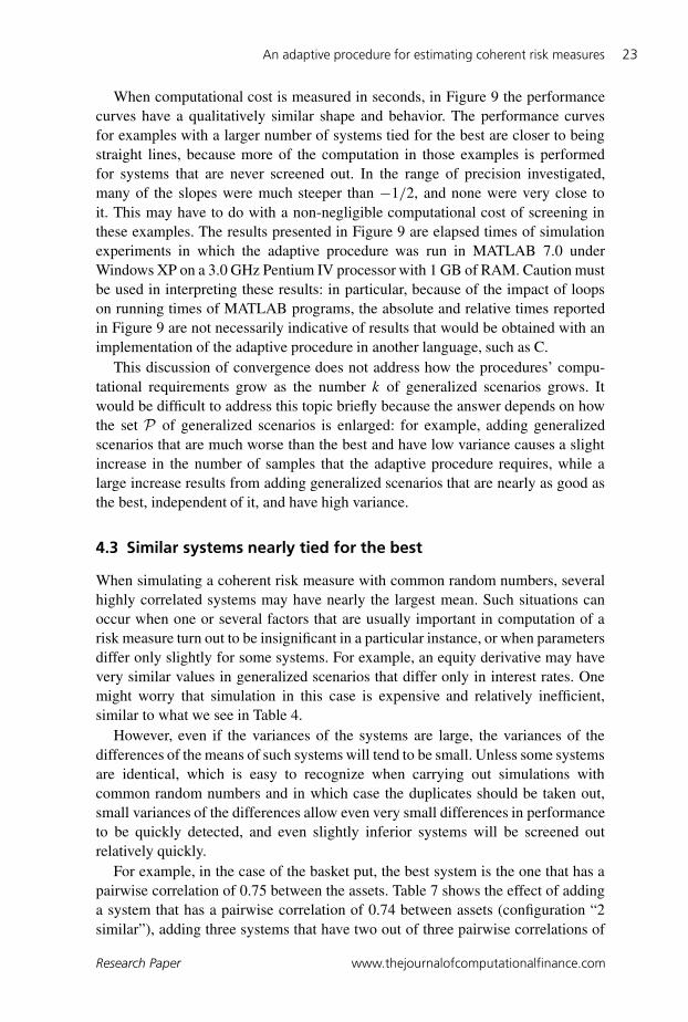
When computational cost is measured in seconds, in Figure 9 the performancecurves have a qualitatively similar shape and behavior. The performance curvesfor examples with a larger number of systems tied for the best are closer to beingstraight lines, because more of the computation in those examples is performedfor systems that are never screened out. In the range of precision investigated,many of the slopes were much steeper than −1/2, and none were very close toit. This may have to do with a non-negligible computational cost of screening inthese examples. The results presented in Figure 9 are elapsed times of simulationexperiments in which the adaptive procedure was run in MATLAB 7.0 underWindows XP on a 3.0 GHz Pentium IV processor with 1 GB of RAM. Caution mustbe used in interpreting these results: in particular, because of the impact of loopson running times of MATLAB programs, the absolute and relative times reportedin Figure 9 are not necessarily indicative of results that would be obtained with animplementation of the adaptive procedure in another language, such as C.

This discussion of convergence does not address how the procedures’ compu-tational requirements grow as the number k of generalized scenarios grows. Itwould be difficult to address this topic briefly because the answer depends on howthe set P of generalized scenarios is enlarged: for example, adding generalizedscenarios that are much worse than the best and have low variance causes a slightincrease in the number of samples that the adaptive procedure requires, while alarge increase results from adding generalized scenarios that are nearly as good asthe best, independent of it, and have high variance.

4.3 Similar systems nearly tied for the best

When simulating a coherent risk measure with common random numbers, severalhighly correlated systems may have nearly the largest mean. Such situations canoccur when one or several factors that are usually important in computation of arisk measure turn out to be insignificant in a particular instance, or when parametersdiffer only slightly for some systems. For example, an equity derivative may havevery similar values in generalized scenarios that differ only in interest rates. Onemight worry that simulation in this case is expensive and relatively inefficient,similar to what we see in Table 4.

However, even if the variances of the systems are large, the variances of thedifferences of the means of such systems will tend to be small. Unless some systemsare identical, which is easy to recognize when carrying out simulations withcommon random numbers and in which case the duplicates should be taken out,small variances of the differences allow even very small differences in performanceto be quickly detected, and even slightly inferior systems will be screened outrelatively quickly.

For example, in the case of the basket put, the best system is the one that has apairwise correlation of 0.75 between the assets. Table 7 shows the effect of addinga system that has a pairwise correlation of 0.74 between assets (configuration “2similar”), adding three systems that have two out of three pairwise correlations of



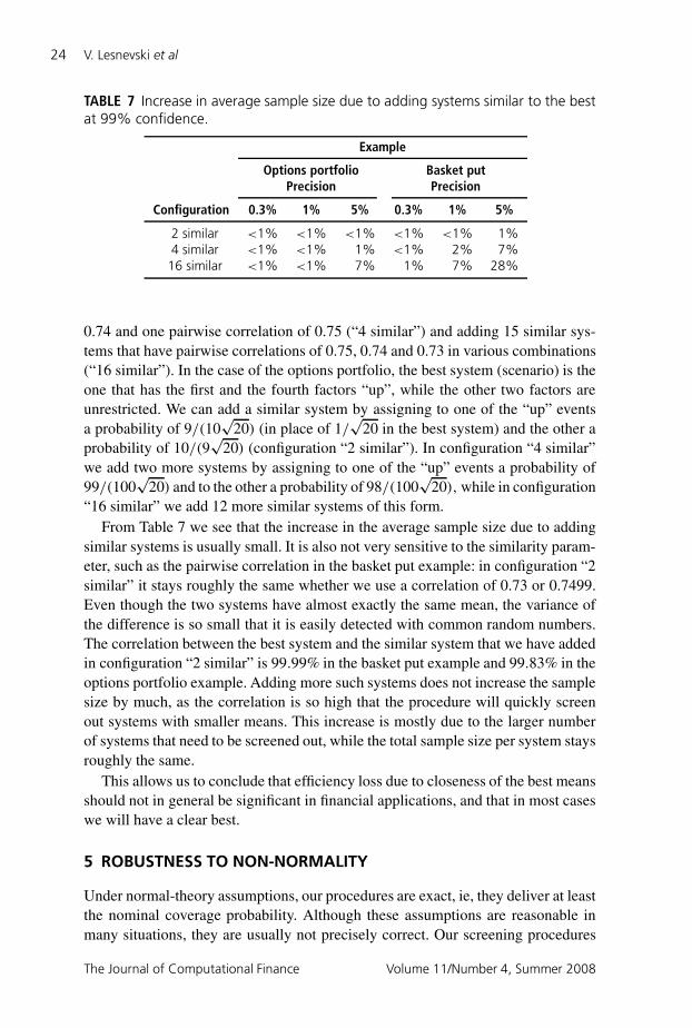
TABLE 7 Increase in average sample size due to adding systems similar to the bestat 99% confidence.

Example


Configuration 0.3% 1% 5% 0.3% 1% 5%

2 similar <1% <1% <1% <1% <1% 1%4 similar <1% <1% 1% <1% 2% 7%

16 similar <1% <1% 7% 1% 7% 28%

0.74 and one pairwise correlation of 0.75 (“4 similar”) and adding 15 similar sys-tems that have pairwise correlations of 0.75, 0.74 and 0.73 in various combinations(“16 similar”). In the case of the options portfolio, the best system (scenario) is theone that has the first and the fourth factors “up”, while the other two factors areunrestricted. We can add a similar system by assigning to one of the “up” eventsa probability of 9/(10

√20) (in place of 1/

√20 in the best system) and the other a

probability of 10/(9√

20) (configuration “2 similar”). In configuration “4 similar”we add two more systems by assigning to one of the “up” events a probability of99/(100

√20) and to the other a probability of 98/(100

√20), while in configuration

“16 similar” we add 12 more similar systems of this form.From Table 7 we see that the increase in the average sample size due to adding

similar systems is usually small. It is also not very sensitive to the similarity param-eter, such as the pairwise correlation in the basket put example: in configuration “2similar” it stays roughly the same whether we use a correlation of 0.73 or 0.7499.Even though the two systems have almost exactly the same mean, the variance ofthe difference is so small that it is easily detected with common random numbers.The correlation between the best system and the similar system that we have addedin configuration “2 similar” is 99.99% in the basket put example and 99.83% in theoptions portfolio example. Adding more such systems does not increase the samplesize by much, as the correlation is so high that the procedure will quickly screenout systems with smaller means. This increase is mostly due to the larger numberof systems that need to be screened out, while the total sample size per system staysroughly the same.

This allows us to conclude that efficiency loss due to closeness of the best meansshould not in general be significant in financial applications, and that in most caseswe will have a clear best.

5 ROBUSTNESS TO NON-NORMALITY

Under normal-theory assumptions, our procedures are exact, ie, they deliver at leastthe nominal coverage probability. Although these assumptions are reasonable inmany situations, they are usually not precisely correct. Our screening procedures



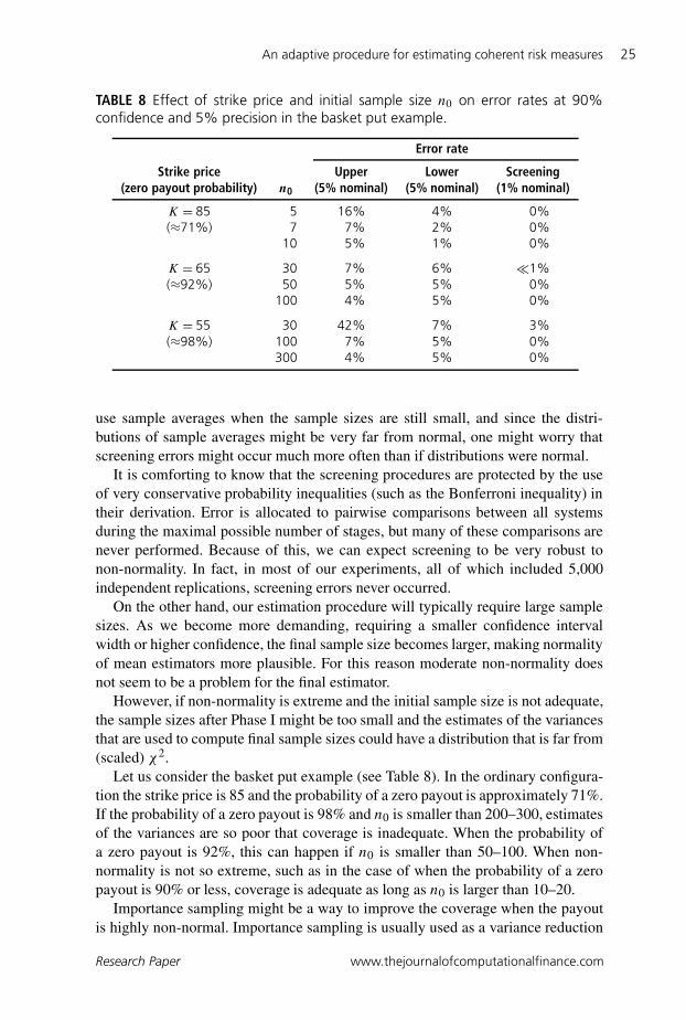
TABLE 8 Effect of strike price and initial sample size n0 on error rates at 90%confidence and 5% precision in the basket put example.

Error rate

Strike price Upper Lower Screening(zero payout probability) n0 (5% nominal) (5% nominal) (1% nominal)

K = 85 5 16% 4% 0%(≈71%) 7 7% 2% 0%

10 5% 1% 0%

K = 65 30 7% 6% �1%(≈92%) 50 5% 5% 0%

100 4% 5% 0%

K = 55 30 42% 7% 3%(≈98%) 100 7% 5% 0%

300 4% 5% 0%

use sample averages when the sample sizes are still small, and since the distri-butions of sample averages might be very far from normal, one might worry thatscreening errors might occur much more often than if distributions were normal.

It is comforting to know that the screening procedures are protected by the useof very conservative probability inequalities (such as the Bonferroni inequality) intheir derivation. Error is allocated to pairwise comparisons between all systemsduring the maximal possible number of stages, but many of these comparisons arenever performed. Because of this, we can expect screening to be very robust tonon-normality. In fact, in most of our experiments, all of which included 5,000independent replications, screening errors never occurred.

On the other hand, our estimation procedure will typically require large samplesizes. As we become more demanding, requiring a smaller confidence intervalwidth or higher confidence, the final sample size becomes larger, making normalityof mean estimators more plausible. For this reason moderate non-normality doesnot seem to be a problem for the final estimator.

However, if non-normality is extreme and the initial sample size is not adequate,the sample sizes after Phase I might be too small and the estimates of the variancesthat are used to compute final sample sizes could have a distribution that is far from(scaled) χ2.

Let us consider the basket put example (see Table 8). In the ordinary configura-tion the strike price is 85 and the probability of a zero payout is approximately 71%.If the probability of a zero payout is 98% and n0 is smaller than 200–300, estimatesof the variances are so poor that coverage is inadequate. When the probability ofa zero payout is 92%, this can happen if n0 is smaller than 50–100. When non-normality is not so extreme, such as in the case of when the probability of a zeropayout is 90% or less, coverage is adequate as long as n0 is larger than 10–20.

Importance sampling might be a way to improve the coverage when the payoutis highly non-normal. Importance sampling is usually used as a variance reduction



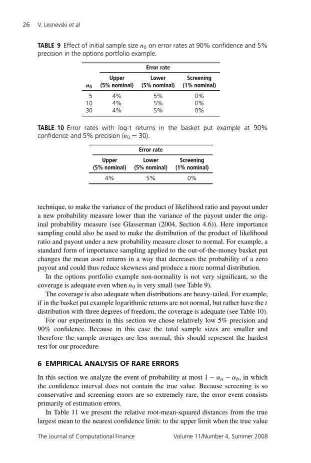
TABLE 9 Effect of initial sample size n0 on error rates at 90% confidence and 5%precision in the options portfolio example.

Error rate

Upper Lower Screeningn0 (5% nominal) (5% nominal) (1% nominal)

5 4% 5% 0%10 4% 5% 0%30 4% 5% 0%

TABLE 10 Error rates with log-t returns in the basket put example at 90%confidence and 5% precision (n0 = 30).

Error rate

Upper Lower Screening(5% nominal) (5% nominal) (1% nominal)

4% 5% 0%

technique, to make the variance of the product of likelihood ratio and payout undera new probability measure lower than the variance of the payout under the orig-inal probability measure (see Glasserman (2004, Section 4.6)). Here importancesampling could also be used to make the distribution of the product of likelihoodratio and payout under a new probability measure closer to normal. For example, astandard form of importance sampling applied to the out-of-the-money basket putchanges the mean asset returns in a way that decreases the probability of a zeropayout and could thus reduce skewness and produce a more normal distribution.

In the options portfolio example non-normality is not very significant, so thecoverage is adequate even when n0 is very small (see Table 9).

The coverage is also adequate when distributions are heavy-tailed. For example,if in the basket put example logarithmic returns are not normal, but rather have the t

distribution with three degrees of freedom, the coverage is adequate (see Table 10).For our experiments in this section we chose relatively low 5% precision and

90% confidence. Because in this case the total sample sizes are smaller andtherefore the sample averages are less normal, this should represent the hardesttest for our procedure.

6 EMPIRICAL ANALYSIS OF RARE ERRORS

In this section we analyze the event of probability at most 1− αa − αb, in whichthe confidence interval does not contain the true value. Because screening is soconservative and screening errors are so extremely rare, the error event consistsprimarily of estimation errors.

In Table 11 we present the relative root-mean-squared distances from the truelargest mean to the nearest confidence limit: to the upper limit when the true value



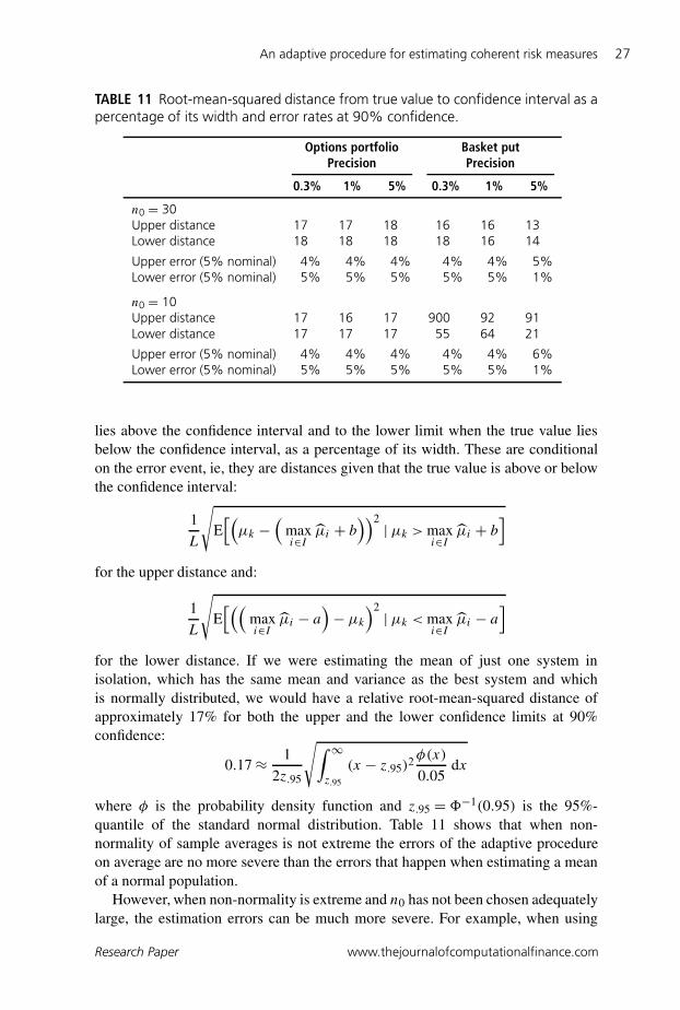
TABLE 11 Root-mean-squared distance from true value to confidence interval as apercentage of its width and error rates at 90% confidence.


0.3% 1% 5% 0.3% 1% 5%

n0 = 30Upper distance 17 17 18 16 16 13Lower distance 18 18 18 18 16 14

Upper error (5% nominal) 4% 4% 4% 4% 4% 5%Lower error (5% nominal) 5% 5% 5% 5% 5% 1%

n0 = 10Upper distance 17 16 17 900 92 91Lower distance 17 17 17 55 64 21

Upper error (5% nominal) 4% 4% 4% 4% 4% 6%Lower error (5% nominal) 5% 5% 5% 5% 5% 1%

lies above the confidence interval and to the lower limit when the true value liesbelow the confidence interval, as a percentage of its width. These are conditionalon the error event, ie, they are distances given that the true value is above or belowthe confidence interval:

1

L

√E[(

µk −(

maxi∈I µi + b

))2 | µk > maxi∈I µi + b

]for the upper distance and:

1

L

√E[((

maxi∈I µi − a

)− µk

)2 | µk < maxi∈I µi − a

]for the lower distance. If we were estimating the mean of just one system inisolation, which has the same mean and variance as the best system and whichis normally distributed, we would have a relative root-mean-squared distance ofapproximately 17% for both the upper and the lower confidence limits at 90%confidence:

0.17≈ 1

2z.95

√∫ ∞z.95

(x − z.95)2 φ(x)

0.05dx

where φ is the probability density function and z.95 =�−1(0.95) is the 95%-quantile of the standard normal distribution. Table 11 shows that when non-normality of sample averages is not extreme the errors of the adaptive procedureon average are no more severe than the errors that happen when estimating a meanof a normal population.

However, when non-normality is extreme and n0 has not been chosen adequatelylarge, the estimation errors can be much more severe. For example, when using



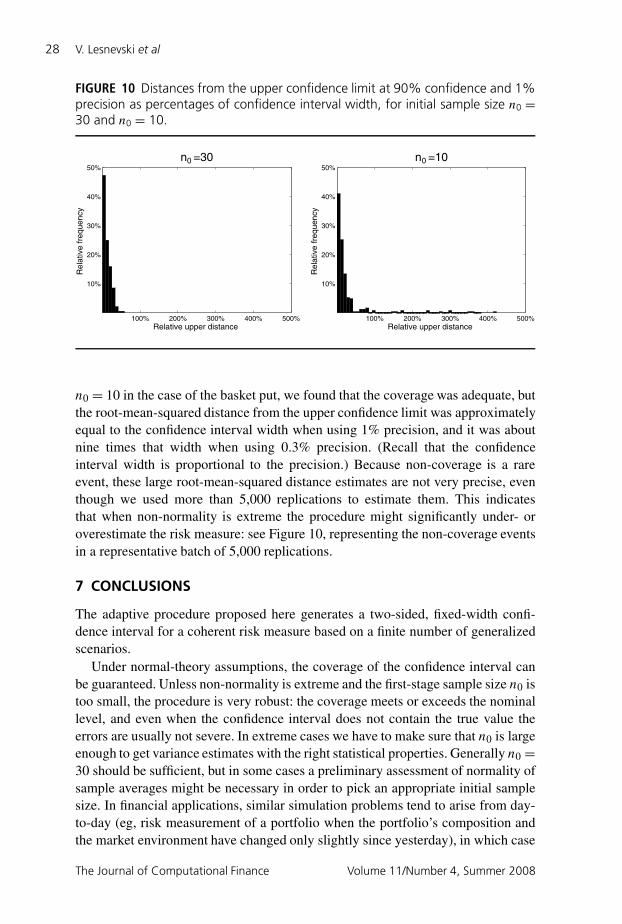
FIGURE 10 Distances from the upper confidence limit at 90% confidence and 1%precision as percentages of confidence interval width, for initial sample size n0 =30 and n0 = 10.

100% 200% 300% 400% 500%

10%

20%

30%

40%

50%

Relative upper distance

Rel

ativ

e fr

eque

ncy

100% 200% 300% 400% 500%

10%

20%

30%

40%

50%

Relative upper distance

Rel

ativ

e fr

eque

ncy

n0 =30 n0 =10

n0 = 10 in the case of the basket put, we found that the coverage was adequate, butthe root-mean-squared distance from the upper confidence limit was approximatelyequal to the confidence interval width when using 1% precision, and it was aboutnine times that width when using 0.3% precision. (Recall that the confidenceinterval width is proportional to the precision.) Because non-coverage is a rareevent, these large root-mean-squared distance estimates are not very precise, eventhough we used more than 5,000 replications to estimate them. This indicatesthat when non-normality is extreme the procedure might significantly under- oroverestimate the risk measure: see Figure 10, representing the non-coverage eventsin a representative batch of 5,000 replications.

7 CONCLUSIONS

The adaptive procedure proposed here generates a two-sided, fixed-width confi-dence interval for a coherent risk measure based on a finite number of generalizedscenarios.

Under normal-theory assumptions, the coverage of the confidence interval canbe guaranteed. Unless non-normality is extreme and the first-stage sample size n0 istoo small, the procedure is very robust: the coverage meets or exceeds the nominallevel, and even when the confidence interval does not contain the true value theerrors are usually not severe. In extreme cases we have to make sure that n0 is largeenough to get variance estimates with the right statistical properties. Generally n0 =30 should be sufficient, but in some cases a preliminary assessment of normality ofsample averages might be necessary in order to pick an appropriate initial samplesize. In financial applications, similar simulation problems tend to arise from day-to-day (eg, risk measurement of a portfolio when the portfolio’s composition andthe market environment have changed only slightly since yesterday), in which case



extra simulation effort would not be required to determine an appropriate valueof n0. The problems due to non-normality can also be mitigated by importancesampling. It might also be possible to improve robustness to non-normality bychanging the screening procedure. We have carried out screening on the basis ofa two-sample t test with paired observations. Screening could also be carried outbased on a non-parametric test. One relevant approach is the nonparametric subsetselection procedure of Hsu (1980).

The adaptive procedure improves upon previous procedures, which mightdecrease efficiency when applied to the wrong problem or with the wrong parame-ters, by being more reliably efficient and easier to use. One might fear that the timerequired to estimate a coherent risk measure based on k generalized scenarios wouldbe of the order of k times as long as the time required to estimate a single mean,and this is true for standard methods. The adaptive procedure is typically dozensto hundreds of times faster than standard methods for k = 64 or k = 256, even forchallenging problems in which some of the generalized scenario means are verysimilar or even tied. Even for these challenging problems, the adaptive procedurewas only a few percent to 40% more expensive than estimating a single mean forthe examples we investigated of generating a moderately precise 99% confidenceinterval for a coherent risk measure (Tables 5 and 7, precision 1% or less).

It seems difficult, then, to construct a procedure that is much more efficientfor these problems while providing a valid confidence interval. However, it maybe possible to improve efficiency for problems where a wide confidence intervalis acceptable. We tried using fully sequential screening instead of multi-stagescreening, but found that this seldom improved efficiency. Another possibility isto avoid using the conservative probability inequalities we used to guarantee theconfidence interval’s coverage probability. Pursuing this line of thought, one mightalso develop a procedure that provides only a point estimate for the risk measure andnot a confidence interval: it may be possible to get a point estimator of comparablequality faster than our confidence interval by screening more aggressively thanour probability inequalities permit or by avoiding restarting. Furthermore, forapplications that require a point estimator, it could be valuable to apply bias-reduction techniques to get a point estimator superior to the straightforward one,which is the maximum surviving sample average maxi∈I µi around which ourconfidence interval is constructed.

APPENDIX A VALIDITY OF THE PROCEDURE

While I is the set of systems that survives screening after Phase II, let [k] be theindex of the best system, the one with the largest mean. Let I (M) be the set ofsystems that survives screening in Phase I, and let [k]M be the best system in I (M).

PROPOSITION A.1 If, for each i = 1, 2, . . . , k, Xij = µi + (Cij − ξi)′βi + ηij,

where the residuals {ηij, j = 1, 2, . . .} and controls {Cij , j = 1, 2, . . .} are inde-pendent sets of independently and identically distributed normal random variables,βi is an unknown constant vector, E[Ci1] = ξi and E[ηi1] = 0, then the procedure



satisfies:

Pr{µ[k] ≥max

i∈I µi − a}≥ 1− αa (A.1)

and:Pr

{µ[k] ≤max

i∈I µi + b}≥ 1− αb (A.2)

PROOF We decompose the screening error αI in the following way. Allocate αI /2to Phase I and αI/2 to Phase II.

Phase I has at most m stages and there are at most k systems during any stage,so there are at most m(k − 1) comparisons with system [k] during screening inPhase I. Therefore, during Phase I we use screening thresholds:

Whi()= Shi()tN()−1,1−αI/(2m(k−1))√N()

at stage for differences of sample averages of observations generated duringstages 1 to . Phase II has at most P screening stages and there are at most K

systems during any stage, so there are at most P(K − 1) comparisons with system[k]M during screening. Although P and K are random, they are determined beforePhase II begins by data from Phase I, which is not used for estimation in Phase II,so this randomness does not pose a difficulty. Therefore, during Phase II we usethresholds:

Whi()= Shi()tN()−N(M−1)−1,1−αI/(2P (K−1))√N()− N(M − 1)

at stage for differences of sample averages generated during stages M to . Bythe Bonferroni inequality, Pr[[k] /∈ I (M)] ≤ αI /2 and Pr[[k]M /∈ I ] ≤ αI /2.

Applying Proposition 4 of Nelson and Staum (2006) to the randomly generatedproblem of estimating the value of the best system in I (M) shows that:

Pr{µi − µi > x} ≤ 1−Ga(cx) and Pr{µi − µi <−x} ≤ 1−Gb(cx)

holds with Ga(x)=Gb(x)= FtN(M)−N(M−1)−q−1(x)− αC for each i ∈ I (M). Thisstatement is true even for a system i ∈ I (M) \ I that is screened out during Phase II:although the procedure does not compute the estimate µi , this random variableexists on the probability space under consideration and satisfies these inequalities.Proposition 3.1 of Lesnevski et al (2007) then implies that:

Pr{

maxi∈I (M)

µi ≥maxi∈I µi − a

}≥ 1− αa

and:Pr

{max

i∈I (M)µi ≤max

i∈I µi + b}≥ 1− αb + αI /2

Consider the lower confidence limit and notice that µ[k] =maxi=1,2,...,k µi ≥maxi∈I (M) µi , whatever the subset I (M)⊆ {1, 2, . . . , k} generated after Phase Imay be. Consequently:

Pr{µ[k] ≥max

i∈I µi − a}≥ Pr

{max

i∈I (M)µi ≥max

i∈I µi − a}≥ 1− αa



which verifies inequality (A.1). Next consider the upper confidence limit and noticethat if [k] ∈ I (M), then µ[k] =maxi∈I (M) µi . Consequently:

Pr{µ[k] ≤max

i∈I µi + b}≥ Pr

{[k] ∈ I (M), µ[k] ≤max

i∈I µi + b}

= Pr{[k] ∈ I (M), max

i∈I (M)µi ≤max

i∈I µi + b}

≥ 1− Pr{[k] /∈ I (M)} − Pr{

maxi∈I (M)

µi > maxi∈I µi + b

}≥ 1− αI/2− (αb − αI/2)= 1− αb

which verifies inequality (A.2).

REFERENCES

Acerbi, C., and Tasche, D. (2002). On the coherence of expected shortfall. Journal ofBanking and Finance 26, 1487–1503.

Artzner, P., Delbaen, F., Eber, J.-M., and Heath, D. (1999). Coherent measures of risk.Mathematical Finance 9, 203–228.

Cont, R., and Tankov, P. (2004). Financial Modelling with Jump Processes (FinancialMathematics Series). Chapman & Hall/CRC, London.

Glasserman, P. (2004). Monte Carlo Methods in Financial Engineering. Springer, New York.

Hsu, J. C. (1980). Robust and nonparametric subset selection procedures. Communicationsin Statistics—Theory and Methods 9(14), 1439–1459.

Jaschke, S., and Küchler, U. (2001). Coherent risk measures and good-deal bounds. Financeand Stochastics 5, 181–200.

Law, A. M., and Kelton, W. D. (2000). Simulation Modeling and Analysis, 3rd edn. McGraw-Hill, New York.

Lesnevski, V., Nelson, B. L., and Staum, J. (2007). Simulation of coherent risk measuresbased on generalized scenarios. Management Science 53(11), 1756–1769.

Nelson, B. L., and Staum, J. (2006). Control variates for screening, selection, and estimationof the best. ACM Transactions on Modeling and Computer Simulation 16(1), 1–24.

Shiryaev, A. N. (1999). Essentials of Stochastic Finance: Facts, Models, Theory (AdvancedSeries on Statistical Science & Applied Probability, No. 3). World Scientific, Singapore.

Staum, J. (2004). Fundamental theorems of asset pricing for good deal bounds.Mathematical Finance 14(2), 141–161.


Documents

Computational Finance - Northwestern University