Embed Size (px)
Citation preview

COMPUTATIONAL DYNAMICS OF CONTINUUM AND DISCRETESYSTEMS USING LAGRANGIAN METHODS
by
Milad Rakhsha
A dissertation submitted in partial fulfillment ofthe requirements for the degree of
Doctor of Philosophy
(Mechanical Engineering)
at the
UNIVERSITY OF WISCONSIN–MADISON
2019
Date of final oral examination: 12/09/2019
The dissertation is approved by the following members of the Final Oral Committee:Dan Negrut, Professor, Mechanical EngineeringDarryl Thelen, Professor, Mechanical EngineeringMario Trujillo, Associate Professor, Mechanical EngineeringWenxiao Pan, Assistant Professor, Mechanical EngineeringAlejandro Roldan-Alzate, Assistant Professor, Mechanical EngineeringMichael David Graham, Professor, Chemical and Biological Engineering

© Copyright by Milad Rakhsha 2019All Rights Reserved

i
To My Family

ii
acknowledgments
I would like to thank my advisor, Professor Dan Negrut, for his support, advice and guidance.
I would like to thank those from whom I have learned over the years, including Professor
Negrut, Dr. Radu Serban, Dr. Arman Pazouki, and Dr. Antonio Recuero. I would like to
thank Mr. Asher Elmquest for many insightful discussions we have had on a daily basis. I
would like to thank the system administrator of the Euler supercomputer, Mr. Colin Vanden
Heuvel, for his support. I would also like to thank the committee members for sharing their
expertise and for their time. Above all, I would like to thank my family, without whom this
work would not have been possible.

iii
contents
Contents . . . . . . . . . . . . . . . . . . . . . . . . . . . . . . . . . . . . . . . . . . iii
List of Tables . . . . . . . . . . . . . . . . . . . . . . . . . . . . . . . . . . . . . . . vi
List of Figures . . . . . . . . . . . . . . . . . . . . . . . . . . . . . . . . . . . . . . vii
1 Introduction . . . . . . . . . . . . . . . . . . . . . . . . . . . . . . . . . . . . . . 11.1 Problem Statement . . . . . . . . . . . . . . . . . . . . . . . . . . . . . . . . 11.2 Thesis Overview . . . . . . . . . . . . . . . . . . . . . . . . . . . . . . . . . . 31.3 Summary of Contributions . . . . . . . . . . . . . . . . . . . . . . . . . . . . 3
2 Background . . . . . . . . . . . . . . . . . . . . . . . . . . . . . . . . . . . . . . 52.1 Computational Fluid Dynamics . . . . . . . . . . . . . . . . . . . . . . . . . 52.2 Computational Multibody Dynamics . . . . . . . . . . . . . . . . . . . . . . 6
2.2.1 Rigid Multibody Systems . . . . . . . . . . . . . . . . . . . . . . . . 72.2.2 Flexible Multibody Systems . . . . . . . . . . . . . . . . . . . . . . . 7
2.3 Fluid-Solid Interaction . . . . . . . . . . . . . . . . . . . . . . . . . . . . . . 92.4 Granular Flows . . . . . . . . . . . . . . . . . . . . . . . . . . . . . . . . . . 11
3 Discrete Systems . . . . . . . . . . . . . . . . . . . . . . . . . . . . . . . . . . . 133.1 Rigid Body Dynamics . . . . . . . . . . . . . . . . . . . . . . . . . . . . . . 14
3.1.1 Bilateral Constraints . . . . . . . . . . . . . . . . . . . . . . . . . . . 143.1.2 Unilateral Constraints and Frictional Contact . . . . . . . . . . . . . 153.1.3 Time Integration . . . . . . . . . . . . . . . . . . . . . . . . . . . . . 183.1.4 Solution Uniqueness . . . . . . . . . . . . . . . . . . . . . . . . . . . 20
3.2 Flexible Body Dynamics . . . . . . . . . . . . . . . . . . . . . . . . . . . . . 213.2.1 ANCF Cable Element . . . . . . . . . . . . . . . . . . . . . . . . . . 233.2.2 ANCF Shell Element . . . . . . . . . . . . . . . . . . . . . . . . . . . 25
4 Continua . . . . . . . . . . . . . . . . . . . . . . . . . . . . . . . . . . . . . . . . 294.1 Conservation Principles in Continua . . . . . . . . . . . . . . . . . . . . . . . 29
4.1.1 Mass Conservation . . . . . . . . . . . . . . . . . . . . . . . . . . . . 314.1.2 Momentum Conservation . . . . . . . . . . . . . . . . . . . . . . . . . 32
4.2 Material Modeling . . . . . . . . . . . . . . . . . . . . . . . . . . . . . . . . 354.2.1 Newtonian Model . . . . . . . . . . . . . . . . . . . . . . . . . . . . . 354.2.2 Non-Newtonian Model . . . . . . . . . . . . . . . . . . . . . . . . . . 374.2.3 Granular Material . . . . . . . . . . . . . . . . . . . . . . . . . . . . . 39
4.3 Time Integration . . . . . . . . . . . . . . . . . . . . . . . . . . . . . . . . . 414.3.1 Projection Method . . . . . . . . . . . . . . . . . . . . . . . . . . . . 41

iv
4.3.2 Non-Incremental Projection Method . . . . . . . . . . . . . . . . . . 424.3.3 Incremental Projection Method . . . . . . . . . . . . . . . . . . . . . 44
4.4 Space Discretization . . . . . . . . . . . . . . . . . . . . . . . . . . . . . . . 444.4.1 Smoothed Particle Hydrodynamics . . . . . . . . . . . . . . . . . . . 454.4.2 WCSPH . . . . . . . . . . . . . . . . . . . . . . . . . . . . . . . . . . 514.4.3 ISPH . . . . . . . . . . . . . . . . . . . . . . . . . . . . . . . . . . . . 534.4.4 IISPH . . . . . . . . . . . . . . . . . . . . . . . . . . . . . . . . . . . 574.4.5 KCSPH . . . . . . . . . . . . . . . . . . . . . . . . . . . . . . . . . . 604.4.6 Boundary Conditions . . . . . . . . . . . . . . . . . . . . . . . . . . . 63
4.5 Fluid-Solid Interaction . . . . . . . . . . . . . . . . . . . . . . . . . . . . . . 664.6 Viscoplasticity . . . . . . . . . . . . . . . . . . . . . . . . . . . . . . . . . . . 69
5 Software Implementation Aspects . . . . . . . . . . . . . . . . . . . . . . . . 725.1 Overview of Chrono . . . . . . . . . . . . . . . . . . . . . . . . . . . . . . . . 725.2 Parallel Computing . . . . . . . . . . . . . . . . . . . . . . . . . . . . . . . . 73
5.2.1 CPU Computing Approach . . . . . . . . . . . . . . . . . . . . . . . 745.2.2 GPU Computing Approach . . . . . . . . . . . . . . . . . . . . . . . 75
6 Validation Studies . . . . . . . . . . . . . . . . . . . . . . . . . . . . . . . . . . 776.1 Lagrangian vs. Eulerian Discretization of Continua . . . . . . . . . . . . . . 77
6.1.1 The Eulerian Model . . . . . . . . . . . . . . . . . . . . . . . . . . . 776.1.2 Flow Around Cylinder . . . . . . . . . . . . . . . . . . . . . . . . . . 836.1.3 Dam Break . . . . . . . . . . . . . . . . . . . . . . . . . . . . . . . . 856.1.4 Fluid Interaction with a Falling Cylinder . . . . . . . . . . . . . . . . 876.1.5 Flexible Gate . . . . . . . . . . . . . . . . . . . . . . . . . . . . . . . 90
6.2 Comparison Between SPH Methods . . . . . . . . . . . . . . . . . . . . . . . 936.2.1 Incompressibility Test . . . . . . . . . . . . . . . . . . . . . . . . . . 946.2.2 Poiseuille Flow . . . . . . . . . . . . . . . . . . . . . . . . . . . . . . 966.2.3 Flow Around Cylinder . . . . . . . . . . . . . . . . . . . . . . . . . . 986.2.4 Dam Break . . . . . . . . . . . . . . . . . . . . . . . . . . . . . . . . 1006.2.5 Sloshing . . . . . . . . . . . . . . . . . . . . . . . . . . . . . . . . . . 1026.2.6 Discussion . . . . . . . . . . . . . . . . . . . . . . . . . . . . . . . . . 103
6.3 IISPH Method . . . . . . . . . . . . . . . . . . . . . . . . . . . . . . . . . . 1066.3.1 Incompressibility Test . . . . . . . . . . . . . . . . . . . . . . . . . . 1066.3.2 Flow Around a Cylinder . . . . . . . . . . . . . . . . . . . . . . . . . 1086.3.3 Elastic Gate Experiment . . . . . . . . . . . . . . . . . . . . . . . . . 1106.3.4 Solution Efficiency and Scalability Aspects . . . . . . . . . . . . . . . 112
6.4 Uniqueness of DVI . . . . . . . . . . . . . . . . . . . . . . . . . . . . . . . . 1146.4.1 Box on Spheres . . . . . . . . . . . . . . . . . . . . . . . . . . . . . . 1146.4.2 Contact Compliance . . . . . . . . . . . . . . . . . . . . . . . . . . . 1166.4.3 Random Initialization . . . . . . . . . . . . . . . . . . . . . . . . . . 117
v
6.4.4 Efficiency of Regularization in Larger Problems . . . . . . . . . . . . 1216.4.5 Cannonball Packing . . . . . . . . . . . . . . . . . . . . . . . . . . . . 125
7 Demonstration of Technology . . . . . . . . . . . . . . . . . . . . . . . . . . . 1387.1 Simulation of Articular Cartilage . . . . . . . . . . . . . . . . . . . . . . . . 138
7.1.1 Computational model . . . . . . . . . . . . . . . . . . . . . . . . . . . 1407.1.2 Results . . . . . . . . . . . . . . . . . . . . . . . . . . . . . . . . . . . 1437.1.3 Discussion . . . . . . . . . . . . . . . . . . . . . . . . . . . . . . . . . 150
7.2 Continuum Simulation of Granular Flows . . . . . . . . . . . . . . . . . . . . 1517.2.1 Bucket of Material . . . . . . . . . . . . . . . . . . . . . . . . . . . . 1537.2.2 Material Column Collapse . . . . . . . . . . . . . . . . . . . . . . . . 1557.2.3 Column Collapse with an Obstacle . . . . . . . . . . . . . . . . . . . 1577.2.4 Discussion . . . . . . . . . . . . . . . . . . . . . . . . . . . . . . . . . 158
7.3 Fluid-Solid Interaction for Compliant Robotics . . . . . . . . . . . . . . . . . 159
8 Conclusions . . . . . . . . . . . . . . . . . . . . . . . . . . . . . . . . . . . . . . 1638.1 Statement of Acknowledgment . . . . . . . . . . . . . . . . . . . . . . . . . . 1658.2 Future Direction of Research . . . . . . . . . . . . . . . . . . . . . . . . . . . 166
8.2.1 Hybrid Eulerian-Lagrangian Discretization: MPM . . . . . . . . . . . 1668.2.2 Higher-order Lagrangian Discretization: GMLS . . . . . . . . . . . . 1678.2.3 Biomechanics Applications: Articular Cartilage . . . . . . . . . . . . 168
Bibliography . . . . . . . . . . . . . . . . . . . . . . . . . . . . . . . . . . . . . . . 172
vi
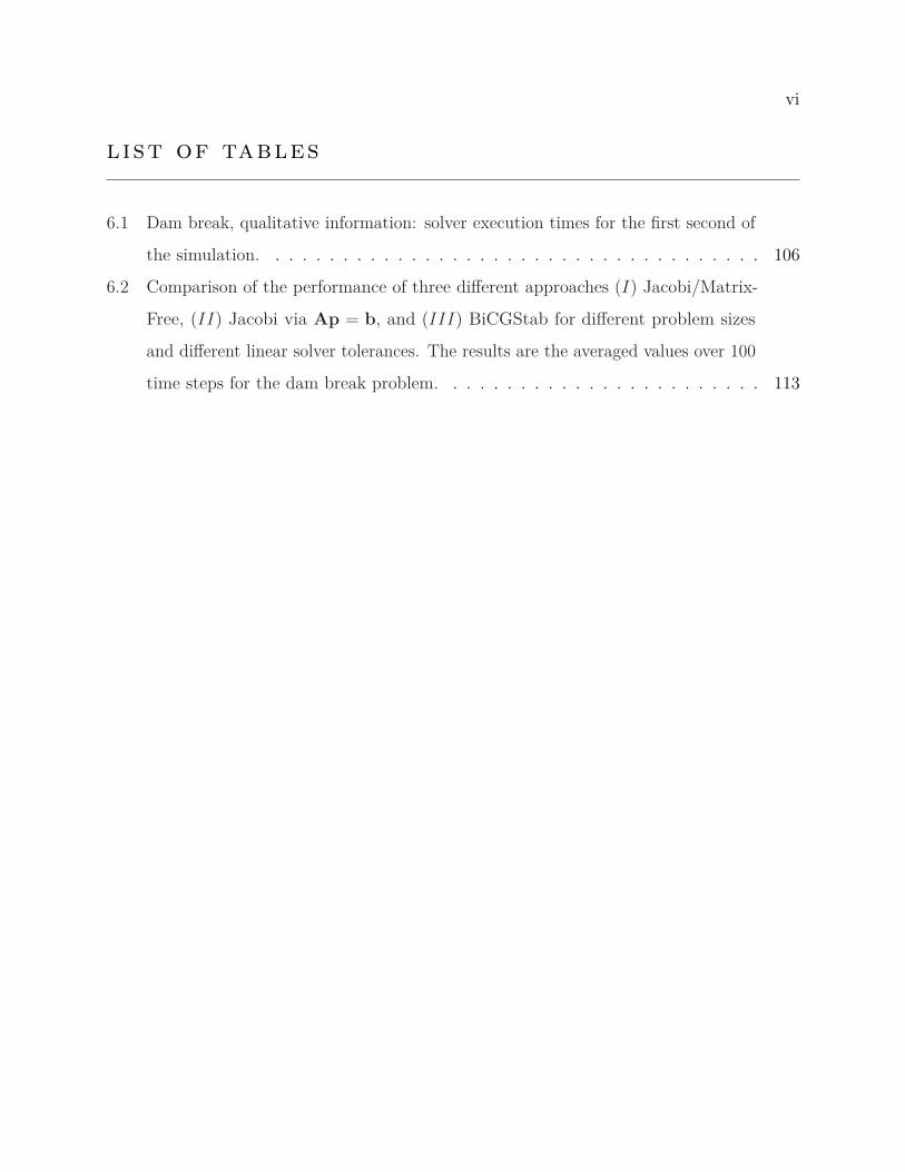
list of tables
6.1 Dam break, qualitative information: solver execution times for the first second of
the simulation. . . . . . . . . . . . . . . . . . . . . . . . . . . . . . . . . . . . . 106
6.2 Comparison of the performance of three different approaches (I) Jacobi/Matrix-
Free, (II) Jacobi via Ap = b, and (III) BiCGStab for different problem sizes
and different linear solver tolerances. The results are the averaged values over 100
time steps for the dam break problem. . . . . . . . . . . . . . . . . . . . . . . . 113

vii
list of figures
1.1 Schematic overview of the problems of interest in the present thesis. . . . . . . . 2
2.1 Illustration of the computational domains for non-conforming and conforming
mesh methods. . . . . . . . . . . . . . . . . . . . . . . . . . . . . . . . . . . . . 10
3.1 Schematic of contact between two bodies. . . . . . . . . . . . . . . . . . . . . . 16
3.2 ANCF cable element’s schematic. Each node features a global position vector and
a position vector gradient along the axis of the element (6DOF). Using shape
functions and knowing ξ one can interpolate the degrees of freedom to any point
P within the element. . . . . . . . . . . . . . . . . . . . . . . . . . . . . . . . . 24
3.3 ANCF shell element’s schematic. Global position vector rj and fiber’s direction
rjz = ∂rj
∂zi (ξi, ηj) are the nodal coordinates of the jth node (6DOF). Using shape
functions and knowing ξ and η one can interpolate the degrees of freedom to any
point within the element. . . . . . . . . . . . . . . . . . . . . . . . . . . . . . . 26
4.1 The control volume V bounded by the control surface S. At every point on the
control surface the vector n is pointing outward, and the f is the flux of a property
that enter or exit the control volume. . . . . . . . . . . . . . . . . . . . . . . . . 30
4.2 Stress/strain-rate relationship for different flow index and consistency parameters
in Herschel-Bulkley model [1]. . . . . . . . . . . . . . . . . . . . . . . . . . . . . 38
4.3 A mass-spring-damper system consisting of viscous, elastic, and frictional resistive
forces. . . . . . . . . . . . . . . . . . . . . . . . . . . . . . . . . . . . . . . . . . 41
4.4 2D illustration of the kernel W . The radius of the support domain is defined as a
multiple, κ, of the kernel’s characteristic length, h. . . . . . . . . . . . . . . . . 46
viii
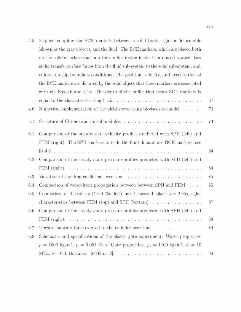
4.5 Explicit coupling via BCE markers between a solid body, rigid or deformable
(shown as the gray object), and the fluid. The BCE markers, which are placed both
on the solid’s surface and in a thin buffer region inside it, are used towards two
ends: transfer surface forces from the fluid sub-system to the solid sub-system; and,
enforce no-slip boundary conditions. The position, velocity, and acceleration of
the BCE markers are dictated by the solid object that these markers are associated
with via Eqs.3.6 and 3.18. The depth of the buffer that hosts BCE markers is
equal to the characteristic length κh. . . . . . . . . . . . . . . . . . . . . . . . . 67
4.6 Numerical implementation of the yield stress using bi-viscosity model. . . . . . . 71
5.1 Structure of Chrono and its submodules. . . . . . . . . . . . . . . . . . . . . . . 73
6.1 Comparison of the steady-state velocity profiles predicted with SPH (left) and
FEM (right). The SPH markers outside the fluid domain are BCE markers, see
§4.4.6. . . . . . . . . . . . . . . . . . . . . . . . . . . . . . . . . . . . . . . . . . 84
6.2 Comparison of the steady-state pressure profiles predicted with SPH (left) and
FEM (right). . . . . . . . . . . . . . . . . . . . . . . . . . . . . . . . . . . . . . 84
6.3 Variation of the drag coefficient over time. . . . . . . . . . . . . . . . . . . . . . 85
6.4 Comparison of water-front propagation between between SPH and FEM. . . . . 86
6.5 Comparison of the roll-up (t = 1.75s, left) and the second splash (t = 2.05s, right)
characteristics between FEM (top) and SPH (bottom) . . . . . . . . . . . . . . 87
6.6 Comparison of the steady-state pressure profiles predicted with SPH (left) and
FEM (right). . . . . . . . . . . . . . . . . . . . . . . . . . . . . . . . . . . . . . 89
6.7 Upward buoyant force exerted to the cylinder over time. . . . . . . . . . . . . . 89
6.8 Schematic and specifications of the elastic gate experiment. Water properties:
ρ = 1000 kg/m3, µ = 0.001 Pa·s. Gate properties: ρs = 1100 kg/m3, E = 10
MPa, ν = 0.4, thickness=0.005 m [2]. . . . . . . . . . . . . . . . . . . . . . . . 90
ix
6.9 Snapshots of the elastic gate simulation with FEM (top) and SPH(bottom). The
fluid domain is colored with the velocity magnitude. The x axis is horizontal,
pointing to the left; the y axis is vertical, pointing up. . . . . . . . . . . . . . . . 91
6.10 Comparison of the position of the tip of the gate between SPH, FEM and experi-
mental results [2]. . . . . . . . . . . . . . . . . . . . . . . . . . . . . . . . . . . . 92
6.11 Time variation of the average compressibility offset for the ISPH method. . . . . 94
6.12 Time variation of the average compressibility offset for the WCSPH method. . . 95
6.13 Time variation of the average compressibility offset for the KCSPH method. . . 96
6.14 Velocity profile of transient Poiseuille flow obtained from numerical simulation of
WCSPH, ISPH, and series solution at different times. . . . . . . . . . . . . . . . 97
6.15 Comparison of the steady-state velocity profiles predicted with WCSPH (left) and
ISPH (right). . . . . . . . . . . . . . . . . . . . . . . . . . . . . . . . . . . . . . 98
6.16 Comparison of the steady-state pressure profiles predicted with WCSPH (left)
and ISPH (right). . . . . . . . . . . . . . . . . . . . . . . . . . . . . . . . . . . . 99
6.17 Variation of the drag coefficient over time. . . . . . . . . . . . . . . . . . . . . . 100
6.18 Comparison of water-front propagation between between KCSPH (top), WCSPH
(middle), and ISPH (bottom). . . . . . . . . . . . . . . . . . . . . . . . . . . . . 101
6.19 Comparison of the roll-up (t = 1.75s, left) and the second splash (t = 2.05s, right)
characteristics between KCSPH (top), WCSPH (middle), and ISPH (bottom). . 101
6.20 Sloshing experiment: Comparison of fluid-structure interaction force along the
axis of periodic motion. . . . . . . . . . . . . . . . . . . . . . . . . . . . . . . . 103
6.21 IISPH vs. WCSPH (DualSPHysics [3]) comparison based on the relative drift in
the incompressibility. . . . . . . . . . . . . . . . . . . . . . . . . . . . . . . . . . 108
6.22 Comparison of the velocity profiles predicted with IISPH method (top) and
OpenFOAM (bottom). The SPH data was mapped to a grid for the sake of
comparison. . . . . . . . . . . . . . . . . . . . . . . . . . . . . . . . . . . . . . . 109
x
6.23 Comparison of the velocity profiles obtained with IISPH and OpenFOAM’s finite
volume method at two sections of the domain: center, x=0 m, and outlet, x=0.5 m.110
6.24 Schematic and specifications of the elastic gate experiment. Water properties:
ρ = 1000 kg/m3, µ = 0.001 Pa·s. Gate properties: ρs = 1100 kg/m3, E = 10
MPa, ν = 0.4, thickness=0.005 m [2]. . . . . . . . . . . . . . . . . . . . . . . . . 111
6.25 Comparison of the horizontal position of the tip of the elastic gate from the
numerical results of the present study, and the numerical/experimental results of
the study of Antoci et al. [2]. . . . . . . . . . . . . . . . . . . . . . . . . . . . . 111
6.26 Comparison of the convergence rate of the linear solver used in the current study
(GMRES and BiCGStab) vs. Jacobi method for a problem size of 55,000 for single
time step. . . . . . . . . . . . . . . . . . . . . . . . . . . . . . . . . . . . . . . . 112
6.27 Dam break example – scaling analysis of the pressure solver, the computational
bottleneck of the fluid-component solution. . . . . . . . . . . . . . . . . . . . . . 114
6.28 Configuration of the system in problem 1. β = 0.5 is chosen in §6.4.1 to ensure
all contacts are in the stick mode. . . . . . . . . . . . . . . . . . . . . . . . . . . 115
6.29 Normal (top) and tangential (bottom) contact forces without regularization (left),
and with a constant regularization (right). Contacts 1 and 2 are the leftmost,
contact 3 is the middle, and contacts 4 and 5 are the rightmost contacts in Fig. 6.28,
respectively. . . . . . . . . . . . . . . . . . . . . . . . . . . . . . . . . . . . . . 118
6.30 The tangential force is increased from 0 to 2.5N instead of a ramp function, while
other parameters remain similar to the ones in Fig. 6.29 . . . . . . . . . . . . . 119
6.31 Normal (top) and tangential (bottom) contact forces without regularization (left),
and with a constant regularization (right). Contacts 1 and 2 are the leftmost,
contact 3 is the middle, and contacts 4 and 5 are the rightmost contacts in Fig. 6.28,
respectively. . . . . . . . . . . . . . . . . . . . . . . . . . . . . . . . . . . . . . 120
6.32 The tangential force is increased from 0 to 2.5N instead of a ramp function, while
other parameters remain similar to the ones in Fig. 6.29 . . . . . . . . . . . . . 121

xi
6.33 A square box with the mass m = 1kg is placed on n2 spherical particles each with
diameter D. . . . . . . . . . . . . . . . . . . . . . . . . . . . . . . . . . . . . . 122
6.34 Variation of the mean and standard deviation of contact forces with number of
contacts predicted via the Gauss-Seidel method for the Tikhonov regularization
of α = 0.1. . . . . . . . . . . . . . . . . . . . . . . . . . . . . . . . . . . . . . . . 123
6.35 Variation of the mean and standard deviation of contact forces with number of
contacts predicted via the Gauss-Seidel method for the Tikhonov regularization
of α = 1.0. . . . . . . . . . . . . . . . . . . . . . . . . . . . . . . . . . . . . . . 123
6.36 Variation of the mean and standard deviation of contact forces with number of
contacts predicted via the APGD method for case (i). The APGD solver is robust
and predicts the analytical solution. . . . . . . . . . . . . . . . . . . . . . . . . . 124
6.37 Variation of the mean and standard deviation of contact forces with number of
contacts predicted via the APGD method for case (ii). The APGD solver is
unable to reach to an accurate solution while a small regularization parameter
can slightly improve the solution quality. . . . . . . . . . . . . . . . . . . . . . . 125
6.38 Variation of the mean and standard deviation of contact forces with number
of contacts predicted via the APGD method for case (iii). Similar to case (ii)
the APGD solver is unable to reach to an accurate solution but using larger
regularization parameter one can restore the solution quality. . . . . . . . . . . . 125
6.39 Configuration of the cannonball packing. Spheres have radius of 0.1m and mass
of 1kg. The initial spacing between the spheres is 2% of the radius. . . . . . . . 126
6.40 Frictionless cannonball packing configuration with N = 6. Each marker represents
a single contact, while solid-lines show ideal DEM-matched solutions. . . . . . . 127
6.41 Frictional cannonball packing configuration with N = 6. Each marker represents
a single contact, while solid-lines show ideal DEM-matched solutions. . . . . . . 128
6.42 Distribution of the normal force (z-direction) on the bottom particles in frictional
cannonball packing configuration with N = 6. . . . . . . . . . . . . . . . . . . . 129

xii
6.43 Distribution of the tangential force (x-direction) on the bottom particles in
frictional cannonball packing configuration with N = 6. . . . . . . . . . . . . . . 129
6.44 Distribution of the tangential (y-direction) force on the bottom particles in
frictional cannonball packing configuration with N = 6. . . . . . . . . . . . . . . 130
6.45 Frictional cannonball packing configuration with N = 11. Each marker represents
a single contact, while solid-lines show ideal DEM-matched solutions. . . . . . . 131
6.46 Distribution of the normal force (z-direction) on the bottom particles in frictional
cannonball packing configuration with N = 11. . . . . . . . . . . . . . . . . . . . 132
6.47 Distribution of the tangential force (x-direction) on the bottom particles in
frictional cannonball packing configuration with N = 11. . . . . . . . . . . . . . 133
6.48 Distribution of the tangential force (y-direction) on the bottom particles in
frictional cannonball packing configuration with N = 11. . . . . . . . . . . . . . 133
6.49 Frictional cannonball packing configuration with N = 21. Each marker represents
a single contact, while solid-lines show ideal DEM-matched solutions. . . . . . . 135
6.50 Distribution of the normal force (z-direction) on the bottom particles in frictional
cannonball packing configuration with N = 21. . . . . . . . . . . . . . . . . . . . 136
6.51 Distribution of the tangential force (x-direction) on the bottom particles in
frictional cannonball packing configuration with N = 21. . . . . . . . . . . . . . 137
6.52 Distribution of the tangential force (y-direction) on the bottom particles in
frictional cannonball packing configuration with N = 21. . . . . . . . . . . . . . 137
7.1 Triangular mesh for AC surface vs surface contact. The quad finite element mesh
is first converted to a triangular mesh composed of vertices, edges, and faces. Each
vertex is associated with a normal vector to compute interpenetrations. . . . . 142
xiii
7.2 Overview of the two-step simulation process. First, a musculoskeletal dynamic
simulation (COMAK), including an elastic foundation contact model, was used to
solve for tibiofemoral knee kinematics. Then, a novel deformable model was used
to estimate superficial cartilage strain at each instant in the gait cycle. Finally, the
average first principal strain directions were visually compared with experimental
split line maps ([4]) which represent collagen fiber alignment. . . . . . . . . . . . 142
7.3 Schematic comparison of the elastic foundation model (left) with the deformable
model (right) with the 2D section views on top. . . . . . . . . . . . . . . . . . . 143
7.4 Comparison of the net load results on the femur, medial and lateral cartilages
with theelastic foundation model [5]. . . . . . . . . . . . . . . . . . . . . . . . . 144
7.5 Comparison of articular cartilage inter-penetration (elastic foundation model) and
deflection (deformable model). Also see Fig. 7.3 . . . . . . . . . . . . . . . . . . 145
7.6 Different instants of time during the gait cycle when no internal pressure is applied.
First row: schematic of the motion during the gait cycle. Second row: deflection
field. Third row: maximum principal strains. Black lines show the first principal
strain directions and are scaled by the magnitude of the first principal strain at
each FE node. See Fig. 7.9 in supplementary information for corresponding tibial
plateau pressures and strain patterns. . . . . . . . . . . . . . . . . . . . . . . . . 147
7.7 Comparison of the fiber alignment predicted by this study for different scenarios
with experimental results [4] on the femur condyle. Histograms demonstrate the
distribution of the angle of deviation between the experimental split lines and
predicted principal strain directions. The dashed lines on histograms show the
median angle of deviation. See Fig. 7.9 in supplementary information for simulated
first principal strain directions on the tibial plateau. . . . . . . . . . . . . . . . . 148

xiv
7.8 Different instants of time during the gait cycle when no internal pressure is applied.
First row: schematic of the motion during the gait cycle. Second row: deflection
field. Third row: maximum principal strains (black lines show the maximum
principal strain directions and are scaled by the magnitude of the principal strain
at each FE node. . . . . . . . . . . . . . . . . . . . . . . . . . . . . . . . . . . . 149
7.9 Comparison of the average first principal strain directions induced via (a) tibiofemoral
loading during gait, (b) internal pressure and (c) coupled gait loading and internal
pressure. . . . . . . . . . . . . . . . . . . . . . . . . . . . . . . . . . . . . . . . . 150
7.10 The relative error of dimensionless normal force experienced by the side walls
of a bucket of material for different height (h) of material. The relative error is
calculated according to e = rf−rg
rf× 100, where rf is the non-dimensional averaged
fluid normal force and rg is the non-dimensional averaged granular normal force on
the side walls. The rg is calculated from the DEM simulation while rf is computed
from hydrostatic fluids. . . . . . . . . . . . . . . . . . . . . . . . . . . . . . . . . 154
7.11 Comparison of the front position in the dam break simulated with DEM and CFD.155
7.12 Comparison of the roll up (left) and the second splash (right) instances of the
dam break simulation between granular (bottom) and fluid (top) mediums. . . . 156
7.13 Comparison of the normalized horizontal force experienced by the cylinder in the
dam break simulation for different viscosities of the fluid and for different particle
diameters of the granular media. . . . . . . . . . . . . . . . . . . . . . . . . . . 157
7.14 Snapshots of the fluid (top) and the granular material (bottom) simulation of the
dam break with a cylindrical obstacle at t=1s (left), t=2s (middle), t=2.75s(right).158
7.15 Snapshots of the simulation of a fin slapping on the surface of water. (See [6]
Movie #137 for the animation) . . . . . . . . . . . . . . . . . . . . . . . . . . . 160
7.16 Snapshots of the interaction of a wedged shaped plate with water. . . . . . . . . 161
7.17 Fluid-solid interaction in the context of locomotion of bio-inspired under-water
robots. . . . . . . . . . . . . . . . . . . . . . . . . . . . . . . . . . . . . . . . . . 162

xv
8.1 Fluid-solid interaction modeling strategy of the articular cartilage . . . . . . . . 169
8.3 Preliminary results of the articular cartilage FSI model. Displacement and stress
field on the articular surface (top and bottom left, respectively). Pressure and
velocity distribution inside the interstitial fluid (top and bottom right, respectively)171

COMPUTATIONAL DYNAMICS OF CONTINUUM AND DISCRETE
SYSTEMS USING LAGRANGIAN METHODS
Milad Rakhsha
Under the supervision of Professor Dan Negrut
At the University of Wisconsin-Madison
This thesis investigates computational methods pertaining to multi-physics dynamics prob-
lems featuring continua, discrete systems, and their coupling. Specifically, computational
methods for solving governing equations of fluids, solids, and their interaction are studied in
a partitioned Lagrangian and parallel computing framework.
For fluid dynamics problems, the focus was on the use of Smoothed Particle Hydrodynamics
(SPH) as a Lagrangian discretization method for modeling and simulation of fluid flows. More
specifically, the Navier-Stokes equations are solved via an implicit-in-velocity and pressure
algorithm using a Chorin-style splitting technique for both Newtonian and non-Newtonian
fluid models. This implicit time integration allows for large time-steps while simulating a
broad spectrum of fluid flows ranging from highly viscous to flows with moderately large
Reynolds numbers in the laminar regime. The same continuum approach is adopted to resolve
the dynamics of discrete systems such as granular media by choosing a proper constitutive
equation for the deviatoric part of the stress tensor. The equivalence of the granular constitu-
tive equation to the Herschel-Bulkley fluid model allows for treating the granular material in
a continuum sense as a non-Newtonian fluid. A bi-viscosity model is employed to numerically
handle the yield stress within the Navier-Stokes framework.
For solid mechanics, the rigid-body dynamics governing equations account for frictional
contacts via a differential variational equality method along with an implicit time integration
scheme allowing for large time-steps. The uniqueness of the optimization problem arising
from frictional contacts is investigated and the Tikhonov regularization technique is used to
select the minimum norm solution. When bodies are flexible/compliant, their dynamics is

xvi
captured via the absolute nodal coordinate formulation, a non-linear finite element method
designed to handle simultaneously large deformations and large displacements/rotations.
Lastly, the two-way, dynamics coupling of the fluid and solid phases is done explicitly in a
partitioned framework. So-called Boundary Condition Enforcing (BCE) markers capturing
the motion of the solid phase are employed to impose no-slip and impenetrability conditions
for the fluid phase. Subsequently, the hydrodynamics forces are transferred to the rigid and
flexible multi-body dynamics systems as external forces.
The high computational load associated with the simulation of fluid-solid interaction problems
typically leads to long compute times. To address this issue, the software solution developed
under this work relies on: high-performance computing on graphics processing unit cards to
parallelize the fluid solver; and multi-core parallel computing and vectorization to accelerate
the rigid/flex-body dynamics solver. The software implementation of all algorithms discussed
in this work is publicly available on GitHub in an open-source C++ software package, called
Chrono, which is released under a permissive BSD3 license.
Dan Negrut

1
1 introduction
Computer simulation has opened up new research directions in many engineering and physical
sciences. The increased reliance of engineers and scientists on computer modeling and
simulation stems primarily from the relatively high cost of conducting experimental studies.
Harnessing the power of today’s computers to carry out billions of operations per second
can translate in some cases in replacing large amounts of experimental work with effective
computer simulation. In terms of continuum mechanics, current numerical methods can
simulate problems with millions of degrees of freedom. Similarly, simulating the dynamics
of many discrete systems with a relatively large number of degrees of freedom is possible.
However, computer simulation of (i) multidisciplinary problems featuring the coupling of
discrete systems and continua, and (ii) large scale discrete systems encountered in granular
media continue to pose many and interesting challenges.
1.1 Problem Statement
Problems involving the interaction of multiple physical phenomena are prevalent in many en-
gineering applications, ranging from biomechanics to geomechanics. Modeling and simulation
of soft tissues or cardiovascular flows are prime examples of multi-physics problems in biome-
chanics. Many environmental applications concerning renewable energy devices, offshore wind
turbines, etc., require modeling the dynamics of fluids, solids, and their interaction. Lastly,
a multi-physics modeling and simulation capability is required in geomechanics problems
encountered in partially saturated soil or landslides.
From the computational perspective, simulation of discrete systems poses a higher compu-
tational burden comparing to continuum modeling. For instance, discrete modeling of soil and
granular media leads to extremely large problems due to the small particle size and/or the
large number of particles in many real-world problems. A continuum approximation of these
systems could lead to more efficient solvers, yet the success of the homogenization process is
2
dictated by the predictive attribute of suitably chosen constitutive laws. The interest in this
Ph.D. thesis is in modeling the dynamics of both discrete and continuum systems as well as
their coupling, and, when possible, to use the continuum approach to approximate discrete
systems.
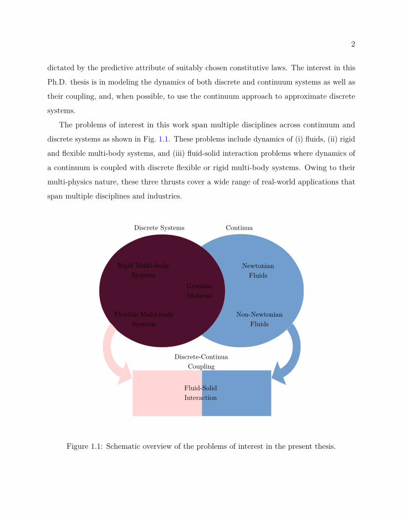
The problems of interest in this work span multiple disciplines across continuum and
discrete systems as shown in Fig. 1.1. These problems include dynamics of (i) fluids, (ii) rigid
and flexible multi-body systems, and (iii) fluid-solid interaction problems where dynamics of
a continuum is coupled with discrete flexible or rigid multi-body systems. Owing to their
multi-physics nature, these three thrusts cover a wide range of real-world applications that
span multiple disciplines and industries.
Newtonian Fluids
Non-Newtonian Fluids
GranularMaterial
Rigid Multi-body Systems
Flexible Multi-body Systems
Fluid-Solid Interaction
Discrete Systems Continua
Discrete-Continua Coupling
Figure 1.1: Schematic overview of the problems of interest in the present thesis.
3
1.2 Thesis Overview
This manuscript is organized as follows: Chapter 2 will provide a brief overview of the
existing work and literature on computational fluid dynamics, multi-body dynamics, and
fluid-solid interaction. Chapters 3 and 4 will discuss the modeling aspects and the numerical
methods for solving the governing equations of discrete and continuous systems, respectively.
Details about the software implementation of the framework are presented in Chapter 5, with
numerical experiments and validation discussed in Chapter 6. Chapter 7 presents several
applications and demonstrates the capabilities of the developed computational framework.
Conclusions and directions of future work are discussed in Chapter 8.
1.3 Summary of Contributions
The author’s work has led to the following archival publications: [7, 8, 9, 10, 11, 12, 13]. The
specific contributions of the author are summarized as follows:
• Investigated the use of SPH for the Navier-Stokes equations
– Investigated four different SPH methods (WCSPH, ISPH, KCSPH, and IISPH)
and their solution attributes
– Performed a comparison between Implicit SPH (ISPH), Weakly Compressible SPH
(WCSPH), and Kinematically Constrained SPH (KCSPH)
– Compared and contrasted the solution attributes of SPH as a Lagrangian method
against continuous finite element method for free-surface and fluid-solid interaction
problems
– Implemented and improved the Implicit Incompressible SPH [14] method by solving
the discretized Poisson pressure equation via advanced linear solvers
– Implemented and validated a projection-based implicit, both velocity and pressure,
solver that can handle a wide range of fluid flows ranging from highly viscous flows
to flows with moderately large Reynolds numbers in the laminar regime

4
– Investigated the use of consistent SPH discretization for internal flow problems
– Implemented the Herschel-Bulkley fluid model for modeling and simulation of
non-Newtonian fluids
– Investigated the use of ISPH method for modeling and simulation of granular
dynamics as a non-Newtonian fluid
• Investigated the solution quality in frictional-contact problems and demonstrated insights
gained in the context of a biomechanics application
– Investigated the use of the Tikhonov regularization method for imparting unique-
ness to the distribution of frictional contact forces in granular dynamics problems
solved via a differential variational inequality approach
– Simulated the tibiofemoral cartilage contact during walking for the prediction of
collagen fiber orientation
• Developed a partitioned fluid-solid interaction framework
– Coupled the fluid solver to a multi-body engine capable of simulating rigid and
flexible bodies interacting through frictional contact
– Validated the fluid-structure coupling via benchmark experiments featuring flexible
and rigid elements
• Leveraged hybrid CPU/GPU parallelization to improve the performance of the FSI
framework
– Implemented SPH on GPU cards using CUDA to leverage high memory bandwidth
– Implemented Krylov linear solvers such as GMRES and BiCGStab on GPU to
improve the efficiency of the underlying linear solvers
– Leveraged OpenMP for parallelism of the flexible multi-body dynamics solver on
the CPU
– Improved the efficiency of the low-level matrix operation on the host code via AVX
vectorization intrinsics
5
2 background
This chapter will provide brief background information about different types of physics studied
in this manuscript. These include the dynamics of fluids, rigid and flexible multibody systems.
Lastly, methods concerning the coupling between fluids and solids are discussed as well.
2.1 Computational Fluid Dynamics
Computational fluid dynamics is a significant branch of computational continuum mechanics,
and it is concerned with the simulation of continua using computers. Many aspects of CFD
have been studied in the past. This includes various space discretization and time integration
schemes. Insofar as the space discretization step is concerned, the majority of CFD models
can be classified as: (i) Eulerian approaches, where the unknown state variables are attached
to stationary observers; or (ii) Lagrangian approaches, in which the unknown state variables
are attached to moving observers.
Eulerian methods have been successfully applied and are very popular in CFD. Indeed,
Finite Difference (FD) represents a robust technique for solving partial differential equations
on simple domains, while the Finite Volume (FV) has been predominantly applied in fluid
flows with complex geometries. Conversely, the Lagrangian methods gained traction only
about two decades ago, although the idea of using Lagrangian discretization dates back to
1957 [15]. Among Lagrangian methods, SPH [16, 17] has been widely adopted as the low-order
approximation of choice for a variety of problems [18], while Moving Least Squares and Radial
Basis Functions emerged as the leading high-order meshless methods [19, 20, 21, 22].
For FSI problems, just as for free-surface flows, the Eulerian approaches are challenged by
large mesh deformations, which call upon re-meshing operations. A widely used approach is
the Arbitrary Lagrangian-Eulerian (ALE) method [23], which handles well sufficiently small
mesh deformation, yet it becomes expensive when the motion of the solid objects is relatively
large. The Immersed Boundary Method (IBM) [24] addresses this shortcoming by implicitly

6
treating the solid objects, as opposed to the ALE explicit representation of solid bodies that
calls for body-fitted meshing. Thus, IBM alleviates the mesh deformation problem at the
cost of a higher mesh resolution in the vicinity of the solid objects.
Handling FSI problems comes more naturally to meshless methods, e.g. SPH, owing to
their Lagrangian nature that interfaces well with the Lagrangian framework used in solid
mechanics. However, SPH-based methods generally have enjoyed a somewhat limited adoption
due to their reduced order and deficiencies in numerical approximation near boundaries [19].
Kernel-correction methods have been recently proposed to enforce linear consistency and
second-order accuracy, yet they alter the conservation properties of SPH [25, 26, 27, 28, 29].
Likewise, the use of larger support basis functions improves robustness but leads to a higher
computational cost.
Amongst different choices of discretization methods, in this thesis, SPH is embraced for
space discretization of the underlying equations owing to its strength in solving free-surface,
large-deformation, and fluid-solid interaction problems. SPH comes in many different formu-
lations as far as time-integration, compressibility level, and boundary condition treatment
are concerned, which will be further discussed in later chapters.
2.2 Computational Multibody Dynamics
A multibody system is defined as a collection of bodies interacting through mechanical
constraints and frictional contact between the objects. Joints constrain the relative motion
of bodies while springs and dampers induce additional loads in the system. Each body
posses a specific mass and shape while the interconnects are treated as massless. These
modeling assumptions apply to a large class of mechanical systems, from robots and vehicles
to biomechanical systems [30]. Computational multibody dynamics is the term used herein
to refer to the numerical modeling technique used for resolving the dynamics of these discrete
systems. Depending on the stiffness of discrete objects being studied, multibody systems may
be further categorized into rigid multibody systems and flexible multibody systems.

7
2.2.1 Rigid Multibody Systems
A large body of literature is dedicated to rigid multibody systems featuring mechanical
joints/constraints [31, 32]. When frictional-contact between objects is present, existing
methods may be categorized in two groups: penalty and complementarity methods.
In penalty methods, the fundamental assumption is that bodies, although being rigid,
deform slightly at the point of contact. The inter-penetration between the rigid bodies
calculated during the proximity-computation stage is used to penalize further inter-penetration
by creating contact forces between bodies through fictitious springs and dampers [33, 34, 35].
The process of choosing the model parameters and the simplification of the contact geometry
are two main drawbacks of this method. Despite its shortcomings, penalty method has
been used in numerous numerical studies on the dynamics of large rigid body systems
[36, 37, 38, 39, 40, 41].
In the complementarity (constraint-based) approach, the main idea is to modify the
equations of motion to include a differential inclusion [42] and to impose non-penetration
between rigid bodies through constraints enforced by applying impulses. This method has
been modified to model rolling and spinning friction in addition to sliding friction [43]. An
important drawback associated with this method is the lack of uniqueness in the set of contact
forces resulting from the solution of an optimization problem. In the present work, the
complementarity method is employed to resolve the dynamics of contact between rigid bodies,
while the penalty approach is used to handle contact between deformable bodies.
2.2.2 Flexible Multibody Systems
Unlike the rigid body dynamics where there is no distinction between the kinematics of the
body and its reference frame, further modeling is required to capture the deformation of
elastic components in flexible body dynamics. This is mainly because the distance between
two points on/inside a deformable body changes, and the kinematics of the reference frame
cannot sufficiently describe the time evolution of the flexible component. To this end, elastic

8
components are discretized in space to study their motion via a finite number of degrees of
freedom. This is in contrast to rigid multibody systems where each rigid object is uniquely
defined, regardless of its shape, by a set of position and orientation degrees of freedom. The
final stage of the solution consists of solving for state variables, including those associated
with rigid body motion as well as those defining elastic displacements and/or position and
orientation of the discretized nodes. The Floating Frame of Reference (FFR), co-rotational
formulation, and Absolute Nodal Coordinate Formulation (ANCF) are three of the most
relevant formulations in the context of flexible multibody systems.
In the FFR formulation, the position of a point in the flexible body is expressed as the
superposition of a small (flexible) deformation, described in the body coordinate system, and
possibly large translation and rotation of the body’s coordinate system. The deformation
of the body with respect to its coordinate system is expressed via the nodal coordinates of
the discretized finite elements. The finite element used in the FFR formulation leads to zero
strain under any arbitrary rigid body motion of the flexible object. Despite being the most
widely used formulation in the computational flexible body dynamics, FFR is limited to cases
where the deformation of the flexible body with respect to its reference frame is small. See
[44, 45] for more details about the FFR formulation.
The ANCF is a non-linear finite element method formulated to handle large deformations.
In ANCF, no co-rotated frame is used to describe the kinematics of deformed finite elements.
Most importantly, the distinguishing feature of ANCF is the use of position vector gradients
to describe the rotation of the body as well as its strain state, thereby avoiding the need
for interpolating non-vectorial rotation parameters. Given the interest of the present work
in problems featuring large deformations and driven by the limitations of the FFR for such
problems, the ANCF method is chosen in the present work.

9
2.3 Fluid-Solid Interaction
Many engineering applications, e.g., cardiovascular flows, fluid sloshing, particles in suspension,
etc., require the solution of an FSI problem. Some of these problems involve large deformations,
in which case the fluid-solid coupling remains challenging to solve [46]. For most FSI problems,
it is nearly impossible to obtain analytical solutions. Additionally, laboratory experiments
are also limited and costly to conduct [47]. Thus, numerical simulations must be employed.
Different classifications exist in the context of numerical methods for FSI problems.
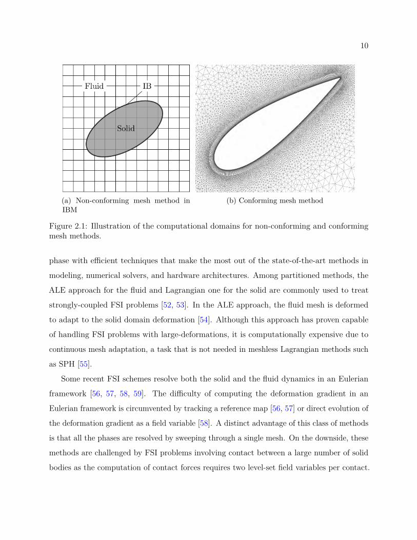
One classification is to consider the computational domain and divide the methods into
conforming mesh methods and non-conforming mesh methods. In the conforming mesh
methodology, the computational domains of sub-systems match at the interface, while in
non-conforming mesh methods the computational domain of the fluid sub-system serves more
as a background mesh for the solid phase. As an example of non-conforming mesh methods, in
IBM [48, 49], the immersed boundary is tracked in a Lagrangian fashion; the fluid is tracked
in an Eulerian framework on a non-conforming and regular grid; lastly, the presence of the
immersed boundary on the non-conforming grid is included in Navier-Stokes equations as
extra source terms. Fig. 2.1 illustrates the difference between the computational domains of
the aforementioned methods. The approach to be taken in the current work does not fit into
this classification since a mesh-less method is to be used for the fluid phase. However, the
methodology is more similar to conforming mesh methods.
Another classification pertains to the sequence of the solution algorithms and the governing
equation of the overall system. Accordingly, FSI methods are grouped into monolithic and
partitioned approaches. In the former [50, 46, 51], the governing equations of the fluid and
the solid phases are solved simultaneously; the interfacial conditions are implicit in the
solution procedure; and potentially a better accuracy can be obtained for a multidisciplinary
problem [47]. In contrast, in the latter approach, the two phases are solved separately, and
the solutions are usually explicitly coupled together. Each method has its advantages and
drawbacks. What makes the partitioned approach appealing is the fact that it solves each
10
(a) Non-conforming mesh method inIBM
(b) Conforming mesh method
Figure 2.1: Illustration of the computational domains for non-conforming and conformingmesh methods.
phase with efficient techniques that make the most out of the state-of-the-art methods in
modeling, numerical solvers, and hardware architectures. Among partitioned methods, the
ALE approach for the fluid and Lagrangian one for the solid are commonly used to treat
strongly-coupled FSI problems [52, 53]. In the ALE approach, the fluid mesh is deformed
to adapt to the solid domain deformation [54]. Although this approach has proven capable
of handling FSI problems with large-deformations, it is computationally expensive due to
continuous mesh adaptation, a task that is not needed in meshless Lagrangian methods such
as SPH [55].
Some recent FSI schemes resolve both the solid and the fluid dynamics in an Eulerian
framework [56, 57, 58, 59]. The difficulty of computing the deformation gradient in an
Eulerian framework is circumvented by tracking a reference map [56, 57] or direct evolution of
the deformation gradient as a field variable [58]. A distinct advantage of this class of methods
is that all the phases are resolved by sweeping through a single mesh. On the downside, these
methods are challenged by FSI problems involving contact between a large number of solid
bodies as the computation of contact forces requires two level-set field variables per contact.

11
Storing these field variables becomes expensive in comparison to O(1) state variables that
are stored in Lagrangian formulations [56] for each contact.
In the present research, the Fluid-Solid Interaction method will be resolved in a Lagrangian-
Lagrangian framework. Similar fluid-structure coupling was discussed in [60] and further
improved in [54, 61, 62]. In [60], the contact forces were calculated based on an iterative
master-slave scheme, which finds the best penalty forces required for the no-penetration
condition. A similar but non-iterative scheme was used in [62]. In [54, 63], a dummy-particles
scheme was used to compute the pressure from the fluid side. The present work follows in
the footsteps of this last approach.
2.4 Granular Flows
While water is the most handled industrial material, granular material is the second. Dense
granular flows, however, are substantially more complex than their fluid counterparts. Granular
material is essentially a discrete system whose evolution is described by the Newton-Euler’s
equations featuring frictional contact force (see Eq. 3.4). Although the discrete representation
can accurately capture the motion of granular flows, the fully resolved modeling of large scale
granular flows is a challenging task owing to (i) their complex frictional contact interactions,
and (ii) a high computational burden as the motion of individual particles needs to be tracked
in a numerical integration framework that advances simulation at time steps ∆t ≈ 10−5 or
lower. To address the latter aspect, discrete granular flow simulations use parallel computing
to accelerate the computations. To date, the largest granular dynamics simulation of practical
relevance contained 2.4 billion bodies, which was run on 16,384 CPUs (131,072 cores) of
Japan’s K-computer [64, 65], the 2012 fastest supercomputer in the world and now the 18th
in the ranking of the world’s supercomputers [66].
The collective behavior of individual particles may, however, be regarded as a continuum.
Given that granular media can demonstrate distinctively different behaviors under various
local stress conditions, the focus of this research is on the fluid-like evolution of granular
12
material that happens when it is rapidly sheared. In such cases, (i) shear stress in granular
material shows strain-rate dependency, which is a characteristic of fluids and, (ii) there exists
a threshold value (yield criterion), under which the grains do not flow, a characteristic of
solid materials. These features suggest a viscoplastic behavior of a granular material which is
similar in nature to that of non-Newtonian fluids such as Bingham liquids [67, 68].
Constitutive laws that could describe the motion of granular flows are still lacking.
Amongst various models and theories developed previously, the µ(I)-rheology [67] is one
of the successful frameworks describing observations from a variety of experimental and
numerical results.
In the present work, we describe the fully resolved modeling of granular flows via the
complementarity approach described in §2.2.1.
13
3 discrete systems
Contrary to continua, in discrete systems the motion of individual objects in the system
and their interactions on each other is studied. In the following section, the mathematical
formulations of such systems are described.
Definitions
Throughout section §3, the following conventions are used to denote the quantities associated
with discrete systems. Scalar variables are denoted by uppercase or lowercase lightface Latin
and Greek letters, e.g. ρ and φ. Vectors are denoted via bold, lowercase Latin letters, e.g. x
and they are column vectors unless otherwise specified. More specifically, the variables x, v,
a are used to represent the position, velocity and acceleration of an object. Indexed vectors
are used to specify either an element of the vector or an object in the vector depending on the
context, e.g. xi is the position of body i. The first time-derivative is represented with over
dot, e.g. x = v. The second time-derivative is denoted via over double-dot, e.g. x = v = a.
Matrices are represented as bold uppercase Latin letters, e.g. M . One subscript is used to
specify a single row, e.g. Mi for row i in the matrix M . Two subscripts are used to indicate a
specific row and column, e.g. Mi,j . The Frobenius norm of a matrix or a vector is defined as
‖ ∗ ‖F . The skew-symmetric cross product operator for a three dimensional vector is defined
as follows and results in a 3× 3 matrix
s =
0 −sz sy
sz 0 −sx−sy sx 0.
(3.1)

14
3.1 Rigid Body Dynamics
In this section we describe the dynamic systems featuring rigid bodies and frictional contact
between them. As explained in Section §2.2.1, a complementarity-based approach is used to
resolve the contact between different objects.
Preamble
“Rigid body” refers to a 3D object that can translate and rotate in space. The set of generalized
coordinates that describe the position and orientation of a body in the 3D Euclidean space
are rj ∈ R3 and εj ∈ R4, which are respectively the absolute position of the center of mass,
and Euler parameters associated with orientation of body j. Combining the set of generalized
coordinates of different bodies for a system of nb bodies, one can write the set of generalized
coordinates describing the system at position level as x =[rT1 , ε
T1 , . . . , r
Tnb, εTnb
]T∈ R7nb , and
at velocity level as x =[rT1 , ε
T1 , . . . , r
Tnb, εTnb
]T∈ R7nb . One can choose to use angular velocities
instead of the time derivative of the Euler parameters to describe the system at the velocity level
by v =[rT1 , ω
T1 , . . . , r
Tnb, ωTnb
]T∈ R6nb , which reduces the problem size. The transformation
from the derivatives of Euler parameters, εB, to angular velocities at the body-fixed frame, ωB,
for each body is governed by εB = 12G
T (εB)ωB, where matrix G ∈ R3×4 depends linearly on
the Euler parameters εB. Therefore, if one chooses to work with Euler angles at the velocity
level, the block diagonal matrix L(q) ≡ diag[I3×3,
12G
T (ε1), . . . , I3×3,12G
T (εnb)]∈ R7nb×6nb
can be used to obtain x = L(q)v, the time derivative of the set of generalized coordinate
describing the system, where I3×3 is the identity matrix [31].
3.1.1 Bilateral Constraints
A bilateral constraint represents a kinematic relationship between generalized coordinates
in a discrete system. Spherical joints, prismatic joints, or revolute joints are examples of
mechanical constraints that are comprised of a set of bilateral constraints represented by

15
B. Hence, gi (q, t) = 0, i ∈ B is a set of scalar equations to enforce kinematic constraints
through algebraic equality equations. For instance, a revolute joint imposes five constraint
equations, while a spherical is comprised of three constraint equations [31].
The velocity-level constraint equations which must be satisfied are obtained by taking
time-derivative of the constraints as ∇qgTi L (q)v + ∂gi
∂t= 0.
3.1.2 Unilateral Constraints and Frictional Contact
In the Differential Variational Inequality (DVI) [69] approach the equations of motion are
modified to include a differential inclusion [42] and to impose non-penetration between rigid
bodies through constraints enforced by applying impulses. After discretization this problem
is posed as an optimization problem with complementarity and equilibrium constraints.
More specifically, the three-dimensional Coulomb friction assumption leads to a Non-linear
Complementarity Problem (NCP). In what follows, more details about the theory of the
complementarity approach are explained.
Consider a contact between bodies A and B as shown in Fig. 3.1. The tangent plane at
the contact point for the contact i is defined by vectors ui, wi and the normal ni in Fig. 3.1.
A local reference frame can be defined for each body at the contact point based on these
vectors. For body A, the normal to the tangent plane, ni,A, points toward body B. The two
mutually orthogonal vectors ui,A, and wi,A are defined using the Gram-Schmidt method. The
same methodology is used to build the local reference frame at the contact point i, for body
B with wi,B, ui,B, and ni,B ∈ R3.
If the gap (distance) between bodies A and B at the contact point is defined by Φ, a
complementarity condition can be defined as 0 ≤ γci,n ⊥ Φ ≥ 0, where γci,n is the Lagrange
multiplier associated with the contact i. The complementarity condition states that at least
one of the γci,n, or Φ is zero; when the gap function is zero, the normal contact force is greater
than zero and when the normal contact force is zero the gap function is greater than zero
(there is no contact between body A and B). The contact force associated with contact

16
Figure 3.1: Schematic of contact between two bodies.
i can be expressed as fi,N = γci,nni, and fi,T = γci,uui + γci,wwi which are the normal and
tangential forces, respectively. γci,w, γci,u, and γci,n are the magnitude of the contact forces in
each direction. The Coulomb dry-friction model based on the friction forces is expressed as
[70, 71]
√(γci,u)2 + (γci,w)2 ≤ µfi γ
ci,n, (3.2a)
‖vi,T‖(√
(γci,u)2 + (γci,w)2 − µfi γci,n)
= 0, (3.2b)
〈fi,T ,vi,T 〉 = −‖fi,T‖‖vi,T‖ , (3.2c)
where vi,T denotes the relative tangential velocity between bodies A and B at the contact
point. More specifically, Eq. 3.2a states that the the friction force is less than the normal force
times the friction coefficient. Eq. 3.2b states a complementarity condition where equality
condition of Eq. 3.2a holds if the vi,T 6= 0, and inequality of Eq. 3.2a holds if vi,T = 0. Lastly,
Eq. 3.2c states that the friction force is in the opposite direction of vi,T . If now one considers

17
the following constraint minimization problem,
(γci,u, γ
ci,w
)= argmin√
(γci,u)2+(γc
i,w)2≤µfi γ
ci,n
vTi,T(γci,uui + γci,wwi
), (3.3)
then Eq. 3.2a-3.2c represent the first order Karush-Kuhn-Tucker optimality condition for
the above optimization problem with respect to γci,u, and γci,w variables. Hence, the Coulomb
friction model is implemented as a constraint optimization problem. Finally, the contact
force at the ith contact point is expressed as fi = fi,N + fi,T = γci,nni + γci,wui + γci,wwi ∈ Υi,
where Υi is a 3D cone of slope tan−1(µfi ) and oriented along ni, i.e., Υi = [x, y, z]T ∈
R3|√y2 + z2 ≤ µfi x.
The Newton-Euler equations of motion for the system [70] are expressed as:
q = L(q)v,
Mv = f (t,q,v)− gTq (q, t)λ+ ∑i∈A(q,δ)
(γi,n Di,n + γi,u Di,u + γi,w Di,w) ,
0 = g(q, t),
i ∈ A(q(t), δ) : 0 ≤ γi,n ⊥ Φi(q) ≥ 0,
(γi,u, γi,w) = argmin√(γc
i,u)2+(γci,w)2≤µf
i γci,n
vT(γci,u Di,u + γci,w Di,w
),
(3.4)
where f(t,q,v) are the external forces, M is the system mass Matrix, A(q, δ) is the set of
active and potential unilateral constraints based on the bodies that are mutually less than
δ apart, and g(q, t) is the set of bilateral constraints acting on the system and gTq (q, t) is
the Jacobian of the constraints with respect to the generalized coordinates. Moreover, the
tangent space generators Di = [ Di,n, Di,u, Di,w] ∈ R6nb×3 are defined as
DTi =
[0 . . . −AT
i,p ATi,pAA
˜si,A 0 . . . 0 ATi,p −AT
i,pAB˜si,B . . . 0
], (3.5)
18
where Ai,p = [ni,ui,wi] ∈ R3×3 is the orientation matrix associated with contact i, AA =
A (εA) and AB = A (εB) are the rotation matrices of bodies A and B respectively; the vectors
si,A and si,B ∈ R3 represent the contact point positions in body-relative coordinates as shown
in Fig. 3.1. More details about the solution algorithm, and time-stepping scheme of the this
DVI problem may be found in [70, 72, 73].
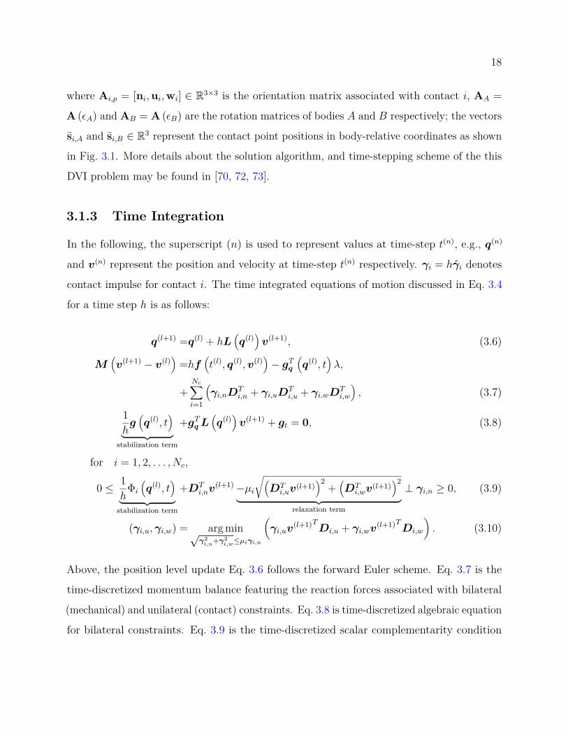
3.1.3 Time Integration
In the following, the superscript (n) is used to represent values at time-step t(n), e.g., q(n)
and v(n) represent the position and velocity at time-step t(n) respectively. γi = hγi denotes
contact impulse for contact i. The time integrated equations of motion discussed in Eq. 3.4
for a time step h is as follows:
q(l+1) =q(l) + hL(q(l)
)v(l+1), (3.6)
M(v(l+1) − v(l)
)=hf
(t(l), q(l),v(l)
)− gTq
(q(l), t
)λ,
+Nc∑i=1
(γi,nD
Ti,n + γi,uDT
i,u + γi,wDTi,w
), (3.7)
1hg(q(l), t
)︸ ︷︷ ︸
stabilization term
+gTqL(q(l)
)v(l+1) + gt = 0, (3.8)
for i = 1, 2, . . . , Nc,
0 ≤ 1h
Φi
(q(l), t
)︸ ︷︷ ︸stabilization term
+DTi,nv
(l+1)−µi√(DT
i,uv(l+1)
)2+(DT
i,wv(l+1)
)2
︸ ︷︷ ︸relaxation term
⊥ γi,n ≥ 0, (3.9)
(γi,u,γi,w) = arg min√γ2
i,u+γ2i,w≤µiγi,n
(γi,uv
(l+1)TDi,u + γi,wv(l+1)TDi,w
). (3.10)
Above, the position level update Eq. 3.6 follows the forward Euler scheme. Eq. 3.7 is the
time-discretized momentum balance featuring the reaction forces associated with bilateral
(mechanical) and unilateral (contact) constraints. Eq. 3.8 is time-discretized algebraic equation
for bilateral constraints. Eq. 3.9 is the time-discretized scalar complementarity condition
19
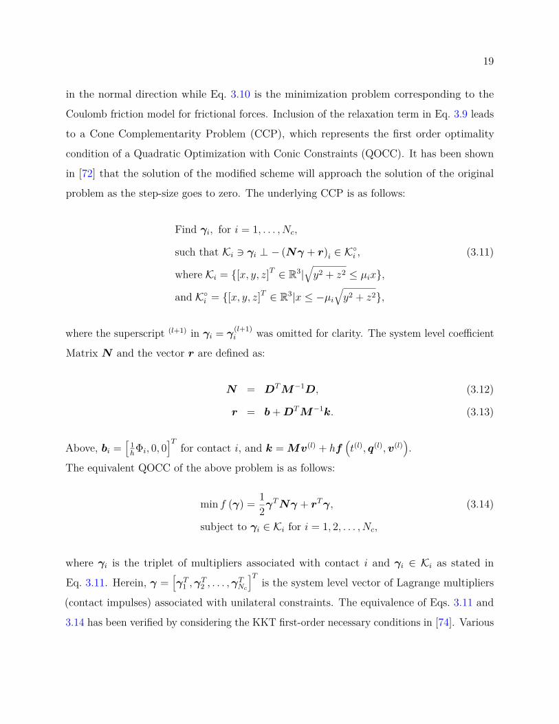
in the normal direction while Eq. 3.10 is the minimization problem corresponding to the
Coulomb friction model for frictional forces. Inclusion of the relaxation term in Eq. 3.9 leads
to a Cone Complementarity Problem (CCP), which represents the first order optimality
condition of a Quadratic Optimization with Conic Constraints (QOCC). It has been shown
in [72] that the solution of the modified scheme will approach the solution of the original
problem as the step-size goes to zero. The underlying CCP is as follows:
Find γi, for i = 1, . . . , Nc,
such that Ki 3 γi ⊥ − (Nγ + r)i ∈ Ki , (3.11)
where Ki = [x, y, z]T ∈ R3|√y2 + z2 ≤ µix,
and Ki = [x, y, z]T ∈ R3|x ≤ −µi√y2 + z2,
where the superscript (l+1) in γi = γ(l+1)i was omitted for clarity. The system level coefficient
Matrix N and the vector r are defined as:
N = DTM−1D, (3.12)
r = b+DTM−1k. (3.13)
Above, bi =[
1hΦi, 0, 0
]Tfor contact i, and k = Mv(l) + hf
(t(l), q(l),v(l)
).
The equivalent QOCC of the above problem is as follows:
min f (γ) = 12γ
TNγ + rTγ, (3.14)
subject to γi ∈ Ki for i = 1, 2, . . . , Nc,
where γi is the triplet of multipliers associated with contact i and γi ∈ Ki as stated in
Eq. 3.11. Herein, γ =[γT1 ,γ
T2 , . . . ,γ
TNc
]Tis the system level vector of Lagrange multipliers
(contact impulses) associated with unilateral constraints. The equivalence of Eqs. 3.11 and
3.14 has been verified by considering the KKT first-order necessary conditions in [74]. Various

20
methods exist for solving Eqs. 3.11 and 3.14. In [74] advantages and shortcomings of solution
algorithms such as Jacobi, Gauss-Siedel, Accelerated Projected Gradient Descent (APGD),
and interior-point method for solution of the problem in its optimization form, Eq.3.14, were
discussed.
3.1.4 Solution Uniqueness
The complementarity method discussed in Eqs. 3.11 or 3.14 for idealized perfectly-rigid bodies
does not have a unique solution. Specifically, this is due to the indeterminacy of the curvature
matrix N , which is typically positive semidefinite. A positive semidefinite matrix N emerges
when there are many contacts per body. Thus, the system has infinitely many sets of reaction
forces that satisfy the DVI equations. This non-uniqueness appears only in the normal forces
for frictionless problems, while both the velocities and the contact forces are non-unique for
frictional problems. Use of additional compatibility conditions for contact forces in frictionless
problems was investigated in [75]. The compatibility condition maintains no-penetration
constraints but filters out force distributions that could not have arisen from stiff elastic
contacts. In the present work, we use the Tikhonov regularization method to improve the
solution quality in frictional problems. Herein, the set of solution to Eq. 3.14 is denoted by
S = γ ∈ K | f(γ) = infy∈K
f(y), (3.15)
where K = K1 ×K2 . . .×KNc is the direct product of the individual contact cones.
The Tikhonov regularized QOCC of Eq. 3.14 is modified as:
min fα (γ) = 12γ
TNγ + rTγ + α‖γ‖2W , (3.16)
subject to γi ∈ Ki for i = 1, 2, . . . , Nc.
The inclusion of the regularization term α‖γ‖2W increases the zero eigenvalues of the N to
ensure a unique solution. Note that the cost function in Eq. 3.16 is strictly convex for α > 0.

21
According to the Tikhonov regularization method, the minimum-norm solution of a
convex optimization problem may be obtained by solving a sequence of related strongly convex
optimization problems. Accordingly, the sequence γk generated by the Tikhonov regularized
problem
γk+1 = argminγ∈K
12γ
TNγ + rTγ + αk‖γ‖2W, (3.17)
converges to the minimum norm of S as α → 0+, which is sufficient from the theoretical
perspective. However, one may choose not to find the exact solution of each subproblem, but
solving it withing some tolerance εk, in order to make the solution procedure more efficient.
The idea is to solve the subproblem with looser tolerances at the beginning and with more
strict tolerances as α → 0+. In practice, one may choose to reduce the tolerance and the
regularization parameter as εk+1 = τεεk and αk+1 = τααk, for some constants τα and τε, where
0 < τε < τα < 1.
Alternatively, one may choose a small value of the regularization parameter αk and solve
only one subproblem and since the feasible set is convex for α > 0. This regularized problem
has a unique solution although the solution may slightly differ from the classical Tikhonov
regularization method described above. These ideas are investigated for a few benchmark
problems in section §6.4.
3.2 Flexible Body Dynamics
The nonlinear flexible body dynamics formulation used in the current work draws on ANCF, a
nonlinear finite element formulation introduced by Shabana [44] to describe large deformation
of moving bodies. The salient feature of ANCF is the use of position vector gradients to
describe the rotation of the body. ANCF uses the nodal global-position and the nodal position-
vector-gradients to describe the nonlinear dynamics of flexible bodies that can undergo large
22
deformation. In general, the position field of ith ANCF element may be defined as:
ri(ξ, η, ζ, t)︸ ︷︷ ︸Position of an arbitrarypoint within the element
= S(ξ, η, ζ)︸ ︷︷ ︸Space-dependentshape function
× qi(t),︸ ︷︷ ︸Time-dependent vector ofnodal degrees of freedom
(3.18)
which simply gives the position of any point (ξ, η, ζ) ∈ [−1, 1] inside the element at time
t based on interpolation (S(ξ, η, ζ)) of the nodal coordinates (qi(t)). Due to the fact that
description of elements is in global coordinates, the inertia forces have a simple form in ANCF
elements. The velocity of any point within an element i may be written as
ri(ξ, η, ζ, t)︸ ︷︷ ︸Velocity of an arbitrarypoint within the element
= S(ξ, η, ζ)︸ ︷︷ ︸Space-dependentshape function
× qi(t).︸ ︷︷ ︸Time-dependent vector of
generalized velocities
(3.19)
The kinetic energy of a finite element i can be obtained as
T = 12
∫V
ρriTri dV = 12 qiTMqi , (3.20)
where the mass matrix M is defined as M =∫A ρAS
TS dx, which is time-independent. The
equations of motion assume the form [32]
Mq + Qe = Qa , (3.21)
where Qe and Qa are the generalized element elastic and applied forces, respectively. The description
of these elements and calculation of the internal forces are described in §3.2.1, and §3.2.2.
ANCF elements may be classified based on the number of position vector gradients defined at
each node. (i) Fully parameterized ANCF elements use position vector r ∈ R3, and 3 position
vector gradients, rx, ry, and rz ∈ R3 where x, y, and z are the natural coordinates of the element.
Fully parameterized elements allow for easy implementation of the continuum mechanics approach
to calculate the deformation gradient (F). (ii) Gradient Deficient ANCF elements use position
vector r ∈ R3, and fewer than 3 position vector gradients, when using fewer position vector gradients

23
is sufficient to define the volume used in continuum mechanics approach. Using fewer position
gradient vectors has been shown to eliminate various locking problems.
Development of ANCF elements is still an ongoing research topic, yet in the current work
elements that have been shown robust and acceptable accuracy are chosen for the simulations of the
flexible bodies. More specifically, ANCF cable element, ANCF shell element, and hexahedron brick
elements, which are appropriate respectively for modeling 1D, 2D, and 3D bodies, are to be used in
the FE analysis of this present work.
3.2.1 ANCF Cable Element
The gradient-deficient ANCF cable element introduced by Berzeri and Shabana [76] is used in the
present work. As shown in Fig. 3.2, the coordinates of this element at each node are a position vector
and a position vector gradient along the beam central axis. The position gradient vectors normal
to the cable axis are not defined, hence the element is gradient deficient. Subsequently, torsion
and shear deformation cannot be captured with this set of degrees of freedom. The coordinates
(nodal degree of freedom) of the jth node is expressed as the 6 × 1 matrix qj(t) =[rjT rjTx
]T.
The position of any point inside the ith element may be interpolated from the nodal degrees
of freedom of its nodes as follows
ri =[s1I s2I s3I s4I
] [q1T q2T
]T= S (ξ) qi, (3.22)
where I is the 3 × 3 identity matrix, S (ξ) is a 3 × 12 matrix, q1, are q2 are the nodal
coordinates of the two nodes forming element i, as defined before, and finally qi is a 12× 1
matrix combining the nodal coordinates of the element i. The interpolation functions are

24
Figure 3.2: ANCF cable element’s schematic. Each node features a global position vectorand a position vector gradient along the axis of the element (6DOF). Using shape functionsand knowing ξ one can interpolate the degrees of freedom to any point P within the element.
defined as
s1 = 1− 2ξ2 + 2ξ3,
s2 = l(ξ − 2ξ2 + ξ3
),
s3 = 3ξ2 − 2ξ3,
s4 = l(−ξ2 + ξ3
),
(3.23)
where 0 < ξ < 1 is the non-dimensional parameter defined over the natural coordinates of
the element locates a point along the cable centerline (ξ = 0 at the first node, and ξ = l at
the second node), and l is the length of the element.
Knowing the axial and bending strains, one can define the internal loads of this element.
The generalized element elastic forces are calculated as follows:
Qie =
∫L
[EAεx(
∂εx∂q
)T + EIκ(∂κ∂q
)T]dx, (3.24)
25
where E, A, and I are the modulus of elasticity, the cross section area, and the area moment
of inertia, respectively. The axial strain and curvature are defined as follows
εx = 12(rTx rx − 1
)and κ= |rx × rxx|
|rx|3,
where rix = Sx(ζ)qi and rixx = Sxx(ζ)qi terms involve differentiation of the shape function
matrix S.
Similarly, external applied forces, including those coming from the fluid system are
interpolated to nodal coordinates and subsequently applied in the structural system via:
Qia = S(x)TF . (3.25)
The generalized body forces including gravity force may be computed according to the
standard finite element formulation as :
Qib =
∫LρsAS(x)Tfb, (3.26)
where ρs and A are the density and cross sectional area of the element, and fb is density of
the body force.
3.2.2 ANCF Shell Element
The gradient-deficient ANCF shell element studied in [77] is used in the present work to
simulate 2D flexible bodies. The nodal global position vector (ri) and global position vector
transverse gradient (riz = ∂ri
∂zi (ξi, ηi)) are chosen as the nodal degrees of freedom, as shown in
Fig. 3.3.
The positions and gradients on the mid-plane for any point inside the ith element can be

26
Figure 3.3: ANCF shell element’s schematic. Global position vector rj and fiber’s directionrjz = ∂rj
∂zi (ξi, ηj) are the nodal coordinates of the jth node (6DOF). Using shape functions andknowing ξ and η one can interpolate the degrees of freedom to any point within the element.
interpolated from the positions and gradients of its nodes as follows
rim(ξi, ηi) = Sim(ξi, ηi)eip,∂ri
∂zi(ξi, ηi) = Sim(ξi, ηi)eig, (3.27)
where ξi and ηi refer to ith element’s natural coordinates in the parametric space, Sim =[Si1I Si2I Si3I Si4I]
]is a bilinear shape function matrix, eijp = rij is the position vector of
jth node of the element i, and eijg = ∂rij/∂zi is the position vector gradient of node j of
element i, and I is the 3× 3 identity matrix. The bilinear shape functions of the ANCF shell
element are given by the following expressions
Si1 = 14(1− ξi)(1− ηi), Si2 = 1
4(1 + ξi)(1− ηi),
Si3 = 14(1 + ξi)(1 + ηi), Si4 = 1
4(1− ξi)(1 + ηi).
The position of an arbitrary point in the ith element may be described as
ri(ξi, ηi, zi) = Si(ξi, ηi, zi)ei, (3.28)
27
where Si = [Sim ziSim]3×24 is the combined shape function matrix, and ei = [(eip)T (eig)
T ]T1×24
is the coordinates of the ith element grouped together. Eq. 3.28 allows for interpolating
points along the element thickness by incorporating the element natural coordinate zi. The
Green-Lagrange strain tensor, which is expressed as follows,
Ei = 12
((Fi)T
Fi − I), (3.29)
is used to obtain the strains, where Fi is the deformation gradient matrix defined as the
Jacobian of the current configuration over the reference configuration, which is expressed as
Fi = ∂ri
∂Xi= ∂ri
∂xi
(∂Xi
∂xi
)−1
= J i(J i)−1, (3.30)
where ∂ri
∂xi= J i, and ∂Xi
∂xi= J i. Incorporating 3.30, in 3.29 results in
Ei = (J i)−T Ei(J i)−1, (3.31)
where Ei the covariant strain tensor defined via:
Ei = 12((J i)T J i − (J i)TJ i
)(3.32)
and can be re-expressed in a vector form as follows:
εi =[εixx εiyy γixy εizz γixz γiyz
]T(3.33)
The engineering strain vector can be expressed in terms of the covariant strain vector as
follows:
εi = (T i)−T εi, (3.34)

28
where the engineering strain vector in the deformed configuration is defined via
εi =[εixx εiyy γixy εizz γixz γiyz
]T. (3.35)
Above, the constant transformation matrix (note that Ji only depends on the initial and
reference configuration).
Ti =
(J i11)2 (J i
12)2 2J i11J i
12 (J i13)2 2J i
11J i13 2J i
12J i13
(J i21)2 (J i
22)2 2J i21J i
22 (J i23)2 2J i
21J i23 2J i
22J i23
J i11J i
21 J i12J i
22 J i11J i
22 + J i12J i
21 J i13J i
23 J i11J i
23 + J i13J i
21 J i12J i
23 + J i13J i
22
(J i31)2 (J i
32)2 2J i31J i
32 (J i33)2 2J i
31J i33 2J i
32J i33
J i11J i
31 J i12J i
32 J i11J i
32 + J i12J i
31 J i13J i
33 J i11J i
33 + J i13J i
31 J i12J i
33 + J i13J i
32
J i21J i
31 J i22J i
32 J i21J i
32 + J i22J i
31 J i23J i
33 J i21J i
33 + J i23J i
31 J i22J i
33 + J i23J i
32
. (3.36)
The elastic internal forces are obtained by integration over the element volume using Gaussian
quadrature as follows
Qie =
∫V i
0
(∂εi
∂ei
)TσidV i
0 , (3.37)
where σi is the vector of the second Piola-Kirchhoff stresses and dV 0i is the infinitesimal
volume at the reference configuration of the element i.
In order to alleviate the locking of the element, two modifications are performed on the
strain’s field of the element. The bilinear quadrilateral ANCF shell elements suffer from the
in-plane shear/normal and transverse shear lockings, which can be eliminated using the ANS
approach. Moreover, the use of position vector transverse gradient in this element causes
thickness locking, which can be alleviated using the EAS approach. More details about the
aforementioned approaches were provided in [77].
29
4 continua
Matters are composed of discrete objects such as molecules, yet studying macroscopic systems
down to the discrete particles is challenging. For analytic purposes, it can be assumed that
matters distributed continuously in many cases. Continuum mechanics is the study of systems
with such an assumption. This allows for studying the motion of macroscopic systems from
fluids to solids without the need to model discrete underlying objects. The objective of the
following section is to describe the fundamental principles of continua to the extent relevant
in this manuscript.
Definitions
Throughout section §4, the following conventions are used to denote the quantities associated
with continua. Scalar (zero-rank tensor) variables are denoted by lower or upper case light
face Latin and Greek letters, e.g., ρ and φ. Boldface lower case Latin letters, e.g. u, are used
to denote vectors (first-order tensor) quantities. Boldface upper case Latin letters as well
boldface lower case Greek letters, e.g. E, and σ, are used for tensor (second-order tensors)
variables. Lastly, it is assumed that the problem is 3D and scalars, vectors, and tensors are
comprised of 1, 3, and 9 elements, respectively.
4.1 Conservation Principles in Continua
Conservation principles is an important aspect of continua as it allows studying the conserved
variables such as mass, momentum, energy, and so forth.
In a given control volume (V) of a continuum surrounded by the control surface (S),
illustrated in Fig. 4.1, a conserved value φ behaves such that :
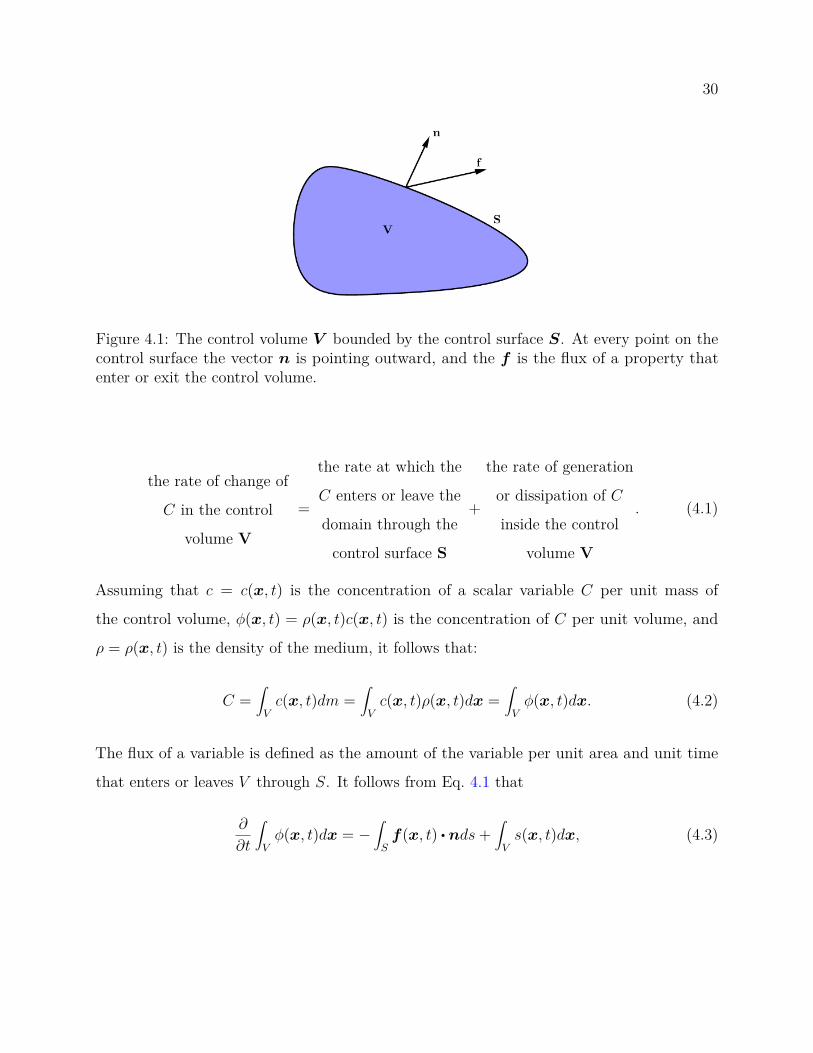
30
Figure 4.1: The control volume V bounded by the control surface S. At every point on thecontrol surface the vector n is pointing outward, and the f is the flux of a property thatenter or exit the control volume.
the rate of change of
C in the control
volume V
=
the rate at which the
C enters or leave the
domain through the
control surface S
+
the rate of generation
or dissipation of C
inside the control
volume V
. (4.1)
Assuming that c = c(x, t) is the concentration of a scalar variable C per unit mass of
the control volume, φ(x, t) = ρ(x, t)c(x, t) is the concentration of C per unit volume, and
ρ = ρ(x, t) is the density of the medium, it follows that:
C =∫Vc(x, t)dm =
∫Vc(x, t)ρ(x, t)dx =
∫Vφ(x, t)dx. (4.2)
The flux of a variable is defined as the amount of the variable per unit area and unit time
that enters or leaves V through S. It follows from Eq. 4.1 that
∂
∂t
∫Vφ(x, t)dx = −
∫Sf(x, t) • nds+
∫Vs(x, t)dx, (4.3)

31
which is the integral form of conservation law. After applying the divergence theorem
∫Sf • nds =
∫V
(∇ • f)dx, (4.4)
and assuming that the functions φ(x, t) and f(x, t) are differentiable and the divergence
theorem holds, the differential form of the conservation law is obtained as follows,
∂φ(x, t)∂t
+∇ • f(x, t)− s(x, t) = 0. (4.5)
The flux of φ comes from advection and diffusion of φ as follows:
f(x, t) = u(x, t)φ(x, t)︸ ︷︷ ︸advection of φ
−D(x, t)∇φ(x, t)︸ ︷︷ ︸diffusion of φ
, (4.6)
where D is the diffusion matrix. Substituting the flux in Eq. 4.5 and dropping the space and
time dependency for simplicity, the following general form of conservation law is obtained:
∂φ
∂t+∇ • (uφ−D∇φ)− s = 0. (4.7)
4.1.1 Mass Conservation
Assume that c = 1, i.e. C is a scalar specifying the concentration of mass, and the integral
in Eq. 4.2 is the physical mass of the control volume. Substituting the φ = ρc = ρ in Eq. 4.5
and assuming the advective flux vector of f = uφ = ρu and no mass source (s = 0) leads to
the generic forms of the continuity equation:
∂ρ
∂t+∇ • (ρu) = 0, (4.8a)
∂ρ
∂t+ u • ∇ρ+ ρ∇ • u = 0, (4.8b)
Dρ
Dt+ ρ∇ • u = 0. (4.8c)

32
The last equation is derived after incorporating the material derivative,
D( )Dt
= ∂( )∂t
+ u • ∇( ). (4.9)
Incompressible flow assumption (Dρ/Dt = 0) may further simplify the mass conservation
equations Eqs. 4.8 to:
∇ • u = 0. (4.10)
4.1.2 Momentum Conservation
The conservation of momentum, also called Navier-Stokes equations, can be derived assuming
that c = u and φ = ρc = ρu, i.e. C is a vector specifying the momentum concentration. The
flux tensor can be written as the sum of advective and stress flux, i.e.
f =u(x, t)φ(x, t)− σ(x, t) = ρuu− σ
=ρ
u1u1 u1u2 u1u3
u2u1 u2u2 u2u3
u3u1 u3u2 u3u3
+
σ11 σ12 σ13
σ21 σ22 σ23
σ31 σ32 σ33
, (4.11)
where uu is a tensor results from the dyadic product of u by itself, and σ(x, t) is the stress
flux. Substituting the flux tensor of Eq. 4.11 in Eq. 4.5 results in the conservative Cauchy
equations as follows
∂(ρu)∂t
+∇ • (ρuu− σ)− s = 0, (4.12)
Further simplifications to the advective flux is possible assuming an incompressible flow.
After incorporating the mass conservation ∇ • u = 0 and using the following identity
∇ • (uφ) = u • ∇φ+ φ∇ • u, (4.13)
33
with φ = ρu the second term can be simplified to
∇ • (ρuu) = u • ∇(ρu) + ρu(∇ • u) = u • ∇(ρu), (4.14)
which subsequently can be used in conjunction with 4.9 to express the Cauchy equation in
Lagrangian form as follows:
D(ρu)Dt
−∇ • σ − s = 0. (4.15)
Note that Eq. 4.14 simplifies the equations for a divergence-free velocity field. However, if
the initial velocity field is not divergence-free, there will be error associated with ignoring
this term at the initial time step.
Eqs. 4.12 and 4.15 are respectively Eulerian and Lagrangian momentum transport in
any continuum. Further simplification requires more information about the nature of the
continuum of interest. Conventionally in fluids and many other incompressible continua, σ
can be decomposed into a volumetric (hydrostatic) part and a traceless deviatoric part, as
follows:
σ = σdev + σvol, (4.16)
tr(σvol) = tr(σ) = σ11 + σ22 + σ33, (4.17)
tr(σdev) = 0. (4.18)
where tr() indicates sum of the diagonal elements of a tensor. Defining
p = −(σ11 + σ22 + σ33)/3, (4.19)
to be the mechanical pressure, the volumetric and the deviatoric parts of the stress tensor

34
may be written as follows:
σvol = (σ : I3 )I = (σ11 + σ22 + σ33
3 )I = −p
1 0 0
0 1 0
0 0 1
, (4.20)
σdev = σ − (σ : I3 )I =
σ11 σ12 σ13
σ21 σ22 σ23
σ31 σ32 σ33
+
p 0 0
0 p 0
0 0 p
. (4.21)
Ultimately, substituting the flux of Eq. 4.11 and stress decomposition of Eqs. 4.16, 4.20 and
4.21 into Eq. 4.5 leads to:
∂ρu
∂t+∇ • (ρuu− σvol − σdev)− fb = 0, (4.22)
where fb is the body force that acts as the source term s seen in 4.5. According to
∇ • (−σvol) = ∇ • (pI) = ∇p, (4.23)
the momentum conservation for Eulerian frameworks becomes:
∂(ρu)∂t
+ u • ∇(ρu) +∇p−∇ • σdev − fb = 0. (4.24)
After applying the material derivative (Eq. 4.9), the Lagrangian form of the momentum
equation is obtained as follows:
D(ρu)Dt
+∇p−∇ • σdev − fb = 0. (4.25)

35
4.2 Material Modeling
The momentum balance equations described in Eqs. 4.24 and 4.25 express fewer equations
than unknowns (p,u,σ) for a general continuum. Hence, material behavior may be used to
introduce more equations for closure. In the following section, constitutive equations required
for modeling the ∇ • σdev term for the continua of interest in this work are presented.
4.2.1 Newtonian Model
For Newtonian fluids, the deviatoric part of the stress tensor is related to the shear rate,
through σdev = 2µE, where µ is a constant representing the dynamic viscosity of the fluid
and deformation-rate tensor E is obtained from the velocity gradient tensor as follows,
E = 12(∇u +∇uT). (4.26)
Above note that E is half of the strain-rate tensor, (∇u + ∇uT). Given that ∇ • u = 0
for incompressible flows, the term ∇ • σdev may be simplified using the incompressible flow
assumption as follows:
∇ • σdev = ∇ • (µ(∇u +∇uT))
= µ∇ • (∇u) + µ∇(∇ • u)
= µ∇2u, (4.27)
where
∇2 = ∂2
∂x2 + ∂2
∂y2 + ∂2
∂z2 . (4.28)
36
is the Laplacian operator. Above, note that divergence of a second-order tensor S is defined
via ∇ • σ = σki,iek as follows:
∇ • S = [ ∂∂x,∂
∂y,∂
∂z] •
S11 S12 S13
S21 S22 S23
S31 S32 S33
=
∂S11
∂x+ ∂S12
∂y+ ∂S13
∂z
∂S21
∂x+ ∂S22
∂y+ ∂S23
∂z
∂S31
∂x+ ∂S32
∂y+ ∂S33
∂z
. (4.29)
Furthermore, given that ∇u = ∇(uiei) = (uiei),jej = ui,jeiej, the velocity gradient tensor
and its transpose are defined as follows
∇u = ∇
u1
u2
u3
=
∂u1
∂x
∂u1
∂y
∂u1
∂z
∂u2
∂x
∂u2
∂y
∂u2
∂z
∂u3
∂x
∂u3
∂y
∂u3
∂z
, (4.30)
∇uT =
∂u1
∂x
∂u2
∂x
∂u3
∂x
∂u1
∂2∂u2
∂y
∂u3
∂x
∂u1
∂3∂u3
∂z
∂u3
∂x
. (4.31)
The final form of the momentum conservation described in Eqs. 4.24-4.25 under incom-
pressible flow assumption and Newtonian fluid model is then:
∂ρu
∂t+ u • ∇(ρu) +∇p− µ∇2u− fb = 0, (4.32a)
D(ρu)Dt
+∇p− µ∇2u− fb = 0, (4.32b)
where Eq. 4.32a is used in Eulerian frameworks and Eq. 4.32b is the Lagrangian counterpart
37
obtained after condensing the first two terms of Eq. 4.32a via the material derivative relation
(Eq. 4.9).
The adimensionalized Navier-Stokes equations may be written as follows:
Dudt
= −Eu∇pρ
+ 1Re∇2u + 1
Fr2 f b , (4.33)
where the Euler number, Eu = p0ρ0u2
0, is the ratio of the pressure to inertia forces (or static
pressure to dynamic pressure). The Reynolds number, Re = ρu0L0µ
, may be seen as the
ratio of inertia to viscous forces. Finally, the Froude number, Fr = U0√g0L0
, may be seen
as the ratio of the inertia to body forces. From the inviscid fluid assumption made in this
paper, µ = 0, the 1Re∇2u term drops out of the equations and the momentum balance is the
interplay of inertia, pressure and gravity/body force. In other words, the equations come
down to the conservative Euler equations, where the relative significance of different terms
are characterized by the magnitude Fr and Eu numbers.
4.2.2 Non-Newtonian Model
Contrary to Newtonian fluids where the viscosity is a constant, in non-Newtonian fluid models
it depends on parameters such as yield stress, shear-rate, and so forth. Many models have
been propose to capture shear thinning, shear-thickening, and yield stress. Amongst all
the possible fluid models, the Herschel-BulklManey fluid is employed in the present work.
Defining the shear stress and shear strain-rate from their underlying tensors, respectively
according to
τ =√
2σdevij : σdevij (4.34)
γ =√
2Eij : Eij , (4.35)
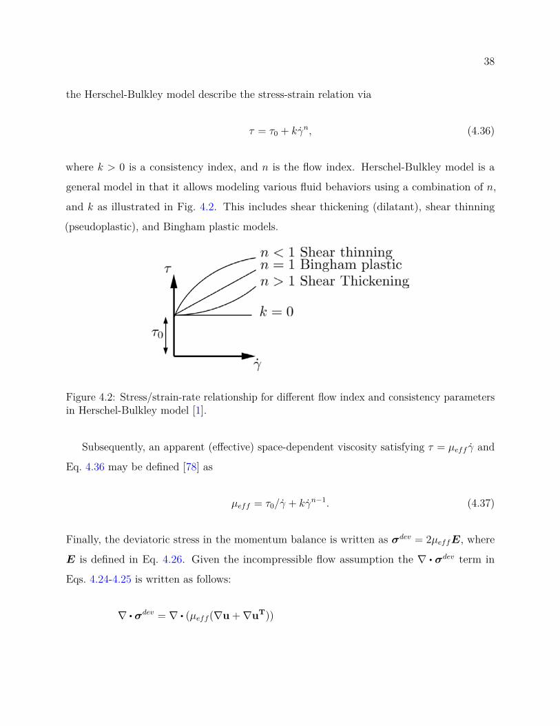
38
the Herschel-Bulkley model describe the stress-strain relation via
τ = τ0 + kγn, (4.36)
where k > 0 is a consistency index, and n is the flow index. Herschel-Bulkley model is a
general model in that it allows modeling various fluid behaviors using a combination of n,
and k as illustrated in Fig. 4.2. This includes shear thickening (dilatant), shear thinning
(pseudoplastic), and Bingham plastic models.
Figure 4.2: Stress/strain-rate relationship for different flow index and consistency parametersin Herschel-Bulkley model [1].
Subsequently, an apparent (effective) space-dependent viscosity satisfying τ = µeff γ and
Eq. 4.36 may be defined [78] as
µeff = τ0/γ + kγn−1. (4.37)
Finally, the deviatoric stress in the momentum balance is written as σdev = 2µeffE, where
E is defined in Eq. 4.26. Given the incompressible flow assumption the ∇ • σdev term in
Eqs. 4.24-4.25 is written as follows:
∇ • σdev = ∇ • (µeff (∇u +∇uT))

39
= µeff∇ • (∇u) +∇µeff • ∇u+ µeff∇(∇ • u) +∇µeff • ∇uT
= µeff∇2u+∇µeff • (∇u+∇uT ). (4.38)
The final form of the momentum balance for non-Newtonian fluids in Eulerian and Lagrangian
frameworks respectively is as follows:
∂ρu
∂t+ u • ∇(ρu) +∇p− µeff∇2u−∇µeff • (∇u+∇uT )− fb = 0, (4.39a)
D(ρu)Dt
+∇p− µeff∇2u−∇µeff • (∇u+∇uT )− fb = 0. (4.39b)
4.2.3 Granular Material
Proper continuum rheological models allows for applying Eqs. 4.24 and 4.25 to granular
materials. Amongst those, the µ(I) rheology [79] and the three-dimensional extension proposed
in [67] have been applied successfully in many works. The non-local rheology proposed in
[80] improves the rate-independent Drucker-Prager and Mohr-Coulomb model for dense and
rapid granular flows.
In the present work, a rigid-plastic assumption is made. This assumption neglects the
elastic response of the grains and approximates all flow as plastic flow. A similar strategy was
employed in an Eulerian framework in [81]. Another fundamental assumption made herein is
to neglect the small variation of the volume fraction observed in the dense regime and describe
granular material as an incompressible fluid [67, 82]. Following the stress decomposition
described in Eqs. 4.16, 4.19, 4.20, and 4.21, the deviatoric part of the stress tensor in the
momentum balance Eq. 4.25 is written similar to the non-Newtonian fluid model described
in §4.2.2 as
σdev = 2µeffE, (4.40)
where E is defined in Eq. 4.26. This assumption about the codirectionality of the stress

40
and strain-rate tensors neglects the presence of anisotropy that causes the eigenvectors of
stress and strain-rate to misalign [82]. The effective viscosity of granular material has been
described via
µeff = µgp
γ, (4.41)
in many previous works [67], where µg is used to denote the granular material friction
coefficient, and γ and p are defined from Eqs. 4.35 and 4.19, respectively. Subscript g is used
to distinguish the friction coefficient in granular medium, µg, from the fluid viscosity µ.
The aforementioned description of the µeff is a special variance of the non-Newtonian
model described by Eq. 4.37,
µeff = τ0/γ + kγn−1,
for k = 0 and τ0 = µgp. The choice of µgp for the yield stress τ0 stands to the following
rational. Consider the mass-spring-damper system shown in Fig. 4.3. Writing the force
balance for the system as
mx = −kx+−cx− µgFn, (4.42)
and dividing both sides by the contact area A, it follows that:
m
Ax =− k
Ax+− c
Ax− µg
FnA,
m
Ax =− k′x︸︷︷︸
Elasticity
− c′x︸︷︷︸Viscosity
− µgp︸︷︷︸Frictional contact
. (4.43)

41
k
cm µg, A
x
Fn = p A
Figure 4.3: A mass-spring-damper system consisting of viscous, elastic, and frictional resistiveforces.
Accordingly, the relationship between elastic, viscous and frictional stresses may be seen
as follows. The viscous stress is related to rate of deformation (c′x and Eq. 4.40), while
frictional contact causes a yield stress below which no motion happens. Hence, the choice of
τ0 = µgp in Eq. 4.37 (see also Fig. 4.2) is justified. Thus, the continuum modeling of granular
material is performed as a special case of non-Newtonian fluids.
4.3 Time Integration
In this section the main ideas behind the time integration of the continuum equations discussed
in previous sections are described. The time-integration discussed herein are not tied to the
choice of space discretization and are common among various Eulerian and Lagrangian CFD
solvers. These integration schemes are employed in the I2SPH method that will be described
in section §4.4.3.
4.3.1 Projection Method
This algorithm is based on the Helmholtz-Hodge decomposition, which states that any vector
field u may be decomposed into a solenoidal (usol) and an irrotational (uirrot) part as follows:
u = uirrot + usol, (4.44)

42
where the solenoidal part is divergent-free (∇.usol = 0). The irrotational part is curl-free
(∇× uirrot=0) and can be written as the gradient of a potential/scalar field (uirrot = ∇φ).
The irrotational part is a conservative vector field, and the line integral of this field is path-
independent. By taking divergence of u and using the divergent-free property of usol, it can
be seen that
∇ • u = ∇ • uirrot = ∇2φ, (4.45)
and given that u is known, the Poisson equation 4.45 can be solved for φ which finally results
in usol = u− uirrot = u−∇φ.
In a similar fashion, we can decompose the force field per unit mass (DuDt
) of Equation
4.32b into a solenoidal field (ν∇2u+ fb) and an irrotational field (−1ρ∇p). The semi-discrete
form (discretized only in time) of Eq. 4.32b is written as follows:
(un+1 − un)∆t = (un+1 − u∗)
∆t︸ ︷︷ ︸solenoidal contribution
+ (u∗ − u)∆t︸ ︷︷ ︸
irrotational contribution
= −1ρ∇p+ ν∇2un + g. (4.46)
4.3.2 Non-Incremental Projection Method
Based on the previous discussion the following decomposition is conducted:
(u∗ − un)∆t = + ν∇2un + g = fn x ∈ Ω, u∗ = 0 x ∈ ∂Ω, (4.47)
(un+1 − u∗)∆t =− 1
ρ∇pn+1 x ∈ Ω, ∇.un+1 = 0 ∈ ∂Ω. (4.48)
Eq. 4.47 is the predictor step and it can be used to find the intermediate velocity u∗:
u∗ = fn∆t+ un. (4.49)
Moreover, if pressure is known, Eq. 4.48 may be used to find un+1 as follows
un+1 = −∆t1ρ∇pn+1 + u∗. (4.50)
43
In order to obtain the pressure equation, using the approach led to Eq. 4.45, we take divergence
of the Eq. 4.48 and obtain the Poisson equation for pressure.
∇ • un+1 −∇ • u∗
∆t = −1ρ∇2pn+1. (4.51)
Note that from continuity Eq. 4.8a with incompressible flow assumption Dρ
Dt= 0 we can
write ∇ • un+1 = 0 and simplify Eq. 4.51 to
1ρ∇2pn+1 = ∇
• u∗
∆t , ∇pn+1 • n|∂Ω = 0. (4.52)
Next, Eq. 4.50 is used to update the velocities. The algorithm described above, velocity-based
projection, is usually preferred when the density variation is small and DρDt
= 0 holds. For
Lagrangian methods such as SPH, when working with free-surface flows, the density-based
projection method is considered to be more accurate. In this method, the continuity equation
is used to replace the velocity divergence term ∇• u∗
∆t in Eq. 4.52. The semi-discrete continuity
equation is as followsρ∗ − ρn
∆t = −ρn∇ • u∗. (4.53)
Using the right hand side of 4.53, one may write Eq. 4.52 as follows:
1ρ∇2pn+1 = − 1
ρnρ∗ − ρn
∆t2 , (4.54)
which takes into consideration the density variation as a source term in the Poisson equation.
Another important aspect of the discretization of Eq. 4.47 has to do with the treatment of
the viscous forces. This discretization may be chosen to be explicit, implicit or semi-implicit
in terms of u∗ as follows:
(u∗ − un)∆t = +ν(θ∇2u∗ + (1− θ)∇2un) + g = fn. (4.55)

44
Eq. 4.55 corresponds to the fully-explicit scheme (E 4.47) for θ = 0, and to fully-implicit
scheme for θ = 1. Crank-Nicolson discretization is obtained via θ = 0.5.
4.3.3 Incremental Projection Method
The incremental projection method with the Crank-Nicolson correction applied to the predic-
tion step is as follows:
(u∗ − un)∆t =ν2(∇2u∗ +∇2un)− 1
ρ∇p+ g = fn, (4.56)
(un+1 − u∗)∆t =− 1
ρ(∇pn+1 −∇pn) = −1
ρ(∇φ), (4.57)
φ =pn+1 − pn. (4.58)
Herein, the Poisson equation is solved for φ instead of pn+1. On an Eulerian grid, the pressure
correction is performed via pn+1 = pn + φ, whereas in the Lagrangian methods the pressure
correction is as follows:
pn+1 = pn + φ+∇pn+1 • (xn+1 − xn). (4.59)
See [83, 84] for more details about the advantages of the incremental projection method over
the non-incremental variation.
4.4 Space Discretization
Given the problems of interest in the present work, we choose to employ a Lagrangian
discretization method for spatial discretization of the governing equations of continua (Eqs. 4.8
and 4.25). Amongst possible choices of the Lagrangian methods, we choose the Smoothed
Particle Hydrodynamics method as it has been studied quite extensively in the literature for
the Navier-Stokes equations.

45
4.4.1 Smoothed Particle Hydrodynamics
The SPH approximation of a function f at location ri as [18]
f(ri) ≈ 〈f〉i =∑j∈S(i)
mj
ρjf(rj)Wij , (4.60)
where 〈f〉i indicates the SPH approximation of f at the location of SPH particle, or marker,
i; S(i) represents the collection of SPH particles found in the support domain associated
with particle i; ρj is the density ρ(rj) at location rj of particle j; mj = ρjVj and Vj =
(∑k∈S(j) Wjk)−1 are the mass and volume associated with marker j, respectively; Wij ≡
W (|ri − rj|, h), where |r| is the length of r. The kernel function W can assume various
expressions, e.g., a cubic spline kernel for 3D problems:
W (|r|, h) = 514πh3 ×
(2− q)3 − 4(1− q)3, 0 ≤ q < 1
(2− q)3, 1 ≤ q < 2
0, q ≥ 2
, (4.61)
where, if the kernel function is located at the origin, q ≡ |r|/h. The radius of the support
domain, κh, is proportional to the characteristic length h through the parameter κ, the latter
commonly set to 2 for the cubic spline kernel as shown in Fig. 4.4.
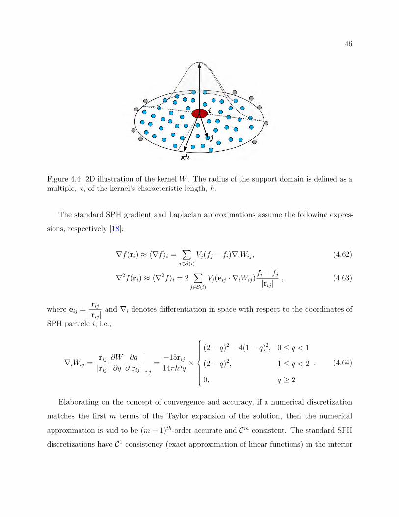
46
Figure 4.4: 2D illustration of the kernel W . The radius of the support domain is defined as amultiple, κ, of the kernel’s characteristic length, h.
The standard SPH gradient and Laplacian approximations assume the following expres-
sions, respectively [18]:
∇f(ri) ≈ 〈∇f〉i =∑j∈S(i)
Vj(fj − fi)∇iWij, (4.62)
∇2f(ri) ≈ 〈∇2f〉i = 2∑j∈S(i)
Vj(eij · ∇iWij)fi − fj|rij|
, (4.63)
where eij = rij|rij|
and ∇i denotes differentiation in space with respect to the coordinates of
SPH particle i; i.e.,
∇iWij = rij|rij|
∂W
∂q
∂q
∂|rij|
∣∣∣∣∣i,j
= −15rij14πh5q
×
(2− q)2 − 4(1− q)2, 0 ≤ q < 1
(2− q)2, 1 ≤ q < 2
0, q ≥ 2
. (4.64)
Elaborating on the concept of convergence and accuracy, if a numerical discretization
matches the first m terms of the Taylor expansion of the solution, then the numerical
approximation is said to be (m+ 1)th-order accurate and Cm consistent. The standard SPH
discretizations have C1 consistency (exact approximation of linear functions) in the interior

47
of the domain provided a regular particle distribution is maintained. If the particle regularity
is lost over time, the standard discretization is no longer C1 consistent and corrections are
required in order to maintain the consistency order. However, once the kernel function is
altered to retain consistency, the SPH discretization will forfeit its symmetry attributes thus
losing its conservation trait. Whereas conservative schemes are essential for the discretization
of the pressure gradient term and pressure-driven flows, consistent schemes play a more
important role in viscous flows. One side effect of using a consistent discretization is that
it requires smaller kernel support [28, 29]. Reducing the support size and thus the number
of neighbors is more critical in implicit solvers since linear system fill-in is dictated by the
number of SPH particle neighbors. This is the rationale for using a consistent formulation
for the implicit SPH method discussed herein, see §4.4.3, whenever handling an interior flow
scenario.
The “consistent” discretization already defined for the conservative case in Eqs. 4.62 and 4.63
assumes the expression [25, 27]
∇f(ri) ≈ 〈∇f〉i =∑j∈S(i)
Vj(fj − fi) Gi ∇iWij, (4.65)
∇2f(ri) ≈ 〈∇2f〉i = 2∑j∈S(i)
[Li : (eij ⊗∇iWij)]fi − fj|rij|
− eij · ∇fi
Vj, (4.66)
where “⊗" represents the dyadic product of the two vectors; “:" represents the double dot
product of two matrices; and Gi and Li are second-order, symmetric correction tensors. The
(m,n) element of the inverse of Gi is expressed as [26, 27, 25]:
(G−1i )mn = −
∑j
rmij∇i,nWijVj . (4.67)
The 3× 3 matrix Li is symmetric and has six unknowns obtained as the solution of a linear
system [25]. The required six independent equations may be obtained by expanding the
following equation for the upper/lower triangular elements of a 3× 3 matrix, e.g. m = 1, n =
48
1, 2, 3, m = 2, n = 2, 3, and m = 3, n = 3.
−δmn =∑j
(Akmni ekij + rmij enij)(L
opi e
oij∇i,pWijVj) , (4.68)
where δmn is the Kronecker symbol, and the elements of the third order tensor Ai are obtained
as
Akmni =∑j
rmij rnijG
kqi ∇i,qWijVj . (4.69)
A detailed account of obtaining the elements Li is provided in [85].
The outcome of the SPH discretization steps described above can be conveniently repre-
sented in matrix form. To that end, at the beginning of a time step one computes and stores
the discretization matrices AG and AL that arise from either the standard discretization
Eqs. 4.62-4.63, or the consistent discretization of Eqs. 4.65-4.66. For instance, working with
Eq. 4.63, 〈∇2f〉i can be expressed as follows:
〈∇2f〉i = ALi f , (4.70)
f =[f1 f2 · · · fP
]T, (4.71)
ALi =
[· · · , 2∑j∈S(i) Vj(eij · ∇iWij) 1
|rij |︸ ︷︷ ︸ith element
, · · · , −2Vj(eij · ∇iWij) 1|rij |︸ ︷︷ ︸
jth element s.t. j∈S(i)
, · · ·], (4.72)
where the subscript P denotes the number of SPH particles in the domain. Similarly, the
gradient of a scalar field 〈∇f〉i and divergence of a vector field 〈∇.u〉i may be computed from
Eq. 4.62 as follows:
〈∇f〉i =
AGxi
AGyi
AGzi
f , (4.73)
〈∇ · u〉i = AGxi ux + AGy
i uy + AGzi uz, (4.74)

49
f =[f1, f2, · · · , fP
]T, (4.75)
ux =[(ux)1, (ux)2, · · · , (ux)P
]T, (4.76)
uy =[(uy)1, (uy)2, · · · , (uy)P
]T, (4.77)
uz =[(uz)1, (uz)2, · · · , (uz)P
]T, (4.78)
where
AGxi =
[· · · , −∑j∈S(i) Vj∇i,1Wij, · · · , Vj∇i,1Wij, · · ·
], (4.79)
AGyi =
[· · · , −∑j∈S(i) Vj∇i,2Wij, · · · , Vj∇i,2Wij, · · ·
], (4.80)
AGzi =
[· · · , −∑j∈S(i) Vj∇i,3Wij, · · · , Vj∇i,3Wij, · · ·
], (4.81)
AGi =
[· · · , −∑j∈S(i) Vj∇iWij︸ ︷︷ ︸
ith element
, · · · , Vj∇iWij︸ ︷︷ ︸jth element s.t. j∈S(i)
, · · ·]. (4.82)
The same approach can be used to obtain the discretization matrices for the consistent
discretization of Eqs. 4.65-4.66. The system level matrices AG and AL are obtained as
〈∇f〉x =
〈∇f〉x1
〈∇f〉x2...
〈∇f〉xP
= AGxf , 〈∇f〉y =
〈∇f〉y1
〈∇f〉y2...
〈∇f〉yP
= AGyf , 〈∇f〉z =
〈∇f〉z1
〈∇f〉z2...
〈∇f〉zP
= AGzf ,
(4.83)
〈∇ · u〉 =[〈∇ · u〉1, 〈∇ · u〉2, · · · , 〈∇ · u〉P
]T= AGxux + AGyuy + AGzuz, (4.84)
50
AGx =
AGx1
AGx2
...
AGxP
, AGy =
AGy1
AGy2
...
AGyP
, AGz =
AGz1
AGz2
...
AGzP
, (4.85)
〈∇2f〉 = ALf , (4.86)
〈∇2f〉 =[〈∇2f〉1, 〈∇2f〉2, · · · , 〈∇2f〉P
]T, (4.87)
AL =
AL1
AL2
...
ALP
. (4.88)
This allows for the space discretization of the incompressible Navier-Stokes equations in the
x, y, and z directions, per Eq. 4.32b,
dux
dt≈ −1
ρAGxp + νALux + f bx
duy
dt≈ −1
ρAGyp + νALuy + f by
duz
dt≈ −1
ρAGzp + νALuz + f bz
, (4.89)
where
p =[p1, p2, · · · , pP
]T, (4.90)
is the vector of pressures and and ux, uy, and uz were defined in Eq. 4.78.

51
4.4.1.1 Particle Shifting
The advection of SPH particles can lead to scenarios characterized by high particle disorder
and/or regions with high particle depletion/plenitude. Maintaining the accuracy and stability
of the SPH method under these circumstances requires mitigating measures, one being particle
shifting. The latter calls for retiring a particle only to introduce it back in a consistent
fashion, slightly away from the previous location and the streamlines in order to improve
the uniformity of the SPH particle distribution. Particle shifting in conjunction with an
ISPH-type implementation was used in [86] and subsequently reported to be effective in
[28]. It has also been used in conjunction with a WCSPH-class implementation in [87]. The
shifting vector is computed for particle i as
δri = βr20umax∆t
∑j∈S(i)
rijr3ij
,
where r0 = 1Ni
∑jrij, umax is the maximum velocity in the domain, ∆t is the integration
time step, and β is an adjustable dimensionless parameter determining the magnitude of
the shifting vector. At the end of each time step the position of particle i is shifted by
xnewi = xi + δri. Accordingly, the field variable ρi, pi, and vi are updated as
pnewi = pi +∇pi · δri , ρnewi = ρi +∇ρi · δri , and unewi = ui +∇ui · δri .
4.4.2 WCSPH
The cornerstone of WCSPH is its use of a state equation to obtain the pressure from density
– at marker i,
pi = (k|u|max)2( ρiρ0− 1
)+ p0 , (4.91)
where k|u|max is a sound speed proxy; |u|max is the magnitude of the maximum velocity in
the domain; k = 10 is an empirical scaling factor; and ρ0 and p0 are reference values. The
density update may be obtained from the time integration of the continuity equation Eq. 4.8
52
using the space discretization of the velocity divergence from Eq. 4.84
ρn+1 − ρn
∆t = − < ρn • (AGxux + AGyuy + AGzuz) > , (4.92)
where ρn ≡[ρ0, ρ1, · · · , ρP
]Tis the system level vector of markers’ density at the current
time step, and c =< a · b > indicates the element-wise product of vector a and b. The time
integration used is of predictor-corrector type:
predictor stage:
un+1/2 = un + ∆t
2 an
xn+1/2 = xn + ∆t2 un
,
and
corrector stage:
un+1/2 = un + ∆t
2 an+1/2
xn+1/2 = xn + ∆t2 un+1/2
.
Finally,
update stage:
un+1 = 2un+1/2 − un
xn+1 = 2xn+1/2 − xn.
Above, an is the system-level vector of accelerations at time step n; its components in the x,
y, z directions are obtained from the space discretization of the Navier-Stokes as
(ax)n = −1ρ(AGx)npn + ν(AL)nunx + f bx
(ay)n = −1ρ(AGy)npn + ν(AL)nuny + f by
(az)n = −1ρ(AGz)npn + ν(AL)nunz + f bz
.

53
Likewise, an+1/2 in the corrector stage is obtained using xn+1/2, un+1/2, and the associated
discrete representation of the gradient and Laplacian operators, i.e. (AG)n+1/2, and (AL)n+1/2.
As far as the time step ∆t is concerned, its size is constrained on numerical stability grounds
by the following condition [88]:
∆t ≤ min
0.25 h
k|v|max, 0.125h
2
ν, 0.25
√h
|fb|
. (4.93)
Above, the first term corresponds to the CFL condition and is the place where the “numerical
stiffness” of the state equation in Eq. 4.91 comes into play. Specifically, the higher the k value,
the lower the amount of allowed compressibility, and, at the same time, the smaller the time
step. The second restriction in Eq. 4.93 appears due to the explicit treatment of the viscous
term and restricts the time step by a factor that is inversely proportional to the viscosity –
the higher the viscosity, the lower the time step. More importantly, the second restriction
is also proportional to h2, which significantly and adversely impacts the time step when a
finer particle distribution is employed. The last restriction is due to the explicit treatment of
the external (body) forces. Ultimately, these relatively stringent bounds on the time step ∆t
prompted the search for alternative SPH-based approaches; e.g., ISPH and KCSPH.
4.4.3 ISPH
ISPH alleviates the time step constraints hindering WCSPH at the price of solving a linear
system of equations at each time step. It draws on the Helmholtz-Hodge decomposition and
Chorin’s projection method [89] to integrate the continuity and the Navier-Stokes equation
as:
prediction:
(u∗ − un)
∆t = ν2 (∇2u∗ +∇2un) + f b x ∈ Ω
u∗ = 0 x ∈ ∂Ω, (4.94)
54
correction:
(un+1 − u∗)
∆t = −1ρ∇pn+1 x ∈ Ω
∇ • un+1 = 0. (4.95)
Equation 4.94 is the predictor step used to find the intermediate velocity u∗. Taking divergence
of the Eq. 4.95, the Poisson equation for pressure may be obtained as follows:
∇ • un+1 −∇ • u∗
∆t = −1ρ∇2pn+1. (4.96)
The incompressible flow assumption, ∇.un+1 = 0, can be used to simplify Eq. 4.96 to
1ρ∇2pn+1 = ∇
• u∗
∆t∇pn+1 • n|∂Ω = 0
. (4.97)
Once the above Poisson problem is solved for pressure, Eq. 4.95 may be used to find un+1 as
un+1 = −∆t1ρ∇pn+1 + u∗ .
The algorithm described above is known as the velocity-based projection version. However,
when working with free-surface flows, it is beneficial to use a density-based projection method
[90] to account for the density variation experienced by the SPH particles in the proximity of
the free surface. The continuity equation is then used to replace the velocity divergence term∇.u∗
∆t in Eq. 4.97. The semi-discrete continuity equation corresponding to the prediction state
is:ρ∗ − ρn
∆t = −ρn∇ • u∗. (4.98)
55
Using the right hand side of Eq. 4.98, one may write Eq. 4.97 as
1ρ∇2pn+1 = − 1
ρnρ∗ − ρn
∆t2
∇pn+1 • n|∂Ω = 0, (4.99)
which takes into consideration the density variation as a source term in the Poisson equation.
Following an approach similar to the one introduced in [90], we use a stabilization of the
source term in the Poisson equation to linearly combine the right-hand sides of Eqs. 4.97 and
4.99:
Pressure equation:
1ρ∇2pn+1 = α
1ρnρn − ρ∗
∆t2 + (1− α)∇• u∗
∆t∇pn+1 • n|∂Ω = 0
.
This stabilization technique turned out to be critical in simulations where the difference
between the density and the rest density (ρ0) is large.
The above time-discretized equations may be combined with the space-discretization of
Eqs. 4.83 and 4.86. The space-time discretized ISPH equations are as follows:
(1
∆tI−ν2AL
)u∗x =
(1
∆tI + ν2AL
)unx + f bx particles ∈ Ω(
1∆tI−
ν2AL
)u∗y =
(1
∆tI + ν2AL
)uny + f by particles ∈ Ω(
1∆tI−
ν2AL
)u∗z =
(1
∆tI + ν2AL
)unz + f bz particles ∈ Ω
u∗ = 0 on ∂Ω
, (4.100)
1ρALpn+1 = α
1ρnρn − ρ∗
∆t2 + (1− α)AGxu∗x + AGyu∗y + AGzu∗z
∆t∇pn+1 • n|∂Ω = 0
, (4.101)
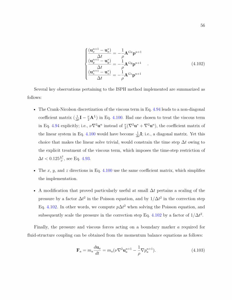
56
(un+1x − u∗x)
∆t = −1ρAGxpn+1
(un+1y − u∗y)
∆t = −1ρAGypn+1
(un+1z − u∗z)
∆t = −1ρAGzpn+1
. (4.102)
Several key observations pertaining to the ISPH method implemented are summarized as
follows:
• The Crank-Nicolson discretization of the viscous term in Eq. 4.94 leads to a non-diagonal
coefficient matrix ( 1∆tI−
ν2AL) in Eq. 4.100. Had one chosen to treat the viscous term
in Eq. 4.94 explicitly; i.e., ν∇2un instead of ν2 (∇2u∗ +∇2un), the coefficient matrix of
the linear system in Eq. 4.100 would have become 1∆tI; i.e., a diagonal matrix. Yet this
choice that makes the linear solve trivial, would constrain the time step ∆t owing to
the explicit treatment of the viscous term, which imposes the time-step restriction of
∆t < 0.125h2
ν, see Eq. 4.93.
• The x, y, and z directions in Eq. 4.100 use the same coefficient matrix, which simplifies
the implementation.
• A modification that proved particularly useful at small ∆t pertains a scaling of the
pressure by a factor ∆t2 in the Poisson equation, and by 1/∆t2 in the correction step
Eq. 4.102. In other words, we compute p∆t2 when solving the Poisson equation, and
subsequently scale the pressure in the correction step Eq. 4.102 by a factor of 1/∆t2.
Finally, the pressure and viscous forces acting on a boundary marker a required for
fluid-structure coupling can be obtained from the momentum balance equations as follows:
Fa = maduadt
= ma(ν∇2un+1a − 1
ρ∇pn+1
a ). (4.103)

57
4.4.4 IISPH
In the IISPH method of choice [14], the continuity equation, Eq. 4.8, is discretized in time
and space using forward Euler and the approximation in Eq. 4.62, respectively, to yield
ρi(t+ ∆t)− ρi(t)∆t =
∑j∈S(i)
mjvij(t+ ∆t) • ∇Wij , (4.104)
where ∆t is the time step. The Navier-Stokes equation, Eq. 4.32a, is discretized using Chorin’s
two-step projection method [89]. First, an intermediate velocity, denoted below by vnpij,l, is
obtained using the current state information to evaluate the velocities and the right-hand-side
terms of Eq. 4.32b except the pressure gradient term ∇p/ρ. Finally, new velocities are
obtained by correcting the intermediate velocity with pressure information at the new time
step. In IISPH, the pressure at the new time step is obtained by solving a Poisson equation.
The details are as follows. The solution methodology starts off by partitioning the forces in
the right-hand-side of the momentum equations:
mivi(tl + ∆t)− vi(tl)
∆t = f pi (tl + ∆t) + f np
i (tl) , (4.105)
where, in the light of Eq. 4.32a, f pi and f npi represent the pressure-related and non-pressure-
related forces acting on particle i, respectively. After simple manipulations,
vi,l+1 =(
vi,l +f npi,l
mi
∆t)
+f pi,l+1
mi
∆t = vnpi,l + vpi,l+1 , (4.106)
where vnpi,l ≡ vi,l + f npi /mi∆t is the intermediate velocity, vpi,l+1 ≡ f p
i,l+1∆t/mi is the velocity
correction, and subscripts l and l + 1 represent the discretized values at time tl and tl + ∆t,
respectively.
Unlike the original Chorin projection method and other incompressible SPH solutions,
which obtain the pressure equation by imposing the divergence-free velocity condition, i.e.
∇.v = 0, the pressure equation in IISPH is obtained by imposing dρ/dt = 0. The choice
58
of density-invariance condition leads to a more uniform particle distribution and a lower
density error whereas a divergence-free velocity condition results in a more accurate pressure
distribution [90]. Hence, in Eq. 4.104, the density is also divided into the pressure and
non-pressure parts. Subsequently, the intermediate density resulting from the intermediate
velocity vnpij,l is expressed as
ρnpi,l = ρi,l + ∆t∑j∈S(i)
mjvnpij,l∇Wij. (4.107)
Subtracting the above equation from Eq. 4.104 yields
ρi,l+1 − ρnpi,l = ∆t∑j∈S(i)
mj(vij,l+1 − vnpij,l)∇Wij . (4.108)
Incompressibility is enforced by setting ρi,l+1 = ρ0. Using Eq. 4.106 and the definition of
vpij,l+1, the above equation, after further manipulations, yields the pressure equation that is
formulated at the location of each particle i as
ρ0 − ρnpi,l = ∆t∑j∈S(i)
mjvpij,l+1∇Wij = ∆t2∑j∈S(i)
mj
f pi,l+1
mi
−f pj,l+1
mj
∇Wij , (4.109)
where the conservative pressure forces may be obtained from [14]
∆t2mi
f pi,l+1 =−∆t2
∑j∈S(i)
mj
(pi,l+1
ρ2i,l
+ pj,l+1
ρ2j,l
)∇Wij
=−∆t2
∑j∈S(i)
mj
ρ2i
∇Wij
︸ ︷︷ ︸
dii
pi,l+1 +∑j∈S(i)
(−∆t2mj
ρ2j
∇Wij
)︸ ︷︷ ︸
dij
pj,l+1
=diipi,l+1 +∑j∈S(i)
dijpj,l+1 ,
(4.110)

59
and the viscous force from [63]
f npi,l = mi
∑j∈S(i)
mjΠij + fb . (4.111)
Herein, fb represents the body force density and Πij ≡ −(µi + µj)xij∇Wij
ρ2ij(x2
ij + εh2ij)
vij,l, hij = (hi +
hj)/2 and ρij = (ρi + ρj)/2. Finally, by substituting Eqs. 4.107 and 4.110 into Eq. 4.8, a
linear system of equations, with pressure as the unknown, is obtained as follows:
ρ0 − ρnpi,l =∑j∈S(i)
mj
diipi,l+1 +∑t∈S(i)
ditpt,l+1 + djjpj,l+1 +∑
k∈S(j)djkpj,l+1
• ∇Wij
=pi,l+1
∑j∈S(i)
mj(dii − dji) • ∇Wij
︸ ︷︷ ︸
aii
+∑j∈S(i)
mj
∑t∈S(i)
ditpt,l+1 + djjpj,l+1 +∑
k∈S(j),k 6=idjkpj,l+1
• ∇Wij
=pi,l+1 aii +∑t∈S(i)
pt,l+1(dit •
∑j∈S(i)
mj∇Wij
)
+∑j∈S(i)
pj,l+1 mj djj • ∇Wij +∑j∈S(i)
mj
∑k∈S(j),k 6=i
djkpj,l+1 • ∇Wij.
(4.112)
Eq. 4.112 represents the pressure equation in the form of a linear system of equations, i.e.
Ap = b, where p =[p1, p2, p3, . . . , pNf
]T, b =
[ρ0 − ρnp1,l, ρ0 − ρnp2,l, ρ0 − ρnp3,l, . . . , ρ0 − ρnpNf
]T,
and Nf denotes the total number of SPH markers. Similarly, the elements of the sparse
matrix A can be obtained from Eq. 4.112. Once the pressure values are available, Eqs. 4.106
and 4.110 are used to compute the velocity at the new time step tl+1; subsequently, positions
are updated as xi,l+1 = xi,l + ∆t vi,l+1.
Unlike the weakly compressible SPH (WCSPH) algorithm invoked in the usual SPH
solution [18], the methodology described does not use a state equation. The highly oscillatory
60
nature of the solution (induced by the state equation) and the use of explicit integration
constrain WCSPH to small integration steps. Conveniently, the numerical method discussed
avoids the introduction of high frequency oscillations, which are a numerical artifact, and can
advance the solution at large integration time steps. Nevertheless, typical stability criteria
still hold. Herein, an adaptive time-stepping scheme is considered in which the time step ∆t
is constrained by the CourantFriedrichsLewy (CFL) condition, i.e. C = v∆t/h < Cmax, the
magnitude of volumetric forces |fb|, and the viscous dissipation [91, 92]:
∆t ≤ minCmaxhvmax
, 0.25 mini
( h
|fb|i) 1
2 , 0.125h2
ν , (4.113)
where subscript i denotes the particle i and Cmax depends on the integration scheme. In
the present study, Cmax < 0.1 was found to be sufficient for the stability of the numerical
solution. The solution methodology is outlined in Algorithm 1.
4.4.5 KCSPH
KCSPH approaches are relatively new and unconventional. They draw on a thermodynamically
consistent SPH discretization [93] that leads to an index 3 set of differential algebraic equations
(see Section 3.1 describing the motion of the fluid markers. The SPH particles can be regarded
as 3 degree-of-freedom point-masses constrained in their motion. Collectively, these kinematic
constraints capture the incompressibility of the fluid and couple the relative motion of the SPH
markers. Notably, the effect of these constraints comes into the momentum equations as well.
Indeed, the Lagrange multiplier forcing term that arises from the compressibility constraint
acts as the pressure gradient term in the momentum balance equations [93, 94, 95, 11].
The cornerstones of WCSPH and ISPH were, respectively, the use of a stiff state equation
for recovering the pressure, and the use of a Poisson equation to produce a pressure field that
enforces incompressibility. In KCSPH, the cornerstone is the use of holonomic kinematic
constraints to enforce incompressibility; i.e., one demands that at the location of marker i

61
Algorithm 1 Fluid Dynamics via IISPH1: for all particles i do2: Compute ρi,l =
∑j∈S(i) mjWij
3: end for4: Synchronize5: for all particles i do6: Calculate vnp
i,l and dii
7: end for8: Synchronize9: for all particles i do
10: Calculate ρnpi,l , aii, and cii =
∑j∈S(i) mj∇Wij
11: end for12: Synchronize13: for all fluid particles i do14: Set A(i, i) = aii15: if ρi,l > 0.99ρ0 then16: Set b(i) = ρ0 − ρnp
i,l
17: for all particles j ∈ S(i) do
18: A(i, j)+ = mj
(dij .cii + djj .∇Wij
)19: for all particles k ∈ S(j) do
20: A(i, k)+ = mj
(djk.∇Wij
)21: end for22: end for23: end if24: end for25: for all BCE particles i do26: Compute the prescribed wall velocity (vi,w) and acceleration (ai,w) at the position of marker i from the
motion of the associated deformable or rigid body. For rigid bodies they can be obtained from Eq. 3.7,and for deformable bodies from shape functions of Eqs. 3.23 and 3.2.2 along with the associated nodalgeneralized velocity and acceleration of the corresponding element.
27: The velocities of the BCE markers required for the no-slip conditions are obtained from Eq. 4.11928: Set vdummy = 0, den = 0 and29: for all fluid particles j ∈ S(i) do
30: b(i)+ = ρj
((g− aj,w) · rij
)Wij
31: Set A(i, j) = −Wij32: den+ = Wij and vdummy+ = vj,wWij33: end for34: if den < ε then35: vi = 2vi,w
36: A(i, i) = aii and b(i) = 037: else38: vi = 2vi,w − vdummy/den39: A(i, i) = den40: Scale all the elements of row i of A and b(i) by aii/den41: end if42: end for43: Solve Ap = b using BiCGStab or GMRES44: for all fluid particles i do
45: Correct velocities from vi,l+1 = vnpi,l +
f pi,l+1
mi∆t via Eq. 4.110
46: Update the state by xi,l+1 = xi,l + ∆t vi,l+147: end for

62
the density assumes a reference value ρ0:
Cfi = ρi − ρ0
ρ0= 0 . (4.114)
If the time-derivative of the constraints in Eq. 4.114 is satisfied at the velocity level, i.e.
Cfi = dρ/dt = 0, the following will emerge after applying Eq. 4.60; i.e., invoking the SPH
machinery:
Cfi = d
dt( ρiρ0− 1) ≈
∑j
mj
ρ0
dWij
dt=∑j
mj
ρ0
dWij
dxij.dxijdt
=∑j
mj
ρ0∇iWij.(ui − uj) = −
∑j
mj
ρ0∇iWij.(uj − ui) . (4.115)
Above, if ρj ≈ ρ0, the last term mimics − < ∇.u >i, see Eq. 4.62. Elements in row i of the
constraint Jacobian matrix ∇qg(q, t) ≡ G (see Eq. 3.4) are associated with the constraint
gi = Cfi = 0. These entries in G may be obtained via Eq. 4.115 as follows:
Cfi =
∑j
mj
ρ0∇iWijui −
∑j
mj
ρ0∇iWijuj
⇒ Gii = 1ρ0
∑k 6=i
mk∇Wik and Gij = −mj
ρ0∇iWij. (4.116)
Each density constraint on a marker contributes to a single row in the full Jacobian matrix
which has 3P columns. This matrix is sparse and its rows have three values at the columns
corresponding to the current marker i and three values for each marker j within the support
domain of i. More specifically, for row i
Gi =[· · · , 1
ρ0
∑j∈S(i) mk∇iW
Tik︸ ︷︷ ︸
ith element
, · · · , −mj
ρ0∇iW
Tij︸ ︷︷ ︸
jth element s.t. j∈S(i)
, · · ·]
1×3P. (4.117)
It is informative to compare Eqs. 4.117 and 4.82 to underline similarities between the
constraint Jacobian row Gi and the discretized gradient operator AGi . Qualitatively, the

63
density constraint Jacobian matrix is similar to the discretized gradient operator – satisfying
Gu = 0 is the analog of ∇.u = AGxux + AGyuy + AGzuz = 0 (see Eq. 4.74). This connection
between G and AG comes further into play when one considers how the pressure factors into
the Newton-Euler equations of motion. Imposing the kinematic constraint Cf = Gq = 0
leads to the presence of a Lagrange multiplier. The multipliers in Eq. 3.4 play a role similar to
that of the pressures. This becomes clearer when the force term associated with the Lagrange
multipliers in Eq. 3.4, i.e.(∇qg(q, t)
)TΛ is written as GTΛ, where the connection between
the G matrix and the discretized gradient matrix AG is considered. It follows that KCSPH
replaces the pressure gradient term −1ρAGp in the space-discretized Navier-Stokes (Eq. 4.89)
with GTΛ. Considering the resemblance of AG and the −G matrices, we may conclude
that the Lagrange multipliers scaled (element-wise) by the particles’ volume (Λ/V ) is the
mechanical pressure p in the Navier-Stokes equations.
Up to this point, the KCSPH discussion focused exclusively on obtaining the SPH equations
of motion in the form of Section 3.4’s differential-algebraic equations. In other words, the
spatial discretization step has been accomplished. How to discretize and solve in time these
differential-algebraic equations goes beyond the scope of this manuscript and the interested
reader is referred to [11].
4.4.6 Boundary Conditions
Herein, imposing boundary conditions (BCs) falls back on the use of so-called boundary
conditions enforcing (BCE) markers. These are fictitious markers, rigidly attached to the
boundary in a buffer zone that runs several layers of BCE markers deep. These markers
are used to enforce the no-slip and the no-penetration conditions, i.e., to satisfy the u∗ = 0
condition on the boundary. This condition is implemented differently in WCSPH, ISPH, and
KCSPH.
In one widely used approach [96], the expected kinematic attributes of the markers,
calculated from the motion of the solid phase at the location occupied by the markers, are
64
different from their assigned values. The latter are calculated such that the no-slip and
no-penetration boundary conditions are implicitly enforced at the fluid-solid interface. The
no-slip condition states that the velocity of the BCE markers should oppose the velocity of
the fluid particles such that the average relative fluid-solid velocity at the interface is zero;
i.e., the average velocity at the interface is the expected interface velocity. Herein, the induced
velocity ua at the position of marker a is computed from the velocity of the fluid markers as
ua =
∑b∈F
ubWab∑b∈F
Wab
, (4.118)
where F denotes a set of fluid markers that are within the compact support of the BCE
marker a. The no-slip condition holds if (ua + ua)/2 = upa; in other words the assigned
velocity of marker a is [96]:
ua = 2upa − ua , (4.119)
where upa is the expected wall velocity at the position of the marker a, and ua is an extrapolation
of the smoothed velocity field of the fluid phase to the BCE markers.
The pressure of a BCE marker may be calculated via a force balance condition at the
wall interface, which leads to [96]
pa =
∑b∈F
pbWab + (g− apa) •∑b∈F
ρbrabWab∑b∈F
Wab
, (4.120)
where g is the gravitational acceleration and apa is the acceleration of the boundary/solid at
the location of BCE marker a.
This approach is fairly straightforward to implement in WCSPH – one can modify the
velocity and pressure of the BCE markers according to Eqs. 4.119 and 4.120, respectively. In
regard to the ISPH method, (i) the no-slip boundary condition is implemented in the linear
system of Eq. 4.100; and, (ii) pressure boundary conditions should be incorporated into the
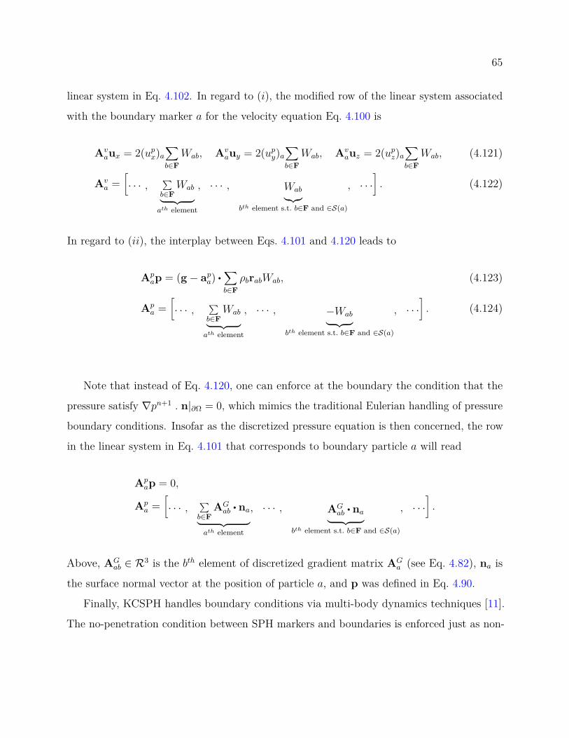
65
linear system in Eq. 4.102. In regard to (i), the modified row of the linear system associated
with the boundary marker a for the velocity equation Eq. 4.100 is
Avaux = 2(upx)a
∑b∈F
Wab, Avauy = 2(upy)a
∑b∈F
Wab, Avauz = 2(upz)a
∑b∈F
Wab, (4.121)
Ava =
[· · · ,
∑b∈F
Wab︸ ︷︷ ︸ath element
, · · · , Wab︸︷︷︸bth element s.t. b∈F and ∈S(a)
, · · ·]. (4.122)
In regard to (ii), the interplay between Eqs. 4.101 and 4.120 leads to
Apap = (g− apa) •
∑b∈F
ρbrabWab, (4.123)
Apa =
[· · · ,
∑b∈F
Wab︸ ︷︷ ︸ath element
, · · · , −Wab︸ ︷︷ ︸bth element s.t. b∈F and ∈S(a)
, · · ·]. (4.124)
Note that instead of Eq. 4.120, one can enforce at the boundary the condition that the
pressure satisfy ∇pn+1 . n|∂Ω = 0, which mimics the traditional Eulerian handling of pressure
boundary conditions. Insofar as the discretized pressure equation is then concerned, the row
in the linear system in Eq. 4.101 that corresponds to boundary particle a will read
Apap = 0,
Apa =
[· · · ,
∑b∈F
AGab• na︸ ︷︷ ︸
ath element
, · · · , AGab• na︸ ︷︷ ︸
bth element s.t. b∈F and ∈S(a)
, · · ·].
Above, AGab ∈ R3 is the bth element of discretized gradient matrix AG
a (see Eq. 4.82), na is
the surface normal vector at the position of particle a, and p was defined in Eq. 4.90.
Finally, KCSPH handles boundary conditions via multi-body dynamics techniques [11].
The no-penetration condition between SPH markers and boundaries is enforced just as non-

66
penetrating contacts are treated in multi-body dynamics; i.e., via unilateral constraints (see
Eq. 3.4). This strategy allows for (i) strict (per marker) enforcement of the no-penetration,
and (ii) more flexibility in terms of the geometry of the boundary. On the downside, this
strategy can only be used to enforce the no-penetration condition but not the no-slip, which
is unlike WCSPH and ISPH.
4.5 Fluid-Solid Interaction
The coupling of the solid and fluid phases is implemented in two stages as shown in Fig. 4.5:
(1) before each time step of the solid phase solver, the forces due to interaction with the fluid
are imposed on each solid object as external forces; and (2) after each time step of the solid
solver, the position and velocity of the solid phase objects are reported to the fluid solver to
provide boundary conditions.
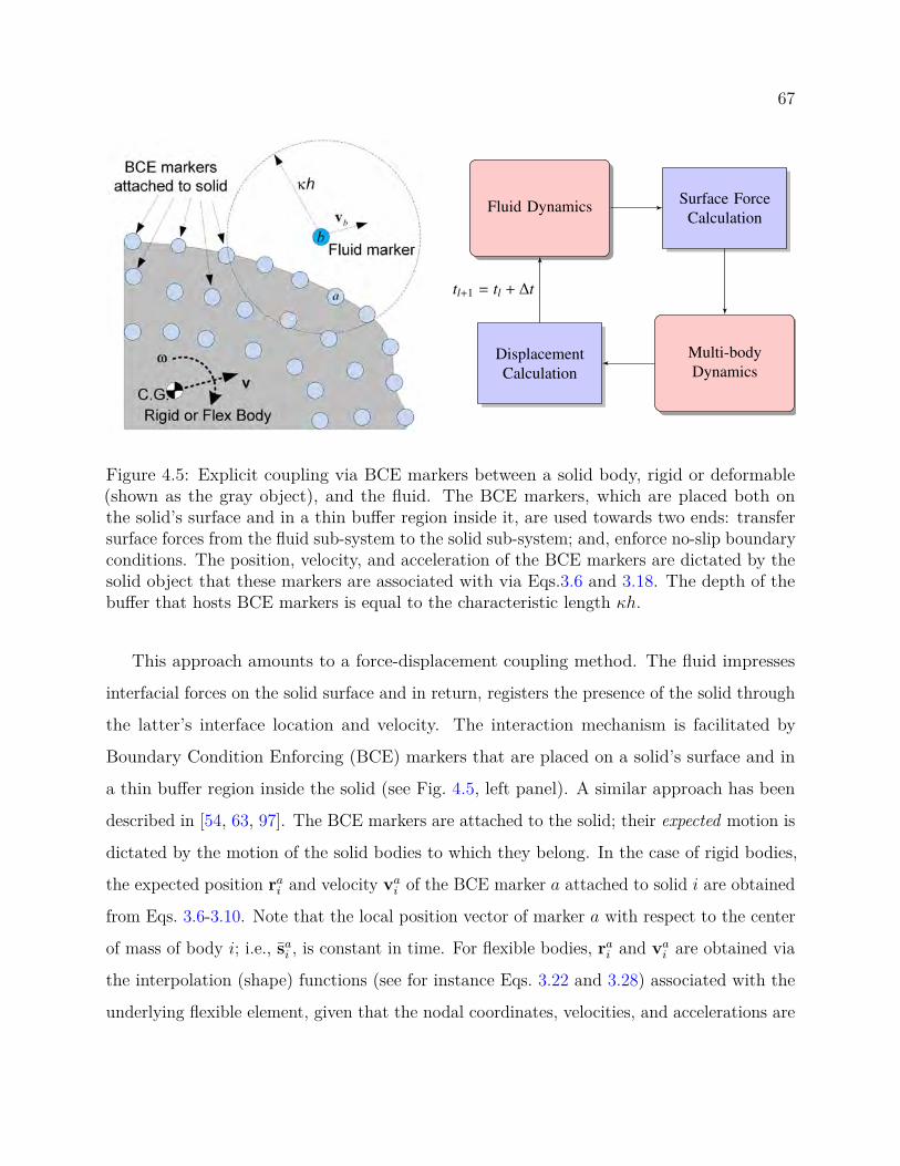
67
Fluid Dynamics Surface ForceCalculation
Multi-bodyDynamics
DisplacementCalculation
tl+1 = tl + ∆t
Figure 4.5: Explicit coupling via BCE markers between a solid body, rigid or deformable(shown as the gray object), and the fluid. The BCE markers, which are placed both onthe solid’s surface and in a thin buffer region inside it, are used towards two ends: transfersurface forces from the fluid sub-system to the solid sub-system; and, enforce no-slip boundaryconditions. The position, velocity, and acceleration of the BCE markers are dictated by thesolid object that these markers are associated with via Eqs.3.6 and 3.18. The depth of thebuffer that hosts BCE markers is equal to the characteristic length κh.
This approach amounts to a force-displacement coupling method. The fluid impresses
interfacial forces on the solid surface and in return, registers the presence of the solid through
the latter’s interface location and velocity. The interaction mechanism is facilitated by
Boundary Condition Enforcing (BCE) markers that are placed on a solid’s surface and in
a thin buffer region inside the solid (see Fig. 4.5, left panel). A similar approach has been
described in [54, 63, 97]. The BCE markers are attached to the solid; their expected motion is
dictated by the motion of the solid bodies to which they belong. In the case of rigid bodies,
the expected position rai and velocity vai of the BCE marker a attached to solid i are obtained
from Eqs. 3.6-3.10. Note that the local position vector of marker a with respect to the center
of mass of body i; i.e., sai , is constant in time. For flexible bodies, rai and vai are obtained via
the interpolation (shape) functions (see for instance Eqs. 3.22 and 3.28) associated with the
underlying flexible element, given that the nodal coordinates, velocities, and accelerations are

68
passed from the solid solver to the fluid solver. For instance, for 1D and 2D elements Eq. 3.23
and Eq. 3.28 can be used, respectively, to obtain the updated position of marker a from the
nodal coordinates qi(t) and similarly to obtain the expected velocity and acceleration from
the nodal velocities qi(t) and accelerations qi(t), respectively. Note that the local natural
coordinates ξ, η, and ζ of the marker attached to the flexible body are constant.
The expected kinematic attributes of the markers, calculated from the motion of the
solid phase at the location occupied by the markers, are different from their assigned values.
The latter are calculated such that the no-slip and no-penetration boundary conditions are
implicitly enforced at the fluid-solid interface. The no-slip condition states that the velocity
of the BCE markers should oppose the velocity of the fluid particles such that the average
relative fluid-solid velocity at the interface is zero; i.e., the average velocity at the interface is
the expected interface velocity. Herein, the induced velocity va at the position of marker a is
computed from the velocity of the fluid markers via Eq. 4.119 as
va =
∑b∈F
vbWab∑b∈F
Wab
.
where F denotes a set of fluid markers that are within the compact support of the BCE marker
a. The no-slip condition holds if (va + va)/2 = vpa; in other words the assigned velocity of
marker a is [96]:
va = 2vpa − va. (4.125)
The pressure of a BCE marker is calculated via a force balance condition at the wall interface,
which leads to Eq. 4.120 as follows [96]
pa =
∑b∈F
pbWab + (g− apa) ·∑b∈F
ρbrabWab∑b∈F
Wab
,
where g is the gravitational acceleration and apa is the acceleration of the solid phase at the
location of marker a. The fluid-solid coupling procedure is described in Algorithm 2.

69
Algorithm 2 Fluid-Solid coupling procedure. Carried out at each time step.1: The fluid phase is integrated in time.2: The pressure and viscous forces exerted by the fluid markers on the BCE markers are
obtained via Eqs. 4.110 and 4.111 for IISPH method, and Eq. 4.103 for WCSPH andISPH methods.
3: The generalized forces on each rigid body or nodal coordinate are calculated by collectingthe forces of their associated BCE markers.
4: Generalized forces are used to solve multibody dynamics involving rigid and flexiblebodies.
5: The position, velocity, and acceleration of the BCE markers are updated based on thenew position, velocity, and acceleration of the rigid and flexible bodies.
6: The velocities and pressure of the BCE markers required for the no-slip and no-penetrationconditions are obtained from Eq. 4.119 and 4.120, respectively.
The fluid-solid coupling strategy outlined in Algorithm 2 will yield slight numerical artifacts
at the interface in relation to incompressibility and/or satisfying no-slip/no-penetration at
the end of a time-step. This is a consequence of the explicit attribute of the coupling strategy.
A fully implicit coupling as provided by a monolithic solver addresses this issue albeit at
an increase in run-time. As a rule of thumb, IISPH, ISPH, and WCSPH yield expeditious
solutions while a monolithic solver such as KCSPH can provide a better quality solution at
the interface yet at a higher computational cost. Certainly, as the time step decreases, ISPH,
IISPH and WCSPH produce increasingly more accurate solutions yet at that point, they
forfeit their inexpensive-solution attribute.
4.6 Viscoplasticity
A robust and accurate numerical implementation of the yield stress in the Navier-Stokes
equations is still a matter of research [1]. The difficulty is in modeling the discontinuity
arising from the yield stress; the material should only flow if the shear stress exceeds the
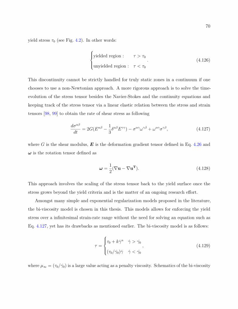
70
yield stress τ0 (see Fig. 4.2). In other words:
yielded region : τ > τ0
unyielded region : τ < τ0
. (4.126)
This discontinuity cannot be strictly handled for truly static zones in a continuum if one
chooses to use a non-Newtonian approach. A more rigorous approach is to solve the time-
evolution of the stress tensor besides the Navier-Stokes and the continuity equations and
keeping track of the stress tensor via a linear elastic relation between the stress and strain
tensors [98, 99] to obtain the rate of shear stress as following
dσαβ
dt= 2G(Eαβ − 1
3δαβEγγ)− σαγωγβ + ωαγσγβ, (4.127)
where G is the shear modulus, E is the deformation gradient tensor defined in Eq. 4.26 and
ω is the rotation tensor defined as
ω = 12(∇u−∇uT). (4.128)
This approach involves the scaling of the stress tensor back to the yield surface once the
stress grows beyond the yield criteria and is the matter of an ongoing research effort.
Amongst many simple and exponential regularization models proposed in the literature,
the bi-viscosity model is chosen in this thesis. This models allows for enforcing the yield
stress over a infinitesimal strain-rate range without the need for solving an equation such as
Eq. 4.127, yet has its drawbacks as mentioned earlier. The bi-viscosity model is as follows:
τ =
τ0 + kγn γ > γ0
(τ0/γ0)γ γ < γ0
, (4.129)
where µ∞ = (τ0/γ0) is a large value acting as a penalty viscosity. Schematics of the bi-viscosity
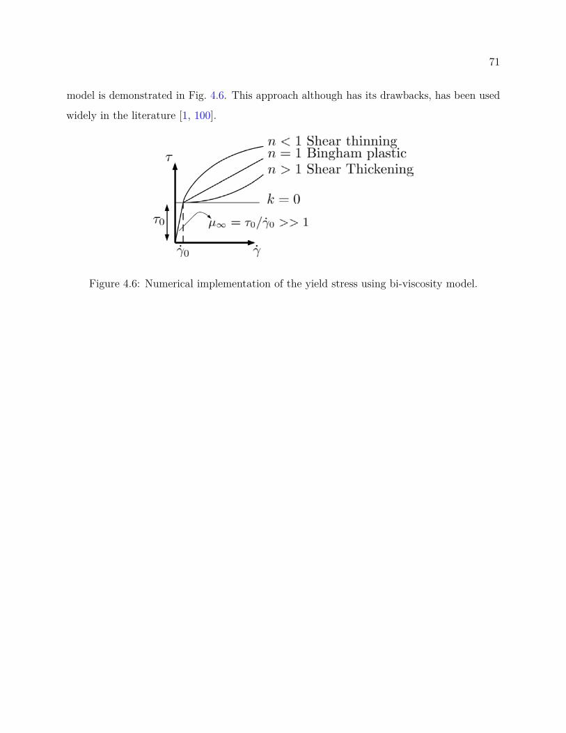
71
model is demonstrated in Fig. 4.6. This approach although has its drawbacks, has been used
widely in the literature [1, 100].
Figure 4.6: Numerical implementation of the yield stress using bi-viscosity model.

72
5 software implementation aspects
This chapter provides details about the software implementation of the multi-physics simu-
lation framework discussed in this thesis along with specifics about the parallel computing
approach. The software implementation is an open-source platform called Chrono, and is
released in public domains under a BSD3 license [101, 102]. Chrono is a cross-platform
(Windows/Linunx/MacOS) middleware and can be embedded in third-party applications. It
is modular and expandable via C++ inheritance and run-time polymorphism.
The high-level overview of the simulation algorithm is as follows. Each subsystem is
responsible for advancing its state to the next simulation time-step. Subsequently, solutions
are coupled at the interface of the continuum and discrete subsystems as shown in Fig. 4.5.
This strategy allows each subsystem to work independently of others within a time-step, and
to choose a suitable parallelization paradigm.
5.1 Overview of Chrono
Chrono is a physics-based parallel-computing modeling and simulation infrastructure based
on a platform-independent and open-source design in C++. Chrono can be employed for
solving a wide range of mechanical systems featuring rigid and flexible body dynamics,
fluid dynamics, and in fluid-solid interaction problems. The core Chrono engine allows for
simulation of mechanisms made of rigid bodies and constraints using a wide set of joints.
It allows for applying motors, linear actuators, springs and dampers as well as forces and
torques. The finite element functionality allows for modeling flexible parts with beams, cables,
shells, solid tetrahedrons and hexahedrons elements and for non-linear analysis with large
deformations. Chrono allows for modeling more involved mechanical systems such as vehicles
using a template-based approach, leveraging a wide set of suspension templates as well as
soil and tire models and powertrains/drivelines. The fluid dynamics module allows for CFD
simulations, and is discussed in the rest of this thesis. The schematic overview of Chrono is
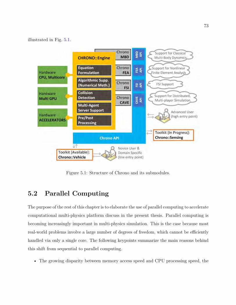
73
illustrated in Fig. 5.1.
Figure 5.1: Structure of Chrono and its submodules.
5.2 Parallel Computing
The purpose of the rest of this chapter is to elaborate the use of parallel computing to accelerate
computational multi-physics platform discuss in the present thesis. Parallel computing is
becoming increasingly important in multi-physics simulation. This is the case because most
real-world problems involve a large number of degrees of freedom, which cannot be efficiently
handled via only a single core. The following keypoints summarize the main reasons behind
this shift from sequential to parallel computing.
• The growing disparity between memory access speed and CPU processing speed, the
74
memory wall, still poses a challenge. This is the case because CPU speeds have increased
regularly, while memory speed, in terms of both the bandwidth and the latency, has
increased at a significantly lower rate.
• Instruction-level parallelism achieved through branch prediction, out-of-order execution
and speculation would require longer horizons and higher power consumption to gain
further improvements.
• Increasing the CPU clock-cycle leads to exponentially-growing energy sinks, which
would require significant improvement in the cooling strategies.
Hence, exploiting parallel computing is necessary to ensure that computer simulation remains
a viable alternative to experimental methods. Herein, the discrete system component of
the solution is the legacy solution implemented in Chrono augmented to support two-way
FSI coupling via BCE markers. It runs on the CPU leveraging multi-core parallelism. The
continuum component of the solution was implemented on the GPU, an architecture suitable
for fine-grained parallelism of the single-instruction-multiple-data type calculation encountered
in SPH discretization. Leveraging hybrid parallel computing by using a multi-core CPU
solution for the discrete phase and a GPU solution for the continuum phase allows to fully
exploit all computational hardware assets available on modern workstations.
5.2.1 CPU Computing Approach
Amongst parallel programming models, the distributed-memory multi-processor architecture,
and shared-memory multi-processor architecture are prime examples that have proven effective
for high-level parallelization.
In the shared-memory multi-processor paradigm, all the processes share the same address
space, i.e., each processor has direct access to the same memory. This model can be leveraged
by APIs such as OpenMP, which offers a low overhead and high-level means to achieve
parallelism. In the OpenMP model, compilers generate parallel execution regions through the

75
use of directives. This idea allows for generating portable and reasonably scalable code, and
running on a wide variety of machines. Most notably, these directives will be safely ignored
on a machine without an OpneMP library and the code will be run sequentially.
In the present work, OpenMP is used for parallelization of computationally intensive parts
of the flexible body dynamics solver. More specifically, computation of the internal loads (see
Eqs. 3.24 and 3.37) and the system Jacobian elements are parallelized via OpenMP parallel
for constructs.
Lastly, Advanced Vector Extension (AVX) intrinsics are used for parallelizing low-level
math operations in this work. The idea of AVX, and other math vectorizing extensions such
as SSE, is to perform a single instruction on multiple pieces of data. This is relevant when
working with low-level matrix operations. For instance, four floats (or two doubles) can be
packed into a single 128 bit register, and one instruction can add the four floats. This idea
makes the underlying matrix operations faster and improves the efficiency of the simulations.
5.2.2 GPU Computing Approach
GPU computing model is based on the concept of a compute accelerator. In this model, a
device separate from the host performs computational tasks and transfer data back to the
host once needed. Graphics Processing Unit (GPU) and Intel’s Xeon Phi are prime examples
of such models.
The hardware of GPUs is different from their CPU counterparts in many ways. One key
architectural difference between CPU and GPU is in the number of physical cores; while a
CPU has fewer of more powerful cores, a GPU has more of less powerful physical cores. GPU
physical cores also run at a lower clock speed. Given this special architecture, GPUs had
been originally designed for video gaming and displaying complex graphics, where rendering
processing hundreds of thousands of polygons in each frame is necessary. Therefore, “single
instruction multiple data” (SIMD) is the parallel paradigm that describes the programming
model suitable for GPU computing.
76
NVIDIA facilitated the use of such devices for computing purposes through the Compute
Unified Device Architecture (CUDA) API and libraries, which assist with building blocks
in computational science. In the present work, the pressure equation is solved via Krylov
subspace methods [103, 104]. For matrix-vector and vector dot product operations, our
Krylov-subspace linear solver relies on two linear algebra libraries provided by NVIDIA:
cuSPARSE [105] and cuBLAS [106].
77
6 validation studies
In this section, verification and validation of various aspects of the numerical method dis-
cussed in Section §3 and §4 are presented. Specifically, the numerical method discussed in
Section §4.4.3 is compared with a finite element counterpart in Section §6.1. Comparison of
numerical methods presented in Sections §4.4.2, §4.4.3, and §4.4.5 is described in Section
§6.2. Verification and validation of the IISPH method (§4.4.4) is described in Section §6.3.
Lastly, the use of regularization (§3.1.4) for obtaining a unique solution for the DVI method
is studied in Section §6.4.
6.1 Lagrangian vs. Eulerian Discretization of
Continua
We report the results of a study in which we compared the Eulerian and Lagrangian approaches
for the solution of free-surface and Fluid-Solid Interaction (FSI) problems. The Eulerian
approach is implemented in another open-source code – Proteus [107], which embraces the
Finite Element Method (FEM). Four tests were considered in this study: flow around a
cylinder, dam break, falling yet floating cylinder in a fluid tank, and an elastic gate problem.
We conclude that the SPH methodology is permissive and expeditious. When compared to
a more robust Eulerian method such as FEM, the SPH solver produces a solution that is
reasonably accurate, computationally less demanding, and easier to produce for the class of
problems investigated in this work. The FEM solver is more accurate as are the methods it
draws on.
6.1.1 The Eulerian Model
In the Eulerian approach, we consider two incompressible Newtonian phases, air and water,
separated by a sharp material interface, across which density and viscosity are discontinuous,

78
but velocity and pressure are continuous. Surface tension is, therefore, neglected.
Denote the domains of the air and water phases as Ωa(t) and Ωw(t). The whole domain is
Ω = Ωw(t) ∪ Ωa(t) and the air/water interface is Γ(t) = ∂Ωw(t) ∩ ∂Ωa(t). The Navier-Stokes
equation above is used to model the motion of each phase of fluid
ρi∂ui
∂t+ ρiui · ∇ui = −∇pi +∇ · τi + fi, x ∈ Ωi(t)
∇ · ui = 0, (6.1)
where ui is the velocity, pi is the pressure, f is the body force, µi is the dynamic viscosity,
σi ≡ −piI + 2µε(ui) is the stress tensor, ε(u) ≡ 12(∇u+∇uT ), and i ∈ w, a.
To solve the Navier-Stokes equations, Eq. 6.1, one has to provide proper boundary
conditions on the exterior boundary ∂Ω and on the interface Γ(t). The boundary condition
on ∂Ω depends on the problem, and, based on the assumption of continuity of velocity and
stress across the interface,
pa = pw, ua = uw, σa · n = σw · n, x ∈ Γ(t) . (6.2)
Using this interface condition (Eq. 6.2) and neglecting the potential loss of smoothness due to
the jump discontinuities in density and viscosity, we can introduce continuous global pressure
and velocity fields p and u and solve a single Navier-Stokes equation
ρ∂u∂t
+ ρu · ∇u = −∇p+∇ · (2µε(u)) + f , x ∈ Ω
∇ · u = 0,
in the whole domain Ω, with ρ := ρw1x∈Ωw(t) + ρa1x∈Ωa(t) and µ := µw1x∈Ωw(t) + µa1x∈Ωa(t).
Note that ρ and µ vary in time and space due the dynamic interface Γ(t). In this work we
use a conservative level set scheme described in [108], which represents the interface Γ(t)
implicitly as the zero level set
φ(t,x) = 0 , (6.3)
79
where φ is the negative of the signed distance to Γ(t) within the water phase and the positive
signed distance in the air phase.
In this approach both an air volume fraction, θ, and the dynamics of the signed distance
field, φ, are modeled based on the governing equations for material surface motion
∂φ
∂t+ u · ∇φ = 0 , (6.4)
and phase volume conservation
∂θ
∂t+∇ · (uθ) = 0 . (6.5)
We then compute ρ and µ as
ρ(t,x) = ρw[1−H(φ)] + ρaH(φ), (6.6)
µ(t,x) = µw[1−H(φ)] + µaH(φ) , (6.7)
where H(·) is the Heaviside step function.
As the solution evolves, the level set φ will gradually lose the signed distance property
and the phase mass conservation property. To simplify the presentation, we assume that
there is no flow through external boundaries, so that for all time the air mass Ma should
maintain the phase mass conservation property
Ma =∫
ΩρaH(φ(t,x) . (6.8)
Note that, under the given assumptions, this statement can be written equivalently as a
volume conservation statement and that analogous statements hold for the water phase.
Several methods have been proposed to correct the violation of these conservation con-
straints, see, for instance [109, 110]. Here we are correcting φ based on the conserved quantity
80
θ as suggested in [108]. The idea is to compute the correction u satisfying the equation
H(φ+ u)− θ = νnum∆u, (6.9)
in order to keep the mass conservation.
As noted above, the use of continuous and differentiable fields for pressure and velocity over
the entire domain Ω is an approximation that is inconsistent with actual jump discontinuities
in density and viscosity. In fact, we use a regularized Heaviside function, Hε(x) as follows
Hε(x) :=
0, if x ≤ −ε
12(1 + x
ε+ 1
φlssin(xφls
ε)) if |x| ≤ ε
1, if x ≥ ε
, (6.10)
to approximate H(x) used in Eqs. 6.6 and 6.7. This represents a first order regularization of
the two-phase flow problem. While much prior work uses this regularization, notable recent
research provides methods and proofs that more precise, second order accurate treatment of
the fluid-fluid interface is achievable in the finite element context [111, 112].
The practice of reinitializing the level set function is a well-established technique in
two-phase flow to control the growth of anomalies and/or numerical errors [113]. In the
present work, we correct the loss of the signed distance property by solving
∂τφ+ sign(φ)(|∇φ| − 1) = 0 , (6.11)
subject to boundary conditions φ = 0 on Γ(t) (i.e., the distance correction does not move the
air-water interface).
The algorithm for the time step tn → tn+1 can be described as follows:
1. Solve Eq. 6.1 with ρ(tn) and µ(tn) defined in Eqs. 6.6 and 6.7 to get the velocity field
un+1 and pressure pn+1
81
2. Solve Eq. 6.4 to get φ∗(tn+1)
3. Solve Eq. 6.5 to get θ∗(tn+1)
4. Solve Eq. 6.11 to get φ∗∗(tn+1) from φ∗(tn+1)
5. Solve 6.9 to get corrected φ(tn+1) and θ = Hε(φ) using φ∗∗(tn+1) and θ∗(tn+1).
We use continuous finite elements to implement an IBM for the solid phase boundary
as well. Let Vh and Mh be the approximation space of the velocity and the pressure. For
the incompressible Navier-Stokes equations, not all pairs Vh ×Mh of piecewise polynomial
spaces are stable, see, for instance [114, 115]. In addition to instabilities that can arise due
to the choice of velocity and pressure spaces, the numerical solution of the Navier-Stokes
equations for Re > 1 can also experience advective instabilities, resulting in velocity (and
pressure) oscillations. In this work we follow the variational multiscale stabilization and shock
capturing method used previously in [108], which introduces additional numerical viscosity in
a manner that stabilizes the advective instabilities as well as the equal-order velocity and
pressure spaces. As these additional terms are unchanged from [108], we will simply reference
them as (stabilization − terms) below. Thus, in addressing point 1 above, the numerical
method used produces un+1 ∈ Vh and pn+1 ∈Mh such that
∫Ωρun+1 − un
τ· v − (ρun+1 · ∇un+1) · v +∇pn+1 · v + 2µε(un+1) : ε(v)− f · v
+∫
Ω[−2µε(un+1)n · v − 2µε(v)n · (un+1 − un+1
S ) + Cαv · (un+1 − un+1S )]δε(d∂ΩS(tn+1)(x))
+∫
ΩCβ(un+1 − un+1
S ) · vHε(d∂ΩS(tn+1)(x))
+∫
Ωun+1 · ∇q
+∫∂ΩD
[−2µε(un+1)n · v − 2µε(v)n · (un+1 − un+1D ) + Cγv · (un+1 − un+1
D )]
+ (stabilization− terms) = 0 ∀v ∈ Vh, q ∈Mh , (6.12)
82
where ε(u) = (∇u+∇u2) and Cα, Cβ, and Cγ are numerical parameters. In this formulation,
the first row is the weak formulation of Navier-Stokes equations with integration-by-parts
applied to the viscous term; the second row is the Nitsche’s method for enforcing the no-slip
boundary condition on the surface of the solid, using the regularized Dirac delta function
δε (derived from Eq. 6.10) to replace the boundary integral with a volume integral; the
third row is the penalty term on the velocity inside the solid; the fourth row is from the
continuity equation; the fifth row is due to the boundary condition of u|∂ΩD(t) = uD(t) and
2νε(u) · n|∂ΩN(t) = g(t) with ∂ΩD ∩ ∂ΩN = ∅ and ∂Ω = ∂ΩD ∪ ∂ΩN .
We solve this system using a first-order operating splitting scheme for variable-coefficient
Navier-Stokes equations following [116]. The first step is to solve for the velocity un+1 by
solving
∫Ωρun+1 − un
τ· v + ρ(u∗ · ∇un+1) · v +∇p# · v + 2µε(un+1) : ε(v)− f · v
+∫
Ω[−2µε(un+1)n · v − 2µε(v)n · (un+1 − un+1
S ) + Cαv · (un+1 − un+1S )]δε(d∂ΩS(tn+1)(x))
+∫
ΩCβ(un+1 − un+1
S ) · vHε(d∂ΩS(tn+1)(x))
+∫∂ΩD
[−2µε(un+1)n · v − 2µε(v)n · (un+1 − un+1D ) + Cγv · (un+1 − un+1
D )]−∫∂ΩN
g · v
+ (stabilization− terms) = 0, ∀v ∈ Vh , (6.13)
where u∗ and p# are the extrapolation of the velocity and the pressure computed as u∗ := un
and p# := pn + φn. This choice results in a linear system for the velocity components. The
2nd step of the projection scheme corrects the velocity field un+1 to obtain a divergence free
velocity field un+1 and an accurate pressure, pn+1. The velocity field un+1 is defined as
un+1 = un+1 − τ
ρmin∇φn+1 ,

83
with the help of the pressure increment, φn+1, which satisfies the Poisson problem
∇ · ∇φn+1 = ∇ · un+1,
with appropriate boundary conditions. For example, at the part of the boundary where un+1
and un+1 are specified, one has to enforce ∇φn+1 · n = 0. The pressure pn+1 is then defined
as
pn+1 := pn + φn+1 − µ∇ · un+1 .
Details pertaining the stability of this algorithm and a proof of second order accuracy in
time when a second order BDF method is used in place of Backward Euler used above are
provided in [116].
In the following, we present and discuss results obtained with the Eulerian and Lagrangian
approaches for four tests. The flow around a cylinder is considered, given that it represents
a widely used single-phase CFD benchmark problem. A dam break test is used to gauge
performance for free-surface flows. Lastly, the two approaches are compared in conjunction
with two FSI problems – one pertaining to a floating rigid body and one that has the fluid
interacting with an elastic/deformable gate.
6.1.2 Flow Around Cylinder
This single-phase, internal flow test is used to compare the FE and SPH solutions for a
benchmark problem where the flow is shaped by the interplay between the pressure gradient,
and the viscous and body forces. The cylinder of radius 0.05m is positioned at the center
of a rectangular domain of height 0.4m and length 1.0m. No-slip boundary conditions are
applied to the top and bottom walls while periodic (cyclic) conditions are maintained at
the left (inlet) and right (outlet) patches. A constant body force fb=1.0m/s2 is applied in
order to balance the viscous force. The density and viscosity are set to ρ0=10.0kg/m3 and

84
µ=0.1Pa s, respectively. As illustrates in Fig 6.1, the steady-state velocity predicted by SPH
and FEM are qualitatively in close agreement.
Figure 6.1: Comparison of the steady-state velocity profiles predicted with SPH (left) andFEM (right). The SPH markers outside the fluid domain are BCE markers, see §4.4.6.
Similarly, the FEM and SPH pressure profiles show close agreement as illustrated in
Fig. 6.2.
Figure 6.2: Comparison of the steady-state pressure profiles predicted with SPH (left) andFEM (right).
Lastly, we quantitatively compare the two methods in terms of drag calculation. Herein,
the expression used for the drag coefficient is Cd = Fd
0.5ρ A U2 , where Fd is the drag force
magnitude along the x axis, ρ = ρ0 and U = 1m/s are the reference density and velocity, and
A is the frontal area of the cylinder. As shown in Fig. 6.3, SPH and FEM show different drag

85
coefficients at the onset of the simulation yet the steady-state solutions are in good agreement–
the relative error of the time-averaged drag coefficient over the last 2s of the simulations is
6.4%. We posit that two reasons contributing to these discrepancies are: (i) the different
time-integration schemes, and (ii) the vastly different space discretization technique and
boundary condition enforcement used in the formulations. The IB method requires a fine mesh
near the solid level-set (cylinder) for accurate representation of the fluid-structure interface
and forces. Handling this interface poses no major challenge to SPH or boundary-fitted
mesh-based approaches, owing to the explicit representation of the fluid-structure interface.
Figure 6.3: Variation of the drag coefficient over time.
6.1.3 Dam Break
This free-surface flow experiment is setup as follows: the fluid domain is a rectangular prism
of size 2m × 1.0m. The reference density and viscosity are ρ = 1000kg/m3 and µ =0.001 Pa s.
The gravity g = −9.8m/s2 is applied in the y direction. The SPH and FEM results are
compared from two perspectives: (i) the fluid front position over time, and (ii) the roll up and
the second splash – two characteristics highlighted in previous studies [117, 96]. As shown in
Fig. 6.4, the SPH solution of the fluid front position over time slightly under-estimate the FEM
solution. SPH has an easier task in handling free-surface since in the Lagrangian framework
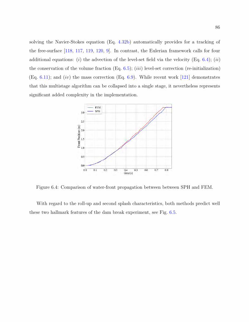
86
solving the Navier-Stokes equation (Eq. 4.32b) automatically provides for a tracking of
the free-surface [118, 117, 119, 120, 9]. In contrast, the Eulerian framework calls for four
additional equations: (i) the advection of the level-set field via the velocity (Eq. 6.4); (ii)
the conservation of the volume fraction (Eq. 6.5); (iii) level-set correction (re-initialization)
(Eq. 6.11); and (iv) the mass correction (Eq. 6.9). While recent work [121] demonstrates
that this multistage algorithm can be collapsed into a single stage, it nevertheless represents
significant added complexity in the implementation.
Figure 6.4: Comparison of water-front propagation between between SPH and FEM.
With regard to the roll-up and second splash characteristics, both methods predict well
these two hallmark features of the dam break experiment, see Fig. 6.5.

87
Figure 6.5: Comparison of the roll-up (t = 1.75s, left) and the second splash (t = 2.05s, right)characteristics between FEM (top) and SPH (bottom)
6.1.4 Fluid Interaction with a Falling Cylinder
This experiment was used to compare the Eulerian and Lagrangian approaches in conjunction
with a 3D scenario that included ample fluid-solid boundary movement. It may be regarded
as a simplified problem that, in more complex forms, is conspicuous in several fluid-structure
interaction applications in coastal and offshore structures, e.g., renewable energy devices and
caissons. Insofar as the solution methodology is concerned, the test assesses the robustness of
the fluid-structure coupling methodology described in §4.5.
The problem is setup as follows. A cylindrical object of radius r = 0.12m and length
L = 0.2m is released from the height h = 0.25m above the surface of a tank of water at
t = 0s. The dimension of the fluid domain is 1.0m × 1.0m × 0.2m (width×height×depth).
The gravity g = −9.8m/s2 is applied in the y direction. The reference density and viscosity
of the water are ρ = 1000kg/m3 and µ =0.001 Pa s. The density of the cylinder is ρs = 0.7ρ,

88
which turns it into a floating structure. Figure 6.6 illustrates the distribution of the pressure
in the frontal cross-section of the domain at t = 0.5s.
The cylinder oscillates until its initial potential energy is damped out. The steady-state
solution of this problem is given by Newton’s second law and basic hydrostatics. Indeed,
the upward buoyant force that is exerted on the body should balance to the weight of the
object; i.e., ρsgV = 62.0. Figure 6.7 illustrates the vertical component of the fluid-structure
interaction forces obtained with FEM and SPH. Although the two models show similar
characteristics and steady-state solution for the vertical force, we note that the SPH model
damps out the oscillation faster due to (i) more numerical damping and, more importantly,
(ii) more degrees of freedom. Specifically, the FEM fluid-structure force uses the smoothed
Heaviside and Dirac delta functions (see Eq. 6.10). This smoothing is numerically done along
he < ε < 2he in the mesh where he is the elements’ characteristic length scale. Incorporating
the information from nodes further away at any point require increasing this smoothing
length, which consequently deteriorates the accuracy of the numerical fluid-structure forces.

89
Figure 6.6: Comparison of the steady-state pressure profiles predicted with SPH (left) andFEM (right).
Figure 6.7: Upward buoyant force exerted to the cylinder over time.
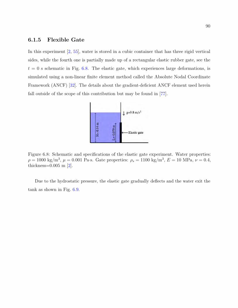
90
6.1.5 Flexible Gate
In this experiment [2, 55], water is stored in a cubic container that has three rigid vertical
sides, while the fourth one is partially made up of a rectangular elastic rubber gate, see the
t = 0 s schematic in Fig. 6.8. The elastic gate, which experiences large deformations, is
simulated using a non-linear finite element method called the Absolute Nodal Coordinate
Framework (ANCF) [32]. The details about the gradient-deficient ANCF element used herein
fall outside of the scope of this contribution but may be found in [77].
Figure 6.8: Schematic and specifications of the elastic gate experiment. Water properties:ρ = 1000 kg/m3, µ = 0.001 Pa·s. Gate properties: ρs = 1100 kg/m3, E = 10 MPa, ν = 0.4,thickness=0.005 m [2].
Due to the hydrostatic pressure, the elastic gate gradually deflects and the water exit the
tank as shown in Fig. 6.9.
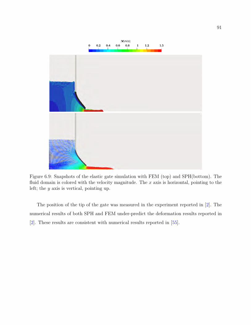
91
Figure 6.9: Snapshots of the elastic gate simulation with FEM (top) and SPH(bottom). Thefluid domain is colored with the velocity magnitude. The x axis is horizontal, pointing to theleft; the y axis is vertical, pointing up.
The position of the tip of the gate was measured in the experiment reported in [2]. The
numerical results of both SPH and FEM under-predict the deformation results reported in
[2]. These results are consistent with numerical results reported in [55].
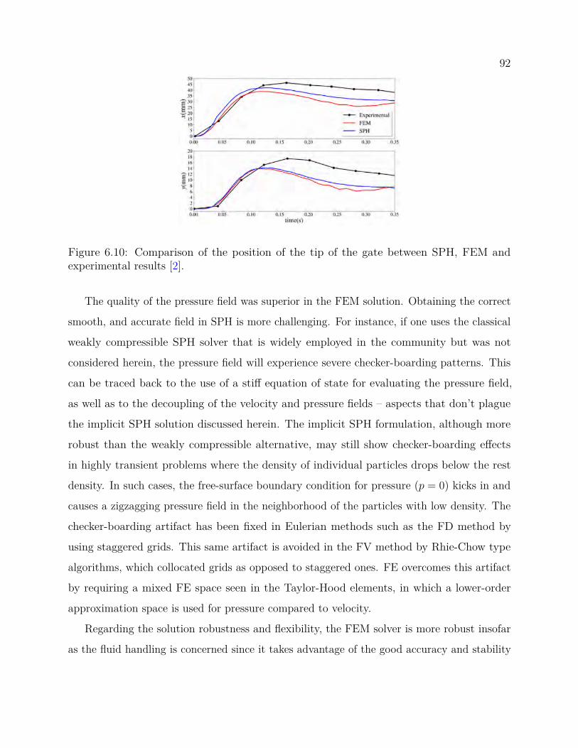
92
Figure 6.10: Comparison of the position of the tip of the gate between SPH, FEM andexperimental results [2].
The quality of the pressure field was superior in the FEM solution. Obtaining the correct
smooth, and accurate field in SPH is more challenging. For instance, if one uses the classical
weakly compressible SPH solver that is widely employed in the community but was not
considered herein, the pressure field will experience severe checker-boarding patterns. This
can be traced back to the use of a stiff equation of state for evaluating the pressure field,
as well as to the decoupling of the velocity and pressure fields – aspects that don’t plague
the implicit SPH solution discussed herein. The implicit SPH formulation, although more
robust than the weakly compressible alternative, may still show checker-boarding effects
in highly transient problems where the density of individual particles drops below the rest
density. In such cases, the free-surface boundary condition for pressure (p = 0) kicks in and
causes a zigzagging pressure field in the neighborhood of the particles with low density. The
checker-boarding artifact has been fixed in Eulerian methods such as the FD method by
using staggered grids. This same artifact is avoided in the FV method by Rhie-Chow type
algorithms, which collocated grids as opposed to staggered ones. FE overcomes this artifact
by requiring a mixed FE space seen in the Taylor-Hood elements, in which a lower-order
approximation space is used for pressure compared to velocity.
Regarding the solution robustness and flexibility, the FEM solver is more robust insofar
as the fluid handling is concerned since it takes advantage of the good accuracy and stability

93
of established Eulerian methods. It also allows for a richer set of boundary condition types
and flow regimes. On the other hand, the SPH solver in our experience is more robust when
dealing with the class of FSI problems studied herein. This is mainly due to its Lagrangian
framework that lends itself well to the coupling between the fluid and solid phases.
6.2 Comparison Between SPH Methods
This section reports on the performance of WCSPH, ISPH and KCSPH in conjunction with
five tests chosen to probe complementary aspects of the CFD solution. Not all solvers are
used for each test; yet each test is run with at least two of the three solvers. A “fluid-at-rest”
test was chosen to gauge effectiveness in enforcing incompressibility; the Poiseuille flow was
selected to verify the accuracy of the viscosity formulation when the pressure forces are
negligible; conversely, the flow around cylinder exposes a scenario in which the pressure
gradient has a significant effect on the flow field; the dam break probes the effectiveness of
each solution for a free-surface problem that displays high transients; and, a liquid sloshing
experiment was selected to assess the ability of WCSPH, ISPH and KCSPH to handle fluid-
solid interaction phenomena. It is noted that by and large, almost all results reported in the
SPH literature are obtained with variations of WCSPH. ISPH has been used in limited cases.
The use of KCSPH has been hardly reported in the literature.
In the following numerical experiments, we use the standard SPH discretizations without
particle shifting for the compressibility test, the dam break, and the sloshing experiments.
We use particle shifting in ISPH and WCSPH for the internal flow experiments such as
the Poiseuille flow and the flow around cylinder experiments in order to maintain regular
particle distribution. Finally, the consistent discretizations are used in ISPH for the Poiseuille
flow and the flow around cylinder experiments to reduce the number of neighbors and the
computational costs of the pressure solver.
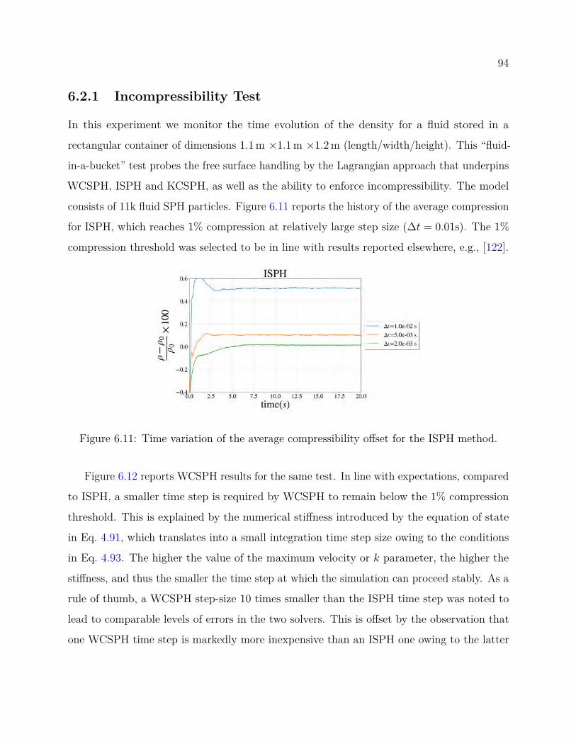
94
6.2.1 Incompressibility Test
In this experiment we monitor the time evolution of the density for a fluid stored in a
rectangular container of dimensions 1.1 m ×1.1 m ×1.2 m (length/width/height). This “fluid-
in-a-bucket” test probes the free surface handling by the Lagrangian approach that underpins
WCSPH, ISPH and KCSPH, as well as the ability to enforce incompressibility. The model
consists of 11k fluid SPH particles. Figure 6.11 reports the history of the average compression
for ISPH, which reaches 1% compression at relatively large step size (∆t = 0.01s). The 1%
compression threshold was selected to be in line with results reported elsewhere, e.g., [122].
Figure 6.11: Time variation of the average compressibility offset for the ISPH method.
Figure 6.12 reports WCSPH results for the same test. In line with expectations, compared
to ISPH, a smaller time step is required by WCSPH to remain below the 1% compression
threshold. This is explained by the numerical stiffness introduced by the equation of state
in Eq. 4.91, which translates into a small integration time step size owing to the conditions
in Eq. 4.93. The higher the value of the maximum velocity or k parameter, the higher the
stiffness, and thus the smaller the time step at which the simulation can proceed stably. As a
rule of thumb, a WCSPH step-size 10 times smaller than the ISPH time step was noted to
lead to comparable levels of errors in the two solvers. This is offset by the observation that
one WCSPH time step is markedly more inexpensive than an ISPH one owing to the latter

95
solver requiring the solution of a Poisson problem.
Figure 6.12: Time variation of the average compressibility offset for the WCSPH method.
Finally, Fig. 6.13 reports KCSPH results. Setting aside the initial transients, KCSPH
enforces incompressibility better than ISPH. This goes back to Eq. 4.114, which imposes
incompressibility in KCSPH assertively. WCSPH lacks this mechanism. Instead, an indirect,
“penalty” approach controls compressibility by a stiff equation of state that penalizes density
drift. One could draw a parallel between WCSPH and a widely used approach to handling
contact forces in granular dynamics, in which one uses a stiff penalty force to enforce non-
penetration conditions (a proxy for volume preservation, or incompressibility) at the mutual
contact point between two elements [34]. Just like in the case of WCSPH, the penalty
approach in contact mechanics requires small integration time steps for numerical stability.
For granular dynamics, a comparison of an assertive (kinematically constrained) approach vs.
a penalty approach is reported in [123].

96
Figure 6.13: Time variation of the average compressibility offset for the KCSPH method.
6.2.2 Poiseuille Flow
An attractive feature of the Poiseuille flow is the availability of a time-dependent analytical
solution. Due to the absence of the pressure gradient term, this test is often used to validate the
accuracy of the viscosity model in the Navier-Stokes equations. This test is run with WCSPH
and ISPH owing to the lack of a viscosity model in the current KCSPH implementation. The
problem is set up as follows: A rectangular domain of fluid with dimensions 1m × 0.2m ×
0.08m (in the direction of flow, width of the channel, depth of the channel) consisting of 24k
SPH particles is subjected to a body force fb = 0.01m/s2 in the positive x direction. Boundary
conditions enforce periodic boundary at the left and right as well as at the front and back
patch pairs of the domain. The top and bottom boundary conditions are no-slip velocity, see
Eq. 4.119. The fluid is accelerated by the body-force and reaches to a steady-state parabolic
velocity profile. The analytical solution of this problem is given by [92]
ux(y, t) = ρ|fb|2µ y(y − L) +
∞∑n=0
4ρ|fb|L2
µπ3(2n+ 1)3 sin(πy
L(2n+ 1)
)exp
(− (2n+ 1)2π2µ
ρL2 t
),
(6.14)

97
Figure 6.14: Velocity profile of transient Poiseuille flow obtained from numerical simulationof WCSPH, ISPH, and series solution at different times.
where ρ0 =1000 kg/m3, µ =1.0 Pa s and L = 0.2 m. The WCSPH and ISPH results show
a close match with the velocity profiles obtained from the analytical solution as shown in
Fig. 6.14. The time required for reaching steady-state solution is assessed according to the
change in the maximum velocity. The relative difference between the maximum velocity
at t = 50s and t = 100s is 0.0001%, making the solution at t = 50s a good approximation
of the steady-state solution for all practical purposes. The average error of the velocity in
the flow direction at t = 50s is 0.1% and 0.7% for ISPH and WCSPH, respectively. The
numerical error associated with the spatial and temporal discretization decrease by increasing
the resolution and decreasing the time step, respectively. The standard discretizations (see
Eqs. (4.62)-(4.63)) are used in the WCSPH formulation along with larger kernel support radius
to maintain the spatial accuracy, while the consistent discretization (see Eqs. (4.65)-(4.66))
is applied in the ISPH formulation. A more in-depth discussion on the accuracy of the
discretization method was presented in [12].
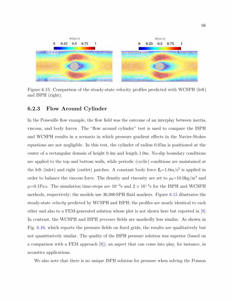
98
Figure 6.15: Comparison of the steady-state velocity profiles predicted with WCSPH (left)and ISPH (right).
6.2.3 Flow Around Cylinder
In the Poiseuille flow example, the flow field was the outcome of an interplay between inertia,
viscous, and body forces. The “flow around cylinder” test is used to compare the ISPH
and WCSPH results in a scenario in which pressure gradient effects in the Navier-Stokes
equations are not negligible. In this test, the cylinder of radius 0.05m is positioned at the
center of a rectangular domain of height 0.4m and length 1.0m. No-slip boundary conditions
are applied to the top and bottom walls, while periodic (cyclic) conditions are maintained at
the left (inlet) and right (outlet) patches. A constant body force fb=1.0m/s2 is applied in
order to balance the viscous force. The density and viscosity are set to ρ0=10.0kg/m3 and
µ=0.1Pa s. The simulation time-steps are 10−3s and 2 × 10⁻⁴s for the ISPH and WCSPH
methods, respectively; the models use 36,000 SPH fluid markers. Figure 6.15 illustrates the
steady-state velocity predicted by WCSPH and ISPH; the profiles are nearly identical to each
other and also to a FEM-generated solution whose plot is not shown here but reported in [8].
In contrast, the WCSPH and ISPH pressure fields are markedly less similar. As shown in
Fig. 6.16, which reports the pressure fields on fixed grids, the results are qualitatively but
not quantitatively similar. The quality of the ISPH pressure solution was superior (based on
a comparison with a FEM approach [8]), an aspect that can come into play, for instance, in
acoustics applications.
We also note that there is no unique ISPH solution for pressure when solving the Poisson

99
Figure 6.16: Comparison of the steady-state pressure profiles predicted with WCSPH (left)and ISPH (right).
equation under pure Neumann boundary conditions – in fact, the pressure solution is unique
up to a constant. In other words, in the absence of Dirichlet boundary conditions, pressure
is a relative quantity in the Navier-Stokes equations. Whereas the reference (minimum)
pressure for WCSPH is often set to zero, in ISPH, we choose the pressure solution with the
average value of zero. Consequently, the difference between the legend of the plots in Fig. 6.16
has no real significance as long as the difference between the solutions is a constant offset
that only indicates a reference pressure. Note that the choice of the reference pressure does
not affect the gradient of the pressure, which is the quantity that comes into play in the
Navier-Stokes equation.
Herein, the expression used for the drag coefficient is Cd = Fd
0.5ρ A U2 , where Fd is the drag
force magnitude along the x axis, ρ = ρ0 and U = 1m/s are the reference density and velocity,
and A is the frontal area of the cylinder. Comparing drag coefficient results is insightful
since this exercise provides a macro-scale perspective that, while looking past micro-scale
fluctuations, captures emergent behavior of practical relevance. As shown in Fig. 6.17, ISPH
and WCSPH show different drag coefficients at the onset of the simulation yet the steady
state solutions are in good agreement – the relative error of the time-averaged drag coefficient
over the last 2s of the simulations is 6.4%. We posit that two reasons contributing to these
discrepancies are: (i) the different time-integration schemes used in the formulations (see
Sections §4.4.3 and §4.4.2), each with its own amount of numerical damping [124]; and (ii)
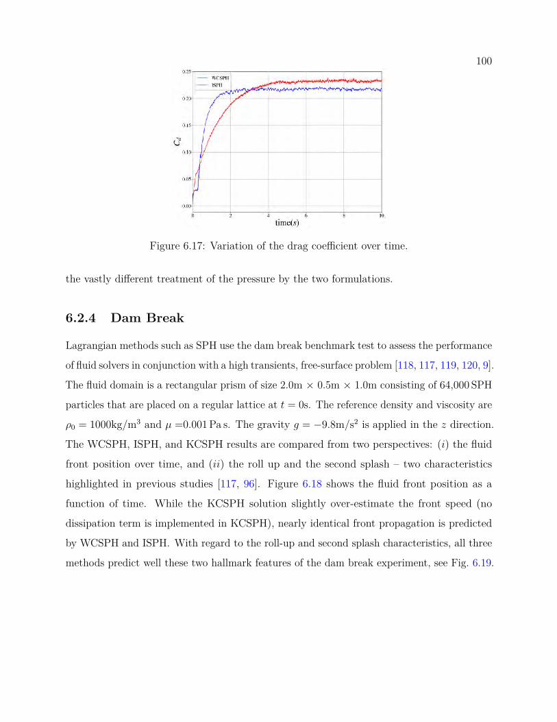
100
Figure 6.17: Variation of the drag coefficient over time.
the vastly different treatment of the pressure by the two formulations.
6.2.4 Dam Break
Lagrangian methods such as SPH use the dam break benchmark test to assess the performance
of fluid solvers in conjunction with a high transients, free-surface problem [118, 117, 119, 120, 9].
The fluid domain is a rectangular prism of size 2.0m × 0.5m × 1.0m consisting of 64,000 SPH
particles that are placed on a regular lattice at t = 0s. The reference density and viscosity are
ρ0 = 1000kg/m3 and µ =0.001 Pa s. The gravity g = −9.8m/s2 is applied in the z direction.
The WCSPH, ISPH, and KCSPH results are compared from two perspectives: (i) the fluid
front position over time, and (ii) the roll up and the second splash – two characteristics
highlighted in previous studies [117, 96]. Figure 6.18 shows the fluid front position as a
function of time. While the KCSPH solution slightly over-estimate the front speed (no
dissipation term is implemented in KCSPH), nearly identical front propagation is predicted
by WCSPH and ISPH. With regard to the roll-up and second splash characteristics, all three
methods predict well these two hallmark features of the dam break experiment, see Fig. 6.19.
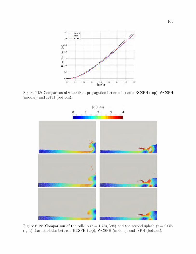
101
Figure 6.18: Comparison of water-front propagation between between KCSPH (top), WCSPH(middle), and ISPH (bottom).
Figure 6.19: Comparison of the roll-up (t = 1.75s, left) and the second splash (t = 2.05s,right) characteristics between KCSPH (top), WCSPH (middle), and ISPH (bottom).

102
6.2.5 Sloshing
Sloshing probes the ability of a CFD solver to handle a free-surface problem that experiences
lower frequency transients (when compared to the dam break). In this experiment a fluid
container undergoes a forced vibration motion according to X0 = sin(2πft), where t is
time, and f and X0 are the frequency and the amplitude of the vibration, respectively. The
analytical solution of this problem under the inviscid flow assumption was discussed in [125]
and involves a set of natural frequencies ωn defined as
ω2n = (2n− 1) π
(g
w
)tanh
[(2n− 1) π
(h
w
)],
where n is the mode number, g is the value of the gravitational acceleration, w is the tank
width; i.e., the tank dimension in the direction of oscillation, and h is the height of the fluid
at rest. The analytical amplitude Fx0 of the net force exerted by the fluid on a sloshing tank
in a forced vibration can then be expressed as
Fx0
Ω2X0ml
= 1 + 8wh
N∑n=1
tanh [(2n− 1) πh/w](2n− 1)3 π3
Ω2
ω2n − Ω2 .
Above, Ω = 2πf is the frequency of the oscillation and ml is the mass of the liquid. The
exerted force on the container in the horizontal direction is expressed as Fx = Fx0sin(2πft).
We compare the ISPH, WCSPH, and KCSPH approximations with the analytical solution
for the following problem: the dimension of the domain (w × b× h) is 1.2m × 0.4m × 1.7m
and the fluid density is ρ0 = 1000kg/m3. The gravity g = −9.8m/s2 is applied in the z
direction. The numerical model is comprised of 98k SPH markers, which are placed on a
uniform Cartesian lattice at t = 0s. The frequency and amplitude of the vibration are set
to be f = 0.75s−1 and X0 = 0.1m. Figure 6.20 reports the sloshing force exerted on the
container over time.
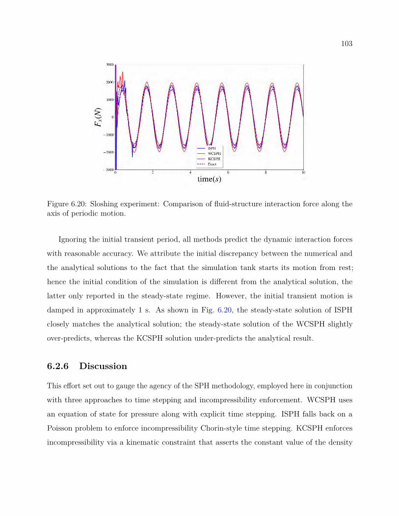
103
Figure 6.20: Sloshing experiment: Comparison of fluid-structure interaction force along theaxis of periodic motion.
Ignoring the initial transient period, all methods predict the dynamic interaction forces
with reasonable accuracy. We attribute the initial discrepancy between the numerical and
the analytical solutions to the fact that the simulation tank starts its motion from rest;
hence the initial condition of the simulation is different from the analytical solution, the
latter only reported in the steady-state regime. However, the initial transient motion is
damped in approximately 1 s. As shown in Fig. 6.20, the steady-state solution of ISPH
closely matches the analytical solution; the steady-state solution of the WCSPH slightly
over-predicts, whereas the KCSPH solution under-predicts the analytical result.
6.2.6 Discussion
This effort set out to gauge the agency of the SPH methodology, employed here in conjunction
with three approaches to time stepping and incompressibility enforcement. WCSPH uses
an equation of state for pressure along with explicit time stepping. ISPH falls back on a
Poisson problem to enforce incompressibility Chorin-style time stepping. KCSPH enforces
incompressibility via a kinematic constraint that asserts the constant value of the density

104
while a half-implicit symplectic Euler integrator is used for time stepping.
WCSPH, ISPH, KCSPH: Ease of implementation comments. WCSPH and ISPH leveraged
GPU computing through CUDA; KCSPH used multi-core parallel computing via OpenMP
[126]. The amount of effort required to implement these solvers in software was quite different.
Implementing the WCSPH solver was easier than ISPH, which was easier than KCSPH.
ISPH requires the solution of a sparse linear system on the GPU; such a solver is not readily
available and herein, the implementation resorted to Krylov subspace iterative methods
such as BICGSTAB and GMRES [127]. A memory-efficient solver requires sparse storage
of the underlying systems (see Eqs. 4.122 and 4.124). Assembling and solving these sparse
linear systems made the ISPH implementation nontrivial. KCSPH was more challenging to
implement since it required at each integration step the solution of a constrained quadratic
optimization problem, see [11]. This optimization problem was posed in hundreds of thousands
of variables – as many as SPH particles used in the formulation and its solution was found
using a Nesterov-type method [128].
WCSPH, ISPH, KCSPH: Solution robustness comments. KCSPH and ISPH provide more
robust (as in less finicky) solutions due to the coupling they establish between the field
variables. Owing to the integration scheme used in ISPH, the velocity and pressure/density
are coupled more tightly than in WCSPH, where pressure depends only on the density.
Similarly in KCSPH, the pressures, which are a proxy of the Lagrange multipliers for the
density kinematic constraints, are coupled with the velocity in a fully implicit sense.
WCSPH, ISPH, KCSPH: Solution quality comments. A simple answer to the question “which
method provides better quality results?” is difficult to provide as multiple factors come into
play in determining the quality of the solution, e.g., the particle resolution, the consistency vs.
conservancy dichotomy, the decision to use or not particle shifting, the size of the time step,
the nature of the problem solved, etc. This question is brought more into focus by stating
that the interest is in obtaining results that are insightful without taxing tinkering with
parameters, settings, etc. In general, ISPH turned out to be easier to set up and get good

105
results with. It is robust (non-finicky) and for a given simulation time budget, it provides
better quality results. One stumbling block is that ISPH requires a sparse linear solver.
WCSPH, particularly for the non-consistent version, usually yields more noisy results – this
also came through in the flow-around-the-cylinder test. KCSPH shows potential, but it needs
further investigation to improve the handling of viscosity and reduce execution speed as it
requires the solution of a constrained convex optimization problem.
WCSPH, ISPH, KCSPH: Time to solution comments. While an efficiency comparison of
WCSPH, ISPH, and KCSPH falls outside the scope of this contribution owing to the sheer
scope of such an undertaking, we considered insightful to provide timing results to understand,
insofar as order of magnitude is concerned, how long an SPH simulation would take. The
problem considered was the dam break simulation of §6.2.4. There was no attempt to optimize
the WCSPH, ISPH, and KCSPH implementations, which were made in Chrono. Therein,
WCSPH and ISPH rely on GPU computing; KCSPH draws on OpenMP. Table 6.2.6 shows
qualitative information regarding the first second of simulation of the dam break problem. All
3D solvers used 215,000 SPH markers. WCSPH takes smaller step sizes due to the explicit
time stepping. However, its effort per time step is both step-size independent and cheaper
than for ISPH or KCSPH. For the latter two, given the iterative nature of the solution
process, higher computational costs are incurred for larger step sizes. Note that even for the
same integration time step, the amount of time required to converge at different points in
the ISPH/KCSPH simulation might be different owing to the difference in the number of
iterations that the underlying linear system/optimization solvers require to converge.
WCSPH, ISPH, KCSPH: Use case recommendations. WCSPH is the method of choice for
many single-phase and free-surface CFD problems such as the dam break and Poiseuille flow.
ISPH was found to be a better choice when more complex physics, e.g., vortex shedding,
boundary layer separation, etc., are present. This is the case for problems like flow around
cylinder and the flow over backward facing step at higher Reynolds numbers (Re ≈ 102–103).
ISPH is also the solver of choice for FSI problems with relatively simple boundary geometries.
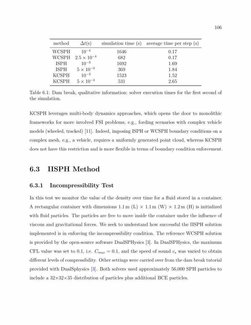
106
method ∆t(s) simulation time (s) average time per step (s)WCSPH 10−4 1646 0.17WCSPH 2.5× 10⁻⁴ 682 0.17
ISPH 10−3 1692 1.69ISPH 5× 10⁻³ 369 1.84
KCSPH 10−3 1523 1.52KCSPH 5× 10⁻³ 531 2.65
Table 6.1: Dam break, qualitative information: solver execution times for the first second ofthe simulation.
KCSPH leverages multi-body dynamics approaches, which opens the door to monolithic
frameworks for more involved FSI problems, e.g., fording scenarios with complex vehicle
models (wheeled, tracked) [11]. Indeed, imposing ISPH or WCSPH boundary conditions on a
complex mesh, e.g., a vehicle, requires a uniformly generated point cloud, whereas KCSPH
does not have this restriction and is more flexible in terms of boundary condition enforcement.
6.3 IISPH Method
6.3.1 Incompressibility Test
In this test we monitor the value of the density over time for a fluid stored in a container.
A rectangular container with dimensions 1.1 m (L) × 1.1 m (W) × 1.2 m (H) is initialized
with fluid particles. The particles are free to move inside the container under the influence of
viscous and gravitational forces. We seek to understand how successful the IISPH solution
implemented is in enforcing the incompressibility condition. The reference WCSPH solution
is provided by the open-source software DualSPHysics [3]. In DualSPHysics, the maximum
CFL value was set to 0.1, i.e. Cmax = 0.1, and the speed of sound cs was varied to obtain
different levels of compressibility. Other settings were carried over from the dam break tutorial
provided with DualSphysics [3]. Both solvers used approximately 56,000 SPH particles to
include a 32×32×35 distribution of particles plus additional BCE particles.

107
Figure 6.21 confirms that increasing cs in WCSPH leads to smaller density errors. However,
the larger cs, the stiffer the numerical problem, which translates into smaller integration
step size. Thus, at one end of the spectrum, WCSPH uses small yet computationally
inexpensive time steps. At the other end of the spectrum, IISPH allows for large albeit more
computationally costly time steps. Against this backdrop, Fig. 6.21 answers the following
question: what value of cs and ∆tWCSPH should be used for DualSPHysics so that the quality
of the solutions produced by IISPH and WCSPH are comparable? As shown in Fig. 6.21, an
approximately 100-fold larger time step can be adopted by the IISPH method for the same
level of compression. The vertical axis in the figure shows the relative error at every time
step, which is defined, for the time step (l) as
% error(l) ≡ ( 1ρ0NF
NF∑i=1
ρ(l)i − 1)× 100 ,
where NF is the number of SPH particles; in Fig. 6.21, “tol” stands for the tolerance used in
the linear solver. Recall though that the larger IISPH step size comes at the cost of solving a
linear system of equations at each time step.

108
Figure 6.21: IISPH vs. WCSPH (DualSPHysics [3]) comparison based on the relative drift inthe incompressibility.
6.3.2 Flow Around a Cylinder
The IISPH results have been compared with results of a finite volume method simulation run
in OpenFOAM [129]. In this test, a cylinder of radius 0.05 m was positioned at the center of
a rectangular domain of height 0.4 m and length 1.0 m. No-slip boundary conditions were
applied to the top and bottom walls while periodic (cyclic) conditions were maintained at the
left (inlet) and right (outlet) patches. A constant body force of fb=0.02 m/s2 was applied in
order to balance the viscous forces. The study was conducted at Re = ρVmaxD/µ ≈ 30.
In order to model the problem in OpenFOAM, a block-structured mesh was created in
blockMesh. In the neighborhood of the cylinder, the size of the mesh-element was chosen
equal to the SPH characteristic length h (see Eq. 4.61). The OpenFOAM pimpleFoam
solver was employed to reach the steady state solution and fvOptions was used to apply
a body force (source term) to the momentum equations. The simulation was run for 10 s
to reach steady state. A dynamic time-step was adopted to maintain Vmax∆t/∆x = 0.2.
Other settings were kept similar to the configuration of the elipsekkLOmega OpenFOAM
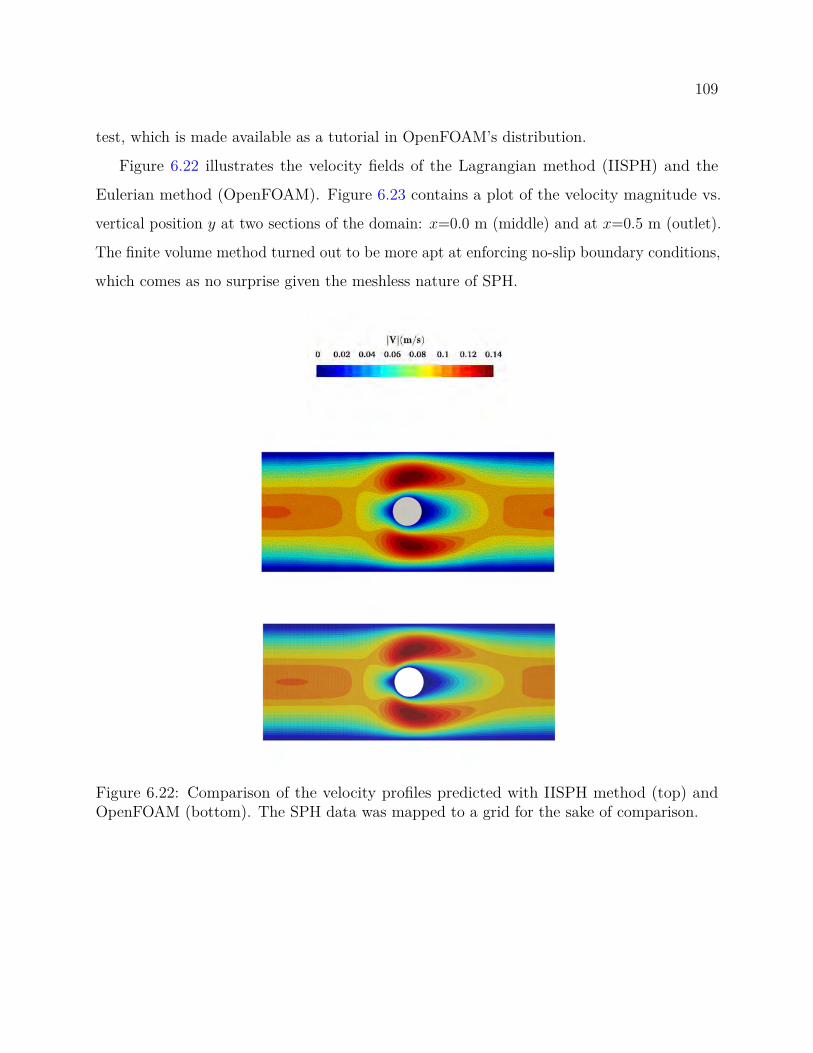
109
test, which is made available as a tutorial in OpenFOAM’s distribution.
Figure 6.22 illustrates the velocity fields of the Lagrangian method (IISPH) and the
Eulerian method (OpenFOAM). Figure 6.23 contains a plot of the velocity magnitude vs.
vertical position y at two sections of the domain: x=0.0 m (middle) and at x=0.5 m (outlet).
The finite volume method turned out to be more apt at enforcing no-slip boundary conditions,
which comes as no surprise given the meshless nature of SPH.
Figure 6.22: Comparison of the velocity profiles predicted with IISPH method (top) andOpenFOAM (bottom). The SPH data was mapped to a grid for the sake of comparison.
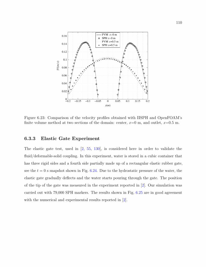
110
Figure 6.23: Comparison of the velocity profiles obtained with IISPH and OpenFOAM’sfinite volume method at two sections of the domain: center, x=0 m, and outlet, x=0.5 m.
6.3.3 Elastic Gate Experiment
The elastic gate test, used in [2, 55, 130], is considered here in order to validate the
fluid/deformable-solid coupling. In this experiment, water is stored in a cubic container that
has three rigid sides and a fourth side partially made up of a rectangular elastic rubber gate,
see the t = 0 s snapshot shown in Fig. 6.24. Due to the hydrostatic pressure of the water, the
elastic gate gradually deflects and the water starts pouring through the gate. The position
of the tip of the gate was measured in the experiment reported in [2]. Our simulation was
carried out with 79,000 SPH markers. The results shown in Fig. 6.25 are in good agreement
with the numerical and experimental results reported in [2].

111
Figure 6.24: Schematic and specifications of the elastic gate experiment. Water properties:ρ = 1000 kg/m3, µ = 0.001 Pa·s. Gate properties: ρs = 1100 kg/m3, E = 10 MPa, ν = 0.4,thickness=0.005 m [2].
0.05 0.1 0.15 0.2 0.25 0.3 0.350.51.01.52.02.53.03.54.04.55.05.5·10−2
t(s)
x(m)
Present StudyAntoci et al. [2]Experimental Results [2]
0.05 0.1 0.15 0.2 0.25 0.3 0.35 0.40.20.40.60.81.01.21.41.61.82.0 ·10−2
t(s)
y(m)
Figure 6.25: Comparison of the horizontal position of the tip of the elastic gate from thenumerical results of the present study, and the numerical/experimental results of the studyof Antoci et al. [2].
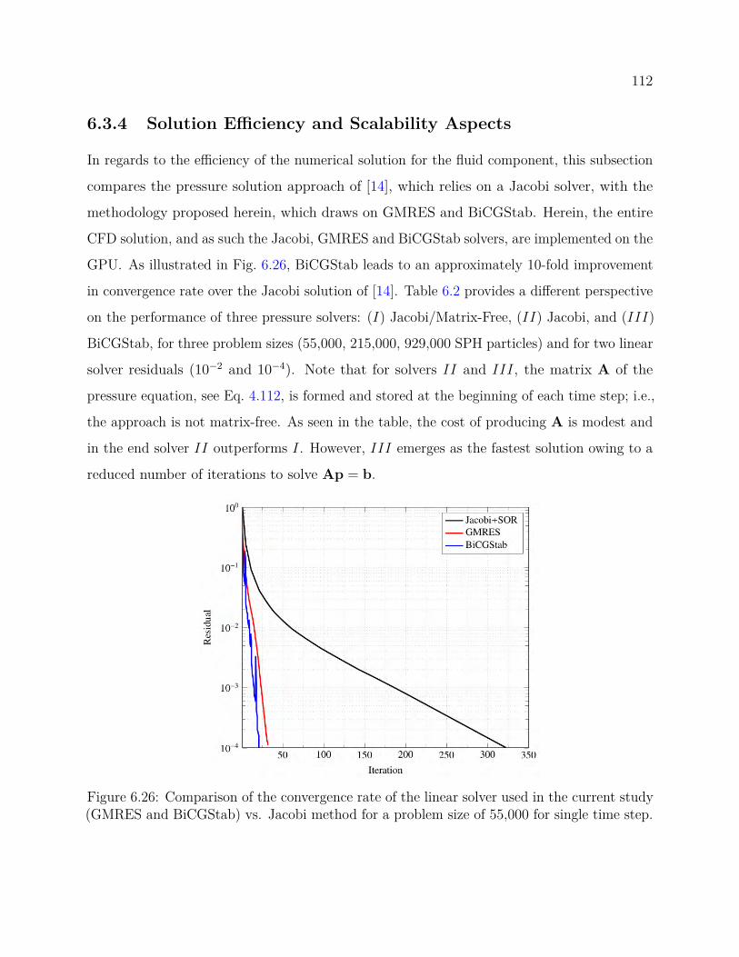
112
6.3.4 Solution Efficiency and Scalability Aspects
In regards to the efficiency of the numerical solution for the fluid component, this subsection
compares the pressure solution approach of [14], which relies on a Jacobi solver, with the
methodology proposed herein, which draws on GMRES and BiCGStab. Herein, the entire
CFD solution, and as such the Jacobi, GMRES and BiCGStab solvers, are implemented on the
GPU. As illustrated in Fig. 6.26, BiCGStab leads to an approximately 10-fold improvement
in convergence rate over the Jacobi solution of [14]. Table 6.2 provides a different perspective
on the performance of three pressure solvers: (I) Jacobi/Matrix-Free, (II) Jacobi, and (III)
BiCGStab, for three problem sizes (55,000, 215,000, 929,000 SPH particles) and for two linear
solver residuals (10−2 and 10−4). Note that for solvers II and III, the matrix A of the
pressure equation, see Eq. 4.112, is formed and stored at the beginning of each time step; i.e.,
the approach is not matrix-free. As seen in the table, the cost of producing A is modest and
in the end solver II outperforms I. However, III emerges as the fastest solution owing to a
reduced number of iterations to solve Ap = b.
Figure 6.26: Comparison of the convergence rate of the linear solver used in the current study(GMRES and BiCGStab) vs. Jacobi method for a problem size of 55,000 for single time step.
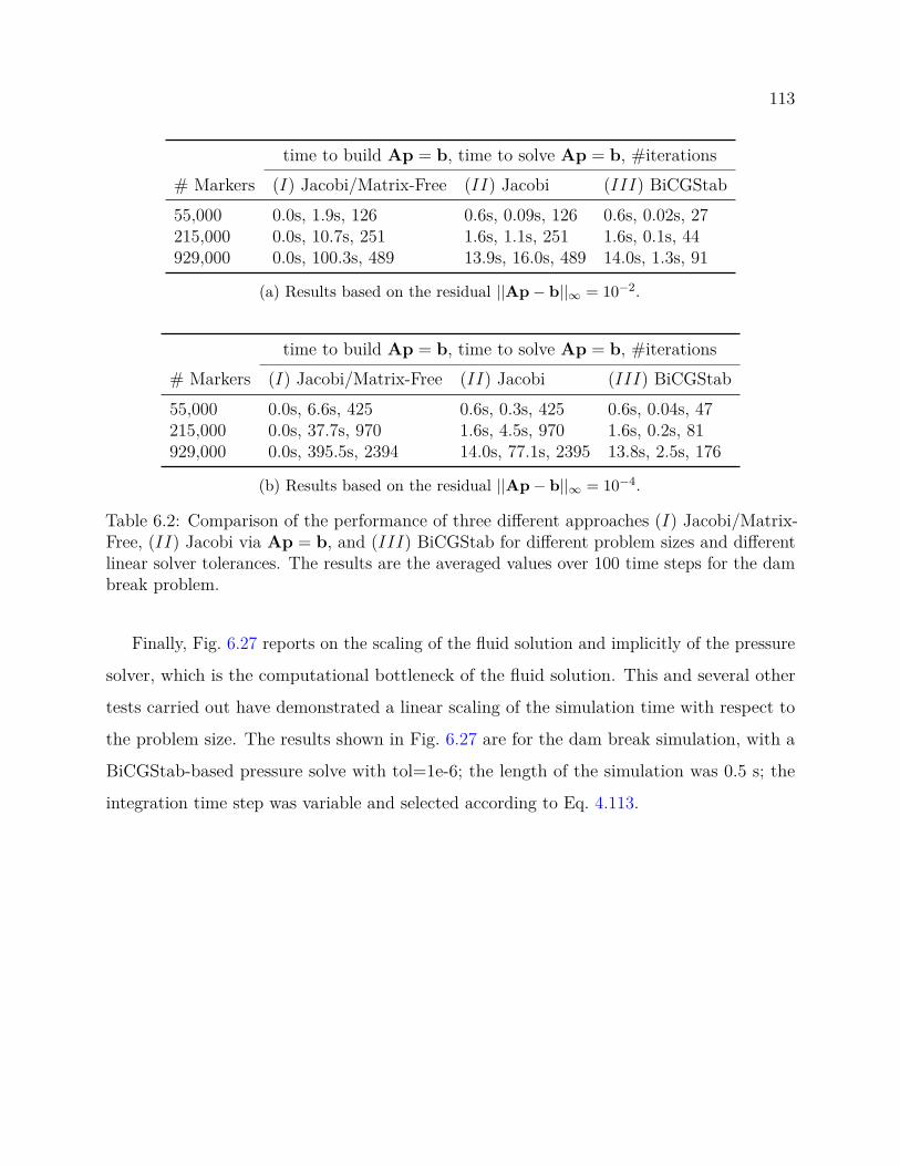
113
time to build Ap = b, time to solve Ap = b, #iterations# Markers (I) Jacobi/Matrix-Free (II) Jacobi (III) BiCGStab55,000 0.0s, 1.9s, 126 0.6s, 0.09s, 126 0.6s, 0.02s, 27215,000 0.0s, 10.7s, 251 1.6s, 1.1s, 251 1.6s, 0.1s, 44929,000 0.0s, 100.3s, 489 13.9s, 16.0s, 489 14.0s, 1.3s, 91
(a) Results based on the residual ||Ap− b||∞ = 10−2.
time to build Ap = b, time to solve Ap = b, #iterations# Markers (I) Jacobi/Matrix-Free (II) Jacobi (III) BiCGStab55,000 0.0s, 6.6s, 425 0.6s, 0.3s, 425 0.6s, 0.04s, 47215,000 0.0s, 37.7s, 970 1.6s, 4.5s, 970 1.6s, 0.2s, 81929,000 0.0s, 395.5s, 2394 14.0s, 77.1s, 2395 13.8s, 2.5s, 176
(b) Results based on the residual ||Ap− b||∞ = 10−4.
Table 6.2: Comparison of the performance of three different approaches (I) Jacobi/Matrix-Free, (II) Jacobi via Ap = b, and (III) BiCGStab for different problem sizes and differentlinear solver tolerances. The results are the averaged values over 100 time steps for the dambreak problem.
Finally, Fig. 6.27 reports on the scaling of the fluid solution and implicitly of the pressure
solver, which is the computational bottleneck of the fluid solution. This and several other
tests carried out have demonstrated a linear scaling of the simulation time with respect to
the problem size. The results shown in Fig. 6.27 are for the dam break simulation, with a
BiCGStab-based pressure solve with tol=1e-6; the length of the simulation was 0.5 s; the
integration time step was variable and selected according to Eq. 4.113.
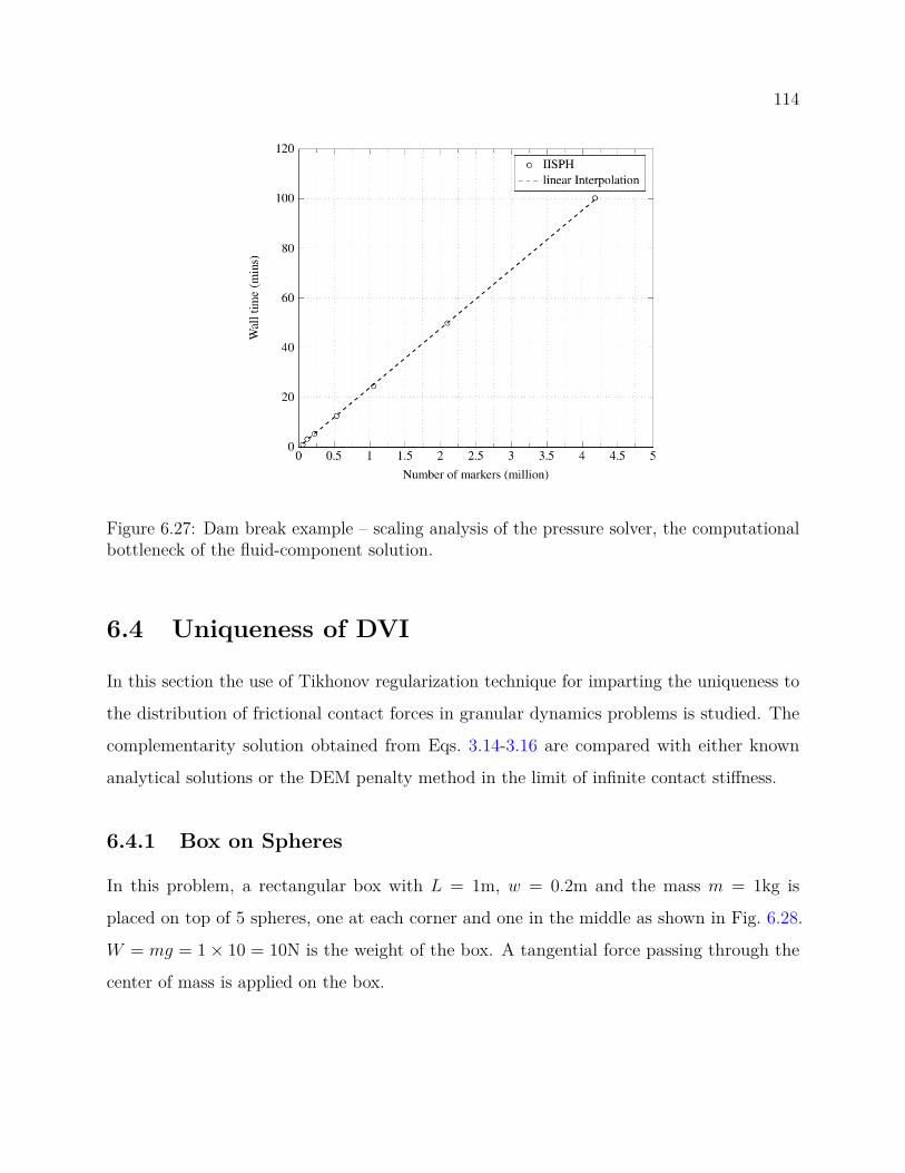
114
Figure 6.27: Dam break example – scaling analysis of the pressure solver, the computationalbottleneck of the fluid-component solution.
6.4 Uniqueness of DVI
In this section the use of Tikhonov regularization technique for imparting the uniqueness to
the distribution of frictional contact forces in granular dynamics problems is studied. The
complementarity solution obtained from Eqs. 3.14-3.16 are compared with either known
analytical solutions or the DEM penalty method in the limit of infinite contact stiffness.
6.4.1 Box on Spheres
In this problem, a rectangular box with L = 1m, w = 0.2m and the mass m = 1kg is
placed on top of 5 spheres, one at each corner and one in the middle as shown in Fig. 6.28.
W = mg = 1× 10 = 10N is the weight of the box. A tangential force passing through the
center of mass is applied on the box.
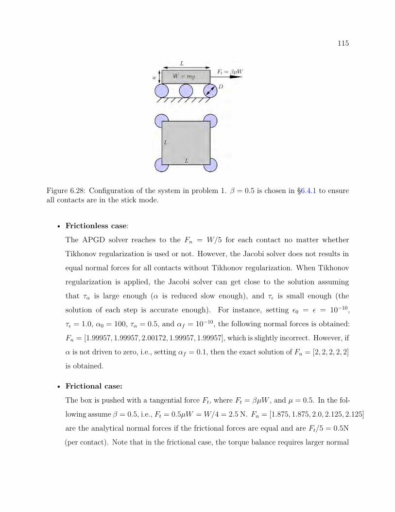
115
Figure 6.28: Configuration of the system in problem 1. β = 0.5 is chosen in §6.4.1 to ensureall contacts are in the stick mode.
• Frictionless case:
The APGD solver reaches to the Fn = W/5 for each contact no matter whether
Tikhonov regularization is used or not. However, the Jacobi solver does not results in
equal normal forces for all contacts without Tikhonov regularization. When Tikhonov
regularization is applied, the Jacobi solver can get close to the solution assuming
that τα is large enough (α is reduced slow enough), and τε is small enough (the
solution of each step is accurate enough). For instance, setting ε0 = ε = 10−10,
τε = 1.0, α0 = 100, τα = 0.5, and αf = 10−10, the following normal forces is obtained:
Fn = [1.99957, 1.99957, 2.00172, 1.99957, 1.99957], which is slightly incorrect. However, if
α is not driven to zero, i.e., setting αf = 0.1, then the exact solution of Fn = [2, 2, 2, 2, 2]
is obtained.
• Frictional case:
The box is pushed with a tangential force Ft, where Ft = βµW , and µ = 0.5. In the fol-
lowing assume β = 0.5, i.e., Ft = 0.5µW = W/4 = 2.5 N. Fn = [1.875, 1.875, 2.0, 2.125, 2.125]
are the analytical normal forces if the frictional forces are equal and are Ft/5 = 0.5N
(per contact). Note that in the frictional case, the torque balance requires larger normal
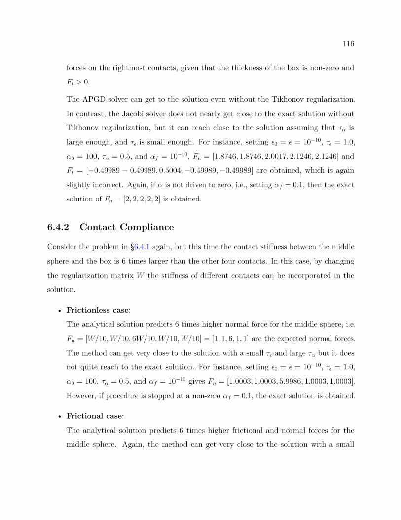
116
forces on the rightmost contacts, given that the thickness of the box is non-zero and
Ft > 0.
The APGD solver can get to the solution even without the Tikhonov regularization.
In contrast, the Jacobi solver does not nearly get close to the exact solution without
Tikhonov regularization, but it can reach close to the solution assuming that τα is
large enough, and τε is small enough. For instance, setting ε0 = ε = 10−10, τε = 1.0,
α0 = 100, τα = 0.5, and αf = 10−10, Fn = [1.8746, 1.8746, 2.0017, 2.1246, 2.1246] and
Ft = [−0.49989 − 0.49989, 0.5004,−0.49989,−0.49989] are obtained, which is again
slightly incorrect. Again, if α is not driven to zero, i.e., setting αf = 0.1, then the exact
solution of Fn = [2, 2, 2, 2, 2] is obtained.
6.4.2 Contact Compliance
Consider the problem in §6.4.1 again, but this time the contact stiffness between the middle
sphere and the box is 6 times larger than the other four contacts. In this case, by changing
the regularization matrix W the stiffness of different contacts can be incorporated in the
solution.
• Frictionless case:
The analytical solution predicts 6 times higher normal force for the middle sphere, i.e.
Fn = [W/10,W/10, 6W/10,W/10,W/10] = [1, 1, 6, 1, 1] are the expected normal forces.
The method can get very close to the solution with a small τε and large τα but it does
not quite reach to the exact solution. For instance, setting ε0 = ε = 10−10, τε = 1.0,
α0 = 100, τα = 0.5, and αf = 10−10 gives Fn = [1.0003, 1.0003, 5.9986, 1.0003, 1.0003].
However, if procedure is stopped at a non-zero αf = 0.1, the exact solution is obtained.
• Frictional case:
The analytical solution predicts 6 times higher frictional and normal forces for the
middle sphere. Again, the method can get very close to the solution with a small

117
τε and large τα. For instance, setting ε0 = ε = 10−10, τε = 1.0, α0 = 100, τα =
0.5, and αf = 10−10 gives Fn = [0.8754, 0.8754, 5.9982, 1.1254, 1.1254] and Ft =
[−0.2501,−0.2501,−1.4995,−0.2501,−0.2501]. Similar to previous scenarios, a nonzero
αf = 0.1 results in fewer total iterations and higher accuracy.
6.4.3 Random Initialization
Consider problem 1, where the initial starting point of the optimization problem is chosen
randomly at every step. Under these conditions, even the APGD solver fails to converge to
the analytical solution discussed above (for both frictional and frictionless case), but with
the Tikhonov regularization the solver converges to the actual solution. In the following, we
study the behavior of the APGD solver with a random initial starting point for slip and stick
mode. At the beginning of the simulation, the box is released from a small distance above
the spheres. The initial stage of the simulations shown in Figs. 6.29 and 6.31 illustrate this
transition. After t = 2.5s the tangential force shown in Fig. 6.28 is applied.
• Stick:
In the following, we assume that β = 0.5, and µ = 0.5, i.e., Ft = 2.5N. In this
configuration, all contacts are in the stick-mode. As shown in Fig. 6.29, the solution
with minimum norm cannot be reached when no regularization is applied, while the
minimum norm solution that predicts similar tangential contact forces is reached with
regularization. Note that the tangential contact forces are all 0.5N although normal
contact forces differ. This is because the friction forces experienced by all contacts i
are still less than the maximum static friction, i.e., 0.5 < µF iNN.
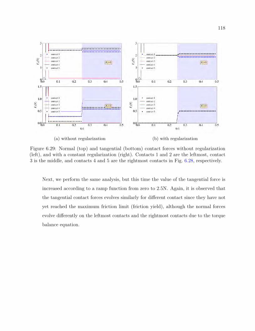
118
(a) without regularization (b) with regularization
Figure 6.29: Normal (top) and tangential (bottom) contact forces without regularization(left), and with a constant regularization (right). Contacts 1 and 2 are the leftmost, contact3 is the middle, and contacts 4 and 5 are the rightmost contacts in Fig. 6.28, respectively.
Next, we perform the same analysis, but this time the value of the tangential force is
increased according to a ramp function from zero to 2.5N. Again, it is observed that
the tangential contact forces evolves similarly for different contact since they have not
yet reached the maximum friction limit (friction yield), although the normal forces
evolve differently on the leftmost contacts and the rightmost contacts due to the torque
balance equation.

119
(a) without regularization (b) with regularization
Figure 6.30: The tangential force is increased from 0 to 2.5N instead of a ramp function,while other parameters remain similar to the ones in Fig. 6.29
• Slip:
In the following, we assume that β = 1.5, and µ = 0.5, i.e., Ft = 7.5N. Given that
Ft = βµN > µN , all contacts are in slip mode. As shown in Fig. 6.31, the solution
with minimum norm cannot be reached when no regularization is applied, while the
minimum norm solution can be obtained when regularization is applied. Note that each
tangential contact forces are linearly dependent on the corresponding normal force. This
is because the friction forces experienced by all contacts i are equal to the maximum
friction, i.e., F it = µF i
N . Also note that the rightmost contact forces increase by time,
while the leftmost contact forces decrease. This has to do with the force balance around
the center of mass of the box, and the position of the contacts with respect to the box,
which changes due to the slip.

120
(a) without regularization (b) with regularization
Figure 6.31: Normal (top) and tangential (bottom) contact forces without regularization(left), and with a constant regularization (right). Contacts 1 and 2 are the leftmost, contact3 is the middle, and contacts 4 and 5 are the rightmost contacts in Fig. 6.28, respectively.
Next, the similar analysis is performed with the tangential force following a ramp
function instead of a step function.
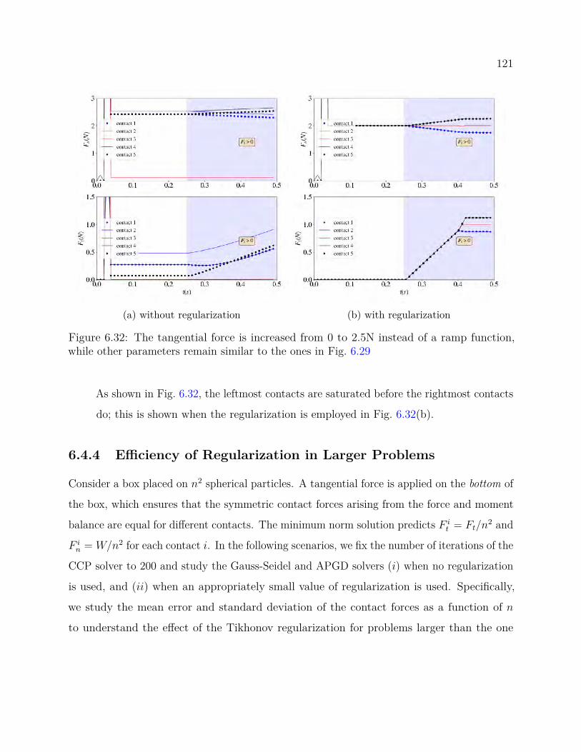
121
(a) without regularization (b) with regularization
Figure 6.32: The tangential force is increased from 0 to 2.5N instead of a ramp function,while other parameters remain similar to the ones in Fig. 6.29
As shown in Fig. 6.32, the leftmost contacts are saturated before the rightmost contacts
do; this is shown when the regularization is employed in Fig. 6.32(b).
6.4.4 Efficiency of Regularization in Larger Problems
Consider a box placed on n2 spherical particles. A tangential force is applied on the bottom of
the box, which ensures that the symmetric contact forces arising from the force and moment
balance are equal for different contacts. The minimum norm solution predicts F it = Ft/n
2 and
F in = W/n2 for each contact i. In the following scenarios, we fix the number of iterations of the
CCP solver to 200 and study the Gauss-Seidel and APGD solvers (i) when no regularization
is used, and (ii) when an appropriately small value of regularization is used. Specifically,
we study the mean error and standard deviation of the contact forces as a function of n
to understand the effect of the Tikhonov regularization for problems larger than the one

122
discussed in problem 1. Mean error and standard deviation of the contact forces are chosen
as measures of solution accuracy and indeterminacy, respectively.
Figure 6.33: A square box with the mass m = 1kg is placed on n2 spherical particles eachwith diameter D.
• Gauss-Seidel solver:
This solver is known for breaking the symmetry owing to its algorithmic asymmetry
[131]. Given the fixed number of iterations mentioned above, it is observed that applying
the regularization to the solver makes possible (i) reaching a more accurate solution
(see mean error) for a fixed number of iterations, and (ii) reducing the indeterminacy
of the system.
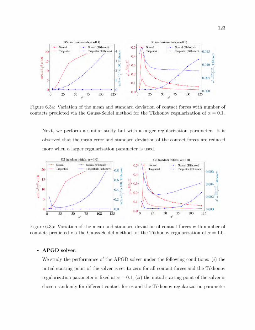
123
Figure 6.34: Variation of the mean and standard deviation of contact forces with number ofcontacts predicted via the Gauss-Seidel method for the Tikhonov regularization of α = 0.1.
Next, we perform a similar study but with a larger regularization parameter. It is
observed that the mean error and standard deviation of the contact forces are reduced
more when a larger regularization parameter is used.
Figure 6.35: Variation of the mean and standard deviation of contact forces with number ofcontacts predicted via the Gauss-Seidel method for the Tikhonov regularization of α = 1.0.
• APGD solver:
We study the performance of the APGD solver under the following conditions: (i) the
initial starting point of the solver is set to zero for all contact forces and the Tikhonov
regularization parameter is fixed at α = 0.1, (ii) the initial starting point of the solver is
chosen randomly for different contact forces and the Tikhonov regularization parameter
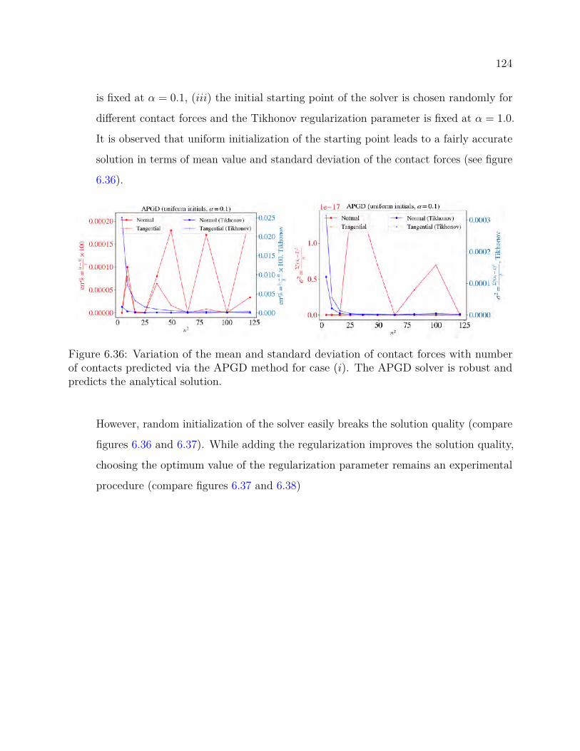
124
is fixed at α = 0.1, (iii) the initial starting point of the solver is chosen randomly for
different contact forces and the Tikhonov regularization parameter is fixed at α = 1.0.
It is observed that uniform initialization of the starting point leads to a fairly accurate
solution in terms of mean value and standard deviation of the contact forces (see figure
6.36).
Figure 6.36: Variation of the mean and standard deviation of contact forces with numberof contacts predicted via the APGD method for case (i). The APGD solver is robust andpredicts the analytical solution.
However, random initialization of the solver easily breaks the solution quality (compare
figures 6.36 and 6.37). While adding the regularization improves the solution quality,
choosing the optimum value of the regularization parameter remains an experimental
procedure (compare figures 6.37 and 6.38)

125
Figure 6.37: Variation of the mean and standard deviation of contact forces with numberof contacts predicted via the APGD method for case (ii). The APGD solver is unable toreach to an accurate solution while a small regularization parameter can slightly improve thesolution quality.
Figure 6.38: Variation of the mean and standard deviation of contact forces with number ofcontacts predicted via the APGD method for case (iii). Similar to case (ii) the APGD solveris unable to reach to an accurate solution but using larger regularization parameter one canrestore the solution quality.
6.4.5 Cannonball Packing
In this problem, we study a square-based pyramid of close-packed spheres, as shown in
Fig. 6.39. N2 spheres are placed at the bottom, and the bottom layer spheres are fixed. The
gravity −10 m/s2 is applied in the vertical direction. In all the cases, we compare the DVI

126
solution with the DEM solution. The DEM parameters are as follows: E = 10Pa is the Young
modulus, ∆t = 2× 10⁻⁵s is the time-step chosen for the DEM solver. Note that herein we
retain the stabilization term 1∆t2 Φ in the the original p = 1
∆t2 Φ + 1∆tBv + BM−1Fext term.
Figure 6.39: Configuration of the cannonball packing. Spheres have radius of 0.1m and massof 1kg. The initial spacing between the spheres is 2% of the radius.
• Frictionless case with N = 6:
First, we investigate the solution of the Tikhonov-modified problem, for the frictionless
case. As illustrated in Fig. 6.40, the tangential contact forces are zero, while there are
slight differences between the normal forces predicted by DVI and DEM. Adding the
Tikhonov regularization term (see Eq. 3.16) does not have a significant effect on the
quality of the solution in this case.
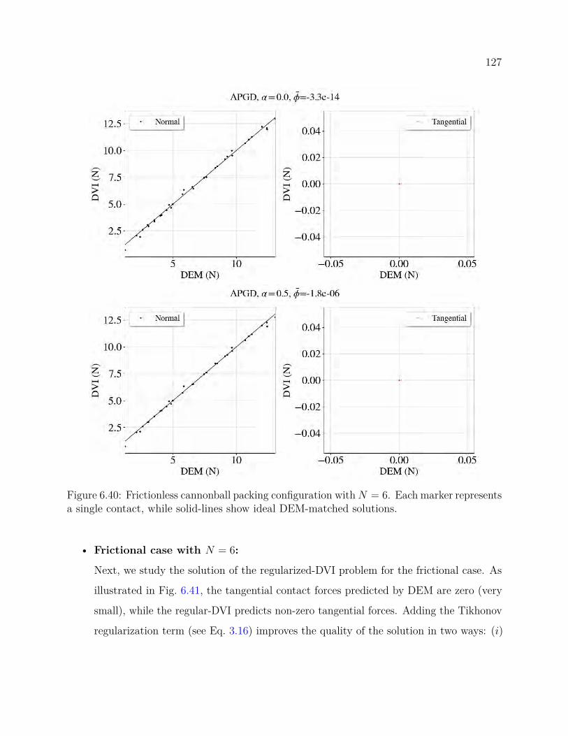
127
Figure 6.40: Frictionless cannonball packing configuration withN = 6. Each marker representsa single contact, while solid-lines show ideal DEM-matched solutions.
• Frictional case with N = 6:
Next, we study the solution of the regularized-DVI problem for the frictional case. As
illustrated in Fig. 6.41, the tangential contact forces predicted by DEM are zero (very
small), while the regular-DVI predicts non-zero tangential forces. Adding the Tikhonov
regularization term (see Eq. 3.16) improves the quality of the solution in two ways: (i)
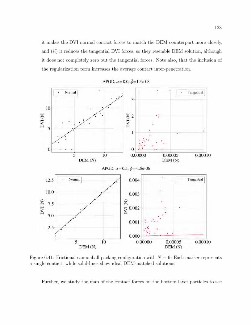
128
it makes the DVI normal contact forces to match the DEM counterpart more closely,
and (ii) it reduces the tangential DVI forces, so they resemble DEM solution, although
it does not completely zero out the tangential forces. Note also, that the inclusion of
the regularization term increases the average contact inter-penetration.
Figure 6.41: Frictional cannonball packing configuration with N = 6. Each marker representsa single contact, while solid-lines show ideal DEM-matched solutions.
Further, we study the map of the contact forces on the bottom layer particles to see

129
the effect of regularization.
Figure 6.42: Distribution of the normal force (z-direction) on the bottom particles in frictionalcannonball packing configuration with N = 6.
Figure 6.43: Distribution of the tangential force (x-direction) on the bottom particles infrictional cannonball packing configuration with N = 6.
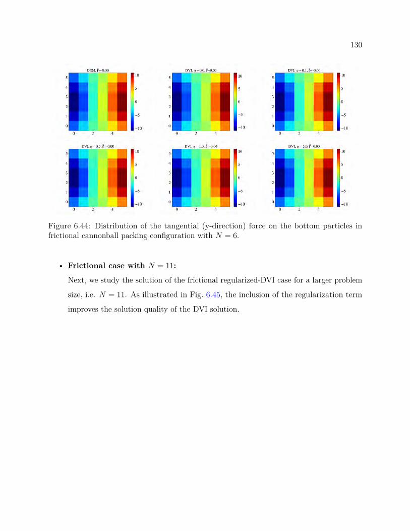
130
Figure 6.44: Distribution of the tangential (y-direction) force on the bottom particles infrictional cannonball packing configuration with N = 6.
• Frictional case with N = 11:
Next, we study the solution of the frictional regularized-DVI case for a larger problem
size, i.e. N = 11. As illustrated in Fig. 6.45, the inclusion of the regularization term
improves the solution quality of the DVI solution.

131
Figure 6.45: Frictional cannonball packing configuration with N = 11. Each marker representsa single contact, while solid-lines show ideal DEM-matched solutions.

132
Further, we study the map of the contact forces on the bottom layer particles to see
the effect of regularization.
Figure 6.46: Distribution of the normal force (z-direction) on the bottom particles in frictionalcannonball packing configuration with N = 11.
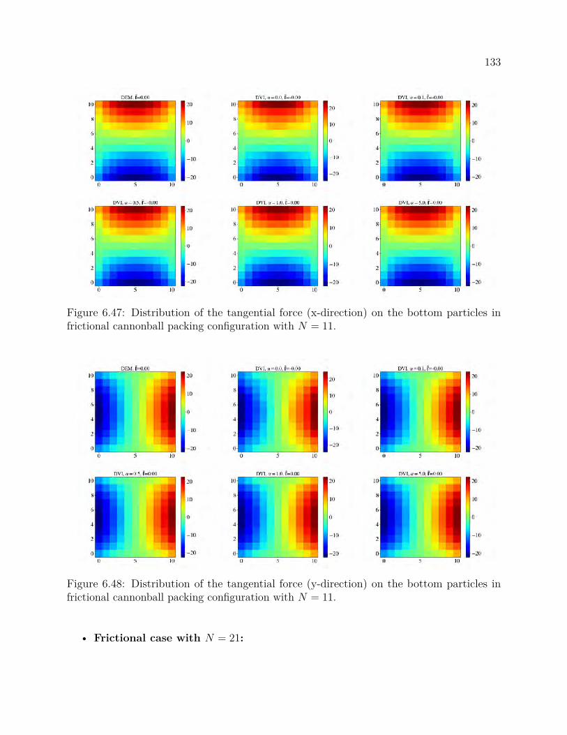
133
Figure 6.47: Distribution of the tangential force (x-direction) on the bottom particles infrictional cannonball packing configuration with N = 11.
Figure 6.48: Distribution of the tangential force (y-direction) on the bottom particles infrictional cannonball packing configuration with N = 11.
• Frictional case with N = 21:
134
Lastly, we study the solution of the frictional regularized-DVI case for a larger problem
size, i.e. N = 21. The initial results of the solution are shown in Fig. 6.49
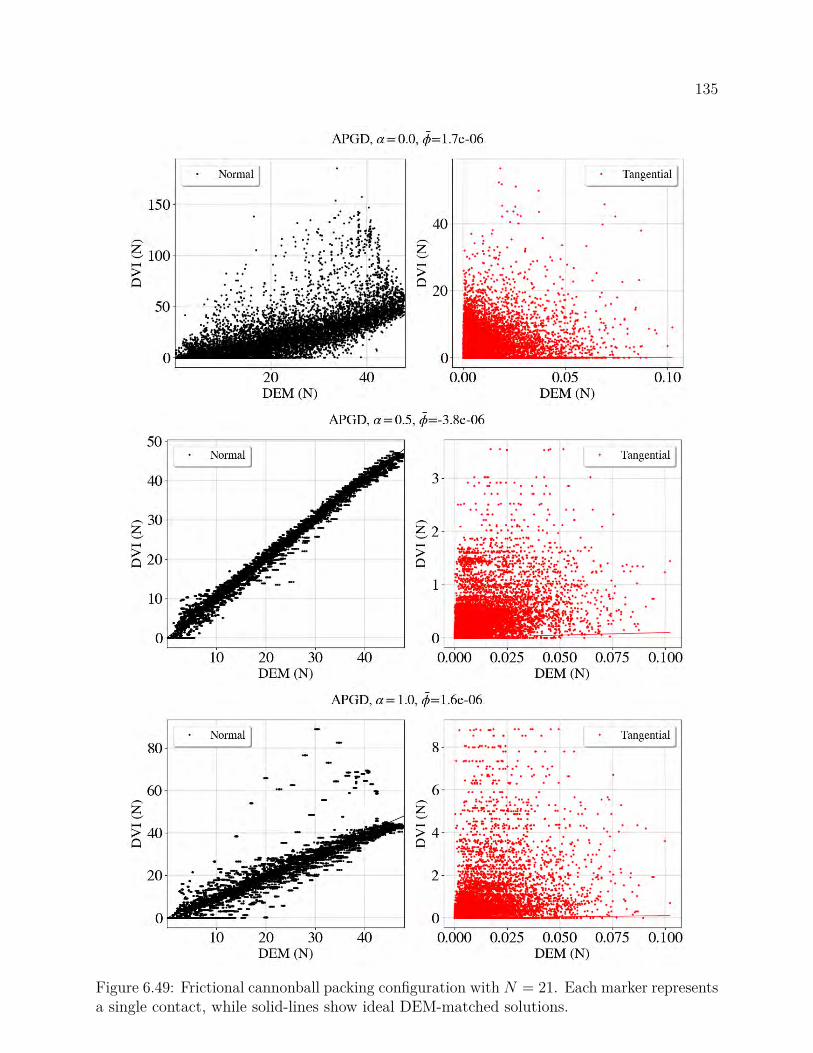
135
Figure 6.49: Frictional cannonball packing configuration with N = 21. Each marker representsa single contact, while solid-lines show ideal DEM-matched solutions.
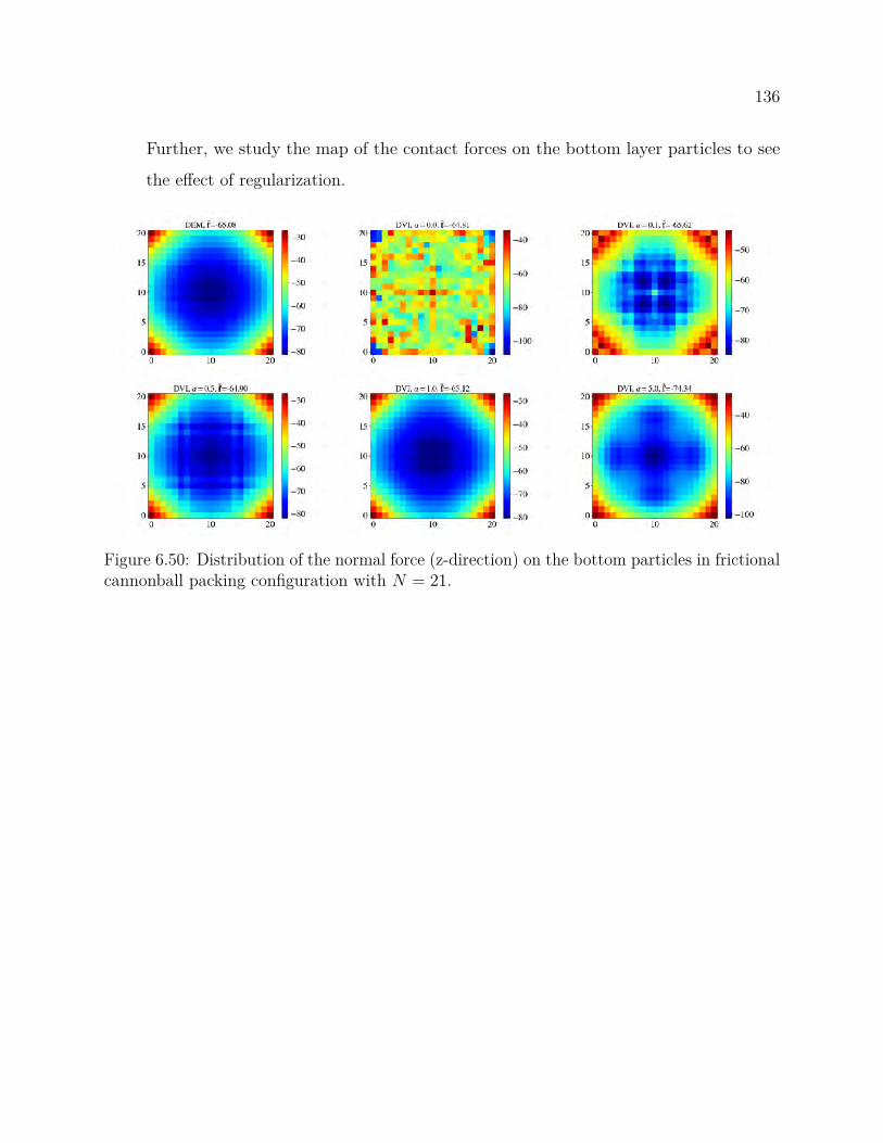
136
Further, we study the map of the contact forces on the bottom layer particles to see
the effect of regularization.
Figure 6.50: Distribution of the normal force (z-direction) on the bottom particles in frictionalcannonball packing configuration with N = 21.
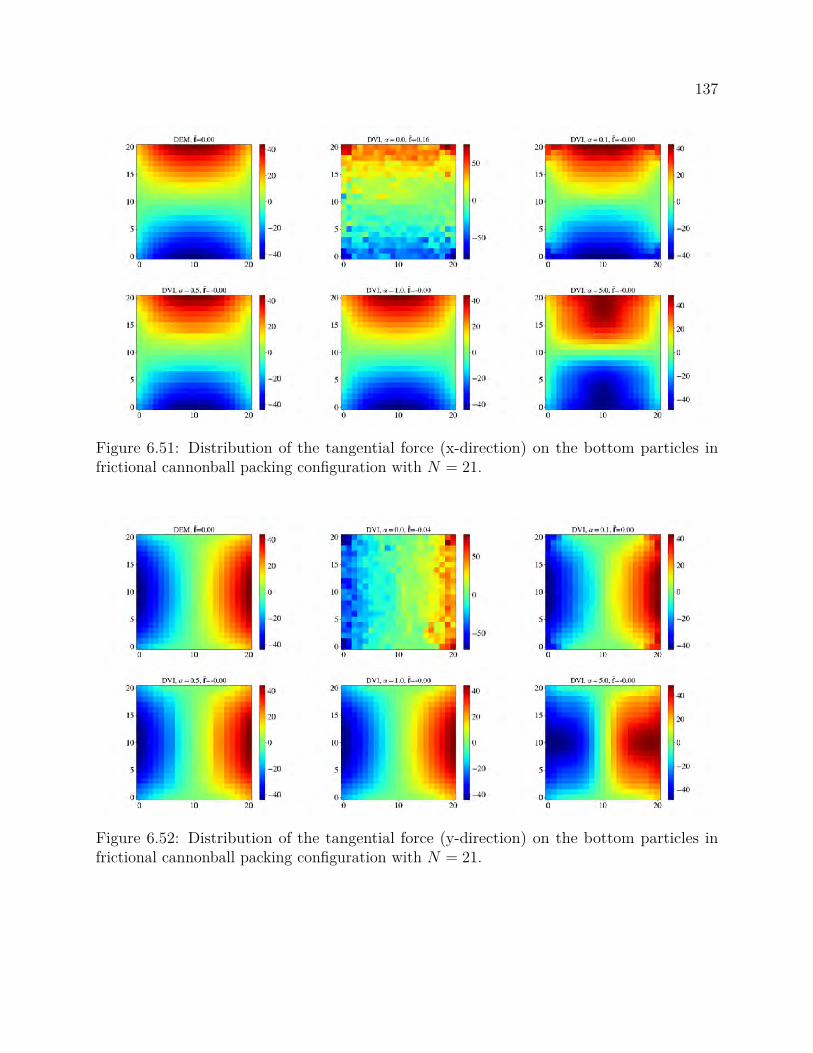
137
Figure 6.51: Distribution of the tangential force (x-direction) on the bottom particles infrictional cannonball packing configuration with N = 21.
Figure 6.52: Distribution of the tangential force (y-direction) on the bottom particles infrictional cannonball packing configuration with N = 21.

138
7 demonstration of technology
This section will demonstrate a few applications of the framework presented in this the-
sis. Applications include simulations of articular cartilage during the gait cycle, fluid-solid
interaction in complaint robotics, and continuum granular flow simulation.
7.1 Simulation of Articular Cartilage
Tibiofemoral articular cartilage withstands compressive loads of multiple times body weight
during walking, and transmits forces across skeletal joints while distributing the loading on
the underlying subchondral bone [132]. This mechanical purpose factors into cartilage health,
as normal tissue function requires homeostasis, a balance of tissue remodeling and degradation
regulated in part by the repetitive loading experienced during functional movements [133].
The substantial load-bearing capacity of this multiphase tissue is provided by the extracel-
lular matrix, a multiphase tissue composed of an ionized fluid and a solid network of collagen
fibers and embedded macromolecules. The electrostatic attraction between proteoglycan
macromolecules and the ionic fluid leads to an osmotic pressurization of the extracellular
matrix. This internal pressure is equilibrated by tensile loading in the collagen fibers. When
cartilage is loaded, the contact loads are distributed throughout the tissue via further pres-
surization of the interstitial fluid [134, 135]. This combination of interstitial fluid pressure
and compressive and shearing contact loads results in a complex loading environment for the
collagen fibers [136, 137, 138]. Characterization of this collagen fiber loading during func-
tional movement is critical to understand the superficial cartilage degradation and fibrillation
associated with the initiation of osteoarthritis [139, 140, 133, 141].
Collagen fibers exhibit distinct patterns in orientation throughout the cartilage tissue. In
the depth-wise direction, fibers extend vertically from the subchondral bone, bend through
the mid-layer and lie parallel to the articular surface in the superficial layer [142]. Within
the superficial layer, the fibers exhibit preferential orientation along the articular surface as

139
well. This superficial collagen fiber orientation is revealed through split lines produced by
inserting a needle coated in India ink into the tissue [4, 142, 143].Collagen fiber orientation
produces significant anisotropy in the tissue mechanical properties, demonstrated by increased
tensile stiffness along the split line direction [144]. Although the physiologic mechanism
linking collagen alignment to loading is still uncertain, an enzyme that selectively degrades
unloaded collagen fibers may provide this link [145, 146]. At the tissue level, the link between
loading and collagen orientation remains difficult to study, because while Magnetic Resonance
Imaging (MRI) based techniques to quantify tissue strains have recently been introduced,
they are limited in their ability to study functional movement [147, 148].
To overcome the limitations of current experimental techniques, computer simulation
is often used to investigate cartilage loading. To properly model the loading scenarios
that contribute to fiber orientation and the development of OA, simulations must resolve
the net joint loading during locomotor movements and the corresponding internal joint
tissue stresses. Simultaneous solution for the muscle forces that produce a movement and
detailed internal joint mechanics results in intractable computational complexity. As a
result, a muscle driven multibody simulation with a simplified knee model is often performed
first to determine the net joint loads, which are then used as inputs to a detailed finite
element model to solve for internal cartilage tissue stresses [149, 150, 151]. Finite element
models of cartilage of increasing complexity have been introduced including linear elastic,
multiphase, and fibril reinforced to accurately capture the response of cartilage to applied
loads [149, 152, 153]. Recently, simulation routines have been introduced that model cartilage
contact using an elastic foundation representations to allow for internal joint mechanics to be
solved simultaneously with the musculoskeletal dynamics [154, 155, 156, 157]. However, these
improved musculoskeletal simulation techniques have not been extended to resolve internal
tissue stresses.
The aforementioned simulation techniques have been used previously to gain insight into
the connection between cartilage loading and collagen orientation. Experimentally measured

140
cartilage split line orientations have been included in fiber-reinforced finite element models to
study their influence on predicted cartilage strain patterns [158, 159, 160]. Other researchers
have developed remodeling laws based on mechanical parameters such as the directions of
principal strains to predict collagen alignment [161, 162]. However, these works are limited to
simplified geometries and loading conditions and have only been applied to depth-wise collagen
orientation. Thus, it remains unknown whether cartilage split line directions correspond to
mechanical loading during locomotion.
In the preset work, a novel simulation framework which integrates kinematic and kinetic
measurements of full body movement with a muscle-driven image based model of the knee joint
to predict superficial cartilage layer mechanics was investigated. The model and simulation
framework is then used to predict cartilage surface strains due to passive osmotic pressure and
a simulated walking cycle. The orientation of the principal strains in the cartilage surface are
compared against experimentally measured split lines to provide insight into the connection
between fiber loading and orientation.
7.1.1 Computational model
This section outlines the basic ideas behind the computer implementations used to model the
geometry and deformation of the AC surfaces and their contact.
A three-body, 12 degree-of-freedom (DOF) knee model was developed from magnetic
resonance (MR) images of a healthy adult female (1.65 m, 61 kg). Details of model de-
velopment have been previously published [155], but will be briefly summarized for clarity.
Fourteen ligaments were represented by bundles of nonlinear elastic springs, with wrapping
surfaces included to prevent penetration of bony geometries. Articular cartilage surfaces were
segmented from the MR images and represented by high-resolution meshes. Cartilage contact
pressures were calculated based on the overlap depth between the articulating surfaces using
an elastic foundation model. The knee model was integrated into an existing lower extremity
musculoskeletal model [163], which included 43 muscles acting about the hip, knee and ankle
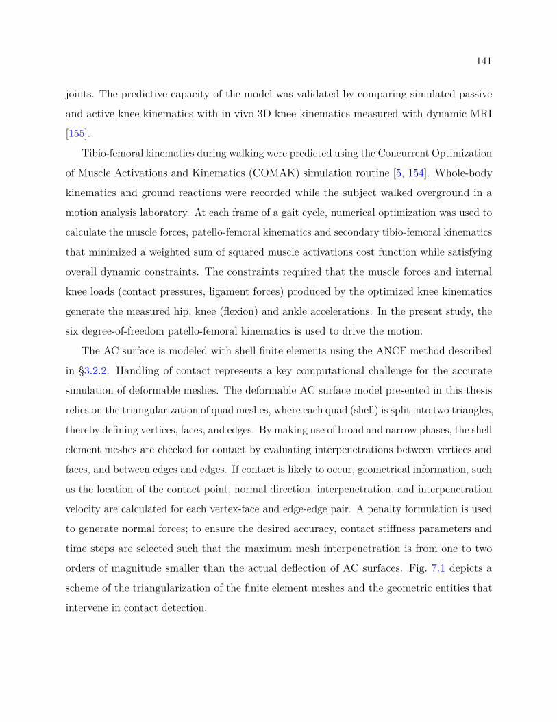
141
joints. The predictive capacity of the model was validated by comparing simulated passive
and active knee kinematics with in vivo 3D knee kinematics measured with dynamic MRI
[155].
Tibio-femoral kinematics during walking were predicted using the Concurrent Optimization
of Muscle Activations and Kinematics (COMAK) simulation routine [5, 154]. Whole-body
kinematics and ground reactions were recorded while the subject walked overground in a
motion analysis laboratory. At each frame of a gait cycle, numerical optimization was used to
calculate the muscle forces, patello-femoral kinematics and secondary tibio-femoral kinematics
that minimized a weighted sum of squared muscle activations cost function while satisfying
overall dynamic constraints. The constraints required that the muscle forces and internal
knee loads (contact pressures, ligament forces) produced by the optimized knee kinematics
generate the measured hip, knee (flexion) and ankle accelerations. In the present study, the
six degree-of-freedom patello-femoral kinematics is used to drive the motion.
The AC surface is modeled with shell finite elements using the ANCF method described
in §3.2.2. Handling of contact represents a key computational challenge for the accurate
simulation of deformable meshes. The deformable AC surface model presented in this thesis
relies on the triangularization of quad meshes, where each quad (shell) is split into two triangles,
thereby defining vertices, faces, and edges. By making use of broad and narrow phases, the shell
element meshes are checked for contact by evaluating interpenetrations between vertices and
faces, and between edges and edges. If contact is likely to occur, geometrical information, such
as the location of the contact point, normal direction, interpenetration, and interpenetration
velocity are calculated for each vertex-face and edge-edge pair. A penalty formulation is used
to generate normal forces; to ensure the desired accuracy, contact stiffness parameters and
time steps are selected such that the maximum mesh interpenetration is from one to two
orders of magnitude smaller than the actual deflection of AC surfaces. Fig. 7.1 depicts a
scheme of the triangularization of the finite element meshes and the geometric entities that
intervene in contact detection.
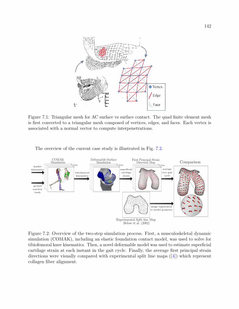
142
Figure 7.1: Triangular mesh for AC surface vs surface contact. The quad finite element meshis first converted to a triangular mesh composed of vertices, edges, and faces. Each vertex isassociated with a normal vector to compute interpenetrations.
The overview of the current case study is illustrated in Fig. 7.2.
TimeSimulationCOMAK
TimeSimulation
Deformable-Surface
Time
Direction MapFirst Principal Strain
Experimental Split line MapBelow et al. (2002)
Comparisonmarker
kinematics
ground
reaction
loads
tibiofemoral
kinematics
superficial
cartilage
strain
average
over gait
cycle
image registration
to model geometry
Figure 7.2: Overview of the two-step simulation process. First, a musculoskeletal dynamicsimulation (COMAK), including an elastic foundation contact model, was used to solve fortibiofemoral knee kinematics. Then, a novel deformable model was used to estimate superficialcartilage strain at each instant in the gait cycle. Finally, the average first principal straindirections were visually compared with experimental split line maps ([4]) which representcollagen fiber alignment.

143
Figure 7.3: Schematic comparison of the elastic foundation model (left) with the deformablemodel (right) with the 2D section views on top.
7.1.2 Results
The model is verified by comparing i) tibio-femoral contact forces and ii) deflection of the
femur and tibia cartilages obtained from the deformable-surface model against those predicted
by the rigid-surface model ([5]). The schematic comparison of the two methods is illustrated
in Fig. 7.3.
Tibio-femoral contact force patterns exhibit a characteristic double peak during stance,
with the majority of the force passing through the medial compartment. Fig. 7.4 illustrates
the comparison of the tibio-femoral contact forces predicted by the models. The time-
averaged relative difference, |x−xref ||xref |
, between the results of the present study and what has
been reported in ([5]) for the net force in the superior-inferior direction, are ≈ 19%, 27%,
for respectively medial and lateral compartments of tibia plateau and 17% for the femur
condyle. Considering the fundamental differences between the two models, the results of the
present model are in good agreement with the established approach [5] and is able to exhibit
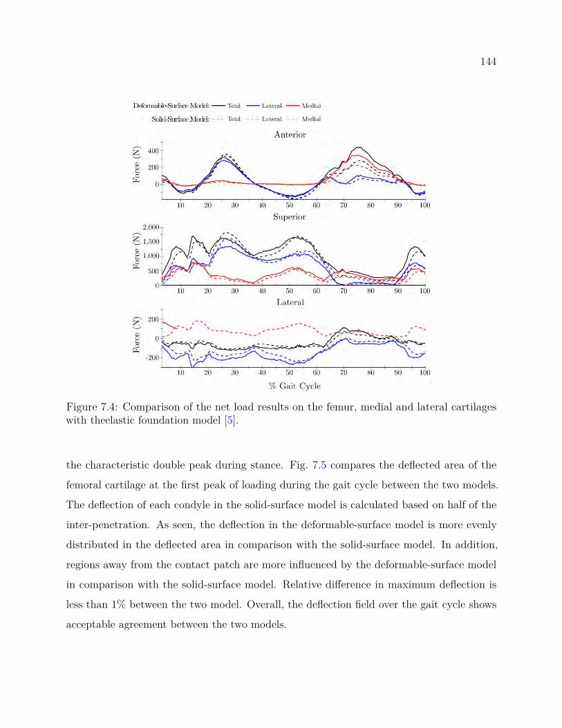
144
Figure 7.4: Comparison of the net load results on the femur, medial and lateral cartilageswith theelastic foundation model [5].
the characteristic double peak during stance. Fig. 7.5 compares the deflected area of the
femoral cartilage at the first peak of loading during the gait cycle between the two models.
The deflection of each condyle in the solid-surface model is calculated based on half of the
inter-penetration. As seen, the deflection in the deformable-surface model is more evenly
distributed in the deflected area in comparison with the solid-surface model. In addition,
regions away from the contact patch are more influenced by the deformable-surface model
in comparison with the solid-surface model. Relative difference in maximum deflection is
less than 1% between the two model. Overall, the deflection field over the gait cycle shows
acceptable agreement between the two models.

145
Elastic foundation model([5]) Deformable model
Figure 7.5: Comparison of articular cartilage inter-penetration (elastic foundation model)and deflection (deformable model). Also see Fig. 7.3
Prediction of collagen fiber orientations
The effects of two types of loading on the cartilage are investigated here: (i) internal loading
due to the cartilage internal pressure, and (ii) external loading due to the gait cycle. The
internal pressure of the cartilage is a function of the external load; as the compressive load on
the cartilage increases, the fluid content of the cartilage is reduced and the internal pressure
increases. Therefore, both effects should be investigated when studying the effect of loading on
strain distribution/directions. Moreover, considering that tibio-femoral joint predominantly
operates under the gait cycle during one’s life, it can be assumed that the gait cycle loading
and the internal pressure determine the collagen fibers’ direction. Many researchers have
correlated the maximum principal strain direction to the collagen fiber orientation (e.g. see
[4]). Hence, the deformable-surface model is used to obtain the principal strain directions for
the aforementioned scenarios.
In the first scenario, the kinematics of the gait cycle loads the cartilage and no pressure
is present. Fig. 7.6 shows the principal strain direction vectors scaled by the magnitude
146
of the principal strains at three representative instants of time during the gait cycle: Heal
strike, first peak, and second peak. During the gait cycle, the largest first principal strains, ε1,
are observed at the periphery of the cartilages, whereas, the most negative second principal
strains, ε2, are observed at the regions where the femoral cartilage undergoes larger deflection,
i.e. the central region. Due to the shape of the femoral cartilage at the medial side, the
cartilage surface undergoes compressive loading at the center of the contact region as the
principal strain of largest magnitude tends to be negative (Fig. 7.6 first peak). In order to
obtain a representative measure of principal strains over the gait cycle, the weighted principal
strain directions are averaged over time. Fig. 7.7(a) shows the split-line pattern obtained for
this case. It may be observed that the maximum (first) principal strain directions due to
external loading shows little similarities with the experimental results.
In the second scenario, only internal pressure is present. The magnitude of the applied
pressure is 0.2 MPa which is the typical hydrostatic internal pressure of the cartilage. Fig. 7.7(b)
illustrates the maximum (first) principal strain direction for this case. Comparison of the
maximum principal strain directions with experimental split-line patterns shows very good
agreement.

147
Figure 7.6: Different instants of time during the gait cycle when no internal pressure isapplied. First row: schematic of the motion during the gait cycle. Second row: deflection field.Third row: maximum principal strains. Black lines show the first principal strain directionsand are scaled by the magnitude of the first principal strain at each FE node. See Fig. 7.9 insupplementary information for corresponding tibial plateau pressures and strain patterns.
148
Figure 7.7: Comparison of the fiber alignment predicted by this study for different scenarioswith experimental results [4] on the femur condyle. Histograms demonstrate the distributionof the angle of deviation between the experimental split lines and predicted principal straindirections. The dashed lines on histograms show the median angle of deviation. See Fig. 7.9 insupplementary information for simulated first principal strain directions on the tibial plateau.
149
Figure 7.8: Different instants of time during the gait cycle when no internal pressure isapplied. First row: schematic of the motion during the gait cycle. Second row: deflectionfield. Third row: maximum principal strains (black lines show the maximum principal straindirections and are scaled by the magnitude of the principal strain at each FE node.
150Medial L
ateral
Posterior
Anterior
(a) Gait cycle (b) Internal pressure (c) Gait cycle + Internal pressure
Figure 7.9: Comparison of the average first principal strain directions induced via (a)tibiofemoral loading during gait, (b) internal pressure and (c) coupled gait loading andinternal pressure.
Finally, both scenarios can be combined in one simulation in order to see whether one
of them dominates the other or both scenarios equally affect the split-line pattern (see
Fig. 7.7(c)). The comparison between Fig. 7.7(a) and Fig. 7.7(c) shows that, for the selected
internal pressure level, the maximum principal strain is dominated by the gait cycle simulation.
The lower the internal pressure, the smaller the resulting principal strains and the smaller
contribution to the total split-line pattern. Conversely, with the application of larger internal
pressures, the magnitude of the principal strain becomes dominant; therefore, Fig. 7.7(c)
would become closer to Fig. 7.7(b).
7.1.3 Discussion
The methodology used in the present study differs from the rigid-surface approach, the
prevalent method that is used to resolve the internal joint loads in AC along with the
musculoskeletal dynamics [5, 155, 156, 157]. In the solid-surface model, the deformation for
each element is independent of neighboring elements and is simply approximated according to
inter-penetration of two solid surfaces representing articular surfaces. The solid-surface model

151
has been shown [157, 164] to be able to predict the contact pressure fairly well when compared
to FE models, but it essentially does not resolve the internal tissue stresses. In contrast, the
deformable-surface model captures the deformation of the articular surface and consequently
allows for studying the tissue level stresses and mechanical behavior of the superficial region
of the AC in more details. Therefore, properties such as strain directions, which are of interest
in the current study, can be captured using this method. The higher-fidelity method, however,
comes at a higher computational cost in comparison to the solid-surface model.
Moreover, the modeling technique used in the present work removes a number of the
limitations of previous studies. Previously, remodeling laws were used in an attempt to
characterize the collagen fibers direction, but only simplified loading scenarios and simplified
geometries [161] and depth-wise orientation of fibers [162] were investigated. In the present
study, principal directions on AC surface were investigated for the actual geometry of the
articular surface and during the gait motion. Overall, this study improves our understanding
of how the collagen fibers orientation is directed by the mechanical conditions at the surface
of the articular cartilage, which is of interest in areas such as tissue-engineering.
The results obtained from the current study suggest that depending on the type of the
mechanical loading applied on articular surface, different predicted patterns for collagen fibers
will emerge. Among these types of loading, the patterns we obtained due to the internal
pressure more closely match the experimental results. This suggests that the surface-wise
collagen fibers alignment might be tied to internal loads. Nonetheless, the external loadings
such as gait motion can still indirectly affect the split-line patterns by increasing the internal
pressure of the articular cartilage. See [10] for more details about this model.
7.2 Continuum Simulation of Granular Flows
In large, rigid multibody dynamics problems with friction and contact, encountered for
instance in granular flows, one can witness distinctly different system-level dynamics. This
section concentrates on the case of fluid-like behavior of large multibody dynamics systems
152
such as granular materials, when the system experiences large strains. The results reported
herein draw the Newton-Euler equations discussed in section §3.1 for capturing the dynamics
of granular flows in a discrete sense. In the continuum sense, the modeling approach discussed
in in sections §4.2.1-§4.2.3 is employed. To demonstrate the similarities and differences
between the multibody and fluid dynamics we consider three problems modeled and solved
using different methods; (i) a compressibility test; (ii) the classical dam break problem,
and (iii) the dam break simulation with an obstacle. These experiments provide insights
into conditions under which one can expect similar characteristics from multibody and fluid
dynamics systems governed by manifestly different equations of motion and solved by vastly
different numerical solution methods.
Herein, dynamics of spheres of identical radii is captured via the Discrete Element Method
(DEM). In this approach, the time evolution of the rigid sphere i is expressed as
mdvidt
= mfi +∑i6=j
(Fijn + Fij
t
), (7.1a)
where
Fijn = f
(δij
2R
)(knδ
ijnij − γnmvijn), and (7.1b)
Fijt = f
(δij
2R
)(−ktuijt − γtmvijt
), (7.1c)
are, respectively, the normal and tangential contact forces; kn and kt indicate stiffnesses;
and γn and γt are damping coefficients for the normal and tangential directions, respectively.
Above, m is the mass of particles, m is an effective mass, vi is the velocity of particle i, δij
represents the mutual deformation of two elements in contact, and fi represent an external
force density such as gravity (g).
Once all contact forces and resultant accelerations are computed for timestep k, the latter
are numerically integrated to yield the new velocity and position at timestep k + 1. Different
153
choices of time-integration methods [124] such as Explicit Euler, Extended Taylor, and a
second-order integrator proposed by Chung [165] are possible. The latter integrator assumes
the formvk+1 = vk + ∆t
(32ak −
12ak−1
)xk+1 = xk + vk∆t+ (∆t)2
(βak +
(12 − β
)ak−1
).
(7.2)
It draws on a multistep approach, providing second-order integration for both position and
velocity and strong numerical damping. On the down side, the Chung approach requires the
caching of previous accelerations ak−1, increasing the memory overhead. It also provides β as
a tunable parameter for the integrator’s numerical damping, with the stability requirement
that 1 ≤ β ≤ 2827 .
7.2.1 Bucket of Material
In this benchmark test we consider a bucket filled up with material – in one case fluid, and
granular material in a second case. We compare the magnitude of the average force on the
side walls of the container for both media. This averaged force changes vertically. For the
fluid media, there exists an analytical solution that comes from the hydrostatic fluid state.
According to hydrostatic fluids, the pressure distribution is linear across the depth of the
bucket – the larger the depth, the higher the force impressed on the wall. Consequently, it
is easy to show that the averaged pressure (normal) force on each side of the container is
ρgh2L/2, where h is the depth of the fluid in the bucket and L is the length of side wall.
Furthermore, the ratio of this force to the weight of the material in the bucket for a LxLxh
fluid domain is rf = h/2L. We performed DEM simulation to evaluate this ratio for a
granular media instead of a fluid media. We calculate this ratio in granular material according
to rg = |Fn|Mg
, where |Fn| is the averaged normal forces across the side walls of the container,
M is the total mass of the system, and g is the gravity. Finally, we calculate the relative
error according to e = rf−rg
rf× 100. As shown in Fig. 7.10, the relative error is considerably
small for the h values that were simulated for a bucket of material with L= 1m.
154
Figure 7.10: The relative error of dimensionless normal force experienced by the side wallsof a bucket of material for different height (h) of material. The relative error is calculatedaccording to e = rf−rg
rf× 100, where rf is the non-dimensional averaged fluid normal force
and rg is the non-dimensional averaged granular normal force on the side walls. The rg iscalculated from the DEM simulation while rf is computed from hydrostatic fluids.
We hypothesize that there should be a perfect agreement between the two media for this
test and attribute the relative error seen in Fig. 7.10 to mainly two factors: (i) numerical
errors of the DEM simulations; and (ii) numerical errors associated with approximating the
height of the granular material bucket from the particles’ information. It is important to note
that the DEM simulations were performed with frictionless monodisperse spherical particles.
We emphasize that rg is different for frictional particles. A detailed discussion on the interplay
between the friction forces and the side walls, as well as on the sensitivity of the results with
respect to the particles’ shape goes beyond the scope of this contribution and is the subject
of ongoing work and goes beyond the scope of the current thesis.
155
7.2.2 Material Column Collapse
The initial domain of the material is 2mx4mx2m, while 6mx4mx4m is the size of the container.
The reference density is ρ = 1000 kg/m3, and the gravity of g = −9.8 m/s2 is applied in the
y direction.
We study the propagating wave front both in granular material flow and the fluid flow.
We highlight the similarities in terms of front speed as shown in Fig. 7.11, and the differences
in terms of the two characteristics of the dam break simulation, i.e. the roll up and the second
splash [9] as shown in Fig. 7.12.
Figure 7.11: Comparison of the front position in the dam break simulated with DEM andCFD.

156
Figure 7.12: Comparison of the roll up (left) and the second splash (right) instances of thedam break simulation between granular (bottom) and fluid (top) mediums.
Considering that the CFD and the DEM solvers solved different governing equations,
the similarity that is seen in terms of front propagation position is somewhat perplexing.
However, as shown in Fig. 7.11, the front position predicted by the DEM simulation moves
slightly slower than the one predicted by the CFD solver. We attribute this discrepancy to
the bulk density of the material; applying ρ = 1000 kg/m3 to individual grains results in
smaller overall density in granular material. This is true because of the nature of the packing
in granular material, which allows for empty spaces between the grains. This feature, for
example, guarantees that a bucket of sand is lighter than a bucket of fluid, assuming that
the density of grains is equal to density of the fluid and the buckets have similar dimensions.
Hence, we hypothesize that the slower front speed is due to lighter material in DEM simulation.
On the CFD side only, a more ample discussion of this test may be found in [96, 9].

157
7.2.3 Column Collapse with an Obstacle
In this experiment we placed a rigid cylindrical obstacle in front of the dam and monitor the
overall force experienced by the cylinder over time after the dam breaks. The configuration of
the problem is as follows: 2mx4mx2m is the initial domain of the material, and 6mx4mx4m
is the size of the container. The dam is place in the leftmost corner of the domain and a 4
meter tall cylinder with the radius of 0.3m is placed at x = 5m from the leftmost side of
the container. Figure 7.13 demonstrates the force experienced by the cylinder for both the
granular and the fluid material for different fluid’s viscosities, and different grains diameter.
As shown in Fig. 7.13, within the simulated range, the viscous forces in the fluid simulation
do not play a major role in the overall force on the cylinder. Similarly for granular flow, the
force exerted on the cylinder is virtually insensitive to the particles’ diameter.
Figure 7.13: Comparison of the normalized horizontal force experienced by the cylinder in thedam break simulation for different viscosities of the fluid and for different particle diametersof the granular media.
Assuming insignificant viscous contribution due the large Re observed in this problem,
the fluid flow represents a momentum balance between the inertia, gravity, and pressure

158
forces (see Eq. 4.33). As highlighted in Fig. 7.13, we can consider two different stages in the
simulation. Region 1 : in this stage, good agreement is observed between the two media. We
hypothesize that this is true because of the dominant effects of the inertia over the pressure
forces. Due to the large value of the velocity, the Euler number (Eu = p0ρ0u2
0) is relatively
small, diminishing the contribution of the normal stress (pressure). Region 2 : the agreement
between the two media is gradually vanishing because of the different nature of normal forces
in granular media compared to pressure gradient forces in fluid flow. This is due to the
reduction of the inertia forces and the consequent augmentation of the pressure forces, as can
be understood from the Eu number. In Fig. 7.14 snapshots of the fluid and granular flow
simulations are shown for a qualitative comparison of the time evolution of the two media.
Figure 7.14: Snapshots of the fluid (top) and the granular material (bottom) simulation ofthe dam break with a cylindrical obstacle at t=1s (left), t=2s (middle), t=2.75s(right).
7.2.4 Discussion
Through numerical simulation of the underlying physics, we presented comparisons between
the granular and the fluid flows for three experiments. Using an adimensionalization of the
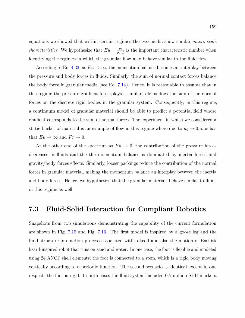
159
equations we showed that within certain regimes the two media show similar macro-scale
characteristics. We hypothesize that Eu = p0ρ0u2
0is the important characteristic number when
identifying the regimes in which the granular flow may behave similar to the fluid flow.
According to Eq. 4.33, as Eu→∞, the momentum balance becomes an interplay between
the pressure and body forces in fluids. Similarly, the sum of normal contact forces balance
the body force in granular media (see Eq. 7.1a). Hence, it is reasonable to assume that in
this regime the pressure gradient force plays a similar role as does the sum of the normal
forces on the discrete rigid bodies in the granular system. Consequently, in this regime,
a continuum model of granular material should be able to predict a potential field whose
gradient corresponds to the sum of normal forces. The experiment in which we considered a
static bucket of material is an example of flow in this regime where due to u0 → 0, one has
that Eu→∞ and Fr → 0.
At the other end of the spectrum as Eu → 0, the contribution of the pressure forces
decreases in fluids and the the momentum balance is dominated by inertia forces and
gravity/body forces effects. Similarly, looser packings reduce the contribution of the normal
forces in granular material, making the momentum balance an interplay between the inertia
and body forces. Hence, we hypothesize that the granular materials behave similar to fluids
in this regime as well.
7.3 Fluid-Solid Interaction for Compliant Robotics
Snapshots from two simulations demonstrating the capability of the current formulation
are shown in Fig. 7.15 and Fig. 7.16. The first model is inspired by a goose leg and the
fluid-structure interaction process associated with takeoff and also the motion of Basilisk
lizard-inspired robot that runs on sand and water. In one case, the foot is flexible and modeled
using 24 ANCF shell elements; the foot is connected to a stem, which is a rigid body moving
vertically according to a periodic function. The second scenario is identical except in one
respect: the foot is rigid. In both cases the fluid system included 0.5 million SPH markers.

160
The simulation time step was chosen such that CFL=0.1 via Eq. (4.113). This example was
run on a GTX 1080 Nvidia GPU and took 15 hours of runtime for a 30 second-long simulation
of the FSI problem in the presence of a deformable foot. A similar simulation demonstrating
the hydrodynamic buoyancy of a wedged-shape plate is shown in Fig. 7.16.
(a) Flexible Fin (b) Rigid Fin
Figure 7.15: Snapshots of the simulation of a fin slapping on the surface of water. (See [6]Movie #137 for the animation)
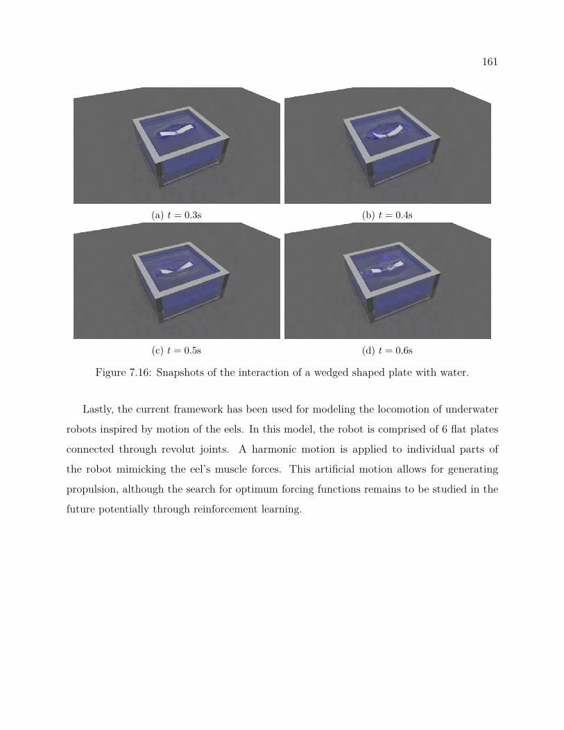
161
(a) t = 0.3s (b) t = 0.4s
(c) t = 0.5s (d) t = 0.6s
Figure 7.16: Snapshots of the interaction of a wedged shaped plate with water.
Lastly, the current framework has been used for modeling the locomotion of underwater
robots inspired by motion of the eels. In this model, the robot is comprised of 6 flat plates
connected through revolut joints. A harmonic motion is applied to individual parts of
the robot mimicking the eel’s muscle forces. This artificial motion allows for generating
propulsion, although the search for optimum forcing functions remains to be studied in the
future potentially through reinforcement learning.

162
Figure 7.17: Fluid-solid interaction in the context of locomotion of bio-inspired under-waterrobots.
More example animations for illustration of the current framework are available at [6],
movie #126, #133, #134, #137, #138, #165, and #168.
163
8 conclusions
In this thesis, the numerical modeling and simulation of multi-physics mechanical systems
consisting of discrete and continua were investigated via Lagrangian methods. Specifically,
(a) Rigid and flexible multi-body dynamic systems featuring frictional contact were studied.
The former was employed in granular material simulations while the later was used in
the simulation of articular cartilage during the gait cycle.
(b) The dynamics of continua were investigated for fluid dynamics problems and for continuum
simulation of granular flows. The continuum modeling of granular flows allowed for
modeling such materials via a computationally less expensive method than the DEM
counterpart.
(c) The coupling between continuum and discrete sub-systems was investigated primarily for
fluid-solid interaction problems.
The HPC approach employed in this thesis draws on hybrid multi-core shared memory
architecture for discrete systems and GPU computing for the continua. The software im-
plementation of the framework is part of an open-source software and is available on public
domains.
Verification and validation of the different aspects of the numerical method were con-
ducted through comparison with experimental results or other well-established numerical
methods. The multi-physics framework was used in studying real-world problems, including
(i) the relation between loading and the articular cartilage split-line patterns, (ii) fluid-solid
interaction in compliant and under-water robotic applications, and (iii) continuum modeling
of granular material.
The developments made as part of this thesis work provide a robust foundation for coupling
rigid bodies, fluids and flexible objects in a fully Lagrangian framework. Traditional Eulerian
approaches for such multi-physics coupling involve tracking implicit surfaces through the
164
continuum or re-meshing the domain frequently throughout the simulation. The Lagrangian
alternative proposed in this work is more robust for multi-physics problems that involve large
displacement and deformation in the discrete system.
The specific contributions of the author are summarized as follows:
• Investigated the use of SPH for the Navier-Stokes equations
– Investigated four different SPH methods (WCSPH, ISPH, KCSPH, and IISPH)
and their solution attributes
– Performed a comparison between Implicit SPH (ISPH), Weakly Compressible SPH
(WCSPH), and Kinematically Constrained SPH (KCSPH)
– Compared and contrasted the solution attributes of SPH as a Lagrangian method
against continuous finite element method for free-surface and fluid-solid interaction
problems
– Implemented and improved the Implicit Incompressible SPH [14] method by solving
the discretized Poisson pressure equation via advanced linear solvers
– Implemented and validated a projection-based implicit, both velocity and pressure,
solver that can handle a wide range of fluid flows ranging from highly viscous flows
to flows with moderately large Reynolds numbers in the laminar regime
– Investigated the use of consistent SPH discretization for internal flow problems
– Implemented the Herschel-Bulkley fluid model for modeling and simulation of
non-Newtonian fluids
– Investigated the use of ISPH method for modeling and simulation of granular
dynamics as a non-Newtonian fluid
• Investigated the solution quality in frictional-contact problems and demonstrated insights
gained in the context of a biomechanics application
– Investigated the use of the Tikhonov regularization method for imparting unique-
ness to the distribution of frictional contact forces in granular dynamics problems
solved via a differential variational inequality approach

165
– Simulated the tibiofemoral cartilage contact during walking for the prediction of
collagen fiber orientation
• Developed a partitioned fluid-solid interaction framework
– Coupled the fluid solver to a multi-body engine capable of simulating rigid and
flexible bodies interacting through frictional contact
– Validated the fluid-structure coupling via benchmark experiments featuring flexible
and rigid elements
• Leveraged hybrid CPU/GPU parallelization to improve the performance of the FSI
framework
– Implemented SPH on GPU cards using CUDA to leverage high memory bandwidth
– Implemented Krylov linear solvers such as GMRES and BiCGStab on GPU to
improve the efficiency of the underlying linear solvers
– Leveraged OpenMP for parallelism of the flexible multi-body dynamics solver on
the CPU
– Improved the efficiency of the low-level matrix operation on the host code via AVX
vectorization intrinsics
8.1 Statement of Acknowledgment
This work was supported by National Institutes of Health [grant number EB015410] and
National Science Foundation [grant number CMMI 1635004]. The development of the multi-
physics platform discussed in this thesis employed the work of previous authors as follows:
• The WCSPH formulation discussed in §4.4.2 adopt the implementation of the previous
work discussed in [166].
• The KCSPH formulation discussed in §4.4.5 employed the implementation of the
previous work discussed in [167].
166
• The multi-body and the rigid body formulation discussed in §3.1 and §3.2 employed
Chrono [102, 168].
• The development of the articular cartilage model discussed in §7.1 was conducted
in collaboration with the co-authors of the paper published in [10]. Tibio-femoral
kinematics during walking explained in §7.1.1 employed the data published in [5, 154].
8.2 Future Direction of Research
The future directions of research involve solving more challenging real-world problems with
the current framework as well as improving the numerical methods employed in this work.
Details are provided in the next three subsections.
8.2.1 Hybrid Eulerian-Lagrangian Discretization: MPM
Material Point Method (MPM) is a hybrid Eulerian-Lagrangian discretization that can be
used to space-discretize a wide range of problems from fluids to solids. MPM was first
described in [169], and is a derivative of the fluid-implicit-particle (FLIP) method [170], which
is based on the particle-in-cell (PIC) method [171]. The key idea of MPM is to store the
state variables on Lagrangian material points, while the equations of motion are solved on a
background grid. More specifically, in MPM the body is discretized with a set of material
points placed on a background grid, which is used for computation of the gradient terms.
Some of the problems associated with mesh-based methods for FSI applications (see §2.3) are
not encountered in MPM; this is because the re-meshing step is not necessary, making MPM
suitable for modeling problem involving large deformations. At the beginning of the MPM
simulation, the grid is initialized such that it includes the continuum body. The material
points are distributed on the continuum body as well. During each time-step, the MPM
algorithm can be summarized in the following steps:
167
1. Quantities such as mass, velocity, internal and external forces are extrapolated from
the material points to the grid nodes using the shape functions as:
φinode =∑
p∈S(node i)φpmpNmp−nd(xip), (8.1)
where Nmp−nd(xip) is the interpolation function from the material points to the grid
nodes.
2. Equations of motion with proper constitutive relations are solved on the grid for velocity
and acceleration. The mesh nodes are advected and required gradients are calculated
on the grid.
3. Grid node quantities are extrapolated back to the material points according to
φpmp =∑
i∈S(node p)φimpNnd−mp(xpi), (8.2)
where Nnd−mp(xpi) is the interpolation function from the grid nodes to the material
points.
4. The distorted grid is reseted to a uniform grid encompassing the continuum body for
the next time step.
8.2.2 Higher-order Lagrangian Discretization: GMLS
SPH is a robust mesh-less method for a wide range of problems, especially for fluid-solid
interaction problems involving large displacement and deformation. However, instability/ac-
curacy concerns are associated with each of the SPH methods discussed in sections §4.4
at high/low Reynolds numbers. The idea behind the Generalized Moving Least Squares
method is to reconstruct a function from an unstructured set of point data sampled in a
neighborhood of any point in space. Specifically, if the function ψ(x) is to be approximated
168
by a mth-order polynomial from its point data values ψj in some neighborhood of x, the
GMLS approximation of ψ(x) is as follows:
ψ(xi) = P Ti (xi)c∗i , (8.3)
where c∗i is the unknown polynomial coefficient vector that is obtained through minimization of
a weighted residual functional, e.g., ∑j∈S(i)
(ψj−P T
i (xj)ci)2Wij . Above, P is the polynomial
basis vector, e.g., P = [1, x, y, x2, xy, y2] in 2D for m = 2, which introduces 6 unknowns in
the coefficient vector c∗i . After taking the variation with respect to ci, it follows that:
c∗i = M−1i
( ∑j∈S(i)
Pi(xj)Wijψj
), (8.4)
where
Mi =∑j∈S(i)
Pi(xj)WijPTi (xj). (8.5)
The GMLS procedure introduces a way for optimal recovery of linear target functionals over
a desired reproduction space. See [20, 19] for more details about this method.
8.2.3 Biomechanics Applications: Articular Cartilage
Osteoarthritis (OA), the breakdown of the articular cartilage, affects the lives of millions of
adults. Although there are treatments to manage the condition, there is no cure nor any
completely effective method of preventing the disease. As such, it is essential to comprehen-
sively study factors that contribute to OA in order to guide the development of improved
treatments. Research in this field has the potential to substantially improve our understanding
of multi-scale articular cartilage mechanics, which assists efforts to investigate degenerative
pathways. The focus of this direction of future research is on the modeling and simulation of
the micro-structure of the articular cartilage.
Structurally, cartilage consists of two distinct phases: a fluid phase, composed of water and
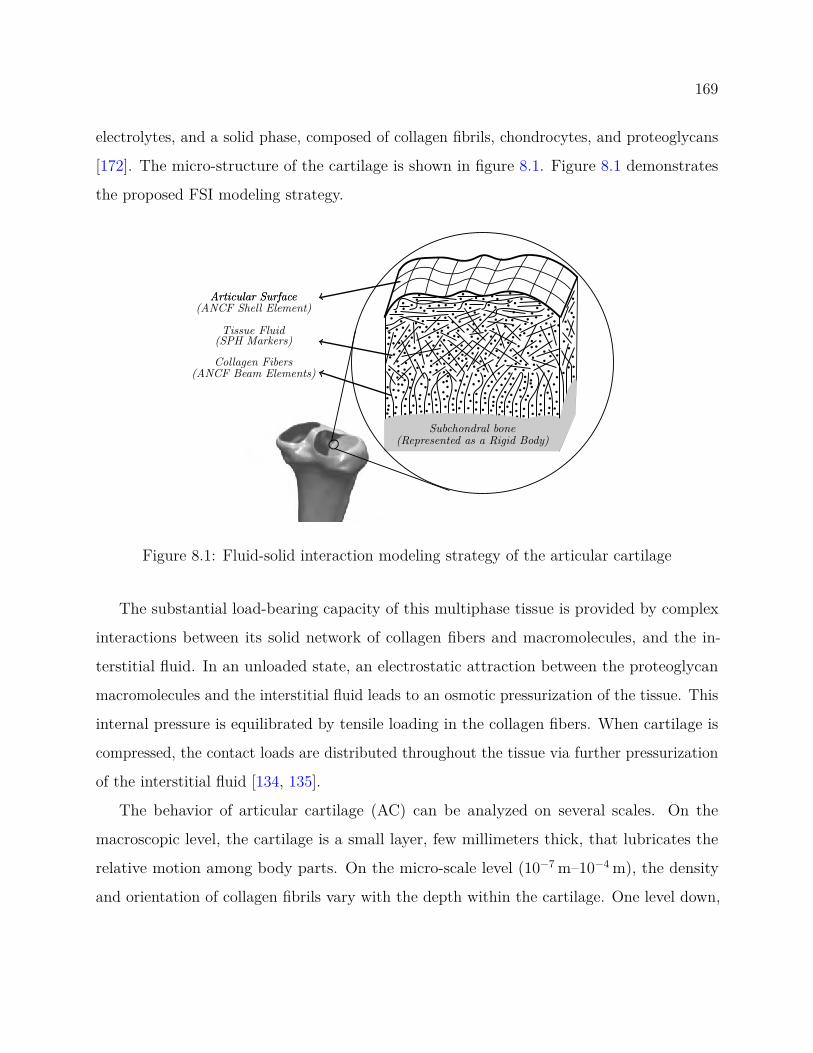
169
electrolytes, and a solid phase, composed of collagen fibrils, chondrocytes, and proteoglycans
[172]. The micro-structure of the cartilage is shown in figure 8.1. Figure 8.1 demonstrates
the proposed FSI modeling strategy.
a
b
b
b bb
b
b
b
b
bb
bb
b
b
b
b
bb
b
b
b
bb
b
b
bb
b
b
b
b
b
b
b
b
b
b
bb
b
b
bb
b
bb
b
b
b
b
b
bb
b
b
bb
b
b
bb
bb
b
b
b
b
b
bb
b
bb
b
bbb
bb
b
b
b
bbb b
b
bb
b
b
b
b
b
b
b
b b
b
b
b
bb
b b
b
b
b
b
b
b
b b
b
b
bbb
bb
b
b bb
bbbbb
b
bbb
bb
b
bbb
bbbbb
bb b
bbbb
bb
bbb
bb b
b
b
b
b
b
b
b
b
b
b
b
b
b
b
b
b
b
b bb
b
b
b
bb
b
b
b
bb
bb
b
b
b
b
bb
b
bb
b
b
bb
b
b
b
b
b
bb
b
b
bbb
b
b
b
b
bb
b
b
bb
b
b
b
bb
bb
b
b
b
b
b
bb
bb
b
b
bb
bb
b
bbb
bbb
b bb
bb
b
bb
b
bb
b
b
b
bb
b
b
b
b
bb
b
b
b
b
bb
b
bb
bbb
bbb
bb
b
b
b
b bb
b
b
b
b
b
b
b
b
b
bb
b
b
b
b
b
b
b
b
b b
b
b
b
b
b
b
b
b
b
b
Subchondral bone(Represented as a Rigid Body)
Articular SurfaceArticular Surface(ANCF Shell Element)
Tissue Fluid(SPH Markers)
Collagen Fibers(ANCF Beam Elements)
Figure 1: FSI representation of the articular cartilage
1
Figure 8.1: Fluid-solid interaction modeling strategy of the articular cartilage
The substantial load-bearing capacity of this multiphase tissue is provided by complex
interactions between its solid network of collagen fibers and macromolecules, and the in-
terstitial fluid. In an unloaded state, an electrostatic attraction between the proteoglycan
macromolecules and the interstitial fluid leads to an osmotic pressurization of the tissue. This
internal pressure is equilibrated by tensile loading in the collagen fibers. When cartilage is
compressed, the contact loads are distributed throughout the tissue via further pressurization
of the interstitial fluid [134, 135].
The behavior of articular cartilage (AC) can be analyzed on several scales. On the
macroscopic level, the cartilage is a small layer, few millimeters thick, that lubricates the
relative motion among body parts. On the micro-scale level (10−7 m–10−4 m), the density
and orientation of collagen fibrils vary with the depth within the cartilage. One level down,

170
on the ultra-scale (10−8 m–10−6 m), proteoglycans and individual collagen fibrils of up to
200 nm in diameter interact electrostatically and mechanically.
The mechanics of AC has been modeled in the literature through continuum-based representa-
tions using either biphasic or triphasic formulations, relying on constitutive properties derived
from experimental observations [173, 174]. These formulations use the methods of composite
materials for giving directional properties to the cartilage. While these approaches provide a
holistic view of the tissue, they do not explicitly model the discrete fluid-solid interactions
(FSI) on the ultra-scale level. The future investigation involves an FSI approach to model
the microstructure of the articular cartilage using the fundamental elements described above.
Modeling articular cartilage on the ultra-scale level through a discrete, fully coupled repre-
sentation of fluid and solids provides more accurate insight into the biomechanical properties
of the AC. This direction of future research allows for deepening our understanding of how
macroscopic behavior is affected by the interplay of microstructural elements. Preliminary
results of the small-scale FSI model for a confined compression test are demonstrated in
Figure 8.3.
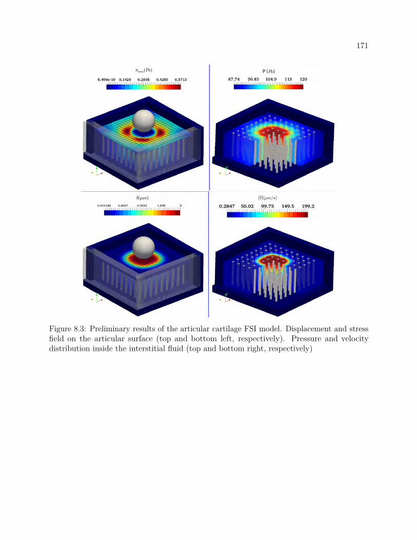
171
Figure 8.3: Preliminary results of the articular cartilage FSI model. Displacement and stressfield on the articular surface (top and bottom left, respectively). Pressure and velocitydistribution inside the interstitial fluid (top and bottom right, respectively)
172
bibliography
[1] K. Ragui, A. Boutra, R. Bennacer, and Y. K. Benkahla, “Progress on numericalsimulation of yield stress fluid flows (part i): Correlating thermosolutal coefficients ofbingham plastics within a porous annulus of a circular shape,” International Journalof Heat and Mass Transfer, vol. 126, pp. 72–94, 2018.
[2] C. Antoci, M. Gallati, and S. Sibilla, “Numerical simulation of fluid–structure interactionby SPH,” Computers and Structures, vol. 85, no. 11, pp. 879–890, 2007.
[3] A. J. Crespo, J. M. Domínguez, B. D. Rogers, M. Gómez-Gesteira, S. Longshaw,R. Canelas, R. Vacondio, A. Barreiro, and O. García-Feal, “DualSPHysics: Open-sourceparallel CFD solver based on Smoothed Particle Hydrodynamics (SPH),” ComputerPhysics Communications, vol. 187, pp. 204–216, 2015.
[4] S. Below, S. P. Arnoczky, J. Dodds, C. Kooima, and N. Walter, “The split-line patternof the distal femur: A consideration in the orientation of autologous cartilage grafts,”Arthroscopy, vol. 18, no. 6, pp. 613–617, 2002.
[5] R. Smith, K. Choi, D. Negrut, and D. G. Thelen, “Efficient computation of cartilagecontact pressures within dynamic simulations of movement,” Computer Methods inBiomechanics and Biomedical Engineering: Imaging and Visualization, no. March, 2016.
[6] Simulation-Based Engineering Lab (SBEL), “Movies, Physics-Based Modeling andSimulation.” http://sbel.wisc.edu/Animations. Accessed: 2018-06-09.
[7] M. Rakhsha, L. Yang, and D. Negrut, “A comparison of three SPH methods for thesolution of the fluid-solid interaction problem,” Computer Methods in Applied Mechanicsand Engineering - under review, 2019.
[8] M. Rakhsha, Y. Yang, C. Kees, and D. Negrut, “Lagrangian vs. Eulerian: An analysisof two solution methods for free-surface flows and fluid solid interaction problems,”Under Review, 2019.
[9] M. Rakhsha, A. Pazouki, R. Serban, and D. Negrut, “Using a half-implicit integrationscheme for the SPH-based solution of fluid-solid interaction problems,” ComputerMethods in Applied Mechanics and Engineering, vol. 345, pp. 100–122, 2019.
[10] M. Rakhsha, C. R. Smith, A. M. Recuero, S. C. Brandon, M. F. Vignos, D. G. Thelen,and D. Negrut, “Simulation of surface strain in tibiofemoral cartilage during walkingfor the prediction of collagen fibre orientation,” Computer Methods in Biomechanicsand Biomedical Engineering: Imaging & Visualization, vol. 7, no. 4, pp. 396–405, 2019.

173
[11] H. Mazhar, A. Pazouki, M. Rakhsha, P. Jayakumar, and D. Negrut, “A differentialvariational approach for handling fluid-solid interaction problems via smoothed particlehydrodynamics,” Journal of Computational Physics, vol. 371, pp. 92–119, 2018.
[12] W. Hu, W. Pan, M. Rakhsha, Q. Tian, H. Hu, and D. Negrut, “A consistent multi-resolution smoothed particle hydrodynamics method,” Computer Methods in AppliedMechanics and Engineering, vol. 324, pp. 278–299, 2017.
[13] M. Rakhsha, A. Pazouki, R. Serban, and D. Negrut, “DETC2017-68206: A PartitionedLagrangian-Lagrangian approach for Fluid-Solid Interaction Problems,” in MultibodySystems, Nonlinear Dynamics and Controls Conference, American Society of MechanicalEngineers, 2017.
[14] M. Ihmsen, J. Cornelis, B. Solenthaler, C. Horvath, and M. Teschner, “Implicit incom-pressible SPH,” IEEE Transactions on Visualization and Computer Graphics, vol. 20,no. 3, pp. 426–435, 2014.
[15] M. W. Evans, F. H. Harlow, and E. Bromberg, “The particle-in-cell method forhydrodynamic calculations,” tech. rep., LOS ALAMOS NATIONAL LAB NM, 1957.
[16] L. B. Lucy, “A numerical approach to the testing of the fission hypothesis,” TheAstronomical Journal, vol. 82, pp. 1013–1024, 1977.
[17] R. A. Gingold and J. J. Monaghan, “Smoothed particle hydrodynamics-theory andapplication to non-spherical stars,” Monthly Notices of the Royal Astronomical Society,vol. 181, no. 1, pp. 375–389, 1977.
[18] J. J. Monaghan, “Smoothed Particle Hydrodynamics,” Reports on Progress in Physics,vol. 68, no. 1, pp. 1703–1759, 2005.
[19] N. Trask, M. Maxey, and X. Hu, “Compact moving least squares: an optimizationframework for generating high-order compact meshless discretizations,” Journal ofComputational Physics, vol. 326, pp. 596–611, 2016.
[20] W. Hu, N. Trask, X. Hu, and W. Pan, “A spatially adaptive high-order meshlessmethod for fluid–structure interactions,” Computer Methods in Applied Mechanics andEngineering, vol. 355, pp. 67–93, 2019.
[21] N. Trask, M. Maxey, and X. Hu, “A compatible high-order meshless method for thestokes equations with applications to suspension flows,” Journal of ComputationalPhysics, vol. 355, pp. 310–326, 2018.
[22] E. Kansa and A. Multiquadrics, “A scattered data approximation scheme with applica-tions to computational fluid dynamics. i. surface approximations and partial derivativeestimates,” Comput. Math. Appl, vol. 19, no. 8, p. 9, 1990.
174
[23] C. W. Hirt, A. A. Amsden, and J. Cook, “An arbitrary lagrangian-eulerian computingmethod for all flow speeds,” Journal of Computational Physics, vol. 14, no. 3, pp. 227–253, 1974.
[24] C. S. Peskin, “Numerical analysis of blood flow in the heart,” Journal of ComputationalPhysics, vol. 25, pp. 220–252, Nov. 1977.
[25] R. Fatehi and M. T. Manzari, “Error estimation in smoothed particle hydrodynamicsand a new scheme for second derivatives,” Computers & Mathematics with Applications,vol. 61, no. 2, pp. 482–498, 2011.
[26] L. Libersky, A. Petschek, T. Carney, J. Hipp, and F. Allahdadi, “High strain Lagrangianhydrodynamics: A three-dimensional SPH code for dynamic material response,” Journalof Computational Physics, vol. 109, no. 1, pp. 67–75, 1993.
[27] P. W. Randles and L. D. Libersky, “Smoothed Particle Hydrodynamics: somerecent improvements and applications,” Computer methods in applied mechanics andengineering, vol. 139, no. 1-4, pp. 375–408, 1996.
[28] N. Trask, M. Maxey, K. Kim, M. Perego, M. L. Parks, K. Yang, and J. Xu, “A scalableconsistent second-order SPH solver for unsteady low reynolds number flows,” ComputerMethods in Applied Mechanics and Engineering, vol. 289, pp. 155 – 178, 2015.
[29] M. R. I. Islam, S. Chakraborty, and A. Shaw, “On consistency and energy conservationin smoothed particle hydrodynamics,” International Journal for Numerical Methods inEngineering, vol. 116, no. 9, pp. 601–632, 2018.
[30] B. Simeon, “Computational flexible multibody dynamics,” in A Differential-AlgebraicApproach. Differential-Algebraic Equations Forum. Springer, Heidelberg, Springer,2013.
[31] E. J. Haug, Computer-Aided Kinematics and Dynamics of Mechanical Systems Volume-I.Englewood Cliffs, New Jersey: Prentice-Hall, 1989.
[32] A. A. Shabana, Dynamics of Multibody Systems. Cambridge, England: CambridgeUniversity Press, fourth ed., 2013.
[33] P. Cundall, “A computer model for simulating progressive large-scale movements in blockrock mechanics,” in Proceedings of the International Symposium on Rock Mechanics.Nancy, France, 1971.
[34] P. Cundall and O. Strack, “A discrete element model for granular assemblies,” Geotech-nique, vol. 29, pp. 47–65, 1979.
175
[35] P. Cundall, “Formulation of a three-dimensional distinct element model–Part I. Ascheme to detect and represent contacts in a system composed of many polyhedralblocks,” International Journal of Rock Mechanics and Mining Sciences & GeomechanicsAbstracts, vol. 25, no. 3, pp. 107–116, 1988.
[36] H. M. Jaeger, S. R. Nagel, and R. P. Behringer, “Granular solids, liquids, and gases,”Rev. Mod. Phys., vol. 68, pp. 1259–1273, Oct 1996.
[37] N. V. Brilliantov, F. Spahn, J.-M. Hertzsch, and T. Pöschel, “Model for collisions ingranular gases,” Physical review E, vol. 53, no. 5, p. 5382, 1996.
[38] L. Vu-Quoc and X. Zhang, “An elastoplastic contact force–displacement model in thenormal direction: displacement–driven version,” Proceedings of the Royal Society ofLondon. Series A: Mathematical, Physical and Engineering Sciences, vol. 455, no. 1991,pp. 4013–4044, 1999.
[39] L. Vu-Quoc, L. Lesburg, and X. Zhang, “An accurate tangential force–displacementmodel for granular-flow simulations: Contacting spheres with plastic deformation, force-driven formulation,” Journal of Computational Physics, vol. 196, no. 1, pp. 298–326,2004.
[40] S. Luding, Molecular Dynamics Simulations of Granular Materials, pp. 297–324. Wiley-VCH Verlag GmbH, 2005.
[41] T. Pöschel and T. Schwager, Computational granular dynamics: models and algorithms.Springer, 2005.
[42] A. Filippov, “Classical solutions of differential equations with multi-valued right-handside,” SIAM Journal on Control, vol. 5, no. 4, pp. 609–621, 1967.
[43] A. Tasora and M. Anitescu, “A complementarity-based rolling friction model for rigidcontacts,” Meccanica, vol. 48, no. 7, pp. 1643–1659, 2013.
[44] A. A. Shabana, “Definition of the slopes and the finite element absolute nodal coordinateformulation,” Multibody System Dynamics, vol. 1, no. 3, pp. 339–348, 1997.
[45] A. M. Recuero and D. Negrut, “An Introduction to the Floating Frame of ReferenceFormulation for Small Deformation in Flexible Multibody Dynamics,” Tech. Rep.TR-2016-05: http://sbel.wisc.edu/documents/TR-2016-05.pdf, Simulation-BasedEngineering Laboratory, University of Wisconsin-Madison, 2016.
[46] P. Ryzhakov, R. Rossi, S. Idelsohn, and E. Oñate, “A monolithic lagrangian approachfor fluid–structure interaction problems,” Computational mechanics, vol. 46, no. 6,pp. 883–899, 2010.
176
[47] G. Hou, J. Wang, and A. Layton, “Numerical methods for fluid-structure interaction⣔areview,” Communications in Computational Physics, vol. 12, no. 02, pp. 337–377, 2012.
[48] C. S. Peskin, “The immersed boundary method,” Acta numerica, vol. 11, pp. 479–517,2002.
[49] R. Mittal and G. Iaccarino, “Immersed boundary methods,” Annu. Rev. Fluid Mech.,vol. 37, pp. 239–261, 2005.
[50] B. Hübner, E. Walhorn, and D. Dinkler, “A monolithic approach to fluid–structureinteraction using space–time finite elements,” Computer methods in applied mechanicsand engineering, vol. 193, no. 23, pp. 2087–2104, 2004.
[51] C. Michler, S. Hulshoff, E. Van Brummelen, and R. De Borst, “A monolithic approachto fluid–structure interaction,” Computers & fluids, vol. 33, no. 5, pp. 839–848, 2004.
[52] T. J. Hughes, W. K. Liu, and T. K. Zimmermann, “Lagrangian-eulerian finite elementformulation for incompressible viscous flows,” Computer methods in applied mechanicsand engineering, vol. 29, no. 3, pp. 329–349, 1981.
[53] M. Souli, A. Ouahsine, and L. Lewin, “Ale formulation for fluid–structure interactionproblems,” Computer methods in applied mechanics and engineering, vol. 190, no. 5,pp. 659–675, 2000.
[54] G. Fourey, G. Oger, D. Le Touzé, and B. Alessandrini, “Violent fluid-structure interac-tion simulations using a coupled sph/fem method,” in IOP conference series: materialsscience and engineering, vol. 10, p. 012041, IOP Publishing, 2010.
[55] Q. Yang, V. Jones, and L. McCue, “Free-surface flow interactions with deformablestructures using an SPH–FEM model,” Ocean engineering, vol. 55, pp. 136–147, 2012.
[56] B. Valkov, C. H. Rycroft, and K. Kamrin, “Eulerian method for multiphase interactionsof soft solid bodies in fluids,” Journal of Applied Mechanics, vol. 82, no. 4, p. 041011,2015.
[57] K. Kamrin, C. H. Rycroft, and J.-C. Nave, “Reference map technique for finite-strainelasticity and fluid–solid interaction,” Journal of the Mechanics and Physics of Solids,vol. 60, no. 11, pp. 1952–1969, 2012.
[58] C. Liu and N. J. Walkington, “An Eulerian description of fluids containing visco-elasticparticles,” Archive for rational mechanics and analysis, vol. 159, no. 3, pp. 229–252,2001.
[59] G. Miller and P. Colella, “A conservative three-dimensional eulerian method for coupledsolid–fluid shock capturing,” Journal of Computational Physics, vol. 183, no. 1, pp. 26–82, 2002.
177
[60] S. Attaway, M. Heinstein, and J. Swegle, “Coupling of smooth particle hydrodynamicswith the finite element method,” Nuclear engineering and design, vol. 150, no. 2-3,pp. 199–205, 1994.
[61] T. De Vuyst, R. Vignjevic, and J. Campbell, “Coupling between meshless and finiteelement methods,” International Journal of Impact Engineering, vol. 31, no. 8, pp. 1054–1064, 2005.
[62] P. H. Groenenboom and B. K. Cartwright, “Hydrodynamics and fluid-structureinteraction by coupled sph-fe method,” Journal of Hydraulic Research, vol. 48, no. S1,pp. 61–73, 2010.
[63] A. Pazouki and D. Negrut, “A numerical study of the effect of particle properties onthe radial distribution of suspensions in pipe flow,” Computers and Fluids, vol. 108,pp. 1 – 12, 2015.
[64] M. Furuichi, D. Nishiura, M. Asai, and T. Hori, “Poster: The first real-scale DEM simu-lation of a sandbox experiment using 2.4 billion particles.” Supercomputing Conference,2017.
[65] M. Furuichi, D. Nishiura, O. Kuwano, A. Bauville, T. Hori, and H. Sakaguchi, “Arcuatestress state in accretionary prisms from real-scale numerical sandbox experiments,”Nature Scientific Reports - www. nature. com/ scientificreports/ , vol. 8, 12 2018.
[66] E. Strohmaier, J. Dongarra, H. Simon, and M. Meuer, “TOP500 Supercomputer Site.”http://www.top500.org.
[67] P. Jop, Y. Forterre, and O. Pouliquen, “A constitutive law for dense granular flows,”Nature, vol. 441, no. 7094, pp. 727–730, 2006.
[68] C. S. Campbell, “Rapid granular flows,” Annual Review of Fluid Mechanics, vol. 22,no. 1, pp. 57–90, 1990.
[69] J.-S. Pang and D. Stewart, “Differential variational inequalities,” Mathematical Pro-gramming, vol. 113, no. 2, pp. 345–424, 2008.
[70] D. E. Stewart and J. C. Trinkle, “An implicit time-stepping scheme for rigid-bodydynamics with inelastic collisions and Coulomb friction,” International Journal forNumerical Methods in Engineering, vol. 39, pp. 2673–2691, 1996.
[71] D. E. Stewart, “Rigid-body dynamics with friction and impact,” SIAM Review,vol. 42(1), pp. 3–39, 2000.
[72] M. Anitescu, “Optimization-based simulation of nonsmooth rigid multibody dynamics,”Mathematical Programming, vol. 105, no. 1, pp. 113–143, 2006.

178
[73] M. Anitescu and G. D. Hart, “A constraint-stabilized time-stepping approach forrigid multibody dynamics with joints, contact and friction,” International Journal forNumerical Methods in Engineering, vol. 60(14), pp. 2335–2371, 2004.
[74] T. Heyn, On the Modeling, Simulation, and Visualization of Many-Body Dynam-ics Problems with Friction and Contact. PhD thesis, Department of MechanicalEngineering, University of Wisconsin–Madison, http://sbel.wisc.edu/documents/TobyHeynThesis_PhDfinal.pdf, 2013.
[75] T. Olsen and K. Kamrin, “Resolving force indeterminacy in contact dynamics usingcompatibility conditions,” Granular Matter, vol. 20, no. 4, p. 69, 2018.
[76] M. Berzeri and A. Shabana, “Development of simple models for the elastic forces inthe absolute nodal co-ordinate formulation,” J. of Sound and Vibration, vol. 235, no. 4,pp. 539–565, 2000.
[77] H. Yamashita, A. I. Valkeapää, P. Jayakumar, and H. Sugiyama, “Continuum mechanicsbased bilinear shear deformable shell element using absolute nodal coordinate formula-tion,” Journal of Computational and Nonlinear Dynamics, vol. 10, no. 5, p. 051012,2015.
[78] J. E. Wallevik, “Effect of the hydrodynamic pressure on shaft torque for a 4-bladesvane rheometer,” International Journal of Heat and Fluid Flow, vol. 50, pp. 95 – 102,2014.
[79] F. da Cruz, S. Emam, M. Prochnow, J. N. Roux, and F. Chevoir, “Rheophysics ofdense granular materials: Discrete simulation of plane shear flows,” Phys. Rev. E,vol. 72, p. 021309, Aug 2005.
[80] K. Kamrin and G. Koval, “Nonlocal constitutive relation for steady granular flow,”Physical Review Letters, vol. 108, no. 17, p. 178301, 2012.
[81] P.-Y. Lagrée, L. Staron, and S. Popinet, “The granular column collapse as a continuum:validity of a two-dimensional Navier–Stokes model with a µ (i)-rheology,” Journal ofFluid Mechanics, vol. 686, pp. 378–408, 2011.
[82] K. Kamrin, “A hierarchy of granular continuum models: Why flowing grains are bothsimple and complex,” in EPJ Web of Conferences, vol. 140, p. 01007, EDP Sciences,2017.
[83] N. Trask, M. Maxey, K. Kimb, M. Perego, M. L. Parks, K. Yang, and J. Xu, “Ascalable consistent second-order SPH solver for unsteady low Reynolds number flows,”Comput. Methods Appl. Mech. Engrg., vol. 289, pp. 155–178, 2015.

179
[84] S. M. Hosseini and J. J. Feng, “Pressure boundary conditions for computing incompress-ible flows with SPH,” Journal of Computational Physics, vol. 230, no. 19, pp. 7473–7487,2011.
[85] W. Hu, W. Pan, M. Rakhsha, and D. Negrut, “An overview of an SPH technique tomaintain second-order convergence for 2D and 3D fluid dynamics,” Tech. Rep. TR-2016-14, Simulation-Based Engineering Laboratory, University of Wisconsin-Madison,2016.
[86] R. Xu, P. Stansby, and D. Laurence, “Accuracy and stability in incompressible SPH(ISPH) based on the projection method and a new approach,” Journal of ComputationalPhysics, vol. 228, no. 18, pp. 6703–6725, 2009.
[87] M. S. Shadloo, A. Zainali, M. Yildiz, and A. Suleman, “A robust weakly compressibleSPH method and its comparison with an incompressible SPH,” International Journalfor Numerical Methods in Engineering, vol. 89, no. 8, pp. 939–956, 2012.
[88] G. Liu and M. B. Liu, Smoothed particle hydrodynamics: a meshfree particle method.World Scientific Pub Co Inc, 2003.
[89] A. J. Chorin, “Numerical solution of the Navier-Stokes equations,” Mathematics ofComputation, vol. 22, no. 104, pp. 745–762, 1968.
[90] M. Asai, A. M. Aly, Y. Sonoda, and Y. Sakai, “A stabilized incompressible SPHmethod by relaxing the density invariance condition,” Journal of Applied Mathematics,vol. 2012, 2012.
[91] J. J. Monaghan, “Smoothed particle hydrodynamics,” Annual Review of Astronomyand Astrophysics., vol. 30, pp. 543–574, 1992.
[92] J. P. Morris, P. J. Fox, and Y. Zhu, “Modeling low Reynolds number incompressibleflows using SPH,” Journal of Computational Physics, vol. 136, no. 1, pp. 214–226, 1997.
[93] P. Español and M. Revenga, “Smoothed dissipative particle dynamics,” PhysicalReview E, vol. 67, Feb. 2003.
[94] M. Ellero, M. Serrano, and P. Español, “Incompressible smoothed particle hydrody-namics,” J. Comput. Phys., vol. 226, pp. 1731–1752, Oct. 2007.
[95] K. Bodin, C. Lacoursiere, and M. Servin, “Constraint fluids,” IEEE Transactions onVisualization and Computer Graphics, vol. 18, no. 3, pp. 516–526, 2012.
[96] S. Adami, X. Hu, and N. Adams, “A generalized wall boundary condition for smoothedparticle hydrodynamics,” Journal of Computational Physics, vol. 231, no. 21, pp. 7057–7075, 2012.
180
[97] W. Hu, Q. Tian, and H. Hu, “Dynamic simulation of liquid-filled flexible multibody sys-tems via absolute nodal coordinate formulation and SPH method,” Nonlinear Dynamics,pp. 1–19, 2013.
[98] J. P. Gray, J. J. Monaghan, and R. Swift, “SPH elastic dynamics,” Computer methodsin applied mechanics and engineering, vol. 190, no. 49-50, pp. 6641–6662, 2001.
[99] J. J. Monaghan, “SPH without a tensile instability,” Journal of Computational Physics,vol. 159, no. 2, pp. 290–311, 2000.
[100] R. Tanner and J. Milthorpe, “Numerical simulation of the flow of fluids with yieldstress,” Numer Meth Lami Turb Flow Seattle, pp. 680–690, 1983.
[101] Project Chrono Development Team, “Chrono: An Open Source Frameworkfor the Physics-Based Simulation of Dynamic Systems.” https://github.com/projectchrono/chrono. Accessed: 2019-12-07.
[102] A. Tasora, R. Serban, H. Mazhar, A. Pazouki, D. Melanz, J. Fleischmann, M. Tay-lor, H. Sugiyama, and D. Negrut, “Chrono: An open source multi-physics dynamicsengine,” in High Performance Computing in Science and Engineering – Lecture Notesin Computer Science (T. Kozubek, ed.), pp. 19–49, Springer, 2016.
[103] Y. Saad, Iterative methods for sparse linear systems. Society for Industrial and AppliedMathematics, 2003.
[104] H. van der Vorst, Iterative Krylov methods for large linear systems. Cambridge:Cambridge University Press, 2003.
[105] NVIDIA, “The cusparse library.” https://developer.nvidia.com/cusparse, 2014.
[106] NVIDIA cuBLAS library, “NVIDIA cuBLAS library.” https://developer.nvidia.com/cublas. Accessed: 2018-04-13.
[107] C. E. Kees, M. W. Farthing, A. Dimakopoulos, T. de Lataillade, I. Akkerman,A. Ahmadia, A. Bentley, Y. Yang, G. Cozzuto, A. Zhang, M. Rakhsha, N. Neri, D. T.O’Connor, T. Povich, A. Song, S. Mattis, S. Patty, B. Chambers, P. O. Morillas, manuelquezada, E. Tovar, T. Corona, M. Malej, MajinSaha, J. H. Collines, G. Burgreen, N. J.Wani, E. W. Jenkins, J. Brown, and G. Scovazzi, “erdc/proteus: 1.6.1,” June 2019.
[108] C. Kees, I. Akkerman, M. Farthing, and Y. Bazilevs, “A conservative level set methodsuitable for variable-order approximations and unstructured meshes,” Journal of Com-putational Physics, vol. 230, pp. 4536–4558, jun 2011.
[109] M. Sussman and E. G. Puckett, “A coupled level set and volume-of-fluid method for com-puting 3d and axisymmetric incompressible two-phase flows,” Journal of ComputationalPhysics, vol. 162, pp. 301–337, Aug. 2000.
181
[110] S. P. van der Pijl, A. Segal, C. Vuik, and P. Wesseling, “A mass-conserving level-set method for modelling of multi-phase flows,” International Journal for NumericalMethods in Fluids, vol. 47, no. 4, pp. 339–361, 2004.
[111] E. Burman, S. Claus, P. Hansbo, M. G. Larson, and A. Massing, “CutFEM: Discretiz-ing geometry and partial differential equations,” International Journal for NumericalMethods in Engineering, vol. 104, no. 7, pp. 472–501, 2015.
[112] H. Ji, J. Chen, and Z. Li, “A new augmented immersed finite element method withoutusing SVD interpolations,” Numerical Algorithms, vol. 71, no. 2, pp. 395–416, 2016.
[113] M. F. Trujillo, L. Anumolu, and D. Ryddner, “The distortion of the level set gradientunder advection,” Journal of Computational Physics, vol. 334, pp. 81–101, 2017.
[114] D. N. Arnold, “Mixed finite element methods for elliptic problems,” Computer Methodsin Applied Mechanics and Engineering, vol. 82, pp. 281–300, Sept. 1990.
[115] A. Ern and J.-L. Guermond, Theory and Practice of Finite Elements. Springer NewYork, 2004.
[116] J.-L. Guermond and A. Salgado, “A splitting method for incompressible flows withvariable density based on a pressure poisson equation,” Journal of ComputationalPhysics, vol. 228, pp. 2834–2846, May 2009.
[117] A. Colagrossi and M. Landrini, “Numerical simulation of interfacial flows by smoothedparticle hydrodynamics,” Journal of Computational Physics, vol. 191, no. 2, pp. 448–475,2003.
[118] J. C. Martin and W. J. Moyce, “Part IV. An experimental study of the collapse ofliquid columns on a rigid horizontal plane,” Philosophical Transactions of the RoyalSociety A: Mathematical, Physical and Engineering Sciences, vol. 244, pp. 312–324,mar 1952.
[119] J. P. Hughes and D. I. Graham, “Comparison of incompressible and weakly-compressibleSPH models for free-surface water flows,” Journal of Hydraulic Research, vol. 48, no. S1,pp. 105–117, 2010.
[120] X. Xu and X.-L. Deng, “An improved weakly compressible SPH method for simulatingfree surface flows of viscous and viscoelastic fluids,” Computer Physics Communications,vol. 201, pp. 43–62, 2016.
[121] M. Quezada de Luna, D. Kuzmin, and C. E. Kees, “A monolithic conservative levelset method with built-in redistancing,” Journal of Computational Physics, vol. 379,pp. 262–278, 2019.
182
[122] M. Becker and M. Teschner, “Weakly compressible SPH for free surface flows,” inProceedings of the 2007 ACM SIGGRAPH/Eurographics symposium on Computeranimation, pp. 209–217, Eurographics Association, 2007.
[123] A. Pazouki, M. Kwarta, K. Williams, W. Likos, R. Serban, P. Jayakumar, and D. Negrut,“Compliant versus rigid contact: A comparison in the context of granular dynamics,”Phys. Rev. E, vol. 96, 2017.
[124] E. Hairer, S. Norsett, and G. Wanner, Solving Ordinary Differential Equations I:Nonstiff Problems. Berlin: Springer, 2009.
[125] F. T. Dodge, The new “dynamic behavior of liquids in moving containers”. SouthwestResearch Inst. San Antonio, TX, 2000.
[126] OpenMP, “Specification Standard 4.5.” Available online at http://openmp.org/wp/,2017.
[127] Y. Saad, Overview of Krylov subspace methods with applications to control problems.Research Institute for Advanced Computer Science, NASA Ames Research Center,1989.
[128] H. Mazhar, T. Heyn, A. Tasora, and D. Negrut, “Using Nesterov’s method to acceleratemultibody dynamics with friction and contact,” ACM Trans. Graph., vol. 34, no. 3,pp. 32:1–32:14, 2015.
[129] H. G. Weller, G. Tabor, H. Jasak, and C. Fureby, “A tensorial approach to computationalcontinuum mechanics using object-oriented techniques,” Computers in physics, vol. 12,no. 6, pp. 620–631, 1998.
[130] E. Jahanbakhsh, C. Vessaz, A. Maertens, and F. Avellan, “Finite volume particle methodfor fluid-structure interaction,” in Proceedings of the 10th International SPHERICWorkshop, 2015.
[131] B. Smith, D. M. Kaufman, E. Vouga, R. Tamstorf, and E. Grinspun, “Reflections onsimultaneous impact,” ACM Transactions on Graphics, vol. 31, no. 4, pp. 106:1–106:12,2012.
[132] I. Kutzner, B. Heinlein, F. Graichen, A. Bender, A. Rohlmann, A. Halder, A. Beier,and G. Bergmann, “Loading of the knee joint during activities of daily living measuredin vivo in five subjects,” Journal of Biomechanics, vol. 43, pp. 2164–2173, aug 2010.
[133] T. M. Griffin and F. Guilak, “The role of mechanical loading in the onset and progressionof osteoarthritis,” Exercise and sport sciences reviews, vol. 33, no. 4, pp. 195–200, 2005.

183
[134] N. P. Cohen, R. J. Foster, and V. C. Mow, “Composition and dynamics of articularcartilage: structure, function, and maintaining healthy state,” Journal of Orthopaedic& Sports Physical Therapy, vol. 28, no. 4, pp. 203–215, 1998.
[135] A. J. S. Fox, A. Bedi, and S. A. Rodeo, “The basic science of articular cartilage:structure, composition, and function,” Sports Health: A Multidisciplinary Approach,vol. 1, no. 6, pp. 461–468, 2009.
[136] P. Briant, S. Bevill, and T. Andriacchi, “Cartilage strain distributions are differentunder the same load in the central and peripheral tibial plateau regions,” Journal ofbiomechanical engineering, vol. 137, no. 12, p. 121009, 2015.
[137] M. J. Kääb, K. Ito, J. M. Clark, and H. P. Nötzli, “Deformation of articular cartilagecollagen structure under static and cyclic loading,” Journal of Orthopaedic Research,vol. 16, no. 6, pp. 743–751, 1998.
[138] H. Nötzli and J. Clark, “Deformation of loaded articular cartilage prepared for scanningelectron microscopy with rapid freezing and freeze-substitution fixation,” Journal oforthopaedic research, vol. 15, no. 1, pp. 76–86, 1997.
[139] T. P. Andriacchi, A. Mündermann, R. L. Smith, E. J. Alexander, C. O. Dyrby, andS. Koo, “A framework for the in vivo pathomechanics of osteoarthritis at the knee,”Annals of biomedical engineering, vol. 32, no. 3, pp. 447–457, 2004.
[140] D. R. Carter, G. S. Beaupré, M. Wong, R. L. Smith, T. P. Andriacchi, and D. J.Schurman, “The mechanobiology of articular cartilage development and degeneration.,”Clinical orthopaedics and related research, vol. 427, pp. S69–S77, 2004.
[141] A. Poole, M. Kobayashi, T. Yasuda, S. Laverty, F. Mwale, T. Kojima, T. Sakai, C. Wahl,S. El-Maadawy, G. Webb, et al., “Type ii collagen degradation and its regulation inarticular cartilage in osteoarthritis,” Annals of the rheumatic diseases, vol. 61, no. suppl2, pp. ii78–ii81, 2002.
[142] A. Benninghoff, “Form und bau der gelenkknorpel in ihren beziehungen zur funktion,”Cell and Tissue Research, vol. 2, no. 5, pp. 783–862, 1925.
[143] D. J. Responte, R. M. Natoli, and K. A. Athanasiou, “Collagens of articular carti-lage: structure, function, and importance in tissue engineering,” Critical Reviews inBiomedical Engineering, vol. 35, no. 5, 2007.
[144] Y. Sasazaki, R. Shore, and B. B. Seedhom, “Deformation and failure of cartilage in thetensile mode,” Journal of anatomy, vol. 208, no. 6, pp. 681–694, 2006.
[145] Y. Nabeshima, E. Grood, A. Sakurai, and J. Herman, “Uniaxial tension inhibits tendoncollagen degradation by collagenase in vitro,” Journal of orthopaedic research, vol. 14,no. 1, pp. 123–130, 1996.

184
[146] J. W. Ruberti and N. J. Hallab, “Strain-controlled enzymatic cleavage of collagen inloaded matrix,” Biochemical and biophysical research communications, vol. 336, no. 2,pp. 483–489, 2005.
[147] N. K. Lad, B. Liu, P. K. Ganapathy, G. M. Utturkar, E. G. Sutter, C. T. Moorman,W. E. Garrett, C. E. Spritzer, and L. E. DeFrate, “Effect of normal gait on in vivotibiofemoral cartilage strains,” Journal of Biomechanics, vol. 49, no. 13, pp. 2870–2876,2016.
[148] D. D. Chan, L. Cai, K. D. Butz, S. B. Trippel, E. A. Nauman, and C. P. Neu, “Invivo articular cartilage deformation: noninvasive quantification of intratissue strainduring joint contact in the human knee,” Scientific reports, vol. 6, 2016.
[149] J. Halloran, S. Sibole, C. Van Donkelaar, M. Van Turnhout, C. Oomens, J. A. Weiss,F. Guilak, and A. Erdemir, “Multiscale mechanics of articular cartilage: potentials andchallenges of coupling musculoskeletal, joint, and microscale computational models,”Annals of biomedical engineering, vol. 40, no. 11, pp. 2456–2474, 2012.
[150] T. F. Besier, G. E. Gold, G. S. Beaupré, and S. L. Delp, “A modeling framework toestimate patellofemoral joint cartilage stress in vivo,” Medicine and science in sportsand exercise, vol. 37, no. 11, p. 1924, 2005.
[151] A. Kłodowski, M. E. Mononen, J. P. Kulmala, A. Valkeapää, R. K. Korhonen, J. Avela,I. Kiviranta, J. S. Jurvelin, and A. Mikkola, “Merge of motion analysis, multibodydynamics and finite element method for the subject-specific analysis of cartilage loadingpatterns during gait: differences between rotation and moment-driven models of humanknee joint,” Multibody System Dynamics, vol. 37, no. 3, pp. 271–290, 2016.
[152] V. Klika, E. A. Gaffney, Y.-C. Chen, and C. P. Brown, “An overview of multiphasecartilage mechanical modelling and its role in understanding function and pathology,”Journal of the mechanical behavior of biomedical materials, vol. 62, pp. 139–157, 2016.
[153] P. Julkunen, W. Wilson, H. Isaksson, J. S. Jurvelin, W. Herzog, and R. K. Korho-nen, “A review of the combination of experimental measurements and fibril-reinforcedmodeling for investigation of articular cartilage and chondrocyte response to loading,”Computational and mathematical methods in medicine, vol. 2013, 2013.
[154] C. R. Smith, M. F. Vignos, R. L. Lenhart, J. Kaiser, and D. G. Thelen, “The influenceof component alignment and ligament properties on tibiofemoral contact forces in totalknee replacement,” Journal of biomechanical engineering, vol. 138, no. 2, p. 021017,2016.
[155] R. L. Lenhart, J. Kaiser, C. R. Smith, and D. G. Thelen, “Prediction and validation ofload-dependent behavior of the tibiofemoral and patellofemoral joints during movement,”Annals of biomedical engineering, vol. 43, no. 11, pp. 2675–2685, 2015.
185
[156] M. A. Marra, V. Vanheule, R. Fluit, B. H. Koopman, J. Rasmussen, N. Verdonschot,and M. S. Andersen, “A subject-specific musculoskeletal modeling framework to predictin vivo mechanics of total knee arthroplasty,” Journal of biomechanical engineering,vol. 137, no. 2, p. 020904, 2015.
[157] T. M. Guess, H. Liu, S. Bhashyam, and G. Thiagarajan, “A multibody knee model withdiscrete cartilage prediction of tibio-femoral contact mechanics,” Computer methods inbiomechanics and biomedical engineering, vol. 16, no. 3, pp. 256–270, 2013.
[158] V. B. Shim, T. F. Besier, D. G. Lloyd, K. Mithraratne, and J. F. Fernandez, “Theinfluence and biomechanical role of cartilage split line pattern on tibiofemoral cartilagestress distribution during the stance phase of gait,” Biomechanics and modeling inmechanobiology, vol. 15, no. 1, pp. 195–204, 2016.
[159] M. Mononen, M. Mikkola, P. Julkunen, R. Ojala, M. Nieminen, J. Jurvelin, andR. Korhonen, “Effect of superficial collagen patterns and fibrillation of femoral articularcartilage on knee joint mechanics-a 3d finite element analysis,” Journal of biomechanics,vol. 45, no. 3, pp. 579–587, 2012.
[160] J. Li, X. Hua, A. C. Jones, S. Williams, Z. Jin, J. Fisher, and R. K. Wilcox, “Theinfluence of the representation of collagen fibre organisation on the cartilage contactmechanics of the hip joint,” Journal of biomechanics, vol. 49, no. 9, pp. 1679–1685,2016.
[161] W. Wilson, N. Driessen, C. Van Donkelaar, and K. Ito, “Prediction of collagen orien-tation in articular cartilage by a collagen remodeling algorithm,” Osteoarthritis andCartilage, vol. 14, no. 11, pp. 1196–1202, 2006.
[162] S. Cortez, A. Completo, and J. Alves, “A novel computational modelling to describethe anisotropic, remodelling and reorientation behaviour of collagen fibrres in articularcartilage,” arXiv preprint arXiv:1601.05295, 2016.
[163] E. M. Arnold, S. R. Ward, R. L. Lieber, and S. L. Delp, “A model of the lower limbfor analysis of human movement,” Annals of biomedical engineering, vol. 38, no. 2,pp. 269–279, 2010.
[164] C. L. Abraham, S. A. Maas, J. A. Weiss, B. J. Ellis, C. L. Peters, and A. E.Anderson, “A new discrete element analysis method for predicting hip joint contactstresses,” Journal of biomechanics, vol. 46, no. 6, pp. 1121–1127, 2013.
[165] J. Chung and J. M. Lee, “A new family of explicit time integration methods for linearand non-linear structural dynamics,” International Journal for Numerical Methods inEngineering, vol. 37, no. 23, pp. 3961–3976, 1994.

186
[166] A. Pazouki, A Lagrangian–Lagrangian Framework for the Simulation of Fluid-SolidInteraction Problems with Rigid and Flexible Components. PhD thesis, Department ofMechanical Engineering, University of Wisconsin–Madison, http://sbel.wisc.edu/documents/ArmanPazoukiThesis_PhD_document.pdf, 2014.
[167] H. Mazhar, Physics Based Simulation Using Complementarity and Hybrid Lagrangian-Eulerian Methods. PhD thesis, University of Wisconsin–Madison, 2016.
[168] H. Mazhar, T. Heyn, A. Pazouki, D. Melanz, A. Seidl, A. Bartholomew, A. Tasora, andD. Negrut, “Chrono: a parallel multi-physics library for rigid-body, flexible-body, andfluid dynamics,” Mechanical Sciences, vol. 4, no. 1, pp. 49–64, 2013.
[169] D. Sulsky, Z. Chen, and H. Schreyer, “A particle method for history-dependent materials,”Computer Methods in Applied Mechanics and Engineering, vol. 118, no. 1-2, pp. 179–196,1994.
[170] J. U. Brackbill, D. B. Kothe, and H. M. Ruppel, “Flip: a low-dissipation, particle-in-cell method for fluid flow,” Computer Physics Communications, vol. 48, no. 1, pp. 25–38,1988.
[171] F. H. Harlow, “The particle-in-cell computing method for fluid dynamics,” MethodsComput. Phys., vol. 3, pp. 319–343, 1964.
[172] V. C. Mow, A. Ratcliffe, and A. R. Poole, “Cartilage and diarthrodial joints asparadigms for hierarchical materials and structures,” Biomaterials, vol. 13, no. 2,pp. 67–97, 1992.
[173] L. Li, J. Cheung, and W. Herzog, “Three-dimensional fibril-reinforced finite elementmodel of articular cartilage,” Medical & biological engineering & computing, vol. 47,no. 6, p. 607, 2009.
[174] J. Halloran, S. Sibole, C. Van Donkelaar, M. Van Turnhout, C. Oomens, J. A. Weiss,F. Guilak, and A. Erdemir, “Multiscale mechanics of articular cartilage: potentials andchallenges of coupling musculoskeletal, joint, and microscale computational models,”Annals of biomedical engineering, vol. 40, no. 11, pp. 2456–2474, 2012.