Computational Chemistry WorkshopsWest Ridge Research Building-UAF Campus

9:00am-4:00pm, Room 009Electronic Structure - July 19-21, 2016Molecular Dynamics - July 26-28, 2016

Computational Coordination Chemistry

Introduction

The rich chemistry of transition metals gives rise to the large and important fields of coor-dination chemistry, organometallic chemistry and branches of solid state chemistry. In fact,transition metal complexes play an important role in biology and chemical catalysis, sincethey are able to catalyze a very large variety of reactions, many of them of fundamentalrelevance to biological and industrial processes. The high reactivity of transition metal com-plexes is intimately linked to their electronic structure and the nature of the metal-ligandbonds. In fact, metal-ligand bonds are reasonably strong, but are weaker than the typicalcovalent bonds formed in organic chemistry. Consequently, the metal-ligand bonds are easierto break and reform which gives rise to low-energy pathways in chemical reactions.

Because of partially filled d-shells, most of the transition metals are redox active and canexist in different oxidation states (e.g. Mn can assume oxidation states: -I, 0 - VII). Thepotential at which the one-electron steps occur is a sensitive function of the nature of theligands and the coordination geometry which, therefore, can be easily tuned by suitableligand design. In addition, the partially filled d-shells of transition metals contain unpairedelectrons which gives rise to several accessible spin states and may show considerably differentreactivities, leading to added complexity in studying their reactions. Frequently, the systemsmay pass from one spin state to another surface during a given catalytic cycle, opening manyfascinating routes to unique reactions.

Lastly, the partially filled d-shells, and the variable metal-ligand bonds, are associated witha huge variety of fascinating spectroscopic phenomena. Thus, very detailed insight intothe geometric and electronic structure of the transition metal sites can be obtained fromspectroscopic studies, which frequently yield the key to understanding the unique reactivitiesdisplayed by transition metal complexes.

Goals of Exercises

In these exercises, basic aspects of coordination chemistry will be studied, by combiningthe use of Ligand Field Theory (LFT) as a conceptual framework and Molecular Orbitalcalculations to successfully interpret experimental results.

Ligand Field Theory

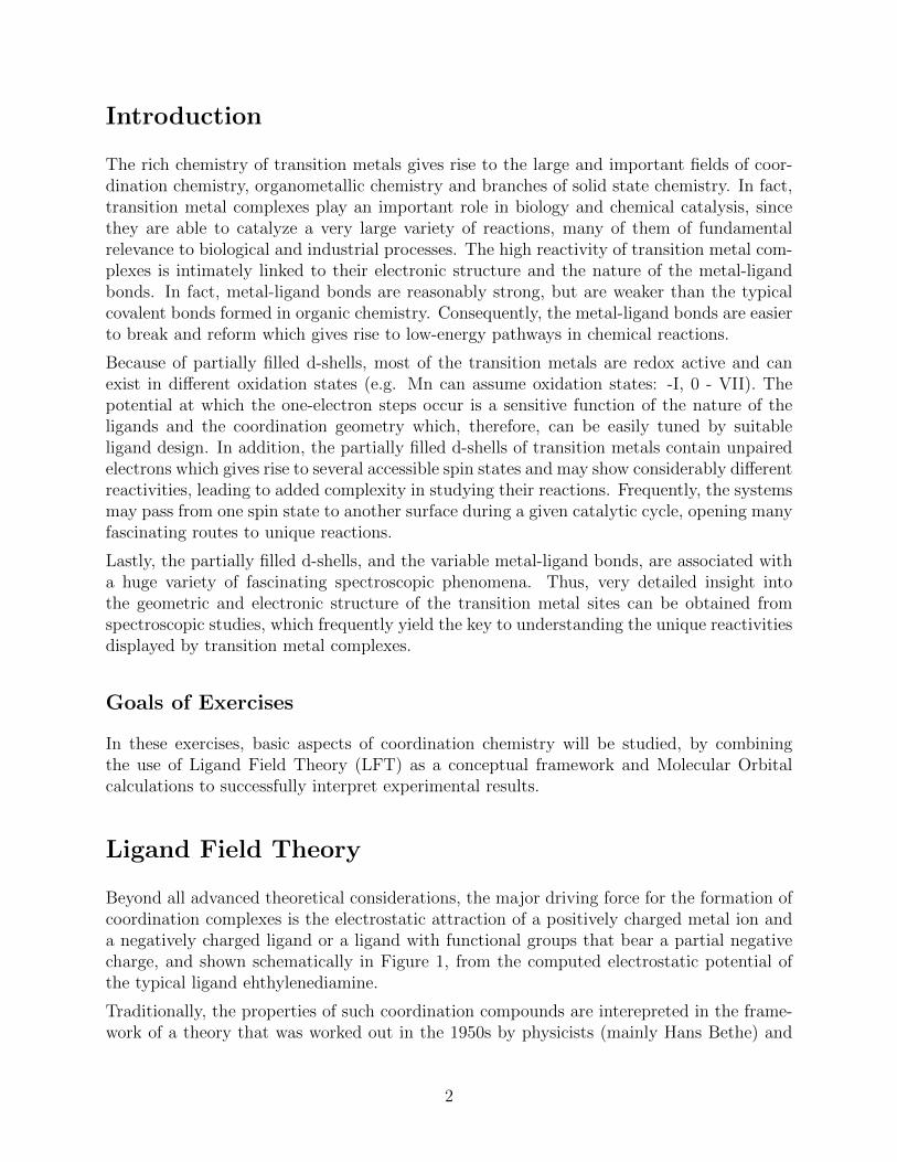
Beyond all advanced theoretical considerations, the major driving force for the formation ofcoordination complexes is the electrostatic attraction of a positively charged metal ion anda negatively charged ligand or a ligand with functional groups that bear a partial negativecharge, and shown schematically in Figure 1, from the computed electrostatic potential ofthe typical ligand ehthylenediamine.

Traditionally, the properties of such coordination compounds are interepreted in the frame-work of a theory that was worked out in the 1950s by physicists (mainly Hans Bethe) and

2

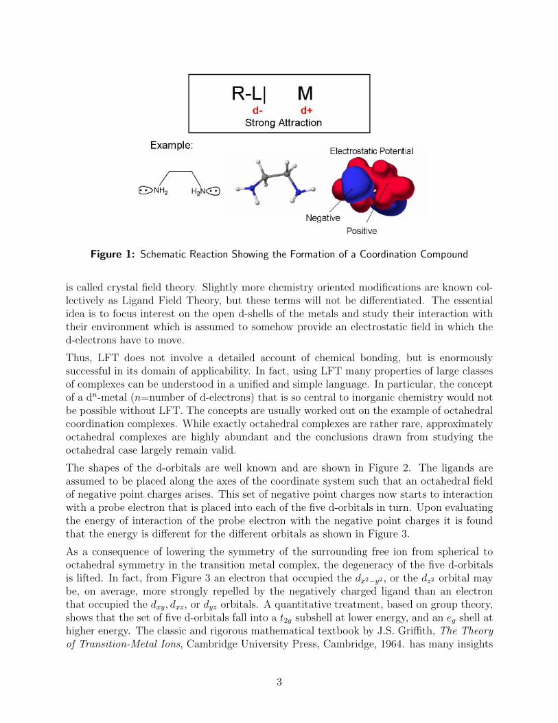
Figure 1: Schematic Reaction Showing the Formation of a Coordination Compound

is called crystal field theory. Slightly more chemistry oriented modifications are known col-lectively as Ligand Field Theory, but these terms will not be differentiated. The essentialidea is to focus interest on the open d-shells of the metals and study their interaction withtheir environment which is assumed to somehow provide an electrostatic field in which thed-electrons have to move.

Thus, LFT does not involve a detailed account of chemical bonding, but is enormouslysuccessful in its domain of applicability. In fact, using LFT many properties of large classesof complexes can be understood in a unified and simple language. In particular, the conceptof a dn-metal (n=number of d-electrons) that is so central to inorganic chemistry would notbe possible without LFT. The concepts are usually worked out on the example of octahedralcoordination complexes. While exactly octahedral complexes are rather rare, approximatelyoctahedral complexes are highly abundant and the conclusions drawn from studying theoctahedral case largely remain valid.

The shapes of the d-orbitals are well known and are shown in Figure 2. The ligands areassumed to be placed along the axes of the coordinate system such that an octahedral fieldof negative point charges arises. This set of negative point charges now starts to interactionwith a probe electron that is placed into each of the five d-orbitals in turn. Upon evaluatingthe energy of interaction of the probe electron with the negative point charges it is foundthat the energy is different for the different orbitals as shown in Figure 3.

As a consequence of lowering the symmetry of the surrounding free ion from spherical tooctahedral symmetry in the transition metal complex, the degeneracy of the five d-orbitalsis lifted. In fact, from Figure 3 an electron that occupied the dx2−y2 , or the dz2 orbital maybe, on average, more strongly repelled by the negatively charged ligand than an electronthat occupied the dxy, dxz, or dyz orbitals. A quantitative treatment, based on group theory,shows that the set of five d-orbitals fall into a t2g subshell at lower energy, and an eg shell athigher energy. The classic and rigorous mathematical textbook by J.S. Griffith, The Theoryof Transition-Metal Ions, Cambridge University Press, Cambridge, 1964. has many insights

3

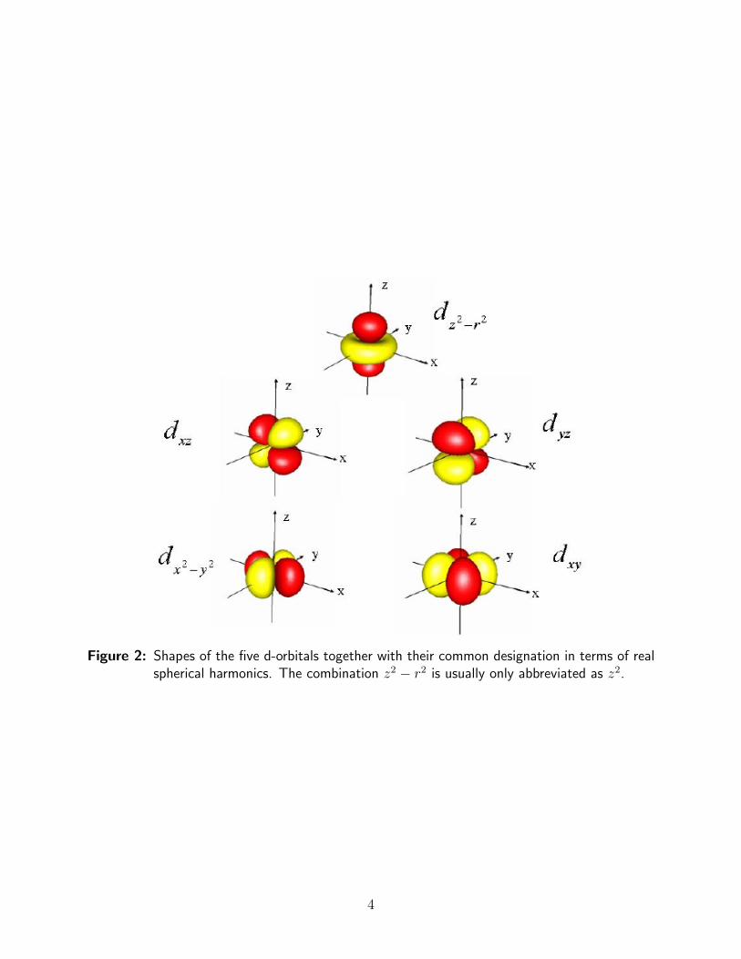
Figure 2: Shapes of the five d-orbitals together with their common designation in terms of realspherical harmonics. The combination z2 − r2 is usually only abbreviated as z2.

4

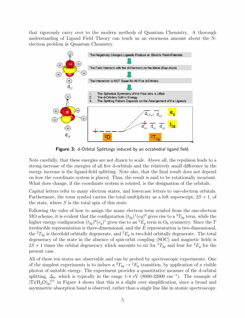
that rigorously carry over to the modern methods of Quantum Chemistry. A thoroughunderstanding of Ligand Field Theory can teach us an enormous amount about the N-electron problem in Quantum Chemistry.

Figure 3: d-Orbital Splittings induced by an octahedral ligand field.

Note carefully, that these energies are not drawn to scale. Above all, the repulsion leads to astrong increase of the energies of all five d-orbitals and the relatively small difference in theenergy increase is the ligand-field splitting. Note also, that the final result does not dependon how the coordinate system is placed. Thus, the result is said to be rotationally invariant.What does change, if the coordinate system is rotated, is the designation of the orbitals.

Capital letters refer to many electron states, and lowercase letters to one-electron orbitals.Furthermore, the term symbol carries the total multiplicity as a left superscript, 2S + 1, ofthe state, where S is the total spin of this state.

Following the rules of how to assign the many electron term symbol from the one-electronMO scheme, it is evident that the configuration (t2g)

1(eg)0 gives rise to a 2T2g term, while thehigher energy configuration (t2g)

0(eg)1 gives rise to an 2Eg term in Oh symmetry. Since the T

irreducible representation is three-dimensional, and the E representation is two-dimensional,the 2T2g is threefold orbitally degenerate, and 2Eg is two-fold orbitally degenerate. The totaldegeneracy of the state in the absence of spin-orbit coupling (SOC) and magnetic fields is2S + 1 times the orbital degeneracy which amounts to six for 2T2g and four for 2Eg for thepresent case.

All of these ten states are observable and can be probed by spectroscopic experiments. Oneof the simplest experiments is to induce a 2T2g → 2Eg transition, by application of a visiblephoton of suitable energy. The experiment provides a quantitative measure of the d-orbitalsplitting, ∆0, which is typically in the range 1-4 eV (8000-32000 cm−1). The example of[Ti(H2O)6]

3+ in Figure 4 shows that this is a slight over simplification, since a broad andasymmetric absorption band is observed, rather than a single line like in atomic spectroscopy.

5

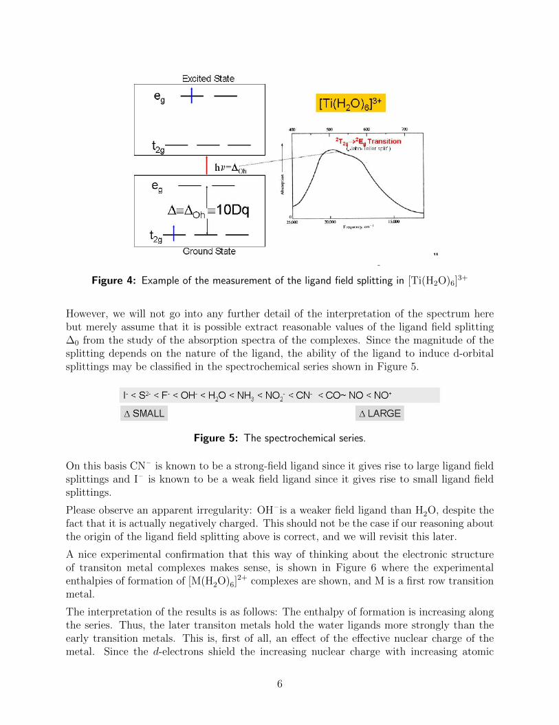
Figure 4: Example of the measurement of the ligand field splitting in [Ti(H2O)6]3+

However, we will not go into any further detail of the interpretation of the spectrum herebut merely assume that it is possible extract reasonable values of the ligand field splitting∆0 from the study of the absorption spectra of the complexes. Since the magnitude of thesplitting depends on the nature of the ligand, the ability of the ligand to induce d-orbitalsplittings may be classified in the spectrochemical series shown in Figure 5.

Figure 5: The spectrochemical series.

On this basis CN– is known to be a strong-field ligand since it gives rise to large ligand fieldsplittings and I– is known to be a weak field ligand since it gives rise to small ligand fieldsplittings.

Please observe an apparent irregularity: OH– is a weaker field ligand than H2O, despite thefact that it is actually negatively charged. This should not be the case if our reasoning aboutthe origin of the ligand field splitting above is correct, and we will revisit this later.

A nice experimental confirmation that this way of thinking about the electronic structureof transiton metal complexes makes sense, is shown in Figure 6 where the experimentalenthalpies of formation of [M(H2O)6]

2+ complexes are shown, and M is a first row transitionmetal.

The interpretation of the results is as follows: The enthalpy of formation is increasing alongthe series. Thus, the later transiton metals hold the water ligands more strongly than theearly transition metals. This is, first of all, an effect of the effective nuclear charge of themetal. Since the d-electrons shield the increasing nuclear charge with increasing atomic

6

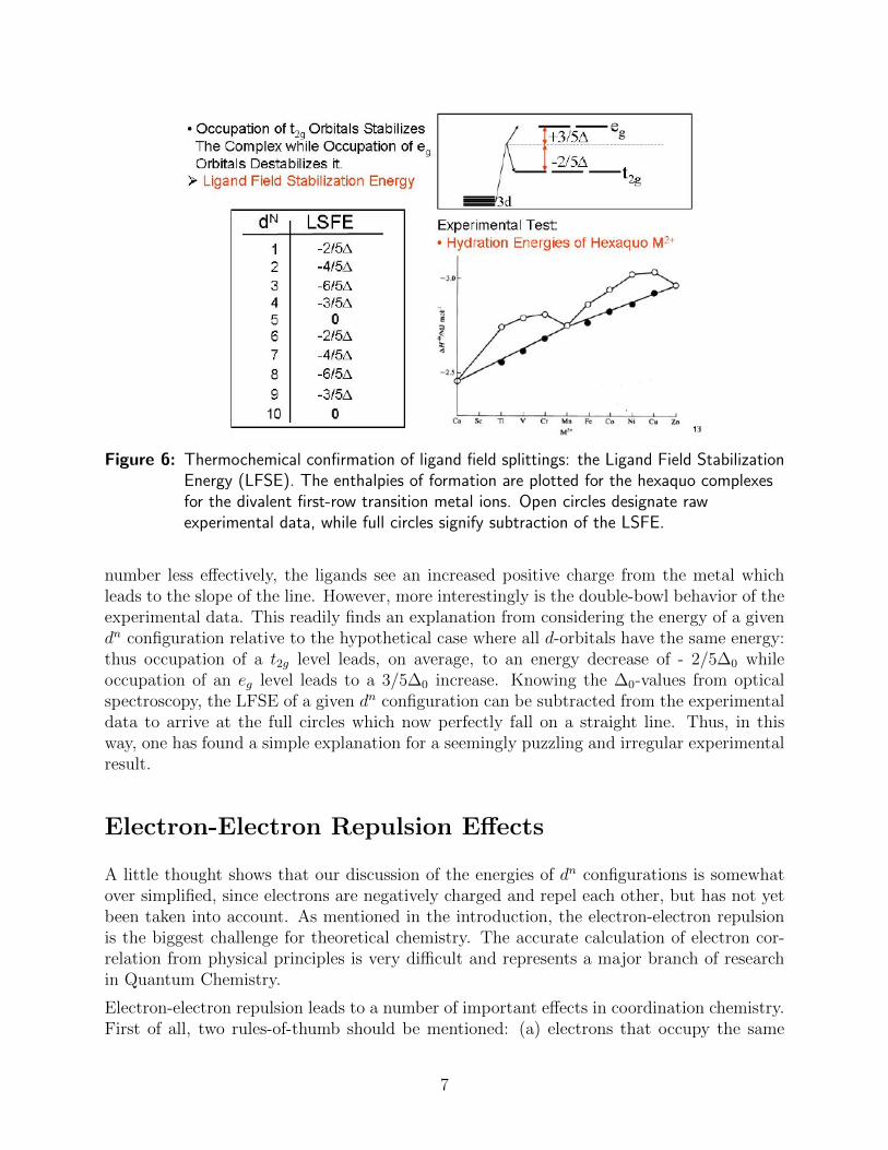
Figure 6: Thermochemical confirmation of ligand field splittings: the Ligand Field StabilizationEnergy (LFSE). The enthalpies of formation are plotted for the hexaquo complexesfor the divalent first-row transition metal ions. Open circles designate rawexperimental data, while full circles signify subtraction of the LSFE.

number less effectively, the ligands see an increased positive charge from the metal whichleads to the slope of the line. However, more interestingly is the double-bowl behavior of theexperimental data. This readily finds an explanation from considering the energy of a givendn configuration relative to the hypothetical case where all d-orbitals have the same energy:thus occupation of a t2g level leads, on average, to an energy decrease of - 2/5∆0 whileoccupation of an eg level leads to a 3/5∆0 increase. Knowing the ∆0-values from opticalspectroscopy, the LFSE of a given dn configuration can be subtracted from the experimentaldata to arrive at the full circles which now perfectly fall on a straight line. Thus, in thisway, one has found a simple explanation for a seemingly puzzling and irregular experimentalresult.

Electron-Electron Repulsion Effects

A little thought shows that our discussion of the energies of dn configurations is somewhatover simplified, since electrons are negatively charged and repel each other, but has not yetbeen taken into account. As mentioned in the introduction, the electron-electron repulsionis the biggest challenge for theoretical chemistry. The accurate calculation of electron cor-relation from physical principles is very difficult and represents a major branch of researchin Quantum Chemistry.

Electron-electron repulsion leads to a number of important effects in coordination chemistry.First of all, two rules-of-thumb should be mentioned: (a) electrons that occupy the same

7

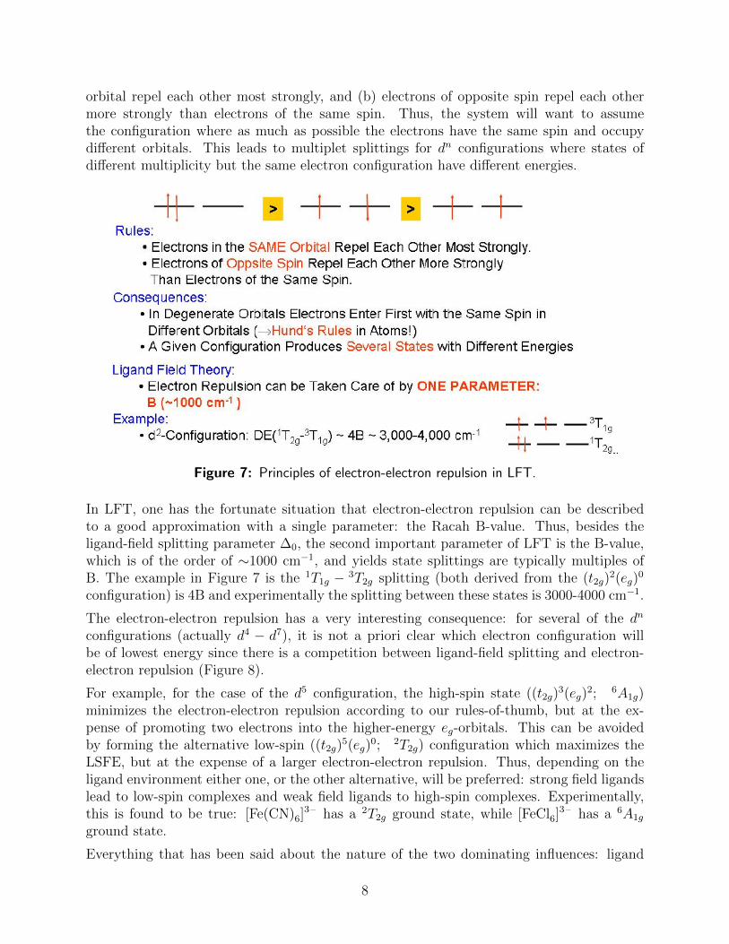
orbital repel each other most strongly, and (b) electrons of opposite spin repel each othermore strongly than electrons of the same spin. Thus, the system will want to assumethe configuration where as much as possible the electrons have the same spin and occupydifferent orbitals. This leads to multiplet splittings for dn configurations where states ofdifferent multiplicity but the same electron configuration have different energies.

Figure 7: Principles of electron-electron repulsion in LFT.

In LFT, one has the fortunate situation that electron-electron repulsion can be describedto a good approximation with a single parameter: the Racah B-value. Thus, besides theligand-field splitting parameter ∆0, the second important parameter of LFT is the B-value,which is of the order of ∼1000 cm−1, and yields state splittings are typically multiples ofB. The example in Figure 7 is the 1T1g − 3T2g splitting (both derived from the (t2g)

2(eg)0

configuration) is 4B and experimentally the splitting between these states is 3000-4000 cm−1.

The electron-electron repulsion has a very interesting consequence: for several of the dn

configurations (actually d4 − d7), it is not a priori clear which electron configuration willbe of lowest energy since there is a competition between ligand-field splitting and electron-electron repulsion (Figure 8).

For example, for the case of the d5 configuration, the high-spin state ((t2g)3(eg)

2; 6A1g)minimizes the electron-electron repulsion according to our rules-of-thumb, but at the ex-pense of promoting two electrons into the higher-energy eg-orbitals. This can be avoidedby forming the alternative low-spin ((t2g)

5(eg)0; 2T2g) configuration which maximizes the

LSFE, but at the expense of a larger electron-electron repulsion. Thus, depending on theligand environment either one, or the other alternative, will be preferred: strong field ligandslead to low-spin complexes and weak field ligands to high-spin complexes. Experimentally,this is found to be true: [Fe(CN)6]

3– has a 2T2g ground state, while [FeCl6]3– has a 6A1g

ground state.

Everything that has been said about the nature of the two dominating influences: ligand

8

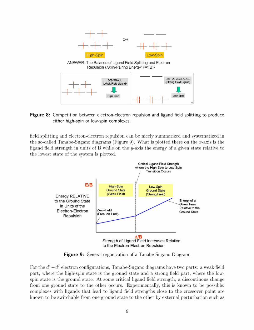
Figure 8: Competition between electron-electron repulsion and ligand field splitting to produceeither high-spin or low-spin complexes.

field splitting and electron-electron repulsion can be nicely summarized and systematized inthe so-called Tanabe-Sugano diagrams (Figure 9). What is plotted there on the x-axis is theligand field strength in units of B while on the y-axis the energy of a given state relative tothe lowest state of the system is plotted.

Figure 9: General organization of a Tanabe-Sugano Diagram.

For the d4−d7 electron configurations, Tanabe-Sugano diagrams have two parts: a weak fieldpart, where the high-spin state is the ground state and a strong field part, where the low-spin state is the ground state. At some critical ligand field strength, a discontinous changefrom one ground state to the other occurs. Experimentally, this is known to be possible:complexes with ligands that lead to ligand field strengths close to the crossover point areknown to be switchable from one ground state to the other by external perturbation such as

9

pressure.

This leads to the interesting field of spin-crossover chemistry which is a promising approachto the design of molecular switches. Secondly, the Tanabe-Sugano diagrams are excellentguides to the assignment of the ligand-field absorption spectra of transiton metal complexes.Given that the selection rule, S = 0, for an electric dipole allowed transition between twostates is fairly strong, one simply has to search in the Tanabe-Sugano diagram for states ofthe same multiplicity as the ground state in order to find out how many ligand-field bandsare expected in the absorption spectrum.

The only thing that is needed, then, in order to determine ∆0, is a ruler and a reasonableestimate of B. Two examples of such diagrams together with actual absorption spectra areshown in Figure 10.

The spin-allowed ligand field bands are weak, since they are parity forbidden in octahedralcomplexes. However, in tetrahedral complexes, there is no center of inversion, and theobserved ligand field bands are much stronger than in octahedral complexes. Spin-allowedligand field bands can have absorbtivity (ε) values that are several hundred M−1cm−1, whilespin-forbidden transitions typically have absorbtivity (ε) values < 1 M−1cm−1.

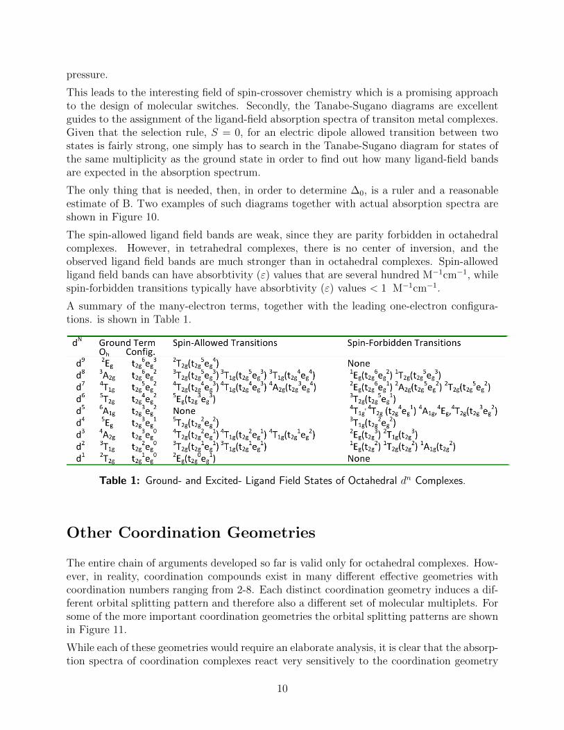
A summary of the many-electron terms, together with the leading one-electron configura-tions. is shown in Table 1.

Table 1: Ground- and Excited- Ligand Field States of Octahedral dn Complexes.

Other Coordination Geometries

The entire chain of arguments developed so far is valid only for octahedral complexes. How-ever, in reality, coordination compounds exist in many different effective geometries withcoordination numbers ranging from 2-8. Each distinct coordination geometry induces a dif-ferent orbital splitting pattern and therefore also a different set of molecular multiplets. Forsome of the more important coordination geometries the orbital splitting patterns are shownin Figure 11.

While each of these geometries would require an elaborate analysis, it is clear that the absorp-tion spectra of coordination complexes react very sensitively to the coordination geometry

10

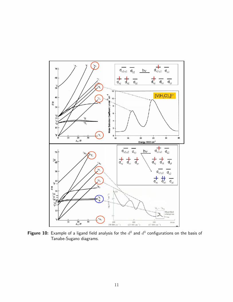
Figure 10: Example of a ligand field analysis for the d2 and d3 configurations on the basis ofTanabe-Sugano diagrams.

11

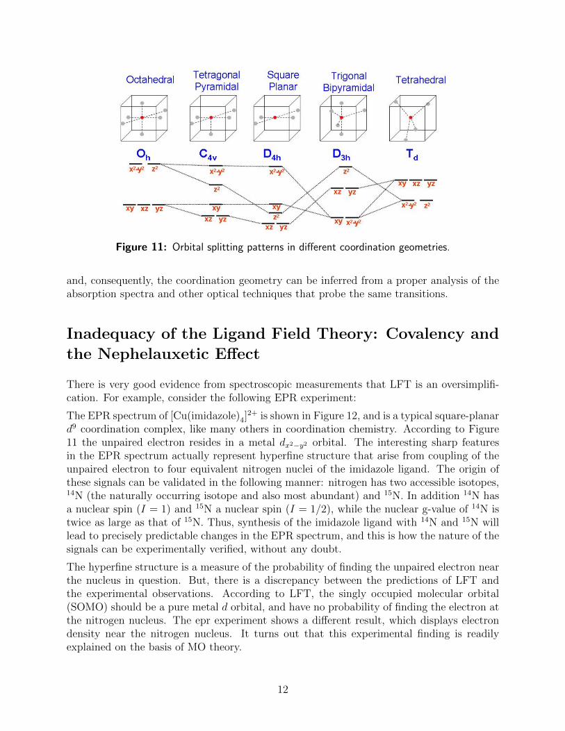
Figure 11: Orbital splitting patterns in different coordination geometries.

and, consequently, the coordination geometry can be inferred from a proper analysis of theabsorption spectra and other optical techniques that probe the same transitions.

Inadequacy of the Ligand Field Theory: Covalency and

the Nephelauxetic Effect

There is very good evidence from spectroscopic measurements that LFT is an oversimplifi-cation. For example, consider the following EPR experiment:

The EPR spectrum of [Cu(imidazole)4]2+ is shown in Figure 12, and is a typical square-planar

d9 coordination complex, like many others in coordination chemistry. According to Figure11 the unpaired electron resides in a metal dx2−y2 orbital. The interesting sharp featuresin the EPR spectrum actually represent hyperfine structure that arise from coupling of theunpaired electron to four equivalent nitrogen nuclei of the imidazole ligand. The origin ofthese signals can be validated in the following manner: nitrogen has two accessible isotopes,14N (the naturally occurring isotope and also most abundant) and 15N. In addition 14N hasa nuclear spin (I = 1) and 15N a nuclear spin (I = 1/2), while the nuclear g-value of 14N istwice as large as that of 15N. Thus, synthesis of the imidazole ligand with 14N and 15N willlead to precisely predictable changes in the EPR spectrum, and this is how the nature of thesignals can be experimentally verified, without any doubt.

The hyperfine structure is a measure of the probability of finding the unpaired electron nearthe nucleus in question. But, there is a discrepancy between the predictions of LFT andthe experimental observations. According to LFT, the singly occupied molecular orbital(SOMO) should be a pure metal d orbital, and have no probability of finding the electron atthe nitrogen nucleus. The epr experiment shows a different result, which displays electrondensity near the nitrogen nucleus. It turns out that this experimental finding is readilyexplained on the basis of MO theory.

12

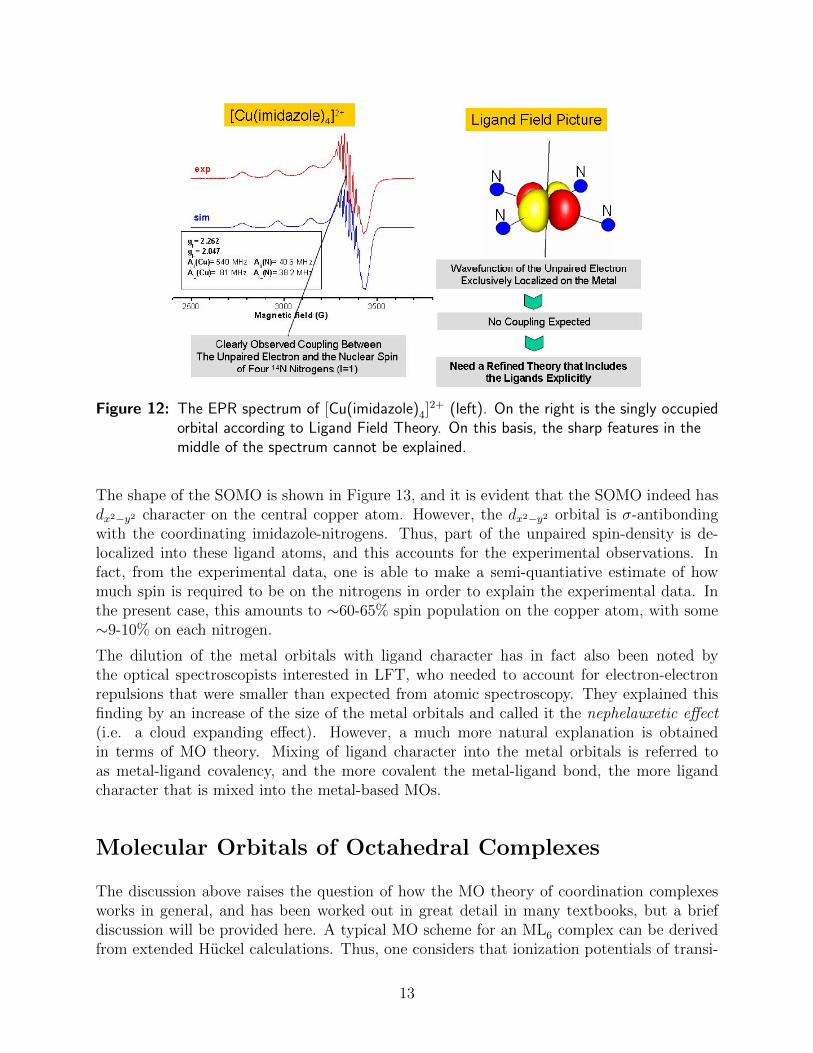
Figure 12: The EPR spectrum of [Cu(imidazole)4]2+ (left). On the right is the singly occupied

orbital according to Ligand Field Theory. On this basis, the sharp features in themiddle of the spectrum cannot be explained.

The shape of the SOMO is shown in Figure 13, and it is evident that the SOMO indeed hasdx2−y2 character on the central copper atom. However, the dx2−y2 orbital is σ-antibondingwith the coordinating imidazole-nitrogens. Thus, part of the unpaired spin-density is de-localized into these ligand atoms, and this accounts for the experimental observations. Infact, from the experimental data, one is able to make a semi-quantiative estimate of howmuch spin is required to be on the nitrogens in order to explain the experimental data. Inthe present case, this amounts to ∼60-65% spin population on the copper atom, with some∼9-10% on each nitrogen.

The dilution of the metal orbitals with ligand character has in fact also been noted bythe optical spectroscopists interested in LFT, who needed to account for electron-electronrepulsions that were smaller than expected from atomic spectroscopy. They explained thisfinding by an increase of the size of the metal orbitals and called it the nephelauxetic effect(i.e. a cloud expanding effect). However, a much more natural explanation is obtainedin terms of MO theory. Mixing of ligand character into the metal orbitals is referred toas metal-ligand covalency, and the more covalent the metal-ligand bond, the more ligandcharacter that is mixed into the metal-based MOs.

Molecular Orbitals of Octahedral Complexes

The discussion above raises the question of how the MO theory of coordination complexesworks in general, and has been worked out in great detail in many textbooks, but a briefdiscussion will be provided here. A typical MO scheme for an ML6 complex can be derivedfrom extended Huckel calculations. Thus, one considers that ionization potentials of transi-

13

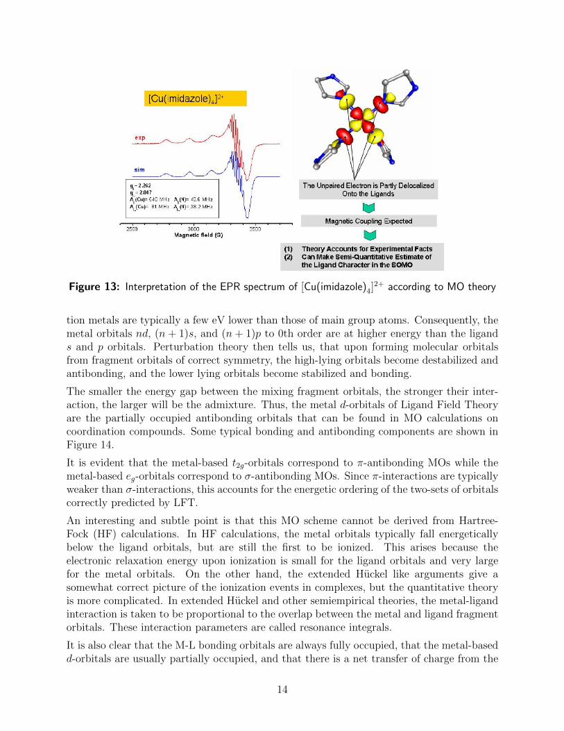
Figure 13: Interpretation of the EPR spectrum of [Cu(imidazole)4]2+ according to MO theory

tion metals are typically a few eV lower than those of main group atoms. Consequently, themetal orbitals nd, (n + 1)s, and (n + 1)p to 0th order are at higher energy than the ligands and p orbitals. Perturbation theory then tells us, that upon forming molecular orbitalsfrom fragment orbitals of correct symmetry, the high-lying orbitals become destabilized andantibonding, and the lower lying orbitals become stabilized and bonding.

The smaller the energy gap between the mixing fragment orbitals, the stronger their inter-action, the larger will be the admixture. Thus, the metal d-orbitals of Ligand Field Theoryare the partially occupied antibonding orbitals that can be found in MO calculations oncoordination compounds. Some typical bonding and antibonding components are shown inFigure 14.

It is evident that the metal-based t2g-orbitals correspond to π-antibonding MOs while themetal-based eg-orbitals correspond to σ-antibonding MOs. Since π-interactions are typicallyweaker than σ-interactions, this accounts for the energetic ordering of the two-sets of orbitalscorrectly predicted by LFT.

An interesting and subtle point is that this MO scheme cannot be derived from Hartree-Fock (HF) calculations. In HF calculations, the metal orbitals typically fall energeticallybelow the ligand orbitals, but are still the first to be ionized. This arises because theelectronic relaxation energy upon ionization is small for the ligand orbitals and very largefor the metal orbitals. On the other hand, the extended Huckel like arguments give asomewhat correct picture of the ionization events in complexes, but the quantitative theoryis more complicated. In extended Huckel and other semiempirical theories, the metal-ligandinteraction is taken to be proportional to the overlap between the metal and ligand fragmentorbitals. These interaction parameters are called resonance integrals.

It is also clear that the M-L bonding orbitals are always fully occupied, that the metal-basedd-orbitals are usually partially occupied, and that there is a net transfer of charge from the

14

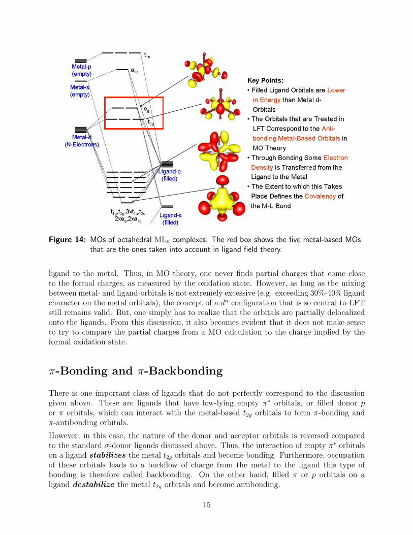
Figure 14: MOs of octahedral ML6 complexes. The red box shows the five metal-based MOsthat are the ones taken into account in ligand field theory.

ligand to the metal. Thus, in MO theory, one never finds partial charges that come closeto the formal charges, as measured by the oxidation state. However, as long as the mixingbetween metal- and ligand-orbitals is not extremely excessive (e.g. exceeding 30%-40% ligandcharacter on the metal orbitals), the concept of a dn configuration that is so central to LFTstill remains valid. But, one simply has to realize that the orbitals are partially delocalizedonto the ligands. From this discussion, it also becomes evident that it does not make senseto try to compare the partial charges from a MO calculation to the charge implied by theformal oxidation state.

π-Bonding and π-Backbonding

There is one important class of ligands that do not perfectly correspond to the discussiongiven above. These are ligands that have low-lying empty π∗ orbitals, or filled donor por π orbitals, which can interact with the metal-based t2g orbitals to form π-bonding andπ-antibonding orbitals.

However, in this case, the nature of the donor and acceptor orbitals is reversed comparedto the standard σ-donor ligands discussed above. Thus, the interaction of empty π∗ orbitalson a ligand stabilizes the metal t2g orbitals and become bonding. Furthermore, occupationof these orbitals leads to a backflow of charge from the metal to the ligand this type ofbonding is therefore called backbonding. On the other hand, filled π or p orbitals on aligand destabilize the metal t2g orbitals and become antibonding.

15

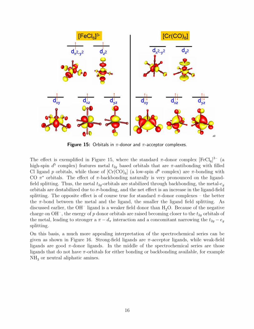
Figure 15: Orbitals in π-donor and π-acceptor complexes.

The effect is exemplified in Figure 15, where the standard π-donor complex [FeCl6]3– (a

high-spin d5 complex) features metal t2g based orbitals that are π-antibonding with filledCl ligand p orbitals, while those of [Cr(CO)6] (a low-spin d6 complex) are π-bonding withCO π∗ orbitals. The effect of π-backbonding naturally is very pronounced on the ligand-field splitting. Thus, the metal t2g-orbitals are stabilized through backbonding, the metal-egorbitals are destabilized due to σ-bonding, and the net effect is an increase in the ligand-fieldsplitting. The opposite effect is of course true for standard π-donor complexes – the betterthe π-bond between the metal and the ligand, the smaller the ligand field splitting. Asdiscussed earlier, the OH– ligand is a weaker field donor than H2O. Because of the negativecharge on OH– , the energy of p donor orbitals are raised becoming closer to the t2g orbitals ofthe metal, leading to stronger a π− dπ interaction and a concomitant narrowing the t2g − egsplitting.

On this basis, a much more appealing interpretation of the spectrochemical series can begiven as shown in Figure 16. Strong-field ligands are π-acceptor ligands, while weak-fieldligands are good π-donor ligands. In the middle of the spectrochemical series are thoseligands that do not have π-orbitals for either bonding or backbonding available, for exampleNH3 or neutral aliphatic amines.

16

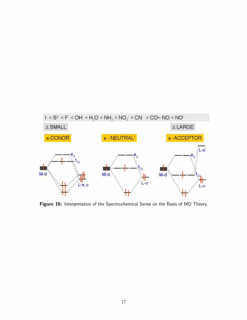
Figure 16: Interpretation of the Spectrochemical Series on the Basis of MO Theory.

17

General Comments for the Calculations

Below are several problems in computational coordination chemistry that are more or lessrepresentative of transition metal coordination chemistry.

In general very small basis sets (SV for the metal and the oxygens and STO-3G for thehydrogens) will be used in order to minimize calculation times. In practice, it is advisable touse at least polarized triple-ζ basis sets for the metals and at least polarized double-ζ basissets for the ligands in order to obtain reliable results.

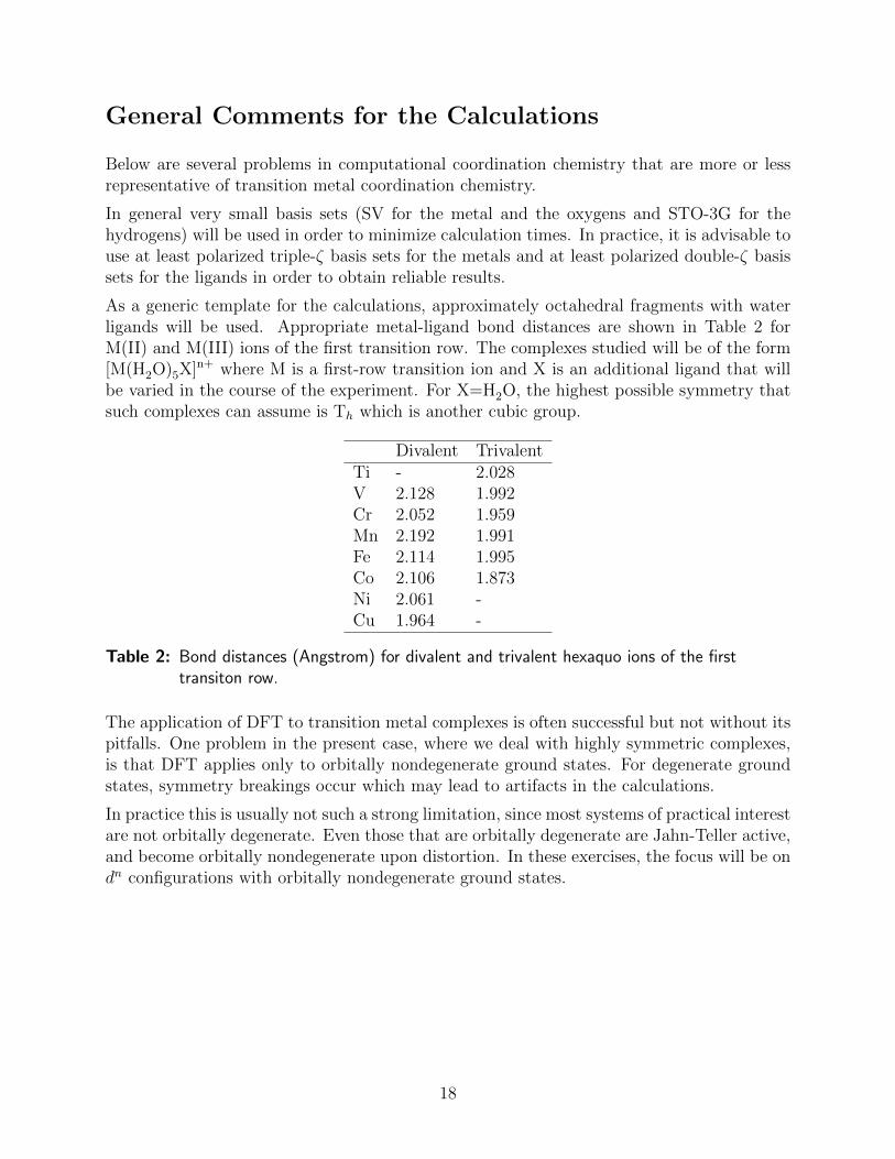
As a generic template for the calculations, approximately octahedral fragments with waterligands will be used. Appropriate metal-ligand bond distances are shown in Table 2 forM(II) and M(III) ions of the first transition row. The complexes studied will be of the form[M(H2O)5X]n+ where M is a first-row transition ion and X is an additional ligand that willbe varied in the course of the experiment. For X=H2O, the highest possible symmetry thatsuch complexes can assume is Th which is another cubic group.

Divalent TrivalentTi - 2.028V 2.128 1.992Cr 2.052 1.959Mn 2.192 1.991Fe 2.114 1.995Co 2.106 1.873Ni 2.061 -Cu 1.964 -

Table 2: Bond distances (Angstrom) for divalent and trivalent hexaquo ions of the firsttransiton row.

The application of DFT to transition metal complexes is often successful but not without itspitfalls. One problem in the present case, where we deal with highly symmetric complexes,is that DFT applies only to orbitally nondegenerate ground states. For degenerate groundstates, symmetry breakings occur which may lead to artifacts in the calculations.

In practice this is usually not such a strong limitation, since most systems of practical interestare not orbitally degenerate. Even those that are orbitally degenerate are Jahn-Teller active,and become orbitally nondegenerate upon distortion. In these exercises, the focus will be ondn configurations with orbitally nondegenerate ground states.

18

Intersection of Ligand Field Theory and Density Functional Theory

1. Perform calculations for the [Cr(H2O)6]3+ complex, and on other similar d3 complexes,

including [V(H2O)6]2+, the hypothetical [Ti(H2O)6]

+, the d8 system, [Ni(H2O)]2+, andhypothetical [Cu(H2O)6]

3+.

Observe the results of the population analysis. How does the partial charge on themetal change? How does the spin-population at the metal change?

Look at the occupancies of the metal d-orbitals. What does that say about σ− andπ−donation of the water ligands? How does it compare with the formal occupations?Compare the spin-populations of the d3 and d8 systems. What do you observe?

2. Calculate the first six ligand field excited states for the transition metal complexesgiven in Question 1 above, and determine ∆0 and B from the computational results.

The energies of the two transitions from LFT for both the d3 and d8 complexes, aregiven by:

d3 d8 Energy4A2g → 4T2g

3A2g → 3T2g ∆E = ∆04A2g → 4T1g

3A2g → 3T1g ∆E = ∆0 + 12 B

Thus, from the calculations, the values of 0 and B can easily be determined.

3. The ratio ofB(complex)B(free ion)

is known as the nephelauxetic ratio. Calculate the nephelaux-

etic ratios for the series of complexes given in Question 1 above.

The Racah-parameters (B) of the free ions are: Cr3+=950 cm−1, Ti2+=720 cm−1,Ti+=680 cm−1, V2+=765 cm−1, V3+=860 cm−1, Ni2+=1080 cm−1, Ni+=1040 cm−1 ,Cu2+=1240 cm−1, Cu+=1220 cm−1, Cu3+=1260 cm−1.

Are the nephelauxetic ratios larger or smaller than unity? Explain. Do the trends innephelauxetic ratios make sense in terms of your chemical intuition?

Will the nephelauxetic ratios depend on the nature of the metal, including the oxidationstate and the ligand? Please explain your answer.

What do you include with respect to the ability of TD-DFT to model the values ∆0

and B correctly?

4. Study the dependence of ∆0 and B on the metal-ligand distance of [Cr(H2O)6]3+. Does

the result match your expectation?

Which power of the metal-ligand distance R do you expect ∆0 to vary based on con-ventional ligand field arguments?

Positions of Ligand and d Orbitals in Transition Metal complexes

In many cases, it is difficult to unambiguously identify the metal based MOs. This is par-ticularly so for later metals, higher oxidation states, and increasing numbers of unpaired

19

electrons. The reason is that higher oxidation states tend to stabilize the d-orbitals, and,consequently, move closer to the ligand orbitals. In addition, a large number of singly occu-pied orbitals that are mainly centered on the metal lead to a very large exchange stabilizationwhich further suppresses the energies of the occupied spin-up orbitals.

As a consequence, metal-based MOs move down in energy near or below the ligand basedorbitals. This effect is more pronounced as more Hartree-Fock exchange is present in thedensity functional, and is extremely strong for the Hartree-Fock method itself. Yet, theligand field picture is not invalid but simply more difficult to recover from MO calculations.

One useful way to unravel the distinction between ligand and d orbital involves a localizationprocedure, followed by analysis and visualization of the localized orbitals (LCOs) composedof mainly metal character.

Localized orbitals never show a bond where there is none. Thus, if a bonding and anantibonding partner of a bond are both fully occupied, the localization procedure simplyseparates the two constituents into atomic or fragment orbitals. A bond remains only if theantibonding partner is in the virtual space. Thus, localization and orbital inspection is agood way to discuss the net bonding effects.

Another useful way to obtain a clearer discription of ligand and d orbital is through the cal-culation of Restricted Orbitals (QROs), where those that are singly occupied will correspondwell with ligand field expectations and is another useful analysis tool.

1. Perform a calculation on [Fe(H2O)6]3+ and inspect the canonical orbitals in both the

spin-up and spin-down sets. Where are the metal orbitals? What is their composition?What are their energies? How would you interpret these results?

2. Localize the orbitals, and then visualize them.

What does your result imply in terms of frontier molecular orbital theory? Where doyou think will an electron go upon reduction of the complex to the ferrous form?

3. Obtain a set of QROs, and analyze their composition, and visualize them.

Do these results with QROs lead to a better description for the ligand and d orbitals?

Covalencies of Metal Ligand Bonds

As mentioned in the introduction to this chapter, the coalvency of the metal ligand bonds isan important factor in determining the physical and reactive properties of transition metalcomplexes. Covalency here is defined as the ability of the metal and the ligand to shareelectrons. A quantitative measure for this is how much ligand character is mixed into themetal d-based orbitals, and vice versa.

The unitary invariance of the wavefunction (or Kohn-Sham determinant) with respect torotations among occupied orbitals are not observables. However, it is chemically sensibleto study the variations in metal-ligand bonding by looking at the metal-ligand bonding andantibonding orbitals.

20

Consider the [M(H2O)6(X)]n+ complexes and vary X for fixed M and then M for fixed X,where X can be: CO, CN– , NH3, OH2, O2– , S2– , F– , Cl– , Br– , and I– .

1. For the hypothetical complexes [Cr(H2O)5(X)]3+, [Cr(H2O)5(X– )]2+, and [Cr(H2O)5(X

2– )]+,optimize the geometry of the complexes using the small basis set defined above.

Calculate the energies of the system using the B3LYP functional in single point cal-culations, and include a water solvation model. Look at the metal-t2g and metal-egderived orbitals.

Discuss σ-bonding versus π-backbonding, and how it varies with the ligand. Whatchanges are observed in the populations of the metal d-orbitals?

2. Analyze and visualize localized molecular orbitals.

Localized orbitals never show a bond where there is none. Thus, if a bonding andan antibonding partner of a bond are both fully occupied, the localization proceduresimply separates the two constituents into atomic or fragment orbitals. A bond remainsonly if the antibonding partner is in the virtual space. Thus, localization and orbitalinspection is a good way to discuss the net bonding effects.

What conclusions can be inferred about the nature of the bonds?

3. From the total energy calculations, compare the bond energy of the X ligand relativeto the hexaquo complex. It will be necessary to run a geometry optimization plusenergy for the free X ligands. How does the bond energy vary with the ligand and theoxidation state of the metal? Is it in accord with your chemical intuition?

4. Repeat the calculations for fixed ligands with a lower-valent metal, for example, thelow-spin configuration (S = 0) of Fe(II). How does the ability of the metal for back-bonding change?

Organometallics

The field or organometallic chemistry is quite important because versatile and powerfulcatalysts can be designed on the basis of such complexes. Here, a brief look is taken at aniconic organometallic compound, ferrocene, Fe(cp)2.

1. Run a single point calculation on Fe(cp)2 using the BP86 functional and the smallbasis set used throughout these exercises.

Analyze the electronic structure of the complex using orbitals and populations. Whatis the nature of the metal ligand bond?

2. Perform a calculation on the free cyclopentadienyl ligand and determine the fragmentorbitals that contribute most to the bonding. Construct a fragment orbital interactiondiagram.

21

3. Use the BHLYP functional to calculate the first 15 electronically excited states.

What is the nature of these transitions, and compare the transition energies with d−dtransition energies of the hexaquo complexes that were studied above. What do youobserve? What is the interpretation of what is observed? Determine the dominantdonor and acceptor orbital pairs. Work out the symmetry of the final electronic states.Determine the selection rules for the electric dipole and magnetic dipole transitions.

Potential Energy Scan of [CuCl4]2−

The complex ion [CuCl4]2– is known to exist in different crystals with varying counterions.

While Cu(II) normally prefers a square planar coordination, this ion is found in variousforms ranging from square-planar to almost tetrahedral.

The energy associated with this distortion will be calculated. A rigid potential energy surface,beginning with a square planar and ending with a tetrahedral structure, is performed bydefining a Cl-Cu-Cl distortion angle which varies from 0 to a final value of (180-109.4712)/2.

1. Perform the potential energy scan, convert the energies to relative energies in kcal/mol,and plot the resulting potential energy surface.

A larger number of steps can be employed in order to obtain a more smooth lookingsurface.

Where do you find the minimum? Does it require a lot of energy to distort the molecule?

2. Determine the change in electronic structure by examining two or three points alongthe surface.

Examine the orbitals and populations.

3. Calculate the first four ligand field excited states. Do you think that spectroscopy willbe a useful indicator of the coordination geometry?

This calculation represents one of the cases where TD-DFT with normal GGA func-tionals like BP86 fails badly, and predicts LMCT states where there should be d-dexcitations (in the region below ∼15000 cm−1). The calculation should, instead, beperformed with a functional that includes more HF exchange. BHLYP is recommendedwhich introduces as much as 50% HF exchange. It may also be necessary to calculatemore than the desired four ligand field states in order to capture the states of interest,since they do not come in order of increasing orbital energy difference. To be on thesafe side, a calculation with 25 states should be sufficient. Observe the assignment ofthe transitions and see where the occupied metal orbitals are in the spin down set.

Draw an MO diagram.

Reactivity: Powerful Oxidants

The interesting species [Fe(IV)O(H2O)5]2+ has been synthesized and will be studied in sec-

tion. It is a simple model for related Fe(IV)-oxo species that are of much relevance to

22

chemistry and biochemistry since they are powerful oxidants. The most intensely studiedsystem is Cytochrome P450 which features a very complicated electronic structure. Theactive species involves an iron-oxo group coupled to a porphyrin radical.

Some aspects of structure, bonding and energetics of such species will be studied.

1. Firstly, determine which spin state is the lowest one for this system, i.e. S = 1 or 2.Optimize the structure of the species. Repeat the optimization for the low-spin state.

2. Analyze the electronic structure of both species.

What are the electron configurations in the two states? How did the structure change?

How did the changes in the structure reflect the different electronic configurations? Isthe oxo-group strongly affected by the change in spin state?

More interestingly for the synthetically oriented chemists is the question of how tochoose a ligand which will force the system to adopt either one or the other groundstate?

3. Recalculate the energies at the optimized geometries using the B3LYP functional.

For more quantative results, is necessary to perform the calculation with much largerbasis sets: geometry optimization with TZVP basis set, and final energy calculationwith TZVPP basis set. This will not be done here, in order to keep the computationtimes short. In a serious study, one would also want to evaluate the zero-point energyand thermal contributions to the energy differences.

What is the energy difference between the two states? Could either be the groundstate?

4. Study the hydrogen atom abstraction reaction:

[FeO(H2O)5]2+ + CH4 → [Fe(OH)(H2O)5]

2+ + CH3

• Optimize the structures of the reactants and products (assume S = 5/2).

• Recalculate the energies using B3LYP single point calculations.

• Is the reaction predicted to be feasible? If not, would this molecule be able tooxidize weaker C-H bonds such as that of toluene?

• Analyze the structure of the reaction product. What are the major geometricchanges? What are the electronic changes brought about by protonating the oxogroup and reducing the metal? What happens to the Fe−O bond and covalency?

5. Compare the capability of this iron-oxo species to two other systems: OH· radicaland the well-known species, [VO(H2O)5]

2+ which will require another set of geometryoptimizations.

23

Unusual Bonds and Coordinated Radicals: Iron-Nitrosyls

Questions of structure and bonding can become quite complicated when the oxidation stateof the ligand becomes ambiguous. A famous example are transition metal nitrosyls. Herethe NO ligand is believed to be able to coordinate as NO– (S=1), NO– (S=0), NO·(S=1/2)and NO+(S=0) depending on the metal and formal oxidation state, and the remaining ligandset. Since the interpretation is often ambiguous, Enemark and Feltham have invented the{MNO}x notation, where x is the number of metal-d plus NO-π∗ electrons. Thus, thereaction of Fe(II) with NO yields a {FeNO}7 complex.

The [Fe(H2O)5(NO)]3+ complex ion will be studied, and is well-known to every chemist as thebrown ring complex in analytic chemistry, but has a quite complicated electronic structure.

1. Optimize the geometries of [Fe(III)(H2O)5(NO+)]3+

(S = 5/2), [Fe(II)(H2O)5(NO·)]3+ (S =3/2), and [Fe(I)(H2O)5(NO−)]

3+(S = 1).

Use initial parameters with an Fe−NO bond distance of 1.76 A, Fe−O bonds of 2.12A, an N−O distance of 1.2 A, and a Fe−N−O bond angle of 170◦.

How does the N−O distance change with oxidation state? How does the Fe−N distancechange? What do these values mean with respect to the oxidation state of the ligand?

Compare these values to the free N−O+, N−O·, and N−O– bond distances.

Do you observe trans effects?

2. Analyze the bonding using orbitals, spin populations, electron populations, and bondorders.

An additional analysis tool that can be used here involves unrestricted correspondingorbitals (UCOs) which consists of spatial overlaps of spin-up and spin-down orbitals.Overlaps close to zero, or at least significantly smaller than one, indicate a spin coupledsystem. In this case, the spin-expectation value < S2 > will significantly deviate fromS(S + 1) which can be found in the output.

What is your interpretation if such a spin coupled system is found here? Examine theUCOs, and observe which orbitals are spin coupled (if any).

What is your best description of the electronic structure in terms of dn configurations,and is the dn designation sensible in this case?

Analyze the composition of the UCOs

3. Are there alternative spin states, and are they lower in energy than the those that werejust calculated?

High-Spin/Low-Spin and Spin-Crossover

An important field of investigation deals with transition metal complexes that have twothermally accessible spin states. Such complexes are spin-crossover systems and featureligand field strengths that are just on the border of the strong- and the weak-field parts of

24

the Tanabe-Sugano diagram. This case is particularly frequently met in Fe(II) complexes,where the 5T2g−(t2g)

4(eg)2 and 1A1g−(t2g)

6(eg)0 states are part of the spin-crossover system.

An accurate calculation of the energy difference between these two states is obviously verycomplicated as one needs to reach an accuracy that is on the order of the thermal energy(∼200 cm−1).

Moreover, the spin-crossover is frequently driven by cooperative and entropic effects whichare particularly difficult to model with quantum chemical methods. Nevertheless, it is espe-cially difficult problem for DFT methods to make predictions that are within a reasonablerange, since the results of various functionals were found to differ by very large margins.

SCF convergence may be somewhat challenging for this complex, since the (t2g)4(eg)

2 configu-ration is almost orbitally degenerate, and the orbital energy difference between the spin-downHOMO and the spin-down LUMO is only ∼0.2 eV. The calculations with the hybrid func-tionals are more likely to converge better and might be taken as input for the calculationsthat do not involve HF exchange.

In the present work, a very simple model is used instead of the frequently studied spin-crossover complex, [Fe(phen)2(NCS)2]. The phen ligands are substituted by NH3 ligandsyielding the [Fe(NH3)4(NCS)2] so that computational time can be reduced .

1. Inspect the calculations for the two complexes, and determine the main differencebetween the high-spin and low-spin geometries. What is the relationship between thegeometric and electronic structures?

2. Perform single point calculations on both structures using the UHF method, and theBHLYP, B3LYP, BLYP, BP96 and LSD functionals. Compare your results using thestandard small basis set.

To which extent can one want to rely on DFT methods to predict spin state energetics?Is the Hartree-Fock method an attractive alternative?

Exchange Coupling Between Transition Metal Ions

A final important subject involves is the magnetic coupling between open-shell transitionmetal ions. There is a large class of multinuclear transition metal systems, with constituentions, that have unpaired electrons based on their electron count. These unpaired electronson different sites typically couple weakly to produce a ladder of spin states, which maybe described phenomenologically by a so-called Heisenberg Hamiltonian that has the form−2J ∗ SA ∗ SB where SA and SB are the spin-operators for sites A and B, and J is theexchange coupling constant. If J is negative, low-spin states are preferred, and the systemis said to be antiferromagnetically coupled. A positive J refers to ferromagnetic coupling.The ordering of spin-states has important implications for many branches of chemistry andphysics.

It is important to understand that this magnetic coupling is not related to experimentalmagnetic interactions. The origin of the exchange coupling is purely electrostatic in originand is intimately associated with the antisymmetry of the N-particle wavefunction. There

25

is no exchange interaction in nature. What is described as exchange interaction, is merelythe combined action of antisymmetry and electron-electron repulsion.

The accurate calculation of exchange coupling constants is quite challenging. In principle,multi-determinantl methods are required to provide a proper description of the low-spinstates. The values of J are on the order of a few dozen to a few hundred wavenumbers.Thus, one has to calculate small differences between large numbers to high accuracy whichis quite difficult.

The multi-determinant (not to be confused with multi-configurational) nature of the low-spin states would seem to invalidate DFT methods, which are based on a single determinant.However, the situation is can be managable, if some precaution is taken. Consider, forexample, the case of two interacting Cu(II) ions, where both Cu ions are d9 systems, andsinglet and triplet states arise. The triplet state is straightforward to calculate with standardDFT methods, but the singlet state is more difficult to obtain.

The best way to approach the problem in DFT is to generate a so-called broken-symmetry(i.e. broken spin symmetry) solution in which one-electron localizes with spin-up on onesite and another one with spin-down on the second site. This does not represent a correctsinglet wavefunction, but merely a determinant with MS = 0. Nevertheless, the physics ofweakly interacting electrons is basically correctly described. Together with some approximateformalisms, it is possible to extract a value for J from a high-spin and a broken symmetrycalculation.

The series of bis–hydroxy–bridged Cu(II)–dimers which represents a classical case of magneto-structural correlations will be studied. It has been shown experimentally, that a switchbetween ferromagnetic and antiferromagnetic coupling occurs as a function of bridging an-gle. The critical angle is found somewhere around 97◦. A calculation can be performed todetermine whether this result can be qualitatively reproduced.

1. Vary the angle, α, and search in the output for the predicted exchange coupling con-stant, and plots the values as a function of angle, α.

Observe whether a change from J < 0 to J > 0 can be detected.

26