Computational chemistry approach for the early detection of drug-induced idiosyncratic liver toxicity

Computational Chemistry Approach for the Early

Detection of Drug-Induced Idiosyncratic Liver Toxicity

MAYKEL CRUZ-MONTEAGUDO,1,2 M. NATALIA D. S. CORDEIRO,3 FERNANDA BORGES1

1Physico-Chemical Molecular Research Unit, Department of Organic Chemistry, Faculty ofPharmacy, University of Porto, 4150-047 Porto, Portugal

2CEQA & CBQ, Central University of ‘‘Las Villas’’, Santa Clara 54830, Cuba3REQUIMTE, Department of Chemistry, Faculty of Sciences, University of Porto,

4169-007 Porto, Portugal

Received 2 May 2007; Revised 21 June 2007; Accepted 5 July 2007DOI 10.1002/jcc.20812

Published online 17 August 2007 in Wiley InterScience (www.interscience.wiley.com).

Abstract: Idiosyncratic drug toxicity (IDT), considered as a toxic host-dependent event, with an apparent lack of

dose response relationship, is usually not predictable from early phases of clinical trials, representing a particularly

confounding complication in drug development. Albeit a rare event (usually \1/5000), IDT is often life threatening

and is one of the major reasons new drugs never reach the market or are withdrawn post marketing. Computational

methodologies, like the computer-based approach proposed in the present study, can play an important role in

addressing IDT in early drug discovery. We report for the first time a systematic evaluation of classification models

to predict idiosyncratic hepatotoxicity based on linear discriminant analysis (LDA), artificial neural networks (ANN),

and machine learning algorithms (OneR) in conjunction with a 3D molecular structure representation and feature

selection methods. These modeling techniques (LDA, feature selection to prevent over-fitting and multicollinearity,

ANN to capture nonlinear relationships in the data, as well as the simple OneR classifier) were found to produce

QSTR models with satisfactory internal cross-validation statistics and predictivity on an external subset of chemicals.

More specifically, the models reached values of accuracy/sensitivity/specificity over 84%/78%/90%, respectively in

the training series along with predictivity values ranging from ca. 78 to 86% of correctly classified drugs. An LDA-

based desirability analysis was carried out in order to select the levels of the predictor variables needed to trigger the

more desirable drug, i.e. the drug with lower potential for idiosyncratic hepatotoxicity. Finally, two external test sets

were used to evaluate the ability of the models in discriminating toxic from nontoxic structurally and pharmacologi-

cally related drugs and the ability of the best model (LDA) in detecting potential idiosyncratic hepatotoxic drugs,

respectively. The computational approach proposed here can be considered as a useful tool in early IDT prognosis.

q 2007 Wiley Periodicals, Inc. J Comput Chem 29: 533–549, 2008

Key words: chemoinformatics; computational prediction; drug development; early detection; idiosyncratic hepato-

toxicity; quantitative structure–toxicity relationships

Introduction

Adverse drug reactions (ADRs) are major clinical concern as

being between the fourth and sixth leading causes of death in

hospitals.1 However, the true incidence of adverse drug reactions

is largely unknown since only 10–15% of recognized reactions

are ever reported.2 In particular, drug idiosyncrasy is an ADR of

unknown etiology observed in only a small fraction of the

human population on certain drug regimens, with an apparent

lack of a dose-response or temporal relationship, and displaying

a variable time to onset in relation to the start of therapy. These

particularities make its occurrence by large unpredictable. ADRs

are also commonly thought to arise either from drug metabolism

polymorphisms or from allergic response to a drug or its metab-

olite(s). However, supporting evidence for either hypothesis is

lacking for majority of drugs.3

Idiosyncratic drug toxicity (IDT), often not detected during

preclinical trials due to its rather low incidence, dose-independ-

ence, and species sensitivity, is a particular barrier to drug de-

velopment.4 In fact, IDT is usually not observed until the drug

Contract/grant sponsor: Portuguese Fundacao para a Ciencia e a Tecno-

logia (FCT); contract/grant number: SFRH/BD/30698/2006

Contract/grant sponsor: Physico-Chemical Molecular Research Unit

(Department of Organic Chemistry, Faculty of Pharmacy, University of

Porto, Portugal)

Correspondence to: F. Borges; e-mail: [email protected]

q 2007 Wiley Periodicals, Inc.

has been on the market for some time and large populations are

exposed to it. Nevertheless, its results can be devastating, and

represent an unacceptable health risk to patient populations as

well as an undesirable financial risk for the pharmaceutical

industry.5–7 Idiosyncratic drug hepatotoxicity in particular, which

can lead in many cases to fatal liver failures,8–14 is amongst the

most frequent causes of post-marketing drugs withdrawals.15

Very recently, Li16 proposed an interesting hypothesis aimed

at explaining the low incidence of this type of toxic event.

According to this author, factors such as genetic differences,

age, sex, exposure, environmental factors, and chemical proper-

ties play key roles in IDT. This multifactorial approach is more

likely to yield useful results for a drug already known to induce

idiosyncratic toxicity, but may not be useful for the prediction

of sensitivity towards new drugs with unknown idiosyncratic

toxic potential.16

As soon as the relevant role of chemical properties in the

occurrence of an IDT event become apparent, one can recognize

a unique opportunity to attempt to develop alternative computa-

tional (in silico-based) models that could be used to predict this

toxicological feature.

The use of in silico-based models, particularly quantitative

structure-property/activity/toxicity relationships (QSPR/QSAR/

QSTR) date back to much longer than the first popularity of

computers.17,18 These studies are nowadays central in the toxi-

cology field, particularly in drug development being this

research facilitated by the availability of powerful computers

and high quality molecular databases. These models have proved

to be useful tools for predicting a vast number of chemical prop-

erties19,20 and biological features21–23 with many applications in

the chemical and life sciences. In particular, the efficacy of

QSTR in predicting toxicological features has been widely

reported in the literature.5,6,24–26

In this work we have examined the ability of a structurally

and pharmacologically diverse dataset of 74 drugs (from which

33 drugs are known to be associated with idiosyncratic hepato-

toxic events and 41 are not associated) to provide robust and

predictive QSTR models of idiosyncratic hepatotoxicity, based

on several classification modeling techniques (parametric and

nonparametric) along with a 3D molecular structure representa-

tion and feature selection algorithms. Additionally, the discrimi-

native power of all the developed models was evaluated by

using an external set comprising three pairs of drugs, chemically

and pharmacologically related, but having an observed opposite

toxicological profile (troglitazone vs. pioglitazone; tolcapone vs.

entacapone; clozapine vs. olanzapine). Finally, the ability of the

best model found (LDA model) in detecting potential idiosyn-

cratic hepatotoxic drugs was definitively checked by using an

external set of 13 new idiosyncratic hepatotoxic drugs never

used for training.

Methods

Radial Distribution Function Approach

The so-called Radial Distribution Function (RDF) descriptors27

form a set of consistent 3D-chemical descriptors, which are

becoming increasingly used in QSARs, in both drug design and

environmental sciences.28,29 The RDF of a group of N atoms

can be interpreted as the probability distribution of finding an

atom in a spherical volume of radius r. These descriptors are

then based on the distance distribution in the geometrical repre-

sentation of a molecule30 and defined, accordingly, as follows:

RDFðrÞ ¼ f �XN�1

i¼1

XN

j>i

AiAje�Bðr�rijÞ2 (1)

where f is a scaling factor.

By including characteristic atomic properties A of the atoms iand j, the RDF codes30 can be used in different tasks to fit the

requirements of the information to be modeled. These atomic

properties enable the discrimination of the atoms of a molecule

for almost any property that can be attributed to an atom. The

exponential term contains the distance rij between the atoms iand j and the smoothing parameter B, which defines the proba-

bility distribution of the individual distances; B can be inter-

preted as a temperature factor that defines the movement of the

atoms.

The radial distribution function in this form meets all the

requirements for being considered a 3D structural descriptor: it

is independent of the number of atoms, i.e. of the size of a mol-

ecule, it is unique regarding the three-dimensional arrangement

of the atoms, and it is resistant towards translation and rotation

of the entire molecule. Additionally, the RDF descriptors can be

restricted to specific atom types or distance ranges to represent

specific information in a certain three-dimensional structure

space (e.g. to describe steric hindrance or structure/activity prop-

erties within a molecule).

Finally, the RDF chemical description is reversible, since the

RDF codes are interpretable by using simple rules sets, they can

easily be converted back into the corresponding 3D structure.

Besides information about interatomic distances in the entire

molecule, the RDF descriptors provide further valuable informa-

tion, for instance, about bond distances, ring types, planar and

nonplanar systems, and atom types.

Data Set

The ideal training set for any predictive drug toxicity model is

large, diverse and internally consistent; i.e. composed of drugs

able to represent the structural and pharmacological universe

related to the toxicological problem intended to be modelled.

Accordingly, our training set comprises a subset of 33 drugs

known to be associated with idiosyncratic hepatotoxicity (IH),

which have been reported previously by Li,16 along with another

subset of 41 drugs with no idiosyncratic hepatotoxicity (NIH)

reported (see Table 1 for details). The latter subset was selected

from the Index of Pharmaceutical Specialties INTERCOM’94,31

by selecting one drug per pharmacological class which was not

associated with any type of idiosyncratic hepatotoxicity. There-

fore, most known pharmacological groups are included.

The molecular structures of all drugs were represented on

ChemDraw Ultra 9.0.32 Compounds were initially sketched into

HyperChem (version 7.5).33 Hyperchem provided reasonable

starting geometries for each compound, by resorting to the

534 Cruz-Monteagudo, Cordeiro, and Borges • Vol. 29, No. 4 • Journal of Computational Chemistry

Journal of Computational Chemistry DOI 10.1002/jcc

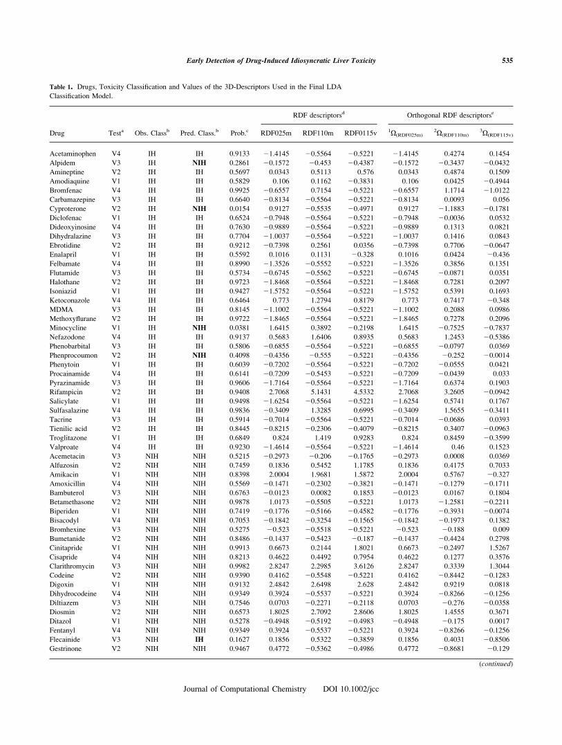
Table 1. Drugs, Toxicity Classification and Values of the 3D-Descriptors Used in the Final LDA

Classification Model.

Drug Testa Obs. Classb Pred. Class.b Prob.c

RDF descriptorsd Orthogonal RDF descriptorse

RDF025m RDF110m RDF0115v 1X(RDF025m)2X(RDF110m)

3X(RDF115v)

Acetaminophen V4 IH IH 0.9133 21.4145 20.5564 20.5221 21.4145 0.4274 0.1454

Alpidem V3 IH NIH 0.2861 20.1572 20.453 20.4387 20.1572 20.3437 20.0432

Amineptine V2 IH IH 0.5697 0.0343 0.5113 0.576 0.0343 0.4874 0.1509

Amodiaquine V1 IH IH 0.5829 0.106 0.1162 20.3831 0.106 0.0425 20.4944

Bromfenac V4 IH IH 0.9925 20.6557 0.7154 20.5221 20.6557 1.1714 21.0122

Carbamazepine V3 IH IH 0.6640 20.8134 20.5564 20.5221 20.8134 0.0093 0.056

Cyproterone V2 IH NIH 0.0154 0.9127 20.5535 20.4971 0.9127 21.1883 20.1781

Diclofenac V1 IH IH 0.6524 20.7948 20.5564 20.5221 20.7948 20.0036 0.0532

Dideoxyinosine V4 IH IH 0.7630 20.9889 20.5564 20.5221 20.9889 0.1313 0.0821

Dihydralazine V3 IH IH 0.7704 21.0037 20.5564 20.5221 21.0037 0.1416 0.0843

Ebrotidine V2 IH IH 0.9212 20.7398 0.2561 0.0356 20.7398 0.7706 20.0647

Enalapril V1 IH IH 0.5592 0.1016 0.1131 20.328 0.1016 0.0424 20.436

Felbamate V4 IH IH 0.8990 21.3526 20.5552 20.5221 21.3526 0.3856 0.1351

Flutamide V3 IH IH 0.5734 20.6745 20.5562 20.5221 20.6745 20.0871 0.0351

Halothane V2 IH IH 0.9723 21.8468 20.5564 20.5221 21.8468 0.7281 0.2097

Isoniazid V1 IH IH 0.9427 21.5752 20.5564 20.5221 21.5752 0.5391 0.1693

Ketoconazole V4 IH IH 0.6464 0.773 1.2794 0.8179 0.773 0.7417 20.348

MDMA V3 IH IH 0.8145 21.1002 20.5564 20.5221 21.1002 0.2088 0.0986

Methoxyflurane V2 IH IH 0.9722 21.8465 20.5564 20.5221 21.8465 0.7278 0.2096

Minocycline V1 IH NIH 0.0381 1.6415 0.3892 20.2198 1.6415 20.7525 20.7837

Nefazodone V4 IH IH 0.9137 0.5683 1.6406 0.8935 0.5683 1.2453 20.5386

Phenobarbital V3 IH IH 0.5806 20.6855 20.5564 20.5221 20.6855 20.0797 0.0369

Phenprocoumon V2 IH NIH 0.4098 20.4356 20.555 20.5221 20.4356 20.252 20.0014

Phenytoin V1 IH IH 0.6039 20.7202 20.5564 20.5221 20.7202 20.0555 0.0421

Procainamide V4 IH IH 0.6141 20.7209 20.5453 20.5221 20.7209 20.0439 0.033

Pyrazinamide V3 IH IH 0.9606 21.7164 20.5564 20.5221 21.7164 0.6374 0.1903

Rifampicin V2 IH IH 0.9408 2.7068 5.1431 4.5332 2.7068 3.2605 20.0942

Salicylate V1 IH IH 0.9498 21.6254 20.5564 20.5221 21.6254 0.5741 0.1767

Sulfasalazine V4 IH IH 0.9836 20.3409 1.3285 0.6995 20.3409 1.5655 20.3411

Tacrine V3 IH IH 0.5914 20.7014 20.5564 20.5221 20.7014 20.0686 0.0393

Tienilic acid V2 IH IH 0.8445 20.8215 20.2306 20.4079 20.8215 0.3407 20.0963

Troglitazone V1 IH IH 0.6849 0.824 1.419 0.9283 0.824 0.8459 20.3599

Valproate V4 IH IH 0.9230 21.4614 20.5564 20.5221 21.4614 0.46 0.1523

Acemetacin V3 NIH NIH 0.5215 20.2973 20.206 20.1765 20.2973 0.0008 0.0369

Alfuzosin V2 NIH NIH 0.7459 0.1836 0.5452 1.1785 0.1836 0.4175 0.7033

Amikacin V1 NIH NIH 0.8398 2.0004 1.9681 1.5872 2.0004 0.5767 20.327

Amoxicillin V4 NIH NIH 0.5569 20.1471 20.2302 20.3821 20.1471 20.1279 20.1711

Bambuterol V3 NIH NIH 0.6763 20.0123 0.0082 0.1853 20.0123 0.0167 0.1804

Betamethasone V2 NIH NIH 0.9878 1.0173 20.5505 20.5221 1.0173 21.2581 20.2211

Biperiden V1 NIH NIH 0.7419 20.1776 20.5166 20.4582 20.1776 20.3931 20.0074

Bisacodyl V4 NIH NIH 0.7053 20.1842 20.3254 20.1565 20.1842 20.1973 0.1382

Bromhexine V3 NIH NIH 0.5275 20.523 20.5518 20.5221 20.523 20.188 0.009

Bumetanide V2 NIH NIH 0.8486 20.1437 20.5423 20.187 20.1437 20.4424 0.2798

Cinitapride V1 NIH NIH 0.9913 0.6673 0.2144 1.8021 0.6673 20.2497 1.5267

Cisapride V4 NIH NIH 0.8213 0.4622 0.4492 0.7954 0.4622 0.1277 0.3576

Clarithromycin V3 NIH NIH 0.9982 2.8247 2.2985 3.6126 2.8247 0.3339 1.3044

Codeine V2 NIH NIH 0.9390 0.4162 20.5548 20.5221 0.4162 20.8442 20.1283

Digoxin V1 NIH NIH 0.9132 2.4842 2.6498 2.628 2.4842 0.9219 0.0818

Dihydrocodeine V4 NIH NIH 0.9349 0.3924 20.5537 20.5221 0.3924 20.8266 20.1256

Diltiazem V3 NIH NIH 0.7546 0.0703 20.2271 20.2118 0.0703 20.276 20.0358

Diosmin V2 NIH NIH 0.6573 1.8025 2.7092 2.8606 1.8025 1.4555 0.3671

Ditazol V1 NIH NIH 0.5278 20.4948 20.5192 20.4983 20.4948 20.175 0.0017

Fentanyl V4 NIH NIH 0.9349 0.3924 20.5537 20.5221 0.3924 20.8266 20.1256

Flecainide V3 NIH IH 0.1627 0.1856 0.5322 20.3859 0.1856 0.4031 20.8506

Gestrinone V2 NIH NIH 0.9467 0.4772 20.5362 20.4986 0.4772 20.8681 20.129

(continued)

535Early Detection of Drug-Induced Idiosyncratic Liver Toxicity


MM1 molecular mechanics force field. Structures were then

further optimized by the semiempirical molecular orbital pack-

age MOPAC 6.0.34 The PM3 Hamiltonian35 was used to obtain

minimal-energy geometry optimized structures, which in turn

were also checked by frequency calculations. RDF molecular

descriptors were then calculated at radii ranging from 1.0 to

15.5 A, with increments of 0.5 A, using the Dragon software

package.36 As weighting properties, we tried all the atomic prop-

erties available in the Dragon software (masses, van der Waals

volumes, Sanderson electronegativities and polarizabilities),

finally computing a total of 150 descriptors.30

LDA Classification Model

The task here is to find a classification function [eq. (2)] that

best describes the idiosyncratic hepatotoxicity IH, as a linear

combination of the predictor X-variables (the RDF descriptors)

weighed by the coefficients bk:

IH ¼ b0 þ b1 3 RDFx1 þ b2 3 RDFx2 þ � � � þ bk 3 RDFxk (2)

In developing this classification function, IH values of 11 and

21 were assigned to toxic and nontoxic drugs, respectively, and

the equation coefficients were obtained by the least squares

method as implemented in the general discriminant analysis

(GDA) module of the STATISTICA 6.0 software package.37 In

addition, all the predictor variables were standardized38 after

LDA modeling and the forward stepwise (FS) method was

selected as the strategy for variable selection.39

The quality of the final LDA model was established by

examining its discriminatory power—Wilk’s U statistic and the

square of Mahalanobis’s distance (D2), and statistical signifi-

cance—Fisher ratio (F) and p-level (p). The ratio between cases

and predictor variables (q value) was also inspected to avoid

over-fitting or chance correlation problems.38

Specifically, the Wilk’s U statistic for the overall discrimina-

tion is computed as the ratio of the determinant of the within-

groups variance/covariance matrix (W) over the determinant of

the total variance/covariance matrix (T)40:

U ¼ Det:ðWÞDet:ðTÞ (3)

The Mahalanobis distance is the distance of a case from the

centroid in the multidimensional space, defined by the correlated

independent variables. It is computed as follows40:

Table 1. (Continued)

Drug Testa Obs. Classb Pred. Class.b Prob.c

RDF descriptorsd Orthogonal RDF descriptorse

RDF025m RDF110m RDF0115v 1X(RDF025m)2X(RDF110m)

3X(RDF115v)

Gliclazide V1 NIH NIH 0.7733 20.2385 20.3543 0.0696 20.2385 20.1884 0.3961

Indapamide V4 NIH NIH 0.5774 20.3289 20.4541 20.5113 20.3289 20.2253 20.0894

Ketoprofen V3 NIH IH 0.4441 20.6493 20.5564 20.5221 20.6493 20.1048 0.0316

Ketotifen V2 NIH NIH 0.8720 0.1207 20.5564 20.5221 0.1207 20.6404 20.083

Loratadine V1 NIH NIH 0.8908 0.3206 20.3336 20.2744 0.3206 20.5566 20.0481

Mesterolone V4 NIH NIH 0.9486 0.479 20.5564 20.5221 0.479 20.8896 20.1363

Methylergometrine V3 NIH IH 0.4919 0.36 0.2405 20.3551 0.36 20.0099 20.6062

Nimodipine V2 NIH NIH 0.9176 0.3806 20.4408 20.4142 0.3806 20.7055 20.1087

Nitrendipine V1 NIH NIH 0.8862 0.1688 20.5564 20.5221 0.1688 20.6738 20.0901

Oxazepam V4 NIH NIH 0.5564 20.4872 20.5564 20.5221 20.4872 20.2176 0.0074

Pefloxacine V3 NIH NIH 0.9244 0.4004 20.4526 20.4169 0.4004 20.7311 20.1047

Penicillin V2 NIH NIH 0.5533 20.4688 20.4994 20.4402 20.4688 20.1733 0.0397

Quazepam V1 NIH NIH 0.7975 20.0587 20.5432 20.5221 20.0587 20.5024 20.0672

Quinapril V4 NIH NIH 0.9742 0.7621 20.4408 20.3245 0.7621 20.9709 20.0758

Retinol V3 NIH NIH 0.8121 0.0152 20.322 20.1292 0.0152 20.3326 0.1331

Tetracycline V2 NIH NIH 0.9934 1.2267 20.4368 20.2622 1.2267 21.29 20.0858

Tetrazepam V1 NIH NIH 0.7439 20.1854 20.5564 20.5221 20.1854 20.4275 20.0374

Ursodeoxycholic acid V4 NIH NIH 0.9237 1.0383 0.3361 0.2034 1.0383 20.3861 20.2271

Veralipride V3 NIH NIH 0.7652 0.0008 20.3041 20.2291 0.0008 20.3047 0.0206

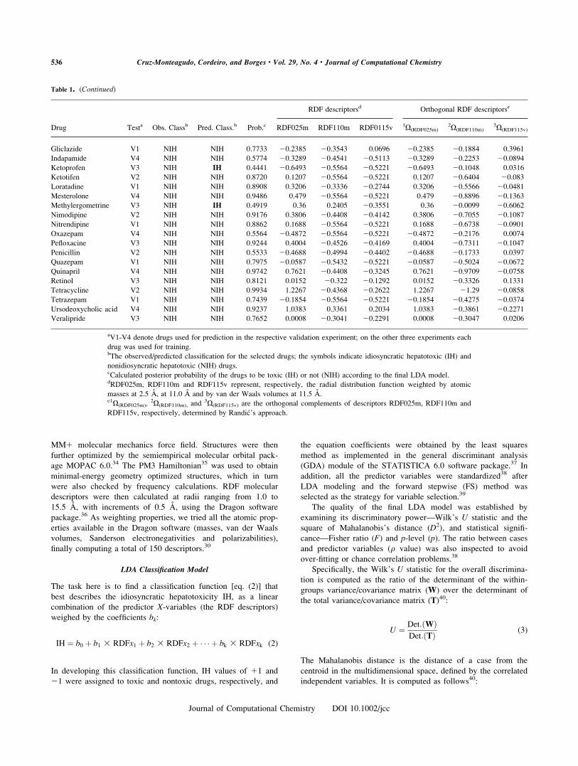
aV1-V4 denote drugs used for prediction in the respective validation experiment; on the other three experiments each

drug was used for training.bThe observed/predicted classification for the selected drugs; the symbols indicate idiosyncratic hepatotoxic (IH) and

nonidiosyncratic hepatotoxic (NIH) drugs.cCalculated posterior probability of the drugs to be toxic (IH) or not (NIH) according to the final LDA model.dRDF025m, RDF110m and RDF115v represent, respectively, the radial distribution function weighted by atomic

masses at 2.5 A, at 11.0 A and by van der Waals volumes at 11.5 A.e1X(RDF025m),

2X(RDF110m), and3X(RDF115v) are the orthogonal complements of descriptors RDF025m, RDF110m and

RDF115v, respectively, determined by Randic’s approach.



D ¼ ðn� 1Þ 3 ðXraw � XmeanÞ 3 C�1 3 ðXraw � XmeanÞ0 (4)

where Xraw and Xmean are the vectors of raw data and means

for the independent variables, respectively. C21 is the inverse of

the matrix of cross-products of deviations for the independent

variables, and n is the number of valid cases.

The F ratio is the statistic used here to test whether is statis-

tically significant the regression relation (the linear discriminant

analysis is a discrete variant of the multiple linear regression)

between the response variable IH and the set of RDF independ-

ent variables.

To choose between the null hypothesis (H0: b1 5 b2 5 . . . 5bk 5 0) where the regression relation is not statistically signifi-

cant, and the alternative hypothesis (Ha: not all bk equal zero)

where the independent variables are significantly included, we

use the ratio of the regression mean square (MSR) over the error

mean square (MSE) as the statistics for testing (F* 5 MSR/

MSE). The decision rule to control the Type I error for a confi-

dence interval 1 2 a at p 2 1 and n 2 p degrees of freedom is:

If F* � F (1 2 a; p 2 1, n 2 p) then one can not reject H0,

otherwise one should reject it, thereby accepting Ha.40

Here F*/F are the calculated and tabulated values of the

Fisher ratio, respectively; p is the number of adjustable parame-

ters and n is the total number of cases. At the same time, MSRand MSE are defined as follows:

MSR ¼ SSR

p� 1(5)

MSE ¼ SSE

n� p(6)

where SSR/SSE are the regression/error sum of squares, respec-

tively.

The value of the p-level represents a decreasing index of the

reliability of a result. The higher the p-level, the less we can

believe that the observed relation between variables in the sam-

ple is a reliable indicator of the relation between the respective

variables in the population. Specifically, the p-level represents

the probability of error that is involved in accepting our

observed result as valid, that is, as ‘‘representative of the popula-

tion’’.40

The q value represents the ratio between cases and adjustable

parameters on the equation and is defined as follows:

q ¼ n

p � g (7)

where n is the total number of cases, p is the number of adjusta-

ble parameters and g is the number of class or classification

groups. A value of q \ 4 can be considered as a warning value

of overfitting for a linear discriminant function.41

The performance of the model was verified by the Cooper’s

statistics—accuracy (it refers to the percentage of drugs, which

the model classifies correctly), sensitivity (percentage of toxic

drugs, which the model predicts to be toxic), specificity (percent-

age of nontoxic drugs, which the model predicts to be nontoxic),

positive predictivity (percentage of drugs predicted to be toxic by

the model that give positive results in vivo), negative predictivity

(percentage of drugs predicted to be nontoxic by the model that

give negative results in vivo), false positive rate or over-classifica-tion (percentage of nontoxic chemicals that are falsely predicted

to be toxic by the model), and false negative rate or under-classi-

fication (percentage of toxic chemicals that are falsely predicted

to be nontoxic by the model)—which are derived from the classi-

fication matrix generated by the LDA analysis.

It is well-known that if LDA, or any multiple linear-statisti-

cally based approach, is applied to data sets exhibiting collinear-

ity among the X-variables, the calculated coefficients are unsta-

ble and their interpretability breaks down. A practical approach

to avoid multicollinearity is the orthogonal descriptors technique

proposed by Randic.42,43 This technique also provides useful

structural input in building QSAR/QSTR relationships. Here we

used the Randic’s technique and orthogonalized the X-variablesfollowing the order selected by the FS method.

At last, validation of the classification model was checked

out by a resubstitution approach24,38: 25% of the total set of

compounds randomly selected as the predicting subset, and the

remaining compounds (75%) the training subset for carrying out

the first LDA classification (from now on this will be denoted

by Validation set 1: V1). Then, compounds in such subsets were

randomly interchanged three times, thus defining three new vali-

dation sets (V2, V3, and V4). The individual accuracy for each

training and predicting subset (V1–V4) and the overall average

values were finally estimated, the latter being the definitive mea-

sure of the robustness and predictivity of the full model.24,38

Artificial Neural Networks Classification Model

The use of nonparametric methods, like artificial neural net-

works (ANN),44 to solve the toxicological problem understudy

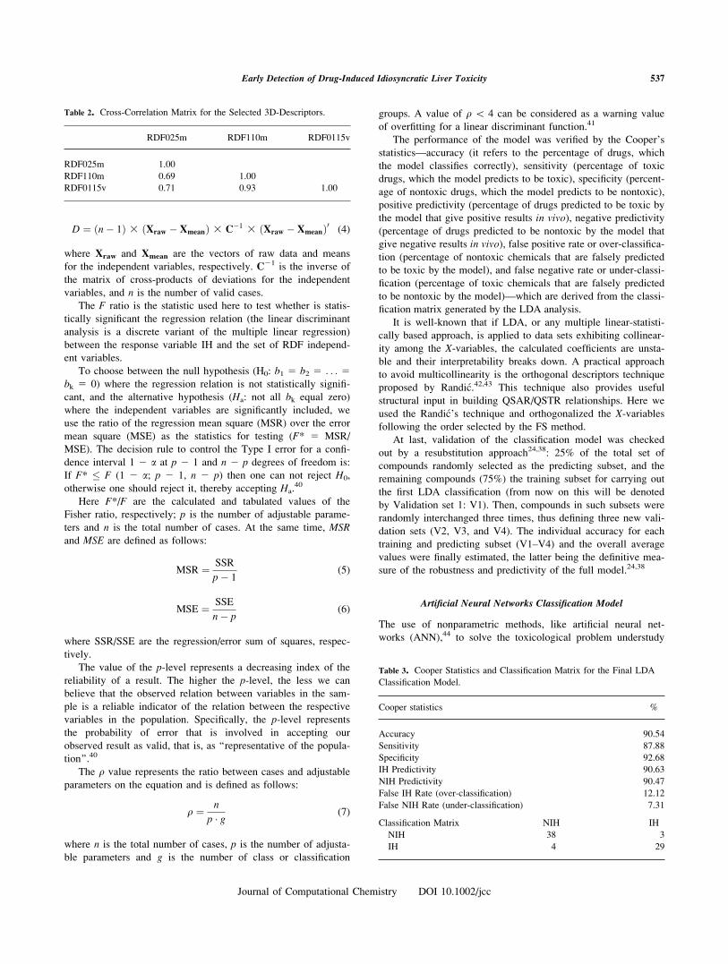
Table 2. Cross-Correlation Matrix for the Selected 3D-Descriptors.

RDF025m RDF110m RDF0115v

RDF025m 1.00

RDF110m 0.69 1.00

RDF0115v 0.71 0.93 1.00

Table 3. Cooper Statistics and Classification Matrix for the Final LDA

Classification Model.

Cooper statistics %

Accuracy 90.54

Sensitivity 87.88

Specificity 92.68

IH Predictivity 90.63

NIH Predictivity 90.47

False IH Rate (over-classification) 12.12

False NIH Rate (under-classification) 7.31

Classification Matrix NIH IH

NIH 38 3

IH 4 29



was investigated. Specifically, the ability of a classification

ANN model derived from the descriptors identified by FS-LDA

was evaluated. The model was built with the aid of STATIS-

TICA 6.037 using a Radial Basis Function (RBF) architecture.45

RBF networks combine a single radial hidden layer with a dot

product output layer. The hidden layer neurons act as clustering

centers, grouping similar training cases, and the output layer

forms a discriminant function. Since the clustering transforma-

tion is nonlinear, a linear output layer is sufficient to perform an

overall nonlinear function. These networks follow a two stage

training process, namely: (i) assignment of the radial centers and

their deviations and (ii) optimization of the output layer. The

quality of the RBF-ANN model was assessed by examining its

performance, errors and percentages of correctly classified IH/

NIH drugs in training and testing series, based on the distribu-

tion of compounds in the V1 set above referred to. Network

training was conducted by using 75% of the drugs (labeled with

V2, V3, or V4 on Table 1) and the remaining 25% of the drugs

(labeled with V1 on Table 1) were used for model testing.

Machine Learning Classification Algorithm

Here, the ability of the OneR classification algorithm,46 as

implemented in software WEKA (Waikato Environment for

Knowledge Analysis),46,47 to flag potential idiosyncratic hepato-

toxicity was tested. OneR, short for ‘‘One Rule’’, is a simple

machine learning classification algorithm that generates a one-

level decision tree. OneR is able to infer typically simple classi-

fication rules from a set of instances that are straightforward for

humans to interpret. This algorithm creates one rule for each at-

tribute in the training data, and then selects the best rule as its

‘‘one rule’’. To create a rule for a specific attribute, the most fre-

quent class for each attribute value must be determined. A rule

is thus simply a set of attribute values bound to their majority

class; the rule is based on such binding for each value of the at-

tribute. One can also define the error rate of a rule as the num-

ber of misclassified training data instances by using the rule.46

Typically machine learning algorithms select the rule with

the lowest error rate as the best one. If two or more rules

have the same error rate, the rule is chosen at random. In oppo-

sition, the OneR algorithm in WEKA picks the rule with the

highest number of correct instances, not the lowest error rate,

and does not randomly select a rule when error rates are identi-

cal. The best rule obtained was then validated by means of four-

fold cross internal validation (an iterative process of rederiving

the model leaving the 25% of the data out each time).

Desirability Analysis

Response/desirability profiling allows tracing the response sur-

face produced by fitting the observed responses using an equa-

tion based on levels of the predictor variables. The predicted

values for the dependent variable at different combinations of

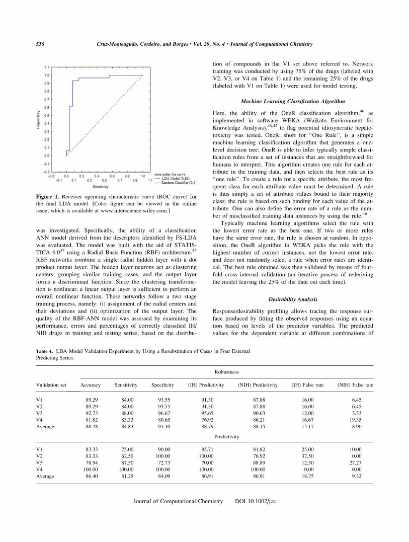
Figure 1. Receiver operating characteristic curve (ROC curve) for

the final LDA model. [Color figure can be viewed in the online

issue, which is available at www.interscience.wiley.com.]

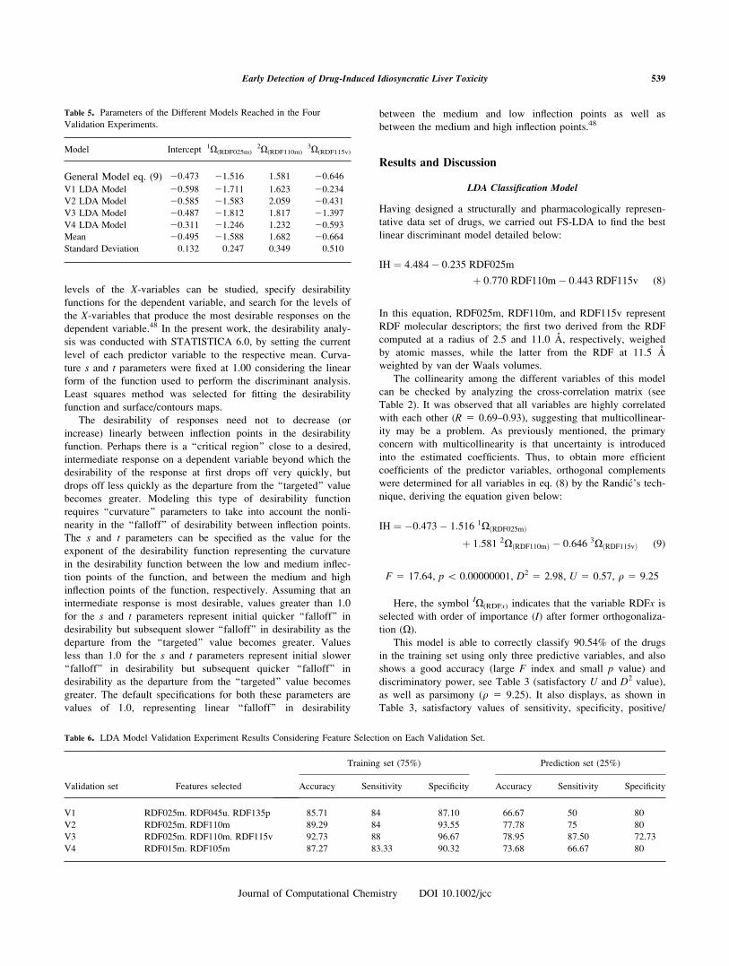
Table 4. LDA Model Validation Experiment by Using a Resubstitution of Cases in Four External

Predicting Series.

Validation set

Robustness

Accuracy Sensitivity Specificity (IH) Predictivity (NIH) Predictivity (IH) False rate (NIH) False rate

V1 89.29 84.00 93.55 91.30 87.88 16.00 6.45

V2 89.29 84.00 93.55 91.30 87.88 16.00 6.45

V3 92.73 88.00 96.67 95.65 90.63 12.00 3.33

V4 81.82 83.33 80.65 76.92 86.21 16.67 19.35

Average 88.28 84.83 91.10 88.79 88.15 15.17 8.90

Predictivity

V1 83.33 75.00 90.00 85.71 81.82 25.00 10.00

V2 83.33 62.50 100.00 100.00 76.92 37.50 0.00

V3 78.94 87.50 72.73 70.00 88.89 12.50 27.27

V4 100.00 100.00 100.00 100.00 100.00 0.00 0.00

Average 86.40 81.25 84.09 86.91 86.91 18.75 9.32



levels of the X-variables can be studied, specify desirability

functions for the dependent variable, and search for the levels of

the X-variables that produce the most desirable responses on the

dependent variable.48 In the present work, the desirability analy-

sis was conducted with STATISTICA 6.0, by setting the current

level of each predictor variable to the respective mean. Curva-

ture s and t parameters were fixed at 1.00 considering the linear

form of the function used to perform the discriminant analysis.

Least squares method was selected for fitting the desirability

function and surface/contours maps.

The desirability of responses need not to decrease (or

increase) linearly between inflection points in the desirability

function. Perhaps there is a ‘‘critical region’’ close to a desired,

intermediate response on a dependent variable beyond which the

desirability of the response at first drops off very quickly, but

drops off less quickly as the departure from the ‘‘targeted’’ value

becomes greater. Modeling this type of desirability function

requires ‘‘curvature’’ parameters to take into account the nonli-

nearity in the ‘‘falloff’’ of desirability between inflection points.

The s and t parameters can be specified as the value for the

exponent of the desirability function representing the curvature

in the desirability function between the low and medium inflec-

tion points of the function, and between the medium and high

inflection points of the function, respectively. Assuming that an

intermediate response is most desirable, values greater than 1.0

for the s and t parameters represent initial quicker ‘‘falloff’’ in

desirability but subsequent slower ‘‘falloff’’ in desirability as the

departure from the ‘‘targeted’’ value becomes greater. Values

less than 1.0 for the s and t parameters represent initial slower

‘‘falloff’’ in desirability but subsequent quicker ‘‘falloff’’ in

desirability as the departure from the ‘‘targeted’’ value becomes

greater. The default specifications for both these parameters are

values of 1.0, representing linear ‘‘falloff’’ in desirability

between the medium and low inflection points as well as

between the medium and high inflection points.48

Results and Discussion

LDA Classification Model

Having designed a structurally and pharmacologically represen-

tative data set of drugs, we carried out FS-LDA to find the best

linear discriminant model detailed below:

IH ¼ 4:484� 0:235 RDF025m

þ 0:770 RDF110m� 0:443 RDF115v (8)

In this equation, RDF025m, RDF110m, and RDF115v represent

RDF molecular descriptors; the first two derived from the RDF

computed at a radius of 2.5 and 11.0 A, respectively, weighed

by atomic masses, while the latter from the RDF at 11.5 A

weighted by van der Waals volumes.

The collinearity among the different variables of this model

can be checked by analyzing the cross-correlation matrix (see

Table 2). It was observed that all variables are highly correlated

with each other (R 5 0.69–0.93), suggesting that multicollinear-

ity may be a problem. As previously mentioned, the primary

concern with multicollinearity is that uncertainty is introduced

into the estimated coefficients. Thus, to obtain more efficient

coefficients of the predictor variables, orthogonal complements

were determined for all variables in eq. (8) by the Randic’s tech-

nique, deriving the equation given below:

IH ¼ �0:473� 1:516 1XðRDF025mÞþ 1:581 2XðRDF110mÞ � 0:646 3XðRDF115vÞ (9)

F 5 17.64, p\ 0.00000001, D2 5 2.98, U 5 0.57, q 5 9.25

Here, the symbol IX(RDFx) indicates that the variable RDFx is

selected with order of importance (I) after former orthogonaliza-

tion (X).This model is able to correctly classify 90.54% of the drugs

in the training set using only three predictive variables, and also

shows a good accuracy (large F index and small p value) and

discriminatory power, see Table 3 (satisfactory U and D2 value),

as well as parsimony (q 5 9.25). It also displays, as shown in

Table 3, satisfactory values of sensitivity, specificity, positive/

Table 5. Parameters of the Different Models Reached in the Four

Validation Experiments.

Model Intercept 1X(RDF025m)2X(RDF110m)

3X(RDF115v)

General Model eq. (9) 20.473 21.516 1.581 20.646

V1 LDA Model 20.598 21.711 1.623 20.234

V2 LDA Model 20.585 21.583 2.059 20.431

V3 LDA Model 20.487 21.812 1.817 21.397

V4 LDA Model 20.311 21.246 1.232 20.593

Mean 20.495 21.588 1.682 20.664

Standard Deviation 0.132 0.247 0.349 0.510

Table 6. LDA Model Validation Experiment Results Considering Feature Selection on Each Validation Set.

Validation set Features selected

Training set (75%) Prediction set (25%)

Accuracy Sensitivity Specificity Accuracy Sensitivity Specificity

V1 RDF025m. RDF045u. RDF135p 85.71 84 87.10 66.67 50 80

V2 RDF025m. RDF110m 89.29 84 93.55 77.78 75 80

V3 RDF025m. RDF110m. RDF115v 92.73 88 96.67 78.95 87.50 72.73

V4 RDF015m. RDF105m 87.27 83.33 90.32 73.68 66.67 80



negative predictivity, and false positive/negative rates (over/

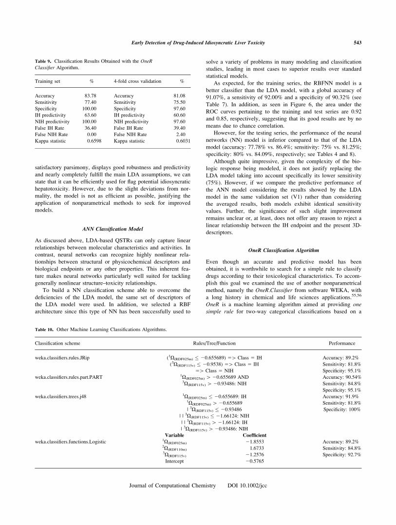
under-classification). In addition, the receiver operating charac-

teristic curve (ROC curve) obtained, indicate that the model is

not a random, but a statistically significant, classifier. A ROC

curve49,50 plots the sensitivity versus one minus the specificity.

An ideal classifier hugs the left side and top side of the graph,

and the area under the curve is 1.0. A random classifier should

achieve �0.5 (Fig. 1).

Validation of the model was undertaken by the re-substitution

technique24,51 and the results derived for four different valida-

tion subsets are summarized in Table 4. Judging from the aver-

aged values of accuracy in the training/test subsets (88.28%/

86.40%), as well as of sensitivity, specificity, etc., the model is

robust, exhibits little dependence on the composition of the

training and test subsets, and has high predictive ability.

Since selection of test compounds from the full set is ran-

dom, we replicate four times the selection by including other

compounds than the previously selected in order to access the

influence of the test set variation over the performance of the

model. As shown in Table 4, the performance in the different

validation experiments showed slight variations. For this reason,

we report averaged values which are a more representative mea-

sure of the performance of the model. In Table 5, one can notice

the stability of model parameters for each validation experiment

contrasted to the general model.

Additionally, the robustness of the model proposed is verified

by re-doing the descriptor selection and line fitting with 75%

compounds without touching the remaining 25% compounds.

After the model is developed, the 25% compounds were used to

test the predictive ability of the model. This procedure is carried

out on the four validation sets. By looking at Table 6, one can

see that the descriptors selected each time are similar and pre-

diction results are in the similar range, which confirms the

robustness of the model.

Anyhow, the definitive measure of the predictive ability of

any model can only be assessed by using an independent set of

drugs never used for training, as carried out afterwards.

The next step is to find out if the basic assumptions of LDA

are fulfilled.38,52 As the names implies, LDA establishes a linear,

additive relationship between the molecular descriptors and the

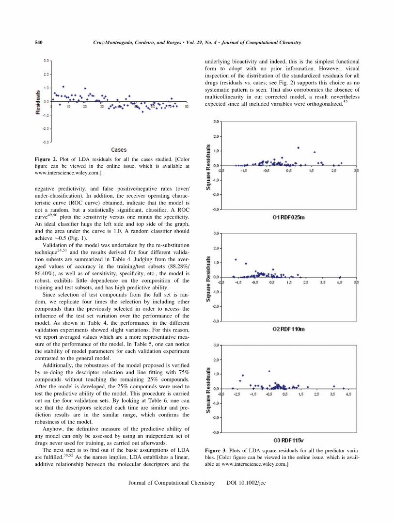
underlying bioactivity and indeed, this is the simplest functional

form to adopt with no prior information. However, visual

inspection of the distribution of the standardized residuals for all

drugs (residuals vs. cases; see Fig. 2) supports this choice as no

systematic pattern is seen. That also corroborates the absence of

multicollinearity in our corrected model, a result nevertheless

expected since all included variables were orthogonalized.52

Figure 2. Plot of LDA residuals for all the cases studied. [Color

figure can be viewed in the online issue, which is available at

www.interscience.wiley.com.]

Figure 3. Plots of LDA square residuals for all the predictor varia-

bles. [Color figure can be viewed in the online issue, which is avail-

able at www.interscience.wiley.com.]



Now, we must check the parametric assumption of homosce-

dasticity (i.e.: homogeneity of variance of the variables), which

if not satisfied invalidates extrapolations from the model.52 A

simple method to detect heteroscedasticity in large data sets is

by inspecting the plots of the residuals for each variable

included in the model. In reality, when no prior or heuristic in-

formation concerning to the heteroscedasticity exist, one might

develop the model under the assumption of homoscedasticity,

and then perform a post mortem analysis of the squares residuals

of the variables included in the model to detect any systematic

or consistent pattern. If such a pattern is detected, then we can

conclude that our variables are not homoscedastics. The plots in

Figure 3 reveal a greater scatter on the points, without any con-

sistent pattern, validating a posteriori the preadopted assumption

of homoscedasticity.

Moving on to the last important parametric assumption of

LDA, i.e.: multivariate normality. This seems to be the only

weak point of our model. First, not all the model predictor varia-

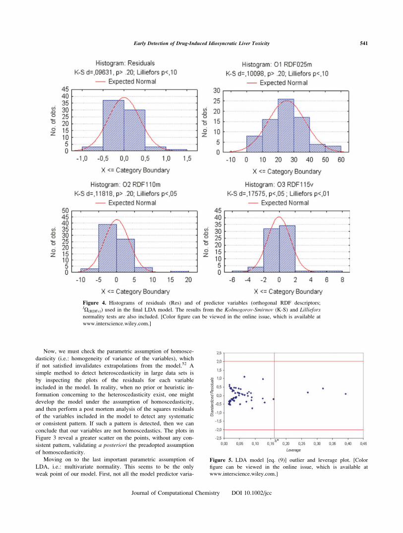
Figure 4. Histograms of residuals (Res) and of predictor variables (orthogonal RDF descriptors;IX(RDFx)) used in the final LDA model. The results from the Kolmogorov-Smirnov (K-S) and Lillieforsnormality tests are also included. [Color figure can be viewed in the online issue, which is available at


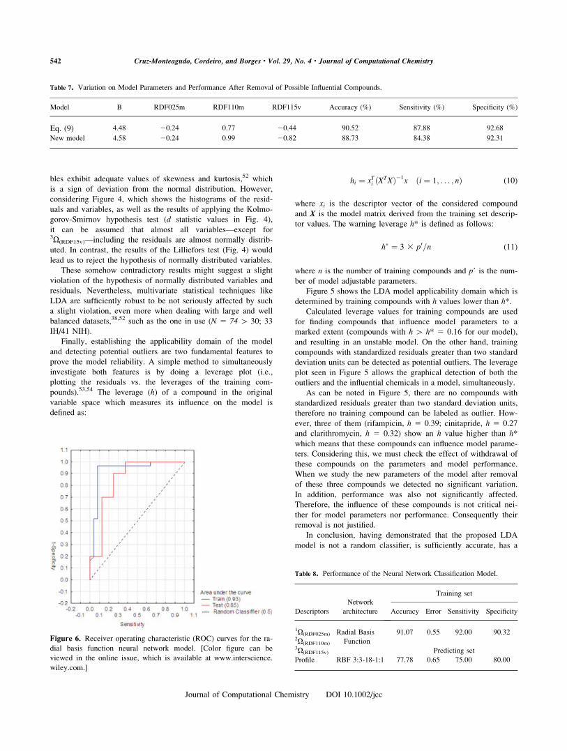
Figure 5. LDA model [eq. (9)] outlier and leverage plot. [Color

figure can be viewed in the online issue, which is available at




bles exhibit adequate values of skewness and kurtosis,52 which

is a sign of deviation from the normal distribution. However,

considering Figure 4, which shows the histograms of the resid-

uals and variables, as well as the results of applying the Kolmo-

gorov-Smirnov hypothesis test (d statistic values in Fig. 4),

it can be assumed that almost all variables—except for3X(RDF15v)—including the residuals are almost normally distrib-

uted. In contrast, the results of the Lilliefors test (Fig. 4) would

lead us to reject the hypothesis of normally distributed variables.

These somehow contradictory results might suggest a slight

violation of the hypothesis of normally distributed variables and

residuals. Nevertheless, multivariate statistical techniques like

LDA are sufficiently robust to be not seriously affected by such

a slight violation, even more when dealing with large and well

balanced datasets,38,52 such as the one in use (N 5 74 [ 30; 33

IH/41 NIH).

Finally, establishing the applicability domain of the model

and detecting potential outliers are two fundamental features to

prove the model reliability. A simple method to simultaneously

investigate both features is by doing a leverage plot (i.e.,

plotting the residuals vs. the leverages of the training com-

pounds).53,54 The leverage (h) of a compound in the original

variable space which measures its influence on the model is

defined as:

hi ¼ xTi ðXTXÞ�1x ði ¼ 1; . . . ; nÞ (10)

where xi is the descriptor vector of the considered compound

and X is the model matrix derived from the training set descrip-

tor values. The warning leverage h* is defined as follows:

h� ¼ 3 3 p0=n (11)

where n is the number of training compounds and p’ is the num-

ber of model adjustable parameters.

Figure 5 shows the LDA model applicability domain which is

determined by training compounds with h values lower than h*.Calculated leverage values for training compounds are used

for finding compounds that influence model parameters to a

marked extent (compounds with h [ h* 5 0.16 for our model),

and resulting in an unstable model. On the other hand, training

compounds with standardized residuals greater than two standard

deviation units can be detected as potential outliers. The leverage

plot seen in Figure 5 allows the graphical detection of both the

outliers and the influential chemicals in a model, simultaneously.

As can be noted in Figure 5, there are no compounds with

standardized residuals greater than two standard deviation units,

therefore no training compound can be labeled as outlier. How-

ever, three of them (rifampicin, h 5 0.39; cinitapride, h 5 0.27

and clarithromycin, h 5 0.32) show an h value higher than h*which means that these compounds can influence model parame-

ters. Considering this, we must check the effect of withdrawal of

these compounds on the parameters and model performance.

When we study the new parameters of the model after removal

of these three compounds we detected no significant variation.

In addition, performance was also not significantly affected.

Therefore, the influence of these compounds is not critical nei-

ther for model parameters nor performance. Consequently their

removal is not justified.

In conclusion, having demonstrated that the proposed LDA

model is not a random classifier, is sufficiently accurate, has a

Table 7. Variation on Model Parameters and Performance After Removal of Possible Influential Compounds.

Model B RDF025m RDF110m RDF115v Accuracy (%) Sensitivity (%) Specificity (%)

Eq. (9) 4.48 20.24 0.77 20.44 90.52 87.88 92.68

New model 4.58 20.24 0.99 20.82 88.73 84.38 92.31

Figure 6. Receiver operating characteristic (ROC) curves for the ra-

dial basis function neural network model. [Color figure can be

viewed in the online issue, which is available at www.interscience.

wiley.com.]

Table 8. Performance of the Neural Network Classification Model.

Descriptors

Network

architecture

Training set

Accuracy Error Sensitivity Specificity

1X(RDF025m)2X(RDF110m)

Radial Basis

Function

91.07 0.55 92.00 90.32

3X(RDF115v) Predicting set

Profile RBF 3:3-18-1:1 77.78 0.65 75.00 80.00



satisfactory parsimony, displays good robustness and predictivity

and nearly completely fulfill the main LDA assumptions, we can

state that it can be efficiently used for flag potential idiosyncratic

hepatotoxicity. However, due to the slight deviations from nor-

mality, the model is not as efficient as possible, justifying the

application of nonparametrical methods to seek for improved

models.

ANN Classification Model

As discussed above, LDA-based QSTRs can only capture linear

relationships between molecular characteristics and activities. In

contrast, neural networks can recognize highly nonlinear rela-

tionships between structural or physicochemical descriptors and

biological endpoints or any other properties. This inherent fea-

ture makes neural networks particularly well suited for tackling

generally nonlinear structure–toxicity relationships.

To build a NN classification scheme able to overcome the

deficiencies of the LDA model, the same set of descriptors of

the LDA model were used. In addition, we selected a RBF

architecture since this type of NN has been successfully used to

solve a variety of problems in many modeling and classification

studies, leading in most cases to superior results over standard

statistical models.

As expected, for the training series, the RBFNN model is a

better classifier than the LDA model, with a global accuracy of

91.07%, a sensitivity of 92.00% and a specificity of 90.32% (see

Table 7). In addition, as seen in Figure 6, the area under the

ROC curves pertaining to the training and test series are 0.92

and 0.85, respectively, suggesting that its good results are by no

means due to chance correlation.

However, for the testing series, the performance of the neural

networks (NN) model is inferior compared to that of the LDA

model (accuracy: 77.78% vs. 86.4%; sensitivity: 75% vs. 81.25%;

specificity: 80% vs. 84.09%, respectively; see Tables 4 and 8).

Although quite impressive, given the complexity of the bio-

logic response being modeled, it does not justify replacing the

LDA model taking into account specifically its lower sensitivity

(75%). However, if we compare the predictive performance of

the ANN model considering the results showed by the LDA

model in the same validation set (V1) rather than considering

the averaged results, both models exhibit identical sensitivity

values. Further, the significance of such slight improvement

remains unclear or, at least, does not offer any reason to reject a

linear relationship between the IH endpoint and the present 3D-

descriptors.

OneR Classification Algorithm

Even though an accurate and predictive model has been

obtained, it is worthwhile to search for a simple rule to classify

drugs according to their toxicological characteristics. To accom-

plish this goal we examined the use of another nonparametrical

method, namely the OneR.Classifier from software WEKA, with

a long history in chemical and life sciences applications.55,56

OneR is a machine learning algorithm aimed at providing onesimple rule for two-way categorical classifications based on a

Table 9. Classification Results Obtained with the OneR

Classifier Algorithm.

Training set % 4-fold cross validation %

Accuracy 83.78 Accuracy 81.08

Sensitivity 77.40 Sensitivity 75.50

Specificity 100.00 Specificity 97.60

IH predictivity 63.60 IH predictivity 60.60

NIH predictivity 100.00 NIH predictivity 97.60

False IH Rate 36.40 False IH Rate 39.40

False NIH Rate 0.00 False NIH Rate 2.40

Kappa statistic 0.6598 Kappa statistic 0.6031

Table 10. Other Machine Learning Classifications Algorithms.

Classification scheme Rules/Tree/Function Performance

weka.classifiers.rules.JRip (1X(RDF025m) � 20.655689) 5[ Class 5 IH Accuracy: 89.2%

(3X(RDF115v) � 20.9538) 5[ Class 5 IH Sensitivity: 81.8%

5[ Class 5 NIH Specificity: 95.1%

weka.classifiers.rules.part.PART 1X(RDF025m) [20.655689 AND Accuracy: 90.54%3X(RDF115v) [20.93486: NIH Sensitivity: 84.8%

Specificity: 95.1%

weka.classifiers.trees.j48 1X(RDF025m) � 20.655689: IH Accuracy: 91.9%1X(RDF025m) [20.655689 Sensitivity: 81.8%

| 3X(RDF115v) � 20.93486 Specificity: 100%

| | 3X(RDF115v) � 21.66124: NIH

| | 3X(RDF115v) [21.66124: IH

| 3X(RDF115v) [20.93486: NIH

Variable Coefficient

weka.classifiers.functions.Logistic 1X(RDF025m) 21.8553 Accuracy: 89.2%2X(RDF110m) 1.6733 Sensitivity: 84.8%3X(RDF115v) 21.2576 Specificity: 92.7%

Intercept 20.5765



single parameter or molecular descriptor. The descriptor used

here was 1X(RDF025m), which is the more significant variable

included in the LDA model.

The One Rule for classifying the current drugs as IH or NIH

was found to be:

IF1X(RDF025m) \20.652517515, THEN CLASS 5 IH

OTHERWISE, THEN CLASS 5 NIH

It allows for a correct classification of 62 out of the 74 drugs

(83.78% of accuracy) from the training sample. To be more spe-

cific, 77.4% of the IH drugs and all the NIH drugs were classi-

fied correctly. Moreover, good overall predictability (81.08%)

and sensitivity/specificity (75.5%/97.6%, respectively) is found,

as judged by fourfold internal cross validation (see Table 9).

In conclusion, this one rule displays a good overall perform-

ance but has a rather low sensitivity. This last is the most impor-

tant feature when aiming at detecting potential IH drugs in early

drug development, since the consequences of misclassify an IH

drug (classify an IH drug as NIH) can be more devastating (the

false safe drug can reach the market with a potential risk to

human life) than the opposite case (classify an NIH drug as IH).

So, a potential drug is unnecessarily eliminated and will never

reach the market; it is regrettable but instead no life is compro-

mised.

Other rules or algorithms can be developed by using the

other two variables included in the LDA model. However, no

significant improvement is reached through more complex

schemes (see Table 10).

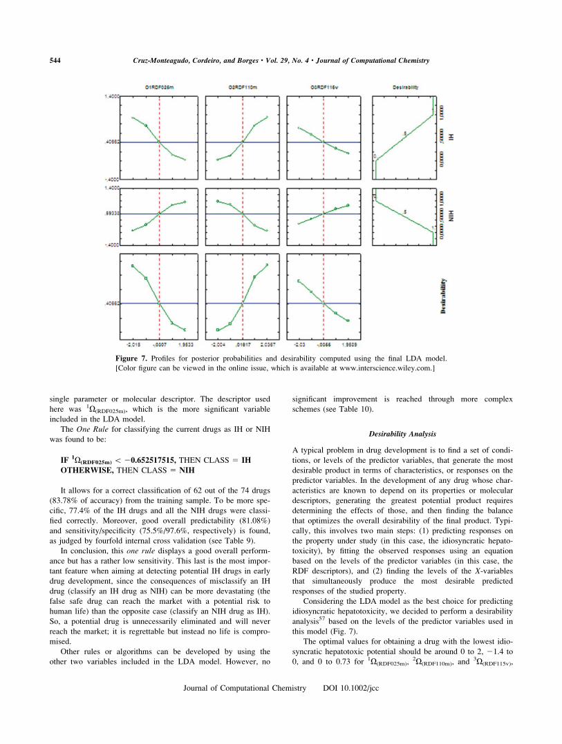
Desirability Analysis

A typical problem in drug development is to find a set of condi-

tions, or levels of the predictor variables, that generate the most

desirable product in terms of characteristics, or responses on the

predictor variables. In the development of any drug whose char-

acteristics are known to depend on its properties or molecular

descriptors, generating the greatest potential product requires

determining the effects of those, and then finding the balance

that optimizes the overall desirability of the final product. Typi-

cally, this involves two main steps: (1) predicting responses on

the property under study (in this case, the idiosyncratic hepato-

toxicity), by fitting the observed responses using an equation

based on the levels of the predictor variables (in this case, the

RDF descriptors), and (2) finding the levels of the X-variablesthat simultaneously produce the most desirable predicted

responses of the studied property.

Considering the LDA model as the best choice for predicting

idiosyncratic hepatotoxicity, we decided to perform a desirability

analysis57 based on the levels of the predictor variables used in

this model (Fig. 7).

The optimal values for obtaining a drug with the lowest idio-

syncratic hepatotoxic potential should be around 0 to 2, 21.4 to

0, and 0 to 0.73 for 1X(RDF025m),2X(RDF110m), and

3X(RDF115v),

Figure 7. Profiles for posterior probabilities and desirability computed using the final LDA model.

[Color figure can be viewed in the online issue, which is available at www.interscience.wiley.com.]



respectively, fixing the other two variables at their present mean

values (see Fig. 6). However, if the three variables are used at

their current values, it is possible to obtain a drug with a low

desirability value of 0.374 for the propensity to induce IH. On

the contrary, if the same current (mean) values are used it is

possible to obtain a drug with a desirability value of 0.626 for

the propensity to not induce IH.

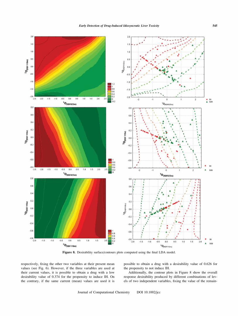
Additionally, the contour plots in Figure 8 show the overall

response desirability produced by different combinations of lev-

els of two independent variables, fixing the value of the remain-

Figure 8. Desirability surface/contours plots computed using the final LDA model.



ing third variable at its mean value. They were built by previ-

ously transforming scores of each of the three variables into

desirability scores that could range from 0.0 (undesirable; repre-

sented in green) to 1.0 (very desirable; represented in red). This

means that the green zone in the contour plots represents the

zone of higher probability to obtain a drug with lower potential

to induce an idiosyncratic hepatotoxic event, and the opposite

for the red zone. As can be noticed, most of the cases are

located in the proper zone of the plane, i.e.: most of the IH

drugs lay in the red (toxic) zone where the desirability values

are clearly over 0.75 while the NIH drugs lay in the green (safe)

zone where the desirability values are clearly under 0.3. The

maximum overlapping zones (between IH and NIH drugs) are

the zones with medium desirability values (ca. 0.5). The consis-

tence between the results from the desirability analysis and the

location of cases in the contour plots further demonstrates the

advantages of using this kind of analysis in drug development.

In Silico Virtual Screening: A Case Study

In an effort to illustrate the applicability of the method proposed

to the drug development process and at the same time to test its

predictive ability an external set of three pairs of chemically and

pharmacological related drugs having an observed opposite toxi-

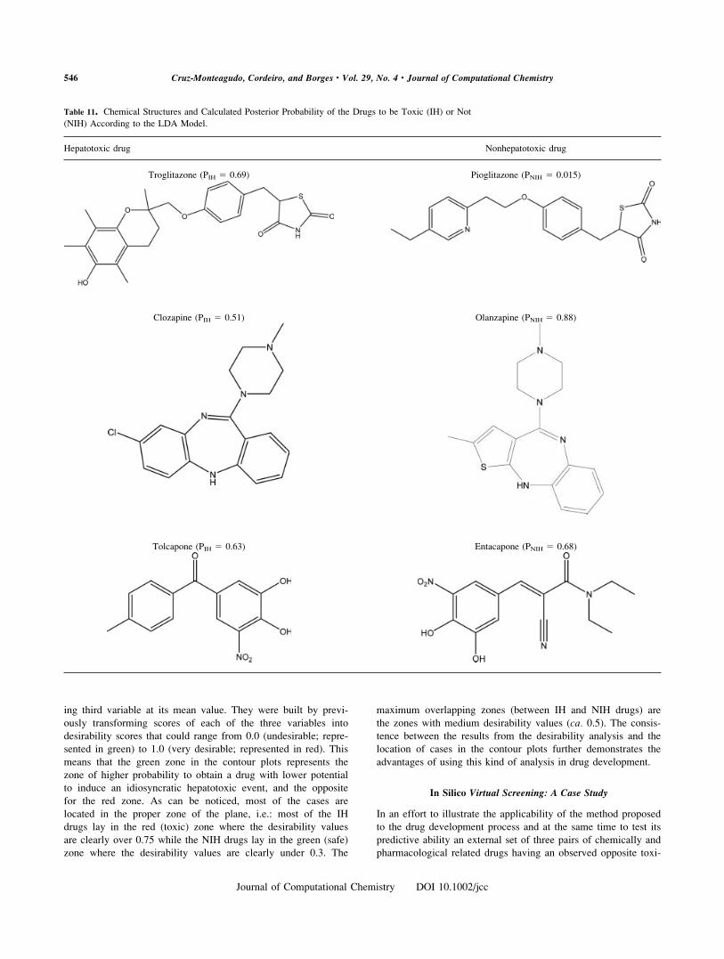
Table 11. Chemical Structures and Calculated Posterior Probability of the Drugs to be Toxic (IH) or Not

(NIH) According to the LDA Model.

Hepatotoxic drug Nonhepatotoxic drug

Troglitazone (PIH 5 0.69) Pioglitazone (PNIH 5 0.015)

Clozapine (PIH 5 0.51) Olanzapine (PNIH 5 0.88)

Tolcapone (PIH 5 0.63) Entacapone (PNIH 5 0.68)



cological profile (not used here for training), namely the pairs

troglitazone vs. pioglitazone, tolcapone vs. entacapone, and clo-

zapine vs. olanzapine, were used.

Thiazolidinediones or glitazones specifically target insulin re-

sistance. However, troglitazone, the first compound approved by

the FDA in the United States, proved to be hepatotoxic and was

withdrawn from the market after the report of several dozens of

deaths or cases of severe hepatic failure requiring liver trans-

plantation.58–61 In contrast, just a few cases of severe hepatotox-

icity have been reported with pioglitazone,62–64 consequently

this drug has not yet been recognized as hepatotoxic and is con-

sidered safe in the treatment of type 2 diabets.

On the other hand, two psychotropic drugs (clozapine and

olanzapine) provide another example. Although the main side

effects reported to clozapine is the agranulocytosis, its liver tox-

icity is also significant and life threatening.65,66 In opposition,

olanzapine is considered as a safe drug.67

Another case of similar drugs with different toxic profiles is

tolcapone and entacapone. Both are catechol-O-methyltransfer-

ase (COMT) inhibitors and were developed during the 1990’s to

be used as adjuncts to levodopa (LD)—dopa decarboxylase

(DDC) inhibitors in the treatment of Parkinson’s disease. Enta-

capone is currently in wide clinical use, while tolcapone can be

used in restricted indications only, due to its hepatotoxicity.68

The bioactivation and hepatotoxicity of this type of nitroaro-

matics drugs is currently under study.69 The chemical structures

among the calculated posterior probability of the drugs to be

toxic (IH) or not (NIH) according to the LDA model are shown

in Table 11.

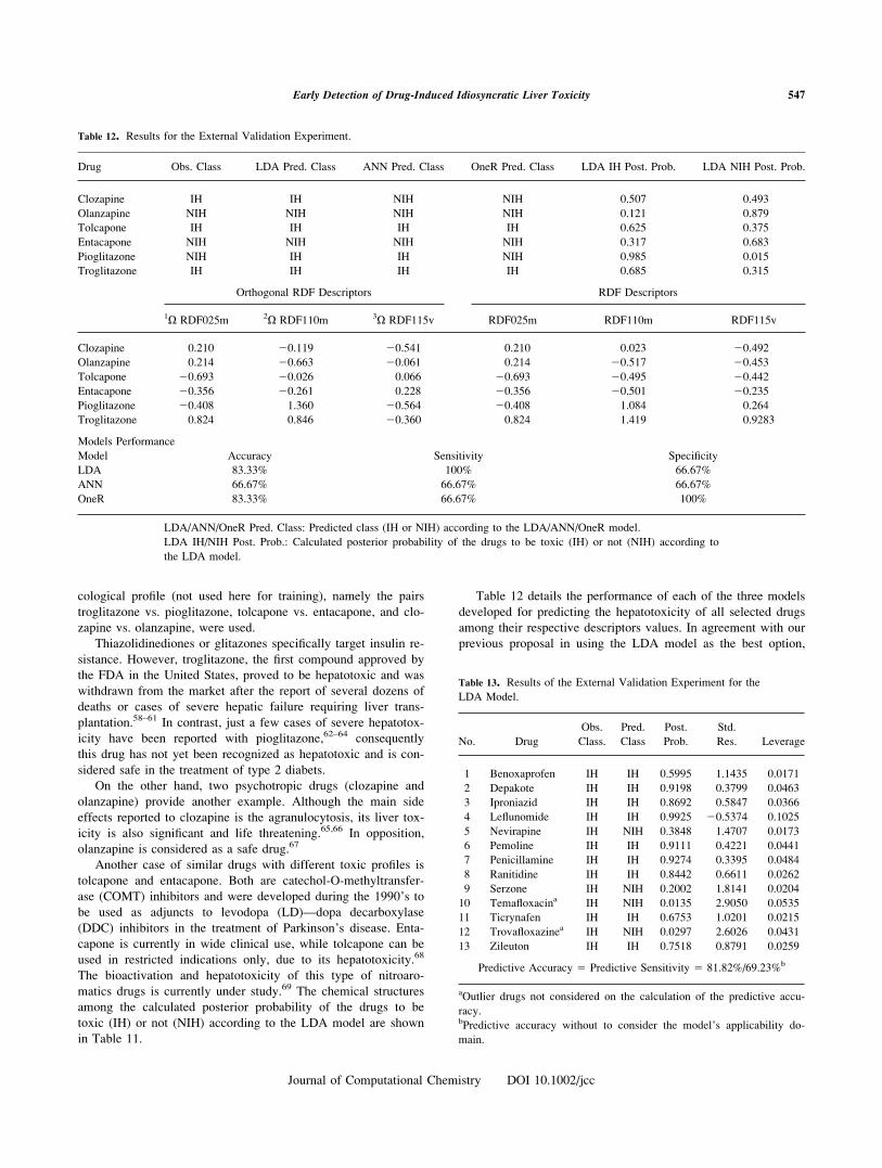
Table 12 details the performance of each of the three models

developed for predicting the hepatotoxicity of all selected drugs

among their respective descriptors values. In agreement with our

previous proposal in using the LDA model as the best option,

Table 12. Results for the External Validation Experiment.

Drug Obs. Class LDA Pred. Class ANN Pred. Class OneR Pred. Class LDA IH Post. Prob. LDA NIH Post. Prob.

Clozapine IH IH NIH NIH 0.507 0.493

Olanzapine NIH NIH NIH NIH 0.121 0.879

Tolcapone IH IH IH IH 0.625 0.375

Entacapone NIH NIH NIH NIH 0.317 0.683

Pioglitazone NIH IH IH NIH 0.985 0.015

Troglitazone IH IH IH IH 0.685 0.315

Orthogonal RDF Descriptors RDF Descriptors

1X RDF025m 2X RDF110m 3X RDF115v RDF025m RDF110m RDF115v

Clozapine 0.210 20.119 20.541 0.210 0.023 20.492

Olanzapine 0.214 20.663 20.061 0.214 20.517 20.453

Tolcapone 20.693 20.026 0.066 20.693 20.495 20.442

Entacapone 20.356 20.261 0.228 20.356 20.501 20.235

Pioglitazone 20.408 1.360 20.564 20.408 1.084 0.264

Troglitazone 0.824 0.846 20.360 0.824 1.419 0.9283

Models Performance

Model Accuracy Sensitivity Specificity

LDA 83.33% 100% 66.67%

ANN 66.67% 66.67% 66.67%

OneR 83.33% 66.67% 100%

LDA/ANN/OneR Pred. Class: Predicted class (IH or NIH) according to the LDA/ANN/OneR model.

LDA IH/NIH Post. Prob.: Calculated posterior probability of the drugs to be toxic (IH) or not (NIH) according to

the LDA model.

Table 13. Results of the External Validation Experiment for the

LDA Model.

No. Drug

Obs.

Class.

Pred.

Class

Post.

Prob.

Std.

Res. Leverage

1 Benoxaprofen IH IH 0.5995 1.1435 0.0171

2 Depakote IH IH 0.9198 0.3799 0.0463

3 Iproniazid IH IH 0.8692 0.5847 0.0366

4 Leflunomide IH IH 0.9925 20.5374 0.1025

5 Nevirapine IH NIH 0.3848 1.4707 0.0173

6 Pemoline IH IH 0.9111 0.4221 0.0441

7 Penicillamine IH IH 0.9274 0.3395 0.0484

8 Ranitidine IH IH 0.8442 0.6611 0.0262

9 Serzone IH NIH 0.2002 1.8141 0.0204

10 Temafloxacina IH NIH 0.0135 2.9050 0.0535

11 Ticrynafen IH IH 0.6753 1.0201 0.0215

12 Trovafloxazinea IH NIH 0.0297 2.6026 0.0431

13 Zileuton IH IH 0.7518 0.8791 0.0259

Predictive Accuracy 5 Predictive Sensitivity 5 81.82%/69.23%b

aOutlier drugs not considered on the calculation of the predictive accu-

racy.bPredictive accuracy without to consider the model’s applicability do-

main.



one can see that this model again shows the best performance of

the three evaluated models. Notice that the ANN model and

OneR classification algorithm were able to predict more than 60

and 80% of the data used, respectively. These results further

confirm the reliability of the three classification methods devel-

oped in the present work.

Is interesting to note that the only misclassified drug by the

LDA model was pioglitazone which is reasonable since until

today remains unclear whether or not its hepatotoxicity is a class

effect or it is related to the unique tocopherol side chain of tro-

glitazone.58 In addition, though not significant in number, some

reports of hepatotoxicity have been made for this drug.62,64 So,

we cannot be certain about the ‘‘misclassification’’ of the model

for this drug.

Another fact in support of the suitability of the LDA model

is that the leverage value of all drugs do not exceed the h* criti-

cal value of 0.16 (htolcapone 5 0.02; hentacapone 5 0.02; holanzapine5 0.02; hclozapine 5 0.04; hpioglitazone 5 0.09; htroglitazone 50.05), which means that these drugs fall within the applicability

domain of the model and so the predictions are reliable.

Since the data previously analyzed is insufficient for external

model evaluation, we decided to use a collection of 13 published

drugs causing idiosyncratic liver toxicity not included in the

training list. Such drugs can be found in the Physicians’ Desk

Reference and on the FDA website.70 Table 13 lists the names

of the idiosyncratic hepatotoxic drugs used as well as the respec-

tive predicted LDA classifications.

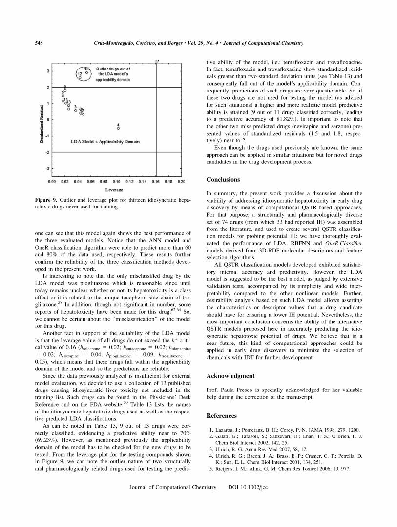
As can be noted in Table 13, 9 out of 13 drugs were cor-

rectly classified, evidencing a predictive ability near to 70%

(69.23%). However, as mentioned previously the applicability

domain of the model has to be checked for the new drugs to be

tested. From the leverage plot for the testing compounds shown

in Figure 9, we can note the outlier nature of two structurally

and pharmacologically related drugs used for testing the predic-

tive ability of the model, i.e.: temafloxacin and trovafloxacine.

In fact, temafloxacin and trovafloxacine show standardized resid-

uals greater than two standard deviation units (see Table 13) and

consequently fall out of the model’s applicability domain. Con-

sequently, predictions of such drugs are very questionable. So, if

these two drugs are not used for testing the model (as advised

for such situations) a higher and more realistic model predictive

ability is attained (9 out of 11 drugs classified correctly, leading

to a predictive accuracy of 81.82%). Is important to note that

the other two miss predicted drugs (nevirapine and sarzone) pre-

sented values of standardized residuals (1.5 and 1.8, respec-

tively) near to 2.

Even though the drugs used previously are known, the same

approach can be applied in similar situations but for novel drugs

candidates in the drug development process.

Conclusions

In summary, the present work provides a discussion about the

viability of addressing idiosyncratic hepatotoxicity in early drug

discovery by means of computational QSTR-based approaches.

For that purpose, a structurally and pharmacologically diverse

set of 74 drugs (from which 33 had reported IH) was assembled

from the literature, and used to create several QSTR classifica-

tion models for probing potential IH: we have thoroughly eval-

uated the performance of LDA, RBFNN and OneR.Classifiermodels derived from 3D-RDF molecular descriptors and feature

selection algorithms.

All QSTR classification models developed exhibited satisfac-

tory internal accuracy and predictivity. However, the LDA

model is suggested to be the best model, as judged by extensive

validation tests, accompanied by its simplicity and wide inter-

pretability compared to the other nonlinear models. Further,

desirability analysis based on such LDA model allows asserting

the characteristics or descriptor values that a drug candidate

should have for ensuring a lower IH potential. Nevertheless, the

most important conclusion concerns the ability of the alternative

QSTR models proposed here in accurately predicting the idio-

syncratic hepatotoxic potential of drugs. We believe that in a

near future, this kind of computational approaches could be

applied in early drug discovery to minimize the selection of

chemicals with IDT for further development.

Acknowledgment

Prof. Paula Fresco is specially acknowledged for her valuable

help during the correction of the manuscript.

References

1. Lazarou, J.; Pomeranz, B. H.; Corey, P. N. JAMA 1998, 279, 1200.

2. Galati, G.; Tafazoli, S.; Sabzevari, O.; Chan, T. S.; O’Brien, P. J.

Chem Biol Interact 2002, 142, 25.

3. Ulrich, R. G. Annu Rev Med 2007, 58, 17.

4. Ulrich, R. G.; Bacon, J. A.; Brass, E. P.; Cramer, C. T.; Petrella, D.

K.; Sun, E. L. Chem Biol Interact 2001, 134, 251.

5. Rietjens, I. M.; Alink, G. M. Chem Res Toxicol 2006, 19, 977.

Figure 9. Outlier and leverage plot for thirteen idiosyncratic hepa-

totoxic drugs never used for training.



6. Richard, A. M. Chem Res Toxicol 2006, 19, 1257.

7. Federsel, H. J. Drug Discov Today 2006, 11, 966.

8. Baty, V.; Denis, B.; Goudot, C.; Bas, V.; Renkes, P.; Bigard, M. A.;

Boissel, P.; Gaucher, P. Gastroenterol Clin Biol 1994, 18, 1129.

9. Bernuau, J.; Larrey, D.; Campillo, B.; Degott, C.; Verdier, F.; Rueff,

B.; Pessayre, D.; Benhamou, J. P. J Hepatol 1988, 6, 109.

10. Hunter, E. B.; Johnston, P. E.; Tanner, G.; Pinson, C. W.; Awad, J. A.

Am J Gastroenterol 1999, 94, 2299.

11. Fontana, R. J.; McCashland, T. M.; Benner, K. G.; Appelman, H.

D.; Gunartanam, N. T.; Wisecarver, J. L.; Rabkin, J. M.; Lee, W.

M. Liver Transpl Surg 1999, 5, 480.

12. Rabkin, J. M.; Smith, M. J.; Orloff, S. L.; Corless, C. L.; Stenzel,

P.; Olyaei, A. J. Ann Pharmacother 1999, 33, 945.

13. Min, D. I.; Burke, P. A.; Lewis, W. D.; Jenkins, R. L. Pharmaco-

therapy 1992, 12, 68.

14. Aranda-Michel, J.; Koehler, A.; Bejarano, P. A.; Poulos, J. E.;

Luxon, B. A.; Khan, C. M.; Ee, L. C.; Balistreri, W. F.; Weber, F.

L., Jr. Ann Intern Med 1999, 130, 285.

15. Gao, J.; Ann Garulacan, L.; Storm, S. M.; Hefta, S. A.; Opiteck, G.

J.; Lin, J. H.; Moulin, F.; Dambach, D. M. Toxicol In Vitro 2004,

18, 533.

16. Li, A. P. Chem Biol Interact 2002, 142, 7.

17. Hansch, C.; Muir, R. M.; Fujita, T.; Maloney, P. P.; Geiger, F.;

Streich, M. J Am Chem Soc 1963, 85, 2817.

18. Hansch, C.; Fujita, T. J Am Chem Soc 1964, 86, 1616.

19. Estrada, E.; Gonzalez-Diaz, H. J Chem Inf Comput Sci 2003, 43,

75.

20. Cabrera Perez, M. A.; Gonzalez-Diaz, H.; Jimenez-Lopez, E.; Perez,

D.; Gomez-Quintero, E.; Castanedo Cancio, N. Eur Bull Drug Res

2001, 9, 1.

21. Gonzalez-Diaz, H.; Cruz-Monteagudo, M.; Vina, D.; Santana, L.;

Uriarte, E.; De Clercq, E. Bioorg Med Chem Lett 2005, 15,

1651.

22. Gonzalez-Diaz, H.; Gia, O.; Uriarte, E.; Hernadez, I.; Ramos, R.;

Chaviano, M.; Seijo, S.; Castillo, J. A.; Morales, L.; Santana, L.;

Akpaloo, D.; Molina, E.; Cruz, M.; Torres, L. A.; Cabrera, M. A.

J Mol Model (Online) 2003, 9, 395.

23. Gonzalez-Diaz, H.; Torres-Gomez, L. A.; Guevara, Y.; Almeida, M.

S.; Molina, R.; Castanedo, N.; Santana, L.; Uriarte, E. J Mol Model

(Online) 2005, 11, 116.

24. Cruz-Monteagudo, M.; Gonzalez-Diaz, H. Eur J Med Chem 2005,

40, 1030.

25. Cruz-Monteagudo, M.; Gonzalez-Diaz, H.; Borges, F.; Gonzalez-

Diaz, Y. Bull Math Biol 2006, 68, 1555.

26. Rothfuss, A.; Steger-Hartmann, T.; Heinrich, N.; Wichard, J. Chem

Res Toxicol 2006, 19, 1313.

27. Hemmer, M. C.; Steinhauer, V.; Gasteiger, J. Vib Spectrosc 1999,

19, 151.

28. Helguera, A. M.; Cabrera Perez, M. A.; Gonzalez, M. P. J Mol

Model (Online) 2006, 12, 769.

29. Gonzalez, M. P.; Puente, M.; Fall, Y.; Gomez, G. Steroids 2006, 71,

510.

30. Gasteiger, J.; Sadowski, J.; Schuur, J.; Selzer, P.; Steinhauer, L.;

Steinhauer, V. J Chem Inf Comput Sci 1996, 36, 1030.

31. Garcia, A. G.; Horga de la Parte, J. F. Indice de especialidades farm-

aceuticas. Prescripcion racional de farmacos. INTERCON; Editores

Medicos S. A.; EDIMSA: Madrid, 1994.

32. ChemDraw Ultra 9.0; CambridgeSoft, 2004.

33. HyperChem 7.5; Hypercube, Inc., 2002.

34. MOPAC 6.0; Frank J. Seiler Research Laboratory, US Air Force

Academy: Colorado Springs, CO, 1993.

35. Stewart, J. J. P. J Comput Chem 1989, 10, 209.

36. Todeschini, R.; Consonni, V.; Pavan, M. Dragon Software; Milano

Chemometrics: Milano, 2002.

37. STATISTICA 6.0; Statsoft Inc., 2001.

38. Van Waterbeemd, H. Chemometric Methods in Molecular Design;

Wiley-VCH: New York, 1995.

39. Van de Waterbeemd, H.; Testa, B.; Carrupt, P. A.; el Tayar, N. Prog

Clin Biol Res 1989, 291, 123.

40. Kutner, M. H.; Nachtsheim, C. J.; Neter, J.; Li, W. Applied Linear

Statistical Models; McGraw Hill: New York, 2005.

41. Van Waterbeemd, H. In Chemometric Methods in Molecular Design;

Van Waterbeemd, H., Ed.; Wiley-VCH: New York, 1995; pp. 265–

282.

42. Randic, M. New J Chem 1991, 15, 517.

43. Klein, D. J.; Randic, M.; Babic, D.; Lucic, B.; Nikolic, S.; Trinajs-

tic, N. Int J Quantum Chem 1997, 63, 215.

44. Zupan, J.; Gasteiger, J. Neural Networks in Chemistry and Drug

Design; Wiley-VCH: Weinheim, 1999.

45. Wan, C.; Harrington, P. B. J Chem Inf Comput Sci 1999, 39, 1049.

46. Witten, I. H.; Frank, E. Data Mining: Practical Machine Learning

Tools and Techniques with Java Implementations; Morgan Kauf-

mann: San Francisco, 2000.

47. WEKA Software; University of Waikato: New Zealand, 2002.

48. Derringer, G.; Suich, R. J Quality Technol 1980, 12, 214.

49. Zweig, M. H. Arch Pathol Lab Med 1994, 118, 141.

50. Zweig, M. H.; Broste, S. K.; Reinhart, R. A. Clin Chem 1992, 38,

1425.

51. Gonzalez-Diaz, H.; Prado-Prado, F. J.; Santana, L.; Uriarte, E. Bio-

org Med Chem 2006, 14, 5973.

52. Stewart, J.; Gill, L. Econometrics; Prentice Hall: London, 1998.

53. Atkinson, A. C. Plots, Transformations and Regression; Oxford:

Clarendon Press, 1985.

54. Eriksson, L.; Jaworska, J.; Worth, A. P.; Cronin, M. T.; McDowell,

R. M.; Gramatica, P. Environ Health Perspect 2003, 111, 1361.

55. Frank, E.; Hall, M.; Trigg, L.; Holmes, G.; Witten, I. H. Bioinfor-

matics 2004, 20, 2479.

56. Nascimento, D. G.; Rates, B.; Santos, D. M.; Verano-Braga, T.; Bar-

bosa-Silva, A.; Dutra, A. A.; Biondi, I.; Martin-Eauclaire, M. F.;

Lima, M. E.; Pimenta, A. M. Toxicon 2006, 47, 628.

57. Aguero-Chapin, G.; Gonzalez-Diaz, H.; Molina, R.; Varona-Santos,

J.; Uriarte, E.; Gonzalez-Diaz, Y. FEBS Lett 2006, 580, 723.

58. Scheen, A. J. Diabetes Metab 2001, 27, 305.

59. Menon, K. V. N.; Angulo, P.; Lindor, K. D. Am J Gastroenterol

2001, 96, 1631.

60. Rothwell, C.; McGuire, E. J.; Altrogge, D. M.; Masuda, H.; de la

Iglesia, F. A. J Toxicol Sci 2002, 27, 35.

61. Masubuchi, Y. Drug Metab Pharmacokinet 2006, 21, 347.

62. May, L. D.; Lefkowitch, J. H.; Kram, M. T.; Rubin, D. E. Ann In-

tern Med 2002, 136, 449.

63. Farley-Hills, E.; Sivasankar, R.; Martin, M. BMJ 2004, 329, 429.

64. Chase, M. P.; Yarze, J. C. Am J Gastroenterol 2002, 97, 502.

65. Macfarlane, B.; Davies, S.; Mannan, K.; Sarsam, R.; Pariente, D.;

Dooley, J. Gastroenterology 1997, 112, 1707.

66. Panagiotis, B. J Neuropsychiatry Clin Neurosci 1999, 11, 117.

67. Boelsterli, U. A.; Bouis, P.; Donatsch, P. Cell Biol Toxicol 1987, 3,

231.

68. Gordin, A.; Kaakkola, S.; Teravainen, H. J Neural Transm 2004,

111, 1343.

69. Boelsterli, U. A.; Ho, H. K.; Zhou, S.; Leow, K. Y. Curr Drug

Metab 2006, 7, 715.

70. www.fda.gov/cder/livertox/clinical.pdf.



Documents

Computational chemistry approach for the early detection of drug-induced idiosyncratic liver toxicity