Embed Size (px)
Citation preview
Computational Approaches to Protein Structure Prediction
by
Zerrin Isık
Submitted to the Graduate School of Engineering and Natural Sciences
in partial fulfillment of
the requirements for the degree of
Master of Science
Sabancı University
Spring 2003

�Zerrin Isık 2003
All Rights Reserved
Abstract
One of the most promising problems in bioinformatics is still the protein folding
problem which tries to predict the native 3D fold (shape) of a protein from its amino
acid sequence. The native fold information of proteins provide to understand their
functions in the cell. In order to determine the 3D structure of the huge amount of
protein sequence, the development of efficient computational techniques is needed.
The thesis studies the computational approaches to provide new solutions for
the secondary structure prediction of proteins. The 3D structure of a protein is
composed of the secondary structure elements: α-helices, β-sheets, β-turns, and
loops. The secondary structures of proteins have a high impact on the formation of
their 3D structures. Two subproblems within secondary structure prediction have
been studied in this thesis.
The first study is for identifying the structural classes (all-α, all-β, α/β, α+β)
of proteins from their primary sequences. The structural class information could
provide a rough description of a protein’s 3D structure due to the high effects of the
secondary structures on the formation of 3D structure. This approach assembles
the statistical classification technique, Support Vector Machines (SVM), and the
variations of amino acid composition information. The performance results demon-
strate that the utilization of neighborhood information between amino acids and
the high classification ability of the SVM provides a significant improvement for the
structural classification of proteins.
The second study in thesis is for predicting one of the secondary structure
element, β-turns, through primary sequence. The formation of β-turns has been
thought to have critical roles as much as other secondary structures in the protein
folding pathway. Hence, Hidden Markov Models (HMM) and Artificial Neural Net-
works (ANN) have been developed to predict the location and type of β-turns from
its amino acid sequence. The neighborhood information between β-turns and other
secondary structures has been introduced by designing the suitable HMM topolo-

gies. One of the amino acid similarity matrices is used to give the evolutionary
information between proteins. Although applying HMMs and usage of amino acid
similarity matrix is a new approach to predict β-turns through its protein sequence,
the initial results for the prediction of β-turns and type classification are promising.
vii

Ozet
Bioinformatik alanında, protein katlanma problemi cozum bekleyen problem-
lerden birisidir. Burada amac proteinin uc boyutlu yapısını proteinin amino asit
bilgisini kullanarak belirleyebilmektir. Bir proteinin uc boyuttaki yapısını bildigimiz
zaman, onun hucre icindeki fonksiyonu hakkında da bilgi sahibi oluruz. Bir proteinin
yapısının deneysel yollarla bulunması cok uzun zaman alabilmektedir. Bu nedenle
yapısı bilinmeyen binlerce protein dizisinin yapısını belirleyebilmek icin daha etkili
hesaba dayalı teknikler gelistirilmelidir.
Bu tez calısmasında proteinin ikincil yapısını tahminlemek amacıyla hesaba
dayalı yaklasımlar gelistirilmistir. Proteinlerin uc boyutlu yapısı, ikincil yapı oge-
lerinden (α-helezonları, β-tabakaları, β-donusleri, ve donguler) olusmaktadır. Pro-
teinin ikincil yapısının uc boyutlu yapısının olusmasında buyuk etkileri bulunmak-
tadır. Bu nedenle bu tez calısması kapsamında proteinin ikincil yapısının tahmin-
lenmesi amacıyla iki farklı yaklasım calısılmıstır.
Ilk yaklasım, proteinlerin yapısal sınıflarını amino asit dizisi yardımıyla belir-
lemek icin gelistirilmistir. Proteinin yapısal sınıf bilgisi onun uc boyutlu katlanmıs
sekli hakkında fikir verebilmektedir, cunku proteinlerin ikincil yapısının onların
alacagı katlanma sekli uzerinde buyuk etkisi bulunmaktır. Bu yaklasım icersinde,
istatiksel sınıflandırma tekniklerinden birisi olan Destekci Vector Makinası ve cesitli
amino asit nitelik bilgileri birlestirilmistir. Destekci vector makinasının yuksek
sınıflandırma yetegine sahip olması ve amino asitler arasındaki komsuluk bilgisinin
kullanılması performans sonuclarında iyilesmeye sebep olmustur.
Tez projesi icersinde yer alan ikinci calısma, proteinlerin ikincil yapı ogelerinden
olan β-donuslerinin yine amino asit bilgisinden yararlanılarak tahminlenmesidir.
Diger ikincil yapı ogeleri kadar β-donuslerinin olusmasının da proteinin katlama
asamalarında onemi oldugu dusunulmektedir. Bu sebeple β-donuslerinin protein
icersindeki yerini belirleyebilmek ve tiplerini tespit edebilmek amacıyla saklı Markov
modeline ve yapay sinir agına dayanan yaklasımlar gelistirilmistir. β-donusleri ve

diger ikincil yapı ogeleri arasındaki komsuluk bilgisinin verilebilmesi uygun saklı
Markov model topolojilerinin olusturulmasıyla sag- lanmıstır. Proteinler arasındaki
evrimden kaynaklan ortak bilgiler de bir cesit amino asit benzerlik matrisi ile sis-
teme verilmektedir. β-donuslerinin yerlerini tahminleme probleminde saklı Markov
modellerinin ve amino asit benzerlik matrisinin kullanılması yeni bir yaklasımdır.
Bu calısmada β-donuslerinin yerinin ve tiplerinin belirlenmesinde elde edilen ilk
sonuclar oldukca umit verici olmustur.
ix
Table of Contents
Acknowledgments v
Abstract vi
Ozet viii
1 Introduction 1
1.1 Overview of Protein Structures . . . . . . . . . . . . . . . . . . . . . 2
1.2 History of Computational Methods . . . . . . . . . . . . . . . . . . . 8
1.2.1 Homology Modelling . . . . . . . . . . . . . . . . . . . . . . . 8
1.2.2 Threading . . . . . . . . . . . . . . . . . . . . . . . . . . . . . 9
1.2.3 Secondary Structure Prediction . . . . . . . . . . . . . . . . . 9
1.3 Organization of The Thesis . . . . . . . . . . . . . . . . . . . . . . . 12
2 Protein Structural Class Determination Using Support VectorMachines 13
2.1 Introduction . . . . . . . . . . . . . . . . . . . . . . . . . . . . . . . . 13
2.2 Previous Work . . . . . . . . . . . . . . . . . . . . . . . . . . . . . . 15
2.2.1 Component Coupled Algorithm . . . . . . . . . . . . . . . . . 15
2.3 Our Method . . . . . . . . . . . . . . . . . . . . . . . . . . . . . . . . 17
2.3.1 Support Vector Machine . . . . . . . . . . . . . . . . . . . . . 17
2.3.2 Data Set . . . . . . . . . . . . . . . . . . . . . . . . . . . . . . 18
2.3.3 Feature Sets . . . . . . . . . . . . . . . . . . . . . . . . . . . . 19
2.4 Results and Discussion . . . . . . . . . . . . . . . . . . . . . . . . . . 20
2.4.1 Training Performance . . . . . . . . . . . . . . . . . . . . . . . 21
2.4.2 Test Performance . . . . . . . . . . . . . . . . . . . . . . . . . 22
2.4.3 Test Performance using the Jackknife Method . . . . . . . . . 22
2.4.4 Discussion . . . . . . . . . . . . . . . . . . . . . . . . . . . . . 24
2.5 Summary and Conclusion . . . . . . . . . . . . . . . . . . . . . . . . 24
x
3 The Prediction of The Location of β-Turns by Hidden MarkovModels 26
3.1 Introduction . . . . . . . . . . . . . . . . . . . . . . . . . . . . . . . . 26
3.2 Overview of β-Turns . . . . . . . . . . . . . . . . . . . . . . . . . . . 27
3.3 Previous Work . . . . . . . . . . . . . . . . . . . . . . . . . . . . . . 28
3.4 HMMs for β-Turn Prediction . . . . . . . . . . . . . . . . . . . . . . 29
3.4.1 The Topology of Our HMMs . . . . . . . . . . . . . . . . . . . 31
3.4.2 Data Set . . . . . . . . . . . . . . . . . . . . . . . . . . . . . . 34
3.4.3 Feature Set . . . . . . . . . . . . . . . . . . . . . . . . . . . . 35
3.5 Results and Discussion . . . . . . . . . . . . . . . . . . . . . . . . . . 36
3.5.1 Performance Measures . . . . . . . . . . . . . . . . . . . . . . 36
3.5.2 Recognition Performance . . . . . . . . . . . . . . . . . . . . . 38
3.5.2.1 The Model with 4 HMMs . . . . . . . . . . . . . . . 38
3.5.2.2 The Model with 60 HMMs . . . . . . . . . . . . . . . 40
3.5.2.3 The Model with 95 HMMs . . . . . . . . . . . . . . . 41
3.5.3 Discussion . . . . . . . . . . . . . . . . . . . . . . . . . . . . . 42
3.6 Summary and Conclusion . . . . . . . . . . . . . . . . . . . . . . . . 43
3.7 Usage of Hidden Markov Model Toolkit . . . . . . . . . . . . . . . . . 44
3.7.1 Training Libraries . . . . . . . . . . . . . . . . . . . . . . . . . 45
3.7.2 Recognition Libraries . . . . . . . . . . . . . . . . . . . . . . . 47
3.7.3 Language Modelling . . . . . . . . . . . . . . . . . . . . . . . 48
3.7.4 Context-Dependent Triphones . . . . . . . . . . . . . . . . . . 50
4 The Classification of The β-Turns by Artificial Neural Networks 52
4.1 Introduction . . . . . . . . . . . . . . . . . . . . . . . . . . . . . . . . 52
4.2 Types of β-Turns . . . . . . . . . . . . . . . . . . . . . . . . . . . . . 53
4.3 Previous Work . . . . . . . . . . . . . . . . . . . . . . . . . . . . . . 53
4.4 Our Method . . . . . . . . . . . . . . . . . . . . . . . . . . . . . . . . 55
4.4.1 Data Set . . . . . . . . . . . . . . . . . . . . . . . . . . . . . . 57
4.4.2 Feature Sets . . . . . . . . . . . . . . . . . . . . . . . . . . . . 57
4.5 Results and Discussion . . . . . . . . . . . . . . . . . . . . . . . . . . 59
4.5.1 Training and Test Performance . . . . . . . . . . . . . . . . . 60
4.5.1.1 Using the 12D input vector . . . . . . . . . . . . . . 60
4.5.1.2 Using the 17D input vector . . . . . . . . . . . . . . 60
4.5.1.3 Using the 18D input vector . . . . . . . . . . . . . . 62
4.5.2 Discussion . . . . . . . . . . . . . . . . . . . . . . . . . . . . . 64
xi
4.6 Summary and Conclusion . . . . . . . . . . . . . . . . . . . . . . . . 64
A Support Vector Machines 66
A.1 The linearly separable case . . . . . . . . . . . . . . . . . . . . . . . . 67
A.2 The non-separable case . . . . . . . . . . . . . . . . . . . . . . . . . . 69
B Hidden Markov Models 71
B.1 Elements of HMMs . . . . . . . . . . . . . . . . . . . . . . . . . . . . 72
B.2 The Three Problems for HMMs . . . . . . . . . . . . . . . . . . . . . 73
B.2.1 Solution to the First Problem . . . . . . . . . . . . . . . . . . 74
B.2.1.1 Forward Procedure . . . . . . . . . . . . . . . . . . . 75
B.2.1.2 Backward Procedure . . . . . . . . . . . . . . . . . . 76
B.2.2 Solution to the Second Problem . . . . . . . . . . . . . . . . . 77
B.2.2.1 Viterbi Algorithm . . . . . . . . . . . . . . . . . . . 78
B.2.3 Solution to the Third Problem . . . . . . . . . . . . . . . . . . 79
B.2.3.1 Baum-Welch Algorithm . . . . . . . . . . . . . . . . 79
C Artificial Neural Networks 82
C.1 The Artificial Neuron . . . . . . . . . . . . . . . . . . . . . . . . . . . 82
C.2 Multilayer Perceptrons . . . . . . . . . . . . . . . . . . . . . . . . . . 83
C.2.1 Backpropagation Algorithm . . . . . . . . . . . . . . . . . . . 86
C.3 Heuristics for MLPs . . . . . . . . . . . . . . . . . . . . . . . . . . . . 88
Bibliography 90
xii

List of Figures
1.1 The illustration of the protein folding mechanism. . . . . . . . . . . . . . 1
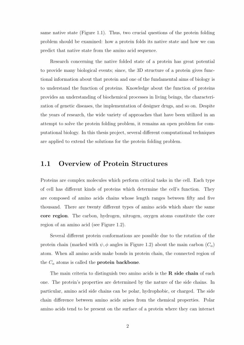
1.2 The structure of two amino acids in a polypeptide chain. Each amino acid
is encircled by a hexagon. The backbone of the protein chain is shown by
a rectangle. . . . . . . . . . . . . . . . . . . . . . . . . . . . . . . . . . 3
1.3 The 3D structure of a protein. The secondary structure elements have
different colors. The α-helix, β-sheet, turn, loop structures are shown in
light blue, red, pink, and grey, respectively. . . . . . . . . . . . . . . . . 5
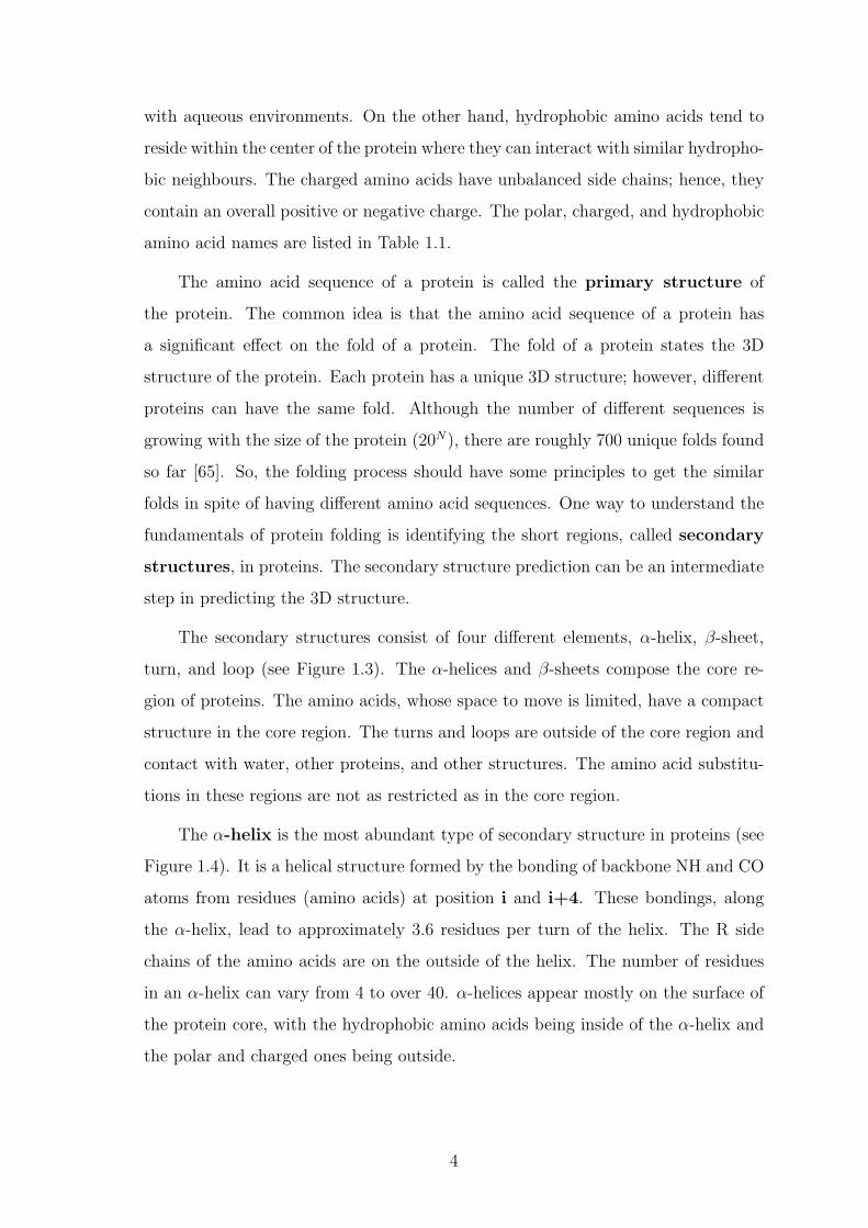
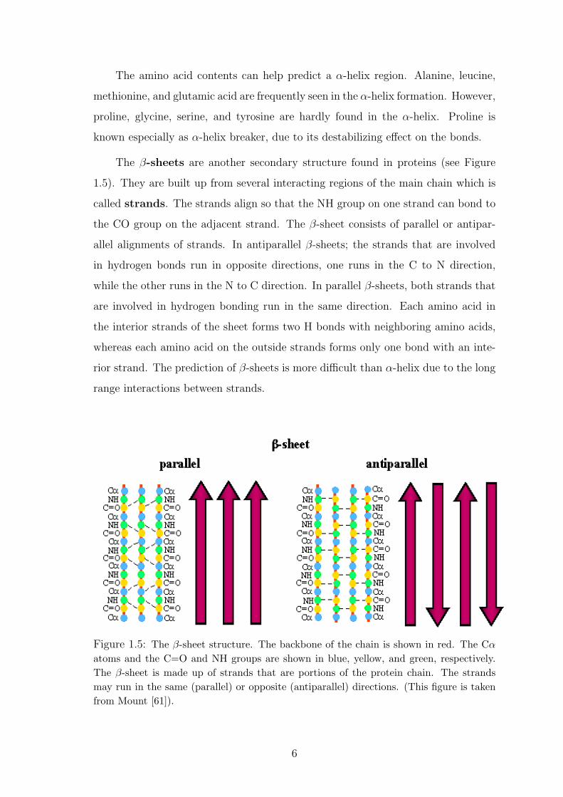
1.4 The α-helix secondary structure. The backbone of the chain is shown
in red. The Cα atoms and the C=O and NH groups are shown in blue,
yellow, and green, respectively. In the α-helix, each C=O group at position
i in the sequence is hydrogen-bonded with the NH group at position i+4.
(This figure is taken from Mount [61]). . . . . . . . . . . . . . . . . . . 5
1.5 The β-sheet structure. The backbone of the chain is shown in red. The
Cα atoms and the C=O and NH groups are shown in blue, yellow, and
green, respectively. The β-sheet is made up of strands that are portions of
the protein chain. The strands may run in the same (parallel) or opposite
(antiparallel) directions. (This figure is taken from Mount [61]). . . . . . 6
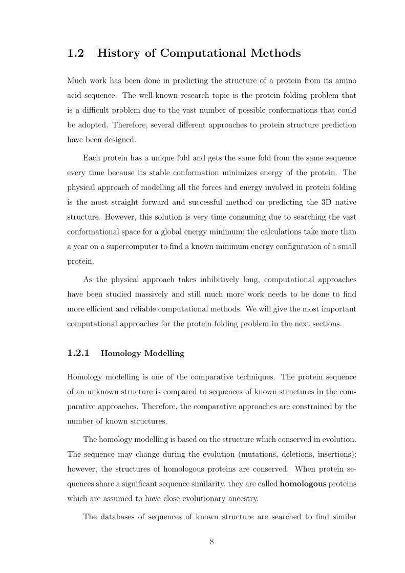
1.6 The γ-turn and β-turn secondary structures. In a γ-turn, a hydrogen bond
exists between residue i (CO) and residue i+2 (NH). In β-turn, a hydrogen
bond exists between residue i (CO) and residue i+3 (NH). . . . . . . . . 7
2.1 The illustration of main four structural classes. . . . . . . . . . . . . . . 14
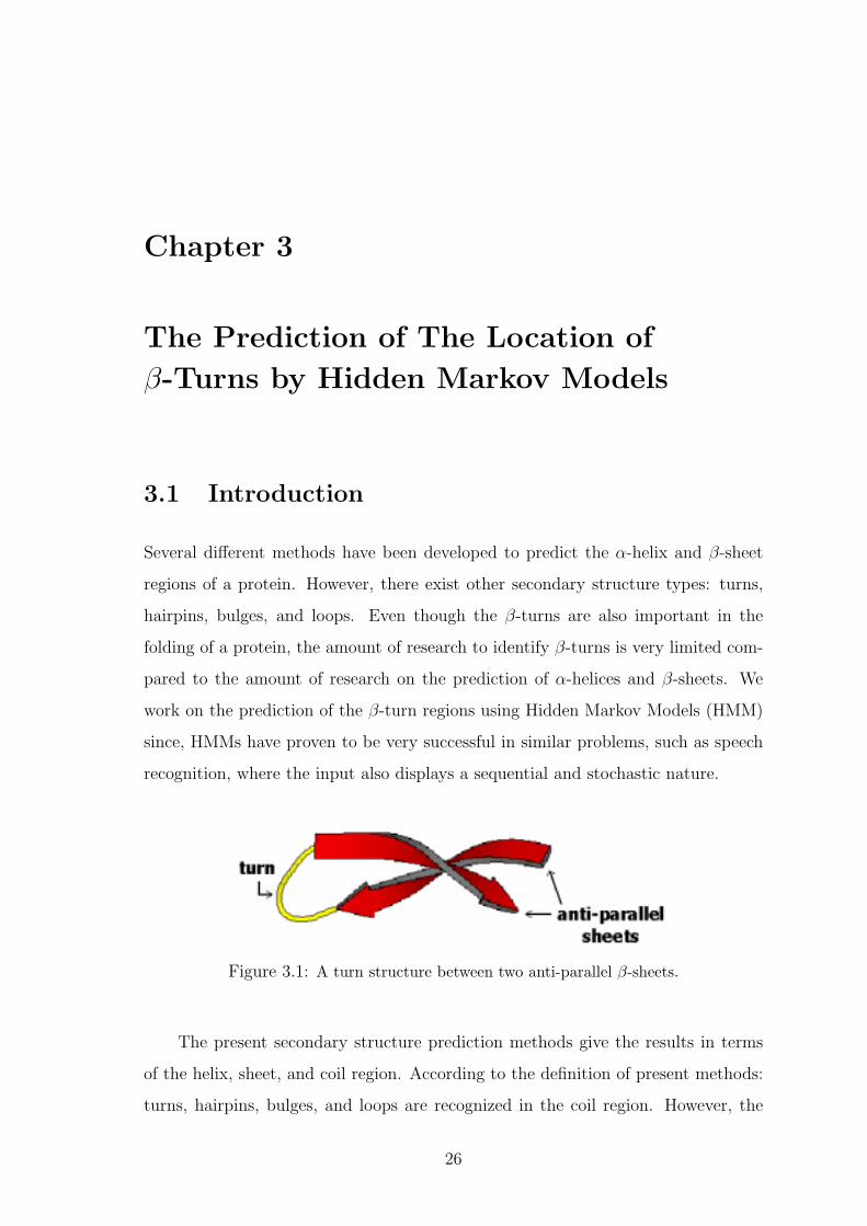
3.1 A turn structure between two anti-parallel β-sheets. . . . . . . . . . . . . 26
xiii
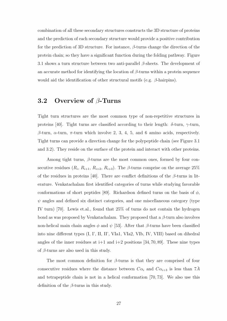
3.2 β-turns consist of four residues which are marked by the blue circles. The
Cα atoms are shown in grey. The hydrogen bond exists between residue i
(CO-red atom) and residue i+3 (NH-blue atom). Two types of β-turns are
very common, type I and type II [49]. Note that the difference between
the angles in the backbone of the second and third residues. This angle is
one criteria to determine type of β-turns. . . . . . . . . . . . . . . . . . 28
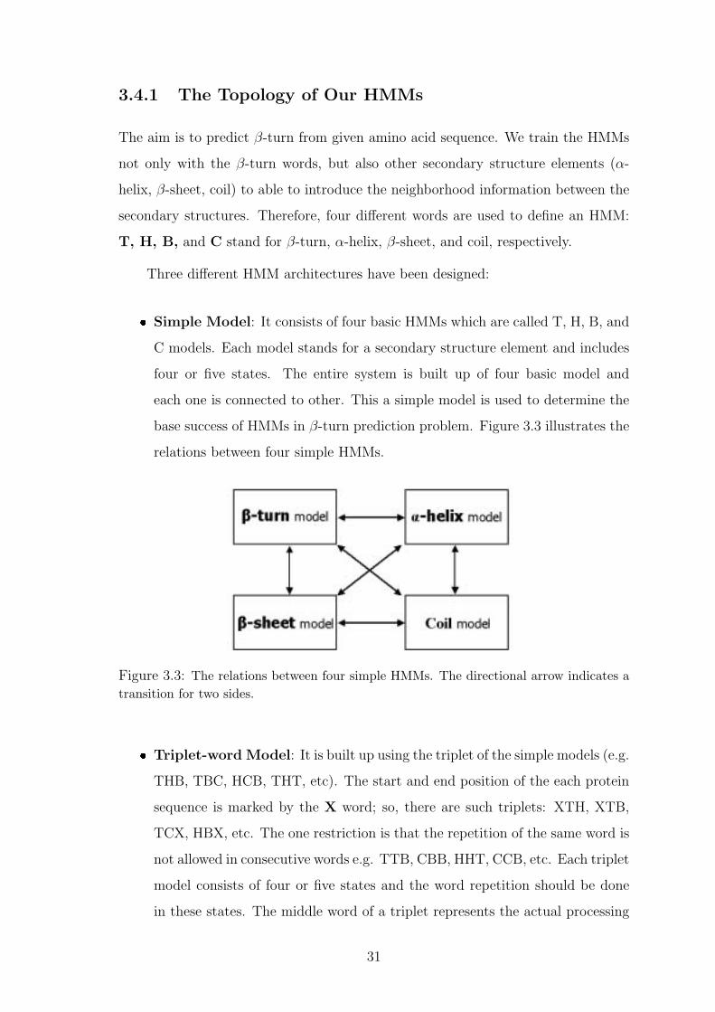
3.3 The relations between four simple HMMs. The directional arrow indicates
a transition for two sides. . . . . . . . . . . . . . . . . . . . . . . . . . 31
3.4 The illustration of constructing steps of a triplet-word model. . . . . . . . 32
3.5 The illustration of constructing steps of a complex model. . . . . . . . . . 33
3.6 Simple left to right HMM with four states. . . . . . . . . . . . . . . . . . 34
3.7 HTK software architecture. . . . . . . . . . . . . . . . . . . . . . . . . . 45
3.8 HTK processing stages. . . . . . . . . . . . . . . . . . . . . . . . . . . . 46
4.1 The illustration of the nine different types of β-turns. The first and fourth
main carbon atoms are marked. The distance between these two atoms is
also given. (The image of each β-turn type is taken from Chou [16].) . . . 54
4.2 The illustration of the process flow in our MLP. . . . . . . . . . . . . . 56
A.1 Data points are mapped into a feature space where they are linearly sep-
arable. . . . . . . . . . . . . . . . . . . . . . . . . . . . . . . . . . . . 66
A.2 Linear separating hyperplanes for the separable case. The support vectors
are H1 and H2. . . . . . . . . . . . . . . . . . . . . . . . . . . . . . . . 67
A.3 Linear separating hyperplanes for the non-separable case. . . . . . . . . . 70
B.1 A Markov chain with states (S1, S2, S3) and state transitions (a11, a23,...). 72
B.2 Illustration of the stages required for the computation of αt+1(j). . . . . . 76
B.3 Illustration of the stages required for the computation of βt(i). . . . . . . 77
C.1 The architecture of one neuron. . . . . . . . . . . . . . . . . . . . . . . 83
C.2 The architecture of 3 layer fully connected MLP. . . . . . . . . . . . . . 84
xiv
List of Tables
1.1 Types of amino acids according to their chemical properties. . . . . . . . 3
2.1 The total number of proteins in each structural class. . . . . . . . . . . . 18
2.2 The content of each amino acid cluster for the 9 cluster case. . . . . . . . 20
2.3 Training performances of Chou [14] versus our results using CCA and
SVM, using the AAC or the Trio AAC. . . . . . . . . . . . . . . . . . . 21
2.4 Test performances of classifiers with training performances shown in Table
2.3. The AAC is applied in both method the CCA and the SVM, in
addition the Trio AAC is used for the SVM. . . . . . . . . . . . . . . . . 22
2.5 Jackknife test performance of the SVM on (117+63) proteins, using the
AAC or the Trio AAC. . . . . . . . . . . . . . . . . . . . . . . . . . . . 23
2.6 Jackknife test performance on 117 proteins (the training set only), as done
by Wang and Yuan (CCA) [92] and our results, obtained by SVM method
using the AAC or the Trio AAC. . . . . . . . . . . . . . . . . . . . . . . 23
3.1 The similarity score of each amino acid in 3D. . . . . . . . . . . . . . . . 36
3.2 The recognition performance of 4 states HMM with different extensions. . 39
3.3 The recognition performance of 60 states HMM with different extensions. . 41
3.4 The recognition performance of 95 states HMM with different extensions. . 42
4.1 The mean dihedral angles for β-turn types. . . . . . . . . . . . . . . . . 53
4.2 The frequency of each β-turn type for the training and test data sets. . . . 57
4.3 The surface area and hydrophobicity features of each amino acid. . . . . . 58
xv
4.4 The correct classification rate of each type of β-turns using the 12D input. 60
4.5 The count of the confused data for the test results in Table 4.4. . . . . . . 61
4.6 The network results using the 12D input vector. The term “Train %”refers
to the ratio of the correctly classified β-turns to the total number of β-
turns in the training set. The term “Test %”refers to the ratio of the
correctly classified β-turns to the total number of β-turns in the test set. . 61
4.7 The correct classification rate of each type of β-turns using the 17D input. 62
4.8 The count of the confused data for the test results in Table 4.7. . . . . . . 62
4.9 The network results using the 17D input vector. . . . . . . . . . . . . . . 62
4.10 The correct classification rate of each type of β-turns using the 18D input. 63
4.11 The count of the confused data for the test results in Table 4.10. . . . . . 63
4.12 The network results using the 18D input vector. . . . . . . . . . . . . . . 64
4.13 The performance comparison of the previous β-turn type classification
works to our method. 1The training performance of Cai et.al. [11]. 2Test
performance of Shepherd et.al. [82]. The ’-’ represents the unreported
result. 3Test performance of our network which is trained by the 17D
input vector. . . . . . . . . . . . . . . . . . . . . . . . . . . . . . . . . 65
C.1 Several different activation functions. . . . . . . . . . . . . . . . . . . . 83
xvi
Chapter 1
Introduction
The past decade has produced many discoveries in the field of biology; particularly,
the completion of the sequencing of the human genome, was a major breakthrough,
which offers a huge sequence of data waiting for processing. There are many applica-
tions for sequence analysis, i.e., gene finding, protein secondary structure prediction,
protein fold prediction, protein function prediction, and interactions of different type
of proteins. Although scientists are trying to find solutions using both experimental
and computational methods, the cost and time limitations inherent in experimen-
tal methods have increased the importance of the development of computational
solutions. Hence, computational biology has a key role to explore in the working
mechanism of the cell machine.
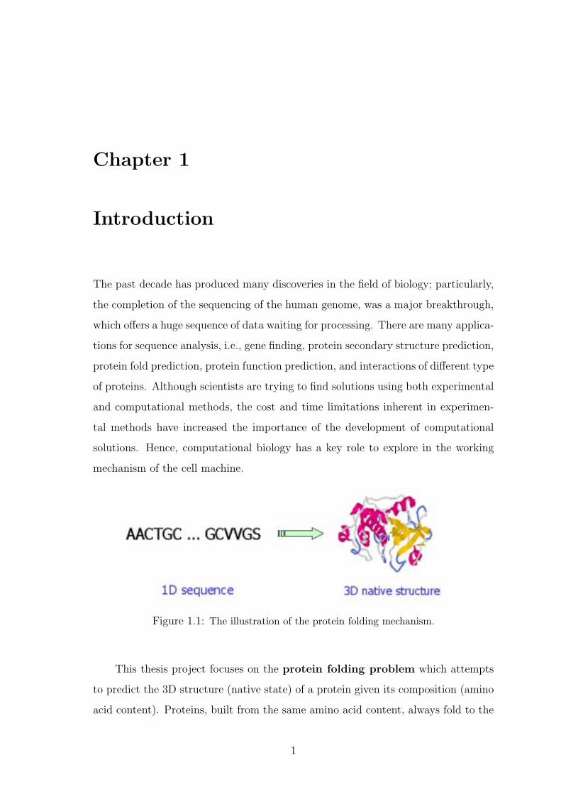
Figure 1.1: The illustration of the protein folding mechanism.
This thesis project focuses on the protein folding problem which attempts
to predict the 3D structure (native state) of a protein given its composition (amino
acid content). Proteins, built from the same amino acid content, always fold to the
1
same native state (Figure 1.1). Thus, two crucial questions of the protein folding
problem should be examined: how a protein folds its native state and how we can
predict that native state from the amino acid sequence.
Research concerning the native folded state of a protein has great potential
to provide many biological events; since, the 3D structure of a protein gives func-
tional information about that protein and one of the fundamental aims of biology is
to understand the function of proteins. Knowledge about the function of proteins
provides an understanding of biochemical processes in living beings, the characteri-
zation of genetic diseases, the implementation of designer drugs, and so on. Despite
the years of research, the wide variety of approaches that have been utilized in an
attempt to solve the protein folding problem, it remains an open problem for com-
putational biology. In this thesis project, several different computational techniques
are applied to extend the solutions for the protein folding problem.
1.1 Overview of Protein Structures
Proteins are complex molecules which perform critical tasks in the cell. Each type
of cell has different kinds of proteins which determine the cell’s function. They
are composed of amino acids chains whose length ranges between fifty and five
thousand. There are twenty different types of amino acids which share the same
core region. The carbon, hydrogen, nitrogen, oxygen atoms constitute the core
region of an amino acid (see Figure 1.2).
Several different protein conformations are possible due to the rotation of the
protein chain (marked with ψ, φ angles in Figure 1.2) about the main carbon (Cα)
atom. When all amino acids make bonds in protein chain, the connected region of
the Cα atoms is called the protein backbone.
The main criteria to distinguish two amino acids is the R side chain of each
one. The protein’s properties are determined by the nature of the side chains. In
particular, amino acid side chains can be polar, hydrophobic, or charged. The side
chain difference between amino acids arises from the chemical properties. Polar
amino acids tend to be present on the surface of a protein where they can interact
2
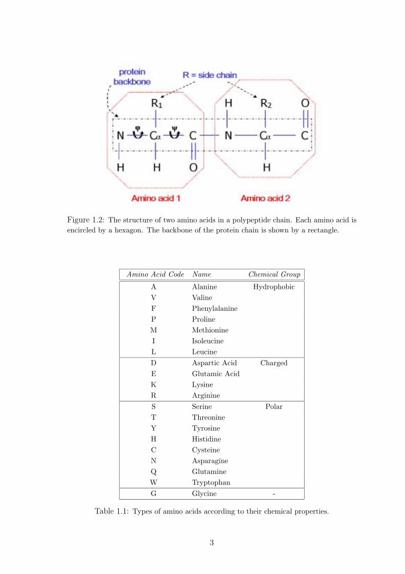
Figure 1.2: The structure of two amino acids in a polypeptide chain. Each amino acid isencircled by a hexagon. The backbone of the protein chain is shown by a rectangle.
Amino Acid Code Name Chemical Group
A Alanine HydrophobicV ValineF PhenylalanineP ProlineM MethionineI IsoleucineL LeucineD Aspartic Acid ChargedE Glutamic AcidK LysineR ArginineS Serine PolarT ThreonineY TyrosineH HistidineC CysteineN AsparagineQ GlutamineW TryptophanG Glycine -
Table 1.1: Types of amino acids according to their chemical properties.
3
with aqueous environments. On the other hand, hydrophobic amino acids tend to
reside within the center of the protein where they can interact with similar hydropho-
bic neighbours. The charged amino acids have unbalanced side chains; hence, they
contain an overall positive or negative charge. The polar, charged, and hydrophobic
amino acid names are listed in Table 1.1.
The amino acid sequence of a protein is called the primary structure of
the protein. The common idea is that the amino acid sequence of a protein has
a significant effect on the fold of a protein. The fold of a protein states the 3D
structure of the protein. Each protein has a unique 3D structure; however, different
proteins can have the same fold. Although the number of different sequences is
growing with the size of the protein (20N), there are roughly 700 unique folds found
so far [65]. So, the folding process should have some principles to get the similar
folds in spite of having different amino acid sequences. One way to understand the
fundamentals of protein folding is identifying the short regions, called secondary
structures, in proteins. The secondary structure prediction can be an intermediate
step in predicting the 3D structure.
The secondary structures consist of four different elements, α-helix, β-sheet,
turn, and loop (see Figure 1.3). The α-helices and β-sheets compose the core re-
gion of proteins. The amino acids, whose space to move is limited, have a compact
structure in the core region. The turns and loops are outside of the core region and
contact with water, other proteins, and other structures. The amino acid substitu-
tions in these regions are not as restricted as in the core region.
The α-helix is the most abundant type of secondary structure in proteins (see
Figure 1.4). It is a helical structure formed by the bonding of backbone NH and CO
atoms from residues (amino acids) at position i and i+4. These bondings, along
the α-helix, lead to approximately 3.6 residues per turn of the helix. The R side
chains of the amino acids are on the outside of the helix. The number of residues
in an α-helix can vary from 4 to over 40. α-helices appear mostly on the surface of
the protein core, with the hydrophobic amino acids being inside of the α-helix and
the polar and charged ones being outside.
4
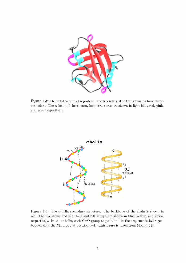
Figure 1.3: The 3D structure of a protein. The secondary structure elements have differ-ent colors. The α-helix, β-sheet, turn, loop structures are shown in light blue, red, pink,and grey, respectively.
Figure 1.4: The α-helix secondary structure. The backbone of the chain is shown inred. The Cα atoms and the C=O and NH groups are shown in blue, yellow, and green,respectively. In the α-helix, each C=O group at position i in the sequence is hydrogen-bonded with the NH group at position i+4. (This figure is taken from Mount [61]).
5
The amino acid contents can help predict a α-helix region. Alanine, leucine,
methionine, and glutamic acid are frequently seen in the α-helix formation. However,
proline, glycine, serine, and tyrosine are hardly found in the α-helix. Proline is
known especially as α-helix breaker, due to its destabilizing effect on the bonds.
The β-sheets are another secondary structure found in proteins (see Figure
1.5). They are built up from several interacting regions of the main chain which is
called strands. The strands align so that the NH group on one strand can bond to
the CO group on the adjacent strand. The β-sheet consists of parallel or antipar-
allel alignments of strands. In antiparallel β-sheets; the strands that are involved
in hydrogen bonds run in opposite directions, one runs in the C to N direction,
while the other runs in the N to C direction. In parallel β-sheets, both strands that
are involved in hydrogen bonding run in the same direction. Each amino acid in
the interior strands of the sheet forms two H bonds with neighboring amino acids,
whereas each amino acid on the outside strands forms only one bond with an inte-
rior strand. The prediction of β-sheets is more difficult than α-helix due to the long
range interactions between strands.
Figure 1.5: The β-sheet structure. The backbone of the chain is shown in red. The Cα
atoms and the C=O and NH groups are shown in blue, yellow, and green, respectively.The β-sheet is made up of strands that are portions of the protein chain. The strandsmay run in the same (parallel) or opposite (antiparallel) directions. (This figure is takenfrom Mount [61]).
6
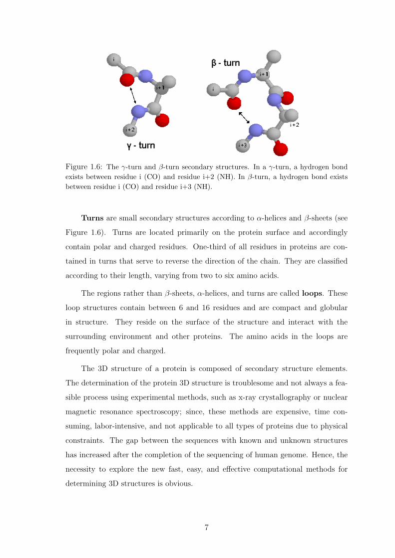
Figure 1.6: The γ-turn and β-turn secondary structures. In a γ-turn, a hydrogen bondexists between residue i (CO) and residue i+2 (NH). In β-turn, a hydrogen bond existsbetween residue i (CO) and residue i+3 (NH).
Turns are small secondary structures according to α-helices and β-sheets (see
Figure 1.6). Turns are located primarily on the protein surface and accordingly
contain polar and charged residues. One-third of all residues in proteins are con-
tained in turns that serve to reverse the direction of the chain. They are classified
according to their length, varying from two to six amino acids.
The regions rather than β-sheets, α-helices, and turns are called loops. These
loop structures contain between 6 and 16 residues and are compact and globular
in structure. They reside on the surface of the structure and interact with the
surrounding environment and other proteins. The amino acids in the loops are
frequently polar and charged.
The 3D structure of a protein is composed of secondary structure elements.
The determination of the protein 3D structure is troublesome and not always a fea-
sible process using experimental methods, such as x-ray crystallography or nuclear
magnetic resonance spectroscopy; since, these methods are expensive, time con-
suming, labor-intensive, and not applicable to all types of proteins due to physical
constraints. The gap between the sequences with known and unknown structures
has increased after the completion of the sequencing of human genome. Hence, the
necessity to explore the new fast, easy, and effective computational methods for
determining 3D structures is obvious.
7
1.2 History of Computational Methods
Much work has been done in predicting the structure of a protein from its amino
acid sequence. The well-known research topic is the protein folding problem that
is a difficult problem due to the vast number of possible conformations that could
be adopted. Therefore, several different approaches to protein structure prediction
have been designed.
Each protein has a unique fold and gets the same fold from the same sequence
every time because its stable conformation minimizes energy of the protein. The
physical approach of modelling all the forces and energy involved in protein folding
is the most straight forward and successful method on predicting the 3D native
structure. However, this solution is very time consuming due to searching the vast
conformational space for a global energy minimum; the calculations take more than
a year on a supercomputer to find a known minimum energy configuration of a small
protein.
As the physical approach takes inhibitively long, computational approaches
have been studied massively and still much more work needs to be done to find
more efficient and reliable computational methods. We will give the most important
computational approaches for the protein folding problem in the next sections.
1.2.1 Homology Modelling
Homology modelling is one of the comparative techniques. The protein sequence
of an unknown structure is compared to sequences of known structures in the com-
parative approaches. Therefore, the comparative approaches are constrained by the
number of known structures.
The homology modelling is based on the structure which conserved in evolution.
The sequence may change during the evolution (mutations, deletions, insertions);
however, the structures of homologous proteins are conserved. When protein se-
quences share a significant sequence similarity, they are called homologous proteins
which are assumed to have close evolutionary ancestry.
The databases of sequences of known structure are searched to find similar
8
(homologous) sequences. The alignment of the homologous sequences is used as
input for the homology modelling program. It uses the alignment of proteins to
generate spatial constraints (distance between non-adjacent residues, the dihedral
angles between adjacent residues, and so on) on the target sequence. Finally, the
homology modeler generates a possible conformation of the protein and optimises it
with respect to the spatial constraints.
The most commonly used homology modelling programs are the Modeler and
WHAT IF [56,91].
1.2.2 Threading
Threading attempts to find a known fold that the given sequence with unknown
structure could construct. Sometimes threading is called fold recognition.
The steps of measuring the best fitted fold in the whole fold space can be
summarized in the following: Firstly, the target sequence (with an unknown fold) is
threaded through all the existing folds. Then, a score function should be assigned to
make a comparison between all threaded folds. The contact potential and sequence
profile method are the most common techniques to compute the score function.
After that, a search strategy for the threading should be determined. There exist
many local minimas in the search space; hence, the search algorithm is a crucial
part of the threading. There are several different heuristics to search the whole
fold space, i.e., double dynamic programming [37], Gibbs sampling algorithm [7],
branch and bound algorithm [48], recursive dynamic programming [86], and neural
network [38].
The most successful threading servers are GenThreader and Fugue [38,83].
1.2.3 Secondary Structure Prediction
The detection of the secondary structures of a protein would give useful information
to determine the 3D structure of that protein. Therefore, the prediction of the sec-
ondary structures of proteins can be one subgoal within the protein folding problem.
There exist multiple generations of approaches to predict the secondary structures
9
of proteins. These approaches are explained below in detail; since the secondary
structure prediction closely relates to the subtopics of this thesis.
The first generation of the secondary structure prediction approaches used the
single amino acid compositions [6, 66, 84]. In other words, these approaches used
the percentage of each amino acid in a given protein (e.g. %7 alanine, %3 proline,
%6 cystine). Due to the small size of the known structure databases, the statistical
results of these approaches were not realistic.
Along with increasing the size of the known structure databases, a second gen-
eration of prediction methods were developed. They computed the amino acid
compositions for the longer segments to incorporate the neighboring information of
amino acids. The scientists applied several different machine learning techniques
to analyse the segments with long length. The multi layer neural networks were
the most popular machine learning technique [31,46,54,68]. The prediction perfor-
mance of these methods was lower than 70% ; furthermore, they could not predict
β-strands better than could random prediction. The reason for the limited prediction
performance was that the training systems by using merely the local information;
however, long range amino acid interactions have effects on the formation of the
secondary structures like β-strands. If the long range effects had been included to
the next generation of secondary structure prediction methods, would have played
more important role in determining the 3D structure of proteins.
The third generation secondary structure prediction approaches have tried to
combine machine learning techniques and evolutionary information. The sequence
of a protein may change while the evolution but its structure is preserved. The
different alignment techniques have been applied to consider the evolutionary in-
formation between proteins. The first usage of alignment information has been
proposed first by Maxfield and Scheraga and by Zvelebil et al. [57, 96]. In the se-
quence alignment, two or more strings (amino acid segments) are aligned together in
order to get the highest number of matching characters. Gaps may be inserted into
a string in order to shift the remaining characters into better matches. The above
research compiled predictions for each protein in an alignment, then averaged over
all proteins. Profiles which are compiled from the multiple sequence alignments
10
are the better way of considering evolutionary information [57,74]. Several methods
have performed close prediction accuracies by using neural network based methods
and profile scores [23,27,44,59,72,75,79].
A new alignment search method has been introduced which automatically
aligns protein families based on profiles. Several research groups have developed
the profile-based databases searches [25, 29, 33, 42, 51, 64, 85]. The development of
PSI-BLAST and Hidden Markov Models have been increased the prediction perfor-
mances [1, 41]. David Jones pioneered the use of the iterated PSI-BLAST searches
on large databases automatically. He has developed the PSIPRED secondary struc-
ture method using that PSI-BLAST searches results [39]. Kevin Karplus et al. have
proposed their own method (SAM-T99sec) which finds the diverged profiles using
Hidden Markov Models [42]. Cuff and Barton also used PSI-BLAST alignments for
JPred2 [21]. SSpro used a different architecture which was an advanced recursive
neural network system [3]. This method has tried to solve the problem of predicting
too short segments by using the recursive neural network and multiple alignments.
The current state of the art for the secondary structure prediction is near
78% for three state per residue accuracy (the percentage of α-helices, β-sheets, and
coils). The methods PROF, PSIPRED, and SSpro perform the most accurate per-
formances, according to EVA results, an automatic server evaluating the automatic
prediction servers [3,39,76,77]. EVA takes the newest experimental structures added
to PDB, sends the sequences to all prediction servers, and collects the results [5].
The existing methods improve the prediction of the α-helix and β-strand sec-
ondary structure elements. There exist small stable structures such as turns, hairpin
loops. However, the prediction of these structures is not so easy and the research in
this area are not satisfactory.
After this short review of the secondary structure prediction methods, we want
to mention about the scope of the thesis. We have worked on the small secondary
structures, β-turns, which have a critical role on the folding of protein. The for-
mation of these turns has been thought to be an important early step in the protein
folding pathway. The identification of β-turns would provide important advance-
ments for the protein folding pathway; since, β-turns are commonly found to link
11
two strands of anti-parallel beta-sheet. We have developed Hidden Markov Mod-
els to identify the location of β-turns in a given protein sequence. Type of β-turns
has been also identified by Artificial Neural Networks.
Some third generation structure prediction approaches have tried to improve
the accuracy of assigning the secondary structural class (all-α, all-β, α/β, other). In
another part of the thesis, we have applied Support Vector Machines to improve
the classification accuracy of the secondary structural class of proteins.
1.3 Organization of The Thesis
In Chapter 2, we present our work for the classification of the protein structural
classes by Support Vector Machines. In Chapter 3, the work on predicting of the
location of β-turns by Hidden Markov Models is presented. Finally in Chapter 4,
we present the classification of type of β-turns by Artificial Neural Networks.
12
Chapter 2
Protein Structural Class Determination
Using Support Vector Machines
2.1 Introduction
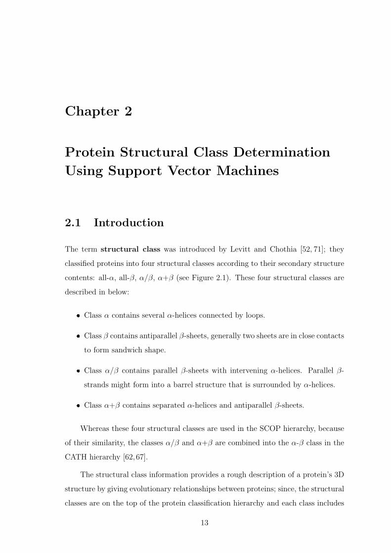
The term structural class was introduced by Levitt and Chothia [52, 71]; they
classified proteins into four structural classes according to their secondary structure
contents: all-α, all-β, α/β, α+β (see Figure 2.1). These four structural classes are
described in below:
� Class α contains several α-helices connected by loops.
� Class β contains antiparallel β-sheets, generally two sheets are in close contacts
to form sandwich shape.
� Class α/β contains parallel β-sheets with intervening α-helices. Parallel β-
strands might form into a barrel structure that is surrounded by α-helices.
� Class α+β contains separated α-helices and antiparallel β-sheets.
Whereas these four structural classes are used in the SCOP hierarchy, because
of their similarity, the classes α/β and α+β are combined into the α-β class in the
CATH hierarchy [62,67].
The structural class information provides a rough description of a protein’s 3D
structure by giving evolutionary relationships between proteins; since, the structural
classes are on the top of the protein classification hierarchy and each class includes
13
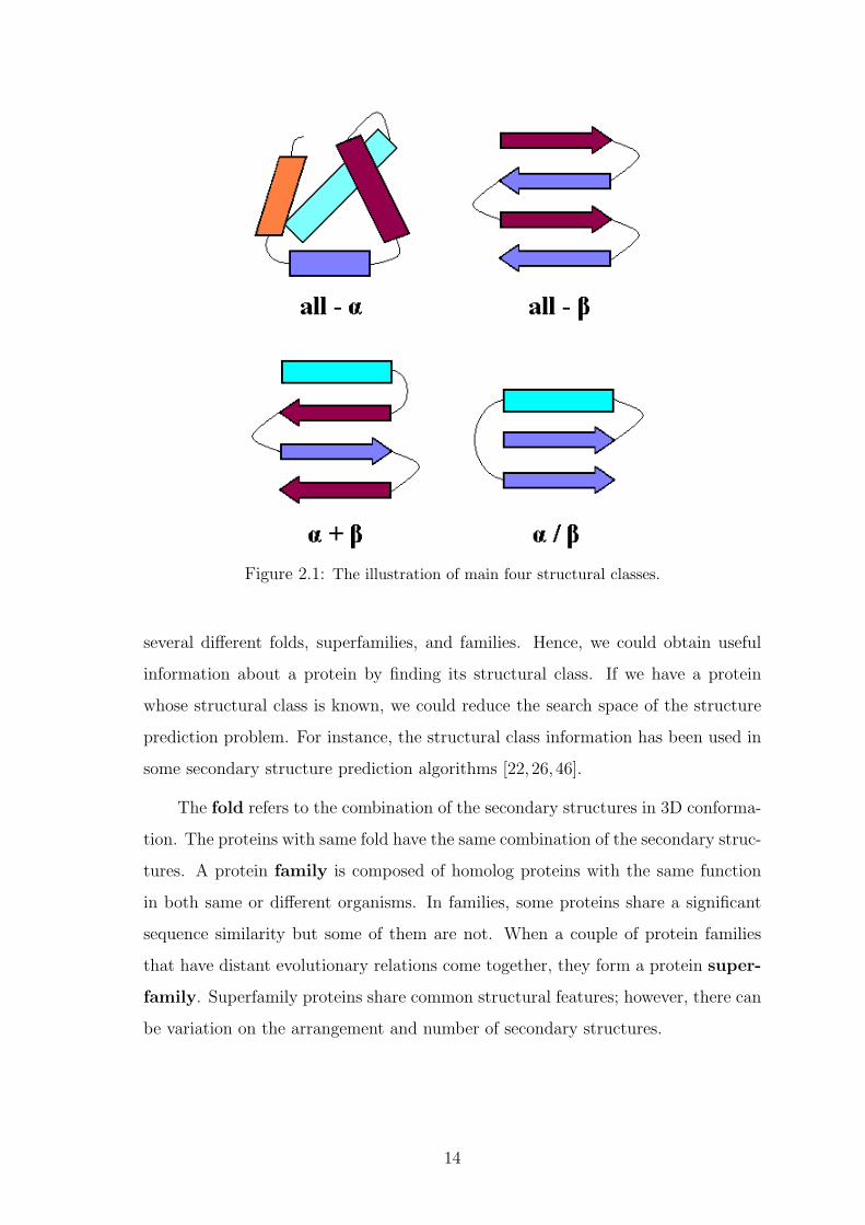
Figure 2.1: The illustration of main four structural classes.
several different folds, superfamilies, and families. Hence, we could obtain useful
information about a protein by finding its structural class. If we have a protein
whose structural class is known, we could reduce the search space of the structure
prediction problem. For instance, the structural class information has been used in
some secondary structure prediction algorithms [22,26,46].
The fold refers to the combination of the secondary structures in 3D conforma-
tion. The proteins with same fold have the same combination of the secondary struc-
tures. A protein family is composed of homolog proteins with the same function
in both same or different organisms. In families, some proteins share a significant
sequence similarity but some of them are not. When a couple of protein families
that have distant evolutionary relations come together, they form a protein super-
family. Superfamily proteins share common structural features; however, there can
be variation on the arrangement and number of secondary structures.
14
2.2 Previous Work
During the past ten years, many scientists worked on the structural classification
problem [2,9,10,12,14,17,19,24,45,60,63,95]. The classification methods are various:
the Component Coupled Algorithm (CCA), Artificial Neural Networks, Support
Vector Machines (SVM) etc. However, they typically use the simple feature of
amino acid composition of the protein as the base for the classification.
Among these structural classification studies, an independently developed work
uses a SVM as the classification tool and the amino acid composition [10]. Although
their data set is completely different, the classification tool and feature is similar
with our method. Their average classification performance in the Jackknife test is
93.2%, for 204 protein domains.
Another method, the CCA, also using the amino acid composition, had reported
very successful results for the same problem. So, we wanted to duplicate and improve
this work, in our study. The details of the CCA is explained in the following section.
2.2.1 Component Coupled Algorithm
K.C. Chou used what they called the Component Coupled Algorithm to assign
a protein into one of the four structural classes [14]. The CCA is more sophisti-
cated from the earlier techniques since, it uses the Mahalanobis distance [55] as its
discriminant function, taking into effect the covariance of amino acid compositions
(coupling), in addition to only considering the mean amino acid composition vectors
of structural classes for the classification. The brief summary of CCA is given below:
The Amino Acid Composition (AAC) represents protein with a 20 dimen-
sional vector corresponding to the composition (frequency of occurrence) of the 20
amino acids in the protein. Since, the frequencies sum up to 1, only 19 out of 20 are
independent and the AAC can be represented in 19 independent dimensions. The
AAC vector of a protein is:
15
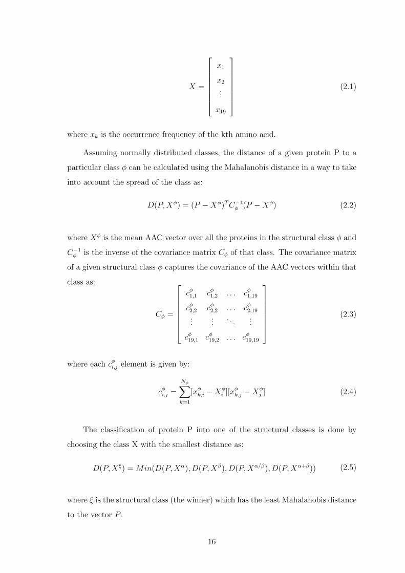
X =
x1
x2
...
x19
(2.1)
where xk is the occurrence frequency of the kth amino acid.
Assuming normally distributed classes, the distance of a given protein P to a
particular class φ can be calculated using the Mahalanobis distance in a way to take
into account the spread of the class as:
D(P,Xφ) = (P − Xφ)T C−1φ (P − Xφ) (2.2)
where Xφ is the mean AAC vector over all the proteins in the structural class φ and
C−1φ is the inverse of the covariance matrix Cφ of that class. The covariance matrix
of a given structural class φ captures the covariance of the AAC vectors within that
class as:
Cφ =
cφ1,1 cφ
1,2 . . . cφ1,19
cφ2,2 cφ
2,2 . . . cφ2,19
......
. . ....
cφ19,1 cφ
19,2 . . . cφ19,19
(2.3)
where each cφi,j element is given by:
cφi,j =
Nφ∑k=1
[xφk,i − Xφ
i ][xφk,j − Xφ
j ] (2.4)
The classification of protein P into one of the structural classes is done by
choosing the class X with the smallest distance as:
D(P,Xξ) = Min(D(P,Xα), D(P,Xβ), D(P,Xα/β), D(P,Xα+β)) (2.5)
where ξ is the structural class (the winner) which has the least Mahalanobis distance
to the vector P .
16
2.3 Our Method
Although the AAC largely determines structural class, its capacity is limited, since
one looses information by representing a protein with only a 20 dimensional vector.
Therefore, we try to improve the classification capacity of the AAC by extending it
to the Trio Amino Acid Composition (Trio AAC). The Trio AAC is calculated
from the occurrence frequencies of consecutive amino acid triplets in a protein.
The frequency distribution of neighboring triplets is very sparse because of the
high dimensionality of the Trio AAC input vector (203). Furthermore, one also has to
take into account the evolutionary information which shows that certain amino acids
can be replaced by the others without disrupting the function of a protein. These
replacements generally occur between amino acids which have similar physical and
chemical properties. Hence, several different clustering of the amino acids which take
into account these similarities and reduce the dimensionality, have been used [87].
In this thesis, the performance of SVMs and the CCA using the AAC feature
(described in the previous Section 2.2.1), are compared to observe their classification
capability. The CCA is applied on the same data set to classify the protein using the
Mahalanobis distance between its AAC vector and each structural class. Both the
AAC and the Trio AAC features have been used on SVMs. The detailed explanation
of the construction of the feature sets will be given in Section 2.3.3.
2.3.1 Support Vector Machine
SVM (see Appendix A) is a supervised machine learning technique which seeks an
optimal discrimination of two classes, in high dimensional feature space. The supe-
rior generalization power, especially for high dimensional data, and fast convergence
during training are the main advantages of SVMs. We also preferred to use SVMs
as the classification tool because of its high classification performance on the pro-
tein structural classification problem [10, 24, 88]. The LIBSVM software have been
applied in predicting the structural classes [13].
Generally, SVMs are designed for 2-class classification problems whereas our
work requires a multi-class classification. Multi-class classification is typically solved
17
using voting schemes based on combining binary classification decision functions. In
the LIBSVM tool that we have used, the one-against-one approach is used. In
this scheme, k(k − 1)/2 classifiers are constructed for k class, each one trained with
data from only two different classes. To obtain the multi-class label for a given
data point, each of these classifiers makes its decision and the class label with the
maximum number of votes overall is designated as the correct label of a data point.
In order to get good classification results the parameters of SVM, especially
the kernel type and the error-margin tradeoff (C), should be fixed. The Gaussian
kernels are used since they typically provide better linear separation compared to
Polynomial and Sigmoid kernels. The value of the parameter C was fixed during
the training and later used during the testing. The best performance was obtained
with C values ranging from 10 to 100 in various tasks.
2.3.2 Data Set
We have used the same data set with Chou to make the comparison between the
performances of classification methods [14]. Data set consist of 117 training proteins
and 63 test proteins. Since we could not find the PDB files of 4 proteins (1CTC,
1LIG, 1PRF in training set; 1PDE in test set) included in their database, we used
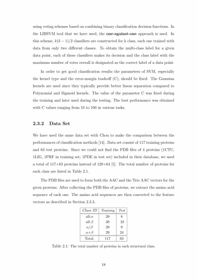
a total of 117+63 proteins instead of 120+64 [5]. The total number of proteins for
each class are listed in Table 2.1.
The PDB files are used to form both the AAC and the Trio AAC vectors for the
given proteins. After collecting the PDB files of proteins, we extract the amino acid
sequence of each one. The amino acid sequences are then converted to the feature
vectors as described in Section 2.3.3.
Class ID Training Test
all-α 29 8all-β 30 22α/β 29 9α+β 29 24
Total: 117 63
Table 2.1: The total number of proteins in each structural class.
18
There are several strategies to classify a protein into one of the structural classes.
It is commonly based on the percentage of α-helix and β-sheet residues in the
protein. K.C. Chou also uses the same method to classify proteins in the data set.
The percentage of α-helix and β-sheet residues for each class is explained below:
� All-α : α-helix > 40% and β-sheet < 5%
� All-β : α-helix < 5% and β-sheet > 40%
� α/β : α-helix > 15% and β-sheet > 15% and more than 60% parallel β-sheets
� α+β : α-helix > 15% and β-sheet > 15% and more than 60% antiparallel
β-sheets
2.3.3 Feature Sets
The training and test data obtained from the PDB are used to form feature sets.
The amino acid sequences are converted to the feature vectors as explained below.
AAC
The AAC represents protein with a 20 dimensional vector corresponding to the
composition (frequency of occurrence) of the 20 amino acids in the protein. The
AAC can be used as a 19 dimensional vector since the frequencies sum up to 1,
only 19 out of 20 amino acids are independent; hence, only 19 dimensions of the
AAC vector is used as input. The details of constructing AAC vector was given in
previous Section 2.2.1.
Trio AAC
The Trio AAC is the occurrence frequency of all possible consecutive triplets of
amino acids, or amino acid clusters, in the protein. Whereas the AAC is a 20-
dimensional vector, the neighborhood composition of triplets of amino acids requires
a 20x20x20 (8000) dimensional vector (e.g. AAA, AAC, ...). We reduce the dimen-
sionality of the Trio AAC input vector using various different clusterings of the
amino acids, also taking into account the evolutionary information.
19
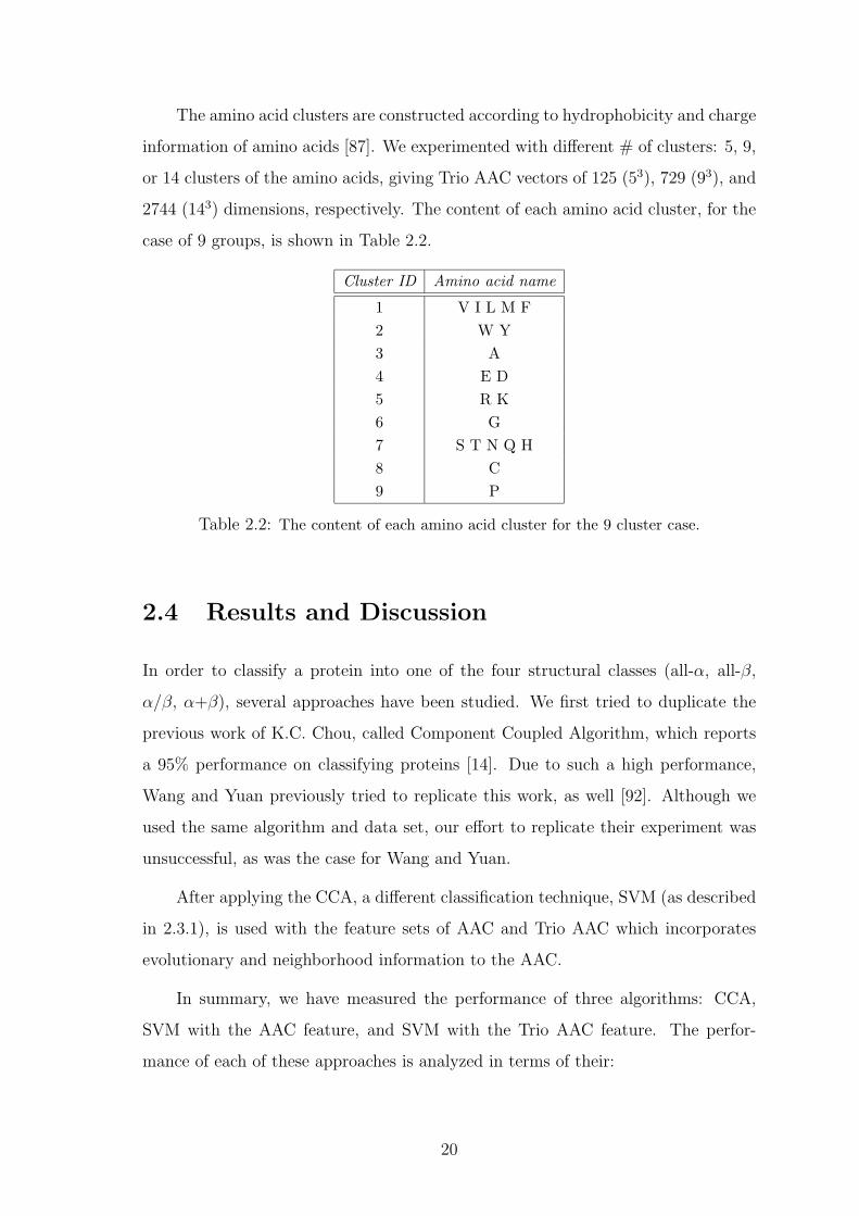
The amino acid clusters are constructed according to hydrophobicity and charge
information of amino acids [87]. We experimented with different # of clusters: 5, 9,
or 14 clusters of the amino acids, giving Trio AAC vectors of 125 (53), 729 (93), and
2744 (143) dimensions, respectively. The content of each amino acid cluster, for the
case of 9 groups, is shown in Table 2.2.
Cluster ID Amino acid name
1 V I L M F2 W Y3 A4 E D5 R K6 G7 S T N Q H8 C9 P
Table 2.2: The content of each amino acid cluster for the 9 cluster case.
2.4 Results and Discussion
In order to classify a protein into one of the four structural classes (all-α, all-β,
α/β, α+β), several approaches have been studied. We first tried to duplicate the
previous work of K.C. Chou, called Component Coupled Algorithm, which reports
a 95% performance on classifying proteins [14]. Due to such a high performance,
Wang and Yuan previously tried to replicate this work, as well [92]. Although we
used the same algorithm and data set, our effort to replicate their experiment was
unsuccessful, as was the case for Wang and Yuan.
After applying the CCA, a different classification technique, SVM (as described
in 2.3.1), is used with the feature sets of AAC and Trio AAC which incorporates
evolutionary and neighborhood information to the AAC.
In summary, we have measured the performance of three algorithms: CCA,
SVM with the AAC feature, and SVM with the Trio AAC feature. The perfor-
mance of each of these approaches is analyzed in terms of their:
20
� performance of learning the training data (train and test with training data)
� generalization performance on test data (train with training data, test with
test data)
� generalization performance using cross-validation techniques (train with all
data, test with the one left out)
2.4.1 Training Performance
The term training performance is used to denote the level of learning after train-
ing; previously the term self-consistency was used to refer to the same concept.
Specifically, the training performance is the percentage of the correctly classified
training data, once the training completes. Hence, it is an indication of how well
the training data is learned. Even though, the performance result on the test set is
the relevant factor, as it indicates the success on unseen data, the training perfor-
mance is also useful because it indicates how well the problem is learnt using the
particular classification method.
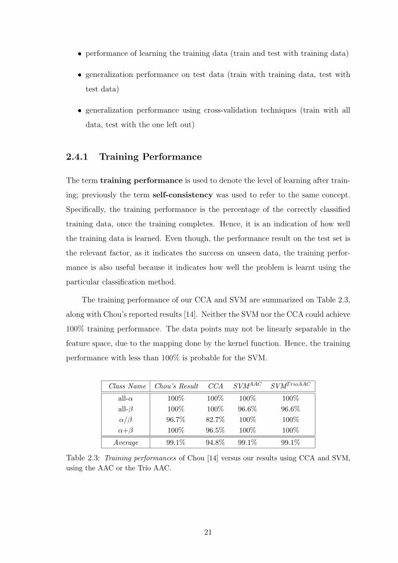
The training performance of our CCA and SVM are summarized on Table 2.3,
along with Chou’s reported results [14]. Neither the SVM nor the CCA could achieve
100% training performance. The data points may not be linearly separable in the
feature space, due to the mapping done by the kernel function. Hence, the training
performance with less than 100% is probable for the SVM.
Class Name Chou’s Result CCA SVMAAC SVMTrioAAC
all-α 100% 100% 100% 100%all-β 100% 100% 96.6% 96.6%α/β 96.7% 82.7% 100% 100%α+β 100% 96.5% 100% 100%
Average 99.1% 94.8% 99.1% 99.1%
Table 2.3: Training performances of Chou [14] versus our results using CCA and SVM,using the AAC or the Trio AAC.
21
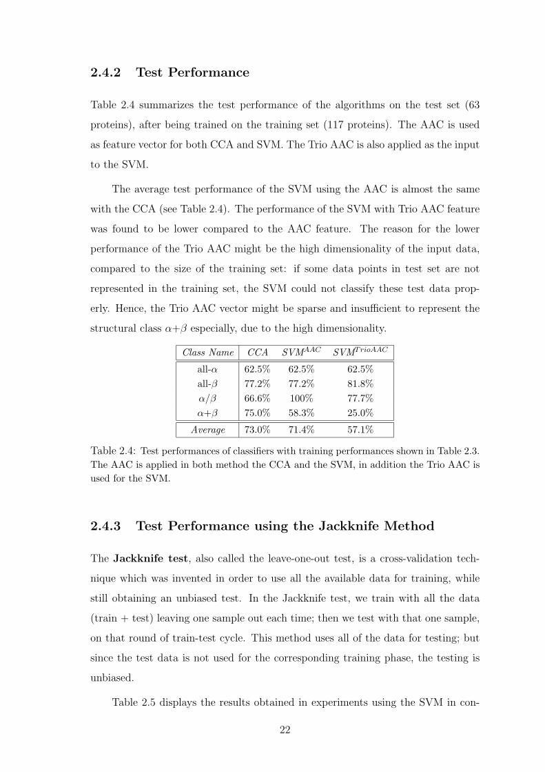
2.4.2 Test Performance
Table 2.4 summarizes the test performance of the algorithms on the test set (63
proteins), after being trained on the training set (117 proteins). The AAC is used
as feature vector for both CCA and SVM. The Trio AAC is also applied as the input
to the SVM.
The average test performance of the SVM using the AAC is almost the same
with the CCA (see Table 2.4). The performance of the SVM with Trio AAC feature
was found to be lower compared to the AAC feature. The reason for the lower
performance of the Trio AAC might be the high dimensionality of the input data,
compared to the size of the training set: if some data points in test set are not
represented in the training set, the SVM could not classify these test data prop-
erly. Hence, the Trio AAC vector might be sparse and insufficient to represent the
structural class α+β especially, due to the high dimensionality.
Class Name CCA SVMAAC SVMTrioAAC
all-α 62.5% 62.5% 62.5%all-β 77.2% 77.2% 81.8%α/β 66.6% 100% 77.7%α+β 75.0% 58.3% 25.0%
Average 73.0% 71.4% 57.1%
Table 2.4: Test performances of classifiers with training performances shown in Table 2.3.The AAC is applied in both method the CCA and the SVM, in addition the Trio AAC isused for the SVM.
2.4.3 Test Performance using the Jackknife Method
The Jackknife test, also called the leave-one-out test, is a cross-validation tech-
nique which was invented in order to use all the available data for training, while
still obtaining an unbiased test. In the Jackknife test, we train with all the data
(train + test) leaving one sample out each time; then we test with that one sample,
on that round of train-test cycle. This method uses all of the data for testing; but
since the test data is not used for the corresponding training phase, the testing is
unbiased.
Table 2.5 displays the results obtained in experiments using the SVM in con-
22
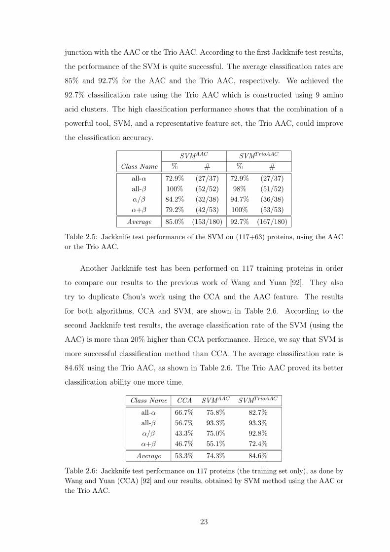
junction with the AAC or the Trio AAC. According to the first Jackknife test results,
the performance of the SVM is quite successful. The average classification rates are
85% and 92.7% for the AAC and the Trio AAC, respectively. We achieved the
92.7% classification rate using the Trio AAC which is constructed using 9 amino
acid clusters. The high classification performance shows that the combination of a
powerful tool, SVM, and a representative feature set, the Trio AAC, could improve
the classification accuracy.
SVMAAC SVMTrioAAC
Class Name % # % #
all-α 72.9% (27/37) 72.9% (27/37)all-β 100% (52/52) 98% (51/52)α/β 84.2% (32/38) 94.7% (36/38)α+β 79.2% (42/53) 100% (53/53)
Average 85.0% (153/180) 92.7% (167/180)
Table 2.5: Jackknife test performance of the SVM on (117+63) proteins, using the AACor the Trio AAC.
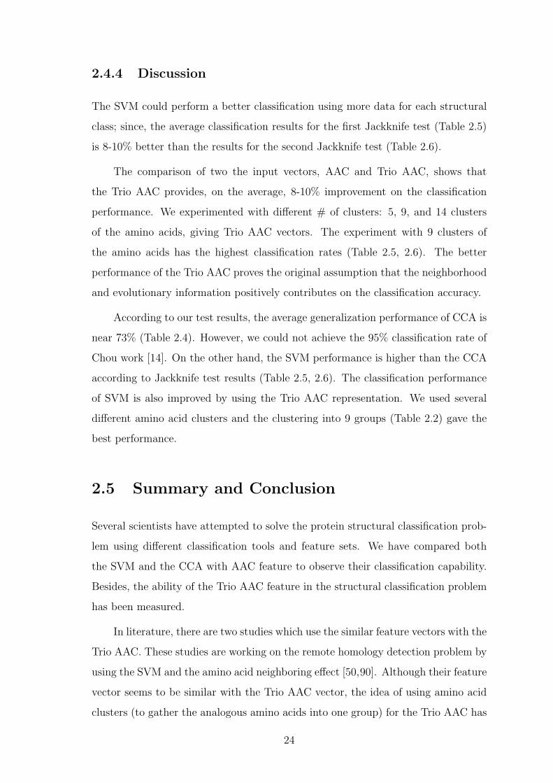
Another Jackknife test has been performed on 117 training proteins in order
to compare our results to the previous work of Wang and Yuan [92]. They also
try to duplicate Chou’s work using the CCA and the AAC feature. The results
for both algorithms, CCA and SVM, are shown in Table 2.6. According to the
second Jackknife test results, the average classification rate of the SVM (using the
AAC) is more than 20% higher than CCA performance. Hence, we say that SVM is
more successful classification method than CCA. The average classification rate is
84.6% using the Trio AAC, as shown in Table 2.6. The Trio AAC proved its better
classification ability one more time.
Class Name CCA SVMAAC SVMTrioAAC
all-α 66.7% 75.8% 82.7%all-β 56.7% 93.3% 93.3%α/β 43.3% 75.0% 92.8%α+β 46.7% 55.1% 72.4%
Average 53.3% 74.3% 84.6%
Table 2.6: Jackknife test performance on 117 proteins (the training set only), as done byWang and Yuan (CCA) [92] and our results, obtained by SVM method using the AAC orthe Trio AAC.
23
2.4.4 Discussion
The SVM could perform a better classification using more data for each structural
class; since, the average classification results for the first Jackknife test (Table 2.5)
is 8-10% better than the results for the second Jackknife test (Table 2.6).
The comparison of two the input vectors, AAC and Trio AAC, shows that
the Trio AAC provides, on the average, 8-10% improvement on the classification
performance. We experimented with different # of clusters: 5, 9, and 14 clusters
of the amino acids, giving Trio AAC vectors. The experiment with 9 clusters of
the amino acids has the highest classification rates (Table 2.5, 2.6). The better
performance of the Trio AAC proves the original assumption that the neighborhood
and evolutionary information positively contributes on the classification accuracy.
According to our test results, the average generalization performance of CCA is
near 73% (Table 2.4). However, we could not achieve the 95% classification rate of
Chou work [14]. On the other hand, the SVM performance is higher than the CCA
according to Jackknife test results (Table 2.5, 2.6). The classification performance
of SVM is also improved by using the Trio AAC representation. We used several
different amino acid clusters and the clustering into 9 groups (Table 2.2) gave the
best performance.
2.5 Summary and Conclusion
Several scientists have attempted to solve the protein structural classification prob-
lem using different classification tools and feature sets. We have compared both
the SVM and the CCA with AAC feature to observe their classification capability.
Besides, the ability of the Trio AAC feature in the structural classification problem
has been measured.
In literature, there are two studies which use the similar feature vectors with the
Trio AAC. These studies are working on the remote homology detection problem by
using the SVM and the amino acid neighboring effect [50,90]. Although their feature
vector seems to be similar with the Trio AAC vector, the idea of using amino acid
clusters (to gather the analogous amino acids into one group) for the Trio AAC has
24
not been applied. The implementation of the kernel function is also different from
our kernel functions. Their claim is that the computational complexity is minimized
by making the calculations using a new kernel which is called the string or spectrum
kernel. However, we preferred using one (Gaussian) of the common kernel functions
of SVMs.
The research of Cai et.al. might be comparable to our work; since they use
SVMs and the AAC [10]. The average classification performance of their work in
the Jackknife test is 93.2% for 204 protein domains. Although we have worked on
completely different data set, our average classification performance is 92.7% for the
Jackknife test on entire data set using the Trio AAC feature (Table 2.5).
In conclusion, the utilization of a feature vector which includes neighborhood
information and grouping of the amino acids provides a significant increase on the
protein structural classification capacity of SVMs.
25
Chapter 3
The Prediction of The Location of
β-Turns by Hidden Markov Models
3.1 Introduction
Several different methods have been developed to predict the α-helix and β-sheet
regions of a protein. However, there exist other secondary structure types: turns,
hairpins, bulges, and loops. Even though the β-turns are also important in the
folding of a protein, the amount of research to identify β-turns is very limited com-
pared to the amount of research on the prediction of α-helices and β-sheets. We
work on the prediction of the β-turn regions using Hidden Markov Models (HMM)
since, HMMs have proven to be very successful in similar problems, such as speech
recognition, where the input also displays a sequential and stochastic nature.
Figure 3.1: A turn structure between two anti-parallel β-sheets.
The present secondary structure prediction methods give the results in terms
of the helix, sheet, and coil region. According to the definition of present methods:
turns, hairpins, bulges, and loops are recognized in the coil region. However, the
26
combination of all these secondary structures constructs the 3D structure of proteins
and the prediction of each secondary structure would provide a positive contribution
for the prediction of 3D structure. For instance, β-turns change the direction of the
protein chain; so they have a significant function during the folding pathway. Figure
3.1 shows a turn structure between two anti-parallel β-sheets. The development of
an accurate method for identifying the location of β-turns within a protein sequence
would aid the identification of other structural motifs (e.g. β-hairpins).
3.2 Overview of β-Turns
Tight turn structures are the most common type of non-repetitive structures in
proteins [40]. Tight turns are classified according to their length: δ-turn, γ-turn,
β-turn, α-turn, π-turn which involve 2, 3, 4, 5, and 6 amino acids, respectively.
Tight turns can provide a direction change for the polypeptide chain (see Figure 3.1
and 3.2). They reside on the surface of the protein and interact with other proteins.
Among tight turns, β-turns are the most common ones, formed by four con-
secutive residues (Ri, Ri+1, Ri+2, Ri+3). The β-turns comprise on the average 25%
of the residues in proteins [40]. There are conflict definitions of the β-turns in lit-
erature. Venkatachalam first identified categories of turns while studying favorable
conformations of short peptides [89]. Richardson defined turns on the basis of φ,
ψ angles and defined six distinct categories, and one miscellaneous category (type
IV turn) [70]. Lewis et.al., found that 25% of turns do not contain the hydrogen
bond as was proposed by Venkatachalam. They proposed that a β-turn also involves
non-helical main chain angles φ and ψ [53]. After that β-turns have been classified
into nine different types (I, I’, II, II’, VIa1, VIa2, VIb, IV, VIII) based on dihedral
angles of the inner residues at i+1 and i+2 positions [34, 70, 89]. These nine types
of β-turns are also used in this study.
The most common definition for β-turns is that they are comprised of four
consecutive residues where the distance between Cαi and Cαi+3 is less than 7A
and tetrapeptide chain is not in a helical conformation [70, 73]. We also use this
definition of the β-turns in this study.
27
Figure 3.2: β-turns consist of four residues which are marked by the blue circles. TheCα atoms are shown in grey. The hydrogen bond exists between residue i (CO-red atom)and residue i+3 (NH-blue atom). Two types of β-turns are very common, type I and typeII [49]. Note that the difference between the angles in the backbone of the second andthird residues. This angle is one criteria to determine type of β-turns.
3.3 Previous Work
Most of the β-turn prediction approaches are statistical and based on the positional
information of the amino acids. They calculate the propensity of each amino acid
at the i and i+3 positions of a β-turn.
The Chou-Fasman algorithm is based on calculating the product of amino acid
probabilities at each of the four positions in a β-turn [18]. In other words, the
likelihood of a four amino acid sequence to be a β-turn is computed as the product
of the likelihoods of the amino acids being at the through it four locations of a β-turn.
The conformational parameters for each amino acid are calculated by considering
the relative frequency of a given amino acid within a protein (the occurrence of each
amino acid in a β-turn and the fraction of all residues occurring in a β-turn).
The conformational potentials, positional potentials and turn type dependent
positional potentials of each amino acid are recalculated by Thornton [93]. Chou
proposed a new model which is called 1-4 & 2-3 correlation model where he
takes into consideration the coupling effect between the first and fourth residues,
and between the second and third residues in β-turns [94]. Chou proposed another
model, sequence coupled model which is based on first-order Markov chains and
involves conditional probabilities at each position [15].
28
The milestone for the β-turn prediction approaches was to apply one of the
machine learning techniques, Artificial Neural Networks; since they provided the im-
provement on the prediction accuracy. Firstly, McGregor et.al., proposed a method
to predict β-turns by a multilayer neural network [58].
The second neural network based approach was the BTPRED [82]. A feedfor-
ward neural network with one hidden layer is used to predict whether a given residue
is part of a β-turn or not. Their data set includes 300 non-homologous proteins; but,
it is smaller than our data set. The input vector of the network is formed using bi-
nary encoding where each amino acid is represented by a single one and 19 zeros. It
also used secondary structure information obtained from PHDsec program [74]. The
percentage of the correctly predicted β-turns (Qobserved) and Matthews Correlation
Coefficient (MCC) value are 31% and 0.35, respectively.
BetaTPred2 is the last one that uses two feedforward neural networks and a
larger data set including 426 non-homologous proteins [43]. The first network has
one hidden layer and is trained using multiple sequence alignments in the PSI-
BLAST form [1]. The second network is trained by the initial prediction of the
first network and PSIPRED secondary structure information [39]. They provide a
significant improvement on the performance by giving the evolutionary information
with PSI-BLAST multiple alignments. The percentage of the correctly predicted
β-turns and MCC value are 72% and 0.43, respectively.
In the literature, we have not found work using HMMs to determine the location
of β-turns in the given protein sequence. In addition, the sequence of the β-turns
displays the sequential and stochastic nature of HMMs. Hence, the reasons of using
HMMs for the prediction of the β-turns are the lack of usage of HMMs on this
problem and the suitable nature of HMMs.
3.4 HMMs for β-Turn Prediction
HMM is a statistical model of sequential data commonly used in machine learning
applications, such as speech and writing recognition, as well as secondary structure
prediction. HMMs are good at capturing the temporal nature of a process and they
29
are well suited for problems with a simple grammatical structure.
HMM is a generative model consisting of a hidden Markov chain of states and
a series of observations generated by each state. It can capture the information of a
set of sequences and capable of outputting sequences according to the information.
Whereas in a Markov chain, the probability of observation (xi) only dependent on
previous observation (xi−1) but not on observations further before (xi−2, · · · , xi).
In classification tasks, we want to estimate P (M |O), the probability of a model
(M) for a given observation sequence (O). For instance, in a β-turn prediction prob-
lem, we want to find the most likely secondary structure of a given amino acid
subsequence. HMMs can estimate the likelihood of a given observation to be gen-
erated by a particular model, P (O|M). These probabilities, P (M |O) and P (O|M),
are combined via Bayes’ theorem as follows :
P (M |O) =P (O|M) P (M)
P (O)(3.1)
where P(O) is the unconditional probability and it is the same for all models;
P(M) is the prior probability of a model (e.g. the probability of being an α-helix
structure). P (O|M) is estimated via the forward algorithm
In an HMM, the states are hidden. The Viterbi Algorithm finds the most
likely path (state sequence) of a given training data. The most probable secondary
structure information (β-turn, α-helix, β-sheet, coil) of a given sequence can be
predicted by applying the Viterbi decoding.
Training sequences are used to estimate the model, the state transition and the
emission, probabilities and test sequences are used to evaluate the model. The model
estimation is done by the Baum-Welch algorithm which is an iterative algorithm that
maximizes the likelihood of the training sequences. The large review of HMMs is
given in Appendix B.
30
3.4.1 The Topology of Our HMMs
The aim is to predict β-turn from given amino acid sequence. We train the HMMs
not only with the β-turn words, but also other secondary structure elements (α-
helix, β-sheet, coil) to able to introduce the neighborhood information between the
secondary structures. Therefore, four different words are used to define an HMM:
T, H, B, and C stand for β-turn, α-helix, β-sheet, and coil, respectively.
Three different HMM architectures have been designed:
� Simple Model: It consists of four basic HMMs which are called T, H, B, and
C models. Each model stands for a secondary structure element and includes
four or five states. The entire system is built up of four basic model and
each one is connected to other. This a simple model is used to determine the
base success of HMMs in β-turn prediction problem. Figure 3.3 illustrates the
relations between four simple HMMs.
Figure 3.3: The relations between four simple HMMs. The directional arrow indicates atransition for two sides.
� Triplet-word Model: It is built up using the triplet of the simple models (e.g.
THB, TBC, HCB, THT, etc). The start and end position of the each protein
sequence is marked by the X word; so, there are such triplets: XTH, XTB,
TCX, HBX, etc. The one restriction is that the repetition of the same word is
not allowed in consecutive words e.g. TTB, CBB, HHT, CCB, etc. Each triplet
model consists of four or five states and the word repetition should be done
in these states. The middle word of a triplet represents the actual processing
31
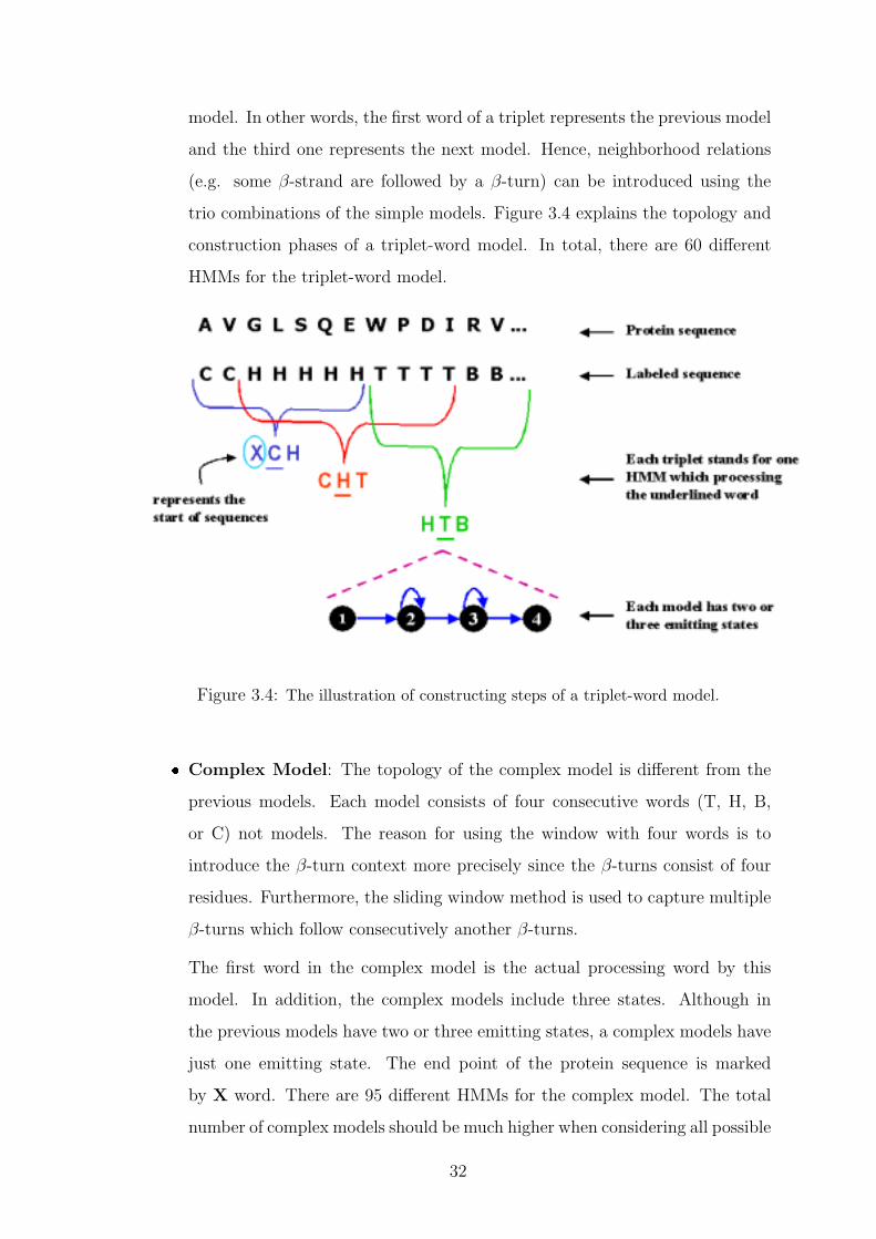
model. In other words, the first word of a triplet represents the previous model
and the third one represents the next model. Hence, neighborhood relations
(e.g. some β-strand are followed by a β-turn) can be introduced using the
trio combinations of the simple models. Figure 3.4 explains the topology and
construction phases of a triplet-word model. In total, there are 60 different
HMMs for the triplet-word model.
Figure 3.4: The illustration of constructing steps of a triplet-word model.
� Complex Model: The topology of the complex model is different from the
previous models. Each model consists of four consecutive words (T, H, B,
or C) not models. The reason for using the window with four words is to
introduce the β-turn context more precisely since the β-turns consist of four
residues. Furthermore, the sliding window method is used to capture multiple
β-turns which follow consecutively another β-turns.
The first word in the complex model is the actual processing word by this
model. In addition, the complex models include three states. Although in
the previous models have two or three emitting states, a complex models have
just one emitting state. The end point of the protein sequence is marked
by X word. There are 95 different HMMs for the complex model. The total
number of complex models should be much higher when considering all possible
32
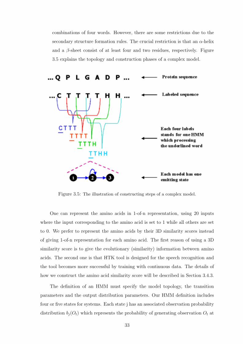
combinations of four words. However, there are some restrictions due to the
secondary structure formation rules. The crucial restriction is that an α-helix
and a β-sheet consist of at least four and two residues, respectively. Figure
3.5 explains the topology and construction phases of a complex model.
Figure 3.5: The illustration of constructing steps of a complex model.
One can represent the amino acids in 1-of-n representation, using 20 inputs
where the input corresponding to the amino acid is set to 1 while all others are set
to 0. We prefer to represent the amino acids by their 3D similarity scores instead
of giving 1-of-n representation for each amino acid. The first reason of using a 3D
similarity score is to give the evolutionary (similarity) information between amino
acids. The second one is that HTK tool is designed for the speech recognition and
the tool becomes more successful by training with continuous data. The details of
how we construct the amino acid similarity score will be described in Section 3.4.3.
The definition of an HMM must specify the model topology, the transition
parameters and the output distribution parameters. Our HMM definition includes
four or five states for systems. Each state j has an associated observation probability
distribution bj(Ot) which represents the probability of generating observation Ot at
33
time t. Each pair of states i and j has an associated transition probability aij . The
entry state and the exit state are non-emitting states.
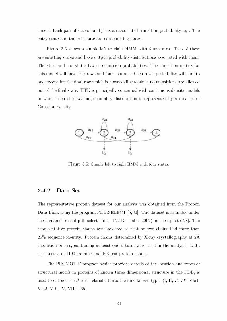
Figure 3.6 shows a simple left to right HMM with four states. Two of these
are emitting states and have output probability distributions associated with them.
The start and end states have no emission probabilities. The transition matrix for
this model will have four rows and four columns. Each row’s probability will sum to
one except for the final row which is always all zero since no transitions are allowed
out of the final state. HTK is principally concerned with continuous density models
in which each observation probability distribution is represented by a mixture of
Gaussian density.
Figure 3.6: Simple left to right HMM with four states.
3.4.2 Data Set
The representative protein dataset for our analysis was obtained from the Protein
Data Bank using the program PDB SELECT [5,30]. The dataset is available under
the filename ”recent.pdb select” (dated 22 December 2002) on the ftp site [28]. The
representative protein chains were selected so that no two chains had more than
25% sequence identity. Protein chains determined by X-ray crystallography at 2A
resolution or less, containing at least one β-turn, were used in the analysis. Data
set consists of 1190 training and 163 test protein chains.
The PROMOTIF program which provides details of the location and types of
structural motifs in proteins of known three dimensional structure in the PDB, is
used to extract the β-turns classified into the nine known types (I, II, I ′, II ′, VIa1,
VIa2, VIb, IV, VIII) [35].
34
In order to make the labeling of protein sequences, each amino acid is marked
by its secondary structure content: T, H, B, or C. We collected all the label files into
one file which is called the master label file. Another operation is to construct
the main data files whose representation is very similar to the manipulated speech
waveforms. Each amino acid is replaced with its similarity score as explained in
Section 3.4.3. Then we took a window with seven length (the total number of
amino acids) and processed each protein sequence from start to end using seven
residues window.
3.4.3 Feature Set
Amino Acid Similarity Score
In this study, an amino acid similarity matrix is used due to containing evolutionary
information between proteins and similarity between amino acids. The amino acid
similarity matrix is constructed by converting the protein similarity matrices (e.g.,
PAM, Blossom, etc.).
The protein similarity matrices are constructed by considering the evolutionary
relationships between proteins. During the evolution, some amino acids can be re-
placed by other amino acids; so, the protein similarity matrices give the probabilities
of changing from one amino acid to another. Such a similarity matrix provides the
evolutionary and similarity information about the amino acids.
We use the PAM250 similarity matrix which is 20D matrix which captures the
principal physicochemical properties of the amino acids. The PAM250 matrix is
reduced into a 3D vector since we could represent the same amino acid properties
in 3D environment [36]. The dimension reduction is done by a function mapping;
it was performed by a simple neural network that has 1 hidden layer and 3 hidden
neurons. The 20D similarity matrix is given as the input, the output is the 3D
vector for each amino acid. The 3D output vector for each amino acid is given in
Table 3.1.
35
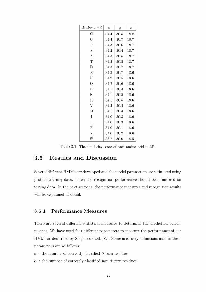
Amino Acid x y z
C 34.4 30.5 18.8G 34.4 30.7 18.7P 34.3 30.6 18.7S 34.2 30.4 18.7A 34.3 30.5 18.7T 34.2 30.5 18.7D 34.3 30.7 18.7E 34.3 30.7 18.6N 34.2 30.5 18.6Q 34.2 30.6 18.6H 34.1 30.4 18.6K 34.1 30.5 18.6R 34.1 30.5 18.6V 34.2 30.4 18.6M 34.1 30.4 18.6I 34.0 30.3 18.6L 34.0 30.3 18.6F 34.0 30.1 18.6Y 34.0 30.2 18.6W 33.7 30.0 18.5
Table 3.1: The similarity score of each amino acid in 3D.
3.5 Results and Discussion
Several different HMMs are developed and the model parameters are estimated using
protein training data. Then the recognition performance should be monitored on
testing data. In the next sections, the performance measures and recognition results
will be explained in detail.
3.5.1 Performance Measures
There are several different statistical measures to determine the prediction perfor-
mances. We have used four different parameters to measure the performance of our
HMMs as described by Shepherd et.al. [82]. Some necessary definitions used in these
parameters are as follows:
ct : the number of correctly classified β-turn residues
co : the number of correctly classified non-β-turn residues
36
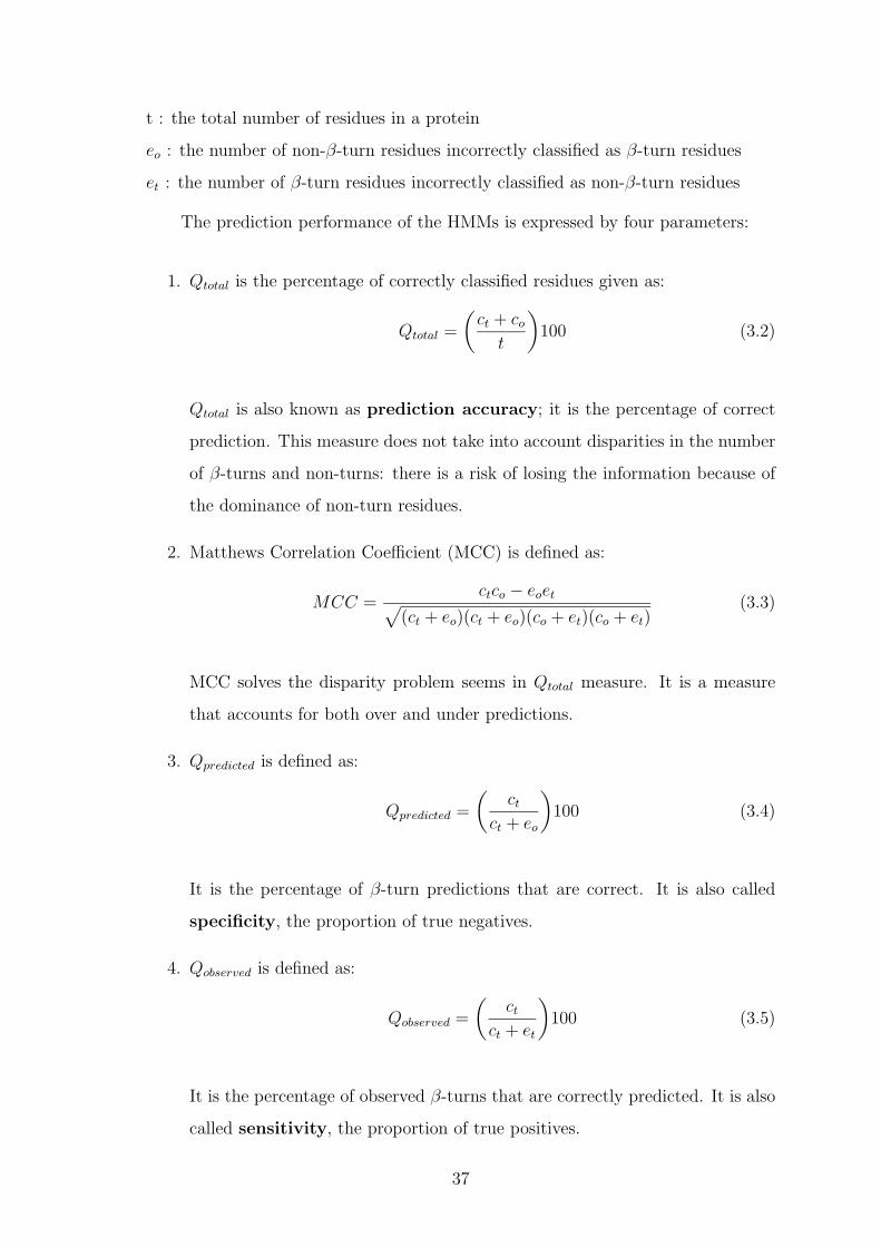
t : the total number of residues in a protein
eo : the number of non-β-turn residues incorrectly classified as β-turn residues
et : the number of β-turn residues incorrectly classified as non-β-turn residues
The prediction performance of the HMMs is expressed by four parameters:
1. Qtotal is the percentage of correctly classified residues given as:
Qtotal =
(ct + co
t
)100 (3.2)
Qtotal is also known as prediction accuracy; it is the percentage of correct
prediction. This measure does not take into account disparities in the number
of β-turns and non-turns: there is a risk of losing the information because of
the dominance of non-turn residues.
2. Matthews Correlation Coefficient (MCC) is defined as:
MCC =ctco − eoet√
(ct + eo)(ct + eo)(co + et)(co + et)(3.3)
MCC solves the disparity problem seems in Qtotal measure. It is a measure
that accounts for both over and under predictions.
3. Qpredicted is defined as:
Qpredicted =
(ct
ct + eo
)100 (3.4)
It is the percentage of β-turn predictions that are correct. It is also called
specificity, the proportion of true negatives.
4. Qobserved is defined as:
Qobserved =
(ct
ct + et
)100 (3.5)
It is the percentage of observed β-turns that are correctly predicted. It is also
called sensitivity, the proportion of true positives.
37
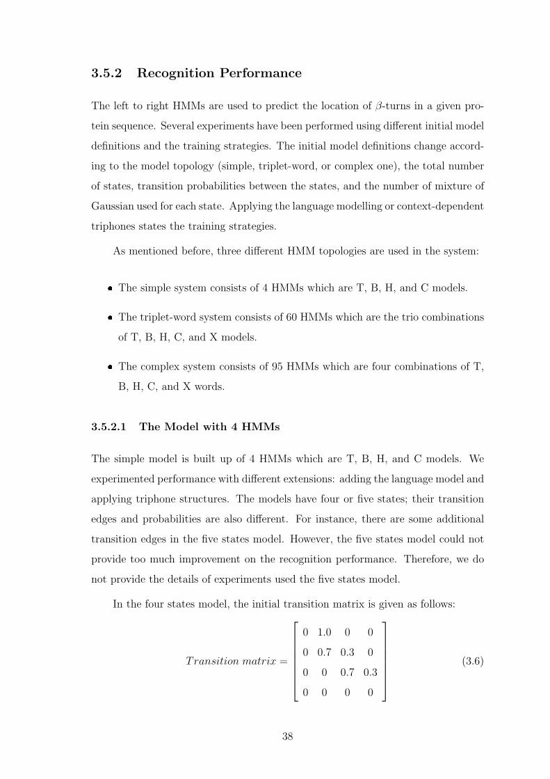
3.5.2 Recognition Performance
The left to right HMMs are used to predict the location of β-turns in a given pro-
tein sequence. Several experiments have been performed using different initial model
definitions and the training strategies. The initial model definitions change accord-
ing to the model topology (simple, triplet-word, or complex one), the total number
of states, transition probabilities between the states, and the number of mixture of
Gaussian used for each state. Applying the language modelling or context-dependent
triphones states the training strategies.
As mentioned before, three different HMM topologies are used in the system:
� The simple system consists of 4 HMMs which are T, B, H, and C models.
� The triplet-word system consists of 60 HMMs which are the trio combinations
of T, B, H, C, and X models.
� The complex system consists of 95 HMMs which are four combinations of T,
B, H, C, and X words.
3.5.2.1 The Model with 4 HMMs
The simple model is built up of 4 HMMs which are T, B, H, and C models. We
experimented performance with different extensions: adding the language model and
applying triphone structures. The models have four or five states; their transition
edges and probabilities are also different. For instance, there are some additional
transition edges in the five states model. However, the five states model could not
provide too much improvement on the recognition performance. Therefore, we do
not provide the details of experiments used the five states model.
In the four states model, the initial transition matrix is given as follows:
Transition matrix =
0 1.0 0 0
0 0.7 0.3 0
0 0 0.7 0.3
0 0 0 0
(3.6)
38
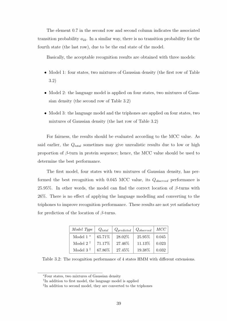
The element 0.7 in the second row and second column indicates the associated
transition probability a22. In a similar way, there is no transition probability for the
fourth state (the last row), due to be the end state of the model.
Basically, the acceptable recognition results are obtained with three models:
� Model 1: four states, two mixtures of Gaussian density (the first row of Table
3.2)
� Model 2: the language model is applied on four states, two mixtures of Gaus-
sian density (the second row of Table 3.2)
� Model 3: the language model and the triphones are applied on four states, two
mixtures of Gaussian density (the last row of Table 3.2)
For fairness, the results should be evaluated according to the MCC value. As
said earlier, the Qtotal sometimes may give unrealistic results due to low or high
proportion of β-turn in protein sequence; hence, the MCC value should be used to
determine the best performance.
The first model, four states with two mixtures of Gaussian density, has per-
formed the best recognition with 0.045 MCC value, its Qobserved performance is
25.95%. In other words, the model can find the correct location of β-turns with
26%. There is no effect of applying the language modelling and converting to the
triphones to improve recognition performance. These results are not yet satisfactory
for prediction of the location of β-turns.
Model Type Qtotal Qpredicted Qobserved MCC
Model 1 ∗ 65.71% 28.02% 25.95% 0.045
Model 2 † 71.17% 27.46% 11.13% 0.023
Model 3 ‡ 67.86% 27.45% 19.38% 0.032
Table 3.2: The recognition performance of 4 states HMM with different extensions.
∗Four states, two mixtures of Gaussian density†In addition to first model, the language model is applied‡In addition to second model, they are converted to the triphones
39
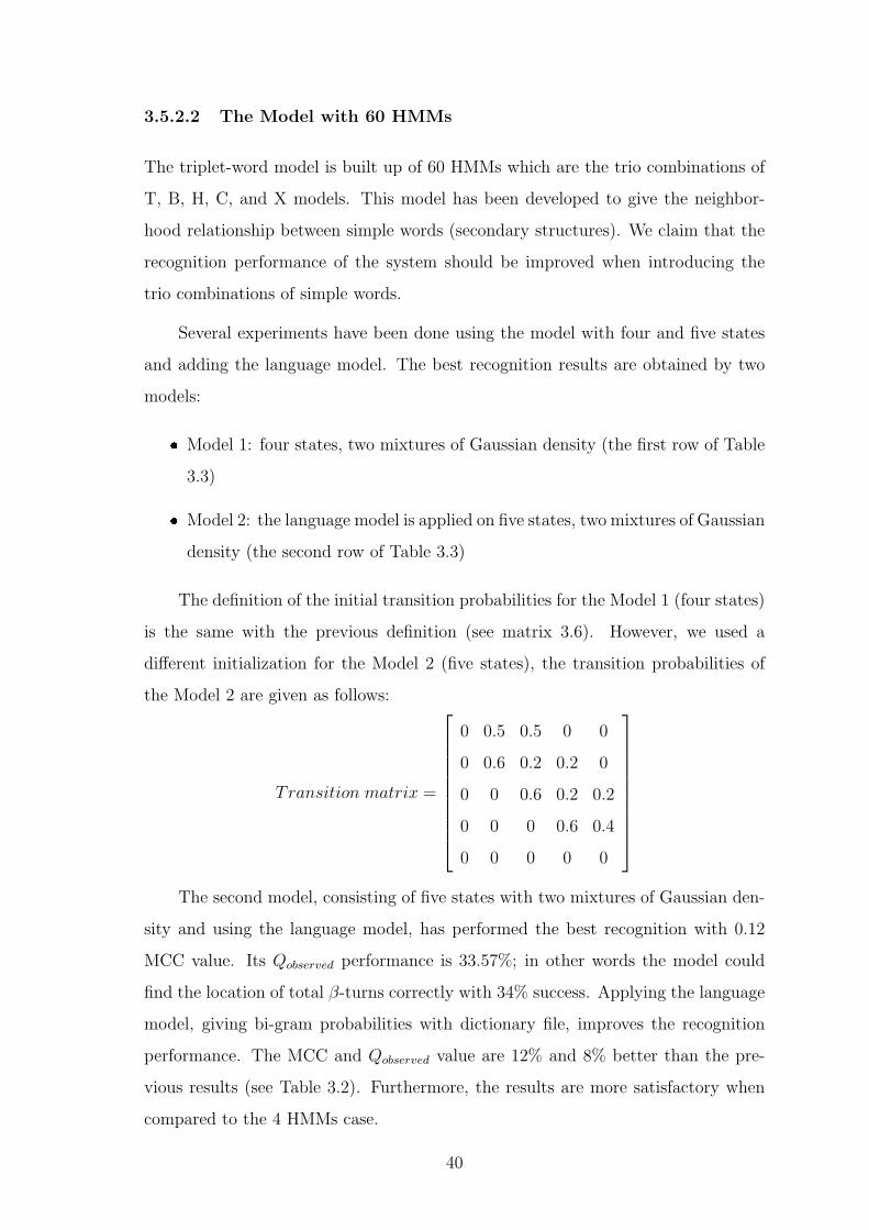
3.5.2.2 The Model with 60 HMMs
The triplet-word model is built up of 60 HMMs which are the trio combinations of
T, B, H, C, and X models. This model has been developed to give the neighbor-
hood relationship between simple words (secondary structures). We claim that the
recognition performance of the system should be improved when introducing the
trio combinations of simple words.
Several experiments have been done using the model with four and five states
and adding the language model. The best recognition results are obtained by two
models:
� Model 1: four states, two mixtures of Gaussian density (the first row of Table
3.3)
� Model 2: the language model is applied on five states, two mixtures of Gaussian
density (the second row of Table 3.3)
The definition of the initial transition probabilities for the Model 1 (four states)
is the same with the previous definition (see matrix 3.6). However, we used a
different initialization for the Model 2 (five states), the transition probabilities of
the Model 2 are given as follows:
Transition matrix =
0 0.5 0.5 0 0
0 0.6 0.2 0.2 0
0 0 0.6 0.2 0.2
0 0 0 0.6 0.4
0 0 0 0 0
The second model, consisting of five states with two mixtures of Gaussian den-
sity and using the language model, has performed the best recognition with 0.12
MCC value. Its Qobserved performance is 33.57%; in other words the model could
find the location of total β-turns correctly with 34% success. Applying the language
model, giving bi-gram probabilities with dictionary file, improves the recognition
performance. The MCC and Qobserved value are 12% and 8% better than the pre-
vious results (see Table 3.2). Furthermore, the results are more satisfactory when
compared to the 4 HMMs case.
40
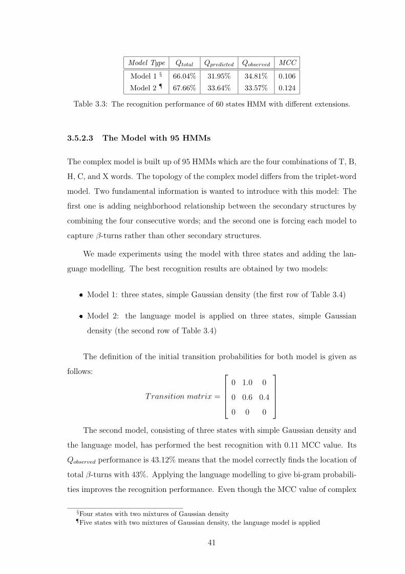
Model Type Qtotal Qpredicted Qobserved MCC
Model 1 § 66.04% 31.95% 34.81% 0.106
Model 2 ¶ 67.66% 33.64% 33.57% 0.124
Table 3.3: The recognition performance of 60 states HMM with different extensions.
3.5.2.3 The Model with 95 HMMs
The complex model is built up of 95 HMMs which are the four combinations of T, B,
H, C, and X words. The topology of the complex model differs from the triplet-word
model. Two fundamental information is wanted to introduce with this model: The
first one is adding neighborhood relationship between the secondary structures by
combining the four consecutive words; and the second one is forcing each model to
capture β-turns rather than other secondary structures.
We made experiments using the model with three states and adding the lan-
guage modelling. The best recognition results are obtained by two models:
� Model 1: three states, simple Gaussian density (the first row of Table 3.4)
� Model 2: the language model is applied on three states, simple Gaussian
density (the second row of Table 3.4)
The definition of the initial transition probabilities for both model is given as
follows:
Transition matrix =
0 1.0 0
0 0.6 0.4
0 0 0
The second model, consisting of three states with simple Gaussian density and
the language model, has performed the best recognition with 0.11 MCC value. Its
Qobserved performance is 43.12% means that the model correctly finds the location of
total β-turns with 43%. Applying the language modelling to give bi-gram probabili-
ties improves the recognition performance. Even though the MCC value of complex
§Four states with two mixtures of Gaussian density¶Five states with two mixtures of Gaussian density, the language model is applied
41
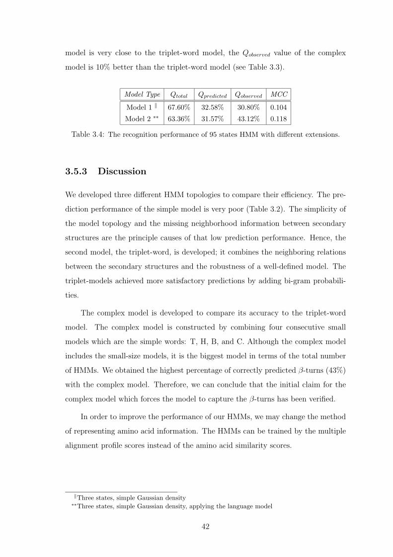
model is very close to the triplet-word model, the Qobserved value of the complex
model is 10% better than the triplet-word model (see Table 3.3).
Model Type Qtotal Qpredicted Qobserved MCC
Model 1 ‖ 67.60% 32.58% 30.80% 0.104
Model 2 ∗∗ 63.36% 31.57% 43.12% 0.118
Table 3.4: The recognition performance of 95 states HMM with different extensions.
3.5.3 Discussion
We developed three different HMM topologies to compare their efficiency. The pre-
diction performance of the simple model is very poor (Table 3.2). The simplicity of
the model topology and the missing neighborhood information between secondary
structures are the principle causes of that low prediction performance. Hence, the
second model, the triplet-word, is developed; it combines the neighboring relations
between the secondary structures and the robustness of a well-defined model. The
triplet-models achieved more satisfactory predictions by adding bi-gram probabili-
ties.
The complex model is developed to compare its accuracy to the triplet-word
model. The complex model is constructed by combining four consecutive small
models which are the simple words: T, H, B, and C. Although the complex model
includes the small-size models, it is the biggest model in terms of the total number
of HMMs. We obtained the highest percentage of correctly predicted β-turns (43%)
with the complex model. Therefore, we can conclude that the initial claim for the
complex model which forces the model to capture the β-turns has been verified.
In order to improve the performance of our HMMs, we may change the method
of representing amino acid information. The HMMs can be trained by the multiple
alignment profile scores instead of the amino acid similarity scores.
‖Three states, simple Gaussian density∗∗Three states, simple Gaussian density, applying the language model
42
3.6 Summary and Conclusion
We have worked on the prediction of β-turns in protein sequences with different
usage of HMMs. The critical role of β-turns on the folding pathway and limited
research in literature have led us to work on the problem of identifying the location
of β-turns in protein sequences. Furthermore, the absence of using HMMs in this
problem enabled the application of HMMs as the prediction method.
There are two studies working on the prediction of β-turns with its amino acid
sequence. The prediction technique, used data set, and feature of these studies
are completely different with our work; however, they are the unique works for
measuring the accuracy of our prediction system.
BTPRED is a neural network based approach [82]. They add to the input
vector the secondary structure information of a given residue obtained from the
PHDsec program [74]. The percentage of correctly predicted β-turns (Qobserved) and
MCC (without applying filtering rules) value are 31% and 0.31, respectively. When
we make a comparison of two methods, the MCC value of BTPRED is 19% better
than our complex HMM’s; however, the percentage of correctly predicted β-turns
of the complex model is 12% better than those of BTPRED’s. In BTPRED, the
introducing predicted secondary structure information of each residue in the input
vector significantly improved their performance. The absence of providing secondary
structure information makes a negative effect on the performance of our HMMs.
BetaTPred2 also uses feedforward neural networks [43]. It includes two net-
works: first feedforward network with one hidden layer is trained using multiple
sequence alignments in the PSI-BLAST form [1]. The second network is trained
by the initial prediction of the first network and PSIPRED secondary structure
information [39]. They provide a significant improvement by giving evolutionary
information with PSI-BLAST multiple alignments. The percentage of correctly pre-
dicted β-turns and MCC value are 72% and 0.43, respectively. The performance of
our HMMs could not achieve the high performance of the BetaTPred2. It is known
that using information from sequence alignments improves the secondary structure
predictions. PSI-BLAST, an improved searching tool for multiple sequence align-
ment, searches the homologous proteins against a larger database. Hence, the essen-
43
tial reason for the high performance of BetaTPred2 is its ability to give evolutionary
information effectively.
In this study, we observed the insufficiency of amino acid similarity score
against the multiple alignment profile scores. Even though we tried to introduce
the neighborhood information between secondary structures by combining simple
words (T,H,B,C), we could not introduce the evolutionary information properly.
Furthermore, the prediction errors of the α-helix, β-sheet, and coil regions have
contributed the prediction errors of β-turns; so, if we could construct a model con-
sisting of the β-turn and non-turn words, we would eliminate the error resulting
from the α-helices, β-sheets, and coils.
Actually, HMM has performed the prediction of β-turns merely using the amino
acid similarity scores quite well. If we had used the PSI-BLAST multiple alignment
scores instead of the amino acid similarity scores, the prediction performance of the
HMM would have been much better. As an initial work, we obtained promising
results for the β-turn prediction problem using HMMs.
3.7 Usage of Hidden Markov Model Toolkit
The Hidden Markov Model Toolkit (HTK) is applied to predict the location of β-
turns in a given protein sequence [32]. The HTK is a portable toolkit for building
and manipulating HMMs. HMMs can be used to model any time series and the
core of HTK is similarly general-purpose. HTK is primarily used for speech recog-
nition research although it has been used for numerous other applications including
research into speech synthesis, character recognition and DNA sequencing.
There are two major processing stages involved. Firstly, the HTK training tools
are used to estimate the parameters of a set of HMMs using training utterances and
their associated transcriptions. Secondly, unknown utterances are transcribed using
the HTK recognition tools.
HTK is built into the library modules. These modules ensure that every tool
interfaces to the outside world in exactly the same way. They also provide a central
resource of commonly used functions. Figure 3.7 illustrates the software structure
44
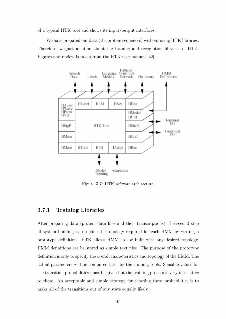
of a typical HTK tool and shows its input/output interfaces.
We have prepared our data (the protein sequences) without using HTK libraries.
Therefore, we just mention about the training and recognition libraries of HTK.
Figures and review is taken from the HTK user manual [32].
Figure 3.7: HTK software architecture.
3.7.1 Training Libraries
After preparing data (protein data files and their transcriptions), the second step
of system building is to define the topology required for each HMM by writing a
prototype definition. HTK allows HMMs to be built with any desired topology.
HMM definitions are be stored as simple text files. The purpose of the prototype
definition is only to specify the overall characteristics and topology of the HMM. The
actual parameters will be computed later by the training tools. Sensible values for
the transition probabilities must be given but the training process is very insensitive
to these. An acceptable and simple strategy for choosing these probabilities is to
make all of the transitions out of any state equally likely.
45
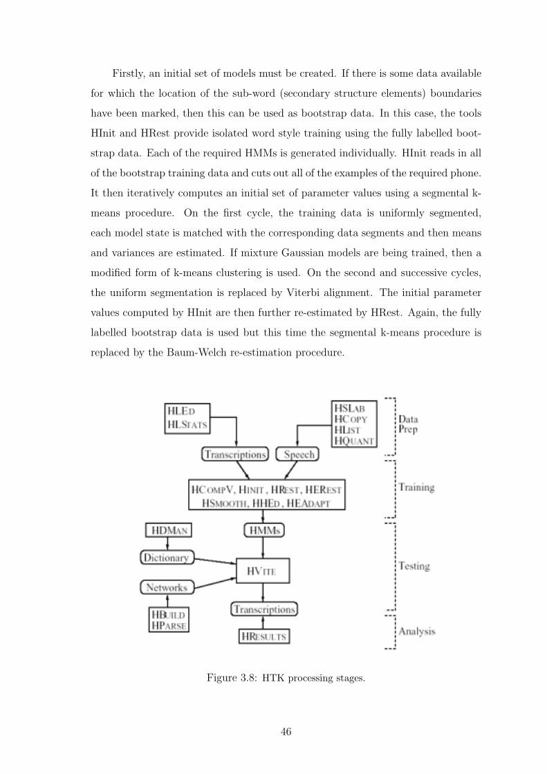
Firstly, an initial set of models must be created. If there is some data available
for which the location of the sub-word (secondary structure elements) boundaries
have been marked, then this can be used as bootstrap data. In this case, the tools
HInit and HRest provide isolated word style training using the fully labelled boot-
strap data. Each of the required HMMs is generated individually. HInit reads in all
of the bootstrap training data and cuts out all of the examples of the required phone.
It then iteratively computes an initial set of parameter values using a segmental k-
means procedure. On the first cycle, the training data is uniformly segmented,
each model state is matched with the corresponding data segments and then means
and variances are estimated. If mixture Gaussian models are being trained, then a
modified form of k-means clustering is used. On the second and successive cycles,
the uniform segmentation is replaced by Viterbi alignment. The initial parameter
values computed by HInit are then further re-estimated by HRest. Again, the fully
labelled bootstrap data is used but this time the segmental k-means procedure is
replaced by the Baum-Welch re-estimation procedure.
Figure 3.8: HTK processing stages.
46
Once an initial set of models has been created, the tool HERest is used to
perform embedded training using the entire training set. HERest performs a single
Baum-Welch re-estimation of the whole set of HMM phone models simultaneously.
For each training utterance, the corresponding models are concatenated and then the
forward-backward algorithm is used to accumulate the statistics of state occupation,
means, variances, etc., for each HMM in the sequence. When all of the training data
has been processed, the accumulated statistics are used to compute re-estimates
of the HMM parameters. The philosophy of system construction in HTK is that
HMMs should be refined incrementally. Thus, a typical progression is to start with a
simple set of single Gaussian context-independent models and then iteratively refine
them by expanding them to include context-dependency and use multiple mixture
component Gaussian distributions. The tool HHEd is an HMM definition editor
which will clone models into context-dependent sets, apply a variety of parameter
tyings and increment the number of mixture components in specified distributions.
The usual process is to modify a set of HMMs in stages using HHEd and then re-
estimate the parameters of the modified set using HERest after each stage. The
more complex the model set, the more data is needed to make robust estimates of
its parameters, and since data is usually limited, a balance must be struck between
complexity and the available data.
3.7.2 Recognition Libraries
The HTK tool can perform the Viterbi-based recognition. It takes the word network
and then attaches the appropriate HMM definition to each word instance. Then the
recognition is performed on the list of test files. HTK provides a single recognition
tool called HVite which uses the token passing algorithm to perform Viterbi-based
recognition. HVite takes as input a network describing the allowable word sequences,
a dictionary defining how each word is pronounced and a set of HMMs. According
to speech terminology, a word is pronounced as the sequence of phones p1 p2 p3
etc. Hence, the dictionary file keeps all possible words and their pronunciations.
For β-turn prediction problem, no need to give pronunciation of words (T, H, B,
C) in a special way; because, we don’t want to find the pronunciation of a given
47
word or vice versa. Actually, the aim is to identify the words (T, H, B, or C) of
a given protein sequence; so, we leave pronunciations the same with words. HVite
operates by converting the word network to a phone network and then attaching
the appropriate HMM definition to each phone instance. Recognition can then be
performed on the list of stored test files. HVite can support cross-word triphones and
it can run with multiple tokens to generate lattices containing multiple hypotheses.
The word networks needed to drive HVite are usually either simple word loops in
which any word can follow any other word or they are directed graphs representing
a finite-state task grammar. In the former case, bi-gram probabilities are normally
attached to the word transitions.
HBuild allows sub-networks to be created and used within higher level networks.
HBuild can be used to generate word loops and it can also read in a backed-off
bi-gram language model and modify the word loop transitions to incorporate the
bi-gram probabilities. Note that the label statistics tool HLStats can be used to
generate a backed-off bi-gram language model. As an alternative to specifying a
word network directly, a higher level grammar notation can be used. This notation
is based on the Extended Backus Naur Form (EBNF) used in compiler specification
and it is compatible with the grammar specification language. The tool HParse is
supplied to convert this notation into the equivalent word network.
3.7.3 Language Modelling
A described in the previous section, HTK tool needs a network describing the allow-
able word sequences, during the recognition phase. The word networks needed to
drive either simple word loops in which any word can follow any other word or they
are directed graphs representing a finite-state task grammar. The bi-gram proba-
bilities are attached to the word transitions and they provide a prior information
about the consecutive word relations. In order to calculate the bi-gram probabilities
we should apply the language modelling to the training data.
The HTK language modelling tools are designed for constructing and testing
statistical n-gram language models. An n-gram is a sequence of n symbols and an
n-gram language model (LM) is used to predict each symbol in the sequence given
48
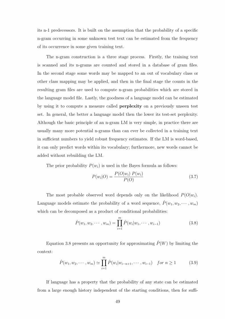
its n-1 predecessors. It is built on the assumption that the probability of a specific
n-gram occurring in some unknown test text can be estimated from the frequency
of its occurrence in some given training text.
The n-gram construction is a three stage process. Firstly, the training text
is scanned and its n-grams are counted and stored in a database of gram files.
In the second stage some words may be mapped to an out of vocabulary class or
other class mapping may be applied, and then in the final stage the counts in the
resulting gram files are used to compute n-gram probabilities which are stored in
the language model file. Lastly, the goodness of a language model can be estimated
by using it to compute a measure called perplexity on a previously unseen test
set. In general, the better a language model then the lower its test-set perplexity.
Although the basic principle of an n-gram LM is very simple, in practice there are
usually many more potential n-grams than can ever be collected in a training text
in sufficient numbers to yield robust frequency estimates. If the LM is word-based,
it can only predict words within its vocabulary; furthermore, new words cannot be
added without rebuilding the LM.
The prior probability P (wi) is used in the Bayes formula as follows:
P (wi|O) =P (O|wi) P (wi)
P (O)(3.7)
The most probable observed word depends only on the likelihood P (O|wi).
Language models estimate the probability of a word sequence, P (w1, w2, · · · , wm)
which can be decomposed as a product of conditional probabilities:
P (w1, w2, · · · , wm) =m∏
i=1
P (wi|w1, · · · , wi−1) (3.8)
Equation 3.8 presents an opportunity for approximating P (W ) by limiting the
context:
P (w1, w2, · · · , wm) �m∏
i=1
P (wi|wi−n+1, · · · , wi−1) for n ≥ 1 (3.9)
If language has a property that the probability of any state can be estimated
from a large enough history independent of the starting conditions, then for suffi-
49
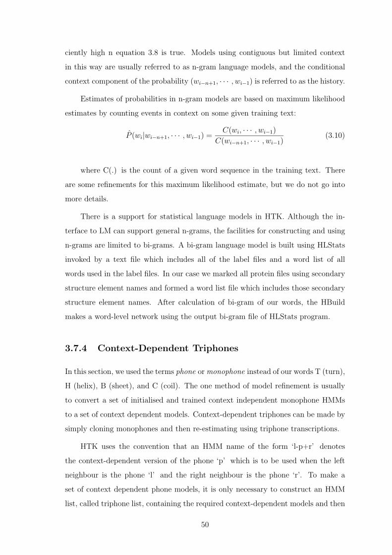
ciently high n equation 3.8 is true. Models using contiguous but limited context
in this way are usually referred to as n-gram language models, and the conditional
context component of the probability (wi−n+1, · · · , wi−1) is referred to as the history.
Estimates of probabilities in n-gram models are based on maximum likelihood
estimates by counting events in context on some given training text:
P (wi|wi−n+1, · · · , wi−1) =C(wi, · · · , wi−1)
C(wi−n+1, · · · , wi−1)(3.10)
where C(.) is the count of a given word sequence in the training text. There
are some refinements for this maximum likelihood estimate, but we do not go into
more details.
There is a support for statistical language models in HTK. Although the in-
terface to LM can support general n-grams, the facilities for constructing and using
n-grams are limited to bi-grams. A bi-gram language model is built using HLStats
invoked by a text file which includes all of the label files and a word list of all
words used in the label files. In our case we marked all protein files using secondary
structure element names and formed a word list file which includes those secondary
structure element names. After calculation of bi-gram of our words, the HBuild
makes a word-level network using the output bi-gram file of HLStats program.
3.7.4 Context-Dependent Triphones
In this section, we used the terms phone or monophone instead of our words T (turn),
H (helix), B (sheet), and C (coil). The one method of model refinement is usually
to convert a set of initialised and trained context independent monophone HMMs
to a set of context dependent models. Context-dependent triphones can be made by
simply cloning monophones and then re-estimating using triphone transcriptions.
HTK uses the convention that an HMM name of the form ‘l-p+r’ denotes
the context-dependent version of the phone ‘p’ which is to be used when the left
neighbour is the phone ‘l’ and the right neighbour is the phone ‘r’. To make a
set of context dependent phone models, it is only necessary to construct an HMM
list, called triphone list, containing the required context-dependent models and then
50
execute HHEd program that makes a copy of the monophone ‘p’ for each model
‘l-p+r’ in triphone list. The set of context-dependent models output by the above
must be re-estimated using HERest. To do this, the training data transcriptions
must be converted to use context-dependent labels and the original monophone
hmm list must be replaced by triphone list. In fact, it is best to do this conversion
before cloning the monophones because the HLEd program can be used to generate
the required list of context dependent HMMs automatically.
Before building a set of context-dependent models, it is necessary to decide
whether or not cross-word triphones are to be used. Tying could affect performance if
performed indiscriminately. Hence, it is important to only tie parameters which have
little effect on discrimination. If the transition parameters do not vary significantly
with context but nevertheless need to be estimated accurately. Some triphones will
occur only once or twice and so very poor estimates would be obtained if tying
was not done. These problems of data insufficiency will also affect the output
distributions.
51
Chapter 4
The Classification of The β-Turns by
Artificial Neural Networks
4.1 Introduction
The β-turns are not unified structures; they include different types. Hence, identi-
fying the location of the β-turns in protein sequence is insufficient; type of β-turns
would also be useful. Even though there are few studies on identification of the
β-turn regions, the work on identifying the type of the β-turns is even more limited.
We have attempted to find the location of β-turns using HMMs in Chapter 3. As
a second step, we wanted to extend this study on type classification of β-turns by
using Artificial Neural Networks.
The critical roles of β-turns on the protein fold should not be underestimated
since the β-turns comprise on the average 25% of the residues in the globular proteins
[40] and change the direction of the amino acid chain. In addition, β-turns reside
on the surface of the protein and interact with other proteins or molecules; hence
the identification of the location and type of the β-turns may give clues about the
interaction of a protein with other proteins.
52
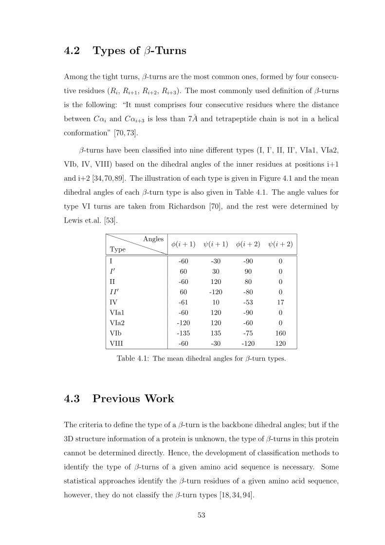
4.2 Types of β-Turns
Among the tight turns, β-turns are the most common ones, formed by four consecu-
tive residues (Ri, Ri+1, Ri+2, Ri+3). The most commonly used definition of β-turns
is the following: “It must comprises four consecutive residues where the distance
between Cαi and Cαi+3 is less than 7A and tetrapeptide chain is not in a helical
conformation” [70,73].
β-turns have been classified into nine different types (I, I’, II, II’, VIa1, VIa2,
VIb, IV, VIII) based on the dihedral angles of the inner residues at positions i+1
and i+2 [34,70,89]. The illustration of each type is given in Figure 4.1 and the mean
dihedral angles of each β-turn type is also given in Table 4.1. The angle values for
type VI turns are taken from Richardson [70], and the rest were determined by
Lewis et.al. [53].
����������TypeAngles
φ(i + 1) ψ(i + 1) φ(i + 2) ψ(i + 2)
I -60 -30 -90 0I ′ 60 30 90 0II -60 120 80 0II ′ 60 -120 -80 0IV -61 10 -53 17VIa1 -60 120 -90 0VIa2 -120 120 -60 0VIb -135 135 -75 160VIII -60 -30 -120 120
Table 4.1: The mean dihedral angles for β-turn types.
4.3 Previous Work
The criteria to define the type of a β-turn is the backbone dihedral angles; but if the
3D structure information of a protein is unknown, the type of β-turns in this protein
cannot be determined directly. Hence, the development of classification methods to
identify the type of β-turns of a given amino acid sequence is necessary. Some
statistical approaches identify the β-turn residues of a given amino acid sequence,
however, they do not classify the β-turn types [18,34,94].
53
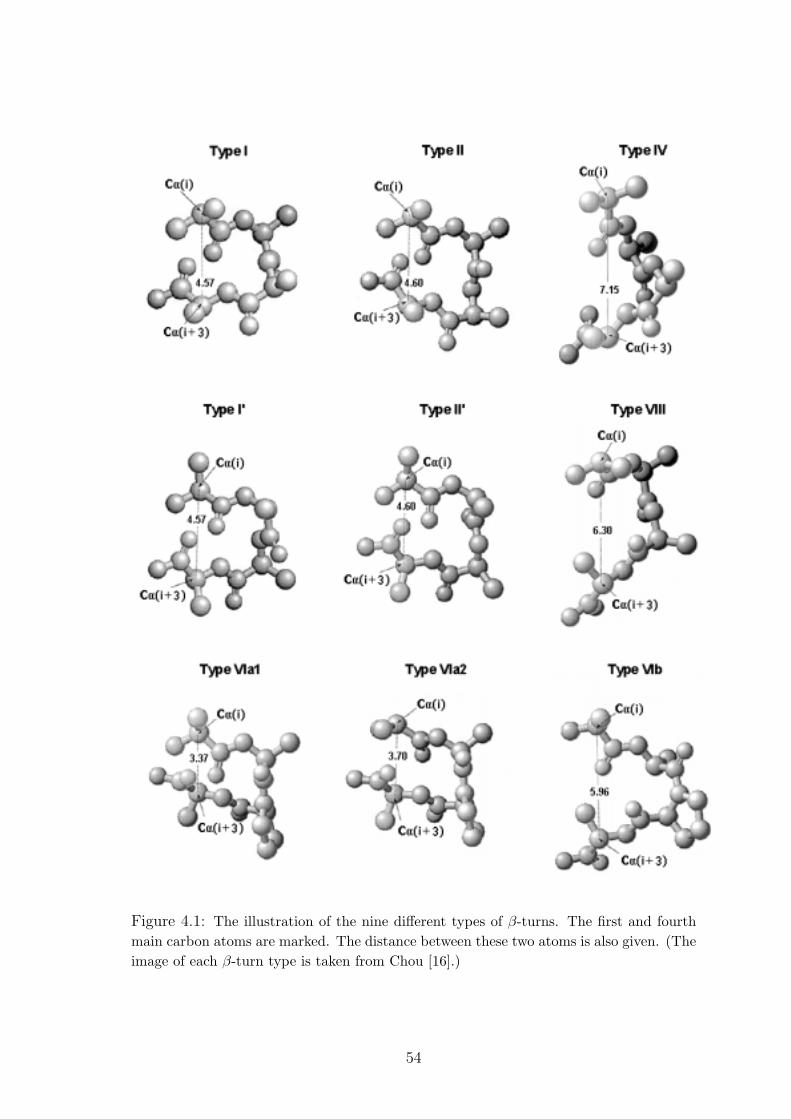
Figure 4.1: The illustration of the nine different types of β-turns. The first and fourthmain carbon atoms are marked. The distance between these two atoms is also given. (Theimage of each β-turn type is taken from Chou [16].)
54
Two studies working on the classification of the β-turn types are noteworthy.
The first one is BTPRED which is a neural network based method using a feedfor-
ward neural network with one hidden layer [82]. The input vector is formed using
binary encoding. In other words, each amino acid is represented by a single one
and nineteen zeros, giving an 80 dimensional input vector. In addition, they use the
secondary structure information (α-helix, β-sheet or coil) obtained from the PHDsec
program. So, the total dimension of their input vector increases to 83. The β-turn
type classification performance is different for each class because of the unbalanced
data in each class. Their average test performance for the four β-turn types is near
36%.
The second work classifying the type of β-turns uses SVM as the classification
tool [11]. As in the previous work, the input vector is formed using binary encoding;
each β-turn is represented by an 80 dimensional vector. The β-turn type classifi-
cation performance (training performance) is 98% on the average. However, this
performance is obtained from the training data, no test performance was given.
4.4 Our Method
A Multilayer Perceptron (MLP) is used to classify the type of β-turns. MLPs
are one of the commonly used types of Artificial Neural Networks (ANN) for the
supervised classification tasks. The detail information about ANNs and the training
algorithm is explained in Appendix C.
In this study, the MLP consists of an input layer, one hidden layer, and an
output layer. The input vector, representing a β-turn sequence, is feed to the input
layer of the MLP and the network is trained to output the type (class) of this β-
turn. The input vector has 12, 17, or 18 dimensions. The content of each one will
be explained in Section 4.4.2. The number of neurons for the hidden layer varies
between 10 and 20. The number of the output nodes is the total number of β-turn
classes using the one-of-c encoding for the classification, as shown in Figure 4.2.
The target value of output nodes is assigned to 0.9 for the desired class, and 0.1
for other classes. A threshold is set to decide when the winning node’s activation
55
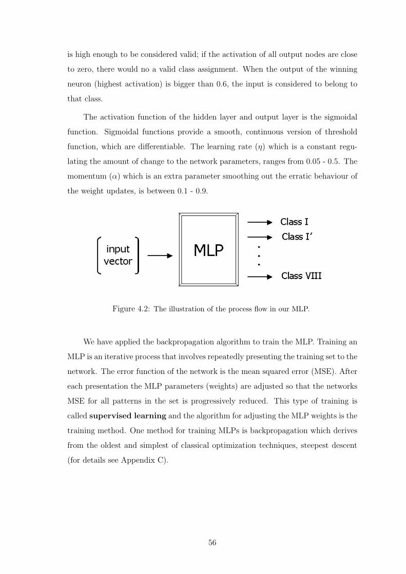
is high enough to be considered valid; if the activation of all output nodes are close
to zero, there would no a valid class assignment. When the output of the winning
neuron (highest activation) is bigger than 0.6, the input is considered to belong to
that class.
The activation function of the hidden layer and output layer is the sigmoidal
function. Sigmoidal functions provide a smooth, continuous version of threshold
function, which are differentiable. The learning rate (η) which is a constant regu-
lating the amount of change to the network parameters, ranges from 0.05 - 0.5. The
momentum (α) which is an extra parameter smoothing out the erratic behaviour of
the weight updates, is between 0.1 - 0.9.
Figure 4.2: The illustration of the process flow in our MLP.
We have applied the backpropagation algorithm to train the MLP. Training an
MLP is an iterative process that involves repeatedly presenting the training set to the
network. The error function of the network is the mean squared error (MSE). After
each presentation the MLP parameters (weights) are adjusted so that the networks
MSE for all patterns in the set is progressively reduced. This type of training is
called supervised learning and the algorithm for adjusting the MLP weights is the
training method. One method for training MLPs is backpropagation which derives
from the oldest and simplest of classical optimization techniques, steepest descent
(for details see Appendix C).
56
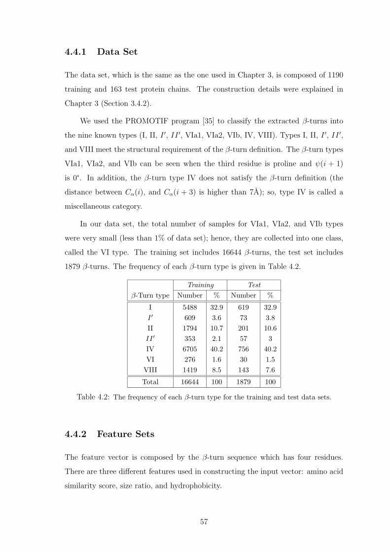
4.4.1 Data Set
The data set, which is the same as the one used in Chapter 3, is composed of 1190
training and 163 test protein chains. The construction details were explained in
Chapter 3 (Section 3.4.2).
We used the PROMOTIF program [35] to classify the extracted β-turns into
the nine known types (I, II, I ′, II ′, VIa1, VIa2, VIb, IV, VIII). Types I, II, I ′, II ′,
and VIII meet the structural requirement of the β-turn definition. The β-turn types
VIa1, VIa2, and VIb can be seen when the third residue is proline and ψ(i + 1)
is 0�. In addition, the β-turn type IV does not satisfy the β-turn definition (the
distance between Cα(i), and Cα(i + 3) is higher than 7A); so, type IV is called a
miscellaneous category.
In our data set, the total number of samples for VIa1, VIa2, and VIb types
were very small (less than 1% of data set); hence, they are collected into one class,
called the VI type. The training set includes 16644 β-turns, the test set includes
1879 β-turns. The frequency of each β-turn type is given in Table 4.2.
Training Testβ-Turn type Number % Number %
I 5488 32.9 619 32.9I ′ 609 3.6 73 3.8II 1794 10.7 201 10.6II ′ 353 2.1 57 3IV 6705 40.2 756 40.2VI 276 1.6 30 1.5
VIII 1419 8.5 143 7.6
Total 16644 100 1879 100
Table 4.2: The frequency of each β-turn type for the training and test data sets.
4.4.2 Feature Sets
The feature vector is composed by the β-turn sequence which has four residues.
There are three different features used in constructing the input vector: amino acid
similarity score, size ratio, and hydrophobicity.
57
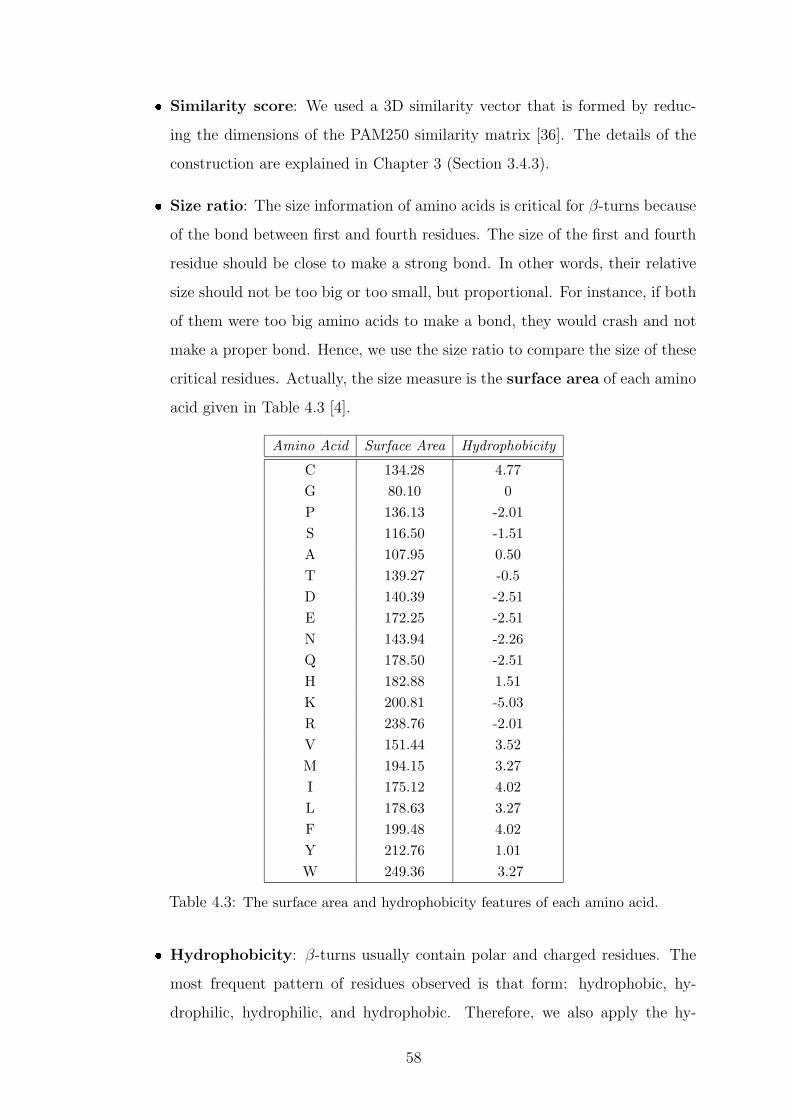
� Similarity score: We used a 3D similarity vector that is formed by reduc-
ing the dimensions of the PAM250 similarity matrix [36]. The details of the
construction are explained in Chapter 3 (Section 3.4.3).
� Size ratio: The size information of amino acids is critical for β-turns because
of the bond between first and fourth residues. The size of the first and fourth
residue should be close to make a strong bond. In other words, their relative
size should not be too big or too small, but proportional. For instance, if both
of them were too big amino acids to make a bond, they would crash and not
make a proper bond. Hence, we use the size ratio to compare the size of these
critical residues. Actually, the size measure is the surface area of each amino
acid given in Table 4.3 [4].
Amino Acid Surface Area Hydrophobicity
C 134.28 4.77G 80.10 0P 136.13 -2.01S 116.50 -1.51A 107.95 0.50T 139.27 -0.5D 140.39 -2.51E 172.25 -2.51N 143.94 -2.26Q 178.50 -2.51H 182.88 1.51K 200.81 -5.03R 238.76 -2.01V 151.44 3.52M 194.15 3.27I 175.12 4.02L 178.63 3.27F 199.48 4.02Y 212.76 1.01W 249.36 3.27
Table 4.3: The surface area and hydrophobicity features of each amino acid.
� Hydrophobicity: β-turns usually contain polar and charged residues. The
most frequent pattern of residues observed is that form: hydrophobic, hy-
drophilic, hydrophilic, and hydrophobic. Therefore, we also apply the hy-
58
drophobicity feature to consider that information. The hydrophobicity value
of each amino acid is also given in Table 4.3.
Three different input vectors with different dimensions are constructed. Before
using input vectors, they are normalized to have zero mean and unit variance. Each
input vector includes the following features:
� 12 dimension: includes only the amino acid similarity scores. A β-turn consists
of four residues and the 3D similarity score is used for each one.
� 17 dimension: Addition to amino acid similarity scores (12), the size ratio of
the first and fourth residues (1), and the hydrophobicity value of each residue
(4) are also used.
� 18 dimension: The amino acid similarity scores (12), the size ratio of the first
and fourth residues (1), the size ratio of the second and third residues (1), and
the hydrophobicity value of each residue (4) are used.
4.5 Results and Discussion
We have performed the training and test for three different cases by using the
following input vectors:
1. 12 dimensional
2. 17 dimensional
3. 18 dimensional
Although the classification performances of the 17D and 18D vectors are very
similar, the 17D input vector performed the best one. The sigmoid and tangent
activation functions in the MLP layers provide identical performance. The detailed
results will be given in the following sections.
59
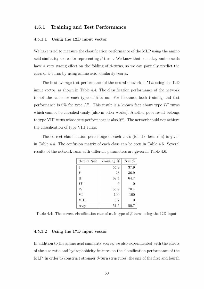
4.5.1 Training and Test Performance
4.5.1.1 Using the 12D input vector
We have tried to measure the classification performance of the MLP using the amino
acid similarity scores for representing β-turns. We know that some key amino acids
have a very strong effect on the folding of β-turns, so we can partially predict the
class of β-turns by using amino acid similarity scores.
The best average test performance of the neural network is 51% using the 12D
input vector, as shown in Table 4.4. The classification performance of the network
is not the same for each type of β-turns. For instance, both training and test
performance is 0% for type II ′. This result is a known fact about type II ′ turns
which cannot be classified easily (also in other works). Another poor result belongs
to type VIII turns whose test performance is also 0%. The network could not achieve
the classification of type VIII turns.
The correct classification percentage of each class (for the best run) is given
in Table 4.4. The confusion matrix of each class can be seen in Table 4.5. Several
results of the network runs with different parameters are given in Table 4.6.
β-turn type Training % Test %
I 55.9 37.9I ′ 28 36.9II 62.4 64.7II ′ 0 0IV 58.9 70.4VI 100 100VIII 0.7 0Avg: 51.5 50.7
Table 4.4: The correct classification rate of each type of β-turns using the 12D input.
4.5.1.2 Using the 17D input vector
In addition to the amino acid similarity scores, we also experimented with the effects
of the size ratio and hydrophobicity features on the classification performance of the
MLP. In order to construct stronger β-turn structures, the size of the first and fourth
60
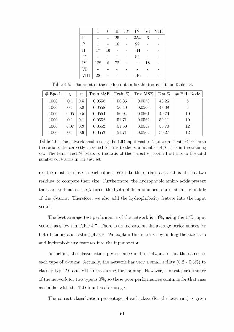
I I ′ II II ′ IV VI VIIII - - 25 - 354 6 -I ′ 1 - 16 - 29 - -II 17 10 - - 44 - -II ′ - 1 1 - 55 - -IV 128 6 72 - - 18 -VI - - - - - - -VIII 28 - - - 116 - -
Table 4.5: The count of the confused data for the test results in Table 4.4.
# Epoch η α Train MSE Train % Test MSE Test % # Hid. Node
1000 0.1 0.5 0.0558 50.35 0.0570 48.25 81000 0.1 0.9 0.0558 50.46 0.0566 48.09 81000 0.05 0.5 0.0554 50.94 0.0561 49.79 101000 0.1 0.1 0.0552 51.71 0.0562 50.11 101000 0.07 0.9 0.0552 51.50 0.0559 50.70 121000 0.1 0.9 0.0552 51.71 0.0562 50.27 12
Table 4.6: The network results using the 12D input vector. The term “Train %”refers tothe ratio of the correctly classified β-turns to the total number of β-turns in the trainingset. The term “Test %”refers to the ratio of the correctly classified β-turns to the totalnumber of β-turns in the test set.
residue must be close to each other. We take the surface area ratios of that two
residues to compare their size. Furthermore, the hydrophobic amino acids present
the start and end of the β-turns; the hydrophilic amino acids present in the middle
of the β-turns. Therefore, we also add the hydrophobicity feature into the input
vector.
The best average test performance of the network is 53%, using the 17D input
vector, as shown in Table 4.7. There is an increase on the average performances for
both training and testing phases. We explain this increase by adding the size ratio
and hydrophobicity features into the input vector.
As before, the classification performance of the network is not the same for
each type of β-turns. Actually, the network has very a small ability (0.2 - 0.3%) to
classify type II ′ and VIII turns during the training. However, the test performance
of the network for two type is 0%, so these poor performances continue for that case
as similar with the 12D input vector usage.
The correct classification percentage of each class (for the best run) is given
61
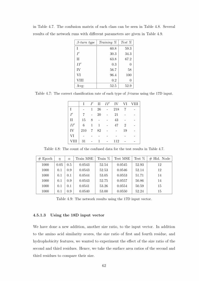
in Table 4.7. The confusion matrix of each class can be seen in Table 4.8. Several
results of the network runs with different parameters are given in Table 4.9.
β-turn type Training % Test %
I 60.8 59.3I ′ 30.3 34.3II 63.8 67.2II ′ 0.3 0IV 56.7 58VI 96.4 100VIII 0.2 0Avg: 52.5 52.9
Table 4.7: The correct classification rate of each type of β-turns using the 17D input.
I I ′ II II ′ IV VI VIIII - 1 26 - 218 7 -I ′ 7 - 20 - 21 - -II 15 8 - - 43 - -II ′ 6 1 1 - 47 2 -IV 210 7 82 - - 19 -VI - - - - - - -VIII 31 - 1 - 112 - -
Table 4.8: The count of the confused data for the test results in Table 4.7.
# Epoch η α Train MSE Train % Test MSE Test % # Hid. Node
1000 0.05 0.5 0.0543 52.54 0.0545 52.93 121000 0.1 0.9 0.0543 52.53 0.0546 52.14 121000 0.1 0.1 0.0544 53.05 0.0553 51.71 141000 0.1 0.9 0.0543 52.75 0.0557 50.86 141000 0.1 0.1 0.0541 53.26 0.0554 50.59 151000 0.1 0.9 0.0540 53.00 0.0550 52.24 15
Table 4.9: The network results using the 17D input vector.
4.5.1.3 Using the 18D input vector
We have done a new addition, another size ratio, to the input vector. In addition
to the amino acid similarity scores, the size ratio of first and fourth residue, and
hydrophobicity features, we wanted to experiment the effect of the size ratio of the
second and third residues. Hence, we take the surface area ratios of the second and
third residues to compare their size.
62
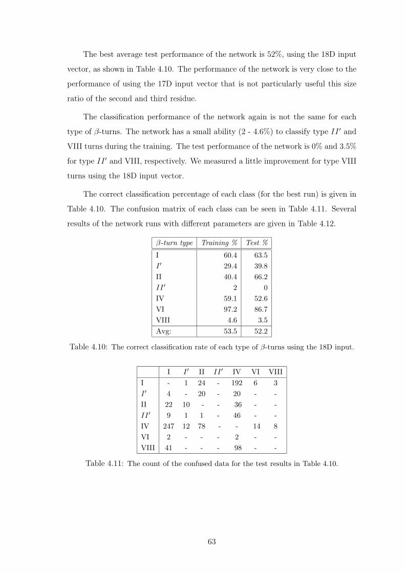
The best average test performance of the network is 52%, using the 18D input
vector, as shown in Table 4.10. The performance of the network is very close to the
performance of using the 17D input vector that is not particularly useful this size
ratio of the second and third residue.
The classification performance of the network again is not the same for each
type of β-turns. The network has a small ability (2 - 4.6%) to classify type II ′ and
VIII turns during the training. The test performance of the network is 0% and 3.5%
for type II ′ and VIII, respectively. We measured a little improvement for type VIII
turns using the 18D input vector.
The correct classification percentage of each class (for the best run) is given in
Table 4.10. The confusion matrix of each class can be seen in Table 4.11. Several
results of the network runs with different parameters are given in Table 4.12.
β-turn type Training % Test %
I 60.4 63.5I ′ 29.4 39.8II 40.4 66.2II ′ 2 0IV 59.1 52.6VI 97.2 86.7VIII 4.6 3.5Avg: 53.5 52.2
Table 4.10: The correct classification rate of each type of β-turns using the 18D input.
I I ′ II II ′ IV VI VIIII - 1 24 - 192 6 3I ′ 4 - 20 - 20 - -II 22 10 - - 36 - -II ′ 9 1 1 - 46 - -IV 247 12 78 - - 14 8VI 2 - - - 2 - -VIII 41 - - - 98 - -
Table 4.11: The count of the confused data for the test results in Table 4.10.
63
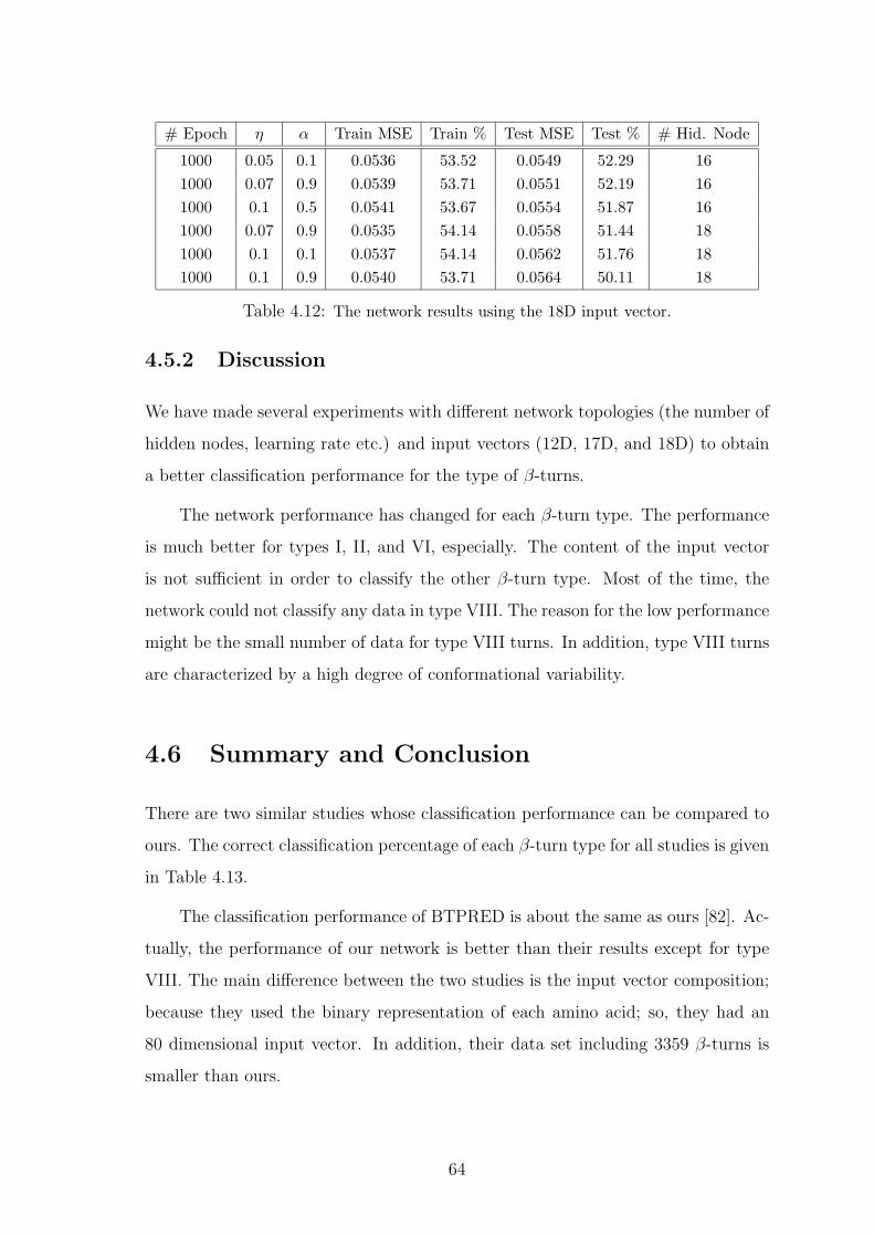
# Epoch η α Train MSE Train % Test MSE Test % # Hid. Node
1000 0.05 0.1 0.0536 53.52 0.0549 52.29 161000 0.07 0.9 0.0539 53.71 0.0551 52.19 161000 0.1 0.5 0.0541 53.67 0.0554 51.87 161000 0.07 0.9 0.0535 54.14 0.0558 51.44 181000 0.1 0.1 0.0537 54.14 0.0562 51.76 181000 0.1 0.9 0.0540 53.71 0.0564 50.11 18
Table 4.12: The network results using the 18D input vector.
4.5.2 Discussion
We have made several experiments with different network topologies (the number of
hidden nodes, learning rate etc.) and input vectors (12D, 17D, and 18D) to obtain
a better classification performance for the type of β-turns.
The network performance has changed for each β-turn type. The performance
is much better for types I, II, and VI, especially. The content of the input vector
is not sufficient in order to classify the other β-turn type. Most of the time, the
network could not classify any data in type VIII. The reason for the low performance
might be the small number of data for type VIII turns. In addition, type VIII turns
are characterized by a high degree of conformational variability.
4.6 Summary and Conclusion
There are two similar studies whose classification performance can be compared to
ours. The correct classification percentage of each β-turn type for all studies is given
in Table 4.13.
The classification performance of BTPRED is about the same as ours [82]. Ac-
tually, the performance of our network is better than their results except for type
VIII. The main difference between the two studies is the input vector composition;
because they used the binary representation of each amino acid; so, they had an
80 dimensional input vector. In addition, their data set including 3359 β-turns is
smaller than ours.
64
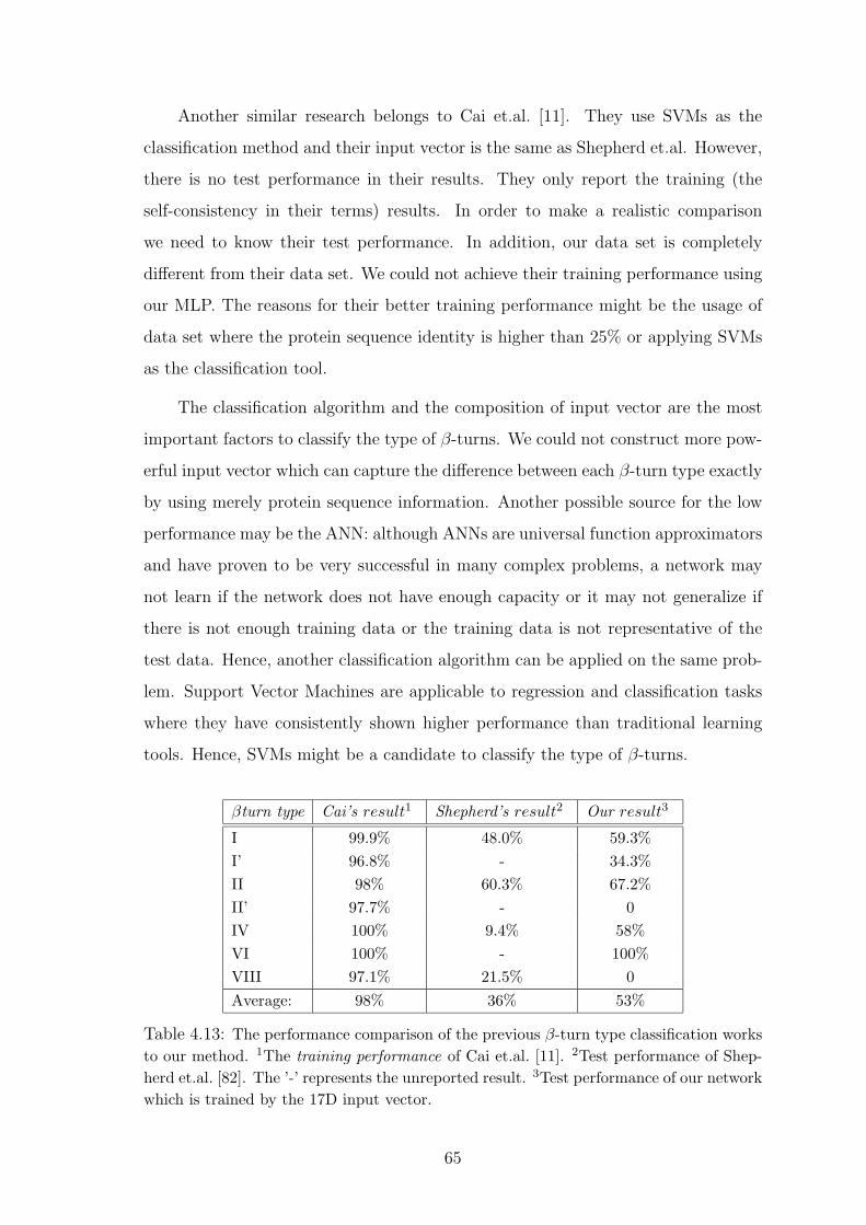
Another similar research belongs to Cai et.al. [11]. They use SVMs as the
classification method and their input vector is the same as Shepherd et.al. However,
there is no test performance in their results. They only report the training (the
self-consistency in their terms) results. In order to make a realistic comparison
we need to know their test performance. In addition, our data set is completely
different from their data set. We could not achieve their training performance using
our MLP. The reasons for their better training performance might be the usage of
data set where the protein sequence identity is higher than 25% or applying SVMs
as the classification tool.
The classification algorithm and the composition of input vector are the most
important factors to classify the type of β-turns. We could not construct more pow-
erful input vector which can capture the difference between each β-turn type exactly
by using merely protein sequence information. Another possible source for the low
performance may be the ANN: although ANNs are universal function approximators
and have proven to be very successful in many complex problems, a network may
not learn if the network does not have enough capacity or it may not generalize if
there is not enough training data or the training data is not representative of the
test data. Hence, another classification algorithm can be applied on the same prob-
lem. Support Vector Machines are applicable to regression and classification tasks
where they have consistently shown higher performance than traditional learning
tools. Hence, SVMs might be a candidate to classify the type of β-turns.
βturn type Cai’s result1 Shepherd’s result2 Our result3
I 99.9% 48.0% 59.3%I’ 96.8% - 34.3%II 98% 60.3% 67.2%II’ 97.7% - 0IV 100% 9.4% 58%VI 100% - 100%VIII 97.1% 21.5% 0Average: 98% 36% 53%
Table 4.13: The performance comparison of the previous β-turn type classification worksto our method. 1The training performance of Cai et.al. [11]. 2Test performance of Shep-herd et.al. [82]. The ’-’ represents the unreported result. 3Test performance of our networkwhich is trained by the 17D input vector.
65
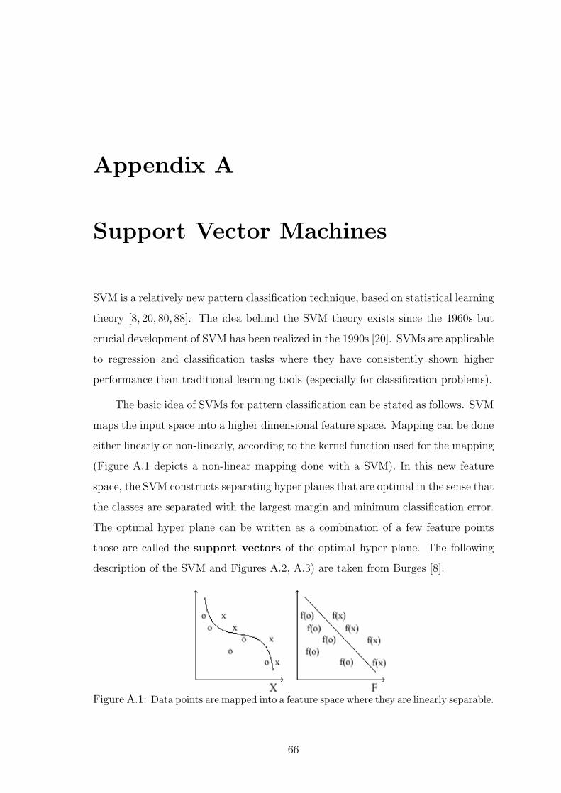
Appendix A
Support Vector Machines
SVM is a relatively new pattern classification technique, based on statistical learning
theory [8, 20, 80, 88]. The idea behind the SVM theory exists since the 1960s but
crucial development of SVM has been realized in the 1990s [20]. SVMs are applicable
to regression and classification tasks where they have consistently shown higher
performance than traditional learning tools (especially for classification problems).
The basic idea of SVMs for pattern classification can be stated as follows. SVM
maps the input space into a higher dimensional feature space. Mapping can be done
either linearly or non-linearly, according to the kernel function used for the mapping
(Figure A.1 depicts a non-linear mapping done with a SVM). In this new feature
space, the SVM constructs separating hyper planes that are optimal in the sense that
the classes are separated with the largest margin and minimum classification error.
The optimal hyper plane can be written as a combination of a few feature points
those are called the support vectors of the optimal hyper plane. The following
description of the SVM and Figures A.2, A.3) are taken from Burges [8].
Figure A.1: Data points are mapped into a feature space where they are linearly separable.
66
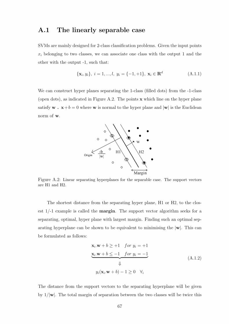
A.1 The linearly separable case
SVMs are mainly designed for 2-class classification problems. Given the input points
xi belonging to two classes, we can associate one class with the output 1 and the
other with the output -1, such that:
{xi, yi}, i = 1, ..., l, yi = {−1, +1}, xi ∈ Rd (A.1.1)
We can construct hyper planes separating the 1-class (filled dots) from the -1-class
(open dots), as indicated in Figure A.2. The points x which line on the hyper plane
satisfy w . x+b = 0 where w is normal to the hyper plane and |w| is the Euclidean
norm of w.
Figure A.2: Linear separating hyperplanes for the separable case. The support vectorsare H1 and H2.
The shortest distance from the separating hyper plane, H1 or H2, to the clos-
est 1/-1 example is called the margin. The support vector algorithm seeks for a
separating, optimal, hyper plane with largest margin. Finding such an optimal sep-
arating hyperplane can be shown to be equivalent to minimising the |w|. This can
be formulated as follows:
xi.w + b ≥ +1 for yi = +1
xi.w + b ≤ −1 for yi = −1︸ ︷︷ ︸⇓
yi(xi.w + b) − 1 ≥ 0 ∀i
(A.1.2)
The distance from the support vectors to the separating hyperplane will be given
by 1/|w|. The total margin of separation between the two classes will be twice this
67
distance 2/|w|. The aim is to maximise the margin of separation. Since this is given
by 2/|w|, it is clear that this is equivalent to minimization of the function subject
to the constraints yi(xi.w + b) ≥ 1 ∀i.
The constraint equations A.1.2 are multiplied by positive Lagrange multipliers
αi, i = 1, ..., l and subtracted from the objective function. This gives:
Lp ≡ 1
2||w||2 −
l∑i=1
αiyi(xi.w) + b +l∑
i=1
αi (A.1.3)
We want to minimize Lp with respect to w, b and maximize with respect to all the
αi. Now it is a convex quadratic programming problem. The gradient of Lp with
respect to w and b gives:
w =∑
i
αiyixi (A.1.4)
∑i
αiyi = 0 (A.1.5)
These are the equality constraints in the dual formulation, we substitute them into
equation A.1.3 and it gives:
LD =∑
i
αi − 1
2
∑i,j
αiαjyiyjxi.xj (A.1.6)
Support vector training maximizes LD with respect to the αi subject to constraints
A.1.5 with solution given by A.1.4. Those points for which αi > 0 lying on one of
the separating hyper planes H1 or H2, are called the support vectors. The support
vectors are the critical elements of the training set. They lie closest to the decision
boundary; if all other training points were removed and training was repeated, the
same separating hyperplane would be found.
The class label (positive or negative) of a new data point x is assigned by using
the decision function is generalized from equation A.1.4 such that :
F (x) = sign(w.x + b) = sign(Ns∑i=1
αiyi(xi.x) + b) (A.1.7)
where yi are the class labels; (.) indicates the inner product; b is the bias; Ns are
the set of support vectors; αi are the positive Lagrange multipliers.
68
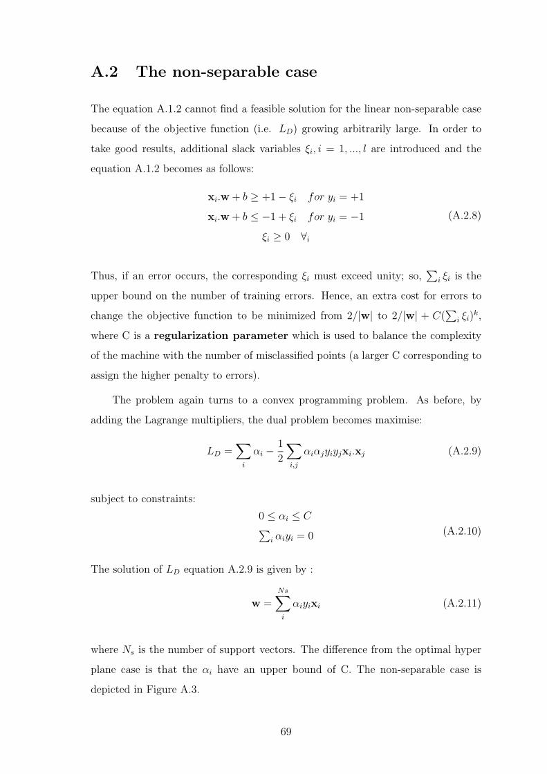
A.2 The non-separable case
The equation A.1.2 cannot find a feasible solution for the linear non-separable case
because of the objective function (i.e. LD) growing arbitrarily large. In order to
take good results, additional slack variables ξi, i = 1, ..., l are introduced and the
equation A.1.2 becomes as follows:
xi.w + b ≥ +1 − ξi for yi = +1
xi.w + b ≤ −1 + ξi for yi = −1
ξi ≥ 0 ∀i
(A.2.8)
Thus, if an error occurs, the corresponding ξi must exceed unity; so,∑
i ξi is the
upper bound on the number of training errors. Hence, an extra cost for errors to
change the objective function to be minimized from 2/|w| to 2/|w| + C(∑
i ξi)k,
where C is a regularization parameter which is used to balance the complexity
of the machine with the number of misclassified points (a larger C corresponding to
assign the higher penalty to errors).
The problem again turns to a convex programming problem. As before, by
adding the Lagrange multipliers, the dual problem becomes maximise:
LD =∑
i
αi − 1
2
∑i,j
αiαjyiyjxi.xj (A.2.9)
subject to constraints:
0 ≤ αi ≤ C∑i αiyi = 0 (A.2.10)
The solution of LD equation A.2.9 is given by :
w =Ns∑i
αiyixi (A.2.11)
where Ns is the number of support vectors. The difference from the optimal hyper
plane case is that the αi have an upper bound of C. The non-separable case is
depicted in Figure A.3.
69
Figure A.3: Linear separating hyperplanes for the non-separable case.
In the case of linearly non-separable data, one can use different kernel
functions to obtain better separation with linear hyper planes. The most commonly
used kernel functions are listed below:
Polynomial : K(x, y) = ((x.y) + θ)d
Gaussian : K(x, y) = exp(− ||x−y||22σ2 )
Sigmoid : K(x, y) = tanh((x.y) + θ)
70
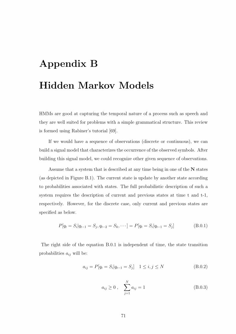
Appendix B
Hidden Markov Models
HMMs are good at capturing the temporal nature of a process such as speech and
they are well suited for problems with a simple grammatical structure. This review
is formed using Rabiner’s tutorial [69].
If we would have a sequence of observations (discrete or continuous), we can
build a signal model that characterizes the occurrence of the observed symbols. After
building this signal model, we could recognize other given sequence of observations.
Assume that a system that is described at any time being in one of the N states
(as depicted in Figure B.1). The current state is update by another state according
to probabilities associated with states. The full probabilistic description of such a
system requires the description of current and previous states at time t and t-1,
respectively. However, for the discrete case, only current and previous states are
specified as below.
P [qt = Si|qt−1 = Sj, qt−2 = Sk, · · · ] = P [qt = Si|qt−1 = Sj] (B.0.1)
The right side of the equation B.0.1 is independent of time, the state transition
probabilities aij will be:
aij = P [qt = Si|qt−1 = Sj] 1 ≤ i, j ≤ N (B.0.2)
aij ≥ 0 ,N∑
j=1
aij = 1 (B.0.3)
71
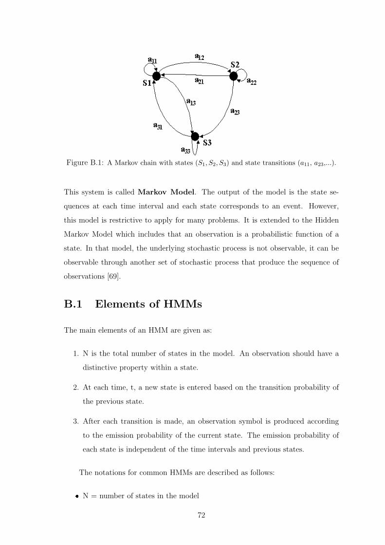
Figure B.1: A Markov chain with states (S1, S2, S3) and state transitions (a11, a23,...).
This system is called Markov Model. The output of the model is the state se-
quences at each time interval and each state corresponds to an event. However,
this model is restrictive to apply for many problems. It is extended to the Hidden
Markov Model which includes that an observation is a probabilistic function of a
state. In that model, the underlying stochastic process is not observable, it can be
observable through another set of stochastic process that produce the sequence of
observations [69].
B.1 Elements of HMMs
The main elements of an HMM are given as:
1. N is the total number of states in the model. An observation should have a
distinctive property within a state.
2. At each time, t, a new state is entered based on the transition probability of
the previous state.
3. After each transition is made, an observation symbol is produced according
to the emission probability of the current state. The emission probability of
each state is independent of the time intervals and previous states.
The notations for common HMMs are described as follows:
� N = number of states in the model
72
� M = number of distinct observation symbols
� T = length of the observation sequence
� Q = {q1, q2, · · · , qN} states
� V = {v1, v2, · · · , vM} discrete set of possible observation symbols
� A = {aij}, aij = P (qj at t + 1 | qi at t) state transition probability which is
the probability of being in state j at time t+1 given that it was in state i at
time t.
� B = {bj(k)}, bj(k) = P (vk at t | qj at t) observation (emission) symbol proba-
bility which is the probability of observing the symbol vk given that in state
j.
� π = {πi}, πi = P (qi at t = 1), initial state distribution which is the probability
of being in state i at the beginning at time t = 1.
� Ot denotes the observation symbol observed at time t.
Using the HMM an observation sequence O = O1, O2, · · · , OT , is generated as
follows: Choose an initial state, i1 according to the initial state probability πi, set the
time t=1, and choose an observation symbol O1 according to emission probability
distribution bi(k). After t becomes t+1, choose it+1 according to transition prob-
ability distribution at+1 and select observation symbol Ot+1 according to emission
probability distribution bj(k). Continue this procedure until reach time T.
The compact notation to represent an HMM is λ = (A,B, π).
B.2 The Three Problems for HMMs
There exist three crucial problems which must be solved for an HMM to use it in
applications.
1. Problem : Given the model λ = (A,B, π) how do we compute P (O|λ) that is
the probability of occurrence of the observation sequence O = O1, O2, · · · , OT .
73
Another explanation of first problem is that there is a given model and a
sequence of observations, so how we evaluate the model.
2. Problem : Given the model λ = (A,B, π) how do we choose a state sequence
I = i1, i2, · · · , iT , so that P (O, I|λ), the joint probability of the observation
sequence (O = O1, O2, · · · , OT ,) and state sequence (I) given the model (λ)
is maximized. That problem tries to find the hidden part of a model, state
sequence.
3. Problem : How we could adjust the HMM parameters λ = (A,B, π) so
that P (O|λ) is maximized. It optimizes the model parameters to describe the
observation sequence. These parameters are used in the training of the model.
B.2.1 Solution to the First Problem
The aim is to calculate the probability of the observation sequence given the model.
The easiest way of doing that to enumerate every possible state sequence. For a
fixed state sequence I = i1, i2, · · · , iT ,, the probability of the observation sequence
O is:
P (O|I, λ) = bi1(O1)bi2(O2) · · · biT (OT ) (B.2.4)
The probability of a state sequence I is:
P (I|λ) = πi1ai1i2ai2i3 · · · aiT−1iT (B.2.5)
The joint probability of O and I is the multiplication of the probabilities in equations
B.2.4 and B.2.5.
P (O, I|λ) = P (O|I, λ) P (I|λ) (B.2.6)
The probability of O that given model λ can be calculated using summation of the
joint probability (P (O, I|λ)) over all possible state sequences (I) :
P (O|λ) =∑
I
P (O|I, λ)P (I|λ) =∑
i1,i2,...,iT
πi1bi1(O1)ai1i2bi2(O2) · · · aiT−1iT biT (OT )
(B.2.7)
74
In equation B.2.7, the multiplications require 2T-1 computations. All possible state
sequences are NT . So, it requires the 2T.NT multiplications, it is hugh computa-
tions. Therefore, another method, forward-backward procedures, was developed
to solve this problem.
B.2.1.1 Forward Procedure
Assume that a forward variable αt(i) is defined as follows:
αt(i) = P (O1, O2, · · · , OT , it = qi|λ) (B.2.8)
The probability of the partial observation sequence up to time t and the state qi at
time t given the model λ. The αt(i) is computed as follows:
1. Initialization:
αt(i) = πi.bi(O1) ; 1 ≤ i ≤ N (B.2.9)
It initiates the forward probabilities as the joint probability of state qi and
initial observation O1.
2. Induction:
for t = 1, 2, · · · , T − 1 ; 1 ≤ j ≤ N
αt+1(j) =
[ N∑i=1
αiaij
]bj(Ot+1) (B.2.10)
Figure B.2 depicts that how state qj is reached at time t+1 from N possible of
states, qi, at time t. The αt(i) is the probability of joint event (O1, O2, · · · , Ot)
and states qi stops at time t. The product of αiaij is the probability of the
joint event (O1, O2, · · · , Ot) and state qj reaches at time t+1. The summation
of this product over all possible N states for qi includes previous observations.
After that computation is performed and Sj is known, the αt+1(j) is computed
by multiplying the summed quantity with the emission probability bj(Ot+1).
75
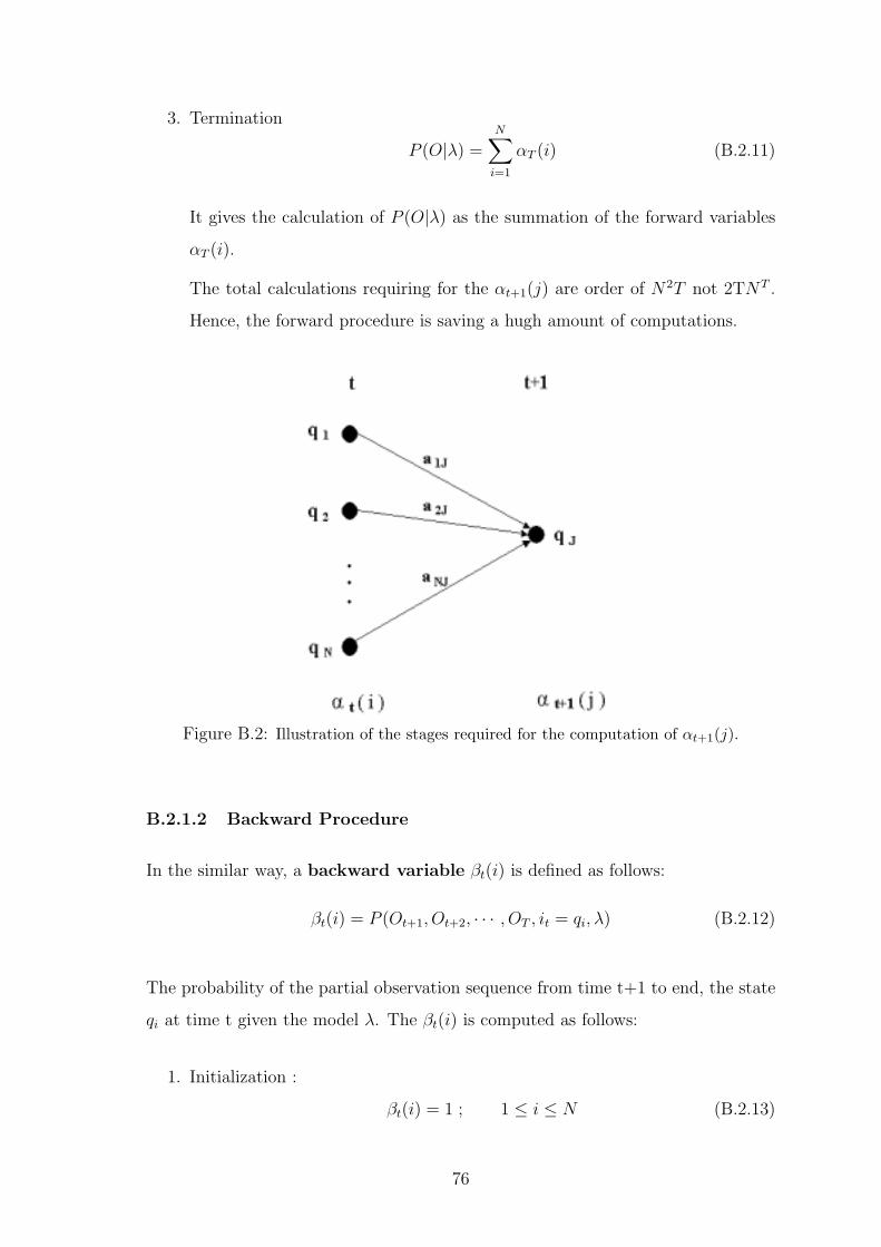
3. Termination
P (O|λ) =N∑
i=1
αT (i) (B.2.11)
It gives the calculation of P (O|λ) as the summation of the forward variables
αT (i).
The total calculations requiring for the αt+1(j) are order of N2T not 2TNT .
Hence, the forward procedure is saving a hugh amount of computations.
Figure B.2: Illustration of the stages required for the computation of αt+1(j).
B.2.1.2 Backward Procedure
In the similar way, a backward variable βt(i) is defined as follows:
βt(i) = P (Ot+1, Ot+2, · · · , OT , it = qi, λ) (B.2.12)
The probability of the partial observation sequence from time t+1 to end, the state
qi at time t given the model λ. The βt(i) is computed as follows:
1. Initialization :
βt(i) = 1 ; 1 ≤ i ≤ N (B.2.13)
76
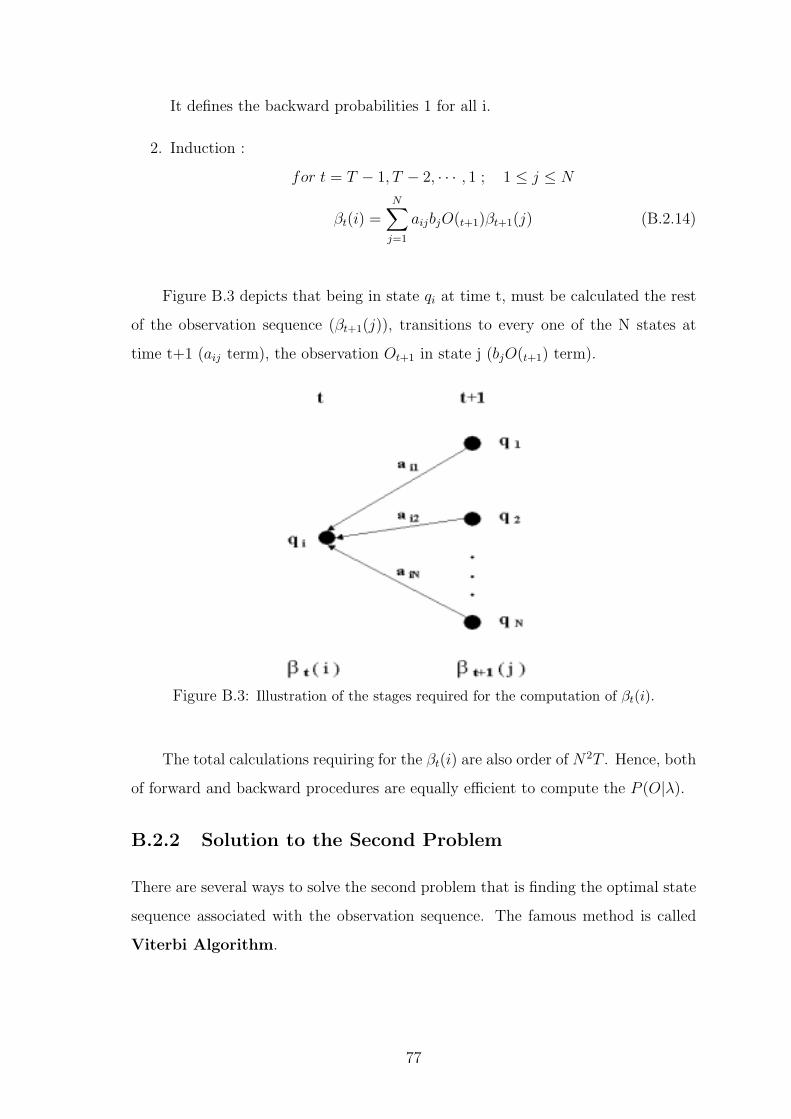
It defines the backward probabilities 1 for all i.
2. Induction :
for t = T − 1, T − 2, · · · , 1 ; 1 ≤ j ≤ N
βt(i) =N∑
j=1
aijbjO(t+1)βt+1(j) (B.2.14)
Figure B.3 depicts that being in state qi at time t, must be calculated the rest
of the observation sequence (βt+1(j)), transitions to every one of the N states at
time t+1 (aij term), the observation Ot+1 in state j (bjO(t+1) term).
Figure B.3: Illustration of the stages required for the computation of βt(i).
The total calculations requiring for the βt(i) are also order of N2T . Hence, both
of forward and backward procedures are equally efficient to compute the P (O|λ).
B.2.2 Solution to the Second Problem
There are several ways to solve the second problem that is finding the optimal state
sequence associated with the observation sequence. The famous method is called
Viterbi Algorithm.
77
B.2.2.1 Viterbi Algorithm
It is an inductive algorithm, a kind of dynamic algorithm, at each instant the best
(with maximum probability) possible state sequence is kept. In this way we finally
have the best path for each of N states as the last state for the desired observation
sequence. Then we choose the one with the highest probability.
In order to find best state sequence (Q =q1q2 · · · qt) for the given observation
sequence (O =O1O2 · · ·OT ), a quantity is defined: δt(i) is the best score along
a single path, it accounts for the first t observation and stops in state qi. The
definition of δt(i) is:
δt(i) = maxq1q2···qt−1
P [q1q2 · · · qt = i, O1O2 · · ·OT |λ] (B.2.15)
We calculate δt+1(j) by induction such as:
δt+1(j) = [maxi
δt(i)aij]bj(Ot+1) (B.2.16)
We should keep the track of the argument maximized (eq. B.2.16) for each t and j,
to retrieve the state sequence later. The storage ψt(j) is used for that purpose. The
formal steps to find the best state sequence are given below :
1. Initialization :
δ1(i) = πibi(O1) 1 ≤ i ≤ N
ψ1(i) = 0 (B.2.17)
2. Recursion :
δt(j) = max1≤i≤N
[δt−1(i)aij] bj(Ot) 2 ≤ t ≤ T ; 1 ≤ j ≤ N (B.2.18)
ψt(j) = arg max1≤i≤N
[δt−1(i)aij] 2 ≤ t ≤ T ; 1 ≤ j ≤ N (B.2.19)
3. Termination :
P ∗ = max1≤i≤N
[δT (i)] (B.2.20)
q∗T = arg max1≤i≤N
[δT (i)] (B.2.21)
78
4. State sequence backtracking :
q∗t = ψt+1(q∗t+1) t = T − 1, T − 2, · · · , 1 (B.2.22)
The Viterbi algorithm is very similar to forward-backward procedure except for
the comparisons required to find the maximum value. The complexity of Viterbi
algorithm is also the order of N2T .
B.2.3 Solution to the Third Problem
The last problem deals with the determination of the model training parameters. It
optimizes the model parameters (A, B, π) to make the maximum the probability of
observation sequence. We will choose these parameters (A, B, π) using an iterative
process such as Baum-Welch method.
B.2.3.1 Baum-Welch Algorithm
It adjusts the model parameters to increase P (O|λ). The calculation of P (O|λ) is
the summation of P (O, I|λ) over all possible state sequence (I). However, we should
make this optimization for all states sequences not a given one to solve the third
problem.
Baum-Welch Algorithm takes an initial model that is improved until P (O|λ)
becomes maximum. So, we assume that there is an initial HMM at the beginning.
Then a probability, ξt(i, j), is defined as:
ξt(i, j) = P [it = qt|it+1 = qj|O, λ] (B.2.23)
It is the probability of a being in state qi at time t and going to state qj at time
t+1, given the observation sequence (O) and model (λ). By using equations in
forward-backward procedures, ξt(i, j) is written as :
ξt(i, j) =αt(i) aij bj (Ot+1) βt+1(j)
P [O|λ](B.2.24)
79
where αt(i) accounts for the observations O1, O2, · · · , Ot; aij accounts for the tran-
sition to state j; bj (Ot+1) picks up the symbol Ot+1 from state j; βt+1(j) accounts
for the remaining observation sequences Ot+2, Ot+3, · · · , OT .
Now, we define a new variable, γt(i), which is the probability of being state qi
at time t, given the observation sequence and the model:
γt(i) = P (it = qi|O, λ) (B.2.25)
Using Bayes law and forward-backward procedure, γt(i) can be written as:
γt(i) =P (it = qi, O|λ)
P (O|λ)=
αt(i) βt(i)
P (O|λ)(B.2.26)
If we consider the equations B.2.24 and B.2.26, the summation of ξt(i, j) over all j
gives the γt(i) as follows:
γt(i) =N∑
j=1
ξt(i, j) (B.2.27)
The summation of γt(i) from t = 1 to T gives the expected number of times that
state qi is visited. Similarity, the summation of γt(i) from t = 1 to T − 1 gives the
expected number of transitions made from state qi. The summation of ξt(i, j) from
t = 1 to T − 1 gives the expected number of transitions from state qi to qj. So,
T−1∑t=1
γt(i) = Expected number of transitions made from state qi (B.2.28)
T−1∑t=1
ξt(i, j) = Expected number of transitions from state qi to qj (B.2.29)
The Baum-Welch re-estimation formulas are presented using above equations:
πi = γ1(i) (B.2.30)
aij =T−1∑t=1
ξt(i, j)
/T−1∑t=1
γt(i) (B.2.31)
¯bj(k) =T∑t=1
Ot=k
γt(j)
/T∑
t=1
γt(j) (B.2.32)
80
The re-estimation formula for πi is the probability of being in state qi at time t=1.
The formula for aij is the ratio of expected number of making transitions from state
qi to state qj divided by the expected number of making transitions out of state qi.
The formula for bj(k) is the ratio of the expected number of times of being in state
qj, observing symbol Ok divided by the expected number of times being in state qj.
The summation for bj(k) goes from t=1 up to t=T.
The initial model is λ and the re-estimation model is λ which consists of the
above parameters πi , aij , ¯bj(k), then it can be shown that either :
1. The initial model λ is a critical point of the likelihood function in which case
λ = λ or,
2. P (O|λ) > P (O|λ), found a better model λ from which the observation se-
quence is more likely to be produced.
If λ is used in place of λ iteratively and repeated the re-estimation, we could
improve the probability of O being observed form the model. The final result of the
re-estimation operation is called maximum likelihood estimate of the HMM.
81
Appendix C
Artificial Neural Networks
The neurons are found in the human brain that are many and varied. Artificial
neurons are simplified models based on the known properties of biological neurons.
The Artificial Neural Network (ANN) is a parallel dynamical system consisting of
multiple simple units that can perform transformations by their state response to
their input information.
Over the last decade, many different ANN models have been proposed for broad
range of applications. For supervised classification tasks, the multilayer feedforward
neural network (MLP) and the learning vector quantisation (LVQ) network are the
most commonly used models.
The multi-layer perceptron came into favor when Rumelhart et.al. applied
the gradient backpropagation algorithm for training layered networks of perceptron
elements [78]. The LVQ method was developed by Kohonen who also developed
the popular unsupervised classification technique known as the self-organising map
neural networks [47].
C.1 The Artificial Neuron
An artificial neuron computes a function of a weighted sum of inputs:
y = f(a) = f(n∑i
xiwi − b) (C.1.1)
where xi input, each input has an associated wi weight, b is a threshold value to be
activated or not. The illustration of a neuron is given in Figure C.1.
82
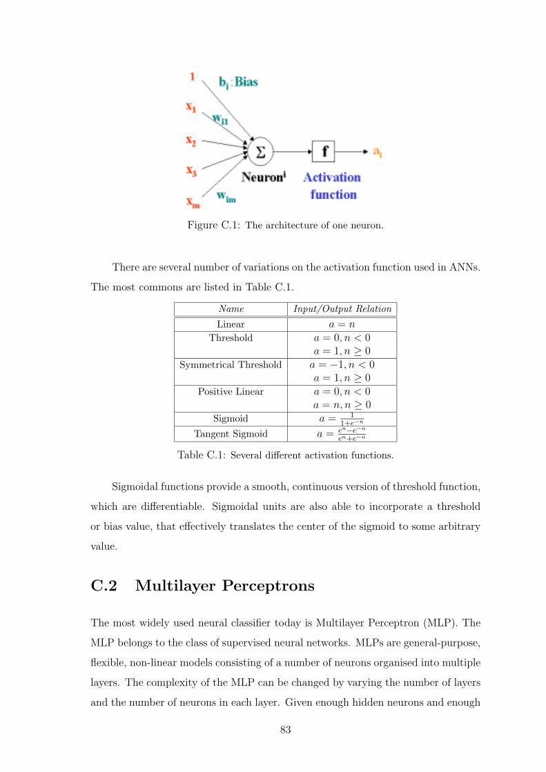
Figure C.1: The architecture of one neuron.
There are several number of variations on the activation function used in ANNs.
The most commons are listed in Table C.1.
Name Input/Output Relation
Linear a = nThreshold a = 0, n < 0
a = 1, n ≥ 0Symmetrical Threshold a = −1, n < 0
a = 1, n ≥ 0Positive Linear a = 0, n < 0
a = n, n ≥ 0Sigmoid a = 1
1+e−n
Tangent Sigmoid a = en−e−n
en+e−n
Table C.1: Several different activation functions.
Sigmoidal functions provide a smooth, continuous version of threshold function,
which are differentiable. Sigmoidal units are also able to incorporate a threshold
or bias value, that effectively translates the center of the sigmoid to some arbitrary
value.
C.2 Multilayer Perceptrons
The most widely used neural classifier today is Multilayer Perceptron (MLP). The
MLP belongs to the class of supervised neural networks. MLPs are general-purpose,
flexible, non-linear models consisting of a number of neurons organised into multiple
layers. The complexity of the MLP can be changed by varying the number of layers
and the number of neurons in each layer. Given enough hidden neurons and enough
83
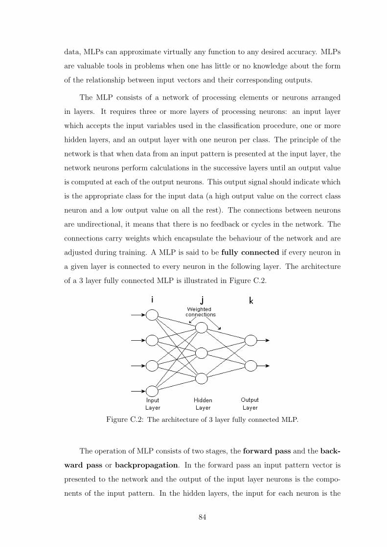
data, MLPs can approximate virtually any function to any desired accuracy. MLPs
are valuable tools in problems when one has little or no knowledge about the form
of the relationship between input vectors and their corresponding outputs.
The MLP consists of a network of processing elements or neurons arranged
in layers. It requires three or more layers of processing neurons: an input layer
which accepts the input variables used in the classification procedure, one or more
hidden layers, and an output layer with one neuron per class. The principle of the
network is that when data from an input pattern is presented at the input layer, the
network neurons perform calculations in the successive layers until an output value
is computed at each of the output neurons. This output signal should indicate which
is the appropriate class for the input data (a high output value on the correct class
neuron and a low output value on all the rest). The connections between neurons
are undirectional, it means that there is no feedback or cycles in the network. The
connections carry weights which encapsulate the behaviour of the network and are
adjusted during training. A MLP is said to be fully connected if every neuron in
a given layer is connected to every neuron in the following layer. The architecture
of a 3 layer fully connected MLP is illustrated in Figure C.2.
Figure C.2: The architecture of 3 layer fully connected MLP.
The operation of MLP consists of two stages, the forward pass and the back-
ward pass or backpropagation. In the forward pass an input pattern vector is
presented to the network and the output of the input layer neurons is the compo-
nents of the input pattern. In the hidden layers, the input for each neuron is the
84
sum of the scalar products of the incoming vector components with their respective
weights. The input of a neuron j is given by:
inputj =n∑i
wjiouti (C.2.2)
where wji is the weight connecting neuron i to neuron j and outi is the output of
neuron i. The output of neuron j is given by:
outj = f(inputj) (C.2.3)
The function f denotes the activation function of each neuron. The output of a
neuron is sent to all neurons in the following layer. It will continue through all
the layers until the output layer is reached. The input layer neurons just take the
corresponding value from the input pattern vector.
The MLP is trained by supervised learning using the iterative backpropagation
algorithm. In the learning phase, the training set patterns are presented at the input
layer as feature vectors, together with their corresponding desired output (target)
pattern which represents the classification for the input pattern. The training starts
with small random weights. For each input pattern the network is required to
adjust the weights attached to the connections so that the difference between the
network’s output and the target for that input pattern is decreased. The weights
between the output layer and the below hidden layer are adjusted by the generalised
delta rule [78]:
wkj(t + 1) = wkj(t) + η(δk outk) (C.2.4)
where wkj(t + 1) and wkj(t) are the weights connecting neurons j and k at iteration
(t+1) and t, respectively, η is a learning rate parameter. The δ for the hidden layer
neurons are calculated and the weights connecting the hidden layer with the layer
below are updated. This procedure is repeated until the last layer of weights has
been adjusted. Section C.2.1 shows how the generalised delta rule and δ are derived.
85
C.2.1 Backpropagation Algorithm
The backpropagation algorithm is a gradient descent optimisation procedure which
minimises the mean square error between the network’s output and the target
for all input patterns N.
E =1
2N
∑p
∑k
(targetk − outk)2 (C.2.5)
The training set is presented iteratively to the network until a stable set of weights
is achieved and the error function is reduced to an acceptable level. It is done by a
series of gradient descent weight updates:
∆wkj = −η∂Ep
∂wkj
(C.2.6)
where Ep is the mean squared error for input pattern p and is given by:
Ep =1
2
∑p
(targetk − outk)2 (C.2.7)
Using the chain rule the right hand side term of equation C.2.6 can be written as
follows:
− ∂Ep
∂wkj
= − ∂Ep
∂ inputk
∂ inputk∂wkj
(C.2.8)
The weight changes can be expressed as the product of two terms; the rate of change
of error with respect to the input to neuron k and the change of the input to neuron
k with respect to a change in the weight between neurons j and k. If we apply the
equation C.2.2 to the second part of equation C.2.8 :
∂ inputk∂wkj
=∂
∑wkjoutj
∂wkj
= outj (C.2.9)
We define δk as :
δk = − ∂Ep
∂ inputk(C.2.10)
We substitute the equations C.2.9 and C.2.10 in equation C.2.6 :
∆wkj = −ηδkoutj (C.2.11)
86
If we use the chain rule, we can express δk in terms of the rate of change of error
with respect to the output of neuron k and the change of the output of neuron k
with respect to the input to the neuron k as follows:
δk = − ∂Ep
∂ inputk= − ∂Ep
∂outk
∂outk∂ inputk
(C.2.12)
Using equation C.2.3 we get :
∂outk∂ inputk
= f ′(inputk) (C.2.13)
Using equation C.2.7 we get :
∂Ep
∂outk= −(targetk − outk) (C.2.14)
When we substitute the equations C.2.13 and C.2.14 in equation C.2.10, we get the
δ for an output neuron k as follows:
δk = (targetk − outk) f ′(inputk) (C.2.15)
Finally if we substitute equation C.2.15 in equation C.2.11, we get:
∆wkj = −η (targetk − outk) f ′(inputk) outj (C.2.16)
If we have a neuron j which is in the hidden layer, we use chain rule to get δj :
δj = f ′(inputj)∑
k
δkwkj (C.2.17)
The weight update of that neuron j will be :
∆wji = −η f ′(inputj)∑
k
δkwkj outi (C.2.18)
The equations C.2.18 and C.2.16 are the weight update rules for the hidden and the
output layers, respectively.
If we update the weights after each training pattern, rather than adding up the
weight changes for all the patterns before applying them, the learning algorithm is
87
no longer true gradient descent. It is called online learning. If we keep the step
sizes (η) small enough, the erratic behaviour of the weight updates will not be too
much of a problem, and the increased number of weight changes will still get us to
the minimum quicker than true gradient descent. It is called batch learning.
The training steps of a fully connected MLP is given below:
1. Take the set of N training patterns to learn
2. Set up the network with i input units fully connected to j hidden units via
connections with weights wji, which in turn are fully connected to k output
units via connections with weights wkj
3. Generate random initial weights
4. Select an appropriate error function E(wkj) and learning rate η
5. Apply the weight update equation ∆wkj = −η∂E(wkj)
∂wkjto each weight wkj for
each training pattern p. One set of updates of all the weights for all the
training patterns is called one epoch of training
6. Repeat step 5 until the network error function is small enough.
C.3 Heuristics for MLPs
Several number of heuristics are developed to use in training a MLP. Some of them
are widely considered to be very useful for improving the training speed and quality
of solution reached by training algorithms.
1. Initialization of weight values: The weights in a MLP should be initialized to
small, random values prior to training. The performance of backpropagation
and other algorithms can be highly dependent on the initialization of weights.
The general heuristic commonly used is to initialize weights such that the
sigmoidal activation functions in the network operate in their linear range
(very small weights however result in very small gradient values).
2. Pre-processing of training data: The pre-processing includes the dimensional-
ity reduction techniques which attempt to reduce the number of inputs without
88
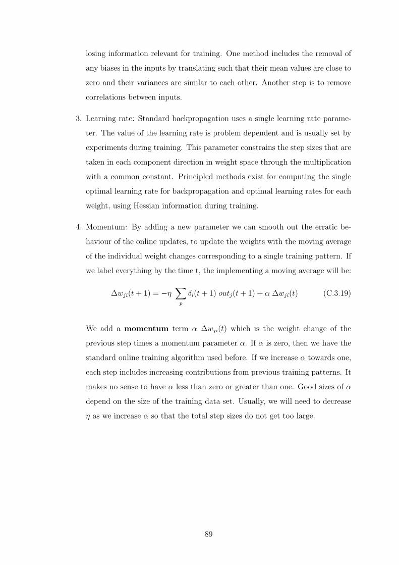
losing information relevant for training. One method includes the removal of
any biases in the inputs by translating such that their mean values are close to
zero and their variances are similar to each other. Another step is to remove
correlations between inputs.
3. Learning rate: Standard backpropagation uses a single learning rate parame-
ter. The value of the learning rate is problem dependent and is usually set by
experiments during training. This parameter constrains the step sizes that are
taken in each component direction in weight space through the multiplication
with a common constant. Principled methods exist for computing the single
optimal learning rate for backpropagation and optimal learning rates for each
weight, using Hessian information during training.
4. Momentum: By adding a new parameter we can smooth out the erratic be-
haviour of the online updates, to update the weights with the moving average
of the individual weight changes corresponding to a single training pattern. If
we label everything by the time t, the implementing a moving average will be:
∆wji(t + 1) = −η∑
p
δi(t + 1) outj(t + 1) + α ∆wji(t) (C.3.19)
We add a momentum term α ∆wji(t) which is the weight change of the
previous step times a momentum parameter α. If α is zero, then we have the
standard online training algorithm used before. If we increase α towards one,
each step includes increasing contributions from previous training patterns. It
makes no sense to have α less than zero or greater than one. Good sizes of α
depend on the size of the training data set. Usually, we will need to decrease
η as we increase α so that the total step sizes do not get too large.
89
Bibliography
[1] Altschul, S., Madden, T., Shaffer, A., Zhang, J., Zhang, Z. Gapped Blast and PSI-Blast: a new generation of protein database search programs. Nucl. Acids Res. 25,3389-3402, 1997
[2] Bahar, I., Atilgan, A. R., Jernigan, R. L., Erman, B. Understanding the recognitionof protein structural classes by amino acid composition. Proteins, 29(2), 172-185,1997
[3] Baldi, P., Brunak, S., Frasconi, P., Soda, G., Pollastri, G. Exploiting the past andthe future in protein secondary structure prediction. Bioinformatics, 15, 937-946,1999
[4] Baysal, C., Atilgan, A. R. Coordination Topology and Stability for the Native andBinding Conformers of Chymotrypsin Inhibitor 2. Proteins, 45, 62-70, 2001
[5] Berman, H. M., Westbrook, J., Feng, Z., Gilliland, G., Bhat, T. N., Weissig, H.,Shindyalov, I. N., Bourne, P. E. The Protein Data Bank. Nucleic Acids Res. 28(1),235-242, 2000
[6] Blout, E. R. The dependence of the conformation of polypeptides and proteinsupon amino acid composition. Polyamino Acids, Polypeptides, and Proteins, 275-279, 1962
[7] Bryant, S.H. Evaluation of threading specificity and accuracy. Proteins: Struct.Funct. Genet. 26, 172-185, 1996
[8] Burges, C.J. C. A Tutorial on Support Vector Machines for Pattern Recognition.Data Mining and Knowledge Discovery, 2, 121-167, 1998
[9] Cai, Y., Zhou, G. Prediction of protein structural classes by neural network.Biochem. 82(8), 783-787, 2000
[10] Cai, Y. D., Liu, X. J., Xu, Xb., Chou, K. C. Prediction of protein structural classesby Support Vector Machines. Comput. Chem. 26(3), 293-296, 2002
[11] Cai, D. Y., Liu X. J., Xu, X. B., Chou, K. C. Support Vector Machines for theclassification and prediction of β-turn types. J. Pept. Sci. 8, 297-301, 2002
[12] Chandonia, J. M., Karplus, M. Neural networks for secondary structure and struc-tural class predictions. Protein Sci. 4(2), 275-285, 1995
[13] Chang, C. C., Lin, C. J. LIBSVM: a Library for Support Vector Machines. Ver-sion=2.33, 2002
90
[14] Chou, K. C. A novel approach to predicting protein structural classes in a (20-1)-Damino acid composition space. Proteins, 21(4), 319-344, 1995
[15] Chou, K. C. Prediction and classification of β-turn types. Biopolymers, 42, 837-853,1997
[16] Chou, K. C. Prediction of tight turns and their types in proteins. Analy. Biochem.286, 1-16, 2000
[17] Chou, K. C. A key driving force in determination of protein structural classes.Biochem. Biophys. Res. Commun. 264(1), 216-224, 1999
[18] Chou, P. Y., Fasman, G. D. Prediction of protein conformation. Biochemistry, 13,222-245, 1974
[19] Chou, P. Y. Prediction of protein structural classes from amino acid composition.Prediction of protein structure and the principles of protein conformation(E. Fas-man, G. D.), Plenum Press, New York, 549-586, 1989
[20] Cristianini, N., Scholkopf, B. Support Vector Machines and Kernel Methods, TheNew Generation of Learning Machines. AI Magazine, 23(3), 31-41, 2002
[21] Cuff, J. A., Barton, G. J. Application of multiple sequence alignment profiles toimprove protein secondary structure prediction. Proteins, 40, 502-511, 2000
[22] Deleage, G., Dixon, J.S. Use of class prediction to improve protein secondary struc-ture prediction. Prediction of protein structure and the principles of protein confor-mation (E. Fasman, G. D.), Plenum Press, New York, 587-597, 1989
[23] Di Francesco, V., Garnier, J., Munson, P. J. Improving protein secondary structureprediction with aligned homologous sequences. Prot. Sci. 5, 106-113, 1996
[24] Ding, C. H., Dubchak, I. Multi-class protein fold recognition using support vectormachines and neural networks. Bioinformatics, 17(4), 349-358, 2001
[25] Eddy, S. R. Profile hidden Markov models. Bioinformatics,14, 755-763, 1998
[26] Eisenhaber, F., Persson, B., Argos, P. Protein structure prediction: recognition ofprimary, secondary, and tertiary structural features from amino acid sequence. Crit.Rev. Biochem. Mol. Biol. 30(1), 1-94, 1995
[27] Frishman, D., Argos, P. 75% accuracy in protein secondary structure prediction.Proteins, 27, 329-335, 1997
[28] ftp://ftp.embl-heidelberg.de/pub/databases/protein extras/pdb select
[29] Higgins, D. G., Thompson, J. D., Gibson, T. J. Using CLUSTAL for multiplesequence alignments. Meth. Enzymol. 266, 383-402, 1996
[30] Hobohm, U., Sander, C. Enlarged representative set of protein structures. ProteinSci. 3, 522, 1994
[31] Holley, H., Karplus, M. Protein secondary structure prediction with a neural net-work. Proceedings of the National Academy of Science of the United States of Amer-ica, 86, 152-156, 1989
[32] http://htk.eng.cam.ac.uk/
91
[33] Hughey, R., Krogh, A. Hidden Markov models for sequence analysis: extension andanalysis of the basic method. CABIOS, 12, 95-107, 1996
[34] Hutchinson, E. G., Thornton, J. M. A revised set of potentials for β-turn formationin proteins. Protein Sci. 3, 22072216, 1994
[35] Hutchinson, E. G. and Thornton, J. M. PROMOTIF - a program to identify andanalyze structural motifs in proteins. Protein Sci. 5, 212-220, 1996
[36] Islamaj, Rezerta. Two or three dimensional representation of amino acid character-istics. 2000
[37] Jones, D. T., Taylor, W. R., Thornton, J. M. A new approach to protein foldrecognition. Nature, 358, 86-89, 1992
[38] Jones, D. T. GenThreader: An efficient and reliable protein fold recognition methodfor genomic sequences. J. Mol. Biol. 287, 797-815, 1999
[39] Jones, D. T. Protein secondary structure prediction based on position-specific scor-ing matrices. J. Mol. Biol. 292, 195-202, 1999
[40] Kabsch, W., Sander, C. Dictionary of protein secondary structure: pattern recogni-tion of hydrogen-bonded and geometrical features. Biopolymers, 22(12), 2577-2637,1983
[41] Karplus, K., Barrett, C., Hughey, R. Hidden Markov models for detecting remoteprotein homologies. Bioinformatics, 14, 846-856, 1998
[42] Karplus, K., Barrett, C., Cline, M., Diekhans, M., Grate, L. Predicting proteinstructure using only sequence information. Proteins, S3, 121-125, 1999
[43] Kaur, H., Raghava, G.P.S. Prediction of β-turns in proteins from multiple alignmentusing neural network. Protein Science, 12, 627-634, 2003
[44] King, R. D., Sternberg, M. J. Identification and application of the concepts impor-tant for accurate and reliable protein secondary structure prediction. Prot. Sci. 5,2298-2310, 1996
[45] Klein, P., Delisi, C. Prediction of protein structural class from the amino acidsequence. Biopolymers, 25(9), 1659-1672, 1986
[46] Kneller, D., Cohen, F. Improvements in secondary structure prediction by an en-hanced neural network. J. Mol. Biol. 214, 171-182, 1990
[47] Kohonen, T. Selforganized formation of topologically correct feature maps. Biolog-ical Cybernetics, 43, 59-69, 1982
[48] Lathrop, R. H., Smith, T. F. Global optimum protein threading with gapped align-ment and empirical pair score functions. J. Mol. Biol. 255, 641-665, 1996
[49] Lehninger, A. L., Nelson, D. L., Cox, M. M. Lehninger Principles of Biochemistry.Third Edition
[50] Leslie, C., Eskin, E., Noble, W. S. The Spectrum Kernel: A String Kernel For SVMProtein Classification. Pacific Symposium on Biocomputing, Hawaii, USA, 2002
92
[51] Levin, J. M., Pascarella, S., Argos, P., Garnier, J.Quantification of secondary struc-ture prediction improvement using multiple alignment. Prot. Engin. 6, 849-854,1993
[52] Levitt, M., Chothia, C. Structural patterns in globular proteins. Nature, 261(5561),552-558, 1976
[53] Lewis, P. N., Momany, F. A., Scheraga, H. A. Chain reversals in proteins. Biochim.Biophys. Acta. 303, 211-229, 1973
[54] Maclin, R., Shalvik, J. Using knowledge-based neural networks to improve algo-rithms: refining the chou-fasman algorithm for protein folding. Machine Learning,11, 195-215, 1993
[55] Mahalanobis, P. C. On the generalized distance in statistics. Proc. Natl. Inst. Sci.,Plenum Press,India, 2, 49-55, 1936
[56] Marti-Renom, M.A., Stuart, A., Fiser, A., Sanchez, R., Melo, F., Sali, A. Compara-tive protein structure modeling of genes and genomes. Annu. Rev. Biophys. Biomol.Struct. 29, 291-325, 2000
[57] Maxfield, F. R., Scheraga, H. A. Improvements in the Prediction of Protein Topog-raphy by Reduction of Statistical Errors. Biochem. 18, 697-704, 1979
[58] McGregor, M. J., Flores, T. P., Sternberg, M. J. E. Prediction of β-turns in proteinsusing neural networks. Protein Eng. 2(7), 521-526, 1989
[59] Mehta, P. K., Heringa, J., Argos, P. A simple and fast approach to prediction ofprotein secondary structure from multiply aligned sequences with accuracy above70
[60] Metfessel, B. A., Saurugger, P. N., Connelly, D. P., Rich, S. S. Cross-validation ofprotein structural class prediction using statistical clustering and neural networks.Protein Sci. 2(7), 1171-1182, 1993
[61] Mount, D.W., Bioinformatics and genome analysis, Cold Spring Harbor Press, 1999
[62] Murzin, A. G., Brenner, S. E., Hubbard, T., Chothia, C. SCOP: a structural clas-sification of proteins database for the investigation of sequences and structures. J.Mol. Biol. 247, 536-540, 1995
[63] Nakashima, H., Nishikawa, K., Ooi, T. The folding type of a protein is relevant tothe amino acid composition. J. Biochem. 99(1), 153-162, 1986
[64] Orengo, C. A., Taylor, W. R. SSAP: Sequential structure alignment program forprotein structure comparison. Meth. Enzymol. 266, 617-635, 1996
[65] Orengo,C.A., Todd, A., Thornton, J.M. From Protein Structure to Function. Curr.Op. in Str. Biol. 9, 374-382, 1999
[66] Pauling, L., Corey, R. B., Branson, H. R. The structure of proteins: Two hydrogen-bonded helical configurations of the polypeptide chain. Proc. Natl. Acad. Sci. U.S.A.37, 205-234, 1951
93
[67] Pearl, F. M. G, Lee, D., Bray, J. E., Sillitoe, I., Todd, A. E., Harrison, A. P.,Thornton, J. M., Orengo, C. A. Assigning genomic sequences to CATH NucleicAcids Research. 28(1), 277-282, 2000
[68] Qian, N., Sejnowski, T. Predicting the secondary structure of globular proteinsusing neural network models. J. Mol. Biol. 202, 865- 884, 1988
[69] Rabiner, L. R., Juang, B. H. An introduction to hidden markov models. IEEEMagazine on Accoustics, Speech and Signal Processing, 3(1), 4-16, 1986
[70] Richardson, J. S. The anatomy and taxonomy of protein structure. Adv. ProteinChem. 34, 167339, 1981
[71] Richardson, J. S. Richardson, D. C., Principles and patterns of protein conforma-tion. Prediction of protein structure and the principles of protein conformation(E.Fasman, G. D.), Plenum Press, New York, 1-98, 1989
[72] Riis, S. K., Krogh, A. Improving prediction of protein secondary structure usingstructured neural networks and multiple sequence alignments. J. Comp. Biol. 3,163-183, 1996
[73] Rose, G. D., Gierasch, L. M., Smith, J. A. Turns in peptides and proteins. Adv.Protein Chem. 37, 1109, 1985
[74] Rost, B., Sander, C. 1D secondary structure prediction through evolutionary pro-files. In Protein Structure by Distance Analysis (Bohr, H., Brunak, S., eds.), 257-276, IOS Press, Amsterdam, Oxford, Washington, 1994
[75] Rost, B. PHD: predicting one-dimensional protein structure by profile based neuralnetworks. Meth. Enzymol. 266, 525-539, 1996
[76] Rost, B. Better secondary structure prediction through more data. Columbia Uni-versity, 2000, http://cubic.bioc.columbia.edu/predictprotein
[77] Rost, B., Eyrich, V.E. EVA: large-scale analysis of secondary structure prediction.Proteins, 45, 192-199, 2001
[78] Rumelhart, D. E., Hinton, G. E., Williams, R. J. Learning internal representationsby error propagation. Parallel Distributed Processing, MA: MIT Press, Cambridge,1(8), 318-362, 1986
[79] Salamov, A. A., Solovyev, V. V. Protein secondary structure prediction using localalignments. J. Mol. Biol. 268, 31-36, 1997
[80] Scholkopf, B., Burges, C. J. C., Smola, A. J. Advances in Kernel Methods: SupportVector Learning. MA: MIT Press, Cambridge, 1999
[81] Schonbrun, J., Wedemeyer, W. J., Baker, D. Protein structure prediction in 2002.Curr Op. in Str. Biol. 12, 348-354, 2002
[82] Shepherd, A. J., Gorse D., Thornton J. M. Prediction of the location and type ofβ-turns in proteins using neural networks. Protein Sci. 8, 1045 - 1055, 1999
[83] Shi, J., Blundell, T. L., Mizuguchi, K. FUGUE: Sequence-structure homology recog-nition using environment-specific substitution tables and structure-dependent gappenalties. J. Mol. Biol. 310, 243-257, 2001
94
[84] Szent-Gyrgyi, A. G., Cohen, C. Role of proline in polypeptide chain configurationof proteins. Science, 126, 697, 1957
[85] Taylor, W. R. Multiple protein sequence alignment: algorithms and gap insertion.Meth. Enzymol. 266, 343-367, 1996
[86] Thiele, R., Zimmer, R., Lengauer, T. Protein threading by recursive dynamic pro-gramming. J. Mol. Biol. 290, 757-779, 1999
[87] Thomas, P. D., Dill, K. A. An iterative method for extracting energy-like quantitiesfrom protein structures. Proc. Natl. Acad. Sci. USA, 93(21), 11628-11633, 1996
[88] Vapnik, V. Statistical Learning Theory. NY: Wiley, New York, 1998
[89] Venkatachalam, C. M. Stereochemical criteria for polypeptides and proteins. V.Conformation of a system of three linked peptide units. Biopolymers, 6, 14251436,1968
[90] Vishwanathan, S. V. N., Smola, A. J. Fast Kernels for String and Tree Match-ing. Neural Information Processing Systems: Natural and Synthetic, Vancouver,Canada, 2002
[91] Vriend, G., WHAT IF: A molecular modeling and drug design program. J. Mol.Graph. 8, 52-56, 1990
[92] Wang, Z. X., Yuan, Z. How good is prediction of protein structural class by thecomponent-coupled method. Proteins, 38(2), 165-175, 2000
[93] Wilmot, C. M., Thornton, J. M. Analysis and prediction of the different types ofβ-turn in proteins. J. Mol. Biol. 203(1), 221-32, 1988
[94] Zhang, C. T., Chou, K. C. Prediction of β-turns in proteins by 1-4 and 2-3 correla-tion model. Biopolymers, 41, 673-702, 1997
[95] Zhang, C. T., Chou, K. C. An optimization approach to predicting protein structuralclass from amino acid composition. Protein Sci. 1(3), 401-408, 1992
[96] Zvelebil, M. J., Barton, G. J., Taylor, W. R., Sternberg, M. J. E. Prediction of pro-tein secondary structure and active sites using alignment of homologous sequences.J. Mol. Biol. 195, 957-961, 1987
95


![Homosistein-BSA-afinite temelli biyosensor tasarımıturkjbiochem.com/2014/383-396.pdf · olarak piezoelektrik kristallerin kullanılması önem kazan-maktadır [23,24]. Nicel kütle](https://img.pdfslide.us/doc/110x75/5d20d23388c9936a7a8e0f06/homosistein-bsa-afinite-temelli-biyosensor-tasarimi-olarak-piezoelektrik-kristallerin.jpg)