Computational analysis of shallow water waves with ...scientiairanica.sharif.edu/article_4518_e5324c5fe53061f8ed71f0b3d5ff3b09.pdf · term. As value of pincreases, the solitary wave

Scientia Iranica B (2018) 25(5), 2582{2597

Sharif University of TechnologyScientia Iranica

Transactions B: Mechanical Engineeringhttp://scientiairanica.sharif.edu

Computational analysis of shallow water waves withKorteweg-de Vries equation

T. Aka;�, H. Trikib, S. Dhawanc, S.K. Bhowmikd, S.P. Moshokoae,M.Z. Ullahf, and A. Biswase;f

a. Department of Transportation Engineering, Yalova University, Yalova 77100, Turkey.b. Radiation Physics Laboratory, Department of Physics, Faculty of Sciences, Badji Mokhtar University, P.O. Box 12, 23000

Annaba, Algeria.c. Department of Mathematics, Central University of Haryana, Haryana 123029, India.d. Department of Mathematics, University of Dhaka, Dhaka 1000, Bangladesh.e. Department of Mathematics and Statistics, Tshwane University of Technology, Pretoria-0008, South Africa.f. Department of Mathematics, College of Science, King Khalid University, P.O. Box 9004, Abha-61413, Saudi Arabia.

Received 13 November 2016; received in revised form 6 August 2017; accepted 2 October 2017

KEYWORDSgKdV equation;Finite elementmethod;Collocation;Shallow water;B-spline.

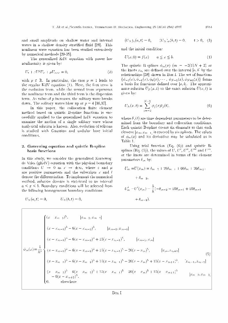
Abstract. The collocation �nite element method was applied to obtain solitary wavesolutions to Korteweg-de Vries equation with power law nonlinearity. The stability anderror analyses were also carried out for these waves. Additionally, conservation laws werestudied numerically.

© 2018 Sharif University of Technology. All rights reserved.

1. Introduction

The dynamics of shallow water waves has been anactive research area during the past several decades. Inthis context, there are several models that govern thiswave ow. A few of these commonly studied modelsare Boussinesq equation [1], Kawahara equation [2],Peregrine equation [3], Benjamin-Bona-Mahoney equa-tion [4], and several others [5-8]. This paper studiesthe model with the aid of Korteweg-de Vries (KdV)equation. In order to keep this on a generalized setting,power law nonlinearity is considered; note that theKdV equation and modi�ed KdV equation becomespecial cases.

There are several analytical and numericalschemes that are applied to understand the shal-

*. Corresponding author.E-mail address: [email protected] (T. Ak)

doi: 10.24200/sci.2017.4518

low water wave phenomena [9-13]. Some ofthese algorithms are exp-function method, G0=G-expansion scheme [14,15], method of undeterminedcoe�cients, semi-inverse variational principle, Galerkinmethod [16,17], Petrov-Galerkin method [18], colloca-tion method [19-21], and several others [22-24]. Also,the solutions to some fractional di�erential equationshave been discussed [25,26]. This paper studies powerlaw KdV equation by using collocation �nite elementmethod. The stability analysis as well as conservationlaws are both addressed.

The well-known Korteweg-de Vries (KdV) equa-tion:

Ut + "UUx + �Uxxx = 0; (1)

where " and � are the nonlinear and dispersion co-e�cients, respectively, is the generic model for thestudy of weakly nonlinear long waves [27]. It arisesin physical systems, which involve a balance betweennonlinearity and dispersion at leading-order [28]. Forexample, it describes surface waves of long wavelength

T. Ak et al./Scientia Iranica, Transactions B: Mechanical Engineering 25 (2018) 2582{2597 2583

and small amplitude on shallow water and internalwaves in a shallow density-strati�ed uid [28]. Thisnonlinear wave equation has been studied extensivelyby numerical methods [29-35].

The generalized KdV equation with power lawnonlinearity is given by:

Ut + "UpUx + �Uxxx = 0; (2)

with p 2 R. In particular, the case p = 1 leads tothe regular KdV equation (1). Here, the �rst term isthe evolution term, while the second term representsthe nonlinear term and the third term is the dispersionterm. As value of p increases, the solitary wave breaksdown. The solitary waves blow up at p = 4 [36,37].

In this paper, the collocation �nite elementmethod based on quintic B-spline functions is suc-cessfully applied to the generalized KdV equation toexamine the motion of a single solitary wave whoseanalytical solution is known. Also, evolution of solitonsis studied with Gaussian and undular bore initialconditions.

2. Governing equation and quintic B-splinebasis functions

In this study, we consider the generalized Korteweg-de Vries (gKdV) equation with the physical boundaryconditions U ! 0 as x ! �1, where " and �are positive parameters and the subscripts x and tdenote the di�erentiation. To implement the numericalmethod, solution domain is restricted to an intervala � x � b: Boundary conditions will be selected fromthe following homogeneous boundary conditions:

UN (a; t) = 0; UN (b; t) = 0;

(UN )x(a; t) = 0; (UN )x(b; t) = 0; t > 0; (3)

and the initial condition:

U(x; 0) = f(x) a � x � b: (4)

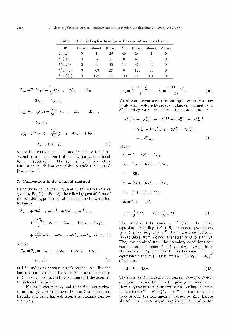
The quintic B-splines �m(x) (m = �2(1)N + 2) atthe knots xm are de�ned over the interval [a; b] by therelationships [38] shown in Box I. The set of functionsf��2(x); ��1(x); �0(x); � � � ; �N+1(x); �N+2(x)g formsa basis for functions de�ned over [a; b]. The approxi-mate solution UN (x; t) to the exact solution U(x; t) isgiven by:

UN (x; t) =N+2Xj=�2

�j(x)�j(t); (6)

where �j(t) are time dependent parameters to be deter-mined from the boundary and collocation conditions.Each quintic B-spline covers six elements so that eachelement [xm; xm+1] is covered by six splines. The valuesof �m(x) and its derivative may be tabulated as inTable 1.

Using trial function (Eq. (6)) and quintic B-splines (Eq. (5)), the values of U , U 0, U 00, U 000 and U iv,at the knots are determined in terms of the elementparameters �m by:

Um =U(xm) = �m�2 + 26�m�1 + 66�m + 26�m+1

+ �m+2;

U 0m =U 0(xm) =5h

(��m�2 � 10�m�1 + 10�m+1

+ �m+2);

�m(x)=1h5

8>>>>>>>>>>>>>>>>>>>>>>>><>>>>>>>>>>>>>>>>>>>>>>>>:

(x� xm�3)5; [xm�3; xm�2]

(x� xm�3)5 � 6(x� xm�2)5; [xm�2; xm�1]

(x� xm�3)5 � 6(x� xm�2)5 + 15(x� xm�1)5; [xm�1; xm]

(x� xm�3)5 � 6(x� xm�2)5 + 15(x� xm�1)5 � 20(x� xm)5; [xm; xm+1]

(x� xm�3)5 � 6(x� xm�2)5 + 15(x� xm�1)5 � 20(x� xm)5 + 15(x� xm+1)5; [xm+1; xm+2]

(x� xm�3)5 � 6(x� xm�2)5 + 15(x� xm�1)5 � 20(x� xm)5 + 15(x� xm+1)5

� 6(x� xm+2)5; [xm+2; xm+3]

0: elsewhere

(5)

Box I

2584 T. Ak et al./Scientia Iranica, Transactions B: Mechanical Engineering 25 (2018) 2582{2597

Table 1. Quintic B-spline function and its derivatives at nodes xm.

x xm�3 xm�2 xm�1 xm xm+1 xm+2 xm+3

�m(x) 0 1 26 66 26 1 0h�0m(x) 0 -5 -50 0 50 5 0h2�00m(x) 0 20 40 -120 40 20 0h3�000m(x) 0 -60 120 0 -120 60 0h4�ivm(x) 0 120 -480 720 -480 120 0

U 00m =U 00(xm) =20h2 (�m�2 + 2�m�1 � 6�m

+ 2�m+1 + �m+2);

U 000m =U 000(xm) =60h3 (��m�2 + 2�m�1 � 2�m+1

+ �m+2);

U ivm =U iv(xm) =120h4 (�m�2 � 4�m�1 + 6�m

� 4�m+1 + �m+2); (7)

where the symbols 0, 00, 000, and iv denote the �rst,second, third, and fourth di�erentiation with respectto x, respectively. The splines �m(x) and theirfour principal derivatives vanish outside the interval[xm�3; xm+3].

3. Collocation �nite element method

Using the nodal values of Um and its spatial derivativesgiven by Eq. (7) in Eq. (2), the following general form ofthe solution approach is obtained for the linearizationtechnique:

_�m�2 + 26 _�m�1 + 66 _�m + 26 _�m+1 + _�m+2

+5"Zmh

(��m�2�10�m�1+10�m+1+�m+2)

+60�h3 (��m�2+2�m�1�2�m+1+�m+2)=0; (8)

where:

Zm =Upm = (�m�2 + 26�m�1 + 66�m + 26�m+1

+ �m+2)p; (9)

and \." indicates derivative with respect to t. For thelinearization technique, the term Up in non-linear termUpUx is taken as Eq. (9) by assuming that the quantityUp is locally constant.

If time parameters �i and their time derivatives_�i in Eq. (8) are discretized by the Crank-Nicolsonformula and usual �nite di�erence approximation, re-spectively:

�i =�n+1i + �ni

2; _�i =

�n+1i � �ni

�t: (10)

We obtain a recurrence relationship between two timelevels n and n+ 1 relating two unknown parameters in�n+1i and �ni for i = m� 2;m� 1; � � � ;m+ 1;m+ 2:

1�n+1m�2 + 2�n+1

m�1 + 3�n+1m + 4�n+1

m+1 + 5�n+1m+2

= 5�nm�2 + 4�nm�1 + 3�nm + 2�nm+1

+ 1�nm+2; (11)

where:

1 = [1� EZm �M ];

2 = [26� 10EZm + 2M ];

3 = [66];

4 = [26 + 10EZm � 2M ];

5 = [1 + EZm +M ];

m = 0; 1; � � � ; N;

E =5

2h"�t; M =

30h3��t: (12)

The system (11) consists of (N + 1) linearequations including (N + 5) unknown parameters(��2; ��1; � � � ; �N+1; �N+2)T . To obtain a unique solu-tion to this system, we need four additional constraints.They are obtained from the boundary conditions andcan be used to eliminate ��2, ��1 and �N+1, �N+2 fromthe system in Eq. (11), which later becomes a matrixequation for the N + 1 unknowns d = (�0; �1; � � � ; �N )Tof the form:

Adn+1 = Bdn: (13)

The matrices A and B are pentagonal (N+1)�(N+1)and can be solved by using the pentagonal algorithm.However, two or three inner iterations are implementedfor the term �n� = �n + 1

2 (�n� �n�1) at each time stepto cope with the non-linearity caused by Zm. Beforethe solution process begins iteratively, the initial vector


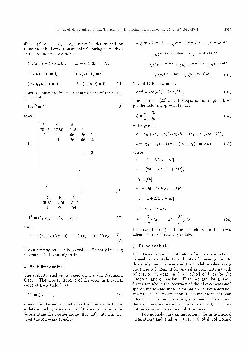
d0 = (�0; �1; � � � ; �N�1; �N ) must be determined byusing the initial condition and the following derivativesat the boundary conditions:

UN (x; 0) = U(xm; 0); m = 0; 1; 2; � � � ; N;(UN )x(a; 0) = 0; (UN )x(b; 0) = 0;

(UN )xx(a; 0) = 0; (UN )xx(b; 0) = 0: (14)

Thus, we have the following matrix form of the initialvector d0:

Wd0 = C; (15)

where:

W =

2666666666664

54 60 625:25 67:50 26:25 1

1 26 66 26 11 26 66 26

. . .1 26

1

1

66 26 126:25 67:50 25:25

6 60 54

377777777775; (16)

d0 = (�0; �1; � � � ; �N�1; �N ); (17)

and:

C=[U(x0; 0); U(x1; 0); � � � ; U(xN�1; 0); U(xN ; 0)]T :(18)

This matrix system can be solved be e�ciently by usinga variant of Thomas algorithm.

4. Stability analysis

The stability analysis is based on the Von Neumanntheory. The growth factor � of the error in a typicalmode of amplitude �n is:

�nm = �neimkh; (19)

where k is the mode number and h, the element size,is determined by linearization of the numerical scheme.Substituting the Fourier mode (Eq. (19)) into Eq. (11)gives the following equality:

1�n+1ei(m�2)kh + 2�n+1ei(m�1)kh + 3�n+1eimkh

+ 4�n+1ei(m+1)kh + 5�n+1ei(m+2)kh

= 5�nei(m�2)kh + 4�nei(m�1)kh + 3�neimkh

+ 2�nei(m+1)kh + 1�nei(m+2)kh: (20)

Now, if Euler's formula:

eikh = cos(kh) + i sin(kh); (21)

is used in Eq. (20) and this equation is simpli�ed, weget the following growth factor:

� =a� iba+ ib

; (22)

which gives:

a = 3 + ( 2 + 4) cos(kh) + ( 1 + 5) cos(2kh);

b = ( 4 � 2) sin(kh) + ( 5 � 1) sin(2kh); (23)

where:

1 = [1� EZm �M ];

2 = [26� 10EZm + 2M ];

3 = [66];

4 = [26 + 10EZm � 2M ];

5 = [1 + EZm +M ];

m = 0; 1; � � � ; N;

E =5

2h"�t; M =

30h3��t: (24)

The modulus of � is 1 and therefore, the linearizedscheme is unconditionally stable.

5. Error analysis

The e�ciency and acceptability of a numerical schemedepend on its stability and rate of convergence. Inthis study, we approximated the model problem usingpiecewise polynomials for spatial approximations withcollocation approach and a method of lines for thetemporal approximation. Here, we aim for a shortdiscussion about the accuracy of the above-mentionedspace time scheme without formal proof. For a detailedanalysis and discussion about this issue, the readers canrefer to Bochev and Gunzburger [39] and the referencestherein. Here, we use some constants Ci � 0, which arenot necessarily the same in all the cases.

Polynomials play an important role in numericalintegrations and analysis [37,40]. Global polynomial


interpolations can be used to integrate the solutionsto di�erential equations when the unknown curves areconsidered to be very smooth. However, there aremany practical situations in engineering and physicalproblems that the solutions are not su�ciently smoothto support global polynomial approximation. In thesecases, piecewise polynomial interpolations play animportant role and work very well to integrate thesolutions. One of the main bene�ts of using polynomialbasis functions is that they have smooth curves. Ingeneral, if we have k + 1 data points, then there isexactly one polynomial of degree at most k passingthrough the data points and the error in the interpo-lating polynomial is proportional to the power of thedistance between the data points. A detailed discussionabout the polynomial approximation and least squarespiecewise polynomials approximations can be foundin [37,39,40]. Moreover, the main bene�t of usingcollocation scheme is that it gives super-convergencepointwise approximation. Compared with the Galerkininner product approach, the collocation approach doesnot require an extra integral for evaluation. Thus,this approach is simpler and more e�cient to computesolutions.

Let Hr() be the space of r times di�erentiablefunctions and k:kr be the standard Hr() norm. Letvh be an approximation to a function v(x) 2 Hr()in . Let h be the distance between the grids and = [ii, where i = [xi; xi+1], xi+1 = xi + h. Weobserve [37,40,41] that:

kv(x)�vh(x)k�C�xk+1kvkk+1; 1 � k < r; (25)

and vh stands for interpolation by piecewise polynomi-als of degree r (considering = [ii). This error ispreserved by the Galerkin �nite element approximationas well [40].

It can be easily observed [39,40] that if wh is asuitable B-spline de�ned by a polynomial of degree lessthan or equal to k, then:

kw(x)�wh(x)k�C�xl+1kwkl+1; 1 � l < k; (26)

for any w 2 Hk(). In this study, we use quintic B-splines for space integration. Thus, from the abovediscussion, one sees that we obtain anO(�x6) accuracyfor the spatial approximation in L2() norm, becausefor time, we use the Crank-Nicolson scheme, which isof O(�t2) accuracy in L2([0; T ]) norm for some T > 0,followed by a forward di�erence scheme, which is ofO(�t) accuracy in L2([0; T ]) norm for some T > 0 [40].Therefore, we obtain the error bound as:

ku(x; t)� uh(x; t)k � C1�x6 + C2�t2 + C3�t

= C1�x6 + C2�t; (27)

for suitable C1 � 0 and C2 � 0.In addition, the convergence order of Crank-

Nicolson method for the temporal variable is quadratic.The development of stability and higher order conver-gence scheme according to time variable is subject ofthe further investigations.

6. Numerical simulations

Numerical results of the gKdV equation are obtainedfor two problems: the motion of single solitary wave,evolution of solitons with Gaussian and undular boreinitial conditions. We use the error norm L2 that isde�ned as:

L2 = U exact�UN 2 '

vuuthNXj=1

��U exactj �(UN )j

��2;(28)

and the error norm L1:

L1 = U exact � UN 1 ' max

j

��U exactj � (UN )j

�� ;j = 1; 2; � � � ; N; (29)

to calculate the di�erence between analytical andnumerical solutions at some speci�ed times. Thegeneralized KdV equation (Eq. (2)) possesses onlythree invariants by:

I1 =Z b

aUdx ' h

NXj=1

Unj ;

I2 =Z b

aU2dx ' h

NXj=1

(Unj )2;

I3 =Z b

a

�Up+2 � �(p+ 1)(p+ 2)

2"(Ux)2

�dx

' hNXj=1

�(Unj )p+2 � �(p+ 1)(p+ 2)

2"(Ux)2

j

�; (30)

which correspond to conversation laws. In the simu-lation of solitary wave motion, the invariants I1, I2,and I3 are monitored to check the conversation of thenumerical algorithm.

6.1. The motion of single solitary waveThe single solitary wave solution of the gKdV equation(Eq. (2)) considered by the boundary conditions U ! 0as x! �1 is given by:

U(x; t) = Asech2p [k(x� ct)]; (31)

where A = [ c(p+1)(p+2)2" ]

1p and k = p

2

qc� [36]. Note

that, c, ", �, and p are arbitrary constants. The initialcondition is:


U(x; 0) = Asech2p (kx): (32)

To show the motion of the single solitary wave solutionnumerically, let " = 1, � = 4:84 � 10�4, c = 0:3, andx� [0; 2]. Now, we consider the following cases.

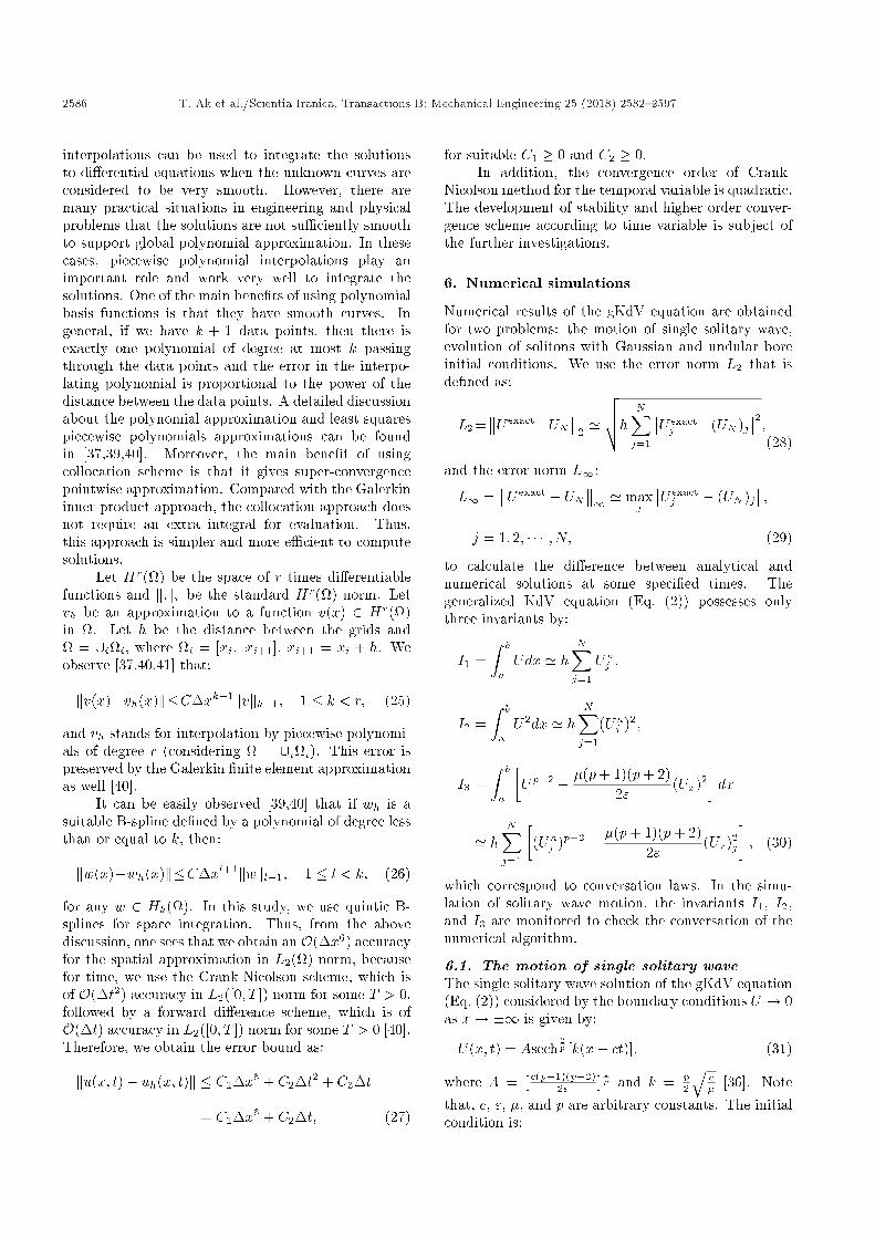
6.1.1. Case IFor p = 1, parameters are chosen as " = 1, � = 4:84�10�4, c = 0:3, h = 0:01, and �t = 0:005 to correspondwith those in the earlier studies. For these parameters,the single solitary wave has the amplitude = 0:9. Theconserved quantities and error norms, L2 and L1, areshown at selected times up to time t = 3. The obtainedresults are tabulated in Table 2. It can be seen fromTable 2 that the error norms L2 and L1 are smallenough and the invariants are nearly unchanged duringthe process time. It is observed in the tables thatpercentages of relative changes of I1, I2, and I3 are6:33�10�4, 3:41�10�7, and 7:53� 10�7, respectively.Table 2 represents a comparison of the values of theinvariants and error norms obtained by the presentmethod with earlier results. Numerical solution ofsingle solitary wave is plotted at selected times fromt = 0 to t = 3 in Figure 1.

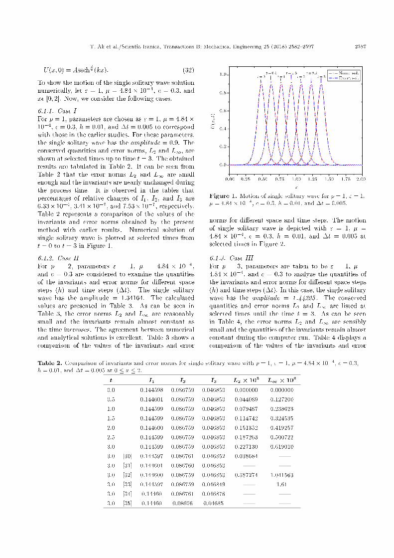
6.1.2. Case IIFor p = 2, parameters " = 1, � = 4:84 � 10�4,and c = 0:3 are considered to examine the quantitiesof the invariants and error norms for di�erent spacesteps (h) and time steps (�t). The single solitarywave has the amplitude = 1:34164. The calculatedvalues are presented in Table 3. As can be seen inTable 3, the error norms L2 and L1 are reasonablysmall and the invariants remain almost constant asthe time increases. The agreement between numericaland analytical solutions is excellent. Table 3 shows acomparison of the values of the invariants and error

Figure 1. Motion of single solitary wave for p = 1, " = 1,� = 4:84� 10�4; c = 0:3, h = 0:01, and �t = 0:005.

norms for di�erent space and time steps. The motionof single solitary wave is depicted with " = 1, � =4:84 � 10�4, c = 0:3, h = 0:01, and �t = 0:005 atselected times in Figure 2.

6.1.3. Case IIIFor p = 3, parameters are taken to be " = 1, � =4:84 � 10�4, and c = 0:3 to analyze the quantities ofthe invariants and error norms for di�erent space steps(h) and time steps (�t). In this case, the single solitarywave has the amplitude = 1 :44225 . The conservedquantities and error norms L2 and L1 are listed atselected times until the time t = 3. As can be seenin Table 4, the error norms L2 and L1 are sensiblysmall and the quantities of the invariants remain almostconstant during the computer run. Table 4 displays acomparison of the values of the invariants and error

Table 2. Comparison of invariants and error norms for single solitary wave with p = 1, " = 1, � = 4:84� 10�4, c = 0:3,h = 0:01, and �t = 0:005 at 0 � x � 2.

t I1 I2 I3 L2 � 103 L1 � 103

0.0 0.144598 0.086759 0.046850 0.000000 0.0000000.5 0.144601 0.086759 0.046850 0.044089 0.1272001.0 0.144599 0.086759 0.046850 0.079487 0.2386231.5 0.144599 0.086759 0.046850 0.114742 0.3245352.0 0.144600 0.086759 0.046850 0.151352 0.4192572.5 0.144599 0.086759 0.046850 0.187263 0.5007223.0 0.144599 0.086759 0.046850 0.227130 0.6190103.0 [30] 0.144597 0.086761 0.046852 0.038684 |3.0 [31] 0.144601 0.086760 0.046850 | |3.0 [32] 0.144600 0.086759 0.046850 0.387274 1.0415633.0 [33] 0.144597 0.086759 0.046849 | 1.613.0 [34] 0.14460 0.086761 0.046876 | |3.0 [35] 0.14460 0.08676 0.04685 | |


Table 3. Comparison of invariants and error norms for single solitary wave with p = 2, " = 1, � = 4:84� 10�4, andc = 0:3 at 0 � x � 2.

t L2 � 103 L1 � 103 I1 I2 I3

h = 0:01�t = 0:005

0.0 0.000000 0.000000 0.169296 0.144599 0.0867600.5 0.161944 0.574891 0.169300 0.144599 0.0867601.0 0.318711 1.054684 0.169292 0.144599 0.0867601.5 0.460453 1.582264 0.169294 0.144599 0.0867602.0 0.607800 1.948279 0.169295 0.144599 0.0867602.5 0.752947 2.376394 0.169297 0.144599 0.0867603.0 0.912455 2.886583 0.169297 0.144599 0.086760

h = 0:005�t = 0:0025

0.0 0.000000 0.000000 0.169296 0.144599 0.0867590.5 0.063939 0.208079 0.169298 0.144599 0.0867591.0 0.125994 0.397920 0.169297 0.144599 0.0867591.5 0.188595 0.585358 0.169297 0.144599 0.0867592.0 0.250310 0.769922 0.169297 0.144599 0.0867592.5 0.313310 0.977050 0.169297 0.144599 0.0867593.0 0.375889 1.158590 0.169297 0.144599 0.086759

h = 0:001�t = 0:0005

0.0 0.000000 0.000000 0.169298 0.144601 0.0867630.5 0.012709 0.034070 0.169300 0.144601 0.0867631.0 0.020823 0.056822 0.169299 0.144601 0.0867631.5 0.023853 0.069660 0.169299 0.144601 0.0867632.0 0.058242 0.209984 0.169299 0.144601 0.0867632.5 0.113519 0.380739 0.169299 0.144601 0.0867633.0 0.168194 0.543238 0.169300 0.144601 0.086763

Figure 2. Motion of single solitary wave for p = 2, " = 1,� = 4:84� 10�4, c = 0:3, h = 0:01, and �t = 0:005.

norms for di�erent space and time steps. In Figure 3,the propagation of single solitary wave is illustratedwith " = 1, � = 4:84 � 10�4, c = 0:3, h = 0:01,and �t = 0:005 at selected times from t = 0 tot = 3.

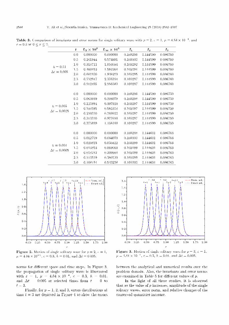
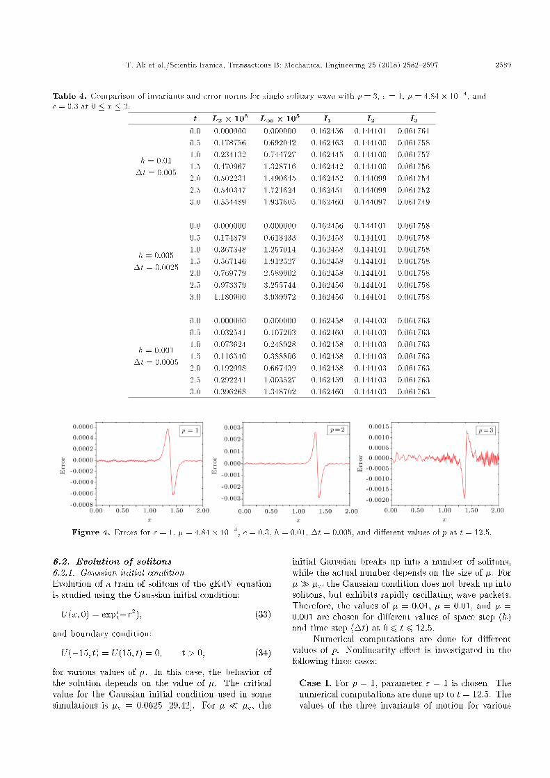
Finally, for p = 1, 2, and 3, errors distributions attime t = 3 are depicted in Figure 4 to show the errors

Figure 3. Motion of single solitary wave for p = 3, " = 1,� = 4:84� 10�4, c = 0:3, h = 0:01, and �t = 0:005.

between the analytical and numerical results over theproblem domain. Also, the invariants and error normsare examined in Table 5 for di�erent values of p.

In the light of all these studies, it is observedthat as the value of p increases, amplitude of the singlesolitary waves, error norm, and relative changes of theconserved quantities increase.


Table 4. Comparison of invariants and error norms for single solitary wave with p = 3, " = 1, � = 4:84� 10�4, andc = 0:3 at 0 � x � 2.

t L2 � 103 L1 � 103 I1 I2 I3

h = 0:01�t = 0:005

0.0 0.000000 0.000000 0.162456 0.144101 0.0617610.5 0.178756 0.692042 0.162463 0.144100 0.0617581.0 0.234132 0.744727 0.162445 0.144100 0.0617571.5 0.470967 1.328716 0.162442 0.144100 0.0617562.0 0.502231 1.490645 0.162452 0.144099 0.0617542.5 0.540347 1.721624 0.162451 0.144099 0.0617523.0 0.554489 1.937605 0.162460 0.144097 0.061749

h = 0:005�t = 0:0025

0.0 0.000000 0.000000 0.162456 0.144101 0.0617580.5 0.174879 0.613433 0.162458 0.144101 0.0617581.0 0.367348 1.257014 0.162458 0.144101 0.0617581.5 0.567146 1.912527 0.162458 0.144101 0.0617582.0 0.769779 2.589902 0.162458 0.144101 0.0617582.5 0.973379 3.255744 0.162456 0.144101 0.0617583.0 1.180900 3.939972 0.162456 0.144101 0.061758

h = 0:001�t = 0:0005

0.0 0.000000 0.000000 0.162458 0.144103 0.0617630.5 0.032541 0.107203 0.162460 0.144103 0.0617631.0 0.073624 0.248928 0.162458 0.144103 0.0617631.5 0.116540 0.388806 0.162458 0.144103 0.0617632.0 0.192098 0.667439 0.162458 0.144103 0.0617632.5 0.292241 1.003527 0.162459 0.144103 0.0617633.0 0.396268 1.348702 0.162460 0.144103 0.061763

Figure 4. Errors for " = 1, � = 4:84� 10�4, c = 0:3, h = 0:01, �t = 0:005, and di�erent values of p at t = 12:5.

6.2. Evolution of solitons6.2.1. Gaussian initial conditionEvolution of a train of solitons of the gKdV equationis studied using the Gaussian initial condition:

U(x; 0) = exp(�x2); (33)

and boundary condition:

U(�15; t) = U(15; t) = 0; t > 0; (34)

for various values of �. In this case, the behavior ofthe solution depends on the value of �. The criticalvalue for the Gaussian initial condition used in somesimulations is �c = 0:0625 [29,42]. For � � �c, the

initial Gaussian breaks up into a number of solitons,while the actual number depends on the size of �. For�� c, the Gaussian condition does not break up intosolitons, but exhibits rapidly oscillating wave packets.Therefore, the values of � = 0:04, � = 0:01, and � =0:001 are chosen for di�erent values of space step (h)and time step (�t) at 0 6 t 6 12:5.

Numerical computations are done for di�erentvalues of p. Nonlinearity e�ect is investigated in thefollowing three cases:

Case I. For p = 1, parameter " = 1 is chosen. Thenumerical computations are done up to t = 12:5. Thevalues of the three invariants of motion for various


Table 5. Invariants and error norms for single solitary wave with " = 1, � = 4:84� 10�4, c = 0:3, h = 0:01, and�t = 0:005.

t L2 � 103 L1 � 103 I1 I2 I3

p = 1

0.0 0.000000 0.000000 0.144598 0.086759 0.0468500.5 0.044089 0.127200 0.144601 0.086759 0.0468501.0 0.079487 0.238623 0.144599 0.086759 0.0468501.5 0.114742 0.324535 0.144599 0.086759 0.0468502.0 0.151352 0.419257 0.144600 0.086759 0.0468502.5 0.187263 0.500722 0.144599 0.086759 0.0468503.0 0.227130 0.619010 0.144599 0.086759 0.046850

p = 2

0.0 0.000000 0.000000 0.169296 0.144599 0.0867600.5 0.161944 0.574891 0.169300 0.144599 0.0867601.0 0.318711 1.054684 0.169292 0.144599 0.0867601.5 0.460453 1.582264 0.169294 0.144599 0.0867602.0 0.607800 1.948279 0.169295 0.144599 0.0867602.5 0.752947 2.376394 0.169297 0.144599 0.0867603.0 0.912455 2.886583 0.169297 0.144599 0.086760

p = 3

0.0 0.000000 0.000000 0.162456 0.144101 0.0617610.5 0.178756 0.692042 0.162463 0.144100 0.0617581.0 0.234132 0.744727 0.162445 0.144100 0.0617571.5 0.470967 1.328716 0.162442 0.144100 0.0617562.0 0.502231 1.490645 0.162452 0.144099 0.0617542.5 0.540347 1.721624 0.162451 0.144099 0.0617523.0 0.554489 1.937605 0.162460 0.144097 0.061749

Table 6. Invariants for Gaussian initial condition with p = 1, " = 1, and c = 0:3 at �15 � x � 15.

p = 1 � = 0:04 � = 0:01 � = 0:001t I1 I2 I3 I1 I2 I3 I1 I2 I3

0.0 1.772454 1.253314 0.872929 1.772454 1.253314 0.985727 1.772454 1.253314 1.0195672.5 1.772484 1.253314 0.872921 1.772458 1.253324 0.985589 1.772452 1.253317 1.0195615.0 1.772454 1.253315 0.872919 1.772419 1.253344 0.985538 1.772454 1.253319 1.0195477.5 1.774643 1.253828 0.872915 1.772553 1.253363 0.985557 1.772458 1.253320 1.01954710.0 1.774464 1.253579 0.872979 1.772360 1.253381 0.985579 1.772447 1.253321 1.01954812.5 1.763884 1.257298 0.872872 1.772730 1.253429 0.985626 1.772452 1.253321 1.019549

h = 0:1 �t = 0:01 h = 0:1 �t = 0:01 h = 0:01 �t = 0:005

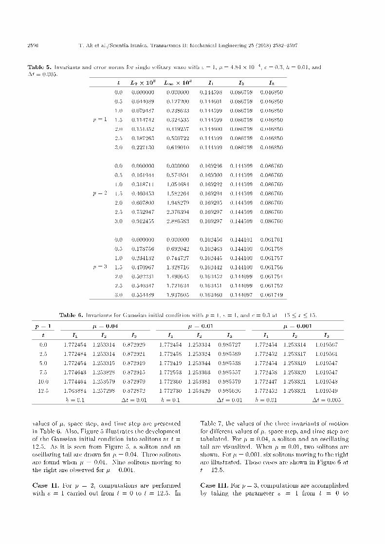
values of �, space step, and time step are presentedin Table 6. Also, Figure 5 illustrates the developmentof the Gaussian initial condition into solitons at t =12:5. As it is seen from Figure 5, a soliton and anoscillating tail are drawn for � = 0:04. Three solitonsare found when � = 0:01. Nine solitons moving tothe right are observed for � = 0:001.

Case II. For p = 2, computations are performedwith " = 1 carried out from t = 0 to t = 12:5. In

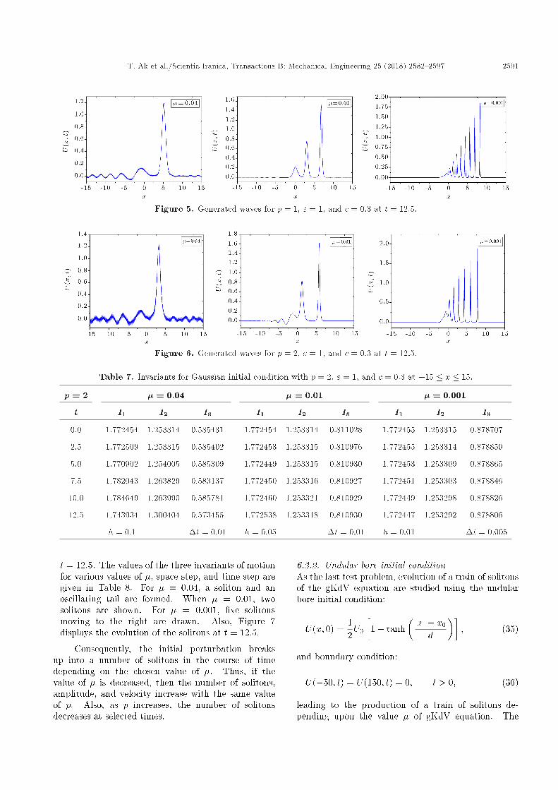
Table 7, the values of the three invariants of motionfor di�erent values of �, space step, and time step aretabulated. For � = 0:04, a soliton and an oscillatingtail are visualized. When � = 0:01, two solitons areshown. For � = 0:001, six solitons moving to the rightare illustrated. These cases are shown in Figure 6 att = 12:5.

Case III. For p = 3, computations are accomplishedby taking the parameter " = 1 from t = 0 to


Figure 5. Generated waves for p = 1, " = 1, and c = 0:3 at t = 12:5.



p = 2 � = 0:04 � = 0:01 � = 0:001

t I1 I2 I3 I1 I2 I3 I1 I2 I3

0.0 1.772454 1.253314 0.585431 1.772454 1.253314 0.811028 1.772455 1.253315 0.878707

2.5 1.772509 1.253315 0.585402 1.772453 1.253315 0.810976 1.772455 1.253314 0.878859

5.0 1.770902 1.254005 0.585309 1.772449 1.253315 0.810930 1.772453 1.253309 0.878865

7.5 1.782043 1.263829 0.583137 1.772450 1.253316 0.810927 1.772451 1.253303 0.878846

10.0 1.784649 1.263990 0.585781 1.772460 1.253321 0.810929 1.772449 1.253298 0.878826

12.5 1.743934 1.300404 0.573455 1.772538 1.253318 0.810930 1.772447 1.253292 0.878806

h = 0:1 �t = 0:01 h = 0:05 �t = 0:01 h = 0:01 �t = 0:005

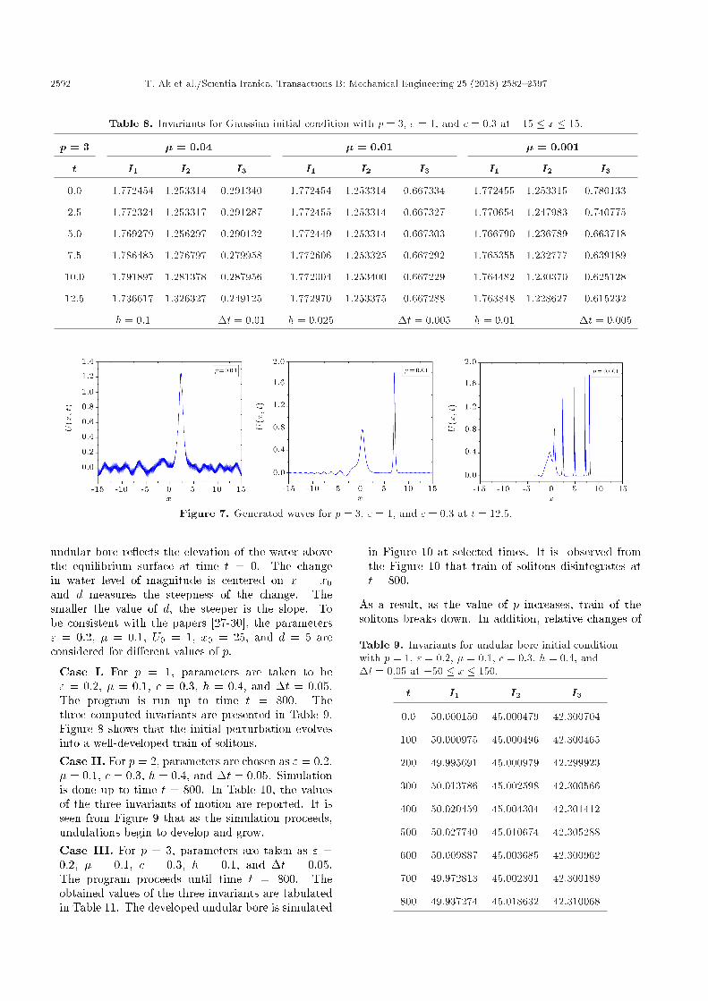
t = 12:5. The values of the three invariants of motionfor various values of �, space step, and time step aregiven in Table 8. For � = 0:04, a soliton and anoscillating tail are formed. When � = 0:01, twosolitons are shown. For � = 0:001, �ve solitonsmoving to the right are drawn. Also, Figure 7displays the evolution of the solitons at t = 12:5.

Consequently, the initial perturbation breaksup into a number of solitons in the course of timedepending on the chosen value of �. Thus, if thevalue of � is decreased, then the number of solitons,amplitude, and velocity increase with the same valueof p. Also, as p increases, the number of solitonsdecreases at selected times.

6.2.2. Undular bore initial conditionAs the last test problem, evolution of a train of solitonsof the gKdV equation are studied using the undularbore initial condition:

U(x; 0) =12U0

�1� tanh

� jxj � x0

d

��; (35)

and boundary condition:

U(�50; t) = U(150; t) = 0; t > 0; (36)

leading to the production of a train of solitons de-pending upon the value � of gKdV equation. The



p = 3 � = 0:04 � = 0:01 � = 0:001

t I1 I2 I3 I1 I2 I3 I1 I2 I3

0.0 1.772454 1.253314 0.291340 1.772454 1.253314 0.667334 1.772455 1.253315 0.780133

2.5 1.772324 1.253317 0.291287 1.772455 1.253314 0.667327 1.770654 1.247983 0.740775

5.0 1.769279 1.256297 0.290132 1.772449 1.253314 0.667303 1.766790 1.236789 0.663718

7.5 1.786485 1.276797 0.279958 1.772606 1.253325 0.667292 1.765355 1.232777 0.639189

10.0 1.791897 1.281378 0.287956 1.772004 1.253400 0.667229 1.764482 1.230370 0.625128

12.5 1.736617 1.326327 0.249125 1.772970 1.253375 0.667288 1.763848 1.228627 0.615232

h = 0:1 �t = 0:01 h = 0:025 �t = 0:005 h = 0:01 �t = 0:005


undular bore re ects the elevation of the water abovethe equilibrium surface at time t = 0. The changein water level of magnitude is centered on x = x0and d measures the steepness of the change. Thesmaller the value of d, the steeper is the slope. Tobe consistent with the papers [27-30], the parameters" = 0:2, � = 0:1, U0 = 1, x0 = 25, and d = 5 areconsidered for di�erent values of p.

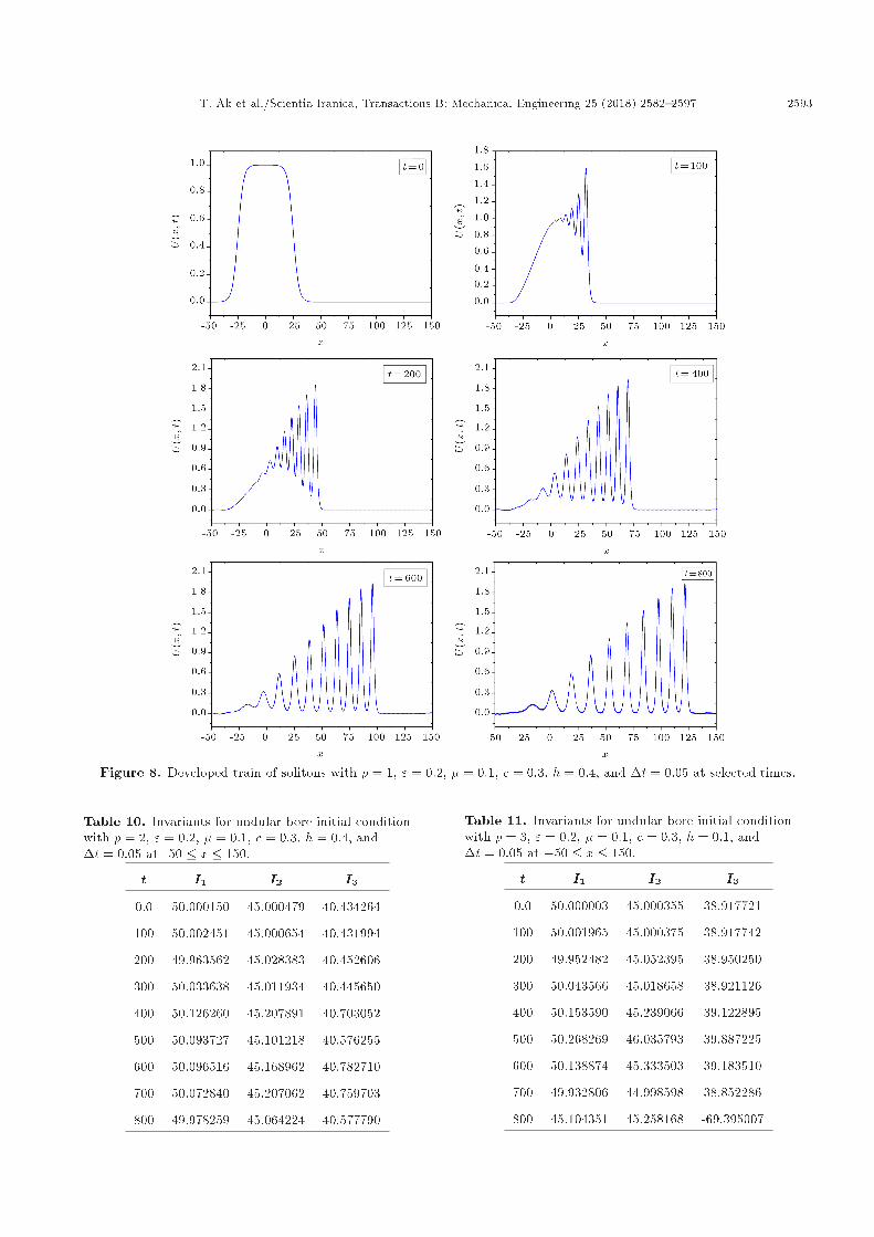
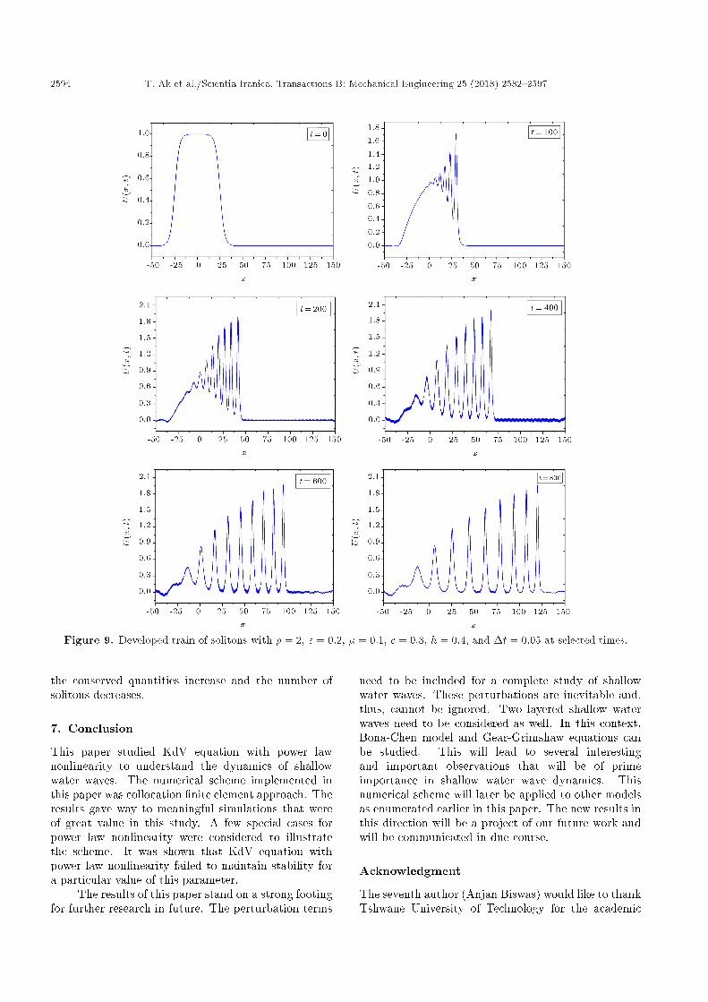
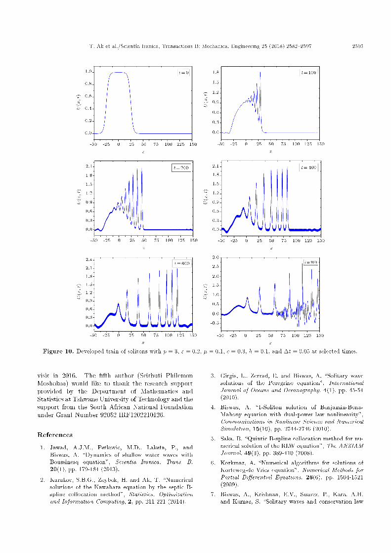
Case I. For p = 1, parameters are taken to be" = 0:2, � = 0:1, c = 0:3, h = 0:4, and �t = 0:05.The program is run up to time t = 800. Thethree computed invariants are presented in Table 9.Figure 8 shows that the initial perturbation evolvesinto a well-developed train of solitons.Case II. For p = 2, parameters are chosen as " = 0:2,� = 0:1, c = 0:3, h = 0:4, and �t = 0:05. Simulationis done up to time t = 800. In Table 10, the valuesof the three invariants of motion are reported. It isseen from Figure 9 that as the simulation proceeds,undulations begin to develop and grow.Case III. For p = 3, parameters are taken as " =0:2, � = 0:1, c = 0:3, h = 0:1, and �t = 0:05.The program proceeds until time t = 800. Theobtained values of the three invariants are tabulatedin Table 11. The developed undular bore is simulated

in Figure 10 at selected times. It is observed fromthe Figure 10 that train of solitons disintegrates att = 800.

As a result, as the value of p increases, train of thesolitons breaks down. In addition, relative changes of

Table 9. Invariants for undular bore initial conditionwith p = 1, " = 0:2, � = 0:1, c = 0:3, h = 0:4, and�t = 0:05 at �50 � x � 150.

t I1 I2 I3

0.0 50.000150 45.000479 42.300704

100 50.000975 45.000496 42.300465

200 49.995691 45.000979 42.299923

300 50.013786 45.002598 42.300566

400 50.020459 45.004304 42.301412

500 50.027740 45.010674 42.305288

600 50.009887 45.003685 42.300962

700 49.972813 45.002301 42.300189

800 49.937274 45.018632 42.310068


Figure 8. Developed train of solitons with p = 1, " = 0:2, � = 0:1, c = 0:3, h = 0:4, and �t = 0:05 at selected times.

Table 10. Invariants for undular bore initial conditionwith p = 2, " = 0:2, � = 0:1, c = 0:3, h = 0:4, and�t = 0:05 at�50 � x � 150.

t I1 I2 I3

0.0 50.000150 45.000479 40.434264

100 50.002451 45.000654 40.431994

200 49.963562 45.028383 40.452606

300 50.033638 45.011934 40.445650

400 50.126260 45.207891 40.703052

500 50.093727 45.101218 40.576255

600 50.096516 45.168962 40.782710

700 50.072840 45.207062 40.759703

800 49.978259 45.064224 40.577790

Table 11. Invariants for undular bore initial conditionwith p = 3, " = 0:2, � = 0:1, c = 0:3, h = 0:1, and�t = 0:05 at �50 � x � 150.

t I1 I2 I3

0.0 50.000003 45.000355 38.917721

100 50.001965 45.000375 38.917742

200 49.952482 45.052395 38.950250

300 50.043566 45.018658 38.921126

400 50.153590 45.239066 39.122895

500 50.268269 46.035793 39.887225

600 50.138874 45.333503 39.183510

700 49.932806 44.998598 38.852286

800 45.104351 45.258168 -69.395007



the conserved quantities increase and the number ofsolitons decreases.

7. Conclusion

This paper studied KdV equation with power lawnonlinearity to understand the dynamics of shallowwater waves. The numerical scheme implemented inthis paper was collocation �nite element approach. Theresults gave way to meaningful simulations that wereof great value in this study. A few special cases forpower law nonlinearity were considered to illustratethe scheme. It was shown that KdV equation withpower law nonlinearity failed to maintain stability fora particular value of this parameter.

The results of this paper stand on a strong footingfor further research in future. The perturbation terms

need to be included for a complete study of shallowwater waves. These perturbations are inevitable and,thus, cannot be ignored. Two layered shallow waterwaves need to be considered as well. In this context,Bona-Chen model and Gear-Grimshaw equations canbe studied. This will lead to several interestingand important observations that will be of primeimportance in shallow water wave dynamics. Thisnumerical scheme will later be applied to other modelsas enumerated earlier in this paper. The new results inthis direction will be a project of our future work andwill be communicated in due course.

Acknowledgment

The seventh author (Anjan Biswas) would like to thankTshwane University of Technology for the academic



visit in 2016. The �fth author (Seithuti PhilemonMoshokoa) would like to thank the research supportprovided by the Department of Mathematics andStatistics at Tshwane University of Technology and thesupport from the South African National Foundationunder Grant Number 92052 IRF1202210126.

References

1. Jawad, A.J.M., Petkovic, M.D., Laketa, P., andBiswas, A. \Dynamics of shallow water waves withBoussinesq equation", Scientia Iranica, Trans. B,20(1), pp. 179-184 (2013).

2. Karakoc, S.B.G., Zeybek, H. and Ak, T. \Numericalsolutions of the Kawahara equation by the septic B-spline collocation method", Statistics, Optimizationand Information Computing, 2, pp. 211-221 (2014).

3. Girgis, L., Zerrad, E. and Biswas, A. \Solitary wavesolutions of the Peregrine equation", InternationalJournal of Oceans and Oceanography, 4(1), pp. 45-54(2010).

4. Biswas, A. \1-Soliton solution of Benjamin-Bona-Mahony equation with dual-power law nonlinearity",Communications in Nonlinear Science and NumericalSimulation, 15(10), pp. 2744-2746 (2010).

5. Saka, B. \Quintic B-spline collocation method for nu-merical solution of the RLW equation", The ANZIAMJournal, 49(3), pp. 389-410 (2008).

6. Korkmaz, A. \Numerical algorithms for solutions ofKorteweg-de Vries equation", Numerical Methods forPartial Di�erential Equations, 26(6), pp. 1504-1521(2009).

7. Biswas, A., Krishnan, E.V., Suarez, P., Kara, A.H.and Kumar, S. \Solitary waves and conservation law


of Bona-Chen equation", Indian Journal of Physics,87(2), pp. 169-175 (2013).

8. Triki, H., Kara, A.H., Bhrawy, A., and Biswas,A. \Soliton solution and conservation law of Gear-Grimshaw model for shallow water waves", Acta Phys-ica Polonica A, 125(5), pp. 1099-1106 (2014).

9. Osman, M.S. \Multi-soliton rational solutions forquantum Zakharov-Kuznetsov equation in quantummagnetoplasmas", Waves in Random and ComplexMedia, 26(4), pp. 434-443 (2016).

10. Osman, M.S. \Multiwave solutions of time-fractional(2 + 1)-dimensional Nizhnik Novikov Veselov equa-tions", Pramana Journal of Physics, 88(4), 67 (2017).

11. Osman, M.S. \Nonlinear interaction of solitary wavesdescribed by multi-rational wave solutions of the (2 +1)-dimensional Kadomtsev-Petviashvili equation withvariable coe�cients", Nonlinear Dynamics, 87(2), pp.1209-1216 (2017).

12. Osman, M.S. \Analytical study of rational and double-soliton rational solutions governed by the KdV-Sawada-Kotera-Ramani equation with variable coef-�cients", Nonlinear Dynamics, 89(3), pp. 2283-2289(2017).

13. Youssri, Y.H. \A new operational matrix of Ca-puto fractional derivatives of Fermat polynomials: anapplication for solving the Bagley-Torvik equation",Advances in Di�erence Equations, 73, pp. 1-17 (2017).

14. Sohail, A., Siddiqui, A.M. and Iftikhar, M. \Travellingwave solutions for fractional order KdV-like equationsusing G0=G-expansion", Nonlinear Science Letters A,8(2), pp. 228-235 (2017).

15. Sohail, A., Rees, J.M. and Zimmerman, W.B. \Analy-sis of capillary-gravity waves using the discrete periodicinverse scattering transform", Colloids and Surfaces A:Physicochemical and Engineering Aspects, 391(1), pp.42-50 (2011).

16. Zeybek, H. and Karakoc, S.B.G. \A numerical investi-gation of the GRLW equation using lumped Galerkinapproach with cubic B-spline", SpringerPlus, 5(199),pp. 1-17 (2016).

17. Ak, T., Karakoc, S.B.G. and Biswas, A. \A newapproach for numerical solution of modi�ed Korteweg-de Vries equation", Iranian Journal of Scienceand Technology, Transactions A: Science (2017).doi.org/10.1007/s40995-017-0238-5

18. Ak, T., Karakoc, S.B.G., and Biswas, A. \Applicationof Petrov-Galerkin method to shallow water wavesmodel: Modi�ed Korteweg-de Vries equation", Scien-tia Iranica B, 24(3), pp. 1148-1159 (2017).

19. Karakoc, S.B.G. and Zeybek, H. \Solitary wave so-lutions of the GRLW equation using septic B-splinecollocation method", Applied Mathematics and Com-putation, 289, pp. 159-171 (2016).

20. Triki, H., Ak, T., Moshokoa, S.P., and Biswas,A. \Soliton solutions to KdV equation with spatio-temporal dispersion", Ocean Engineering, 114, pp.192-203 (2016).

21. Yagmurlu, N.M., Tasbozan, O., Ucar, Y., and Esen,A. \Numerical solutions of the combined KdV-mKdVequation by a quintic B-spline collocation method",Applied Mathematics & Information Sciences Letters,4(1), pp. 19-24 (2016).

22. Ak, T., Triki, H., and Biswas, A. \Numerical simula-tion for treatment of dispersive shallow water waveswith Rosenau-KdV equation", The European PhysicalJournal Plus, 131(10), pp. 356-370 (2016).

23. Triki, H., Ak, T., and Biswas, A. \New types of soliton-like solutions for a second order wave equation ofKorteweg-de Vries type", Applied and ComputationalMathematics, 16(2), pp. 168-176 (2017).

24. Triki, H., Ak, T., Ekici, M., Sonmezoglu, A., Mirza-zadeh, M., Kara, A.H., and Aydemir, T. \Some newexact wave solutions and conservation laws of potentialKorteweg-de Vries equation", Nonlinear Dynamics,89(1), pp. 501-508 (2017).

25. Abd-Elhameed, W.M. and Youssri, Y.H. \Spectral so-lutions for fractional di�erential equations via a novelLucas operational matrix of fractional derivatives",Romanian Journal of Physics, 61(5-6), pp. 795-813(2016).

26. Abd-Elhameed, W.M. and Youssri, Y.H. \GeneralizedLucas polynomial sequence approach for fractionaldi�erential equations", Nonlinear Dynamics, 89(2),pp. 1341-1355 (2017).

27. Marchant, T.R. \Asymptotic solitons for a higher-order modi�ed Korteweg-de Vries equation", PhysicalReview E, 66(046623), pp. 1-8 (2002).

28. Marchant, T.R. \Asymptotic solitons for a third-order Korteweg-de Vries equation", Chaos, Solitons &Fractals, 22, pp. 261-270 (2004).

29. Je�rey, A. and Kakutani, T. \Weak nonlinear dis-persive waves: A discussion centered around theKorteweg-de Vries equation", SIAM Review, 14(4), pp.582-643 (1972).

30. Canivar, A., Sari, M., and Dag, I. \A Taylor-Galerkin�nite element method for the KdV equation using cu-bic B-splines", Physica B, 405, pp. 3376-3383 (2010).

31. Dag, I. and Dereli, Y. \Numerical solutions of KdVequation using radial basis functions", Applied Mathe-matical Modelling, 32(4), pp. 535-546 (2008).

32. Saka, B. \Cosine expansion-based di�erential quadra-ture method for numerical solution of the KdV equa-tion", Chaos, Solitons & Fractals, 40(5), pp. 2181-2190(2009).

33. Ersoy, O. and Dag, I. \The exponential cubic B-splinealgorithm for Korteweg-de Vries equation", Advancesin Numerical Analysis, 2015, Article ID 367056, 8pages (2015).


34. Soliman, A.A. \Collocation solution of the Korteweg-de Vries equation using septic splines", InternationalJournal of Computer Mathematics, 81(3), pp. 325-331(2004).

35. Zaki, S.I. \A quintic B-spline �nite elements schemefor the KdVB equation", Computer Methods in AppliedMechanics and Engineering, 188, pp. 121-134 (2000).

36. Antonova, M. and Biswas, A. \Adiabatic parameterdynamics of perturbed solitary waves", Communica-tions in Nonlinear Science and Numerical Simulation,14(3), pp. 734-748 (2009).

37. Suli, A. and Mayers D.F., An Introduction to Numeri-cal Analysis, Cambridge University Press, Cambridge,England (2003).

38. Prenter, P.M., Splines and Variational Methods, JohnWiley, New York, USA (1975).

39. Bochev, P.B. and Gunzburger, M.D., Least-SquaresFinite Element Methods, Springer, New York, USA(2009).

40. Thomee, V., Galerkin Finite Element Methods forParabolic Problems, Springer, Berlin, Germany (2006).

41. Dhawan, S., Bhowmik, S.K., and Kumar, S. \Galerkin-least square B-spline approach toward advection-di�usion equation", Applied Mathematics and Compu-tation, 261, pp. 128-140 (2015).

42. Berezin, Y.A. and Karpman, V.I. \Nonlinear evolutionof disturbances in plasma and other dispersive media",Soviet Physics JETP, 24, pp. 1049-1056 (1967).

Biographies

Turgut Ak is a graduate student in the Departmentof Applied Mathematics at Nevsehir Haci Bektas VeliUniversity, Turkey. He earned his BSc degree in Math-ematics from Gazi University, Turkey. Subsequently,he obtained his MSc degree in Applied Mathematicsfrom Erciyes University, Turkey. Then, he receivedPhD degree in Applied Mathematics from NevsehirHac� Bekta�s Veli University, Turkey. Currently, heis working as a Lecturer of Mathematics in ArmutluVocational School at Yalova University, Turkey. Hiscurrent research interests are numerical analysis, com-putational methods, and wave models.

Houria Triki earned her PhD degree in Physics fromAnnaba University. Currently, she is a Faculty Memberin Radiation Physics Laboratory at Badji MokhtarUniversity in Annaba, Algeria. She has published morethan 90 papers in various peer-reviewed internationaljournals of high repute and high impact factor. She hasalso participated in more than 60 scienti�c meetings.

Sharanjeet is an Assistant Professor in the Depart-ment of Mathematics at Central University of Haryana.

She received her PhD degree from NIT Jalandhar,Punjab, and worked as postdoc fellow with NationalBoard of Higher Mathematics in the Department ofAtomic Energy, Government of India. Her researchinterests are di�erential equations, numerical analysis,�nite element methods, wavelets, etc.

Samir Kumar Bhowmik is working as an AssociateProfessor in the Department of Mathematics, Facultyof Science, University of Dhaka, Bangladesh. Heearned his BSc and MSc degrees in Mathematics fromDhaka University. Then, he earned PhD degree inMathematics from Heriot-Watt University, Edinburgh,UK, and post-doc from Korteweg-de Vries Institute forMathematics, University of Amsterdam, Netherlands.He also worked as a visiting Faculty Member in the De-partment of Mathematics, IMSIU, Kingdom of SaudiArabia, from August, 2013 to May, 2016. His researchinterest includes mathematical and numerical analysis,mathematical biology, computational �nance, scienti�ccomputing, wave propagation, seismic imaging, andnumerical linear algebra.

Seithuti Philemon Moshokoa earned his PhD de-gree in Mathematical Sciences from University of SouthAfrica. He is working as a Professor in the Departmentof Mathematics and Statistics at Tshwane Universityof Technology in Pretoria, South Africa. His researchinterests are in extension and completion of mathemat-ical structures, classical analysis, and topology.

Malik Zaka Ullah earned his PhD degree in Math-ematics from University of Insubria, Italy. He isworking as a lecturer in Department of Mathematicsat King Khalid University in Abha, Saudi Arabia. Hisresearch interests are on computational mathematics,data communications, and network.

Anjan Biswas earned his BSc degree (with Honors)from Saint Xaviers College in Calcutta, India.Subsequently, he received his MSc and MPhil degreesin Applied Mathematics from University of Calcutta.Then, he earned MA and PhD degrees in AppliedMathematics from the University of New Mexico in Al-buquerque, New Mexico, USA. Afterwards, he carriedout his post-doctoral studies in Applied Mathematicsat the University of Colorado, Boulder, USA. He was anAssistant Professor of Mathematics at Tennessee StateUniversity located in Nashville, TN, and AssociateProfessor of Mathematics at Delaware State Universitylocated in Dover, DE. Currently, he is working as aProfessor of Mathematics at King Khalid Universityin Abha. His research interest is in theory of solitons.

Documents

Computational analysis of shallow water waves with ...scientiairanica.sharif.edu/article_4518_e5324c5fe53061f8ed71f0b3d5ff3b09.pdf · term. As value of pincreases, the solitary wave