COMPUTATIONAL ANALYSIS OF 3D PROTEIN STRUCTURES · PDF fileCOMPUTATIONAL ANALYSIS OF 3D PROTEIN STRUCTURES ZEYAR AUNG National University of Singapore 2006 Note: This thesis was slightly

COMPUTATIONAL ANALYSIS OF

3D PROTEIN STRUCTURES

ZEYAR AUNG

National University of Singapore

2006

Note: This thesis was slightly revised in February 2014 in order to correct typos

and to provide some reference information which was missing in its original version

published in November 2006.

COMPUTATIONAL ANALYSIS OF

3D PROTEIN STRUCTURES

ZEYAR AUNG


2006

Note: This thesis was slightly revised in February 2014 in order to correct typos

and to provide some reference information which was missing when it was originally

published in November 2006.

Acknowledgements

I would like to express my heartfelt gratitude to my supervisor Prof Tan Kian-

Lee for his guidance, enlightenment and encouragement throughout my course of

research. I really appreciate his patience and understanding when my progress was

slow.

Special thanks are due to the National University of Singapore (NUS), and

ultimately the government and tax payers of Singapore, for generously granting me

the research scholarship for four years. Without this financial support, it would

have been impossible for me to carry out this research.

I am much grateful to my collaborators Dr Ng See-Kiong and Mr Tan Soon-

Heng from the Institute for Infocomm Research (I2R), and my former labmate

Mr Fu Wei for their contributions towards my research. I also thank my thesis

examiners for their valuable comments and suggestions which help me improve the

quality of the thesis.

I owe my gratitude to all my teachers at NUS from whose courses I have acquired

background knowledge for my research. I am also grateful to the researchers all

over the world from whose works I have learned. I specially thank Google and

NUS Digital Library, both of which I used extensively for finding the materials

throughout my research.

i

I would like to extend my gratefulness to my parents, Dr U Thein and Madam

Khin Htay Myint, and my aunt, Madam Khin Myo Myint, all of who give me

everlasting love, care and support morally and materially. Last but not least, I

would like to thank my wife Ms Nan Nan Tint for standing by me during these

trying times.

Zeyar Aung


November 2006

ii

CONTENTS

Acknowledgements i

List of Tables viii

List of Figures x

Summary xiv

1 Introduction 1

1.1 Motivations . . . . . . . . . . . . . . . . . . . . . . . . . . . . . . . 3

1.1.1 Detailed Protein Structure Alignment . . . . . . . . . . . . . 3

1.1.2 Rapid Protein Structure Database Retrieval . . . . . . . . . 5

1.1.3 Protein Structure Classification . . . . . . . . . . . . . . . . 7

1.1.4 Protein–Protein Interface Clustering . . . . . . . . . . . . . 9

1.2 Contributions . . . . . . . . . . . . . . . . . . . . . . . . . . . . . . 11

1.2.1 Detailed Protein Structure Alignment . . . . . . . . . . . . . 11

1.2.2 Rapid Protein Structure Database Retrieval . . . . . . . . . 12

1.2.3 Protein Structure Classification . . . . . . . . . . . . . . . . 13

1.2.4 Protein–Protein Interface Clustering . . . . . . . . . . . . . 15

1.2.5 Publications . . . . . . . . . . . . . . . . . . . . . . . . . . . 16

1.3 Thesis Layout . . . . . . . . . . . . . . . . . . . . . . . . . . . . . . 16

iii

2 Preliminaries 18

2.1 Protein Formation . . . . . . . . . . . . . . . . . . . . . . . . . . . 18

2.2 Protein Structure Hierarchy . . . . . . . . . . . . . . . . . . . . . . 21

2.2.1 Primary, Secondary, Tertiary, and Quaternary Structures . . 21

2.2.2 Super Secondary Structure and Domain . . . . . . . . . . . 22

2.3 Protein Structure Information Resources . . . . . . . . . . . . . . . 25

2.3.1 3D Structure and AA Sequence . . . . . . . . . . . . . . . . 25

2.3.2 Secondary Structure Annotation . . . . . . . . . . . . . . . . 28

2.3.3 Domain Definition and Structural Class Annotation . . . . . 29

2.4 Distance Matrix Representation . . . . . . . . . . . . . . . . . . . . 30

3 Related Works 33

3.1 Methods for Detailed Structural Alignment . . . . . . . . . . . . . . 33

3.2 Methods for Structural Database Retrieval . . . . . . . . . . . . . . 39

3.2.1 Detailed Alignment-based Methods . . . . . . . . . . . . . . 39

3.2.2 Fast Database Scan Methods . . . . . . . . . . . . . . . . . 40

3.2.3 Index-based methods . . . . . . . . . . . . . . . . . . . . . . 44

3.3 Methods for Protein Structure Classification . . . . . . . . . . . . . 50

3.4 Methods for Protein–Protein Interface Clustering . . . . . . . . . . 53

4 Detailed Protein Structure Alignment 57

Summary . . . . . . . . . . . . . . . . . . . . . . . . . . . . . . . . . . . 57

4.1 Introduction . . . . . . . . . . . . . . . . . . . . . . . . . . . . . . . 58

4.2 Structural Comparison Framework . . . . . . . . . . . . . . . . . . 58

4.2.1 Structural Alignment . . . . . . . . . . . . . . . . . . . . . . 58

4.2.2 Aligning Distance Matrices for Structural Alignment . . . . 60

4.3 The MatAlign Method . . . . . . . . . . . . . . . . . . . . . . . . . 61

4.3.1 Step 1: Finding Initial Alignment . . . . . . . . . . . . . . . 62

4.3.2 Step 2: Refining Alignment . . . . . . . . . . . . . . . . . . 66

4.3.3 Enhancements on Basic Algorithm . . . . . . . . . . . . . . 68

4.3.4 Time Complexity . . . . . . . . . . . . . . . . . . . . . . . . 70

iv

4.4 Experimental Results . . . . . . . . . . . . . . . . . . . . . . . . . . 70

4.4.1 RMSD and Alignment Length . . . . . . . . . . . . . . . . . 70

4.4.2 Accuracy Assessment by Different Criteria . . . . . . . . . . 71

4.4.3 Accuracy Assessment by Adjusted RMSD . . . . . . . . . . 76

4.4.4 Speed . . . . . . . . . . . . . . . . . . . . . . . . . . . . . . 76

4.4.5 Significance of Enhancements . . . . . . . . . . . . . . . . . 76

4.5 Discussions . . . . . . . . . . . . . . . . . . . . . . . . . . . . . . . 79

4.5.1 Accuracy Advantage of MatAlign . . . . . . . . . . . . . . . 79

4.5.2 MatAlign vs DALI and SSAP . . . . . . . . . . . . . . . . . 79

4.6 Conclusion . . . . . . . . . . . . . . . . . . . . . . . . . . . . . . . . 81

5 Rapid Protein Structure Database Retrieval 82

Summary . . . . . . . . . . . . . . . . . . . . . . . . . . . . . . . . . . . 82

5.1 Introduction . . . . . . . . . . . . . . . . . . . . . . . . . . . . . . . 83

5.2 Index-based Structural Database Searching . . . . . . . . . . . . . . 84

5.3 Index Construction . . . . . . . . . . . . . . . . . . . . . . . . . . . 84

5.3.1 Contact Pattern (CP) Representation . . . . . . . . . . . . . 85

5.3.2 Extracting CP Feature Vectors . . . . . . . . . . . . . . . . 86

5.3.3 Building Inverted Index . . . . . . . . . . . . . . . . . . . . 90

5.4 Query Evaluation and Database Retrieval . . . . . . . . . . . . . . 92


5.5.1 Experiment on Small Database . . . . . . . . . . . . . . . . 95

5.5.2 Experiment on Large Database . . . . . . . . . . . . . . . . 96

5.6 Discussions . . . . . . . . . . . . . . . . . . . . . . . . . . . . . . . 99

5.6.1 Analysis on Speed . . . . . . . . . . . . . . . . . . . . . . . 99

5.6.2 Analysis on Accuracy . . . . . . . . . . . . . . . . . . . . . . 99

5.6.3 Importance of Feature Vector Attributes . . . . . . . . . . . 100

5.6.4 Interpreting Similarity Scores . . . . . . . . . . . . . . . . . 101

5.6.5 Indexing Costs . . . . . . . . . . . . . . . . . . . . . . . . . 101

5.7 Conclusion . . . . . . . . . . . . . . . . . . . . . . . . . . . . . . . . 102

v

6 Protein Structure Classification 104

Summary . . . . . . . . . . . . . . . . . . . . . . . . . . . . . . . . . . . 104

6.1 Introduction . . . . . . . . . . . . . . . . . . . . . . . . . . . . . . . 105

6.2 Encoding Protein Structures . . . . . . . . . . . . . . . . . . . . . . 106

6.2.1 Protein Abstract (PA) . . . . . . . . . . . . . . . . . . . . . 106

6.2.2 Discrete Contact Pattern Feature Vector Set (CPset) . . . . 110

6.3 The ProtClass Method . . . . . . . . . . . . . . . . . . . . . . . . . 114

6.3.1 Preprocessing Algorithm . . . . . . . . . . . . . . . . . . . . 115

6.3.2 Querying Algorithm . . . . . . . . . . . . . . . . . . . . . . 117


6.4.1 Experimental Setup . . . . . . . . . . . . . . . . . . . . . . . 120

6.4.2 Accuracy . . . . . . . . . . . . . . . . . . . . . . . . . . . . 121

6.4.3 Speed . . . . . . . . . . . . . . . . . . . . . . . . . . . . . . 123

6.4.4 Effect of Proportion of Training and Testing Data . . . . . . 126

6.4.5 Effect of Class Size . . . . . . . . . . . . . . . . . . . . . . . 126

6.5 Discussions . . . . . . . . . . . . . . . . . . . . . . . . . . . . . . . 128

6.5.1 Importance of Filter and Refine Steps . . . . . . . . . . . . . 128

6.5.2 Importance of PA Attributes . . . . . . . . . . . . . . . . . . 128

6.5.3 Importance of CP Feature Vector Attributes . . . . . . . . . 129

6.5.4 ProtClass vs ProtDex2 . . . . . . . . . . . . . . . . . . . . . 130

6.6 Conclusion . . . . . . . . . . . . . . . . . . . . . . . . . . . . . . . . 130

7 Protein–Protein Interface Clustering 132

Summary . . . . . . . . . . . . . . . . . . . . . . . . . . . . . . . . . . . 132

7.1 Introduction . . . . . . . . . . . . . . . . . . . . . . . . . . . . . . . 133

7.2 Definitions . . . . . . . . . . . . . . . . . . . . . . . . . . . . . . . . 134

7.2.1 General Definitions . . . . . . . . . . . . . . . . . . . . . . . 134

7.2.2 Interface . . . . . . . . . . . . . . . . . . . . . . . . . . . . . 136

7.2.3 Interface Fragment . . . . . . . . . . . . . . . . . . . . . . . 137

7.2.4 Interface Matrix . . . . . . . . . . . . . . . . . . . . . . . . . 138

7.2.5 Submatrix . . . . . . . . . . . . . . . . . . . . . . . . . . . . 138

vi

7.2.6 Nearest-Neighbor Clustering Algorithm . . . . . . . . . . . . 139

7.2.7 Illustration . . . . . . . . . . . . . . . . . . . . . . . . . . . 140

7.3 The PICluster Method . . . . . . . . . . . . . . . . . . . . . . . . . 142

7.3.1 Selecting Representative Interfaces from PDB . . . . . . . . 144

7.3.2 Generating Interface Feature Vectors . . . . . . . . . . . . . 146

7.3.3 Clustering Interface Feature Vectors . . . . . . . . . . . . . . 151

7.4 Results and Discussions . . . . . . . . . . . . . . . . . . . . . . . . 152

7.4.1 Statistical Analysis . . . . . . . . . . . . . . . . . . . . . . . 152

7.4.2 Visual Verification . . . . . . . . . . . . . . . . . . . . . . . 154

7.4.3 Biological Significance of Clusters . . . . . . . . . . . . . . . 154

7.4.4 Comparison with Sequence-Only Analysis . . . . . . . . . . 160

7.4.5 Effect of Different sdf Values . . . . . . . . . . . . . . . . . 162

7.4.6 PICluster vs Other Methods . . . . . . . . . . . . . . . . . . 162

7.5 Conclusion . . . . . . . . . . . . . . . . . . . . . . . . . . . . . . . . 164

8 Conclusion and Future Work 165

8.1 Conclusion . . . . . . . . . . . . . . . . . . . . . . . . . . . . . . . . 165

8.2 Future Work . . . . . . . . . . . . . . . . . . . . . . . . . . . . . . . 166

Bibliography 169

vii

LIST OF TABLES

2.1 20 amino acid (AA) types. . . . . . . . . . . . . . . . . . . . . . . . 19

4.1 Detailed comparison of DALI, CE and MatAlign in terms of 4 align-

ment quality criteria. . . . . . . . . . . . . . . . . . . . . . . . . . . 74

4.2 Detailed comparison of DALI, CE and MatAlign in terms of 4 align-

ment quality criteria (contd.). . . . . . . . . . . . . . . . . . . . . . 75

4.3 Detailed comparison of DALI, CE and MatAlign in terms of adjusted

RMSD values. . . . . . . . . . . . . . . . . . . . . . . . . . . . . . . 78

5.1 Attributes of CP feature vector. . . . . . . . . . . . . . . . . . . . . 87

5.2 Running times for 20 queries on the database of 200 proteins. . . . 96

5.3 Accuracy comparison for 20 queries (10 from Globins Family and

10 from Serine/Threonin Kinases Family) on the database of 200

proteins. . . . . . . . . . . . . . . . . . . . . . . . . . . . . . . . . . 97

5.4 Running times for 108 queries on the database of 34, 055 proteins. . 98

6.1 Attributes in a Protein Abstract (PA). . . . . . . . . . . . . . . . . 107

6.2 Attributes of CP feature vector for ProtClass. . . . . . . . . . . . . 111

6.3 Experimental results on 15 distinct Folds. . . . . . . . . . . . . . . 124

6.4 Average running times for 60 queries on 540 proteins for 4 methods. 125

viii

6.5 Breakdown of costs for ProtClass based on average running times

for 60 queries on 540 proteins. . . . . . . . . . . . . . . . . . . . . . 125

7.1 Significant matches between known linear binding motifs and clus-

ters of interface sequences. . . . . . . . . . . . . . . . . . . . . . . . 161

ix

LIST OF FIGURES

2.1 Formation of an amino acid (adapted fromWikipedia [Wik06] public

domain image resource). . . . . . . . . . . . . . . . . . . . . . . . . 19

2.2 Chaining of amino acids by peptide bonds (reproduced fromWikipedia

[Wik06] public domain image resource). . . . . . . . . . . . . . . . . 20

2.3 A polypeptide chain (adapted from Wikipedia [Wik06] public do-

main image resource). . . . . . . . . . . . . . . . . . . . . . . . . . 20

2.4 Protein primary, secondary, tertiary and quaternary structures (re-

produced from Wikipedia [Wik06] public domain image resource). . 23

2.5 Primary structure (AA sequence) of protein 1glqA with 209 residues. 24

2.6 Tertiary structure (3D structure) of protein 1glqA in space-fill model

(generated with Molsoft ICM-Browser [ABC+97]). . . . . . . . . . . 24

2.7 Secondary structure elements (SSEs) in protein 1glqA (generated

with Molsoft ICM-Browser [ABC+97]). . . . . . . . . . . . . . . . . 24

2.8 Quaternary structure of protein complex 1glq with two chains 1glqA

and 1glqB (generated with Molsoft ICM-Browser [ABC+97]). . . . . 24

2.9 Super secondary structures (motifs) in protein 1glqA (generated

with Molsoft ICM-Browser [ABC+97]). . . . . . . . . . . . . . . . . 25

2.10 Two domains in protein 1glqA (generated with Molsoft ICM-Browser

[ABC+97]). . . . . . . . . . . . . . . . . . . . . . . . . . . . . . . . 25

2.11 Growth of PDB database over the years. . . . . . . . . . . . . . . . 26

x

2.12 3D Coordinates of 1glqA in PDB format. (The measurements are

in Angstroms (A).) . . . . . . . . . . . . . . . . . . . . . . . . . . . 27

2.13 Cα backbone of 1glqA (generated with ICM-Browser [ABC+97]). . 28

2.14 STRIDE secondary structure annotation for 1glqA. . . . . . . . . . 29

2.15 SCOP entries for two domains of 1glqA. . . . . . . . . . . . . . . . 30

2.16 2D distance matrix representation for 3D protein structure. . . . . . 31

2.17 Distance matrix of 1glqA. . . . . . . . . . . . . . . . . . . . . . . . 32

2.18 Color-coded distance matrix of 1glqA (generated with MatrixPlot

[GSLB99]). . . . . . . . . . . . . . . . . . . . . . . . . . . . . . . . 32

3.1 Inference of structural similarity from sequence similarity. . . . . . . 40

3.2 Inference of structural similarity from pre-calculated structural sim-

ilarity. . . . . . . . . . . . . . . . . . . . . . . . . . . . . . . . . . . 40

3.3 Filter-and-refine strategy for database searching. . . . . . . . . . . . 45

4.1 Alignment of distance matrices. . . . . . . . . . . . . . . . . . . . . 61

4.2 Initial alignment generation algorithm. . . . . . . . . . . . . . . . . 63

4.3 Two sample distance matrices of proteins A and B. . . . . . . . . . 64

4.4 Alignment of first row from distance matrix of A and that from B. . 64

4.5 Generating initial alignment of protein A and B. . . . . . . . . . . . 65

4.6 Refining initial alignment into final alignment. . . . . . . . . . . . . 66

4.7 RMSD calculation algorithm. . . . . . . . . . . . . . . . . . . . . . 67

4.8 Distribution of RMSD and alignment length before refinement. . . . 68

4.9 Distribution of RMSD and alignment length after refinement. . . . 68

4.10 Distribution of RMSD values. . . . . . . . . . . . . . . . . . . . . . 71

4.11 Distribution of percents of aligned residue pairs. . . . . . . . . . . . 71

4.12 Distribution of normalized score (NS) values. (Higher values mean

better alignments.) . . . . . . . . . . . . . . . . . . . . . . . . . . . 73

4.13 Distribution of similarity index (SI) values. (Lower values mean

better alignments.) . . . . . . . . . . . . . . . . . . . . . . . . . . . 73

xi

4.14 Distribution of match index (MI) values. (Higher values mean bet-

ter alignments.) . . . . . . . . . . . . . . . . . . . . . . . . . . . . . 73

4.15 Distribution of structural similarity score (SAS) values. (Lower

values mean better alignments.) . . . . . . . . . . . . . . . . . . . . 73

4.16 Distribution of adjusted RMSD values. (Curve smoothing is used

for the missing values.) . . . . . . . . . . . . . . . . . . . . . . . . . 77

4.17 Distribution of alignment times in seconds. . . . . . . . . . . . . . . 77

4.18 Effect of speed enhancement (use of reduced rows and bands). . . . 77

4.19 Effect of accuracy enhancement (weighting of row–row matching

scores and use of multiple initial alignment seeds.) . . . . . . . . . . 77

5.1 Contact patterns (CPs) in a distance matrix. . . . . . . . . . . . . . 86

5.2 Vector representation of SSEs and relationships between two vectors. 89

5.3 An excerpt from a sample inverted index. . . . . . . . . . . . . . . . 92

5.4 Average precision-recall curves for 108 queries on the database of

34, 055 proteins. . . . . . . . . . . . . . . . . . . . . . . . . . . . . . 98

5.5 Average precision-recall curves for excluded attributes. . . . . . . . 101

5.6 Errors and Misses percentages for various score thresholds. . . . . . 102

6.1 Similarity score function for two CPsets. . . . . . . . . . . . . . . . 114

6.2 Overview of ProtClass method. . . . . . . . . . . . . . . . . . . . . 115

6.3 ProtClass preprocessing algorithm. . . . . . . . . . . . . . . . . . . 118

6.4 ProtClass preprocessing algorithm (contd.). . . . . . . . . . . . . . 119

6.5 ProtClass querying (classification) algorithm. . . . . . . . . . . . . . 120

6.6 Effect of percentage of training data. . . . . . . . . . . . . . . . . . 127

6.7 Effect of number of members in each distinct Fold. . . . . . . . . . 128

6.8 Importance of filter and refine steps. . . . . . . . . . . . . . . . . . 129

6.9 Importance of each PA attribute. . . . . . . . . . . . . . . . . . . . 129

6.10 Importance of each CP feature vector attribute. . . . . . . . . . . . 129

7.1 The protein complex gamma delta resolvase (PDB ID 2rsl) with

three protein chains A, B and C. . . . . . . . . . . . . . . . . . . . 135

xii

7.2 Example protein complex p with chains A and B. The dotted lines

means that the two residues are in contact. . . . . . . . . . . . . . . 135

7.3 Threshold-based nearest-neighbor clustering algorithm. . . . . . . . 141

7.4 Generating representative interfaces. . . . . . . . . . . . . . . . . . 143

7.5 Clustering representative interfaces. (The first four steps are elabo-

rated in Figure 7.6.) . . . . . . . . . . . . . . . . . . . . . . . . . . 144

7.6 Generating feature vectors from representative interface matrices.

Representative submatrices for each representative interface matrix

are shown in gray. . . . . . . . . . . . . . . . . . . . . . . . . . . . . 148

7.7 Feature vector distance threshold dft versus the number of clusters

found. . . . . . . . . . . . . . . . . . . . . . . . . . . . . . . . . . . 153

7.8 Feature vector distance threshold dft versus the number of interfaces

in clusters. . . . . . . . . . . . . . . . . . . . . . . . . . . . . . . . . 153

7.9 Feature vector distance threshold dft versus the average silhouette

width. . . . . . . . . . . . . . . . . . . . . . . . . . . . . . . . . . . 154

7.10 Distribution of number of clusters for various cluster sizes. . . . . . 154

7.11 Examples of some similar interface shapes (represented as interface

matrices) belonging to the clusters of their kinds respectively: (a)–

(d) thin diagonals, (e)–(h) thick diagonals, (i)–(l) horizontal ripples,

(m)–(p) vertical ripples, and (q)–(t) sparse patterns. . . . . . . . . . 155

7.12 Similar interfaces in different protein complexes. . . . . . . . . . . . 156

7.13 Average entropies for different cluster sizes. . . . . . . . . . . . . . . 157

7.14 Conservation of motif KPxx[QK] in a particular interface cluster.

(Images are rendered with Molsoft ICM-Browser [ABC+97].) . . . . 159

7.15 Conservation of motif RxLx[EQ] in a particular interface cluster.

(Images are rendered with Molsoft ICM-Browser [ABC+97].) . . . . 160

7.16 Comparison of our clustering scheme against the clustering scheme

by sequence identity only. . . . . . . . . . . . . . . . . . . . . . . . 162

7.17 Effect of various values of feature submatrix distance threshold (sdf ).162

xiii

Summary

Analysis of 3-dimensional (3D) protein structures plays an important role in bioin-

formatics. Since the functions of a protein is more closely related to its 3D structure

than to its amino acid sequence, the study of proteins from structural perspective

can give us more valuable information about their functions. In this thesis, we will

present the methods for four different types of protein structure analyses: align-

ment, database search, classification and clustering.

Firstly, we address pairwise protein structure alignment, which is the most

fundamental problem in protein structure analysis. We propose a new method

that carries out structural alignment by means of aligning their distance profiles,

followed by an iterative refinement. On a benchmark data set, our method outper-

forms the two widely-used methods — in terms of the alignment accuracy measured

by four different criteria. Its execution time is also as fast as theirs.

Secondly, we deal with structural database searching, which is a commonly

performed task for a variety of purposes. Since the protein structure databases

are rapidly growing nowadays, database searching by means of exhaustive pairwise

alignments becomes extremely inefficient. We propose a new index-based method

for rapid structural database searching. It builds an inverted index of secondary

structure element (SSE) pairs. Then, it uses this index to rank the proteins in the

database with respect their similarities to the query, and retrieve the top-ranking

ones. We compare our method with the other two rapid database search tools, and

xiv

observe that ours is better both in terms of speed and accuracy.

Thirdly, we focus on the problem of protein structure classification. Researchers

have organized the known protein structures into hierarchical structural classes.

When a new protein structure comes in, it must be classified into the most suitable

among the existing classes. Given a large number of proteins and classes, a fast

automated structural classification system is required. We develop a new protein

structure classification method based on a nearest-neighbor scheme integrated with

active learning. It adopts the filter-and-refine strategy, and utilizes a two-tier

abstract representation of protein structures. In comparison with the other two

structural classification schemes, it achieves a better classification accuracy still

within a shorter time.

Finally, we propose a method for clustering protein–protein interfaces, which

are the sub-structures most responsible for protein functions. We group the similar

interfaces into their respective clusters. This can provide biologist with the better

insights on the similar functional properties of the similar interfaces. We carefully

choose a set of representative interfaces from PDB (Protein Data Bank); charac-

terize them as interface matrices; and encode them as feature vectors based on the

different submatrix types contained in them. Then, we cluster these feature vec-

tors using a version of nearest-neighbor clustering algorithm. Experimental results

show that we can discover a number of interface clusters that are both statistically

and biologically significant.

xv

CHAPTER 1

Introduction

Proteins are the workhorses in the cells of living organisms. They perform a wide

variety of functions: storage, structural lattice, movement, transport, signaling,

immunity, catalysis in metabolism, etc. Proteins are truly the physical basis of

life [Kim94]. The study of proteins is an important area in molecular and cell

biology.

A protein is made up of a sequence of amino acid (AA) residues which folds into

a particular 3-dimensional (3D) structure by the various forces of nature. In this

thesis, we will describe the computational methods for analyzing the 3D protein

structures. This piece of work belongs to the area of structural bioinformatics

(also known as structural genomics), which in turn falls under the wider area of

bioinformatics.

One of the major objectives in bioinformatics is to acquire comprehensive

knowledge on the functions of proteins. Such knowledge can be applied in many ap-

plication such as study of fundamental biological processes, study of molecular evo-

lution, drug design, genetic engineering, and enzyme synthesis, etc. [LI03, Yon02].

Protein functions can be studied by analysis based on either AA sequences or 3D

structures of proteins. In these two approaches, sequence-based analysis sometimes

gives less accurate and less sensitive results than structure-based analysis. This is

1

because:

• The 3D structure is more informative than the linear sequence. It is widely

accepted that sequence determines structure, and structure in turns de-

termines function. However, the exact sequence–structure and structure–

function relationships are too complex and not well understood yet. Nonethe-

less, since function is more directly correlated to 3D structure than to AA

sequence, studying protein functions from the structural point of view can

provide the relatively better results [RA00].

• A protein’s 3D structure is better conserved than its AA sequence dur-

ing evolution [Bre01]. There are a large number of distantly related pro-

teins whose sequences are quite different, yet whose 3D structures (and

hence functions) are quite similar. In addition, there are even some pro-

teins that share the similar shape though their sequences are totally unre-

lated [BCHM96, HAB+97, Ros99]. Obviously, a sequence-based analysis will

fail to detect these two cases.

• Even when the sequences of two proteins are quite similar, there is no to-

tal guarantee that they will perform the similar function. There are some

instances in which the two proteins have quite different 3D structures (and

hence functions) despite their strong sequence similarity [KFDDG02, LG98].

Structural analysis may be required to confirm of the results obtained by

sequence analysis in such a case.

However, it does not necessarily mean that sequence analysis is not effective

and should be discarded at all. Structural analysis has its own limitations when

compared to sequence analysis.

• The 3D structure of a protein is obviously much more complex than its se-

quence, and thus requires much longer time to process. For example, for

two proteins with n AA residues each, the time complexity of a naive se-

quence comparison method is O(n2) [NW71], whilst that of a naive structure

comparison method is O(n7) [Wol01].

2

• A protein’s 3D structure is more difficult to be determined than its sequence.

As a result, fewer 3D structures than sequences are available. As of Novem-

ber 2006, whist there are over 3.5 millions of protein sequences stored in

UniProt database [BAW+05], there are merely about 40, 000 protein struc-

tures deposited in PDB database [BWF+00]. Therefore, structural analysis

can cover only a small percentage of proteins that sequence analysis can deal

with.

Thus, although structural analysis can generally provide better quality results

than sequence analysis, it is slower and limited in coverage. The purpose of struc-

tural analysis of proteins is not to substitute sequence analysis, but rather to

supplement it. Both sequence and structural analysis are required to achieve the

ultimate goal of comprehensive functional knowledge acquisition.

The analysis of 3D protein structures includes structural alignment, database

retrieval, classification, clustering, homology modeling, and prediction [OJT03].

We will cover the first four topics in this thesis.

1.1 Motivations

In this section, we will discuss the motivations for our research in four different

topics in structural bioinformatics: structural comparison, database retrieval, clas-

sification and clustering.

1.1.1 Detailed Protein Structure Alignment

Comparison of two 3D protein structures is the most fundamental and important

task in structural bioinformatics [ZK03]. Given two proteins, we have to deter-

mine how “similar” they are. Different methods use different scoring functions to

measure the similarity [Koe01, WFB03].

Protein structure comparison can be used for various purposes: analysis of

conformational changes on ligand binding, detection of distant evolutionary rela-

tionships, inferring functional characteristics of new proteins, assigning folds to

3

new proteins, analysis of structural variation in protein families, identification of

common structural motifs, assessment of sequence alignment methods, evaluation

of structural prediction methods, etc. [Bou05, God96, LI03, OJT03].

Researchers typically solve the structural comparison problem by means of

structural alignment, following the concept of linear sequence alignment [ZG02].

They try to find a maximal set of corresponding pairs (i.e. alignment) of AA

residues that gives a good structural match when superimposed together. Thus,

the terms comparison and alignment are often used interchangeably, although there

are some exceptions.

Structural alignment generally implies a “global” alignment, which aligns two

structures in their whole, rather than some fragments or portions of them (i.e.

“local” alignment). Again, structural alignment typically means a “sequence-order

dependent” alignment, i.e., the aligned residues must observe the AA sequence

orders (from N to C-terminus) of two proteins, like in the case of linear sequence

alignment. For example, we can only make an alignment of the residues such as:

(1–1), (2–3), (3–4), etc.; but cannot make an alignment such as: (1–1), (2–3), (3–

2), etc. This restriction is generally meaningful in detecting structural homologies

of proteins, because insertions and deletions of AA residues are more common than

their rearrangements throughout evolution [Kar03]. Thus, when the term “struc-

tural alignment” is used, it means a “sequence-order dependent global structural

alignment” by default, unless stated otherwise.

Finding the optimal alignment between two structures is NP-hard [HS95]. Find-

ing a nearly optimal alignment of two structures with n AA residues each incurs

O(n7) time [Wol01]. A number of heuristic algorithms, such as [Aku95, CCI+04,

Erd05, GL96, GMB96, HS93, Kle96, KN00, TO89, OSO02, SB97, SB98, YG03],

have been proposed to solve the structural alignment problem in lower-order poly-

nomial times.

Because of their heuristic nature and their use of different similarity criteria,

different algorithms may not produce exactly the same results in aligning the same

protein pair. Nevertheless, it has been observed that there may be more than one

4

alignment result which can be regarded as viable and meaningful for a given pair of

proteins [FS96, God96, ZG02]. Yet, this does not necessarily mean that the align-

ments produced by all methods can be assumed as equally good and acceptable.

There are a variety of criteria to assess the quality of alignments [KKL05, WFB03].

Out of the existing methods, DALI [HS93, HP00] and CE [SB98] are reported to

be among the best schemes that can provide the most accurate results according to

a number of quality criteria [NMK04, SP04]. They are also two of the most widely

used methods. However, even these best methods cannot always produce the

accurate results consistently [Koe01, KKL05, SP04]. It means that the desirable

goal of consistent and accurate structural alignment has not been fully achieved

yet. Thus, we are still in need of a detailed structural alignment algorithm that

can provide accurate and viable results.

1.1.2 Rapid Protein Structure Database Retrieval

In analyzing the protein structures, it is often required to compare a particular

protein against a database of other proteins in order to search and retrieve ones

that are structurally similar to it. (Technically speaking, “search(ing)” means

finding proteins that are similar to a query, and “retrieval” means providing them

to the user. However, we use these two terms synonymously, because in our context,

searching is always done for the purpose of retrieval. In addition, “search/retrieval”

in this thesis always means “similarity search/retrieval” with respect to a query,

rather than “exact” search/retrieval of the query itself.)

Database searching is needed for a variety of purposes [Bre01, GFH03, HS94c].

For example, we may search a new protein whose function is not known yet against

a database of functionally annotated proteins, and infer its functions from those of

the most similar ones. We may also search an important structural motif through a

protein structure database so as to retrieve the proteins which contains this motif,

etc.

Because of the advancements in the laboratory methods to determine the struc-

tures of proteins (such as MNR and X-ray crystallography), protein structure

5

databases such as PDB [BWF+00] are growing rapidly in size. For example, PDB

stored only about 5, 000 structures the years ago (in 1996). But, it is about 40, 000

now (November 2006).

When the database sizes were small, in order to search a protein structure

against a database, researchers could comfortably use exhaustive searching by doing

pairwise comparison of the query structure against each and every structure in the

database sequentially, using any structural alignment method. But, when the

database sizes grow to the order of ten’s of thousands, such an exhaustive search

approach cannot provide a satisfactory response time, however fast the structural

alignment method used [CKS04, CHTY05].

For example, a detailed comparison method such as CE takes about an average

of 20 seconds to perform a pairwise comparison of two proteins on a standard stand-

alone Pentium IV PC. So, it can be conjectured that it will take about 800, 000

seconds (which means about 9 days) to search through the full PDB database with

40, 000 proteins.

A number of extremely fast, yet less accurate, pairwise comparison methods,

such as [AF96, CP02, DWNT99, HS95, KJ97, KL97, KH04, Mar00, OHN99, SH03,

Tay02, ZW05], have been proposed for the purpose of fast sequential database scan.

Unfortunately, these methods are still inadequate to handle the large databases.

For example, Topscan [Mar00], which is one of the fastest database scan methods,

only takes an average of 0.025 seconds to perform a pairwise comparison on the

stand-alone machine mentioned above. This means it takes about 17 minutes to

search a query proteins through the aforementioned database of 40, 000 proteins.

But, this is only for a single query. If we have to probe hundreds of queries (which

is usually needed in many applications such as drug design), the time required will

be very long.

Thus, there is a pressing need for us to develop a protein structure database

search system capable of handling large databases in a short time. Such a database

search system does not necessarily need to rely on the tradition pairwise alignment

but on the indexing and hashing techniques. The main challenge here is to maintain

6

a good retrieval accuracy whilst speeding up the search process.

A number of index and hash table-based structural database search systems,

such as [AKKS99, CGZ04, CHTY05, CKS04, GZ05, HZS05, PR04b, SCSX04,

WKHK04, YCCO05], has been proposed recently. However, to our knowledge,

none of these systems have been critically appraised nor popularly used yet. This

research area is still relatively immature, and there are opportunities for further

contributions to be made.

1.1.3 Protein Structure Classification

When the number of structurally known protein became more than a handful, bi-

ologists naturally wanted to categorize them into groups. The earliest attempts to

categorize protein structures were made since 1970s [RG88]. Apart from scientific

curiosity, protein structure categorization is useful for many purposes. It enables

us to study the structural properties of proteins more easily by using a reductionist

approach. It can give us the valuable knowledge on sequence–structure relation-

ships which can be exploited in protein structure prediction. It can help us limit

the functional search space in determining a protein’s functions since some types

of function are totally irrelevant to some structural groups, etc. [Bou05, Ore99].

Protein structure categorization can be subdivided into two separate yet related

problems: clustering or building groups from scratch, and classification or adding

a new protein into the most appropriate of the existing groups. We will discuss

the latter in this section, and the former in the next section.

By definition, classification is a kind of supervised learning. A classification

system is trained using a set of objects whose class labels (i.e. group designations)

are known a priori. (Throughout this thesis, the terms “classification system” and

“classifier” imply an “automatic” one [cf. manual classification] by default unless

stated otherwise.) The classifier learns the relationships between the properties

of the training objects and their class labels, and derive a model or a set of rules

regarding these relationships. Then, when a new object is to be classified, the

classifier applies the learned rules in order to determine the most appropriate group

7

it should belong to.

In protein structure context, a structural classification system is trained with

the structural properties and the structural class labels of a given pool of proteins.

(The term “structural class” here means any structural group at any level in gen-

eral. It should not be confused with a particular hierarchical level named “Class”

[with capital C] in SCOP and CATH systems.) The class labels of the training

protein structures can be obtained from any existing structural class annotation

database such as SCOP [HAB+97], CATH [OMJ+97], or FSSP [HS94a] which is

considered as the standard. After the 3D structure of a protein has been deter-

mined in the laboratory, it can be fed into the classifier to predict its structural

class.

Protein structure classification problem has been addressed by a number of

techniques such as nearest-neighbor search (discussed below), support vector ma-

chines [HWW+04], decision trees [CCSW05], hidden Markov model [WCH05] and

fingerprinting [Ore99, AT04a].

Nearest-neighbor classification is probably the most widely used structural clas-

sification method up until now. In this method, in order to classify an unknown

protein structure, it is searched through a database of existing structures (training

samples) whose class labels are already known. Then, k structures (k is usually a

smaller number, i.e. 1 ≤ k ≪ n where n is the number of proteins in the database)

which are most similar to the new structure are taken, and its class is determined

by majority voting of the classes of these k structures.

Virtually every existing structural comparison and database search tool can be

used for protein structure classification by using the nearest-neighbor model. Some

comparison and database search methods such as [AKKS99, RG88, Tay02] are

even specifically intended for structural classification. Many other methods such

as [CKS04, CHTY05, KH04, SCSX04] have been explicitly proved to be capable

of classification. (Here, it should be noted that although structural classification is

an important application for structural comparison/database search methods, their

purpose is not only limited to it [NW91, OJT03]. On the other hand, compari-

8

son/database search is not the only option for classification, as discussed above.)

The first advantage of the nearest-neighbor classification is its simplicity. As

opposed to other classification techniques, it does not require any complex rules or

models to describe the properties of classes or the distinctions among them. The

second advantage is that it is generally effective. In the protein structure space, a

particular protein and its structural neighbors usually, though not always, belong

to the same class. Thus, finding of the nearest neighbors for an unknown protein

can usually indicate the correct class for it. The third is that it is intrinsically a

multi-classifier, rather than a multiple binary classifier.

But, nearest-neighbor classification has two disadvantages. The first is its in-

efficiency. When a structural comparison/database search method is used, it is a

sort of overkill because it has to find the similarity of every protein in the database

with respect to the query. However, a majority of the similarity results, except for

a few top-k scorers, are totally extraneous to the final classification result. The

second is that, to our knowledge, none of the present nearest-neighbor structural

classification schemes really “learn” from the training protein structures and their

class labels in advance — before a new instance is actually to be classified. Classi-

fication is done “on the fly”, unlike other classification strategies, such as decision

trees and support vector machines, that learn proactively. In other words, the

knowledge of the existing classes is neither learned nor exploited yet it is readily

available.

Thus, it is desirable to have a new kind of nearest-neighbor classification system

that is inherently simple and effective, yet able to avoid the above two weaknesses.

1.1.4 Protein–Protein Interface Clustering

Structural clustering is another instance of protein structure categorization, whose

various applications have been already discussed in the above section. The aim of

clustering is to organize a given set of objects in an orderly manner in such a way

that the objects that are close to each other are in the same clusters, whilst those

that are far apart are in different clusters. By definition, it is unsupervised learning

9

in that we do not know the class or cluster labels of all the objects a priori ; but

rather we try to generate these labels [HK05].

In protein structure context, we try to organize the protein structures shar-

ing common structural characteristics into their respective clusters. There are

well-established and quite popular clustering methods such as FSSP [HS94a] for

clustering protein chains, and DDD [HS98] for clustering protein domains. There-

fore, we do not intend to build another protein chain or domain clustering system,

but focus on a relatively less studied area of clustering protein–protein interfaces.

Any protein rarely acts alone, but rather interacts with other proteins to per-

form a specific function [NT04]. A pair of interacting proteins naturally forms a

protein complex. A protein complex has a special region called protein–protein in-

terface where the two protein fragments, one from each protein, actually come into

contact and interact. (By default, the term “protein–protein interface”, or simply

“interface”, means a “binary” one involving only two protein chains. Although

there are interfaces involving more than two protein chains, most of the methods

treat them as multiple binary interfaces.) Thus, the study of the structural proper-

ties of protein–protein interfaces, which are responsible for interactions of proteins,

can give us a better overview of protein functions, as compared to studying indi-

vidual protein structures separately.

Clustering of protein–protein interfaces was pioneered by [TLWN96]. More re-

cent works include [DS05, KTWN04, MSPWN05, SPMNW04]. It should be noted

that protein–protein interface clustering is not a trivial extension of ordinary pro-

tein structure comparison and clustering. Care must be given to the interacting

nature of the protein fragments that constitute an interface. When a pair of inter-

faces is compared, two pairs of corresponding protein fragments are needed to be

handled simultaneously and synchronously with regard to their respective interac-

tions [SPMNW04].

Although existing works are significant and can provide valuable information,

they all lack the feature that inspects the quality of the interface clusters by means

of a statistical validation. They instead inspect the clusters by visually means, and

10

conduct some biological analysis on a few sample clusters in order to indicate the

usefulness of their methods.

It is suggested in [HKK05] that for any clustering method handling any type of

biological data (not only for protein–protein interfaces) to be useful for practical

purposes, a statistical validation should be carried out on the resultant set of

clusters. Thus, we opt to develop a protein–protein interface clustering scheme in

which the quality of the interface clusters are guaranteed by a statistical validation,

in addition to the visual and biological verifications.

1.2 Contributions

In this section, we will discuss the contributions that we have made to the research

in structural bioinformatics on the four topics of structural comparison, database

retrieval, classification and clustering — in response to the motivations discussed

in the above section.

1.2.1 Detailed Protein Structure Alignment

Based on the motivation descried in Section 1.1.1, we propose a new structural

alignment algorithm named MatAlign (Matrix Alignment) [AT06]. Our design

objective is to develop a system that can provide a high alignment accuracy (in

terms of the fitness and the length of alignment) whist keeping the running time

reasonably fast enough for practical purposes. We intend to build an ideal tool for

the detailed comparative structural analysis involving a limited number of proteins.

We solve the structural alignment problem by means of matrix alignment. We

represent 3D protein structures as 2-dimensional (2D) distance matrices (see Sec-

tion 2.4), and align these matrices instead of the original 3D structures.

The basic MatAlign algorithm works in two steps. Firstly, we compare every

row from the distance matrix of one protein against every row from the other pro-

tein’s distance matrix using dynamic programming, and store the row–row match-

ing scores. Dynamic programming is applied again on these row–row matching

11

scores to find the initial aligned residue pairs, one from each protein. Secondly, we

refine this initial alignment iteratively. Then, we rotate and translate the second

protein to superimpose its aligned residues onto those of the first protein. We re-

move the farthest residue pair from the alignment, and do superimposition again.

This process is repeated until the alignment score cannot be further improved. We

also implement some speed and accuracy enhancements on the basic algorithm.

We compare our method against the standard DALI [HS93] and CE [SB98]

methods. On a thoroughly designed benchmark set of 68 protein structure pairs,

MatAlign archives more accurate alignment results, according to 4 different quality

criteria, than both DALI and CE in a majority of cases. MatAlign’s alignments are

usually tighter, albeit shorter, than those of DALI and CE. It means that MatAl-

ign’s alternative alignments can effectively detect the highly conserved common

structural cores in pairs of related proteins.

The theoretical worst-case time complexity of the algorithm for two proteins

with m and n residues respectively is O(m2n2). However, in practice, MatAlign

is reasonably fast. It is about 3 times faster than DALI, and has about the same

speed as CE.

The MatAlign software is available for download from the web site: http:

//xena1.ddns.comp.nus.edu.sg/~genesis/MatAlign/.

1.2.2 Rapid Protein Structure Database Retrieval

In response to the motivation descried in Section 1.1.2, we propose rapid protein

structure database search schemes based on inverted indexing. We first proposed

ProtDex (Protein Indexing) [AFT03], and later it was superseded by the more

powerful ProtDex2 (Protein Indexing version 2) method [AT04b]. These are

among the pioneering works in index-based structural database searching. We will

focus on ProtDex2 in this thesis.

ProtDex2 can efficiently handle large protein structure databases, and provide

reasonably accurate results in a very short time. In this method, we represent 3D

proteins as 2D distance matrices, and partition these matrices into a set of contact

12

patterns each representing an interaction between a pair of secondary structure

elements (see Section 2.2). We associate each contact patterns with 8 attribute

values describing its various elemental, geometrical, and spatial properties. Then,

we pool all the contact patterns from all protein structures in the database, and

hash them into a 8 dimensional hash table. An inverted index is constructed in

such a way that each hash table cell holds a pointer to a list of proteins which

contain the types of contact patterns belonging to this cell.

When a query protein structure is to be searched, it is also represented as a con-

tact pattern set. Then, all the proteins in the database are ranked simultaneously

and incrementally by their similarities with respect to the query protein. This

ranking is done with the help of the inverted index of contact patterns constructed

beforehand. A certain number of top-ranking protein structures (i.e. those most

similar to the query protein) are retrieved and returned as the answer. No pairwise

comparison needs to be performed in this database search process at all.

The ideas of inverted indexing and protein ranking are adopted from the area of

information retrieval (IR) [BYRN99, BOSD+97]. ProtDex2 is particularly efficient

in searching large databases. Its query time only increases sub-linearly when the

database size grows, because of the inverted indexing strategy.

The degree of accuracy provided by ProtDex2 is adequate for the practical

purposes, as can be observed in our experiments. In comparison with the afore-

mentioned Topscan [Mar00] fast database scan method, ProtDex2 is not only much

faster (from 4 to 113 times depending on database size), but also slightly more ac-

curate. ProtDex2 is also both speedier and more effective than its predecessor

ProtDex method [AFT03]. In comparison with exhaustive searching using DALI

and CE detailed alignment methods, ProtDex2 is very much faster, whilst not

much sacrificing the accuracy. It takes only a few seconds for a database retrieval

task that costs several hours for DALI and CE.

The ProtDex2 software is available for download from the web site: http:

//xena1.ddns.comp.nus.edu.sg/~genesis/ProtDex2/.

13

1.2.3 Protein Structure Classification

In order to fulfill the motivation descried in Section 1.1.3, we propose a new struc-

tural classification algorithm named ProtClass (Protein Classification) [AT05].

ProtClass is basically a nearest-neighbor classification system with some augmen-

tations.

We use a two-level scheme to represent a protein structure. In the first level,

we represent a protein structure in a very concise format called protein abstract

which describes 6 global structural features of the protein. In the second level,

we represent a protein structure as a set of 10-attribute contact patterns, which is

very to the one mentioned above in Section 1.2.2. We encode each contact pattern

as a 4-bit integer by discretizing and concatenating its 10 attribute values.

In the learning phase, given a database of protein structures with their class

labels (i.e. training protein structures), we study the distributions of the 6 pro-

tein abstract attribute values in each distinct class, and determines the allowable

threshold parameters of each attribute for each class. We also determine relative

membership value (weight) of each training protein structure with respect to the

other members in its class and its nearest class, in terms of its protein abstract

distance and contact pattern set distance to them. If a protein is around the cen-

ter of its class, it is given a high membership weight; if it is an outlier, a negative

membership weight is given.

In the classification phase, we use a filter-and-refine approach. In the filter-

ing step, we compare the protein abstract of the query protein against those of

the database proteins, and filter out the improbable ones using the threshold pa-

rameters obtained from the learning phase. In the refinement step, we match the

query’s discretized contact pattern set (i.e. a set of 4-bit integers) with those of

the database proteins using a fast linear-time algorithm. The final ranking for a

database protein is determined using all its protein abstract score, contact pattern

set score and membership value. Then we can take the k-top ranking proteins,

and determine the class of the query by majority voting of the classes of those k

proteins. Alternatively, we can supply all the distinct classes of these k proteins

14

as the possible answers.

In ProtClass, we have made two important contributions on top of conventional

nearest-neighbor classification. Firstly, we design our data structures and similarity

scoring function to be just enough to highlight a few nearest structures that will be

relevant in determining the class for the query (rather than trying to cover all or a

majority of structures, as would be required in a normal database search system).

This strategy greatly improves the system’s speed whist not much sacrificing the

classification accuracy. Secondly, we incorporate some “learning” elements into the

scheme. We learn and reapply the characteristics of the existing classes and their

members such as the class-dependent threshold parameters and the membership

weights. This learning system offers better accuracy than the basic algorithm

without any learning.

We compare our proposed ProtClass method against two other purpose-built

protein structure classification schemes, namely SGM [RF03] and CPMine [AT04a]

using a subset of SCOP database [HAB+97] as a benchmark. ProtClass is found to

be much faster than SGM, and still slightly more accurate than it. ProtClass is as

fast as CPMine, whilst offering much greater accuracy. We also compare ProtClass

against two conventional nearest-neighbor classification schemes based on the DALI

and CE detailed structure alignment methods respectively. ProtClass is very much

faster than these methods, whilst the accuracy is only marginally compromised.

The ProtClass software is available from: http://xena1.ddns.comp.nus.edu.

sg/~genesis/ProtClass/.

1.2.4 Protein–Protein Interface Clustering

With a view to develop a protein–protein interface clustering system in accordance

with the motivation discussed in Section 1.1.4, we propose PICluster (Protein–

Protein Interface Clusterer) [ATNT08].

We use a new concept of spatial ordering to arrange the residues in the frag-

ments of an interface. In order to capture the interacting nature of two spatially

ordered protein fragments in the interface, we represent it as an interface matrix

15

capturing the geometrical configuration of the interacting residues.

Naturally, when we try to cluster the interfaces, we need an algorithm to com-

pare them (i.e. their interface matrices in this case) in order to calculate their

similarities all-against-all. Unfortunately, we cannot directly use the existing ma-

trix comparison algorithms such as DALI and MatAlign, because they are not only

slow, but also are not designed to handle asymmetrical matrices like the interface

matrices. Thus, we propose an algorithm to compare the interfaces by represent-

ing them as multi-dimensional feature vectors, and calculate the similarity between

two vectors by a simple mathematical function.

First, we select a set of non-redundant protein–protein interfaces to be clus-

tered based on the sequence similarities of their constituent protein fragments.

We subdivide each interface matrix into 6 × 6 overlapping submatrices, pool all

possible submatrices from all interfaces, and select a few representative “types” of

them. Then, we formulate a feature vector for each interface by counting the types

of submatrices it contains. Finally, we can calculate all-against-all similarities of

all interfaces by the cosine similarity measures [BOSD+97] between the pairs of

vectors.

Then, we build the interface clusters using a modified nearest-neighbor clus-

tering algorithm [Dun03]. We validate the quality of the clusters by silhouette

analysis [KR90], and confirm that the quality is acceptable. We also conduct a

visual inspection of the clusters and find that the members in the same cluster are

visually similar in general. In addition, we also carry out a biological analysis of the

clusters regarding the structural diversity of the parent protein complexes. We also

observe that we can rediscover some well-known biological motifs in our clusters.

Furthermore, we compare our method with the sequence-only clustering approach,

and find out that ours is much better in terms of the statistical significance of the

resultant clusters.

The PICluster software is available from: http://xena1.ddns.comp.nus.edu.

sg/~genesis/PICluster/.

16

1.2.5 Publications

The work in this thesis have been published or submitted for publications. The

work in Chapter 4 is presented in [AT06]. The work in Chapter 5 appears in [AT04b],

The work in Chapter 6 is published in [AT05]. The work in Chapter 7 is presented

in [ATNT08].

1.3 Thesis Layout

The remaining of the thesis is organized as follows. In Chapter 2, we cover

the miscellaneous background information regarding 3D protein structures. In

Chapter 3, we outline some of the previous and contemporary works that are

related to the methods discussed in this thesis. We propose four novel methods for

analyzing protein structures in the subsequent chapters. Chapter 4 describes the

detailed protein structure alignment tool named “MatAlign”. Chapter 5 deals

with the rapid protein structure database retrieval method called “ProtDex2”.

Chapter 6 is about the quick and effective protein structure classification scheme

named “ProtClass”. Chapter 7 gives a detailed account on the protein–protein

interface clustering system called “PICluster”. Finally in Chapter 8, we discuss

the future works and concludes the thesis.

17

CHAPTER 2

Preliminaries

We will discuss general information regarding 3D protein structures in this chapter.

We will cover four topics, namely protein formation, protein structure hierarchy,

protein structure information resources, and distance matrix representation.

2.1 Protein Formation

Amino acids (AAs) are the basic building blocks of life. There are 20 different AA

types as given in Table 2.1. Each AA consists of:

1. central carbon atom (called Cα atom)

2. hydrogen atom (H)

3. amino group (H3N+)

4. carboxyl group (COO−)

5. side chain (R) group

There are 20 different R groups each corresponding to one AA type. Figure 2.1

shows the formation of an AA called Alanine as an example.

18

Table 2.1: 20 amino acid (AA) types.

Name 3-letter 1-letter Name 3-letter 1-letter

Symbol Symbol Symbol Symbol Symbol

Alanine ALA A Leucine LEU L

Arginine ARG R Lysine LYS K

Asparagine ASN N Methionine MET M

Aspartic acid ASP D Phenylalanine PHE F

Cysteine CYS C Proline PRO P

Glutamic acid GLU E Serine SER S

Glutamine GLN Q Threonine THR T

Glycine GLY G Tryptophan TRP W

Histidine HIS H Tyrosine TYR Y

Isoleucine ILE I Valine VAL V

Figure 2.1: Formation of an amino acid (adapted from Wikipedia [Wik06] public

domain image resource).

AAs are linked together by peptide bonds, each between a pair of adjacent

AAs. As an example, Figure 2.2 demonstrates the formation of peptide bonds in

3 consecutive AAs.

A group of linked AAs form a polypeptide chain (or sometimes simply a peptide

chain). In a polypeptide chain, each AA, except the very first and the last ones,

has to give up two hydrogen atoms from its amino group to form a peptide bond

19

Figure 2.2: Chaining of amino acids by peptide bonds (reproduced from Wikipedia

[Wik06] public domain image resource).

at one end, and one oxygen atom from its carboxyl group to form another peptide

bond at the other end. Thus, the remaining structure of an AA in a polypeptide

chain is called a residue. (However, sometimes an “AA residue” is just referred

to as an “AA” [without residue] for simplicity.) The very first AA has a free

amino group, and is called the N-terminus of the polypeptide chain, the last AA

has a free carboxyl group, and is called the C-terminus. Figure 2.3 shows an

example of polypeptide chain. One or more polypeptide chains make up a protein.

(Technically speaking, one polypeptide chain corresponds to one protein chain. A

group of two or more interacting polypeptide chains [protein chains] form a protein

complex. However, for simplicity, both “protein chain” and “protein complex” are

referred to just as “protein” when no distinction is required.)

Figure 2.3: A polypeptide chain (adapted from Wikipedia [Wik06] public domain

image resource).

20

2.2 Protein Structure Hierarchy

The central dogma in molecular biology is that DNA transcribes RNA, and RNA

is translated into a protein. Immediately after translation, the protein folds into

its most stable three-dimensional (3D) form that requires the minimum energy.

This folding takes only a few milliseconds. Folding of a protein is driven by

the various forces of nature such as hydrophobicity, hydrogen bonding, Van der

Waals interactions, ion pairing, disulfide bonds, etc. formed by its constituent AA

residues [BT99].

It has been discovered that the AA residue composition (or AA sequence) of

a protein “uniquely” determines its 3D structure [EA62]. (An “AA sequence” of

a protein refers to the linear composition of its constituent AA residues. It is

merely a logical form of representation for a protein. In nature, a protein cannot

physically exist as a linear sequence [unfolded state] for a long time.) However,

the exact nature of sequence–structure relationship, i.e. which properties of AA

residues actually cause which kinds of 3D shapes, is very complicated and not fully

understood yet. In other words, given an AA sequence, we still cannot accurately

predict what definite 3D structure the protein will have [Ros03].

2.2.1 Primary, Secondary, Tertiary, and Quaternary Struc-

tures

The AA sequence of protein is called its primary structure. The folded 3D struc-

ture of a protein is called its tertiary structure. Within the tertiary structure of

a protein, there are some recurring sub-structures with particular shapes called

the secondary structures, which are principally formed by the hydrogen bonds

between the residues. Alpha helix and beta sheet/strand (also known as pleated

sheet/strand) are the two common types of secondary structure elements (SSEs).

The other portions in the tertiary structure which are not parts of any SSE are

called loop (or turn) regions. Loops usually have random shapes. The annotation

of SSEs, i.e. which portions in a particular protein should be defined as the SSEs,

21

is somewhat subjective. Nevertheless, the two major SSE annotation methods,

namely DSSP [KS83] and STRIDE [FA95], agree in their SSE definitions in 95%

of the cases [MLM+05].

Often, a tertiary structure only means the 3D form of a single protein (polypep-

tide) chain. The 3D structure of an entire protein complex formed by a collection

of tertiary structures is referred to as a quaternary structure. However, there are

also some standalone tertiary structures that do not further make up any quater-

nary structure. (The general term “protein structure” may refer to either tertiary

structure or quaternary structure depending on the context.)

The relationships among the primary, secondary, tertiary and quaternary struc-

tures of a protein are depicted in Figure 2.4.

For illustration, let us look at a sample protein named “Class pi Glutathione

S-transferase protein from Mouse” whose PDB ID is 1glq. It is a protein complex

composed of two proteins chains namely Chain A (denoted as 1glqA) and Chain

B (denoted as 1glqB). Let us first look at the chain 1glqA. Figure 2.5 shows the

primary structure (AA sequence) of 1glqA. Figure 2.6 depicts the tertiary (3D)

structure of 1glqA in the space-fill model, which approximately represents the

actual shape of protein in its natural existence.

Figure 2.7 illustrates 1glqA in the cartoon model, which emphasizes its con-

stituent SSEs. Alpha helices are depicted as spirals, the beta sheets as arrows, and

the loops as small tubes. Figure 2.8 shows the quaternary structure of the whole

protein complex of 1glq made up of two chains 1glqA and 1glqB.

2.2.2 Super Secondary Structure and Domain

There are two intermediate levels of structures between the secondary and tertiary

structures of proteins, namely super secondary structure and domain. A super

secondary structure is a collection SSEs with a particular pattern that can be

found in a number of proteins. Some examples of super secondary structures are

helix-loop-helix, beta ribbon, beta-alpha-beta, zinc finger, EF hand, Greek key,

etc. [BT99]. A super secondary structure is sometimes called a structural motif.

22

Figure 2.4: Protein primary, secondary, tertiary and quaternary structures (repro-

duced from Wikipedia [Wik06] public domain image resource).

(However, the term “structural motif” is more general, and can also be used in

other contexts such as [BKB02, JECT02].)

A domain is a semi-autonomous region that is only weakly interconnected to

the other regions within a protein structure. Some tertiary structures comprises

two or more domains, whereas some are each made up of only a single domain.

There are even some cases in which a domain exists across two or more tertiary

structures in a quaternary structure. Most of the protein structure class annotation

schemes, such as [HAB+97, HS98, OMJ+97], mainly focus on the domains rather

than the whole tertiary or quaternary structures.

23

Figure 2.5: Primary structure (AA

sequence) of protein 1glqA with 209

residues.

Figure 2.6: Tertiary structure (3D

structure) of protein 1glqA in space-

fill model (generated with Molsoft

ICM-Browser [ABC+97]).

Figure 2.7: Secondary structure ele-

ments (SSEs) in protein 1glqA (gen-

erated with Molsoft ICM-Browser

[ABC+97]).

Figure 2.8: Quaternary structure of

protein complex 1glq with two chains

1glqA and 1glqB (generated with Mol-

soft ICM-Browser [ABC+97]).

Unlike the SSE annotation, the annotations of super secondary structure and

domain are much more subjective. Super secondary structures are usually defined

based on their corresponding biological functions. To our knowledge, there is no

comprehensive system for either manual or automatic annotations of super sec-

ondary structures yet. SCOP [HAB+97] and CATH [OMJ+97] provide manual

and semi-manual identifications of the protein domains, along with their struc-

24

tural class annotations. PPU [HS94b] and PDP [AS03] are available for automatic

domain annotations. However, the domain definitions given by all these methods

are different from each other’s in a number of cases [VBAS04].

Figure 2.9 exhibits the existences of two super secondary structures, namely

helix-loop-helix and zinc finger-like motifs, in 1glqA. Figure 2.10 shows two struc-

tural domains in 1glqA according to SCOP definitions. Residue numbers 1–78

is annotated as domain 2 (denoted as d1glqa2 in SCOP), and residue numbers

79–209 as domain 1 (denoted as d1glqa1).

Figure 2.9: Super secondary struc-

tures (motifs) in protein 1glqA

(generated with Molsoft ICM-

Browser [ABC+97]).

Figure 2.10: Two domains in protein

1glqA (generated with Molsoft ICM-

Browser [ABC+97]).

2.3 Protein Structure Information Resources

2.3.1 3D Structure and AA Sequence

PDB (Protein Data Bank) [BWF+00] is the largest repository and the primary

source of information for 3D protein structures. It stores the structural information

and annotations of several bio-molecules: mainly proteins, along with some nucleic

acids and carbohydrates. Each protein in PDB is identified by a unique ID of

the format naaa, where n is an integer and a is an alphanumeric character (e.g.

1glq). PDB stores both multi-chain proteins (protein complexes) and single-chain

25

(standalone) proteins. A chain in a complex is denoted with its chain ID suffixed

to its main PDB ID (e.g. 1glqA). A single-chain protein is denoted just the same

as its PDB ID or with an underscore suffixed to it (e.g. 1mbd or 1mbd ).

As of November 2006, PDB stores about 40, 000 protein structures. The size of

PDB database has been growing rapidly during the recent years because of the ad-

vancements in the laboratory methods, such as nuclear magnetic resonance (NMR)

and X-ray crystallography, to determine the 3D structures of proteins. Figure 2.11

shows the growth of PDB database over the years. (The data is obtained from

PDB website http://www.rcsb.org/pdb/.)

Figure 2.11: Growth of PDB database over the years.

For each protein, PDB provides the 3D (x, y, z) coordinates of the constituent

atoms of its AA residues in a particular reference frame, alongside with other

information about the protein such as its AA sequence, related publications, cross-

references to other data sources, crystallization parameters, bio-chemical proper-

ties, ligands, and SSE annotations, etc. PDB stores all these 3D coordinates and

other information for each protein as a formatted text file. Figure 2.12 is an ex-

cerpt from the ATOM section of the PDB file of protein 1glq. It shows the 3D (x,

y, z) coordinates of the chain 1glqA in the box. The AA sequence of the protein

26

is also readily available, as shown in the highlight column. (The AA sequence can

alternatively be obtained from the SEQRES section of the PDB file.)

ATOM 1 N PRO A 1 71.393 -3.633 -4.205 1.00 19.20 1GLQ 217ATOM 2 CA PRO A 1 70.301 -4.557 -3.979 1.00 18.50 1GLQ 218ATOM 3 C PRO A 1 70.930 -5.713 -3.201 1.00 20.58 1GLQ 219ATOM 4 O PRO A 1 72.163 -5.661 -3.016 1.00 20.71 1GLQ 220ATOM 5 CB PRO A 1 69.792 -4.952 -5.349 1.00 19.36 1GLQ 221ATOM 6 CG PRO A 1 70.615 -4.136 -6.332 1.00 20.18 1GLQ 222ATOM 7 CD PRO A 1 71.068 -2.995 -5.461 1.00 20.18 1GLQ 223ATOM 8 N PRO A 2 70.234 -6.726 -2.687 1.00 18.71 1 1GLQ 224ATOM 9 CA PRO A 2 68.766 -6.840 -2.682 1.00 18.85 1 1GLQ 225ATOM 10 C PRO A 2 68.027 -5.809 -1.804 1.00 16.93 1 1GLQ 226ATOM 11 O PRO A 2 68.667 -5.226 -0.920 1.00 16.21 1 1GLQ 227ATOM 12 CB PRO A 2 68.566 -8.264 -2.261 1.00 19.84 1 1GLQ 228ATOM 13 CG PRO A 2 69.752 -8.610 -1.376 1.00 18.95 1 1GLQ 229ATOM 14 CD PRO A 2 70.866 -7.878 -2.065 1.00 18.55 1 1GLQ 230ATOM 15 N TYR A 3 66.749 -5.495 -2.053 1.00 16.14 1GLQ 231ATOM 16 CA TYR A 3 65.992 -4.510 -1.306 1.00 14.37 1GLQ 232ATOM 17 C TYR A 3 64.950 -5.217 -0.476 1.00 14.61 1GLQ 233ATOM 18 O TYR A 3 64.331 -6.180 -0.957 1.00 15.09 1GLQ 234ATOM 19 CB TYR A 3 65.260 -3.565 -2.212 1.00 12.45 1GLQ 235ATOM 20 CG TYR A 3 66.127 -2.805 -3.171 1.00 13.79 1GLQ 236ATOM 21 CD1 TYR A 3 67.026 -1.850 -2.692 1.00 15.13 1GLQ 237ATOM 22 CD2 TYR A 3 65.981 -3.020 -4.545 1.00 15.18 1GLQ 238ATOM 23 CE1 TYR A 3 67.781 -1.088 -3.595 1.00 15.96 1GLQ 239ATOM 24 CE2 TYR A 3 66.737 -2.264 -5.450 1.00 15.90 1GLQ 240ATOM 25 CZ TYR A 3 67.632 -1.299 -4.964 1.00 15.48 1GLQ 241ATOM 26 OH TYR A 3 68.397 -0.532 -5.822 1.00 16.62 1GLQ 242

. . . .

. . . .

. . . .ATOM 1632 N GLY A 207 41.823 3.072 9.115 1.00 32.56 1GLQ1848ATOM 1633 CA GLY A 207 40.638 3.049 8.271 1.00 33.72 1GLQ1849ATOM 1634 C GLY A 207 40.210 4.396 7.695 1.00 32.87 1GLQ1850ATOM 1635 O GLY A 207 39.355 4.423 6.811 1.00 37.71 1GLQ1851ATOM 1636 N LYS A 208 40.720 5.543 8.132 1.00 28.02 1GLQ1852ATOM 1637 CA LYS A 208 40.376 6.797 7.494 1.00 26.50 1GLQ1853ATOM 1638 C LYS A 208 41.216 7.048 6.243 1.00 27.14 1GLQ1854ATOM 1639 O LYS A 208 42.320 6.518 6.110 1.00 26.03 1GLQ1855ATOM 1640 CB LYS A 208 40.534 7.869 8.536 1.00 25.77 1GLQ1856ATOM 1641 CG LYS A 208 39.477 7.531 9.557 1.00 29.09 1GLQ1857ATOM 1642 CD LYS A 208 39.695 8.285 10.809 1.00 34.79 1GLQ1858ATOM 1643 CE LYS A 208 38.681 7.750 11.791 1.00 39.90 1GLQ1859ATOM 1644 NZ LYS A 208 38.819 8.452 13.057 1.00 45.12 1GLQ1860ATOM 1645 N GLN A 209 40.618 7.714 5.266 1.00 27.17 1GLQ1861ATOM 1646 CA GLN A 209 41.196 8.073 3.984 1.00 26.91 1GLQ1862ATOM 1647 C GLN A 209 40.282 9.140 3.361 1.00 26.77 1GLQ1863ATOM 1648 O GLN A 209 39.222 9.433 3.932 1.00 26.62 1GLQ1864ATOM 1649 CB GLN A 209 41.299 6.855 3.028 1.00 27.07 1GLQ1865ATOM 1650 CG GLN A 209 40.069 6.024 2.653 1.00 26.60 1GLQ1866ATOM 1651 CD GLN A 209 40.453 4.773 1.884 0.00 27.28 1GLQ1867ATOM 1652 OE1 GLN A 209 39.880 4.410 0.864 0.00 27.41 1GLQ1868ATOM 1653 NE2 GLN A 209 41.463 4.034 2.319 0.00 27.42 1GLQ1869ATOM 1654 OXT GLN A 209 40.620 9.693 2.310 1.00 23.93 1GLQ1870TER 1655 GLN A 209 1GLQ1871

Figure 2.12: 3D Coordinates of 1glqA in PDB format. (The measurements are in

Angstroms (A).)

In an AA residue, its Cα atom is usually regarded as the center and representa-

tive atom of the residue, because it is centrally connected to all amino, carboxyl and

side chain groups of the residue (see Figure 2.1). (Thus, when the term “residue”

is used in geometrical context, it usually means its “Cα atom” unless explicitly

27

stated otherwise. For example, a distance between two residues actually means

the distance between their Cα atoms.) It should be noted that the Cα atom is not

necessarily the geometric center or the center of mass of a residue.

A backbone of a protein structure is an imaginary line in 3D space connecting

all its Cα atoms from its N-terminus to C-terminus sequentially. The entire 3D

shape of a protein can be roughly approximated by its backbone. Many structural

comparison, classification and clustering applications usually take only the Cα

backbone of a protein into account, and ignore all other atoms for simplicity [HS93].

The Cα atoms are shown highlighted in Figure 2.12. The backbone of protein

1glqA is illustrated in Figure 2.13.

Figure 2.13: Cα backbone of 1glqA (generated with ICM-Browser [ABC+97]).

2.3.2 Secondary Structure Annotation

PDB does not always provide the SSE annotations for all of its proteins. Even

when provided, some annotations are incomplete [MLM+05]. As mentioned in

Section 2.2, researchers typically use DSSP [KS83] or STRIDE [FA95] as SSE

annotation tools. We use the latter in our research presented in this thesis. Fig-

ure 2.14 demonstrates the SSE annotation for protein 1glqA by STRIDE. The

alpha helix are denoted as H, and the beta sheet (strand) as E. The 3–10 helix,

denoted as G, is a special type of helix, and can generally be treated as the normal

alpha helix [SB97].

28

REM -------------------- Secondary structure summary ------------------- ~~~~ REM ~~~~ CHN c:\thesis\1glqA.pdb A ~~~~ REM ~~~~ REM . . . . . ~~~~ SEQ 1 PPYTIVYFPVRGRCEAMRMLLADQGQSWKEEVVTIDTWMQGLLKPTCLYG 50 ~~~~ STR EEEEE HHHHHHHHHHH EEEE HHHHHH GGG ~~~~ REM ~~~~ REM . . . . . ~~~~ SEQ 51 QLPKFEDGDLTLYQSNAILRHLGRSLGLYGKNQREAAQMDMVNDGVEDLR 100 ~~~~ STR EEEE EEEE HHHHHHHHHHHH HHHHHHHHHHHHHHHHHH ~~~~ REM ~~~~ REM . . . . . ~~~~ SEQ 101 GKYVTLIYTNYENGKNDYVKALPGHLKPFETLLSQNQGGKAFIVGDQISF 150 ~~~~ STR HHHHHHHHHHHHHHHHHHHHHHHHHHHHHHHHHHH GGG H ~~~~ REM ~~~~ REM . . . . . ~~~~ SEQ 151 ADYNLLDLLLIHQVLAPGCLDNFPLLSAYVARLSARPKIKAFLSSPEHVN 200 ~~~~ STR HHHHHHHHHHHHHHH HHHHHHHHHHHH HHHHHHHH HHHHH ~~~~ REM ~~~~ REM ~~~~ SEQ 201 RPINGNGKQ 209 ~~~~ STR ~~~~ REM ~~~~ REM ~~~~ REM ~~~~ LOC AlphaHelix CYS 14 A GLN 24 A ~~~~ LOC AlphaHelix ILE 35 A GLN 40 A ~~~~ LOC AlphaHelix SER 65 A LEU 76 A ~~~~ LOC AlphaHelix GLN 83 A GLN 135 A ~~~~ LOC AlphaHelix PHE 150 A LEU 165 A ~~~~ LOC AlphaHelix PRO 174 A ALA 185 A ~~~~ LOC AlphaHelix PRO 187 A SER 194 A ~~~~ LOC AlphaHelix PRO 196 A ASN 200 A ~~~~ LOC 310Helix LYS 44 A THR 46 A ~~~~ LOC 310Helix GLN 137 A GLY 139 A ~~~~ LOC Strand TYR 3 A TYR 7 A ~~~~ LOC Strand LYS 29 A VAL 32 A ~~~~ LOC Strand LYS 54 A ASP 57 A ~~~~ LOC Strand LEU 60 A TYR 63 A ~~~~

Figure 2.14: STRIDE secondary structure annotation for 1glqA.

2.3.3 Domain Definition and Structural Class Annotation

SCOP [HAB+97] and CATH [OMJ+97] are the two standard domain identification

and structural class annotation schemes. (Although the term “structural classifica-

tion” is widely used for SCOP and CATH, we avoid it here, in order to distinguish

them from the automatic classification [supervised learning] systems, which are

also contained in this thesis.) We use SCOP in our research. It is a manually

constructed system, in which human experts identify the domains in PDB’s pro-

tein structures, and assign the hierarchical class labels — Class, Fold, Superfamily

and Family — to these domains. SCOP is usually regarded as a gold standard for

structural class annotation by biologists [Lic01].

Figure 2.15 shows an excerpt from SCOP database highlighting the entries for

the two domains d1glqa1 and d1glqa2 of protein chain 1glqA. The structural class

29

designation of d1glqa1 is a.45.1.1 in short format or (46456, 47615, 47616,

47617) in long format. Similarly, the structural class designation of d1glqa2 is

c.47.1.5 or (51349, 52832, 52833, 52862).

ASTRAL [BKL00] database provides the actual 3D coordinates of the SCOP

domains as PDB-format files, one for each domain.

# dir.cla.scop.txt # SCOP release 1.65 (December 2003) [File format version 1.00]

# http://scop.mrc-lmb.cam.ac.uk/scop/# Copyright (c) 1994-2003 the scop authors; see http://scop.mrc-lmb.cam.ac.uk/scop/lic/copy.html

d1dlwa_ 1dlw A: a.1.1.1 14982 cl=46456,cf=46457,sf=46458,fa=46459,dm=46460,sp=46461,px=14982

d1dlya_ 1dly A: a.1.1.1 14983 cl=46456,cf=46457,sf=46458,fa=46459,dm=46460,sp=46462,px=14983

. . . .

. . Class Fold Superfamily Family .

. . . .d2gsra1 2gsr A:77-207 a.45.1.1 17586 cl=46456,cf=47615,sf=47616,fa=47617,dm=81347,sp=47620,px=17586

d2gsrb1 2gsr B:77-207 a.45.1.1 17587 cl=46456,cf=47615,sf=47616,fa=47617,dm=81347,sp=47620,px=17587

d1glqa1 1glq A:79-209 a.45.1.1 17588 cl=46456,cf=47615,sf=47616,fa=47617,dm=81347,sp=47621,px=17588

d1glqb1 1glq B:79-209 a.45.1.1 17589 cl=46456,cf=47615,sf=47616,fa=47617,dm=81347,sp=47621,px=17589

d1glpa1 1glp A:79-209 a.45.1.1 17590 cl=46456,cf=47615,sf=47616,fa=47617,dm=81347,sp=47621,px=17590

. . .

. Class Fold Superfamily Family . .

. . .d2gsra2 2gsr A:1-76 c.47.1.5 32880 cl=51349,cf=52832,sf=52833,fa=52862,dm=81358,sp=52865,px=32880

d2gsrb2 2gsr B:1-76 c.47.1.5 32881 cl=51349,cf=52832,sf=52833,fa=52862,dm=81358,sp=52865,px=32881

d1glqa2 1glq A:1-78 c.47.1.5 32882 cl=51349,cf=52832,sf=52833,fa=52862,dm=81358,sp=52866,px=32882

d1glqb2 1glq B:1-78 c.47.1.5 32883 cl=51349,cf=52832,sf=52833,fa=52862,dm=81358,sp=52866,px=32883

d1glpa2 1glp A:1-78 c.47.1.5 32884 cl=51349,cf=52832,sf=52833,fa=52862,dm=81358,sp=52866,px=32884

. . . .

. . . .

. . . .

Figure 2.15: SCOP entries for two domains of 1glqA.

2.4 Distance Matrix Representation

A 3D protein structure can be represented as a 2D distance matrix. The distance

matrix DMA of protein A with |A| residues is an |A| × |A| matrix. The cell

DMA[i, j] of the distance matrix stores the inter-atomic distance dij between the

two Cα atoms i and j (1 ≤ i, j ≤ |A|) of the protein as shown in Figure 2.16. The

inter-atomic distance dij is the Euclidean distance in 3D space, defined as:

dij =√(xi − xj)2 + (yi − yj)2 + (zi − zj)2 (2.1)

where (xi, yi, zi) and (xj, yj, zj) are the coordinates of Cα atoms i and j respectively.

The main diagonal of a distance matrix consists of the cells with zero distance

values, i.e. dij = 0 if i = j. In addition, the matrix is symmetrical along its main

diagonal, i.e. dij = dji.

30

1 2 3 . . . |A|

1 d11 d12 d13 . . . d1|A|

2 d21 d22 d22 . . . d2|A|

3 d31 d32 d33 . . . d3|A|

. . . . .

.

. .

.

. .

.

. .

.

. .

.

|A| D|A|1 d|A|2 d|A|3 . . . d|A||A|

Figure 2.16: 2D distance matrix representation for 3D protein structure.

Distance matrix representation has been used in protein structure studies since

1970s, and is still being popularly used [HP00, HS93]. Representing a protein struc-

ture as a distance matrix is useful because it is rotation and translation invariant,

yet it still can capture all the structural information about a protein as much as

the original 3D representation can. It has been proved that we can reconstruct the

original 3D form of a protein from its distance matrix [CH88].

The distance matrix of protein 1glqA is shown in Figure 2.17. The shaded

cells illustrate the diagonal of the matrix, and the arrows indicates the matrix’s

symmetrical property. Figure 2.18 shows the color-coded distance matrix of 1glqA,

in which we can easily visualize the distributions the Cα–Cα distance values in the

matrix. The shorter distances are represented by the brighter colors, and the longer

distances by the darker colors.

31

1 2 3 4 5 6 7 8 9 10 . . . 199 200 201 202 203 204 205 206 207 208 209

1 0.0 3.0 5.1 8.7 11.7 14.9 18.0 21.6 22.3 23.2 . . . 25.4 26.0 24.2 26.9 26.4 27.7 28.3 32.2 33.0 34.0 32.7

2 3.0 0.0 3.9 6.8 10.4 13.2 16.6 20.0 20.6 21.9 24.2 24.4 22.8 25.6 25.6 26.7 27.1 31.0 31.8 33.1 32.0

3 5.1 3.9 0.0 3.8 6.8 10.0 13.1 16.6 17.3 18.3 21.3 21.5 19.5 22.1 21.9 23.0 23.5 27.3 28.1 29.4 28.3

4 8.7 6.8 3.8 0.0 3.8 6.5 9.8 13.2 14.1 15.6 19.8 19.4 17.3 19.8 19.8 20.5 20.5 24.4 25.4 26.9 26.3

5 11.7 10.4 6.8 3.8 0.0 3.8 6.3 9.9 11.0 12.1 17.5 17.1 14.4 16.5 16.3 16.8 16.9 20.8 21.9 23.3 22.7

6 14.9 13.2 10.0 6.5 3.8 0.0 3.8 7.4 9.4 11.3 18.4 17.2 14.4 16.0 16.2 15.8 15.1 18.9 20.5 22.2 22.3

7 18.0 16.6 13.1 9.8 6.3 3.8 0.0 3.8 6.4 7.9 16.4 15.0 11.8 12.8 12.8 12.1 11.3 15.1 16.8 18.4 18.7

8 21.6 20.0 16.6 13.2 9.9 7.4 3.8 0.0 3.9 5.7 15.2 13.3 10.0 10.3 10.9 9.6 8.0 11.7 13.5 15.5 16.3

9 22.3 20.6 17.3 14.1 11.0 9.4 6.4 3.9 0.0 3.9 11.8 9.5 6.5 7.5 9.2 8.9 7.8 11.2 11.9 14.4 14.9

10 23.2 21.9 18.3 15.6 12.1 11.3 7.9 5.7 3.9 0.0 10.4 9.1 5.3 5.0 5.5 5.6 6.0 9.5 9.9 11.5 11.5

. . . . . .

. . . . . .

. . . . . .

199 25.4 24.2 21.3 19.8 17.5 18.4 16.4 15.2 11.8 10.4 0.0 3.8 5.5 7.7 9.4 12.7 14.6 16.4 14.1 15.5 13.8

200 26.0 24.4 21.5 19.4 17.1 17.2 15.0 13.3 9.5 9.1 3.8 0.0 3.8 6.4 9.4 11.9 12.7 14.6 12.5 14.7 13.9

201 24.2 22.8 19.5 17.3 14.4 14.4 11.8 10.0 6.5 5.3 5.5 3.8 0.0 3.9 6.5 8.7 9.7 12.2 10.8 12.8 12.1

202 26.9 25.6 22.1 19.8 16.5 16.0 12.8 10.3 7.5 5.0 7.7 6.4 3.9 0.0 3.8 5.6 6.9 8.8 7.1 8.9 8.6

203 26.4 25.6 21.9 19.8 16.3 16.2 12.8 10.9 9.2 5.5 9.4 9.4 6.5 3.8 0.0 3.8 7.0 9.0 7.9 8.0 6.6

204 27.7 26.7 23.0 20.5 16.8 15.8 12.1 9.6 8.9 5.6 12.7 11.9 8.7 5.6 3.8 0.0 3.8 5.8 6.2 6.5 6.8

205 28.3 27.1 23.5 20.5 16.9 15.1 11.3 8.0 7.8 6.0 14.6 12.7 9.7 6.9 7.0 3.8 0.0 3.9 6.0 7.8 9.6

206 32.2 31.0 27.3 24.4 20.8 18.9 15.1 11.7 11.2 9.5 16.4 14.6 12.2 8.8 9.0 5.8 3.9 0.0 3.8 5.6 8.7

207 33.0 31.8 28.1 25.4 21.9 20.5 16.8 13.5 11.9 9.9 14.1 12.5 10.8 7.1 7.9 6.2 6.0 3.8 0.0 3.8 6.6

208 34.0 33.1 29.4 26.9 23.3 22.2 18.4 15.5 14.4 11.5 15.5 14.7 12.8 8.9 8.0 6.5 7.8 5.6 3.8 0.0 3.8

209 32.7 32.0 28.3 26.3 22.7 22.3 18.7 16.3 14.9 11.5 . . . 13.8 13.9 12.1 8.6 6.6 6.8 9.6 8.7 6.6 3.8 0.0

Amino Acird Sr No

Am

ino

Aci

d S

r N

o

Figure 2.17: Distance matrix of 1glqA.

] - ; 4]

]4 ; 10]

]10 ; 20]

]20 ; 30]

]30 ; 40]

]40 ; 50]

]50 ; 60]

]60 ; 70]

]70 ; 85]

20

40

60

80

100

120

140

160

180

200

20 40 60 80 100

120

140

160

180

200

Max: 51.768

Figure 2.18: Color-coded distance matrix of 1glqA (generated with MatrixPlot

[GSLB99]).

32

CHAPTER 3

Related Works

In this chapter, we will outline the previous and the contemporary research works

— in the four areas of structural bioinformatics, namely structural comparison,

database retrieval, classification, and clustering — that are closely related to our

work presented in this thesis.

We categorize the methods into groups corresponding to the above four areas

(and their sub-areas where applicable). Our categorization is general and does not

mean to be specific and exclusive. No clear categorical distinctions can be made

for some methods, and we only categorize them into groups which we consider to

be most appropriate. For example, we categorize FATCAT [YG03] as a detailed

structural comparison method; yet it can be also be considered as a fast database

scan method. Similarly, Geometric Hashing [NW91] can be regarded either as a

fast database scan method or as an index-based method depending on the mode

of implementation.

3.1 Methods for Detailed Structural Alignment

Comparison of 3D protein structures is a fundamental task in structural bioinfor-

matics. Structural comparison problem has been addressed since the 1970’s [PD75,

33

RA76]. Conventionally, structural comparison is done by means of structural align-

ment. (However, there are also some non-alignment structural comparison meth-

ods.)

Given two proteins structures A and B with |A| and |B| residues respectively,

the problem of structural alignment is to find the two sets of aligned residues

Aal ∈ A and Bal ∈ B which will give the optimum similarity score according to the

structural similarity criteria used. |Aal| = |Bal| = N can be regarded as the length

of the alignment. The corresponding residues from Aal and Bal are considered

aligned (equivalenced) to each other, i.e., Aal[i] is aligned to Bal[i] (1 ≤ i ≤ N).

The structural similarity of the two sets of aligned residues is determined by a

fitness criteria, typically the root-mean-square deviation (RMSD) measure. Given

two residue sets, each with N one-to-one corresponding residues, the best superim-

position (rotation and translation) that yields the minimum RMSD between them

can be easily calculated in O(N) time [AHB87].

The general goodness or accuracy of an alignment can be evaluated by a num-

ber of quality criteria, each of which is primarily based on the fitness (RMSD)

and the length (number of pairs), and sometimes the number of gaps of the align-

ment [KKL05, WFB03]. The alignment accuracies of proteins can also be checked

by the degree of correlation of the alignment scores and the biological relatedness

(as defined by some standard systems such as SCOP) of the structures.

As mentioned in Section 1.1.1, structural alignment problem is NP-hard, and

thus, a number of heuristics methods have been proposed. In this section, we

will cover the “detailed” structural alignment methods, which emphasize on the

alignment quality (accuracy) typically at the expense of speed (in contrast to the

ones that emphasize more on rapidness than on accuracy, as will be covered in the

next section).

Consequently, the methods discussed in this section are “fine-grained” meth-

ods, in which the structure alignment is done straight at the residue level; or the

alignment is first done at the fragment or SSE (secondary structure element) level,

and then refined at the residue level (unlike the “coarse-grained” methods in the

34

next section).

There are a number of survey papers and books, such as [EJT00, Koe01,

KKL05, LI03, NMK04, OJT03, SP04], that review and/or evaluate various struc-

tural comparison techniques — both detailed methods described in this section

and coarse methods covered in the next section.

Now, we will briefly describe some methods that we believe to have made impor-

tant contributions to the field of detailed structural comparison. Chronologically

(based on the date of the first publication on each method), these are:

SSAP

SSAP (Sequential Structure Alignment Program) [TO89] is one of the first well

received methods in structural alignment. It is later partly used in the construc-

tion of CATH [OMJ+97] semi-manual structural class annotation system. SSAP

first defines the local coordinate frame and the view (vector environments) of each

residue in both protein structures. Then, for each residue pair (one from each pro-

tein), their local coordinate frames are superimposed, and a dynamic programming

is applied to align the views of the residues. Then, another high-level dynamic pro-

gramming is applied on the accumulated scores of previous low-level alignments in

order to the find the final alignment of the structures. SSAP is known to be a very

accurate, but rather slow alignment method [KKL05].

COMPARER

COMPARER [SB90] is another early proposed structural alignment method. It is

reported to be powerful [OJT03]. It uses both properties of residues (such as its SSE

type, torsion angles, accessibility, side-chain orientation, local conformations) and

relationships among residues (such as residue–residue distance, residue–structure

center distance, disulfide bond, hydrogen bond). Then, based on the various prop-

erties of residues, inter-protein dissimilarity matrices (for all-against-all comparison

of the residues from the two proteins) are computed. These matrices are analyzed

by dynamic programming procedures in order to find the initial alignment. Then,

35

the initial alignment is refined by the simulated annealing technique based on the

relationships of residues.

DALI

DALI (Distance Matrix Alignment) [HS93] is one of the most widely used structural

comparison method. It is also reported to be one of the most accurate alignment

methods [NMK04, SP04]. DALI represents 3D protein structures as 2D distance

matrices (see Section 2.4), and subdivides the distance matrix of each protein into

6 × 6 overlapping submatrices. Then, it compiles a list of matching submatrix

pairs (each pair being made up of one submatrix from each protein) based on the

elastic submatrix–submatrix similarity scoring. After that, it tries to assemble

these individual matching submatrix pairs (each representing to two pairs of corre-

sponding 6-residue fragments) into larger sets of corresponding residues that give

the maximum similarity score. This is done by using Monte-Carlo optimization

or branch-and-bound search. DALI can optionally use SSE information in finding

the initial submatrix pairs. DALI has been used for developing FSSP [HS94a] and

DDD [HS98] structural class annotation systems.

DaliLite [HP00] is a standalone version of DALI. We use DaliLite in comparative

performance evaluations of our proposed methods in this thesis.

VAST

VAST (Vector Alignment Search Tool) [GMB96] is also among the most popular

structural alignment methods, and is reported to be relatively fast. It represents

SSEs as line segments (vectors) in 3D space, and uses a graph theory-based align-

ment of them. All pairs of SSEs (vectors) that have the same type are represented

as nodes of a graph, and the nodes (SSE pairs) that share the similar distance

and angle properties are connected by edges. Then, maximal clique detection al-

gorithm is applied to find the common isomorphic subgraph, and hence the initial

alignment of SSEs between the two structures. Then, Gibbs sampling applied to

extend the initial alignment into the residue-level detailed alignment. It also takes

36

the statistical significance of an alignment into account in calculating the best

superimposition.

STRUCTAL

STRUCTAL [GL96, LG98] is another noteworthy detailed structural alignment

scheme. It starts with an arbitrary alignment of the residues in the two pro-

teins. It superimposes the two aligned residue sets to achieve the minimum RMSD.

Then, STRUCTAL calculates the all-against-all similarity scores of the two pro-

teins’ residues (based on the inter-protein residue distances in the current superim-

posed position), and stores them in a structural alignment matrix. Then, dynamic

programming is applied to this matrix in order to yield the next alignment. The

superimposition—score calculation—alignment cycle is repeated until the overall

score converges. The whole process can be repeated with a number of initial align-

ments, and the one that leads to the optimum score can be selected.

LSQMAN

LSQMAN [Kle96] is a fairly popular structural alignment tool. The basic algorithm

subdivides each protein structures into an number of fixed-size overlapping sliding

windows (fragments with consecutive residues) with a predefined step size. Then,

the sliding window pairs from the two proteins are superimposed one-by-one. This

process can be done exhaustively for all possible window pairs, or can be stopped

after a satisfactory pair (with an RMSD below a certain threshold) has been found.

The best pair is then taken for extending and improving the alignment. This

is achieved by an iterative superimposition operator improvement based on the

consecutive stretches of closely-fitted residues. A number of other enhancements

(e.g., dynamic programming-based improvement) can be made on top of the basic

algorithm.

37

LOCK

LOCK [SB97] is also a hierarchical scheme like VAST. It also represents SSEs as

vectors, and aligns them using dynamic programming to get the initial alignment

and superimposition. The dynamic programming’s scoring matrix is calculated

based on a combination of orientation dependent and orientation independent scor-

ing functions. Then, the atomic superimposition is done using a greedy search by

repeatedly removing the aligned (superimposed) residue pairs that are farther than

a cutoff distance — until the RMSD converges. Finally, the core superimposition

is performed in the same manner on the mutually found nearest neighbor pairs.

CE

CE (Combinatorial Extension) [SB98] is another popular structural alignment

scheme. It first selects an initial aligned fragment pair (AFP), which is a locally

matched pair of 8-residue fragments (one from each protein), to initialize an align-

ment path. Then, it combinatorially extends the alignment path by incrementally

adding “good AFPs” (defined by a distance constraint) with subject to the condi-

tion that simultaneous gaps are not allowed in the alignment path. This process

is repeated until the length of each protein is traversed, or until no good AFPs

remain. CE measures the statistical significance of the alignment by comparing

it to the alignment of a random pairs of structures, and computing the Z-score.

An additional optimization can be performed in order to remove excess gaps using

dynamic programming.

We also use CE in comparative performance studies of our proposed methods

in this thesis.

Other Methods

Some other detailed structural alignment algorithms with notable characteris-

tics include: StrAlign [Aku95] (residue triplet–triplet probing followed by bi-

partite matching); MINAREA [FC96] (triangulation of residues to minimize the

stretched surface area between the backbones); MATRAS [KN00] (Markov transi-

38

tion with log-odds scoring function); Kenobi [SW00] (genetic algorithm with a va-

riety of operators); MAMMOTH [OSO02] (effective alignment for low-resolution

protein structures based on unit-vector RMSD); FATCAT [YG03] (flexible align-

ment with hinge detection); Caprara et al., 2004 [CCI+04] (fast heuristics solv-

ing of contact map overlap problem by integer programming); and Erdmann,

2005 [Erd05] (knot theory and robot motion planning).

3.2 Methods for Structural Database Retrieval

As discussed in Section 1.1.2, researchers traditionally carry out protein structure

database searching by exhaustive pairwise comparison of the query against each

and every structure in the database — either by using slow and detailed align-

ment methods (Section 3.2.1) or by fast and coarse methods (Section 3.2.2). New

structural database search and retrieval methods based on indexing and hashing

techniques have recently emerged (Section 3.2.3).

3.2.1 Detailed Alignment-based Methods

Conventional pairwise comparison methods such as DALI, CE, and VAST, which

are described in Section 3.1, are currently being widely used for searching large

structural databases (typically the PDB database). Although these detailed align-

ment methods are inherently slow, database searching with them is made possible

by using each or some of the following speed enhancement approaches:

1. Using a very powerful server such as a multi-processor super computer.

2. Using a smaller representative database (typically a non-redundant database

filtered by a particular sequence identity cutoff) instead of the full PDB

database. The user can infer the structural similarity of his/her query to the

remaining structures in the full database in terms of their sequence similari-

ties (either pre-calculated or determined on the fly) to the query’s structural

neighbors in the representative database. This is illustrated in Figure 3.1.

39

3. Using all-against-all structural similarity results pre-computed from the ex-

isting proteins in the database. If a database protein is found to be struc-

turally very similar to a query, the structural similarities of the query and the

protein’s pre-computed structural neighbors in the database can be inferred.

This is illustrated in Figure 3.2.

QuerySeq. Neighbor 1 of 1Seq. Neighbor 2 of 1Seq. Neighbor 3 of 1Seq. Neighbor 1 of 2Seq. Neighbor 2 of 2Seq. Neighbor 3 of 2Seq. Neighbor 4 of 2

Rep. 1 Seq. Neighbor 1 of 3Rep. 2 Seq. Neighbor 2 of 3Rep. 3 Seq. Neighbor 3 of 3Rep. 4 Seq. Neighbor 4 of 3

. .

. .

. .Rep. n-1 Seq. Neighbor 1 of n-1Rep. n Seq. Neighbor 2 of n-1

Seq. Neighbor 1 of nSeq. Neighbor 2 of nSeq. Neighbor 3 of n

Str

uct

ura

l Sim

ilari

ty

Seq

uen

ce S

imila

rity

(e.g

. by

BL

AS

T)

Inference of Structural Siimilarity

Figure 3.1: Inference of structural sim-

ilarity from sequence similarity.

QueryStructure 1Structure 2Structure 3Structure 4Structure 5Structure 6Structure 7Structure 8Structure 9Structure 10Structure 11

Structure n-1Structure n

Infe

ren

ce o

f S

tru

ctu

ral S

imila

rity

Structural Similarity

Pre

-cal

cula

ted

Str

uct

ura

l Sim

ilari

ty

Figure 3.2: Inference of structural sim-

ilarity from pre-calculated structural

similarity.

All of the above approaches have their own disadvantages. The first approach re-

quires a large financial investment, and yet it still can face scalability problems as

the sizes the structural databases are growing rapidly. The second approach is not

fool-proof, because a sequence similarity does not always means a structural simi-

larity — as already discussed in Chapter 1. The third approach’s pre-computation

is very time consuming. In addition, since most of the structural similarity mea-

sures do not observe triangular inequality, a similarity inference to a neighbor’s

neighbor can be problematic [RF03].

3.2.2 Fast Database Scan Methods

Fast database scan methods are in fact the coarse pairwise structure compari-

son/alignment methods that carry out database searching in exhaustive manner.

40

They are characteristically different from the fine-grained methods described in

Section 3.1 in that they give priority to speed than to detailed accuracy. They are

designed with the practical purpose of fast searching for large databases in mind,

thus focus more on ease and simplicity of processing. An analogy can be drawn

from the area of sequence alignment. Smith-Waterman algorithm [SW81] can be

regarded as a detailed alignment tool, and BLAST [AGM+90], as a fast database

scan tool. (However, there is no definite boundary between the detailed and the

fast methods. For example, SSM [KH04] is both fast and detailed, each to some

extent [KKL05].)

A majority of these fast comparison methods use SSEs or their interactions

as the basic units, without using detailed AA residue information. (Although a

few methods, such as [AF96, KJ97, KH04], involve refinement at the residue level,

their refinement may not be as thorough as those of the detailed methods such

as [GMB96, SB97].) Some methods such as [AF96, NW91] are sequence-order in-

dependent (i.e. they consider a protein structure as a constellation of disconnected

residues in 3D space), while others are not. For faster database searching, some

methods may also use the speed enhancement approaches mentioned in the above

sub-section.

Now, we will briefly discuss some fast pairwise methods that we believe to have

made important contributions to fast database search. These are chronologically

listed below.

Geometric Hashing

Geometric hashing [NW91, BFNW93] is class of algorithms based on a general

purpose computer vision technique [WR97]. Given two proteins, it chooses a set of

reference frames (each often being a non-linear residue triplet) for the first protein

structure. It rotates and translates the protein structure in accordance with each

frame at a time, and places the residues into a 3D grid (hash table). (A common

3D grid is used for all frames.) Similarly, for each of the second protein’s reference

frames, the residues are hashed into the same 3D grid. The coincidences of the

41

first and the second proteins’ residues in the grid cells are counted as votes. All

pairs of reference frames from the two proteins that obtain enough votes are taken

for further analysis, e.g., for superimposition and calculating RMSD, etc. (For

superimposition, the structurally corresponding pairs of residues can readily be

known for their coincidences in the cell grids.)

Although Geometric hashing is primarily a pairwise comparison method, it can

be easily extended as an index-based method. We can preprocess the reference

frames in all database proteins, and store each frame’s corresponding residues

in the common hash table. Then, a query’s reference frames can be compared

simultaneously to all database proteins [EJT00].

3D-lookup [HS95] is a geometric hashing scheme based on SSEs. It defines a

reference frame with a pair of SSE vectors. It is used as a fast pre-filter for the

DALI [HS93] detailed alignment method.

SAFR2

SARF2 (Spatial Arrangement of Backbone Fragments) [AF96] is a quite popular

fast database scan method. It is somewhat similar to VAST. It finds four differ-

ent kinds of distances and an angle between each pair of SSE vectors. Then, it

searches for the compatible SSE pairs from two proteins (using distance and angle

constraints). After that, SARF2 incrementally searches for large ensemble of mu-

tually compatible pairs of SSEs, with a constraint that the pairs in the ensemble

are not made up of very distantly located SSEs. This incremental searching is

repeated many times with different initial seeds of SSE pairs. After finding the

initial alignment (optimum ensemble of SSE pairs), iterative refinement is done at

the residue level. Unlike VAST, SARF2 does not use the expensive maximal clique

detection to produce the initial alignment of SSEs, and thus is faster.

DEJAVU

DEJAVU [KJ97] is another fairly popular fast comparison method. It describes

each SSE by type, number of residues, and coordinates of the fast and last residues.

42

For two SSEs to be similar, they must have the same type. The user can define

additional similarity constraints (distance, directional, topological, etc.), and the

weights for the scoring scheme. Then, DEJAVU conducts an exhaustive, depth-first

tree search with backtracking to find the set of matching SSEs. Then, refinement

at the residue level is carried out by finding the consecutive stretches of closely

packed residue, and finding the new superimposition using them. This is itera-

tively done until the similarity score converges. DEJAVU is used is a pre-filter for

LSQMAN [Kle96].

Topscan

Topscan [Mar00] uses symbolic linear representation of SSE vectors using the prop-

erties such as SSE type and length, accessibility, proximity, element length, loop

length, etc, and applies dynamic programming to align two linear symbolic strings.

For each pairwise comparison, Topscan requires to rotate one structure in 24 differ-

ent directions, and the one that gives the best alignment result is taken. Topscan

was designed to be used as a fast pre-filter for SSAP [TO89] in CATH [OMJ+97]

structural class assignment. It is among the fastest pairwise database scan meth-

ods [NMK04].

We use Topscan for comparative performance studies of our proposed database

search method in this thesis.

PRIDE

PRIDE (Probability Identity) [CP02] represents each protein structure as a his-

togram of residue–residue distances (i.e. histogram on its distance matrix). It de-

fines a residue position difference n, and calculate all the distances between residue

i and i + n to construct a distance histogram. The probability of identity of two

histograms (representing two protein structures) is assessed by contingency-table

analysis based on χ2 test. 28 histogram pairs (with n = 3 to 30) are constructed,

and the probability of identity of two protein structures is calculated by compar-

ing each of the 28 histogram pairs, and averaging the resulting probability values.

43

PRIDE is an example of non-alignment based structural comparison method. The

method is reported to be very fast.

SSM

SSM (Secondary Structure Matching) [KH04] represents a protein as a complete

graph of SSE vectors. Each node is an SSE vector, and each edge between two nodes

represents four different types of angles and the length between two SSE vectors.

The similarity between two SSE graphs (representing two protein structures) is

carried out by a rapid common subgraph isomorphism algorithm. This algorithm is

reported to be much faster than the similar algorithms used in [GMB96, GARW93,

HPS+03, KL97]. Then, the initial alignment is iteratively refined and expanded

into the final one (at the residue level) by a combination of four techniques. The

significance of the alignment is evaluated with statistical means, viz, P value and

Z score. SSM is reported to be quite fast and pretty accurate [KKL05], and is

quite popularly nowadays.

Other Methods

Some other fast structural comparison methods with notable characteristics in-

clude: PROTEP [GARW93] (first graph-based clique detection for SSE align-

ment); Koch and Lengauer, 1997 [KL97] (edge product graph based on SSEs

and van der Waals volumes); TOPS [DWNT99] (simple cartoon representation

of SSE topology and backtracking search); Ohkawa et al., 1999 [OHN99] (vari-

ous SSE–SSE interaction matrices and sequential similarity detection algorithm);

FLASH [SH03] (probabilistic SSE matching and greedy alignment); Taylor, 2002

[Tay02] (bipartite graph matching for paring by optimal SSEs); GRATH [HPS+03]

(another SSE graph-based clique detection used for CATH); Bostick et al., 2004

[BSV04] (topological representation of protein using two metrics: based on De-

launay tessellation and residue distance in sequence space); and FAST [ZW05]

(residue pairing with heuristics elimination of bad pairs).

44

3.2.3 Index-based methods

An index-based database search method is characteristically different from a fast

pairwise database scan method in that:

1. The system always performs pre-computing and construction of an index

and/or a hash table before database searching is actually carried out. When

actual query evaluation (database searching) is done, only the index/hash

table is used, and the original protein structures are not needed to be looked

up.

2. The index-based search itself abandons the idea of sequential pairwise com-

parison. (However, we may optionally use the filter-and-refine strategy, in

which the possible candidates are first filtered in by the index-based search,

and later refined by a detailed pairwise alignment, as illustrated in Fig-

ure 3.3.)

Index

3D Protein Structures

Build Index

Query

Filter (Index-based Search)

Refinement (Detailed Pairwise Alignment)

Results

Optional

Figure 3.3: Filter-and-refine strategy for database searching.

Index-based methods can be categorized into:

1. Component Indexing : The system extracts relevant components from protein

structures, manipulates them (discretizing, sorting, etc.), and stores them

together with their parent proteins’ IDs in the index/hash table. SSEs and

45

relationships among them are usually used are the components of a pro-

tein. Query evaluation is carried out simultaneously and incrementally for

all database proteins.

2. Whole Protein Indexing : The system extracts important features from a

protein structure as a whole, and represents the protein as a single point

in a multi-dimensional space. All the points for database protein structures

are stored in a multi-dimensional index (typically a tree-structured index).

Query evaluation is carried out using this index.

The ProtDex2 [AT04b] method proposed in this thesis is a component indexing

method. Now, we will summarily describe the other index-based database search

methods chronologically. It should be noted that the area of index-based structural

database searching is relatively immature and none of the method is known to be

popularly used up until now.

Shape Histogram-based Method

Ankerst et al., 1999 [AKKS99] is a pioneering work in index-based protein structure

database searching. It is a whole protein indexing method. It uses the similar

ideas from image and multimedia database indexing and searching. It partitions

the shape of each protein structure (defined by the uniformly distributed surface

points taken from the molecular surface) into shells and bins, and constructs a

shape histogram from them. The method encodes each shape histogram (which

represents a protein structure) as a point in a multi-dimensional metric space (with

up to 256 dimensions). It uses the quadratic form function to measure the distance

between the two multi-dimensional points. It reduces the number of dimensions

of the original space using a feature selection method that supports the quadratic

form function. For query evaluation, it uses a filter-and-refine strategy. In the

filtering step, it uses a pre-constructed multi-dimensional index (based on the X-

tree method) to filter out the impossible answers by using the quadratic form-based

minimum bounding boxes. Then, the method refines the remaining answers by the

actual (relatively expensive) quadratic form function.

46

ProtDex

ProtDex (Protein Indexing) [AFT03] is a component indexing method proposed

by us. It was a predecessor of the ProtDex2 method [AT04b] presented in this

thesis. ProtDex extracts a feature vector from each fixed-size overlapping sliding

windows of a distance matrix, capturing the information such as sum of Cα–Cα

distances, SSE–SSE contact type, contact size, contact position, etc. of each sliding

window. It then constructs an inverted-index on all these feature vectors in the

database. When a query evaluated, it is also represented as a set of feature vectors,

which are searched through the index one-by-one. The matching feature vectors’

parent proteins are ranked simultaneously and incrementally using a scoring scheme

adapted from the IR (information retrieval) systems.

ProtDex is found to be less effective than the ProtDex2 system reported in this

thesis.

PSI

PSI (Protein Structure Indexing) [CKS04] is another recently proposed component

indexing approach using filter-and-refine strategy. It takes the various properties

of a SSE triplet as a feature vector in a six-dimensional space, describing three

distances and three angles among the SSE triplet. Then, PSI constructs an R∗-

tree on all such feature vectors extracted from the database. When evaluating a

query, the index is searched to quickly find the database protein’s triplets that

are compatible with those of the query. For each database protein with enough

matching triplets, a triplet pair graph (TPG) — with each pair being made up of

one triplet from the query and one from the database protein — is constructed.

Then, a depth first search algorithm is used on the TPG to find the largest weighted

connected component (LWCC). Then, a bipartite graph matching is used on the

LWCC to find the initial alignment of the SSEs. The significance of each database

protein’s initial alignment is evaluated by a p-value statistical model. Then, the

detailed refinement using the VASTmethod [GMB96] is carried out on the database

proteins whose initial alignments are significant.

47

K-clique Hashing

K-clique hashing [WKHK04] exploits both the accuracy advantage of maximum

clique detection-based techniques and the speed advantage of geometric hashing

methods. Protein structure comparison using graph representation (usually SSE

graphs) customarily applies a time-consuming maximum clique detection to find

the common isomorphic subgraphs [GMB96, GARW93, HPS+03, KL97]. The K-

clique Hashing method subdivides all graphs for database proteins into k-cliques

(complete sub-graphs of a fixed size k); maps them as a point into a Euclidean

space; and indexes them using an R∗-tree (which can be regarded as a hash table

with variable-sized cells based on the points’ distribution). When a query is eval-

uated, the index is used to find the matching k-cliques of the database proteins

to those of the query. The matching k-cliques pairs for each database protein are

assembled into a larger clique using a method called hits list voting in order to

build a product graph, which is used for the final maximum clique detection.

ProteinDBS

ProteinDBS (Protein Database Search) [SCSX04] is an image processing-based

method for whole protein indexing. It represents a protein structure as a 2D dis-

tance matrix, and maps it into a high-dimensional point which features a number

of distance histograms (based on diagonal partitioning of distance matrices) and

a number of texture attributes (energy, entropy, homogeneity, contract, correla-

tion, etc.). Then, the method stores the points (representing the database protein

structures) in a EBS (Entropy Balanced Statistical) k-d tree. The EBS k-d tree

is trained with a selected set of points (a subset of the entire database) with the

known SCOP [HAB+97] class labels. It learns from these labeled points and per-

forms a partial clustering and dimensionality reduction for the remaining points in

the database. This results in 23-dimensional points indexed in the EBS k-d tree.

In evaluating a query, a binary search is performed on the tree and finally the leaf

pages that contain the IDs of relevant proteins are returned as the answer. Since

ProteinDBS involves training of the EBS k-d tree with some labeled samples, it

48

can also be regarded as a learning-based structural classification method (as will

be discussed in Section 3.3).

PSIST

PSIST (Protein Structure Indexing using Suffix Trees) [GZ05] is a recent com-

ponent indexing method that maps a protein structure into a structure-feature

sequence (SF-sequence) representing the spatial properties of each of the adjacent

residue–residue pairs. Each SF is a feature vector with 6 attributes (3 translation

and 3 rotational relationships of each residue pair). The attributes of a feature

vector is normalized (discretized) to generate a SE sequence with discrete values.

Then, the SF-sequences for all proteins in the database are used to construct a gen-

eralized suffix tree (GST) — in the same way as constructing DNA or AA sequences

into a suffix tree. In query evaluation, the most similar SF-sequences to that of

the query SF-sequence are retrieved using a typical suffix-tree searching algorithm,

and are refined using Smith-Waterman sequence alignment algorithm [SW81].

SCALE

SCALE (Structure-Continuous Alignment of Secondary Structure Elements)

[CHTY05] is another recently proposed filter-and-refine approach. It constructs

a hierarchical index of SSE triplets with three levels: (1) nodes with SSE triplet

type (ααα, ααβ, etc.), (2) nodes with two SSE–SSE torsion angle ranges, and (3)

nodes with two SSE–SSE distance ranges. Each third-level node points to a leave

page containing the protein IDs in which the corresponding triplets occur. When

evaluating a query, the index is used to find the IDs of the proteins containing an

enough number of matching SSE triplets with respect to those in the query. These

candidate proteins are refined with a dynamic programming-based SSE alignment

algorithm, using the torsion angle and the distance properties of each SSE pair,

and a scoring function based on maximally common subsequence (MCS).

49

Other Methods

Other index-based structural database retrieval methods include: PROuST

[CGZ04] (geometric hashing of SSE triplets for filtering, and dynamic program-

ming for alignment); Park and Ryu, 2004 [PR04a, PR04b] (Filtering using

histograms of SSE types, charged residues and hydrophobicity; refinement using

topology string of SSEs — something like Topscan’s [Mar00]); Yeh et al., 2005

[YCCO05] (whole protein indexing with multi-projection view descriptors); and

Bowties [HZS05] (indexing residue quartets using commercial RDBMS).

3.3 Methods for Protein Structure Classification

As discussed in Section 1.1.3, classification is supervised machine learning, in which

we predict the class label of a new protein using the knowledge learned from the

previous instances of proteins and their class labels.

There have already been a number of dedicated classification methods that try

to predict the structural class labels of proteins using their AA sequences (such

as [CSM04, DD01, GRSE99, IYS04] and many more). But, to our knowledge, there

only exists a few purpose-built methods that predict the structure class labels of

proteins based on their 3D structures themselves. As discussed in Section 1.1.3,

many researchers use ordinary structure comparison and database search systems

(which are already descried in the above two sections) for classification purpose in

the nearest-neighbor framework.

In this section, we will cover the purpose-built structure classification meth-

ods. Each method described here involves a learning component of some kind, as

opposed to the ordinary static nearest-neighbor systems. Most of these methods

have been proposed recently.

CORA

CORA [Ore99] is a structural classification method using templates or fingerprints.

For each CATH structural class, it preforms an incremental multiple structural

50

alignment of the member proteins by using SSAP [TO89] pairwise alignment tool.

The consensus 3D template representing all structures in this class is encoded by

the properties of each position of the multiple alignment. Such properties include

the average and standard deviation values of each aligned residue set’s accessibility,

torsion angles, and conservation of the vector environment. It also generates a

consensus distance matrix for the aligned residues. When a new protein structure

instance is to be classified, CORA also uses SSAP to align the protein’s residue

vector environments to each class template’s consensus structural environments

(average vectors). The distance matrix of the aligned residues is also compared

against the consensus distance matrix of the class. The class label of the best

scoring class (in terms of both template alignment and distance matrix matching)

is assigned to the new protein.

SGM

SGM (Scaled Gauss Matrix) [RF03] uses Gauss integrals (topological invariants

based on knot theory) to represent a 3D protein structure as a point in 30-

dimensional pseudo-metric (nearly metric) space. It uses a simple Euclidean dis-

tance function to measure the distance between two points in this 30-dimensional

space. It uses CATH designations as the proteins’ class labels. When a new

(query) protein is to be classified, its 2 nearest neighbors (with distinct class la-

bels) are searched. If the distance of the query to its first nearest neighbor is

much (i.e. 1.75 times) shorter than the distance to its second nearest neighbor, the

system confidently assigns the first neighbor’s class label to the query. Otherwise,

both neighbors’ classes are reported as the possible answers, or the query itself is

suggested to be of a new class. (Although, SGM is another nearest-neighbor clas-

sification scheme, we put it in this section, because it is dedicated for classification

purpose, and it involves learning of the parameter 1.75 from the existing CATH

system.)

We compare SGM against our proposed structure classification system for com-

parative performance analysis.

51

Coherent Subgraph-based Method

Huan et al., 2004 [HWW+04] is another recently proposed dedicated protein struc-

ture classifier based on coherent subgraph analysis. It presents a 3D protein struc-

ture as a labeled undirected graph where each residue is represented as a node

(with its AA type label). The residues are connected with either peptide edges or

proximity edges. It represents all database (training) proteins as labeled graphs

in canonical form; extracts all possible subgraphs from these graphs; and select

the k-coherent subgraphs (each has k nodes and a “mutual information” above a

threshold) among these subgraphs. Then, the system encodes each protein struc-

ture as a feature vector representing the number of distinct k-coherent subgraphs

the protein contains. It then trains a support vector machine (SVM) classifier with

the feature vectors of database proteins (with SCOP class labels), and the SVM is

later used for classifying new protein structures.

CPMine

CPMine (Contact Pattern Mining) [AT04a] is a fingerprint-based structural clas-

sifiable system previously proposed by us. It presents 3D protein structures as

CPsets (sets of feature vectors for inter-SSE contact patterns). Each feature vec-

tor represents the elemental and spatial relationships of a pair of SSEs. We encodes

each CPset as a set of integer values by means of discretization. Then, it mines the

sub-CPsets (integer subsets) that occur frequently in each distinct SCOP struc-

tural class using Eclat frequent pattern mining algorithm. A collection of frequent

sub-CPsets that corresponds to a class is regarded as its fingerprint. When a

new protein structure instance is to be classified, each fingerprint’s sub-CPset are

probed into the new protein’s CPset, and the label of the class that has most hits

is assigned to the new protein.

CPMine is found to be not as effective as the ProtClass method proposed in

this thesis.

52

HMM-based Method

Wang et al., 2005 [WCH05] is a structural classifier based on hidden Markov model

(HMM). It extracts a number of pentamer (5-residue) fragments from a selected set

of training (database) proteins. It represents each fragment as a feature vector of 6

non-adjacent residue distances; clusters them using an expectation maximization

(EM) algorithm; and refines the clusters to achieve high within-cluster homogene-

ity. Then, it assigns a unique local structural alphabet (LSA) to each cluster’s

centroid. A 3D protein structure is represented as a 1D string using LSAs. The

method performs multiple alignment of the structures in each selected SCOP struc-

tural class using FLASH [SH03] fast alignment algorithm. The resultant multiple

alignment is represented in the form of a multiple LSA sequence alignment. All the

distinct SCOP classes are represented in this way and fed into the HMM machine

learner for training. When a query is evaluated, it is also represented as a LSA

string and classified with the trained HMM model.

Decision Tree-based Method

Camoglu et al., 2005 [CCSW05] is an ensemble classifier for protein structures. It

uses 3 structural comparison methods (DALI, CE, and VAST) and 2 sequence com-

parison methods (PSI-BLAST and HMM) as a committee of component classifiers

(in nearest-neighbor framework), and uses their consensus decision. The authors

conducted a comparative performance analysis of the component classifiers on a

training SCOP data set. Then, they manually constructed a decision tree based

on the parameters acquired from the analysis. Each node of the decision tree is

assigned an individual component classifier method with its predefined lower and

upper bound parameters. When a new protein is to be classified, its nearest neigh-

bor is searched by the method assigned at the tree’s root node. If the similarity

score of the nearest neighbor is less than the lower bound, the new protein is re-

ported as a new class. If the score is higher than the upper bound, the nearest

neighbor’s class label is confidently assigned to the new protein. Otherwise, the

new protein is passed down to a lower level node (i.e. another method) in the tree

53

for further investigation, and so on. This ensemble classifier approach is reported

to be better than using each classifier method individually.

3.4 Methods for Protein–Protein Interface Clus-

tering

Clustering of protein–protein interfaces falls in the wide area of studies of protein–

protein interactions (PPI) [NT04, vMKS+02]. Researchers study the PPI prob-

lem from the sequence perspective (such as [SM01, TSN04]); from the structural

perspective (such as [DS05, KTWN04, LCCJ99, MSPWN05]); or both from the

sequence and structural perspectives (such as [AGK05, LLTN04, PLT01]).

In this thesis, we study the PPI from the structural perspective. In par-

ticular, we study the 3D structural properties of the protein–protein interfaces

where proteins physically come into contact and interact. Structural studies of

protein–protein interfaces can be subdivided into two separate yet related cate-

gories: characterization of interfaces, such as [CJ02, FPVC02, HMWN00, LCCJ99,

MEWN03], and quantitative comparison or alignment of interfaces (which of-

ten leads to clustering of them), such as [DS05, KTWN04, MW03, MSPWN05,

SPMNW04, TLWN96]. We will focus on the latter in this thesis. Now, we will

briefly describe the existing interface comparison and clustering methods.

Backbone-based Interface Clustering

Tsai et al., 1996 [TLWN96] is a pioneering work in protein–protein interface clus-

tering. It defines an interface as a set of backbone Cα atoms of interacting residues

and their neighboring residues. (An interaction between 2 residues is defined if

there exists any two atoms, one from each residue, whose distance is less than

the sum of their corresponding van der Waals radii plus 5A.) It uses a geometric

hashing-based algorithm for sequence-order independent pairwise comparison of

two interfaces. In order to reduce the effect of random matches, it uses the connec-

tivity score (which also takes matching of the immediate linked-neighbors of the

54

interface residues in account) in measuring the similarity between two interfaces.

The method uses a heuristic and iterative clustering algorithm (a variation of hi-

erarchical clustering) with gradual relaxation of similarity score in each iteration.

Thus, the clustering procedure only needs to perform a sparse comparison of in-

terface pairs instead of an all-against-all comparison. From 1, 629 interfaces, 351

clusters were generated.

This cluster data set was later used in deriving the structural motifs of inter-

faces [TXN97]; study of the conservation of polar residues in interfaces [HMWN00];

and study of the conservation of interface and non-interface residues [MEWN03].

Recently, the clustering is extended with a larger number of interfaces from

the latest version of PDB (as of 2004) [KTWN04]. From 21, 686 interfaces, 3, 799

clusters are produced, which are later filtered into 103 significant clusters (with at

least 5 members each) having a total of 949 non-redundant interfaces.

I2I-SiteEngine

I2I-SiteEngine (Interface-to-Interface Site Engine) [MSPWN05, SPMNW04] uses

the same definition for an interface as in above method. It regards an interface as

a set of interacting triangles (I-triangles), which is a triplet of functional groups

(pseudocenters) in one chain that is recognized to form 3 interactions with the

other chain. It determines the structural (as well as physico-chemical) similarity

of a pair of protein interfaces by an alignment method based on geometric hashing

of I-triangles. Being based on I-triangles, the method, in effect, performs simul-

taneous alignments on the two pairs of chains. The method starts with 23, 912

interfaces, which are filtered into 4, 602 by filtering out the biologically insignifi-

cant ones using PQS (Protein Quaternary Structure) sever, and the structurally

redundant ones using MASS multiple structural alignment. It performs all-against-

all comparison of these 4, 602 interfaces and stores the similarity scores. Then, the

method performs an average linkage hierarchical clustering of the interfaces based

on these similarity scores. This results in 2, 582 clusters. A BLAST-based filtering

is applied on these clusters resulting in 59 significant clusters with a total of 604

55

interfaces.

PIBASE

PIBASE (Protein Interface Data Base) [DS05] focuses on domain–domain inter-

faces (rather than chain–chain interfaces as in the above two methods). Either

SCOP or CATH domain definitions can be used. An interface is defined as having

at least one pair of residues (one from each domain) with an interatomic distance

less than 6.05A and a minimum of buried solvent accessible surface area of 300A2.

The method uses a hierarchical representation of interfaces: (1) a complex as a do-

main connectivity graph (using crude linear representation), (2) domains as solvent

accessible area, SSE assignment, and class annotation (by SCOP or CATH), and

(3) interfaces as types of residue–residue contact (14 geometric, physico-chemical

and topological properties encoded as a 210-bit vector), buried solvent accessible

area and the number of residues in the interface. A similarity score based on

Hamann distance function is used to compare the interface information at vari-

ous (complex, domain, and interface) levels. A hierarchical clustering procedure is

applied on 158, 915 SCOP domain–domain interfaces, and this results in 989 and

18, 755 clusters at complex and interface levels respectively.

ACV (Atomic Contact Vector) [MW03] is a similar bit vector-based represen-

tation for protein–protein interfaces.

Other Related Methods

There are a number of methods, such as [FTNW95, HS94a, HS98, RG88], previ-

ously proposed for clustering of 3D protein structures in general (not specifically

for interface regions). Like the interface clustering methods described above, these

too are based on all-against-all comparison of structures and variations hierarchical

clustering.

Clustering of sub-structures of proteins was studied in [TT04]. A number of

methods for discovery of sub-structure motifs (again not specifically interface mo-

tifs) have also been proposed [BKB02, HBW+05, JECT02, KJ97, LFNW01].

56

CHAPTER 4

Detailed Protein Structure Alignment

Summary

In this chapter, we propose a detailed protein structure alignment method named

“MatAlign”. It is a two-step algorithm. Firstly, we represent 3D protein structures

as 2D distance matrices, and align these matrices by means of dynamic program-

ming in order to find the initially aligned residue pairs. Secondly, we refine the

initial alignment iteratively into the optimal one according to an objective scoring

function. We compare our method against DALI [HS93] and CE [SB98], which

are among the most accurate and the most widely used of the existing structural

comparison tools. On the benchmark set of 68 protein structure pairs by Fischer et

al., MatAlign provides better alignment scores, according to four different criteria,

than both DALI and CE in a majority of cases. MatAlign is about 3 times faster

than DALI, and has about the same speed as CE.

57

4.1 Introduction

Comparison/alignment of 3D protein structures plays a central role in structural

bioinformatics [ZK03]. Several applications of structural comparison/alignment

include analysis of conformational changes on ligand binding, detection of dis-

tant evolutionary relationships, inferring functional characteristics of new proteins,

assigning folds to new proteins, analysis of structural variation in protein fami-

lies, identification of common structural motifs, assessment of sequence alignment

methods, evaluation of structural prediction methods, etc. [Bou05, God96, LI03,

OJT03].

In this chapter, we propose a new protein structure comparison method named

MatAlign (Matrix Alignment) based on the alignment of distance matrices. It

can provide precise results, and can be used for the detailed comparative structural

analysis of proteins.

4.2 Structural Comparison Framework

4.2.1 Structural Alignment

When comparing two proteins, researchers usually try to find the corresponding

pairs (i.e. alignment) of AA residues that provides the optimum similarity score

with respect to the scoring scheme used. Thus, the terms “structural comparison”

and “structural alignment” are often used interchangeably. (Still, there exist some

structural comparison methods that do not depend on any alignment but on various

statistical measures such as [CP02, AKKS99], etc.)

There are several ways to measure the similarity between two protein struc-

tures. Among them, root mean square deviation (RMSD) is the most commonly

used [Koe01]. Under this scheme, the aligned residues in one structure are super-

imposed onto those of another structure so as to yield the minimum RMSD value.

The superimposition process involves translation and rotation of one structure with

respect to the other. Mathematically, given two sets of aligned residues Aal and

58

Bal from two proteins A and B respectively, we have to minimize the RMSD value

∆(Aal, Bal) between them:

∆(Aal, Bal) =

√√√√ 1

N

N∑i=1

(Aal[i]− (R ·Bal[i] +T))2 (4.1)

where N is the number of aligned residues (i.e. |Aal| = |Bal| = N), and R and T

are the rotation matrix and translation vector applied on Bal in order to yield the

minimum RMSD value.

The most difficult part protein structure alignment is finding the corresponding

(aligned) residues in two proteins with subject to the scoring function of choice,

of which RMSD is a component. This problem is known to be NP-hard, and all

the existing methods use various kinds of heuristics to tackle it (as discussed in

Section 3.1). Given two set of aligned residues, the RMSD value itself can be

calculated in O(N) time by the least square fitting method [AHB87].

In most cases, RMSD alone cannot be used to determine the quality of an align-

ment. A smaller RMSD value does not always imply a better alignment quality.

The length of alignment (i.e. the number aligned residue pairs) is also needed to

be considered. Suppose we have two structural comparison methods for aligning

two protein structures with 100 residues each. If the first method can produce 30

aligned residue pairs with RMSD value 2.0A, and the second method can generate

60 pairs with RMSD 2.1A, the latter can be considered more significant.

Different groups of researchers have proposed different scoring schemes or func-

tions to balance the RMSD value (∆) and the number of aligned residue pairs

(N). Each scheme calculate a “single-value” score by manipulating ∆ and N

in some manner so as to measure the quality of an alignment in its own way.

There is no universal consensus on measuring the alignment quality by a single

value [Koe01, WFB03].

In this thesis, we use the following four scoring schemes. The first one is used

as the native scoring function for our proposed MatAlign method. The other

three are used as the quality criteria in performance evaluation of MatAlign in

comparison with the other methods. They were also used recently as the criteria

59

in a comprehensive evaluation of various structural comparison methods [KKL05].

1. Alexandrov and Fischer’s alignment score [AF96] (denoted as S here). An

alignment with the larger S value is considered to be a better one (i.e. S is

to be maximized).

S =3×N1 + ∆

(4.2)

2. Kleywegt and Jones’ similarity index (SI) [KJ94] (to be minimized).

SI =∆×min(|A|, |B|)

N(4.3)

where |A| and |B| are the lengths or the number of residues in the original

proteins A and B respectively.

3. Kleywegt and Jones’ match index (MI) [KJ94] (to be maximized).

MI =1 +N

(1 + ∆/w0)× (1 + min(|A|, |B|))(4.4)

where we use w0 = 1.5 as a default value [KKL05].

4. Subbiah et al.’s structural alignment score (SAS) [SLL93] (to be minimized).

SAS =∆× 100

N(4.5)

4.2.2 Aligning Distance Matrices for Structural Alignment

A 3D protein structure can be represented as a 2D distance matrix. (See Sec-

tion 2.4 for details.) In order to structurally align two proteins, we can align their

distance matrices instead of their original 3D structures. The idea of distance ma-

trix alignment was previously used in the DALI method [HS93]. It employs the

strategy of submatrix matching and assembly to achieve the alignment.

Here, we use a different strategy. Our approach of the alignment of distance

matrices is based on the observation that any two structurally matched residues,

one from each protein, have the similar distance profiles represented as rows in

their respective distance matrices.

For example, suppose we have two protein structures P and Q which are iden-

tical except for the inserted residue 3 in P , as shown in Figure 4.1. For simplicity,

60

let us denote the distances between residues as symbols: A for dP12 (Cα–Cα distance

between residue 1 and 2 in P ), B for dP13, C for dP14, etc. Since the two proteins

are identical except for one residue, their corresponding Cα–Cα distances are the

same; i.e. dP12 = dQab = A; dP14 = dQac = C, etc.

HA

4

5

1

2

3

C

E

D

B

G

I

J

F

1 2 3 4 5 1 0 A B C D 2 A 0 E F G 3 B E 0 H I 4 C F H 0 J 5 D G I J 0

Distance matrix of P Distance matrix of Q Protein P Protein Q row-row matching scores Alignment of P and Q

a b c d a 0 A C D b A 0 F G c C F 0 J d D G J 0

a b c d 1 4 1 1 1 2 1 4 1 1 3 1 1 1 1 4 1 1 4 1 5 1 1 1 4

P 1 2 4 5 Q a b c d

a

b

c

d

AF

GD

CJ

Figure 4.1: Alignment of distance matrices.

When we observe the distance matrices DMP and DMQ of proteins P and Q

respectively, we can see that row DMP [1] (i.e. the distance profile of residue 1 in

protein P ) is more similar to row DMQ[a] (the distance profile of residue a) than

any other rows in DMQ. The row–row matching score of DMP [1] and DMQ[a] is 4.

The pairs (0−0), (A−A), (C−C) and (D−D) are the matching ones. The row–row

matching score of DMP [1] and any other row in DMQ is at most 1. For example,

if we take DMQ[b], there can be only one match: either (0− 0) or (A−A). (Both

matches cannot be achieved at the same time, because of their different sequence

orders: 0, A and A, 0.) Similarly, we can observe that DMP [2] is most similar to

DMQ[b]; DMP [4] to DMQ[c]; and DMP [5] to DMQ[d] as shown in Figure 4.1.

Thus, we finally have the alignment of residue pairs: (1 − a), (2 − b), (4 − c) and

(5− d).

61

4.3 The MatAlign Method

We propose a protein structure comparison method in the conventional frame-

work of structural alignment, RMSD, and alignment score, using the principles

of distance matrix representation and alignment as described above. From the

experimental results, it is observed that MatAlign can offer the precise alignment

results. It is ideal for the detailed comparative analysis of protein structures.

The basic MatAlign algorithm works in two steps. In the first step, we represent

3D protein structures as 2D distance matrices, and align them. We use the simple

and well-known Needleman-Wunsch dynamic programming algorithm [NW71] to

align the rows from two matrices all-against-all, and store the row–row matching

scores in a score matrix. Then, we apply dynamic programming again on this

score matrix to find the initial aligned residue pairs (one from each protein). In

the second step, we calculate the RMSD value from the two sets of residues involved

in the initial alignment by superimposing one onto another. Then, we refine the

alignment by removing the farthest aligned residue pair from the superimposed

structures, and iterate the process until the alignment score cannot be further

improved. We also do some enhancements on this basic algorithm in order to

improve both speed and accuracy.

MatAlign can be easily parallelized. The most time consuming part of MatAl-

ign is the all-against-all alignments of rows from two matrices. Since we have to

perform multiple mutually-independent dynamic programming procedures in this

step, we can reduce the running time by parallelizing them. Several parallel sys-

tems for aligning DNA and protein sequences based on dynamic programming have

been successfully implemented [SSS02]. Thus, it is highly possible for us to adopt

the same idea and parallelize MatAlign in the future.

Now, we will discuss the details of the basic MatAlign algorithm and the en-

hancements on top of it.

62

4.3.1 Step 1: Finding Initial Alignment

The algorithm for generating the initial alignment between two protein structures

A and B is described in Figure 4.2.

function GetInitAlignment (DMA,DMB)→ (Aal, Bal, N)

input: (1) DMA[1 . . . |A|, 1 . . . |A|] (distance matrix of protein A)

(2) DMB [1 . . . |B|, 1 . . . |B|] (distance matrix of protein B)

output: (1) N (number of aligned residue pairs)

(2) Aal[1 . . . N ] (residues from A that involve in alignment)

(3) Bal[1 . . . N ] (residues from B that involve in alignment)

procedure:

1. for i = 1 to |A|2. for j = 1 to |B|3. SM[i, j] = AlignRow (DMA[i],DMB [j])

/* row–row matching score of ith row of DMA and jth row of DMB */

4. GS = 0 /* Gap score */

5. for i = 0 to |A| F [i, 0] = i×GS /* F is dynamic programming’s matrix */

6. for i = 0 to |B| F [0, i] = i×GS

7. for i = 1 to |A|8. for j = 1 to |B|9. F [i, j] = max (F [i− 1, j] +GS), (F [i− 1, j − 1] + SM[i, j]), (F [i− 1, j] +GS) 10. (Aal, Bal, N) = GetAlignedPair (DMA,DMB , F )

11. return (Aal, Bal, N)

Note: Throughout this thesis, we use the format: function X(Y)→ (Z) which means that

the function X maps the input parameter set Y into the output result set Z.

Figure 4.2: Initial alignment generation algorithm.

As discussed in Section 4.2.2, we first have to compare all rows (representing

distance profiles of residues) from DMA against all rows from DMB, and stores the

row–row matching scores in the score matrix SM. Row–row comparison algorithm

AlignRow (line 3 in the initial alignment algorithm) is an adaptation of the

classical Needleman-Wunsch dynamic programming algorithm [NW71] used for

sequence alignment. The detailed algorithm is described in [SM97, p. 52]. We

use the linear gap penalty model with the default gap penalty value of 0. We use

the function Match(•, •) to determine the degree of match between two Cα–Cα

63

distance values d1 and d2.

Match(d1, d2) =

α

|d1−d2|+αif |d1− d2| ≤ TMatch

0 otherwise(4.6)

where α is a score adjusting weight, and TMatch is a difference threshold of the

distances. We use the empirically chosen values α = 0.75 and TMatch = 1.6A for

it. The function Match(•, •) is used in the dynamic programming’s selection step.

After executing the dynamic programming, we get the matching score of the two

given rows.

Suppose we have two proteins structures A and B whose distance matrices

DMA and DMB are as shown in Figure 4.3. As an example, the alignment of

row DMA[1] (the first row of A’s distance matrix) and row DMB[1] (the first row

of B’s distance matrix) is shown in Figure 4.4. The alignment path is shown in

gray. The matching score of DMA[1] and DMB[1] is stored in cell [1, 1] of the

score matrix SM. In this manner, we align each row from DMA and each row from

DMB all-against-all, and fill their respective matching scores in the score matrix

SM as shown in Figure 4.5 (Left).

Then, we apply another Needleman-Wunsch style dynamic programming algo-

rithm on SM to generate the initially aligned residue pairs. In fact, the score matrix

stores the degrees of matching of A’s residues to B’s residues, and dynamic pro-

gramming effectively solves the ordered bipartite matching problem of maximizing

the number and total degree of residue–residue matchings.

Figure 4.5 (Right) shows the dynamic programming’s matrix on SM and the

initial alignment of A and B. In this alignment, we can observe that the residues

whose matching partners cannot be successfully found are aligned with the gaps.

Such a residue usually have a distance profile which is quite different from the

others’ in its counterpart protein. (The distance profiles of such residues are high-

lighted in gray in Figure 4.3.) Since we use the ordered bipartite matching strategy,

even though the distance profile of residue 2 in protein A is similar to that of residue

5 in protein B, they are not aligned together. This is because aligning (2− 5) will

forbid the alignments of other good pairs (3 − 2), (4 − 3) and (5 − 4), and hence

64

1 2 3 4 5 6 7

1 0.00 11.00 1.00 2.00 3.00 4.00 16.00

2 11.00 0.00 12.00 13.00 14.00 15.00 17.00

3 1.00 12.00 0.00 5.00 6.00 7.00 18.00

4 2.00 13.00 5.00 0.00 8.00 9.00 19.00

5 3.00 14.00 6.00 8.00 0.00 10.00 20.00

6 4.00 15.00 7.00 9.00 10.00 0.00 21.00

7 16.00 17.00 18.00 19.00 20.00 21.00 0.00

Distance Matrix of Protein A

1 2 3 4 5 6

1 0.00 1.05 2.10 3.15 11.05 4.20

2 1.05 0.00 5.05 6.10 12.10 7.15

3 2.10 5.05 0.00 8.20 13.15 9.05

4 3.15 6.10 8.20 0.00 14.20 10.10

5 11.05 12.10 13.15 14.20 0.00 15.05

6 4.20 7.15 9.05 10.10 15.05 0.00

Distance Matrix of Protein B

Figure 4.3: Two sample distance ma-

trices of proteins A and B.

1 2 3 4 5 6

0.00 1.05 2.10 3.15 11.05 4.20

0.00 0.00 0.00 0.00 0.00 0.00 0.00

1 0.00 0.00 1.00 1.00 1.00 1.00 1.00 1.00

2 11.00 0.00 1.00 1.09 1.10 1.11 1.95 1.95

3 1.00 0.00 1.00 1.95 1.95 1.95 1.95 2.19

4 2.00 0.00 1.00 1.95 2.86 2.86 2.86 2.86

5 3.00 0.00 1.00 1.95 2.86 3.73 3.73 3.73

6 4.00 0.00 1.00 1.95 2.86 3.73 3.86 4.56

7 16.00 0.00 1.00 1.95 2.86 3.73 3.90 4.56

DMA[1] 0.00 11.00 1.00 2.00 3.00

4.00 16.00

DMB[1] 0.00

1.05 2.10 3.15 11.05 4.20

Row #1 from B’s Distance Matrix (DMB[1])

Row

#1

from

A’s

Dis

tanc

e M

atr

ix (D

MA[1

])

Figure 4.4: Alignment of first row from

distance matrix of A and that from B.

will result in a smaller total degree of residue–residue matchings.

The actual aligned residue pairs are traced back from the dynamic program-

ming’s matrix F by a simple recursive algorithm GetAlignedPair (line 10 in the

initial alignment algorithm). The detailed algorithm is described in [SM97, p. 53].

4.3.2 Step 2: Refining Alignment

We use the alignment score S defined in Equation 4.2 as MatAlign’s native score.

The function S balances the RMSD value and the number of aligned residue

pairs [AF96]. Our objective is to maximize S as much as possible.

The initial alignment generated in Step 1 is usually not an optimal one in terms

of S. Thus, we refine the alignment iteratively until S cannot be further improved.

The refinement algorithm is given in Figure 4.6. In order to calculate the align-

ment score S, we first have to superimpose the set of aligned residues in one protein

onto their counterparts in the other protein, and calculate the value of ∆ (RMSD)

65

B 1 2 3 4 5 6

1 4.56 2.14 1.70 1.55 1.97 1.35

2 1.61 2.15 2.39 2.27 4.52 1.78

3 2.05 4.68 2.29 1.92 2.25 1.68

A 4 1.80 2.23 4.65 2.56 2.27 2.25

5 1.55 1.89 2.55 4.52 2.11 2.48

6 1.26 1.61 1.96 2.75 1.91 4.56

7 1.00 1.06 1.14 1.25 1.68 1.54

Row-Row Alignment Score Matrix ( SM )

B 1 2 3 4 5 6

0.00 0.00 0.00 0.00 0.00 0.00 0.00

1 0.00 4.56 4.56 4.56 4.56 4.56 4.56

2 0.00 4.56 6.71 6.95 6.95 9.08 9.08

3 0.00 4.56 9.25 9.25 9.25 9.25 10.76

A 4 0.00 4.56 9.25 13.89 13.89 13.89 13.89

5 0.00 4.56 9.25 13.89 18.42 18.42 18.42

6 0.00 4.56 9.25 13.89 18.42 20.33 22.98

7 0.00 4.56 9.25 13.89 18.42 20.33 22.98

Dynamic Programming Matrix

A 1 2 3 4 5

6 7

B 1

2 3 4 5 6

Resulted Aligned Pairs

Figure 4.5: Generating initial alignment of protein A and B.

between them. The RMSD calculation algorithm GetRMSD (referred to in line

3 of the refinement algorithm) is explained in detail in Figure 4.7. It is adapted

from the one given in [Wu03]. The calculation of RMSD can be carried by the

least square fitting using the singular value decomposition (SVD) method [Kab78]

(invoked in line 6 of the RMSD calculation algorithm). We use the software library

by de Hoon et al. [dHINM04] for SVD.

During the process of calculating RMSD, we can easily pick up the pair of

residues that are farthest. We remove this pair from our alignment, and iterate

the processes of superimposition and calculating RMSD as long as the alignment

score S converges (i.e. keeps increasing). We stop the iteration when S cannot be

further improved (line 5 in the alignment algorithm).

The distribution of the RMSD values and the alignment lengths of 68 test pro-

tein pairs before and after the refinement step are depicted in Figures 4.8 and 4.9

66

function RefineAlignment (N,Ainit, Binit)→ (N ′, Afinal, Bfinal,∆)

input: (1) N (number of initially aligned residue pairs)

(2) Ainit[1 . . . N ] (3D coordinates of residues from A that involve in initial alignment)

(3) Binit[1 . . . N ] (3D coordinates of residues from B that involve in initial alignment)

output: (1) N ′ (number of finally aligned residue pairs)

(2) Afinal[1 . . . N′] (residues from A involving in final alignment)

(3) Bfinal[1 . . . N′] (residues from B involving in final alignment)

(4) ∆ (RMSD between Afinal and Bfinal)

procedure:

1. Sold = 0; N ′ = N ; Afinal = Ainit; Bfinal = Binit /* initialize */

2. while (TRUE)

3. ∆ = GetRMSD (N ′, Afinal, Bfinal) /* see detailed algo. in fig. 4.7 */

4. S = 3 ·N ′/(1 + ∆) /* Eq. 4.2 */

5. if (S < Sold) then exit while /* if the score diverges, then stop */

6. Sold = S /* mark the last best score */

7. Remove the farthest residue pair from Afinal and Bfinal

8. N ′ = N ′ − 1 /* reduce number of aligned pairs */

9. end while

10. return (N ′, Afinal, Bfinal,∆)

Figure 4.6: Refining initial alignment into final alignment.

respectively. (Both results are after being subject to the accuracy enhancement

described in the next sub-section.) It can be observed that there are many align-

ments that are not well-fitted (i.e. large RMSD values) before the refinement. The

number of such bad alignments is much reduced after the refinement.

4.3.3 Enhancements on Basic Algorithm

The following enhancements are done on top of the basic MatAlign algorithm in

order to achieve better speed and greater accuracy.

• Reduced rows: In the row–row alignment step, it is observed that the

large Cα–Cα distance values are not very important in determining the row–

row matching scores, and hence can be ignored. These distance values are

removed from the rows of the distance matrix, and the resultant reduced rows

can be used for alignment. For example, in Figure 4.3, if we use the cutoff

67

function GetRMSD (N,Aal, Bal)→ (∆)

input: (1) N (number of aligned residue pairs)

(2) Aal[1 . . . N ] (3D coordinates of residues from A that involve in alignment)

(3) Bal[1 . . . N ] (3D coordinates of residues from B that involve in alignment)

output: ∆ (RMSD value between Aal and Bal)

procedure:

1. Ac = (∑N

i=1 Aal[i])/N /* get center of geometry of Aal and Bal */

2. Bc = (∑N

i=1 Bal[i])/N /* get center of geometry of Aal and Bal */

3. Aori = Aal −Ac /* move Aal to the origin */

4. Bori = Bal −Bc /* move Bal to the origin */

5. C = BTori ×Aori

6. [U, S, V T] = SVD(C) /* decompose C into two orthogonal matrices

U and V T, and diagonal matrix S */

7. Q = UV /* calculate rotation matrix Q from U and V */

8. BQori = Bori ×Q /* superimposition of Bori onto Aori */

9. ∆ =√1/N ×

∑Ni=1 (Aori −BQ

ori)2 /* Eq. 4.1 */

10. return ∆

Figure 4.7: RMSD calculation algorithm.

0

5

10

15

20

0 100 200 300 400 500

RM

SD

No. of Aligned Residue Pairs

Figure 4.8: Distribution of RMSD and

alignment length before refinement.

0

5

10

15

20

0 100 200 300 400 500

RM

SD

No. of Aligned Residue Pairs

Figure 4.9: Distribution of RMSD and

alignment length after refinement.

distance of 10A, the reduced version of the first row of A’s distance matrix

will become: 0.00, 1.00, 2.00, 3.00, 4.00. In our actual implementation, we

use the cutoff value 21A which is empirically determined.

• Alignment within a band: Both in the alignment of rows and alignment

of the score matrix, it can be observed that the two residues whose ordinal

68

positions are quite different rarely align. For example, in Figures 4.3 and 4.4,

when we align the first two rows of A and B, A’s cell #2 and B’s cell #5 are

not likely to be aligned although their values are quite close. So, we define

a band, and only the residue pairs that fall into the band are considered for

alignment. In other words, for residue i and j to be aligned, the condition

(i − Bandwidth ≤ j ≤ i + Bandwidth) must be satisfied. The Bandwidth

can be calculated as:

Bandwidth = #Gaps+ abs(|A| − |B|) (4.7)

where #Gaps is the number of allowable gaps and abs(|A| − |B|) is the

length difference between A and B. In Figure 4.5, the residue pairs falling

into the bandwidth of 2 are shown as gray. In our implementation, we use

#Gaps = 50. The use of reduced rows and bands significantly improves the

speed of the scheme as discussed later in Section 4.4.

• Application of weights to row–row matching scores: In the cases of

distantly related protein structures, for a row in one protein’s distance matrix,

there are several rows in the other distance matrix which give the very similar

row–row matching scores. As such, the initial alignment path based on these

not-too-different scores may sometimes be incorrect. To reduce this effect,

we multiply the row–row matching scores with the percent of the aligned

residues. For example, in Figure 4.5, SM[1, 1] will now be 4.56 × (5/6),

because the alignment of A’s row #1 and B’s row #1 results in 5 aligned

residue pairs out of 6 pairs which is maximally possible. This heuristics

improves the accuracy of the scheme.

• Use of multiple initial alignment seeds: Sometimes the default initial

alignment produced from the first step may not lead to the optimal final

alignment in the second step. To explore the possibilities for a better final

alignment, we have to try multiple initial alignments. When extracting the

initial alignment path from the dynamic programming’s matrix, we set a

threshold and if the value in a matrix’s cell is lower than the threshold,

69

we avoid this cell in our alignment path. We generate 100 different initial

alignment paths using 100 different threshold values, refine each path, and

select the one that gives us the best score S. This approach substantially

improves the scheme’s accuracy although it slightly affects the scheme’s run-

time efficiency. The combined effect of the use of row–row matching weights

and the use of multiple alignment seeds on the accuracy is discussed later in

Section 4.4.5.

4.3.4 Time Complexity

The worst-case time complexity for finding the initial alignment of two proteins

A and B with |A| and |B| residues respectively is O(|A|2|B|2). (Every row in

A’s distance matrix has to be compared against every row in B’s distance matrix,

and each comparison using dynamic programming costs O(|A||B|).) Nonetheless,

because of the utilization of reduced rows and bands as mentioned in the above

sub-section, the actual running time is reasonably fast.

The worst-case time complexity for the refinement step is O(min(|A|, |B|)2).

(The maximum possible length of the initial alignment is min(|A|, |B|), and thus

at most min(|A|, |B|) refinement steps will be required. Each refinement step

involves the calculation of RMSD which can be carried out in linear time, i.e.,

O(min(|A|, |B|)) time.)

4.4 Experimental Results

In order to assess the performance of our proposed MatAlign method, we compare

it against DALI [HS93] (DaliLite implementation [HP00]), and CE [SB98], which

are among the most accurate and the most widely used of the existing structural

alignment methods [NMK04, SP04]. We use the benchmark of 68 protein pairs

selected by Fischer et al. [FERE96] in our experiment.

70

4.4.1 RMSD and Alignment Length

In Figure 4.10, it can be observed that MatAlign generally tends to produce a

smaller RMSD value (which means better fitted alignment) than DALI and CE

do. The average RMSD of MatAlign for 68 benchmark protein pairs is 1.81A, and

those of DALI and CE are 2.77A and 2.88A respectively.

On the other hand, MatAlign’s alignment length is relatively shorter than those

of DALI and CE as can be seen in Figure 4.11. For simplicity of presentation in

the figure, the alignment length is converted to the percent of aligned residue pairs,

which is a ratio of the number of aligned residue pairs to the length of the shorter

protein. (The length of the shorter protein is the maximum possible length of the

alignment.) The average percent of aligned residue pairs of MatAlign is 67%, and

those of DALI and CE are 82% and 83% respectively.

Nonetheless, MatAlign’s alignment length is significantly large enough. It cov-

ers over at least 50% of the maximum possible alignment length in 91% (62 out of

68) of the cases, and at least 35% of the maximum length in all of the 68 cases.

Thus, it can be concluded that MatAlign is able to detect the highly conserved yet

significantly large structural cores in proteins.

0

2

4

6

8

10

0 10 20 30 40 50 60

RM

SD (

Ang

stro

ms)

Protein Pair ID

DALICE

MatAlign

Figure 4.10: Distribution of RMSD

values.

0

0.25

0.5

0.75

1

0 10 20 30 40 50 60

% o

f A

ligne

d R

esid

ue P

airs

Protein Pair ID

DALICE

MatAlign

Figure 4.11: Distribution of percents

of aligned residue pairs.

71

4.4.2 Accuracy Assessment by Different Criteria

It is observed that in terms of the alignment score criterion S by Alexandrov and

Fischer [AF96] described in Equation 4.2, MatAlign can achieve better (higher)

alignment scores than DALI in 55 out of 67 cases1 (i.e. 81%), and better scores

than CE in 54 out of 67 cases2 (79%). We show the distributions of the score values

for DALI, CE and MatAlign in Figure 4.12. Again, for convenience of presentation,

the alignment score (S) is translated into the normalized score (NS), which is the

ratio of S to the maximum possible alignment length. The average NS value of

MatAlign is 0.77 whilst those of DALI and CE are 0.68 each.

However, this result may not be very convincing of the better accuracy achieve-

ment of MatAlign, because the scoring criterion S is also used as the native score

of MatAlign. On the other hand, DALI and CE use their respective Z-scores as

their native scores. This means that while the score of MatAlign is optimized in

terms of S, those of DALI and CE are not.

Thus, we also compare MatAlign with DALI and CE using the other 3 scoring

criteria which are not the native scores of any of these 3 methods. These are simi-

larity index (SI) [KJ94] (Equation 4.3), match index (MI) [KJ94] (Equation 4.4),

and structural alignment score (SAS) [SLL93] (Equation 4.5). These three have

also been used in a recent evaluation study on various structural alignment methods

by Kolodny et al. [KKL05].

It is observed that MatAlign can provide better results than both DALI and

CE in a majority of cases in terms of all these three criteria!

With SI scoring criterion, MatAlign is better (achieves lower score values) in

58 out of 67 cases (85%) than DALI, and in 60 out of 67 cases (88%) than CE.

The average SI value of MatAlign is 2.82, and those of DALI and CE are 3.48 and

3.56 respectively.

According to MI, MatAlign is better (higher values) in 52 cases (76%) than

DALI, and in 53 cases (78%) than CE. The average MI value of MatAlign is 0.32,

1DALI cannot produce any alignment result for 1mdc vs 1ifc.2CE cannot produce any alignment result for 1bbt1 vs 2plv1.

72

while those of DALI and CE are both 0.30.

In terms of SAS, MatAlign is better (lower values) in 58 cases (85%) than

DALI, and in 60 cases (88%) than CE. The average SAS value of MatAlign is

1.78, and those of DALI and CE are 2.27 and 2.40 respectively.

The distributions of the values of SI, MI and SAS on the 68 benchmark

protein pairs are shown in Figures 4.13, 4.14 and 4.15 respectively.

0

0.2

0.4

0.6

0.8

1

1.2

0 10 20 30 40 50 60

Nor

mal

ized

Sco

re (

NS)

Protein Pair ID

DALICE

MatAlign

Figure 4.12: Distribution of normal-

ized score (NS) values. (Higher values

mean better alignments.)

0

2

4

6

8

10

12

14

16

0 10 20 30 40 50 60Si

mila

rity

Ind

ex (

SI)

Protein Pair ID

DALICE

MatAlign

Figure 4.13: Distribution of similarity

index (SI) values. (Lower values mean

better alignments.)

0

0.1

0.2

0.3

0.4

0.5

0.6

0.7

0 10 20 30 40 50 60

Mat

ch I

ndex

(M

I)

Protein Pair ID

DALICE

MatAlign

Figure 4.14: Distribution of match in-

dex (MI) values. (Higher values mean

better alignments.)

0

2

4

6

8

10

0 10 20 30 40 50 60

Stru

ctur

al S

imila

rity

Sco

re (

SAS)

Protein Pair ID

DALICE

MatAlign

Figure 4.15: Distribution of structural

similarity score (SAS) values. (Lower

values mean better alignments.)

The details of the comparative accuracy evaluation of DALI, CE and MatAlign

are shown in Tables 4.1 and 4.2.

73

Tab

le4.1:

Detailedcomparison

ofDALI,CEan

dMatAlign

interm

sof

4alignmentqualitycriteria.

Pair

IDPDBID

#AAPDBID

#AARMSD#PairPair%

SSI

MI

SAS

RMSD#PairPair%

SSI

MI

SAS

RMSD#PairPair%

SSI

MI

SAS

C1

C2

C1

C2

C1

C2

C1

C2

11aaj_

1051paz_

120

1.7

80

0.76

88.92.230.362.13

1.8

80

0.76

86.32.340.352.23

0.9

64

0.61102.81.420.391.36

++

++

++

++

21aba_

871ego_

85

2.2

72

0.85

67.52.600.343.06

3.1

77

0.91

56.13.440.294.05

1.4

63

0.74

79.01.880.392.21

++

++

++

++

31aep_

153256bA

106

1.8

74

0.70

79.32.580.322.43

7.9

93

0.88

31.58.960.148.45

1.7

61

0.58

67.82.950.272.79

-+

-+

-+

-+

41afnA

3301aozA

552

2.6

249

0.75207.53.450.281.04

2.6

250

0.76210.13.390.281.03

2.1

212

0.64208.23.200.270.97

+-

++

--

++

51ak3A

2141gky_

186

3149

0.80111.83.740.272.01

3.6

161

0.87105.24.150.262.23

2.3

116

0.62104.73.730.252.00

--

++

--

++

61arb_

2634ptp_

223

2.9

189

0.85145.43.420.291.53

3.0

191

0.86145.13.440.291.54

1.5

139

0.62166.52.410.311.08

++

++

++

++

71atnA

3731atr_

383

3.1

293

0.79214.43.950.261.06

3.1

297

0.80219.53.840.261.03

1.6

208

0.56238.12.910.270.78

++

++

++

++

81bbhA

1312ccyA

127

2125

0.98125.02.030.421.60

1.9

122

0.96125.32.000.421.57

1.4

108

0.85134.31.660.441.31

++

++

++

++

91bbt1

1862plv1

288

2.6

168

0.90140.02.880.331.55

NA

NA

NA

NA

NA

NA

NA

1.5

122

0.66149.12.220.331.19

+NA

+NA

+NA

+NA

101bgeB

1591gmfA

119

3.3

94

0.79

65.64.180.253.51

4.3

99

0.83

56.05.170.224.34

1.9

70

0.59

72.83.200.262.69

++

++

++

++

111c2rA

1161ycc_

108

1.6

96

0.89110.81.800.431.67

1.9

98

0.91100.02.140.401.98

1.1

86

0.80121.71.410.461.30

++

++

++

++

121cauB

1841cauA

181

2.2

162

0.90151.92.460.361.36

2.0

160

0.88158.92.290.381.26

1.7

150

0.83168.72.010.391.11

++

++

++

++

131cewI

1081molA

94

2.3

81

0.86

73.62.670.342.84

2.3

81

0.86

72.82.720.342.89

1.7

72

0.77

81.22.170.362.31

++

++

++

++

141chrA

3702mnr_

357

1.9

347

0.97359.01.950.430.55

1.8

346

0.97368.11.880.440.53

1.5

317

0.89384.41.660.450.47

++

++

++

++

151cid_

1772rhe_

114

2.8

91

0.80

71.83.510.283.08

3.0

98

0.86

74.13.450.293.03

1.5

74

0.65

87.62.360.322.07

++

++

++

++

161cpcL

1721colA

197

3.6

114

0.66

74.35.430.203.16

3.3

116

0.67

81.94.820.212.80

3.6

66

0.38

43.19.370.115.45

--

--

--

--

171crl_

5341ede_

310

3.3

207

0.67144.44.940.211.59

3.9

220

0.71134.45.510.201.78

2.4

143

0.46127.15.150.181.66

--

-+

--

-+

181dsbA

1882trxA

108

2.4

42

0.39

37.16.170.155.71

3.6

87

0.81

56.44.510.244.17

1.8

66

0.61

70.62.950.282.73

++

++

++

++

191dxtB

1471hbg_

147

2135

0.92135.02.180.391.48

1.9

134

0.91140.62.040.411.39

1.4

124

0.84154.31.670.441.14

++

++

++

++

201eaf_

2434cla_

213

2.6

174

0.82145.03.180.301.49

2.8

178

0.84139.83.370.291.58

1.6

136

0.64156.42.520.311.18

++

++

++

++

211fc1A

2062fb4H

229

8.3

175

0.85

56.59.770.134.74

3.5

137

0.67

92.45.190.202.52

0.9

79

0.38122.72.430.241.18

++

++

++

++

221fxiA

961ubq_

76

2.6

60

0.79

50.03.290.294.33

2.8

64

0.84

50.73.310.304.36

1.9

50

0.66

51.32.930.293.85

++

++

+-

++

231gal_

5813cox_

500

3.1

401

0.80293.43.870.260.77

3.2

415

0.83296.43.860.270.77

1.4

268

0.54330.22.680.270.54

++

++

++

++

241gky_

1863adk_

194

3.4

155

0.83105.74.080.262.19

2.9

154

0.83117.33.550.281.91

1.9

113

0.61116.33.150.271.69

+-

++

+-

++

251gp1A

1832trxA

108

2.6

98

0.91

81.72.870.332.65

4.4

75

0.69

41.76.340.185.87

1.8

78

0.72

83.72.490.332.30

++

++

-+

++

261hip_

852hipA

71

1.8

67

0.94

71.81.910.432.69

2.0

68

0.96

67.82.100.412.96

0.7

51

0.72

91.00.950.501.34

++

++

++

++

271hom_

681lfb_

77

1.9

56

0.82

57.92.310.363.39

1.2

51

0.75

69.21.610.422.37

1.1

51

0.75

71.71.510.432.23

++

++

++

++

281hrhA

1251rnh_

148

2115

0.92115.02.170.391.74

2.0

113

0.90113.02.210.391.77

1.1

96

0.77137.61.420.451.14

++

++

++

++

291isuA

622hipA

71

2.3

58

0.94

52.72.460.373.97

1.9

54

0.87

55.92.180.393.52

0.8

45

0.73

73.91.140.471.84

++

++

++

++

301lgaA

3432cyp_

293

2.4

261

0.89230.32.690.340.92

2.5

262

0.89227.82.740.340.94

1.7

228

0.78257.12.130.370.73

++

++

++

++

311ltsD

1031bovA

69

2.2

69

1.00

64.72.200.413.19

2.3

68

0.99

61.12.370.393.44

1.4

61

0.88

76.31.580.462.29

++

++

++

++

321mdc_

1311ifc_

131

NA

NA

NA

NA

NA

NA

NA

1.9

128

0.98131.51.970.431.50

1.4

110

0.84139.41.630.441.24

NA

+NA

+NA

+NA

+331mioC

5251minB

522

3.6

411

0.79268.04.570.230.88

3.3

406

0.78285.94.190.250.80

2.7

360

0.69290.83.940.250.75

++

++

++

++

341mup_

1571rbp_

174

2.9

140

0.89107.73.250.302.07

3.0

143

0.91108.33.250.312.07

1.9

121

0.77124.02.500.341.59

++

++

++

++

351npx_

4473grs_

461

3.4

394

0.88268.63.860.270.86

2.8

383

0.86300.03.300.300.74

2.3

339

0.76306.83.050.300.68

++

++

++

++

361omf_

3402por_

301

2.7

261

0.87211.63.110.311.03

3.0

264

0.88198.03.420.291.14

1.7

208

0.69230.52.470.320.82

++

++

++

++

371onc_

1047rsa_

124

1.9

97

0.93100.32.040.411.96

2.2

98

0.94

90.72.380.382.29

1.1

86

0.83123.51.320.481.27

++

++

++

++

381osa_

1484cpv_

108

1.4

67

0.62

83.82.260.322.09

2.3

69

0.64

63.33.550.263.29

0.8

58

0.54

94.11.580.351.46

++

++

++

++

391pfc_

1113hlaB

99

2.8

88

0.89

69.53.150.313.18

3.4

97

0.98

65.53.510.303.55

1.8

68

0.69

73.92.560.322.59

++

++

++

++

401rcb_

1291gmfA

119

3.1

78

0.66

57.14.730.213.97

3.6

97

0.82

63.44.400.243.70

1.3

47

0.39

61.93.230.222.72

+-

++

+-

++

SAS

MatAlign

SSI

MI

Protein 1

Protein 2

DALI

CE

74

Tab

le4.2:

Detailedcomparison

ofDALI,CEan

dMatAlign

interm

sof

4alignmentqualitycriteria

(con

td.).

Pair

IDPDBID

#AAPDBID

#AARMSD#PairPair%

SSI

MI

SAS

RMSD#PairPair%

SSI

MI

SAS

RMSD#PairPair%

SSI

MI

SAS

C1

C2

C1

C2

C1

C2

C1

C2

411sacA

2041ayh_

214

3132

0.65

99.04.640.222.27

3.5

137

0.67

91.35.210.202.55

2.9

118

0.58

90.95.010.202.45

--

-+

--

-+

421sim_

3811nsbA

390

3.3

291

0.76203.04.320.241.13

3.0

276

0.72207.54.130.241.08

2.8

244

0.64192.34.380.221.15

--

--

--

--

431stfI

981molA

94

1.9

85

0.90

87.92.100.402.24

1.7

78

0.83

87.32.020.392.15

1.3

70

0.74

92.31.710.401.82

++

++

++

++

441tahA

3181tca_

317

2.5

188

0.59161.14.220.221.33

2.4

188

0.59166.44.030.231.27

2.0

156

0.49154.24.140.211.30

--

+-

--

+-

451ten_

893hhrB

195

1.9

86

0.97

89.01.970.432.21

1.9

87

0.98

90.01.940.432.18

1.2

79

0.89105.71.400.491.57

++

++

++

++

461tie_

1664fgf_

124

3.1

114

0.92

83.43.370.302.72

2.9

115

0.93

89.43.080.322.49

1.4

84

0.68103.52.120.351.71

++

++

++

++

471tlk_

1032rhe_

114

2.1

90

0.87

87.12.400.362.33

1.9

88

0.85

90.12.260.372.19

1.0

75

0.73110.61.420.431.38

++

++

++

++

482azaA

1291paz_

120

2.5

81

0.68

69.43.700.253.09

2.9

85

0.71

65.44.090.243.41

1.8

68

0.57

72.43.210.262.67

++

++

++

++

492cmd_

3126ldh_

329

2.6

286

0.92238.32.840.340.91

2.3

281

0.90256.22.540.360.81

1.9

263

0.84270.82.270.370.73

++

++

++

++

502fbjL

2138fabB

214

2.3

194

0.91176.42.530.361.19

2.2

194

0.91182.42.400.371.13

1.5

169

0.79203.01.890.400.89

++

++

++

++

512gbp_

3092liv_

344

6.7

260

0.84101.37.960.152.58

4.6

252

0.82134.85.650.201.83

2.2

123

0.40114.95.560.161.80

+-

++

+-

++

522hhmA

2721fbpA

316

2.7

223

0.82180.83.290.291.21

3.1

225

0.83166.33.700.271.36

1.9

189

0.69192.92.790.301.03

++

++

++

++

532hpdA

4572cpp_

405

3.5

374

0.92249.33.790.280.94

3.4

366

0.90250.73.740.280.92

2.9

331

0.82257.73.490.280.86

++

++

++

++

542mnr_

3574enl_

436

3.4

285

0.80194.34.260.241.19

3.1

269

0.75194.94.170.241.17

2.8

240

0.67188.14.210.231.18

--

+-

--

+-

552mtaC

1471ycc_

108

2.1

80

0.74

77.42.840.312.63

2.0

76

0.70

75.52.870.302.66

1.1

57

0.53

81.12.100.311.95

++

++

-+

++

562pia_

3211fnr_

296

2.5

215

0.73184.33.440.271.16

2.5

214

0.72186.13.390.271.14

1.6

172

0.58198.62.750.280.93

++

++

++

++

572pna_

1041shaA

103

2.6

92

0.89

76.72.910.332.83

2.6

93

0.90

76.92.910.332.83

2.0

80

0.78

80.22.570.332.49

++

++

++

++

582sarA

969rnt_

104

3.2

71

0.74

50.74.330.244.51

4.5

84

0.88

46.05.120.225.33

3.0

66

0.69

49.14.420.234.60

-+

-+

-+

-+

592sas_

1852scpA

174

3.6

168

0.97109.63.730.282.14

3.6

170

0.98111.83.640.292.09

2.5

134

0.77116.43.190.291.83

++

++

++

++

602sga_

1814ptp_

223

2.7

147

0.81119.23.320.291.84

3.1

155

0.86114.53.570.281.97

1.2

101

0.56139.82.090.321.16

++

++

++

++

612snv_

1514ptp_

223

3.1

132

0.87

96.63.550.292.35

3.2

131

0.87

94.03.670.282.43

2.2

107

0.71100.13.110.292.06

++

++

++

++

623cd4_

1782rhe_

114

2.6

94

0.82

78.33.150.302.77

2.0

92

0.81

93.62.420.352.12

1.0

82

0.72122.21.410.431.24

++

++

++

++

633chy_

1284fxn_

138

3.1

103

0.80

75.43.850.263.01

3.7

109

0.85

69.94.320.253.38

3.7

104

0.81

65.94.600.233.59

--

--

--

--

643hlaB

992rhe_

114

375

0.76

56.33.960.254.00

3.5

85

0.86

57.24.030.264.07

3.7

74

0.75

47.14.970.225.02

--

--

--

--

653rubL

4416xia_

387

4.1

206

0.53121.27.700.141.99

4.0

172

0.44103.29.000.122.33

5.6

229

0.59104.19.460.132.45

-+

--

-+

--

664sbvA

1992tbvA

285

2.1

162

0.81156.82.580.341.30

1.9

157

0.79162.42.410.351.21

1.3

144

0.72187.71.800.390.90

++

++

++

++

675fd1_

1062fxb_

81

2.6

57

0.70

47.53.690.264.56

3.6

65

0.80

42.94.420.245.46

1.3

44

0.54

57.62.380.292.94

++

++

++

++

688i1b_

1464fgf_

124

2.5

118

0.95101.12.630.362.12

2.6

121

0.98101.12.650.362.14

1.2

90

0.73123.61.630.411.32

++

++

++

++

43

41

49

53

37

39

49

53

S= Alexandrov and Fischer’s alignment score [AF96] (to maximize)

55

54

58

60

52

53

58

60

SI

= Kleywegt and Jone’s similarity index [KJ94] (to minimize)

80.979.485.388.276.577.985.388.2

MI

= Kleywegt and Jone’s match index [KJ94] (to maximize)

SAS

= Subbiah, Laurents and Levitt’s structural alignment score [SLL93] (to minimize)

C1

= MatAlign vs DALI

C2

= MatAlign vs CE

+= instances in which MatAlign is better than DALI or CE

-= instances in which DALI or CE is better

NA

= no results available

SI

MI

SAS

Protein 1

Protein 2

DALI

CE

+/- difference

No. of cases in which MatAlign is better

Percentage in which MatAlign is better

MatAlign

S

75

4.4.3 Accuracy Assessment by Adjusted RMSD

In addition to comparing the alignment accuracies of DALI, CE and MatAlign in

terms of the above 4 criteria, it will be interesting to compare these methods in

terms of their “adjusted” RMSD values at a fixed alignment length. For a given

alignment case, from the three different alignment results by the three methods,

we choose the one with the shortest alignment length as the benchmark. The other

two longer alignments are iteratively refined by removing the furthest pair in each

step (as described in Section 4.3.2) until their alignment lengths become equal to

the shortest one. Then, the resulting adjusted RMSD values of the three methods

are compared.

It is observed that MatAlign achieves better (smaller) adjusted RMSD values

than DALI in 36 out of 67 cases (i.e. 54%), and better values than CE in 35 out

of 55 cases3 (64%). The average adjusted RMSD values for MatAlign is 1.794, and

those for DALI and CE are 1.799 and 1.891 respectively. The distributions of the

adjusted RMSD values for the three methods are shown in Figure 4.16, and the

detailed information is given in Table 4.3.

4.4.4 Speed

In terms of speed, MatAlign is about 3 times faster than DALI, and about as fast

as CE on Sun Ultra Sparc II with two 480 MHz CPUs and 4 GB main memory,

running Sun OS 5.7. Figure 4.17 shows the execution times of the three methods.

The average time per pairwise alignment for MatAlign is 24.8 sec, and those for

DALI and CE are 78.1 sec and 28.1 respectively.

4.4.5 Significance of Enhancements

The significance of the speed and the accuracy enhancements (as described in

Section 4.3.3) are shown in Figures 4.18 and 4.19 respectively. It is observed that

3We are not able to extract the detailed residue–residue alignment information from 12 of the

CE alignment results.

76

0

1

2

3

4

5

6

0 10 20 30 40 50 60

Adj

uste

d R

MSD

(A

ngst

rom

s)

Protein Pair ID

DALICE

MatAlign

Figure 4.16: Distribution of adjusted

RMSD values. (Curve smoothing is

used for the missing values.)

0

100

200

300

400

500

0 10 20 30 40 50 60

Elp

ased

Tim

e (S

econ

ds)

Protein Pair ID

DALICE

MatAlign

Figure 4.17: Distribution of alignment

times in seconds.

the speed enhancement reduces the average running time from 225.9 sec to 24.8

sec (9 fold speedup). Similarly, the accuracy enhancement improves the average

normalized score NS from 0.67 to 0.77 (15% improvement).

1

10

100

1000

10000

0 10 20 30 40 50 60

Elp

ased

Tim

e (S

econ

ds)

Protein Pair ID

Without EnhancementsWith Enhancements

Figure 4.18: Effect of speed enhance-

ment (use of reduced rows and bands).

0

0.2

0.4

0.6

0.8

1

1.2

1.4

0 10 20 30 40 50 60

Norm

ali

zed S

core

Protein Pair ID

Without Enhancements

With Enhancements

Figure 4.19: Effect of accuracy

enhancement (weighting of row–row

matching scores and use of multiple

initial alignment seeds.)

77

Table 4.3: Detailed comparison of DALI, CE and MatAlign in terms of adjusted

RMSD values.

Sr. DALI CE MatAlign DALI vs CE vsPDBID #AA PDBID 2 #AA #Pair MatAlign MatAlign

1 1aaj_ 105 1paz_ 120 64 0.811 1.061 0.867 - +2 1aba_ 87 1ego_ 85 63 1.426 2.471 1.392 + +3 1aep_ 153 256bA 106 61 1.269 3.180 1.700 - +4 1afnA 330 1aozA 552 212 1.963 1.966 2.055 - -5 1ak3A 214 1gky_ 186 116 2.056 2.174 2.325 - -6 1arb_ 263 4ptp_ 223 139 1.541 1.515 1.504 + +7 1atnA 373 1atr_ 383 208 1.655 1.615 1.621 + -8 1bbhA 131 2ccyA 127 108 1.466 1.450 1.413 + +9 1bbt1 186 2plv1 288 122 1.415 C.A.F. 1.455 - N.A.

10 1bgeB 159 1gmfA 119 70 1.865 P.F. 1.885 - N.A.11 1c2rA 116 1ycc_ 108 86 1.124 1.113 1.120 + -12 1cauB 184 1cauA 181 150 1.665 1.680 1.667 - +13 1cewI 108 1molA 94 72 1.641 1.756 1.661 - +14 1chrA 370 2mnr_ 357 317 1.480 1.476 1.474 + +15 1cid_ 177 2rhe_ 114 74 1.630 1.641 1.535 + +16 1cpcL 172 1colA 197 66 2.389 1.709 3.594 - -17 1crl_ 534 1ede_ 310 143 1.976 1.998 2.375 - -18 1dsbA 188 2trxA 108 42 2.400 2.017 1.804 + +19 1dxtB 147 1hbg_ 147 124 1.497 1.470 1.411 + +20 1eaf_ 243 4cla_ 213 136 1.703 1.724 1.609 + +21 1fc1A 206 2fb4H 229 79 2.819 1.384 0.931 + +22 1fxiA 96 1ubq_ 76 50 1.972 1.930 1.925 + +23 1gal_ 581 3cox_ 500 268 1.444 P.F. 1.435 + N.A.24 1gky_ 186 3adk_ 194 113 1.831 P.F. 1.915 - N.A.25 1gp1A 183 2trxA 108 78 2.319 P.F. 1.796 + N.A.26 1hip_ 85 2hipA 71 51 0.691 0.682 0.682 + -27 1hom_ 68 1lfb_ 77 51 1.251 1.212 1.135 + +28 1hrhA 125 1rnh_ 148 96 1.564 P.F. 1.093 + N.A.29 1isuA 62 2hipA 71 45 0.892 P.F. 0.828 + N.A.30 1lgaA 343 2cyp_ 293 228 1.683 1.678 1.660 + +31 1ltsD 103 1bovA 69 61 1.448 1.504 1.399 + +32 1mdc_ 131 1ifc_ 131 110 D.A.F 1.409 1.367 N.A. +33 1mioC 525 1minB 522 360 2.554 2.641 2.714 - -34 1mup_ 157 1rbp_ 174 121 1.952 2.049 1.928 + +35 1npx_ 447 3grs_ 461 339 2.275 2.111 2.314 - -36 1omf_ 340 2por_ 301 208 1.655 1.928 1.707 - +37 1onc_ 104 7rsa_ 124 86 1.110 1.102 1.089 + +38 1osa_ 148 4cpv_ 108 58 0.860 P.F. 0.849 + N.A.39 1pfc_ 111 3hlaB 99 68 1.723 P.F. 1.762 - N.A.40 1rcb_ 129 1gmfA 119 47 1.308 P.F. 1.276 + +41 1sacA 204 1ayh_ 214 118 2.578 2.749 2.896 - -42 1sim_ 381 1nsbA 390 244 2.393 2.450 2.808 - -43 1stfI 98 1molA 94 70 1.734 1.429 1.276 + +44 1tahA 318 1tca_ 317 156 1.791 1.711 2.035 - -45 1ten_ 89 3hhrB 195 79 1.398 P.F. 1.241 + N.A.46 1tie_ 166 4fgf_ 124 84 1.468 P.F. 1.434 + N.A.47 1tlk_ 103 2rhe_ 114 75 1.018 1.064 1.034 - +48 2azaA 129 1paz_ 120 68 1.818 2.012 1.817 + +49 2cmd_ 312 6ldh_ 329 263 1.922 1.923 1.913 + +50 2fbjL 213 8fabB 214 169 1.518 P.F. 1.497 + N.A.51 2gbp_ 309 2liv_ 344 123 3.830 2.765 2.211 + +52 2hhmA 272 1fbpA 316 189 1.895 P.F. 1.939 - N.A.53 2hpdA 457 2cpp_ 405 331 2.773 2.822 2.854 - -54 2mnr_ 357 4enl_ 436 240 2.642 2.575 2.828 - -55 2mtaC 147 1ycc_ 108 57 1.120 1.136 1.109 + +56 2pia_ 321 1fnr_ 296 172 1.572 1.534 1.598 - -57 2pna_ 104 1shaA 103 80 1.933 1.914 1.993 - -58 2sarA 96 9rnt_ 104 66 2.691 3.095 3.036 - +59 2sas_ 185 2scpA 174 134 2.430 2.458 2.453 - +60 2sga_ 181 4ptp_ 223 101 1.167 1.241 1.167 + +61 2snv_ 151 4ptp_ 223 107 2.125 2.219 2.207 - +62 3cd4_ 178 2rhe_ 114 82 1.092 1.173 1.013 + +63 3chy_ 128 4fxn_ 138 104 3.100 3.445 3.735 - -64 3hlaB 99 2rhe_ 114 74 2.918 2.911 3.715 - -65 3rubL 441 6xia_ 387 172 3.455 4.000 4.142 - -66 4sbvA 199 2tbvA 285 144 1.281 1.281 1.301 - -67 5fd1_ 106 2fxb_ 81 44 1.364 1.625 1.291 + +68 8i1b_ 146 4fgf_ 124 90 1.206 1.259 1.185 + +

Total no. of valid comparisons 67 55+/- Difference 5 15No. of cases in which MatAlign is better 36 35% of cases in which MatAlign is better 53.73% 63.64%

LegendsD.A.F. = DALI alignment failure (No DALI alignment result available.)C.A.F. = CE alignment failure (No CE alignment result available.)P.F. = Parsing failure (We cannot successfully parse the CE alignment result.)N.A. = Comparison not applicable.+ = MatAlign’s RMSD is smaller (better) than that of DALI/CE.- = MatAlign’s RMSD is larger (worse) than that of DALI/CE.

RMSDProtein 1 Protein 2

78

4.5 Discussions

4.5.1 Accuracy Advantage of MatAlign

The accuracy advantage of MatAlign over DALI and CE may be because of MatAl-

ign uses all individual residues as the basic elements to be matched. On contrary,

both DALI and CE use residue “fragments” as the basic elements for matching.

DALI matches a 6× 6 submatrix (encoding the relationship between two 6-residue

fragments) from one protein against a 6× 6 submatrix from another protein. CE

tries to find the aligned fragment pairs (AFPs) of two matching 8-residue frag-

ments. Thus, both of these methods may miss the good seed alignments that

are shorter than their minimum fragment lengths of 6 and 8 respectively. MatAl-

ign’s alignment is more fine-grained, and it cannot miss out these good but short

alignments.

4.5.2 MatAlign vs DALI and SSAP

MatAlign can be considered similar to DALI [HS93], and SSAP [TO89] in some

aspects. But, in fact, it is significantly different from both of them in overall.

MatAlign vs DALI

MatAlign uses 2D distance matrix representation of 3D protein structures as in

DALI. But their algorithmic approaches are diverse in that:

1. DALI sub-divides a distance matrix into 6×6 overlapping submatrices, finds

the matching submatrix pairs from two proteins, and assemble these match-

ing pairs into the final alignment by means of Monte Carlo optimization.

On the other hand, MatAlign uses dynamic programming at two levels: first

for row–row alignment and second for consolidating row–row scores into the

initial alignment; and the iteratively refining the initial alignment into the

final one based on the objective alignment scoring function.

2. Unlike DALI (and many other methods such as VAST [GMB96] and LOCK [SB97]),

79

MatAlign method does not use any secondary structure information at all.

Thus, the alignment results produced by MatAlign will not be affected by

the choice of the secondary structure annotation method.

MatAlign vs SSAP

MatAlign uses double dynamic programming as in SSAP. But, their data repre-

sentation and detailed procedures are quite different in that:

1. SSAP uses a complex representation called the “view” (encoding direction,

orientation, sequence distance, and spatial distance components) and the

local reference frames for each residue. On the other hand, MatAlign uses

a simple representation of the distance profile (a row in distance matrix) for

each residue.

2. SSAP requires a relatively expensive superimposition of two residues’ refer-

ence frames for each of the exhaustive pairs of residues. It means that |A|×|B|

superimpositions (where |A| and |B| are the lengths of two proteins respec-

tively) are required. MatAlign only has to perform at most min(|A|, |B|)

superimpositions in its iterative refinement procedure.

3. In calculating the entries of the overall scoring matrix SM, SSAP accumulates

(adds up) the relevant intermediate scores from the individual residue pair’s

dynamic programming matrices, whereas MatAlign only uses the final score

of the individual alignments. Because of this feature, together with the first

feature, MatAlign is able to use the reduced distance profiles (rows) which

leads to a great speed improvement. Such a condensed representation cannot

be achieved in SSAP.

According to [KKL05], SSAP is about twice slower than DALI. From our exper-

iments, DALI is found to be about 3 times slower than MatAlign. So, it can be

expected that SSAP will be about 6 times slower than MatAlign. We are not able

to directly compare the relative performances of MatAlign and SSAP, because we

cannot successfully port the latter to our computing platform.

80

4.6 Conclusion

In this chapter, we have presented a new scheme for comparing 3D protein struc-

tures based on the alignment of distance matrices. MatAlign produces the align-

ment results that are alternative to those of the established DALI and CE methods.

According to four different quality criteria, MatAlign’s alignment results are better

(more accurate) than those of DALI and CE in a majority of cases. In particular,

MatAlign’s alignment is tighter (smaller in RMSD) albeit a little shorter than the

alignments of DALI and CE. Thus, MatAlign can be useful in detecting the highly

conserved structural cores of the related proteins. It can also be used in combi-

nation with DALI, CE, or other existing alignment methods in order to achieve a

more comprehensive result for a given task of detailed structural alignment. For

example, a user can study the different candidate alignments for a particular pair

of proteins using both DALI and MatAlign, and choose the better alignment ac-

cording to his/her own criteria. The running time for MatAlign is reasonable fast

with an average of 24.8 sec per alignment.

81

CHAPTER 5

Rapid Protein Structure Database

Retrieval

Summary

As the sizes of 3D protein structure databases are growing rapidly nowadays, ex-

haustive database searching, in which a query protein structure is compared or

aligned to each and every structure in the database, becomes inefficient. We pro-

pose a rapid protein structure database retrieval system named “ProtDex2”, in

which we adopt the techniques used in information retrieval (IR) systems in order

to perform rapid database searching without having to access every structure in

the database. The retrieval process is based on the inverted index constructed on

the feature vectors of the relationships between the secondary structure elements

(SSEs) of all the protein structures in the database. The experimental results

show that ProtDex2 is very much faster than two commonly used detailed struc-

tural comparison methods, DALI and CE, yet not much sacrificing on the accuracy

of the comparison. When comparing with a fast database scan method, Topscan,

ProtDex2 is much faster and still slightly more accurate.

82

5.1 Introduction

Similarity searching in protein structure databases is a natural extension of pair-

wise structural comparison. Usually, a protein structure is required to be compared

against a database of other protein structures to find and retrieve the structures

that are similar to it. Structural database searching/retrieval is useful for a va-

riety of purposes such as protein function inference, motif discovery, drug target

selection, structural classification, etc. [Bre01, GFH03, HS94c].

Because of the advancements in the laboratory methods to determine the

3D structures of proteins, the sizes of the protein structure databases such as

PDB [BWF+00] are growing at a very rapid rate. When the databases were of

small size, in order to search a protein structure against a database, we could com-

fortably use exhaustive searching. That is, we had to compare the query structure

against each and every structure in the database using any detailed or coarse struc-

tural comparison method. But, when the database sizes grow to the order of ten’s

of thousands, such an exhaustive searching approach cannot provide a satisfac-

tory response time — even with a very fast coarse comparison (database scan)

method [CKS04, CHTY05]. This is because the response time grows “linearly”

with the number of proteins in the database. Therefore, researchers have been

starting to look at the indexing approach to cope with this database searching

problem.

In this chapter, we propose a protein structure database searching and retrieval

scheme namedProtDex2 (Protein Indexing version 2). Our design objective is to

develop an index-based search method using on an abstract representation scheme

and the information retrieval (IR) methodologies in order to speed up the process

of database searching. We first build an inverted index based on the feature vectors

of the relationships among the SSEs from all the protein structures in the database.

When evaluating a query, we use this index to collectively determine the overall

similarities (ranks) of all the proteins in the database with respect to the query,

and then retrieves and reports those that are most similar. If required, we can

optionally perform detailed pairwise comparisons of the query to some selected

83

candidates using any of the existing structural alignment methods.

5.2 Index-based Structural Database Searching

Due to the inscalability of exhaustive searching, researchers have started to look at

more economical strategies, typically based on indexing. Use of indexes effectively

reduces the search space when evaluating a query. Indexing has been widely used in

the areas of document, image, spatial and multi-dimensional database searchings

and retrievals [BOSD+97]. It has started to emerge in the area of 3D protein

structure database searching recently [AKKS99, CHTY05, CKS04, GZ05, HZS05,

WKHK04].

In our work, we employ an indexing system based on the IR approach. In this

approach, the objects in a database are represented in their abstract formats, and

an index (typically an inverted index or a signature file) is constructed from them.

When evaluating a query, the overall similarity measures of the objects in the

database to the query object are computed by using this pre-constructed index.

The original objects in the database are not needed to be processed in query

evaluation at all. Thus, the speed of searching is generally very fast. However,

using this approach, we may need to sacrifice accuracy to some acceptable extent.

We have to allow some amounts of both false positives and false negatives during

the index searching process.

Here, we adopt a particular IR technique called “inverted indexing” and its

related similarity ranking mechanism, which have been successfully used in the area

of document/text retrieval for a long time. Our work is inspired by the methods

such as CAFE [WZ02] that uses the IR techniques to index and retrieve genome

sequences, and VIPER [MSMP99] that uses the IR techniques for content-based

image retrieval.

84

5.3 Index Construction

The inverted index of ProtDex2 is based on SSEs. As discussed in Section 2.2.1,

SSEs are the well-defined sub-structures within the protein structures. Two com-

mon types of SSEs are helix (H) and sheet (E). In our approach, we treat SSEs

as the “basic elements”, as we can roughly, though not precisely, determine the

overall shape of a protein structure through the forms and the arrangement (topol-

ogy) of its SSEs. The number of SSEs in a protein is only an order of tens, while

the number of AA residues is an order of hundreds. Thus, storing and handling

SSEs as the basic structural elements is much more cost effective than handling

the individual AA residues as the basic elements.

We perform global similarity searching of a given query protein against the

proteins in the database based on the feature vectors of the inter-SSE relationships

(called the contact patterns) that are indexed.

The steps involved in constructing the index are described below.

5.3.1 Contact Pattern (CP) Representation

We represent a 3D protein structure as a 2D distance matrix (see Section 2.4 for

the definition). In a distance matrix, the forms and arrangement of the SSEs are

captured in submatrices called the inter-SSE contact patterns or simply the contact

patterns (CPs). A CP is formed by the interaction of two SSEs. A CP formed by

the SSEs of lengths m and n respectively is a submatirx of size m× n. If we have

|S| SSEs in a protein, there will be |S|2 CPs.

Suppose we have a sample imaginary protein with 10 residues, where residues

2–3 form a sheet, 5–6 a helix, and 8–10 another sheet. (This is for demonstration

purpose only. In reality, an SSE normally contains at least four residues.)

Let S = S1S2S3 . . . S|S| be the SSE sequence of a protein where |S| is the number

of SSEs in that protein. Then, the SSE sequence S of our sample protein will be:

E H E.

There will be 9 CPs in the distance matrix for the our protein. These are shown

85

as the light and dark gray blocks in Figure 5.1.

E H E

1 2 3 4 5 6 7 8 9 10

1

2

E 3

4

5

H 6

7

8

E

9

10

C12 C13

C23

Figure 5.1: Contact patterns (CPs) in a distance matrix.

Among the CPs in a distance matrix, only those above the main diagonal are

sufficient to capture the forms and arrangement information of the SSEs. This is

because the CPs below the main diagonal are just the mirror images of those above

the main diagonal, and those on the main diagonal are merely the self-interactions

of the single SSEs. In our example, only the CPs C12, C13, and C23 (shown as the

light gray blocks in Figure 5.1) are needed to be taken into account. The number

of such CPs is |S|(|S| − 1)/2.

5.3.2 Extracting CP Feature Vectors

Now, we extract the important properties from a CP and represent them as a

feature vector. There are 8 attributes (properties) in the feature vector we use to

represent a CP. These feature vector attributes are designed to effectively determine

86

the similarity or dissimilarity of the CPs they represent. For example, the two CPs

with very different mean Cα–Cα distance values cannot be similar in anyway. CP

feature vector representation is rotation and translation invariant, as it is based on

distance matrix.

The feature vector of a CP Cab, which is formed by the interaction of sa (first

SSE) and sb (second SSE), where b > a, consists of 8 attributes as shown in

Table 5.1. It is observed that all these 8 attributes are more or less important on

their own, because dropping any of them more or less degrades the accuracy of the

system as shown in Section 5.6.3.

Table 5.1: Attributes of CP feature vector.

Sr. Attribute Sym Equa Upper #Girds in

-bol -tion Bound Hash Table

(cr) (mr)

1 Type of Cab CT (5.1) 3 4

2 Position of sa in SSE sequence S SS (5.2) 48 12

3 Position difference of SD (5.3) 48 20

sa and sb in SSE sequence S

4 Torsion angle between Va and Vb Ω [Sfy04] 360.0 16

(−180.0 to +180.0)

5 Closest segment–segment distance ND [Sun04] 64.0 16

of Va and Vb

6 Nearest vertex pair distance V D (5.6) 64.0 4

of Va and Vb

7 Mean of Cα–Cα distances in Cab MD (5.7) 64.0 4

8 Contact density of Cab CD (5.8) 1.0 4

Attribute no. 1–3 simply correspond to the types and the positions of the SSEs

that make up the CP. The attributes CT (CP type); SS (SSE sequence position

of the first SSE); and SD (SSE sequence position difference of two SSEs) can be

87

simply calculated/extracted respectively as follows.

CT (sa, sb) =

0 if (sa is H) ∧ (sb is H)

1 if (sa is H) ∧ (sb is E)

2 if (sa is E) ∧ (sb is H)

3 if (sa is E) ∧ (sb is E)

(5.1)

SS(a) = a (5.2)

SD(sa, sb) = b− a (5.3)

where a and b are the positions of sa and sb respectively in SSE sequence S.

Attribute no. 4–6 correspond to the 3D vector representation of the SSEs. An

SSE can be roughly approximated by its representative vector or line segment in

3D space. Since a CP represents the interaction between the two SSEs, we can

logically associate it with the spatial relationship (torsion angle and two types of

distances) between the two SSE vectors.

Let Va denote the 3D vector of sa, and Vb that of sb. We can calculate the

vertex points (Vstarta ,Vend

a ) and (Vstartb ,Vend

b ) of the vectors using the equations

proposed by Singh and Brutlag [SB97]. For vector V representing a “helix” begin-

ning at AA residue i and ending at residue j, its start and end points are calculated

as:

Vstart = (0.74×Vi +Vi+1 +Vi+2 + 0.74×Vi+3) / 3.48

Vend = (0.74×Vj +Vj−1 +Vj−2 + 0.74×Vj−3) / 3.48(5.4)

The start and end points for vector V for a “sheet”, beginning at residue i and

ending at residue j, are calculated as:

Vstart = (Xi +Vi+1) / 2

Vend = (Xj +Vj+1) / 2(5.5)

In our implementation, we use the STRIDE algorithm [FA95] to identify the SSEs.

For both helix and sheet, we assume the minimum length (number of AA residues)

of an SSE to be 4. Any SSE with length shorter than 4, as annotated by STRIDE,

88

is not regarded as an SSE. In the case of helices, if the length of a helix is exactly

4, it is extended by a single residue on either end in order to avoid a zero vector.

Now, using the SSE vectors, we can calculate the torsion angle attribute (Ω)

using the formula given in [Sfy04], and the closest segment-to-segment distance

attribute (ND) using the algorithm described in [Sun04]. The nearest vertex pair

distance (V D) can be calculated as follows.

V D(Va,Vb) = min

Dist(Venda ,Vstart

b )

Dist(Vstarta ,Vend

b )

Dist(Venda ,Vend

b )

Dist(Vstarta ,Vstart

b )

(5.6)

where Dist is the Euclidean distance between two points in space.

Figure 5.2 shows Vector representation of SSEs and the attributes Ω, ND and

V D between two vectors. Various angle and distance attributes are the natural

and most commonly used properties for the relationship between two SSE vectors,

and are also used in many structural comparison methods such as VAST [GMB96]

and LOCK [SB97].

A

B

C

A

B

C C

B

Omega ND

VD

Figure 5.2: Vector representation of SSEs and relationships between two vectors.

The remaining two attributes for a CP are derived directly from the distance

matrix DM. They are related to the Cα–Cα interaction patterns within a CP. The

functions to calculate these attribute values, MD (mean of Cα–Cα distances) and

CD (contact density), are defined as follows.

MD(sa, sb) =

∑|sa|−1i=0

∑|sb|−1j=0 DM[sstarta + i, sstartb + j]

|sa| |sb|(5.7)

89

CD(sa, sb) =∑|sa|−1

i=0

∑|sb|−1

j=0 (tij)

|sa| |sb|where

tij =

1 if DM[sstarta + i, sstartb + j] ≤ 5.0A

0 otherwise

(5.8)

where 5.0A is the threshold distance to define whether two Cα atoms are in contact

(i.e. close enough to each other) or not.

Now, let

K = ( kCT , kSS, kSD, kΩ, kND, kV D, kMD, kCD )

be a feature vector. We can generate feature vector Kab for CP Cab as follows.

Kab = ( CT (sa, sb), SS(sa), SD(sa, sb), Ω(Va,Vb),

ND(Va,Vb), V D(Va,Vb), MD(sa, sb), CD(sa, sb) )(5.9)

In generating CP feature vectors, when a feature vector has one or more attribute

values which are greater than their respective predefined upper bounds (as given

in Table 5.1), it is regarded as an outlier and discarded. These upper bound values

are determined empirically. It is observed in our experiments that only about 1%

of the CP feature vectors are dropped because they are outliers.

The CP feature vector we use is sequence-order dependent (referring to at-

tribute no. 1–4). Since the cases of re-arrangement of SSEs are rarer than those of

insertion and deletion throughout evolution [Kar03], it will be better to take the

sequence order information into account in our nearest neighbor search. This pre-

vents false matchings of CPs which have very different relative sequence orders of

their constituent SSEs. For example, if we have two proteins each having 9 SSEs,

we will not allow C12 from one protein and C19 from the other to be matched, be-

cause there is only a little chance that SSE #2 from the first protein is re-arranged

as SSE #9 in the second protein during evolution. Also, it is not much possible

that all the 7 SSEs between SSE #1 and #9 are deleted in the second protein. It

is observed that restricting the sequence order of the SSEs (rather than allowing

to float freely in any order) helps improve the accuracy of the scheme.

It should be noted that the feature vector we use is only a good approximation

of the original CP in an abstract form. There may be some cases in which the two

90

feature vectors are similar even though their original CPs are not similar.

5.3.3 Building Inverted Index

For every protein structure in the database, we generate the 8-dimensional feature

vectors as described above. After that, we hash these feature vectors into a hash

table of 8 dimensions, together with their Protein IDs. We finally build an inverted

index based on the hash table.

Feature Vector Hashing

An n-dimensional hash table H is an n-dimensional array of sizem1×m2×. . .×mn

where mi (1 ≤ i ≤ n) is the length of each dimension. Each cell H[d1, d2, . . . , dn]

(1 ≤ di ≤ mi, 1 ≤ i ≤ n) in the array corresponds to a feature vector having

exactly the “discrete” attribute values of (d1, d2, . . . , dn).

We have to hash the original 8-dimensional CP feature vector K with con-

tinuous attribute values into a 8-dimensional hash table with the hash function

Hash. The idea is similar to that of hashing points into 3D grid cells in geometric

hashing [NW91].

Let us define a discretized feature vector T.

T = ( tCT , tSS, tSD, tΩ, tND, tV D, tMD, tCD )

T can be calculated from K by the function Hash.

T = Hash(K) (5.10)

where Hash is a collection of partial discretization functions Hashr on each con-

tinuous attribute value kr (where r ∈ CT, SS, SD,Ω, ND, V D,MD,CD).

tr = Hashr(kr) =

floor(kr ×mr/cr) if kr = cr

floor(kr ×mr/cr) + 1 otherwise(5.11)

where cr andmr are the maximum possible values of attribute r in the original con-

tinuous space and the new discretized space respectively. In fact, the discretization

91

function Hashr performs a space-based or equal-size partitioning of the continuous

data space of the attribute r.

The parameter values for cr and mr for each attribute r are given in Table 5.1.

As a result, we have a hash table of size (4× 12× 20× 16× 16× 4× 4× 4).

Inverted Index

The idea of inverted indexing is borrowed from the area of text and document

retrieval. An inverted index is basically a list of “words”, each pointing to a

posting list of “documents” in which it occurs. In our case, we can treat the

discretized feature vectors as our words, and the proteins in which they occur as

our documents.

In our implementation, each cell in the hash tableH stores a pointer to a posting

list consisting of Protein IDs together with their occurrence counts. After we have

hashed an original feature vectorK into a discretized feature vector T = Hash(K),

we update the posting list pointed by the cell H[T]. We insert the Protein ID, in

which K occurs, into the posting list if it does not exist in the list yet. Otherwise,

its occurrence count is increased.

After processing all the CP feature vectors from all the proteins in the database

in this way, we finally come up with our inverted index, in which each cell in the

hash table points to the posting list of Protein IDs and their number of occurrences.

Obviously, some of the cells in the hash table may have empty pointers. Figure 5.3.3

illustrates an excerpt from a sample inverted index.

5.4 Query Evaluation and Database Retrieval

In order to evaluate the similarity score between a query protein structure a protein

structure in the database, we adopt and modify the well-known Σ(tf× idf) scoring

scheme commonly used in document retrieval systems. Given a query protein

structure Q and a protein structure P in the database, their overall similarity

92

Hash Table Cell Posting List (Protein ID, #Occurrence)

· · · · · ·

H[1, 1, 5, 10, 3, 3, 1, 1] (d1eu3a1, 3), (d1f86a , 1)

H[3, 4, 9, 10, 5, 4, 4, 1] (d1tph1 , 2), (d1dzka , 1)

H[3, 5, 5, 14, 5, 3, 2, 3] (d1eal , 1), (d1ej8a , 3), (d1ep3b1, 2)

· · · · · ·

Figure 5.3: An excerpt from a sample inverted index.

score ψ can be calculated as:

ψ(Q,P ) =

∑ϕ(T∈Q,T′∈P ) =0(w(Q,T) · w(P,T′) · ϕ(T,T′) )

WQ ·WP

(5.12)

Given two discretized feature vectors T and T′, we can determine their matching

or compatibility score ϕ as:

ϕ(T,T′) =∏

r∈CT,SS,SD,Ω,ND,V D,MD,CD

ϕr(tr, t′r) (5.13)

where ϕr is the partial matching score for attribute r (where r ∈ CT, SS, SD,Ω,

ND, V D,MD,CD), which is in turn defined as:

ϕr(tr, t′r) =

σr · e−|tr−t′r |

ξr if |tr − t′r| ≤ ξr

0 otherwise(5.14)

where ξr is the threshold value for the allowable difference between two attribute

values tr and t′r, and σr is the relative weight of attribute r. In our current

implementation, we set ξr = 2 for r ∈ SS, SD,Ω, ND, set ξr = 1 for r ∈

V D,MD,CD, and ξr = 0 for r ∈ CT, and σr = 1 for all r ∈ CT, SS, SD,Ω,

ND, V D,MD,CD.

w(Q,T) is the weight of discretized feature vector T from query Q, which is

calculated as:

w(Q,T) = (lg fQ,T + 1) · (lg NfT

+ 1) (5.15)

93

and w(P,T′) is the weight of discretized feature vector T′ from database protein

P , which is calculated as:

w(P,T′) = (lg fP,T′ + 1) (5.16)

where N is the total number of protein structures in the database, fT is the

number of proteins in which T occurs, fQ,T is the number of occurrences of T in

Q, and fP,T′ is the number of occurrences of T′ in P .

Wx is the size of protein x ∈ Q,P in terms of the number of discretized

feature vectors it contains.

Wx =

√∑T∈x

(w(x,T))2 (5.17)

All the information required to calculate similarity score ψ can be easily ex-

tracted from the inverted index. We use a modified version of a textbook algo-

rithm [BOSD+97, p. 171] to calculate the similarity scores of all the proteins in

the database, with respect to a query, by using the inverted index. The scores are

then normalized into the range of 0 to 100. After that, all the database proteins

are ranked according to their similarity scores, and are reported to the user. (Prot-

Dex2 does not provide the actual alignment and RMSD for each database protein,

but rather its “relative rank” among the other database proteins with respect to

the query. If required, we can carry out the actual alignment of the query and

the top-ranking database proteins using any detailed structural alignment method

such as DALI, CE or MatAlign.)

Calculations of the similarity scores for all the potentially matching proteins

(those which have matching CPs with the query’s) are done “simultaneously” and

“incrementally” during the process of searching through the index. The scheme is

scalable, because the index structure we need to search through is only a fixed-size

hash table which will not grow with the growth of the database itself. However,

the lengths of the posting lists will apparently increase in sizes with the growth

of the database. There will still be some sub-linear increases in cost for handling

them when the database grows.

94


In order to assess the relative performance of ProtDex2, we compare it against

the two widely used detailed structural alignment schemes DALI [HS93] (DaliLite

implementation [HP00]) and CE [SB98] — which are also used in performance

studies of the previous chapter. In addition, we include a fast database scan

method named Topscan [Mar00] as well as an index-based database search method

named ProtDex [AFT03], which is ProtDex2’s predecessor, in our performance

studies.

All the experiments are conducted on Sun Ultra Sparc II with two 480 MHz

CPUs and 4 GB main memory, running Sun OS 5.7. The databases we use in

our experiments are the subsets of ASTRAL v1.59 [BKL00]. (The 3D structures

stored in ASTRAL are not the whole proteins, but the SCOP domains. However,

we will hereafter refer to them as proteins for simplicity.)

We conducted two experiments: one involving a small database and a limited

number of queries, and the other involving a large database and a greater number

of queries.

5.5.1 Experiment on Small Database

We randomly select 10 proteins from Globins Family (a.1.1.2 in SCOP) and 10

proteins from Serine/Threonin Kinases Family (d.144.1.1 in SCOP) from the

representative ASTRAL data set with less than 40% sequence homology. These

20 proteins are designated as the query proteins.

We again randomly select 180 proteins, other than Globins and Serine/Threonin

Kinases, from four major classes (All-α, All-β, α/β and α + β) of the same rep-

resentative data set. We combine these 180 proteins with the aforementioned 20

query proteins to form the target database of 200 proteins.

We run 20 queries – taken from the Globins and Serine/Threonin Kinases Fam-

ilies – against the target database. For DALI (DaliLite) and CE, the similarity

scores of each query protein to all the database proteins are calculated using pair-

95

wise comparisons. (Although DaliLite has a specialized database searching facility,

it is not flexible enough to be used in our experiment.) For Topscan, the symbolic

topology strings for the database proteins are preconstructed. For each query, the

similarity scores are calculated by comparing the query’s topology strings to all of

the database’s topology strings. A comprehensive comparison mode is used taking

into account the information on neighbors, accessibility, element length and loop

length. For both ProtDex and ProtDex2, the indexes are preconstructed from the

database. The similarity scores of each query protein to the database proteins are

calculated with the help of the index.

In all methods, for each query, all the proteins in the database are ranked

according to their similarity scores with respect to the query, and are retrieved in

this ranking order. If a retrieved protein and the query protein belong to the same

“Family”, which is the most detailed level in SCOP classification, it is regarded

as a “relevant” retrieval. For example, for a Globins Family query protein, if

a retrieved protein also belongs to Globins Family, it is regarded as a relevant

retrieval. For each query, there are 10 relevant proteins in the database of 200

proteins. If retrieved randomly, the probability of selecting a relevant protein is

only 0.05.

The speed comparison of the selected methods for this experiment is shown in

Table 5.2. The accuracy comparison is shown in Table 5.3, where row i represents

the ranking under the various methods to retrieve i relevant answers. For example,

row 2 says that when 2 answers are required, the top 2 ranked answers from DALI,

CE, Topscan and ProtDex2 are relevant retrievals from the same Family as the

query; while ProtDex ranks the 2 relevant answers among the top 3 retrievals.

5.5.2 Experiment on Large Database

We conduct another experiment using a large database containing 34, 055 proteins

which cover about 90% of the entire ASTRAL database. From them, we select 108

query proteins which belongs to 108 medium-size Families (with ≥ 40 members and

≤ 180 members) from four major classes, and which have less than 40% sequence

96

Table 5.2: Running times for 20 queries on the database of 200 proteins.

Method Total Time Average Time Average Time

(hh:mm:ss) per Query per Comparison

(hh:mm:ss.mm) (hh:mm:ss.mmmm)

DALI 52:36:08 02:37:48.40 00:00:47.3420

CE 10:23:03 00:31:09.15 00:00:09.3458

Topscan 00:00:59 00:00:02.95 00:00:00.0148

ProtDex 00:00:43 00:00:02.15 00:00:00.0108

ProtDex2 00:00:15 00:00:00.75 00:00:00.0038

Table 5.3: Accuracy comparison for 20 queries (10 from Globins Family and 10

from Serine/Threonin Kinases Family) on the database of 200 proteins.

No. of Relevant Average No. of Retrievals Required

Retrievals DALI/CE Topscan ProtDex ProtDex2

1 1 1 1 1

2 2 2 3 2

3 3 3 5 3

4 4 5 7 4

5 5 6 10 5

6 6 8 12 6

7 7 10 15 7

8 8 14 21 9

9 9 20 37 10

10 10 29 79 15

homology to each other.

DALI and CE are excluded from this experiment because it is impractical to

run them given their very high computational costs. It can be estimated that

97

DALI will take over 5 years, and CE will take over 1 year respectively to run

this experiment on the given machine. Only Topscan, ProtDex and ProtDex2 are

included in this experiment.

It should be noted that the sizes of the Families (40 to 180) are quite small with

respect to the size of the entire database (34, 055) and the probability of selecting

a relevant protein by chance is quite low (0.0012 to 0.0053).

The speed comparison of the selected methods for this database searching task

is shown in Table 5.4.

Table 5.4: Running times for 108 queries on the database of 34, 055 proteins.

Method Total Time Average Time Average Time

(hh:mm:ss) per Query per Comparison

(hh:mm:ss.mm) (hh:mm:ss.mmmm)

Topscan 26:15:51 00:14:35.47 00:00:00.0257

ProtDex 05:44:35 00:03:11.46 00:00:00.0056

ProtDex2 00:13:54 00:00:07.72 00:00:00.0002

The accuracy comparison is shown in Figure 5.4. Again, a “relevant” retrieval

is defined as an event of retrieving a protein from the database that belongs to

the same “Family” as the query. The results are shown as average precision-recall

curves, which are commonly used in the IR experiments. Precision and recall can

be defined as:

Precision =Number of relevant retrievals

Total number of proteins retrieved(5.18)

Recall =Number of relevant retrievals

Total number of proteins in the same Family(5.19)

98

00.10.20.30.40.50.60.70.80.9

1

0 0.1 0.2 0.3 0.4 0.5 0.6 0.7 0.8 0.9 1

Prec

isio

n

Recall

TopscanProtDex

ProtDex2

Figure 5.4: Average precision-recall curves for 108 queries on the database of 34, 055

proteins.

5.6 Discussions

5.6.1 Analysis on Speed

The fast speed of ProtDex2 is attributed to the conciseness of the CP feature vec-

tor representation scheme, and the query evaluation scheme that uses the inverted

index to collectively rank the database proteins simultaneously. The running time

of ProtDex increases only “sub-linearly” as the database size grows. The cost

incurred on each virtual pairwise comparison decreases significantly (from 3.8 mil-

liseconds to 0.2 milliseconds) as the size of the database grows (from 200 proteins

to 34, 055 proteins).

Although its predecessor method, ProtDex, also uses inverted based query eval-

uation, the feature vectors are based on fixed-size overlapping sliding windows.

Thus the number of feature vectors per protein is much more than that in Prot-

Dex2, and the query evaluation is relatively slower as it involves comparisons of a

huge number of feature vector pairs.

DALI and CE are apparently much slower than ProtDex2 as they are detailed

alignment schemes, and they perform database searching by exhaustive pairwise

comparisons.

99

Topscan is much faster than DALI and CE, but still slower than ProtDex2. It

has to perform exhaustive searching of each query against the whole database. The

disadvantage of this exhaustive searching scheme is magnified when the database

size grows. Topscan is only about 4 times slower than ProtDex2 for the small

database of 200 proteins, but about 113 times slower for the large database with

34, 055 proteins. In addition, Topscan requires 24 rotations of one structure for each

pairwise comparison. Since ProtDex2 is based on inter-SSE CPs of the distance

matrix, such rotations are not required.

5.6.2 Analysis on Accuracy

As shown in Table 5.3, in order to obtain all the relevant answers, ProtDex2 has

to retrieve more proteins than the detailed comparison methods of DALI and CE.

In this experiment, ProtDex2 needs to retrieve the top 16 answers on the average,

whereas DALI and CE need to retrieve only the top 10 answers, in order to obtain

all of the 10 relevant answers. However, we can achieve the same level of accuracy

as DALI and CE by retrieving these top 16 answers, which is only 8% of the entire

database in this case, and refining them with DALI or CE. Given the very fast

speed of ProtDex2, this filter-and-refine strategy can reduce the running time by

about 12 folds while maintaining the good accuracy of the detailed comparison

methods.

ProtDex2 is more accurate than its predecessor ProtDex method. In Prot-

Dex method, the feature vectors are extracted from the fixed-size sliding windows

sub-divided from the CPs. This approach leads to the poorer results due to the

cross-matchings of the sliding windows from the different CPs. This weaknesses is

avoided in ProtDex2 method by using only the feature vectors of the CPs in their

entirety.

The accuracy of ProtDex2 is slightly better that of Topscan. Both methods

are based on SSEs. Topscan uses symbolic linear representation of SSE vectors

using the various properties such as SSE type, direction, length, proximity, etc.

On the other hand, ProtDex2 uses feature vector representation of 2D inter-SSE

100

CPs using their various properties.

5.6.3 Importance of Feature Vector Attributes

We conduct a test on the expressive powers of the attributes in the CP feature

vector in order to determine their relative importance. We run the large database

searching test (108 queries on 34, 055 database proteins) described above for 8

times, with excluding one attribute from the feature vector at a time. It turns out

that all the attributes are more or less important. In Figure 5.5, we can see that

every the precision-recall curve for excluding any attribute falls below the curve

for including all the attributes. However, some attributes such as CP type (CT )

and torsion angle (Ω) are found to be relatively more important than the others.

0 0.1 0.2 0.3 0.4 0.5 0.6 0.7 0.8 0.9

1

0 0.1 0.2 0.3 0.4 0.5 0.6 0.7 0.8 0.9 1

Prec

isio

n

Recall

None (all default)CTSSSD

OmegaNDVDMDCD

Figure 5.5: Average precision-recall curves for excluded attributes.

5.6.4 Interpreting Similarity Scores

For each query, ProtDex2 assigns a similarity score between 0 to 100 to every

database protein. For the experiment of 108 queries on 34, 055 proteins, we conduct

a frequency analysis of the scores of the relevant retrievals (intra-Family matches)

and those of the irrelevant retrievals (inter-Family mismatches). Then, we calculate

the average percentage of errors and misses for each score checkpoint yielding

101

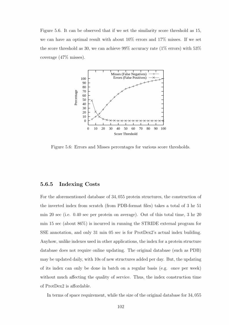
Figure 5.6. It can be observed that if we set the similarity score threshold as 15,

we can have an optimal result with about 10% errors and 17% misses. If we set

the score threshold as 30, we can achieve 99% accuracy rate (1% errors) with 53%

coverage (47% misses).

0102030405060708090

100

0 10 20 30 40 50 60 70 80 90 100

Perc

enta

ge

Score Threshold

Misses (False Negatives)Errors (False Positives)

Figure 5.6: Errors and Misses percentages for various score thresholds.

5.6.5 Indexing Costs

For the aforementioned database of 34, 055 protein structures, the construction of

the inverted index from scratch (from PDB-format files) takes a total of 3 hr 51

min 20 sec (i.e. 0.40 sec per protein on average). Out of this total time, 3 hr 20

min 15 sec (about 86%) is incurred in running the STRIDE external program for

SSE annotation, and only 31 min 05 sec is for ProtDex2’s actual index building.

Anyhow, unlike indexes used in other applications, the index for a protein structure

database does not require online updating. The original database (such as PDB)

may be updated daily, with 10s of new structures added per day. But, the updating

of its index can only be done in batch on a regular basis (e.g. once per week)

without much affecting the quality of service. Thus, the index construction time

of ProtDex2 is affordable.

In terms of space requirement, while the size of the original database for 34, 055

102

proteins in PDB format (3D coordinates only, without annotations) is 6.17 GB,

that of the entire inverted index is only 51.8 MB (i.e. less than 1% of the original

database’s size).

5.7 Conclusion

In this chapter, we have proposed a new SSE-based indexing scheme for efficient

retrieval of protein structures from the large databases. We conducted an experi-

ment on the retrieval efficiency and effectiveness of the scheme in comparison with

the other methods by using a small database and some query proteins from the

well-known Globins and Serine/Threonin Kinases SCOP Families. We also con-

ducted another experiment using a larger database and several query proteins from

diverse SCOP Families so as to observe the more general behavior of the scheme.

The experimental results showed that our method is very much faster than

two popular protein structure comparison methods, DALI and CE, yet not much

sacrificing on the accuracy of the comparison. When comparing with an SSE-based

database scan method, Topscan, our scheme is much faster even with a slightly

better accuracy. In filter-and-refine framework, it can be ideally used as a filtering

tool to reduce the search space before running a slow detailed structural comparison

method.

Finally, it can become a very useful scheme in the near future when the protein

structure database sizes become too large to be searched through exhaustively.

103

CHAPTER 6

Protein Structure Classification

Summary

In this chapter, we present a new scheme named “ProtClass” for automatic clas-

sification of 3D protein structures. It is a dedicated and unified multi-class clas-

sification scheme. Neither detailed structural alignment nor multiple binary clas-

sifications are required in this scheme. We adopt a nearest-neighbor classification

strategy with a filter-and-refine scheme. In the first step, we filter out the most

improbable by a coarse search. In the second, we perform a relatively more detailed

search on the remaining answers. We also incorporate the pre-learned parameters

from the training data in searching the nearest neighbors. We employ very concise

and effective encoding schemes of the 3D protein structures in both steps. We

compare our proposed method against two other dedicated protein structure clas-

sification schemes, namely SGM [RF03] and CPMine [AT04a]. The experimental

results show that ProtClass is slightly better in accuracy than SGM, and much

faster than it. In comparison with CPMine, ProtClass is much more accurate,

while their running times are about the same. We also compare ProtClass against

a detailed structural alignment-based classification scheme named DALI [HS93],

which is found to be slightly more accurate, but extremely slower.

104

6.1 Introduction

Categorization of protein structures allows us to study the structural properties of

proteins more easily through reductionism. Other benefits of structural categoriza-

tion include provision of knowledge on sequence–structure relationships, reduction

of search space functional prediction, etc. [Bou05, Ore99]. Protein structure cate-

gorization encompasses two different yet related topics: (1) clustering or building

structural groups (classes) of proteins from scratch, and (2) classification or adding

a new protein into the most appropriate of the existing structural classes.

We will study the automatic classification of protein structures in this chapter.

In order to build an automatic classifier, we must have a database of protein

structures whose class labels — in terms of a standard (usually a manual) class

annotation system such as SCOP [HAB+97] and CATH [OMJ+97] — are already

known. We use this database as the training data for the classifier. The classifier

learns the relationships between the structural properties of the proteins and their

structural class labels, and stores this knowledge in some abstract form. When

a new protein (a query) is to be classified, the classifier reapplies the learned

knowledge to predict its structural class label.

As discussed in Section 1.1.3, nearest neighbor, support vector machines, de-

cision trees, hidden Markov model and fingerprinting are the methods for protein

structure classification (and classification in general as well). Nearest neighbor

classification is the most common used method for structural classification. Any

detailed or coarse structural alignment tool or any explicit index-based search

method can be used to find the protein(s) in the database that is/are most similar

to the query, and derive the query’s class label from its/their label(s).

Nearest neighbor classification is simple and generally effective. But it is gen-

erally inefficient — particularly in the present age of large structural databases. In

addition, it usually lacks an active learning, and hence, fails to exploit the knowl-

edge of the existing classes (unlike other classification methods such as support

vector machines).

In this chapter, we propose a new protein structure classification system named

105

ProtClass (Protein Classification), which rectifies the above weaknesses of the

traditional nearest neighbor systems. Our objective is to develop an efficient and

effective learning-based nearest neighbor classifier that do not have to perform any

detailed structural comparison/alignment.

Suppose we have a database (training data) of protein structures together with

their SCOP class labels. We train our classifier by encoding each protein structure

in a concise format with two levels of abstraction, and extracting some important

pieces of information from each distinct class. In this way, we can explore the

prior knowledge of human expert judgement in classifying protein structures, and

exploit this knowledge for classifying the new proteins in the future.

When we want to classify a query protein structure whose class is not known

yet, we also represent it in its concise format, and conduct a filter-and-refine search.

Firstly, we filter out the database proteins which are quite unrelated to the query

using the first-level abstract representation. Secondly, for refinement, we employ

a more detailed nearest-neighbor search based on the second-level abstract repre-

sentation. In the both steps, we utilizes the pre-learned parameters of the distinct

classes. Finally, we report the class label(s) of the nearest neighbor protein(s) as

the possible class designation(s) for the query.

6.2 Encoding Protein Structures

In this section, we will discuss how ProtClass concisely and effectively represents

a 3D protein structure in its encoded formats, namely PA and CPset ; and how it

measures the similarities between these encoded structures.

6.2.1 Protein Abstract (PA)

Let P be a 3D protein structure. Let A = a1a2a3 . . . a|A| be the amino acid

(AA) residue sequence of P where |A| is the number of residues in P . Let S =

s1s2s3 . . . s|S| be the SSE sequence of P where |S| is the number of SSEs in P . As

an example, let us assume we have a 10 residue protein P with the following AA

106

sequence A.

K F A V N H I T R S

Let us also assume that we have 3 SSEs in the protein where residue 2–3 forms a

sheet, 5–6 a helix, and 8–10 a sheet. Then we have the SSE sequence S of P as

follows.

E H E

Here we formulate a concise encoding format named Protein Abstract (PA).

It is a simple tuple featuring 6 attributes regarding the overall structure of a 3D

protein structure as shown in Table 6.1.

Table 6.1: Attributes in a Protein Abstract (PA).

Sr Description Symbol Equation Example for

protein P

1 No. of AA residues |A| 10

2 No. of SSEs |S| 3

3 Total length of all SSEs as SL (6.1) 0.7

a percentage of no. of residues

4 Total length of all helices as HL (6.2) 0.29

a percentage of total SSE length

5 No. of helices as HN (6.3) 0.33

a percentage of no. of SSEs

6 SSE sequence S E H E

Attribute no. 1, 2 and 6 are readily available from the PDB file and the STRIDE

output. Attribute no. 3–5 can be calculated using the following equations.

SL = (

|S|∑i=1

|si|) / |A| (6.1)

where |si| is the length of SSE si. Here, the length of an SSE is an integer in

terms of the number of AA residues it constitutes (rather than its physical length

107

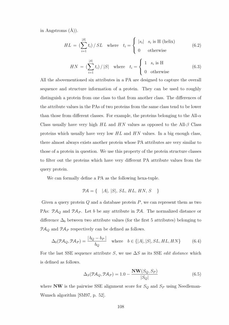
in Angstroms (A)).

HL = (

|S|∑i=1

ti) / SL where ti =

|si| si is H (helix)

0 otherwise(6.2)

HN = (

|S|∑i=1

ti) / |S| where ti =

1 si is H

0 otherwise(6.3)

All the abovementioned six attributes in a PA are designed to capture the overall

sequence and structure information of a protein. They can be used to roughly

distinguish a protein from one class to that from another class. The differences of

the attribute values in the PAs of two proteins from the same class tend to be lower

than those from different classes. For example, the proteins belonging to the All-α

Class usually have very high HL and HN values as opposed to the All-β Class

proteins which usually have very low HL and HN values. In a big enough class,

there almost always exists another protein whose PA attributes are very similar to

those of a protein in question. We use this property of the protein structure classes

to filter out the proteins which have very different PA attribute values from the

query protein.

We can formally define a PA as the following hexa-tuple.

PA = |A|, |S|, SL, HL, HN, S

Given a query protein Q and a database protein P , we can represent them as two

PAs: PAQ and PAP . Let b be any attribute in PA. The normalized distance or

difference ∆b between two attribute values (for the first 5 attributes) belonging to

PAQ and PAP respectively can be defined as follows.

∆b(PAQ,PAP ) =| bQ − bP |

bQwhere b ∈ |A|, |S|, SL,HL,HN (6.4)

For the last SSE sequence attribute S, we use ∆S as its SSE edit distance which

is defined as follows.

∆S(PAQ,PAP ) = 1.0− NW(SQ, SP )

|SQ|(6.5)

where NW is the pairwise SSE alignment score for SQ and SP using Needleman-

Wunsch algorithm [SM97, p. 52].

108

Suppose we have the pre-calculated difference (or distance) threshold values δb

for all the 6 PA attributes. (The threshold value for each attribute is different from

class to class. We will discuss how to calculate these threshold values for each of

the distinct classes from the training data in Section 6.3.1.) When comparing a

pair of PAs (one from Q and one from P ), they are deemed similar if and only if

∆b ≤ δb for every b. The similarity between two PAs can be formally defined as:

Similar(PAQ,PAP , δ) =

TURE if ∆b(PAQ,PAP ) ≤ δb

for ∀ b ∈ |A|, |S|, SL,HL,HN, S

FALSE otherwise

(6.6)

where δ is the set of PA attributes’ distance thresholds for the class to which the

database protein P belongs.

After we have determined that a pair of PAs is similar, we can calculate the

overall distance PADist between them as a simple Euclidean distance as follows.

(We do not have to calculate PADist for the two PAs that are not similar. On

average, for a PA of a query protein, about 71% of the PAs in the database are

dissimilar and can be discarded right away.)

PADist(PAQ,PAP , δ) = (∑

b∈|A|,|S|,SL,HL,HN,S

(∆b(PAQ,PAP )

δb)2 )0.5 (6.7)

in which dividing the actual distance ∆b with distance threshold δb maps the nor-

malized distance into the range of 0 to 1 for all attributes. We assume equal weights

for all the attributes.

Now, we can derive the matching score PAMatch between two PAs as based on

PADist :

PAMatch(PAQ,PAP , δ) =

√6− PADist(PAQ,PAP , δ)√

6(6.8)

where√6 is the maximum possible Euclidean distance between two PAs, since a

PA has 6 attributes whose values are between 0 and 1.

PA representation is simple yet powerful. As discussed later, it helps improve

both the efficiency and effectiveness of the scheme. A similar concept of repre-

senting a protein structure in a concise high-level format was also put forward

in [HSZK03].

109

6.2.2 Discrete Contact Pattern Feature Vector Set (CPset)

In this sub-section we will discuss how a 3D protein structure can be represented

as another abstract structure called CPset, which is a set of integer-valued contact

pattern feature vectors.

Contact Pattern (CP) Feature Vector

As discussed in Sections 5.3.1 and 5.3.2 of the ProtDex2 method, we can represent

a 3D protein structure as a 2D distance matrix; define contact patterns (CPs);

and represent them as feature vectors. Here we use a similar feature vector rep-

resentation with 10 attributes (instead of 8 attributes as in ProtDex2) as given in

Table 6.2. The two additional attributes are marked with asterisks. (In fact, we

first tried these two attributes in ProtDex2. But they did not help improve its

accuracy, and we later dropped them from it.)

The two new attributes AS (starting position of sa in AA sequence) and AD

(difference between starting positions of sa and sb in AA sequence) are defined as:

AS = sstarta (6.9)

AD(sa, sb) = sstartb − sstarta (6.10)

where sstarta and sstartb are the starting positions of sa and sb respectively in AA

sequence A. Since b > a, sstartb > sstarta .

The equations for the other attributes can be referred to in the previous chapter.

Now we can define the CP feature vector Kab for CP Cab as:

Kab = ( CT (sa, sb), AS(sa), SS(sa), AD(sa, sb), SD(sa, sb),

Ω(Va,Vb), ND(Va,Vb), V D(Va,Vb),

MD(sa, sb), CD(sa, sb) )

(6.11)

Discrete CP Feature Vector

Now, we encode/discretize the CP feature vector so that it can be represented as

a compact 4-byte integer value. In order to do this, we map each attribute value

110

Table 6.2: Attributes of CP feature vector for ProtClass.

Sr. Attribute Sym Equa Upper Discret

-bol -tion Bound -ization

Bins Bits

1 Type of Cab CT (5.1) 3 4 2

2* Starting position of sa in AA AS (6.9) 800 2 1

sequence A

3 Position of sa in SSE sequence S SS (5.2) 48 12 4

4* Starting position difference AD (6.10) 800 4 2

of sa and sb in AA sequence A

5 Position difference of SD (5.3) 48 20 5

sa and sb in SSE sequence S

6 Torsion angle between Va and Vb Ω [Sfy04] 360.0 16 4

(−180.0 to +180.0)

7 Closest segment–segment distance ND [Sun04] 64.0 16 4

of Va and Vb

8 Nearest vertex pair distance V D (5.6) 64.0 4 2

of Va and Vb

9 Mean of Cα–Cα distances in Cab MD (5.7) 64.0 4 2

10 Contact density of Cab CD (5.8) 1.0 2 1

Total 27

in the feature vector into a discrete number of bins, and concatenate all the bits

representing these bins into a bit string which can naturally be interpreted as an

integer. (The idea of discretization is similar to that of ProtDex2 in the previous

chapter. But, discretization here is done by physical encoding and no hash table

is used as in ProtDex2.)

The objectives of this encoding are (1) to enable efficient handling of the CP

feature vectors, and (2) to allow approximate matching of the original CP feature

111

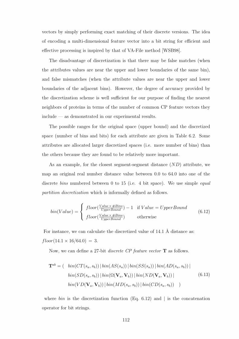
vectors by simply performing exact matching of their discrete versions. The idea

of encoding a multi-dimensional feature vector into a bit string for efficient and

effective processing is inspired by that of VA-File method [WSB98].

The disadvantage of discretization is that there may be false matches (when

the attributes values are near the upper and lower boundaries of the same bin),

and false mismatches (when the attribute values are near the upper and lower

boundaries of the adjacent bins). However, the degree of accuracy provided by

the discretization scheme is well sufficient for our purpose of finding the nearest

neighbors of proteins in terms of the number of common CP feature vectors they

include — as demonstrated in our experimental results.

The possible ranges for the original space (upper bound) and the discretized

space (number of bins and bits) for each attribute are given in Table 6.2. Some

attributes are allocated larger discretized spaces (i.e. more number of bins) than

the others because they are found to be relatively more important.

As an example, for the closest segment-segment distance (ND) attribute, we

map an original real number distance value between 0.0 to 64.0 into one of the

discrete bins numbered between 0 to 15 (i.e. 4 bit space). We use simple equal

partition discretization which is informally defined as follows.

bin(V alue) =

floor(V alue×#BinsUpperBound

)− 1 if V alue = UpperBound

floor(V alue×#BinsUpperBound

) otherwise(6.12)

For instance, we can calculate the discretized value of 14.1 A distance as:

floor(14.1× 16/64.0) = 3.

Now, we can define a 27-bit discrete CP feature vector T as follows.

Tab = ( bin(CT (sa, sb)) | bin(AS(sa)) | bin(SS(sa)) | bin(AD(sa, sb)) |

bin(SD(sa, sb)) | bin(Ω(Va,Vb)) | bin(ND(Va,Vb)) |

bin(V D(Va,Vb)) | bin(MD(sa, sb)) | bin(CD(sa, sb)) )

(6.13)

where bin is the discretization function (Eq. 6.12) and | is the concatenation

operator for bit strings.

112

CPset

Now, we can encode an entire 3D protein structure as a set of discrete CP feature

vectors it contains. We call this set a CPset, and denote it as CPS. CPSP of protein

structure P with |S| SSEs can be defined as:

CPSP = T12, T13, . . . ,T1|S|, T23, . . . ,T(|S|−1) |S| (6.14)

where Tij (where 1 ≤ i ≤ (|S| − 1) and (i+1) ≤ j ≤ |S|) is a discrete CP feature

vector.

The cardinality of a CPset with |S| SSEs is at most |S|(|S| − 1)/2 = O(|S|2).

(There may be some outlier CPs which are excluded from the CPset.)

We sort the discrete CP feature vectors (which can be regarded as integers)

in the CPset in ascending order to enable linear-time comparison of them in the

later classification step. Sorting alters the original order of these discrete feature

vectors in the CPset. However, since the discretized attributes AS (position of

first SSE in AA sequence), SS (position of first SSE in SSE sequence), AD (AA

position difference between first and second SSEs), and SD (SSE position difference

between first and second SSEs) are stored in the discrete CP feature vector, the

positions and relative order of the original CPs in the distance matrix can still be

roughly known.

We can calculate the matching score between two CPsets CPSQ and CPSP with

a simple linear-time algorithm described in Figure 6.1. It is based on the merging

algorithm for two sorted arrays. Being a linear-time algorithm working on integers,

it is very fast.

Both PA and CPset are compact and efficient means of encoding a 3D protein

structure. The average sizes of a PA and a CPset are 160 and 782 bytes respectively,

whereas the average size of an original PDB format file (3D coordinates only,

without any annotation) is about 261 KB (261, 000 bytes).

113

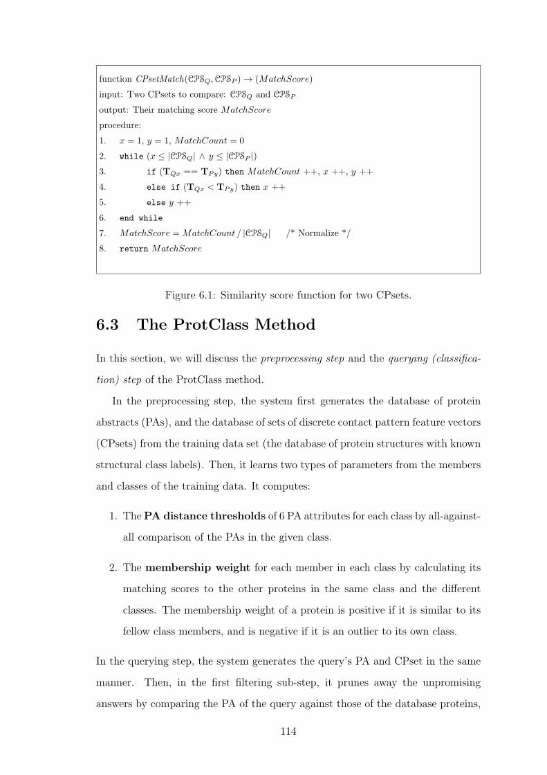
function CPsetMatch(CPSQ,CPSP )→ (MatchScore)

input: Two CPsets to compare: CPSQ and CPSP

output: Their matching score MatchScore

procedure:

1. x = 1, y = 1, MatchCount = 0

2. while (x ≤ |CPSQ| ∧ y ≤ |CPSP |)3. if (TQx == TPy) then MatchCount ++, x ++, y ++

4. else if (TQx < TPy) then x ++

5. else y ++

6. end while

7. MatchScore = MatchCount / |CPSQ| /* Normalize */

8. return MatchScore

Figure 6.1: Similarity score function for two CPsets.

6.3 The ProtClass Method

In this section, we will discuss the preprocessing step and the querying (classifica-

tion) step of the ProtClass method.

In the preprocessing step, the system first generates the database of protein

abstracts (PAs), and the database of sets of discrete contact pattern feature vectors

(CPsets) from the training data set (the database of protein structures with known

structural class labels). Then, it learns two types of parameters from the members

and classes of the training data. It computes:

1. ThePA distance thresholds of 6 PA attributes for each class by all-against-

all comparison of the PAs in the given class.

2. The membership weight for each member in each class by calculating its

matching scores to the other proteins in the same class and the different

classes. The membership weight of a protein is positive if it is similar to its

fellow class members, and is negative if it is an outlier to its own class.

In the querying step, the system generates the query’s PA and CPset in the same

manner. Then, in the first filtering sub-step, it prunes away the unpromising

answers by comparing the PA of the query against those of the database proteins,

114

using the PA distance thresholds learned in the preprocessing step. Then, in

the refinement sub-step, the system conducts a nearest-neighbor search of the

query’s CPset against the remaining database proteins’ CPsets, and returns the

class label(s) of the protein(s) that are best matched. The membership weights

learned from the preprocessing step are also taken into account in selecting the

candidate nearest neighbors.

The overview of the method is illustrated in Figure 6.2. The algorithmic details

of the preprocessing and querying steps are described in the following two sub-

sections.

CP

sets w

ith class labels

Protein

Abstracts

with class labels

Extract Protein

Abstracts

CPset representation

Prepare Protein Abstract & CPset

Nearest neighbor search on CPsets

Find class parameters

Param

eters for each

class

Filter proteins

Preprocessing Step Querying (Classification) Step

3D protein

structures w

ith class labels

Query protein with unknown class label

Figure 6.2: Overview of ProtClass method.

6.3.1 Preprocessing Algorithm

Given a database of protein structures with known class labels, we can generate the

databases of PAs, CPsets, and the two class parameters using the preprocessing

algorithm shown in Figures 6.3 and 6.4. For each distinct class, we generate the

115

PAs and CPsets for the proteins belonging to this class, and store them in the

database (line 4–10).

We calculate the membership weight for each protein with respect to its class

(line 15). We use the silhouette width measure [KR90] for the membership weight.

For a protein j in class i, its silhouette width is defined as:

SilhouetteWidth(i, j) =b(j)− a(j)

max(a(j), b(j))(6.15)

where a(j) is the average distance of j to its fellow class members in class i, and

b(j) is the average distance of j to the members in its nearest neighbor class other

than i. The distance between two proteins Q and P is calculated based on their

PA matching score and CPset matching score as follows:

Dist(Q,P ) = 1.0− (PAMatch(PAQ,PAP , δdefault) · CPsetMatch(CPSQ,CPSP ))

(6.16)

where PAMatch and CPsetMatch are defined in Equation 6.8 and Figure 6.1 re-

spectively. δdefault is described in the last paragraph of the current sub-section.

In calculating the silhouette width, if b(j) > a(j), the result will be a positive

value. Otherwise, it will be a negative value. In other words, if a member protein

in a class is closer to its fellow members than to the members in other class, its

membership weight (silhouette width) will be positive, This protein is useful in

predicting the class of a query protein by nearest neighbor search in the future.

On the other hand, if a member protein is closer to the members of other classes

than to its own fellow members, it is an outlier and its membership weight will be

negative. This protein should not be taken into account in determining the nearest

neighbor of the query protein. The use of membership weights can help improve

the accuracy of classification [BM03].

Again, for each class, we calculate the farthest PA attribute distances maxδb

that are exhibited in the PA pairs belonging to this class. (line 18–21). For each

PA attribute, its farthest distance value is multiplied with a CoverageFactor to

obtain the distance threshold value of this attribute (line 25).

The empirically determined value, CoverageFactor = 0.80, is used in our im-

116

plementation. The objective of setting the threshold distances is to ensure that at

least one nearest proteins belonging to the same class as a given query protein will

pass the filtering step (see the next sub-section), whilst the dissimilar proteins are

discarded straight away. It means that for each PA attribute, we expect to find

the nearest neighbor(s) to a query protein within 80% of the distance of the two

farthest proteins (with respect to this attribute) belonging to this particular class

in the existing database. If the number of trained proteins in a class is too few (say

less than 20), this condition may not be always true. We use the default threshold

values δdefault ≡ (δ|A| = 0.4, δ|S| = 0.4, δSL = 0.3, δHL = 0.2, δHN = 0.3, δS = 0.5)

in this case.

6.3.2 Querying Algorithm

The algorithm in Figure 6.5 describes how unpromising answers with respect to a

given query can be filtered out using PAs, and how the class of the query protein

can be predicted by using the nearest-neighbor search based on the PA similarity

and the CPset similarity, together with the membership weights.

First of all, if the membership weight of a particular member protein in a class

is negative, it is regarded as an outlier, and is neglected in selecting the query’s

nearest neighbors (line 9–10).

In the filtering step, the algorithm first filters out the unpromising answers

using the PA of the query and those of the database proteins (line 11–12). For a

protein that passes the filtering test, the matching score of its PA to the query PA

(PAScore) is calculated (line 13).

Our experimental results show that an average of 71% of the database proteins

are discarded in the filtering step, as they are not close enough to the query.

An average of 38% of the classes are entirely discarded. It should be noted that

the proteins that are in the same class as the query but not similar enough (the

distantly related ones) are also discarded. But the similar ones in the correct class

pass the test. So, there is no chance of discarding the correct class as a whole.

In the second refinement step, the matching score of the protein’s CPset to that

117

function ProtClass Preprocess (D)→ (PA,CPS, δ,MW)

input: Protein structure database D = D1, D2, . . . ,Dn where Di (1 ≤ i ≤ n)

is a set of protein structures with class label i

output: (1) PA database PA = PA1, PA2, . . . ,PAn where PAi (1 ≤ i ≤ n)

is a set of Protein Abstracts for proteins with class label i

(2) CPset database CPS = CPS1, CPS2, . . . ,CPSn where CPSi (1 ≤ i ≤ n)

is a set of CPsets for proteins with class label i

(3) PA distance threshold database δ = δ1, δ2, . . . , δn where δi (1 ≤ i ≤ n)

is a set of PA distance thresholds in class i

(4) Membership weight database MW = MW1, MW2, . . . ,MWn where MWi (1 ≤ i ≤ n) is a set of weights for members in class i

procedure:

1. PA = ϕ, CPS = ϕ, δ = ϕ, MW = ϕ

2. for i = 1 to n /* n is the number of distinct classes */

3. PAi = ϕ, CPSi = ϕ, δi = ϕ, MWi = ϕ

4. for j = 1 to |Di| /* |Di| is the number of members in class i */

5. Let Dij (1 ≤ j ≤ |Di|) be an individual protein structure in Di

6. PAij = GeneratePA(Dij) /* See Section 6.2.1 */

7. PAi = PAi ∪ PAij

8. CPSij = GenerateCPset(Dij) /* See Section 6.2.2 */

9. Sort(CPSij) /* Sort in ascending order */

10. CPSi = CPSi ∪ CPSij

11. end for

(continued to Figure 6.4)

Figure 6.3: ProtClass preprocessing algorithm.

of the query (CPsetScore) is calculated is using the function CPsetMatch (line

15). Since the function is a linear-time algorithm and it only has to handle integer

values, the calculation is very fast. The final score of the protein with respect

to the query is calculated by taking both its PA matching score (PAScore) and

CPset matching score (CPsetScore) into account (line 16). Finally, we return the

class label of the protein which is the nearest to the query (in terms of the final

score), and optionally other information such as the best scoring protein for each

class, etc. (line 23).

118

(continued from Figure 6.3)

12. for each b ∈ |A|, |S|, SL,HL,HN,S /* b is a PA attribute */

13. maxδb = 0

14. for j = 1 to |Di| /* |Di| is the number of members in class i */

15. MWij = SilhouetteWidth(i, j) /* Eq. 6.15 */

16. MWi = MWi ∪MWij

17. for k = 1 to |Di|18. for each b ∈ |A|, |S|, SL,HL,HN,S19. if (maxδb < ∆b(PAij ,PAik)) then

20. maxδb = ∆b(PAij ,PAik) /* Eq. 6.4 and 6.5 */

21. end for

22. end for

23. end for

24. for each b ∈ |A|, |S|, SL,HL,HN,S25. δib = maxδb × CoverageFactor

26. δi = δi ∪ δib

27. end for

28. PA = PA ∪ PAi, CPS = CPS ∪ CPSi, δ = δ ∪ δi, MW ∪MWi

29. end for /* of line 2 */

30. return (PA,CPS, δ,MW)

Figure 6.4: ProtClass preprocessing algorithm (contd.).


In order to assess the accuracy and efficiency of the proposed ProtClass scheme,

we test it on a medium size data set with 600 protein structure in the experimen-

tal setup mentioned below. We compare ProtClass against DALI [HS93] (using

DaliLite [HP00] implementation), SGM [RF03] and CPMine [AT04a] using their

default settings in the same experimental setup. When running DaliLite, we use

its database search option rather than its pairwise alignment option.

119

function ProtClass Query (Q,PA,CPS, δ,MW)

→ ((MaxClass,MaxClassScore), (MaxProtein,MaxScore))

input: (1) Query protein structure Q

(2) PA,CPS, δ,MW /* See their definitions in above algorithm Figure 6.3. */

output: (1) Most possible class MaxClass for Q and its score MaxClassScore

(2) Most possible proteins MaxProtein and their respective scores MaxScore

arrays for all distinct classes /* optional */

procedure:

1. PAQ = GeneratePA(Q) /* See Section 6.2.1 */

2. CPSQ = GenerateCPset(Q) /* See Section 6.2.2 */

3. Sort(CPSQ) /* Sort in ascending order */

4. Let CPSQ = TQ1, TQ2, . . . ,TQ |CPSQ| where TQx (1 ≤ x ≤ |CPSQ|)is a discrete CP feature vector of Q.

5. MaxClassScore = 0, MaxClass = 0

6. for i = 1 to n /* n is the number of distinct classes */

7. MaxScorei = 0, MaxProteini = 0

8. for j = 1 to |PAi| /* |PAi| is the number of trained proteins in class i */

9. if (MWij ≤ 0 ) then /* Check if membership weight is negative */

10. continue; /* outlier of its own class; skip this protein */

11. if ( Similar(PAQ, PAij , δi) == FALSE ) then /* See Eq. 6.6 */

12. continue; /* filter test failed; skip this protein */

13. PAScore = PAMatch (PAQ, PAij , δi) /* See Eq. 6.8 */

14. Let CPSij = TP1, TP2, . . . ,TP |CPSij | where TPy (1 ≤ y ≤ |CPSij |)is a discrete CP feature vector of CPSij .

15. CPsetScore = CPsetMatch (CPSQ,CPSij) /* See Fig. 6.1 */

16. FinalScore = PAScore× CPsetScore

17. if (FinalScore > MaxScorei ) then

18. MaxScorei = FinalScore, MaxProteini = j

19. end for

20. if (MaxScorei > MaxClassScore ) then

21. MaxClassScore = MaxScorei, MaxClass = i

22. end for

23. return ((MaxClass, MaxClassScore), (MaxProtein, MaxScore))

Figure 6.5: ProtClass querying (classification) algorithm.

6.4.1 Experimental Setup

We use the ASTRAL data set [BKL00] that contains proteins with less than 40%

sequence homology. From this data set, we choose 15 “Folds” (according to SCOP

120

designation) each with 40 member proteins. (For Folds with more than 40 mem-

bers, we randomly select 40 from them.) Thus, we have a pool of 15 × 40 = 600

protein structures whose class labels (Folds) are known. We use these 15 Folds as

our target structural classes.

We conduct our experiment using 10-fold cross validation strategy. We split

each Fold into 10 partitions each having 4 protein structures. We conduct 10 sub-

experiments in each of which we build the testing data set by choosing a partition

from each of the Folds and combining them together. In this way, we have a

testing data set consisting of 60 proteins for each sub-experiment. The remaining

540 proteins are used as the training data set. The training data set is made up of

36 proteins from each of 15 Folds.

In other words, in each sub-experiment, we have a database of 540 protein

structures whose Folds are already known, and a set of 60 query protein structures

whose Folds are to be predicted. We then validate the predicted Folds of the query

proteins against their actual Folds as designated by SCOP.

6.4.2 Accuracy

In the abovementioned manner, 10 sub-experiments are conducted by using the

different testing sets and training sets in each cycle. Then, we consolidate the

results from 10 sub-experiments and calculate the average accuracy of the scheme.

We look at the top 3 scoring Folds (which is 20% of the total number of distinct

Folds), and examine whether they are actually the correct classifications. The

results are shown in Table 6.3. Column “Top 1” shows the accuracy of the scheme

if only the topmost scorer is examined, and Column “Top 2” shows the accuracy

if both top 1 and 2 scorers are examined, etc. The accuracy results of DALI, SGM

and CPMine are also shown in Table 6.3.

With a large number of possible classes (15 SCOP Folds in this case), it may

be more useful to report a few candidate classes rather than reporting a single

but incorrect class — as long as the number of reported classes is only a small

fraction of all the possible classes (20% in our case). The user can manage these

121

candidate classes according to his/her own requirement. For example, if only

moderate accuracy in classification is required, the user can just take the topmost

scoring class as the answer. If high accuracy is needed, manual inspections or

detailed structural alignments can be done on the top scoring members of the top

3 scoring classes. This strategy of reporting more than one class as the possible

candidates is also advocated by the authors of SGM [RF03].

From the experiments, it is observed that ProtClass performs quite accurately.

In overall, it offers an average accuracy of 99.17% if we take the top 3 scorers into

account and 91.17% if we take only the topmost scorer into account.

It gives the perfect results on certain Folds such as 47472, 48370, and 51734

with 100% accuracy even with the topmost scorer. It performs quite fairly on

certain Folds such as 52171 (95% accuracy with the top 3 scorers and 85% with

the topmost scorer).

As expected, DALI exhibits more accuracy than ProtClass. Its high accuracy

(99.7% with the topmost and 99.2% with top 3) can be attributed to its detailed

structural alignment mechanism. But, on the other hand, this approach is ex-

tremely slow (see Section 6.4.3). We can achieve the same high accuracy as DALI

while reducing the running time by employing ProtClass as a rapid query prepro-

cessor. We can run the filtering step of ProtClass before running DALI itself. The

filtering step filters out the about 71% of all the database proteins as irrelevant.

It is observed that the proteins that are relevant to the final answer are always re-

tained in the remaining 29% to be processed by DALI in the next step. Therefore

we do not miss out anything, but can reduce the total running time by about 73%.

This means 370% improvement in speed.

The overall accuracy of ProtClass is slightly better than that of SGM. Out of

15 Folds tested, ProtClass performs better than SGM in 9 Folds, equally in 5 Folds,

and poorer in 1 Fold (according to the top 3 scorer results). We can observe some

similarities between the result of ProtClass and that of SGM. For example, both

methods give perfect results for Folds 48370, 48725, 51734, etc., but give poor

topmost scorer results for Fold 52439.

122

In comparison with CPMine, ProtClass is found to be much more accurate.

This is because CPMine is a fingerprint-based comparison approach without us-

ing any filters. Matching a query against the fingerprints of the classes (Folds in

this case) can introduce both false positives and false negatives, because the finger-

prints sometimes cannot represent their respective classes uniquely and unfailingly.

In ProtClass, we do not use such a fingerprinting mechanism, thus reducing the

possibility of false classifications due to misrepresentation.

6.4.3 Speed

It is observed that the proposed ProtClass scheme works very efficiently. All the

experiments are done on Sun Ultra Sparc II with two 480MHz CPUs and 4GB

main memory, running Sun OS 5.7. The time statistics are shown in Table 6.4.

It shows the time taken to run one cycle of sub-experiment (preprocessing on 540

proteins, and querying with 60 proteins) by each method. It is averaged out from

the times taken by the 10 sub-experiments in 10-fold cross validation.

Although DALI is more accurate than ProtClass, it is found to be about 620

times slower! It takes an average of about 1 day and 21 hours for querying of 60

proteins on the database of 540 proteins. In fact, it may be impractical to use DALI

for a real-time classification task involving a large database on an average stand-

alone machine. In the previous sub-section, we have already discussed how we can

improve the running time of DALI by using ProtClass as a rapid preprocessor.

In comparison with SGM, it is observed that ProtClass is about 18 times faster.

This is because SGM involves a large number of floating point operations to calcu-

late the Gauss Integrals. On the contrary, ProtClass mainly performs integer and

bit-wise operations. CPMine’s running time is about the same as that of ProtClass.

They both use the similar integer and bit operations.

From the experiment, it is also observed that the running time of ProtClass,

both for preprocessing and querying steps, is overwhelmed by that of STRIDE

external algorithm used to generate the SSE information. The breakdown of the

various time costs in both preprocessing and querying steps are shown in Table 6.5.

123

Tab

le6.3:

Experim

entalresultson

15distinct

Folds.

Fold

Class

Average

Percentage

ofCorrect

Classification

s

DALI

SGM

ProtC

lass

CPMine

Top

1Top

2Top

3Top

1Top

2Top

3Top

1Top

2Top

3Top

1Top

2Top

3

46688

All-α

92.5

95.0

95.0

80.0

95.0

97.5

92.5

97.5

100.0

80.0

85.0

92.5

47472

All-α

100.0

100.0

100.0

80.0

90.0

97.5

100.0

100.0

100.0

47.5

97.5

100.0

48370

All-α

100.0

100.0

100.0

97.5

100.0

100.0

100.0

100.0

100.0

50.0

72.5

85.0

48725

All-β

100.0

100.0

100.0

100.0

100.0

100.0

95.0

97.5

100.0

72.5

97.5

100.0

50198

All-β

100.0

100.0

100.0

82.5

92.5

95.0

90.0

92.5

100.0

30.0

62.5

85.0

51350

α/β

100.0

100.0

100.0

77.5

92.5

97.5

97.5

97.5

100.0

47.5

65.0

77.5

51734

α/β

100.0

100.0

100.0

72.5

95.0

100.0

100.0

100.0

100.0

52.5

85.0

87.5

51904

α/β

100.0

100.0

100.0

97.5

97.5

100.0

95.0

97.5

97.5

32.5

55.0

60.0

52171

α/β

95.0

100.0

100.0

65.0

82.5

82.5

85.0

95.0

95.0

42.5

72.5

95.0

52539

α/β

100.0

100.0

100.0

50.0

72.5

85.0

72.5

90.0

100.0

32.5

60.0

82.5

52832

α/β

100.0

100.0

100.0

90.0

92.5

95.0

95.0

97.5

100.0

25.0

37.5

62.5

53066

α/β

100.0

100.0

100.0

67.5

80.0

92.5

80.0

95.0

95.0

30.0

37.5

47.5

53473

α/β

100.0

100.0

100.0

77.5

92.5

92.5

95.0

97.5

100.0

47.5

60.0

70.0

54235

α+β

100.0

100.0

100.0

87.5

92.5

100.0

85.0

97.5

100.0

50.0

70.0

85.0

54861

α+β

100.0

100.0

100.0

85.0

97.5

100.0

85.0

92.5

100.0

32.5

67.5

90.0

Overall

99.2

99.7

99.7

80.7

91.5

95.7

91.2

96.5

99.2

44.8

68.3

81.3

124

Tab

le6.4:

Average

runningtimes

for60

querieson

540proteinsfor4methods.

Description

Average

timeelap

sed(inseconds)

Average

timeon

oneprotein/q

uery(inseconds)

DALI

SGM

ProtC

lass

CPMine

DALI

SGM

ProtC

lass

CPMine

Preprocessing

1,080

4,297

235

227

2.00

7.96

0.44

0.42

(540

proteins)

Querying

163,466

478

3026

2,724.43

7.97

0.50

0.43

(60proteins)

Total

164,546

4,775

265

253

Tab

le6.5:

Break

dow

nof

costsforProtC

lass

based

onaveragerunningtimes

for60

querieson

540proteins.

Description

Average

timeelap

sed

Average

timeon

one

(inseconds)

protein/q

uery(inseconds)

Preprocessing(540

proteins)

-RunningSTRID

E211.53

0.39

-GeneratingPAs,CPsets,an

dclassparam

eter

datab

ases

23.78

0.04

Total

235.31

Querying(60queries)

-RunningSTRID

E24.05

0.40

-Preparingqueries(PA

andCPset)

1.31

0.02

-Filteringstep

1.94

0.03

-Refinem

entstep

2.85

0.05

Total

30.15

125

6.4.4 Effect of Proportion of Training and Testing Data

In our 10-fold cross validation experiment on 600 proteins, we use 540 (90%) of

them as the training data, and the remaining 60 as the testing data in each cycle.

In order to explore the effect of the proportion of the training and testing data, we

change it variously and observe the changes in the accuracy of the scheme. First,

we conduct the leave-one-out test by using 15 proteins as the testing data (one

from each distinct Fold) and the remaining 585 as the training data, and repeat

the experiment 40 times. In Figure 6.6, the label on x-axis “97.5%” means that

the percentage of the training proteins is 97.5% of the total proteins (i.e. 585 out

of 600). The label “(39/40)” means that 39 out of 40 proteins in each distinct Fold

are used as the training data. The other test cases are with 75%, 50%, and 25%

training data respectively. All these are compared against our default test with

90% training data as shown in the figure.

Similar experiments are also conducted on SGM whose results are also shown

in Figure 6.6. We exclude DALI and CPMine from our experiment, because the

former takes a very long time to run, and the latter is clearly inferior to ProtClass.

As expected, the accuracy of the scheme gradually declines with the reduction

of the training data percentage. However, there are no steep slopes in the curves.

In the worst case with 25% training data, ProtClass can still provide the accuracies

of 77.4%, 88.0%, and 93.2% for the topmost, top 2, and top 3 answers respectively.

We can also observe a similar trend of declining accuracy in the curves of SGM.

In fact, this is a general phenomenon for all classification systems — the more the

training data, the better the accuracy.

6.4.5 Effect of Class Size

In our experiment, we use classes (SCOP Folds) with 40 members each, which can

be considered as relatively “big” ones. In order to assess the performance of the

scheme on the various sizes of Folds, we run multiple tests on various Fold sizes.

In the first test, we take Folds with at least 2 members from ASTRAL data set

with less than 40% sequence homology. (For Folds with more than 2 members, we

126

70

75

80

85

90

95

100

97.5%(39/40)

90%(36/40)

75%(30/40)

50%(20/40)

25%(10/40)

Percentage of Training Data

Ave

rag

e A

ccu

racy

(%

)

SGM (Top1)SGM (Top2)SGM (Top3)ProtClass (Top1)ProtClass (Top2)ProtClass (Top3)

Figure 6.6: Effect of percentage of training data.

randomly choose 2 from them.) There are 350 such Folds, thus yielding a data set

with (350×2 = 700) proteins. Then we run two test cycles, each with 350 training

proteins and 350 testing proteins. The other test cases are for Folds with 5, 10,

15 members etc. up to 50 members. The results are shown in Figure 6.7. Similar

experiments are also conducted on SGM.

ProtClass can only provide 50% accuracy (with the top 3 scorers) for the Folds

with 2 members. However, given a very large number of possible Folds (350), this

50% accuracy is not trivial. We can observe the trend of accuracy improvement

with the increased number of members in the Folds. ProtClass can provide a

reasonable accuracy of at least 80% for the Folds with 10 or more members when

the top 3 scorers are taken into account, and 25 or more members when only the

topmost scorer is taken into account. We can also see a similar trend of accuracy

improvement in the curves of SGM. The accuracy of SGM is better than ProtClass

for 2-member Folds, but the latter is generally better for the rest of the Folds. It is

interesting to observe a high degree of correlation between the curves of ProtClass

and those of SGM.

127

30

40

50

60

70

80

90

100

2 (3

50)

5 (1

65)

10 (9

4)

15 (4

9)

20 (3

9)

25 (2

5)

30 (1

8)

35 (1

5)

40 (1

5)

45 (1

0)

50 (

8)

No. of members in Fold (No. of Folds tested)

Ave

rag

e A

ccu

racy

(%

)

SGM (Top1)SGM (Top2)SGM (Top3)ProtClass (Top1)ProtClass (Top2)ProtClass (Top3)

Figure 6.7: Effect of number of members in each distinct Fold.

6.5 Discussions

6.5.1 Importance of Filter and Refine Steps

With the hope to further improve the accuracy of the scheme, one may be tempted

to drop the filtering step and run only the relatively more detailed refinement step

on every database protein. But, unfortunately, this does not work. The accuracy

of the system degrades substantially if filtering is not carried out. This is because

the filtering step can prune away a lot of potential false positive proteins whose

CPsets are similar to that of the query, but whose PAs are not. Our experimental

results show that both filtering and refinement steps are indispensable. Figure 6.8

shows the overall accuracy of the system when both steps are included, and when

each step is dropped at a time.

6.5.2 Importance of PA Attributes

In order to assess the importance of the six attributes in a PA, we drop each

attribute at a time and re-run the experiment as described in Section 6.4.1. It is

observed that all the attributes are more or less important on their own, because

dropping any of them reduces the accuracy of the scheme — as shown in Figure 6.9.

128

30405060708090

100

Only Filter(withoutRefine)

Without Filter Filter+Refine

Method

Av

era

ge

Ac

cu

rac

y(%

)

Top 3Top 2Top 1

Figure 6.8: Importance of filter and refine steps.

6.5.3 Importance of CP Feature Vector Attributes

Similarly, in order to evaluate the importance of the ten attributes in a CP feature

vector, we exclude each attribute at a time from the experiment as described

in Section 6.4.1. Again, it is found out that all the attributes are more or less

important, because dropping any of them degrades the accuracy of the scheme —

as shown in Figure 6.10. Although all the attributes are important, some attributes

— such as CT (contact pattern type) and Ω (torsion angle) — are found to be

more important than the others, as the exclusion of these attribute affects the

accuracy of the system more seriously. (This observation is consistent with that

on ProtDex2 as discussed in Section 5.6.3 in the previous chapter.)

80

85

90

95

100

None |A

||S

|SL HL

HN S

Excluded PA Attribute

Av

era

ge

Ac

cu

rac

y(%

)

Top 3Top 2Top 1

Figure 6.9: Importance of each PA at-

tribute.

80

85

90

95

100

None CT AS SS AD SD

Omeg

aND VD

MD CD

Excluded CP Feature Vector Attribute

Av

era

ge

Ac

cu

rac

y(%

)

Top 3Top 2Top 1

Figure 6.10: Importance of each CP

feature vector attribute.

129

6.5.4 ProtClass vs ProtDex2

Although ProtClass also uses a CP feature vector representation as in the ProtDex2

method, it is not a trivial extension of ProtDex2. In particular:

1. ProtClass is a two-tier system using the PA representation in the upper tier

and the CPset representation in the lower tier. On the other hand, ProtDex2

is a single-tier system using the hash table of CPs. ProtClass is a filter-and-

refine system whereas ProtDex2 is not one by itself (although it can be used as

a filtering tool in conjunction with any existing detailed comparison method).

2. The scoring function of ProtClass is a coarse one designed just enough to be

able to recognize a few nearest neighbors with respect to the query. Prot-

Dex2’s scoring function is more detailed and designed to identify a number

of proteins that are both closely and distantly related to the query.

3. Being a classification system, ProtClass need to know the class labels of the

database proteins in advance, and utilize these class labels. In contrast, being

a mere database search system, ProtDex2 neither need nor utilize any class

label.

6.6 Conclusion

Nowadays, due to the high throughput methods in 3D protein structure deter-

mination, several tens of new protein structures are deposited into the structural

databases such as PDB. Biologists naturally want to classify these new structures

into their appropriate structural classes. But, both the manual class assignment

systems (such as SCOP) and detailed alignment-based classification systems (such

as DALI) becomes inefficient because of the large volume of the data involved.

Thus, we are in need of a method that can quickly and effectively classify a newly

determined structure into its appropriate structural class.

In this chapter, we have presented a new automatic scheme for protein struc-

ture classification. Our system is a dedicated classifier without requiring a costly

130

structural comparison process. The experimental results shows that our method

is both accurate and efficient. We have proved its usefulness on a data set with

600 proteins belonging to 15 SCOP Folds. It is very much faster than the tradi-

tional structural alignment-based classification with the DALI method whilst only

slightly less accurate. In comparison with two other purpose-built structural clas-

sification systems named SGM and CPMine, our method is much faster as well as

more accurate.

Finally, we believe our scheme can become a useful tool for rapid structural clas-

sification in the age of very large and rapidly growing protein structure databases.

131

CHAPTER 7

Protein–Protein Interface Clustering

Summary

In this chapter, we present a new method to encode, cluster and analyze the similar

3D interface patterns among various protein complexes. We represent the protein–

protein interfaces as 2D residue–residue interface matrices, and encode them as

multi-dimensional feature vectors. Then, we cluster the interfaces using these

feature vectors, and analyze the resultant clusters by various means. Experimental

results show that we can discover a number of statistically significant clusters of

interfaces. A visual inspection also confirms that the interfaces that fall into the

same cluster are visually similar. We can find out the clusters of similar interface

patterns in the protein complexes belonging to diverse structural fold types. We

can also discover in some clusters the recurring interface patterns associated with

biologically important functional motifs. Furthermore, we compare our method

with the sequence-only clustering approach, and observe that ours is much better

in terms of the statistical significance of the resultant clusters.

132

7.1 Introduction

Like structural classification discussed in the previous chapter, structural clustering

is another instance of protein structure categorization. The aim of clustering is to

organize a given set of objects in an orderly manner in such a way that the objects

that are close to each other are in the same clusters, whilst those that are far apart

are in different clusters. By definition, it is unsupervised learning in that we do

not know the class or cluster labels of all the objects a priori ; but rather we try

to generate these labels [HK05].

In protein structure context, we try to organize the protein structures shar-

ing common structural characteristics into their respective clusters. There are

well-established and quite popular clustering methods such as FSSP [HS94a] for

clustering protein chains, and DDD [HS98] for clustering protein domains. There-

fore, we do not intend to build another protein chain or domain clustering system,

but focus on a relatively less studied area of clustering protein–protein interfaces.

Any protein rarely acts alone, but rather interacts with other proteins to per-

form a specific function. The study of protein–protein interactions (PPI) is an

important field in bioinformatics. We can acquire comprehensive knowledge on

the biological functioning of cells by studying the interactions of proteins. This

knowledge can be applied in many real-life applications such as drug discovery.

In this chapter, we study the 3D protein complexes which are formed by the

interactions of proteins. In these complexes, we focus on the regions called protein–

protein interfaces (or simply interfaces) where interacting proteins come in contact.

We propose a method named PICluster (Protein–Protein Interface Clusterer) for

finding the statistically significant clusters (groups) of interfaces.

We represent each interface as a 2D matrix of the center–center distances of

AA residues that are in contact. From all the interfaces available, we choose a

non-redundant set of them based on the sequence identity of their parent proteins.

Then, we represent each non-redundant interface as a multi-dimensional feature

vector based on the frequency of the types of submatrices they contain. The feature

vector representation is designed in such a way that the similarity between the two

133

vectors can well reflect the structural similarity between their original interfaces.

Finally, we cluster (group) these non-redundant interfaces based on their feature

vector similarities.

From this study, we obtain a number of clusters each containing the interfaces

that are structurally similar to each other. We ensure the quality of these clusters

both by means of statistical analysis and visual verification. We also conduct a

biological analysis on the clusters which results in some important findings. We

discover that some interface clusters are strongly associated with the well-known

motifs of important biological functions.

We also discover in many instances that the structurally similar interfaces in

a same cluster sometimes belong to the parent proteins which are structurally

diverse. This may probably be a clue to the existence of similar protein functions

among the various structural fold types, because the interface portion of a protein

is more responsible for its function than its other portions.

In addition, we highlight the usefulness of our method by comparing it against

the clustering of interfaces by the AA sequence information alone. We find out

that our method can detect a large number of clusters that the sequence-based

method fail to detect.

7.2 Definitions

7.2.1 General Definitions

Naturally, the interacting proteins are close to each other in a cell. The co-occurring

interacting proteins are usually collectively crystallized into their 3D formats as a

single group, deposited as a single entity into PDB [BWF+00] database, and given

a unique PDB ID. Such a group of interacting proteins is referred to as a protein

complex. The member proteins of a protein complex are called protein chains or

polymer chains or simply chains. (See Section 2.2 for more details.)

Within a particular complex, each chain is assigned a unique chain ID. Many

of the complexes are made up of only 2 or 3 chains, but some complexes contain a

134

large number of chains up to 60. In a protein complex, any pair of protein chains

that are directly interacting with each other can be referred to as an interacting

pair. For an interacting pair, there usually exists an interface region through which

they actually interact. The chains between which an interface occur are named the

parent chains of that interface.

For example, in Figure 7.1, the protein complex “gamma delta resolvase” is

designated with the PDB ID 2rsl. It has three protein chains which are assigned

the chain IDs A, B, and C. Chain A of 2rsl is referred to as 2rslA, and so on. In

this complex, there are direct interactions between chains A and B, and between

chains B and C respectively. Thus, we have two interacting pairs which can be

denoted as 2rslAB and 2rslBC [TLWN96]. (There is no direct interaction between

chains A and C, and hence, 2rslAC is not an interacting pair.) The interface

for each interacting pair is highlighted in the figure. The interface for 2rslAB is

encoded as I2rsl(A,B), and that of 2rslBC as I2rsl(B,C). A and B are the parent

chains for I2rsl(A,B), and B and C are for I2rsl(B,C).

Figure 7.1: The protein complex

gamma delta resolvase (PDB ID 2rsl)

with three protein chains A, B and C.

Figure 7.2: Example protein complex

p with chains A and B. The dotted

lines means that the two residues are

in contact.

It should be noted that not all the direct protein interactions (and hence the

interfaces) are pairwise in nature. In some protein complexes, there are interface

regions where more than two chains come into contact. However, in our study, we

divide these triple, quadruple, or higher interfaces into multiple pairwise interfaces,

135

for the sake of simplicity.

Now, we will formally define the terms and their symbols that are used through-

out this chapter. We will also illustrate these terms with an example.

7.2.2 Interface

Let p denote a protein complex, and A and B the chains within p. Let r1, . . . , r|A|

be the set of AA residues in A, where r1 is the N-terminus residue and r|A| is the

C-terminus residue. Similarly, let s1, s2, . . . , s|B| be the set of AA residues in B.

Let 3DDist(•, •) be the Euclidean distance function between any two points in 3D

space.

Definition 7.1 Contact of AA residues

A residue ri (1 ≤ i ≤ |A|) from chain A and a residue sj (1 ≤ j ≤ |B|) from

chain B are in contact, if and only if there exists at least one pair of atoms

(u ∈ ri, v ∈ sj) such that 3DDist(u, v) ≤ 5A.

If ri and sj are in contact, it is denoted as Contact(ri, sj). If not, it is denoted

as ¬Contact(ri, sj).

The distance threshold value 5A is also mentioned as a default value in other

studies such as [BDH+03, DBG+03, TLWN96]. Now, let us define an interface

Ip(A,B) between chains A and B of protein complex p as a nonempty set of pairs

as follows:

Ip(A,B) = (ri, sj) | ri ∈ A (1 ≤ i ≤ |A|) and sj ∈ B (1 ≤ j ≤ |B|)

such that Contact(ri, sj) (7.1)

It should be noted that the set Ip(A,B) can be regarded as an interface if and only

if it is nonempty. For interface Ip(A,B), its parent protein chain pair pAB can be

defined as an interacting pair.

136

7.2.3 Interface Fragment

Let Fp(A) be the set of all AA residues from chain A that participate in interface

Ip(A,B). We call Fp(A) an interface fragment which is defined as:

Fp(A) = ri ∈ A | (ri, sj) ∈ Ip(A,B) for any sj ∈ B

Fp(A) is an ordered set in which the member AA residues are arranged by their

positions along its spatial principle component (PC) vector. (Since the residues in

an interface are not always sequential in nature, arranging them by their sequence

order does not always make sense. It is observed that the PC vector ordering gives

more biologically relevant results than the sequential ordering.)

The PC vector is generated by the principle component analysis of the spatial

(x, y, z) coordinates of the member residues in Fp(A). (Principle component anal-

ysis is a process of finding the general orientation of a set of points in a vector

space. The detailed algorithm on it can be found in [MH87].) Now, we can rewrite

Fp(A) as:

Fp(A) = ri1 , ri2 , . . . , ri|Fp(A)| where pos(rik) ≤ pos(rik+1) for 1 ≤ k < |Fp(A)|

where pos(•) is the position of a residue along the PC vector of the interface

fragment it belongs to. For simplicity, we will rewrite Fp(A) again as:

Fp(A) = a1, a2, . . . , a|Fp(A)| where (ak ≡ rik , 1 ≤ k ≤ |Fp(A)|) (7.2)

In the same way, we can also define the interface fragment Fp(B) for chain B as:

Fp(B) = b1, b2, . . . , b|Fp(B)| (7.3)

It should be noted that an interface fragment is not necessarily contiguous, and

the order of residues in it are not always from the N-terminus to the C-terminus.

137

7.2.4 Interface Matrix

Now let us define rd(•, •) as the distance between the centers of two residues

a ∈ Fp(A) and b ∈ Fp(B):

rd(a, b) =

3DDist(a.center, b.center) if 3DDist(a.center, b.center) ≤ 20A

20A otherwise

(7.4)

where a.center is the algebraic mean of the positions of all atoms in residue a, and

b.center that of b. (The distances greater than 20A are considered insignificant

and just rounded off to 20A. This cutoff value is also used in [CKK04].)

Definition 7.2 Interface Matrix

An interface matrix IMpAB representing the interface Ip(A,B) in interacting pair

pAB is a |Fp(A)| × |Fp(B)| matrix in which IMpAB[i, j] ≡ rd(ai, bj) (where 1 ≤

i ≤ |Fp(A)| and 1 ≤ j ≤ |Fp(B)|).

|Fp(A)| × |Fp(B)| can be defined as the interface size of IMpAB.

An interface matrix is different from a normal distance matrix used in the previous

chapters in that (1) it is asymmetrical, and (2) it stores the algebraic center–center

distances of residues, rather than their Cα–Cα distances.

Let IMTpAB be the transposed matrix of IMpAB. We can rewrite IMT

pAB as

IMpBA. The transposed interface matrices are useful, because given two interacting

pairs pAB and qXY , it may be the case that IMqXY is compatible with IMpBA

rather than with IMpAB.

7.2.5 Submatrix

The interface matrix can be cut into several overlapping square submatrices also

known as sliding windows.

138

Definition 7.3 Submatrix

A submatrix SM(i,j)pAB is a square matrix of size w × w whose starting cell is

IMpAB[i, j] of interface matrix IMpAB where (1 ≤ i + w − 1 ≤ |Fp(A)|) and

(1 ≤ j + w − 1 ≤ |Fp(B)|).

Let SMpAB be the submatrix set of IMpAB, i.e. the set of all submatrices that

belong to interface matrix IMpAB.

SMpAB = SM (i,j)pAB | 1 ≤ i ≤ (|Fp(A)|−w+1) and 1 ≤ j ≤ (|Fp(B)|−w+1) (7.5)

The cardinality of submatrix set SMpAB is (|Fp(A)| − w + 1)× (|Fp(B)| − w + 1).

The submatrix distance sd(•, •) between any two submatrices SM1 and SM2

of size w × w can be calculated as:

sd(SM1, SM2) =

√∑wi=1

∑wj=1(SM1[i, j]− SM2[i, j])2

20 · w(7.6)

where 20 ·w =√∑w

i=1

∑wj=1(20− 0)2 is the maximum possible difference between

the two extreme submatrices: one with all 20A’s and one with all 0A’s (although

all 0A’s is actually infeasible in nature). Here sd(•, •) can be regarded as an

Euclidean distance in an (w × w)-dimensional space normalized by the maximum

possible distance in this space. Being based on Euclidean distance, sd(•, •) has

metric properties: isolation, symmetry and triangular inequality.

Now, let us define the representative submatrix set SM′ given a submatrix set

SM and a distance threshold sdt:

SM′ = SMi ∈ SM | sd(SMi , SMj) > sdt for anySMj ∈ SM′ (7.7)

It means that all the members in SM′ are at least sdt distance apart from each

other. So SM′ forms a non-redundant set of submatrices that can roughly represent

the overall distribution of the submatrices in SM.

7.2.6 Nearest-Neighbor Clustering Algorithm

Clustering is an unsupervised machine learning procedure in which we try to gen-

erate the clusters/ groups of objects that are similar according to a particular

139

distance function. The aim of clustering is to put the objects that are close to each

other in the same clusters, whilst those that are far apart in different clusters.

In this study, we use clustering in various places. We use the threshold-based

single-link nearest-neighbor clustering algorithm as described in Figure 7.3. Our

algorithm is inspired by a similar algorithm given in [Dun03]. (However, the two

algorithms use different strategies on deciding the creation of new clusters.)

Given a distance threshold, we find the clusters, each of which contains the

objects with distances among them not greater than the threshold. It is called

nearest-neighbor algorithm because it assigns an object into a cluster to which it

is the nearest. It is called a single-link algorithm because it chooses the nearest

cluster by considering only the nearest member within this cluster (as opposed to

the complete-link or the average-link approaches where all the members in a given

cluster are taken into account [Dun03]).

For every object in the input data set, we allocate it to the cluster in which

its nearest neighbor exists and all the other existing cluster members are also near

enough to it, with regard to the given threshold. If we cannot detect such a cluster,

we create a new cluster with this object as the first member. After allocating all

objects into clusters, we find the cluster medoids. The medoids are the median

objects of the clusters, where the total distance from each medoid to its peer

cluster members is the smallest.

It should be noted that it is a heuristic algorithm, and the result may vary

depending on the ordering of the input objects. The time complexity of the al-

gorithm for O objects is O(|O|2). But, we use some optimizations (such as early

rejection of an object from a cluster by comparing it first to the extreme members

in the cluster, etc.) in order to make it faster. (For simplicity, those optimizations

are not shown in the algorithm.)

7.2.7 Illustration

As an example, let us consider an imaginary protein complex p with two chains A

(with 12 residues represented as black circles) and B (with 17 residues represented

140

function NNCluster(O, d, dt)→ (K,H)

input: (1) A set of objects O = o1, o2, . . . , o|O|(2) Distance function d(•, •)(3) Distance threshold dt

output: (1) A set of clusters K = K1,K2, . . . ,K|K|(2) A set of cluster medoids H = h1, h2, . . . , h|K|

procedure:

/* Find clusters */

1. k = 1 /* initial number of clusters */

2. K1 = o1, K = K13. for i = 2 to |O|4. mind =∞, mink =∞5. for each Kj ∈ K

6. mindist = minx∈Kj (d(oi, x))

7. maxdist = maxx∈Kj (d(oi, x))

8. if (maxdist ≤ dt ∧ mindist < mind) then mind = mindist, mink = j

9. end for

10. if (mind =∞) then Kmink= Kmink

∪ oi /* add into nearest cluster */

11. else

12. k = k + 1 /* increase the number of clusters */

13. Kk = oi, K = K ∪ Kk /* initialize new cluster */

14. end if

15. end for

/* Find cluster medoids */

16. H = ϕ

17. for each Kj ∈ K

18. hj = argminx∈Kj(∑

y∈Kjd(x, y))

19. H = H ∪ hj20. end for

21. return (K,H)

Figure 7.3: Threshold-based nearest-neighbor clustering algorithm.

141

as white circles) as shown in Figure 7.2. That is, A = r1, r2, . . . , r12 and B =

s1, s2, . . . , s17. Suppose a pair of residues connected by a dotted line are in

contact (by Def. 7.1). Then, their interface Ip(A,B), and interface fragments

Fp(A) and Fp(B) will be:

Ip(A,B) = (r1, s1), (r2, s2), (r3, s2), (r3, s3), (r3, s17), . . . , (r11, s12), (r12, s12) and

Fp(A) = r1, r2, r3, r4, r5, r6, r10, r11, r12, Fp(B) = s1, s2, s3, s17, s16, s10, s11, s12

re-written as:

Fp(A) = a1, a2, a3, a4, a5, a6, a7, a8, a9, Fp(B) = b1, b2, b3, b4, b5, b6, b7, b8

Then, their interface matrix IMpAB will be:

IMpAB =

rd(a1, b1) rd(a1, b2) . . . rd(a1, b8)

rd(a2, b1) rd(a2, b2) . . . rd(a2, b8)

......

. . ....

rd(a9, b1) rd(a9, b2) . . . rd(a9, b8)

The interface size of IMpAB is 9× 8 = 72.

Let us define 2× 2 as the submatrix size. Then, the submatrix set SMpAB will

be

SMpAB = SM (1,1)pAB , . . . , SM

(1,7)pAB , . . . , SM

(8,1)pAB , . . . , SM

(8,7)pAB

Its size |SMpAB| = (9− 2 + 1)× (8− 2 + 1) = 56.

As an example, let us choose two submatrices SM(2,3)pAB and SM

(5,1)pAB which re-

spectively are: rd(a2, b3) rd(a2, b4)

rd(a3, b3) rd(a3, b4)

and

rd(a5, b1) rd(a5, b2)

rd(a6, b1) rd(a6, b2)

Then, their submatrix distance sd(•, •) will be:

sd(SM(2,3)pAB , , SM

(5,1)pAB ) =

√(rd(a2, b3)− (a5, b1))2 + . . .+ (rd(a3, b4)− rd(a6, b2))2

7.3 The PICluster Method

In this section, we will describe the detailed procedures we follow in the PICluster

method in order to discover the clusters/groups of similar protein–protein inter-

faces. The three steps undertaken are:

142

1. Selecting representative interfaces from PDB and representing them as inter-

face matrices.

2. Generating feature vectors for the representative interface matrices.

3. Clustering the interface feature vectors (and hence the original interfaces).

Step 1 is illustrated in Figure 7.4. Steps 2 and 3 are illustrated in Figure 7.5. (Step

2 is in turn elaborated in Figure 7.6.)

Protein Complexes

in PDB

12,690 complexes with 45,494 chains

Filter

Candidate Protein

Complexes

5,503 complexes with 17,300 chains and 17,012 interfaces

Cluster by 30% Sequence Identity

Protein Chain

Clusters

1,667 clusters of chains

Prune away Small/ Large Interfaces

Candidate Interfaces

11,558 candidate interfaces

Select Rep. Interfaces

Rep. Interfaces

1,445 rep. interfaces

Generate Rep. Interface Matrices

Rep. Interface Matrices

1,445 rep. interface matrices

Figure 7.4: Generating representative interfaces.

143

Rep. Interface Matrices

1,445 rep. interface matrices

Generate Sub-matrices (Sect. 4.2.1)

Sub-matrices

1,239,147 sub-matrices

Generate Rep. Sub-matrices (Sect. 4.2.1)

Rep. Sub-matrices

279,168 rep. sub-matrices

(original + transposed)

Generate Feature Sub-matrices (Sect. 4.2.1)

Feature Sub-

matrices

409 feature sub-matrices

Generate Feature Vectors

(Sect. 4.2.2)

Feature Vectors

1,445 x 2 = 2,890 feature vectors (original +

transposed) Generate Clusters of Feature Vectors

(Sect. 4.3)

Clusters of Feature Vectors of

Rep. Interfaces

Figure 7.5: Clustering representative interfaces. (The first four steps are elaborated

in Figure 7.6.)

7.3.1 Selecting Representative Interfaces from PDB

In this study we use the 3D protein complexes from PDB database [BWF+00]

downloaded in July 2004. The database contains 25, 882 entries among which

12, 690 are protein complexes or protein–nucleic acid complexes. (From here on-

wards, we will also refer to the protein–nucleic acid complexes as protein complexes

for simplicity.) The others are single-chain proteins, nucleic acids and carbohydrate

structures, and we do not use them.

144

There are 45, 494 protein chains belonging to the 12, 690 complexes. Among

these chains, we remove ones which are not suitable for our studies. These include

Cα only chains, the chains with less than 10 amino acids, the chains that are

not annotated in SCOP [HAB+97] database (version 1.65), the ones that belong

to more than one family in SCOP (such as multi-domain chains), the ones with

resolution higher than 3A, etc. In this way, we have our clean data set of 17, 300

protein chains which belongs to 5, 503 protein complexes.

Then, we cluster these chains with BLAST [AGM+90] using 30% sequence

identity threshold. This results in 1, 667 groups (clusters) of chains where any two

given proteins in a same group have more than 30% amino acid sequence identity,

and those in different groups have the sequence identity of less than or equal to 30%.

We choose this threshold value because the proteins with less than or equal to 30%

sequence identity are assumed to be in “twilight zone” [Ros99] where no significant

structural relationships among them can be inferred from their sequence similarity.

This enables us to carry out a study of interfaces based on their structural similarity

alone.

For a protein complex with n chains, there are(n2

)possible pairs of chains.

But in this study, we only take into account the interacting pairs, each of which

has an interface between its constituent chains. In our data set of 5, 503 protein

complexes, there are 37, 793 possible pairs of chains. Among them, only 17, 012

are the interacting pairs, each forming an interface.

From those 17, 012 interfaces, we prune away ones whose interface fragments

are too short, with less than 10 residues, or too long, with more than 200 residues.

This fragment length cutoff value 10 is also used in [KTWN04, TLWN96]. This

prunes away 5, 434 and 20 interfaces respectively. Thus, 11, 558 interfaces remain.

Among these remaining interfaces, we choose the non-redundant representative

interfaces. Two interfaces Ip(A,B) from protein complex p and Iq(X,Y ) from

protein complex q are considered to be redundant if A and X belong to a same

group (with at least 30% sequence identity by BLAST), and B and Y belong to

a same group. Alternatively, they are considered redundant if A and Y belong

145

to a same group, and B and X belong to a same group. From more than one

redundant interfaces, we choose the one with the best resolution as the represen-

tative interface. (The smaller a resolution, the better it is. We give preference to

the X-ray structures than the NMR structures.) In case of equal resolutions, we

choose the one with the largest interface size. In this way, we come up with 1, 445

representative interfaces.

According to the observations in [TLWN96], the residues that constitute an

interface are not always sequential in nature. So, arranging them according to

their sequential order from the N-terminus to the C-terminus of the chain may

not make sense. Thus, for the two interface fragments in an interface, we derive

their respective principle component (PC) vectors by means of principle component

analysis [MH87]. Then, we arrange the residues in each interface fragment by their

positions along its PC vector as described in Section 7.2.3.

After that, we represent these representative interfaces as interface matrices,

which stores the distances between the residue pairs, each from each interface

fragment. Thus, we have 1, 445 representative interface matrices for 1, 445 rep-

resentative interfaces. Representing an interface as a 2D interface matrix can

capture the “interface pattern” of the interface fragments very well. Thus, pro-

cessing the interface matrix as a single entity means processing its two constituent

interface fragments simultaneously. This overcomes the weakness of the meth-

ods [KTWN04, SPNW04, TLWN96] that handle the two interface fragments sep-

arately.

7.3.2 Generating Interface Feature Vectors

Our objective is to group “similar” interface matrices into their respective clusters.

So, we have to compare the interface matrices and determine the similarity values

somehow. We cannot use the traditional structural alignment tools in this case,

because they only deal with the 3D structures, and not the 2D matrices.

One option is to use DALI method [HS93] which carries out 3D structural com-

parison by means of aligning 2D distance matrices. But, unfortunately, DALI is

146

known to be a time consuming pairwise alignment method, and it may take a very

long time to align 1, 445 interface matrices all-against-all. Moreover, unless specif-

ically modified, the original DALI method cannot directly handle asymmetrical

matrices like the interface matrix.

So, we look forward to a scheme in which we can encode and compare the

interface matrices both efficiently and effectively. We opt for a scheme where we

can represent each interface matrix as a multi-dimensional feature vector based on

the frequencies of the “local features” that exhibit in the interface matrix. Then,

we can simply compare the feature vectors representing two interface matrices,

and determine their similarity in a very short time. Such a frequency-based ap-

proach has been extensively used in various histogram methods in the area of

image processing [ZIB01]. Recently, it has also been used in the area of structural

bioinformatics [CP02, CKK04].

The basic idea is to represent an interface matrix as a “bit-vector” where each

bit corresponds to the presence or absence of a single type of submatrix which

constitute the whole interface matrix. However, for all 1, 445 interface matrices,

there are over one million submatrix types. If we use them all, our resultant bit-

vector will be too long. So, we have to reduce the number of submatrix types to be

used by grouping the similar ones together and selecting a representative subma-

trix from each group. This is done by two clustering processes: first to choose the

representative submatrices from each individual interface matrix, and second to

choose the higher-level representatives of the representative submatrices from all

interface matrices. Finally, we can derive the feature vector of each interface ma-

trix by fusing together the higher-level representative submatrices (named feature

submatrices) that they contain.

The process of generating feature vectors from the representative interface ma-

trices is outlined in Figure 7.6. The details of the process are described in detail

in the following sub-sections.

147

Cut into 6x6 sub-matrices

Interface Matrix 1


Interface Matrix 2


Interface Matrix n

Select rep. sub-matrices (by clustering)



Set of all rep. sub-matrices

Feature sub-matrix 1

Feature sub-matrix 2

Select feature sub-matrices from rep. sub-matrices

and their transposed versions

(by clustering)

Feature sub-matrix |FM |

Set of feature sub-matrices FM

Generate Sub-matrices

Generate Rep. Sub-matrices

Generate Feature Sub-matrices

Interface Matrices 1 n

Feature Vector Generation

Generate Feature Vectors

Interface Feature Vectors FV

Figure 7.6: Generating feature vectors from representative interface matrices. Rep-

resentative submatrices for each representative interface matrix are shown in gray.

Feature Submatrices

We cut each interface matrix into several overlapping fixed-size submatrices of size

w × w, and store them in a submatrix set. (We use w = 6 in this study. This is

small enough to enable efficient processing, but still large enough to capture the

distinct local patterns in interfaces. The fixed matrix size 6 was also used previously

in [AFT03, HS93].) An interface matrix of size m×n has (m−w+1)× (n−w+1)

submatrices. We have a total of 1, 239, 147 submatrices from 1, 445 representative

interface matrices.

Our objective is to select a small number of feature submatrices, which will

later be used to encode the feature vectors of the interface matrices, from all these

submatrices. Since we have to use an expensive quadratic-time clustering algorithm

for this feature submatrix selection, it will take a very long time if we process all

these 1, 239, 147 submatrices per se.

So, as an intermediate step, we derive the representative submatrix set from

148

each submatrix set of an interface matrix. We apply the nearest-neighbor clustering

algorithm as described in Section 7.2.6. We use the submatrix distance threshold

value 0.2, and take the medoids generated by the algorithm as the representative

set. More precisely, for a submatrix set SM, we invoke the clustering function

given in Figure 7.3 as follows:

(NULL, SM′)← NNCluster (SM, sd, 0.2)

where sd(•, •) is the submatrix distance function (Eq.7.6), and SM′ is the output

representative set. We use NULL for the first output parameter, because we do

not need the clusters themselves, but only their medoids. We set the threshold

sdt = 0.2 in order to yield a reasonable number of representative submatrices. If

we set this threshold value too low, we will still get a large number of representative

submatrices to be processed in the next step. On the other hand, if we set this

threshold value too high, we may probably miss some important submatrices.

After clustering, we have 139, 584 representative submatrices from 1, 239, 147

submatrices belonging to 1, 445 representative interface matrices.

Let us denote TM as the set of all representative submatrices and their trans-

posed counterparts from all the representative interface matrices.

TM = (SM′1 ∪ SM′

2 ∪ . . . ∪ SM′n) ∪ (SM′T

1 ∪ SM′T2 ∪ . . . ∪ SM′T

n ) (7.8)

where n = 1, 445 is the number of all representative interface matrices. We add

the transposed submatrices into TM as well, because we also want to analyze

the transposed interface matrices later. Thus, we have 139, 584 × 2 = 279, 168

representative submatrices.

Now, we select the feature submatrices that we will use to encode our interface

matrices in the next step. Let us define FM be the set of feature submatrices. We

can derive FM from TM. In this instance, we can assume TM as a submatrix set

and FM as a representative submatrix set, and use the same clustering function:

(NULL, FM)← NNCluster (TM, sd, sdf )

where sdf is the distance threshold for the feature submatrices. We set sdf = 0.35

which results in |FM| = 409. (We will show the effects of different sdf values in

149

Section 7.4.5.) We will treat FM as an array, with FM[j] as the jth element of

FM (1 ≤ j ≤ |FM|).

Feature Vectors

Now, we will first encode each interface matrix as a frequency vector. The di-

mension of the frequency vector is equal to the feature submatrix set’s size |FM|.

Basically, it is the frequency profile of feature submatrices in the interface matrix.

For every submatrix in the interface matrix, we find its nearest feature subma-

trix, and increase the frequency value of this feature submatrix’s dimension. Let

us denote the frequency vector for interface matrix IMpAB as FQpAB. The jth

dimension of FQpAB can be formally defined as:

FQpAB[j] = card(SMk ∈ SMpAB |

sd(SMk,FM[j]) < sd(SMk,FM[j′]) for all j′ = j )(7.9)

where card(•) is the function to count the number of elements in a set.

Now, let us denote the set FQ of all frequency vectors of n representative

interface matrices and their transposed counterparts as:

FQ = FQ1, FQ2, . . . , FQn , FQ1T , FQ2T , . . . , FQnT (7.10)

where FQi is the frequency vector of ith representative interface matrix, and FQiT

is that of its transposed counterpart. Here |FQ| = 2n.

After we have 2n frequency vectors in FQ, we can derive their interface feature

vectors. An interface feature vector is a frequency vector normalized by the maxi-

mum frequencies for each dimensions. Let FVi be the interface feature vector for

ith representative interface matrix. Its jth dimension will be:

FVi[j] = FQi[j] / ( maxFQk[j]∈FQ[j]

FQk[j]) (7.11)

where FQ[j] is the set of all elements in jth dimension of FQ.

Finally, we can define the set FV of feature vectors for all n representative

interface matrices and their transposed counterparts as:

FV = FV1, FV2, . . . , FVn, FV1T , FV2T , . . . , FVnT

150

For simplicity, let us denote FViT as FVi+n. We can rewrite FV as:

FV = FV1, FV2, . . . , FVn, FVn+1, FVn+2, . . . , FV2n (7.12)

7.3.3 Clustering Interface Feature Vectors

As the final step, we will now assign the representative interfaces into their appro-

priate groups based on the similarities of their respective interface feature vectors.

For any two feature vectors FVi and FVj, we can measure their feature vector

distance with the inverse cosine distance function df(•, •) [ZIB01] which can be

defined as:

df(FVj, FVj) = cos−1 FVi · FVj∥ FVi ∥ · ∥ FVj ∥

(7.13)

where (• · •) is the dot product between two vectors, and (∥ • ∥) is the norm

of a vector. Although df(•, •) is a non-metric distance (as it violates the trian-

gular inequality property), it still can reflect the human perceptions of similarity

and non-similarity [ZIB01]. We have also tested our system with the metric Eu-

clidean distance function, but found out that the inverse cosine distance function

is superior. (Comparisons are not shown in here.)

Now, we can create the clusters of interface feature vectors on the data set

FV using distance function df(•, •) and distance threshold dft with the clustering

function:

(C, M)← NNCluster(FV, df, dft)

where C = C1, . . . , C|C| is the set of output clusters, and M = m1, . . . ,m|C| is

the set of output cluster medoids. We will show the effects of different dft values

in Section 7.4.

We can logically map the clusters and the medoids of interface feature vec-

tors back into those of the original interface matrices. It should be noted that

the resultant clusters include both the representative interface matrices and their

transposed versions. However this is still meaningful. For example, a particular

cluster may include the interface matrices IMpAB and IMqXY and another clus-

ter may include the interface matrices IMpBA and IMrEF . It means that IMpAB

151

is compatible with IMqXY , and IMpBA is compatible with IMrEF . But IMqXY

and IMrEF are not compatible. However, if a particular interface matrix and its

transposed version both belong to a same cluster, only the one closer to the cluster

medoid is kept, and the other is discarded.

7.4 Results and Discussions

We analyze the quality of the interface clusters we have found both by means

of statistical analysis and visual verification. Furthermore, we also analyze the

biological significance of the clusters.

7.4.1 Statistical Analysis

We conduct a statistical test called silhouette analysis [KR90] to ensure the quality

of the interface clusters we have found. In this analysis, the silhouette width s(i)

of an object i is defined as:

s(i) =b(i)− a(i)

max( a(i), b(i) )(7.14)

where a(i) is the average distance of i to all other objects in its own cluster, and

b(i) is the average distance of i to all objects in its nearest neighbor cluster. A

silhouette width lies between −1 (the worst case) and +1 (the ideal case). The

average silhouette width s of a clustering scheme is simply calculated as the average

of the silhouette widths of all the members in all clusters. The larger the value of

s, the better the clustering scheme.

We can observe in Figures 7.7 and 7.8 that as the distance threshold dft in-

creases, the number of clusters decreases, so does the total number of members in

all clusters. (As we prune away either an original interface or its transposed version

if they fall under a same cluster, the total number of member interfaces in all clus-

ters is not always equal to the total number of original unclustered interfaces and

their transposed ones, that is, 2n = 2, 890.) Among the set of clusters found, there

exist some clusters with only one member each. Obviously, these single-member

152

clusters does not carry much useful information. So, we emphasize on the clusters

with at least two members. The number of such clusters and that of the members

in them are also shown in Figures 7.7 and 7.8.

Figure 7.7: Feature vector distance

threshold dft versus the number of

clusters found.


threshold dft versus the number of in-

terfaces in clusters.

We can also observe the effect of varying distance threshold dft values on the

average silhouette width (s) of the clustering scheme as in Figure 7.9. The lower dft

values correspond to the high s values, which means that some high-quality clusters

have been found. However, as can be seen in Figure 7.8, with the lower dft values,

we can yield only a few interfaces belonging to the “interesting” multi-member

clusters which include at least two members. A large number of the remaining

interfaces just form the uninteresting single-member clusters.

So, we have to tradeoff the s value and the coverage of the interesting clusters.

Our criterion is that at least half of the total number of interfaces must be covered

by the interesting clusters with at least two members. Thus, we set dft = 0.35,

which covers 50.6% of interfaces in the clusters. This corresponds to the s value of

0.85 if all the clusters are taken into account, and 0.58 if only the clusters with at

least two members are taken into account. According to the interpretations given

in [KR90], if the s value of a particular clustering scheme is between 0.5 and 0.7,

a reasonable clustering structure has been found. Since we have the s value of at

least 0.58, we can statistically assure that we have discovered the interface clusters

with a reasonable quality.

With dft = 0.35, we have 415 multi-member clusters. Among them, the clusters

153

with only 2 members are the most abundant. There are 260 such clusters. There

are 79 clusters with 3 members. Subsequently, clusters with larger number of

members generally become less and less frequent. The frequencies of the clusters

of different sizes are shown in Figure 7.10.


threshold dft versus the average silhou-

ette width.

Figure 7.10: Distribution of number of

clusters for various cluster sizes.

7.4.2 Visual Verification

In addition to the silhouette analysis, we inspect the quality of the interface clusters

visually. It is observed that the interfaces belonging to a same cluster generally look

similar. In Figure 7.11, we show a few sample interfaces in some types of clusters.

The interfaces are represented as interface matrices, which are depicted as gray-

scale images. The darker tones indicates the smaller residue-residue distances in

an interface, and the lighter tones the larger distances.

7.4.3 Biological Significance of Clusters

In this sub-section, we will discuss the biological significance of the interface clusters

we have obtained.

Structural Diversity of Interfaces’ Parent Chains

When looking into the interface clusters, we can notice the similar interfaces be-

longing to the similar parent chains. However, such a finding can be regarded as

154

(a) 1d7mBA (b) 1gk4AB (c) 1gl2BC (d) 1l6kAD

(e) 1c3qBA (f) 1gtdAB (g) 1rhgCA (e) 1tmzBA

(i) 1bslAB (j) 1g5cFE (k) 1l5xBA (l) 1lucAB

(m) 1ad3AB (n) 1iznDC (o) 1k5dAB (p) 1n9jAB

(q) 1d2fAB (r) 1juhCA (s) 1jxhAB (t) 1lhpBA

Figure 7.11: Examples of some similar interface shapes (represented as interface

matrices) belonging to the clusters of their kinds respectively: (a)–(d) thin diag-

onals, (e)–(h) thick diagonals, (i)–(l) horizontal ripples, (m)–(p) vertical ripples,

and (q)–(t) sparse patterns.

trivial. What is more exciting is the discovery of the similar interfaces whose par-

ent chains are quite different. We have found a surprisingly large number of such

interfaces.

For example, let us consider an interacting pair 1kacAB of protein complex 1kac

(The λ Repressor C-Terminal Domain Octamer) and 1mbxCA of protein complex

155

1mbx (ClpSN with Transition Metal Ion Bound) as shown in Figure 7.12. For

simplicity, the interfaces are shown as space-filled structures whilst the remaining

parts of the chains are shown as wire frames.

It is observed that while the interface structures of 1kacAB and 1mbxCA are

quite similar, their parent chain structures are very different. 1kacA belongs to

Fold b.21 according to SCOP structural annotation system. Similarly, 1kacB

belongs to Fold b.1, 1mbxC to Fold d.45, and 1mbxA to Fold a.174. In other

words, 1mbxCA belongs to the parent Fold pair b.21–b.1, and 1mbxCA belongs to

the parent Fold-pair d.45–a.174.

Figure 7.12: Similar interfaces in different protein complexes.

We can measure the diversity of a given interface cluster C with its Fold pair-

based entropy value [Sha48], donated Ent(C), which is defined as:

Ent(C) =k∑

i=1

−pi × lg pi (7.15)

where k is the total number of distinct parent Fold pairs that the interfaces in

cluster C belongs to, and pi is the proportion of C belonging to a particular Fold

pair i.

For example, if we have a cluster C with 6 interfaces, where 3 of them belongs

to the parent Fold pair a.1–a.1, 2 to b.1–b.1, and 1 to a.1–b.1 respectively, the

entropy value of C is:

Ent(C) = (−3

5× lg

3

5) + (−2

5× lg

2

5) + (−1

5× lg

1

5) = 1.435

156

In the ideal case when a cluster is totally homogeneous (i.e. all interfaces in

the cluster belongs to a single Fold pair), its entropy value will be: −nn× lg n

n= 0,

where n is the number of members in the cluster. On the other hand, if a cluster

is totally diverse (i.e. each member interface belongs to a distinct Fold pair from

the others), its entropy value will be: n× (− 1n× lg 1

n) = lg(n).

The average entropy values for the different cluster sizes are given in Figure 7.13.

We also show two reference curves for the ideal (zero) and the maximum entropy

cases in the figure. We can observe that the entropy values for the interface clusters

we have found are generally close to the maximum values. Thus, we can infer that

we discover the clusters of structurally similar interfaces belonging to the parent

proteins whose overall structures are very diverse.

Figure 7.13: Average entropies for different cluster sizes.

Discovery of Important Biological Motifs

Overall, the average entropy of each cluster is 1.37. The result indicates that

similar interfaces are mediating interactions among different structural fold types

and raise the question of whether these interfaces are basic interaction framework

preserved during evolution while proteins adopted diverse functionality through

different structural conformations. These recurring interfaces could also arise spon-

taneously during evolution. Regardless of the cases, these interface clusters rep-

resent favorable binding structural scaffolds that had been reused in nature for

interactions. An application is to use these interface clusters for identifying pu-

tative binding sites on proteins of known structures [PEB+04]. These interfaces

157

could also facilitate studies on the critical residues [BT98, HMWN00] and mo-

tifs [LFNW01, TXN97] important for the stability of protein–protein interactions.

In general, the interfaces tend to be compact (each interface fragment contains

an average of 30.81 residues). This is significant biologically as it implies that

large surface complementary between two structures is not an essential prerequisite

for interactions. Instead, interactions can also be mediated by short recurring

interfaces. Identified interface clusters could be used to detect possible interactions

among proteins with known structures [AGK05, FPVC02], as a supplementary to

existing protein docking approaches.

To further assess the significance of the clusters derived, we attempt to iden-

tify known linear binding motifs (expressed commonly in regular expression) from

our clusters. First, for each cluster, we derive two sets of interface residue se-

quences that are sequential in 3D space after PCA transformation. Note that

these interface residues may not be continuous or sequential in primary sequences.

For example in Figure 7.2, the derived interface residue sequence for chain B is

s1, s2, s3, s17, s16, s10, s11, s12 instead of s1, s2, s3, s10, s11, s12, s16, s17. Then we

attempt to match a set of binding motifs extracted from biomedical literature and

ELM database [PLG+03] to these derived interface sequences. The most signifi-

cant matches are listed in Table 7.1. Motifs are expressed as regular expression

where “x” represent any amino acid. For matched interface sequences, the chain

ID and the corresponding amino acid numberings in PDB are given. The odd-ratio

is calculated as O/E where O is observed occurrence of linear motif in the cluster,

and E is occurrence of linear motif expected by random in the cluster.

Among the clusters, we identified many helix-helix interactions and manage to

found the common AxxxA [KGME02, RE00] helix-helix interaction motifs in our

derived sequences. We also identified the popular PxxP binding motif [DFGB+03]

found numerously in various signaling pathways in one of our clusters. This indi-

cates that we able to cluster interfaces that contain similar biologically significant

interaction motifs.

On visual inspection, we identified many cases where our interface residue se-

158

quences which are not continuous and not sequential in primary sequences are

matched by known linear binding motifs. This is interesting because linear se-

quence motifs, by definition, occur as a continuous sequence segment but we had

found instances where the residues from different parts of a protein chain that had

come together spatially to mimic some known linear binding motifs. For example,

Figure 7.14 shown two interface residue sequences in one cluster that come together

spatially to resemble KPxx[QK] linear motif (ELM ID: LIG SH3 4).

Figure 7.14: Conservation of motif KPxx[QK] in a particular interface cluster.

(Images are rendered with Molsoft ICM-Browser [ABC+97].)

Figure 7.15 shown another example of interface residues that come down to re-

semble another known linear motif (RxLx[EQ]) [PL04]. In this example, both sets

of residues seem to form a similar interface that interacts with an α-helix. Thus,

in our analysis, we had shown here that foldings of protein chains can be combined

to yield similar motifs, some which resemble known linear sequence motifs. This

observation hinted that many reported biologically important linear motifs could

occur more frequently than expected. For example, the RxLx[EQ] motif which

attribute to the virulency of malarial parasite, P. falciparum, in human was found

in 250 to 350 of the parasite proteins by primary sequence match [PL04]. The

actual number of proteins containing the motif could be more based on what had

been observed in this work. This analysis also suggests that it is possible to derive

linear sequences motifs from derived interface residue sequences for further inter-

159

action studies. Such linear sequence motifs will be important for identifying short

binding peptides for interaction studies and drug discovery.

Figure 7.15: Conservation of motif RxLx[EQ] in a particular interface cluster.

(Images are rendered with Molsoft ICM-Browser [ABC+97].)

7.4.4 Comparison with Sequence-Only Analysis

As mentioned before, taking the structural data into account in the studies of

proteins can give us the information of high quality though relatively limited in

quantity. We compare the quality of the interface clusters found by our scheme

against that of the clusters found by a scheme which takes only the sequence

information into account, and find out that our scheme is clearly better.

In this sequence-only scheme, we try to find the interface clusters based on the

sequence identity distance, which is the inverse of the average of sequence identity

scores of the corresponding interface fragment pairs. The sequence identity score

of a pair of AA sequences is the ratio of the number of identical residues to the

total number of aligned residues. We use Needleman and Wunsch global sequence

alignment algorithm [NW71, SM97], with affine gap model using BLOSUM 50

matrix and open gap penalty of −10 and gap symbol penalty of −2, in order to

find the aligned residues. These are the default parameters used for SSEARCH

(Smith and Waterman’s Search [SW81]) service in FASTA web server (http://

fasta.bioch.virginia.edu/).

160

Table 7.1: Significant matches between known linear binding motifs and clusters

of interface sequences.

Linear Binding Motif Matched Interface Sequences Odd- Refs

Ratio

KPxx[QK] 1kacA K429P418P417P416Q487

1mbxC K23P24P25S26K105

150.76 LIG SH3 4

[PLG+03]

RxLx[EQ] 1n7sA R56K59L60L63E62

1hdhA R390A38L394I37Q397

66.70 [PL04]

RGD 1bslA R115G50D18

1bouA R127G126D19

64.94 LIG RGD

[PLG+03]

L[IVLMF]x[IVLMF][DE] 1lm8V L178I180S183L184D187

1b79A L96L83A87I84E91

28.14 LIG Clathr ClatBox 1

[PLG+03]

PxxP 1nkzE P12A13I16P17

1ix2A P52K38R86P94

27.56 [RCGRA+04]

[VILMAFP]KxE 1hqgC V203K205D204E256

1rypI V195K29A27E197

15.05 MOD SUMO

par[PLG+03]

[PSAT]x[QE]E 1kacB A127P128Q52E50

1mbxA P80F24Q79E23

19.10 LIG TRAF2 1

[PLG+03]

AxxxA 1svfC A179V175H171V168A167

1svfC A164T163L161S160A157

1svfC A157Q156V154D153A150

1svfC A149T147K146I144A143

1svfC A143N142L140N139A136

1gl2B A213H216V217Q219A220

1gl2B A220N221Q223L224A227

1bgyE A48G46V45T44A41

1gmjC A21K24G23Q27A28

1n7sBA240Y243V244R246A247

1n7sB A247T251D250K253A254

1bkvB A47L46G45R44A43

1bkvB A48D49N45A44A42

1bkvB A41K38A37Q35A24

1bkvB A37Q35A34R31A30

1bkvB A34R31A30N28A27

1bkvB A30N28A27S24A23

1bkvB A23A20D21N17A16

1bkvB A20D21N17A16A13

1bkvB A16A13Q14S10A9

1bkvB A13Q14S10A9A6

1ek9B A336S339S340Y334A343

1ek9B A343A347Q346T378A351

6.81 [KGME02]

As described in Section 7.3.1, in our study, we use only the representative

interfaces with the chains having less than 30% sequence identity to each other.

Hence, the interface fragments in these chains also do not have significant sequence

similarities to each other. As a result, we cannot find any significant clusters when

161

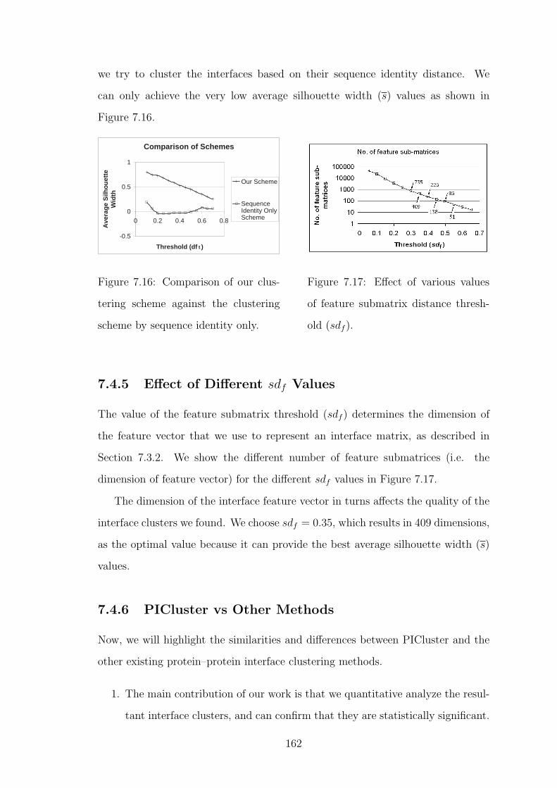
we try to cluster the interfaces based on their sequence identity distance. We

can only achieve the very low average silhouette width (s) values as shown in

Figure 7.16.

Comparison of Schemes

-0.5

0

0.5

1

0 0.2 0.4 0.6 0.8

Threshold (df t )

Ave

rag

e S

ilho

uet

te

Wid

th

Our Scheme

SequenceIdentity OnlyScheme

Figure 7.16: Comparison of our clus-

tering scheme against the clustering

scheme by sequence identity only.

Figure 7.17: Effect of various values

of feature submatrix distance thresh-

old (sdf ).

7.4.5 Effect of Different sdf Values

The value of the feature submatrix threshold (sdf ) determines the dimension of

the feature vector that we use to represent an interface matrix, as described in

Section 7.3.2. We show the different number of feature submatrices (i.e. the

dimension of feature vector) for the different sdf values in Figure 7.17.

The dimension of the interface feature vector in turns affects the quality of the

interface clusters we found. We choose sdf = 0.35, which results in 409 dimensions,

as the optimal value because it can provide the best average silhouette width (s)

values.

7.4.6 PICluster vs Other Methods

Now, we will highlight the similarities and differences between PICluster and the

other existing protein–protein interface clustering methods.

1. The main contribution of our work is that we quantitative analyze the resul-

tant interface clusters, and can confirm that they are statistically significant.

162

According to [HKK05], such an analysis and confirmation is highly desirable

for all biological data clustering systems (including interface clustering). To

our knowledge, none of the existing interface clustering method report the

statistical significance of its clusters.

2. In PICluster, we only use the pure geometrical properties (based on distance

measures) of interfaces — as opposed to using other physco-chemical prop-

erties such as hydrophobicity, packing, hydrogen bonds, and disulfide bonds.

PICluster is similar to [KTWN04, TLWN96], and different from [DS05, LCCJ99,

MSPWN05, SPMNW04] in this respect.

In our opinion, the geometrical shape is the most important factor in inferring

the functions of proteins. In other words, “function follows form” [Ros96].

Although there is no doubt that these physco-chemical properties are the

driving forces in determining the final 3D shapes of the interfaces (and more

generally the entire structures) of proteins, we believe they may be of little

use in further determining their structural similarities, and deducing their

functions. (A similar observation can be made in the field of ordinary pro-

tein structure comparison. The mainstream methods such as DALI [HS93],

CE [SB98], VAST [GMB96], and SSAP [TO89] focus only on the pure geo-

metrical properties, such as distance and angles, of protein structures rather

than their physico-chemical properties. Although there are some meth-

ods that incorporate physico-chemical properties into structural compari-

son [LMPP04, SKK98, OAA03], this approach is not widely adopted.)

3. We analyze the two interacting protein fragments on an interface simultane-

ously and synchronously (by using interface matrix representation), rather

than analyzing them separately. For this aspect, PICluster is similar to the

methods like [DS05, MSPWN05, SPMNW04], but dissimilar to [KTWN04,

SPNW04, TLWN96].

4. Since we use an easy-to-handle multi-dimensional vector representation of

the interfaces, we can compare a considerable number of interfaces in all-

163

against-all fashion within a relatively short time, as opposed to the structural

alignment-based methods which may take a tremendously long time for such

an all-against-all comparison. PICluster shares the same characteristics with

[DS05, MW03] with respect to this feature, unlike [SPMNW04, TLWN96].

Anyhow, we cannot directly compare our proposed PICluster method against

the existing interface clustering methods because their source codes or software

are not public available. Although their resultant sets of clusters are published

online, these cannot be analyzed statistically because the interface–interface simi-

larity values are not reported. Moreover, in this area of protein–protein interface

studies, there is no widely accepted standard benchmark (like SCOP and CATH in

protein classification area) to compare the performances of the different methods

objectively.

7.5 Conclusion

In this chapter we have presented a scheme for representing and clustering a rela-

tively large number of protein–protein interfaces of the protein complexes. We have

discovered quite a number of interface clusters which are biologically significant.

Firstly, we have found a number of very similar interface structures belonging to

the protein complexes from different structural fold types. This indicates the full

or partial functional similarities among diverse protein complexes. Secondly, we

have found the highly conserved motifs of well-known biological functions in some

of the interface clusters. We hope our discovery can somehow contribute useful

knowledge to real-life applications such as drug design.

164

CHAPTER 8

Conclusion and Future Work

8.1 Conclusion

Computational studies of 3D protein structures plays an important role in bioin-

formatics. In this thesis, we have presented the four methods to accomplish the

four different, yet somewhat related, tasks in the area of protein structure studies,

viz, structural alignment, database search, classification and clustering.

For protein structure alignment, we have come up with a method for detailed

structural alignment based on aligning the distance profiles. Our experimental

results show that, in a majority of cases, our method can offer better alternative

alignments to those of the commonly used methods. In particular, we can find the

tighter albeit slightly shorter alignments, which means that our method can detect

the conserved cores.

For rapid searching on large structural databases, we have proposed the use

of indexing and information retrieval (IR) strategies. The experimental results

confirm that our approach is both efficient and effective. Our system can be ideally

used as a filtering tool before a more detailed alignment process.

For protein structure classification, we have developed a nearest-neighbor clas-

sification system incorporated with active learning. We have highlighted that the

165

classification problem is different from the ordinary structural comparison and

database searching problems, and should be treated differently. Our experimental

results show that our filter-and-refine, abstract representation, and coarse scoring

schemes are well-suited for our classification purpose.

For clustering of protein–protein interfaces, we have proposed an easy-to-handle

feature vector representation based on the sub-structures of interfaces. We have

confirmed the reliability of the resultant clusters by statistical validation and visual

inspection. We have also demonstrated the usefulness of the clusters by a biological

analysis in which we can rediscover some well-known biological motifs from the

clusters.

8.2 Future Work

In this section, we discuss the possible improvements in the performances and

usability of the methods reported in the previous chapters. We also outline some

related problems that we might try to solve as our future research directions.

In order to improve the run time efficiency of the MatAlign method proposed

in Chapter 4, we plan to implement it as a parallel system. Because of its simple

nature, MatAlign is easy to be parallelized. Since most of its running time is

incurred in all-against-all alignments of the distance profiles (rows) in distance

matrices, we can assign these independent row–row alignment tasks to a number

of processors, and execute them concurrently. We also plan to test MatAlign on

a larger data set, and tune its various parameters (cell–cell distance thresholds,

bandwidth, cutoff distance for row reduction, etc.) in order to ensure a generally

good performance for any arbitrary pair of protein structures.

As for the ProtDex2 method reported in Chapter 5, we plan to work on the

updating of the inverted index after the new protein structures are added. The

current system does not support such an update, and requires to rebuild the index

when the new structures are added in batches.

For the ProtClass method presented in Chapter 6, we have a plan to assess the

166

general behavior of our scheme by trying it with a greater number of training and

testing proteins taken from a larger number of structural classes, and fine-tune the

required parameters accordingly. We also would like to look for the better strategies

for PA representation, CPset representation, and filtration so as to further improve

the system’s speed as well as its accuracy.

To further improve the usability of PICluster and its resultant clusters (Chap-

ter 7), we plan to perform some more biological data analyses on the clusters in

addition to the ones reported in this thesis. For example, we might study the

entropies of the parent protein complexes’ EC (Enzyme Commission) numbers

and GO (Gene Ontology) annotations. We will also try to carry out the clus-

tering of interfaces based on the detailed interface–interface alignment method

using a modified version of MatAlign in a distributed computing environment (as

in [MSPWN05]). We hope we can achieve better clustering results by doing so.

In addition to upgrading the existing methods, we have a plan to extend our

research into the other related areas in structural bioinformatics. It is possible

to solve the protein threading (sequence–structure alignment) problem by using

our pairwise structural alignment algorithm as a basic component. We also plan

to use some portions of both of our structural alignment and structural database

search algorithms in developing a method for homology modeling (predicting the

3D structure of a protein from its AA sequence and the 3D structures of its se-

quence homologs) and model validation (checking the resultant model). Finally, we

hope to utilize all of our expertise and knowledge in the various areas of structural

bioinformatics with a view to developing a method for ab initio structural predic-

tion (predicting a 3D protein structure directly from its AA sequence without an

additional input), which is one of the most important problems remaining unsolved

in the field of bioinformatics.

Furthermore, we ultimately plan to incorporate our methodologies in protein

structure analysis into a larger bioinformatics consortium enabling a joint learning

from multiple types of genomic data: sequences, structures, micro-arrays, protein–

protein interaction networks, metabolic pathways, etc. From such a joint explo-

167

ration system, we hope to acquire a comprehensive knowledge on the functioning

of life, and exploit this knowledge in intelligent drug design, bioengineering, food

engineering, etc., to being about the benefits for mankind.

168

BIBLIOGRAPHY

[ABC+97] R. A. Abagyan, S. Batalov, T. Cardozo, M. Totrov, and Y. Zhou.

Homology modeling with ICM: deformation zone mapping and im-

provements of models via conformational search. Proteins: Struc-

ture, Function, and Genetics, Suppl. 1:29–37, 1997.

http://www.molsoft.com/icm_browser.html.

[AF96] N. N. Alexandrov and D. Fischer. Analysis of topological and

nontopological structural similarities in the PDB: new examples

with old structures. Proteins: Structure, Function, and Genetics,

25(3):354–365, 1996.

[AFT03] Z. Aung, W. Fu, and K. L. Tan. An efficient index-based protein

structure database searching method. In Proceedings of 8th Inter-

national Conference on Database System for Advanced Applications

(DASFAA’03), pages 311–318, 2003.

[AGK05] A. S. Aytuna, A. Gursoy, and O. Keskin. Prediction of protein–

protein interactions by combining structure and sequence conserva-

tion in protein interfaces. Bioinformatics, 21(12):2850–2855, 2005.

[AGM+90] S. F. Altschul, W. Gish, W. Miller, E. W. Meyers, and D. J. Lipman.

Basic local alignment search tool. Journal of Molecular Biology,

169

215(3):403–410, 1990.

[AHB87] K. Arun, T. Huang, and S. Blostein. Least-squares fitting of two 3-

D point sets. IEEE Transactions on Pattern Analysis and Machine

Intelligence, 9(5):698–700, 1987.

[AKKS99] M. Ankerst, G. Kastenmuller, H. P. Kriegel, and T. Seidl. 3D

shape histograms for similarity search and classification in spatial

databases. In Proceedings of 6th International Symposium on Spatial

Databases (SSD’99), pages 207–226, 1999.

[Aku95] T. Akutsu. Protein structure alignment using a graph match-

ing technique. In Proceedings of Genome Informatics Workshop

(GIW’95), pages 1–8, 1995.

[AS03] N. Alexandrov and I. Shindyalov. PDP: protein domain parser.

Bioinformatics, 19(3):429–30, 2003.

[AT04a] Z. Aung and K. L. Tan. Automatic protein structure classifica-

tion through structural fingerprinting. In Proceedings of 4th IEEE

Symposium on Bioinformatics and Bioengineering (BIBE’04), pages

508–515, 2004.

[AT04b] Z. Aung and K. L. Tan. Rapid 3D protein structure database

searching using information retrieval techniques. Bioinformatics,

20(7):1045–1052, 2004.

[AT05] Z. Aung and K. L. Tan. Automatic 3D protein structure classi-

fication without structural alignment. Journal of Computational

Biology, 12(9):1221–1241, 2005.

[AT06] Z. Aung and K. L. Tan. MatAlign: precise protein structure com-

parison by matrix alignment. Journal of Bioinformatics and Com-

putational Biology, 4:1197–1216, 2006.

170

[ATNT08] Z. Aung, S. H. Tan, S. K. Ng, and K. L. Tan. PPiClust: efficient

clustering of 3-d protein-protein interaction interfaces. Journal of

Bioinformatics and Computational Biology, 6:415–433, 2008.

[BAW+05] A. Bairoch, R. Apweiler, C. H. Wu, et al. The universal protein

resource (UniProt). Nucleic Acids Research, 33:D154–159, 2005.

[BCHM96] S. E. Brenner, C. Chothia, T. J. P. Hubbard, and A. G. Murzin. Un-

derstanding protein structure: using SCOP for fold interpretation.

In Methods in Enzymology, volume 266, pages 635–643. Academic

Press, 1996.

[BDH+03] D. Bolser, P. Dafas, R. Harrington, J. Park, and M. Schroeder.

Visualisation and graph-theoretic analysis of a large-scale protein

structural interactome. BMC Bioinfromatics, 4(45), 2003.

[BFNW93] O. Bachar, D. Fischer, R. Nussinov, and H. J. Wolfson. A computer

vision based technique for 3-D sequence independent structural com-

parison of proteins. Protein Engineering, 6(3):279–288, 1993.

[BKB02] P. Bradley, P. S. Kim, and B. Berger. TRILOGY: Discovery of

sequence–structure patterns across diverse proteins. Proceedings of

the National Academy of Sciences of the United States of America,

99(13):8500–8505, 2002.

[BKL00] S. E. Brenner, P. Koehl, and M. Levitt. The ASTRAL compendium

for sequence and structure analysis. Nucleic Acids Research, 28:254–

256, 2000.

[BM03] H. Bian and L. Mazlack. Fuzzy-rough nearest-neighbor classifi-

cation approach. In Proceedings of 22nd International Confer-

ence of the North American Fuzzy Information Processing Society

(NAFIPS’03), pages 500–505, 2003.

171

[BOSD+97] E. Bertino, B. C. Ooi, R. Sacks-Davis, K. L. Tan, J. Zobel,

B. Shidlovsky, and B. Catania. Indexing Techniques for Advanced

Database Systems. Kluwer Academic Publishers, 1997.

[Bou05] P. E. Bourne. Reductionism and classification require detailed com-

parison. Biological Data Representation and Analysis lecture notes,

San Diego Supercomputer Center, 2005.

http://www.sdsc.edu/pb/edu/pharm201/12/12.ppt.

[Bre01] S. E. Brenner. A tour of structural genomics. Nature Reviews Ge-

netics, 2(10):801–809, 2001.

[BSV04] D. L. Bostick, M. Shen, and I. I. Vaisman. A simple topological

representation of protein structure: implications for new, fast, and

robust structural classification. Proteins: Structure, Function, and

Bioinformatics, 56(3):487–501, 2004.

[BT98] A. A. Bogan and K. S. Thorn. Anatomy of hot spots in protein

interfaces. Journal of Molecular Biology, 280(1):1–9, 1998.

[BT99] C. Branden and J. Tooze. Introduction to Protein Structure. Garland

Publishing, 2nd edition, 1999.

[BWF+00] H. M. Berman, J. Westbrook, Z. Feng, G. Gilliland, T.N. Bhat,

H. Weissig, I.N. Shindyalov, and P.E. Bourne. The protein data

bank. Nucleic Acids Research, 28:235–242, 2000.

[BYRN99] R. Baeza-Yates and B. Ribeiro-Neto. Modern Information Retrieval.

ACM Press, 1999.

[CCI+04] A. Caprara, R. Carr, S. Istrail, G. Lancia, and B. Walenz. 1001

optimal PDB structure alignments: integer programming methods

for finding the maximum contact map overlap. Journal of Compu-

tational Biology, 11(1):27–52, 2004.

172

[CCSW05] O. Camoglu, T. Can, A. K. Singh, and Y. F. Wang. Decision tree

based information integration for automated protein classification.

Journal of Bioinformatics and Computational Biology, 3(3):717–

742, 2005.

[CGZ04] M. Comin, C. Guerra, and G. Zanotti. PROuST: a server-based

comparison method of three-dimensional structures of proteins using

indexing techniques. Journal of Computational Biology, 11(6):1061–

1072, 2004.

[CH88] G. M. Crippen and T. F. Havel. Distance Geometry and Molecular

Conformation. John Wiley and Sons, 1988.

[CHTY05] C. H. Chionh, Z. Huang, K. L. Tan, and Z. Yao. Towards scaleable

protein structure comparison and database search. International

Journal on Artificial Intelligence Tools, 14(5):827–848, 2005.

[CJ02] P. Chakrabarti and J. Janin. Dissecting protein–protein recognition

sites. Proteins: Structure, Function and Genetics, 47(3):334–343,

2002.

[CKK04] I. G. Choi, J. Kwon, and S. H. Kim. Local feature frequency profile:

a method to measure structural similarity in proteins. Proceedings of

the National Academy of Sciences of the United States of America,

101(11):3797–3802, 2004.

[CKS04] O. Camoglu, T. Kahveci, and A. K. Singh. Index-based similarity

search for protein structure databases. Journal of Bioinformatics

and Computational Biology, 2(1):99–126, 2004.

[CP02] O. Carugo and S. Pongor. Protein fold similarity estimated by a

probabilistic approach based on C(alpha)–C(alpha) distance com-

parison. Journal of Molecular Biology, 315(4):887–898, 2002.

173

[CSM04] A. Chinnasamy, W. K. Sung, and A. Mittal. Protein structure and

fold prediction using tree-augmented bayesian classifier. In Proceed-

ings of 9th Pacific Symposium on Biocomputing (PSB’04), pages

387–398, 2004.

[DBG+03] P. Dafas, D. Bolser, J. Gomoluch, J. Park, and M. Schroeder.

Fast and efficient computation of domain–domain interactions from

known protein structures in the PDB. In Proceedings of German

Conference Bioinformatics on 2003 (GCB’03), pages 27–32, 2003.

[DD01] C. H. Q. Ding and I. Dubchak. Multi-class protein fold recognition

using support vector machines and neural networks. Bioinformatics,

17:349–358, 2001.

[DFGB+03] P. Dombrosky-Ferlan, A. Grishin, R. J. Botelho, M. Sampson,

L. Wang, W. A. Rudert, S. Grinstein, and S. J. Corey. Felic (CIP4b),

a novel binding partner with the Src kinase Lyn and Cdc42, localizes

to the phagocytic cup. Blood, 101(7):2804–2809, 2003.

[dHINM04] M. J. L. de Hoon, S. Imoto, J. Nolan, and S. Miyano. Open source

clustering software. Bioinformatics, 20(9):1453–1454, 2004.

[DS05] F. P. Davis and A. Sali. PIBASE: a comprehensive database of

structurally defined protein interfaces. Bioinformatics, 21(9):1901–

1907, 2005.

[Dun03] M. H. Dunham. Data Mining: Introductory and Advanced Topics.

Prentice Hall, 2003.

[DWNT99] D. Gilbert D, D. Westhead, N. Nagano, and J. Thornton. Motif-

based searching in tops protein topology databases. Bioinformatics,

15(4):317–326, 1999.

174

[EA62] C. J. Epstein and C. B. Anfinsen. The reversible reduction of disul-

fide bonds in Trypsin and Ribonuclease coupled to Carboxymethyl

Cellulose. Journal of Biological Chemistry, 237:2175–2179, 1962.

[EJT00] I. Eidhammer, I. Jonassen, and W. R. Taylor. Protein structure

comparison and structure patterns. Journal of Computational Biol-

ogy, 7(5):685–716, 2000.

[Erd05] M. A. Erdmann. Protein similarity from knot theory: geometric

convolution and line weavings. Journal of Computational Biology,

12(6):609–637, 2005.

[FA95] D. Frishman and P. Argos. Knowledge-based secondary structure

assignment. Proteins: Structure, Function and Genetics, 23:566–

579, 1995.

[FC96] A. Falicov and F. E. Cohen. A surface of minimum area metric for

the structural comparison of proteins. Journal of Molecular Biology,

258(5):871–892, 1996.

[FERE96] D. Fischer, A. Elofsson, D. Rice, and D. Eisenberg. Assessing the

performance of fold recognition methods by means of a compre-

hensive benchmark. In Proceedings of 1996 Pacific Symposium on

Biocomputing (PSB’96), pages 300–318, 1996.

[FPVC02] P. Fariselli, F. Pazos, A. Valencia, and R. Casadio. Prediction of

protein–protein interaction sites in heterocomplexes with neural net-

works. European Journal of Biochemistry, 269(5):1356–1361, 2002.

[FS96] Z. K. Feng and M. J. Sippl. Optimum superimposition of protein

structures: ambiguities and implications. Fold and Design, 1(2):123–

132, 1996.

175

[FTNW95] D. Fischer, C. J. Tsai, R. Nussinov, and H. J. Wolfson. A 3D

sequence-independent representation of the protein data bank. Pro-

tein Engineering, 8:981–997, 1995.

[GARW93] H. Grindley, P. Artymiuk, D. Rice, and P. Willett. Identification of

tertiary structure resemblance in proteins using a maximal common

sub-graph isomorphism algorithm. Journal of Molecular Biology,

229:707–721, 1993.

[GFH03] S. Goldsmith-Fischman and B. Honig. Structural genomics: compu-

tational methods for structure analysis. Protein Science, 12:1813–

1821, 2003.

[GL96] M. Gerstein and M. Levitt. Using iterative dynamic programming to

obtain accurate pairwise and multiple alignments of protein struc-

tures. In Proceedings of 4th International Conference on Intelligent

Systems for Molecular Biology (ISMB’96), pages 59–67, 1996.

[GMB96] J. F. Gibrat, T. Madej, and H. Bryant. Surprising similarities in

structure comparison. Current Opinion in Structural Biology, 6:377–

385, 1996.

[God96] A. Godzik. The structural alignment between two proteins: is there

a unique answer? Protein Science, 5(7):1325–1338, 1996.

[GRSE99] J. Grassmann, M. Reczko, S. Suhai, and L. Edler. Protein fold class

prediction: new methods of statistical classification. In Proceedings

of 7th International Conference on Intelligent Systems for Molecular

Biology (ISMB’99), pages 106–112, 1999.

[GSLB99] J. Gorodkin, H. H. Stærfeldt, O. Lund, and S. Brunak. MatrixPlot:

visualizing sequence constraints. Bioinformatics, 15:769–770, 1999.

http://www.cbs.dtu.dk/services/MatrixPlot/.

176

[GZ05] F. Gao and M. J. Zaki. PSIST: Indexing protein structures using

suffix trees. In Proceedings of IEEE Computational Systems Bioin-

formatics Conference (CSB’05), pages 212–222, 2005.

[HAB+97] T. J. P. Hubbard, B. Ailey, S. E. Brenner, A. G. Murzin, and

C. Chothia. SCOP: a structural classification of proteins database.

Nucleic Acids Research, 25(1):236–239, 1997.

[HBW+05] J. Huan, D. Bandyopadhyay, W. Wang, J. Snoeyink, J. Prins, and

A. Tropsha. Comparing graph representations of protein structure

for mining family-specific residue-based packing motifs. Journal of

Computational Biology, 12(6):657–671, 2005.

[HK05] J. Han and M. Kamber. Data Mining: Concepts and Techniques.

Morgan Kaufmann Publishers, 2nd edition, 2005.

[HKK05] J. Handl, J. Knowles, and D. B. Kell. Computational cluster vali-

dation in post-genomic data analysis. Bioinformatics, 21(15):3201–

3212, 2005.

[HMWN00] Z. Hu, B. Ma, H. Wolfson, and R. Nussinov. Conservation of polar

residues as hot spots at protein interfaces. Proteins: Structure,

Function and Genetics, 39(4):331–342, 2000.

[HP00] L. Holm and J. Park. DaliLite workbench for protein structure

comparison. Bioinformatics, 16(6):566–567, 2000.

[HPS+03] A. Harrison, F. Pearl, I. Sillitoe, T. Slidel, R. Mott, J. Thornton,

and C. Orengo. Recognizing the fold of a protein structure. Bioin-

formatics, 19(14):1748–59, 2003.

[HS93] L. Holm and C. Sander. Protein structure comparison by alignment

of distance matrices. Journal of Molecular Biology, 233:123–138,

1993.

177

[HS94a] L. Holm and C. Sander. The FSSP database of structurally aligned

protein fold families. Nucleic Acids Research, 22(17):3600–3609,

1994.

[HS94b] L. Holm and C. Sander. Parser for protein folding units. Proteins:

Structure, Function and Genetics, 19:256–268, 1994.

[HS94c] L. Holm and C. Sander. Searching protein structure databases has

come of age. Proteins: Structure, Function and Genetics, 19:165–

173, 1994.

[HS95] L. Holm and C. Sander. 3-D lookup: fast protein structure database

searches at 90% reliability. In Proceedings of 3rd International Con-

ference on Intelligent Systems for Molecular Biology (ISMB’95),

pages 179–187, 1995.

[HS98] L. Holm and C. Sander. Dictionary of recurrent domains in protein

structures. Proteins: Structure, Function and Genetics, 33:88–96,

1998.

[HSZK03] J. Hou, G. E. Sims, C. Zhang, and S. H. Kim. A global representa-

tion of the protein fold space. Proceedings of the National Academy

of Sciences of the United States of America, 100(3):2386–2390, 2003.

[HWW+04] J. Huan, W. Wang, A. Washington, J. Prins, and A. Tropsha. Accu-

rate classification of protein structural families using coherent sub-

graph analysis. In Proceedings of 9th Pacific Symposium on Bio-

computing (PSB’04), pages 411–422, 2004.

[HZS05] Z. H. Huang, X. Zhou, and D. Song. High dimensional indexing

for protein structure matching using Bowties. In Proceedings of 3rd

Asia-Pacific Bioinformatics Conference (APBC’05), pages 21–30,

2005.

178

[IYS04] Z. Isik, B. Yanikoglu, and U. Sezerman. Protein structural class

determination using support vector machines. In Proceedings of 19th

International Symposium on Computer and Information Sciences

(ISCIS’04), pages 82–89, 2004.

[JECT02] I. Jonassen, I. Eidhammer, D. Conklin, and W. R. Taylor. Structure

motif discovery and mining the PDB. Bioinformatics, 18:362–367,

2002.

[Kab78] W. Kabsch. A discussion of the solution for the best rotation to re-

late two sets of vectors. Acta Crystallographica Section A, A34:827–

828, 1978.

[Kar03] Kevin Karplus, University of California Santa Cruz. Personal com-

munications, September 2003.

[KFDDG02] M. Kirsten Frank, F. Dyda, A. Dobrodumov, and A. M. Gronen-

born. Core mutations switch monomeric protein GB1 into an inter-

twined tetramer. Nature Structural Biology, 9(11):877–885, 2002.

[KGME02] G. Kleiger, R. Grothe, P. Mallick, and D. Eisenberg. GXXXG and

AXXXA: common alpha-helical interaction motifs in proteins, par-

ticularly in extremophiles. Biochemistry, 41(19):5990–5997, 2002.

[KH04] E. Krissinel and K. Henrick. Secondary-structure matching (SSM),

a new tool for fast protein structure alignment in three dimensions.

Acta Crystallographica Section D, D60:2256–2268, 2004.

[Kim94] J. W. Kimball. Biology. Wm. C. Brown Publishers, 6th edition,

1994.

[KJ94] G. J. Kleywegt and A. Jones. Superposition. CCP4/ESF-EACBM

Newsletter on Protein Crystallography, 31:9–14, 1994.

179

[KJ97] G.J. Kleywegt and T. A. Jones. Detecting folding motifs and sim-

ilarities in protein structures. In Methods in Enzymology, volume

277, pages 525–545. Academic Press, 1997.

[KKL05] R. Kolodny, P. Koehl, and M. Levitt. Comprehensive evaluation

of protein structure alignment methods: scoring by geometric mea-

sures. Journal of Molecular Biology, 346:1173–1188, 2005.

[KL97] I. Koch and T. Lengauer. Detection of distant structural similarities

in a set of proteins using a fast graph-based method. In Proceedings

of 5th International Conference on Intelligent Systems for Molecular

Biology (ISMB’97), pages 167–187, 1997.

[Kle96] G.J. Kleywegt. Use of non-crystallographic symmetry in protein

structure refinement. Acta Crystallographica Section D, D52:842–

857, 1996.

[KN00] T. Kawabata and K. Nishikawa. Protein structure comparison us-

ing the Markov transition model of evolution. Proteins: Structure,

Function, and Genetics, 41:108–122, 2000.

[Koe01] P. Koehl. Protein structure similarities. Current Opinion in Struc-

tural Biology, 11:348–353, 2001.

[KR90] L. Kaufman and P. J. Rousseeuw. Finding Groups in Data: An

Introduction to Cluster Analysis. Wiley-Interscience, 1990.

[KS83] W. Kabsch and C. Sander. DSSP: definition of secondary structure

of proteins given a set of 3D coordinates. Biopolymers, 22:2577–

2637, 1983.

[KTWN04] O. Keskin, C. J. Tsai, H. Wolfson, and R. Nussinov. A new, struc-

turally nonredundant, diverse data set of protein–protein interfaces

and its implications. Protein Science, 13:1043–1055, 2004.

180

[LCCJ99] L. Lo Conte, C. Chothia, and J. Janin. The atomic structure of

protein–protein recognition sites. Journal of Molecular Biology,

285(5):2177–2198, 1999.

[LFNW01] N. Leibowitz, Z. Fligelman, R. Nussinov, and H. J. Wolfson. Au-

tomated multiple structure alignment and detection of a common

substructural motif. Proteins: Structure, Function, and Genetics,

43:235–245, 2001.

[LG98] M. Levitt and M. Gerstein. A unified statistical framework for se-

quence comparison and structure comparison. Proceedings of the

National Academy of Sciences of the United States of America,

95(11):5913–5920, 1998.

[LI03] G. Lancia and S. Istrail. Protein structure comparison: algorithms

and applications. In C. Guerra and S. Istrail, editors, Mathemati-

cal Methods for Protein Structure Analysis and Design, pages 1–33.

Springer-Verlag Heidelberg, 2003.

[Lic01] O. Lichtarge. Getting past appearances: the many-fold conse-

quences of remote homology. Nature Structural Biology, 8:918–920,

2001.

[LLTN04] H. Li, J. Li, S.H. Tan, and S. K. Ng. Discovery of binding motif

pairs from protein complex structural data and protein interaction

sequence data. In Proceedings of 9th Pacific Symposium on Biocom-

puting (PSB’04), pages 312–323, 2004.

[LMPP04] H. Li, K. Marsolo, S. Parthasarathy, and Dmitrii Polshakov. A new

approach to protein structure mining and alignment. In Proceedings

of 4th ACM SIGKDD Workshop on Data Mining in Bioinformatics

(BIOKDD’04), 2004.

181

[Mar00] A. C. R. Martin. The ups and downs of protein topology: rapid

comparison of protein structure. Protein Engineering, 13:829–837,

2000.

[MEWN03] B. Ma, T. Elkayam, H. Wolfson, and R. Nussinov. Protein–protein

interactions: structurally conserved residues distinguish between

binding sites and exposed protein surfaces. Proceedings of the

National Academy of Sciences of the United States of America,

100(10):5772–5777, 2003.

[MH87] F. Murtagh and A. Heck. Multivariate Data Analysis. Kluwer Aca-

demic Publishers, 1987.

[MLM+05] J. Martin, G. Letellier, A. Marin, J. F. Taly, A. G. de Brevern, and

J. F. Gibrat. Protein secondary structure assignment revisited: a

detailed analysis of different assignment methods. BMC Structural

Biology, 5(17), 2005.

[MSMP99] H. Muller, D. M. Squire, W. Muller, and T. Pun. Efficient access

methods for content-based image retrieval with inverted files. In Pro-

ceedings of Multimedia Storage and Archiving Systems IV (VV’02),

1999.

[MSPWN05] S. Mintz, A. Shulman-Peleg, H. J. Wolfson, and R. Nussinov. Gener-

ation and analysis of a protein–protein interface data set with similar

chemical and spatial patterns of interactions. Proteins: Structure,

Function, and Bioinformatics, 61:6–20, 2005.

[MW03] J. Mintseris and Z. Weng. Atomic contact vectors in protein–protein

recognition. Proteins: Structure, Function, and Genetics, 53:629–

639, 2003.

[NMK04] M. Novotny, D. Madsen, and G. J. Kleywegt. Evaluation of protein

fold comparison servers. Proteins: Structure, Function and Bioin-

formatics, 54:260–270, 2004.

182

[NT04] S. K. Ng and S. H. Tan. Discovering protein–protein interactions.

Journal of Bioinformatics and Computational Biology, 1(4):711–

741, 2004.

[NW71] S. B. Needleman and C. D. Wunsch. A general method applicable to

the search for similarities in the amino acid sequence of two proteins.

Journal of Molecular Biology, 48:443–453, 1971.

[NW91] R. Nussinov and H. J. Wolfson. Efficient detection of three-

dimensional structural motifs in biological macromolecules by com-

puter vision techniques. Proceedings of the National Academy of

Sciences of the United States of America, 88:10495–10499, 1991.

[OAA03] S. D. O’Hearn, A.J.Kusalik, and J. F. Angel. MolCom: a method

to compare protein molecules based on 3-D structural and chemical

similarity. Protein Engineering, 16(2):169–178, 2003.

[OHN99] T. Ohkawa, S. Hirayama, and H. Nakamura. A method of compar-

ing protein structures based on matrix representation of secondary

structure pairwise topology. In Proceedings of 4th IEEE Symposium

on Intelligence in Neural and Biological Systems (INBS’99), pages

10–15, 1999.

[OJT03] C. Orengo, D. Jones, and J. Thornton. Bioinformatics: Genes,

Proteins and Computers. Oxford BIOS Scientific Press, 2003.

[OMJ+97] C. A. Orengo, A. D. Michie, S. Jones, D. T. Jones, M.B. Swindells,

and J.M. Thornton. CATH: a hierarchic classification of protein

domain structures. Structure, 5(8):1093–1108, 1997.

[Ore99] C. A. Orengo. CORA: topological fingerprints for protein structural

families. Protein Science, 8:699–715, 1999.

[OSO02] A. R. Ortiz, C. E. M. Strauss, and O. Olmea. MAMMOTH

(Matching Molecular Models Obtained from THeory): an auto-

183

mated method for protein model comparison. Protein Science,

11:2606–2621, 2002.

[PD75] E. A. Padlan and D. R. Davies. Variability of three-dimensional

structure in Immunoglobulins. Proceedings of the National Academy

of Sciences of the United States of America, 72(3):819–823, 1975.

[PEB+04] U. Pieper, N. Eswar, H. Braberg, et al. MODBASE, a database

of annotated comparative protein structure models, and associated

resources. Nucleic Acids Research, 32:D217–222, 2004.

[PL04] J. Przyborski and M. Lanzer. Parasitology. The malarial secretome.

Science, 306(5703):1897–1898, 2004.

[PLG+03] P. Puntervoll, R. Linding, C. Gemund, et al. ELM server: A new re-

source for investigating short functional sites in modular eukaryotic

proteins. Nucleic Acids Research, 31(13):3625–3630, 2003.

[PLT01] J. Park, M. Lappe, and S. A. Teichmann. Mapping protein fam-

ily interactions: intramolecular and intermolecular protein family

interaction repertoires in the PDBand yeast. Journal of Molecular

Biology, 307(3):929–938, 2001.

[PR04a] S. H. Park and K. H. Ryu. Effective filtering for structural similar-

ity search in protein 3D structure databases. In Proceedings of 15th

International Conference on Database and Expert Systems Applica-

tions (DEXA’04), pages 761–770, 2004.

[PR04b] S. H. Park and K. H. Ryu. Fast similarity search for protein 3D

structure databases using spatial topological patterns. In Proceed-

ings of 15th International Conference on Database and Expert Sys-

tems Applications (DEXA’04), pages 771–780, 2004.

[RA76] M. G. Rossmann and P. Argos. Exploring structural homology of

proteins. Journal of Molecular Biology, 105:75–95, 1976.

184

[RA00] J. Rosamond and A. Allsop. Harnessing the power of the genome in

the search for new antibiotics. Science, 287(5460):1973–1976, 2000.

[RCGRA+04] B. Ravi Chandra, R. Gowthaman, R. Raj Akhouri, D. Gupta, and

A. Sharma. Distribution of proline-rich (PxxP) motifs in distinct

proteomes: functional and therapeutic implications for malaria and

tuberculosis. Protein Engineering Design and Selection, 17(2):175–

182, 2004.

[RE00] W. P. Russ and D. M. Engelman. The GxxxG motif: a framework

for transmembrane helix-helix association. Journal of Molecular Bi-

ology, 296(3):911–919, 2000.

[RF03] P. Røgen and B. Fain. Automatic classification of protein structure

by using Gauss integrals. Proceedings of the National Academy of

Sciences of the United States of America, 100(1):119–124, 2003.

[RG88] S. Rackovsky and D. A. Goldstein. Protein comparison and classi-

fication: a differential geometric approach. Proceedings of the Na-

tional Academy of Sciences of the United States of America, 85:777–

781, 1988.

[Ros96] G. D. Rose. No assembly required. The Sciences, 36:26–31, 1996.

[Ros99] B. Rost. Twilight zone of protein sequence alignments. Protein

Engineering, 12(2):85–94, 1999.

[Ros03] B. Rost. Predict structure and function: biochemistry and molecular

biology of eukaryotes. Bioinformatics 2003 lecture notes, CUBIC

Columbia University, 2003. http://cubic.bioc.columbia.edu/

talks/course-2003/cu2/cu2.ppt.

[SB90] A. Sali and T. L. Blundell. Definition of general topological equiv-

alence in protein structures: a procedure involving comparison of

185

properties and relationships through simulated annealing and dy-

namic programming. Journal of Molecular Biology, 212:403–428,

1990.

[SB97] A. P. Singh and D. L. Brutlag. Hierarchical protein structure su-

perposition using both secondary structure and atomic representa-

tions. In Proceedings of 5th International Conference on Intelligent

Systems for Molecular Biology (ISMB’97), pages 284–293, 1997.

[SB98] I. N. Shindyalov and P. E. Bourne. Protein structure alignment

by incremental combinatorial extension (CE) of the optimal path.

Protein Engineering, 11(9):739–747, 1998.

[SCSX04] C. R. Shyu, P. H. Chi, G. Scott, and D. Xu. ProteinDBS — a

content-based retrieval system for protein structure database. Nu-

cleic Acids Research, 32:w572–575, 2004.

[Sfy04] K. Sfyrakis. Geometrical transformations, 2004.

http://lcvmwww.epfl.ch/~kostas/GeometricalTransformations.

htm#Anchor-New-49572.

[SH03] E. S. C. Shih and M. J. Hwang. Protein structure comparison by

probability-based matching of secondary structure elements. Bioin-

formatics, 19:735–741, 2003.

[Sha48] C. E. Shannon. A mathematical theory of communication. Bell

System Technical Journal, 27:379–423, 1948.

[SKK98] T. Seidl, G. Kastenmuller, and H. P. Kriegel. Similarity search in

3D protein databases. In Proceedings of German Conference on

Bioinformatics, 1998.

[SLL93] S. Subbiah, D. V. Laurents, and M. Levitt. Structural similarity of

DNA-binding domains of bacteriophage repressors and the globin

core. Current Biology, 3:141–148, 1993.

186

[SM97] J. C. Setubal and J. Meidanis. Introduction to Computational Biol-

ogy. PWS Publishing, 1997.

[SM01] E. Sprinzak and H. Margalit. Correlated sequence-signatures as

markers of protein–protein interaction. Journal of Molecular Biol-

ogy, 311(4):681—692, 2001.

[SP04] M. L. Sierk and W. R. Pearson. Sensitivity and selectivity in protein

structure comparison. Protein Science, 13:773–785, 2004.

[SPMNW04] A. Shulman-Peleg, S. Mintz, R. Nussinov, and H. J. Wolfson.

Protein–protein interfaces: recognition of similar spatial and chem-

ical organizations. In Proceedings of 4th International Workshop

Algorithms in Bioinformatics (WABI’04), pages 194–205, 2004.

[SPNW04] A. Shulman-Peleg, R. Nussinov, and H. J. Wolfson. Recognition of

functional sites in protein structures. Journal of Molecular Biology,

339(3):607–633, 2004.

[SSS02] B. Schmidt, H. Schorder, and M. Schimmler. Massively parallel

solutions for molecular sequence analysis. In Proceedings of 2nd

IEEE International Workshop on High Performance Computational

Biology (HiCOMB’02), page 201, 2002.

[Sun04] D. Sunday. Distance between lines and segments with their clos-

est point of approach, 2004. http://softsurfer.com/Archive/

algorithm_0106/algorithm_0106.htm.

[SW81] T. F. Smith and M. S. Waterman. Comparison of biosequences.

Advances in Applied Mathematics, 2:482–489, 1981.

[SW00] J. D. Szustakowski and Z. Weng. Protein structure alignment using

a genetic algorithm. Proteins: Structure, Function, and Genetics,

38:428–440, 2000.

187

[Tay02] W. R. Taylor. Protein structure comparison using bipartite graph

matching and its application to protein structure classification.

Molecular and Cellular Proteomics, 1:334–339, 2002.

[TLWN96] C. J. Tsai, S. L. Lin, H. J. Wolfson, and R. Nussinov. A

dataset of protein–protein interfaces generated with sequence-order-

independent comparison technique. Journal of Molecular Biology,

260:604–620, 1996.

[TO89] W. R. Taylor and C. A. Orengo. Protein structure alignment. Jour-

nal of Molecular Biology, 208:1–22, 1989.

[TSN04] S. H. Tan, W. K. Sung, and S. K. Ng. Discovering novel inter-

acting motif pairs from large protein–protein interaction datasets.

In Proceedings of 4th IEEE Symposium on Bioinformatics and Bio-

engineering (BIBE’04), pages 568–575, 2004.

[TT04] Z. Tan and A. K. H. Tung. Substructure clustering on sequential

3D object datasets. In Proceedings of 20th International Conference

on Data Engineering (ICDE’04), pages 634–645, 2004.

[TXN97] C. J. Tsai, D. Xu, and R. Nussinov. Structural motifs at protein–

protein interfaces: protein cores versus two-state and three-state

model complexes. Protein Science, 6(9):1793–1805, 1997.

[VBAS04] S. Veretnik, P. E. Bourne, N. N. Alexandrov, and I. N. Shindyalov.

Toward consistent assignment of structural domains in proteins.

Journal of Molecular Biology, 339:647–678, 2004.

[vMKS+02] C. von Mering, R. Krause, B. Snel, M. Cornell, S. G. Oliver,

S. Fields, and P. Bork. Comparative assessment of large-scale data

sets of protein–protein interactions. Nature, 417:399–403, 2002.

[WCH05] S. L. Wang, C. M. Chen, and M. J. Hwang. Classification of pro-

tein 3D folds by hidden Markov learning on sequences of structural

188

alphabets. In Proceedings of 3rd Asia-Pacific Bioinformatics Con-

ference (APBC’05), pages 65–72, 2005.

[WFB03] S. Wallin, J. Farwer, and U. Bestolla. Testing similarity measures

with continuous and discrete protein models. Proteins: Structure,

Function, and Genetics, 50(1):144–157, 2003.

[Wik06] Wikimedia, Foundation. Wikipedia: The Free Encyclopedia, 2006.

http://en.wikipedia.org/.

[WKHK04] N. Weskamp, D. Kuhn, E. Hullermeier, and G. Klebe. Efficient

similarity search in protein structure databases by k-clique hashing.

Bioinformatics, 20:1522–1526, 2004.

[Wol01] H. Wolfson. Protein structure. Algorithms in Molecular Biology

lecture notes, Tel Aviv University, 2001.

http://www.math.tau.ac.il/~rshamir/algmb/01/scribe12/

lec12.ps.gz.

[WR97] H. J. Wolfson and I. Rigoutsos. Geometric hashing: an overview.

IEEE Computational Science and Engineering, 4(4):10–21, 1997.

[WSB98] R. Weber, H. J. Schek, and S. Blott. A quantitative analysis and per-

formance study for similarity-search methods in high-dimensional

spaces. In Proceedings of 24th International Conference on Very

Large Data Bases (VLDB’98), pages 194–205, 1998.

[Wu03] Z. Wu. Protein structure determination and dynamic simula-

tion. ISU Summer Institute on Bio-Informatics lecture notes,

Iowa State University, 2003. http://www.math.iastate.edu/wu/

LectureNotes/SummerInstitute.ppt.

[WZ02] H. E. Williams and J. Zobel. Indexing and retrieval for genomic

databases. IEEE Transactions on Knowledge and Data Engineering,

14(1):63–78, 2002.

189

[YCCO05] J. S. Yeh, D. Y. Chen, B. Y. Chen, and M. Ouhyoung. A web-

based three-dimensional protein retrieval system by matching visual

similarity. Bioinformatics, 21(13):3056–3057, 2005.

[YG03] Y. Ye and A. Godzik. Flexible structure alignment by chaining

aligned fragment pairs allowing twists. Bioinformatics, 19 Suppl.

1:ii246–255, 2003.

[Yon02] G. Yona. Protein classification and meta-organization. Methods for

global organization of the protein universe. Tutorial in 10th Inter-

national Conference on Intelligent Systems for Molecular Biology

(ISMB’02), 2002.

http://www.cs.cornell.edu/golan/Papers/ismb2002.ppt.

[ZG02] B. Zhang and A. Godzik. The meaning and limitations of pro-

tein structure alignments. In Proceedings of 1st International Sym-

posium on 3D Data Processing Visualization and Transmission

(3DPVT’02), pages 729–726, 2002.

[ZIB01] J. Zachary, S. S. Iyengar, and J. Barhen. Content based image

retrieval and information theory: a general approach. Journal

of the American Society for Information Science and Technology,

52(10):840–852, 2001.

[ZK03] C. Zhang and S. H. Kim. Overview of structural genomics: from

structure to function. Current Opinion In Chemical Biology, 7:28–

32, 2003.

[ZW05] J. Zhu and Z. Weng. FAST: a novel protein structure alignment algo-

rithm. Proteins: Structure, Function, and Bioinformatics, 58:618–

627, 2005.

190

Documents

COMPUTATIONAL ANALYSIS OF 3D PROTEIN STRUCTURES · PDF fileCOMPUTATIONAL ANALYSIS OF 3D PROTEIN STRUCTURES ZEYAR AUNG National University of Singapore 2006 Note: This thesis was slightly