Embed Size (px)
Citation preview
X-541-66-196
COMPUTATION OF THE LONG RANGE MOTION OF A LUNAR SATELLITE
BY . - ,
ISABELLA J. COLE
GPO PRICE $
- CFSTI PRICE(S) f \
,dV Microfiche (MF) MAY I966
GODDARD SPACE FL16HT CENTER GREENBELT, MARYLAND
ff 853 July 65
0353 (ACCESSION NUMBER).
sN66 3
2 <
OR OR TUX OR AD NUMBER) (CATEGORY)
https://ntrs.nasa.gov/search.jsp?R=19660021063 2019-04-27T14:20:15+00:00Z
X-547-66- 196
COMPUTATION OF THE LONG RANGE MOTION
OF A LUNAR SATELLITE
bY
Isabella J. Cole
Goddard Space Flight Center Greenbelt, Maryland
I
CONTENTS
page - SUMMARY ......................................... V
LIST OF SYMBOLS. . ................................. vi
INTRODUCTION ...................................... 1
THE HARMONIC ANALYSIS METHOD ...................... 1
THE SOLUTION WITH ELLIPTIC INTEGRAIS . . . . . . . . . . . . . . . . 14
REFERENCES AND BIBLIOGRAPHY ....................... 32
iii

COMPUTATION OF THE LONG RANGE MOTION
OF A LUNAR SATELLITE
Isabella J. Cole
SUMMARY
Formulae for long periodic perturbations depending on the argument of the pericenter are derived by the method of Harmonic Analysis and with Elliptic Integrals.
An approximation of the terms of the Energy Integral that are de- pendent on the oblateness was used in the solution with Elliptic Integrals.
V

LIST OF SYMBOLS
a = semimajor axis of the satellite's orbit = L2/p.
b = mean radius of the moon (.1738 decamegametres) .
e = eccentricity of the satellite's orbit = L2
g = argument of pericenter of the satellite.
h = longitude of the ascending node of the lunar satellite.
H = G c o s i
i = inclination of the satellite's orbit plane to the moon's equatorial plane =
cos'l H/C
J, = principal part of the oblateness of the moon (2.41 X
3 4
K, = - J, b2 n2
4 = mean anomaly of the lunar satellite.
n = mean motion of the satellite = p2/L3.
nc = mean motion of the moon's mean anomaly = 2.2802713 x (radiudcentiday).
n: = mean motion of the moon's mean longitude = 2.2997150 x (radians/centiday).
vi
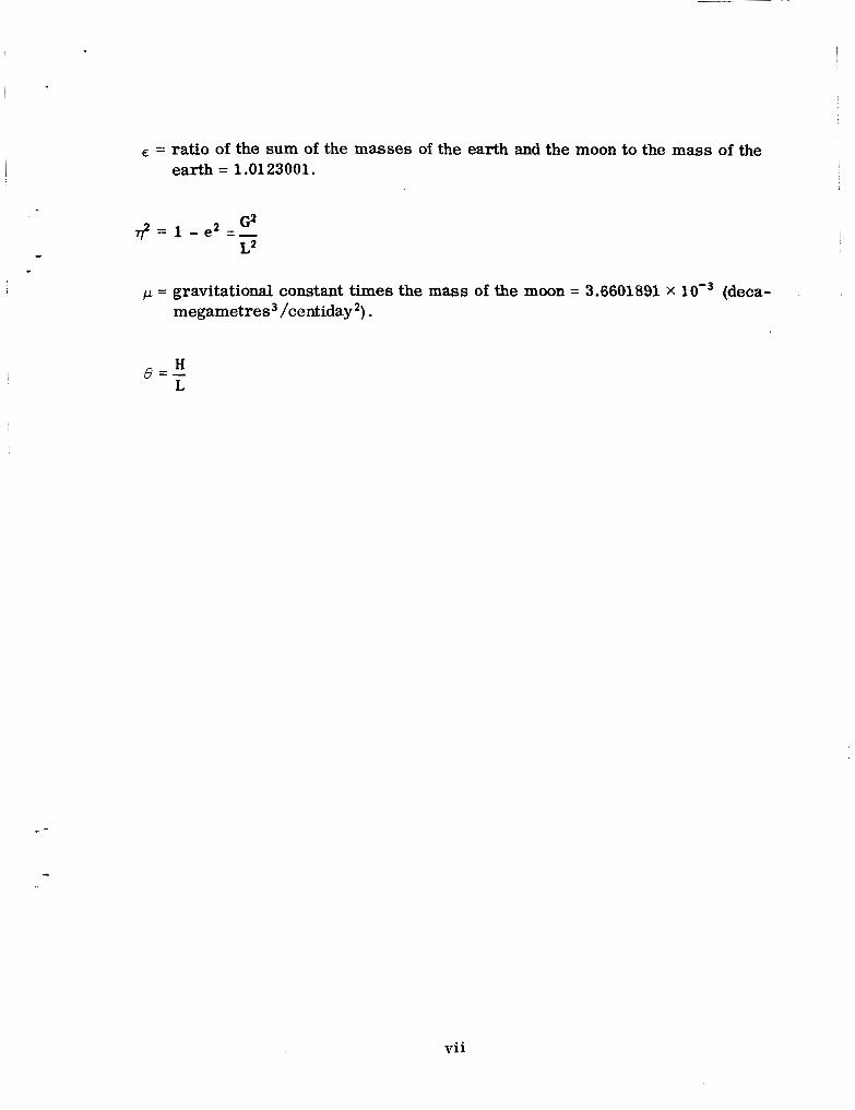
E = ratio of the sum of the masses of the earth and the moon to the mass of the earth = 1.0123001.
p = gravitational constant times the mass of the moon = 3.6601891 X (deca- megametres3 /centiday*) .
H L
&J=-
vii

COMPUTATION OF THE LONG RANGE MOTION
OF A LUNAR SATELLITE
INTRODUCTION
In this paper formulae for dt/dt, dh/dt, 4 and h that were derived by:
1. The method of Harmonic Analysis and
2. With Elliptic Integrals are presented.
To preserve the continuity of the presentation the formula for g , q2 and dg/d t from reference 1 a re also given. In the solution with Elliptic Integrals formulae for dt/d t, dh/d t and d g /d t are presented from reference 3.
THE HARMONIC ANALYSIS METHOD
The Harmonic Analysis Method is presented for the computation of the long range motion of a Lunar Satellite. The procedure, as outlined below, is well adapted to high speed digital computers and attempts to reduce the amount of labor involved in the computation.
a. Derivation of q2 as a Cosine Series
The Hamiltonian, F is given by
F = F, + F, i- F,
where
F, = n; H
1

I- .
Author's Approximation
F, = ~ K , L ( (5 - 3q2) (5- 1) ,.
Binomial Expansion E r r o r
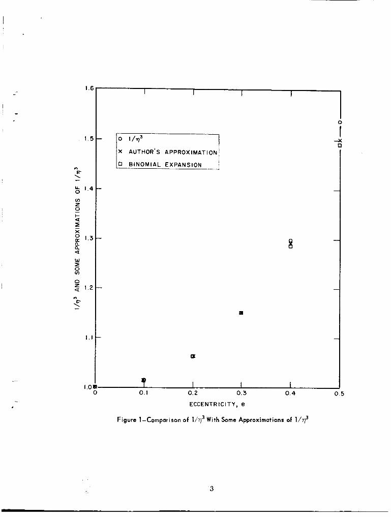
One seeks now an approximation for 1 / q 3 (dependent on the value of e ' ) so that one has a quadratic in e2. The truncated binomial expansion of l/q3 !s (1 + (3/2)e2 + (15/8)e4). However, a better approximation for 1 /q3 is ( 1 + (3/2)e2 + 2 e4 ) . The following table compares this approximation, the actual value of 1 /773 and the binomial expansion of 1 / q 3 . This approximation was derived empirically and is accurate for 0 s e I .5. Figure 1 is a graph of these values. E r r o r is defined as actual value/approximate value.
. 2
.3
.4
.5
1.0631466 1.0632 .99994977 1.063
1.1519614 1.1512 1.0006614 1.1501875
1.29891 60 ' 1.2912 1.0059758 1.288
1.5396007 1.5 1.0264005 1.492
Erro r
1
1.0000022
1.0001379
1.0051420
1.0084752
1.031 9040
If one approximates l /q3 by (1 + (3/2)e2 + 2e4) and substitutes ( 1 - e,) for T~ then (neglecting powers of e greater than 4) one has:
e4 {3K,L -K, (1 - 1 2 v2) - 15K,L ( 1 - v2) cos 2 g )
+ e2 {(Y,L t K,) ( 9 v 2 - 1) + 15K,L (1 - v2) cos 2g t C )
where C is the value of F, with initial conditions.
2
.-
1.6
1.5
n F \ - & 1.4
rn z 0 I- - a 2 X
Q a
w E 0 v)
0
- 1.3
a
5 1.2 n 6 \ -
1 . 1
1.01
1 I 1 1
x AUTHOR'S APPROXIMATION
8
0
1 4 0
K
Figure 1-Comparison of l / ~ ~ With Some Approximations of l/q3
3
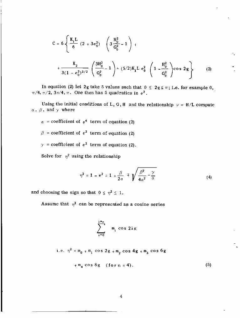
C = 6 I Y 6 (2 + 3eg) (3%- 1) +
In equation (2) let 2g take 5 values such that 0 5 2 g l T ; i.e. for example 0, ~ / 4 , ~ / 2 , 3 ~ / 4 , ~ . One then has 5 quadratics in e 2 .
Using the initial conditions of L, G , H and the relationship v = H/L compute a , p , and y where
a = coefficient of e4 term of equation (2)
p = coefficient of e2 term of equation (2)
y = coefficient of e 2 term of equation (2).
Solve for q2 using the relationship
and choosing the sign so that 0 5 T~ I 1.
Assume that q2 can be represented as a cosine series
i = n
mi cos 2ig c i=O
i.e. q2 = mo t ml cos 2g .+ m2 cos 4 g t m3 c o s 6 g
+ mq C O S 8 g (for n = 4) .
4

Next, construct a 5 X 6 matrix of this shape
70’ = mo t ml t m2 t m3 t m4
q 2 = m + .5 ml - .5 m2 - m3 - .5 m4 1 0
4 = m o - m2 + m4
7; = mo - .5 ml - .5 m2 + m3 - .5 m4
t m2 - m3 m4 7: = m o - m l
Solve for mo . . . m4 using these relationships.
c-
These values of mo . . . m4 are the coefficients of the cosine series that was assumed in equation (5).
b. The Angular Variables
Using the Delaunay set of canonical variables (L, G , H, 4 , g , h ) the equations of motion for the angular variables become:
5
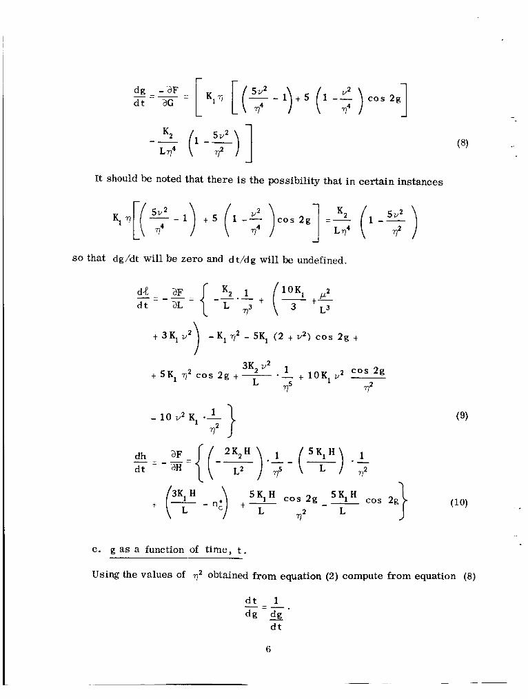
r dg -3F - - - = d t - aG i K l ~ [ ( y - l ) + S (l-:)cos2g]
-- K2 ( l - ? ) ]
L714
It should be noted that there is the possibility that in certain instances
so that dg/dt will be zero and dt/dg will be undefined.
t- d 4 aF d t
L3
+ 3 K 1 v 2 - K, T~ - SK, (2 -+ v2) C O S 2g -+ ) -+ 5 K , T~ C O S 2g t 3K2v2 1 c o s 2g - -+ 10Kl v 2 -.
715 T2
5 K H
L 5K1H c o s 2g 1 (-0s 2g 3K1 H
c. g as a function of time, t . Using the values of 72 obtained from equation (2) compute from equation (8)
d t 1
d t
- - dg - d g -
6
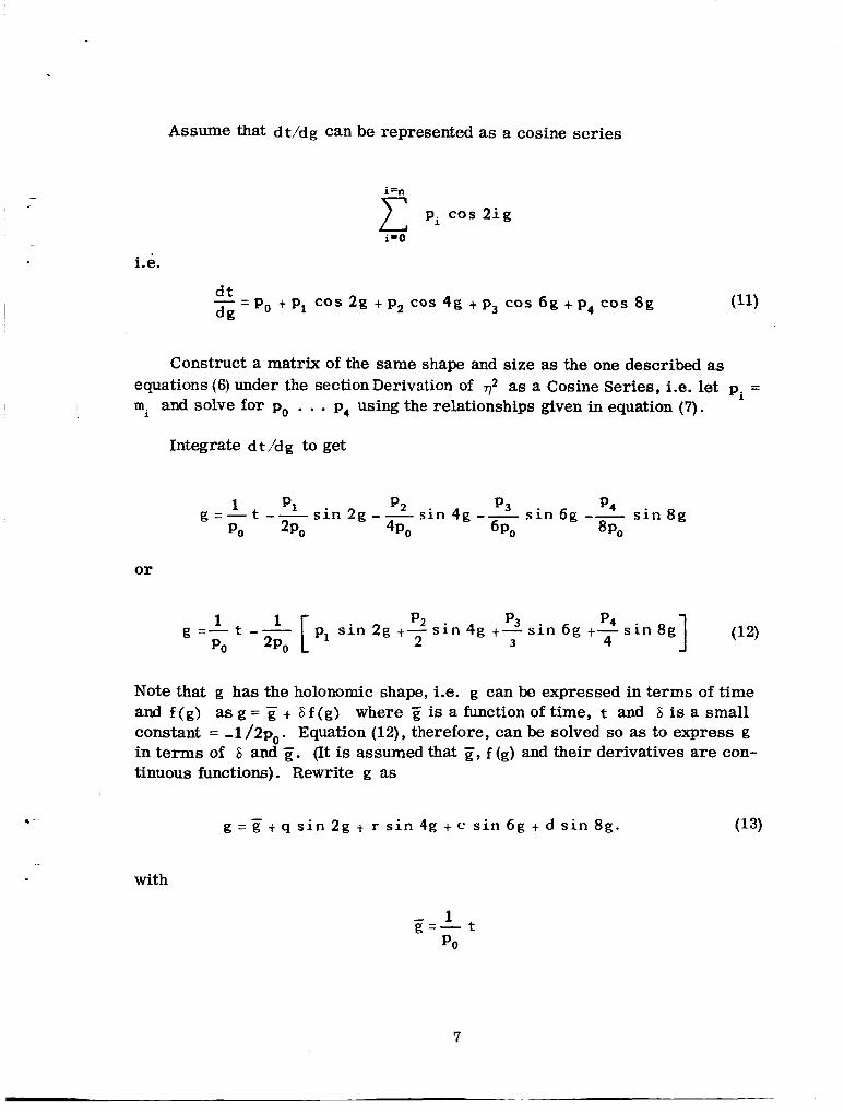
Assume that dt/dg can be represented as a cosine series
i=n
pi cos 2 i g c i=0
i.e.
d t - = P, t P, COS 2g t p2 COS 4g t p3 COS 6 g + P, COS 8 g d g
Construct a matrix of the same shape and size as the one described as equations (6) under the section Derivation of ?* as a Cosine Series, i.e. let pi = mi and solve for po . . . p, using the relationships given in equation (7).
Integrate d t /dg to get
o r
PZ p3 p4
2 3 4 p1 s i n 2g t- s i n 4g t- s i n 6 g t- s i n 8g
1 g =- t -- Po 2po
Note that g has the holonomic shape, i.e. g can be expressed in terms of time and f (g) as g = + 6 f (g) where g is a function of time, t and 6 is a small constant = -1 /2p0. Equation (12), therefore, can be solved so as to express g in te rms of 6 and g . (It is assumed that E, f (g) and their derivatives are con- tinuous functions). Rewrite g as
g = E t q s i n 2 g + r s i n 4g t c s i n 6g t d s i n 8g .
with
7
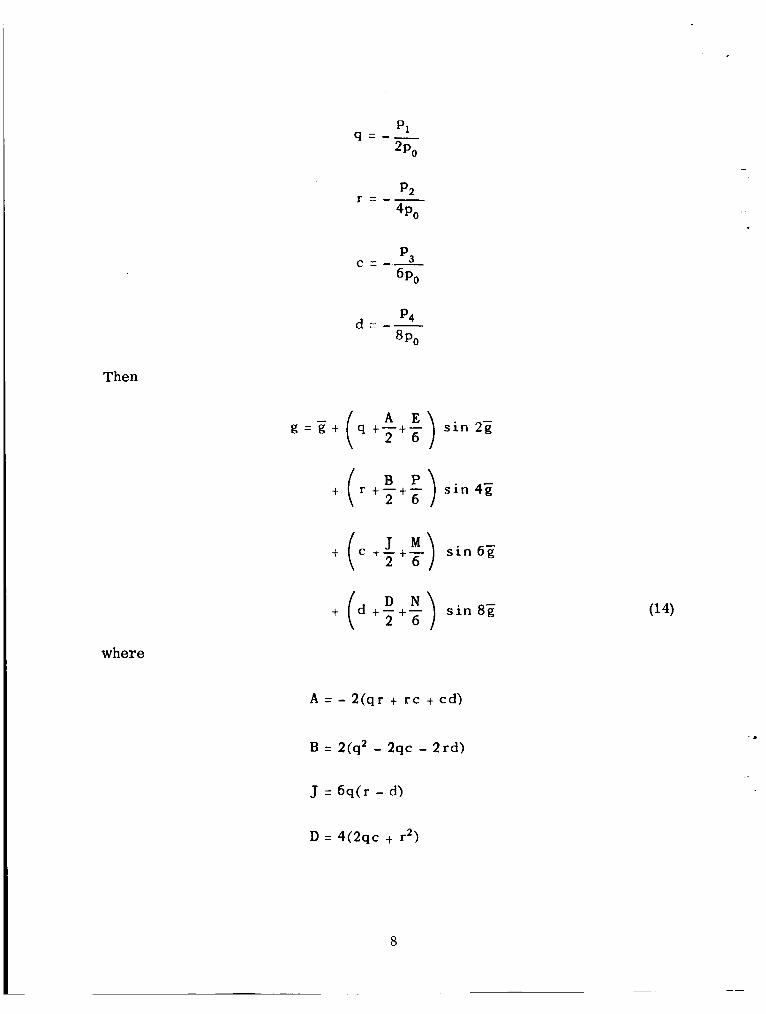
Then
g " E t ( q t-t- : ) s i n 2 2
t ( r t t t i ) s i n 4 2
t ( c tTtF) J M s i n 6 g
t ( d t:t$) s i n 8 2
where
A = - 2(qr t r c t cd)
B = 2(q2 - 2qc - 2rd)
J = 6q(r - d)
D = 4(2qc + r2)
8
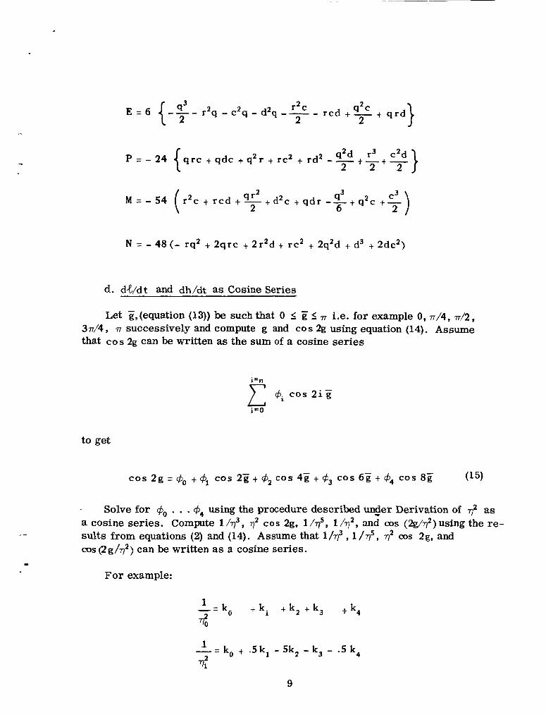
2 E = 6 { -T - q3 2 2 r2 c r q - c q - d2q -- - rcd t
2
.-
N = - 48 (- rq2 t 2qrc t 2r2d t rc2 t 2q2d t d3 t 2dc2)
d. dX/dt and dh/dt as Cosine Series
Let g,(equation (13)) be such that 0 I Z S 7~ i.e. for example 0, ~ / 4 , d 2 , successively and compute g and cos 2g using equation (14). Assume 3n/4,
that C O S 2g can be written as the s u m of a cosine series
to get
.
a cosine series. Compute 1 /q3 , 7' cos 2g, 1 /q5, 1 /q2, and cos (2g/q2) using the re- sults from equations (2) and (14). Assume that l/q3 , 1 /$, q2 cos 2g, and COS (2g/T2) can be written as a cosine series.
Solve for $o . . . 44 using the procedure described under - Derivation of q2 as
For example:
1 -=k, + k i + k 2 + k 3 +k,

1 -= k, <; - k2 + k,
1 -= k, - .5k, - -5k2 t k, - .5k, 4
from which
k3 = - 6 3
1
7 2
k4 =2- k, + k,
- - cos 2g
7, i = O
i = n c ifO
c i -0
i = n
L~ cos 2ig
ki c o s 2ig
D cos 2ig i
10
i"n
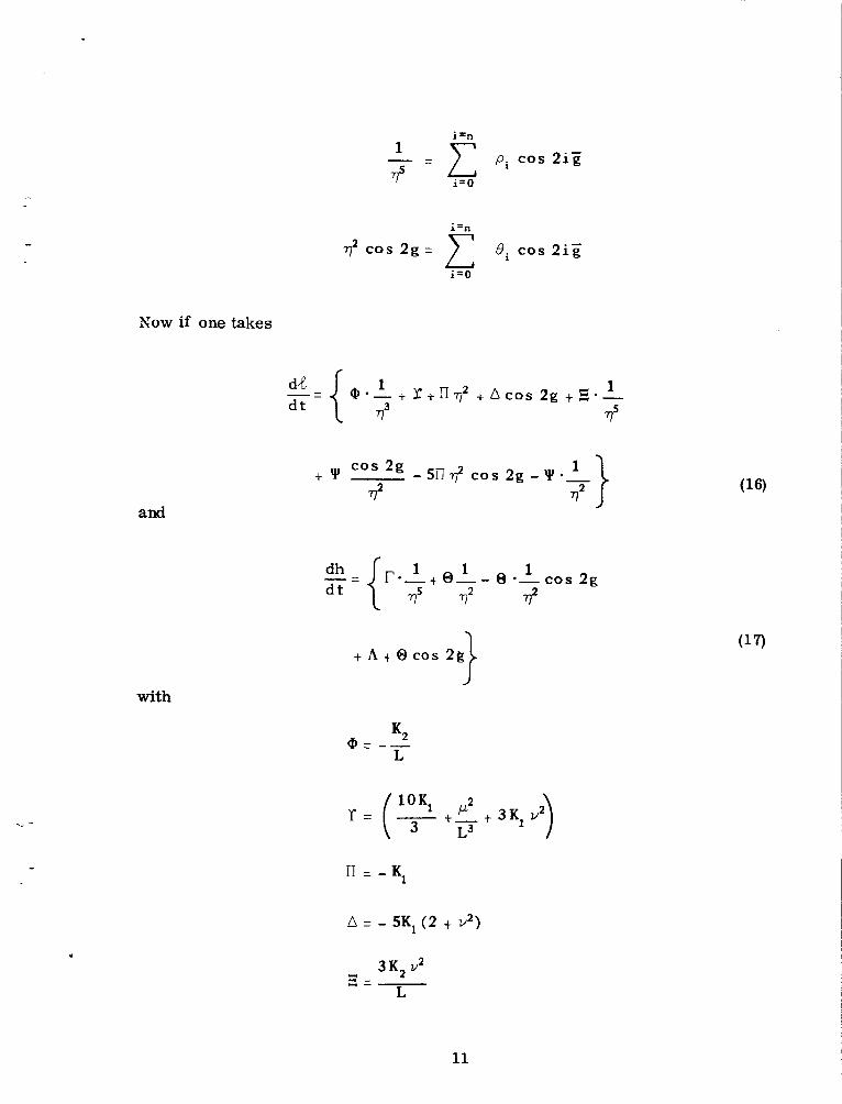
pi cos 2 i g 1
T5 i'0
Now if one takes
and
1 -t h + 8 cos 2g J
with
A = - SKI (2 + v')
I 3K2 v2 C I - L-.--
L
11

Y = 10 K, v2
2 K 2 H
L2 r = -
A = ( T-"$ 3 K , H
then
i = n 1
t mi cos 2 i g + A
i = O i = O
r i = O i = O
Substituting the series in equations (1 8) and (1 9) yields the following expres- sions for dd /d t and dh/d t
12
~
3
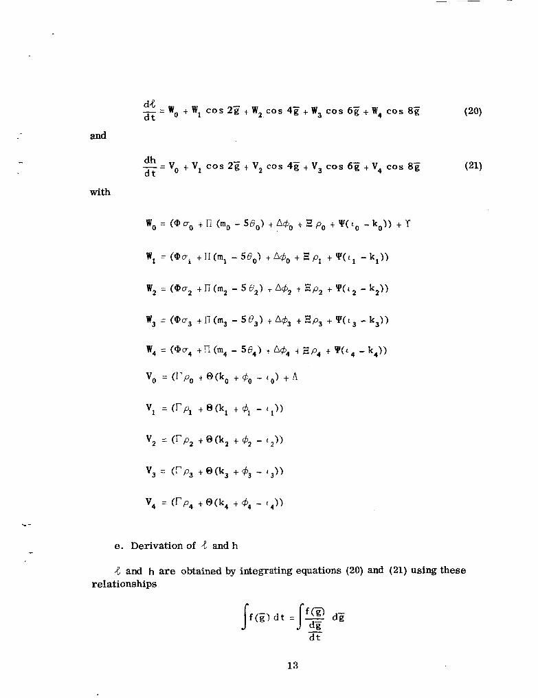
d4 - = W, t W, C O S 2g t W, COS 4g t W, COS 6g t W, COS 8g d t
and
- Vo t V, C O S 2g t V, COS 4g t V, COS 6g t V, cos 8g dh d t --
with
W, =(@vi t r I ( m , -58,) t A 4 0 t E p , t Y ( ( , - k l ) )
W, = (an2 t fl (m, - 5 d 2 ) t 4, t B p2 + Y( L , - k,))
e. Derivation of 4 and h
8 and h are obtained by integrating equations (20) and (21) using these relationships
d t
13
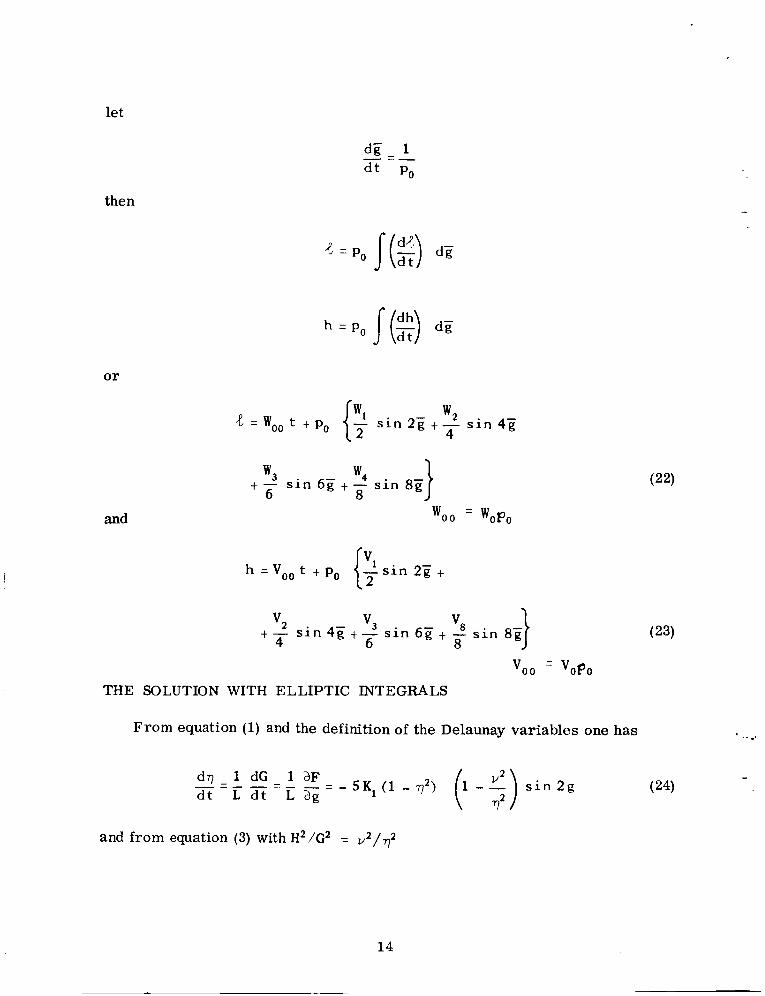
let
then
o r
and -
woo - WOP,
- v o o - VOPO
THE SOLUTION WITH ELLIPTIC INTEGRALS
- -. From equation (1) and the definition of the Delaunay variables one has
_ - - - _ _ d? - 1 dC - 1 d F - = - SK, (1 - 7') (1 - $) s i n 2 g d t L d t L ag
and from equation (3) with H2/C2 = v ~ / ? ~
14

i
1 -
from which one finds
- *K2 (1 -7) t (2 +3e') (1 -5) tKL C
1 5 ( 1 - ? ) (1-5) q3 K,L (26) cos 2g =
Substituting this relationship in equation (24) and using
sin 2 g = * J1 - COS' 2g
d77 - - - - _ - 277- dq2 - dq2 dq d t dq d t d t
one has
now letting q2 = (values of 7' for g = 0) = $
J and
15

when 1 / q 3 is approximated by ( 1 -t- (3/2)e2 + 2e4) and equation (29) is expanded (mglecting pmvers of e grezter thari 8) asing the relationships
and
then
dq2 de2 A,e8 + A3e6 + A 2 e 4 + Ale2 + A ,
d t d t 3 (1 - e’)
with
A 3 = f 5 0 ( v 2 - l ) - 2 [(-4(1-3v2) ($ +I) -$) ($)
A, = { 225 (1 - v ~ ) ~ - { k ( 1 - 3 v 2 ) ($,+J) t$] [ $ ( 1 - 1 2 v 2 ) - 3 1 + ( 1 - 9 v 2 ) - + 1 -- [ (.:I ) GI)}
A, = - 2 [2(1 - 3 v 2 ) ($ + 1) +$] [(1 - 9 ~ ’ ) ($ t I) -&]
16
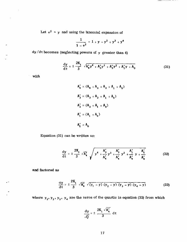
Let e2 = y and using the binomial expansion of
1 - = 1 t Y t Y 2 t Y 3 t Y 4 1 - e2
dy/dt becomes (neglecting powers of y greater than 4)
A;y4 t A;y3 t A;y2 t A ~ Y t A, dY 2Kl -=f- J d t 3
with
Equation (31) can be written as:
-=f - /q dY 2Kl
dt 3
and factored as
where y,, y, , y, , y4 are the zeros of the quartic in equation (32) from which
17
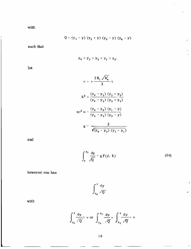
with
such that
Y4 ’ Y3 ’ Y2 ’ Y, ’ Yo. let
(Y4 - Y,> (Y3 - Y,>
(Y4 - Y,> (Y3 - Y,> k2 =
(Y4 - Y,> (Y, - Y>
(y4 - Y,> (Y2 - Y> sn2 u = -
and
however one has
with
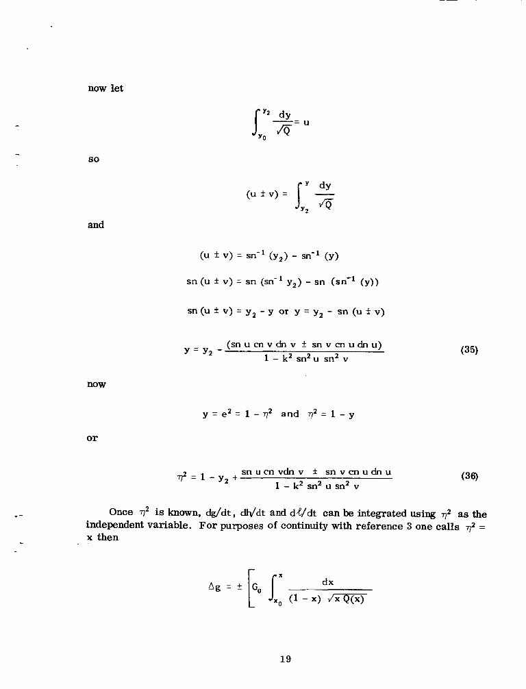
now let
so
and
( s n u c n v d n v f s n v c n u d n u ) 1 - k2 sn2u sn2 v
Y = Y p - (35)
now
or
(36) s n u c n v d n v i s n v c n u d n u 1 - k2 sn2 u sn2 v
? = 1 - y 2 t
Once q2 is known, dg/dt, wdt and dx/dt can be integrated using q2 as the independent variable. For purposes of continuity with reference 3 one calls q2 = x then
19
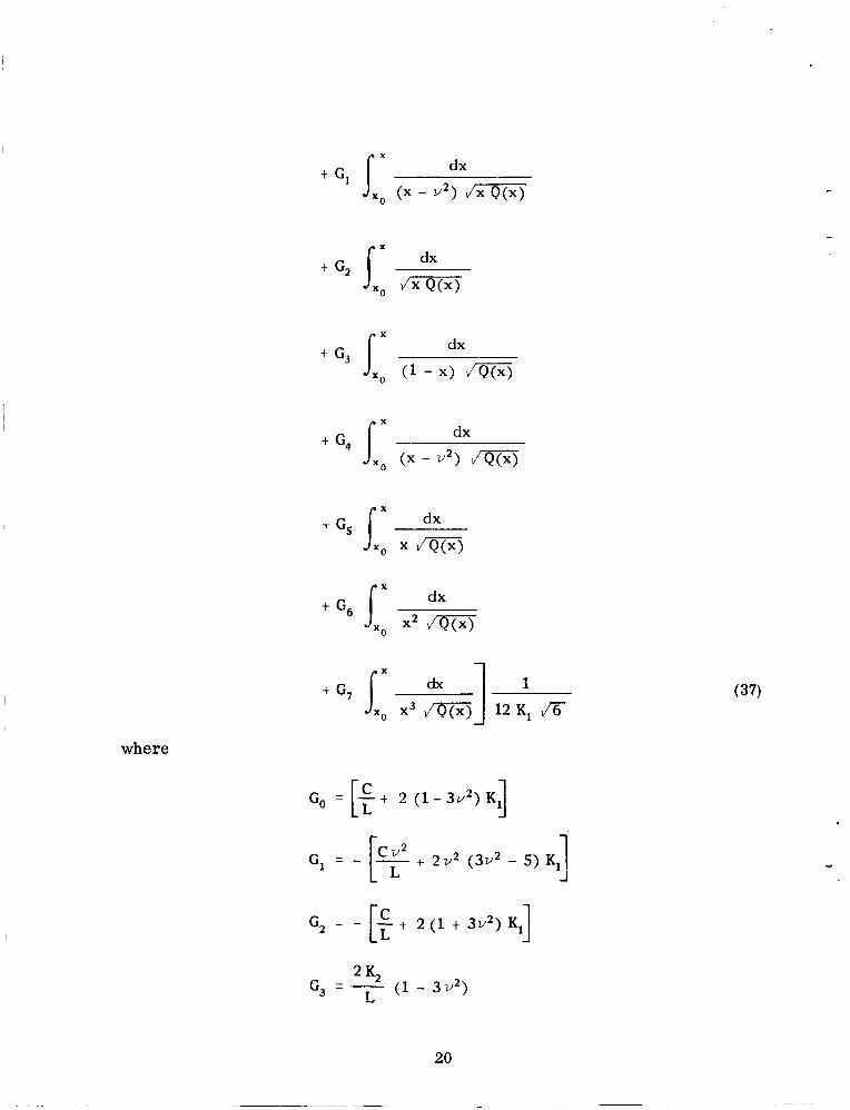
where
L J x 0
dx G3 ( (1 - x) m
Go = [f t 2 ( 1 - 3 u 2 ) KJ
t 2 v 2 (3u2 - 5) K, G, = - 1-I;- c u2
J
G 2 = - [+ t 2 (1 t 3v2) Kl]
(1 - 3v2) K2 G, =- L
20
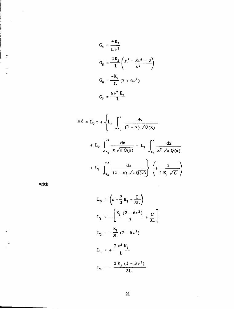
4 % G, = - L u?
(7 + 6 u 2 ) -52 c, =-
L
9u2 K, L G, =-
dx
+ L4 r: (1 - x)
with
3L
L, = - [' (* 3 6u2) t q 3L
K2 L = - - 3L (7 - 6 ~ ' ) 2
7 u2 K2 L
L, = +
2K, ( 1 - 372) L, = -
3L
21

dx
with
H, = (-n', t 2 K, v)
3
where
The integrals needed are of two types:
I. Integrals involving m)
for
and
dx 1. c
dx
2. s (u2 - x) J w )
see reference 5 page 102 # 251.39
22
-.

r d I d t
with m = 1
see #340.01 page 205 reference 5
with
a; =
( a - c ) ( d - t ) ( a - d ) (c- t )
sn2 u =
2
/(a - c ) (b - d) g =
a - d a - c
a2 = -, = F (cp, k)
23

for
dx 5.
see reference 5 page 99 No. 251.04
fd d t - I,, t" / (a - t ) (h - t ) (c - t ) (d - t )
2 I' (1 - a' sn2 u)" du d" (1 - a i sn2 u)"
with
1 = a i sn2 u t = d ( 1 - a2 sn2 u )
with m = 1
see #340.01 page 205 reference 5
m = 1, 2, 3.
- g [(ai - a2) n(cp, ai, k) t a2 P] ai d
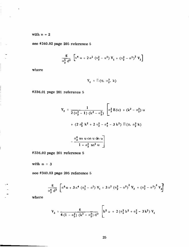
withm=2
see #340.02 page 205 reference 5
- g [u4 u t 2a2 (u; - a2) v, t (a; - a2)2 v2] a: d2
where
#336.01 page 201 reference 5
Q; E(u) t (k2 - a:) u c 1 2 (ai - 1) (k2 - a;)
v, =
a: sn u cn u dn u
1 - a: sn2 u 1 -
f336.02 page 201 reference 5
w i t h m = 3
see #340.03 page 205 reference 5
2 a6u + 3u4 (“2’ - a2) v, t 3a2 (u; - 2) v, + (a; - 4 3 VJ “C a6 2 d3
where
F2 u -+ 2 fn? E2 + a: - 3k2) V, g
4 (1 - ai) (k2 - a;) d3 \ -<2 - v, =
25

a; sn u cn u dn
( 1 - ai sn2 u) 2 I t 3 (u; - 2a2, k2 - 2a: t 3k2) V, t
#336.03 page 201 reference 5 ,
II. Integrals involving v ' Z @ i j
dx i(1 - x) ham
10. J dx
x2 hm3
For these integrals one fits, by the method of least squares, a polynomial of degree 2 to the expression for x Q(x), (0 I x I x4). The procedure is
1. Map z = x (x - XI) (x - x2) (x - x3) (x - x4)
ir?to
26
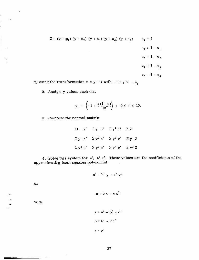
a2 = 1 - x1
a3 - 1 - x2
a4 = 1 - x3
-
a5 1 - x4
by using the transformation x = y + 1 with - 1 L y I - as
2. Assign y values such that
; 0 1 i 5 10. yi = (-1 t i (1 - e ) 10
3. Compute the normal matrix
11 a' Z y b' Z y 2 c' Z Z
Z y a' Z y 2 b ' X y 3 c' .Ty Z
y2 a' 2 y3 b' 1 y4 c' 2 y2 Z
4. Solve this system for a', b' c'. These values are the coefficients of the approximating least squares polynomial
a' t b' y t c' y2
or
with
a t b x + c x 2
a = a' - b' t c'
u - u - 2 c '
c = c'
L. - L'
27
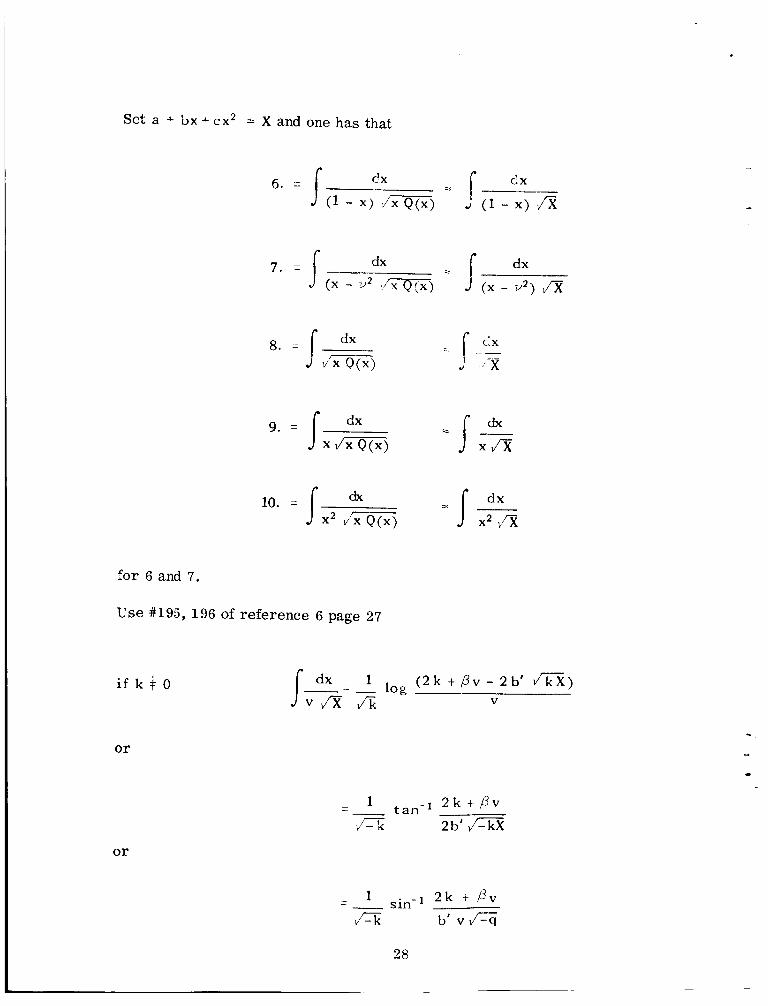
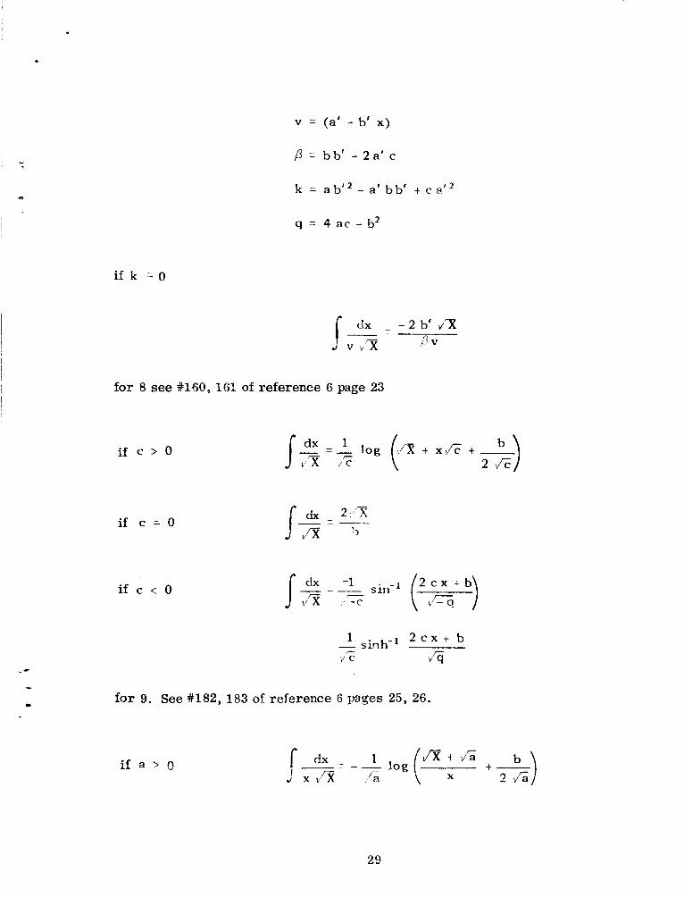
Set a + bx + c x 2 = X and one has that
6 . = C?X ClX
for 6 and 7.
U s e #195, 196 of reference 6 page 27
i f k i O
o r
or
(2 k t P v - 2 b' J k j z ) V
1 1 2 k t p v - -- t a n -
V G 2b' m x
- 1 1 2 k t P v __ sin- J-=i; b' v f i
-
28
c
v = (a' + b' x)
p = bb' - 2 a' c
k = a b t 2 - a 'bb ' t ce'*
q = 4 a c - b 2
i f k = O
for 8 see #160, I61 of reference 6 page 23
i f c > O
if c = O
i f c < O dx - -1 2 c x + b
1 2 c x t b - sirlh-' J;i F
d C
for 9. See #182, 183 of reference G pages 25, 26.
I f a > ( !
29

if a = O
if a < O
or
2 ss= - -a bx
_ _ 1 sinh-l ( 2a t ~ bx ) Jz;
for 10. See #186 of reference 6 page 26.
An example of the fitting procedure is as follows:
let
x1 = .53 xg = . 23
x2 = .31 x4 = . 12
or
a = 1 c = .69
b = .47 d = . 7 7
e = .88
such that
y = -1 , - .988 , - . 9 7 6 . . -.88
and the normal matrix is
Ila' -10.34b' 9 .73544~' 4.8922239 x
-10. %a' 9.73544b' -9.1810928~' -4.6383256 x
9.73544a' -9.1810928b' 8.672256%' 4.4007739 x 10-
30

w k s e solution gives as t ~ e approximate formula
Z 2 (17f3.92728 -378.13508 y -199.80525 y 2 )
Z 2 (.30355 121.474220 x-199.80525 z 2 ) lo-’
The original value of 2 and those obtained by substitution in the approximatinc. ‘nrmula are plotted below.
i 0 0 . O r x
! X
f
C d
X
? 0 I
X APPROX I M A T I Y G VALUES 5
i
1 0
I
X
00 - ~ _ _
1 I I i
I I - c! 952 -0.928 - 0.904 - 0.880 - 1.090 - 0.976
v
31
REFERENCES AND EIBii0GIiAPH-Y
1. Frost, Frances A., Long Term Mal-m of a Lunar Satellite, GSFC X-547-65-388 October 1965. w
2. Brown, E. W . , "The Stellar Problem of Three Bodies", Monthly notices of the Royal Astronomical Society Vol. 97, 56-66, 116-127, 388-395 (1936).
-
3. Giacaglia, Georgio E . O., Murphy, James P., and Felsentreger, Theodore L. in Colloboration with Standish, E., Myles, Jr. and Velez, Carmelo E. , , - The Motion of a Satellite of the Moon, GSFC X-547-65-218, June 1965.
4. Kozai, Y., "Motion of a Lunar Orbiter", Journal of the Astronomical Society of Japan, Vol. 15, 301-31 (1963).
5. Byrd, P., and Friedman, M., Handbook of Elliptic Integrals for Engineers and Physicists, Springer-Verlag, 1954.
6. A Short Table of Integrals, by B. 0. Peirce, Ginn and Co. 1910.
32