Embed Size (px)
Citation preview

HAL Id: hal-01025814https://hal-mines-paristech.archives-ouvertes.fr/hal-01025814
Submitted on 3 Jan 2017
HAL is a multi-disciplinary open accessarchive for the deposit and dissemination of sci-entific research documents, whether they are pub-lished or not. The documents may come fromteaching and research institutions in France orabroad, or from public or private research centers.
L’archive ouverte pluridisciplinaire HAL, estdestinée au dépôt et à la diffusion de documentsscientifiques de niveau recherche, publiés ou non,émanant des établissements d’enseignement et derecherche français ou étrangers, des laboratoirespublics ou privés.
Computation of Phase Transformation Paths in Steelsby a Combination of the Partial- and Para-equilibrium
Thermodynamic ApproximationsTakao Koshikawa, Charles-André Gandin, Michel Bellet, Hideaki Yamamura,
Manuel Bobadilla
To cite this version:Takao Koshikawa, Charles-André Gandin, Michel Bellet, Hideaki Yamamura, Manuel Bobadilla.Computation of Phase Transformation Paths in Steels by a Combination of the Partial- and Para-equilibrium Thermodynamic Approximations. ISIJ international, Iron & Steel Institute of Japan,2014, 54 (6), pp.1274-1282. �10.2355/isijinternational.54.1274�. �hal-01025814�
© 2014 ISIJ 1274
ISIJ International, Vol. 54 (2014), No. 6, pp. 1274–1282
Computation of Phase Transformation Paths in Steels by a Combination of the Partial- and Para-equilibrium Thermodynamic Approximations
Takao KOSHIKAWA,1,2)* Charles-André GANDIN,1) Michel BELLET,1) Hideaki YAMAMURA3) andManuel BOBADILLA4)
1) MINES ParisTech & CNRS, CEMEF UMR 7635, 06904 Sophia Antipolis, France.2) Nippon Steel & Sumitomo Metal Corporation, Oita Works Equipment Division, 1 Oaza-Nishinosu, Oita City, Oita Prefecture,870-0992 Japan. 3) Nippon Steel & Sumitomo Metal Corporation, Steelmaking R&D Division, 20-1 Shintomi, Futtsu City,Chiba Prefecture, 293-8511 Japan.4) ArcelorMittal Maizières, Research and Development, BP 30320, 57283 Maizières-lès-Metz Cedex, France.
(Received on August 29, 2013; accepted on February 13, 2014)
A model combining the partial-equilibrium and para-equilibrium thermodynamic approximations is pre-sented. It accounts for fast diffusion of interstitial elements, such as carbon, and low diffusion of substi-tutional elements in the solid phases, while complete mixing is assumed for all elements in the liquidphase. These considerations are turned into classical mathematical expressions for the chemical poten-tials and the u-fractions, to which mass conservation equations are added. The combination of the twomodels permits application to steels, dealing with partial-equilibrium for solidification and para-equilibriumfor both the δ -BCC to γ-FCC peritectic transformation and the γ-FCC to α-BCC solid state transformation.The numerical scheme makes use of calls to Thermo-Calc and the TQ-interface for calculating thermody-namic equilibrium and accessing data from the TCFE6 database. Applications are given for a commercialsteel. The results are discussed based on comparison with classical microsegregation models and exper-imental data.
KEY WORDS: solidification; microsegregation; partial-equilibrium; para-equilibrium; peritectic transformation.
1. Introduction
Average alloy properties in multiphase temperature inter-vals are important for thermomechanical process simula-tions. Numerical tools have been developed to follow thetransformation paths based on thermodynamic consider-ations. Two classical limits are routinely computed: thelever rule (LR) approximation and the Gulliver-Scheil (GS)approximation.1,2) For LR, full equilibrium is assumed,meaning that all chemical elements can diffuse rapidly. Incontrast, the GS approximation neglects diffusion in solidphases where elements are completely frozen. In practice,most industrial steels include interstitial and substitutionalelements. Interstitial elements, such as carbon, have highdiffusivity in the solid phase while substitutional elementshave low diffusivity. Thus, the above LR and GS approxi-mations do not fully apply. To overcome this problem, thepartial-equilibrium (PE) approximation3,4) has been devel-oped. PE is intended to take into account perfect diffusionof interstitial elements but no diffusion of substitutional ele-ments. However, the peritectic transformation often encoun-tered in commercial alloys cannot take place if only PE is
considered. This limitation could be circumvented by a LRtreatment of the δ-BCC (or δ-ferrite)/γ-FCC (or γ-austenite)mixture during the peritectic transformation,5) thus permit-ting the activation of the δ-BCC to γ-FCC phase transfor-mation. This will be later refereed as PE + LR solidificationpath. It is to be mentioned that, while in agreement withobservations, no experimental quantitative data is yet avail-able that could be directly compared with predicted kineticsof the peritectic phase transformation. The LR treatment ofthe peritectic transformation is also a very crude approxima-tion that does not fix the problem in coherent manner withrespect to the PE approximation.
In the present study, a new numerical scheme is presentedfor the computation of phase transformations in steels. Itis coupled with thermodynamic equilibrium calculationsbased on call to the software Thermo-Calc6) through theTQ-interface using the TCFE6 database.7) The so-calledpara-equilibrium (PA) approximation presented by Hillert8)
has been introduced to deal with the peritectic reaction dur-ing a PE solidification path, later refereed as PE + PAapproximation. This is implemented in previous develop-ments presented by Zhang et al.4) for the computation of LR,GS and PE + LR solidification paths. Because PA was ini-tially developed for solid state transformations, it is alsoused to simulate phase transformations during cooling expe-
* Corresponding author: E-mail: [email protected]: http://dx.doi.org/10.2355/isijinternational.54.1274
ISIJ International, Vol. 54 (2014), No. 6
1275 © 2014 ISIJ
rienced during steel processing after solidification. Thenumerical scheme is applied to steel alloys experiments alsopresented in this contribution.
2. Experiments
2.1. Unidirectional Solidification ExperimentTo investigate solidification path in Fe–C–Mn–S–Si–P–
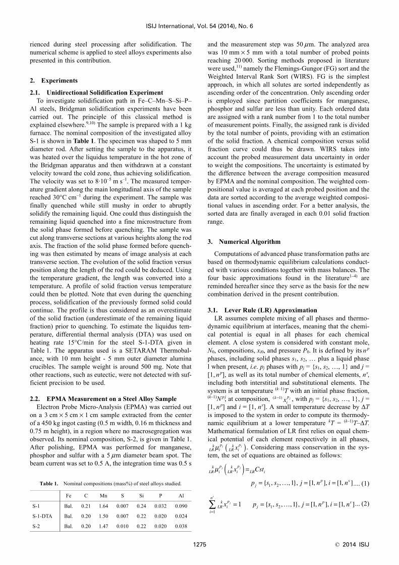
Al steels, Bridgman solidification experiments have beencarried out. The principle of this classical method isexplained elsewhere.9,10) The sample is prepared with a 1 kgfurnace. The nominal composition of the investigated alloyS-1 is shown in Table 1. The specimen was shaped to 5 mmdiameter rod. After setting the sample to the apparatus, itwas heated over the liquidus temperature in the hot zone ofthe Bridgman apparatus and then withdrawn at a constantvelocity toward the cold zone, thus achieving solidification.The velocity was set to 8·10–5 m s–1. The measured temper-ature gradient along the main longitudinal axis of the samplereached 30°C cm–1 during the experiment. The sample wasfinally quenched while still mushy in order to abruptlysolidify the remaining liquid. One could thus distinguish theremaining liquid quenched into a fine microstructure fromthe solid phase formed before quenching. The sample wascut along transverse sections at various heights along the rodaxis. The fraction of the solid phase formed before quench-ing was then estimated by means of image analysis at eachtransverse section. The evolution of the solid fraction versusposition along the length of the rod could be deduced. Usingthe temperature gradient, the length was converted into atemperature. A profile of solid fraction versus temperaturecould then be plotted. Note that even during the quenchingprocess, solidification of the previously formed solid couldcontinue. The profile is thus considered as an overestimateof the solid fraction (underestimate of the remaining liquidfraction) prior to quenching. To estimate the liquidus tem-perature, differential thermal analysis (DTA) was used onheating rate 15°C/min for the steel S-1-DTA given inTable 1. The apparatus used is a SETARAM Thermobal-ance, with 10 mm height - 5 mm outer diameter aluminacrucibles. The sample weight is around 500 mg. Note thatother reactions, such as eutectic, were not detected with suf-ficient precision to be used.
2.2. EPMA Measurement on a Steel Alloy SampleElectron Probe Micro-Analysis (EPMA) was carried out
on a 3 cm × 5 cm × 1 cm sample extracted from the centerof a 450 kg ingot casting (0.5 m width, 0.16 m thickness and0.75 m height), in a region where no macrosegregation wasobserved. Its nominal composition, S-2, is given in Table 1.After polishing, EPMA was performed for manganese,phosphor and sulfur with a 5 μm diameter beam spot. Thebeam current was set to 0.5 A, the integration time was 0.5 s
and the measurement step was 50 μm. The analyzed areawas 10 mm × 5 mm with a total number of probed pointsreaching 20 000. Sorting methods proposed in literaturewere used,11) namely the Flemings-Gungor (FG) sort and theWeighted Interval Rank Sort (WIRS). FG is the simplestapproach, in which all solutes are sorted independently asascending order of the concentration. Only ascending orderis employed since partition coefficients for manganese,phosphor and sulfur are less than unity. Each ordered dataare assigned with a rank number from 1 to the total numberof measurement points. Finally, the assigned rank is dividedby the total number of points, providing with an estimationof the solid fraction. A chemical composition versus solidfraction curve could thus be drawn. WIRS takes intoaccount the probed measurement data uncertainty in orderto weight the compositions. The uncertainty is estimated bythe difference between the average composition measuredby EPMA and the nominal composition. The weighted com-positional value is averaged at each probed position and thedata are sorted according to the average weighted composi-tional values in ascending order. For a better analysis, thesorted data are finally averaged in each 0.01 solid fractionrange.
3. Numerical Algorithm
Computations of advanced phase transformation paths arebased on thermodynamic equilibrium calculations conduct-ed with various conditions together with mass balances. Thefour basic approximations found in the literature1–4) arereminded hereafter since they serve as the basis for the newcombination derived in the present contribution.
3.1. Lever Rule (LR) ApproximationLR assumes complete mixing of all phases and thermo-
dynamic equilibrium at interfaces, meaning that the chemi-cal potential is equal in all phases for each chemicalelement. A close system is considered with constant mole,N0, compositions, xi0, and pressure P0. It is defined by its n p
phases, including solid phases s1, s2, … plus a liquid phasel when present, i.e. pj phases with pj = {s1, s2, …, 1} and j =[1, n p], as well as its total number of chemical elements, ns,including both interstitial and substitutional elements. Thesystem is at temperature (k–1)T with an initial phase fraction,(k–1)N pj, at composition, , with pj = {s1, s2, …, 1}, j =[1, n p] and i = [1, ns]. A small temperature decrease by ΔTis imposed to the system in order to compute its thermody-namic equilibrium at a lower temperature kT = (k–1)T–ΔT.Mathematical formulation of LR first relies on equal chem-ical potential of each element respectively in all phases,
. Considering mass conservation in the sys-tem, the set of equations are obtained as follows:
.... (1)
... (2)
Table 1. Nominal compositions (mass%) of steel alloys studied.
Fe C Mn S Si P Al
S-1 Bal. 0.21 1.64 0.007 0.24 0.032 0.090
S-1-DTA Bal. 0.20 1.50 0.007 0.22 0.020 0.024
S-2 Bal. 0.20 1.47 0.010 0.22 0.020 0.038
( )kipx j−1
LRk
ip
LRk
ipj jxμ ( )
LRk
ip
LRk
ip
LR i
jp s
j jx Cst
p s s j n i n
μ ( ) =
= = ={ , , , }, [ , ], [ , ]1 2 1 1 1…
LRk
ip
i
n
jp sx p s s j n i nj
s
=∑ = = = =
11 21 1 1 1{ , , , }, [ , ], [ , ]…
© 2014 ISIJ 1276
ISIJ International, Vol. 54 (2014), No. 6
.. (3)
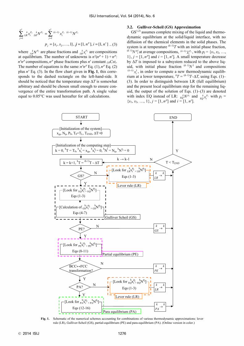
where are phase fractions and are compositionsat equilibrium. The number of unknowns is ns(n p + 1) + n p:nsn p compositions, n p phase fractions plus ns constant LRCsti.The number of equations is the same: nsn p Eq. (1), n p Eq. (2)plus ns Eq. (3). In the flow chart given in Fig. 1, this corre-sponds to the dashed rectangle on the left-hand-side. Itshould be noticed that the temperature step ΔT is somewhatarbitrary and should be chosen small enough to ensure con-vergence of the entire transformation path. A single valueequal to 0.05°C was used hereafter for all calculations.
3.2. Gulliver-Scheil (GS) ApproximationGS1,2) assumes complete mixing of the liquid and thermo-
dynamic equilibrium at the solid/liquid interface, with nodiffusion of the chemical elements in the solid phases. Thesystem is at temperature (k–1)T with an initial phase fraction,(k–1)N pj, at average compositions, , with pj = {s1, s2, …,1}, j = [1, n p] and i = [1, ns]. A small temperature decreaseby ΔT is imposed to a subsystem reduced to the above liq-uid, with initial phase fraction (k–1)N 1 and compositions
, in order to compute a new thermodynamic equilib-rium at a lower temperature, kT = (k–1)T–ΔT, using Eqs. (1)–(3). In order to distinguish between LR (full equilibrium)and the present local equilibrium step for the remaining liq-uid, the output of the solution of Eqs. (1)–(3) are denotedwith index EQ instead of LR: and with pj ={s1, s2, …, 1}, j = [1, n p] and i = [1, ns].
LRk
ip
j
n
LRk p k
ip k
j
np
j
x N x N
p s s
j
p
j j
p
j
=
− −
=∑ ∑=
=1
1 1
1
1 2 1
( ) ( )
{ , , , },… jj n i np s= =[ , ], [ , ]1 1
LRk pN j
LRk
ipx j ( )k
ip
x j−1
( )kix
−1 1
EQk pN j
EQk
ipx j
Fig. 1. Schematic of the numerical schemes accounting for combinations of various thermodynamic approximations: leverrule (LR), Gulliver-Scheil (GS), partial-equilibrium (PE) and para-equilibrium (PA). (Online version in color.)
ISIJ International, Vol. 54 (2014), No. 6
1277 © 2014 ISIJ
Because of the absence of diffusion in the solid phasesunder the GS approximation, the average solid compositionof the entire system at temperature kT is directly computedby adding the fraction of solid formed during cooling of thesubsystem to the already existing solid using:
... (4)
The new total fraction of the solid phases for the entiresystem is equal to:
..... (5)
Liquid fraction and composition are simply given by theequilibrium solution:
....... (6)
............................... (7)
3.3. Partial-equilibrium (PE) ApproximationThe PE approximation is intended to be used for systems
with large differences in the diffusivity of chemicalelements. This is typically the case in steels containing inter-stitial elements with high diffusivity and substitutionalelements with low diffusivity. It is seen as an extension ofthe GS approximation and was initially developed for sim-ulation of the solidification paths in steels3,4) where carbonis interstitial and diffuses rapidly compared to e.g., substitu-tional chromium. To simplify the problem, carbon is the onlyinterstitial element considered in this study. Mathematicalformulation of PE first relies on equal average chemicalpotential of carbon in all phases, . It also con-siders unchanged values for the average u-fractions of the sub-stitutional elements defined by with respect to the values provided by the last GS step attemperature kT for each phase participating to equilibrium,
. These conditions are added themass conservation of carbon and of all the substitutional ele-ments over all participating phases considering the valuesprovided by the last GS step at temperature kT. Thus, PE isinitialized from a GS calculation as shown in Fig. 1. Theabove four considerations translate into:
.... (8)
... (9)
.... (10)
..... (11)
The number of unknowns is (ns + 1)n p + 1: (nsn p) compo-sitions, n p phase fractions plus the constant PECst. The num-ber of equations is the same: n p Eq. (8), (ns–1)n p Eqs. (9),(10) plus n p Eq. (11).
3.4. Para-equilibrium (PA) ApproximationOn the basis of Hillert’s idea,8) the PA approximation was
originally developed for a transformation taking placebetween solid phases with local equilibrium at the phaseinterface and frozen composition of substitutional elements.It permits to deal with solid phase transformation with thesame u-fraction of substitutional elements and equality ofchemical potential for instertitial elements. The condition onthe interstitial element thus writes similarly as for the PEapproximation with equal average chemical potentialsamong solid phases. This means that diffusion of interstitialelements is assumed very high, as for PE. For substitutionalelements, condition is given on the summation of the prod-uct of the average chemical potential by the average u-frac-tion which is deduced from no driving force on the interface.A detailed derivation is given in Ref. 8). As stated before,it is chosen to consider a unique average u-fraction for eachsubstitutional element in all the solid phases, , i = [1,ns], its value being defined below. Finally, as for previousapproximations, mass conservation of interstitial and substi-tutional elements over all solid phases must also be verified.Considering only carbon as the interstitial element, the fol-lowing set of equations must thus be satisfied:
.... (12)
.... (13)
..... (14)
...... (15)
..... (16)
The number of unknown compositions is (ns + 1) n p +2: (nsn p) compositions, n p phase fractions plus the constantsPACst1 and PACst2. The number of equations is the same: n p
Eq. (12), n p Eq. (13), n p(ns–1) Eqs. (14), (15) plus Eq. (16).Comparing the set of equations for PA to PE approxima-tions, the main difference appears through Eq. (13). In theliterature, application of the PA approximation is usuallylimited to 2 solid phases. The above PA set of equationscan be solved for a subsystem made of two solid phasespj = {s1, s2} undergoing a peritectic reaction, in whichcase this subsystem is extracted from a previous PE cal-
GSk
ip k p k
ip
EQk p
EQk
ip
k
x N x N x
N
j j j j j≠ − ≠ − ≠ ≠ ≠
−
= +( )1 1 1 1 1 1 1
1
( ) ( )
( )
/
ppEQk p p sj jN j n i n
≠ ≠+( ) = =1 1 1 1[ , ], [ , ]
GSk p k p
EQk p p sN N N j n i nj j j≠ − ≠ ≠= + = =1 1 1 1 1 1( ) [ , ], [ , ]
GSk
i EQk
isx x i n1 1 1= = [ , ]
GSk
EQkN N1 1=
PEk
Cp
PEk
ipj jxμ ( )
PEk
i Cp
PEk
i Cp
PEk
Cpu x xj j j
≠ ≠= −( )/ 1
GSk
i Cp
GSk
i Cp
GSk
Cpu x xj j j
≠ ≠= −( )/ 1
PEk
Cp
PEk
ip
PE
jp s
j jx Cst
p s s j n i n
μ ( ) =
= = ={ , , , }, [ , ], [ , ]1 2 1 1 1…
PEk
i Cp
GSk
i Cp
jp su u p s s j n i nj j
≠ ≠= = = ={ , , , }, [ , ], [ , ]1 2 1 1 1…
PEk
Cp
j
n
PEk p
GSk
Cp
j
n
GSk p
j
x N x N
p s s j
j
p
j j
p
j
= =∑ ∑=
= =1 1
1 2 1 1{ , , , }, [… ,, ]np
PEk
i Cp
i
n
PEk p
GSk
i Cp
i
n
GSk p
j
x N x N
p s s
j
s
j j
s
j
≠=
≠=
∑ ∑=
=1 1
1 2 1{ , , , },… jj n i np s= =[ , ], [ , ]1 1
PEk
i Cpu ≠
PAk
Cp
PAk
ip
PA
jp s
j jx Cst
p s s j n i n
μ ( ) =
= = =
1
1 11 2{ , , }, [ , ], [ , ]…
PAk
i Cp
PAk
i Cp
PAk
ip
j
n
PA
j
u x Cst
p s s j
j j j
p
≠ ≠=
( ) =
= =
∑ μ1
1 2
2
1{ , , }, [ ,… nn i np s], [ , ]= 1
PAk
i Cp
PEk
i Cp
jp su u p s s j n i nj
≠ ≠= = = ={ , , }, [ , ], [ , ]1 2 1 1…
PAk
Cp
j
n
PAk p
PEk
Cp
j
n
PEk p
j
x N x N
p s s j n
j
p
j j
p
j
= =∑ ∑=
= =1 1
1 2 1{ , , }, [ ,… pp ]
PAk
i Cp
i
n
PAk p
j
n
PEk
i Cp
i
n
PEk p
j
n
j
x N x N
p
j
s
j
p
j
s
j
p
≠==
≠==
∑∑ ∑∑=
=11 11
{{ , , }, [ , ], [ , ]s s j n i np s1 2 1 1… = =

© 2014 ISIJ 1278
ISIJ International, Vol. 54 (2014), No. 6
culation, thus explaining the index PE used in the aboveEqs. (14)–(16). For the u-fraction, it is to be noticed that anaverage value is defined, where
. It is thus computed for
the subsystem of the phases considered under PA. It is alsoworth noticing that when only solid phases coexist, a simplelever rule calculation can be used for initialisation.
Thus, PA provides with a local equilibrium condition atan interface that differs from LR or full equilibrium. PA andLR applied at a solid/solid interface can thus be combinedwith the PE approximation used to deal with a solid/liquidinterface.
3.5. Numerical SchemeThe numerical scheme for a general cooling sequence
during solidification is shown in Fig. 1. Several combina-tions of the above approximations are possible:
• LR (i.e., not GS in Fig. 1). It obviously corresponds tofull thermodynamic equilibrium transformation pathsand is valid from a temperature higher than the liquidustemperature up to room temperature.
• GS (i.e., not PE in Fig. 1). As explained above, itimplies that all interstitial and substitutional elementsin all solid phases are frozen, not permitting the peri-tectic reaction to take place. Because such approxima-tion is difficult to maintain up to low temperature, acritical fraction of liquid (0.0001%) is chosen to stopthe transformation, below which the average composi-tion of all phases is kept constant: and .
• PE (i.e., not BCC↔FCC in Fig. 1). Considered alone,it considers full equilibrium of interstitials while sub-stitutional elements are frozen. This does change thesolidification path compared to GS, yet still not permit-ting the peritectic reaction to occur.
• PE + LR (i.e., not PA in Fig. 1). It keeps the PE approx-imation while handling the peritectic reaction by usinga simple LR approximation among the δ -BCC andγ-FCC solid phases.5) Note that the γ-FCC to α-BCCsolid state transformation is considered in such situa-tion.
• PE + PA (i.e., PA in Fig. 1). This configuration pro-vides with the most advanced configuration where theδ -BCC to γ-FCC peritectic transformation and theγ-FCC to α-BCC solid state transformation are bothconsidered under PA conditions.
4. Application to Steel Alloys and Discussion
4.1. Solidification Path for S-1The measured liquidus temperature by means of DTA and
the calculated one are shown in Table 2. The calculated val-ue based on thermodynamic equilibrium is slightly lowerthan measurement. It is yet within the uncertainty of theexperimental method. During DTA, the temperature differ-ence between the alloy sample and a reference sample isrecorded during heating to reveal the latent heat requiredduring melting. Such a phase transformation, however,needs a driving force leading to overheating of the sample
to transform the solid into liquid, and hence uncertainty inthe determination of the liquidus temperature. The otherpossible reason is inherent to the precision of the thermo-couples and the accuracy of the thermodynamic database.Overall, the comparison is thus considered as very good.
Figure 2(a) shows calculated solidification paths as afunction of temperature for composition S-1. Figures 2(b)and 2(c) present the same results for smaller temperatureintervals. Measurements data are added in Figs. 2(a) and2(b). Differences clearly appear between computationsusing the various approximations. All simulations yet liewithin the LR and GS curves. This was indeed expectedsince, in the absence of undercooling, LR and GS could beregarded as the two extreme thermodynamic limits withrespect to solid state diffusion. Under LR, the total solid
PEk
i Cp
PEk
i Cp
PEk
Cpu x x≠ ≠= −( )/ 1
PEk
i Cp
PEk
i Cp
PEk p
j
n
PEk p
j
n
x x N Nj j
p
j
p
≠ ≠= =
= ∑ ∑1 1
/
GSk
ip k
ipx xj j≠ − ≠=1 1 1( )
GSk p k pN Nj j≠ − ≠=1 1 1( )
Table 2. Liquidus temperature (°C) and onset temperature for theperitectic transformation (°C) deduced from DTA mea-surement and from the TCFE6 database11) for alloy S-1using various approximations.
Liquidus 1 515 ± 5 1 511.45
Peritectictransformation 1 490 ± 5 1 485.8 1 485.5 1 485.25 1484.6 1 484.25
DTA LR GS PE PE + LR PE + PA
Fig. 2. Solidification paths displayed for (a) the maximum solidifi-cation interval deduced from the predictions, (b) the experi-mental range, and (c) around the peritectic reaction.Measurement data are added for comparison. Steel S-1(Table 1), 5 microsegregation models. (Online version incolor.)
ISIJ International, Vol. 54 (2014), No. 6
1279 © 2014 ISIJ
fraction increases within the smallest temperature range, i.e.[1 510°C, 1 453°C], while it is the largest for GS, i.e.[1 510°C, 958°C]. This is a common finding for alloy solid-ification. In the absence of diffusion in the solid phases andwith segregation of elements in the liquid, solidification pro-ceeds up to low temperature and can lead to the formationof additional intermetallic phases.
Figure 2(b) provides with a temperature range that per-mits a better comparison with experimental results. It isclear from this graph that even the most favorable simula-tion, i.e. LR, significantly underestimates the fraction of solidup to more than 90%, i.e. from the liquidus temperature upto 1 470°C. In the present situation, the procedures for col-lecting the experimental data can certainly be discussed.During solidification in the Bridgman furnace, thermoso-lutal convection could take place that would lead to a non-uniform alloy composition in the quenched sample, thusmodifying the solidification path. This is a well-known phe-nomenon in upward Bridgman configuration, often reportedin the literature for similar experimental set-up or even dur-ing in-situ observation.12) Furthermore, as stated before,solidification of the solid phases can continue duringquenching, thus overestimating the fraction of solid prior toquenching. Of course the approximations of the simulationsare also of prime importance, among which the kinetics ofthe microstructures. As previously stated for fusion, solidi-fication proceeds with diffusion limited kinetics. Withundercooling, the microstructure forms with a sudden burstof the solid fraction just behind its growing interface, i.e.from its working temperature. Such sudden increase isreported by the observations, the fraction of solid increasingfrom 0 to more than 80% from the liquidus temperature,1 515 ± 5°C, to 1 505 ± 5°C, i.e. within a 10°C interval.
Similar observation was reported in the literature. It was ini-tially explained by considerations of the solute mass balanceat the growth fronts13) or more phenomenological analyses.14)
More sophisticated models were developed for this purpose,all taking into account growth undercooling of the micro-structure due to limited diffusion in the liquid phase.15) Theanalysis was made available in the presence of combined den-dritic, peritectic and eutectic reactions.16) However, it is stilllimited when considering multicomponent alloys.
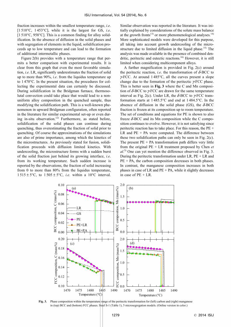
A further magnification is provided in Fig. 2(c) aroundthe peritectic reaction, i.e. the transformation of δ-BCC toγ-FCC. At around 1 485°C, all the curves present a slopechange due to the formation of the peritectic γ-FCC phase.This is better seen in Fig. 3 where the C and Mn composi-tion of δ-BCC to γ-FCC are drawn for the same temperatureinterval as Fig. 2(c). Under LR, the δ-BCC to γ-FCC trans-formation starts at 1 485.5°C and end at 1 484.5°C. In theabsence of diffusion in the solid phase (GS), the δ-BCCfraction is frozen at its composition up to room temperature.The set of conditions and equations for PE is shown to alsofreeze δ-BCC and its Mn composition while the C compo-sition continues to evolve. However, it is not satisfying sinceperitectic reaction has to take place. For this reason, the PE +LR and PE + PA were computed. The difference betweenthese two solidification paths can only be seen in Fig. 2(c).The present PE + PA transformation path differs very littlefrom the original PE + LR treatment proposed by Chen etal.5) One can yet mention the difference observed in Fig. 3.During the peritectic transformation under LR, PE + LR andPE + PA, the carbon composition decreases in both phases.In contrast, the manganese composition increases in bothphases in case of LR and PE + PA, while it slightly decreasesin case of PE + LR.
Fig. 3. Phase composition within the temperature range of the peritectic transformation for (left) carbon and (right) manganesein (top) BCC and (bottom) FCC phases. Steel S-1 (Table 1), 5 microsegregation models. (Online version in color.)

© 2014 ISIJ 1280
ISIJ International, Vol. 54 (2014), No. 6
4.2. Transformation Path for S-2In order to better analyze the PE + LR and PE + PA
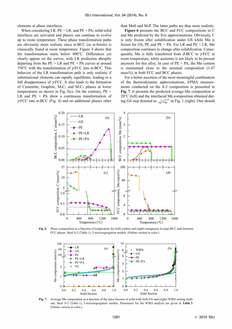
approximations, experimental and numerical studies wereconducted on alloy composition S-2 given in Table 1.Figure 4 shows the evolutions of BCC and FCC fractionswhen cooling the alloy from the liquid state up to room tem-perature. These evolutions are also given for intermetallicsMnS, M3P, and other phases in Fig. 5. Similar observationsare found as for alloy S-1 upon primary δ-BCC solidifica-tion and the δ-BCC to γ-FCC peritectic transformation forthe five approximations considered, i.e. δ-BCC is frozenbelow the peritectic temperature under GS and PE. Note inFigs. 5(a) and 5(b) the large differences found between theprecipitation temperatures of the MnS and M3P phases,respectively. The GS approximation predicts the lowest pre-cipitation temperatures for these phases. It also reveals pre-cipitation of Cementite and Graphite from the melt ataround 950°C (Fig. 5(c)). Such large solidification intervalis not likely to be achieved and this is clearly a limitationof the GS approximation. The PEs approximations also pre-dict formation of the MnS and M3P phases slightly above1 000°C. At lower temperature, all phase fractions arelocked under GS and PE. As stated before, this is coherentwith solute mass balance analysis of frozen substitutional
Fig. 4. Mass fraction of phases as a function of temperature for(top) δ-BCC and (bottom) γ-FCC. Steel S-2 (Table 1),5 microsegregation models. (Online version in color.)
Fig. 5. Mass fraction of phases as a function of temperature for (top) MnS, (middle) M3P and (bottom) other intermetal-lics. Steel S-2 (Table 1), 5 microsegregation models. (Online version in color.)
ISIJ International, Vol. 54 (2014), No. 6
1281 © 2014 ISIJ
elements at phase interfaces.When considering LR, PE + LR, and PE + PA, solid-solid
interfaces are activated and phases can continue to evolveup to room temperature. These phase transformation pathsare obviously more realistic since α-BCC (or α-ferrite) isclassically found at room temperature. Figure 4 shows thatthe transformation starts below 800°C. Differences yetclearly appear on the curves, with LR prediction abruptlydeparting from the PE + LR and PE + PA curves at around750°C with the transformation of γ-FCC into α-BCC. Thisbehavior of the LR transformation path is only realistic ifsubstitutional elements can rapidly equilibrate, leading to afull disappearance of γ-FCC. It also leads to the formationof Cementite, Graphite, M5C2 and M7C3 phases at lowertemperatures as shown in Fig. 5(c). On the contrary, PE +LR and PE + PA show a continuous transformation ofγ-FCC into α-BCC (Fig. 4) and no additional phases other
than MnS and M3P. The latter paths are thus more realistic.Figure 6 presents the BCC and FCC compositions in C
and Mn predicted by the five approximations. Obviously, Cis only frozen after solidification under GS while Mn isfrozen for GS, PE and PE + PA. For LR and PE + LR, Mncomposition continues to change after solidification. Conse-quently, Mn is fully transferred from δ-BCC to γ-FCC atroom temperature, while austenite is not likely to be presentanymore for this alloy. In case of PE + PA, the Mn contentis maintained close to the nominal composition (1.47mass%) in both FCC and BCC phases.
For a better assertion of the most meaningful combinationof the thermodynamic approximations, EPMA measure-ments conducted on the S-2 composition is presented inFig. 7. It presents the predicted average Mn composition at20°C (left) and the interfacial Mn composition obtained dur-ing GS step denoted as in Fig. 1 (right). One shouldEQ
kMnpx j ≠1
Fig. 6. Phase composition as a function of temperature for (left) carbon and (right) manganese in (top) BCC and (bottom)FCC phases. Steel S-2 (Table 1), 5 microsegregation models. (Online version in color.)
Fig. 7. Average Mn composition as a function of the mass fraction of solid with (left) FG and (right) WIRS sorting meth-ods. Steel S-2 (Table 1), 5 microsegregation models. Parameters for the WIRS analysis are given in Table 3.(Online version in color.)

© 2014 ISIJ 1282
ISIJ International, Vol. 54 (2014), No. 6
notice that the sample analyzed contains MnS, thus explain-ing the rapid increase of Mn content in the composition pro-files for solid fraction above 0.95. The GS, PE and PE + PAapproximations are found to provide better agreement withthe measurements, using both the FG and WIRS sortingmethods, i.e. when Mn diffusion is frozen. A clear changein the composition profile is yet predicted under GS, PE andPE + PA, when the solid fraction reaches around 0.65. It isdue to the δ-BCC to γ-FCC transformation. According toprevious considerations, the overall best agreement is thusfound for the combination of PE + PA approximations.
5. Conclusion
(1) Combination of the partial- and para- equilibrium(PE + PA) thermodynamic approximations is proposed forthe study of phase transformations in steels, from the liquidstate to room temperature.
(2) Calculated solidification paths for multi-componentalloys are discussed with respect to the peritectic transfor-mation. It is found that, in case of PE + PA, the solidificationpath does not differ significantly from the lever rule (LR)and from the combination of the partial equilibrium pluslever rule (PE + LR) approximations.
(3) Differences with experimental results are discussedbased on analyses of a sample processed by Bridgman solid-ification, showing the need for more accurate experimental
results and removal of several modeling hypotheses(absence of microstructures kinetics and no treatment oflimited diffusion in all phases).
(4) Regarding the solid state phase transformations, PE +PA is found to provide the most realistic composition profileof substitutional elements and evolution of the phase frac-tions. PE + PA is therefore recommended as the standard setof thermodynamic approximations to be used for the studyof phase transformations in multicomponent steels.
AcknowledgmentsThis work has been supported by Nippon Steel &
Sumitomo Metal Corporation (Tokyo, Japan) in a collabo-ration project with ArcelorMittal Maizières Research(Maizières-lès-Metz, France).
REFERENCES
1) G. H. Gulliver: J. Inst. Met., 9 (1913), 120.2) E. Scheil: Z. Metallkd., 34 (1942), 70.3) Q. Chen and B. Sundman: Mater. Trans., 43 (2002), 551.4) H. Zhang, K. Nakajima, C. A. Gandin and J. He: ISIJ Int., 53 (2013),
493.5) Q. Chen, A. Engstrom, X.-G. Lu and B. Sundman: MCWASP-XI, ed.
by Ch.-A. Gandin and M. Bellet, TMS, Warrendale, PA, (2006), 529.6) Thermo-Calc TCCS Mnuals, Thermo-Calc Sftware AB, Stockholm,
Sweden, (2013).7) P. Shi: TCS steels/Fe-alloys Dtabase, V6.0, Thermo-Calc Software
AB, Stockholm, Sweden, (2008).8) M. Hillert: Phase Equilibria, Phase Diagrams and Phase Transforma-
tions, Cambridge University, UK, (1998), 358.9) W. Kurz and D. J. Fisher: Fundamentals of Solidification, Trans Tech
Publications Ltd, Switzerland, (1998), 7.10) J. A. Dantzig and M. Rappaz: Solidification, EPFL Press, Lausanne,
Switzerland, (2009), 17.11) M. Ganesan and P. D. Lee: Mater. Trans. A, 36 (2005), 2191.12) A. Bogno, H. Nguyen-Thi, G. Reinhart, B. Billia and J. Baruchel:
Acta Mater., 61 (2013), 1303.13) J. A. Sarreal and G. J. Abbaschian: Mater. Trans. A, 17 (1986), 2063.14) B. Giovanola and W. Kurz: Mater. Trans. A, 21 (1990), 260.15) C. Y. Wang and C. Beckermann: Mater. Sci. Eng. A, 171 (1993), 199.16) D. Tourret, Ch.-A. Gandin, T. Volkmann and D. M. Herlach: Acta
Mater., 59 (2011), 4665.
Table 3. Data for WIRS (mass%). σ is uncertainty, estimated as thedifference between nominal composition and averagecomposition of EPMA measurements.
Mn S P
Min 0 0 0
σ 0.026 0.004 0.004