Computability of Preference,

Utility, and Demand

by

Marcel K. Richter and Kam-Chau Wong

Discussion Paper No. 298, December 1996

Center for Economic Research Department of Economics University of Minnesota Minneapolis, MN 55455

Computability of Preference, Utility, and Demand

by

Marcel K. Richter

Department of Economics, University of Minnesota, Minnesota MN 55455, U.S.A.

and

Kam-Chau Wong •

Department of Economics, Chinese University of Hong Kong, Shatin, Hong Kongt

Abstract: This paper studies consumer theory from the bounded rationality ap­proach proposed in Richter and Wong (1996a), with a "uniformity principle" con­straining the magnitudes (prices, quantities, etc.) and the operations (to perceive, evaluate, choose, communicate, etc.) that agents can use. In particular, we operate in a computability framework, where commodity quantities, prices, consumer pref­erences, utility functions, and demand functions are computable by finite algorithms (Richter and Wong (1996a)).

We obtain a computable utility representation theorem. We prove an existence theorem for computable maximizers of quasiconcave computable utility functions (preferences), and prove the computability of the demand functions generated by such functions (preferences). We also provide a revealed preference characterization of computable rationality for the finite case. Beyond consumer theory, the results have applications in general equilibrium theory (Richter and Wong (1996a)).

JEL Classification: Dll, C63

Keywords: Bounded rationality, Consumer theory, Convex Optimization, Re­vealed Preference Analysis, Recursive Analysis, Utility Represen­tation

-Financial support from the Chinese University of Hong Kong is gratefully acknowledged. I thank the Department of Economics, University of Minnesota for the hospitality and support provided to me during the winter and spring of 1996.

tE-mail: kamchauwongOcuhk.hk; phone: (852) 2609-7053; fax: (852) 2603-5805.

1. INTRODUCTION

One approach to bounded rationality limits the operations that agents can per­form to a class of "simple" decision rules. As noted in Richter and Wong (1996b) it is natural to limit magnitudes, as well as operations, to simple classes. In this paper, we examine agents whose operations and magnitudes are both limited by the agents' abilities in performing computations: we impose a computability bound on their rationality. The results are of interest not only for consumer theory, but have applications in the study of general equilibrium in a boundedly rational context (Richter and Wong (1996a)).

In the classical approach, agents can perform arbitrarily complicated calculations on arbitrarily complicated magnitudes. Such extreme calculating abilities have been recognized as unrealistic in many situations (cf. Simon (1959, 1978)). In Richter and Wong (1996a), we also pointed out the unrealistic nature of perceiving and communicating arbitrary magnitudes. To incorporate "realistic" limitations on calculation and communication, we first ask what operations, or calculations, human beings can perform. A widely accepted view is that routine human calculating abilities are limited to those of the ideal computing machines known as Turing machines. (Cf. Turing (1950)).

Even within the bounds of Turing computability, there are interesting subclasses (polynomial-time Turing machines, finite automata, etc.; cf. Davis (1983)). In this paper, however, we examine the consequences of assuming our agents' calculating abilities coincide with those of Turing machines~ (This is known as Church's Thesis (cf. Church (1935).)

We will apply this Turing computability notion to magnitudes as well as to operations. In particular, our agents can only use "computable" numbers (as prices, commodity quantities, utility parameters, etc.) - i.e. those reals whose decimal (hence digital, etc.) representations can be computed by Turing machines. One realistic consequence is this: Since each Turing machine can be represented by a single integer (Godel number), each computable real can be represented by an integer code. Thus agents can communicate prices and quantities without needing an uncountable vocabulary.

Similarly, binary preference rankings of our agents are determined by Turing machines. Indeed, all functions we consider will also be "computable."

Beyond bounded rationality, results in the present context can have useful im­plications for applied economics - in particular, for computational economics. For example, if an economist seeks an algorithm to solve a constrained maximization problem, he needs to know whether such an algorithm exists. By our definition

2

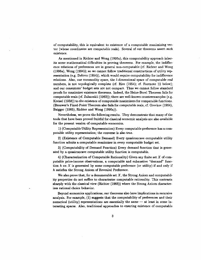
of computability, this is equivalent to existence of a computable maximizing vec­tor (whose coordinates are computable reals). Several of our theorems assert such existence.

As mentioned in Richter and Wong (1996a), this computability approach inher­its some mathematical difficulties in proving theorems. For example, the indiffer­ence relations of preferences are in general non-computable (cf. Richter and Wong (1996a), Wong (1994)); so we cannot follow traditional constructions of utility rep­resentation (e.g. Debreu (1954)), which would require computability for indifference relations. Also, our commodity space, the I-dimensional space of computable real numbers, is not topologically complete (cf. Rice (1954); cf. Footnote 12 below); and our consumers' budget sets are not compact. Thus we cannot follow standard proofs for maximizer existence theorems. Indeed, the Heine-Borel Theorem fails for computable reals (cf. Zalsavskii (1962)); there are well-known counterexamples (e.g. Kreisel (1958)) to the existence of computable maximizers for computable functions. (Brouwer's Fixed-Point Theorem also fails for computable reals, cf. Orevkov (1964), Baigger (1985), Richter and Wong (1996a)).

Nevertheless, we prove the following results. They demonstrate that many of the tools that have been proved fruitful for classical economic analysis are also available for the present version of computable economics.

1) (Computable Utility Representation) Every computable preference has a com­putable utility representation; the converse is also true.

2) (Existence of Computable Demand) Every quasiconcave computable utility function admits a computable maximizer in every computable budget set.

3) (Computability of Demand Function) Every demand function that is gener­ated by a quasiconcave computable utility function is computable.

4) (Characterization of Computable Rationality) Given any finite set X of com­putable price-income observations, a computable and exhaustive "demand" func­tion h on X is generated by some computable preference (or utility) if and only if h satisfies the Strong Axiom of Revealed Preference.

We also prove that, for a denumerable set X, the Strong Axiom and computabil­ity properties do not suffice to characterize computable rationality. This contrasts sharply with the classical view (Richter (1966)) where the Strong Axiom character­izes rational choice behavior.

Beyond economics applications, our theorems also have implications in recursive analysis. For example, (1) suggests that the computability of preferences and their numerical (utility) representations are essentially the same - at least in some in­teresting spaces. Also, traditional approaches to ensuring existence of computable

3

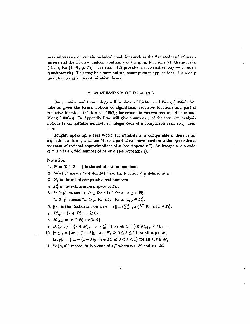
maximizers rely on certain technical conditions such as the "isolatedness" of maxi­mizers and the effective uniform continuity of the given functions (cf. Grzegorczyk (1955), Ko (1991, p. 75). Our result (2) provides an alternative way - through quasiconcavity. This may be a more natural assumption in applications; it is widely used, for example, in optimization theory.

2. STATEMENT OF RESULTS

Our notation and terminology will be those of Richter and Wong (1996a). We take as given the formal notions of algorithms: recursive functions and partial recursive functions (cf. Kleene (1952); for economic motivations, see Richter and Wong (1996a)). In Appendix I we will give a summary of the recursive analysis notions (a computable number, an integer code of a computable real, etc.) used here.

Roughly speaking, a real vector (or number) z is computable if there is an algorithm, a Turing machine M, or a partial recursive function ¢ that generates a sequence of rational approximations of z (see Appendix I). An integer n is a code of z if n is a Gooel number of M or ¢ (see Appendix I).

Notation.

1. IN = {O, 1,2, ... } is the set of natural numbers.

2. "¢(z).J.." means "z E dom(¢)," i.e. the function ¢ is defined at z.

3. IRe is the set of computable real numbers.

4. IR~ is the I-dimensional space of IRe.

5. "z ~ Y" means "Zi ~ Yi for all i," for all z, Y E IR~,

"z »y" means "Zi > Yi for all z'" for all z, Y E IR~.

6. II· II is the Euclidean norm, i.e. IIzil = (E~=l Zi)1/2 for all z E IR~. 7. IR~+ = {z E ~ : Zi ~ OJ.

8. ~++ = {z E IR~ : z» OJ.

9. Be(P, w) = {z E ~+ : p. z ~ w} for all (p, w) E IR'e++ x IRe++.

10. [z, Y]e = {AZ + (1- A)Y : A E IRe & 0 ~ A ~ I} for all z, Y E IR~

(z, Y)e = {AZ + (1 - A)Y : A EIRe & 0 < A < I} for all z, Y E IR~.

11. "A(n,z)" means "n is a code of z," where n E IN and z E IR~.

4

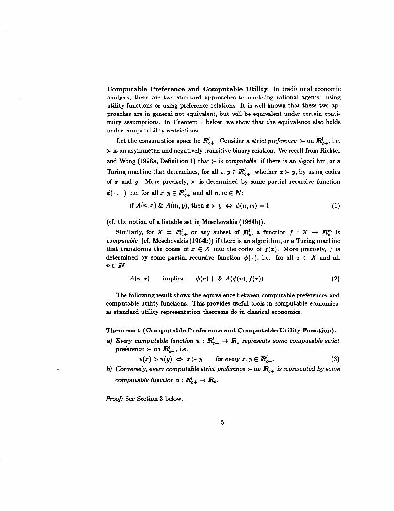
Computable Preference and Computable Utility. In traditional economic analysis, there are two standard approaches to modeling rational agents: using utility functions or using preference relations. It is well-known that these two ap­proaches are in general not equivalent, but will be equivalent under certain conti­nuity assumptions. In Theorem 1 below, we show that the equivalence also holds under computability restrictions.

Let the consumption space be IR~+. Consider a strict preference ~ on IR~+, i.e.

~ is an asymmetric and negatively transitive binary relation. We recall from Richter

and Wong (1996a, Definition 1) that ~ is computable if there is an algorithm, or a

Turing machine that determines, for all x, y E IR~+, whether x ~ y, by using codes

of x and y. More precisely, ~ is determined by some partial recursive function

¢( " .), i.e. for all x, y E IR~+ and all n, mE IN:

if A(n, x) & A(m, y), then x ~ y ¢:> ¢(n, m) = 1, (1)

(cf. the notion of a listable set in Moschovakis (1964b)).

Similarly, for X = IR~+ or any subset of IR~, a function f : X ~ IRr;' is computable (cf. Moschovakis (1964b)) if there is an algorithm, or a Turing machine that transforms the codes of x E X into the codes of f(x). More precisely, f is determined by some partial recursive function t/J(.), i.e. for all x E X and all n E IN:

A(n, x) implies t/J(n) r & A(t/J(n),f(x)) (2)

The following result shows the equivalence between computable preferences and computable utility functions. This provides useful tools in computable economics, as standard utility representation theorems do in classical economics.

Theorem 1 (Computable Preference and Computable Utility Function).

a) Every computable function u : IR~+ ~ IRe represents some computable strict preference ~ on IR~+, i.e.

u(x) > u(y) ¢:> x ~ y for every x, y E ~+. (3)

b) Conversely, every computable strict preference ~ on IR~+ is represented by some

computable function u : Rc+ ~ IRe.

Proof: See Section 3 below.

5

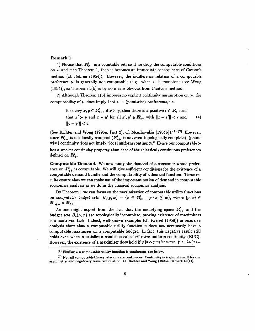
Remark 1.

1) Notice that lR~+ is a countable set; so if we drop the computable conditions on ~ and u in Theorem 1, then it becomes an immediate consequence of Cantor's

method (cf. Debreu (1954)). However, the indifference relation of a computable preference ~ is generally non-computable (e.g. when ~ is monotone (see Wong

(1994)); so Theorem l(b) is by no means obvious from Cantor's method.

2) Although Theorem l(b) imposes no explicit continuity assumption on ~, the

computability of ~ does imply that ~ is (pointwise) continuous, i.e.

for every z, y E lR~+, if z ~ y, then there is a positive f E lRe such

that z' ~ y and z ~ y' for all z', y' E lR~+ with liz - z'lI < f and (4)

lIy - y'li < f.

(See Richter and Wong (1996a, Fact 2); cf. Moschovakis (1964b)).(1) (2) However, since lR~+ is not locally compact (lR~+ is not even topologically complete), (point­wise) continuity does not imply "local uniform continuity." Hence our computable ~

has a weaker continuity property than that of the (classical) continuous preferences defined on lR~.

Computable Demand. We now study the demand of a consumer whose prefer­ence on lR~+ is computable. We will give sufficient conditions for the existence of a computable demand bundle and the computability of a demand function. These re­sults ensure that we can make use of the important notion of demand in computable economics analysis as we do in the classical economics analysis.

By Theorem 1 we can focus on the maximization of computable utility functions on computable budget sets Be (p, w) = {z E ~+ : p . z ~ w}, where (p, w) E

lR~++ x lRe++.

As one might expect from the fact that the underlying space lR~+ and the budget sets Be(P, w) are topologically incomplete, proving existence of maximizers is a nontrivial task. Indeed, well-known examples (cf. Kreisel (1958)) in recursive analysis show that a computable utility function u does not necessarily have a computable maximizer on a computable budget. In fact, this negative result still holds even when u satisfies a condition called effective uniform continuity (EUC). However, the existence of a maximizer does hold if u is c-quasiconcave (i.e. AU( z) +

(1) Similarly, a computable utility function is continuous; see below.

(2) Not all computable binary relations are continuous. Continuity is a special result for our asymmetric and negatively transitive relation. Cf. Richter and Wong (l996a, Remark 13(4)).

6

(1- ..\)u(y) ~ min{u(x), u(y)} for all x, y E lR~+ and all ..\ E [0, l]e = {..\ E lRe : 0 ~ ..\ ~ I}) and satisfies EVC (see Wong (1996)). In Theorem 2, we go further, and show that we can drop EVC, retaining only the economically natural quasiconcavity condition.

Theorem 2 (Existence of a Computable Demand Bundle). Let u: lR~+ -+ lRe be computable and c-quasiconcave. Then for every (p, w) E lR~++ X lRe++, the function u admits a computable maximizer on Be(P, w).

Proof. See Section 4.

Remark 2.

1) By Theorem 1, Theorem 2 can be rephrased in terms of computable prefer­ences; see Richter and Wong (1996a, Theorem 2).

2) Theorem 2 shows the possibility of using algorithms in maximizing quasi­concave objective functions. That is because by our definition, computability of a maximizer x is equivalent to existence of an algorithm that calculates digital approximations of x to any desired degree of accuracy within a known time.

3) As in Remark 1(2), a computable function u : lR~+ -+ lRe is (pointwise) continuous, i.e.

for every x E lR~+ and every positive f E lRe, there is a positive 6 E.IRe such that lu(x)-u(y)1 < 6 for all y E lR~+ with IIx-yil < 6

(5)

(see Moschovakis (19Mb, Theorem 3 and Corollary 4.1); cf. Richter and Wong (1996a, Fact 2)). Hence, although we have dropped EVC as an hypothesis from Theorem 2, we still get some continuity as a conclusion.

Theorem 2 asserts only the existence of computable demand bundles, but not a computable demand function. In Theorem 3, without making any new assumptions, we show the computability of any demand function h : lR~++ x lRe++ -+ lR~+ that is generated by some computable c-quasiconcave utility function u : lR~+ -+ lRe, I.e.

h(p, w) = argmaJe,reBc(p,w)u(x)

for all (p, w) E ~++ x lRe++.

(6)

Theorem 3 (Computability of Demand Function). Let h : lR~++ x lRe++ -+ lR~+ be a demand function generated by some computable and c-quasiconcave func­tion u : ~+ -+.IRe. Then h is computable.

7

Proof: See Section 4 below.

Remark 3.

1) Since the function h : lR~++ x lRe++ -+ lR~+ is computable, it is also contin­uous (Moschovakis (1964b, Theorem 3); cf. Richter and Wong (1996a, Fact 2)).

2) By Theorem 1, Theorem 3 can be rephrased in terms of computable prefer­ences; see Richter and Wong (1996a, Theorem 3).

3) We establish Theorem 3 by using Proposition 1(2), whose proof uses an al­gorithm that finds h(p, w) for any given (p, w) E lR~++ X lRe++. (Cf. Bridges' algorithmic proof (1992) for existence of a demand function in the context of con­structive mathematics (cf. Bishop (1967))).

4) Let u : lR~+ -+ lRe be strictly c-quasiconcave, i.e. u(>.x + (1 - >.)y) > min{u(x), u(y)} for all >. E (O,I)e and all pairs of distinct x, y E lR~+.(3) Clearly strict c-quasiconcavity implies c-quasiconcavity (but not vice versa). Suppose u is also computable. Then by Theorem 2 and the definition of strict c-quasiconcavity, it is clear that u admits a unique computable maximizer on every computable budget set, so u generates a demand function h :' lR~++ x lRe++ -+ lR~+. By Theorem 3 this h is indeed computable.

5) Let u : lR~+ -+ lRe be strictly monotone, i.e. u(x) > u(y) for all x, y E lR~+ with x ~ y and x 1: y.(4) If h : lR~++ x lRe++ -+ ~ is the demand function generated by u, then it is clear that h is exhaustive, i.e. p. h(p) = w for all (p, w) E lR~++ X lRe++.

6) In contrast to classical models, computable demand functions and computable excess demand functions (cf. Remark 9(2,11) in Appendix II) need not satisfy the standard "boundary conditions," even when they are generated by strictly c­quasiconcave and strictly monotone utility functions. (Cf. Footnotes 3 and 4; see Remark 9 in Appendix II.)

Revealed Preference Analysis. Consider a computable consumer whose com­putable utility function u : lR~+ -+ lRe is strictly c-quasiconcave and strictly mono­tone. By Remarks 3(4) and 3(5), the consumer has a computable and exhaustive demand function on lR~++ x lRe++; so for any X £ lR~++ x 1Rc++, the restriction

(3) The strict c-quasiconcavity of u on R~+ does not imply strict quasiconcavity of the

extension of u to all of R~. This is true even when u has a unique continuous extension to R~

(see Appendix II).

(4) As with strict c-quasiconcavity (c!. Footnote 3) the strict monotonicity property fails for continuous extension from R~+ to R~ (c!. Appendix II). .

8

h of his demand is a computable function from X to lR~+ and is exhaustive on X (i.e. p. h(p) = w for all (p, w) E X). Moreover, h clearly satisfies Houthakker's Strong Axiom of Revealed Preference (cf. Richter (1966»: the binary relation S on lR~+ is acyclic (i.e. xSyS··· zSx is impossible), where S is defined by "xSy if x::j: y & x = h(p,w) & y E Be(p,w) for some (p,w) EX."

Thus the computability, exhaustiveness, and Strong Axiom properties are nec­essary for a demand function h : X ~ lR~+ to be the demand of such "classical­rational" computable consumer. The following result, which is a computable ver­sion of Matzkin and Richter (1991, Theorem 1), shows the converse for the finite case. Notice that the utility function U : lR~+ ~ lRe that we obtain in Theorem 4 is strictly c-concave (rather than just c-quasiconcave), i.e. U(AX + (1 - A)Y) > AU(X) + (1 - A)U(y) for all A E (0, l)e and all x, y E lR~+ with x ::j: y.

Theorem 4 (Characterization of Computable Classical-Rationality). Let X be a finite set in lR~++ x lRe++. If h : X ~ lR~+ is computable,(5) exhaustive, and satisfies the Strong Axiom of Revealed Preference, then there is a computable, strictly monotone, and strictly c-concave function U : lR~+ ~ lRe that generates h on X, i.e. (6) holds on X.

Proof: See Section 5 below.

Remark 4. When X is not finite, the Strong Axiom by itself does not necessarily imply existence of a utility generator. To see this, consider the function h defined in Hurwicz and Richter (1971, p. 65). The function h is exhaustive, and satisfies the Strong Axiom. Also it is easily verified that h is computable on lR~++ x lRe++. As in Hurwicz and Richter (p. 66), for the computable point x = (1,0) we can find a computable point y in lR~+ that is revealed worsen than x and find a (not­necessarily-computable) sequence of computable points ao, a1, ... in lR~+ convergent to x and such that each ak is revealed worsen than y. Suppose h is rationalized by a (not-necessarily-computable) utility function u. Then U must satisfy u(x) > u(y) > u(ak), so u cannot be continuous at x, hence u cannot be computable (cf. (5».

(5) Notice that when X ~ R~++ X Rc++ is finite, then every function h : X -+ R~+ is computable, since h is the restriction of some (computable) function 9 = (91,92) whose components 9i are polynomials with computable coefficients.

9

3. PROOF OF THEOREM 1

Proof of Theorem l(a). Let u : lR~+ -t lRe be computable. Then it is clear that (3) defines a strict preference relation ~ on lR~+.

To show the computability for ~, we pick a partial recursive function ¢( . ) that

determines u. We also pick a partial recursive function 'I/J( . , • ) that determines the computable relation> (cf. Richter and Wong (1996a, Footnote 14)). We now show that ~ is determined by the partial recursive function !p(n, n') = 'I/J(¢(n) , ¢(n')).

For any x,x' E lR~+ and any n,n' E IN with A(n,x) and A(n',x'), we have: A(¢(n), u(x)) and A(¢(n'), u(x')); so u(x) > u(x') ¢::> 'I/J(¢(n) , ¢(n')) = 1, and hence x ~ x' ¢::> !p(n, n') = 1. Q.E.D.

In our proof of Theorem 1 (b), we will derive a computable utility representation u for an arbitrary computable preference ~. We will begin with a common approach

(cf. Debreu (1954)) to construction of utility representations: we start by defining a function on a countable ~-dense subset, and then take limits. But to obtain the

computability of u, we need to ensure the computability of the construction process. Therefore our construction cannot employ the weakly preferred or indifference rela­tions of~, because they are generally noncomputable. So we modify the common

approach and use only the strictly preferred relation.

In order to make use of the computability of ~ in a "deterministic" (recursive)

way, we will use the following observation: Let >- be a computable strict preference

on lR~+. Then ~ is determined by some partial recursive function ¢ as given in (1).

By the Normal Form Theorem (cited in Fact 1(1), page 26) we can pick a recursive function(6) lit : IN x IN x IN -t IN such that for all n, n' E IN: ¢(n, n') = 1 ¢::>

(3m E IN)[lIt(m, n, n') = 0]; hence by (1), for all x, x' E ~+ and all n, n' E IN:

ifA(n, x) & A(n',x'),then: x~x' ¢::> (3mEIN)[lIt(m,n,n') =0]. (7)

(Intuitively, lIt(m, n, n') can be interperted as "the algorithm lit takes m steps to determine x ~ x'.")

Also, we will take as given the notion of a recursive sequence of rational vectors (cf. Appendix I).

(6) Recall that by definition a recursive function is total, thus 'W'{m, n, n'} -l. for all m, n, n' E N, i.e. dom{'W'} = N x N x N.

10

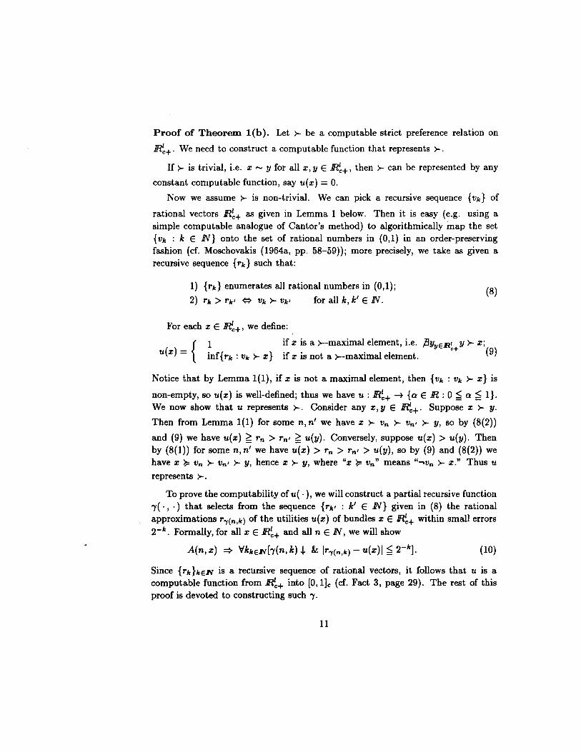
Proof of Theorem l(b). Let >- be a computable strict preference relation on

IR~+. We need to construct a computable function that represents >-.

If >- is trivial, i.e. x"'" y for all x, y E IR~+, then >- can be represented by any

constant computable function, say u(x) = o. Now we assume >- is non-trivial. We can pick a recursive sequence {Vk} of

rational vectors IR~+ as given in Lemma 1 below. Then it is easy (e.g. using a simple computable analogue of Cantor's method) to algorithmically map the set {Vk : k E .DV} onto the set of rational numbers in (0,1) in an order-preserving fashion (cf. Moschovakis (1964a, pp. 58-59)); more precisely, we take as given a recursive sequence {rk} such that:

1) {rk} enumerates all rational numbers in (0,1);

2) rk > rk' ¢:> Vk >- Vk' for all k, k' E .DV. (8)

For each x E IR~+, we define:

u(x) = { 1 if x is a >--maximal element, i.e. !JYYER' Y >- x;

inf{rk : Vk >- x} if x is not a >--maximal element. c+ (9)

Notice that by Lemma 1(1), if x is not a maximal element, then {Vk : Vk >- x} is

non-empty, so u(x) is well-defined; thus we have u : IR~+ -+ {a E IR : 0 ~ a ~ I}. We now show that u represents >-. Consider any x, Y E IR~+. Suppose x >- y.

Then from Lemma 1(1) for some n, n' we have x >- Vn >- Vn , >- y, so by (8(2))

and (9) we have u(x) ~ rn > rn , ~ u(y). Conversely, suppose u(x) > u(y). Then by (8(1» for some n, n' we have u(x) > rn > rn , > u(y), so by (9) and (8(2» we have x ~ Vn >- Vn ' >- y, hence x >- y, where "x ~ vn " means "-,vn >- x." Thus u

represents >-.

To prove the computability of u( . ), we will construct a partial recursive function 'Y( ., .) that selects from the sequence {rk' : k' E .DV} given in (8) the rational approximations r-y(n,k) of the utilities u(x) of bundles x E IR~+ within small errors 2-k . Formally, for all x E IR~+ and all n E .DV, we will show

A(n, x) => 'v'kkEJV[,},(n, k) -I- & Ir-y(n,k) - u(x)1 ~ 2-k]. (10)

Since {rk}kEJV is a recursive sequence of rational vectors, it follows that u is a computable function from ~+ into [O,I]c (cf. Fact 3, page 29). The rest of this proof is devoted to constructing such 'Y.

11

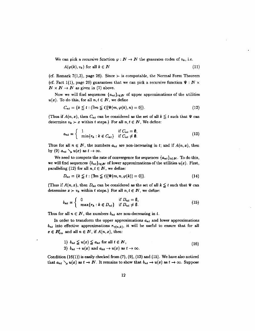
We can pick a recursive function cp : IN ~ IN the generates codes of Vk, i.e.

A(cp(k), Vk) for all k E IN (11)

(cf. Remark 7(1,3), page 26). Since >- is computable, the Normal Form Theorem

(cf. Fact 1(1), page 26) guarantees that we can pick a recursive function W : IN x IN x IN ~ IN as given in (7) above.

Now we will find sequences {anthelV of upper approximations of the utilities u(z). To do this, for all n, t E IN, we define

Cnt = {k ;£ t : (3m ;£ t)[\II(m, cp(k), n) = OJ}. (12)

(Thus if A(n, z), then Cnt can be considered as the set of all k ;£ t such that W can determine Vk >- z within t steps.) For all n, t E IN, We define:

{I if Cnt = 0,

ant = mini rk : k E Cnd if C nt =F 0. (13)

Thus for all n E IN, the numbers ant are non-increasing in t; and if A(n,z), then by (9) ant'\, u(z) as t ~ 00. .

We need to compute the rate of convergence for sequences {ant helV. To do this, we will find sequences {bnthelV oflower approximations of the utilities u(z). First, paralleling (12) for all n,t E IN, we define:

Dnt = {k ;£ t : (3m ;£ t)[W(m, n, <p(k)) = OJ}. (14)

(Thus if A(n, z), then Dnt can be considered as the set of all k ;£ t such that \II can determine z >- Vk within t steps.) For all n, t E IN, we define:

b _ { 0 if Dnt = 0, nt - max{rk : k E D nt } if Dnt =F 0. (15)

Thus for all n E IN, the numbers bnt are non-decreasing in t.

In order to transform the upper approximations ant and lower approximations bnt into effective approximations r.,(n,k), it will be useful to ensure that for all

z E R~+ and all n E IN, if A(n,z), then:

1) bnt ;£ u(z) ;£ ant for all t E IN, (16) 2) bnt ~ u(z) and ant ~ u(z) as t ~ 00.

Condition (16(1)) is easily checked from (7), (9), (13) and (15). We have also noticed that ant'\, u(z) as t ~ IN. It remains to show that bnt ~ u(z) as t ~ 00. Suppose

12

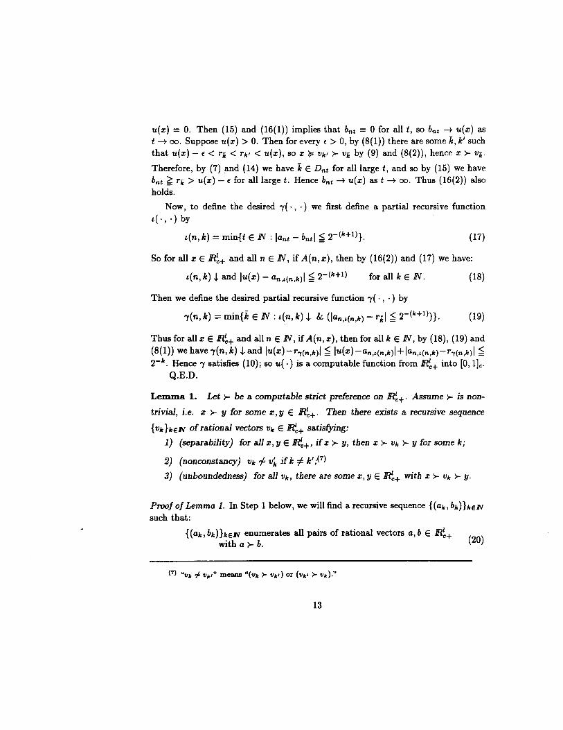
u(x) = O. Then (15) and (16(1)) implies that bnt = 0 for all t, so bnt -+ u(x) as

t -+ 00. Suppose u(x) > O. Then for every { > 0, by (8(1)) there are some k, k' such that u(x) - { < riC < rk' < u(x), so x ~ Vk' >- ViC by (9) and (8(2)), hence x >- ViC·

Therefore, by (7) and (14) we have k E Dnt for all large t, and so by (15) we have bnt ~ riC > u(x) - { for all large t. Hence bnt -+ u(x) as t -+ 00. Thus (16(2)) also holds.

Now, to define the desired -y( ., .) we first define a partial recursive function t( ., . ) by

t(n, k) = min{t E lN : lant - bntl ~ 2-(k+1)}. (17)

So for all x E 1R~+ and all n E lN, if A(n, x), then by (16(2)) and (17) we have:

t(n, k) .J.. and lu(x) - an,£(n,k)1 ~ 2-(k+1) for all k E IN. (18)

Then we define the desired partial recursive function -y( ., .) by

-y(n, k) = min{k E lN : t(n, k).J.. & (Ian,£(n,k) - rkl ~ 2-(k+l))}. (19)

Thus for all x E 1R~+ and all n E lN, if A(n, x), then for all k E lN, by (18), (19) and (8(1)) we have -y(n, k) .J.. and lu(x)-r-y(n,k)1 ~ lu(x)-an,£(n,k)I+lan,£(n,k)-r-y(n,k)1 ~ 2-k • Hence -y satisfies (10); so u( . ) is a computable function from 1R~+ into [0, IJc.

Q.E.D.

Lemma 1. Let >- be a computable strict preference on 1R~+. Assume >- is non­

trivial, i.e. x >- y for some x, y E 1R~+. Then there exists a recursive sequence

{vkheJV of rational vectors Vk E 1R~+ satisfying:

1) (separability) for all x, y E 1R~+, if x >- y, then x >- Vk >- y for some k;

2) (nonconstancy) Vk f v~ if k =1= k';(7)

3) (unboundedness) for all Vk, there are some x, y E 1R~+ with x>- Vk >- y.

Proof of Lemma 1. In Step 1 below, we will find a recursive sequence {(ak, bk)he1V such that:

{(ak, bk)heJV enumerates all pairs of rational vectors a, b E 1R~+ with a >- b. (20)

13

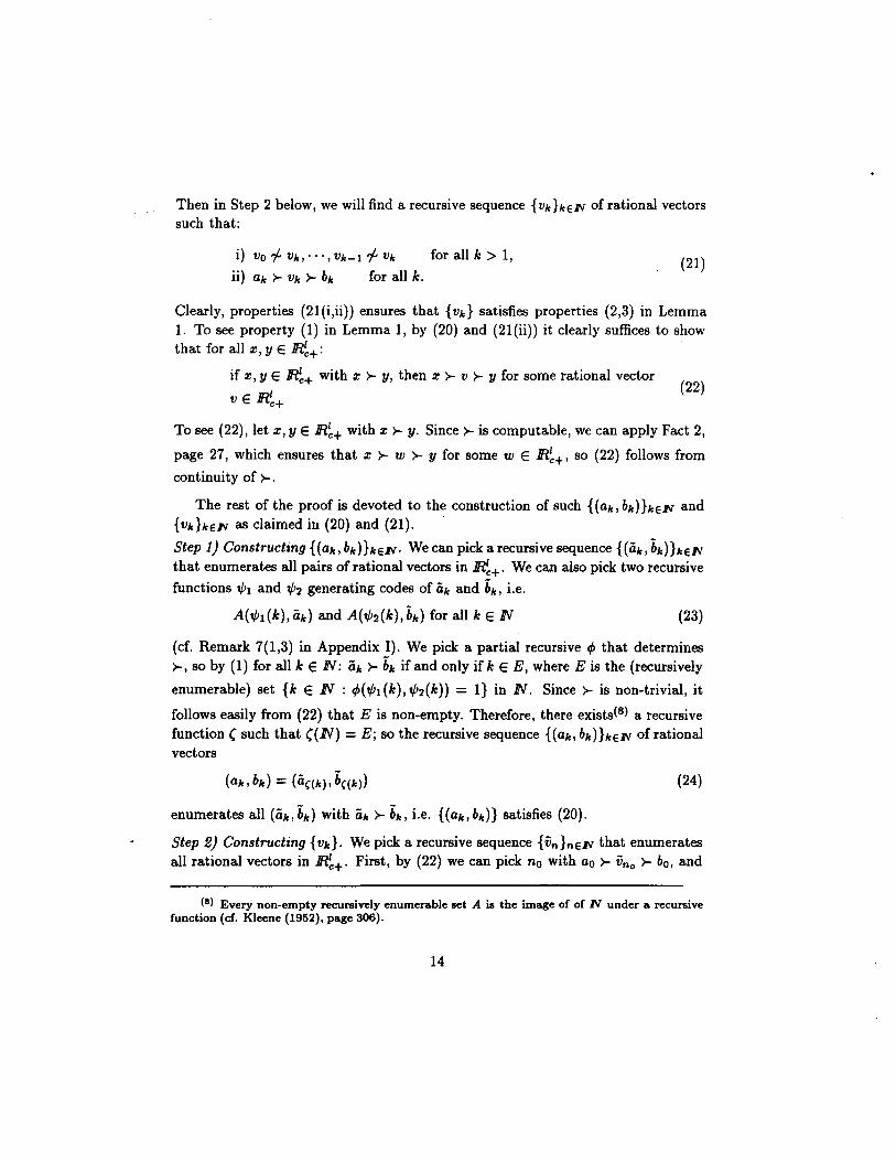
Then in Step 2 below, we will find a recursive sequence {Vie hEN of rational vectors such that:

i) Vo -f Vie,···, VIe-1 -f Vie for all k > 1,

ii) ale )-- Vie )-- ble for all k. (21)

Clearly, properties (21 (i,ii)) ensures that {Vie} satisfies properties (2,3) in Lemma 1. To see property (1) in Lemma 1, by (20) and (21(ii)) it clearly suffices to show that for all x, y E lR~+:

if x, y E lR~+ with x )-- y, then x )-- V )-- Y for some rational vector

V E lR~+ (22)

To see (22), let x, y E lR~+ with x )-- y. Since )-- is computable, we can apply Fact 2,

page 27, which ensures that x )-- w )-- y for some w E lR~+, so (22) follows from

continuity of )--.

The rest of the proof is devoted to the construction of such {(ale, ble)hEN and {VlehElV as claimed in (20) and (21). .

Step 1) Constructing {(a/c, ble)hElV. We can pick a recursive sequence {(ale, hle)hElV that enumerates all pairs of rational vectors in lR~+. We can also pick two recursive

functions tPI and tP2 generating codes of ale and hie, i.e.

(23)

(cf. Remark 7(1,3) in Appendix I). We pick a partial recursive ¢ that determines h so by (1) for all k E IN: ale )-- hie if and only if k E E, where E is the (recursively

enumerable) set {k E IN : ¢(tPI(k),tP2(k)) = I} in IN. Since)-- is non-trivial, it

follows easily from (22) that E is non-empty. Therefore, there exists(8) a recursive function ( such that ((IN) = E; so the recursive sequence {(ale, ble)hElV ofrational vectors

(a/c,ble ) = (a(Ie),h(Ie») (24)

enumerates all (ale, hie) with ale )-- hie, i.e. {(ale,ble)} satisfies (20).

Step 2) Constructing {Vie}. We pick a recursive sequence {tin}nElV that enumerates all rational vectors in lR~+. First, by (22) we can pick no with ao )-- tino )-- bo, and

(8) Every non-empty recursively enumerable set A is the image of of N under a recursive function (d. Kleene (1952), page 306).

14

set e(O) = no· Given any e(O), e(I),···, e(k), by (22) there is some (indeed many) n satisfying:

(25)

So we can pick such n and set e(k + 1) = n. Therefore, the the rational vectors Vk = Ve(k) form a sequence {vkheJV satisfying (21).

To obtain the recursiveness of {Vk}, we need to ensure that the function e ( . ) is recursive. We can obtain this by using a recursive function W given as in (7), codes 1P1«((k)) of ak, codes tP2«((k)) of bk (see (23)), and codes of vn . For example, we pick a recursive function cp that generates codes of vn i.e.

for all n E IN. (26)

Then we set e(O) = no as above. We continue as follows. At any k-th stage, we are given (0),··· ,(k). Notice that for all n E lN, by (7), (22),(23), and (26) n satisfies (25) if and only if there exists some m E lN such that

pt(m, cp(n), cp(e(O)),··· , "<p(k)) & Pk(m, cp(n)), (27)

where these recursive predicates are defined by

Pt (m, cp(e(O)), ... , cp(e(k)), cp(n))

= Af=1[(3m' ~ m)(w(m', cp(e(i)), cp(n)) = 0)

V (3m' ~ m)(w(m', cp(n), cp(e(i))) = 0)] (28)

Pk(m, cp(n)) = [(3m' ~ m)(w(m', tPl«((k + 1)), cp(n)) = 0)

& (3m' ~ m)(w(m', cp(n), tP2«((k + 1))) = 0)],

Then we can define e(k + 1) = min{n ~ M : (3m ~ M)[(m, n) satisfies (27)]), where M = min{M E lN : (3n, m ~ M)[(m, n) satisfies (27)]). It is clear that e( . ) is recursive and for all k E lN, (25) holds with n = e(k+l), as we desire. Q.E.D.

4. PROOF OF THEOREMS 2 AND 3

We take as given the notions of a recursive sequence of rational vectors and a computable sequence of computable vectors (cf. Appendix I).

To prove Theorems 2 and 3, we will make use of Proposition 1 below, which asserts, under the (CC) assumption below, the existence of computable maximizers, and asserts existence of an algorithm for finding unique computable maximizers.

15

Comment 1. To motivate the (CC) assumption, consider the maximization of a given computable function u. To find a computable maximizer, a standard approach is this: 1) First find ok-best elements Xk, i.e. supu - U(Xk) ~ Ok, where Ok '\t O. 2) Then ensure that the Xk converge to some x. To obtain the computability of x, by recursive completeness (cf. Remark 7(2), page 26) it suffices to ensure the com­putability for both the Xk sequence and its rate of convergence. If u is computable, it is easy to obtain the computability of such Xk sequence. If u also satisfies an effective uniform continuity property (EUC), then it is easy to approximate effec­tively the sets 'Pa. of ok-best elements (cf. Pour-EI and Richards (1989, p. 40-41) and Ko (1991, p. 73 (proof of Theorem 3.1)), and hence to approximate effectively their radii. Notice that Xk ' E 'Pa•, ~ 'Pa. for all k, k' with k' ~ k. Therefore, if we further know that the radii of'Pa• '\t 0,(9) then (cf. Pour-EI and Richard (1989, p. 20, Corollary 2a)) we can compute the rate of convergence of the radii of 'Pa .,

and also the rate of convergence of the vectors Xk (cf. Grzegorczyk (1955)).

Remark 5. In the following Proposition 1, we replace the standard EUC assumption by quasiconcavity, but we retain the standard convergence condition for the 'P a., formulated as follows (cf. Remark 6 below):

(Convergence Condition for u, (p, w)) for all computable sequences {Ok} of computable reals, if'P a. ::f. 0 for all k and if Ok converges (CC) non-decreasingly to sUPYEBc(p,w) u(y), then rad('Pa .) -+ 0,

where 'Pa. = {y E Be(P, w) : u(y) ~ Ok}, and rad('Pa .) = sup{lIx-yll : x, y E 'Pa.}.

In fact, in our proof from quasiconcavity we find a covering property ((CP) below) for u that allows us to approximate effectively the sets 'P a. in a manner very similar to the case where u satisfies EUC. Then (CC) permits us, as usual, to find a computable maximizer.

Proposition 1. Let u : Rc+ -+ IRe is computable and c-quasiconcave.

1) Then for every (p, w) E IR~++ x IRe++ satisfying (CC), there exists a computable maximizer Z ofu on Be(P, w);

2) Moreover, if (CC) holds for every (p, w) E Rc++ x lRc++, then (6) defines a

computable function h : Rc++ x IRe++ -+ IR~+.

Before proving Proposition 1, we will apply Proposition 1(1) to prove Theorem 2, and apply Proposition 1(2) to prove Theorem 3.

(9) Cf. the assumption of unique maximizer in Grzegorczyk (1955, Theorem 4) and the assumption of isolated maximizers in Pour-El and Richards (1989, p. 41, Remark) and Ko (1991, p. 75, Corollary 3.2(b)).

16

Proof of Theorem 2. (As in Wong (1996, proof of Theorem 1.)) Let u : IR~+ -+ IRe be computable and c-quasiconcave. We will prove Theorem 2 by induction on I.

Let 1 = 1. Let (p, w) E IRe++ x IRe++; so Be(P, w) is the computable interval [0, W/P]e = {z E IRe : 0 ~ Z ~ w/p}. There are two cases:

Case 1) Suppose (CC) holds. Then Proposition 1(1) shows the existence of a computable maximizer of u on Be(P, w).

Case 2) Suppose (CC) fails. Then there is a (computable) sequence of numbers On E IRe that converges non-decreasingly to sUPI/EBc(p,w) u(y) but rad(Pa ,') -1+ O. Then we can pick a (not-necessarily-computable) subsequence {Onk}' and pick two (not-necessarily-computable) sequences ak, bk E Pa"k such that sUPkElV ak < infkElV bk. We now show that there are many computable maximizers. For example, we can pick any rational (hence computable) i with sUPkEN ak < i < infkElV bk; so for all k we have ak < i < h, hence i E P a"k by c-quasiconcavity. Therefore, we have u(i) ~ On. -+ sUPI/EBc(p,w), and so u(i) = sUPI/EBc(p,w)' Thus i is a computable maximizer of u on Be (p, w). Hence Theorem 2 holds for 1 = 1.

Now, we let 1 > 1, and let Theorem 2 hold for 1 - 1. Consider any (p, w) E

~++ x IRe++. Again there are two cases:

Case I) Suppose (CC) holds. Then Proposition 1(1) ensures the existence of a computable maximizer of u on Be(P, w).

Case II) Suppose (CC) fails. Then there is a (computable) sequence of numbers On E IRe that converges non-decreasingly to sUPI/EBc(p,w) u(y) but rad(Pa ..} -1+ O. We can pick a (not-necessarily-computable) sequence {Onk} from {on}, and pick (not-necessarily-computable) sequences ak, bk E Pn• such that for some coordinate i = 1,·· ·,1, one has: SUPkEJV(ak)i < infkEJV(bk);. We now show that there are many computable maximizers. For example, we can pick a rational (hence computable) number r between with SUPkEJV(ak)i < r < infkEJV(bk)i. Then we can consider the

set B~ = {z E Be(P, w) : Zi = r} as a computable budget set in Rci.?; the restriction UIH~ : H~ = {z E IR~+ : Zi = r} -+ IRe is c-quasiconcave and computable. By the induction hypothesis there exists an i E B~ ~ Be(P, w) that maximizes u on B~ (p, w). Notice that for all k E IN, the computable vector

r-(ak)i b (1 r-(ak)i) Yk = k + - ak

(bk)i - (ak)i (bk)i - (ak)i (29)

belongs to B~; and the c-quasiconcavity ofu implies that U(Yk) ~ min{ u(ak), u(bk)} ~ On •. Therefore, we have u(i) ~ U(Yk) ~ On. -+ sUPI/EBc(p,w) u(y), and so u(i) = sUPI/EBc(p,w) u(y). Thus i is a computable maximizer of u on Be(P, w). Hence

17

Theorem 2 holds for l. Q.E.D.

Remark 6. Let u : lR~+ --t IRe be c-quasiconcave and computable, and (p, w) E lR~++ X lRe++. Then (p, w) satisfies (CC) if and only if there is a unique computable maximizer x of u on Be(P, w). To see the "if," we suppose by contradiction that (p, w) fails to satisfy (CC). Then by Case 2 and Case II in the proof of Theorem 2 above there are many computable maximizers; contradicting the uniqueness of x. To see the "only ir', suppose (p, w) satisfies (CC), then Proposition 1(1) ensures the existence of a computable maximizer. Suppose by contradiction there are distinct maximizers a, bE Be(P, w), then for the sequence ak = maxxEBc(p,w) u(x), we have rad(Pa ,,) ~ lIa - bll > 0, so (CC) fails to hold.

Proof of Theorem 3. Let h : lR~++ x lRe++ --t lR~+ be a demand function gen­erated by some computable and c-quasiconcave function u : lR~+ --t lRe. Then by definition for each (p, w) E lR~++ x lRe++, the vector h(p, w) is the unique maxi­mizer on Be(P, w), so (p, w) satisfies (CC) (see Remark 6). Then by Proposition 1(2) our given function h, defined by (6), is computable. Q.E.D.

Proof of Proposition 1. We use ideas of the standard approach mentioned in Comment 1 above, with the modifications mentioned in Remark 5.

It will be useful to approximate utility values of a dense subset of lR~+. There­fore, we fix a recursive sequence {vn }neJV that enumerates all rational vectors v » 0 in lR~. For such {vn}neJV, we have a recursive function <p : IN --t IN with A(<p(n), vn) for all n E IN (see Remark 7(1,3) in Appendix I). We can also pick a partial recursive function ¢( .) that determines u, so ¢(<p(n)) ~ & A(<p(n), u(vn ))

for all n E IN (see (2)); therefore, {u(vn)}neJV is a computable sequence (see Re­mark 7(3) in Appendix I), hence by definition (see Appendix I) there is a recursive double sequence {rnkheJV of rational numbers such that:

for all n, k E IN. (30)

So this will allow us to approximate the values of u on the Vn , as closely as desired.

Proof of Proposition 1, Part 1. Let u : lR~+ --t lRe be any computable and c-quasiconcave function. Consider any (p, w) E lR~++ x lRe++. Then by definition we can pick a recursive sequence {(qk,ak)heJV of rational vectors in lR~ x lRe such that:

for all k E IN. (31)

Suppose (p, w) satisfies (CC). Then applying the algorithm given below, from

18

{(qk, ak)hEJV we can find a recursive function tP : IN -+ IN such that:

1) vv->(n) E Bc(p, w) for all n E IN;

2) IIvv->(n) - Vv->(n/) II ~ 2-n for all n, n' E IN with n' ~ n; (32)

3) vv->(n) -+ sUP~EBc(p,w) u(x) as n -+ 00.

By recursive completeness (cf. Remark 7(2) in Appendix I) it follows immediately from (32(1,2)) that vv->(n) -+ ii for some ii E Bc(p, w). Notice that u is continuous (since computable), so it follows from (32(3)) that the computable vector ii is a maximizer of u on Bc(p, w).

We will now give the algorithm, which consists of sub-algorithms I through V.

J) Enumemting a dense set in Bc(p, w). We will find a recursive function £ : IN -+ IN such that:

{v,(k)hEJV enumerates all rational vectors in Int(Bc(p, w)), (33)

where Int(Bc(p, w)) = {x E lR!:+ : (x» 0) & (p. x < w)}.

By (31) for all n we have: p .. Vn < w if and only if there exists some k E IN satisfying:

I

(qk . Vn) < ak - 2-k(1 + I:(vn );). (34) ;=1

For all t E IN define:

Ct = {n ~ t : (3k ~ t)[(n, k) satisfies (34)]). (35)

Then we can define:

£(t) = min{n E CW)}' (36)

where 7(0) is the least t' E IN with Ct' -:j:. 0, and for all t > 1, we define 7(t) to be the least t' E IN such that:

(37)

Then it is easily checked that £( .) is a recursive function, and that the recursive sequence {v,(n)}nEJV enumerates all Vn with p. Vn < w, hence (33) holds.

II) Approximating {u(v,(n»)}nEJV and sUP~EBc(p,w) u(x). We pick a recursive se­quences {rnk}n,kEJV as given in (30) above, and then we define a non-decreasing recursive sequence {On }nEJV of rational vectors by

On = max{r,(n/),n : n' ~ n} - 4· 2-n. (38)

19

By (33) the set {V.(n) : n E .BV} is dense in Bc(p, w), so by continuity of u( . ) we have:

On -+ sup u(y) yEB.(p,w)

as n -+ 00. (39)

III) Approximating Bc(p, w) with a convexity covering condition. We will construct a recursive function n ~ Nn from .BV into .BV such that every n E .BV satisfies the following property with N = N n :

(Convexity Covering Property) for all z E Bc(p, w), there are some m, to, tl,···, t" K, n' ~ N such that:

1) liz - V.(n /)II ~ 2-N and v.(n/) E U{[z,y]c: y E Uc(v.(m),2- K)}, (CP)

2) Uc(V.(m) , 2-K ) ~ COc{V.(to) , ... , v.(t,)},

3) r£(to),n,···, r£(t,),n ~ On + 2-n,

where Uc(y, f) denotes the computable closed ball {z E IR~ : liz - yll ~ f} for all y E IR~ and all computable f > 0, and cOc{ V£(to), ... , v£(t,)} is the computable convex

hull U::!=o AiV.(ti) : Ao,···, Al E [0, l]c, E~=o Ai = I}. (As we will see in Stage IV below, this (CP) permits us to approximate the sets Pa .. of "almost best" vectors in a manner very similar to the case where u is effectively uniformly continuous on Bc(p, w) (cf. Pour-EI and Richards (1989, p. 40-41), and Ko (1991, p. 73))).

In order to obtain (CP(2,3)), it will be useful to show that for all n E .BV, if K E .BV is sufficiently large, then

there exist some m, to, ... , t, ~ K satisfying (CP(2,3)). (40)

To see (40), consider any n E.BV. We pick an m with r.(m),n = maXn/~n r.(n/),n,

so u(v£(m») > On + 2 . 2-n (see (38) and (30)). Recall from (33) that v.(m) E Int(Bc(p, w)); so there is a small positive f > 0 such that Uc(V£(m) , f) ~ Int(Bc(p, w)). By working with a smaller f, by (33) we can assume that for all K with 2-K < f,

there exist some to,···, t, satisfying (CP(2)). Since u is continuous, by working with a still smaller f we can assume that u(z) > On + 2· 2-n for all z E Uc(V£(m) , f), so by (30) to, ... , t, also satisfies (CP(3)) (even with strict inequalities). Hence (40) holds for all K ~ m, to,···, t, with 2-K < f.

Therefore, from (40) we can define a recursive function n ~ Kn by

Kn = min{K E .BV : K satisfies (40) }. (41)

In order to obtain (CP(3)), it will be useful to find finite approximations {v.(n /) : n' ~ .BV} of Bc(p, w) with small errors 2-dN , as in (45) below. First, recall that

20

P» 0; therefore by (31) for all large N E IN we have:

qN - 2-N e » 0,

where e = (I, 1,·.·,1). Then Bc{p, w) ~ Bc{qN - 2-k e, aN + 2-N), so

CN ~ sup IIY - y'11, y,y'eBc(p,w)

(42)

(43)

where CN is the maximum of the distances lIy - y'11 between the vertices y, y' of the simplex Bc{qN - 2-k e, aN + 2-N), i.e.

( aN+2-N)2 (aN +2-N )2

CN = max + i,j~/ {qN)i - 2-N (qN)j - 2-N '

(44)

which is also equal to max{lIy - y'1I: y, y' E Bc{qN - 2-N e, aN + 2-N)}.

Consider any n E IN. Notice that the set {v£(n'): n' E IN} is dense in Bc{p,w), and CN """* SUPy,y'eBc(p,w) lIy - y'li as N """* 00; so for all large N E IN, in addition to (42) we have:

Un'~NUc{V£(n')' 2-dN) ~ Bc{qN - TN e, aN + 2-N),

where dN is the least dE IN such that:

2-(n+1) T d :::; min{2-(n+1), 2-K ,,}.

- max{l,cN}

(45)

(46)

Therefore, from (45) and (42) we can now define the recursive function n ~ Nn

by

Nn = min{N : N ~ Kn and satisfies (42) & (45)}. (47)

We now show that the function n ~ Nn satisfies (CPl. Consider any n E IN and any z E Bc{p,w). By (40) there exist some m,to,tl, ... ,t/ ~ Kn ~ Nn satisfying (CP{2,3)). It remains to find a Vn ' as given in (CP{I)). To do this, we first define ).' = 2-(n+1)jmax{l,cN,,} and define z' = ).'V£(m) + (1- ).')z, so IIz'- zll = ).'lIz - V£(m) II, hence by (43) we have:

liz' - zll ~ ).' CN" ~ 2-(n+1). (48)

Also, by (46) we have Uc{Z',2- dN,,) ~ Uc{z',>..'2- K ,,) = {>..'y+ (1- ).')z : y E

Uc{v£(m),2- K ,,)}, so

Uc{z', 2-dN,,) ~ U{[z, Y]c : y E Uc{V£(m) , 2-K,,)}. (49)

21

Since z' E Bc(p, w), by (45) (with N = Nn ) there is some n' ~ Nn with z' E Uc(Vt(n / ) , 2-dN .. ) and so

(50)

hence by (49) Vt(nl) E U{[z,Y]c : y E Uc(vt(m),2- K ,,)}. Also, from (50) and (46)

we have liz' - vt(n/)1I ~ 2-(n+l), so liz - vt(n/)1I ~ liz - z'll + liz' - vt(nl)1I ~ 2-(n+1) + 2-(n+1) = 2-n. Hence Vt(nl) satisfies (CP(1)) with Vt(m).

IV) Giving sharp upper bounds for md(P a .. ). We will find a recursive sequence {Sn} of rational numbers such that:

For each n E IN, we define:

(52)

and define

(53)

We now show (51). Consider any n. By (30) and (52), n' E Dn implies U(vn/) ~

O"n - 2· 2-n; so {vt(n /) : n' E Dn} ~ P a .. -2.2-". Hence the second inequality of(51) follows.

To show the first inequality in (51), it clearly suffices to consider any z EPa .. (i.e. z E Bc(p, w) with u(z) ~ O"n) and show that liz - Vt(n l)II ~ 2-n for some n' E Dn.

First, (CP) ensures that there exists some n' E INn such that liz - Vt(nl)11 ~ 2-n

and with the property that there exist some to, ... , t/ E IN satisfying (CP(3)) and there exists ayE cOc({Vto,· .·,Vt,}) with Vt(n /) E [z,y]c. Notice that (CP(3)) and (30) imply that u(vt(tj)) ~ O"n for all ti; so by c-quasiconcavity of u( .) we have u(y) ~ O"n and also u(vt(n/)) ~ O"n. Then (30) ensures that rn/,n ~ O"n - 2-n, so n' E Dn. Therefore, the first inequality in (51) follows.

V) Approximating a computable maximizer effectively. We will give (in (57) below) a recursive function t/J satisfying (32).

By (CC), we have rad(Pa .. - 2.2-,.) -+ 0 as n -+ 00, so by (51) we can define a recursive function -y : IN -+ IN by:

-y(0) = min{ n' E IN : VS;;; + 2 . 2-n' ~ 2-D}

- I ~4) -y(n) = min{n' E IN: [n' > -y(n - 1)] & [VS;;; + 2· 2-n ~ 2-nn for all n > O.

22

Thus ,(n) is increasing in n, and

y's-y(n) + 2· 2--y(n) ~ 2-n for all n E IN.

By (38) we can define the recursive function n ~ Mn by

Mn = min{m ~ ,(n) : r.(m),-y(n) ~ O'-y(n) + T-y(n)}.

Now we define the desired recursive function t/J : IN -t IN by

(55)

(56)

(57)

To complete our proof, we now show that the function t/J satisfies (32). First, re­call from (33) that {v.(k)he lV ~ Be(P, w), so the sequence {vI/!(n)}nelV immediately satisfies (32(1».

To see (32(3», notice that for all n E IN by (56) we have: r.(M .. ),-y(n) ~ O'-y(n) + 2--y(n); so u(v1/J(n) = U(V.(M .. ) ~ O'-y(n) by (30), hence

(58)

Recall that ,(n) is increasing in n; so by (39) we have O'-y(n) -t sUPzeBc(p,w) U(:c) , hence (32(3» follows from (58).

To see (32(2», notice that O'n are non-decreasing in n, so for all n, n' E IN, if n' ~ n, then by (58) we have vI/!(n') ~ 'Pa .,( .. ,) ~ 'Pa .,( .. ) , so we have IIvI/!(n,)-vI/!(n)1I ~

rad('Pa.,c .. » ~ y's-y(n) + 2· 2--y(n) by (51), hence IIv1/J(n') - vI/!(n)1I ~ 2-n by (55). This shows (32(2». Q.E.D.

Proof of Proposition 1, Part 2. Let U : IR~+ -t IRe be computable and c­quasiconcave.

In the following, we will sketch a modification of the algorithm given in the proof of Proposition 1(1), which will then give a partial recursive function \IT( ., .) similar to the function t/J constructed in (57).

First, we pick a recursive sequence {(qk, ak)helV that enumerates all rational vectors in IR~ x IRe; and pick a partial recursive function T( . , . ) such that for all (p, w) E IR~++ x IRe++ and all T E IN:

A(T, (p, w» ~ 'Vk E IN[T(T, k).J- & lI(qr(T,k), ar(T,k) - (p, w)1I ~ 2-k] (59)

(cf. Remark 7(4), page 26). Then by using an argument similar to (35)-(37), from T it is easy to find a partial recursive function i( ., .) such that for all (p, w) E

23

R~++ X Re++ and all T E IN:

if A(T,(p,w)), then L(T,k) .!. for all k E IN and {Vi(T,k)hElN satisfies (33) with V,(k) = Vi(T,k).

For all n, T E IN, we can define (as in (38))

QT,n = max{ri(T,n'),n : n' ~ n} - 4· 2-nj

(60)

(61)

so for all T E IN, if A(T, (p, w)) for some (p, w) E Re++ x R e++, then QT,n .!. for all n E IN. Along the lines of (39)-(47) and (52)-(57), from the functions Land values QT,n one can easily find a partial recursive function w( . , . ) such that for all (p, w) E R~++ x Re++ and T E IN:

if A(T, (p, w)) and (p, w) satisfies (CC), then (as in (32))

1) W(T,n).!. and V9(T,n) E Be(p,w) for all n E INj

2) IIV9(T,n) - V9(T,n') II ~ 2-n for all n, n' E IN with n' ~ nj (62)

3) U(V9(T,n)) -t sUPO:EB.(p,w) u(x). as n -t 00.

Recall that each (p, w) E R~++ x Re++ satisfies (CC). So by Remark 6 the equation (6) defines a function h : R~++ x Re++ -t R~+. Notice that for all T E IN and all (p, w) E R~++ x Re++ with A(T, (p, w)), the function W(T, .) is recursive. So by recursive completeness of R~+ and (62), it follows that for all T E IN and all (p,w) E ~++ x Re++:

A(T, (p, w)) => 'v'nnE1V[W(T, n).!. & IIh(p, w) - V9(T,n)1I ~ 2-n]. (63)

It follows that the function h is computable (cf. Fact 3, page 29). Q.E.D.

5. PROOF OF THEOREM 4

Proof of Theorem 4. We will prove Theorem 4 by carrying over Theorem 1 of Matzkin and Richter (1991) to our computability context. Let X = {(p1, w1), ... , (~, wk )}, and let Xi = h(pi, wi), where h : X -t Re+ is exhaustive and satisfies the Strong Axiom (h is then computable, by Footnote 5). Lemma 1 in Matzkin and Richter (1991) ensures that there exist real numbers ,,1, ,V, ... , "k,).k satisfying their finite system oflinear inequalities (3.3(a-d)) with the (computable) parameters p1, xl, ... , pk, xk. Since Re is a real closed (ordered) field, Tarski's algorithm (1951)

24

ensures that these li,).i can be chosen to be computable reals. (10) For such p.i and ).i, Matzkin and Richter's proof of their Lemma 2 shows that for any T > 0 and any small { > 0, the utility function U : IR~ -+ IR defined by their equation (4.18) is strictly monotone and strictly concave on IR~, and such that each h(pi, wi) uniquely maximizes U on B(pi, wi) = {X E IR~ : pi . X ~ wi}. We can pick a computable T > 0 and a small computable { > o. Then it is clear that the restriction UllR'

c+ is a computable, strictly monotone and strictly c-concave function from IR~+ into IRe, and satisfies (6) on X. Q.E.D.

APPENDIX I

We will review some recursive analysis notions, assuming the notions of recursive and partial recursive functions are understood.

We begin by stating two basic theorems in recursion theory in the following Fact 1; standard proofs can be found in Kleene (1952).

Fact 1.

1) (Kleene's Normal Form Theorem) There is a recursive function U : IN -+ IN and recursive functions R" : IN"+2 -+ IN, where k = 1,2,···, such that for every partial recursive function 4>(X1.···, x,,), there exists at least one n E IN (called a Godel number of 4» such that:

(64)

for all Xl,···, X" E IN, where

~"(n,x1. .. ·,x,,) = U(min{t E IN: R"(n,x1.·· ·,x",t) = OJ). (65)

(10) More specifically, the existence of ~i, Ai satisfying Matzkin and Richter's J3.3(a-d» can be stated in the first order predicate language of ordered fields with parameters Pj, xj from the real closed ordered field Rc. It is a well-known consequence of Tarski's Theorem on the elimination of quantifiers for real closed ordered fields, that: *) any sentence with parameters from a real closed ordered field.A that is true in any real closed ordered field containing those parameters is also true in.A. In our case, the coefficients are from R~, so solvability in the reals implies solvability in R~.

Though it is easy to apply in our proof, the full strength of Tarski's theorem is not required for our conclusion. As A. Robinson showed (1963), the theory of real closed ordered fields is model complete, a weaker property (Chang and Keisler{ 1990), p. 202): **) any sentence with parameters from a real closed ordered field .A that is true in some real closed ordered extension of .A is true in .A itself. Again, this implir.s solvability in R~ for our application.

In fact, since the Matzkin-Richter system of equalities and inequalities is linear, solvability of the system implies solvability in any ordered subfield in which the parameters lie. (Cf. McFadden and Richter (1990), p. 181.)

25

2) (Kleene's S-m-n Theorem) There are recursive functions s::. (y, Zl, ... , zn) such that:

~n+m(y, Zl, ... , Zn, Xl>···, xm) = ~m(s;;. (y, Zl,···, Zn), Xl,···, xm) (66)

for all y,Zl,··· ,zn, x!,·· ·,xm E IN and all n,m E IN.

We summarize some basic recursive analysis notions (cf. Pour-EI and Richards (1989), and Richter and Wong (1996a)).

A sequence {Vk} kEJV of I-dimensional vectors of rational numbers is recursive if there are recursive functions 4>L 4>~, 4>A, ... , 4>1, 4>~, 4>~ : IN -+ IN such that 4>~(k) i 0 for all k E IN and all i = 1, ... , I, and

v = ((_l)¢~(k)4>Hk) ... (_l)¢~(k)4>~(k)) for all k E IN (67) k 4>Hk)" 4>~(k) .

Similarly, a double sequence {vnkh,nEJV of I-dimensional rational vectors is recursive ifthere are recursive functions 4>L 4>~, 4>~, ... , 4>1, 4>~, 4>~ : IN x IN -+ IN such that 4>~(n, k) i 0 for all n, k E IN anq all i = 1,···, I, and

v k = ((_l)¢t(n,k)4>Hn,k) ... (_l)¢~(n,k)4>~(n,k)) for all n k E IN (68) n 4>~(n,k)" 4>~(n,k) , .

An I-dimensional real vector X is computable if X is the effective limit of some recursive sequence {Vk} ,of rational vectors i.e. IIVk - xII ~ 2-k for all k E IN. Similarly, a sequence {Xn}nEJV of (computable) real vectors is computable if it is the effective limit of some recursive double sequence of rational vectors Vnk i.e. IIxn - vnkll ~ 2-k for all n, k E IN.

To define (integer) codes of computable reals, we first fix, for every k = 1,2, ... , a bijective recursive function rl : Nal -+ IN. We sayan integer n E IN is a code of a computable vector X E Rc ' and write A(n, x) if n = r1(nL n~, n~, .. ·, nL n~, n~) for some GOdel numbers nl, n~, n~, ... , ni, n~, n~ of some recursive functions 4>L 4>~, 4>A, ... , 4>1, 4>~, 4>~ such that (67) defines a sequence {Vk hEJV of rational vec­tors whose effective limit is x.

Remark 7.

1) It is clear that if a sequence of rational vectors in IR~ is recursive, then it is computable; the converse is not generally true (cf. Pour-EI and Richards (1989, p.24).

2) The metric space (Rc' 11·11) is recursively complete, i.e. if {Xk} is a computable sequence of vectors Xk E IR~ with IIXk - xklll ~ 2-k for all k, k' E IN with k' ~ k,

26

then Xk 4- X for some x E IR~ (cf. Rice (1954)).

3) By means of Fact 1, it is easy to verify from the definition of A( . , . ) that a sequence of vectors Xk E IR~ is computable if and only if there is a recursive function 'P: IN 4- IN with A(cp(k),Xk) for all k E IN.

4) Let {Wk} be a recursive sequence that enumerates all rational vectors in IR~+. By means of Fact 1 and the definition of A( . , . ), it is clear that there exists a partial recursive function r( ., .) such that for all n E IN and all x E IR~:

(69)

We now give two facts. The first one, which asserts a connectedness property for a computable strict preference, has been used in our proof of Lemma 1.

Fact 2. Let >- be a computable strict preference on ~+. Then Cy n W., i: 0 for

all x, Y E IR~+ with x >- y, where

Cy is the (strictly-preferred) set {z E IR~+ : z >- y},

W., is the (strictly-worsen) set {z E IR~+ : x >- z}. (70)

Proof Notice that >- is computable, so by sUbstituting a code n of x into a partial

recursive ¢ as given in (1), we obtain a partial recursive function ¢1(·) = ¢(n, .) that determines W." i.e. for all z E IR~+ and all m E IN:

if A(m,z), then: z E W., <=> ¢l(m) = 1. (71)

Similarly, we can find a partial recursive function ¢2 determining Cy . Thus W., and Cy are listable sets in IR~+ in the sense of Moschovakis (1964b, p. 217).

Now suppose by contradiction that W., n Cy = 0. Then it will suffice to find two computable sequences of elements ak, 6k E [x, Y]c such that ao = x and 60 = y and for all k E IN

(72)

For such sequences {ak} and {bk}, we have lIak - bkll ~ 2-kllx - YII, so by recursive completeness (cf. Remark 7(2) above) we have ak,6k 4- z for some z E [x, Y]c. Notice that W., U Cy = ~; so either z E W., or z E Cy. Let z E Cy. Since Cy and W., is a pair of disjoint listable set, Moschovakis (1964b, Corollary 4.1 and Lemma 3) yields an f > 0 with b ¢ W., for all 6 E IR~+ with 116 - zll < f; so we have h ¢ w.,

27

for all sufficiently large k, contradicting (72(1)) above. Similarly, z E Wz implies that ak ft Gil for all sufficiently large k, contradicting (72(1)) again.

To find such {ak} and {h}, we will use a method similar to a recursive analy­sis proof of an intermediate value theorem (cf. Pour-EI and Richards (1989, p. 41, case 2)). First, we fix a recursive sequence {rn} that enumerates all rational num­bers in [0,1Jc. Then the sequence of vectors rnX + (1 - rn)Y is computable, so (cf. Remark 7(3)) there is a recursive function cp : IN -+ IN such that:

A(cp(n), rnX + (1 - rn)Y) for all n E IN. (73)

We will now define two recursive functions tPl, tP2 : IN -+ IN so that the vectors

ak = rtP1(k)X + (1 - rtP1(k))Y,

satisfy (72). First, we set

tPl(O) = min{n : rn = I},

(74)

tP2(0) = min{n : rn = OJ. (75)

We continue as follows. At the k-th stage, we have defined tPdk) and tP2(k) so that the vectors ak, bk defined by (74) satisfy (72(1)). Then we will define tPl (k + 1) and tP2(k + 1) so that:

ak+! = (ak + bk)/2 and bk+l = h if (ak + bk)/2 E Gil' ak+! = ak and bk+! = (ak + bk)/2 if (ak + bk)/2 E Wz .

To do this, we set

so

By the hypothesis that Gil n Wz = 0, exactly one of the following will hold:

(76)

(77)

(78)

Since the functions tP2 and tPl determine the listable sets Gil and Wz respectively (cf. (71)), it follows from (73) that the conditions (79(1)) and (79(2)) are equivalent to the following (80(1)) and (80(2)) respectively:

(80)

28

Therefore we can set:

vJdk + 1) = Nk+1 and vJ2(k + 1) = vJ2(k) if 4>2 (<p(Nk+t}) = 1 vJl(k + 1) = vJdk) and vJ2(k + 1) = Nk+l if 4>d<p(Nk+t}) = 1. (81)

Then from (79) and (78), the vectors ak+l and bk+1 defined by (74) for k + 1 satisfy (76). Hence the sequences {ak} and {bk} defined by (74) satisfy (72). Finally, it is clear that the functions vJl and vJ2 are recursive, so the sequences {ak} and {bk} are computable. Q.E.D.

The following fact, which is drawn from Richter and Wong (1996a, Fact 3), is useful for verifying computability of a given function. It has been applied in our proofs for Theorem 1(2) and Proposition 1(2).

Fact 3 (Richter and Wong (1996a». Let X ~ lR~ and 1 : X -+ lRm. Assume there is a recursive sequence of rational vectors Wk E lRr;' and a partial recursive function -y : IN x IN -+ IN such that for all n E IN and all x EX:

A(n, x) :::} V'kkEJV[-y(n, k) -l- & IIw-y(n,k) - 1(x)1I ~ 2-k ]. (82)

Then 1 is a computable function.from X into lRr;' .

APPENDIX II

As noted in Footnotes 3 and 4, the strict c-quasiconcavity and strict monotonicty properties for computable functions u on ~+ are weak in the following sense: If we extend a computable utility function u : ~+ -+ lRe that is strictly c-quasiconcave and strictly monotone to all of R+, neither of these properties need be preserved, even when there is a unique continuous extension. We demonstrate that fact here.

It clearly suffices to find a continuous profile of {la}aEB of non-increasing and (weakly) convex indifference curves in lR+ x lR with the properties that:

1) (0,0') E la for all 0' E lR,

2) there are many non-computable 0' E lR+ such that the indiffer­ence curves la are horizontal,

3) each computable vector (x, y) E lR+ x lR belongs to some strictly convex and strictly decreasing curve la, (83)

4) for the function U that assigns each (x, y) E lR+ x lR the unique U(x, y) E lR with (x, y) E lu(z,y):

i) U is continuous,

ii) the restriction UIBc+XBc is a computable function from lRe+ x lRe -+ IRe.

29

To find such {Ja}, we begin with the following one dimensional Fact, which is a well-known "computable counterexample" to the Heine-Borel Theorem.(1I) Our version is due to Beeson (1985, pp. 69-70).

Fact 4 (cr. Beeson (1985». There are two recursive sequences an,bn of rational numbers with an < bn for all n E IN, where the sequence of intervals I n = [an, bnl satisfies:

1) Any two I n are disjoint or have only one common endpoint;

2) For each computable real :c, there exist n, ii with :c E (an, bn) and bn = an;

3) EnE.lV(bn - an) ~ 1

Remark 8.

1) Facts 4(3,2) ensure that JR+ \ UnEJV [an, bnl is non-empty but contains no computable reals.

2) Letting :c in Fact 4(2) to be an, then it follows that for every n there is a ii with bn = an; also by Fact 4(1) such ii is unique for every n. Similarly, for every n there is a unique n with an = bn .

We pick such sequences {an}nEJV and {bn}nEJV. We define en = (an + bn)/2 for all n E IN. In the following, we will define a profile {fa}aEB of functions la : JR+ -+ JR, and the desired indifference curves Ia will be defined by:

(84)

for all a E JR.

First, we define the functions

(85)

Then (83(2)) follows (see Remark 8(1)).

Second, for all n, we define the functions Ib .. ( . ) and Ie .. ( .) by

Ib .. (:c) = en + (bn - en) exp{ -:c},

Ie .. (:c) = an + (en - an)exp{-:c}. (86)

(11) This Fact can be used to find computable functions that have no computable maximizers (cf. Kreisel (1958), Zaslavskii (1962), Beeson (1985, p. 73», and to find computable functions that have no computable fixed-points (cf. Orekov (1964), Baigger (1985), and Richter and Wong (1996a».

30

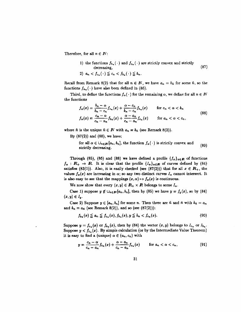
Therefore, for all n E IN:

1) the functions fb .. ( . ) and fe .. ( . ) are strictly convex and strictly decreasing, (87)

2) an < fe .. (- ) ~ en < fb .. ( . ) ~ bn.

Recall from Remark 8(2) that for all n E IN, we have an = bn for some ii, so the functions fa .. ( . ) have also been defined in (86).

Third, to define the functions fa( . ) for the remaining a, we define for all n E IN the functions

for en < a < bn

for an < a < en,

where ii is the unique ii E IN with an = bn (see Remark 8(2)).

By (87(2)) and (88), we have:

for all a E UnEJV[an,bn], the function fa(·) is strictly convex and strictly decreasing.

(88)

(89)

Through (85), (86) and (88) we have defined a profile {Ja}aEEl of functions fa : JR+ ~ JR. It is clear that the profile {/a}aEEl of curves defined by (84) satisfies (83(1)). Also, it is easily checked (see (87(2))) that for all x E JR+, the values fa(x) are increasing in a; so any two distinct curves la cannot intersect. It is also easy to see that the mappings (x, a) ~ fa(x) is continuous.

We now show that every (x, V) E JR+ x JR belongs to some la.

Case 1) suppose V ¢ UnEJV[an , bn ], then by (85) we have V = f ll (x), so by (84) (x, V) E 111·

Case 2) Suppose V E [an, bn ] for some n. Then there are ii and n with bn = an

and bn = an (see Remark 8(2)), and so (see (87(2))):

(90)

Suppose V = fe .. (x) or fb .. (X), then by (84) the vector (x, V) belongs to Ie .. or Ib ... Suppose V < fe .. (x). By simple calculation (or by the Intermediate Value Theorem) it is easy to find a (unique) a E (an, en) with

for an < a < en, (91)

31

so by (88(2)) we have y = !a(x), and hence (x, y) E la. Similarly, if !e .. (x) < y < !b .. (X), then (x,y) E la for some (unique) a E (cn,bn); if !b .. (X) < y, then (x, y) E la for some (unique) a E (bn , cn).

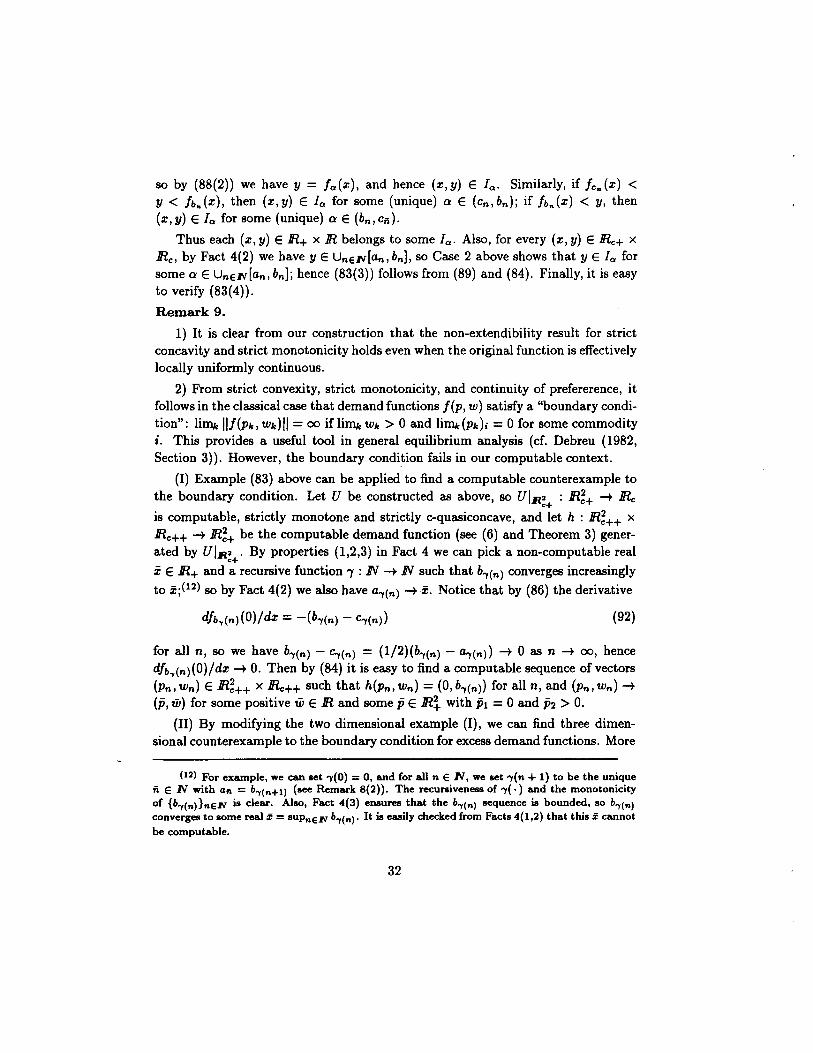
Thus each (x, y) E lR+ x lR belongs to some la. Also, for every (x, y) E lRe+ x lRe, by Fact 4(2) we have y E UnEl'V[an , bn], so Case 2 above shows that y E la for some a E UnEl'V[an , bn ]; hence (83(3)) follows from (89) and (84). Finally, it is easy to verify (83(4)).

Remark 9.

1) It is clear from our construction that the non-extendibility result for strict concavity and strict monotonicity holds even when the original function is effectively locally uniformly continuous.

2) From strict convexity, strict monotonicity, and continuity of prefererence, it follows in the classical case that demand functions !(p, w) satisfy a "boundary condi­tion": lilllk 1I!(plc, wlc)1I = 00 if lilllk Wic > 0 and lilllk(PIc)i = 0 for some commodity i. This provides a useful tool in general equilibrium analysis (cf. Debreu (1982, Section 3)). However, the boundary condition fails in our computable context.

(I) Example (83) above can be applied to find a computable counterexample to the boundary condition. Let U be constructed as above, so UI.fi2 : lR~+ -+ lRe

c+ is computable, strictly monotone and strictly c-quasiconcave, and let h : lR~++ x lRe++ -+ lR~+ be the computable demand function (see (6) and Theorem 3) gener­ated by UI.fi2 . By properties (1,2,3) in Fact 4 we can pick a non-computable real

c+ i E lR+ and a recursive function '1 : IN -+ IN such that b..,(n) converges increasingly to i;(12) so by Fact 4(2) we also have a..,(n) -+ i. Notice that by (86) the derivative

dhy(n) (O)/dx = -(b..,(n) - c..,(n)) (92)

for all n, so we have b..,(n) - Cy(n) = (1/2)(b..,(n) - a..,(n)) -+ 0 as n -+ 00, hence dhy(n)(O)/dx -+ O. Then by (84) it is easy to find a computable sequence of vectors (Pn,wn) E lR~++ x 1Rc++ such that h(Pn,wn) = (O,b..,(n)) for all n, and (Pn,wn)-+ (p, w) for some positive w E lR and some p E lR~ with Pi = 0 and P2 > O.

(II) By modifying the two dimensional example (I), we can find three dimen­sional counterexample to the boundary condition for excess demand functions. More

(12) For example, we can Bet "Y(o) = 0, and for all n E N, we Bet "Y(n + 1) to be the unique n E N with aft = b-y(n+l) (see Remark 8(2». The recursiveness of "Y( .) and the monotonicity of {b-y(n)}nE.N is clear. Also, Fact 4(3) ensures that the b-y(n) sequence is bounded, so b-y(n)

converges to Bome real f& = sUPnE.N b-y(n). It is easily checked from Facts 4(1,2) that this f& cannot

be computable.

32

precisely, it is easy to find a computable consumer (u,w) whose utility function u : lR~+ -+ lRe is strictly c-quasiconcave, strictly monotone, and computable, and endowment w is strictly positive vector in lR~+, and the excess demand function / : lR~++ -+ lR~ defined by /(p) = argmax{u(z) : z E lR~+ & p. z ~ p. w} - w violates the boundary condition. In particular, there is a computable sequence of Pk E lR~++ such that IIPkll = 1 for all k, and (Pkh converges to 0 as k -+ 00, and (f(Pk)h = (f(Pk))3 = 0 for all k, and (f(Pk)h converges to some non-computable i E lR+ as k -+ 00.

REFERENCES

Baigger, G. (1985): "Die Nichtonstrukititat des Brouwerschen Fixpunkstatzes," Arch. Math. Logik, 25, 183-188

Beeson, M. J. (1985). Foundations o/Constructive Mathematics. Heidelberg: Springer­Velag.

Bishop, E. (1967). Foundations of Constructive Analysis. New York: McGraw-Hill.

Bridges, D. S. (1992): "The construction of a continuous demand function for uni­formly rotund preferences," Journal of Mathematical Economics, 21, 217-227.

Chang, C. C and. H. J. Keisler. (1990) Model Theory. Third edition. Amsterdam: North-Holland.

Church, A. (1935): "An Unsolvable Prqblem of Elementary Number Theory," Bul­letin of American Mathematical Society, 41,343-365. (Reprinted in Martin, D., Computability and Unsolvability. New York: Dover, 1958.)

Davis, M. (1983). Computability, Complerity and Languages: Fundamentals of Theoretical Computer Science. New York: Academic Press Inc.

Debreu, G. (1954): "Representation of a Preference Ordering by a Numerical func­tion," in Mathematical Economics, pp. 103-110, by G. Debreu, 1983. Cam­bridge: Cambridge University Press.

- (1982): "Existence of Competitive Equilibrium," in Handbook 0/ Mathematical Economics, Vol. II., ed. by K. Arrow and M. Intriligator. New York: North­Holland.

Grzegorczyk, A. (1955): "Computable Functionals," Fund. Math. 42, 168-202.

Hurwicz, L., and M. K. Richter (1971): "Revealed Preference Without Demand Continuity Assumptions," in Preferences, Utility, and Demand, (John S. Chip­man, Leonid Hurwicz, Marcel K. Richter, and Hugo F. Sonneschein, Eds.), 1971. New York: Harcourt Brace Jovanovich.

33

Kleene, S. C. (1952). Introduction to Metamathematics. New York: D. van Nos­trand.

Ko, K. (1991). Complexity Theory of Real Functions. Boston: Birkhauser.

Kreisel, G. (1958): "Review of H. Meschkowski, Zurrekursiven Functktionentheo­rie," Mathematical Reviews 1958, 238.

Matzkin, R. L., and M. K. Richter (1991): "Testing Strictly Concave Rationality," Journal of Economic Theory, 53, 287-303.

McFadden, D. and M. K. Richter (1990): "Stochastic Rationality and Revealed Stochastic Preference," Chapter 6 in Preferences, Uncertainty, and Opti­mality: Essays in Honor of Leonid Hurwiz, edited by D. McFadden, J. S. Chipman, and M. K. Richter. Boulder: Westview Press.

Moschovakis, Y. N. (1964a): "Notation Systems and Recursive Order Fields," Com­positio Mathematica, 17, 40-70.

- (1964b): "Recursive Metric Spaces," Fundamenta Mathematicae, 15,215-238.

Orevkov, V. P. (1964): "On Constructive Mapping of a Disk into Itself," Trudy Math. Inst. Steklov, 72, 131-161 (Russian). (English transl.: Amer. Math. Soc. Transl. (1971) 100,69-100.)

Pour-EI, M. B., and I. Richards (1989). Computability in Analysis and Physics. New York: Springer-Velag.

Rice, H. G. (1954): "Recursive Real Numbers," Proc. Amer. Math. Soc., 2, 748-791.

Richter, M. K. (1966): "Revealed Preference Theory," Econometrica, 34,636-645.

Richter, M. K., and K. C. Wong (1996a): "Bounded Rationalities and Computable Economies," Working Paper, Department of Economics, University of Min­nesota.

(1996b): "Bounded Rationalities and Definable Economies," Working paper, Department of Economics, University of Minnesota.

Robinson, A. (1963) Introduction to Model Theory and to the Metamathematics of Algebra. Amsterdam: North-Holland.

Simon, H. A. (1959): "Theories of Decision-Making in Economics and Behavioral Science," American Economic Review, 49, 253-283.

-(1978): "Rationality as a Process and as a Product of Thought," American Eco­nomic Review: Papers and Proceedings, 68, 1-16.

Tarski, A. (1951). A Decision Method for Elementary Algebra and Geometry, 2nd, edition. Berkeley and Los Angeles: University of California Press.

34

Turing, A. M. (1936): "On Computable Numbers, with an Application to the Entscheidungsproblem," Proc. London Math. Soc. Ser. 2, 42, 230-265.

- (1950): "Computing Machinery and Intelligence," Mind, 59, 433-460.

Wong, K. C. (1994). Economic Equilibrium Theory: A Computability Viewpoint. Ph.D. dissertation, University of Minnesota.

- (1996): "Computability of Minimizers and Separating Hyperplanes," Mathemat­ical Logic Quarterly, 42, 564-568.

Zaslavskii, I. D. (1962): "Some Properties of Constructive Real Numbers and Constructive Functions" Trudy. Math. Inst. Steklov, 67, 385-457 (Rus­sian). (English transl.: Amer. Math. Soc. Transl., 1966, 57, 1-84.)

35