Compulsory Voting, Turnout, and GovernmentSpending: Evidence from Austria∗

Mitchell HoffmanUniversity of Toronto

Gianmarco LeonUPF and Barcelona GSE

Marıa LombardiUPF

May 31, 2015

Abstract

We study a unique quasi-experiment in Austria, where compulsory voting laws arepassed or rescinded across Austria’s nine states at different times. Analyzing all stateand national elections since World War II, we show that compulsory voting laws withmild sanctions decreased abstention by roughly 50%. However, we find no evidencethat this change in turnout affected spending patterns (in levels or composition) or thepolitical equilibrium. Individual-level data on turnout and political preferences suggestthese results occur because individuals swayed to vote due to compulsory voting aremore likely to be non-partisan and have low interest in politics.

JEL Classifications : H10, D72, P16Keywords: Compulsory voting, Fiscal policy, Incentives to vote

∗Contact: Hoffman mitchell.hoffman@rotman.utoronto.ca, Leon: gianmarco.leon@upf.edu, Lombardi:maria.lombardi@upf.edu. We thank Jeremy Ferwerda, Rui de Figueiredo, Fred Finan, Ted Miguel, JohnMorgan, Gerard Roland, Francesco Trebbi, Dijana Zejcirovic, and seminar participants for helpful comments.Melina Mattos and Nicholas Roth provided outstanding research assistance. Hoffman acknowledges supportfrom the Kauffman Foundation, the National Science Foundation IGERT Fellowship, and the Social Sci-ence and Humanities Research Council of Canada. Leon acknowledges support from the Spanish Ministryof Economy and Competitiveness, through the Severo Ochoa Programme for Centres of Excellence in R&D(SEV-2011-0075) and grant ECO2011-25272.

1 Introduction

Despite the centrality of elections to democracy, in elections around the world, many people

fail to vote. Many European countries have seen a steep decline in turnout rates in the past 30

years, with record low rates in the past two (2009 and 2014) elections for the European Parlia-

ment.1 Ethnic minorities, immigrants, and poor voters in Europe are significantly less likely

to vote, potentially distorting the political process (e.g., Gallego, 2007). In the US, turnout

in national elections is often only around 50%, with large disparities along socioeconomic and

racial lines.2 Such disparities in turnout are believed to cause disadvantaged groups to be

under-served by government (e.g., Meltzer and Richard, 1981; Lijphart, 1997).

One policy solution to help address these issues is to make voting mandatory. As of

2008, thirty-two countries had a compulsory voting (hereafter, “CV”) law in place (Chong

and Olivera, 2008), and a higher number had CV at some point during the last 50 years. In

March 2015, US President Barack Obama proposed the possibility of CV, arguing “It would

be transformative if everybody voted—that would counteract money more than anything. If

everybody voted, then it would completely change the political map in this country. Because

the people who tend not to vote are young, they’re lower income, they’re skewed more heavily

towards immigrant groups and minority groups...There’s a reason why some folks try to keep

them away from the polls.”3 However, little is known empirically about how CV affects voter

behavior, politician behavior, or government policy. CV laws are typically enacted at the

national level, making it difficult to separate causal impacts of the laws from time trends.

We provide robust empirical evidence on the impact of CV laws on turnout, the political

equilibria, and fiscal policy using a unique natural experiment in Austria. Since World War

II, Austria’s nine states have changed their CV laws at different times for different types of

1From http://www.europarl.europa.eu/elections2014-results/en/turnout.html, accessed April 28,2015.

2For example, those with a graduate degree often vote at twice the rate of high schooldropouts (Linz et al., 2007). For evidence on racial disparities in turnout, see, e.g., Timpone(1998). Turnout is lower in midterm than presidential elections, e.g., http://time.com/3576090/

midterm-elections-turnout-world-war-two/.3See, e.g., http://www.cnn.com/2015/03/19/politics/obama-mandatory-voting/, accessed April 28,

2015.

1

elections. Austria provides a compelling case study for several reasons. First, the variation

in CV laws is significant across states and over time (including the abrupt ending of CV for

parliamentary elections due to a 1992 ruling of the Austrian constitutional court), providing

rich variation for quasi-experimental analysis. Second, the penalties for not voting were light,

specifically, fines that were weakly enforced, which is useful for thinking about external va-

lidity (e.g., it seems unlikely that harsh penalties for not voting could be enforced in other

developed countries).4 Third, like the US and many other countries, Austria’s elections ex-

hibit socioeconomic disparities in turnout, with poor and underserved groups being much less

likely to vote than the rich.5

Using state-level voting records on state and national elections from 1949-2010, we find

that CV reduced abstention by roughly 50%, increasing turnout from roughly 80% to 90%.

Impacts on turnout vary somewhat across the three types of elections (parliamentary, state,

and presidential), but are sizable for all three types. Interestingly, however, changes in CV

laws appear to have no impact on election outcomes or state-level spending. These zero

effects are reasonably precisely estimated and are robust to different specifications that deal

with concerns of endogenous changes in CV laws.

How could it be that CV had large impacts on turnout, but did not affect policy out-

comes? Our analysis shows that despite the large increase in turnout, CV did not seem to

affect the political equilibrium: vote shares for liberal parties did not change significantly, nor

did the number of parties running for office, or the victory margin in state or parliamentary

elections. To dig further, we complement our state-level analysis with repeated cross-sections

of individual-level data. We analyze interaction effects of CV laws with voter characteristics

4For the US, consider the large public reaction and legal challenges to making it compulsory to have healthinsurance under the 2010 Affordable Care Act.

5Austria’s disparities in turnout are easily seen in the Austrian Social Survey data discussed below.Of course, there are many important differences between Austria and the US (as well as between Aus-tria and other countries). For Austria and the US, a particularly important difference is that votingrates are considerably higher in Austria (both with and without CV). Thus, there are obviously limita-tions in what our results here may imply for the US. However, high voting rates are observed in manyother countries, both in Europe and elsewhere. In Europe, countries with high voting rates (on the or-der of 80% or higher) include Belgium, Denmark, Germany, Iceland, Italy, Luxembourg, Netherlands andSweden (see http://www.idea.int/publications/voter_turnout_weurope/upload/Full_Reprot.pdf, ac-cessed May 20, 2015).

2

so as to examine which people were swayed to vote because of the CV laws. These voters

were often female, less educated, and low-income. In addition, such voters are more likely to

have low interest in politics, to have no party affiliation, and to be uninformed (as proxied by

newspaper reading). We speculate that such voters may have been more likely to vote for the

leading candidate or to vote “at random,” thereby having little effect on electoral outcomes.

Our paper relates to three main literatures. First, an important literature in political

economy analyzes how changes in turnout and electorate composition affect public policy

(Persson and Tabellini, 2000). The enfranchisement of particular population groups causes

changes in policies, which are more likely to be catered toward these group’s preferences. For

example, Miller (2008) shows that expanding the suffrage rights to women in the US generated

an increase in health expenditures, an issue highly regarded by women at the time. Similarly,

Naidu (2012) provides evidence that laws restricting voting for African-Americans in the late

19th century had sizable impacts on public policy. Analyzing a more recent episode, Fujiwara

(Forthcoming) shows that the adoption of electronic voting in Brazil had sizable impacts

on voting patterns, mainly due to the effective enfranchisement of the poor and illiterate,

leading to increases in health expenses and child health.6,7 Our findings do not contradict

this literature, but complement it, demonstrating that the extent to which changes in turnout

affect policy depends critically on whether these policies affect a group of the population with

specific policy preferences.

Second, it relates to the literature on the determinants of voter turnout. Political scien-

tists and economists have taken substantial interest recently in studying potential interventions

6Other papers in this literature show mixed results of the extension of the voting franchise on redistributivepolicies (e.g., Husted and Kenny, 1997; Rodriguez, 1999; Alesina and Glaeser, 1988; Gradstein and Milanovic,2004; Timpone, 2005; Cascio and Washington, 2014). A common message from this literature is that pub-lic efforts to extend the voting franchise can often significantly affect public policy, making it much morealigned with voters’ preferences. Most of this literature analyzes episodes in which groups with specific policypreferences are de jure or de facto enfranchised, leading elected officials to cater policies toward them.

7There is a recent strand of this literature looking into the electoral and policy effects associated withchanges in voting costs (and thus turnout). Hodler et al. (2015) study the effect of the discontinuous introduc-tion of postal voting across states in Switzerland, and find that this decrease in voting costs led to a sizableincrease in turnout, a lower education of participants, lower knowledge of political issues, and lower govern-ment welfare expenditures. Godefroy and Henry (2014) use rainfall and influenza incidence as instruments forturnout in French municipal elections, and find that an increase in turnout by one percentage point causes adecrease in the municipal budget by more than two percentage points.

3

targeted at increasing turnout, oftentimes using randomized experiments.8 A major lesson

from the experimental literature in advanced democracies is that turnout is sticky (Fujiwara

et al., 2014; Nickerson, 2008). For example, reminding people about the election in various

ways usually has statistically significant, but modest, impacts on turnout. Even fairly signif-

icant interventions, like shaming people who don’t vote by mailing this information to their

neighbors, typically increases turnout only several percentage points (Gerber et al., 2008).9

Turning to non-experimental studies, a significant literature examines the impact of voting

costs, often reaching different results from different changes in costs. For example, Farber

(2009) shows that election holidays and “time-off” have little impact on turnout in the US,

whereas Brady and McNulty (2011) shows that an increase in voting costs due to unexpected

changes in the location of polling costs significantly reduces non-absentee turnout. In terms

of partisan effects, the results are mixed. While turnout in itself is an important outcome to

analyze, one of the reasons why we care about it is because of its ability to ultimately affect

policy. We complement this literature by simultaneously analyzing turnout and government

policy.

Finally, it relates to a small but burgeoning literature analyzing CV. Among a number

of theoretical contributions on this question, Borgers (2004) and Krasa and Polborn (2009)

build on the pivotal voting model to show that compulsory voting (or costly voting) allows

an aggregation of preferences that can increase welfare. On the other hand, Krishna and

Morgan (2011) argue that CV is welfare reducing, since preference intensities can no longer

affect voting participation and, thereby, voting outcomes. Turning to empirical work, in a

cross-country study, Chong and Olivera (2008) show that countries with mandatory voting

have lower income inequality, suggesting that these policies actually democratize societies,

8There is a large family of papers using non-experimental data that analyze different factors that determineparticipation in elections. Weather shocks have been used as exogenous shifts in the cost of voting (e.g., Knack,1994; Gomez et al., 2007; Hansford and Gomez, 2010; Fraga and Hersh, 2010; Gomez et al., 2007), as havegeneral rules of governance (Hinnerich and Pettersson-Lidbom, 2014; Herrera et al., 2014), candidates’ ethnicity(Washington, 2006), and availability of certain information technology (Stromberg, 2004; Enikolopov et al.,2010; Gentzkow, 2006; Gentzkow et al., 2011; Gavazza et al., 2014).

9Green and Coppock (2013) illustrates methodological points on field experiments using examples from thelarge and recent experimental literature on voting.

4

making governments more accountable and forcing them to deliver to the poor. Fowler (2013)

takes advantage of the discontinuous introduction of CV across Australian states in the early

twentieth century and finds that mandatory voting lead to an increase in voter turnout of 24

percentage points in state assembly elections. De Leon and Rizzi (2014) study the Brazilian

case, where voting is voluntary for citizens between 16 and 18 years old, but mandatory

afterward. Using a sample of students in Sao Paolo, they find that CV increases turnout, but

does not affect levels of political information. The results suggest that both recent and long-

term exposure to CV increases knowledge about the party system and party issue platforms,

but might actually contribute to a decrease in familiarity with individual candidates and

representatives. Using a field experiment in Peru providing information about changes in

compulsory voting law fines, Leon (n.d.) shows that a reduction in the cost of abstention

significantly decreases turnout, and consistent with our findings, that the reduction is driven

by uninformed voters, uninterested and centrist voters.

A few political science papers involve the specific case of CV in Austria. The first paper to

explore CV in Austria was Hirczy (1994), who compared overall voting rates between Austrian

states over time using simple graphs on mean turnout rates (no control variables); the graphs

suggest that adoption of CV led to significant increases in turnout. The paper closest to ours

(and contemporaneous with ours) is Ferwerda (2014). Ferwerda (2014) analyzes the effects of

the repeal of CV by the Austrian parliament in 1992 on turnout in parliamentary elections and

on changes in party vote shares. The effects found are relatively small, though consistent with

a theory of party consolidation. Further, even though he uses a much shorter analysis period,

the magnitude of the effects found on electoral participation and party vote shares are broadly

consistent with ours.10,11 Our paper goes beyond these studies in three main ways. First and

foremost, not only do we analyze the political consequences of mandatory voting, but we

also analyze impacts on spending, thereby providing the first micro study (for Austria or any

10Ferwerda (2014) also uses municipal-level data instead of state-level data.11Another contemporaneous paper, Shineman (2014), also uses Austria as a case study to demonstrate the

effects of CV on individual-level political sophistication, finding that both recent and long-term exposure toCV increase voters’ information.

5

other country) to examine how CV affects government spending. Second, we complement the

analysis of aggregate data with individual level information on political preferences and voting

behavior, allowing us to study the shift in the composition of the pool of voters resulting from

CV. Finally, we analyze all elections in Austria since World War II (1949-2010) instead of

just a subset; this enables us to implement a fixed effects analysis allowing for different state

linear trends, which allows us to rule out the concern that the effects observed are only valid

in the short term and that we should expect a reversion to the mean.

The remainder of the paper proceeds as follows. Section 2 provides background on

democratic institutions and CV in Austria. Section 3 describes the data and our estimation

strategy and Section 4 shows the estimation results. Section 5 discusses the mechanisms

behind our results and Section 6 concludes.

2 Democratic Institutions and Compulsory Voting in

Austria

2.1 Democratic Institutions and Budgeting Processes in Austria

Austria is a federal and parliamentary democracy, composed of nine autonomous states. The

National Parliament is composed of two chambers, the National Council (Nationalrat) and the

Federal Council (Bundesrat), with legislative authority vested mostly in the former. National

Council members are directly elected for five-year periods by proportional representation,

whereas members of the Federal Council are elected by the state legislatures.12 Austria’s

executive branch is composed of the Federal President (Bundesprasident), the Federal Chan-

12Historically, no political party has had a majority in parliament, hence coalitions have to be formed. Thetwo dominant political parties (Austrian People’s Party and the Social Democratic Party,OVP and SPO) areusually involved in these coalitions. Once a new government is formed, it generally issues a coalition agreementdocument stating its main policy objectives. The agreements achieved rely on input from the Ministry ofFinance to set yearly deficit targets, and are the primary basis for discussion during the annual budgetnegotiation rounds. However, these documents can’t be considered a medium-term expenditure framework,since they can easily be changed by the partners, and in practice they cease to exist in the waning momentsof the government’s term of office (Blondal and Bergvall, 2007).

6

cellor (Bundeskanzler) and the Federal Cabinet. The Federal President is elected by simple

majority in a popular election for a six-year term, and the candidates are nominated by party

coalitions. The president holds the mostly ceremonial position of head of state. The Federal

Cabinet is composed of the Federal Chancellor, the head of government, and a group of min-

isters, all of whom are appointed by the president. Austrian states are ruled by their own

regional parliament (Landtag), a state government (Landesregierung), and a governor (Lan-

deshauptmann). State parliament representatives are directly elected and serve for five-year

terms.13 Unlike the federal government, state governors are elected by the state parliament.

Ninety-five percent of taxes are collected at the federal level, and are distributed across

the three levels of government (i.e., federal, state, and local) according to Fiscal Equalization

Laws, which last for short periods of time (three to four years) and are established by a con-

sensus between the federal and regional governments (Blondal and Bergvall, 2007). Within

the two lower levels of government, tax revenues are distributed across the different units

according to a formula, which takes into account demographic and revenue criteria, but allo-

cates each state/municipality a fixed percentage of the overall budget. Although the largest

portion of tax revenues are allocated to the central government, state governments receive a

significant part of the total budget, and are responsible for providing a wide array of public

goods and services. In 2006, for example, spending by state governments accounted for 17%

of total spending, with 70% and 13% of spending carried out by the central and municipal

governments, respectively. Furthermore, state governments are responsible for administer-

ing primary education, regional infrastructure, transportation, social welfare and pensions

for state civil servants. There are several areas such as health care, education, and social

welfare, in which the responsibilities of the central and state governments overlap and are

thus co-financed or managed jointly.14 State governments have considerable fiscal autonomy,

reflected in the substantial variation in how they choose to allocate their resources. In the

1980-2012 period, for example, the government of Burgenland devoted 66% of its budget to

13An exception to this is the state of Upper Austria, whose representatives serve for six years.14For further details see the International Monetary Fund Country Report No. 08/189, Austria,:Selected

Issues, https://www.imf.org/external/pubs/ft/scr/2008/cr08189.pdf.

7

welfare expenditures and only 13% to infrastructure spending, whereas the neighboring state

of Lower Austria spent 43% of its resources on welfare, and 40% on infrastructure.

In the postwar period, Austria had four major parties. At the right of the political

spectrum are the People’s Party (OVP), a center-right conservative party originated from the

former Christian Social Party, and the right-wing populist Freedom Party of Austria (FPO). At

the left of the spectrum, we find the Social Democratic Party (SPO) and the Communist Party

of Austria (KPO). Other minor parties such as the Green Party, the Allegiance for the Future

of Austria, and the Liberal Forum have become a recent part of the political scene. There are

five different types of elections contemplated by the Austrian political system: elections for

the National Council (henceforth “parliamentary elections”), for the state parliaments (“state

elections”), for the Federal President (“presidential elections”), and elections for municipal

councils and the European Parliament. Throughout this paper we will focus exclusively on

the first three.

2.2 Compulsory Voting in Austria

Figure 1 summarizes the process by which CV was introduced and later repealed in Austria.

The mandate to vote was established and subsequently eliminated many times throughout

the 1949-2010 period; whether voting was compulsory varied substantially both across and

within states, and depending on the type of election, as can be seen in Figure 2. CV was first

introduced in Austria in the 1929 Constitution. In particular, voting became mandatory for

all citizens in presidential elections, but it was up to each state to determine whether voting

was mandatory or voluntary in parliamentary and state elections (See Appendix B for further

details).

The first presidential election with CV was held in 1951. Up until 1980, there were a total

of seven presidential elections. Voting was mandatory in all of them. However, an amendment

to the Austrian Constitution in 1982 made voting in presidential elections compulsory only in

the states that decided so. Thus, for the 1986 presidential elections, it became up to each state

8

to decide whether to keep mandatory voting or not. The states of Vorarlberg, Tyrol, Styria,

and Carinthia decided to keep CV. Furthermore, Carinthia enacted a law establishing CV

for parliamentary and state elections. The remaining five states abolished CV in presidential

elections after the 1982 amendment.

In 1992, a Federal Constitution amendment by the national parliament withdrew the

power of establishing mandatory voting in the national parliament elections from the states.15

Starting in the 1994 parliamentary elections, voting was optional in all states. After this

constitutional amendment, the states which still had CV in presidential and state parliament

elections started repealing their state laws one by one. In 1993, Carinthia and Styria eliminated

CV for both types of elections. Tyrol repealed CV for state parliament elections in 2002, and

Vorarlberg got rid of it before the 2004 presidential elections. After these elections, Tyrol

finally repealed CV for presidential elections. Thus, the 2010 presidential elections, the last

in our sample, were the first in which voting was voluntary throughout the country.

During the period in which voting was compulsory, local authorities were responsible

for issuing fines against the non-voters failing to provide a reasonable excuse for abstaining.

Sanctions for abstention in presidential elections were initially capped at 1,000 schillings.16

In 2004, the last presidential election in which any state had CV, this sanction could amount

to 72 euros (approximately 72 US dollars in 2015).17 Fines for non-voting in parliamentary

elections were substantially higher. In 1957, for example, while the fines for abstention in

presidential elections were capped at 1,000 schillings, sanctions for non-voting in parliamen-

tary elections could reach up to 3,000 schillings. The national law regulating parliamentary

elections also established that failure to settle this fine was punishable with up to four weeks

in jail.18 However, informal evidence suggests that fines were weakly enforced,19 and formally,

there were a wide range of admissible excuses for not voting, such as illnesses, professional

15Federal Law Gazette No. 470/1992.16Federal Presidential Election Law (Bundesprasidentenwahlgesetz), Article 25.17Federal Presidential Election Law (Bundesprasidentenwahlgesetz) of 2007, Article 23(3).18Federal Parliament Election Law (Nationalrats-Wahlordnung), Article 105 (3).19For example, the website http://www.idea.int/vt/compulsory_voting.cfm describes the sanctions for

not voting as being “weakly enforced” (accessed May 31, 2015).

9

commitments, urgent family matters, being outside the state during the election, or other

compelling circumstances due to which the voter could not go to the polls.20

3 Data and Estimation Strategy

3.1 Data Sources

In the empirical analysis, we draw upon three main sources of information. To analyze the

effect of CV laws on voter turnout, political competition, and public spending, our initial

sample consists of all parliamentary, presidential, and state elections held since the end of

World War II until 2010.21 For each of these elections we hand-collected information on voter

turnout, proportion of invalid ballots, election results, and political competition from the

Austrian Federal Ministry of the Interior’s yearbooks. Secondly, we draw upon detailed annual

information on expenditures by each of the state governments, which is publicly available from

the Austrian Statistical Agency’s website. Unfortunately, this information is only available

since 1980.22 In all of our specifications, we also include state-specific, time-varying covariates

(i.e., total population and unemployment rates) obtained from the Austrian Statistical Agency.

Table 1 shows the descriptive statistics of our data. On average, turnout in all Austrian

elections is relatively high, ranging between 86% in state elections and 90% in parliamentary

elections.23 The average incidence of invalid ballots in these elections is between 2%-4%. Both

in state and parliamentary elections, voting for the main right wing parties is more prevalent

(52%-53%), while voting for the two leading leftist parties is around 40%.24 Furthermore, a

20Federal Presidential Election Law (Bundesprasidentenwahlgesetz), Article 23 and Federal Parliament Elec-tion Law (Nationalrats-Wahlordnung), Article 105 (4).

21In our empirical analysis, we exclude the 1945 elections, just after WWII ended. In the period underconsideration there were 19 parliamentary elections, 12 presidential elections, and around 11-15 state electionsin each of the nine Austrian states.

22This restricts our analysis to 10 parliamentary elections, 6 presidential elections and 6-7 state elections ineach state. In the appendix, we show our main results for turnout, invalid votes and political competition forthe restricted period of 1979-2010, and the magnitude of our coefficients is remarkably similar to the analysisfor the full post war period.

23Turnout is the proportion of registered voters who showed up to the polls. Registration is automatic forall citizens with a permanent residence in the country.

24We consider the sum of votes for OVP and FPO as right wing votes, and the sum of votes for the SPO

10

negligible 8% of votes goes on average to other minor parties. The average number of parties

competing in parliamentary elections is higher than those competing for seats in the state

parliament (6.96 vs. 5.98). We classify expenditures into three broad categories: Administra-

tive expenditures, Social Expenditures, and Infrastructure Expenditures.25 In the 1980-2012

period, a great majority of expenses (54%) were devoted to the social sector, while 25% of all

resources were spent in administration, and the remaining 21% were devoted to infrastructure.

Finally, to understand how CV affects the composition of the electorate, we use the Aus-

trian Social Survey, a nationally representative survey conducted in 1986, 1993, and 2003.26,27

The survey asks respondents standard questions on demographics, socioeconomic status, edu-

cation, and importantly, it inquires about voting behavior, and political and social preferences.

Table 2 shows the descriptive statistics from our individual level data.28 Eighty-eight percent

of respondents report having voted in the previous parliamentary elections. Even though the

data is based on self reports of voting, the national and regional averages resemble quite ac-

curately the actual turnout rates in each of the elections.29 Thirty-three percent of voters in

our sample have a preference for left-wing parties, 31% for right-wing parties, and 7% report

having a preference for other smaller political parties. While the broad majority of voters

identify themselves with a specific political party, a sizeable proportion of voters (30%) report

that they do not have a specific preference for a political party. We see a similar pattern when

we look at party membership. A large majority of the population (82%) reports not being a

affiliated with a political party. While a significant share of our sample declares that they are

and KPO as votes for the left.25Administrative expenditures include spending on elected representatives and general administration, Social

Expenditures comprise expenditures on education, health, arts and culture and social welfare and housing,while Infrastructure Expenditures are those for construction, transport, and security. The yearly expendituredata is expressed in current millions of euros.

26The survey round carried out in 1993 did not include questions on turnout, so we exclude it from ourmain analysis.

27For a general description of the waves of the Austrian Social Survey used, see Haller et al. (1987) andHaller et al. (2005).

28Our sample includes all individuals who reported whether they voted or not in the previous parliamentaryelections. Only 3% of respondents failed to provide this information, and attrition is not correlated to whethervoting was compulsory or not in their state.

29Furthermore, the coefficient measuring the effect of CV on turnout obtained from our estimations withindividual data in Table 9 is strikingly similar to the coefficient from our estimations using state-level officialturnout data.

11

interested in politics (24% are very interested and 40% are somewhat interested), we observe

that 36% is not interested in politics at all. Finally, we proxy for political information using a

question that identifies voters who read the newspaper regularly. Thirty-one percent of voters

report that they don’t regularly read the newspaper.

3.2 Estimation Strategy

We estimate the causal effect of CV laws on turnout, invalid ballots, political competition

and public spending in different elections using a difference-in-difference model in which we

compare the outcomes of interest in states with and without CV. Our baseline specification

is as follows:

yst = α0 + β1CVst +Xstβ2 + δs + νt + γst + εst

where yst is an outcome variable in state s and year/election t. CVst is a dummy variable

indicating whether voting was compulsory in year/election t and state s, Xst is a vector

of state-year covariates (population and the unemployment rate). δs and νt are state and

year/election fixed effects. γst is a set of state-specific linear time trends, and finally εst

is the error term. We run these regressions separately for different types of elections (i.e.,

parliamentary, state, and presidential), and allow for arbitrary correlation structures in the

error terms by clustering our standard errors at the state level. Given the small number

of clusters, our standard errors might be inconsistently estimated (Bertrand et al., 2004).

Following Cameron et al. (2008), we also report wild-bootstrap p-values for the variables of

interest.

Using state level data, we analyze the effect of CV on: (i) turnout and valid ballots; (ii)

left/right vote shares, number of parties, vote shares and margin of victory of the winning

party; and (iii) government expenditures in social services, administration, and infrastructure.

For (i) and (ii), the analysis unit is stateXelection, while when analyzing the impact of CV

on expenditures, the analysis unit is stateXyear. We assume that government spending in

12

the years within a particular electoral period depends on whether voting was compulsory in

the previous election. Thus, if elections takes place in years t and t + 4, we consider that

expenditures in the years spanning from t + 1 to t + 4 are a function of whether voting was

compulsory in t.30 This is a plausible assumption, since most of the elections in our sample

occurred in the last trimester of the year, thus policies implemented by the elected government

would only start having an effect on spending decisions in subsequent years.31

The identification assumption in our main specification is that assignment to CV is

uncorrelated with other state-specific, time varying, observable or unobservable characteristics,

once we have controlled for time invariant, state-specific factors, as well as year-specific, state

invariant factors. For example, if conservative states are more likely to support CV, this

should be absorbed by our state fixed effects. On the other hand, if it is the case that in a

specific year there was a national push for abolishing these types of laws (like, for example in

1982), this effect would be captured by the corresponding year fixed effect. One threat to our

identification assumption is that, even though some of the changes in CV laws were issued

by the federal parliament (e.g., the 1992 repeal of CV in parliamentary elections), and thus

are unlikely to respond to state-specific political dynamics, others changes were issued at the

state level, and these decisions might be related to voting trends. As in any difference-in-

difference model, this is the same as assuming that, conditional on the set of observables and

fixed effects, the trends in voting, political competition, and expenditures in states in which

CV was introduced was the same as in states where voluntary voting was in place; if the

new voting regime had not been enacted, e.g., they have parallel trends in the pre-treatment

period.

The parallel trends assumption would be violated if the states most likely to implement

CV were those in which turnout was downward trending. In this case, an estimation relying

30Due to this, the sample for which we carry out the expenditure and receipt regressions spans the electionsheld in the 1979-2010 period, which in turn determines the expenditures in years 1980-2012.

31In the case of (i), in addition to running separate regressions for each type of election, we also run a pooledregressions using all elections. Further, beyond the reduced form analysis presented above, we also analyzethe effect of (exogenous) changes in turnout on (ii) and (iii) using an instrumental variable approach in whichCVst is used as an instrument for voter turnout. These results are shown in the appendix.

13

on simple fixed effect will understate the effect of CV laws. Similarly, state governments might

find it easier to enact CV laws when turnout is trending upward, since enforcement costs will

be lower in these states. In this case, a fixed effects model would overestimate the results. The

inclusion of state-specific time trends controls for any linear trends in our outcome variables,

and thus partially addresses these concerns. In the next section, we show a set of placebo

and falsification tests supporting the idea that the introduction or abolition of CV laws at

the state level does not seem to be driven by differential trends. Additionally, we include a

regression in which we only consider the change in CV laws issued at the federal level in 1992,

and show that the point estimates are very similar to those found with the full sample.

We confirm the results from our state-level data using individual-level information from

the 1986 and 2003 Austrian Social Survey. In this survey, we have information on whether

each individual voted in the previous parliamentary election (1983 and 2002), and exploit

within and between state variation in CV introduced by the federal abolition of CV between

the surveys (in 1992) to identify the effect on individual level turnout. While in the 2002

parliamentary election none of the Austrian states had CV, three of them (Styria, Tyrol, and

Vorarlberg) had it in the 1983 elections. As in our state-level analysis, we use a difference-in-

difference strategy to estimate the causal effect of CV on turnout:

votedist = α + β1CVst +Xistβ2 + δs + νt + εist

where votedist is a dummy for whether individual i in state s and survey year t voted in

the previous parliamentary election, CVst is a dummy for whether voting was compulsory in

that election in the state where the respondent lives, Xist is a vector of individual covariates

(age, sex, educational attainment, parents’ education, working status, household size, and

community size), δs and νt are state and survey-year fixed effects, and εist an error term.

Our main interest is in the coefficient associated with compulsory voting (CVst). In this case,

to be able to interpret β1 as the causal effect of CV laws on individual voting behavior, we

assume that the trends in individual voting behavior in states that abolished CV after the

14

1983 elections would have remained similar to those states that didn’t, had CV not been

adopted. In the following section, we provide evidence supporting this assumption.

The availability of individual-level information allows us to go further in explaining not

only how much CV affected turnout, but also who is more likely to respond to changes in the

CV laws, and thus help us identify the main channels though which changes in turnout could

affect actual policy outcomes.32 The Austrian Social Survey includes questions that allow us to

characterize voters along several key dimensions: (i) political preferences and party affiliation,

(ii) interest in politics, (iii) political information, and (iv) socioeconomic characteristics (e.g.,

gender, educational attainment, and income). To test whether the effect of CV on turnout

was driven by a particular type of voter, we interact the term of interest in the regression

above with each of these dimensions.33 Specifically, we run the following regression:

votedist =J∑

j=1

[φjGj ist + γjCVst ∗Gj ist] +Xistβ + δs + νt + εist

Our main interest is in γj, the coefficient associated with the interaction between com-

pulsory voting (CVst) and voter characteristics (Gj ist).34

4 Compulsory Voting, Turnout, and Public Spending

4.1 Turnout and Invalid Votes

Even with mild enforcement, as is the Austrian case, CV can affect turnout through the

signaling value of enacting a law. Panel A in Table 3 shows the effects of CV on turnout

32Although the Austrian Social Survey asks about the party individuals voted for in the previous elections,we do not analyze this outcome because 17% of the respondents who report to have voted in the electionsdidn’t answer this question. Furthermore, attrition is differential along individuals’ self-reported politicalpreferences.

33In this set of regressions, we exclude the constant, so we are able to identify which specific group of thepopulation is driving most of the effect.

34For political preferences and income, we have four categories (j = 4); when evaluating whether the effectof CV on turnout is driven by voters with different levels of interest in politics or educational attainment, wehave 3 categories (j = 3). Finally, party membership, our measure of political information, and gender arebinary, and hence, j = 1.

15

within and across Austrian states in the 1949-2010 period. The introduction of CV causes

statistically and economically significant increases in turnout in parliamentary, state, and

presidential elections.

In parliamentary elections, CV increases turnout by 6.5 percentage points, while for state

and presidential elections the effect is of 17.2 percentage points and 9.5 percentage points,

respectively. Pooling all the election data available provides more variability in the data, and

allows for a precise estimation of the year and state fixed effects, as well as better identification

of the state-specific linear trends, which in turn allows for a more precise estimation of our

main effects. In column 4 of Panel A in Table 3, we report the independent effect of CV on

each type of election using the pooled dataset. The introduction of CV increases turnout in

parliamentary elections by 6.6 percentage points, while for state and presidential elections,

the effect is of 8.5 percentage points and 9.2 percentage points, respectively. Note that the

results in the pooled estimation show slightly lower point estimates than in the previous

regressions, and this is particularly the case for state elections, for which we have a smaller

sample size. Given abstention rates of 12%-24% when voting is voluntary, this effect implies

a reduction in abstention ranging from 39% to 55%, depending on the type of election. In

all regressions, we report standard errors clustered at the state level in parenthesis, and the

wild-bootstrap p-values for the coefficients of interest are reported in square brackets. The

statistical significance of the results remains unchanged when looking at either.

Mandating voting can increase turnout by drawing voters who have a low intrinsic value

for voting, uninterested voters, or new voters who might not be familiar with the voting

process. If this is the case, we might expect the proportion of invalid ballots to rise when

more people are mandated to vote. As shown in Panel B of Table 3, the increase in turnout

is paired with a statistically significant increase in invalid votes. In elections when voting is

voluntary, the share of invalid votes ranges between 1.5% and 3.8%. Based on the results in

the preferred specification (column 4), we see that the introduction of CV increases the share

of invalid votes by 0.9–1.8 percentage points, depending on the type of election. Even though

16

the increase in turnout associated with CV is also conducive to a higher proportion of invalid

votes, there is certainly not a one-to-one relation. That is to say, for every 10 people who are

driven to vote due to CV, only 1.5–3 of them issue an invalid ballot, while the others correctly

vote for a party or candidate. Hence, an increase in turnout of this magnitude could very well

result in a shift in the election results, and in the policies being implemented.35

4.2 Public Spending

The introduction of CV leads to a significant increase in turnout of about 9 percentage points,

and the large majority of this increase is driven by valid votes. An increase in participation

rates can potentially affect government spending in several ways. Depending on the compe-

tencies of the elected body analyzed, it could increase the overall size of the budget by pushing

the local government or local parliamentarians to negotiate larger budgets from the federal

government, or by increasing taxation. Alternatively, if preferences for public goods in the

participating electorate are now different, the government might also change the distribution

of public spending, keeping the size of the overall budget constant, but shifting it between

sectors. Previous evidence suggests that a large increase in turnout, as the one we observe in

Austria, lead to changes in policy outcomes (e.g., Miller, 2008; Fujiwara, Forthcoming).

In the Austrian context, if anything, we should expect increases in turnout in different

elections to affect different parts of the budgetary process. As discusses in section 2.1, given the

ceremonial role of the federal president, we don’t expect to see any effects of CV in presidential

elections on spending36. On the other hand, the national parliament does decide on the amount

of money that each state and local government gets, so if anything, we should observe changes

in the parliamentarian’s constituents affecting the state’s total budget, but not its sectoral

35Given that the analysis of the effects of CV on fiscal behavior is performed only for those years for whichexpenditure data is available (1979–2010), we rerun the analysis from Table 3 on a comparable sample inAppendix table B.1. The results shown for turnout and invalid votes are comparable to the ones in the fullsample.

36As a placebo test, we run the regressions estimating the effect of CV in presidential elections on fiscalbehavior at the state level, and as expected, we do not find any effects. These results are shown in Appendixtable B.2

17

distribution. Finally, given that state parliaments nominate a share of the members of the

Federal Council, we should expect changes in the state parliamentarian’s political incentives

to affect the national distribution of the budget. Likewise, state parliaments are in charge of

preparing the state’s budget, and thus laws that affect this level of government should have

an effect on the sectoral distribution of state spending. In this section, we turn our attention

to the effects of CV on fiscal policy at the state level. Because data on public spending is only

available for the years 1980-2012, we limit our analysis to that period.

In the subsequent analysis, we focus on total state expenditures, as well as their compo-

sition: administrative, welfare, and infrastructure expenditures. For each spending category,

we independently analyze three different measures of fiscal policy, which are intended to test

the different mechanisms described above: (i) the log levels, (ii) the log per capita, and (iii)

as a percentage of the total budget. Using a similar estimation framework as in the previous

section, the results of our reduced form regressions for parliamentary and state elections are

shown in Table 4. Given the competences of the federal and state parliaments, it is surprising

that changes in laws affecting the incentives of parliamentarians do not manifest themselves in

economic or statistically significant effects on the level or composition of expenditures. Over-

all, we find no evidence of an effect of CV on the amount or composition of public expenditures,

both for parliamentary and state elections. In all regressions, the estimated coefficients are

very close to zero, and the clustered standard errors as well as the wild-bootstrap p-values indi-

cate that there is no statistical relationship between CV and total budget or its composition.37

Given the zero effect found in the reduced form in Table 4, it is not surprising that when we

use an instrumental variable approach, where we estimate the effect of turnout (instrumented

by CV) on expenditures, we also find a zero effect (see Table B.3 in the appendix.)

37We only find one significant coefficient out of the 33 regressions that we show in Table 4 and Appendixtable B.2, for the effect of CV in state elections on the percentage of the budget going to welfare.

18

4.3 Robustness Checks

In order to be able to causally interpret the results presented in Sections 4.1 and 4.2 we need

to assume that, once we control for the set of fixed effects and state trends, assignment to CV

is uncorrelated with the error term. This assumption would be violated if states that chose to

implement CV did so as a response to secular trends in our main variables of interest. This is

equivalent to assuming that, had CV never been introduced, states where it was introduced

would have followed a similar trend as in those where voting was always voluntary, a standard

assumption in any difference-in-difference framework. In this section, we provide a set of

placebo and falsification tests supporting our identifying assumption.

As mentioned in Section 2.2, in our study period there is one change in CV laws that is

unrelated to any state–year specific characteristic, namely, the one introduced by the federal

government in 1992.38 This Federal Constitution amendment withdrew the prerogative of

establishing mandatory voting in the national parliament elections from the states. Effectively,

while some states already had voluntary voting, others were forced to adopt it.

The results in Table 5 show the difference-in-difference regression limiting our sample to

the parliamentary elections in the electoral periods between 1986 and 2011, in which the only

change in CV laws was the one enacted in 1992. This law forced Vorarlberg, Styria, Tyrol

and Carinthia to eliminate CV in parliamentary elections.39 The magnitude and statistical

significance of the results is remarkably similar to those shown in Tables 3 and 4. The re-

peal of CV in 1992 causes a decrease in turnout in parliamentary elections of 9.8 percentage

points, and an increase in invalid ballots of 1.3 percentage points. Likewise, in neither of our

38Ferwerda (2014) uses this federal change in legislation to explore changes in the political equilibrium, andargues that, given that it was issued at the federal level, it is independent to the political dynamics at thelocal level.

39The estimation equation is given by: yst = α0 + α1CVs ∗ Pret +Xstβ + δs + νt + εst. As in our previousspecifications, yst is an election outcome variable or expenditures in state s and year t; CVs is a dummyvariable indicating whether voting was compulsory in state s before the 1992 constitutional amendment,Pret is a dummy for the elections before 1992, Xst is a vector of state–year covariates (population and theunemployment rate), δs and νt are state and year fixed effects and εst is the error term. Our interest liesin the coefficient that measures the difference-in-difference between states with and without CV, before andafter the reform, α1. For comparison with previous tables, we introduce the “Pre” instead of “Post” dummybecause after 1992, CV was repealed, rather than introduced.

19

specifications do we find that CV affects fiscal policy. These results suggest that any other

changes in CV (besides the 1992 one) are unlikely to be correlated with trends in the main

dependent variables.

The parallel trend assumption can also be shown graphically. Figure 3 shows the evo-

lution of turnout, invalid votes, and total, administrative, welfare, and infrastructure expen-

ditures in the same analysis period (1986-2011), for states that never had CV and those that

were mandated to eliminate it in 1992. States that had CV before 1992 had higher turnout

and more invalid ballots, but importantly, after the law is abolished, the trends in these vari-

ables run parallel to the ones in states that did not have CV before 1992. Similarly, in our

four expenditure variables, for which we do not observe an effect of the elimination of CV,

the trends for both types of states run parallel during the whole study period.

To further alleviate the concerns that CV laws might have been introduced responding

to changes in our dependent variables of interest (e.g., they could have been a response to

declining turnout rates), in Table 6 we include leads and lags of our main independent variable

in our preferred specification for turnout and invalid votes. If it were the case that CV laws

responded to changes in turnout, we would expect turnout in period t to be correlated to

either CV in t+ 1 or CV in t− 1. The results show that, besides the contemporaneous effect

of CV on turnout and invalid votes, the introduction of CV in the previous election or next

electoral period has no effect on our variables of interest. The estimated effects for the three

types of elections show a precise zero of all the lags and leads of our independent variable.40

We report the results of the same analysis for our public spending regressions in Table 7. A

potential concern is that authorities anticipate the introduction/repeal of CV laws and alter

the level or composition of public spending before the law change takes place. If this were

the case, we would observe a correlation between public spending in year t and CV in t + 1.

Alternatively, any delays in the reaction of public spending to changes in CV laws would

lead to a correlation between CV in t − 1 and public spending in year t, which would not

40One exception is the surprisingly significance of the coefficient of the lead of CV for presidential elections.However, the estimated coefficient is negative, which goes against our main effects.

20

be captured in our baseline specification. As seen in Table 7, public spending is uncorrelated

whether voting was compulsory in the past, current, or posterior electoral period for all types

of elections.

Taken together, the results shown in Figure 3 and Tables 5, 6, and 7 provide evidence

supporting the parallel trend assumption, and rule out the potential reverse causation between

turnout and CV laws.

5 Understanding the “Null Effect” on Policy Outcomes

How could it be that CV had sizable impacts on turnout, increasing the number of valid votes,

but did not affect policy outcomes? One potential explanation for these results is that, even

though more voters attend to the polls, the political choices of voters who would have otherwise

abstained are, on average, similar to the ones of voters who would have gone to the polls even

in the absence of CV. Alternatively, it could also be the case that the victory margins are, on

average, larger than the increase in turnout, hence even if everyone voted for the same party,

this would not affect the electoral result. In a standard median voter model (Downs, 1957), a

change in the preferences of the median voter leads to changes in candidate’s platforms, and

hence, to changes in policy. Alternatively, citizen-candidate models (Besley and Coate, 1997;

Osborne and Silvinski, 1996) predict that when parties cannot credibly commit to implement

policies that are inconsistent with their ideology, variations in the composition of the electorate

will affect the policies implemented through their impact on the identity/preferred policies

of the party that gets elected. In the context of Austria, the results observed so far, are

consistent with either theoretical frameworks.

If new voters do not make significantly different political choices, compared to those

voters who participate even under voluntary voting, we would not expect the identity of the

median voter to change, and hence shouldn’t observe changes in policies. Unlike other studies

in the literature analyzing large increases in turnout due to de jure or de facto enfranchise-

ment of very specific groups of the electorate (e.g., women in Miller (2008), the poor and

21

illiterate in Fujiwara (Forthcoming), and African-Americans in Naidu (2012)), there are no a

priori reasons to believe that voters who participate in the elections because of the CV laws

make significantly different political choices than those who participate even when voting is

voluntary. In the subsequent analysis, we explore whether CV laws caused changes in the

political equilibrium, and identify marginal voters affected by the introduction of CV.

5.1 Electoral Competitiveness and Partisan Advantage

Table 8 tests whether the introduction of CV had any effects on the identity of the elected

politician, political competition, or her victory margin. We estimate a similar regression as

in the Section 4.1, but use as dependent variables the percentage of votes to the left or right

wing parties, the number of parties, the share of votes of the winning party and its margin of

victory (i.e., the difference in vote share between the winning party and the runner-up).

As shown in Table 8, CV does not lead to substantial changes in the results or the

competitiveness of the elections.41 For both parliamentary and state elections, CV does not

affect the share of votes going to the right or left parties.42 Further, there is no response

from the political supply: the number of parties remains constant at about 6.9 and 6 for

parliamentary and state elections, respectively. Finally, the party that wins the election does

not receive a significantly different proportion of votes under CV, compared to states and

elections in which voting is voluntary.43

In a related paper, Ferwerda (2014) exploits the 1992 constitutional change to analyze

41We do not perform these regressions for presidential elections because parties do not run as separate entitiesin those races. Instead, they form coalitions that cross party lines and change over time, making it impossibleto identify the proportion of votes for right and left wing parties. In 1974, for e.g., the candidate nominatedby the socialist SPO won the presidential election. This candidate was reelected in the 1980 elections, wherehe received support from the SPO but also from the right-wing OVP party.

42Although we only report the results of our regressions considering vote shares for left (SPO + KPO) andright wing (OVP + FPO) parties, we also run regressions using the individual vote shares of these parties andfind no effect. We also check whether there was any impact on voter polarization, and find that there is noeffect of CV on the sum of vote shares for the two main parties (SPO and OVP).

43Appendix Table B.4 shows the results for the sample 1979-2010. The results are comparable to those inTable 8. We find relatively larger point estimates for the effects of CV on party vote shares, but they are notstatistically significant. Only for the case of votes for the left wing parties in Parliamentary elections do wefind a statistically significant impact of CV; however, if we focus on the wild-bootstrapped p-values (the mostrobust), the coefficient is not significant at the conventional levels.

22

the effects of political participation on electoral results. Using municipality level data from

the 1990 and 1994 elections (before and after the change), he finds statistically significant but

fairly small effects on the vote share for minor parties, as well as an increase in votes for the

SPO (left wing party). The magnitude of the results found are consistent with our findings,

particularly with the magnitude of the coefficients found when restricting our analysis period

(Appendix Table B.4). However, the focus of our paper is on explaining the potential effects

of CV on fiscal behavior, and even though there might be an (insignificant) effect on party

vote shares, they are small enough that they do not affect the election outcomes.

Overall, the results in Table 8 show that the introduction of CV did not lead to changes

in party vote shares, electoral competition, or partisan advantage. If the Austrian political

process follows the workings of a citizen-candidate model (Besley and Coate, 1997; Osborne

and Silvinski, 1996), the fact that the increase in turnout was not paired with changes in the

political equilibria is consistent with a null impact of CV on public expenditure in the period

under consideration.

5.2 Composition of the Electorate

In this section, we use individual level data on political preferences and demographics from two

rounds of the Austrian Social Survey (1986 and 2003) to explore whether the null effects of CV

on economic policies and the political equilibria can be explained by the identity of marginal

voters who are driven to the polls only due to the introduction of CV. For identification, we

exploit the fact that between the two survey rounds CV laws changed in some states.

For comparison purposes, the first column of Table 9 resembles the baseline specification

from Table 3 at the individual level. The introduction of CV leads to an increase in turnout

of 5.8 percentage points, slightly lower than the one shown with aggregate, state-level data.

We must bear in mind that in these regressions we rely on self-reported data, which might

measure turnout with error. As long as this measurement error is classical, our results should

23

be attenuated.44

In columns (2)–(4) of Table 9 we show how the demographic composition of the electorate

changes with CV. Rational choice models of voting suggest that an increase in the cost of

abstention resulting from CV should drive low-income voters to the polls (Downs, 1957; Riker

and Ordeshook, 1968). Consistent with previous literature (Matsusaka, 1995; Lijphart, 1997;

Shue and Luttmer, 2009) we find that women, voters with low educational attainment, and

low income, seem to be the ones who respond more often to CV laws, whereas men, highly

educated people, and relatively high income voters are likely to participate even in the absence

of CV laws.45

This demographic composition of the electorate should lead to changes in the preferences

of the median voter, in the political equilibria, and therefore in economic policies, if the

demographic characteristics of new voters correlate with political preferences. In Table 10

we explore the latter dimension. The results show that marginal voters who respond to the

introduction of mandatory voting are non-partisan, and have a low subjective value of voting

(as measured by their interest in politics). Specifically, while we do not observe an effect of CV

on voters who declare preferences for right, left, or centrist parties, those who do not declare

partisan preferences are 14.2 percentage points more likely to vote when facing CV. Along the

same lines, Column (2) shows that voters who are not members of any party respond to these

laws by showing up at the polls 8.4 percentage points more often, while members of political

parties vote regardless of the legislation. Consistent with these results and with previous work

(Lassen, 2005), voters who respond to the legislative incentives to vote are the ones who declare

themselves as not being interested in politics and the uninformed (Column 3 and 4). Overall,

the results in Table 10 show that marginal voters do not have clear partisan preferences, and

in general, do not seem to attach a high intrinsic value to political participation.

Although compulsory voting seems to have shifted the demographic characteristics of the

44Given that our coefficient for CV is slightly lower than the one obtained in our regressions using aggregatestate-level data, one need not be concerned about higher over-reporting by individuals for which voting wascompulsory.

45The results regarding the effect of CV for people with different income levels should be taken with care,as there were a lot of individuals who did not report their household income.

24

median voter in terms of gender, educational attainment and income, this does not correlate

with the median voter’s political choices. All in all, the marginal voter turning out to vote

as a result of the enactment of compulsory voting laws seems to be an apathetic voter who

does not issue, on average, a different vote from the voters who were already participating in

voluntary elections. If the choices of the average voter are not shaped by the implementation

of compulsory voting, it should not be surprising that these laws do not impact the policies

implemented nor the identity of the elected party. Alternatively, these results are also con-

sistent with a citizen candidate framework in which, even though the identity of the median

voter changes, we do not observe changes in policy outcomes.

6 Conclusion

Although compulsory voting (CV) is often viewed as a way to foster voter turnout and con-

sequently improve the representativeness of the political process, relatively little is known

how CV causally affects voter participation and, in particular, how it affects economic policy.

In this paper, we analyze the impacts by leveraging a unique quasi-experiment in Austria.

Exploiting substantial variation in CV laws across Austria’s nine states, we find that CV

increased turnout from roughly 80% to 90%, reducing abstention by roughly 50%. This oc-

curred even though penalties for not voting were mild. However, the increase in turnout

did not seem to affect state-level spending (either in levels or shares of sectoral spending) or

electoral outcomes.

How should our results be interpreted? Using individual-level data, we find that people

induced to vote by CV seem to be those with no preference between political parties. Thus,

even though voters affected by CV are also more likely to have lower education and lower

income, our results are not inconsistent with median voter models. Our results are also con-

sistent with citizen candidate models where candidates implement preferred policies despite

a change in the identity of the median voter. While our results do not crisply distinguish be-

tween different theoretical models of voting, they provide causal evidence (previously lacking)

25

that CV laws need not have significant impacts on government spending, even if they have

large impacts on who is voting. We believe this is important evidence for the policy debate

regarding CV.46

While our results are specific to Austria, we believe our findings are relevant for other

advanced democracies where reforms to increase political participation (such as CV laws) are

being evaluated. Voter turnout levels in Austria (both with and without CV) have generally

been high (at least relative to the US), but high turnout levels are shared by many other

countries, both in Europe and elsewhere. The advantage of analyzing the whole postwar

period, rather than a single historical change in electoral laws, is that it allows us to rule

out that the effects observed are due to specific historical contexts, providing more external

validity to our results. It is less clear how our results would extrapolate to a country like the

US.47 More research on the impacts of compulsory voting is clearly warranted.

46That is, it provides a counterpoint to the argument that CV laws are necessarily transformative forgovernment policy.

47In terms of turnout, US voters are are sometimes viewed as being less trustful of government than votersin Europe, so it is not clear that US voters would react substantially to small fines. On the other hand,Austria had a relatively high turnout rate to begin, so one might imagine that our findings would form a“lower bound” on impacts for reforms implemented in countries with low turnout. In terms of spending, it ispossible that CV laws could have different impacts on presidential instead of parliamentary systems, thoughwe do not have strong priors that this would be the case.

26

References

Alesina, Alberto and Edward L. Glaeser, “Credibility and Policy Convergence in a Two-

Party System with Rational Voters,” American Economic Review, 1988, 78 (4), 796–805.

Bertrand, Marianne, Esther Duflo, and Sendhil Mullainathan, “How Much Should

We Trust Differences-in-Differences Estimates?,” Quarterly Journal of Economics, 2004,

119 (1), 249–275.

Besley, Timothy and Stephen Coate, “An Economic Model of Representative Democ-

racy,” Quarterly Journal of Economics, 1997, 112 (1), 85–114.

Blondal, Jon R. and Daniel Bergvall, “Budgeting in Austria,” OECD Journal on Bud-

geting, 2007, 7, 1–37.

Borgers, Tilman, “Costly Voting,” American Economic Review, 2004, 94 (1), 57–66.

Brady, Henry and John McNulty, “Turning Out the Vote: The Costs of Finding and

Getting to the Polling Place,” American Political Science Review, 2011, 5 (1), 1–20.

Cameron, A. Colin, Jonah B. Gelbach, and Douglas L. Miller, “Bootstrap-Based

Improvements for Inference with Clustered Errors,” The Review of Economics and Statistics,

May 2008, 90 (3), 414–427.

Cascio, Elizabeth U. and Ebonya Washington, “Valuing the Vote: The Redistribution

of Voting Rights and State Funds Following the Voting Rights Act of 1965,” The Quarterly

Journal of Economics, 2014, 129 (1), 376–433.

Chong, Alberto and Mauricio Olivera, “Does Compulsory Voting Help Equalize In-

comes?,” Economics and Politics, 2008, 20 (3), 391–415.

Downs, Anthony, An Economic Theory of Democracy, New York: Harper, 1957.

27

Enikolopov, Ruben, Maria Petrova, and Ekaterina Zhuravskaya, “Media and Political

Persuasion: Evidence from Russia,” American Economic Review, 2010, 111 (7), 3253–3285.

Farber, Henry, “Increasing Voter Turnout: Is Democracy Day the Answer?,” Working

Paper, Princeton University 2009.

Ferwerda, Jeremy, “Electoral Consequences of Declining Participation: A Natural Experi-

ment in Austria,” Electoral Studies, 2014, 35, 242–252.

Fowler, Anthony, “Electoral and Political Consequences of Voter Turnout: Evidence from

Compulsory Voting in Australia,” Quarterly Journal of Political Science, 2013, 8 (2), pp.

159–182.

Fraga, Bernard and Eitan Hersh, “Voting Costs and Voter Turnout in Competitive Elec-

tions,” Quarterly Journal of Political Science, 2010, 5, 339–356.

Fujiwara, Thomas, “Voting Technology, Political Responsiveness, and Infant Health: Evi-

dence from Brazil,” Econometrica, Forthcoming.

, Kyle Meng, and Tom Vogl, “Estimating Habit Formation in Voting,” 2014.

Gallego, Aina, “Unequal Political Participation in Europe,” International Journal of Soci-

ology, 2007, 37 (4), 10–25.

Gavazza, Alessandro, Mattia Nardotto, and Tommaso Valletti, “Internet and Politics:

Evidence from UK Local Elections and Local Government Policies,” 2014.

Gentzkow, Matthew, “Television and Voter Turnout,” Quarterly Journal of Economics,

2006, 121 (3), 931–972.

, Jesse M. Shapiro, and Michael Sinkinson, “The Effect of Newspaper Entry and Exit

on Electoral Politics,” American Economic Review, 2011, 101 (7), 931–972.

28

Gerber, Alan S., Donald P. Green, and Christopher W. Larimer, “Social Pressure

and Voter Turnout: Evidence from a Large-Scale Field Experiment,” American Political

Science Review, 2008, 102 (01), 33–48.

Godefroy, Rafael and Emeric Henry, “Voter Turnout and Fiscal Policy,” 2014. Mimeo.

Gomez, Brad, Thomas Hansford, and George Krause, “The Republicans Should Pray

for Rain: Weather, Turnout, and Voting in U.S. Presidential Elections,” Journal of Politics,

2007, 69, 649–663.

Gradstein, Mark and Branko Milanovic, “Does Libert = Egalit? A Survey of the

Empirical Links between Democracy and Inequality with Some Evidence on the Transition

Economies,” Journal of Economic Surveys, 2004, 18 (4), 515–537.

Green, Donald P. and Alexander Coppock, Field Experiments: Design, Analysis and

Interpretation, Brookings Institution Press, 2013.

Haller, Max, Kurt Holm, and R. Oldenbourg Verlagr, Werthaltungen und Lebens-

formen in sterreich. Ergebnisse des Sozialen Survey 1986, Munich: R. Oldenbourg Verlag,

1987.

, Wolfgang Schulz, and Alfred Grausgruber, sterreich zur Jahrhundertwende.

Gesellschaftliche Werthaltungen und Lebensqualitt 19862004, Wiesbaden: Verlag fr Sozial-

wissenschaften, 2005.

Hansford, Thomas and Brad Gomez, “Estimating the Electoral Effects of Voter

Turnout,” American Political Science Review, 2010, 104 (2), 268–288.

Herrera, Helios, Massimo Morelli, and Thomas Palfrey, “Turnout and power sharing,”

The Economic Journal, 2014, 124 (574), F131–F162.

29

Hinnerich, Bjorn Tyrefors and Per Pettersson-Lidbom, “Democracy, Redistribution,

and Political Participation: Evidence From Sweden 19191938,” Econometrica, 2014, 82 (3),

961–993.

Hirczy, Wolfgang, “The Impact of Mandatory Voting Laws on Turnout: A Quasi-

Experimental Approach,” Electoral Studies, 1994, 13 (1), 64–76.

Hodler, Roland, Simon Luechinger, and Alois Stutzer, “The Effects of Voting Costs

on the Democratic Process and Public Finances,” American Economic Journal: Economic

Policy, 2015, 7 (1), 141–171.

Husted, Thomas A. and Lawrence W. Kenny, “The Effect of the Expansion of the

Voting Franchise on the Size of Government,” Journal of Political Economy, 1997, 105,

54–82.

Knack, Steve, “Does Rain Help Republicans? Theory and Evidence on Turnout and Vote,”

Public Choice, 1994, 79, 187–209.

Krasa, Stefan and Matthias K. Polborn, “Is mandatory voting better than voluntary

voting?,” Games and Economic Behavior, 2009, 66 (1), 275–291.

Krishna, Vijay and John Morgan, “Overcoming Ideological Bias in Elections,” Journal

of Political Economy, 2011, 119 (2), 183–211.

Lassen, David Dreyer, “The Effect of Information on Voter Turnout: Evidence from a

Natural Experiment,” American Journal of Political Science, 2005, 49 (1), 103–118.

Leon, Fernanda Leite Lopez De and Renata Rizzi, “A Test for the Rational Ignorance

Hypothesis: Evidence from a Natural Experiment in Brazil,” American Economic Journal:

Economic Policy, 2014, 6 (4), 380–398.

Leon, Gianmarco, “Turnout, Political Preferences and Information: Experimental Evidence

from Peru.”

30

Lijphart, Arend., “Unequal Participation: Democracys Unresolved Dilemma,” American

Political Science Review, 1997, 91 (1), 1–14.

Linz, Juan, Alfred Stephan, and Yogendra Yadav, Democracy and Diversity, New

Delhi: Oxford University Press, 2007.

Matsusaka, John G., “Fiscal Effects of the Voter Initiative: Evidence from the Last 30

Years,” Journal of Political Economy, 1995, 103 (3), 587–623.

Meltzer, Allan H. and Scott F. Richard, “A Rational Theory of the Size of Government,”

The American Political Science Review, 1981, 89 (5), 914–927.

Miller, Grant, “Womens Sufrage, Political Responsiveness, and Child Survival in American

History,” The Quarterly Journal of Economics, 2008, 123 (3), 1287–1327.

Naidu, Suresh, “Suffrage, Schooling, and Sorting in the Post-Bellum U.S. South.,” 2012.

Nickerson, David W., “Is Voting Contagious? Evidence from Two Field Experiments,”

American Political Science Review, 2008, 102 (01), 49–57.

Osborne, Martin J. and Al Silvinski, “A Model of Political Competition with Citizen-

Candidates,” The Quarterly Journal of Economics, 1996, 111 (01), 65–96.

Persson, Torsten and Guido Tabellini, Political Economics: Explaining Economic Policy,

Cambridge MA: MIT Press, 2000.

Riker, William H. and Peter C. Ordeshook, “A Theory of the Calculus of Voting,” The

American Political Science Review, 1968, 62 (1), 25–42.

Rodriguez, F. C, “Does Distributional Skewness Lead to Redistribution? Evidence from

the United States,” Economics and Politics, 1999, 11, 171–199.

Shineman, Victoria, “Isolating the Effect of Compulsory Voting Laws on Political So-

phistication: Exploiting Intra-National Variation in Mandatory Voting Laws Between the

Austrian Provinces,” 2014.

31

Shue, Kelly and Erzo FP Luttmer, “Who misvotes? The effect of differential cognition

costs on election outcomes,” American Economic Journal: Economic Policy, 2009, 1 (1),

229–257.

Stromberg, David, “Radio’s Impact on Public Spending,” Journal of Economics, 2004, 119

(1), 589–621.

Timpone, Richard J., “Structure, Behavior, and Voter Turnout in the United States,” The

American Political Science Review, 1998, 92 (1), pp. 145–158.

, “Demokratische Beteiligung und Staatsausgaben: Die Auswirkungen des Frauenstimm-

rechts,” Swiss Journal of Economics and Statistics, 2005, 141 (4), 617–650.

Washington, Ebonya, “How Black Candidates Affect Voter Turnout,” Quarterly Journal

of Economics, 2006, 121 (3), 979–998.

32

Fig

ure

1:E

volu

tion

ofC

VL

aws

(191

8-20

10)

19

18

: E

nfr

anch

isem

ent

of

wo

men

sp

ark

s d

ebat

e o

n C

V

19

29

Co

nst

itu

tio

nal

am

end

men

t:

(i)

Pre

roga

tive

of

eac

h s

tate

to

hav

e C

V in

par

liam

enta

ry a

nd

sta

te

elec

tio

ns –

CV

in

Ty

rol

an

d

Vo

rarl

be

rg

(ii)

Pre

sid

ent

elec

ted

by

po

pu

lar

vote

–C

V i

n a

ll s

tate

s

19

31

: Fir

st p

resi

den

tial

el

ecti

on

un

der

CV

su

spen

ded 1

93

4

19

45

: en

d o

f W

WII

:

(i)

19

29

Co

nst

itu

tio

n r

esto

red

(ii)

Par

liam

ent

and

sta

teel

ecti

on

s u

nd

er n

atio

nal

ele

ctio

nla

w –

no

CV

19

49

par

liam

enta

ry a

nd

sta

te

elec

tio

ns:

CV

in

Ty

rol,

Vo

rarl

be

rg a

nd

S

tyri

a

19

51

: fir

st p

resi

den

tial

el

ecti

on

wit

h C

V i

n a

ll s

tate

s

19

82

: CV

in

pre

sid

enti

al e

lect

ion

s b

ecam

e d

ecis

ion

of

each

sta

te –

CV

on

ly i

n T

yro

l,

Vo

rarl

be

rg, S

tyri

a a

nd

Ca

rin

thia

19

86

: Ca

rin

thia

en

act

ed

CV

la

wfo

r p

arli

amen

t an

d s

tate

elec

tio

ns

Co

nst

itu

tio

nal

am

end

men

t a

bo

lish

ed

CV

in

p

arl

iam

en

tary

ele

ctio

ns

20

10

: Fir

st p

resi

den

tial

el

ecti

on

wit

h v

olu

nta

ry

voti

ng

in

all

sta

tes

19

93

-20

07

: C

arin

thia

, St

yria

, Tyr

ol a

nd

V

ora

rlb

erg

eli

min

ate

CV

in

sta

te a

nd

pre

sid

en

tia

l e

lect

ion

s1

98

2-1

98

6 19

92

33

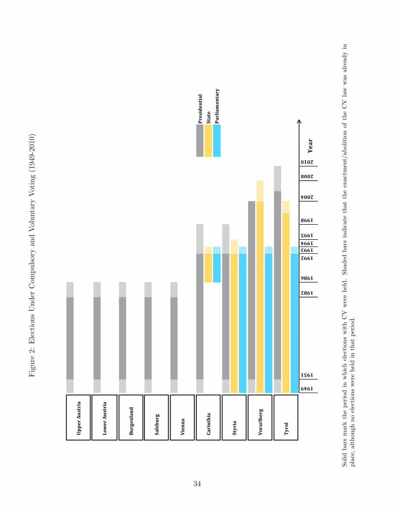
Fig

ure

2:E

lect

ions

Under

Com

puls

ory

and

Vol

unta

ryV

otin

g(1

949-

2010

)

Pre

sid

en

tia

l

Sta

te

Pa

rlia

me

nta

ry

1949

1951

1982

1986

1992

1993

1994

1995

1998

2004

2008

2010

Sty

ria

Vo

rarl

be

rg

Ty

rol

Up

pe

r A

ust

ria

Lo

we

r A

ust

ria

Bu

rge

nla

nd

Sa

lzb

urg

Vie

nn

a

Ca

rin

thia

Ye

ar

Sol

idb

ars

mar

kth

ep

erio

din

wh

ich

elec

tion

sw

ith

CV

wer

eh

eld

.S

had

edb

ars

ind

icate

that

the

enact

men

t/ab

oli

tion

of

the

CV

law

was

alr

ead

yin

pla

ce,

alth

ough

no

elec

tion

sw

ere

hel

din

that

per

iod

.

34

Fig

ure

3:T

urn

out,

Inva

lid

Vot

esan

dE

xp

endit

ure

s(1

986-

2012

)

.75.85.95 .90 .80 .80

Turnout (%)

1986

1988

1990

1992

1994

1996

1998

2000

2002

2004

2006

2008

.01.02.03.04

Invalid Votes (%)

1986

1988

1990

1992

1994

1996

1998

2000

2002

2004

2006

2008

7.58.5 8.0 7.0

Total Exp. (logs)

1986

1989

1992

1995

1998

2001

2004

2007

2010

5.56.57.0 6.07.0

Admin. Exp. (logs)

1986

1989

1992

1995

1998

2001

2004

2007

2010

6.57.5 7.08.0

Welfare Exp. (logs)

1986

1989

1992

1995

1998

2001

2004

2007

2010

Yea

r

4.55.56.5 5.06.0

Infrastr. Exp. (logs)

1986

1989

1992

1995

1998

2001

2004

2007

2010

Yea

r

Nev

er h

ad C

VH

ad C

V b

efor

e 19

92

Tu

rnou

tm

easu

res

the

per

centa

geof

regi

ster

edvo

ters

wh

ois

sued

avo

te,

an

din

vali

dvo

tes

isth

ep

rop

ort

ion

of

vote

sco

nsi

der

edin

vali

d.

All

state

exp

end

itu

res

are

exp

ress

edin

mil

lion

ofcu

rren

teu

ros,

inlo

gs.

Th

efi

gu

res

for

turn

ou

tan

din

vali

dvo

tes

cove

rth

ep

arl

iam

enta

ryel

ecti

on

sh

eld

in19

86-2

008,

and

the

figu

res

for

exp

end

itu

res

cove

rall

the

years

in1986-2

012.

35

Table 1: Summary Statistics (1949-2012)

Observations Mean Std. Dev Min Max

Panel A: Election Data (1949-2010)

Parliamentary Elections

Turnout (%) 171 0.90 0.07 0.70 0.98Invalid Votes(%) 171 0.02 0.01 0.01 0.05Votes Right (%) 171 0.52 0.09 0.22 0.75Votes Left (%) 171 0.40 0.10 0.15 0.62Number of Parties 171 6.96 2.94 4.00 13.00Vote Share Winner (%) 171 0.47 0.08 0.29 0.65Margin of Victory (%) 171 0.12 0.09 0.00 0.40

State Elections

Turnout (%) 121 0.86 0.09 0.61 0.98Invalid Votes(%) 121 0.02 0.01 0.01 0.08Votes Right (%) 121 0.53 0.11 0.21 0.76Votes Left (%) 121 0.39 0.11 0.10 0.62Number of Parties 121 5.98 1.05 4.00 8.00Vote Share Winner (%) 121 0.49 0.06 0.36 0.65Margin of Victory (%) 121 0.10 0.07 0.00 0.34

Presidential Elections

Turnout (%) 132 0.88 0.13 0.38 1.00Invalid Votes(%) 135 0.04 0.02 0.01 0.11

Panel B: Yearly State Data (1980-2012)

Total Expenditures 297 2,897 2,690 264 12,325Administrative Expenditures 297 734 772 64 6,771Welfare Expenditures 297 1,563 1,239 160 5,856Infrastructure Expenditures 297 600 910 36 3,684Unemployment Rate (%) 297 0.06 0.02 0.00 0.10Population (in thousands) 297 890 492 269 1717

State-level election data covers all elections held in 1949-2010. Turnout measures the percentage of registeredvoters who issued a vote, and invalid votes is the proportion of ballots considered invalid. Vote shares for theright and left are the percentage of valid votes that went to OVP + FPO and SPO + KPO, respectively. Thevote share of the winner is the percentage of valid votes obtained by the highest ranking party in each state,and margin of victory is the difference in vote shares between the highest ranking party and the runner-up.Expenditure, unemployment, and population data at the state-level cover all the years in 1980-2012. All stateexpenditures are expressed in millions of current euros.

36

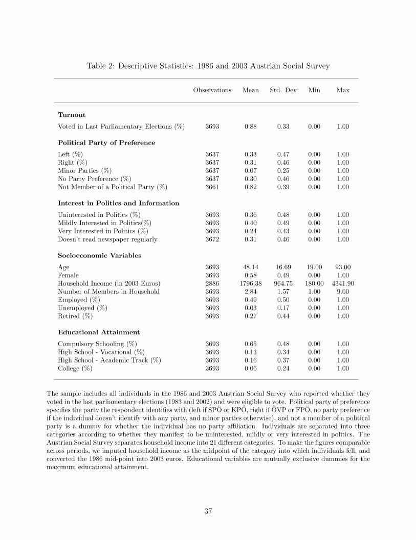
Table 2: Descriptive Statistics: 1986 and 2003 Austrian Social Survey

Observations Mean Std. Dev Min Max

Turnout

Voted in Last Parliamentary Elections (%) 3693 0.88 0.33 0.00 1.00

Political Party of Preference

Left (%) 3637 0.33 0.47 0.00 1.00Right (%) 3637 0.31 0.46 0.00 1.00Minor Parties (%) 3637 0.07 0.25 0.00 1.00No Party Preference (%) 3637 0.30 0.46 0.00 1.00Not Member of a Political Party (%) 3661 0.82 0.39 0.00 1.00

Interest in Politics and Information

Uninterested in Politics (%) 3693 0.36 0.48 0.00 1.00Mildly Interested in Politics(%) 3693 0.40 0.49 0.00 1.00Very Interested in Politics (%) 3693 0.24 0.43 0.00 1.00Doesn’t read newspaper regularly 3672 0.31 0.46 0.00 1.00

Socioeconomic Variables

Age 3693 48.14 16.69 19.00 93.00Female 3693 0.58 0.49 0.00 1.00Household Income (in 2003 Euros) 2886 1796.38 964.75 180.00 4341.90Number of Members in Household 3693 2.84 1.57 1.00 9.00Employed (%) 3693 0.49 0.50 0.00 1.00Unemployed (%) 3693 0.03 0.17 0.00 1.00Retired (%) 3693 0.27 0.44 0.00 1.00

Educational Attainment

Compulsory Schooling (%) 3693 0.65 0.48 0.00 1.00High School - Vocational (%) 3693 0.13 0.34 0.00 1.00High School - Academic Track (%) 3693 0.16 0.37 0.00 1.00College (%) 3693 0.06 0.24 0.00 1.00

The sample includes all individuals in the 1986 and 2003 Austrian Social Survey who reported whether theyvoted in the last parliamentary elections (1983 and 2002) and were eligible to vote. Political party of preferencespecifies the party the respondent identifies with (left if SPO or KPO, right if OVP or FPO, no party preferenceif the individual doesn’t identify with any party, and minor parties otherwise), and not a member of a politicalparty is a dummy for whether the individual has no party affiliation. Individuals are separated into threecategories according to whether they manifest to be uninterested, mildly or very interested in politics. TheAustrian Social Survey separates household income into 21 different categories. To make the figures comparableacross periods, we imputed household income as the midpoint of the category into which individuals fell, andconverted the 1986 mid-point into 2003 euros. Educational variables are mutually exclusive dummies for themaximum educational attainment.

37

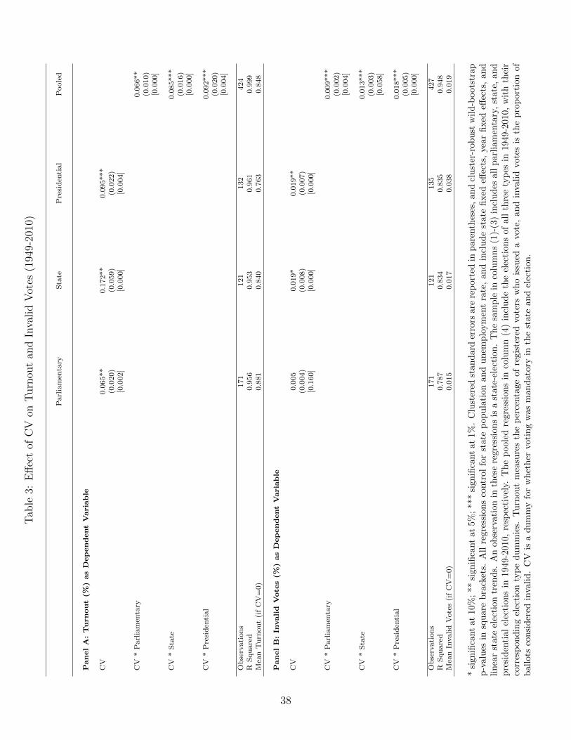
Tab

le3:

Eff

ect

ofC

Von

Turn

out

and

Inva

lid

Vot

es(1

949-

2010

)

Parliamen

tary

State

Presiden

tial

Pooled

PanelA:Turnout(%

)asDependentVariable

CV

0.065**

0.172**

0.095***

(0.020)

(0.059)

(0.022)

[0.002]

[0.000]

[0.004]

CV

*Parliamen

tary

0.066**

(0.010)

[0.000]

CV

*State

0.085***

(0.016)

[0.000]

CV

*Presiden

tial

0.092***

(0.020)

[0.004]

Observations

171

121

132

424

RSquared

0.956

0.953

0.961

0.999

Mea

nTurn

out(ifCV=0)

0.881

0.840

0.763

0.848

PanelB:In

valid

Vote

s(%

)asDependentVariable

CV

0.005

0.019*

0.019**

(0.004)

(0.008)

(0.007)

[0.160]

[0.000]

[0.000]

CV

*Parliamen

tary

0.009***

(0.002)

[0.004]

CV

*State

0.013***

(0.003)

[0.058]

CV

*Presiden

tial

0.018***

(0.005)

[0.000]

Observations

171

121

135

427

RSquared

0.787

0.834

0.835

0.948

Mea

nInvalidVotes(ifCV=0)

0.015

0.017

0.038

0.019

*si

gnifi

cant

at10

%;

**si

gnifi

cant

at5%

;**

*si

gnifi

cant

at

1%

.C

lust

ered

stan

dard

erro

rsare

rep

ort

edin

pare

nth

eses

,an

dcl

ust

er-r

ob

ust

wil

d-b

oots

trap

p-v

alu

esin

squ

are

bra

cket

s.A

llre

gres

sion

sco

ntr

ol

for

state

pop

ula

tion

an

du

nem

plo

ym

ent

rate

,an

din

clu

de

state

fixed

effec

ts,

yea

rfixed

effec

ts,

an

dli

nea

rst

ate

elec

tion

tren

ds.

An

obse

rvat

ion

inth

ese

regre

ssio

ns

isa

state

-ele

ctio

n.

Th

esa

mp

lein

colu

mn

s(1

)-(3

)in

clu

des

all

parl

iam

enta

ry,

state

,an

dp

resi

den

tial

elec

tion

sin

1949

-201

0,re

spec

tive

ly.

The

poole

dre

gre

ssio

ns

inco

lum

n(4

)in

clu

de

the

elec

tion

sof

all

thre

ety

pes

in1949-2

010,

wit

hth

eir

corr

esp

ond

ing

elec

tion

typ

ed

um

mie

s.T

urn

out

mea

sure

sth

ep

erce

nta

ge

of

regis

tere

dvote

rsw

ho

issu

eda

vote

,an

din

vali

dvo

tes

isth

ep

rop

ort

ion

of

bal

lots

con

sid

ered

inva

lid

.C

Vis

ad

um

my

for

wh

eth

ervo

tin

gw

as

man

dato

ryin

the

state

an

del

ecti

on

.

38

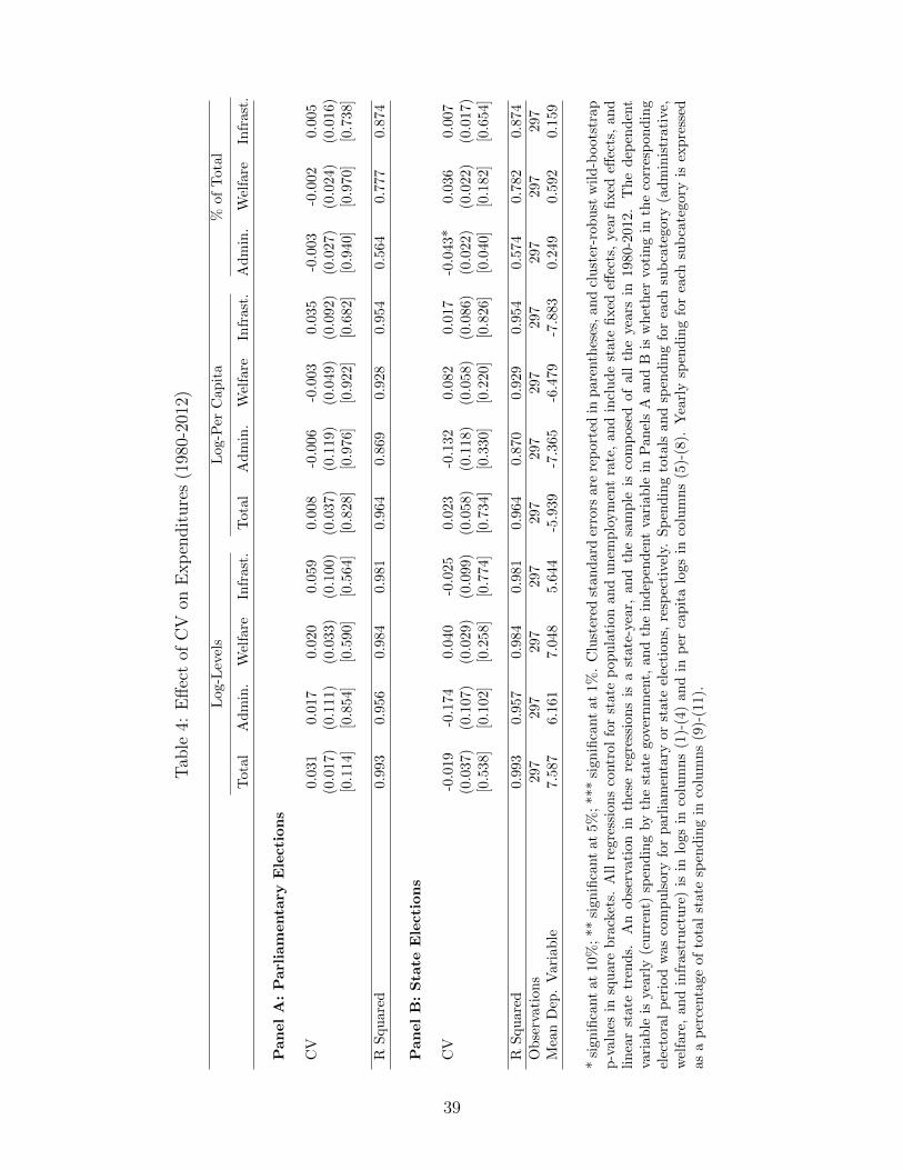
Tab

le4:

Eff

ect

ofC

Von

Exp

endit

ure

s(1

980-

2012

)

Log-L

evel

sL

og-P

erC

ap

ita

%of

Tota

l

Tot

alA

dm

in.

Wel

fare

Infr

ast

.T

ota

lA

dm

in.

Wel

fare

Infr

ast

.A

dm

in.

Wel

fare

Infr

ast

.

Pan

el

A:

Parl

iam

enta

ryE

lecti

on

s

CV

0.03

10.0

17

0.0

20

0.0

59

0.0

08

-0.0

06

-0.0

03

0.0

35

-0.0

03

-0.0

02

0.0

05

(0.0

17)

(0.1

11)

(0.0

33)

(0.1

00)

(0.0

37)

(0.1

19)

(0.0

49)

(0.0

92)

(0.0

27)

(0.0

24)

(0.0

16)

[0.1

14]

[0.8

54]

[0.5

90]

[0.5

64]

[0.8

28]

[0.9

76]

[0.9

22]

[0.6

82]

[0.9

40]

[0.9

70]

[0.7

38]

RS

qu

ared

0.99

30.9

56

0.9

84

0.9

81

0.9

64

0.8

69

0.9

28

0.9

54

0.5

64

0.7

77

0.8

74

Pan

el

B:

Sta

teE

lecti

on

s

CV

-0.0

19-0

.174

0.0

40

-0.0

25

0.0

23

-0.1

32

0.0

82

0.0

17

-0.0

43*

0.0

36

0.0

07

(0.0

37)

(0.1

07)

(0.0

29)

(0.0

99)

(0.0

58)

(0.1

18)

(0.0

58)

(0.0

86)

(0.0

22)

(0.0

22)

(0.0

17)

[0.5

38]

[0.1

02]

[0.2

58]

[0.7

74]

[0.7

34]

[0.3

30]

[0.2

20]

[0.8

26]

[0.0

40]

[0.1

82]

[0.6

54]

RS

qu

ared

0.99

30.9

57

0.9

84

0.9

81

0.9

64

0.8

70

0.9

29

0.9

54

0.5

74

0.7

82

0.8

74

Ob

serv

atio

ns

297

297

297

297

297

297

297

297

297

297

297

Mea

nD

ep.

Var

iab

le7.

587

6.1

61

7.0

48

5.6

44

-5.9

39

-7.3

65

-6.4

79

-7.8

83

0.2

49

0.5

92

0.1

59

*si

gnifi

cant

at10

%;

**si

gnifi

cant

at5%

;**

*si

gnifi

cant

at

1%

.C

lust

ered

stan

dard

erro

rsare

rep

ort

edin

pare

nth

eses

,an

dcl

ust

er-r

ob

ust

wil

d-b

oots

trap

p-v

alu

esin

squ

are

bra

cket

s.A

llre

gres

sion

sco

ntr

ol

for

state

pop

ula

tion

an

du

nem

plo

ym

ent

rate

,an

din

clu

de

state

fixed

effec

ts,

yea

rfixed

effec

ts,

an

dli

nea

rst

ate

tren

ds.

An

obse

rvat

ion

inth

ese

regre

ssio

ns

isa

state

-yea

r,an

dth

esa

mp

leis

com

pose

dof

all

the

years

in1980-2

012.

Th

ed

epen

den

tva

riab

leis

year

ly(c

urr

ent)

spen

din

gby

the

stat

egov

ernm

ent,

an

dth

ein

dep

enden

tva

riab

lein

Pan

els

Aan

dB

isw

het

her

voti

ng

inth

eco

rres

pon

din

gel

ecto

ral

per

iod

was

com

pu

lsor

yfo

rp

arli

amen

tary

or

state

elec

tion

s,re

spec

tivel

y.S

pen

din

gto

tals

an

dsp

end

ing

for

each

sub

cate

gory

(ad

min

istr

ati

ve,

wel

fare

,an

din

fras

tru

ctu

re)

isin

logs

inco

lum

ns

(1)-

(4)

an

din

per

cap

ita

logs

inco

lum

ns

(5)-

(8).

Yea

rly

spen

din

gfo

rea

chsu

bca

tegory

isex

pre

ssed

asa

per

centa

geof

tota

lst

ate

spen

din

gin

colu

mn

s(9

)-(1

1).

39

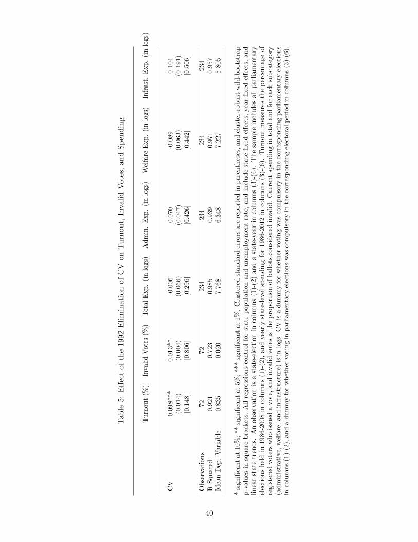
Tab

le5:

Eff

ect

ofth

e19

92E

lim

inat

ion

ofC

Von

Turn

out,

Inva

lid

Vot

es,

and

Sp

endin

g

Tu

rnou

t(%

)In

vali

dV

ote

s(%

)T

ota

lE

xp

.(i

nlo

gs)

Ad

min

.E

xp

.(i

nlo

gs)

Wel

fare

Exp

.(i

nlo

gs)

Infr

ast

.E

xp

.(i

nlo

gs)

CV

0.09

8***

0.01

3**

-0.0

06

0.0

70

-0.0

89

0.1

04

(0.0

14)

(0.0

04)

(0.0

66)

(0.0

47)

(0.0

63)

(0.1

91)

[0.1

48]

[0.8

06]

[0.2

96]

[0.4

26]

[0.4

42]

[0.5

06]

Ob

serv

atio

ns

7272

234

234

234

234

RS

qu

ared

0.92

10.

723

0.9

85

0.9

39

0.9

71

0.9

57

Mea

nD

ep.

Var

iab

le0.

835

0.02

07.7

68

6.3

48

7.2

27

5.8

05

*si

gnifi

cant

at10

%;

**si

gnifi

cant

at5%

;**

*si

gnifi

cant

at

1%

.C

lust

ered

stan

dard

erro

rsare

rep

ort

edin

pare

nth

eses

,an

dcl

ust

er-r

ob

ust

wil

d-b

oots

trap

p-v

alu

esin

squ

are

bra

cket

s.A

llre

gres

sion

sco

ntr

ol

for

state

pop

ula

tion

an

du

nem

plo

ym

ent

rate

,an

din

clu

de

state

fixed

effec

ts,

yea

rfixed

effec

ts,

an

dli

nea

rst

ate

tren

ds.

An

obse

rvat

ion

isa

stat

e-el

ecti

on

inco

lum

ns

(1)-

(2)

an

da

state

-yea

rin

colu

mn

s(3

)-(6

).T

he

sam

ple

incl

ud

esall

parl

iam

enta

ryel

ecti

ons

hel

din

1986

-200

8in

colu

mn

s(1

)-(2

),an

dye

arl

yst

ate

-lev

elsp

end

ing

for

1986-2

012

inco

lum

ns

(3)-

(6).

Tu

rnou

tm

easu

res

the

per

centa

ge

of

regi

ster

edvo

ters

wh

ois

sued

avo

te,

and

inva

lid

vote

sis

the

pro

port

ion

of

ball

ots

con

sid

ered

inva

lid

.C

urr

ent

spen

din

gin

tota

lan

dfo

rea

chsu

bca

tegory

(ad

min

istr

ativ

e,w

elfa

re,

and

infr

astr

uct

ure

)is

inlo

gs.

CV

isa

du

mm

yfo

rw

het

her

voti

ng

was

com

pu

lsory

inth

eco

rres

pon

din

gp

arl

iam

enta

ryel

ecti

on

sin

colu

mn

s(1

)-(2

),an

da

du

mm

yfo

rw

het

her

voti

ng

inp

arl

iam

enta

ryel

ecti

on

sw

as

com

pu

lsory

inth

eco

rres

pon

din

gel

ecto

ralp

erio

din

colu

mn

s(3

)-(6

).

40

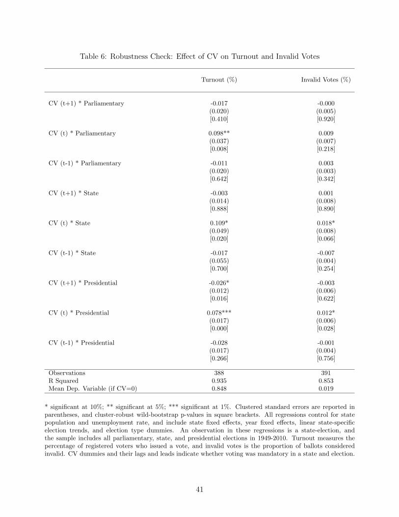
Table 6: Robustness Check: Effect of CV on Turnout and Invalid Votes

Turnout (%) Invalid Votes (%)

CV (t+1) * Parliamentary -0.017 -0.000(0.020) (0.005)[0.410] [0.920]

CV (t) * Parliamentary 0.098** 0.009(0.037) (0.007)[0.008] [0.218]

CV (t-1) * Parliamentary -0.011 0.003(0.020) (0.003)[0.642] [0.342]

CV (t+1) * State -0.003 0.001(0.014) (0.008)[0.888] [0.890]

CV (t) * State 0.109* 0.018*(0.049) (0.008)[0.020] [0.066]

CV (t-1) * State -0.017 -0.007(0.055) (0.004)[0.700] [0.254]

CV (t+1) * Presidential -0.026* -0.003(0.012) (0.006)[0.016] [0.622]

CV (t) * Presidential 0.078*** 0.012*(0.017) (0.006)[0.000] [0.028]

CV (t-1) * Presidential -0.028 -0.001(0.017) (0.004)[0.266] [0.756]

Observations 388 391R Squared 0.935 0.853Mean Dep. Variable (if CV=0) 0.848 0.019

* significant at 10%; ** significant at 5%; *** significant at 1%. Clustered standard errors are reported inparentheses, and cluster-robust wild-bootstrap p-values in square brackets. All regressions control for statepopulation and unemployment rate, and include state fixed effects, year fixed effects, linear state-specificelection trends, and election type dummies. An observation in these regressions is a state-election, andthe sample includes all parliamentary, state, and presidential elections in 1949-2010. Turnout measures thepercentage of registered voters who issued a vote, and invalid votes is the proportion of ballots consideredinvalid. CV dummies and their lags and leads indicate whether voting was mandatory in a state and election.

41

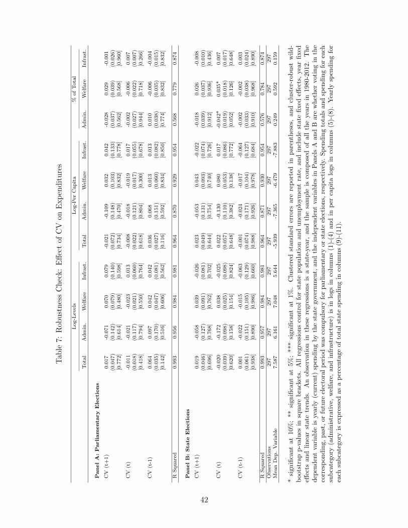
Tab

le7:

Rob

ust

nes

sC

hec

k:

Eff

ect

ofC

Von

Exp

endit

ure

s

Log-L

evels

Log-P

erCapita

%ofTotal

Total

Admin.

Welfare

Infrast.

Total

Admin.

Welfare

Infrast.

Admin.

Welfare

Infrast.

PanelA:Parliam

enta

ry

Elections

CV

(t+1)

0.017

-0.071

0.070

0.079

-0.021

-0.109

0.032

0.042

-0.028

0.029

-0.001

(0.047)

(0.142)

(0.079)

(0.140)

(0.072)

(0.148)

(0.103)

(0.133)

(0.037)

(0.039)

(0.026)

[0.772]

[0.614]

[0.480]

[0.598]

[0.734]

[0.470]

[0.832]

[0.778]

[0.562]

[0.568]

[0.960]

CV

(t)

-0.011

-0.021

-0.023

0.013

-0.008

-0.018

-0.019

0.017

-0.002

-0.006

0.007

(0.018)

(0.117)

(0.021)

(0.060)

(0.022)

(0.121)

(0.017)

(0.055)

(0.027)

(0.022)

(0.007)

[0.418]

[0.794]

[0.550]

[0.764]

[0.618]

[0.804]

[0.300]

[0.678]

[0.944]

[0.718]

[0.266]

CV

(t-1)

0.064

0.097

0.042

0.042

0.036

0.068

0.013

0.013

0.010

-0.006

-0.004

(0.035)

(0.170)

(0.047)

(0.081)

(0.027)

(0.151)

(0.060)

(0.082)

(0.038)

(0.035)

(0.015)

[0.142]

[0.516]

[0.606]

[0.562]

[0.116]

[0.592]

[0.834]

[0.850]

[0.774]

[0.832]

[0.832]

RSquared

0.993

0.956

0.984

0.981

0.964

0.870

0.929

0.954

0.568

0.779

0.874

PanelB:Sta

teElections

CV

(t+1)

0.019

-0.058

0.039

-0.026

0.023

-0.053

0.043

-0.022

-0.018

0.026

-0.008

(0.046)

(0.127)

(0.091)

(0.081)

(0.049)

(0.131)

(0.093)

(0.074)

(0.039)

(0.037)

(0.010)

[0.696]

[0.768]

[0.762]

[0.702]

[0.644]

[0.754]

[0.740]

[0.726]

[0.912]

[0.936]

[0.436]

CV

(t)

-0.020

-0.172

0.038

-0.025

0.022

-0.130

0.080

0.017

-0.042*

0.035*

0.007

(0.039)

(0.098)

(0.025)

(0.098)

(0.057)

(0.110)

(0.053)

(0.086)

(0.019)

(0.018)

(0.017)

[0.620]

[0.158]

[0.154]

[0.824]

[0.648]

[0.382]

[0.138]

[0.772]

[0.052]

[0.126]

[0.648]

CV

(t-1)

0.001

-0.022

-0.015

-0.063

-0.001

-0.024

-0.017

-0.064

-0.002

-0.002

0.003

(0.061)

(0.151)

(0.105)

(0.129)

(0.074)

(0.171)

(0.104)

(0.127)

(0.033)

(0.038)

(0.024)

[0.938]

[0.890]

[0.986]

[0.660]

[0.988]

[0.926]

[0.978]

[0.684]

[0.910]

[0.968]

[0.890]

RSquared

0.993

0.957

0.984

0.981

0.964

0.871

0.930

0.954

0.576

0.784

0.874

Observations

297

297

297

297

297

297

297

297

297

297

297

Mea

nDep

.Variable

7.587

6.161

7.048

5.644

-5.939

-7.365

-6.479

-7.883

0.249

0.592

0.159

*si

gnifi

cant

at10

%;

**si

gnifi

cant

at5%

;**

*si

gn

ifica

nt

at

1%

.C

lust

ered

stan

dard

erro

rsare

rep

ort

edin

pare

nth

eses

,an

dcl

ust

er-r

ob

ust

wil

d-

boot

stra

pp

-val

ues

insq

uar

eb

rack

ets.

All

regr

essi

on

sco

ntr

ol

for

state

pop

ula

tion

an

du

nem

plo

ym

ent

rate

,an

din

clu

de

state

fixed

effec

ts,

yea

rfixed

effec

tsan

dli

nea

rst

ate

tren

ds.

An

obse

rvat

ion

inth

ese

regre

ssio

ns

isa

state

-yea

r,an

dth

esa

mp

leis

com

pose

dof

all

the

years

in1980-2

012.

Th

ed

epen

den

tva

riab

leis

year

ly(c

urr

ent)

spen

din

gby

the

state

gov

ern

men

t,an

dth

ein

dep

end

ent

vari

ab

les

inP

an

els

Aan

dB

are

wh

eth

ervo

tin

gin

the

corr

esp

ond

ing,

pas

t,or

futu

reel

ecto

ral

per

iod

was

com

pu

lsory

for

parl

iam

enta

ryor

state

elec

tion

s,re

spec

tive

ly.

Sp

end

ing

tota

lsan

dsp

end

ing

for

each

sub

cate

gory

(ad

min

istr

ativ

e,w

elfa

re,

and

infr

astr

uct

ure

)is

inlo

gs

inco

lum

ns

(1)-

(4)

an

din

per

cap

ita

logs

inco

lum

ns

(5)-

(8).

Yea

rly

spen

din

gfo

rea

chsu

bca

tego

ryis

exp

ress

edas

ap

erce

nta

geof

tota

lst

ate

spen

din

gin

colu

mn

s(9

)-(1

1).

42

Tab

le8:

Eff

ect

ofC

Von

Pol

itic

alC

omp

etit

ion

(194

9-20

10)

Lef

t(%

)R

ight

(%)

Nu

m.

of

Part

ies

Sh

are

Win

ner

(%)

Marg

inof

Vic

tory

Pan

el

A:

Parl

iam

enta

ryE

lecti

on

s

CV

-0.0

14

0.0

14

0.4

28

0.0

15

0.0

29

(0.0

10)

(0.0

17)

(0.3

37)

(0.0

18)

(0.0

25)

[0.1

02]

[0.4

24]

[0.3

14]

[0.2

64]

[0.1

02]

Ob

serv

atio

ns

171

171

171

171

171

RS

qu

ared

0.9

84

0.9

24

0.9

67

0.8

89

0.7

68

Mea

nD

ep.

Var

iab

le0.4

00

0.5

15

6.9

59

0.4

65

0.1

20

Pan

el

B:

Sta

teE

lecti

on

s

CV

0.0

35

0.0

01

-0.0

51

0.0

14

0.0

04

(0.0

46)

(0.0

38)

(0.5

14)

(0.0

36)

(0.0

44)

[0.5

90]

[0.9

92]

[0.8

62]

[0.6

28]

[0.9

50]

Ob

serv

atio

ns

121

121

121

121

121

RS

qu

ared

0.9

67

0.9

15

0.8

23

0.8

70

0.7

90

Mea

nD

ep.

Var

iab

le0.3

93

0.5

35

5.9

75

0.4

94

0.1

01

*si

gnifi

cant

at10

%;

**si

gnifi

cant

at5%

;**

*si

gnifi

cant

at

1%

.C

lust

ered

stan

dard

erro

rsare

rep

ort

edin

pare

nth

eses

,an

dcl

ust

er-r

ob

ust

wil

d-b

oots

trap

p-v

alu

esin

squ

are

bra

cket

s.A

llre

gres

sion

sco

ntr

ol

for

state

pop

ula

tion

an

du

nem

plo

ym

ent

rate

,an

din

clu

de

state

fixed

effec

ts,

yea

rfixed

effec

ts,

an

dli

nea

rst

ate

elec

tion

tren

ds.

An

obse

rvat

ion

inth

ese

regre

ssio

ns

isa

state

-ele

ctio

n.

Th

esa

mple

inP

an

els

Aan

dB

incl

ud

esall

parl

iam

enta

ryan

dst

ate

elec

tion

sin

1949

-201

0,re

spec

tive

ly.

Vot

esh

ares

for

the

left

and

right

are

the

per

centa

ge

of

vali

dvo

tes

that

wen

tto

SP

O+

KP

Oan

dO

VP

+F

PO

,re

spec

tive

ly.

Num

ber

ofp

arti

esis

the

nu

mb

erof

part

ies

part

icip

ati

ng

inea

chel

ecti

on

an

dst

ate

.T

he

vote

share

of

the

win

ner

isth

ep

erce

nta

ge

of

vali

dvo

tes

obta

ined

by

the

hig

hes

tra

nkin

gp

arty

inea

chst

ate

,an

dm

arg

inof

vic

tory

isth

ediff

eren

cein

vote

share

sb

etw

een

the

hig

hes

tra

nkin

gp

art

yan

dth

eru

nn

er-u

p.

CV

isa

du

mm

yfo

rw

het

her

voti

ng

was

man

dato

ryin

the

state

inth

at

part

icu

lar

elec

tion

.

43

Table 9: Effect of CV on Voter Composition

Dependent Variable: Voted in Last Parliamentary Elections

1) Effect of CV on Turnout

CV 0.058**(0.023)

2) Gender

Female * CV 0.055**(0.027)

3) Educational Attainment

Compulsory Schooling * CV 0.060**(0.024)

Vocational High School * CV 0.050(0.042)

Academic High School or College * CV 0.059(0.036)

4) Income Quartile

Income Q1 * CV 0.060*(0.035)

Income Q2 * CV 0.069**(0.035)

Income Q3 * CV 0.032(0.037)

Income Q4 * CV 0.035(0.040)

Observations 3,440 3,440 3,440 2,682R Squared 0.093 0.093 0.888 0.895

* significant at 10%; ** significant at 5%; *** significant at 1%. Robust standard errors reported in parentheses.All regressions control for age, age squared, gender, educational attainment, parents’ education, workingstatus, household size, community size, state fixed effects, and survey year fixed effects. The sample includesall individuals in the 1986 and 2003 Austrian Social Survey who reported whether they voted in the lastparliamentary elections (1983 and 2002) and were eligible to vote. The dependent variable in all regressionsis a dummy for whether the individual voted in the previous parliamentary elections, and CV is a dummy forwhether voting was compulsory for that election in the individual’s state of residence. Regression in Panel2 includes compulsory voting and female dummies, but we only report their interaction. For regression 3 weseparated individuals into three educational categories according to their maximum educational attainment.For regression 4 we calculated individual’s equalized income by dividing the mid-point of the category in whichtheir household income fell with respect to the equalized household size, and separated the survey respondentsinto quartiles for each wave. Regressions in Panels 3)-4) omit the constant, and include the full set of schoolingand income quartile dummies, although we only report the interaction terms.

44

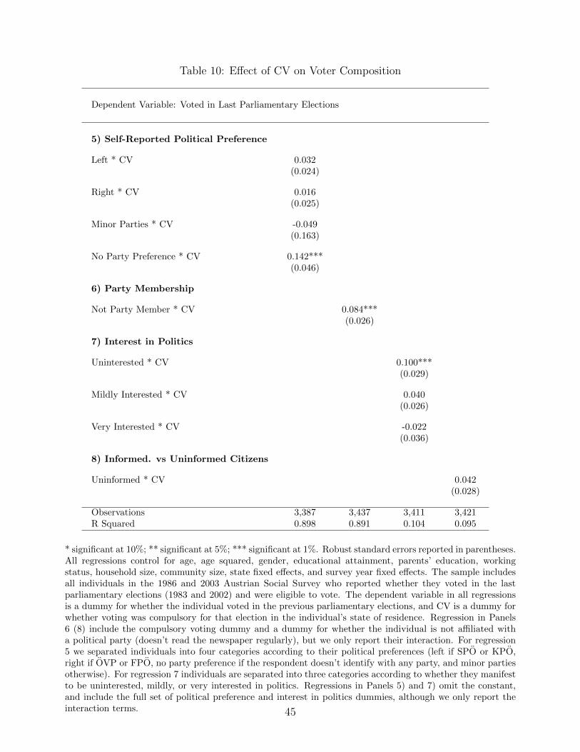
Table 10: Effect of CV on Voter Composition

Dependent Variable: Voted in Last Parliamentary Elections

5) Self-Reported Political Preference

Left * CV 0.032(0.024)

Right * CV 0.016(0.025)

Minor Parties * CV -0.049(0.163)

No Party Preference * CV 0.142***(0.046)

6) Party Membership

Not Party Member * CV 0.084***(0.026)

7) Interest in Politics

Uninterested * CV 0.100***(0.029)

Mildly Interested * CV 0.040(0.026)

Very Interested * CV -0.022(0.036)

8) Informed. vs Uninformed Citizens

Uninformed * CV 0.042(0.028)

Observations 3,387 3,437 3,411 3,421R Squared 0.898 0.891 0.104 0.095

* significant at 10%; ** significant at 5%; *** significant at 1%. Robust standard errors reported in parentheses.All regressions control for age, age squared, gender, educational attainment, parents’ education, workingstatus, household size, community size, state fixed effects, and survey year fixed effects. The sample includesall individuals in the 1986 and 2003 Austrian Social Survey who reported whether they voted in the lastparliamentary elections (1983 and 2002) and were eligible to vote. The dependent variable in all regressionsis a dummy for whether the individual voted in the previous parliamentary elections, and CV is a dummy forwhether voting was compulsory for that election in the individual’s state of residence. Regression in Panels6 (8) include the compulsory voting dummy and a dummy for whether the individual is not affiliated witha political party (doesn’t read the newspaper regularly), but we only report their interaction. For regression5 we separated individuals into four categories according to their political preferences (left if SPO or KPO,right if OVP or FPO, no party preference if the respondent doesn’t identify with any party, and minor partiesotherwise). For regression 7 individuals are separated into three categories according to whether they manifestto be uninterested, mildly, or very interested in politics. Regressions in Panels 5) and 7) omit the constant,and include the full set of political preference and interest in politics dummies, although we only report theinteraction terms. 45

Appendix A Tables (Not intended for publication)

46

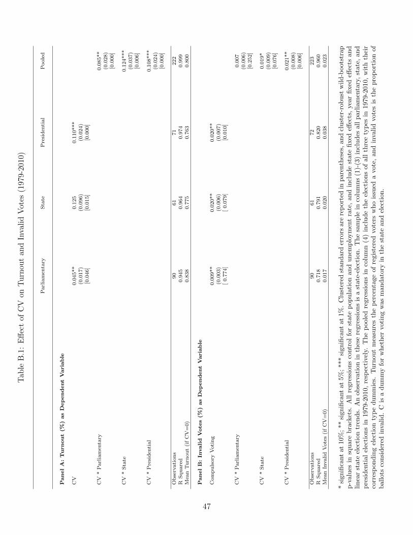
Tab

leB

.1:

Eff

ect

ofC

Von

Turn

out

and

Inva

lid

Vot

es(1

979-

2010

)

Parliamen

tary

State

Presiden

tial

Pooled

PanelA:Turnout(%

)asDependentVariable

CV

0.045**

0.125

0.110***

(0.017)

(0.096)

(0.024)

[0.046]

[0.015]

[0.000]

CV

*Parliamen

tary

0.085**

(0.028)

[0.000]

CV

*State

0.124***

(0.037)

[0.006]

CV

*Presiden

tial

0.108***

(0.024)

[0.000]

Observations

90

61

71

222

RSquared

0.945

0.964

0.974

0.999

Mea

nTurn

out(ifCV=0)

0.838

0.775

0.763

0.800

PanelB:In

valid

Vote

s(%

)asDependentVariable

Compulsory

Voting

0.009**

0.020**

0.020**

(0.003)

(0.006)

(0.007)

[0.774]

[0.079]

[0.010]

CV

*Parliamen

tary

0.007

(0.006)

[0.252]

CV

*State

0.019*

(0.009)

[0.076]

CV

*Presiden

tial

0.021**

(0.008)

[0.006]

Observations

90

61

72

223

RSquared

0.718

0.791

0.820

0.960

Mea

nInvalidVotes(ifCV=0)

0.017

0.020

0.038

0.023

*si

gnifi

cant

at10

%;

**si

gnifi

cant

at5%

;**

*si

gnifi

cant

at

1%

.C

lust

ered

stan

dard

erro

rsare

rep

ort

edin

pare

nth

eses

,an

dcl

ust

er-r

ob

ust

wil

d-b

oots

trap

p-v

alu

esin

squ

are

bra

cket

s.A

llre

gres

sion

sco

ntr

ol

for

state

pop

ula

tion

an

du

nem

plo

ym

ent

rate

,an

din

clu

de

state

fixed

effec

ts,

year

fixed

effec

tsan

dli

nea

rst

ate

elec

tion

tren

ds.

An

obse

rvat

ion

inth

ese

regre

ssio

ns

isa

state

-ele

ctio

n.

Th

esa

mp

lein

colu

mn

s(1

)-(3

)in

clu

des

all

parl

iam

enta

ry,

state

,an

dp

resi

den

tial

elec

tion

sin

1979

-201

0,re

spec

tive

ly.

The

poole

dre

gre

ssio

ns

inco

lum

n(4

)in

clu

de

the

elec

tion

sof

all

thre

ety

pes

in1979-2

010,

wit

hth

eir

corr

esp

ond

ing

elec

tion

typ

ed

um

mie

s.T

urn

out

mea

sure

sth

ep

erce

nta

ge

of

regis

tere

dvote

rsw

ho

issu

eda

vote

,an

din

vali

dvo

tes

isth

ep

rop

ort

ion

of

bal

lots

con

sid

ered

inva

lid

.C

isa

du

mm

yfo

rw

het

her

voti

ng

was

man

dato

ryin

the

state

an

del

ecti

on

.

47

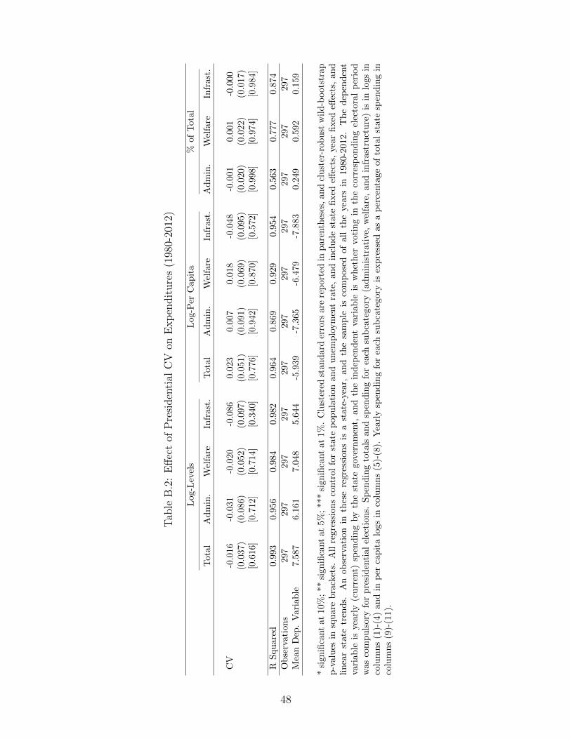
Tab

leB

.2:

Eff

ect

ofP

resi

den

tial

CV

onE

xp

endit

ure

s(1

980-

2012

)

Log

-Lev

els

Log-P

erC

ap

ita

%of

Tota

l

Tot

alA

dm

in.

Wel

fare

Infr

ast

.T

ota

lA

dm

in.

Wel

fare

Infr

ast

.A

dm

in.

Wel

fare

Infr

ast

.

CV

-0.0

16-0

.031

-0.0

20

-0.0

86

0.0

23

0.0

07

0.0

18

-0.0

48

-0.0

01

0.0

01

-0.0

00

(0.0

37)

(0.0

86)

(0.0

52)

(0.0

97)

(0.0

51)

(0.0

91)

(0.0

69)

(0.0

95)

(0.0

20)

(0.0

22)

(0.0

17)

[0.6

16]

[0.7

12]

[0.7

14]

[0.3

40]

[0.7

76]

[0.9

42]

[0.8

70]

[0.5

72]

[0.9

98]

[0.9

74]

[0.9

84]

RS

qu

ared

0.99

30.

956

0.9

84

0.9

82

0.9

64

0.8

69

0.9

29

0.9

54

0.5

63

0.7

77

0.8

74

Ob

serv

atio

ns

297

297

297

297

297

297

297

297

297

297

297

Mea

nD

ep.

Var

iab

le7.

587

6.16

17.0

48

5.6

44

-5.9

39

-7.3

65

-6.4

79

-7.8

83

0.2

49

0.5

92

0.1

59

*si

gnifi

cant

at10

%;

**si

gnifi

cant

at5%

;**

*si

gnifi

cant

at

1%

.C

lust

ered

stan

dard

erro

rsare

rep

ort

edin

pare

nth

eses

,an

dcl

ust

er-r

ob

ust

wil

d-b

oots

trap

p-v

alu

esin

squ

are

bra

cket

s.A

llre

gres

sion

sco

ntr

ol

for

state

pop

ula

tion

an

du

nem

plo

ym

ent

rate

,an

din

clu

de

state

fixed

effec

ts,

yea

rfixed

effec

ts,

an

dli

nea

rst

ate

tren

ds.

An

obse

rvat

ion

inth

ese

regre

ssio

ns

isa

state

-yea

r,an

dth

esa

mp

leis

com

pose

dof

all

the

years

in1980-2

012.

Th

ed

epen

den

tva

riab

leis

year

ly(c

urr

ent)

spen

din

gby

the

state

gov

ern

men

t,an

dth

ein

dep

end

ent

vari

ab

leis

wh

eth

ervo

tin

gin

the

corr

esp

ond

ing

elec

tora

lp

erio

dw

asco

mp

uls

ory

for

pre

sid

enti

alel

ecti

ons.

Sp

end

ing

tota

lsan

dsp

end

ing

for

each

sub

cate

gory

(ad

min

istr

ati

ve,

wel

fare

,an

din

frast

ruct

ure

)is

inlo

gs

inco

lum

ns

(1)-

(4)

and

inp

erca

pit

alo

gsin

colu

mn

s(5

)-(8

).Y

earl

ysp

end

ing

for

each

sub

cate

gory

isex

pre

ssed

as

ap

erce

nta

ge

of

tota

lst

ate

spen

din

gin

colu

mn

s(9

)-(1

1).

48

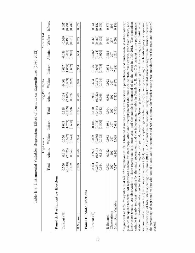
Tab

leB

.3:

Inst

rum

enta

lV

aria

ble

sR

egre

ssio

n:

Eff

ect

ofT

urn

out

onE

xp

endit

ure

s(1

980-

2012

)

Log-L

evel

sL

og-P

erC

ap

ita

%of

Tota

l

Tot

alA

dm

in.

Wel

fare

Infr

ast

.T

ota

lA

dm

in.

Wel

fare

Infr

ast

.A

dm

in.

Wel

fare

Infr

ast

.

Pan

el

A:

Parl

iam

enta

ryE

lecti

on

s

Tu

rnou

t(%

)0.

556

0.3

10

0.3

56

1.0

45

0.1

38

-0.1

08

-0.0

62

0.6

27

-0.0

58

-0.0

29

0.0

87

(0.4

48)

(2.0

25)

(0.5

92)

(1.7

59)

(0.7

03)

(2.1

03)

(0.8

63)

(1.6

58)

(0.4

69)

(0.4

30)

(0.2

91)

[0.1

82]

[0.8

54]

[0.5

74]

[0.5

58]

[0.8

36]

[0.9

76]

[0.9

22]

[0.6

82]

[0.9

40]

[0.9

70]

[0.7

32]

RS

qu

ared

0.99

30.9

56

0.9

84

0.9

81

0.9

64

0.8

69

0.9

28

0.9

54

0.5

64

0.7

77

0.8

74

Pan

el

B:

Sta

teE

lecti

on

s

Tu

rnou

t(%

)-0

.141

-1.2

77

0.2

92

-0.1

86

0.1

70

-0.9

66

0.6

03

0.1

26

-0.3

15*

0.2

63

0.0

51

(0.2

61)

(0.8

11)

(0.2

36)

(0.7

02)

(0.4

14)

(0.9

32)

(0.3

77)

(0.6

36)

(0.1

74)

(0.1

69)

(0.1

27)

[0.6

34]

[0.1

10]

[0.1

92]

[0.8

00]

[0.6

42]

[0.3

66]

[0.1

64]

[0.7

68]

[0.0

76]

[0.1

32]

[0.6

56]

RS

qu

ared

0.99

30.9

52

0.9

83

0.9

81

0.9

64

0.8

61

0.9

23

0.9

54

0.5

13

0.7

50

0.8

73

Ob

serv

atio

ns

297

297

297

297

297

297

297

297

297

297

297

Mea

nD

ep.

Var

iab

le7.

587

6.1

61

7.0

48

5.6

44

-5.9

39

-7.3

65

-6.4

79

-7.8

83

0.2

49

0.5

92

0.1

59

*si

gnifi

cant

at10

%;

**si

gnifi

cant

at5%

;**

*si

gnifi

cant

at

1%

.C

lust

ered

stan

dard

erro

rsare

rep

ort

edin

pare

nth

eses

,an

dcl

ust

er-r

ob

ust

wil

d-b

oots

trap

p-v

alu

esin

squ

are

bra

cket

s.A

llre

gres

sion

sco

ntr

ol

for

state

pop

ula

tion

an

du

nem

plo

ym

ent

rate

,an

din

clu

de

state

fixed

effec

ts,

yea

rfixed

effec

ts,

an

dli

nea

rst

ate

tren

ds.

An

obse

rvat

ion

inth

ese

regre

ssio

ns

isa

state

-yea

r,an

dth

esa

mp

leis

com

pose

dof

all

the

years

in1980-2

012.

Th

ed

epen

den

tva

riab

leis

year

ly(c

urr

ent)

spen

din

gby

the

stat

egov

ern

men

t,an

dth

ein

dep

end

ent

vari

ab

lein

Pan

els

A,

B,

an

dC

istu

rnou

tin

the

parl

iam

enta

ry,

stat

e,an

dp

resi

den

tial

elec

tion

sfo

rth

eco

rres

pon

din

gel

ecto

ral

per

iod

,re

spec

tive

ly.

Sp

end

ing

tota

lsan

dsp

end

ing

for

each

sub

cate

gory

(ad

min

istr

ati

ve,

wel

fare

,an

din

fras

tru

ctu

re)

isin

logs

inco

lum

ns

(1)-

(4)

an

din

per

cap

ita

logs

inco

lum

ns

(5)-

(8).

Yea

rly

spen

din

gfo

rea

chsu

bca

tegory

isex

pre

ssed

asa

per

centa

geof

tota

lst

ate

spen

din

gin

colu

mn

s(9

)-(1

1).

All

equ

ati

on

sare

esti

mate

du

sin

gan

inst

rum

enta

lva

riab

les

regre

ssio

n.

Tu

rnou

tm

easu

res

the

per

centa

geof

regi

ster

edvo

ters

wh

ois

sued

avo

te,

an

dis

inst

rum

ente

dw

ith

ad

um

my

for

wh

eth

ervo

tin

gw

as

man

dato

ryin

the

state

an

del

ecto

ral

per

iod.

49

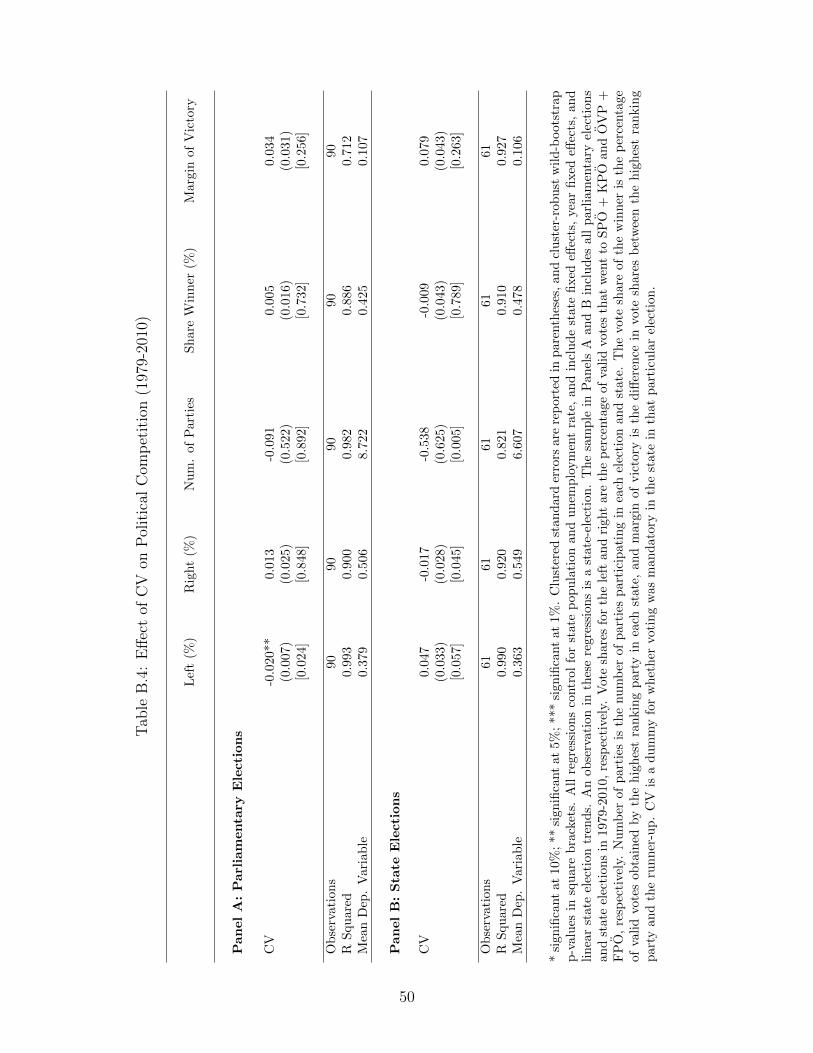
Tab

leB

.4:

Eff

ect

ofC

Von

Pol

itic

alC

omp

etit

ion

(197

9-20

10)

Lef

t(%

)R

ight

(%)

Nu

m.

of

Part

ies

Sh

are

Win

ner

(%)

Marg

inof

Vic

tory

Pan

el

A:

Parl

iam

enta

ryE

lecti

on

s

CV

-0.0

20**

0.0

13

-0.0

91

0.0

05

0.0

34

(0.0

07)

(0.0

25)

(0.5

22)

(0.0

16)

(0.0

31)

[0.0

24]

[0.8

48]

[0.8

92]

[0.7

32]

[0.2

56]

Ob

serv

atio

ns

90

90

90

90

90

RS

qu

ared

0.9

93

0.9

00

0.9

82

0.8

86

0.7

12

Mea

nD

ep.

Var

iab

le0.3

79

0.5

06

8.7

22

0.4

25

0.1

07

Pan

el

B:

Sta

teE

lecti

on

s

CV

0.0

47

-0.0

17

-0.5

38

-0.0

09

0.0

79

(0.0

33)

(0.0

28)

(0.6

25)

(0.0

43)

(0.0

43)

[0.0

57]

[0.0

45]

[0.0

05]

[0.7

89]

[0.2

63]

Ob

serv

atio

ns

61

61

61

61

61

RS

qu

ared

0.9

90

0.9

20

0.8

21

0.9

10

0.9

27

Mea

nD

ep.

Var

iab

le0.3

63

0.5

49

6.6

07

0.4

78

0.1

06

*si

gnifi

cant

at10

%;

**si

gnifi

cant

at5%

;**

*si

gnifi

cant

at

1%

.C

lust

ered

stan

dard

erro

rsare

rep

ort

edin

pare

nth

eses

,an

dcl

ust

er-r

ob

ust

wil

d-b

oots

trap

p-v

alu

esin

squ

are

bra

cket

s.A

llre

gres

sion

sco

ntr

ol

for

state

pop

ula

tion

an

du

nem

plo

ym

ent

rate

,an

din

clu

de

state

fixed

effec

ts,

yea

rfixed

effec

ts,

an

dli

nea

rst

ate

elec

tion

tren

ds.

An

obse

rvat

ion

inth

ese

regre

ssio

ns

isa

state

-ele

ctio

n.

Th

esa

mp

lein

Pan

els

Aan

dB

incl

ud

esall

parl

iam

enta

ryel

ecti

on

san

dst

ate

elec

tion

sin

1979

-201

0,re

spec

tive

ly.

Vot

esh

are

sfo

rth

ele

ftan

dri

ght

are

the

per

centa

ge

of

vali

dvote

sth

at

wen

tto

SP

O+

KP

Oan

dO

VP

+F

PO

,re

spec

tivel

y.N

um

ber

ofp

arti

esis

the

nu

mb

erof

part

ies

part

icip

ati

ng

inea

chel

ecti

on

an

dst

ate

.T

he

vote

share

of

the

win

ner

isth

ep

erce

nta

ge

ofva

lid

vot

esob

tain

edby

the

hig

hes

tra

nkin

gp

arty

inea

chst

ate

,an

dm

arg

inof

vic

tory

isth

ed

iffer

ence

invo

tesh

are

sb

etw

een

the

hig

hes

tra

nkin

gp

arty

and

the

run

ner

-up

.C

Vis

ad

um

my

for

wh

eth

ervoti

ng

was

man

dato

ryin

the

state

inth

at

part

icu

lar

elec

tion

.

50

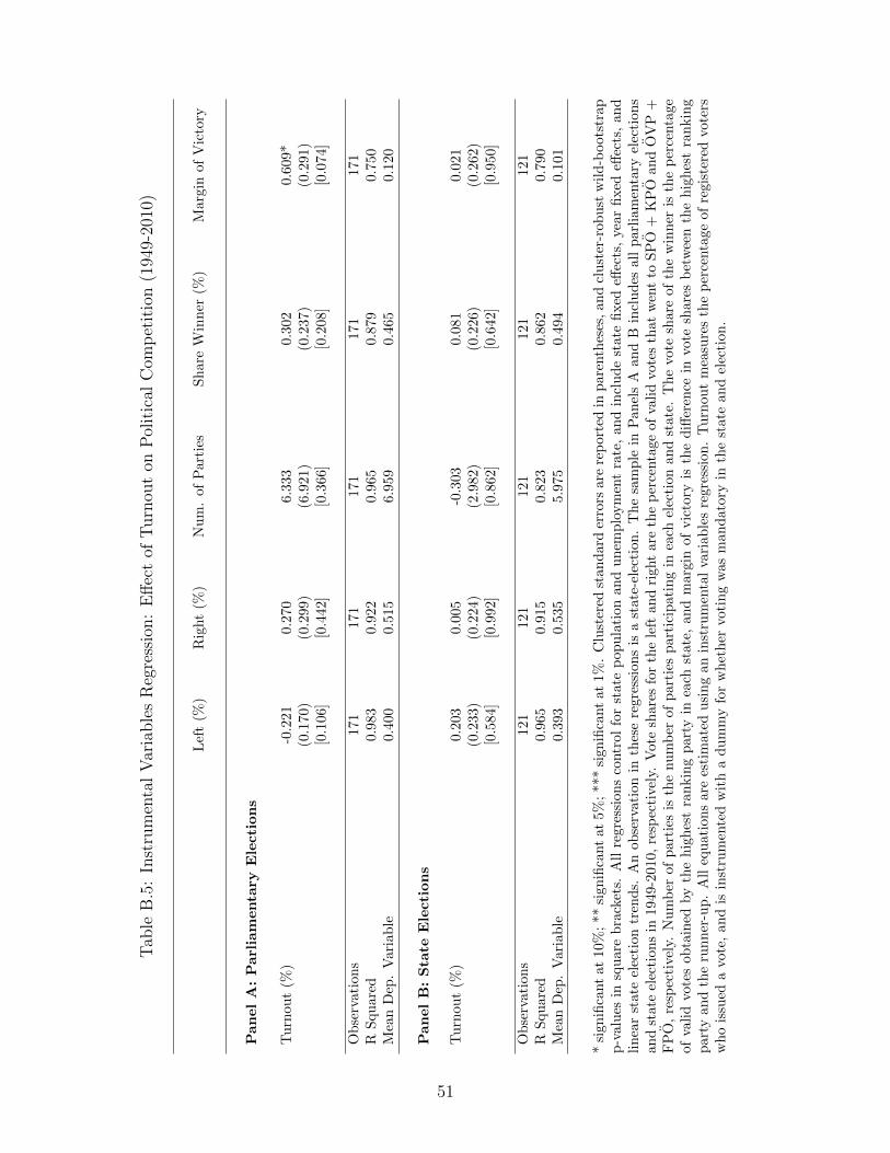
Tab

leB

.5:

Inst

rum

enta

lV

aria

ble

sR

egre

ssio

n:

Eff

ect

ofT

urn

out

onP

olit

ical

Com

pet

itio

n(1

949-

2010

)

Lef

t(%

)R

ight

(%)

Nu

m.

of

Part

ies

Sh

are

Win

ner

(%)

Marg

inof

Vic

tory

Pan

el

A:

Parl

iam

enta

ryE

lecti

on

s

Tu

rnou

t(%

)-0

.221

0.2

70

6.3

33

0.3

02

0.6

09*

(0.1

70)

(0.2

99)

(6.9

21)

(0.2

37)

(0.2

91)

[0.1

06]

[0.4

42]

[0.3

66]

[0.2

08]

[0.0

74]

Ob

serv

atio

ns

171

171

171

171

171

RS

qu

ared

0.9

83

0.9

22

0.9

65

0.8

79

0.7

50

Mea

nD

ep.

Var

iab

le0.4

00

0.5

15

6.9

59

0.4

65

0.1

20

Pan

el

B:

Sta

teE

lecti

on

s

Tu

rnou

t(%

)0.2

03

0.0

05

-0.3

03

0.0

81

0.0

21

(0.2

33)

(0.2

24)

(2.9

82)

(0.2

26)

(0.2

62)

[0.5

84]

[0.9

92]

[0.8

62]

[0.6

42]

[0.9

50]

Ob

serv

atio

ns

121

121

121

121

121

RS

qu

ared

0.9

65

0.9

15

0.8

23

0.8

62

0.7

90

Mea

nD

ep.

Var

iab

le0.3

93

0.5

35

5.9

75

0.4

94

0.1

01

*si

gnifi

cant

at10

%;

**si

gnifi

cant

at5%

;**

*si

gnifi

cant

at

1%

.C

lust

ered

stan

dard

erro

rsare

rep

ort

edin

pare

nth

eses

,an

dcl

ust

er-r

ob

ust

wil

d-b

oots

trap

p-v

alu

esin

squ

are

bra

cket

s.A

llre

gres

sion

sco

ntr

ol

for

state

pop

ula

tion

an

du

nem

plo

ym

ent

rate

,an

din

clu

de

state

fixed

effec

ts,

yea

rfixed

effec

ts,

an

dli

nea

rst

ate

elec

tion

tren

ds.

An

obse

rvat

ion

inth

ese

regre

ssio

ns

isa

state

-ele

ctio

n.

Th

esa

mp

lein

Pan

els

Aan

dB

incl

ud

esall

parl

iam

enta

ryel

ecti

on

san

dst

ate

elec

tion

sin

1949

-201

0,re

spec

tive

ly.

Vot

esh

are

sfo

rth

ele

ftan

dri

ght

are

the

per

centa

ge

of

vali

dvote

sth

at

wen

tto

SP

O+

KP

Oan

dO

VP

+F

PO

,re

spec

tivel

y.N

um

ber

ofp

arti

esis

the

nu

mb

erof

part

ies

part

icip

ati

ng

inea

chel

ecti

on

an

dst

ate

.T

he

vote

share

of

the

win

ner

isth

ep

erce

nta

ge

ofva

lid

vot

esob

tain

edby

the

hig

hes

tra

nkin

gp

arty

inea

chst

ate

,an

dm

arg

inof

vic

tory

isth

ed

iffer

ence

invo

tesh

are

sb

etw

een

the

hig

hes

tra

nkin

gp

arty

and

the

run

ner

-up

.A

lleq

uat

ion

sar

ees

tim

ate

du

sin

gan

inst

rum

enta

lva

riab

les

regre

ssio

n.

Tu

rnou

tm

easu

res

the

per

centa

ge

of

regis

tere

dvo

ters

wh

ois

sued

avo

te,

and

isin

stru

men

ted

wit

ha

du

mm

yfo

rw

het

her

voti

ng

was

man

dato

ryin

the

state

an

del

ecti

on

.

51

Appendix B Compulsory voting in Austria in the pre-

war period

The debate concerning the introduction of CV in Austria goes back to the enfranchisement

of women in 1918. Conservative parties feared that their women supporters would not be as

politically active and easy to mobilize as women who supported the social democrats, who had

advocated for universal voting rights in the first place. CV was therefore seen as an instrument

for conserving their power. Informal accounts mention that during the debates regarding the

implementation of CV, conservatives put forward the argument that participation in political

decisions and public life was not only a right but a duty of every citizen.48 Social democrats

were against its implementation, and thus a compromise was reached, leaving the prerogative

of instating mandatory voting to the states. In 1919, before the elections for the Constituent

National Assembly, provisions for CV were made in Vorarlberg and Tyrol.49 When the 1920

constitution was amended in December 1929, it became up to each state to decide whether

voting was compulsory or not in national parliament and state parliament elections.50

The 1920 constitution, which was parliamentary in nature, underwent other important

changes in 1929. The responsibilities of the president were broadened, and the election of

the president became determined by popular vote rather than by decision of the members of

the legislature. Furthermore, voting in presidential elections became mandatory in the whole

country.51 Although the first election was supposed to occur in 1931, due to the worldwide

economic depression, political parties decided to suspend the elections and reelect the incum-

bent president. In May 1934, the fascist ruling party repealed the 1929 constitution, but

after WWII, in May 1945, the 1920 constitution (with its 1929 amendments) was reinstated.

Thus, both the country-wide provisions for mandatory voting in presidential elections and the

state-determined CV in national parliament and state parliament elections were restored. In

48http://www.onb.ac.at/ariadne/projekte/frauenwaehlet/Raum07.html, last accessed April 19, 201549http://www.parlament.gv.at/PERK/HIS/WAHL/REGEL/index.shtml, last accessed April 19, 2015.50Federal Constitution of December 1929 (B-VG) Articles 26 (1) and 95 (1)-(2).51Federal Constitution of December 1929 (B-VG) Article 60 (1).

52

spite of this, and probably due to the post-war chaos, the 1945 national and state parliament

elections were carried out according to a national law made specifically for this election.52

Thus, voting in the 1945 elections was optional for individuals in all states, including Tyrol

and Vorarlberg. Only in the next election for national and state parliament, both held in 1949,

did Vorarlberg and Tyrol re-implement CV. Furthermore, the state of Styria also enacted its

own CV law for these elections.53

52Election Law 198 (Wahlgesetz) from October 1945.53Styria Law 30 from July 11, 1949.

53