Embed Size (px)
Citation preview
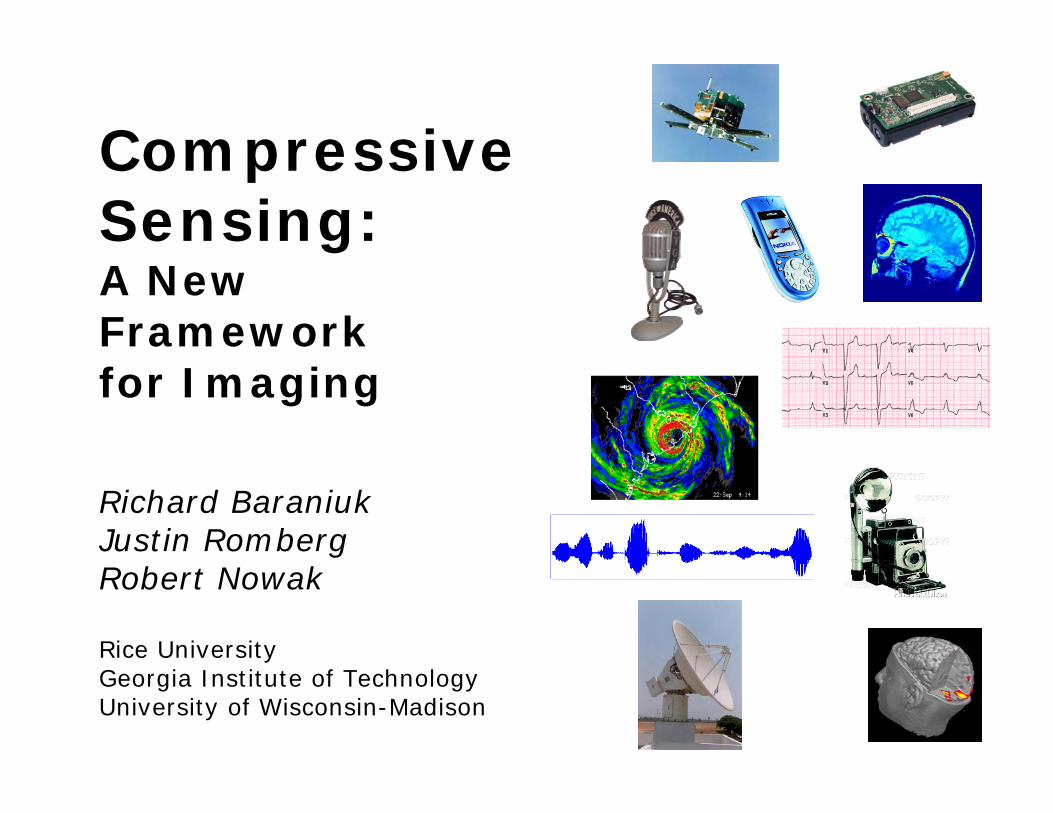
Richard BaraniukJustin RombergRobert Nowak
Rice UniversityGeorgia Institute of TechnologyUniversity of Wisconsin-Madison
CompressiveSensing:A NewFrameworkfor Imaging
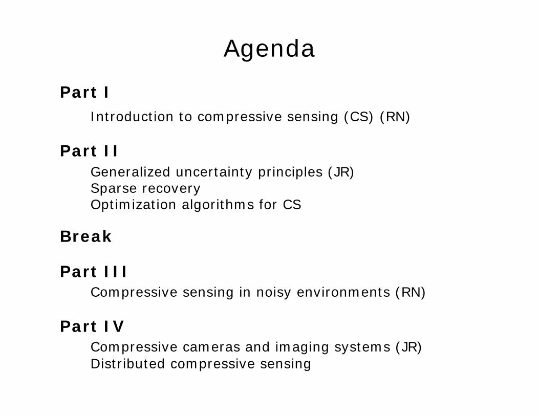
Agenda
Part IIntroduction to compressive sensing (CS) (RN)
Part IIGeneralized uncertainty principles (JR)Sparse recoveryOptimization algorithms for CS
Break
Part IIICompressive sensing in noisy environments (RN)
Part IVCompressive cameras and imaging systems (JR)Distributed compressive sensing
Part I –Introduction to
Compressive Sensing
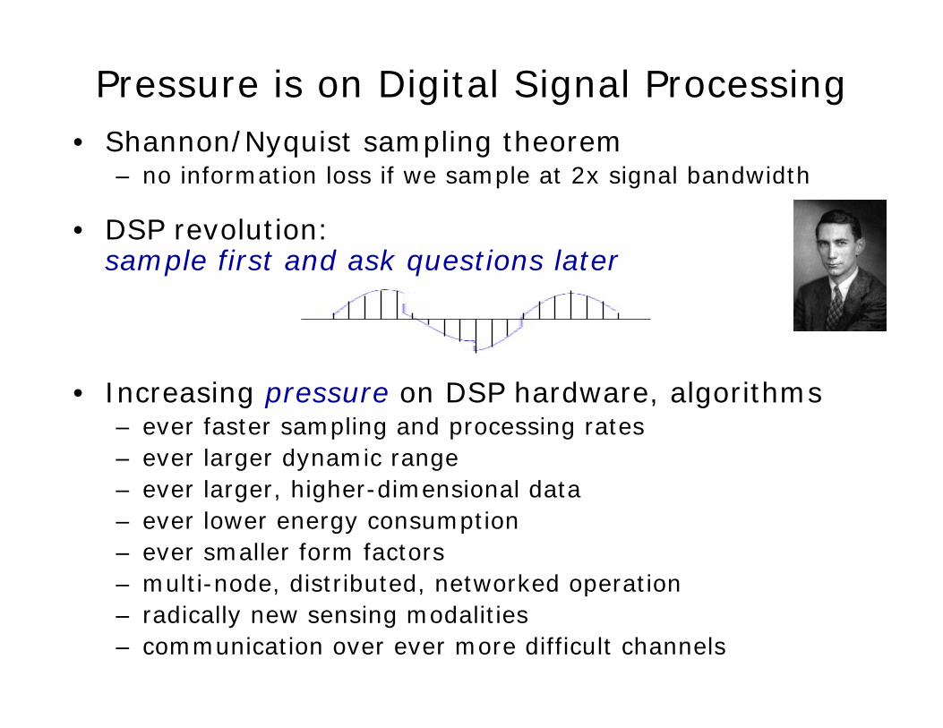
Pressure is on Digital Signal Processing• Shannon/Nyquist sampling theorem
– no information loss if we sample at 2x signal bandwidth
• DSP revolution: sample first and ask questions later
• Increasing pressure on DSP hardware, algorithms– ever faster sampling and processing rates– ever larger dynamic range– ever larger, higher-dimensional data– ever lower energy consumption– ever smaller form factors– multi-node, distributed, networked operation– radically new sensing modalities– communication over ever more difficult channels
Pressure is on Image Processing
• increasing pressure on signal/image processing hardware and algs to support
higher resolution / denser sampling» ADCs, cameras, imaging systems, …
+large numbers of signals, images, …
» multi-view target data bases, camera arrays and networks, pattern recognition systems,
+increasing numbers of modalities
» acoustic, seismic, RF, visual, IR, SAR, …
=deluge of datadeluge of data
» how to acquire, store, fuse, process efficiently?

Background:Structure of Natural Images
Images
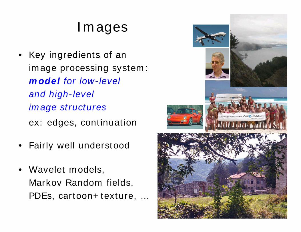
• Key ingredients of an image processing system:model for low-level and high-levelimage structures
ex: edges, continuation
• Fairly well understood
• Wavelet models,Markov Random fields, PDEs, cartoon+texture, …
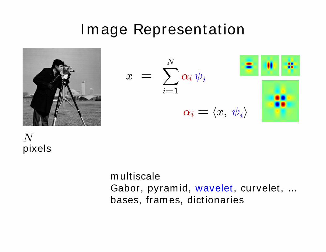
Image Representation
multiscaleGabor, pyramid, wavelet, curvelet, …bases, frames, dictionaries
pixels
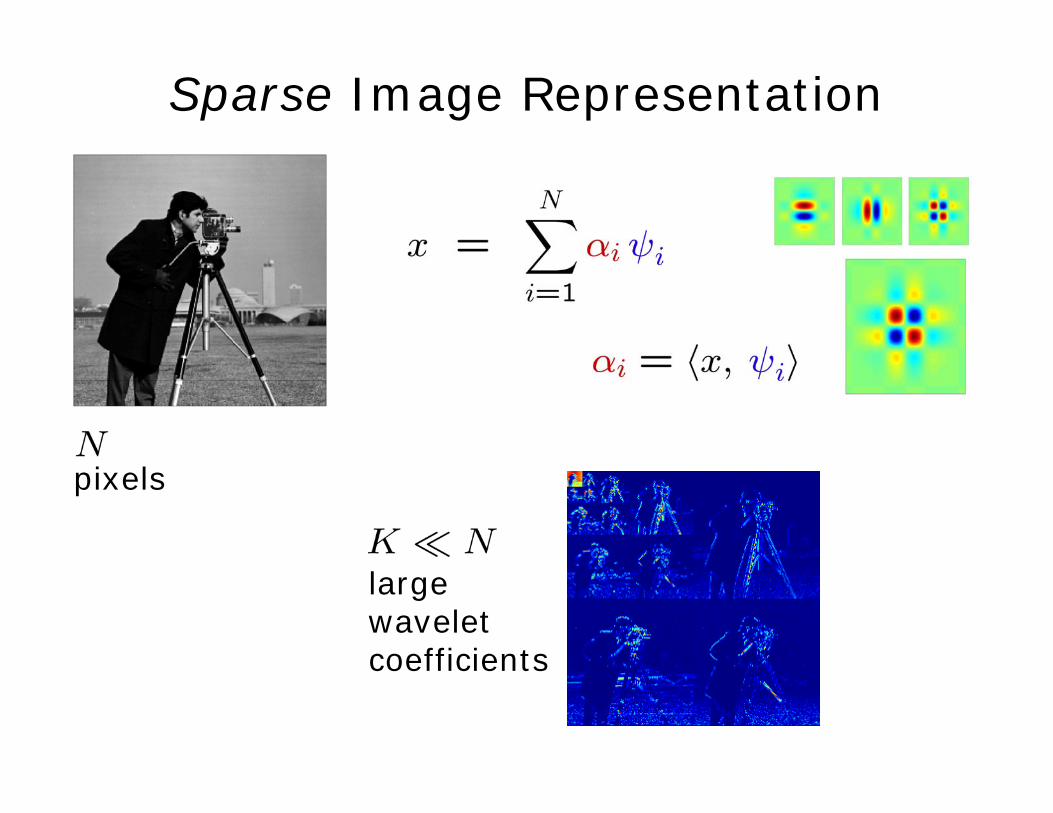
Sparse Image Representation
pixels
largewaveletcoefficients
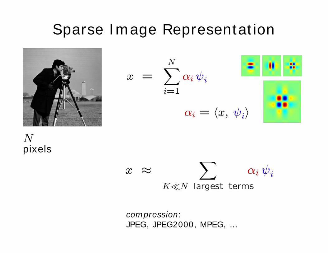
Sparse Image Representation
pixels
compression:JPEG, JPEG2000, MPEG, …
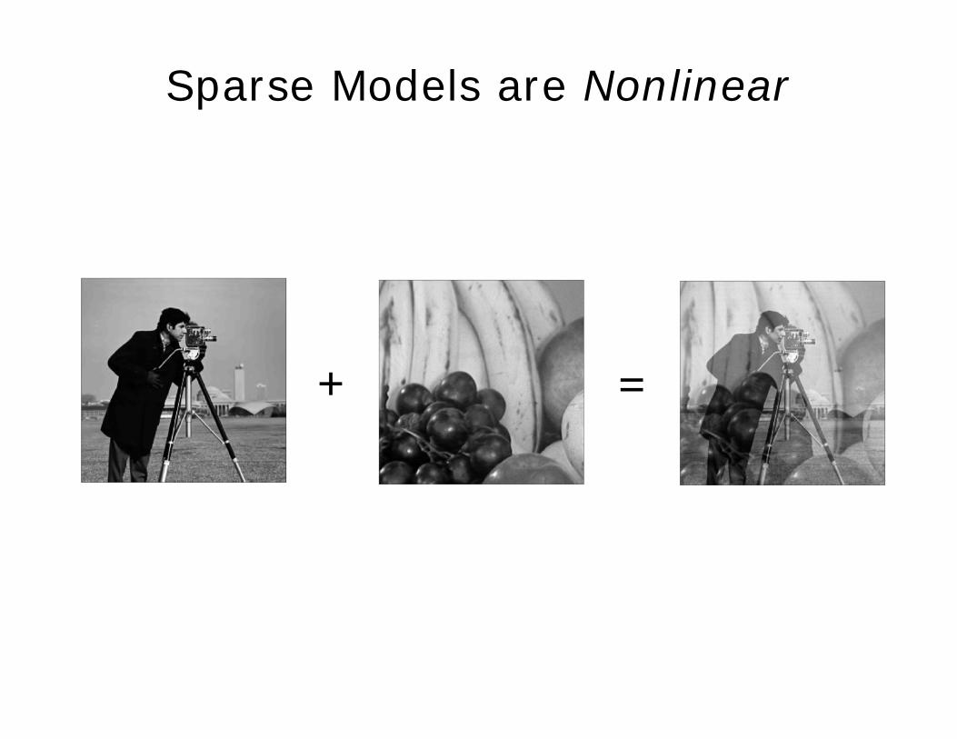
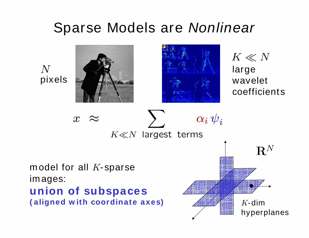
Sparse Models are Nonlinear
+ =

Sparse Models are Nonlinear
pixelslargewaveletcoefficients
model for all K-sparseimages
Sparse Models are Nonlinear
K-dimhyperplanes
pixelslargewaveletcoefficients
model for all K-sparseimages: union of subspaces(aligned with coordinate axes)
Overview of Compressive Imaging
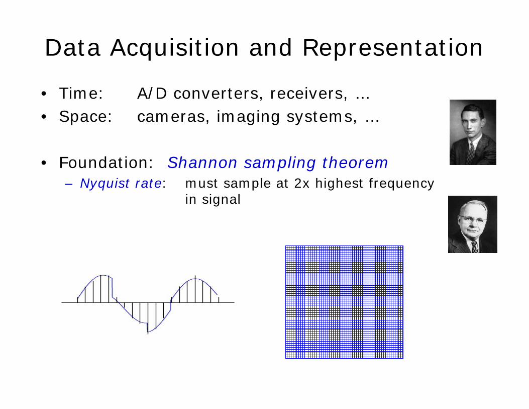
Data Acquisition and Representation
• Time: A/D converters, receivers, …• Space: cameras, imaging systems, …
• Foundation: Shannon sampling theorem– Nyquist rate: must sample at 2x highest frequency
in signal
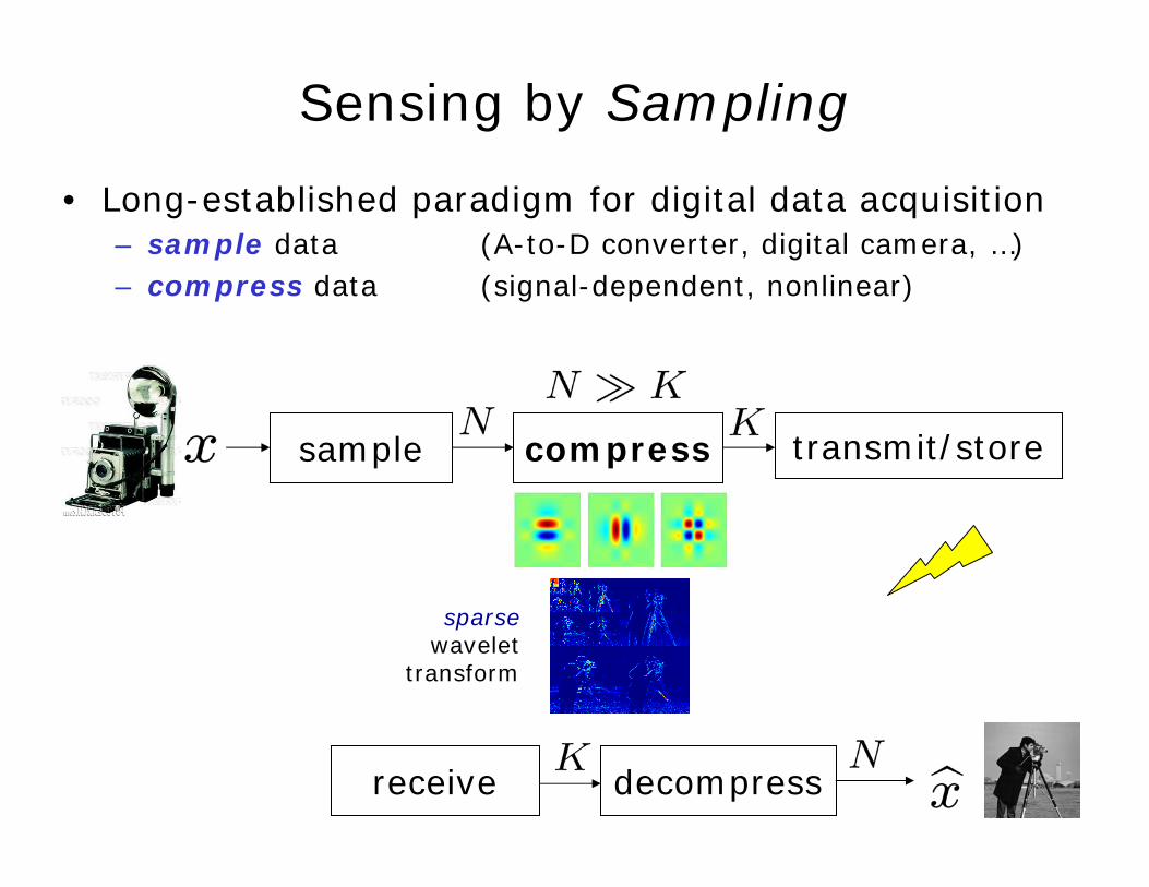
Sensing by Sampling
• Long-established paradigm for digital data acquisition– sample data (A-to-D converter, digital camera, …) – compress data (signal-dependent, nonlinear)
compress transmit/store
receive decompress
sample
sparsewavelet
transform
From Samples to Measurements
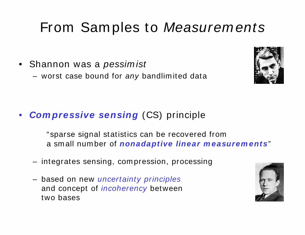
• Shannon was a pessimist– worst case bound for any bandlimited data
• Compressive sensing (CS) principle
“sparse signal statistics can be recovered from a small number of nonadaptive linear measurements”
– integrates sensing, compression, processing
– based on new uncertainty principlesand concept of incoherency between two bases
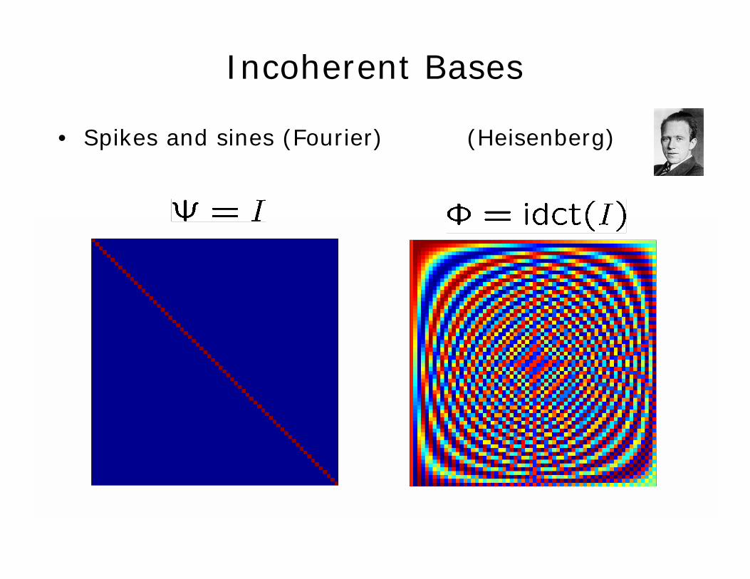
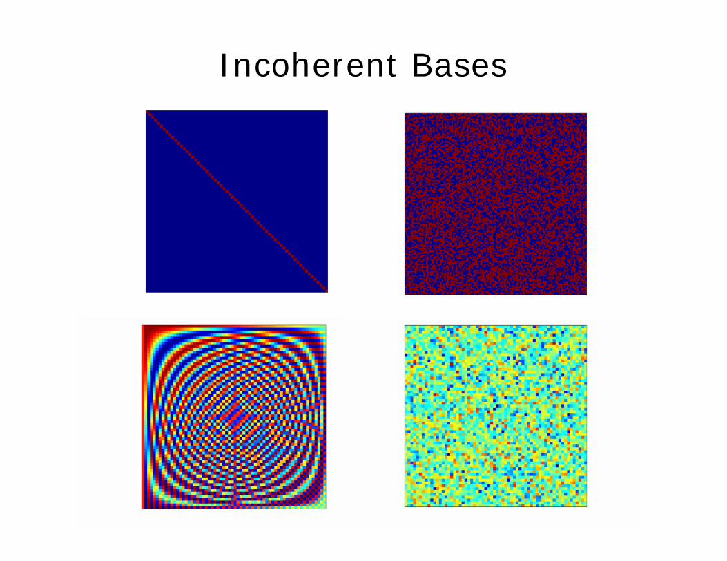
Incoherent Bases
• Spikes and sines (Fourier) (Heisenberg)
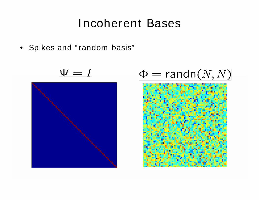
Incoherent Bases
• Spikes and “random basis”
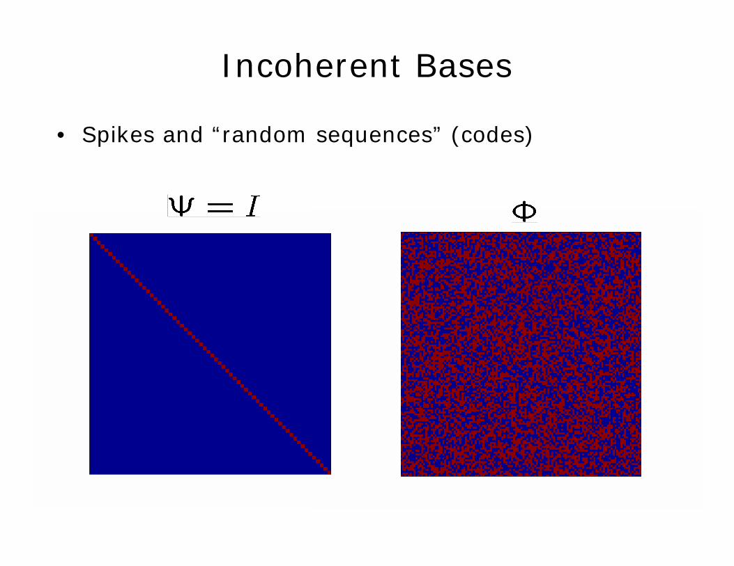
Incoherent Bases
• Spikes and “random sequences” (codes)
Incoherent Bases
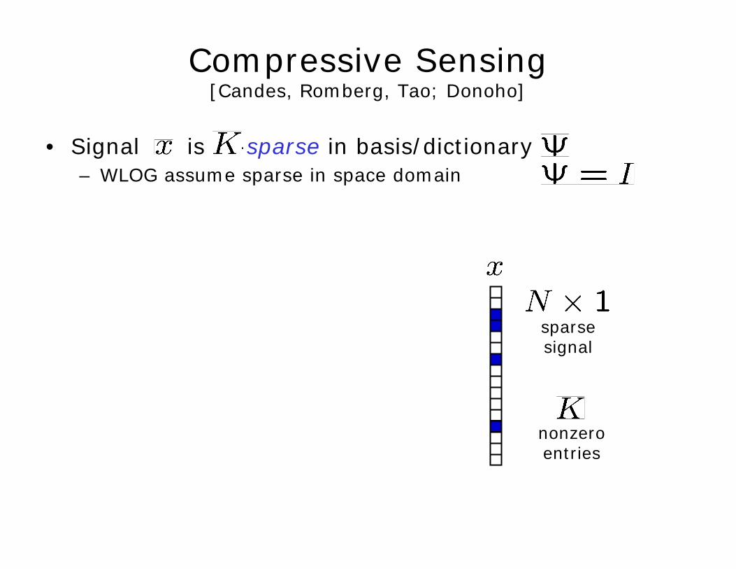
Compressive Sensing [Candes, Romberg, Tao; Donoho]
• Signal is -sparse in basis/dictionary– WLOG assume sparse in space domain
sparsesignal
nonzeroentries
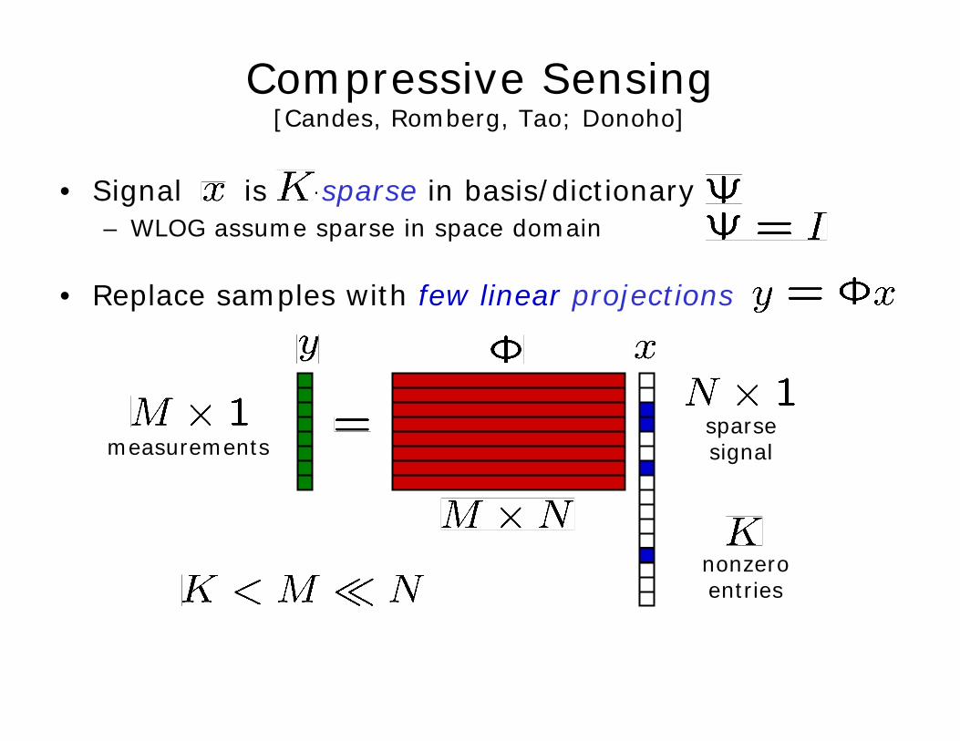
Compressive Sensing [Candes, Romberg, Tao; Donoho]
• Signal is -sparse in basis/dictionary– WLOG assume sparse in space domain
• Replace samples with few linear projections
measurementssparsesignal
nonzeroentries
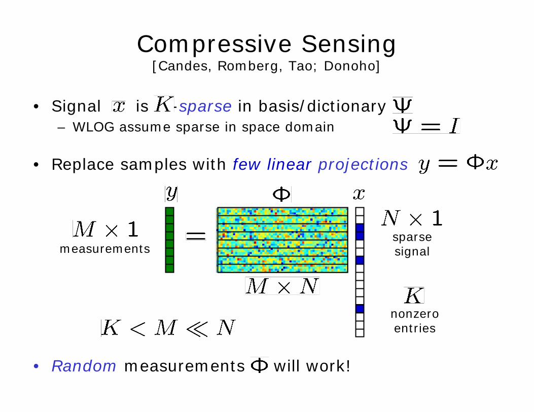
Compressive Sensing [Candes, Romberg, Tao; Donoho]
• Signal is -sparse in basis/dictionary– WLOG assume sparse in space domain
• Replace samples with few linear projections
• Random measurements will work!
measurementssparsesignal
nonzeroentries
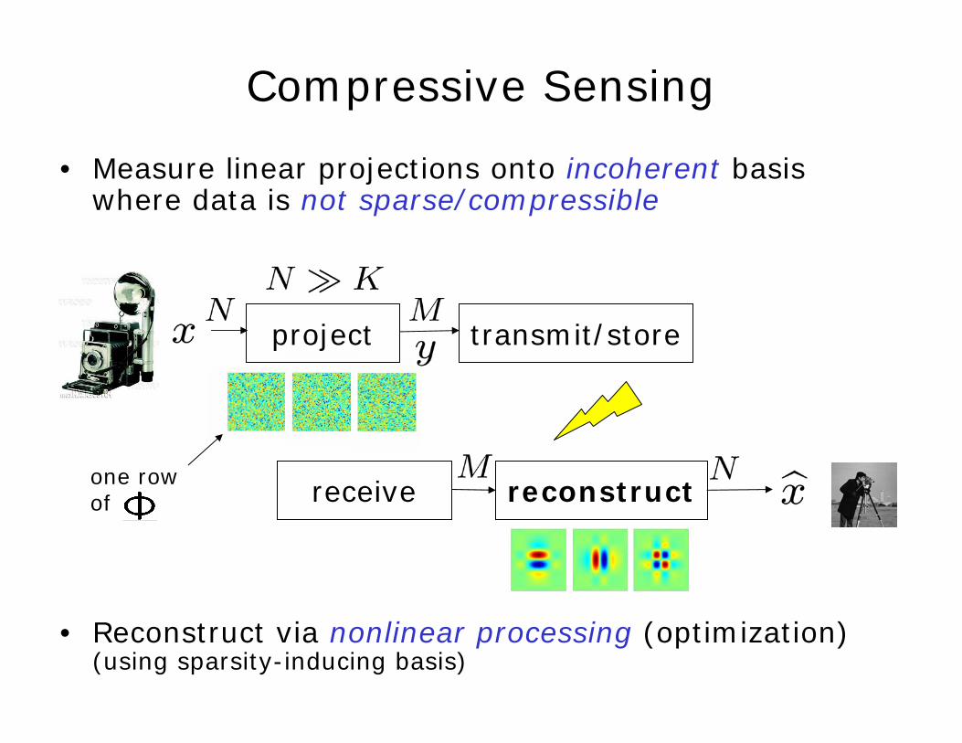
• Measure linear projections onto incoherent basis where data is not sparse/compressible
• Reconstruct via nonlinear processing (optimization)(using sparsity-inducing basis)
Compressive Sensing
project transmit/store
receive reconstructone row of
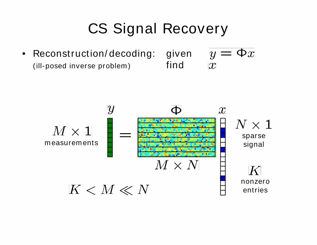
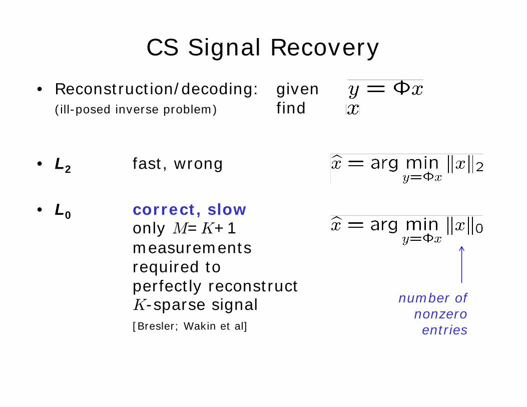
• Reconstruction/decoding: given(ill-posed inverse problem) find
CS Signal Recovery
measurementssparsesignal
nonzeroentries
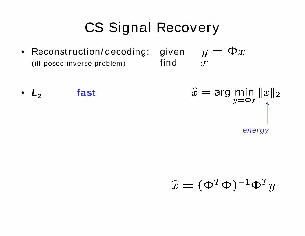
• Reconstruction/decoding: given(ill-posed inverse problem) find
• L2 fast
CS Signal Recovery
energy
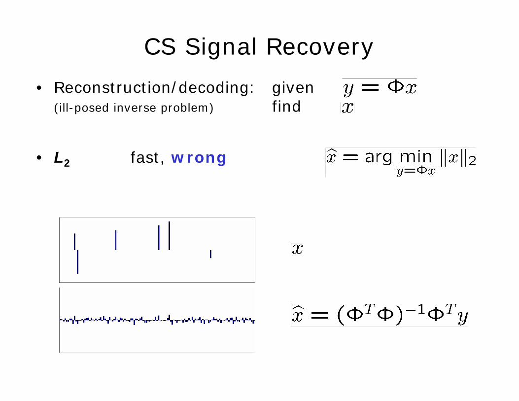
• Reconstruction/decoding: given(ill-posed inverse problem) find
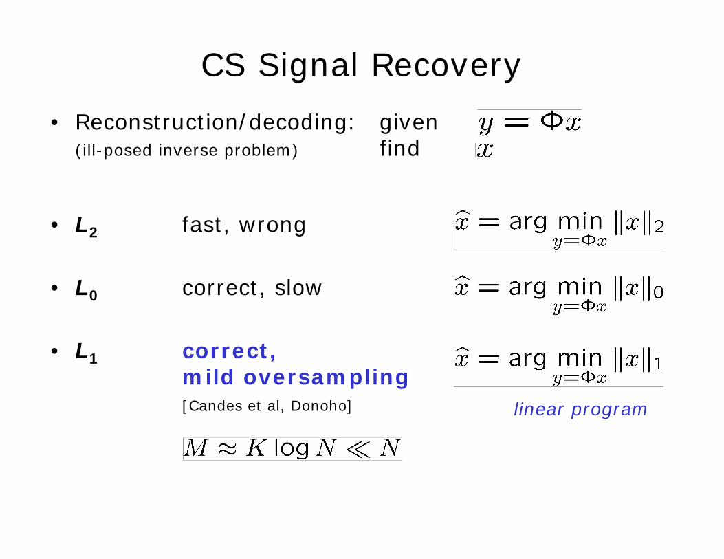
• L2 fast, wrong
CS Signal Recovery
• Reconstruction/decoding: given(ill-posed inverse problem) find
• L2 fast, wrong
• L0 correct, slowonly M=K+1 measurements required to perfectly reconstruct K-sparse signal[Bresler; Wakin et al]
CS Signal Recovery
number ofnonzeroentries
• Reconstruction/decoding: given(ill-posed inverse problem) find
• L2 fast, wrong
• L0 correct, slow
• L1 correct, mild oversampling[Candes et al, Donoho]
CS Signal Recovery
linear program
Part II –Generalized
Uncertainty Principles and
CS Recovery Algorithms
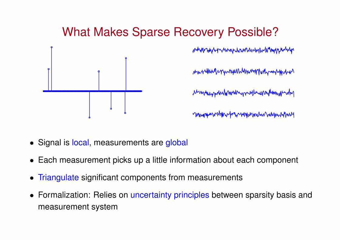
What Makes Sparse Recovery Possible?
• Signal is local, measurements are global
• Each measurement picks up a little information about each component
• Triangulate significant components from measurements
• Formalization: Relies on uncertainty principles between sparsity basis andmeasurement system

Uncertainty Principles
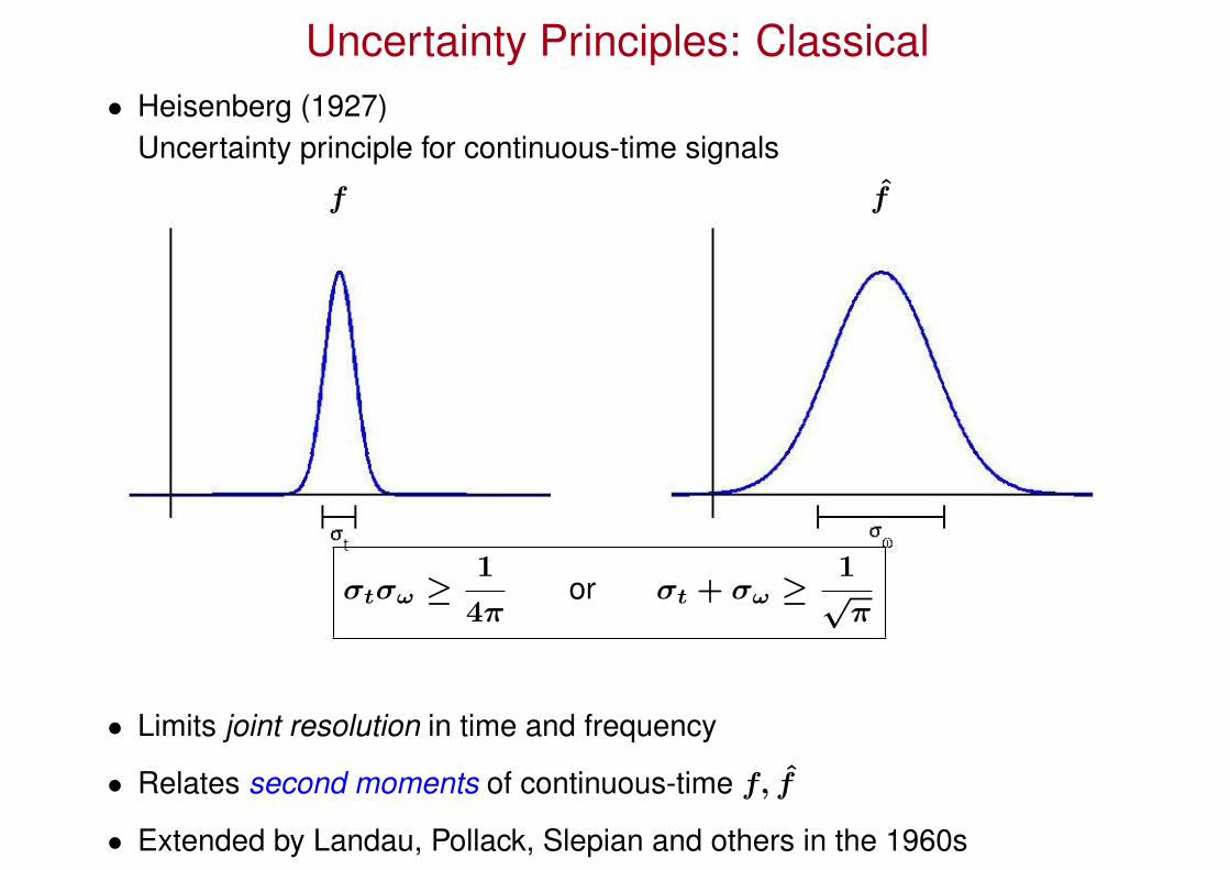
Uncertainty Principles: Classical• Heisenberg (1927)
Uncertainty principle for continuous-time signals
f f
σtσω ≥1
4πor σt + σω ≥
1√
π
• Limits joint resolution in time and frequency
• Relates second moments of continuous-time f, f
• Extended by Landau, Pollack, Slepian and others in the 1960s
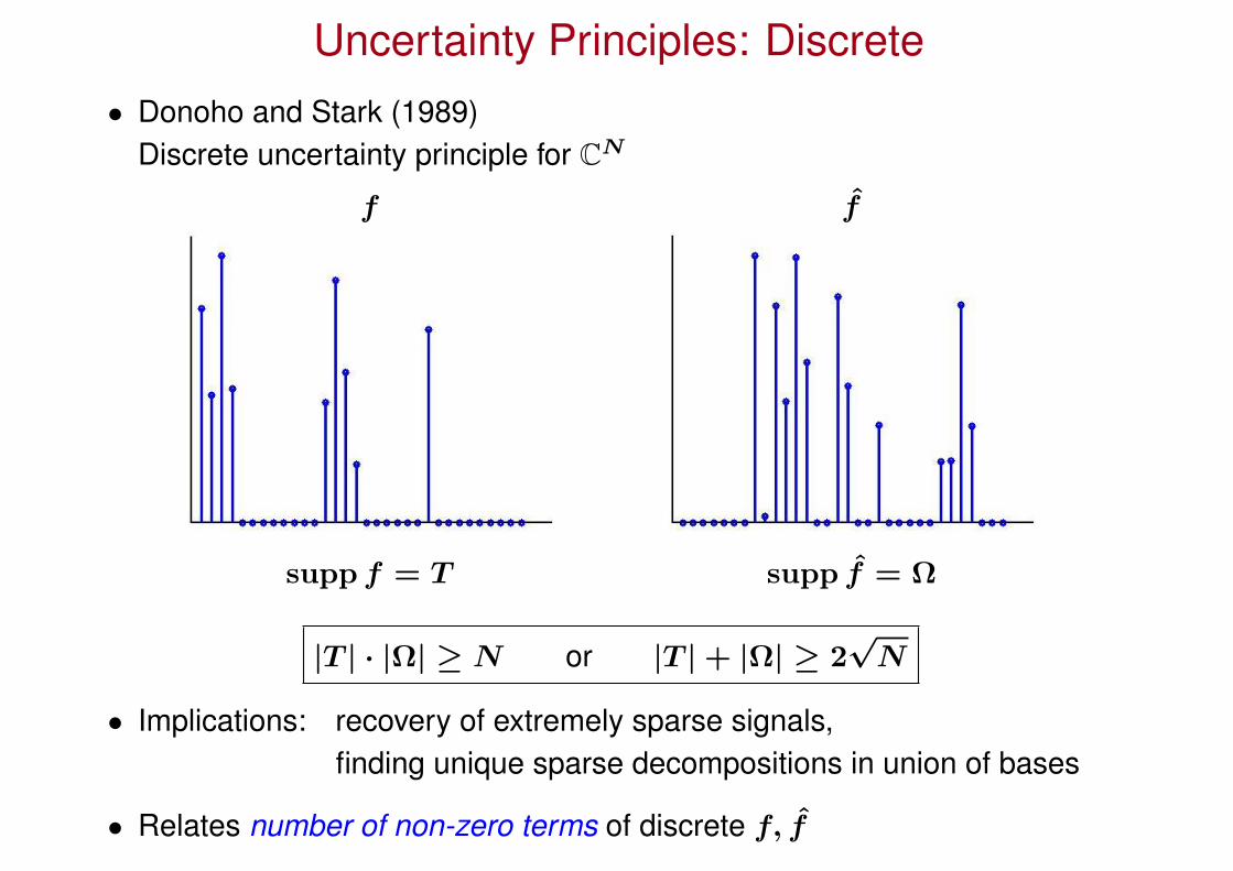
Uncertainty Principles: Discrete• Donoho and Stark (1989)
Discrete uncertainty principle for CN
f f
supp f = T supp f = Ω
|T | · |Ω| ≥ N or |T | + |Ω| ≥ 2√
N
• Implications: recovery of extremely sparse signals,finding unique sparse decompositions in union of bases
• Relates number of non-zero terms of discrete f, f
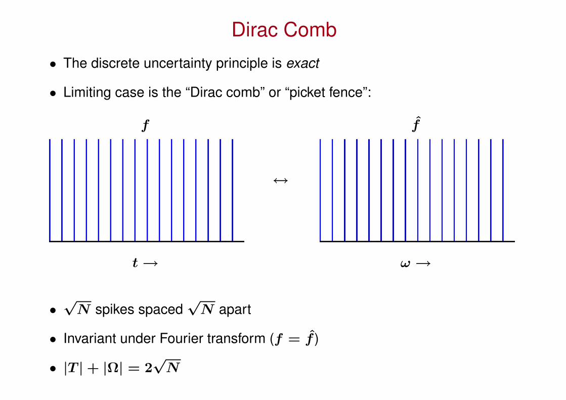
Dirac Comb
• The discrete uncertainty principle is exact
• Limiting case is the “Dirac comb” or “picket fence”:
f f
↔
t → ω →
•√
N spikes spaced√
N apart
• Invariant under Fourier transform (f = f )
• |T | + |Ω| = 2√
N
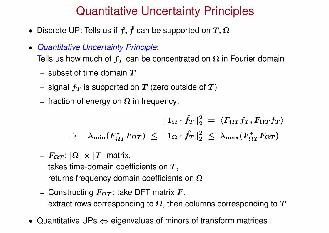
Quantitative Uncertainty Principles
• Discrete UP: Tells us if f, f can be supported on T, Ω
• Quantitative Uncertainty Principle:Tells us how much of fT can be concentrated on Ω in Fourier domain
– subset of time domain T
– signal fT is supported on T (zero outside of T )
– fraction of energy on Ω in frequency:
‖1Ω · fT ‖22 = 〈FΩT fT , FΩT fT 〉
⇒ λmin(F ∗ΩT FΩT ) ≤ ‖1Ω · fT ‖2
2 ≤ λmax(F ∗ΩT FΩT )
– FΩT : |Ω| × |T | matrix,takes time-domain coefficients on T ,returns frequency domain coefficients on Ω
– Constructing FΩT : take DFT matrix F ,extract rows corresponding to Ω, then columns corresponding to T
• Quantitative UPs ⇔ eigenvalues of minors of transform matrices
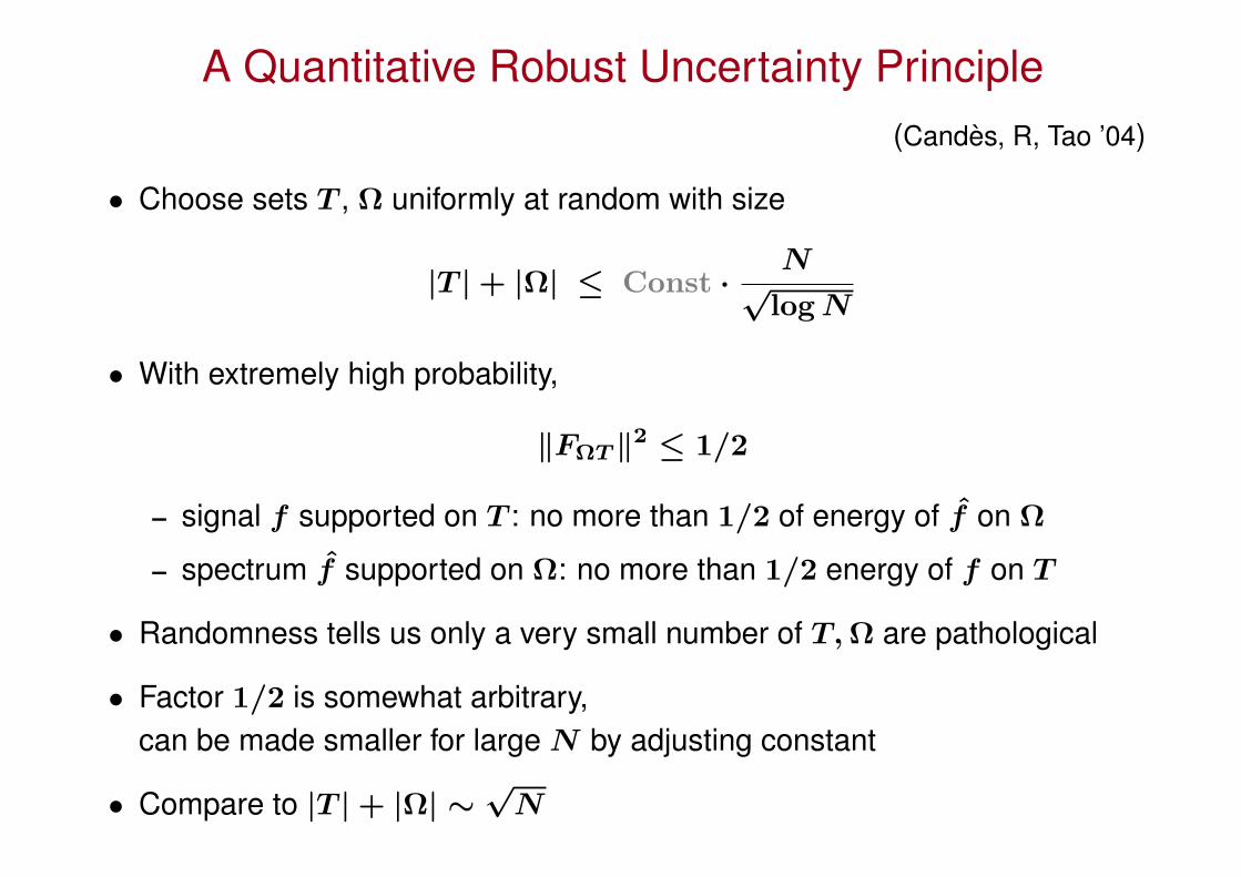
A Quantitative Robust Uncertainty Principle(Candes, R, Tao ’04)
• Choose sets T , Ω uniformly at random with size
|T | + |Ω| ≤ Const ·N
√log N
• With extremely high probability,
‖FΩT ‖2 ≤ 1/2
– signal f supported on T : no more than 1/2 of energy of f on Ω
– spectrum f supported on Ω: no more than 1/2 energy of f on T
• Randomness tells us only a very small number of T, Ω are pathological
• Factor 1/2 is somewhat arbitrary,can be made smaller for large N by adjusting constant
• Compare to |T | + |Ω| ∼√
N
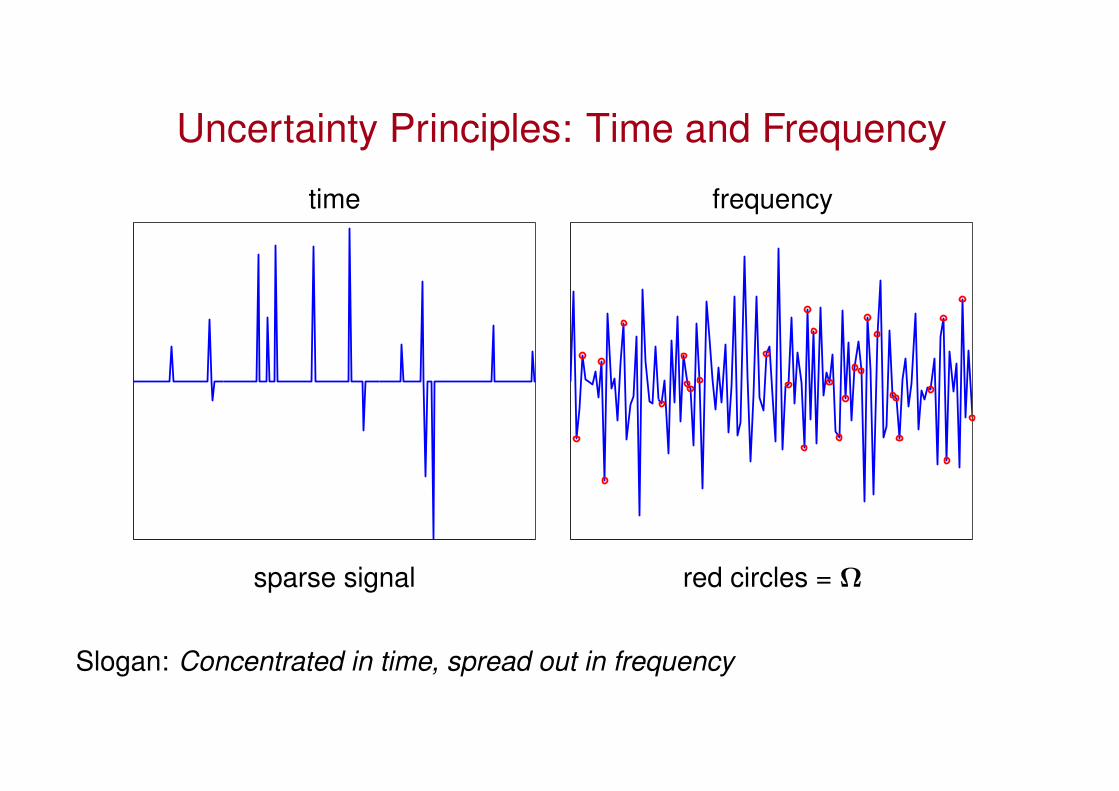
Uncertainty Principles: Time and Frequency
time frequency
sparse signal red circles = Ω
Slogan: Concentrated in time, spread out in frequency
Recovering a Spectrally Sparse Signal froma Small Number of Samples
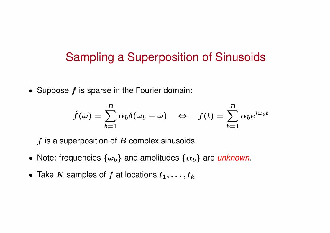
Sampling a Superposition of Sinusoids
• Suppose f is sparse in the Fourier domain:
f(ω) =B∑
b=1
αbδ(ωb − ω) ⇔ f(t) =B∑
b=1
αbeiωbt
f is a superposition of B complex sinusoids.
• Note: frequencies ωb and amplitudes αb are unknown.
• Take K samples of f at locations t1, . . . , tk
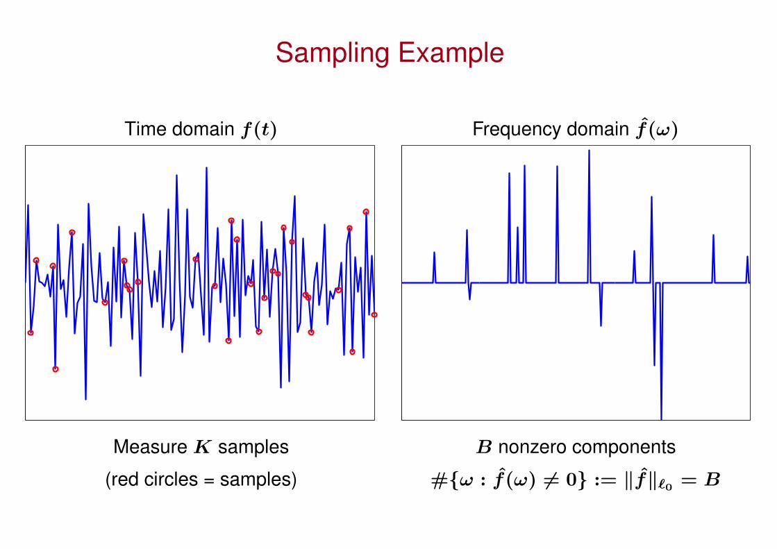
Sampling Example
Time domain f(t) Frequency domain f(ω)
Measure K samples B nonzero components
(red circles = samples) #ω : f(ω) 6= 0 := ‖f‖`0 = B
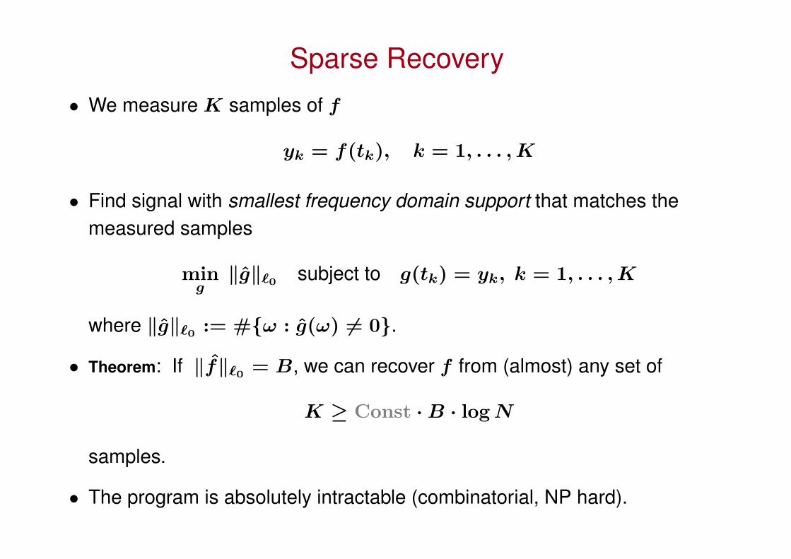
Sparse Recovery
• We measure K samples of f
yk = f(tk), k = 1, . . . , K
• Find signal with smallest frequency domain support that matches themeasured samples
ming
‖g‖`0 subject to g(tk) = yk, k = 1, . . . , K
where ‖g‖`0 := #ω : g(ω) 6= 0.
• Theorem: If ‖f‖`0 = B, we can recover f from (almost) any set of
K ≥ Const · B · log N
samples.
• The program is absolutely intractable (combinatorial, NP hard).
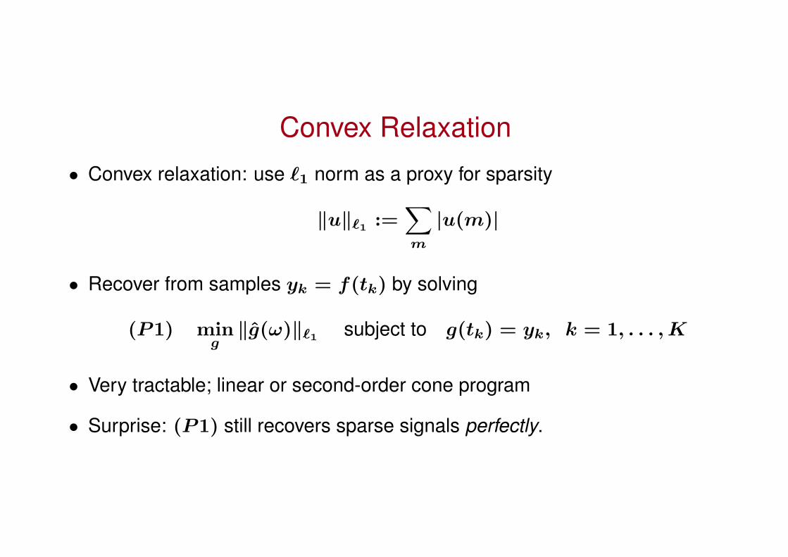
Convex Relaxation
• Convex relaxation: use `1 norm as a proxy for sparsity
‖u‖`1 :=∑m
|u(m)|
• Recover from samples yk = f(tk) by solving
(P1) ming
‖g(ω)‖`1 subject to g(tk) = yk, k = 1, . . . , K
• Very tractable; linear or second-order cone program
• Surprise: (P1) still recovers sparse signals perfectly.
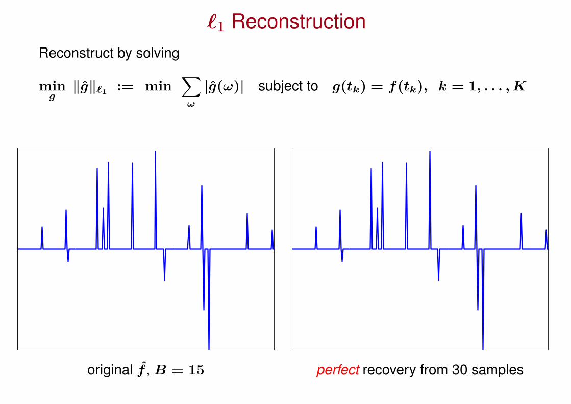
`1 ReconstructionReconstruct by solving
ming
‖g‖`1 := min∑ω
|g(ω)| subject to g(tk) = f(tk), k = 1, . . . , K
original f , B = 15 perfect recovery from 30 samples
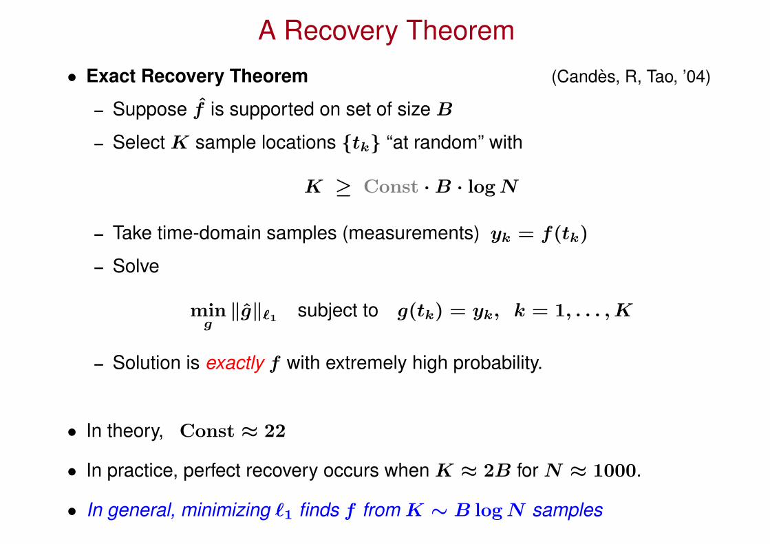
A Recovery Theorem
• Exact Recovery Theorem (Candes, R, Tao, ’04)
– Suppose f is supported on set of size B
– Select K sample locations tk “at random” with
K ≥ Const · B · log N
– Take time-domain samples (measurements) yk = f(tk)
– Solve
ming
‖g‖`1 subject to g(tk) = yk, k = 1, . . . , K
– Solution is exactly f with extremely high probability.
• In theory, Const ≈ 22
• In practice, perfect recovery occurs when K ≈ 2B for N ≈ 1000.
• In general, minimizing `1 finds f from K ∼ B log N samples
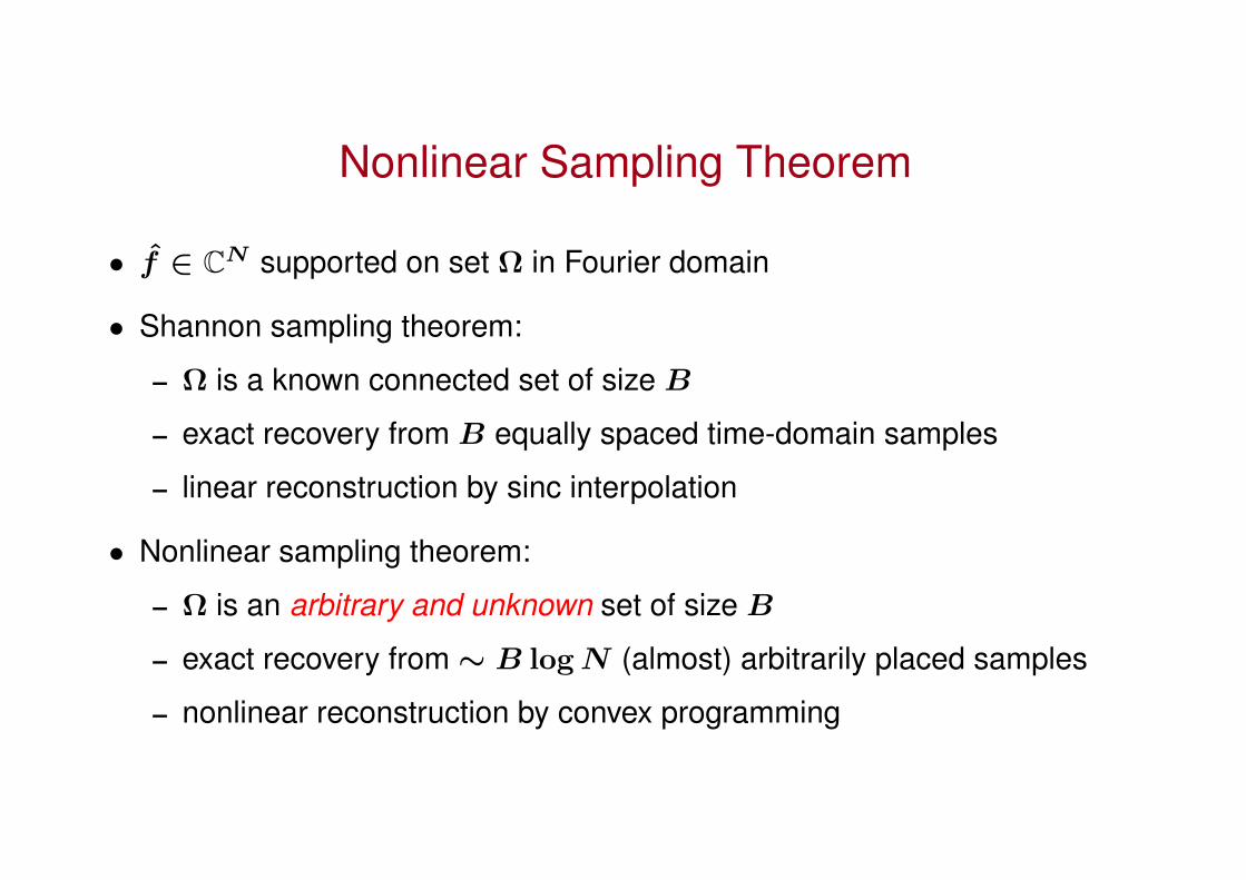
Nonlinear Sampling Theorem
• f ∈ CN supported on set Ω in Fourier domain
• Shannon sampling theorem:
– Ω is a known connected set of size B
– exact recovery from B equally spaced time-domain samples
– linear reconstruction by sinc interpolation
• Nonlinear sampling theorem:
– Ω is an arbitrary and unknown set of size B
– exact recovery from ∼ B log N (almost) arbitrarily placed samples
– nonlinear reconstruction by convex programming
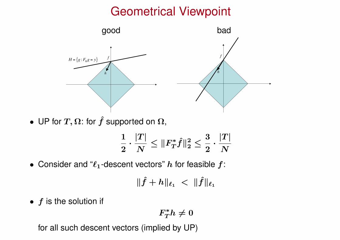
Geometrical Viewpointgood bad
!
H = g :F"g = y
!
f
!
h !
f
!
h
• UP for T, Ω: for f supported on Ω,
1
2·
|T |N
≤ ‖F ∗T f‖2
2 ≤3
2·
|T |N
• Consider and “`1-descent vectors” h for feasible f :
‖f + h‖`1 < ‖f‖`1
• f is the solution ifF ∗
T h 6= 0
for all such descent vectors (implied by UP)

Extensions
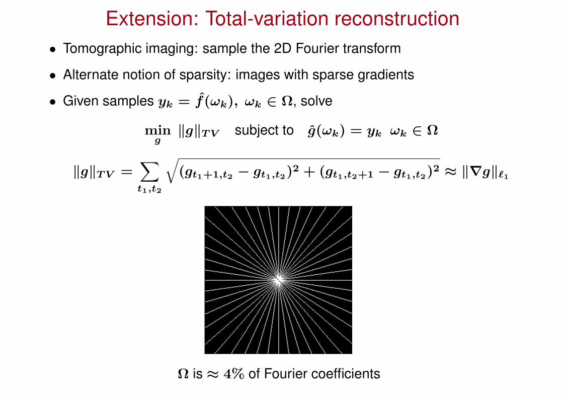
Extension: Total-variation reconstruction• Tomographic imaging: sample the 2D Fourier transform
• Alternate notion of sparsity: images with sparse gradients
• Given samples yk = f(ωk), ωk ∈ Ω, solve
ming
‖g‖T V subject to g(ωk) = yk ωk ∈ Ω
‖g‖T V =∑t1,t2
√(gt1+1,t2 − gt1,t2)2 + (gt1,t2+1 − gt1,t2)2 ≈ ‖∇g‖`1
Ω is ≈ 4% of Fourier coefficients
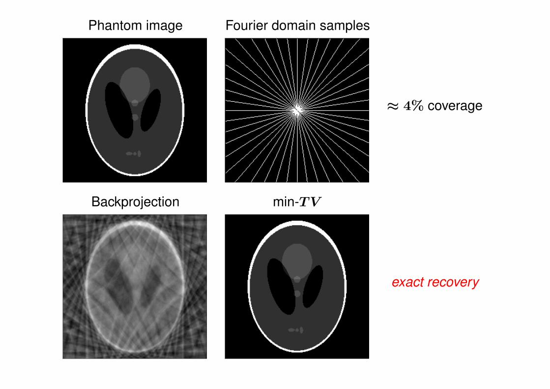
Phantom image Fourier domain samples
≈ 4% coverage
Backprojection min-TV
exact recovery
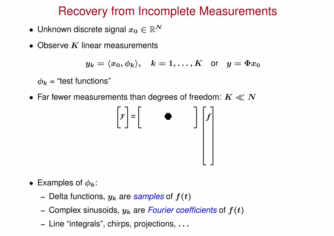
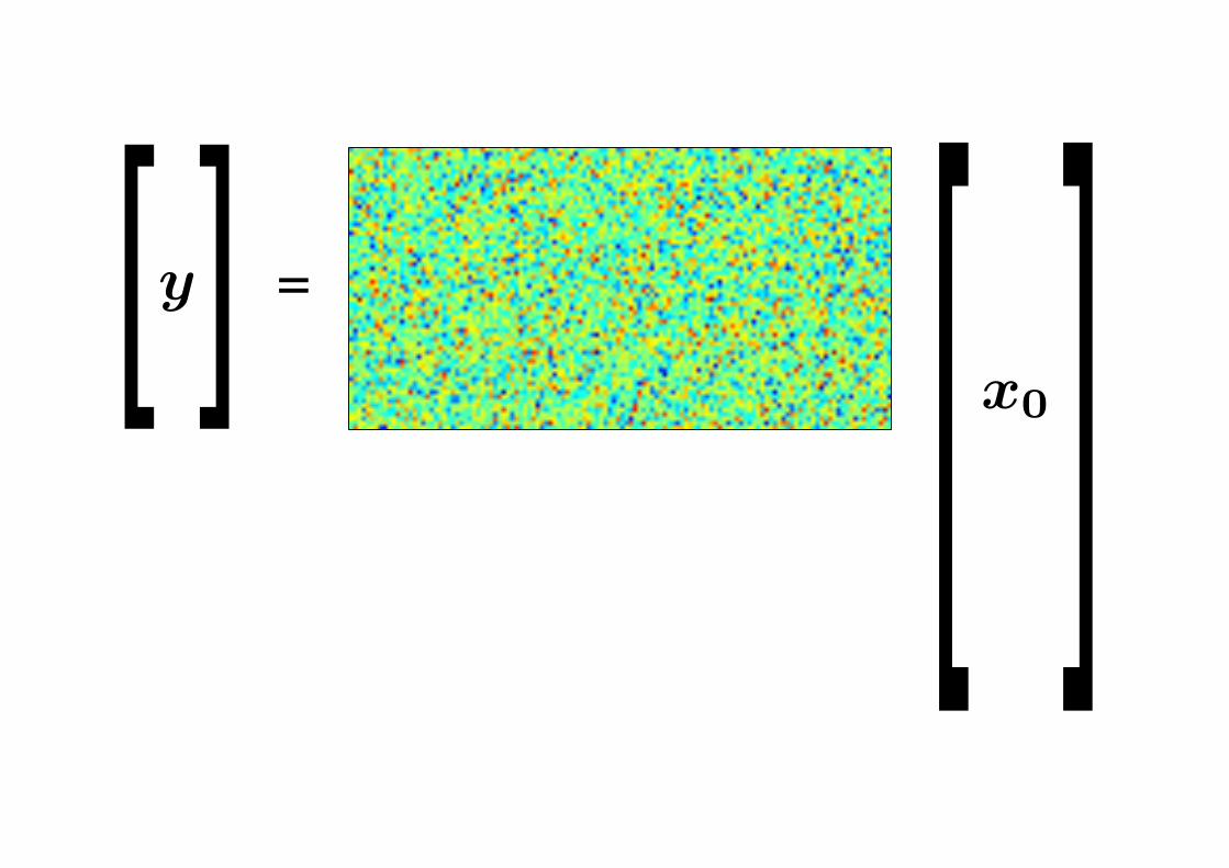
Recovery from Incomplete Measurements• Unknown discrete signal x0 ∈ RN
• Observe K linear measurements
yk = 〈x0, φk〉, k = 1, . . . , K or y = Φx0
φk = “test functions”
• Far fewer measurements than degrees of freedom: K N
y ! f=
• Examples of φk:
– Delta functions, yk are samples of f(t)
– Complex sinusoids, yk are Fourier coefficients of f(t)
– Line “integrals”, chirps, projections, . . .
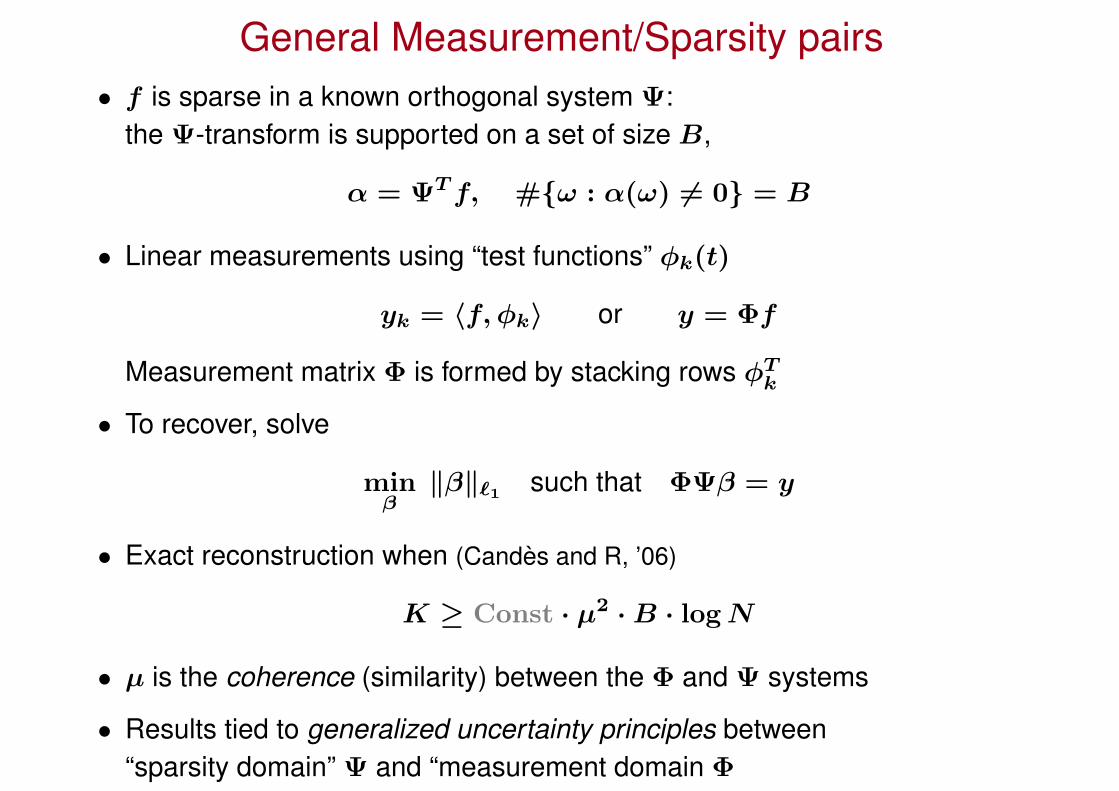
General Measurement/Sparsity pairs• f is sparse in a known orthogonal system Ψ:
the Ψ-transform is supported on a set of size B,
α = ΨT f, #ω : α(ω) 6= 0 = B
• Linear measurements using “test functions” φk(t)
yk = 〈f, φk〉 or y = Φf
Measurement matrix Φ is formed by stacking rows φTk
• To recover, solve
minβ
‖β‖`1 such that ΦΨβ = y
• Exact reconstruction when (Candes and R, ’06)
K ≥ Const · µ2 · B · log N
• µ is the coherence (similarity) between the Φ and Ψ systems
• Results tied to generalized uncertainty principles between“sparsity domain” Ψ and “measurement domain Φ
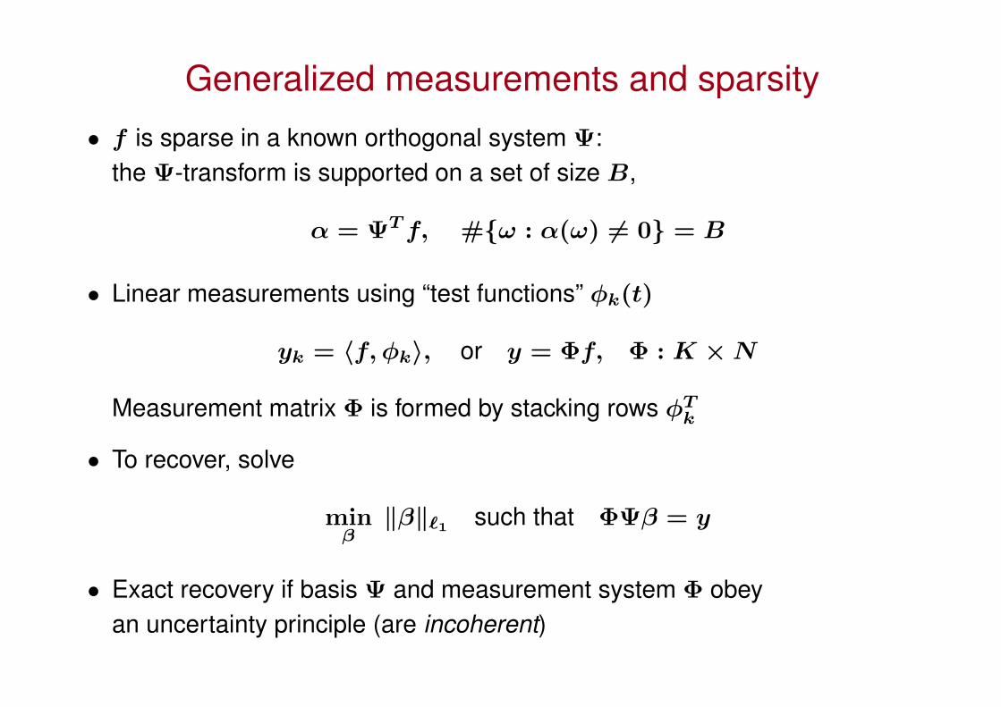
Generalized measurements and sparsity
• f is sparse in a known orthogonal system Ψ:the Ψ-transform is supported on a set of size B,
α = ΨT f, #ω : α(ω) 6= 0 = B
• Linear measurements using “test functions” φk(t)
yk = 〈f, φk〉, or y = Φf, Φ : K × N
Measurement matrix Φ is formed by stacking rows φTk
• To recover, solve
minβ
‖β‖`1 such that ΦΨβ = y
• Exact recovery if basis Ψ and measurement system Φ obeyan uncertainty principle (are incoherent)
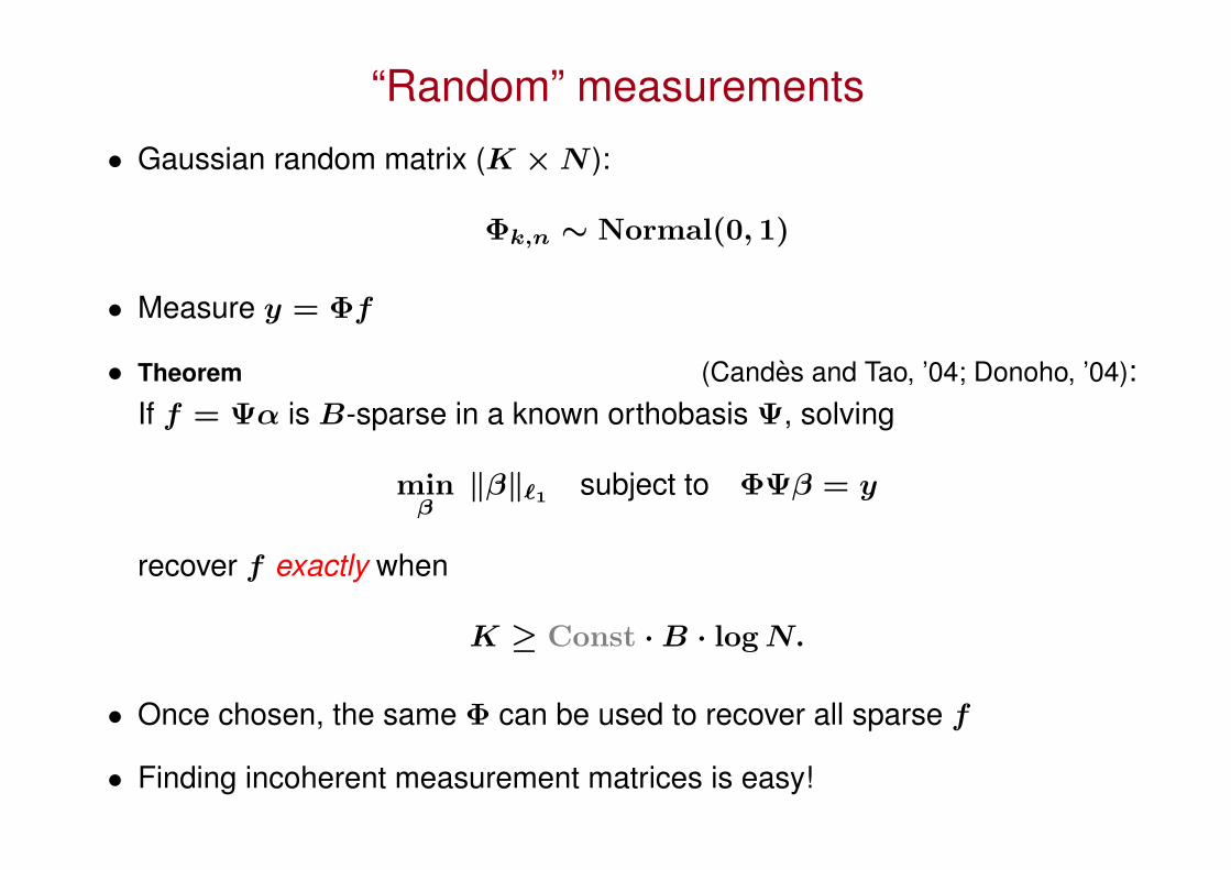
“Random” measurements
• Gaussian random matrix (K × N ):
Φk,n ∼ Normal(0, 1)
• Measure y = Φf
• Theorem (Candes and Tao, ’04; Donoho, ’04):If f = Ψα is B-sparse in a known orthobasis Ψ, solving
minβ
‖β‖`1 subject to ΦΨβ = y
recover f exactly when
K ≥ Const · B · log N.
• Once chosen, the same Φ can be used to recover all sparse f
• Finding incoherent measurement matrices is easy!
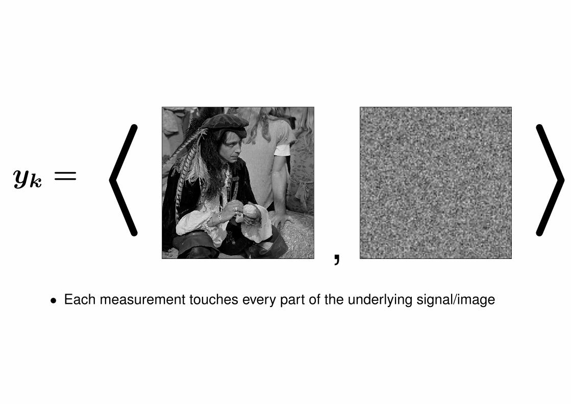
yk = 〈,
〉• Each measurement touches every part of the underlying signal/image
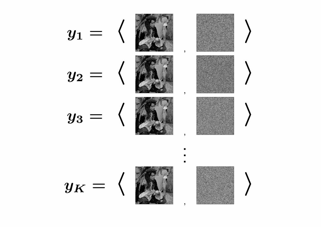
y1 = 〈,
〉
y2 = 〈,
〉
y3 = 〈,
〉...
yK = 〈,
〉
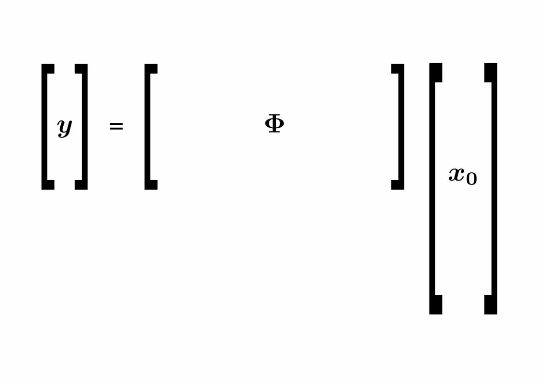
[y] = [ Φ ] [x0]
[y] = [x0]
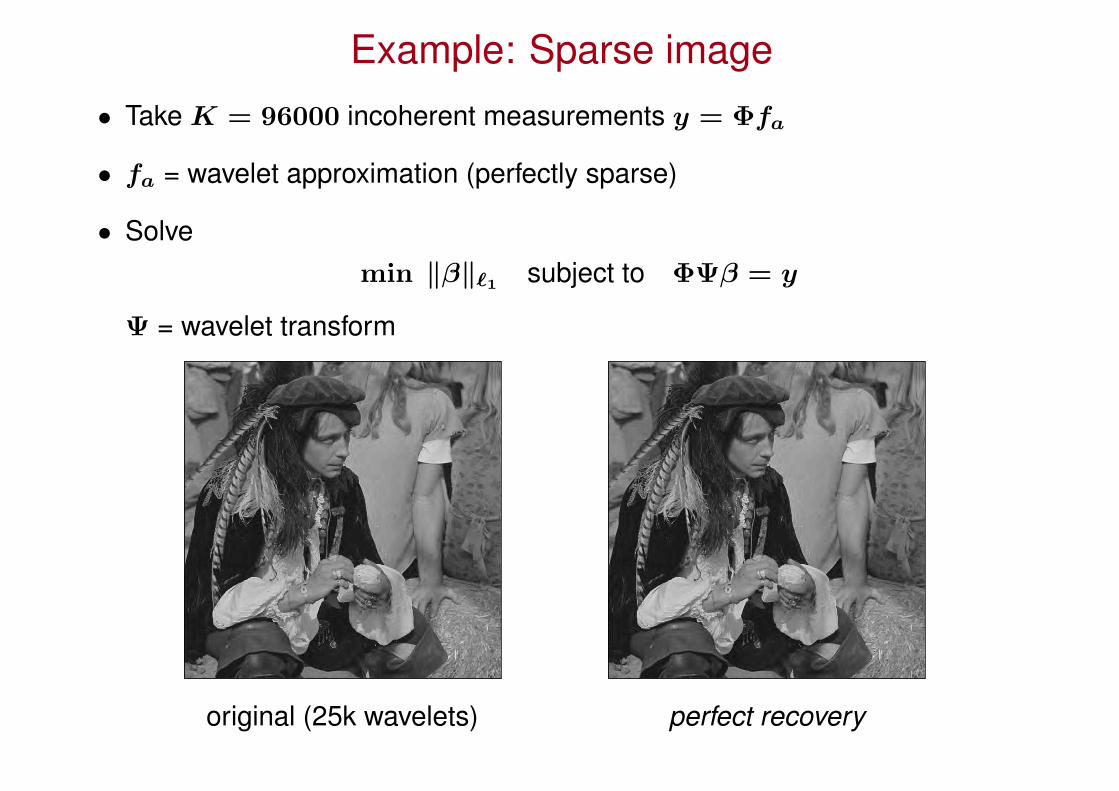
Example: Sparse image
• Take K = 96000 incoherent measurements y = Φfa
• fa = wavelet approximation (perfectly sparse)
• Solvemin ‖β‖`1 subject to ΦΨβ = y
Ψ = wavelet transform
original (25k wavelets) perfect recovery

Stability
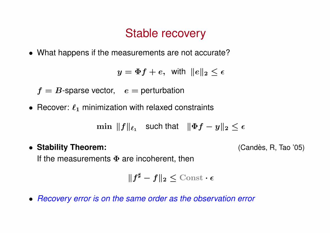
Stable recovery
• What happens if the measurements are not accurate?
y = Φf + e, with ‖e‖2 ≤ ε
f = B-sparse vector, e = perturbation
• Recover: `1 minimization with relaxed constraints
min ‖f‖`1 such that ‖Φf − y‖2 ≤ ε
• Stability Theorem: (Candes, R, Tao ’05)
If the measurements Φ are incoherent, then
‖f ] − f‖2 ≤ Const · ε
• Recovery error is on the same order as the observation error
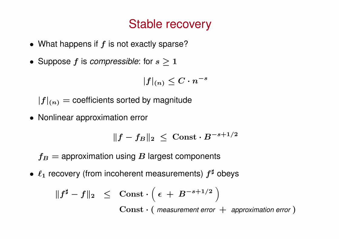
Stable recovery
• What happens if f is not exactly sparse?
• Suppose f is compressible: for s ≥ 1
|f |(n) ≤ C · n−s
|f |(n) = coefficients sorted by magnitude
• Nonlinear approximation error
‖f − fB‖2 ≤ Const · B−s+1/2
fB = approximation using B largest components
• `1 recovery (from incoherent measurements) f ] obeys
‖f ] − f‖2 ≤ Const ·(
ε + B−s+1/2)
Const · ( measurement error + approximation error )

Recovery via Convex Optimization
`1 minimization
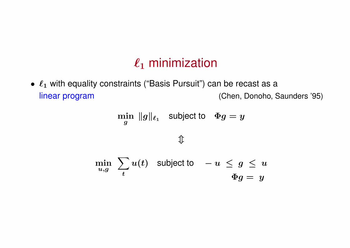
• `1 with equality constraints (“Basis Pursuit”) can be recast as alinear program (Chen, Donoho, Saunders ’95)
ming
‖g‖`1 subject to Φg = y
m
minu,g
∑t
u(t) subject to − u ≤ g ≤ u
Φg = y
Total-Variation Minimization
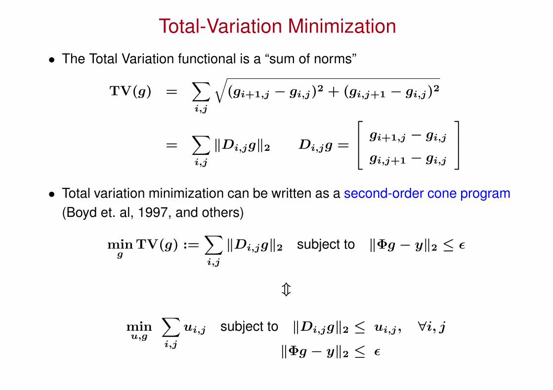
• The Total Variation functional is a “sum of norms”
TV(g) =∑i,j
√(gi+1,j − gi,j)2 + (gi,j+1 − gi,j)2
=∑i,j
‖Di,jg‖2 Di,jg =
gi+1,j − gi,j
gi,j+1 − gi,j
• Total variation minimization can be written as a second-order cone program
(Boyd et. al, 1997, and others)
ming
TV(g) :=∑i,j
‖Di,jg‖2 subject to ‖Φg − y‖2 ≤ ε
m
minu,g
∑i,j
ui,j subject to ‖Di,jg‖2 ≤ ui,j, ∀i, j
‖Φg − y‖2 ≤ ε
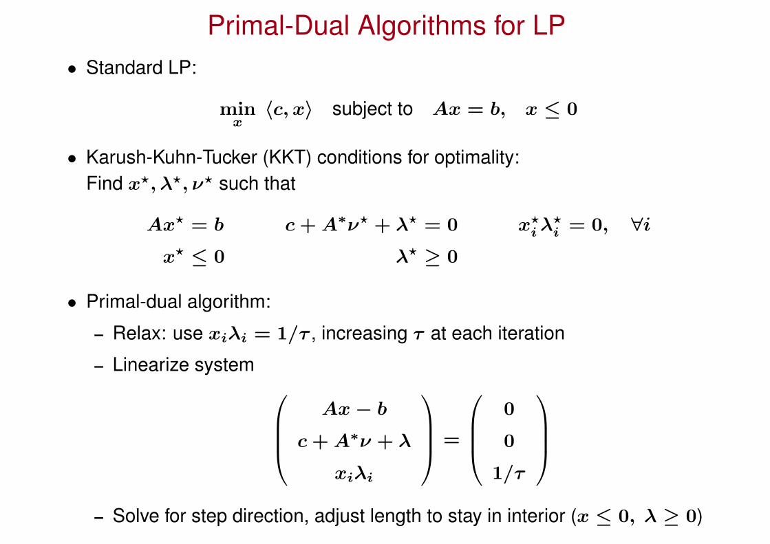
Primal-Dual Algorithms for LP• Standard LP:
minx
〈c, x〉 subject to Ax = b, x ≤ 0
• Karush-Kuhn-Tucker (KKT) conditions for optimality:Find x?, λ?, ν? such that
Ax? = b c + A∗ν? + λ? = 0 x?i λ?
i = 0, ∀i
x? ≤ 0 λ? ≥ 0
• Primal-dual algorithm:
– Relax: use xiλi = 1/τ , increasing τ at each iteration
– Linearize system Ax − b
c + A∗ν + λ
xiλi
=
0
0
1/τ
– Solve for step direction, adjust length to stay in interior (x ≤ 0, λ ≥ 0)
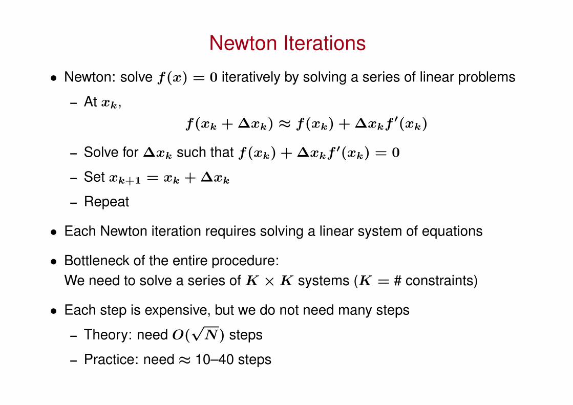
Newton Iterations
• Newton: solve f(x) = 0 iteratively by solving a series of linear problems
– At xk,f(xk + ∆xk) ≈ f(xk) + ∆xkf ′(xk)
– Solve for ∆xk such that f(xk) + ∆xkf ′(xk) = 0
– Set xk+1 = xk + ∆xk
– Repeat
• Each Newton iteration requires solving a linear system of equations
• Bottleneck of the entire procedure:We need to solve a series of K × K systems (K = # constraints)
• Each step is expensive, but we do not need many steps
– Theory: need O(√
N) steps
– Practice: need ≈ 10–40 steps
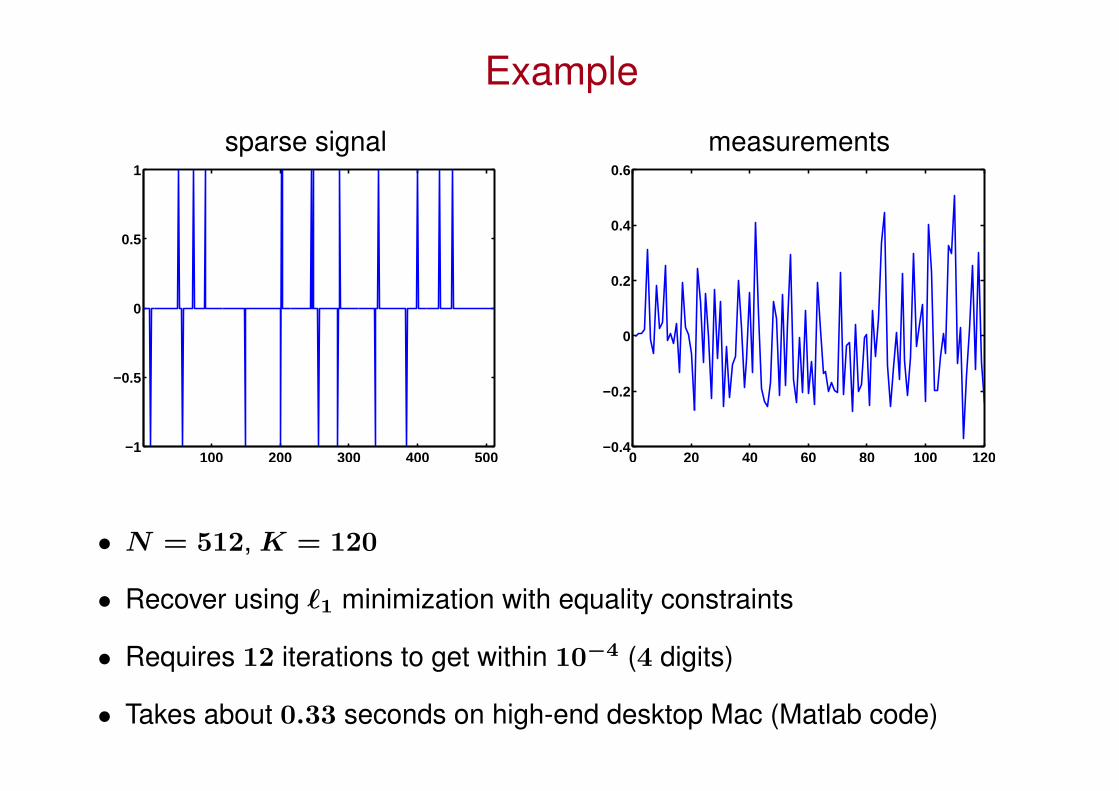
Example
sparse signal measurements
100 200 300 400 500−1
−0.5
0
0.5
1
0 20 40 60 80 100 120−0.4
−0.2
0
0.2
0.4
0.6
• N = 512, K = 120
• Recover using `1 minimization with equality constraints
• Requires 12 iterations to get within 10−4 (4 digits)
• Takes about 0.33 seconds on high-end desktop Mac (Matlab code)
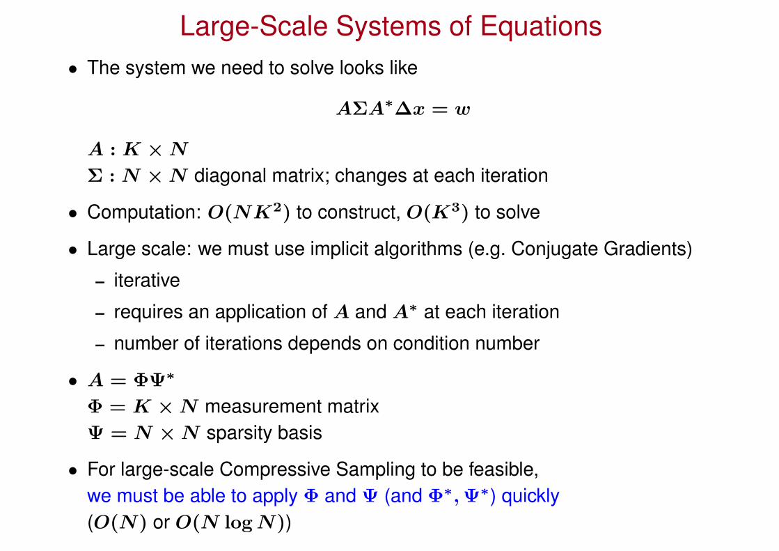
Large-Scale Systems of Equations• The system we need to solve looks like
AΣA∗∆x = w
A : K × N
Σ : N × N diagonal matrix; changes at each iteration
• Computation: O(NK2) to construct, O(K3) to solve
• Large scale: we must use implicit algorithms (e.g. Conjugate Gradients)
– iterative
– requires an application of A and A∗ at each iteration
– number of iterations depends on condition number
• A = ΦΨ∗
Φ = K × N measurement matrixΨ = N × N sparsity basis
• For large-scale Compressive Sampling to be feasible,we must be able to apply Φ and Ψ (and Φ∗, Ψ∗) quickly(O(N) or O(N log N))
Fast Measurements
• Say we want to take 20, 000 measurements of a 512 × 512 image(N = 262, 144)
• If Φ is Gaussian, with each entry a float, it would take more than an entireDVD just to hold Φ
• Need fast, implicit, noise-like measurement systems to make recoveryfeasible
• Partial Fourier ensemble is O(N log N) (FFT and subsample)
• Tomography: many fast unequispaced Fourier transforms,Dutt and Rohklin, Pseudopolar FFT of Averbuch et. al
• Noiselet system of Coifman and Meyer
– perfectly incoherent with Haar system
– performs the same as Gaussian (in numerical experiments) forrecovering spikes and sparse Haar signals
– O(N)
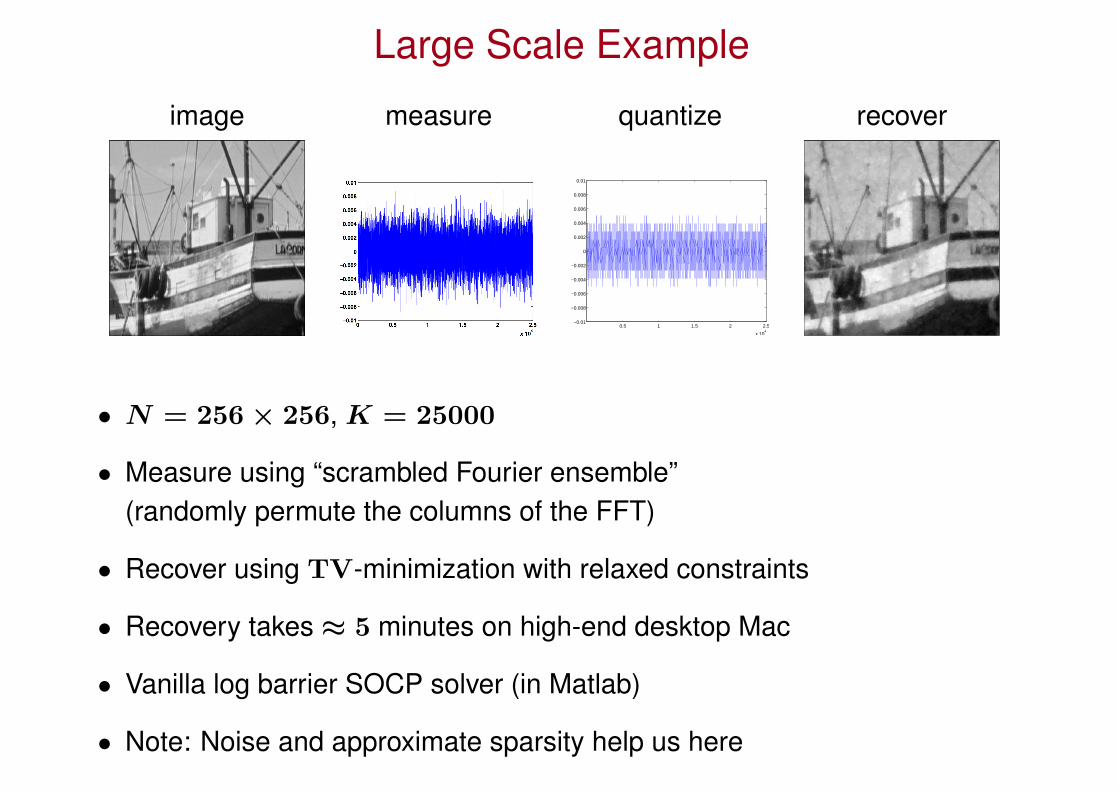
Large Scale Example
image measure quantize recover
0.5 1 1.5 2 2.5
x 104
−0.01
−0.008
−0.006
−0.004
−0.002
0
0.002
0.004
0.006
0.008
0.01
• N = 256 × 256, K = 25000
• Measure using “scrambled Fourier ensemble”(randomly permute the columns of the FFT)
• Recover using TV-minimization with relaxed constraints
• Recovery takes ≈ 5 minutes on high-end desktop Mac
• Vanilla log barrier SOCP solver (in Matlab)
• Note: Noise and approximate sparsity help us here
Compressive Sampling in Noisy Environments
ICIP Tutorial, 2006 Robert Nowak, www.ece.wisc.edu/~nowak
Convention: Oversample and then remove redundancy to extract information
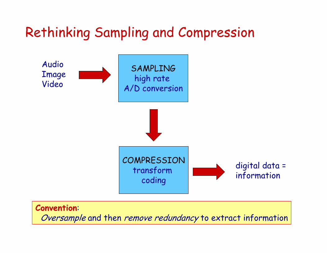
Rethinking Sampling and Compression
AudioImageVideo
SAMPLINGhigh rate
A/D conversion
COMPRESSIONtransform
coding
digital data = information
Convention: Oversample and then remove redundancy to extract information
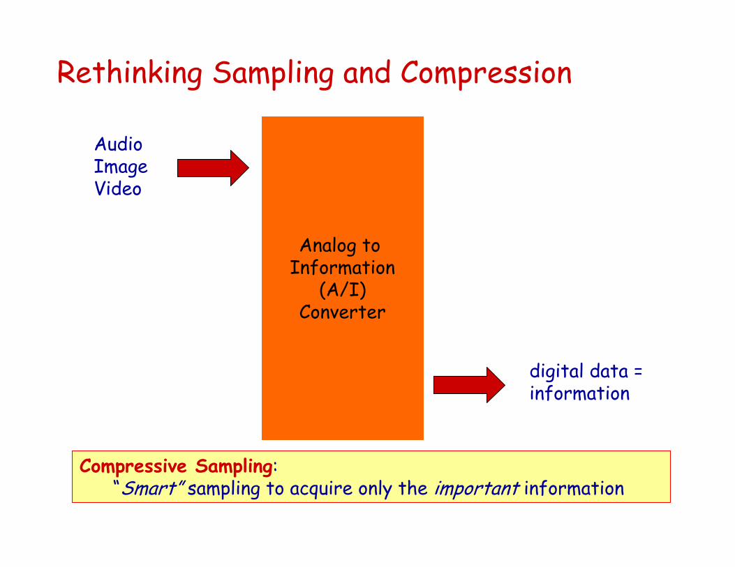
Compressive Sampling: “Smart” sampling to acquire only the important information
Rethinking Sampling and Compression
AudioImageVideo
SAMPLINGhigh rate
A/D conversion
COMPRESSIONtransform
coding
digital data = information
Analog to Information
(A/I)Converter
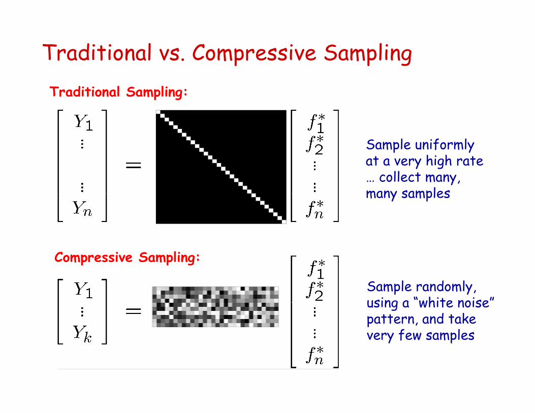
Traditional vs. Compressive SamplingTraditional Sampling:
Sample uniformly at a very high rate … collect many, many samples
Compressive Sampling:
Sample randomly, using a “white noise” pattern, and take very few samples
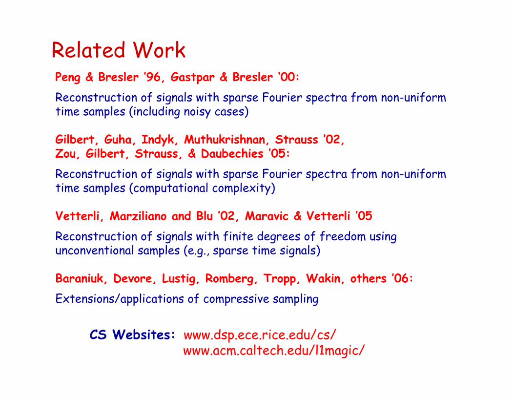
Related WorkPeng & Bresler ’96, Gastpar & Bresler ‘00:Reconstruction of signals with sparse Fourier spectra from non-uniform time samples (including noisy cases)
Gilbert, Guha, Indyk, Muthukrishnan, Strauss ’02,Zou, Gilbert, Strauss, & Daubechies ’05:Reconstruction of signals with sparse Fourier spectra from non-uniform time samples (computational complexity)
Vetterli, Marziliano and Blu ’02, Maravic & Vetterli ’05Reconstruction of signals with finite degrees of freedom using unconventional samples (e.g., sparse time signals)
Baraniuk, Devore, Lustig, Romberg, Tropp, Wakin, others ’06:Extensions/applications of compressive sampling
CS Websites: www.dsp.ece.rice.edu/cs/www.acm.caltech.edu/l1magic/
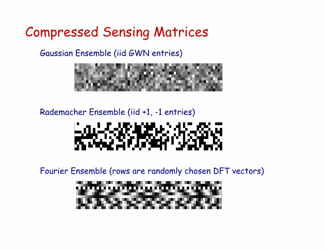
Gaussian Ensemble (iid GWN entries)
Rademacher Ensemble (iid +1, -1 entries)
Fourier Ensemble (rows are randomly chosen DFT vectors)
Compressed Sensing Matrices
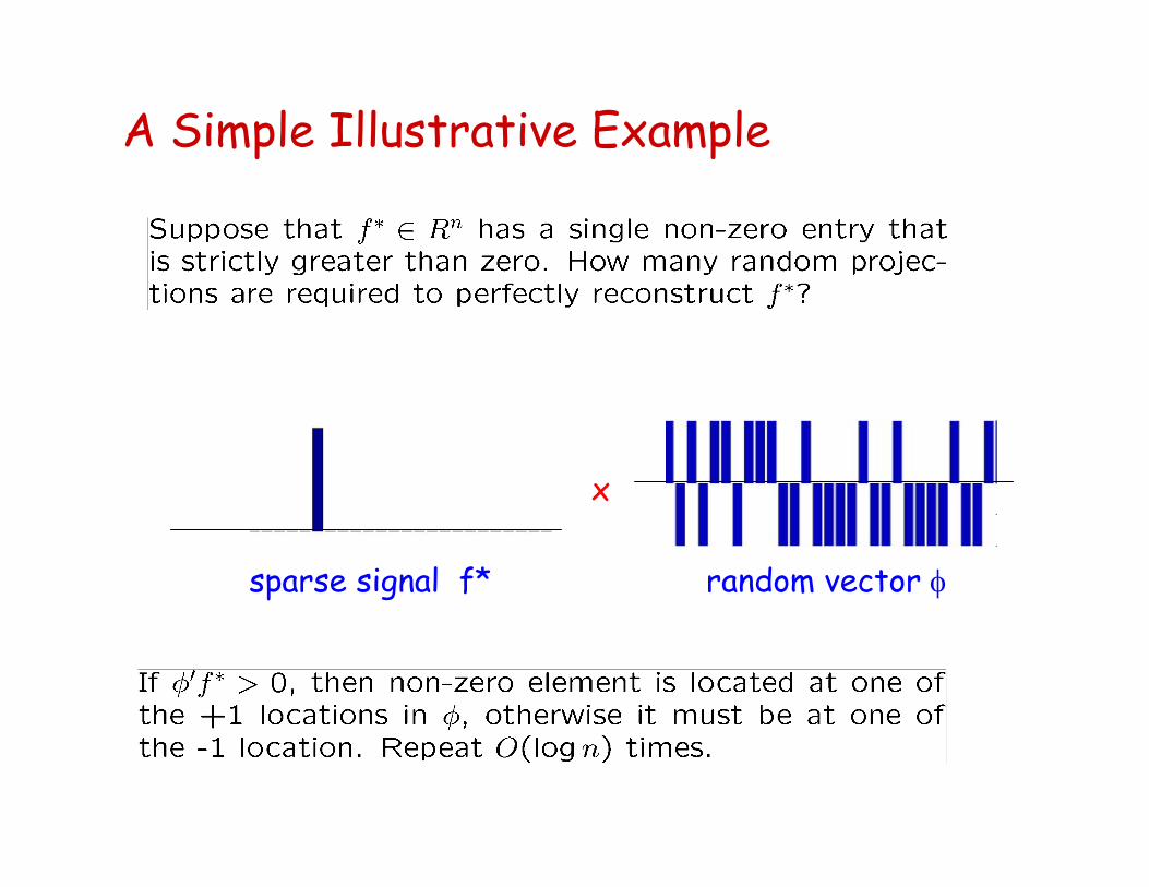
A Simple Illustrative Example
x
sparse signal f* random vector φ
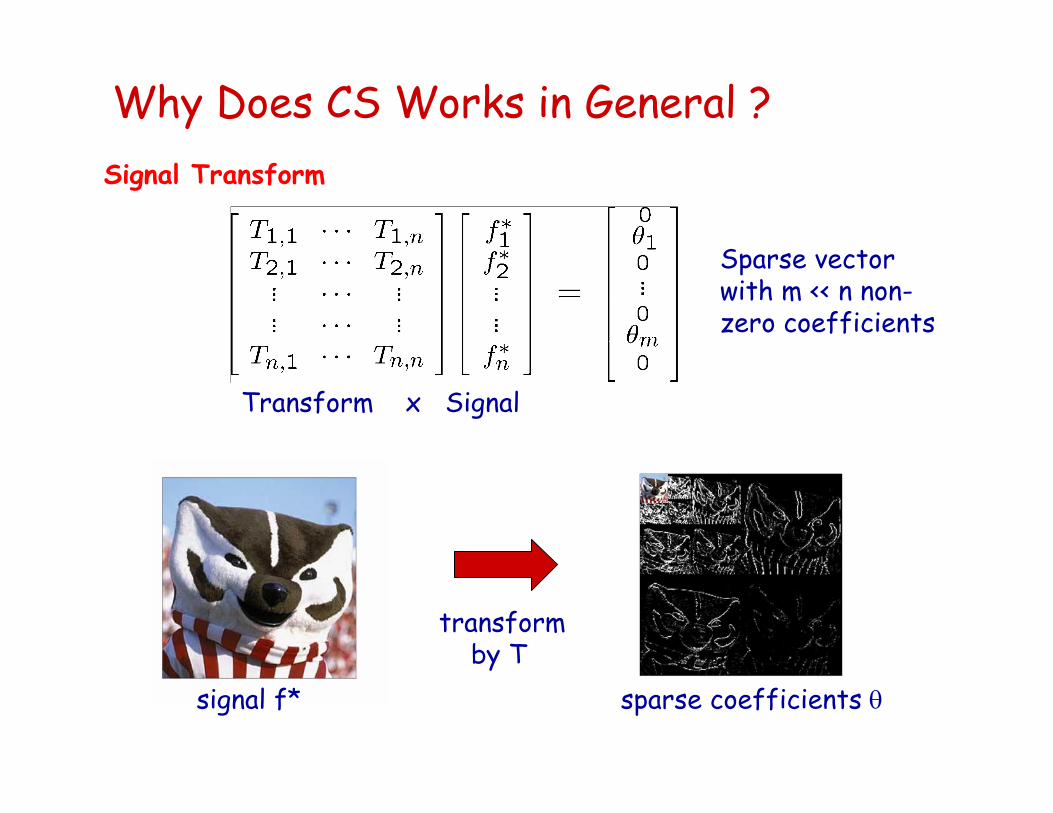
Why Does CS Works in General ?
Transform x Signal
Sparse vector with m << n non-zero coefficients
Signal Transform
transform by T
signal f* sparse coefficients θ
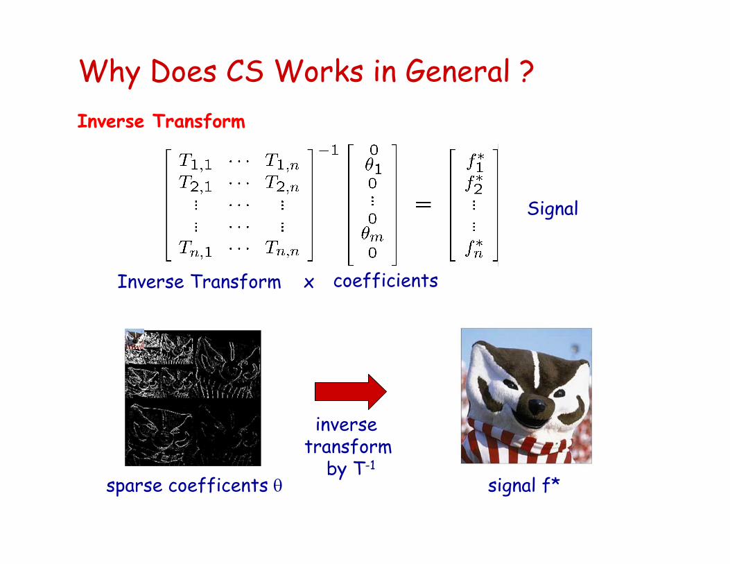
Why Does CS Works in General ?
Inverse Transform x
Signal
Inverse Transform
inverse transform
by T-1
signal f*sparse coefficents θ
coefficients
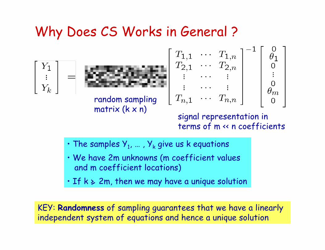
random sampling matrix (k x n)
signal representation in terms of m << n coefficients
• The samples Y1, … , Yk give us k equations• We have 2m unknowns (m coefficient values
and m coefficient locations)• If k > 2m, then we may have a unique solution
KEY: Randomness of sampling guarantees that we have a linearly independent system of equations and hence a unique solution
Why Does CS Works in General ?
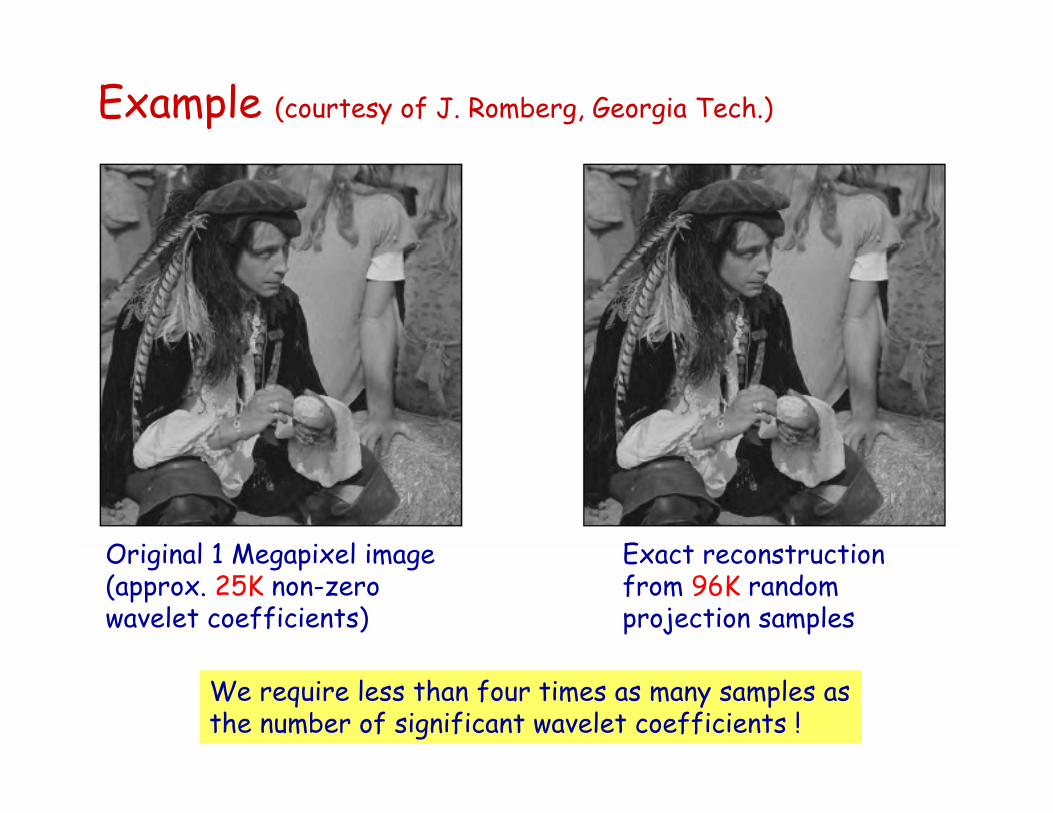
Example (courtesy of J. Romberg, Georgia Tech.)
Original 1 Megapixel image(approx. 25K non-zero wavelet coefficients)
Exact reconstruction from 96K random projection samples
We require less than four times as many samples as the number of significant wavelet coefficients !
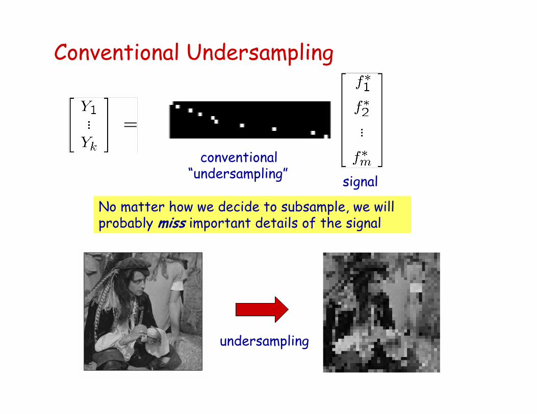
Conventional Undersampling
conventional “undersampling” signal
No matter how we decide to subsample, we will probably miss important details of the signal
undersampling
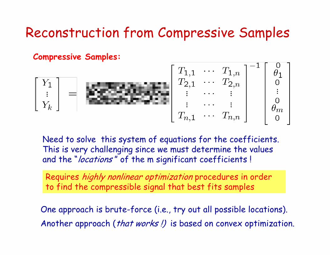
Reconstruction from Compressive SamplesCompressive Samples:
Need to solve this system of equations for the coefficients. This is very challenging since we must determine the values and the “locations ” of the m significant coefficients !
Requires highly nonlinear optimization procedures in order to find the compressible signal that best fits samples
One approach is brute-force (i.e., try out all possible locations).Another approach (that works !) is based on convex optimization.
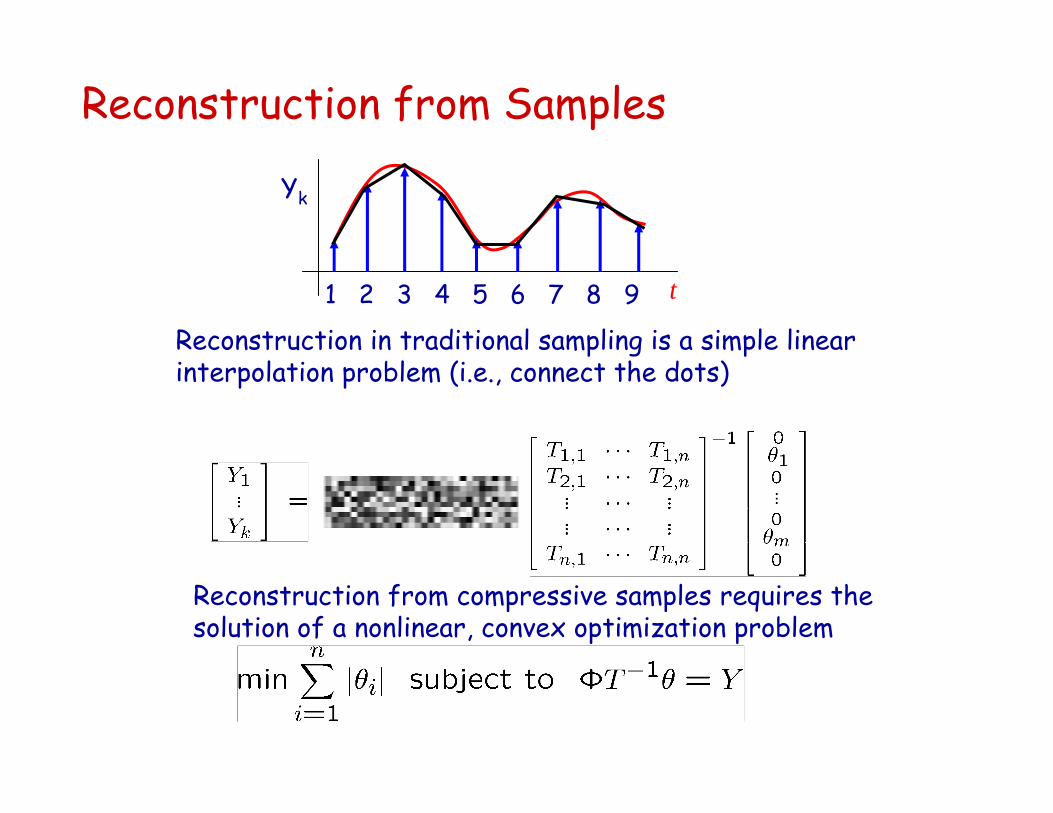
Reconstruction from Samples
1 2 3 4 5 6 7 8 9 t
Reconstruction in traditional sampling is a simple linear interpolation problem (i.e., connect the dots)
Yk
Reconstruction from compressive samples requires the solution of a nonlinear, convex optimization problem
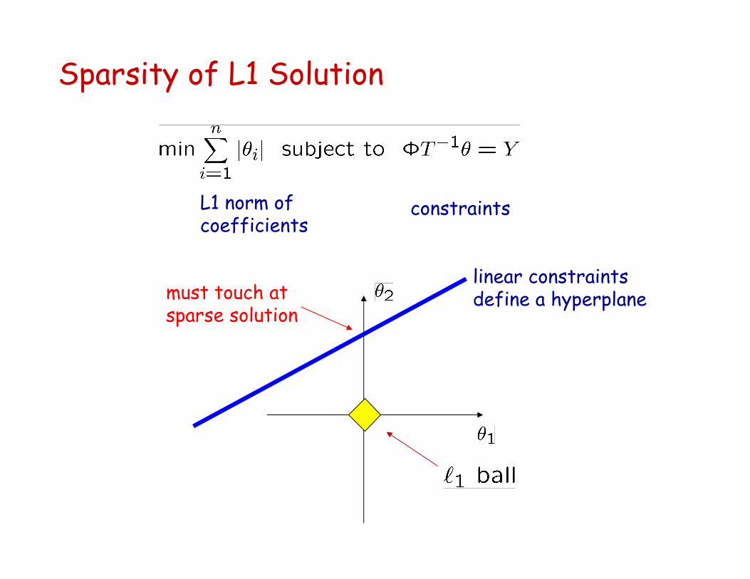
Sparsity of L1 Solution
linear constraints define a hyperplanemust touch at
sparse solution
constraintsL1 norm of coefficients
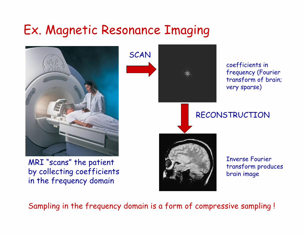
Ex. Magnetic Resonance Imaging
MRI “scans” the patient by collecting coefficients in the frequency domain
SCANcoefficients in frequency (Fourier transform of brain; very sparse)
Inverse Fourier transform produces brain image
RECONSTRUCTION
Sampling in the frequency domain is a form of compressive sampling !
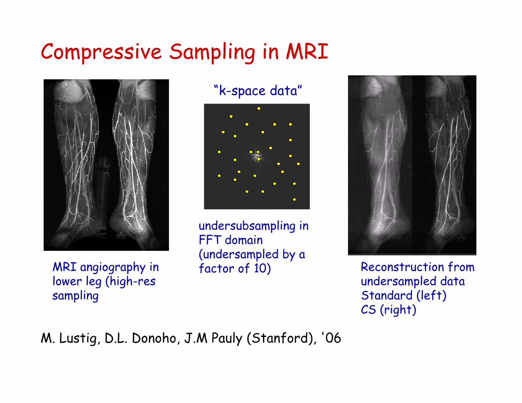
Compressive Sampling in MRI
M. Lustig, D.L. Donoho, J.M Pauly (Stanford), '06
MRI angiography in lower leg (high-ressampling
undersubsampling in FFT domain (undersampled by a factor of 10) Reconstruction from
undersampled dataStandard (left)CS (right)
“k-space data”
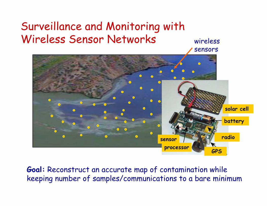
Goal: Reconstruct an accurate map of contamination while keeping number of samples/communications to a bare minimum
Surveillance and Monitoring withWireless Sensor Networks wireless
sensors
sensorprocessor
GPS
radio
battery
solar cell
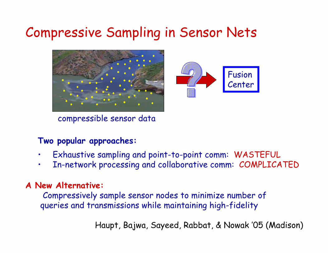
Compressive Sampling in Sensor Nets
Fusion Center
compressible sensor data
Two popular approaches:• Exhaustive sampling and point-to-point comm: WASTEFUL• In-network processing and collaborative comm: COMPLICATED
A New Alternative:Compressively sample sensor nodes to minimize number of
queries and transmissions while maintaining high-fidelity
Haupt, Bajwa, Sayeed, Rabbat, & Nowak ’05 (Madison)
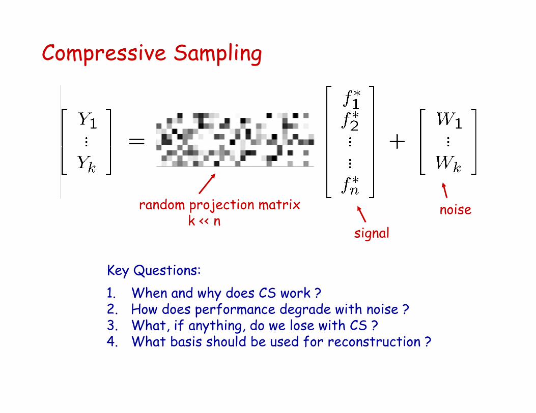
Compressive Sampling
signal
random projection matrixk << n
Key Questions:1. When and why does CS work ?2. How does performance degrade with noise ?3. What, if anything, do we lose with CS ?4. What basis should be used for reconstruction ?
noise
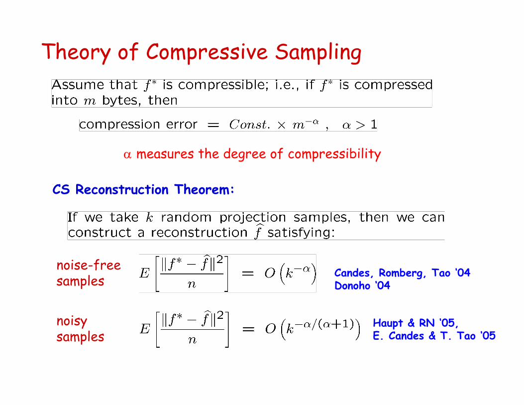
Theory of Compressive Sampling
Candes, Romberg, Tao ‘04Donoho ‘04
Haupt & RN ‘05, E. Candes & T. Tao ‘05
CS Reconstruction Theorem:
α measures the degree of compressibility
noise-free samples
noisy samples
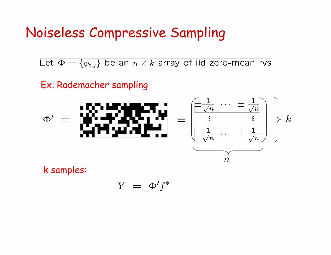
Noiseless Compressive Sampling
Ex. Rademacher sampling
k samples:
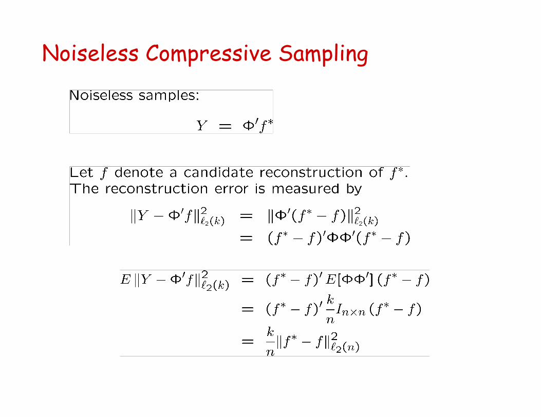
Noiseless Compressive Sampling
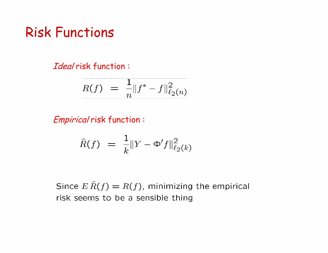
Risk Functions
Ideal risk function :
Empirical risk function :
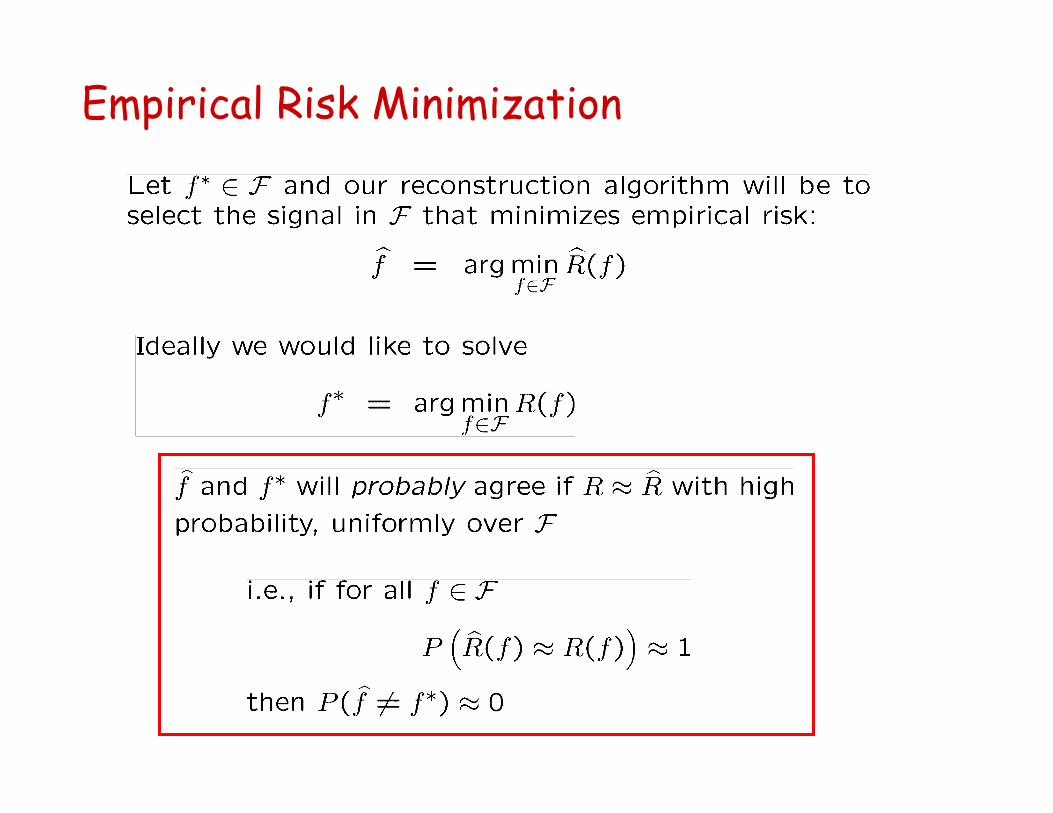
Empirical Risk Minimization
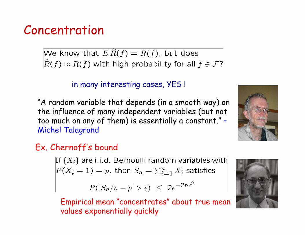
Concentration
in many interesting cases, YES !
“A random variable that depends (in a smooth way) on the influence of many independent variables (but not too much on any of them) is essentially a constant.” –Michel Talagrand
Ex. Chernoff’s bound
Empirical mean “concentrates” about true mean values exponentially quickly
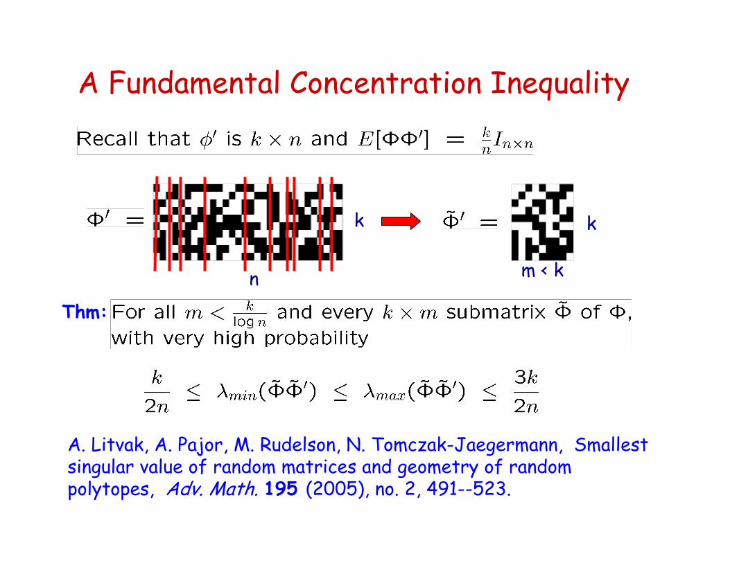
A Fundamental Concentration Inequality
A. Litvak, A. Pajor, M. Rudelson, N. Tomczak-Jaegermann, Smallest singular value of random matrices and geometry of random polytopes, Adv. Math. 195 (2005), no. 2, 491--523.
Thm:
n
k k
m < k
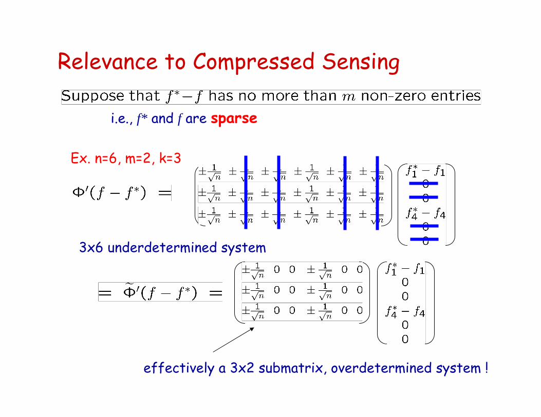
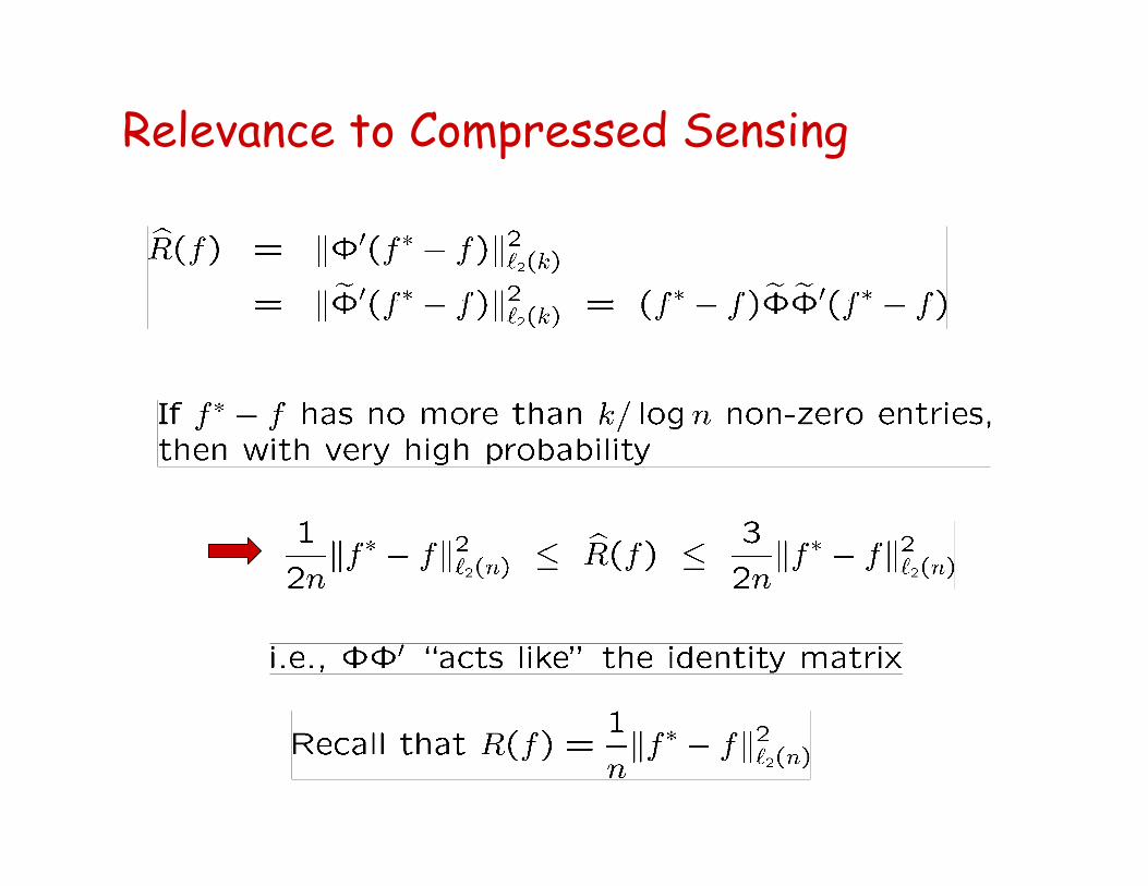
Relevance to Compressed Sensing
Ex. n=6, m=2, k=3
i.e., f* and f are sparse
effectively a 3x2 submatrix, overdetermined system !
3x6 underdetermined system
Relevance to Compressed Sensing
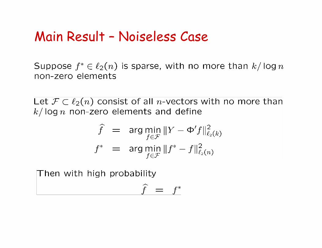
Main Result – Noiseless Case
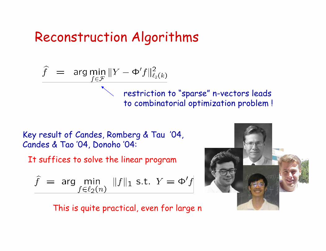
Reconstruction Algorithms
restriction to “sparse” n-vectors leads to combinatorial optimization problem !
Key result of Candes, Romberg & Tau ’04, Candes & Tao ’04, Donoho ’04:
It suffices to solve the linear program
This is quite practical, even for large n
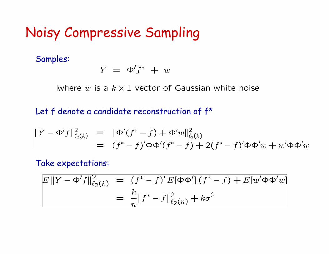
Noisy Compressive Sampling
Samples:
Let f denote a candidate reconstruction of f*
Take expectations:
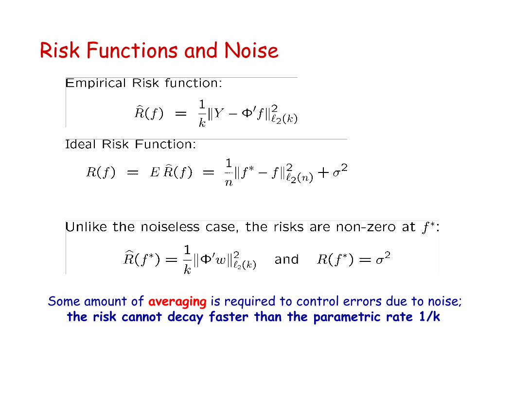
Risk Functions and Noise
Some amount of averaging is required to control errors due to noise; the risk cannot decay faster than the parametric rate 1/k
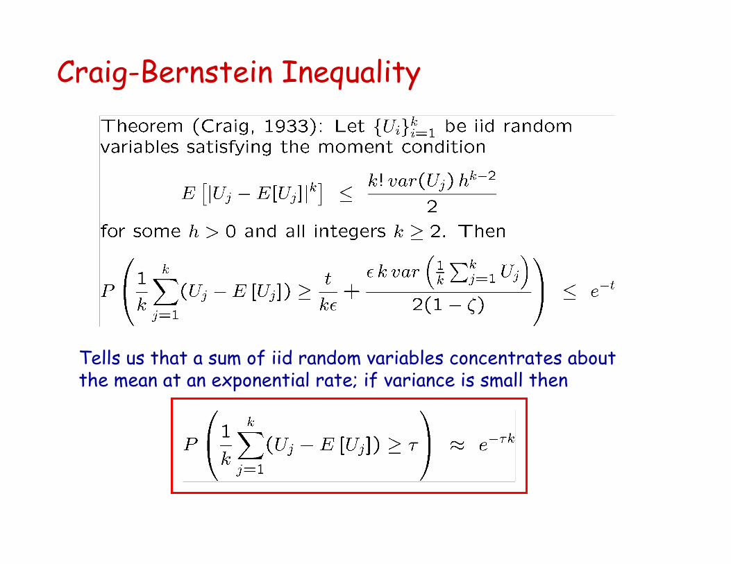
Craig-Bernstein Inequality
Tells us that a sum of iid random variables concentrates about the mean at an exponential rate; if variance is small then
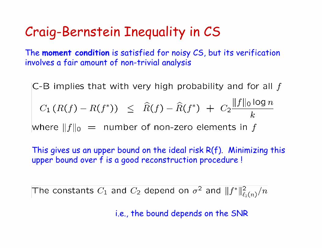
Craig-Bernstein Inequality in CSThe moment condition is satisfied for noisy CS, but its verification involves a fair amount of non-trivial analysis
i.e., the bound depends on the SNR
This gives us an upper bound on the ideal risk R(f). Minimizing this upper bound over f is a good reconstruction procedure !
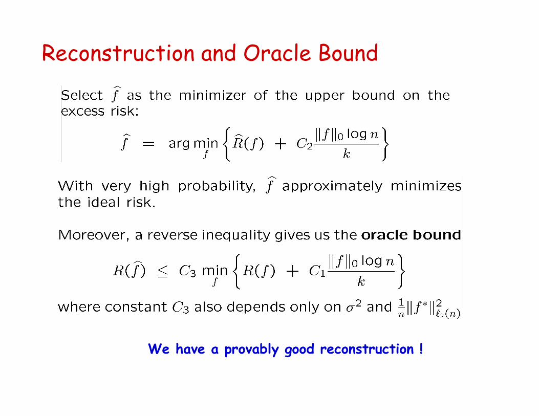
Reconstruction and Oracle Bound
We have a provably good reconstruction !
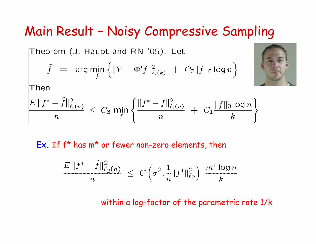
Main Result – Noisy Compressive Sampling
Ex. If f* has m* or fewer non-zero elements, then
within a log-factor of the parametric rate 1/k
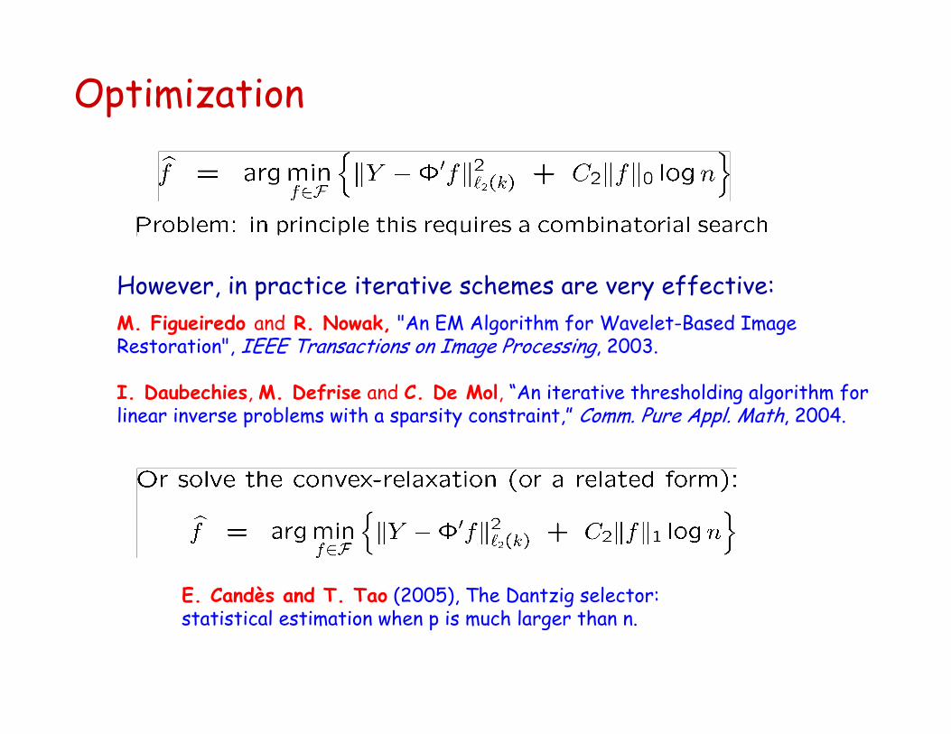
Optimization
However, in practice iterative schemes are very effective:M. Figueiredo and R. Nowak, "An EM Algorithm for Wavelet-Based Image Restoration", IEEE Transactions on Image Processing, 2003.
I. Daubechies, M. Defrise and C. De Mol, “An iterative thresholding algorithm for linear inverse problems with a sparsity constraint,” Comm. Pure Appl. Math, 2004.
E. Candès and T. Tao (2005), The Dantzig selector: statistical estimation when p is much larger than n.
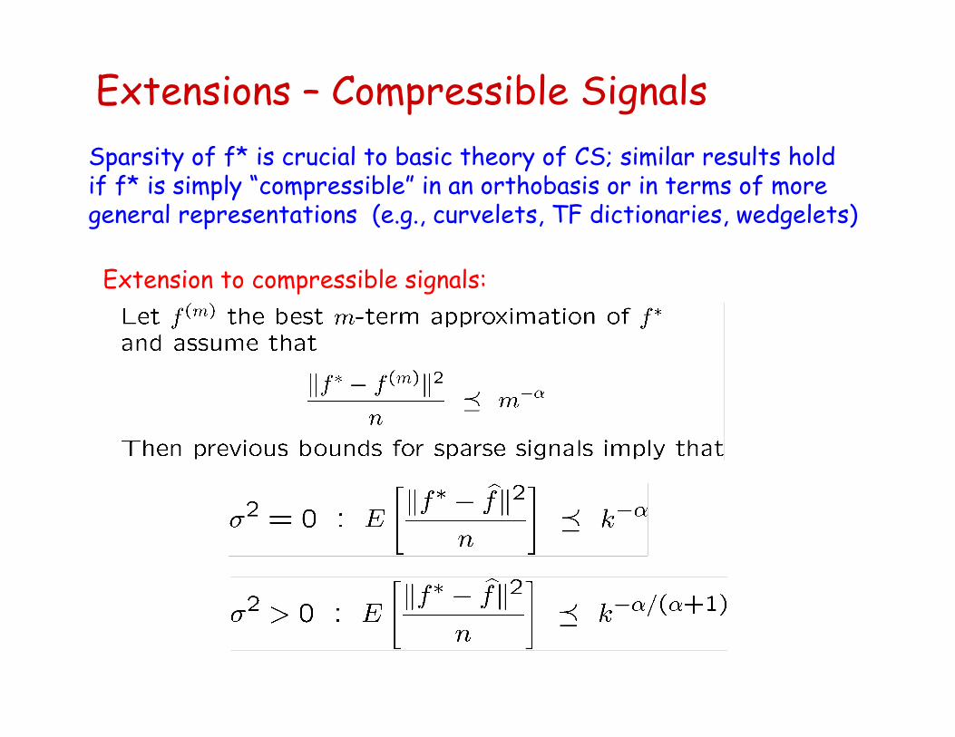
Extensions – Compressible SignalsSparsity of f* is crucial to basic theory of CS; similar results hold if f* is simply “compressible” in an orthobasis or in terms of more general representations (e.g., curvelets, TF dictionaries, wedgelets)
Extension to compressible signals:
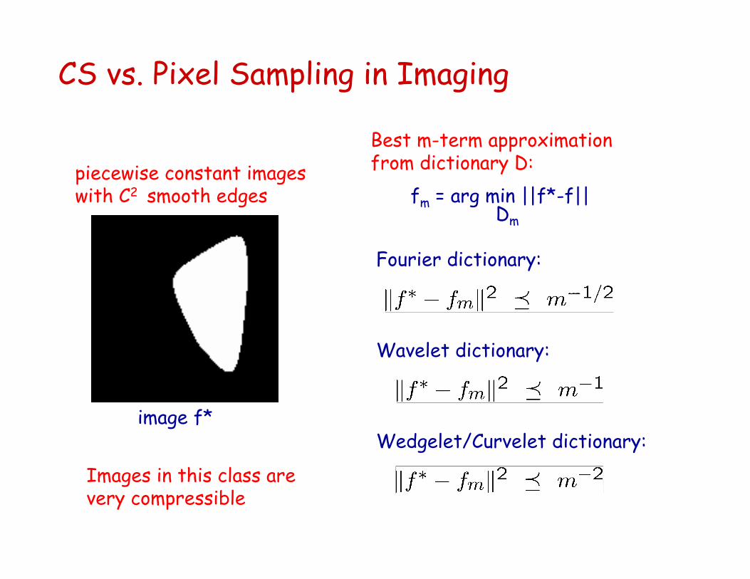
CS vs. Pixel Sampling in Imaging
piecewise constant images with C2 smooth edges
image f*
Best m-term approximation from dictionary D:
fm = arg min ||f*-f||Dm
Fourier dictionary:
Wavelet dictionary:
Wedgelet/Curvelet dictionary:
Images in this class arevery compressible
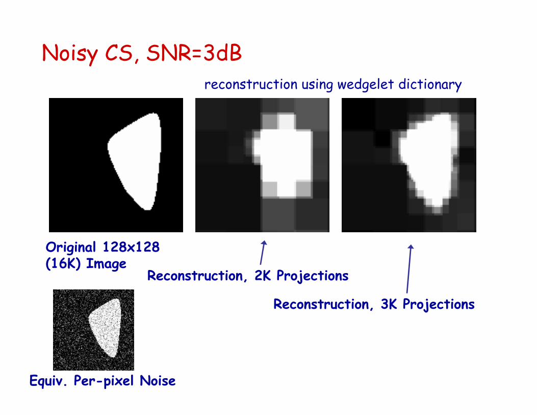
Noisy CS, SNR=3dB
Original 128x128 (16K) Image
Reconstruction, 2K Projections
Reconstruction, 3K Projections
reconstruction using wedgelet dictionary
Equiv. Per-pixel Noise
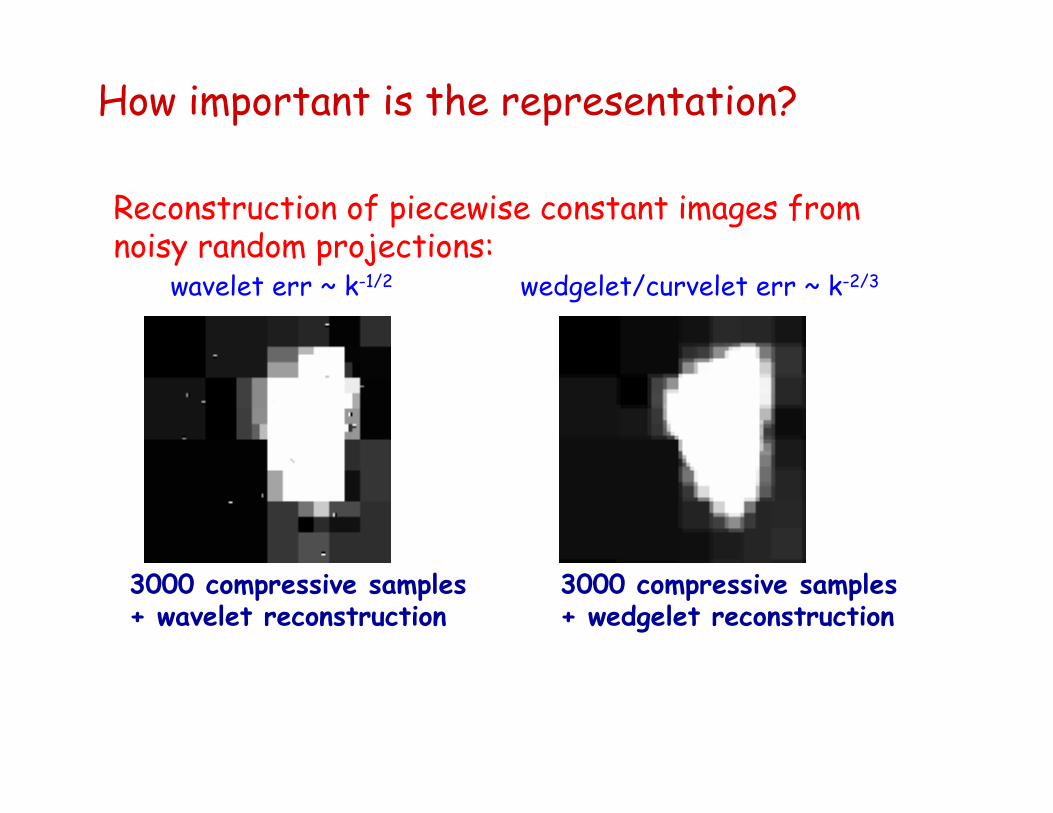
How important is the representation?
Reconstruction of piecewise constant images from noisy random projections:
wavelet err ~ k-1/2 wedgelet/curvelet err ~ k-2/3
3000 compressive samples + wedgelet reconstruction
3000 compressive samples + wavelet reconstruction
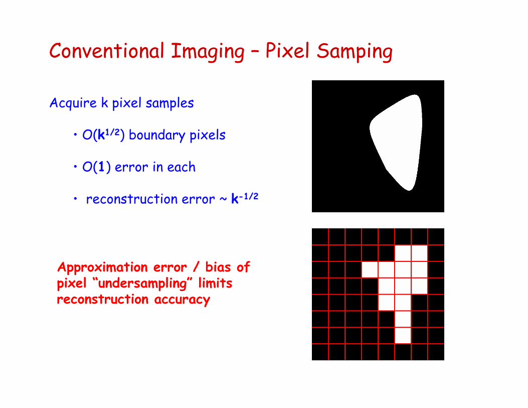
Conventional Imaging – Pixel Samping
Acquire k pixel samples
• O(k1/2) boundary pixels
• O(1) error in each
• reconstruction error ~ k-1/2
Approximation error / bias of pixel “undersampling” limits reconstruction accuracy
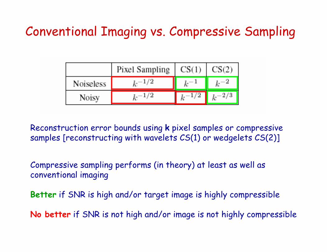
Conventional Imaging vs. Compressive Sampling
Reconstruction error bounds using k pixel samples or compressive samples [reconstructing with wavelets CS(1) or wedgelets CS(2)]
Compressive sampling performs (in theory) at least as well as conventional imaging
Better if SNR is high and/or target image is highly compressible
No better if SNR is not high and/or image is not highly compressible
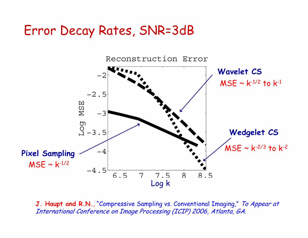
Error Decay Rates, SNR=3dB
Pixel Sampling
Wavelet CS
Wedgelet CS
J. Haupt and R.N., “Compressive Sampling vs. Conventional Imaging,” To Appear at International Conference on Image Processing (ICIP) 2006, Atlanta, GA.
MSE ~ k-1/2
MSE ~ k-1/2 to k-1
MSE ~ k-2/3 to k-2
Log k
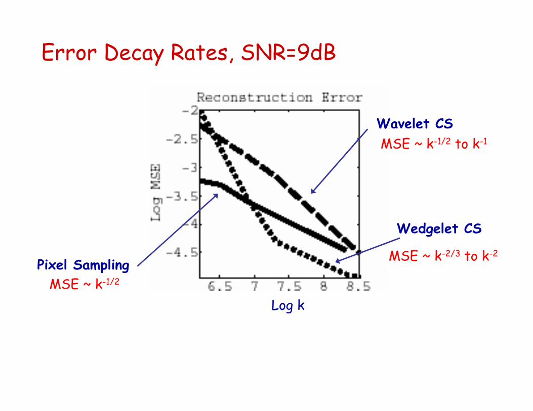
Error Decay Rates, SNR=9dB
Pixel Sampling
Wavelet CS
Wedgelet CS
MSE ~ k-1/2
MSE ~ k-1/2 to k-1
MSE ~ k-2/3 to k-2
Log k
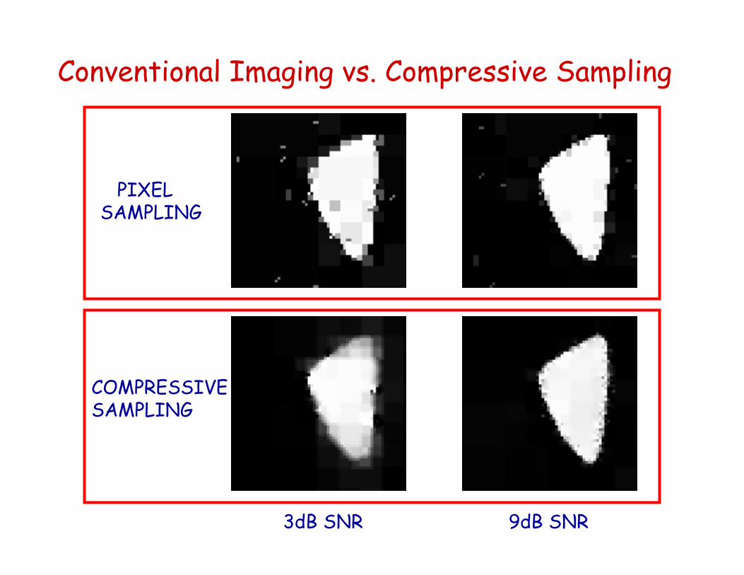
Conventional Imaging vs. Compressive Sampling
PIXEL SAMPLING
COMPRESSIVE SAMPLING
3dB SNR 9dB SNR
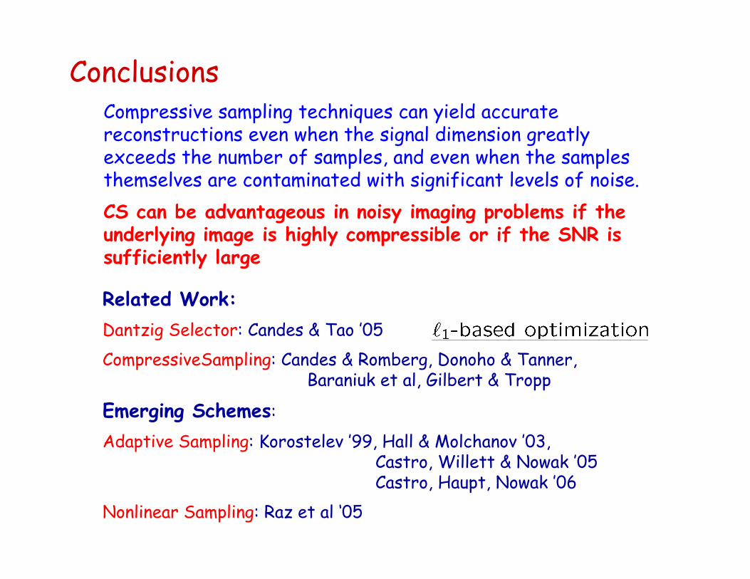
ConclusionsCompressive sampling techniques can yield accurate reconstructions even when the signal dimension greatly exceeds the number of samples, and even when the samples themselves are contaminated with significant levels of noise.CS can be advantageous in noisy imaging problems if the underlying image is highly compressible or if the SNR is sufficiently large
Related Work:Dantzig Selector: Candes & Tao ’05 CompressiveSampling: Candes & Romberg, Donoho & Tanner,
Baraniuk et al, Gilbert & Tropp
Emerging Schemes:Adaptive Sampling: Korostelev ’99, Hall & Molchanov ’03,
Castro, Willett & Nowak ’05Castro, Haupt, Nowak ’06
Nonlinear Sampling: Raz et al ‘05
Adaptive Sampling
x
x
x
x
x
x
x x
x
x
x
x
x
x xx
x
x
x
x
x
x
x
x
xx
x
x
x x
x xx
x
x
x x
x
xx
x
x
x
x
x
x
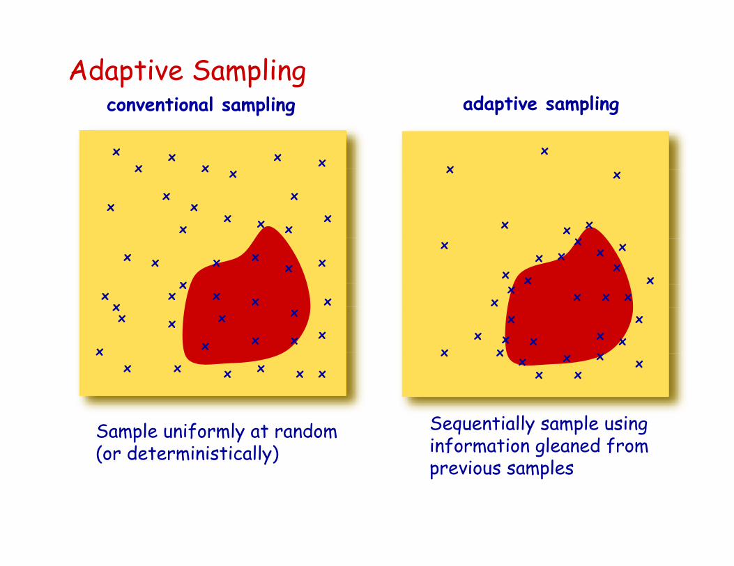
Sequentially sample using information gleaned from previous samples
x
x
x
x
x
x
x
x
xx
xx
xxx
x
xx
xx
xx
x
x
x
x
x
xx
xx
x
Sample uniformly at random (or deterministically)
conventional sampling adaptive sampling
x
x
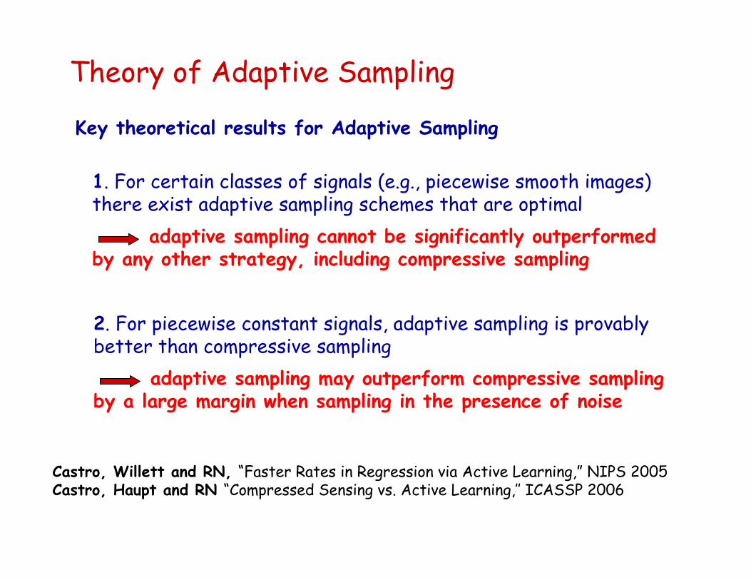
Theory of Adaptive Sampling
1. For certain classes of signals (e.g., piecewise smooth images)there exist adaptive sampling schemes that are optimal
adaptive sampling cannot be significantly outperformed by any other strategy, including compressive sampling
2. For piecewise constant signals, adaptive sampling is provably better than compressive sampling
adaptive sampling may outperform compressive sampling by a large margin when sampling in the presence of noise
Key theoretical results for Adaptive Sampling
Castro, Willett and RN, “Faster Rates in Regression via Active Learning,” NIPS 2005Castro, Haupt and RN “Compressed Sensing vs. Active Learning,’’ ICASSP 2006
50 100 150 200 250
50
100
150
200
25050 100 150 200 250
50
100
150
200
25050 100 150 200 250
50
100
150
200
25020 40 60 80 100 120
20
40
60
80
100
120
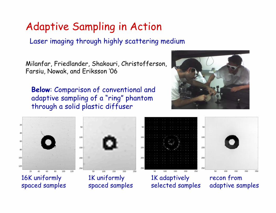
16K uniformly spaced samples
1K uniformly spaced samples
1K adaptively selected samples
recon from adaptive samples
Adaptive Sampling in ActionLaser imaging through highly scattering medium
Below: Comparison of conventional and adaptive sampling of a “ring” phantom through a solid plastic diffuser
Milanfar, Friedlander, Shakouri, Christofferson, Farsiu, Nowak, and Eriksson ‘06
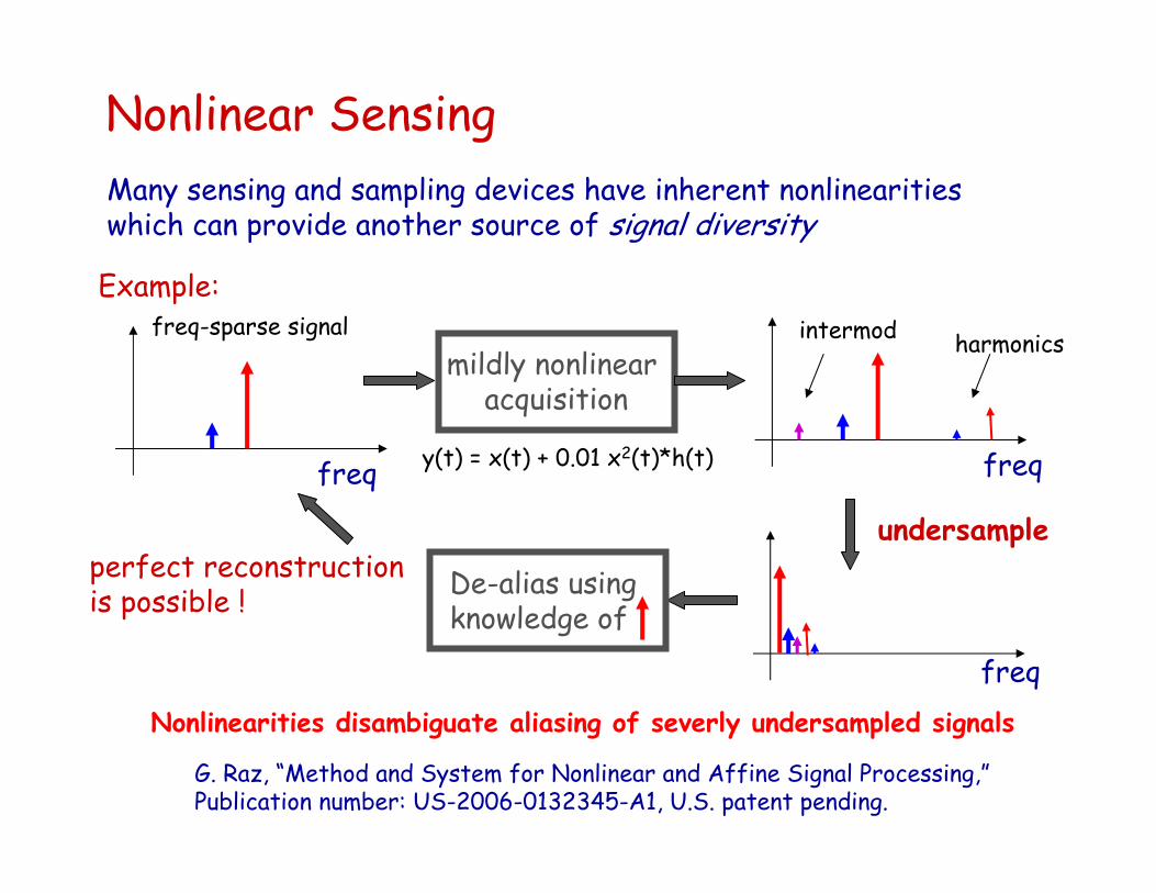
Nonlinear SensingMany sensing and sampling devices have inherent nonlinearities which can provide another source of signal diversity
Example:
freq
mildly nonlinear acquisition
freq
harmonicsintermod
undersample
freq
De-alias using knowledge of
perfect reconstructionis possible !
freq-sparse signal
Nonlinearities disambiguate aliasing of severly undersampled signals
y(t) = x(t) + 0.01 x2(t)*h(t)
G. Raz, “Method and System for Nonlinear and Affine Signal Processing,”Publication number: US-2006-0132345-A1, U.S. patent pending.
26-29 August 2007 Madison, Wisconsin
General Chairs: R. Nowak & H. KrimTech Chairs: R. Baraniuk and A. Sayeed
Biosignal processing and medical imaging Time-frequency and time-scale analysis
New methods, directions and applications. System identification and calibration
Information forensics and security Multivariate statistical analysis
Sensor networks Learning theory and pattern recognition
Communication systems and networks Distributed signal processing
Array processing, radar and sonar Detection and estimation theory
Automotive and industrial applicationsMonte Carlo methods
Bioinformatics and genomic signal processing Adaptive systems and signal processing
Application areasTheoretical topics
2007 IEEE Statistical Signal Processing Workshop

Part IV –Applications
and Wrapup
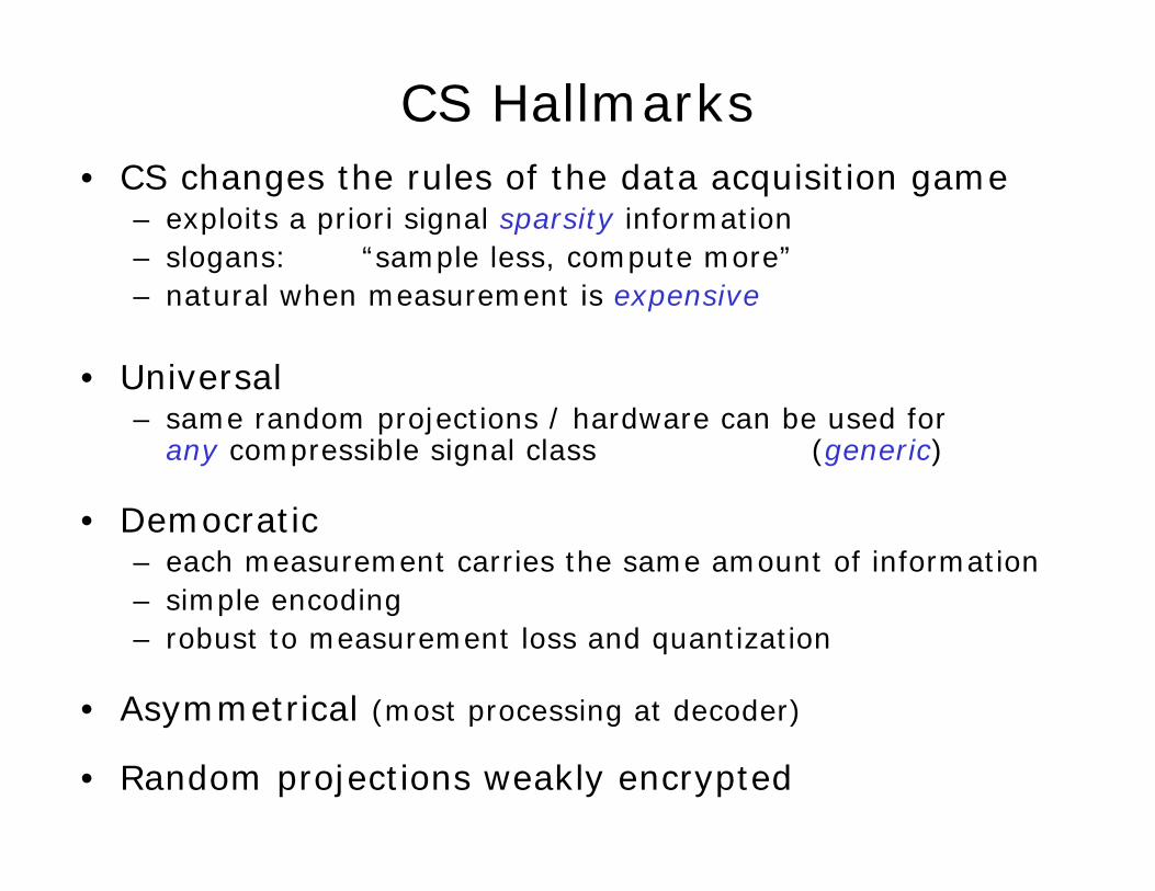
CS Hallmarks• CS changes the rules of the data acquisition game
– exploits a priori signal sparsity information – slogans: “sample less, compute more”– natural when measurement is expensive
• Universal – same random projections / hardware can be used for
any compressible signal class (generic)
• Democratic– each measurement carries the same amount of information– simple encoding– robust to measurement loss and quantization
• Asymmetrical (most processing at decoder)
• Random projections weakly encrypted
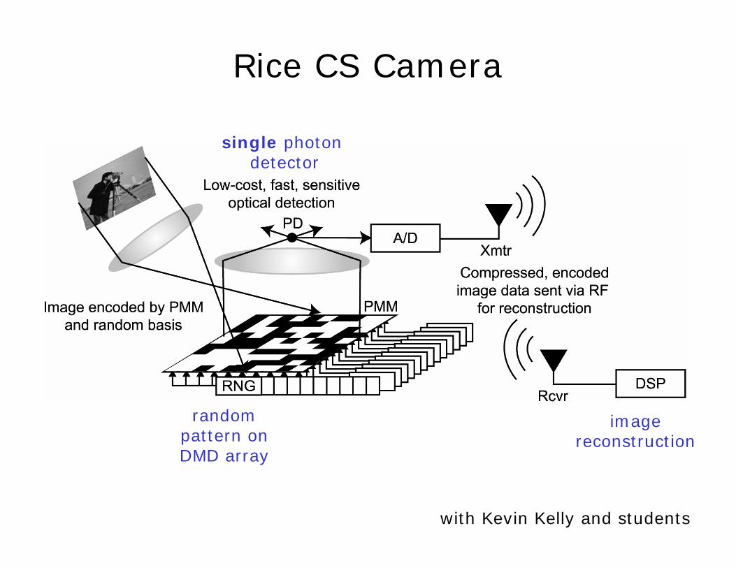
Rice CS Camera
single photon detector
randompattern onDMD array
imagereconstruction
with Kevin Kelly and students
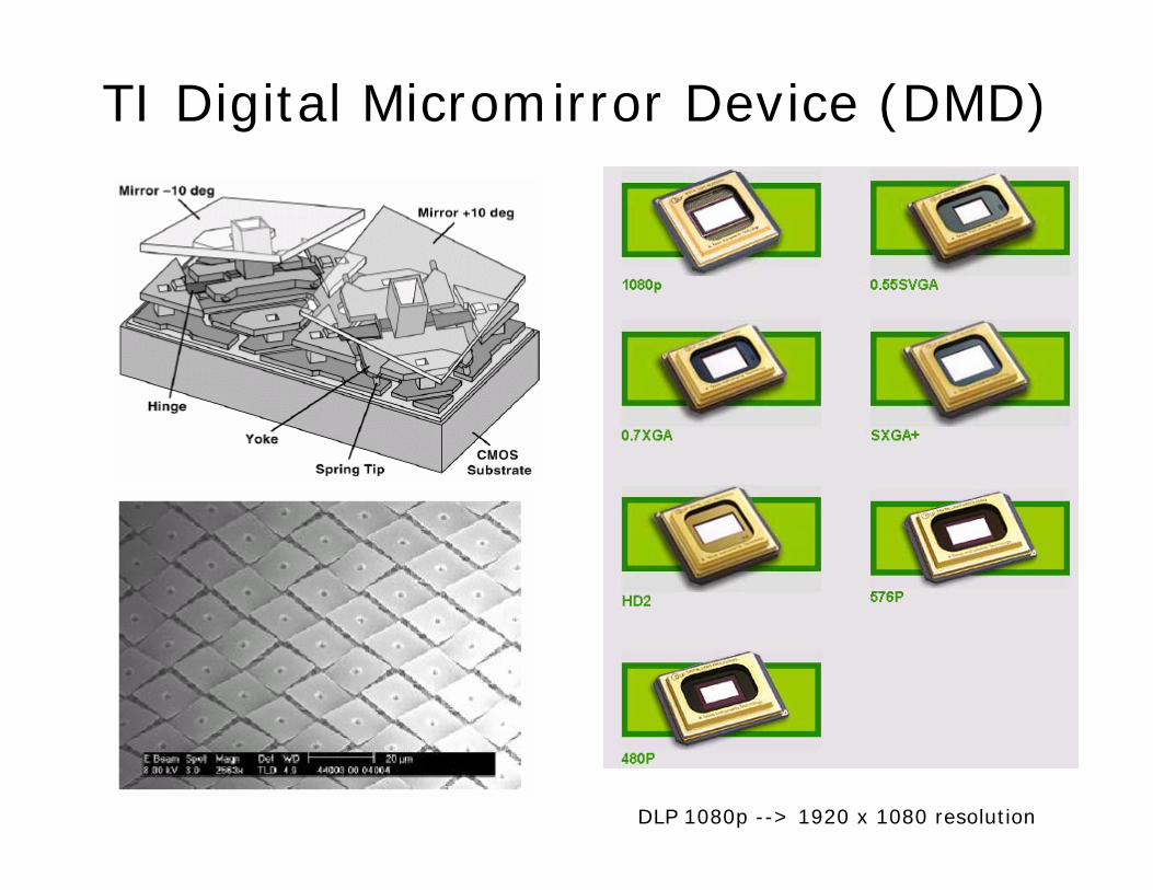
TI Digital Micromirror Device (DMD)
DLP 1080p --> 1920 x 1080 resolution
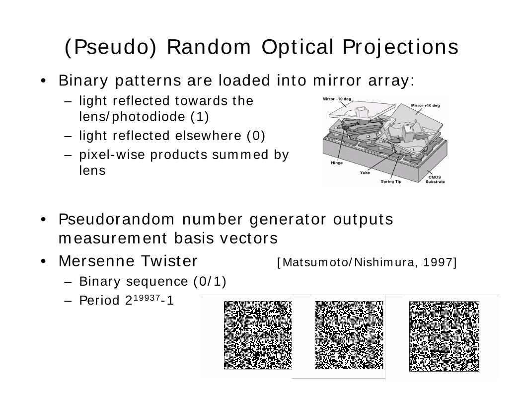
(Pseudo) Random Optical Projections
• Pseudorandom number generator outputs measurement basis vectors
• Mersenne Twister [Matsumoto/Nishimura, 1997]
– Binary sequence (0/1)– Period 219937-1 …
• Binary patterns are loaded into mirror array: – light reflected towards the
lens/photodiode (1) – light reflected elsewhere (0)– pixel-wise products summed by
lens
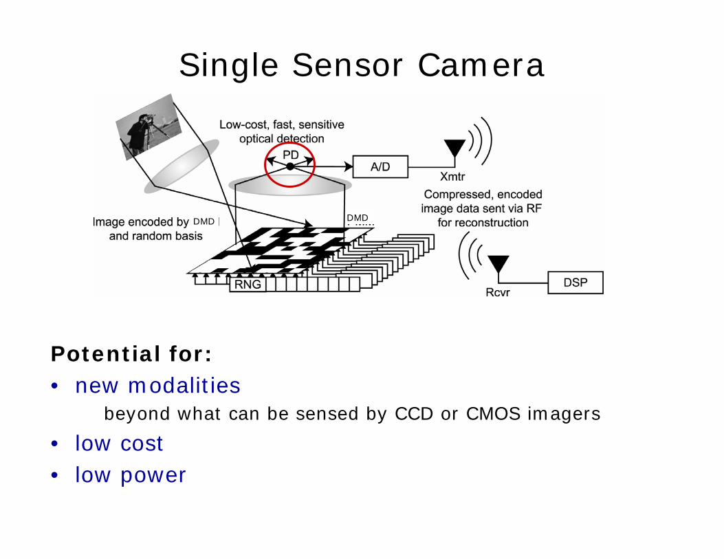
Single Sensor Camera
Potential for:• new modalities
beyond what can be sensed by CCD or CMOS imagers
• low cost• low power
DMD DMD
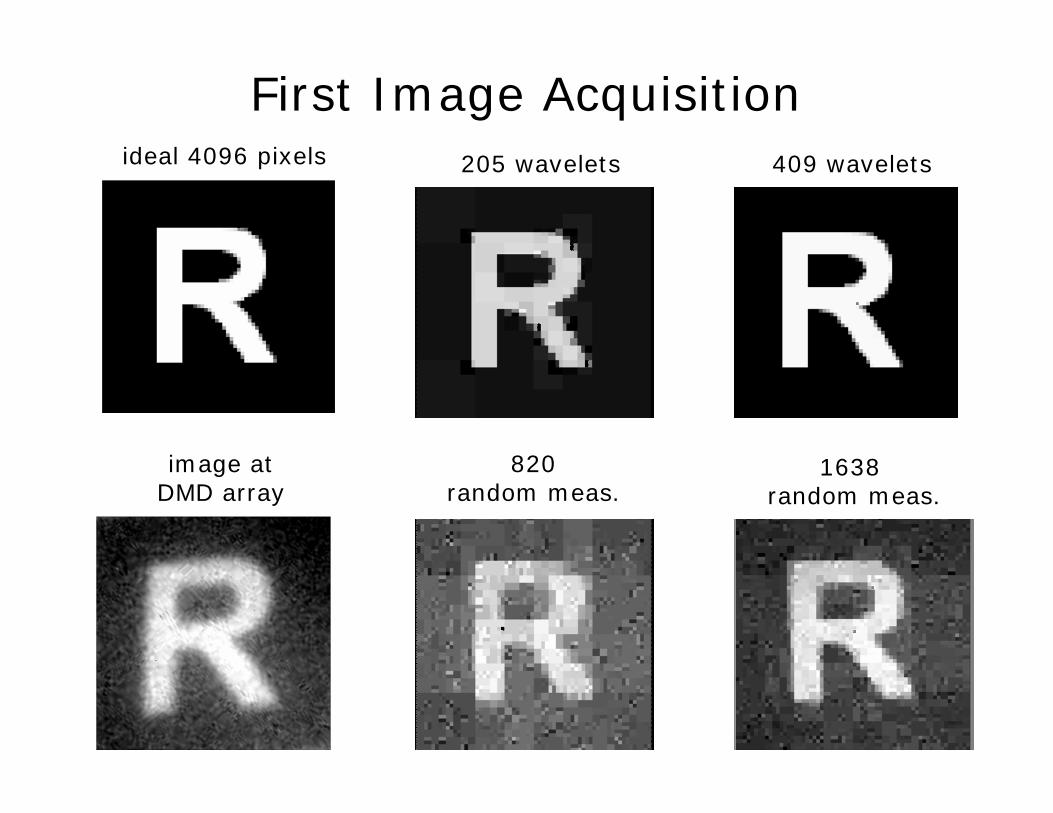
First Image Acquisitionideal 4096 pixels 205 wavelets 409 wavelets
image atDMD array
820random meas.
1638 random meas.
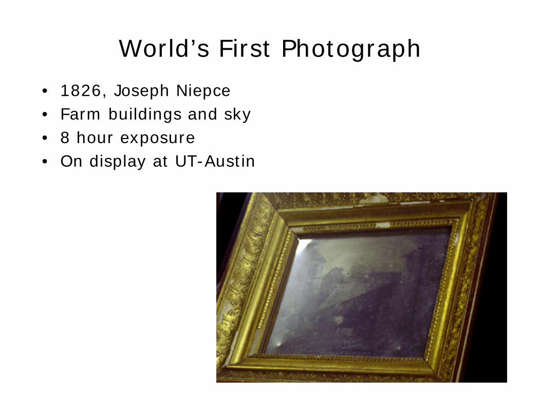
World’s First Photograph
• 1826, Joseph Niepce• Farm buildings and sky • 8 hour exposure• On display at UT-Austin
Conclusions
• Compressive sensing– exploit image sparsity information– based on new uncertainty principles– “sample smarter”, “universal hardware”– integrates sensing, compression, processing– matural when measurement is expensive
• Ongoing research– new kinds of cameras and imaging algorithms– new “analog-to-information” converters (analog CS)– new algs for distributed source coding
sensor nets, content distribution nets– fast algorithms– R/D analysis of CS (quantization)– CS vs. adaptive sampling
Contact Information
Richard BaraniukRice [email protected]/~richb
Robert NowakUniversity of [email protected]/~nowak
Justin RombergGeorgia Institute of [email protected]/~jrom
CS community websitedsp.rice.edu/cs