Embed Size (px)
Citation preview
Compressive Sensing and Structured RandomMatrices
Holger RauhutHausdorff Center for Mathematics
& Institute for Numerical SimulationUniversity of Bonn
Probability & Geometry in High DimensionsMarne la ValleeMay 19, 2010
Overview
• Compressive Sensing
• Random Sampling in Bounded Orthonormal Systems
• Partial Random Circulant Matrices
• Random Gabor Frames
Holger Rauhut, University of Bonn Structured Random Matrices 2
Key Ideas of compressive sensing
• Many types of signals, images are sparse, or can bewell-approximated by sparse ones.
• Question: Is it possible to recover such signals from only asmall number of (linear) measurements, i.e., withoutmeasuring all entries of the signal?
Holger Rauhut, University of Bonn Structured Random Matrices 3
Sparse Vectors in Finite Dimension
• coefficient vector: x ∈ CN , N ∈ N• support of x: supp x := {j , xj 6= 0}• s- sparse vectors: ‖x‖0 := |supp x| ≤ s.
s-term approximation error
σs(x)q := inf{‖x− z‖q, z is s-sparse}, 0 < q ≤ ∞.
x is called compressible if σs(x)q decays quickly in s.
Holger Rauhut, University of Bonn Structured Random Matrices 4
Compressed Sensing Problem
Reconstruct a s-sparse vector x ∈ CN (or a compressible vector)from its vector y of m measurements
y = Ax, A ∈ Cm×N .
Interesting case: s < m� N.
Underdetermined linear system of equations with a sparsityconstraint.
Preferably we would like to have a fast algorithm that performs thereconstruction.
Holger Rauhut, University of Bonn Structured Random Matrices 5
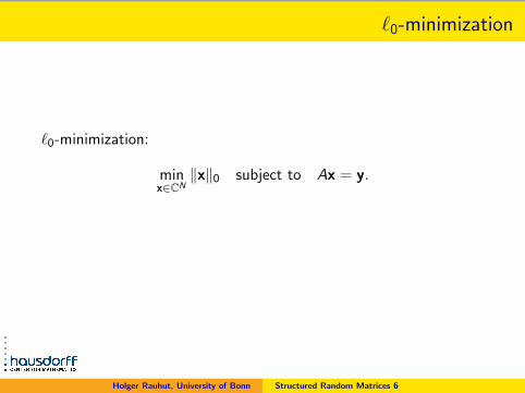
`0-minimization
`0-minimization:
minx∈CN
‖x‖0 subject to Ax = y.
Problem: `0-minimization is NP hard!
Holger Rauhut, University of Bonn Structured Random Matrices 6
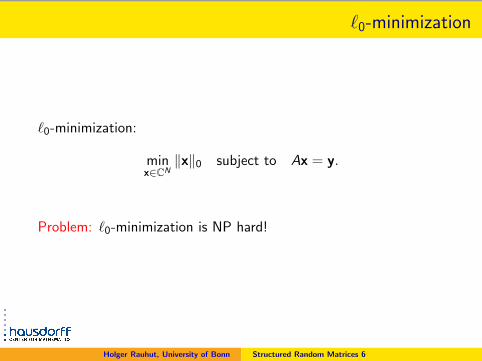
`0-minimization
`0-minimization:
minx∈CN
‖x‖0 subject to Ax = y.
Problem: `0-minimization is NP hard!
Holger Rauhut, University of Bonn Structured Random Matrices 6
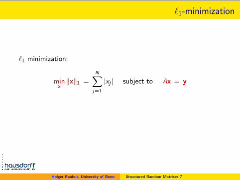
`1-minimization
`1 minimization:
minx‖x‖1 =
N∑j=1
|xj | subject to Ax = y
Convex relaxation of `0-minimization problem.
Efficient minimization methods available.
Holger Rauhut, University of Bonn Structured Random Matrices 7
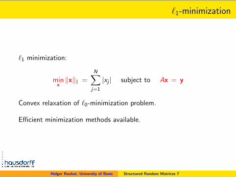
`1-minimization
`1 minimization:
minx‖x‖1 =
N∑j=1
|xj | subject to Ax = y
Convex relaxation of `0-minimization problem.
Efficient minimization methods available.
Holger Rauhut, University of Bonn Structured Random Matrices 7
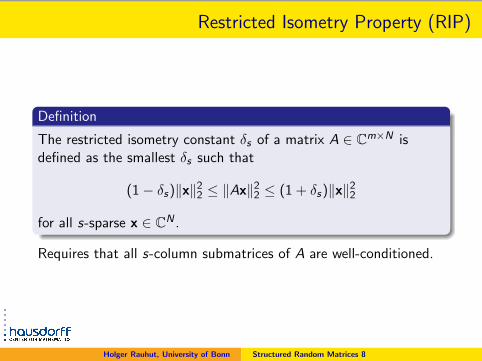
Restricted Isometry Property (RIP)
Definition
The restricted isometry constant δs of a matrix A ∈ Cm×N isdefined as the smallest δs such that
(1− δs)‖x‖22 ≤ ‖Ax‖2
2 ≤ (1 + δs)‖x‖22
for all s-sparse x ∈ CN .
Requires that all s-column submatrices of A are well-conditioned.
Holger Rauhut, University of Bonn Structured Random Matrices 8
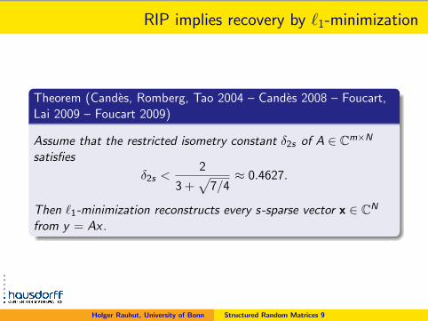
RIP implies recovery by `1-minimization
Theorem (Candes, Romberg, Tao 2004 – Candes 2008 – Foucart,Lai 2009 – Foucart 2009)
Assume that the restricted isometry constant δ2s of A ∈ Cm×N
satisfies
δ2s <2
3 +√
7/4≈ 0.4627.
Then `1-minimization reconstructs every s-sparse vector x ∈ CN
from y = Ax.
Holger Rauhut, University of Bonn Structured Random Matrices 9
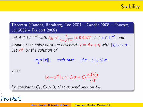
Stability
Theorem (Candes, Romberg, Tao 2004 – Candes 2008 – Foucart,Lai 2009 – Foucart 2009)
Let A ∈ Cm×N with δ2s <2
3+√
7/4≈ 0.4627. Let x ∈ CN , and
assume that noisy data are observed, y = Ax + η with ‖η‖2 ≤ σ.Let x# by the solution of
minz‖z‖1 such that ‖Az − y‖2 ≤ σ.
Then
‖x − x#‖2 ≤ C1σ + C2σs(x)1√
s
for constants C1,C2 > 0, that depend only on δ2s .
Holger Rauhut, University of Bonn Structured Random Matrices 10
Random Matrices
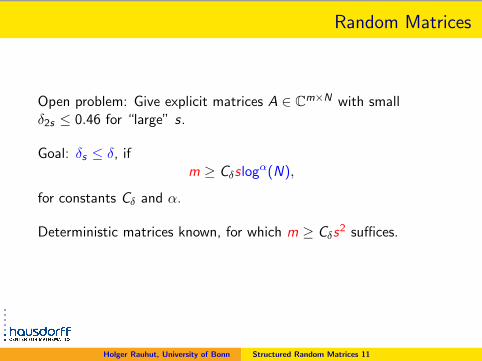
Open problem: Give explicit matrices A ∈ Cm×N with smallδ2s ≤ 0.46 for “large” s.
Goal: δs ≤ δ, ifm ≥ Cδs logα(N),
for constants Cδ and α.
Deterministic matrices known, for which m ≥ Cδs2 suffices.
Way out: consider random matrices.
Holger Rauhut, University of Bonn Structured Random Matrices 11
Random Matrices
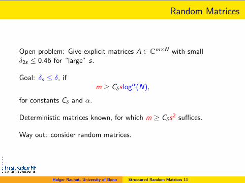
Open problem: Give explicit matrices A ∈ Cm×N with smallδ2s ≤ 0.46 for “large” s.
Goal: δs ≤ δ, ifm ≥ Cδs logα(N),
for constants Cδ and α.
Deterministic matrices known, for which m ≥ Cδs2 suffices.
Way out: consider random matrices.
Holger Rauhut, University of Bonn Structured Random Matrices 11
Random Matrices
Open problem: Give explicit matrices A ∈ Cm×N with smallδ2s ≤ 0.46 for “large” s.
Goal: δs ≤ δ, ifm ≥ Cδs logα(N),
for constants Cδ and α.
Deterministic matrices known, for which m ≥ Cδs2 suffices.
Way out: consider random matrices.
Holger Rauhut, University of Bonn Structured Random Matrices 11
RIP for Gaussian and Bernoulli matrices
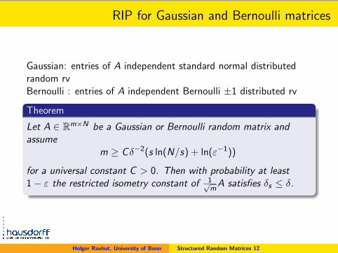
Gaussian: entries of A independent standard normal distributedrandom rvBernoulli : entries of A independent Bernoulli ±1 distributed rv
Theorem
Let A ∈ Rm×N be a Gaussian or Bernoulli random matrix andassume
m ≥ Cδ−2(s ln(N/s) + ln(ε−1))
for a universal constant C > 0. Then with probability at least1− ε the restricted isometry constant of 1√
mA satisfies δs ≤ δ.
Holger Rauhut, University of Bonn Structured Random Matrices 12
Consequence
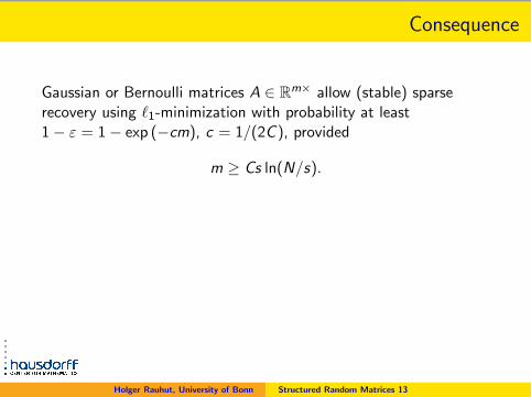
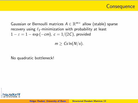
Gaussian or Bernoulli matrices A ∈ Rm× allow (stable) sparserecovery using `1-minimization with probability at least1− ε = 1− exp (−cm), c = 1/(2C ), provided
m ≥ Cs ln(N/s).
No quadratic bottleneck!
Bound is optimal as follows from bounds for Gelfand widths of`Np -balls (0 < p ≤ 1),Kashin (1977), Gluskin – Garnaev (1984), Carl – Pajor (1988),Vybiral (2008), Foucart – Pajor – Rauhut – Ullrich (2010).
Holger Rauhut, University of Bonn Structured Random Matrices 13
Consequence
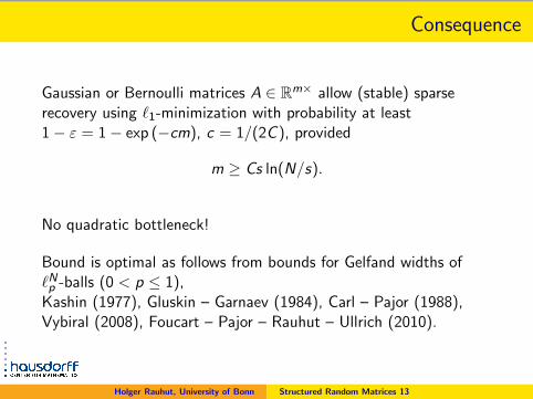
Gaussian or Bernoulli matrices A ∈ Rm× allow (stable) sparserecovery using `1-minimization with probability at least1− ε = 1− exp (−cm), c = 1/(2C ), provided
m ≥ Cs ln(N/s).
No quadratic bottleneck!
Bound is optimal as follows from bounds for Gelfand widths of`Np -balls (0 < p ≤ 1),Kashin (1977), Gluskin – Garnaev (1984), Carl – Pajor (1988),Vybiral (2008), Foucart – Pajor – Rauhut – Ullrich (2010).
Holger Rauhut, University of Bonn Structured Random Matrices 13
Structured Random Matrices
Why structure?
• Applications impose structure due to physical constraints,limited freedom to inject randomness.
• Fast matrix vector multiplies (FFT) in recovery algorithms,unstructured random matrices impracticable for large scaleapplications.
• Storage problems for unstructured matrices.
Holger Rauhut, University of Bonn Structured Random Matrices 14
Bounded orthonormal systems (BOS)
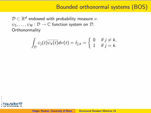
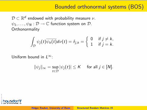
D ⊂ Rd endowed with probability measure ν.ψ1, . . . , ψN : D → C function system on D.
Orthonormality∫Dψj(t)ψk(t)dν(t) = δj ,k =
{0 if j 6= k,1 if j = k.
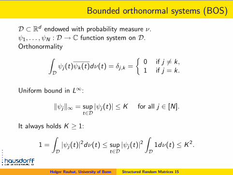
Uniform bound in L∞:
‖ψj‖∞ = supt∈D|ψj(t)| ≤ K for all j ∈ [N].
It always holds K ≥ 1:
1 =
∫D|ψj(t)|2dν(t) ≤ sup
t∈D|ψj(t)|2
∫D
1dν(t) ≤ K 2.
Holger Rauhut, University of Bonn Structured Random Matrices 15
Bounded orthonormal systems (BOS)
D ⊂ Rd endowed with probability measure ν.ψ1, . . . , ψN : D → C function system on D.Orthonormality∫
Dψj(t)ψk(t)dν(t) = δj ,k =
{0 if j 6= k,1 if j = k.
Uniform bound in L∞:
‖ψj‖∞ = supt∈D|ψj(t)| ≤ K for all j ∈ [N].
It always holds K ≥ 1:
1 =
∫D|ψj(t)|2dν(t) ≤ sup
t∈D|ψj(t)|2
∫D
1dν(t) ≤ K 2.
Holger Rauhut, University of Bonn Structured Random Matrices 15
Sampling
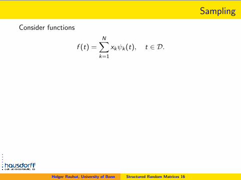
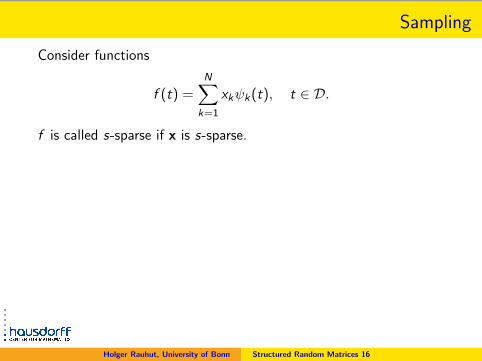
Consider functions
f (t) =N∑
k=1
xkψk(t), t ∈ D.
f is called s-sparse if x is s-sparse.Sampling points t1, . . . , tm ∈ D. Sample values:
y` = f (t`) =N∑
k=1
xkψk(t`) , ` ∈ [m].
Sampling matrix A ∈ Cm×N with entries
A`,k = ψk(t`), ` ∈ [m], k ∈ [N].
Theny = Ax.
Holger Rauhut, University of Bonn Structured Random Matrices 16
Sampling
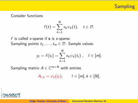
Consider functions
f (t) =N∑
k=1
xkψk(t), t ∈ D.
f is called s-sparse if x is s-sparse.
Sampling points t1, . . . , tm ∈ D. Sample values:
y` = f (t`) =N∑
k=1
xkψk(t`) , ` ∈ [m].
Sampling matrix A ∈ Cm×N with entries
A`,k = ψk(t`), ` ∈ [m], k ∈ [N].
Theny = Ax.
Holger Rauhut, University of Bonn Structured Random Matrices 16

Sampling
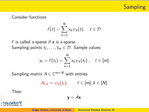
Consider functions
f (t) =N∑
k=1
xkψk(t), t ∈ D.
f is called s-sparse if x is s-sparse.Sampling points t1, . . . , tm ∈ D. Sample values:
y` = f (t`) =N∑
k=1
xkψk(t`) , ` ∈ [m].
Sampling matrix A ∈ Cm×N with entries
A`,k = ψk(t`), ` ∈ [m], k ∈ [N].
Theny = Ax.
Holger Rauhut, University of Bonn Structured Random Matrices 16
Sampling
Consider functions
f (t) =N∑
k=1
xkψk(t), t ∈ D.
f is called s-sparse if x is s-sparse.Sampling points t1, . . . , tm ∈ D. Sample values:
y` = f (t`) =N∑
k=1
xkψk(t`) , ` ∈ [m].
Sampling matrix A ∈ Cm×N with entries
A`,k = ψk(t`), ` ∈ [m], k ∈ [N].
Theny = Ax.
Holger Rauhut, University of Bonn Structured Random Matrices 16
Sparse Recovery
Problem: Reconstruct s-sparse f — equivalently x — from itssample values y = Ax.
We consider `1-minimization as recovery method.
Behavior of A as measurement matrix?
Holger Rauhut, University of Bonn Structured Random Matrices 17
Sparse Recovery
Problem: Reconstruct s-sparse f — equivalently x — from itssample values y = Ax.
We consider `1-minimization as recovery method.
Behavior of A as measurement matrix?
Holger Rauhut, University of Bonn Structured Random Matrices 17
Random Sampling
Choose sampling points t1, . . . , t` independently at randomaccording to the measure ν, that is,
P(t` ∈ B) = ν(B), for all measurable B ⊂ D.
The sampling matrix A is then a structured random matrix.
Holger Rauhut, University of Bonn Structured Random Matrices 18

Random Sampling
Choose sampling points t1, . . . , t` independently at randomaccording to the measure ν, that is,
P(t` ∈ B) = ν(B), for all measurable B ⊂ D.
The sampling matrix A is then a structured random matrix.
Holger Rauhut, University of Bonn Structured Random Matrices 18
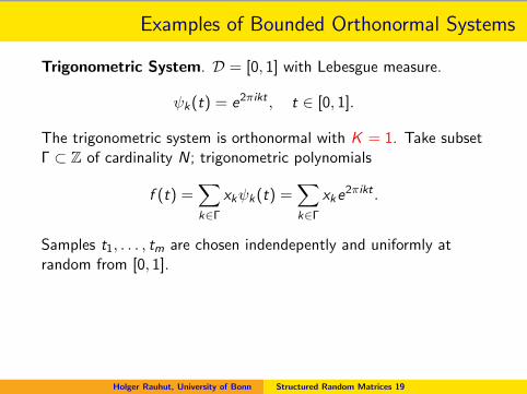
Examples of Bounded Orthonormal Systems
Trigonometric System. D = [0, 1] with Lebesgue measure.
ψk(t) = e2πikt , t ∈ [0, 1].
The trigonometric system is orthonormal with K = 1.
Take subsetΓ ⊂ Z of cardinality N; trigonometric polynomials
f (t) =∑k∈Γ
xkψk(t) =∑k∈Γ
xke2πikt .
Samples t1, . . . , tm are chosen indendepently and uniformly atrandom from [0, 1]. Nonequispaced random Fourier matrix
A`,k = e2πikt` , ` ∈ [m], k ∈ Γ.
Fast matrix vector multiply using the nonequispaced fast Fouriertransform (NFFT).
Holger Rauhut, University of Bonn Structured Random Matrices 19
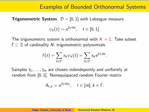
Examples of Bounded Orthonormal Systems
Trigonometric System. D = [0, 1] with Lebesgue measure.
ψk(t) = e2πikt , t ∈ [0, 1].
The trigonometric system is orthonormal with K = 1. Take subsetΓ ⊂ Z of cardinality N; trigonometric polynomials
f (t) =∑k∈Γ
xkψk(t) =∑k∈Γ
xke2πikt .
Samples t1, . . . , tm are chosen indendepently and uniformly atrandom from [0, 1]. Nonequispaced random Fourier matrix
A`,k = e2πikt` , ` ∈ [m], k ∈ Γ.
Fast matrix vector multiply using the nonequispaced fast Fouriertransform (NFFT).
Holger Rauhut, University of Bonn Structured Random Matrices 19
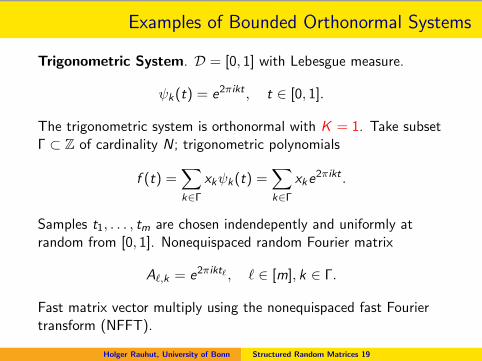
Examples of Bounded Orthonormal Systems
Trigonometric System. D = [0, 1] with Lebesgue measure.
ψk(t) = e2πikt , t ∈ [0, 1].
The trigonometric system is orthonormal with K = 1. Take subsetΓ ⊂ Z of cardinality N; trigonometric polynomials
f (t) =∑k∈Γ
xkψk(t) =∑k∈Γ
xke2πikt .
Samples t1, . . . , tm are chosen indendepently and uniformly atrandom from [0, 1].
Nonequispaced random Fourier matrix
A`,k = e2πikt` , ` ∈ [m], k ∈ Γ.
Fast matrix vector multiply using the nonequispaced fast Fouriertransform (NFFT).
Holger Rauhut, University of Bonn Structured Random Matrices 19
Examples of Bounded Orthonormal Systems
Trigonometric System. D = [0, 1] with Lebesgue measure.
ψk(t) = e2πikt , t ∈ [0, 1].
The trigonometric system is orthonormal with K = 1. Take subsetΓ ⊂ Z of cardinality N; trigonometric polynomials
f (t) =∑k∈Γ
xkψk(t) =∑k∈Γ
xke2πikt .
Samples t1, . . . , tm are chosen indendepently and uniformly atrandom from [0, 1]. Nonequispaced random Fourier matrix
A`,k = e2πikt` , ` ∈ [m], k ∈ Γ.
Fast matrix vector multiply using the nonequispaced fast Fouriertransform (NFFT).
Holger Rauhut, University of Bonn Structured Random Matrices 19
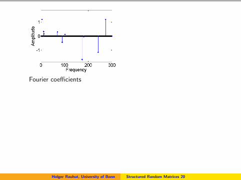
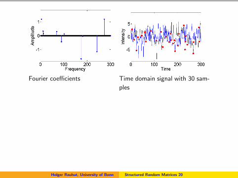
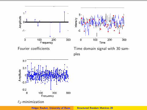
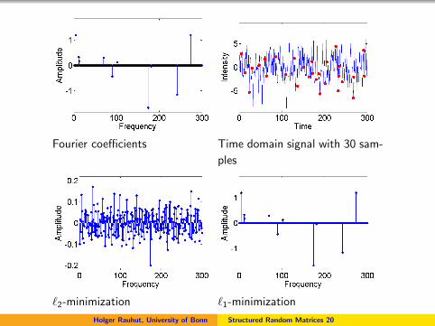
Fourier coefficients
Time domain signal with 30 sam-
ples
`2-minimization `1-minimization
Holger Rauhut, University of Bonn Structured Random Matrices 20
Fourier coefficients Time domain signal with 30 sam-
ples
`2-minimization `1-minimization
Holger Rauhut, University of Bonn Structured Random Matrices 20
Fourier coefficients Time domain signal with 30 sam-
ples
`2-minimization
`1-minimization
Holger Rauhut, University of Bonn Structured Random Matrices 20
Fourier coefficients Time domain signal with 30 sam-
ples
`2-minimization `1-minimization
Holger Rauhut, University of Bonn Structured Random Matrices 20
Further examples
• Real trigonometric polynomials
• Discrete systems – Random rows of bounded orthogonalmatrices
• Random partial Fourier matrices
• Legendre polynomials (needs a “twist”, see below)
Holger Rauhut, University of Bonn Structured Random Matrices 21
RIP estimate
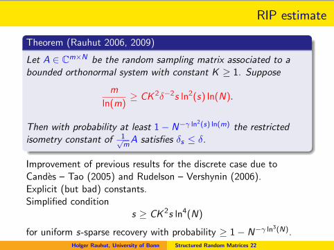
Theorem (Rauhut 2006, 2009)
Let A ∈ Cm×N be the random sampling matrix associated to abounded orthonormal system with constant K ≥ 1. Suppose
m
ln(m)≥ CK 2δ−2s ln2(s) ln(N).
Then with probability at least 1− N−γ ln2(s) ln(m) the restrictedisometry constant of 1√
mA satisfies δs ≤ δ.
Improvement of previous results for the discrete case due toCandes – Tao (2005) and Rudelson – Vershynin (2006).Explicit (but bad) constants.Simplified condition
s ≥ CK 2s ln4(N)
for uniform s-sparse recovery with probability ≥ 1− N−γ ln3(N).Holger Rauhut, University of Bonn Structured Random Matrices 22
Legendre Polynomials
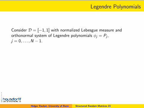
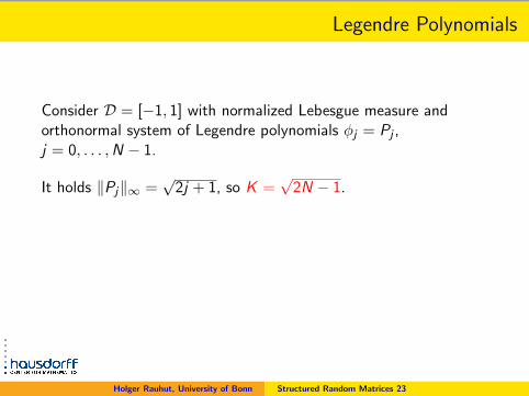
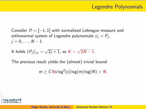
Consider D = [−1, 1] with normalized Lebesgue measure andorthonormal system of Legendre polynomials φj = Pj ,j = 0, . . . ,N − 1.
It holds ‖Pj‖∞ =√
2j + 1, so K =√
2N − 1.
The previous result yields the (almost) trivial bound
m ≥ C Ns log2(s) log(m) log(N) > N.
Can we do better?
Holger Rauhut, University of Bonn Structured Random Matrices 23
Legendre Polynomials
Consider D = [−1, 1] with normalized Lebesgue measure andorthonormal system of Legendre polynomials φj = Pj ,j = 0, . . . ,N − 1.
It holds ‖Pj‖∞ =√
2j + 1, so K =√
2N − 1.
The previous result yields the (almost) trivial bound
m ≥ C Ns log2(s) log(m) log(N) > N.
Can we do better?
Holger Rauhut, University of Bonn Structured Random Matrices 23
Random Chebyshev sampling
Do not sample uniformly, but with respect to the “Chebyshev”probability measure
ν(dx) =1
π(1− x2)−1/2dx on [−1, 1].
The functions
gj(x) =
√π
2(1− x2)1/4Pj(x)
are orthonormal with respect to ν.
A classical estimate for Legendre polynomials states that
supx∈[−1,1]
|gj(x)| ≤√
2 for all j ∈ N0.
Holger Rauhut, University of Bonn Structured Random Matrices 24
Random Chebyshev sampling
Do not sample uniformly, but with respect to the “Chebyshev”probability measure
ν(dx) =1
π(1− x2)−1/2dx on [−1, 1].
The functions
gj(x) =
√π
2(1− x2)1/4Pj(x)
are orthonormal with respect to ν.A classical estimate for Legendre polynomials states that
supx∈[−1,1]
|gj(x)| ≤√
2 for all j ∈ N0.
Holger Rauhut, University of Bonn Structured Random Matrices 24
Random sampling of sparse Legendre expansions
Theorem (Rauhut – Ward 2010)
Let Pj , j = 0, . . . ,N − 1, be the normalized Legendre polynomials,and let x`, ` = 1, . . . ,m, be sampling points in [−1, 1] which arechosen independently at random according to Chebyshevprobability measure π−1(1− x2)−1/2dx on [−1, 1]. Assume
m ≥ Cs log4(N).
Then with probability at least 1− N−γ log3(N) every s-sparseLegendre expansion
f (x) =N−1∑j=0
xjPj(x)
can be recovered from y = (f (x`))m`=1 via `1-minimization.
Holger Rauhut, University of Bonn Structured Random Matrices 25
Proof Idea
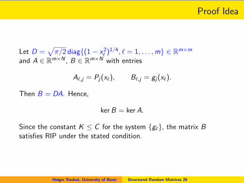
Let D =√π/2 diag{(1− x2
` )1/4, ` = 1, . . . ,m} ∈ Rm×m
and A ∈ Rm×N , B ∈ Rm×N with entries
A`,j = Pj(x`), B`,j = gj(x`).
Then B = DA. Hence,
ker B = ker A.
Since the constant K ≤ C for the system {g`}, the matrix Bsatisfies RIP under the stated condition.
Holger Rauhut, University of Bonn Structured Random Matrices 26

Circulant matrices
Circulant matrix: For b = (b0, b1, . . . , bN−1) ∈ CN letΦ = Φ(b) ∈ CN×N be the matrix with entries Φi ,j = bj−i mod N ,
Φ(b) =
b0 b1 · · · · · · bN−1
bN−1 b0 b1 · · · bN−2...
......
......
b1 b2 · · · bN−1 b0
.
Holger Rauhut, University of Bonn Structured Random Matrices 27
Partial random circulant matrices
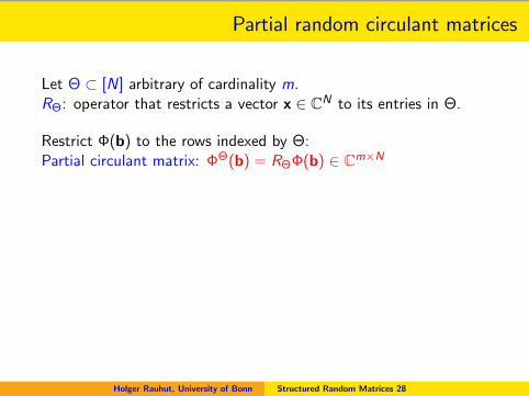
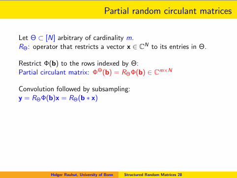
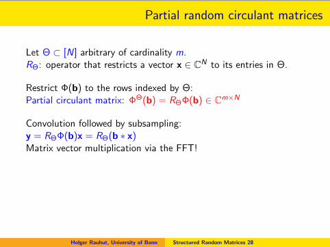
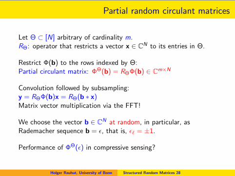
Let Θ ⊂ [N] arbitrary of cardinality m.RΘ: operator that restricts a vector x ∈ CN to its entries in Θ.
Restrict Φ(b) to the rows indexed by Θ:Partial circulant matrix: ΦΘ(b) = RΘΦ(b) ∈ Cm×N
Convolution followed by subsampling:y = RΘΦ(b)x = RΘ(b ∗ x)Matrix vector multiplication via the FFT!
We choose the vector b ∈ CN at random, in particular, asRademacher sequence b = ε, that is, ε` = ±1.
Performance of ΦΘ(ε) in compressive sensing?
Holger Rauhut, University of Bonn Structured Random Matrices 28
Partial random circulant matrices
Let Θ ⊂ [N] arbitrary of cardinality m.RΘ: operator that restricts a vector x ∈ CN to its entries in Θ.
Restrict Φ(b) to the rows indexed by Θ:Partial circulant matrix: ΦΘ(b) = RΘΦ(b) ∈ Cm×N
Convolution followed by subsampling:y = RΘΦ(b)x = RΘ(b ∗ x)
Matrix vector multiplication via the FFT!
We choose the vector b ∈ CN at random, in particular, asRademacher sequence b = ε, that is, ε` = ±1.
Performance of ΦΘ(ε) in compressive sensing?
Holger Rauhut, University of Bonn Structured Random Matrices 28
Partial random circulant matrices
Let Θ ⊂ [N] arbitrary of cardinality m.RΘ: operator that restricts a vector x ∈ CN to its entries in Θ.
Restrict Φ(b) to the rows indexed by Θ:Partial circulant matrix: ΦΘ(b) = RΘΦ(b) ∈ Cm×N
Convolution followed by subsampling:y = RΘΦ(b)x = RΘ(b ∗ x)Matrix vector multiplication via the FFT!
We choose the vector b ∈ CN at random, in particular, asRademacher sequence b = ε, that is, ε` = ±1.
Performance of ΦΘ(ε) in compressive sensing?
Holger Rauhut, University of Bonn Structured Random Matrices 28
Partial random circulant matrices
Let Θ ⊂ [N] arbitrary of cardinality m.RΘ: operator that restricts a vector x ∈ CN to its entries in Θ.
Restrict Φ(b) to the rows indexed by Θ:Partial circulant matrix: ΦΘ(b) = RΘΦ(b) ∈ Cm×N
Convolution followed by subsampling:y = RΘΦ(b)x = RΘ(b ∗ x)Matrix vector multiplication via the FFT!
We choose the vector b ∈ CN at random, in particular, asRademacher sequence b = ε, that is, ε` = ±1.
Performance of ΦΘ(ε) in compressive sensing?
Holger Rauhut, University of Bonn Structured Random Matrices 28
Nonuniform recovery result for circulant matrices
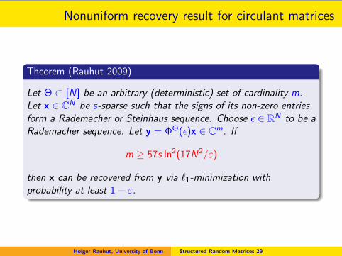
Theorem (Rauhut 2009)
Let Θ ⊂ [N] be an arbitrary (deterministic) set of cardinality m.Let x ∈ CN be s-sparse such that the signs of its non-zero entriesform a Rademacher or Steinhaus sequence. Choose ε ∈ RN to be aRademacher sequence. Let y = ΦΘ(ε)x ∈ Cm. If
m ≥ 57s ln2(17N2/ε)
then x can be recovered from y via `1-minimization withprobability at least 1− ε.
Holger Rauhut, University of Bonn Structured Random Matrices 29
RIP estimate for partial circulant matrices
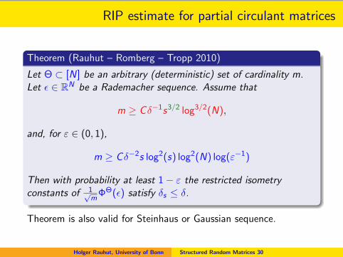
Theorem (Rauhut – Romberg – Tropp 2010)
Let Θ ⊂ [N] be an arbitrary (deterministic) set of cardinality m.Let ε ∈ RN be a Rademacher sequence. Assume that
m ≥ Cδ−1s3/2 log3/2(N),
and, for ε ∈ (0, 1),
m ≥ Cδ−2s log2(s) log2(N) log(ε−1)
Then with probability at least 1− ε the restricted isometryconstants of 1√
mΦΘ(ε) satisfy δs ≤ δ.
Theorem is also valid for Steinhaus or Gaussian sequence.
Holger Rauhut, University of Bonn Structured Random Matrices 30

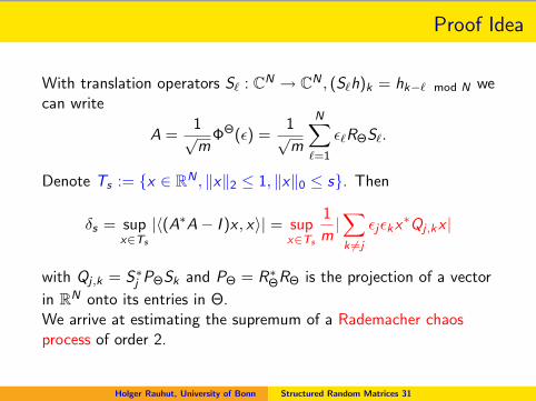
Proof Idea
With translation operators S` : CN → CN , (S`h)k = hk−` mod N wecan write
A =1√m
ΦΘ(ε) =1√m
N∑`=1
ε`RΘS`.
Denote Ts := {x ∈ RN , ‖x‖2 ≤ 1, ‖x‖0 ≤ s}. Then
δs = supx∈Ts
|〈(A∗A− I )x , x〉| = supx∈Ts
1
m|∑k 6=j
εjεkx∗Qj ,kx |
with Qj ,k = S∗j PΘSk and PΘ = R∗ΘRΘ is the projection of a vector
in RN onto its entries in Θ.We arrive at estimating the supremum of a Rademacher chaosprocess of order 2.
Holger Rauhut, University of Bonn Structured Random Matrices 31

Dudley type inequality for chaos processes
Theorem (Talagrand)
Let Yx =∑
k,j εj εkZjk(x) be a scalar Rademacher chaos processindexed by x ∈ T , with Zjj(x) = 0 and Zjk(x) = Zkj(x). Introducetwo metrics on T , with (Z (x))j ,k = Zjk(x)j ,k ,
d1(x , y) = ‖Z (x)− Z (y)‖F ,d2(x , y) = ‖Z (x)− Z (y)‖2→2.
Let N(T , di , u) denote the minimal number of balls of radius u inthe metric di necessary to cover T . There exists a universalconstant K such that, for an arbitrary x0 ∈ T ,
E supx∈T|Yx − Yx0 | ≤
K max
{∫ ∞0
√log(N(T , d1, u))du,
∫ ∞0
log(N(T , d2, u))du
}.
Holger Rauhut, University of Bonn Structured Random Matrices 32
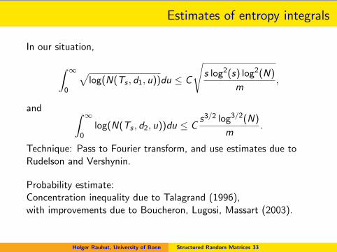
Estimates of entropy integrals
In our situation,
∫ ∞0
√log(N(Ts , d1, u))du ≤ C
√s log2(s) log2(N)
m,
and ∫ ∞0
log(N(Ts , d2, u))du ≤ Cs3/2 log3/2(N)
m.
Technique: Pass to Fourier transform, and use estimates due toRudelson and Vershynin.
Probability estimate:Concentration inequality due to Talagrand (1996),with improvements due to Boucheron, Lugosi, Massart (2003).
Holger Rauhut, University of Bonn Structured Random Matrices 33
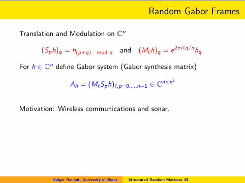
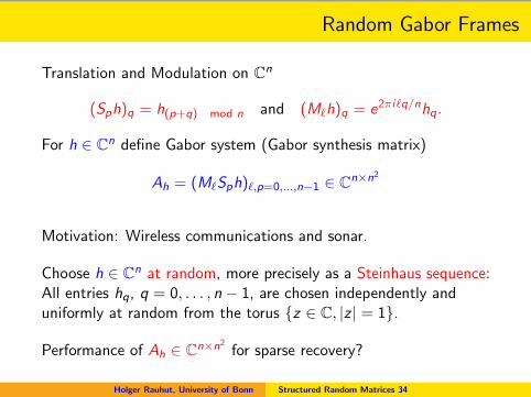
Random Gabor Frames
Translation and Modulation on Cn
(Sph)q = h(p+q) mod n and (M`h)q = e2πi`q/nhq.
For h ∈ Cn define Gabor system (Gabor synthesis matrix)
Ah = (M`Sph)`,p=0,...,n−1 ∈ Cn×n2
Motivation: Wireless communications and sonar.
Choose h ∈ Cn at random, more precisely as a Steinhaus sequence:All entries hq, q = 0, . . . , n − 1, are chosen independently anduniformly at random from the torus {z ∈ C, |z | = 1}.
Performance of Ah ∈ Cn×n2for sparse recovery?
Holger Rauhut, University of Bonn Structured Random Matrices 34
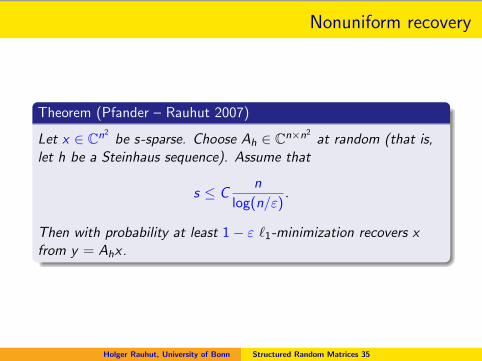
Nonuniform recovery
Theorem (Pfander – Rauhut 2007)
Let x ∈ Cn2be s-sparse. Choose Ah ∈ Cn×n2
at random (that is,let h be a Steinhaus sequence). Assume that
s ≤ Cn
log(n/ε).
Then with probability at least 1− ε `1-minimization recovers xfrom y = Ahx.
Holger Rauhut, University of Bonn Structured Random Matrices 35
RIP estimate
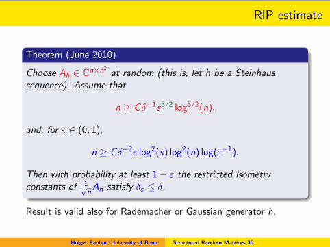
Theorem (June 2010)
Choose Ah ∈ Cn×n2at random (this is, let h be a Steinhaus
sequence). Assume that
n ≥ Cδ−1s3/2 log3/2(n),
and, for ε ∈ (0, 1),
n ≥ Cδ−2s log2(s) log2(n) log(ε−1).
Then with probability at least 1− ε the restricted isometryconstants of 1√
nAh satisfy δs ≤ δ.
Result is valid also for Rademacher or Gaussian generator h.
Holger Rauhut, University of Bonn Structured Random Matrices 36

THAT’S ALL
THANKS!
Holger Rauhut, University of Bonn Structured Random Matrices 37


![Compressive Structured Light for Recovering Inhomogeneous ... · Structured light has a long history in the computer vision community [Salvi et al., 2004]. It has matured into a robust](https://img.pdfslide.us/doc/110x75/5f9adf57156b4b62ed3955d9/compressive-structured-light-for-recovering-inhomogeneous-structured-light-has.jpg)