COMPRESSIVE CREEP OF A LIGHTWEIGHT, HIGH STRENGTH CONCRETE

COMPRESSIVE CREEP OF A LIGHTWEIGHT,

HIGH STRENGTH CONCRETE MIXTURE

by

Edward C. Vincent

Thesis presented to the faculty of the

Virginia Polytechnic Institute and State University

In partial fulfillment of the requirements for the degree of

Master of Science

in

Civil Engineering

Committee:

Richard E. Weyers, Chair

Thomas E. Cousins

Carin L. Roberts-Wollmann

January 10, 2003

Blacksburg, VA

Keywords: compressive creep, prediction models, shrinkage, lightweight aggregate

Copyright 2003, Edward C. Vincent

COMPRESSIVE CREEP OF A LIGHTWEIGHT,

HIGH STRENGTH CONCRETE MIXTURE

by

Edward C. Vincent

ABSTRACT Concrete undergoes volumetric changes throughout its service life. These changes are a result of

applied loads and shrinkage. Applied loads result in an instantaneous recoverable elastic

deformation and a slow, time dependent, inelastic deformation called creep. Creep without

moisture loss is referred to as basic creep and with moisture loss is referred to as drying creep.

Shrinkage is the combination of autogeneous, drying, and carbonation shrinkage. The

combination of creep, shrinkage, and elastic deformation is referred to as total strain.

The prestressed concrete beams in the Chickahominy River Bridge have been fabricated with a

lightweight, high strength concrete mixture (LTHSC). Laboratory test specimens have been cast

using the concrete materials and mixture proportions used in the fabrication of the bridge beams.

Two standard cure and two match cure batches have been loaded for 329 and 251 days,

respectively.

Prestress losses are generally calculated with the total strain predicted by the American Concrete

Institute Committee 209 recommendations, ACI 209, or the European design code, CEB Model

Code 90. Two additional models that have been proposed are the B3 model by Bazant and

Baweja, and the GL2000 model proposed by Gardner and Lockman. The four models are

analyzed to determine the most precise model for the LTHSC mixture. Only ACI 209

considered lightweight aggregates during model development. GL2000 considers aggregate

stiffness in the model.

ACI 209 was the best predictor of total strain and individual time dependent deformations for the

accelerated cure specimens. CEB Mode Code 90 was the best predictor of total strain for the

standard cure specimens. The best overall predictor of time dependent deformations was the

GL2000 model for the standard cure specimens.

iii

ACKNOWLEDGEMENTS

First, I would like to express my gratitude to Dr. Richard E. Weyers for his guidance and

assistance throughout this project. I also greatly appreciate the guidance of Dr. Thomas Cousins

and Dr. Carin Roberts-Wollmann as members of my research committee.

I would like to thank the Virginia Transportation Research Council for providing the funding for

this project.

I am grateful for the many people that contributed to this project. I owe a great deal of gratitude

to David Mokarem for his help in getting this project underway. I am also grateful to Richard

Meyerson for his work involving a previous creep study. In addition, I would like to thank

technicians, Brett Farmer and Denis Huffman for their insight and technical expertise.

My appreciation goes out to the faculty of the Structural Engineering and Materials Program for

the valuable learning experiences and leading me realize that a glass of water is not really half

full or half empty, but has a safety factor of two. I also would like to thank Dr. Anderson-Cook

in the Statistics Department for the valuable learning experiences.

Most importantly, I would like to thank my mother, Catherine Ritchey. I cannot give enough

credit for her love and support. I also would like to thank my grandparents, Frank and Opal, my

sister, Valerie, and my stepfather, Tom, for their love and support.

I would like to thank my friends Michael Brown, Patricia Buchanan, James Fazio Jr., Allison

Haden, Brian McCormick, David Mokarem, Matthew Rowe, Kevin Siegel, and Megan Wheeler

for their support and friendship throughout the years.

iv

TABLE OF CONTENTS

ABSTRACT ................................................................................................................................................................ ii

ACKNOWLEDGEMENTS ...................................................................................................................................... iii

TABLE OF CONTENTS ...........................................................................................................................................iv

LIST OF FIGURES.................................................................................................................................................. vii

LIST OF TABLES......................................................................................................................................................ix

CHAPTER 1: INTRODUCTION...............................................................................................................................1

CHAPTER 2: PURPOSE AND SCOPE....................................................................................................................2

CHAPTER 3: METHODS AND MATERIALS .......................................................................................................3

3.1 INTRODUCTION ....................................................................................................................................................3 3.2 AGGREGATE PROPERTIES.....................................................................................................................................5 3.3 CEMENT PROPERTIES ...........................................................................................................................................5 3.4 CHEMICAL ADMIXTURES .....................................................................................................................................6 3.5 CREEP TESTING....................................................................................................................................................6 3.6 SHRINKAGE TESTING ...........................................................................................................................................8 3.7 STRENGTH AND MODULUS TESTING ....................................................................................................................8 3.8 THERMAL COEFFICIENT .......................................................................................................................................9

CHAPTER 4: RESULTS ..........................................................................................................................................10

4.1 INTRODUCTION ..................................................................................................................................................10 4.2 COMPRESSIVE STRENGTH ..................................................................................................................................11 4.3 TENSILE STRENGTH ...........................................................................................................................................13 4.4 MODULUS OF ELASTICITY..................................................................................................................................14 4.5 THERMAL COEFFICIENT .....................................................................................................................................16 4.6 EXPERIMENTAL AND PREDICTED STRAINS.........................................................................................................16 4.7 PREDICTION MODEL RESIDUALS........................................................................................................................24 4.8 SHRINKAGE PRISMS ...........................................................................................................................................37

CHAPTER 5: DISCUSSION AND ANALYSIS .....................................................................................................39

5.1 INTRODUCTION ..................................................................................................................................................39 5.2 COMPRESSIVE STRENGTH ..................................................................................................................................39 5.3 TENSILE STRENGTH ...........................................................................................................................................40 5.4 MODULUS OF ELASTICITY..................................................................................................................................41 5.5 THERMAL COEFFICIENT .....................................................................................................................................41 5.6 EXPERIMENTAL AND PREDICTED STRAINS.........................................................................................................42 5.7 EXPERIMENTAL STRAIN RELATIONSHIPS ...........................................................................................................43 5.8 EXPERIMENTAL PRECISION................................................................................................................................46 5.9 PREDICTION MODEL RESIDUALS........................................................................................................................49 5.10 RESIDUALS SQUARED ANALYSIS .....................................................................................................................52 5.11 PREDICTION MODEL RANKINGS.......................................................................................................................62 5.12 GL2000 STANDARD CURE SENSITIVITY ..........................................................................................................64

CHAPTER 6: CONCLUSIONS AND RECOMMENDATIONS ..........................................................................68

v

REFERENCES.......................................................................................................................................................... 71

APPENDIX A............................................................................................................................................................ 72

LITERATURE REVIEW AND PREDICTION MODELS ................................................................................................... 72 APPENDIX B .......................................................................................................................................................... 112

MIXING AND CURING DATA.................................................................................................................................. 112 APPENDIX C.......................................................................................................................................................... 121

PHOTOGRAPHS ...................................................................................................................................................... 121 APPENDIX D.......................................................................................................................................................... 124

CREEP FRAME CALIBRATION ................................................................................................................................ 124 APPENDIX E .......................................................................................................................................................... 128

ACCELERATED CURING......................................................................................................................................... 128 APPENDIX F .......................................................................................................................................................... 130

STRAIN MEASUREMENTS ...................................................................................................................................... 130 APPENDIX G.......................................................................................................................................................... 135

PERCENT SHRINKAGE MEASUREMENTS ................................................................................................................ 135 VITA ........................................................................................................................................................................ 137

vi

LIST OF FIGURES

Figure 1 Standard Cure Compressive Strengths ......................................................................................................... 11

Figure 2 Accelerated Cure Compressive Strengths..................................................................................................... 12

Figure 3 Tensile Strength............................................................................................................................................ 13

Figure 4 Standard Cure Modulus of Elasticity............................................................................................................ 14

Figure 5 Accelerated Cure Modulus of Elasticity ....................................................................................................... 15

Figure 6 Standard Cure Batch 2: Total, Creep, and Shrinkage Strain (6 by 12 in. cylinders)..................................... 18

Figure 7 Standard Cure Batch 3: Total, Creep, and Shrinkage Strain (6 by 12 in. cylinders)..................................... 18

Figure 8 Accelerated Cure Batch 4: Total, Creep, and Shrinkage Strain (4 by 8 in. cylinders).................................. 19

Figure 9 Accelerated Cure Batch 5: Total, Creep, and Shrinkage Strain (4 by 8 in. cylinders).................................. 19

Figure.10 ACI 209 Standard Cure .............................................................................................................................. 20

Figure 11 CEB 90 Standard Cure................................................................................................................................ 20

Figure 12 B3 Standard Cure........................................................................................................................................ 21

Figure 13 GL2000 Standard Cure ............................................................................................................................... 21

Figure 14 ACI 209 Accelerated Cure.......................................................................................................................... 22

Figure 15 CEB 90 Accelerated Cure........................................................................................................................... 22

Figure 16 B3 Accelerated Cure................................................................................................................................... 23

Figure 17 GL2000 Accelerated Cure .......................................................................................................................... 23

Figure 18 ACI 209 and Standard Cure Total Strain Residuals ................................................................................... 25

Figure 19 CEB 90 and Standard Cure Total Strain Residuals..................................................................................... 25

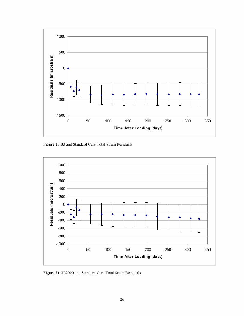
Figure 20 B3 and Standard Cure Total Strain Residuals............................................................................................. 26

Figure 21 GL2000 and Standard Cure Total Strain Residuals .................................................................................... 26

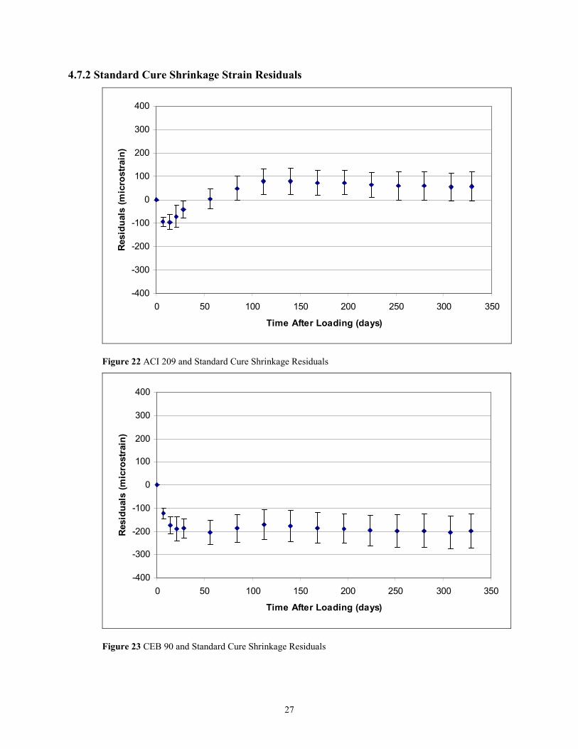
Figure 22 ACI 209 and Standard Cure Shrinkage Residuals ...................................................................................... 27

Figure 23 CEB 90 and Standard Cure Shrinkage Residuals ....................................................................................... 27

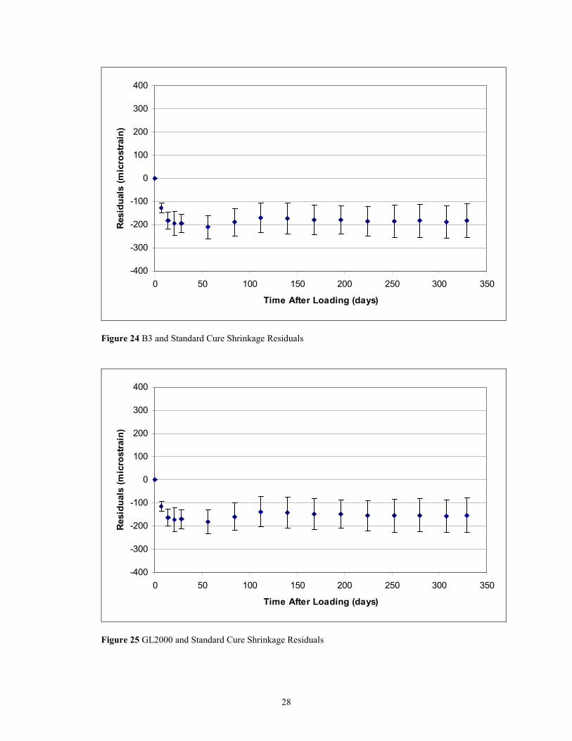
Figure 24 B3 and Standard Cure Shrinkage Residuals ............................................................................................... 28

Figure 25 GL2000 and Standard Cure Shrinkage Residuals....................................................................................... 28

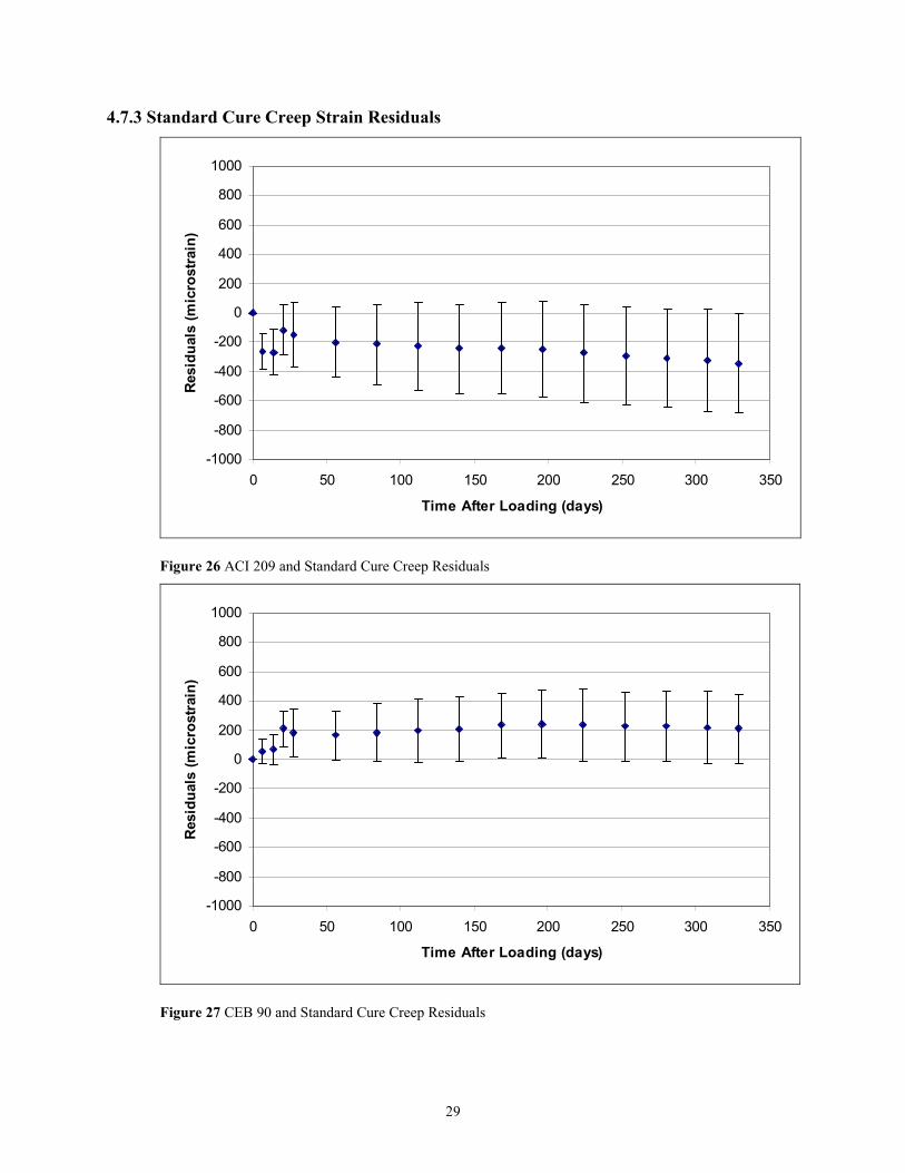
Figure 26 ACI 209 and Standard Cure Creep Residuals............................................................................................. 29

Figure 27 CEB 90 and Standard Cure Creep Residuals .............................................................................................. 29

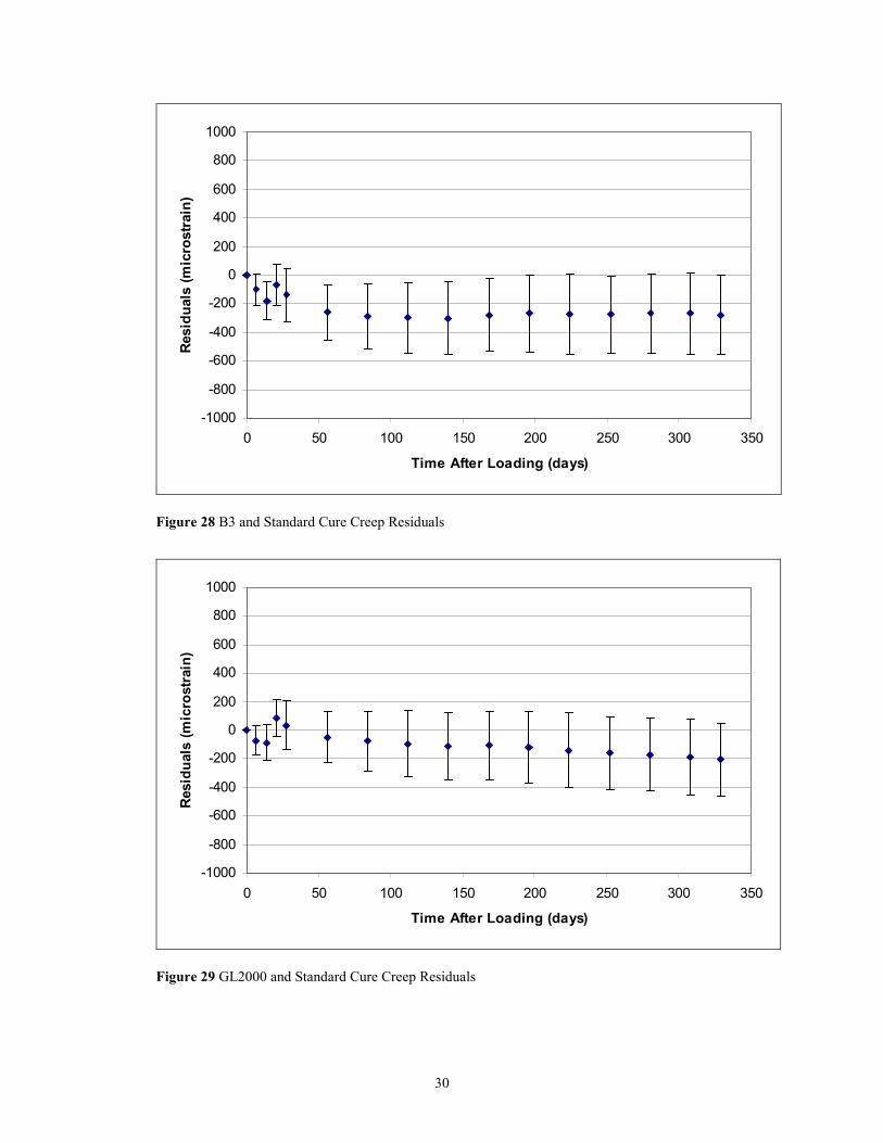
Figure 28 B3 and Standard Cure Creep Residuals ...................................................................................................... 30

Figure 29 GL2000 and Standard Cure Creep Residuals ............................................................................................. 30

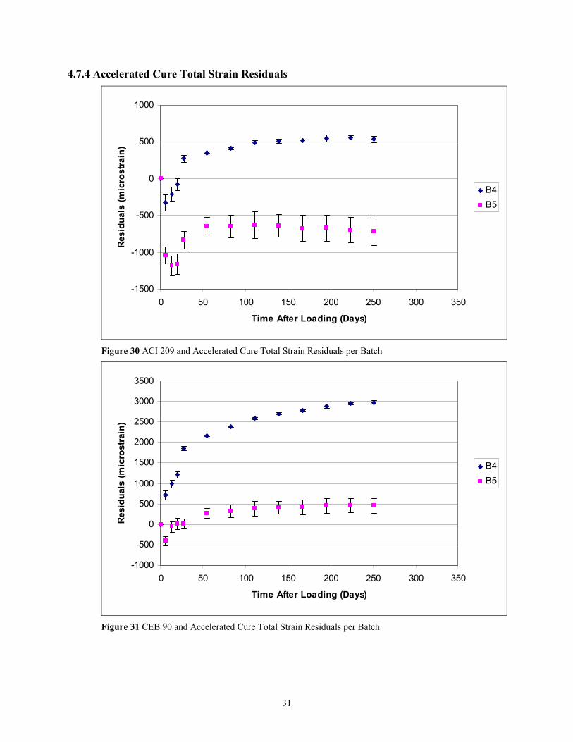
Figure 30 ACI 209 and Accelerated Cure Total Strain Residuals per Batch .............................................................. 31

Figure 31 CEB 90 and Accelerated Cure Total Strain Residuals per Batch ............................................................... 31

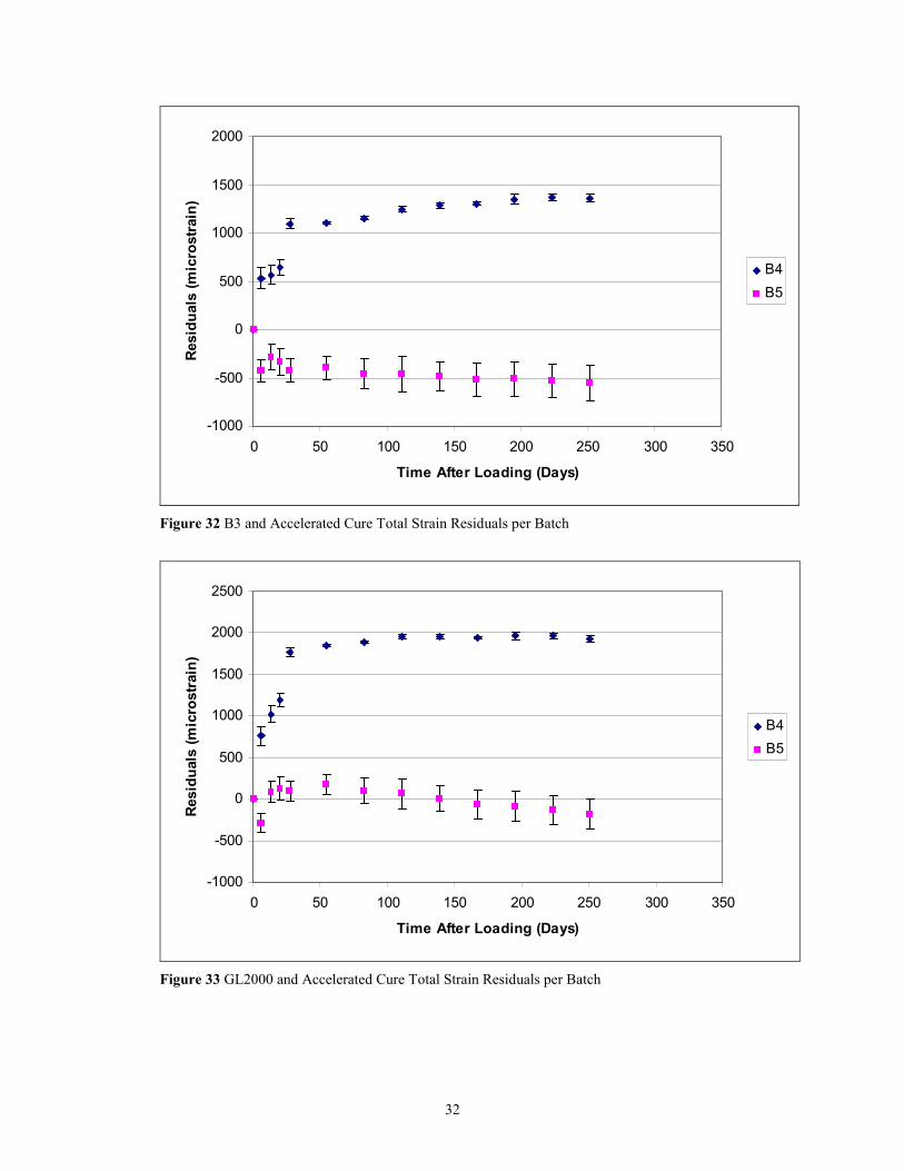
Figure 32 B3 and Accelerated Cure Total Strain Residuals per Batch ....................................................................... 32

Figure 33 GL2000 and Accelerated Cure Total Strain Residuals per Batch............................................................... 32

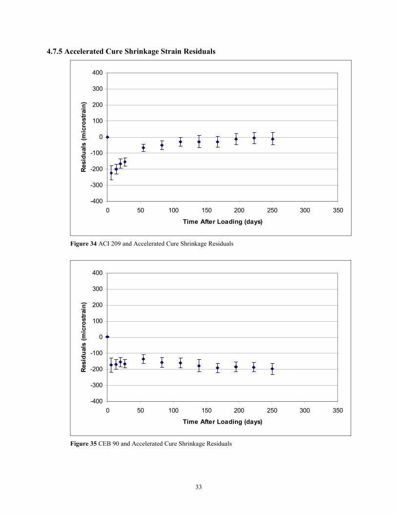
Figure 34 ACI 209 and Accelerated Cure Shrinkage Residuals ................................................................................. 33

vii

Figure 35 CEB 90 and Accelerated Cure Shrinkage Residuals .................................................................................. 33

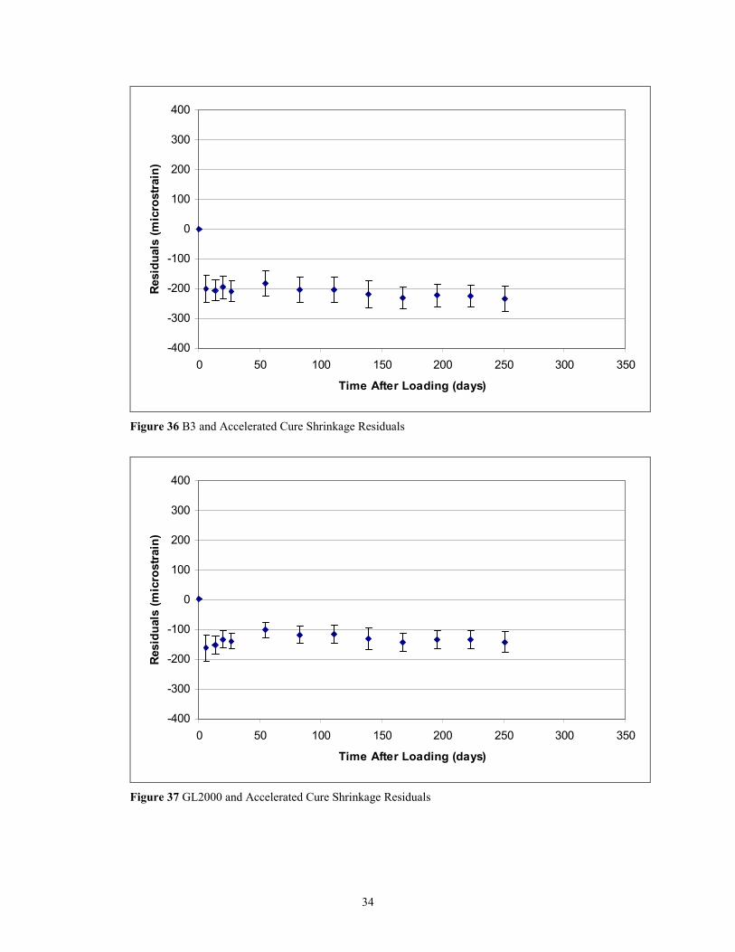
Figure 36 B3 and Accelerated Cure Shrinkage Residuals .......................................................................................... 34

Figure 37 GL2000 and Accelerated Cure Shrinkage Residuals.................................................................................. 34

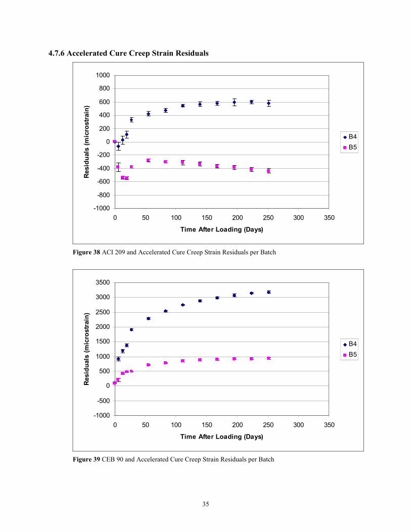
Figure 38 ACI 209 and Accelerated Cure Creep Strain Residuals per Batch ............................................................. 35

Figure 39 CEB 90 and Accelerated Cure Creep Strain Residuals per Batch .............................................................. 35

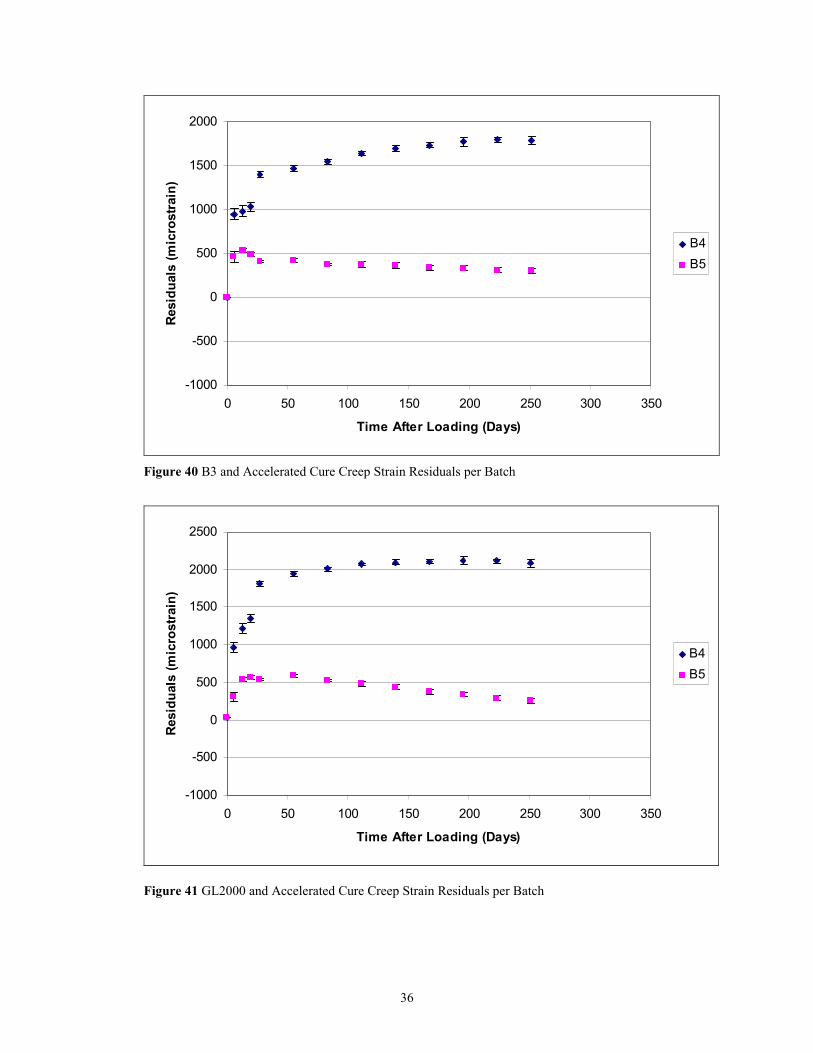
Figure 40 B3 and Accelerated Cure Creep Strain Residuals per Batch ...................................................................... 36

Figure 41 GL2000 and Accelerated Cure Creep Strain Residuals per Batch.............................................................. 36

Figure 42 Prism Data with ACI 209 and CEB 90 Models .......................................................................................... 38

Figure 43 Prism Data with B3 and GL2000 Models................................................................................................... 38

Figure 44 Average Total Strain: Size and Curing Relationship (microstrain). ........................................................... 44

Figure 45 Average Creep Strain: Size and Curing Relationship (microstrain) ........................................................... 44

Figure 46 Average Shrinkage Strain: Size and Curing Relationship (microstrain)..................................................... 45

Figure 47 Standard Cure Shrinkage Specimens: Volume to Surface Area Relationship ............................................ 45

Figure 48 Standard Cure Total Strain Residuals Squared ........................................................................................... 54

Figure 49 Standard Cure Shrinkage Residuals Squared.............................................................................................. 55

Figure 50 Standard Cure Creep Strain Residuals Squared.......................................................................................... 56

Figure 51 Accelerated Cure Total Strain Residuals Squared ...................................................................................... 58

Figure 52 Accelerated Cure Shrinkage Residuals Squared......................................................................................... 59

Figure 53 Accelerated Cure Creep Strain Residuals Squared ..................................................................................... 60

Figure 54 Residuals Squared for Shrinkage Prisms and the Prediction Models ......................................................... 61

Figure 55 Standard Cure Shrinkage Strain Sensitivity Analysis of the GL2000 K factor. ......................................... 65

Figure 56 Total Strain Sensitivity Analysis of the GL2000 K factor, Standard Cure. ................................................ 66

Figure 57 Accelerated Cure Shrinkage Strain Sensitivity Analysis of the GL2000 K factor...................................... 66

Figure 58 GL2000 K factor sensitivity with shrinkage prisms ................................................................................... 67

Figure 59 Batch 4 Maturity Curve Extremes and Bridge Beam Internal Curing Temperatures. .............................. 116

Figure 60 Batch 5 Maturity Curve Extremes and Bridge Beam Internal Curing Temperatures. .............................. 116

Figure 61 Creep Room Photograph........................................................................................................................... 122

Figure 62 The Sure Cure Accelerated Curing System Photograph........................................................................... 122

Figure 63 Whittemore Gage Photograph .................................................................................................................. 123

Figure 64 Side View Photograph of the Whittemore Gage....................................................................................... 123

Figure 65 Frame 1: Gage Pressure verse Applied Load............................................................................................ 126




viii

LIST OF TABLES

Table 1 LTHSC Test Matrix ......................................................................................................................................... 3

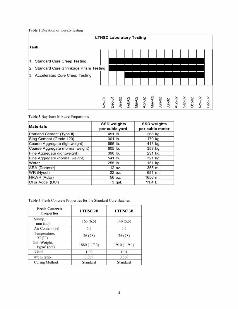
Table 2 Duration of weekly testing............................................................................................................................... 4

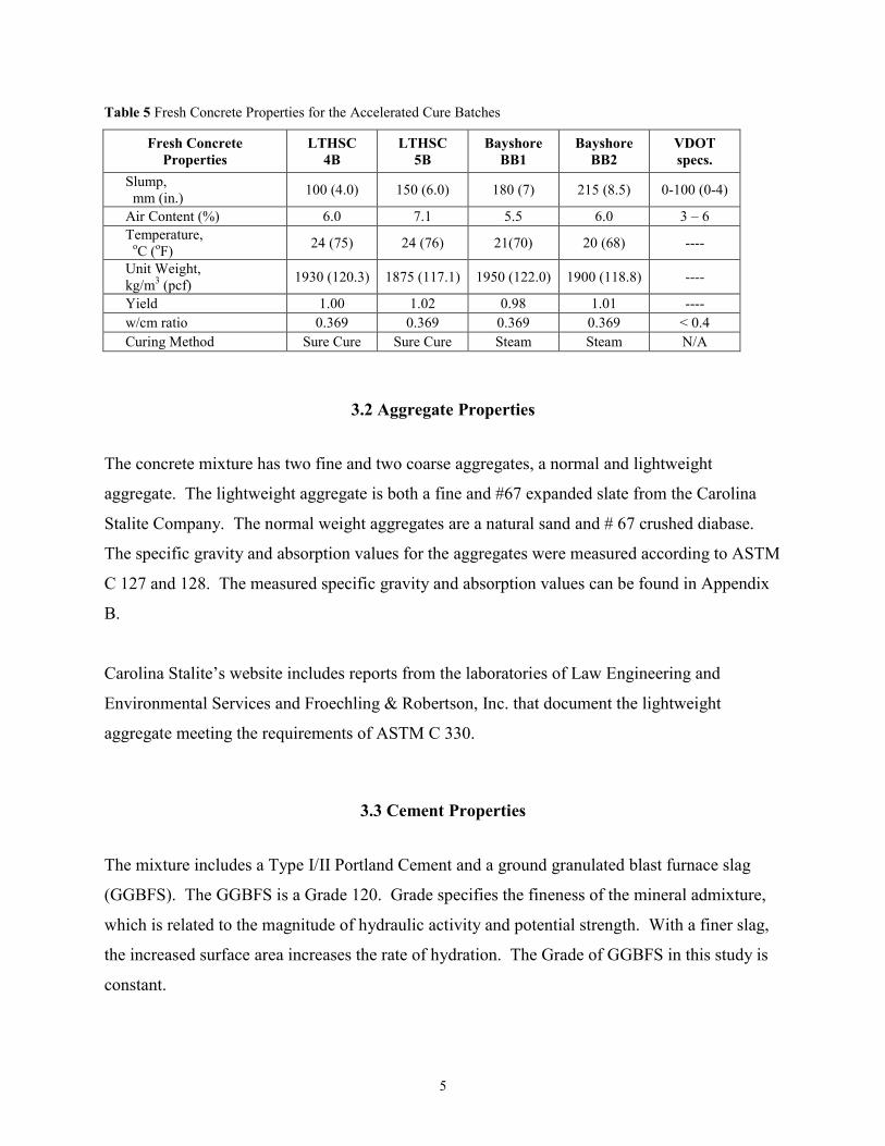
Table 3 Bayshore Mixture Proportions ......................................................................................................................... 4

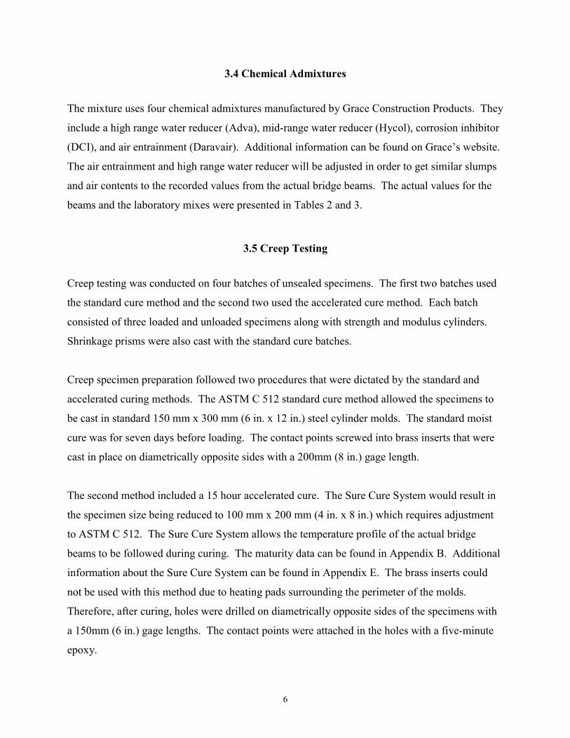
Table 4 Fresh Concrete Properties for the Standard Cure Batches ............................................................................... 4

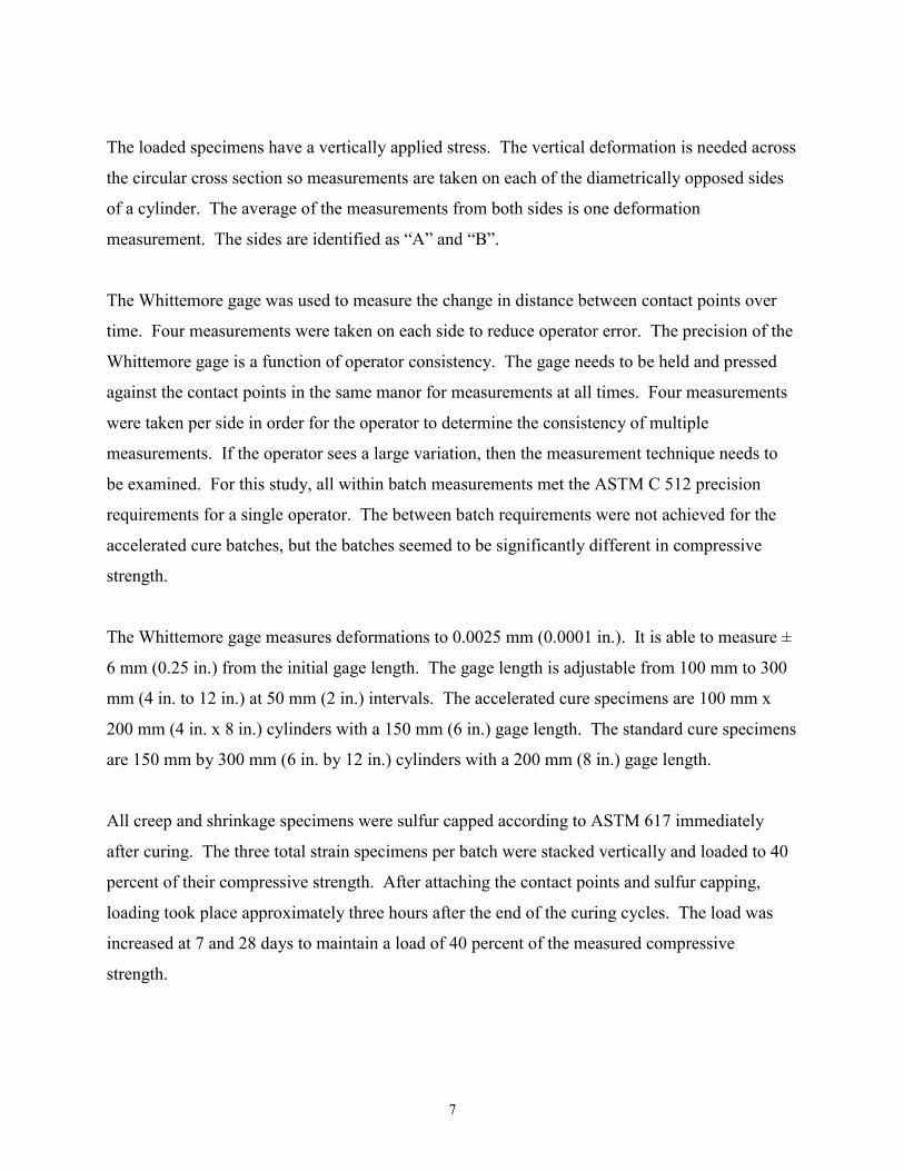
Table 5 Fresh Concrete Properties for the Accelerated Cure Batches .......................................................................... 5

Table 6 Standard Cure Experimental and Required Precision .................................................................................... 46

Table 7 Standard Cure Statistical Analysis of the Creep Microstrain. ........................................................................ 47

Table 8 Accelerated Cure Experimental and Required Precision ............................................................................... 47

Table 9 Accelerated Cure Statistical Analysis of the Creep Microstrain. ................................................................... 48

Table 10 Standard Cure Mean Residual Summary ..................................................................................................... 50

Table 11 Accelerated Cure Residual Summary .......................................................................................................... 51

Table 12 Standard Cure Average Total Strain Residuals (microstrain) ...................................................................... 54

Table 13 Standard Cure Average Shrinkage Residuals (microstrain) ......................................................................... 55

Table 14 Standard Cure Creep Strain Residuals Squared ........................................................................................... 56

Table 15 Accelerated Cure Average Total Strain Residuals (microstrain) ................................................................. 58

Table 16 Accelerated Cure Average Shrinkage Residuals (microstrain) .................................................................... 59

Table 17 Accelerated Cure Average Creep Strain Residuals (microstrain) ................................................................ 60

Table 18 Average Shrinkage Strain of Prisms (microstrain)....................................................................................... 61

Table 19 Standard Cure Prediction Model Rankings at 56 Days ................................................................................ 62

Table 20 Standard Cure Prediction Model Rankings at 250 Days .............................................................................. 62

Table 21 Accelerated Cure Prediction Model Rankings at 56 Days ........................................................................... 63

Table 22 Accelerated Cure Prediction Model Rankings at 250 Days ......................................................................... 63

Table 23 Standard Cure Shrinkage Prism Model Ranking ......................................................................................... 63

Table 24 GL2000 Recommended Cement Type factor............................................................................................... 64

Table 25 Experimental K factors and V/S ratios......................................................................................................... 65

Table 26 FHWA High-Performance Structural Concrete Grades (Myers) ................................................................. 81

Table 27 Multiple correlation coefficient for each part of the SAK model................................................................. 86

Table 28 Model limitations ......................................................................................................................................... 87

Table 29 Model parameters......................................................................................................................................... 87

Table 30 Aggregate Absorption and Specific Gravity .............................................................................................. 113

Table 31 Standard Cure Fresh Concrete Properties .................................................................................................. 113

Table 32 Accelerated Cure Fresh Concrete Properties.............................................................................................. 114

Table 33 Average Maturity before De-tensioning of Girders ................................................................................... 115

Table 34 Average Maturity at Removal from Match Cure System........................................................................... 115

ix

Table 35 Data from Standard Cure Batch 2 Measurements ...................................................................................... 131

Table 36 Data from Standard Cure Batch 3 Measurements ...................................................................................... 132

Table 37 Data from Accelerated Cure Batch 4 Measurements ................................................................................. 133

Table 38 Data from Accelerated Cure Batch 5 Measurements ................................................................................. 134

Table 39 Percent Length Change Measurements ...................................................................................................... 136

1

CHAPTER 1: INTRODUCTION

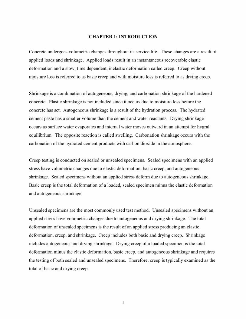
Concrete undergoes volumetric changes throughout its service life. These changes are a result of




Shrinkage is a combination of autogeneous, drying, and carbonation shrinkage of the hardened

concrete. Plastic shrinkage is not included since it occurs due to moisture loss before the

concrete has set. Autogeneous shrinkage is a result of the hydration process. The hydrated

cement paste has a smaller volume than the cement and water reactants. Drying shrinkage

occurs as surface water evaporates and internal water moves outward in an attempt for hygral

equilibrium. The opposite reaction is called swelling. Carbonation shrinkage occurs with the

carbonation of the hydrated cement products with carbon dioxide in the atmosphere.

Creep testing is conducted on sealed or unsealed specimens. Sealed specimens with an applied

stress have volumetric changes due to elastic deformation, basic creep, and autogeneous

shrinkage. Sealed specimens without an applied stress deform due to autogeneous shrinkage.

Basic creep is the total deformation of a loaded, sealed specimen minus the elastic deformation

and autogeneous shrinkage.

Unsealed specimens are the most commonly used test method. Unsealed specimens without an

applied stress have volumetric changes due to autogeneous and drying shrinkage. The total

deformation of unsealed specimens is the result of an applied stress producing an elastic

deformation, creep, and shrinkage. Creep includes both basic and drying creep. Shrinkage

includes autogeneous and drying shrinkage. Drying creep of a loaded specimen is the total

deformation minus the elastic deformation, basic creep, and autogeneous shrinkage and requires

the testing of both sealed and unsealed specimens. Therefore, creep is typically examined as the

total of basic and drying creep.

2

CHAPTER 2: PURPOSE AND SCOPE

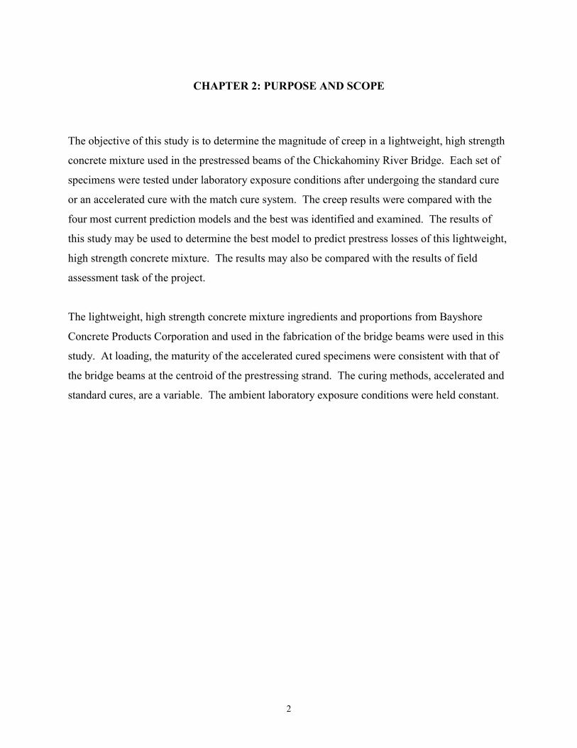
The objective of this study is to determine the magnitude of creep in a lightweight, high strength

concrete mixture used in the prestressed beams of the Chickahominy River Bridge. Each set of

specimens were tested under laboratory exposure conditions after undergoing the standard cure

or an accelerated cure with the match cure system. The creep results were compared with the

four most current prediction models and the best was identified and examined. The results of

this study may be used to determine the best model to predict prestress losses of this lightweight,

high strength concrete mixture. The results may also be compared with the results of field

assessment task of the project.

The lightweight, high strength concrete mixture ingredients and proportions from Bayshore

Concrete Products Corporation and used in the fabrication of the bridge beams were used in this

study. At loading, the maturity of the accelerated cured specimens were consistent with that of

the bridge beams at the centroid of the prestressing strand. The curing methods, accelerated and

standard cures, are a variable. The ambient laboratory exposure conditions were held constant.

3

CHAPTER 3: METHODS AND MATERIALS

3.1 Introduction

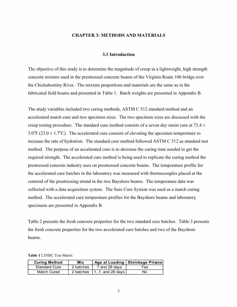
The objective of this study is to determine the magnitude of creep in a lightweight, high strength

concrete mixture used in the prestressed concrete beams of the Virginia Route 106 bridge over

the Chickahominy River. The mixture proportions and materials are the same as in the

fabricated field beams and presented in Table 1. Batch weights are presented in Appendix B.

The study variables included two curing methods, ASTM C 512 standard method and an

accelerated match cure and two specimen sizes. The two specimen sizes are discussed with the

creep testing procedure. The standard cure method consists of a seven day moist cure at 73.4 ±

3.0oF (23.0 ± 1.7oC). The accelerated cure consists of elevating the specimen temperature to

increase the rate of hydration. The standard cure method followed ASTM C 512 as standard test

method. The purpose of an accelerated cure is to decrease the curing time needed to get the

required strength. The accelerated cure method is being used to replicate the curing method the

prestressed concrete industry uses on prestressed concrete beams. The temperature profile for

the accelerated cure batches in the laboratory was measured with thermocouples placed at the

centroid of the prestressing strand in the two Bayshore beams. The temperature data was

collected with a data acquisition system. The Sure Cure System was used as a match curing

method. The accelerated cure temperature profiles for the Bayshore beams and laboratory

specimens are presented in Appendix B.

Table 2 presents the fresh concrete properties for the two standard cure batches. Table 3 presents

the fresh concrete properties for the two accelerated cure batches and two of the Bayshore

beams.

Table 1 LTHSC Test Matrix

Curing Method Mix Age at Loading Shrinkage PrismsStandard Cure 2 batches 7 and 28 days YesMatch Cured 2 batches 1, 7, and 28 days No

4

Table 2 Duration of weekly testing

Task

1. Standard Cure Creep Testing

2. Standard Cure Shrinkage Prism Testing

3. Accelerated Cure Creep Testing

Nov

-01

Dec

-01

Jan-

02

Feb-

02

Mar

-02

Apr

-02

May

-02

Jun-

02

Jul-0

2

Aug

-02

Sep

-02

Oct

-02

Nov

-02

Dec

-02

LTHSC Laboratory Testing

Table 3 Bayshore Mixture Proportions

Materials

Portland Cement (Type II) 451 lb. 268 kg.Slag Cement (Grade 120) 301 lb. 179 kg.Coarse Aggregate (lightweight) 696 lb. 413 kg.Coarse Aggregate (normal weight) 605 lb. 359 kg.Fine Aggregate (lightweight) 390 lb. 231 kg.Fine Aggregate (normal weight) 541 lb. 321 kg.Water 255 lb. 151 kg.AEA (Daravair) 12 oz. 355 ml.WR (Hycol) 22 oz. 651 ml.HRWR (Adva) 56 oz. 1656 ml.CI or Accel (DCI) 3 gal. 11.4 L

SSD weights per cubic yard

SSD weights per cubic meter

Table 4 Fresh Concrete Properties for the Standard Cure Batches

Fresh Concrete Properties LTHSC 2B LTHSC 3B

Slump, mm (in.) 165 (6.5) 140 (5.5)

Air Content (%) 6.5 5.5 Temperature, oC (oF) 26 (78) 26 (78)

Unit Weight, kg/m3 (pcf) 1880 (117.3) 1910 (119.1)

Yield 1.02 1.01 w/cm ratio 0.369 0.369 Curing Method Standard Standard

5

Table 5 Fresh Concrete Properties for the Accelerated Cure Batches

Fresh Concrete Properties

LTHSC 4B

LTHSC 5B

Bayshore BB1

Bayshore BB2

VDOT specs.

Slump, mm (in.) 100 (4.0) 150 (6.0) 180 (7) 215 (8.5) 0-100 (0-4)

Air Content (%) 6.0 7.1 5.5 6.0 3 – 6 Temperature, oC (oF) 24 (75) 24 (76) 21(70) 20 (68) ----

Unit Weight, kg/m3 (pcf) 1930 (120.3) 1875 (117.1) 1950 (122.0) 1900 (118.8) ----

Yield 1.00 1.02 0.98 1.01 ---- w/cm ratio 0.369 0.369 0.369 0.369 < 0.4 Curing Method Sure Cure Sure Cure Steam Steam N/A

3.2 Aggregate Properties

The concrete mixture has two fine and two coarse aggregates, a normal and lightweight

aggregate. The lightweight aggregate is both a fine and #67 expanded slate from the Carolina

Stalite Company. The normal weight aggregates are a natural sand and # 67 crushed diabase.

The specific gravity and absorption values for the aggregates were measured according to ASTM

C 127 and 128. The measured specific gravity and absorption values can be found in Appendix

B.

Carolina Stalite’s website includes reports from the laboratories of Law Engineering and

Environmental Services and Froechling & Robertson, Inc. that document the lightweight

aggregate meeting the requirements of ASTM C 330.

3.3 Cement Properties

The mixture includes a Type I/II Portland Cement and a ground granulated blast furnace slag

(GGBFS). The GGBFS is a Grade 120. Grade specifies the fineness of the mineral admixture,

which is related to the magnitude of hydraulic activity and potential strength. With a finer slag,

the increased surface area increases the rate of hydration. The Grade of GGBFS in this study is

constant.

6

3.4 Chemical Admixtures

The mixture uses four chemical admixtures manufactured by Grace Construction Products. They

include a high range water reducer (Adva), mid-range water reducer (Hycol), corrosion inhibitor

(DCI), and air entrainment (Daravair). Additional information can be found on Grace’s website.

The air entrainment and high range water reducer will be adjusted in order to get similar slumps

and air contents to the recorded values from the actual bridge beams. The actual values for the

beams and the laboratory mixes were presented in Tables 2 and 3.

3.5 Creep Testing

Creep testing was conducted on four batches of unsealed specimens. The first two batches used

the standard cure method and the second two used the accelerated cure method. Each batch

consisted of three loaded and unloaded specimens along with strength and modulus cylinders.

Shrinkage prisms were also cast with the standard cure batches.

Creep specimen preparation followed two procedures that were dictated by the standard and

accelerated curing methods. The ASTM C 512 standard cure method allowed the specimens to

be cast in standard 150 mm x 300 mm (6 in. x 12 in.) steel cylinder molds. The standard moist

cure was for seven days before loading. The contact points screwed into brass inserts that were

cast in place on diametrically opposite sides with a 200mm (8 in.) gage length.

The second method included a 15 hour accelerated cure. The Sure Cure System would result in

the specimen size being reduced to 100 mm x 200 mm (4 in. x 8 in.) which requires adjustment

to ASTM C 512. The Sure Cure System allows the temperature profile of the actual bridge

beams to be followed during curing. The maturity data can be found in Appendix B. Additional

information about the Sure Cure System can be found in Appendix E. The brass inserts could

not be used with this method due to heating pads surrounding the perimeter of the molds.

Therefore, after curing, holes were drilled on diametrically opposite sides of the specimens with

a 150mm (6 in.) gage lengths. The contact points were attached in the holes with a five-minute

epoxy.

7

The loaded specimens have a vertically applied stress. The vertical deformation is needed across

the circular cross section so measurements are taken on each of the diametrically opposed sides

of a cylinder. The average of the measurements from both sides is one deformation

measurement. The sides are identified as “A” and “B”.

The Whittemore gage was used to measure the change in distance between contact points over

time. Four measurements were taken on each side to reduce operator error. The precision of the

Whittemore gage is a function of operator consistency. The gage needs to be held and pressed

against the contact points in the same manor for measurements at all times. Four measurements

were taken per side in order for the operator to determine the consistency of multiple

measurements. If the operator sees a large variation, then the measurement technique needs to

be examined. For this study, all within batch measurements met the ASTM C 512 precision

requirements for a single operator. The between batch requirements were not achieved for the

accelerated cure batches, but the batches seemed to be significantly different in compressive

strength.

The Whittemore gage measures deformations to 0.0025 mm (0.0001 in.). It is able to measure ±

6 mm (0.25 in.) from the initial gage length. The gage length is adjustable from 100 mm to 300

mm (4 in. to 12 in.) at 50 mm (2 in.) intervals. The accelerated cure specimens are 100 mm x

200 mm (4 in. x 8 in.) cylinders with a 150 mm (6 in.) gage length. The standard cure specimens

are 150 mm by 300 mm (6 in. by 12 in.) cylinders with a 200 mm (8 in.) gage length.

All creep and shrinkage specimens were sulfur capped according to ASTM 617 immediately

after curing. The three total strain specimens per batch were stacked vertically and loaded to 40

percent of their compressive strength. After attaching the contact points and sulfur capping,

loading took place approximately three hours after the end of the curing cycles. The load was

increased at 7 and 28 days to maintain a load of 40 percent of the measured compressive

strength.

8

The load frames have been calibrated using a load cell, pressure gages, and strain gages.

Additional information is available in Appendix D.

Deformation measurements were taken immediately before and after loading or increasing the

load to record the elastic deformation. After loading, measurements were taken at 2 hours, 6

hours, and then daily for a week. Measurements were continued weekly thereafter. For

presentation, measurements are reported weekly up to 28 days and then once every four weeks.

Creep measurements were taken on two standard cure batches and two accelerated cure batches

for 329 and 251 days, respectively.

The strains were taken as the change in length at a given time divided by the initial length. Since

ASTM C512 does not specify the order to subtract the shrinkage strain from the total strain, the

three loaded and unloaded cylinders were paired based on corresponding strain magnitudes.

Therefore, the high, medium, and low total strains were subtracted from the high, medium, and

low shrinkage strains, respectively.

3.6 Shrinkage Testing

Shrinkage Prisms were cast and tested according ASTM C 157. The 75 mm x 75 mm x 280 mm

(3 in. x 3 in. x 11.25 in.) prisms were stored adjacent to the creep frames in the creep room at

73.4 ± 3 oF (23.0 ± 1.7oC) and 45 ± 4 % relative humidity. The relative humidity was slightly

lower than the specified 50 ± 4 % due to the room’s environmental control unit. A comparator

was used to take measurements according to ASTM 490-98. Measurements were taken on the

same time schedule as the creep testing.

3.7 Strength and Modulus Testing

Compressive and tensile strength cylinders and an elastic modulus cylinder were cast according

to ASTM C 192 for each batch. After curing, all strength and modulus specimens were sulfur

capped per ASTM 617 and stored with the creep and shrinkage specimens in the creep room.

9

The creep room temperature was 73.4 ± 3 oF (23.0 ± 1.7oC) and the relative humidity was 45 ± 4

%. The target relative humidity was 50 % ± 4 %.

Compressive strengths tests were conducted on 100 mm x 200 mm (4 in. x 8 in.) cylindrical

specimens according to ASTM C39. Each measurement is the mean of two tests. Compressive

strength measurements were taken at 7, 28, 56, and 90 days for the standard cure batches and at

1, 7, and 28 days for the accelerated cure batches. The Sure Cure System limited the number of

accelerated cure specimens that could be tested.

Splitting tensile strength tests were conducted according to ASTM C 496. Each strength

measurement is the mean of two tests. Tensile measurements were taken at 7 and 28 days for the

standard cure batches and at 17 hours and 28 days for the accelerated cure batches.

The modulus of elasticity was measured according to ASTM C 469. Measurements were

repeated at various times on one specimen per batch. The modulus of elasticity was measured on

150 mm x 300 mm (6 in. x 12 in.) and 100 mm x 200 mm (4 in. x 8 in.) cylinders for the

standard and accelerated cure batches, respectively. Measurements were taken at seven, 28, 56,

and 90 days for the standard cure batches and at one, seven, 28, 56, and 90 days for the

accelerated cure batches.

3.8 Thermal Coefficient The thermal coefficient for this mix was measured with the batch 2 shrinkage specimens after the

end of data collection. The strain measurements were taken at ambient conditions before and

after thermal measurements to insure that the strains were due to thermal conditions and not

moisture loss. Three 150 mm x 300 mm (6 in. x 12 in.) cylinders were subjected to temperatures

of 33oF to 120oF (0oC to 49oC) for three days at each temperature.

10

CHAPTER 4: RESULTS

4.1 Introduction

The compressive strength, tensile strength, modulus of elasticity, and thermal coefficient data for

both the lightweight high strength concrete (LTHSC) standard and accelerated cure batches are

summarized in the following sections. The standard and accelerated experimental total strain,

creep strain, and shrinkage strains per batch are presented. Whereas the measured strain values

are tabulated in Appendix F. Predicted values for the four models are also included. The

precision of the experimental values are examined as are the residuals of four prediction models.

The chapter concludes with the presentation of the standard cure, shrinkage prism results.

Each strength measurement is the average of two tested cylinders. Strength and modulus

specimens were stored in the same environmental conditions as the creep and shrinkage

specimens after the standard or accelerated cure regimens. The standard cure method was

applied to batches 2 (2B) and 3 (3B). The accelerated cure method was applied to batches 4 (4B)

and 5 (5B). Batch 1 (1B) was discarded due to an excessive air content.

Strength and modulus measurements for the LTHSC bridge beams (BB1 and BB2) are also

presented. The compressive strength measurements are reported by Bayshore Concrete

Products. Splitting tensile strength and modulus of elasticity were measured by VTRC.

The mixture proportions and fresh concrete properties are provided in Appendix B.

11

4.2 Compressive Strength

4.2.1 Standard Cure

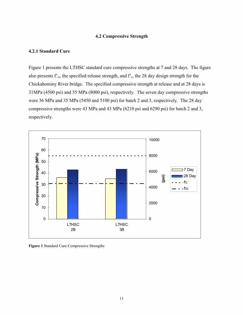
Figure 1 presents the LTHSC standard cure compressive strengths at 7 and 28 days. The figure

also presents f’ci, the specified release strength, and f’c, the 28 day design strength for the

Chickahominy River bridge. The specified compressive strength at release and at 28 days is

31MPa (4500 psi) and 55 MPa (8000 psi), respectively. The seven day compressive strengths

were 36 MPa and 35 MPa (5450 and 5100 psi) for batch 2 and 3, respectively. The 28 day

compressive strengths were 43 MPa and 43 MPa (6210 psi and 6290 psi) for batch 2 and 3,

respectively.

0

10

20

30

40

50

60

70

LTHSC2B

LTHSC3B

Com

pres

sive

Stre

ngth

(MPa

)

0

2000

4000

6000

8000

10000

(psi

)7 Day 28 Dayf'cf'ci

Figure 1 Standard Cure Compressive Strengths

12

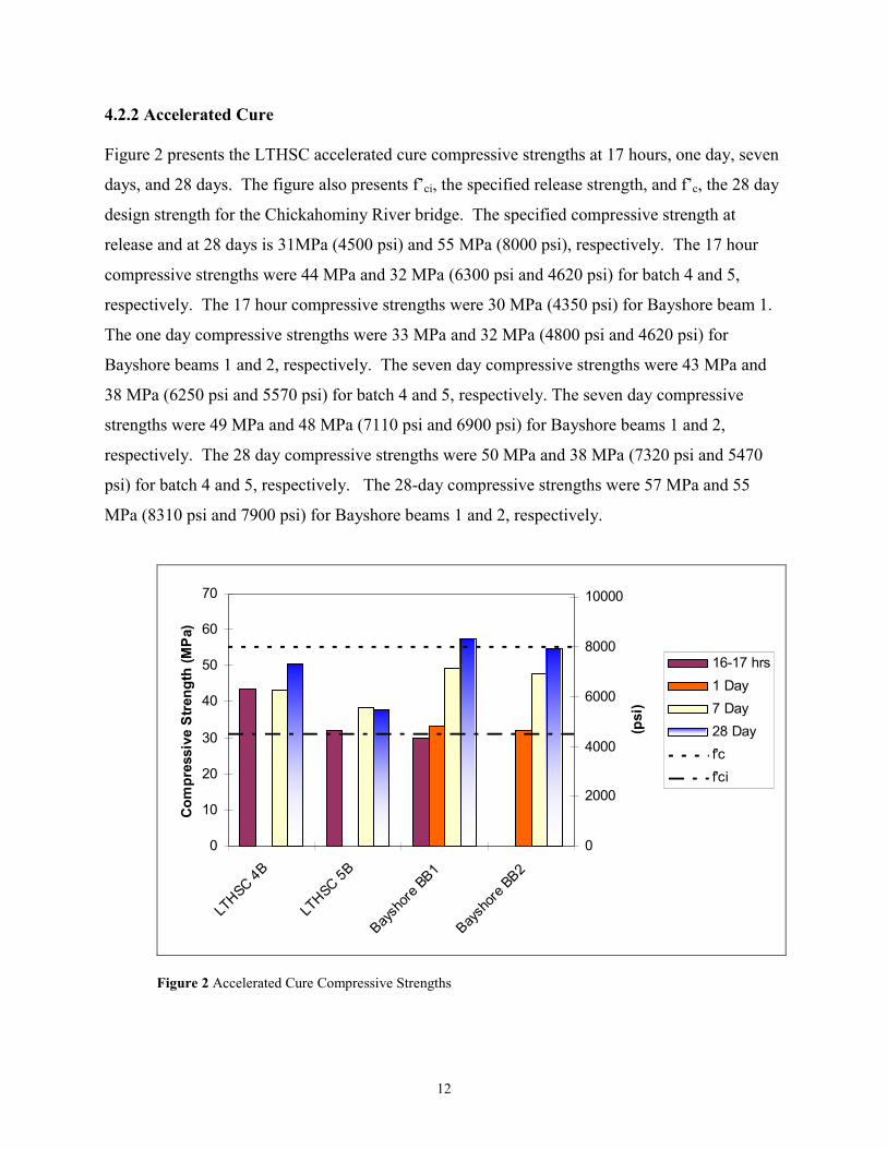
4.2.2 Accelerated Cure Figure 2 presents the LTHSC accelerated cure compressive strengths at 17 hours, one day, seven

days, and 28 days. The figure also presents f’ci, the specified release strength, and f’c, the 28 day

design strength for the Chickahominy River bridge. The specified compressive strength at

release and at 28 days is 31MPa (4500 psi) and 55 MPa (8000 psi), respectively. The 17 hour

compressive strengths were 44 MPa and 32 MPa (6300 psi and 4620 psi) for batch 4 and 5,

respectively. The 17 hour compressive strengths were 30 MPa (4350 psi) for Bayshore beam 1.

The one day compressive strengths were 33 MPa and 32 MPa (4800 psi and 4620 psi) for

Bayshore beams 1 and 2, respectively. The seven day compressive strengths were 43 MPa and

38 MPa (6250 psi and 5570 psi) for batch 4 and 5, respectively. The seven day compressive

strengths were 49 MPa and 48 MPa (7110 psi and 6900 psi) for Bayshore beams 1 and 2,

respectively. The 28 day compressive strengths were 50 MPa and 38 MPa (7320 psi and 5470

psi) for batch 4 and 5, respectively. The 28-day compressive strengths were 57 MPa and 55

MPa (8310 psi and 7900 psi) for Bayshore beams 1 and 2, respectively.

0

10

20

30

40

50

60

70

LTHSC 4B

LTHSC 5B

Baysh

ore BB1

Baysh

ore BB2

Com

pres

sive

Stre

ngth

(MPa

)

0

2000

4000

6000

8000

10000

(psi

)

16-17 hrs1 Day 7 Day 28 Dayf'cf'ci

Figure 2 Accelerated Cure Compressive Strengths

13

4.3 Tensile Strength

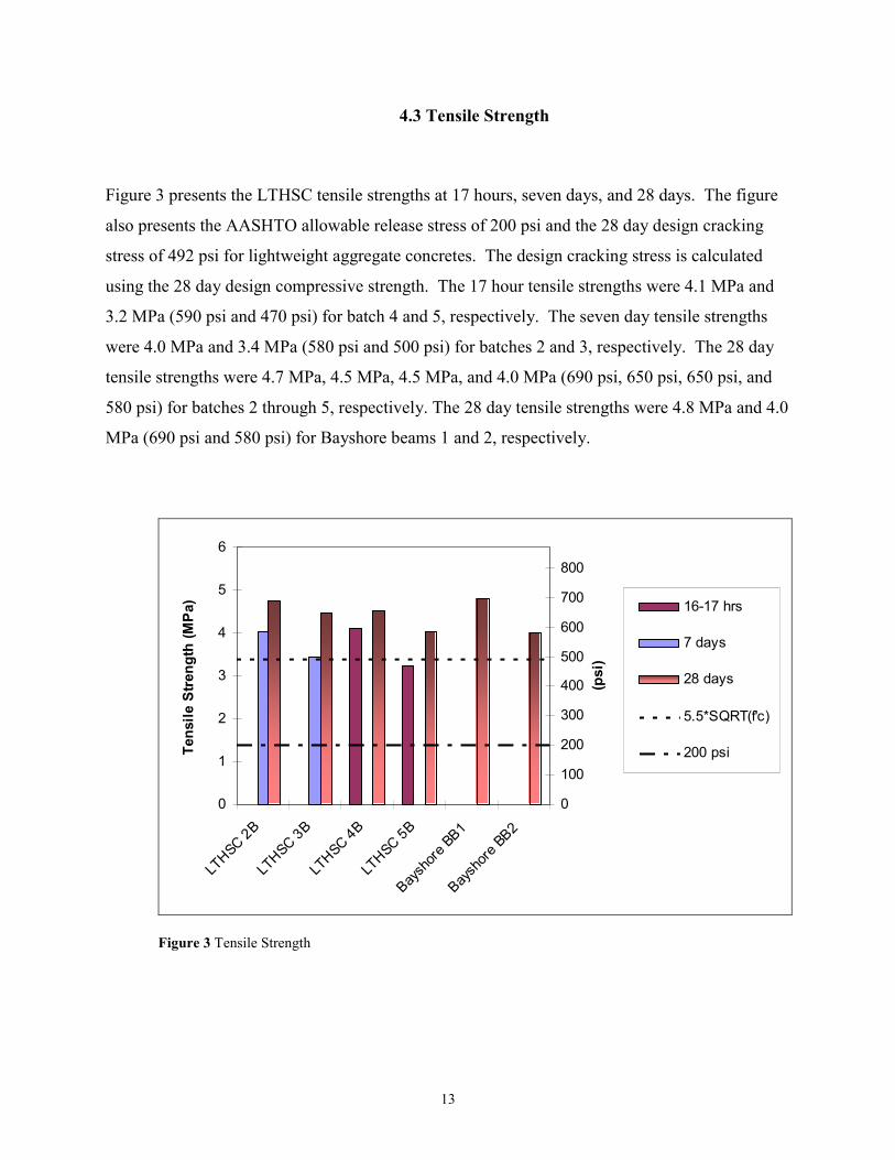
Figure 3 presents the LTHSC tensile strengths at 17 hours, seven days, and 28 days. The figure

also presents the AASHTO allowable release stress of 200 psi and the 28 day design cracking

stress of 492 psi for lightweight aggregate concretes. The design cracking stress is calculated

using the 28 day design compressive strength. The 17 hour tensile strengths were 4.1 MPa and

3.2 MPa (590 psi and 470 psi) for batch 4 and 5, respectively. The seven day tensile strengths

were 4.0 MPa and 3.4 MPa (580 psi and 500 psi) for batches 2 and 3, respectively. The 28 day

tensile strengths were 4.7 MPa, 4.5 MPa, 4.5 MPa, and 4.0 MPa (690 psi, 650 psi, 650 psi, and

580 psi) for batches 2 through 5, respectively. The 28 day tensile strengths were 4.8 MPa and 4.0

MPa (690 psi and 580 psi) for Bayshore beams 1 and 2, respectively.

0

1

2

3

4

5

6

LTHSC 2B

LTHSC 3B

LTHSC 4B

LTHSC 5B

Baysh

ore BB1

Baysh

ore BB2

Tens

ile S

treng

th (M

Pa)

0

100

200

300

400

500

600

700

800

(psi

)16-17 hrs

7 days

28 days

5.5*SQRT(f'c)

200 psi

Figure 3 Tensile Strength

14

4.4 Modulus of Elasticity

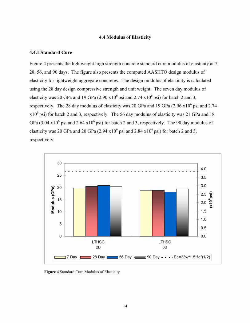
4.4.1 Standard Cure Figure 4 presents the lightweight high strength concrete standard cure modulus of elasticity at 7,

28, 56, and 90 days. The figure also presents the computed AASHTO design modulus of

elasticity for lightweight aggregate concretes. The design modulus of elasticity is calculated

using the 28 day design compressive strength and unit weight. The seven day modulus of

elasticity was 20 GPa and 19 GPa (2.90 x106 psi and 2.74 x106 psi) for batch 2 and 3,

respectively. The 28 day modulus of elasticity was 20 GPa and 19 GPa (2.96 x106 psi and 2.74

x106 psi) for batch 2 and 3, respectively. The 56 day modulus of elasticity was 21 GPa and 18

GPa (3.04 x106 psi and 2.64 x106 psi) for batch 2 and 3, respectively. The 90 day modulus of

elasticity was 20 GPa and 20 GPa (2.94 x106 psi and 2.84 x106 psi) for batch 2 and 3,

respectively.

0

5

10

15

20

25

30

LTHSC2B

LTHSC3B

Mod

ulus

(GPa

)

0.0

0.5

1.0

1.5

2.0

2.5

3.0

3.5

4.0

(x10

6 psi)

7 Day 28 Day 56 Day 90 Day Ec=33w^1.5*f'c (̂1/2)

Figure 4 Standard Cure Modulus of Elasticity

15

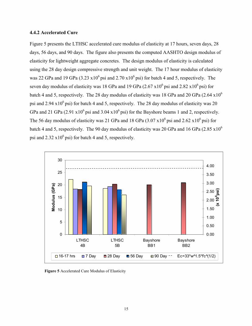
4.4.2 Accelerated Cure Figure 5 presents the LTHSC accelerated cure modulus of elasticity at 17 hours, seven days, 28

days, 56 days, and 90 days. The figure also presents the computed AASHTO design modulus of

elasticity for lightweight aggregate concretes. The design modulus of elasticity is calculated

using the 28 day design compressive strength and unit weight. The 17 hour modulus of elasticity

was 22 GPa and 19 GPa (3.23 x106 psi and 2.70 x106 psi) for batch 4 and 5, respectively. The

seven day modulus of elasticity was 18 GPa and 19 GPa (2.67 x106 psi and 2.82 x106 psi) for

batch 4 and 5, respectively. The 28 day modulus of elasticity was 18 GPa and 20 GPa (2.64 x106

psi and 2.94 x106 psi) for batch 4 and 5, respectively. The 28 day modulus of elasticity was 20

GPa and 21 GPa (2.91 x106 psi and 3.04 x106 psi) for the Bayshore beams 1 and 2, respectively.

The 56 day modulus of elasticity was 21 GPa and 18 GPa (3.07 x106 psi and 2.62 x106 psi) for

batch 4 and 5, respectively. The 90 day modulus of elasticity was 20 GPa and 16 GPa (2.85 x106

psi and 2.32 x106 psi) for batch 4 and 5, respectively.

0

5

10

15

20

25

30

LTHSC4B

LTHSC5B

BayshoreBB1

BayshoreBB2

Mod

ulus

(GPa

)

0.00

0.50

1.00

1.50

2.00

2.50

3.00

3.50

4.00

(x 1

06 psi)

16-17 hrs 7 Day 28 Day 56 Day 90 Day Ec=33*w^1.5*f'c (̂1/2)

Figure 5 Accelerated Cure Modulus of Elasticity

16

4.5 Thermal Coefficient The coefficient of thermal expansion for the LTHSC mixture was found to be 5.3 microstrain per oF (9.5 microstrain per oC) with a confidence interval of ± 0.13 microstrain microstrain per oF

(±0.24 microstrain per oC).

4.6 Experimental and Predicted Strains

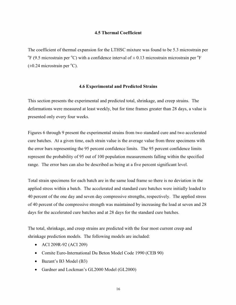
This section presents the experimental and predicted total, shrinkage, and creep strains. The

deformations were measured at least weekly, but for time frames greater than 28 days, a value is

presented only every four weeks.

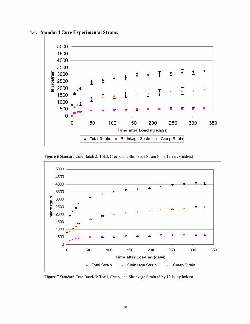
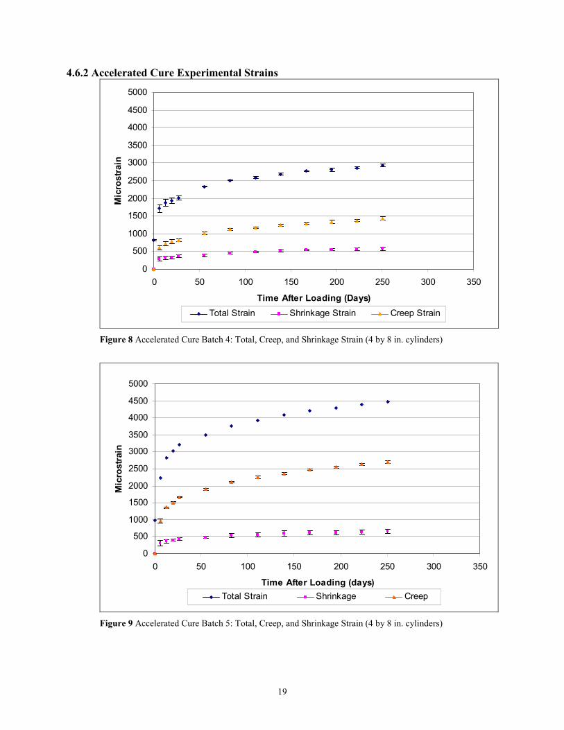
Figures 6 through 9 present the experimental strains from two standard cure and two accelerated

cure batches. At a given time, each strain value is the average value from three specimens with

the error bars representing the 95 percent confidence limits. The 95 percent confidence limits

represent the probability of 95 out of 100 population measurements falling within the specified

range. The error bars can also be described as being at a five percent significant level.

Total strain specimens for each batch are in the same load frame so there is no deviation in the

applied stress within a batch. The accelerated and standard cure batches were initially loaded to

40 percent of the one day and seven day compressive strengths, respectively. The applied stress

of 40 percent of the compressive strength was maintained by increasing the load at seven and 28

days for the accelerated cure batches and at 28 days for the standard cure batches.

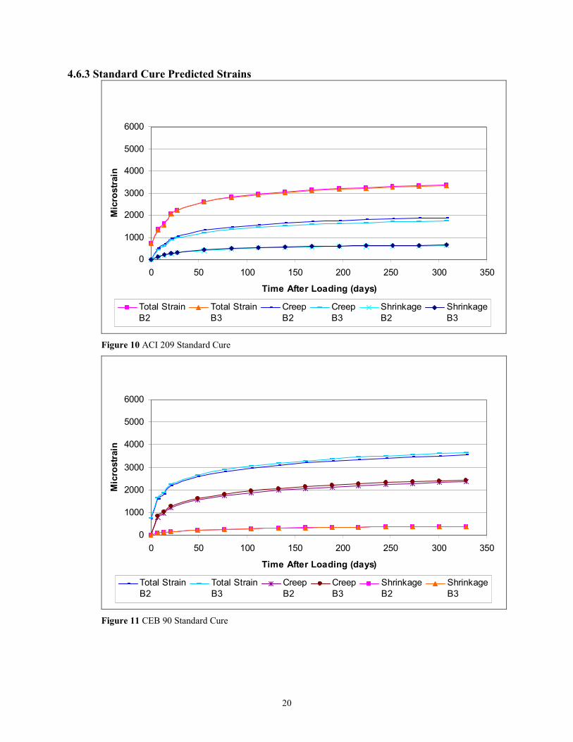
The total, shrinkage, and creep strains are predicted with the four most current creep and

shrinkage prediction models. The following models are included:

• ACI 209R-92 (ACI 209)

• Comite Euro-International Du Beton Model Code 1990 (CEB 90)

• Bazant’s B3 Model (B3)

• Gardner and Lockman’s GL2000 Model (GL2000)

17

The SAK model by Sakata was also considered, but was not included because of the limitations

in the scope of mixtures used during model development and the age of loading for accelerated

curing.

ACI 209 model was applied when predicting prestressed concrete losses for the Virginia Route

106 bridge over the Chickahominy River.

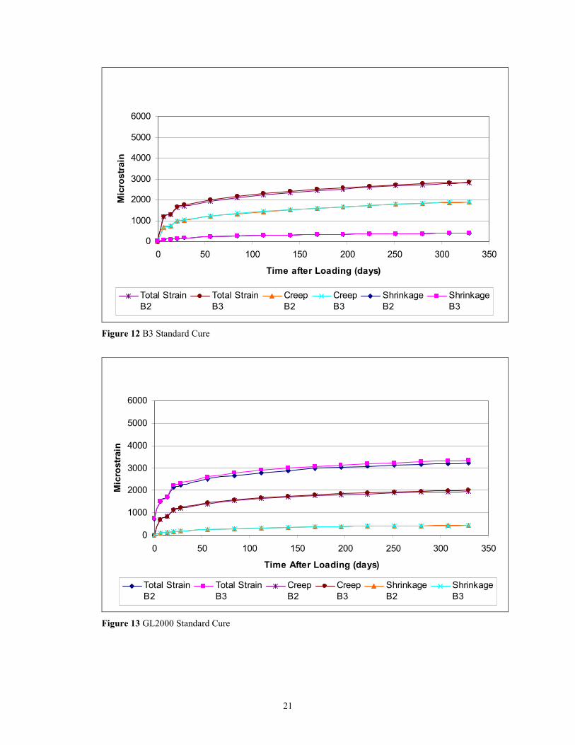
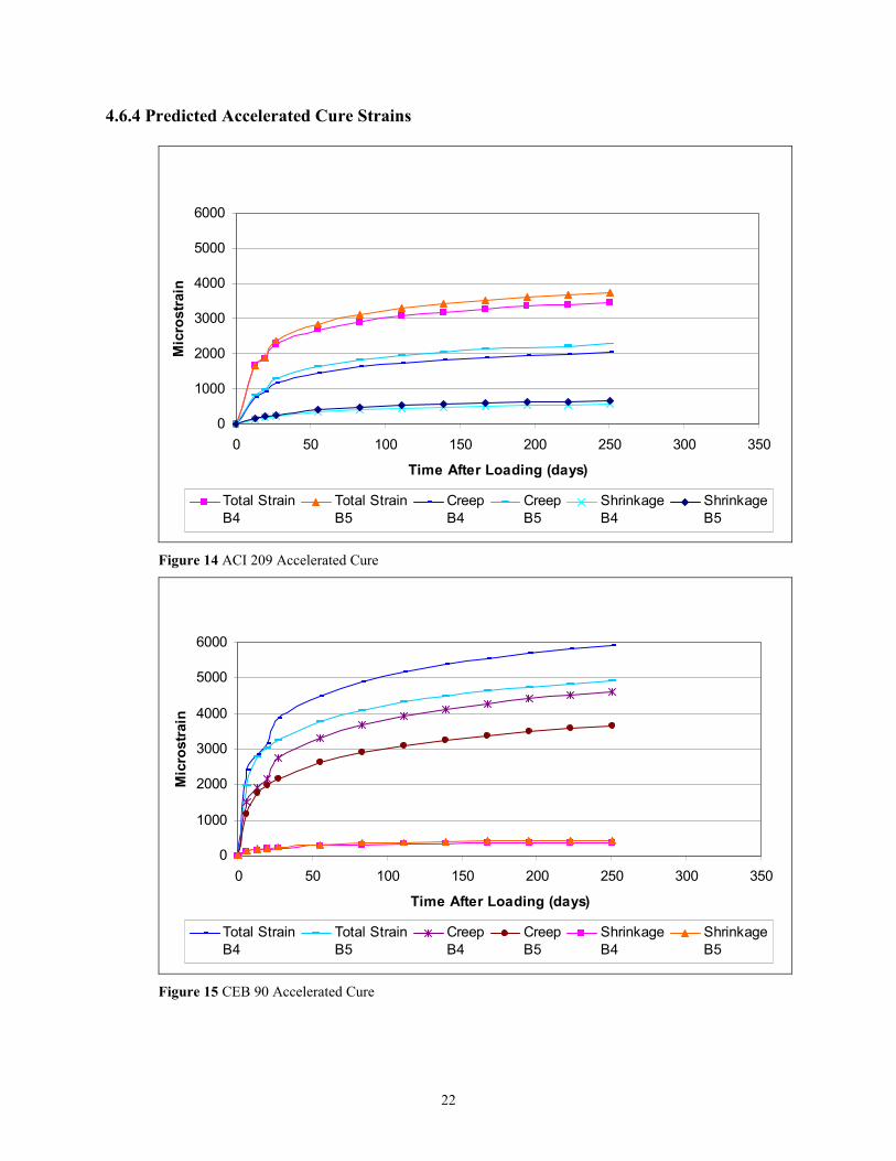
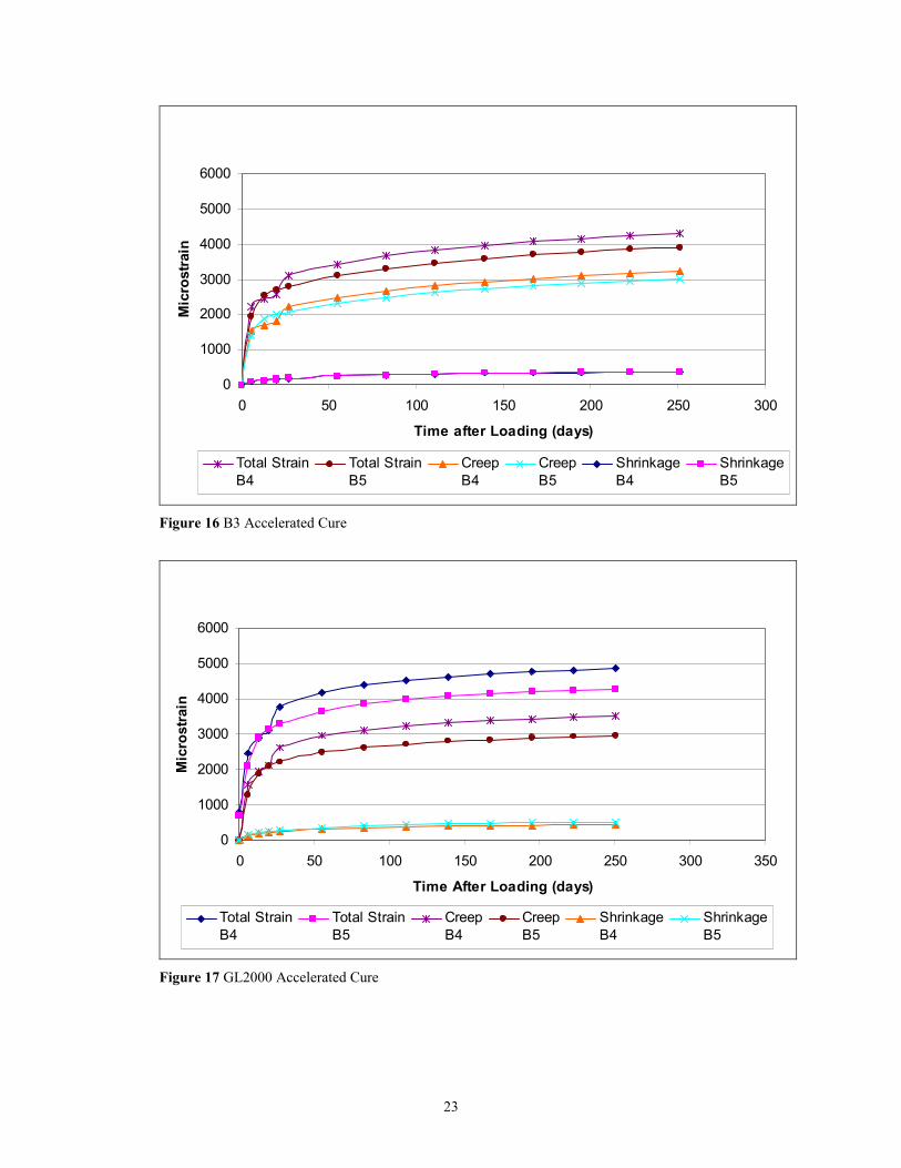
Figures 10 through 17 present the predicted total, shrinkage, and creep strains. The values are

predicted using the experimentally measured compressive strengths and modulus of elasticity for

each batch. If the LTHSC design strength was used, the elastic strain would have been under

predicted based on the measured values and current prediction equations. Time dependent

deformation would also be under predicted based on the strength. A strong cement paste matrix

is more resistant to time dependent losses than a weaker matrix.

Model details are presented in Appendix A.

18

4.6.1 Standard Cure Experimental Strains

0500

100015002000250030003500400045005000

0 50 100 150 200 250 300 350Time after Loading (days)

Mic

rost

rain

Total Strain Shrinkage Strain Creep Strain

Figure 6 Standard Cure Batch 2: Total, Creep, and Shrinkage Strain (6 by 12 in. cylinders)

0

500

1000

1500

2000

2500

3000

3500

4000

4500

5000

0 50 100 150 200 250 300 350

Time after Loading (days)

Mic

rost

rain


Figure 7 Standard Cure Batch 3: Total, Creep, and Shrinkage Strain (6 by 12 in. cylinders)

19

4.6.2 Accelerated Cure Experimental Strains

0

500

1000

1500

2000

2500

3000

3500

4000

4500

5000

0 50 100 150 200 250 300 350

Time After Loading (Days)

Mic

rost

rain


Figure 8 Accelerated Cure Batch 4: Total, Creep, and Shrinkage Strain (4 by 8 in. cylinders)

0

500

1000

1500

2000

2500

3000

3500

4000

4500

5000

0 50 100 150 200 250 300 350

Time After Loading (days)

Mic

rost

rain

Total Strain Shrinkage Creep

Figure 9 Accelerated Cure Batch 5: Total, Creep, and Shrinkage Strain (4 by 8 in. cylinders)

20

4.6.3 Standard Cure Predicted Strains

0

1000

2000

3000

4000

5000

6000

0 50 100 150 200 250 300 350


Mic

rost

rain

Total StrainB2

Total StrainB3

CreepB2

CreepB3

ShrinkageB2

ShrinkageB3

Figure 10 ACI 209 Standard Cure

0

1000

2000

3000

4000

5000

6000

0 50 100 150 200 250 300 350


Mic

rost

rain

Total StrainB2

Total StrainB3

CreepB2

CreepB3

ShrinkageB2

ShrinkageB3

Figure 11 CEB 90 Standard Cure

21

0

1000

2000

3000

4000

5000

6000

0 50 100 150 200 250 300 350


Mic

rost

rain

Total StrainB2

Total StrainB3

CreepB2

CreepB3

ShrinkageB2

ShrinkageB3

Figure 12 B3 Standard Cure

0

1000

2000

3000

4000

5000

6000

0 50 100 150 200 250 300 350


Mic

rost

rain

Total StrainB2

Total StrainB3

CreepB2

CreepB3

ShrinkageB2

ShrinkageB3

Figure 13 GL2000 Standard Cure

22

4.6.4 Predicted Accelerated Cure Strains

0

1000

2000

3000

4000

5000

6000

0 50 100 150 200 250 300 350


Mic

rost

rain

Total StrainB4

Total StrainB5

CreepB4

CreepB5

ShrinkageB4

ShrinkageB5

Figure 14 ACI 209 Accelerated Cure

0

1000

2000

3000

4000

5000

6000

0 50 100 150 200 250 300 350


Mic

rost

rain

Total StrainB4

Total StrainB5

CreepB4

CreepB5

ShrinkageB4

ShrinkageB5

Figure 15 CEB 90 Accelerated Cure

23

0

1000

2000

3000

4000

5000

6000

0 50 100 150 200 250 300


Mic

rost

rain

Total StrainB4

Total StrainB5

CreepB4

CreepB5

ShrinkageB4

ShrinkageB5

Figure 16 B3 Accelerated Cure

0

1000

2000

3000

4000

5000

6000

0 50 100 150 200 250 300 350


Mic

rost

rain

Total StrainB4

Total StrainB5

CreepB4

CreepB5

ShrinkageB4

ShrinkageB5

Figure 17 GL2000 Accelerated Cure

24

4.7 Prediction Model Residuals

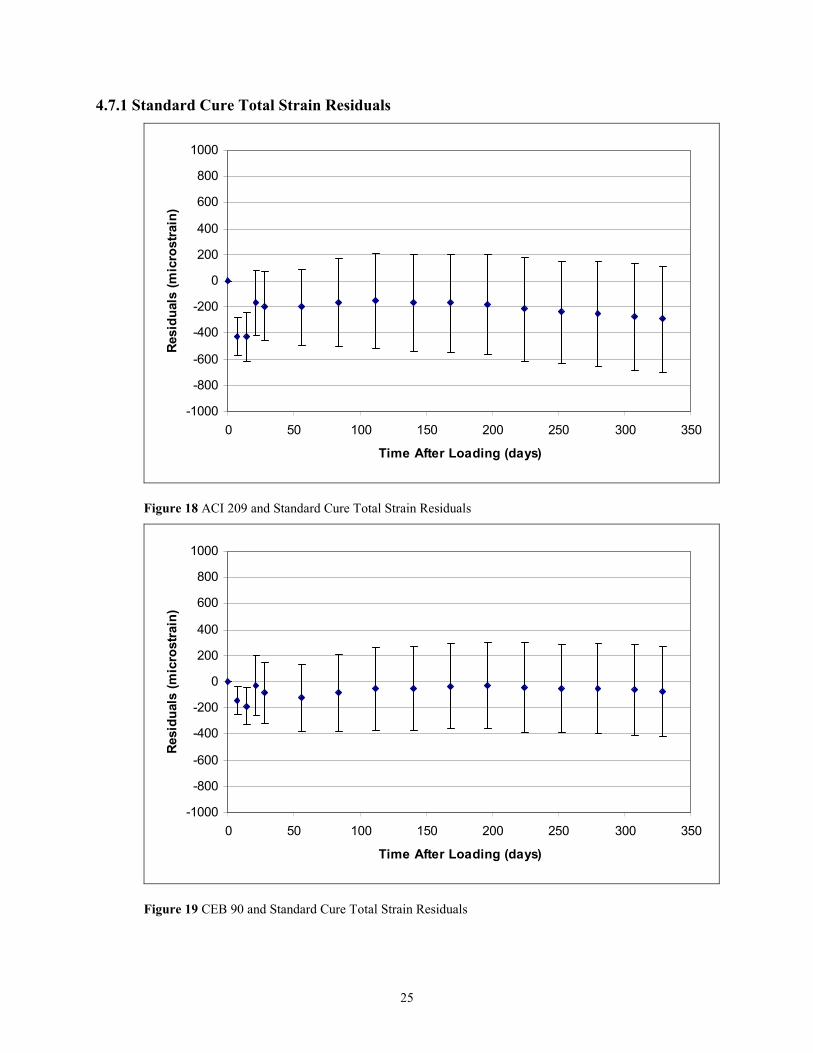
A residual is the difference between a model and the experimental value at a given time.

Residuals identify a model as either over predicting, a positive value, or under predicting, a

negative value. The residuals are calculated as the predicted model mean for a batch minus the

experimental value for a test specimen at a given time.

Figures 18 through 39 present the residuals plotted over time. The residuals are plotted as the

mean and the 95 percent confidence limits at the given test time. The standard cure residuals are

for batches 2 and 3 combined for a total of six test values. Whereas the accelerated cure

residuals are for batches 4 and 5 separately.

25

4.7.1 Standard Cure Total Strain Residuals

-1000

-800

-600

-400

-200

0

200

400

600

800

1000

0 50 100 150 200 250 300 350


Resi

dual

s (m

icro

stra

in)

Figure 18 ACI 209 and Standard Cure Total Strain Residuals

-1000

-800

-600

-400

-200

0

200

400

600

800

1000

0 50 100 150 200 250 300 350


Resi

dual

s (m

icro

stra

in)

Figure 19 CEB 90 and Standard Cure Total Strain Residuals

26

-1500

-1000

-500

0

500

1000

0 50 100 150 200 250 300 350


Resi

dual

s (m

icro

stra

in)

Figure 20 B3 and Standard Cure Total Strain Residuals

-1000

-800

-600

-400

-200

0

200

400

600

800

1000

0 50 100 150 200 250 300 350


Resi

dual

s (m

icro

stra

in)

Figure 21 GL2000 and Standard Cure Total Strain Residuals

27

4.7.2 Standard Cure Shrinkage Strain Residuals

-400

-300

-200

-100

0

100

200

300

400

0 50 100 150 200 250 300 350


Resi

dual

s (m

icro

stra

in)

Figure 22 ACI 209 and Standard Cure Shrinkage Residuals

-400

-300

-200

-100

0

100

200

300

400

0 50 100 150 200 250 300 350


Resi

dual

s (m

icro

stra

in)

Figure 23 CEB 90 and Standard Cure Shrinkage Residuals

28

-400

-300

-200

-100

0

100

200

300

400

0 50 100 150 200 250 300 350


Resi

dual

s (m

icro

stra

in)

Figure 24 B3 and Standard Cure Shrinkage Residuals

-400

-300

-200

-100

0

100

200

300

400

0 50 100 150 200 250 300 350


Resi

dual

s (m

icro

stra

in)

Figure 25 GL2000 and Standard Cure Shrinkage Residuals

29

4.7.3 Standard Cure Creep Strain Residuals

-1000

-800

-600

-400

-200

0

200

400

600

800

1000

0 50 100 150 200 250 300 350


Resi

dual

s (m

icro

stra

in)

Figure 26 ACI 209 and Standard Cure Creep Residuals

-1000

-800

-600

-400

-200

0

200

400

600

800

1000

0 50 100 150 200 250 300 350


Resi

dual

s (m

icro

stra

in)

Figure 27 CEB 90 and Standard Cure Creep Residuals

30

-1000

-800

-600

-400

-200

0

200

400

600

800

1000

0 50 100 150 200 250 300 350


Resi

dual

s (m

icro

stra

in)

Figure 28 B3 and Standard Cure Creep Residuals

-1000

-800

-600

-400

-200

0

200

400

600

800

1000

0 50 100 150 200 250 300 350


Resi

dual

s (m

icro

stra

in)

Figure 29 GL2000 and Standard Cure Creep Residuals

31

4.7.4 Accelerated Cure Total Strain Residuals

-1500

-1000

-500

0

500

1000

0 50 100 150 200 250 300 350


Resi

dual

s (m

icro

stra

in)

B4B5

Figure 30 ACI 209 and Accelerated Cure Total Strain Residuals per Batch

-1000

-500

0

500

1000

1500

2000

2500

3000

3500

0 50 100 150 200 250 300 350


Resi

dual

s (m

icro

stra

in)

B4B5

Figure 31 CEB 90 and Accelerated Cure Total Strain Residuals per Batch

32

-1000

-500

0

500

1000

1500

2000

0 50 100 150 200 250 300 350


Resi

dual

s (m

icro

stra

in)

B4B5

Figure 32 B3 and Accelerated Cure Total Strain Residuals per Batch

-1000

-500

0

500

1000

1500

2000

2500

0 50 100 150 200 250 300 350


Resi

dual

s (m

icro

stra

in)

B4B5

Figure 33 GL2000 and Accelerated Cure Total Strain Residuals per Batch

33

4.7.5 Accelerated Cure Shrinkage Strain Residuals

-400

-300

-200

-100

0

100

200

300

400

0 50 100 150 200 250 300 350


Resi

dual

s (m

icro

stra

in)

Figure 34 ACI 209 and Accelerated Cure Shrinkage Residuals

-400

-300

-200

-100

0

100

200

300

400

0 50 100 150 200 250 300 350


Resi

dual

s (m

icro

stra

in)

Figure 35 CEB 90 and Accelerated Cure Shrinkage Residuals

34

-400

-300

-200

-100

0

100

200

300

400

0 50 100 150 200 250 300 350


Resi

dual

s (m

icro

stra

in)

Figure 36 B3 and Accelerated Cure Shrinkage Residuals

-400

-300

-200

-100

0

100

200

300

400

0 50 100 150 200 250 300 350


Resi

dual

s (m

icro

stra

in)

Figure 37 GL2000 and Accelerated Cure Shrinkage Residuals

35

4.7.6 Accelerated Cure Creep Strain Residuals

-1000

-800

-600

-400

-200

0

200

400

600

800

1000

0 50 100 150 200 250 300 350


Resi

dual

s (m

icro

stra

in)

B4B5

Figure 38 ACI 209 and Accelerated Cure Creep Strain Residuals per Batch

-1000

-500

0

500

1000

1500

2000

2500

3000

3500

0 50 100 150 200 250 300 350


Resi

dual

s (m

icro

stra

in)

B4B5

Figure 39 CEB 90 and Accelerated Cure Creep Strain Residuals per Batch

36

-1000

-500

0

500

1000

1500

2000

0 50 100 150 200 250 300 350


Resi

dual

s (m

icro

stra

in)

B4B5

Figure 40 B3 and Accelerated Cure Creep Strain Residuals per Batch

-1000

-500

0

500

1000

1500

2000

2500

0 50 100 150 200 250 300 350


Resi

dual

s (m

icro

stra

in)

B4B5

Figure 41 GL2000 and Accelerated Cure Creep Strain Residuals per Batch

37

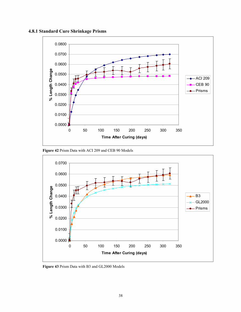
4.8 Shrinkage Prisms

Three 75 mm x 75 mm x 285 mm (3 in. x 3 in. x 11.25 in.) shrinkage prisms were made for each

standard cure batch per ASTM C157. Shrinkage prisms cannot be cast with the Sure Cure

system currently. The shrinkage was calculated as percent shrinkage. Percent shrinkage is

equivalent to microstrain x 10-4.

Figure 42 presents the mean percent length change with 95 percent confidence limits and the

ACI 209 and the CEB 90 predictions. The ACI 209 model initially under predicts shrinkage and

over predicts after 50 days. The CEB 90 model is the best early age predictor, but under predicts

shrinkage after 28 days.

Figure 43 presents the percent length change for the shrinkage prisms with 95 percent confidence

limits and the B3 and GL2000 predictions. The B3 model initially under predicts shrinkage up

to 80 days and then falls within the prisms 95 percent confidence limits. The GL2000 model

under predicts shrinkage throughout drying. The GL2000 model is examined in a K factor

sensitivity analysis for the cement type.

38

4.8.1 Standard Cure Shrinkage Prisms

0.0000

0.0100

0.0200

0.0300

0.0400

0.0500

0.0600

0.0700

0.0800

0 50 100 150 200 250 300 350

Time After Curing (days)

% L

engt

h Ch

ange

ACI 209CEB 90Prisms

Figure 42 Prism Data with ACI 209 and CEB 90 Models

0.0000

0.0100

0.0200

0.0300

0.0400

0.0500

0.0600

0.0700

0 50 100 150 200 250 300 350


% L

engt

h Ch

ange

B3GL2000Prisms

Figure 43 Prism Data with B3 and GL2000 Models

39

CHAPTER 5: DISCUSSION AND ANALYSIS

5.1 Introduction

This chapter discusses physical properties of the LTHSC mixture and an analysis of the four

prediction models. The physical properties include the compressive strength, tensile strength,

and modulus of elasticity. The model analysis includes the residual squared method, a sensitivity

analysis, and the best prediction model is identified.

5.2 Compressive Strength

Figure 1 presents the LTHSC standard cure compressive strengths. The strengths of the two

standard cure batches at seven and 28 days is not significantly different.

Figure 2 presents the accelerated cure compressive strengths for the two LTHSC batches and the

Bayshore bridge beams. The LTHSC compressive strengths immediately after curing are

approximately the same or greater than the Bayshore results. The Bayshore specimens had a

larger strength increase with time. The Bayshore specimens were stored outside with the beams.

The environmental conditions in this area are relatively humid considering the plant is

surrounded by water on three sides. These conditions appear to have allowed hydration to

continue. After curing, the LTHSC specimens were exposed to a drying environment of 45%

relative humidity, as were the loaded and unloaded specimens.

The strength gain after curing is similar between the two standard cure batches. Batch 4 is

approximately 35 percent stronger than batch 5 after curing. The accelerated curing process has

increased the variability of the batches. Maturity is calculated as the area under the temperature-

time curve from 14oF or -10oC (Mehta). The maturity difference between the Bayshore Beams is

20 percent, 1000 and 830oC-hr. The maturity of batch 4 (1040 oC-hr) is 10 percent higher than

batch 5 (940 oC-hr) since it had two hours less of a preset before the temperature increase began.

This was due to an experimental error with the match cure system. The maturity of batch 4 is

40

close to that of beam 1. The target maturity was to be the average of the two beams Maturity

data is presented in Appendix B.

An additional difference between batches 4 and 5 is the unit weight of 1930 kg/m3 and 1875

kg/m3 (120.3 pcf and 117.1 pcf), respectively. The Bayshore beams had unit weights of 1955

kg/m3 and 1905 kg/m3 (122.0pcf and 118.8 pcf) for BB1 and BB2, respectively. There is a

variability between batches or beams, but this is similar in the laboratory and in the field. The

variability in unit weight corresponds with the variation in compressive strengths. A higher unit

weight results in a higher compressive strength between the accelerated cure batches and

between the beam beams.

The accelerated cure between batch strength differences are directly related to the creep strains

not meeting the ASTM precision requirements. If the maturity and/or unit weight is significantly

different then creep behavior is likely to be significantly different between batches.

Neither the accelerated or the standard cure batches reached the 55 Mpa (8000 psi) design

strength. This can be attributed to the specimens being placed in a drying environment, which

slowed hydration and strength gain. The Bayshore specimens reached the required strength and

were stored outside with the beams in a relatively humid environment. Figure 1 and 2 shows the

measured compressive strengths at loading or release. The standard cure, accelerated cure, and

bridge beam specimens reached the required release strength of 31 MPa (4500 psi) at loading or

release.

5.3 Tensile Strength

Figure 3 presents the tensile strength data for the four batches and the bridge beams. The

LTHSC 28 day tensile strength measurements are within the range of the Bayshore

measurements. There is a strong correlation between the tensile strength being equivalent to one

tenth of the compressive strength for the LTHSC specimens. The Bayshore specimens had

higher compressive strengths, but the tensile strengths were not significantly different from the

LTHSC specimens. Both the laboratory and beam tensile tests were greater than the AASHTO

28 day design cracking stress for lightweight aggregate concretes.

41

5.4 Modulus of Elasticity

Figure 4 presents the LTHSC modulus of elasticity for the standard cure batches. The

measurements at various times were conducted on the same specimen for each batch. The

differences in the measurements were not significantly different.

Figure 5 presents the modulus of elasticity for the accelerated batches and the bridge beams. The

Bayshore 28 day modulus measurements are slightly higher than the respective LTHSC

measurements, which supports the observation that the specimens appear to have continued

hydration in a moist environment after the accelerated cure. The variability of the LTHSC

measurements is a function of the testing procedure and the specimen size. Cyclic loading could

be affecting the variability also.

Figures 4 and 5 present the AASHTO equation for lightweight aggregate concrete as

significantly over predicting the modulus of elasticity.

The modulus of elasticity was measured on 150 mm x 300 mm (6 in. x 12 in.) and 100 mm x 200

mm (4 in. x 8 in.) cylinders for the standard cure and the accelerated cure methods, respectively.

The variability between measurements appears to be less for the larger specimen size. The

smaller volume to surface area for the 100 mm x 200 mm (4 in. x 8 in.) specimen could

contribute to the increased variability.

5.5 Thermal Coefficient

The linear coefficient of thermal expansion for the LTHSC mixture was found to be 5.3

microstrain per oF (9.5 microstrain per oC) with a confidence interval of ± 0.13 microstrain

microstrain per oF (±0.24 microstrain per oC). This agrees with the ACI 213 Guide for Structural

Light weight Aggregate Concrete which states the thermal coefficient for lightweight concrete is

4 to 6 microstrain per oF (7 to 11 microstrain per oC) depending on the amount of natural sand

used.

42

5.6 Experimental and Predicted Strains

Figures 6 through 9 present the total strain, creep strain, and shrinkage strain for the individual

batches. Each data point is the mean of three measurements and the error bars represent the 95

percent confidence limits. The small confidence limits indicate a small variability within batch.

Batch 2 had the largest within batch variability.

Figures 10 through 17 present the predicted total strain, creep and shrinkage for each batch from

the ACI 209, CEB 90, B3, and GL2000 models. The increased load at 28 days can be seen in the

plot of predicted total strain values. The increase in load causes an instantaneous increase of the

elastic strain. This can also be seen in the experimental values when additional data points are

plotted.

The model limitations must be considered when applying the models to lightweight concrete.

Only one of the four models, ACI 209, included lightweight aggregate concretes in development

of the model. Although, the GL 2000 model does consider aggregate stiffness. The LTHSC

proportions meet the cement type requirements for the four examined models, but the models

were not developed on test data that included additional mineral admixtures. GL2000 considers

this by allowing the model to be calibrated for additional binders with a K factor. Additional

prediction model information is in Appendix A.

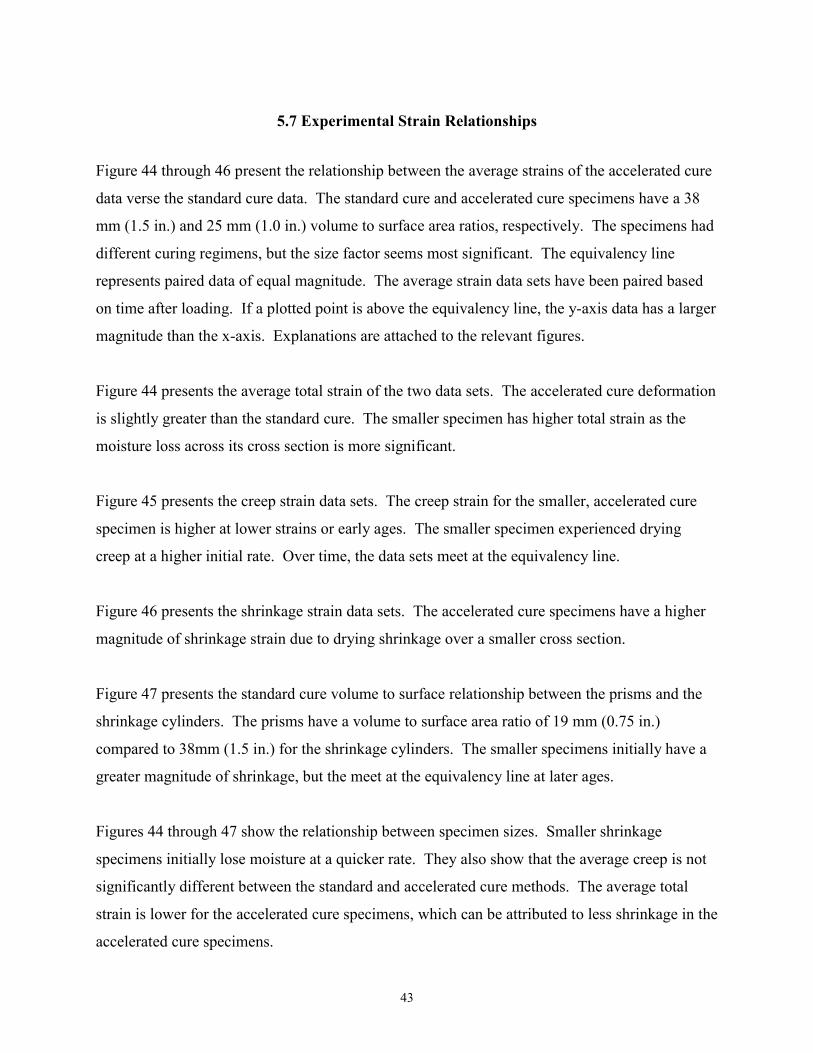
43

5.7 Experimental Strain Relationships

Figure 44 through 46 present the relationship between the average strains of the accelerated cure

data verse the standard cure data. The standard cure and accelerated cure specimens have a 38

mm (1.5 in.) and 25 mm (1.0 in.) volume to surface area ratios, respectively. The specimens had

different curing regimens, but the size factor seems most significant. The equivalency line

represents paired data of equal magnitude. The average strain data sets have been paired based

on time after loading. If a plotted point is above the equivalency line, the y-axis data has a larger

magnitude than the x-axis. Explanations are attached to the relevant figures.

Figure 44 presents the average total strain of the two data sets. The accelerated cure deformation

is slightly greater than the standard cure. The smaller specimen has higher total strain as the

moisture loss across its cross section is more significant.

Figure 45 presents the creep strain data sets. The creep strain for the smaller, accelerated cure

specimen is higher at lower strains or early ages. The smaller specimen experienced drying

creep at a higher initial rate. Over time, the data sets meet at the equivalency line.

Figure 46 presents the shrinkage strain data sets. The accelerated cure specimens have a higher

magnitude of shrinkage strain due to drying shrinkage over a smaller cross section.

Figure 47 presents the standard cure volume to surface relationship between the prisms and the

shrinkage cylinders. The prisms have a volume to surface area ratio of 19 mm (0.75 in.)

compared to 38mm (1.5 in.) for the shrinkage cylinders. The smaller specimens initially have a

greater magnitude of shrinkage, but the meet at the equivalency line at later ages.

Figures 44 through 47 show the relationship between specimen sizes. Smaller shrinkage

specimens initially lose moisture at a quicker rate. They also show that the average creep is not

significantly different between the standard and accelerated cure methods. The average total

strain is lower for the accelerated cure specimens, which can be attributed to less shrinkage in the

accelerated cure specimens.

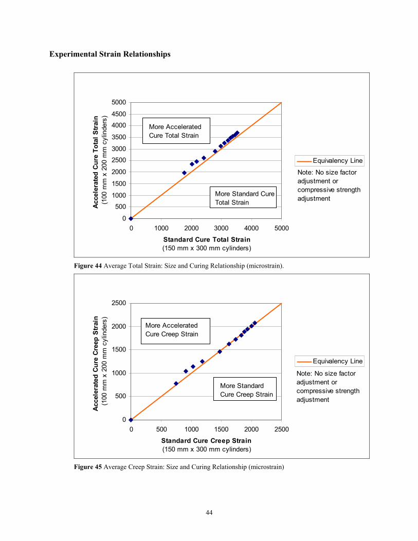
44

Experimental Strain Relationships

0

5001000

1500

2000

25003000

3500

40004500

5000

0 1000 2000 3000 4000 5000

Standard Cure Total Strain (150 mm x 300 mm cylinders)

Acce

lera

ted

Cure

Tot

al S

train

(1

00 m

m x

200

mm

cyl

inde

rs)

Equivalency Line

More Standard Cure Total Strain

More Accelerated Cure Total Strain

Note: No size factor adjustment or compressive strength adjustment

Figure 44 Average Total Strain: Size and Curing Relationship (microstrain).

0

500

1000

1500

2000

2500

0 500 1000 1500 2000 2500

Standard Cure Creep Strain (150 mm x 300 mm cylinders)

Acce

lera

ted

Cure

Cre

ep S

train

(1

00 m

m x

200

mm

cyl

inde

rs)

Equivalency Line

More Standard Cure Creep Strain

More Accelerated Cure Creep Strain

Note: No size factor adjustment or compressive strength adjustment

Figure 45 Average Creep Strain: Size and Curing Relationship (microstrain)

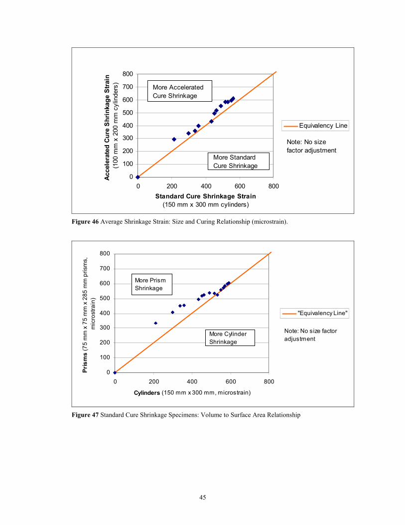
45

0

100

200

300

400

500

600

700

800

0 200 400 600 800Standard Cure Shrinkage Strain

(150 mm x 300 mm cylinders)

Acce

lera

ted

Cure

Shr

inka

ge S

train

(1

00 m

m x

200

mm

cyl

inde

rs)

Equivalency Line

More Standard Cure Shrinkage

Note: No size factor adjustment

More Accelerated Cure Shrinkage

Figure 46 Average Shrinkage Strain: Size and Curing Relationship (microstrain).

0

100

200

300

400

500

600

700

800

0 200 400 600 800

Cylinders (150 mm x 300 mm, microstrain)

Pris

ms

(75

mm

x 7

5 m

m x

285

mm

pris

ms,

m

icro

stra

in)

"Equivalency Line"

More Cylinder Shrinkage

More Prism Shrinkage

Note: No size factor adjustment

Figure 47 Standard Cure Shrinkage Specimens: Volume to Surface Area Relationship

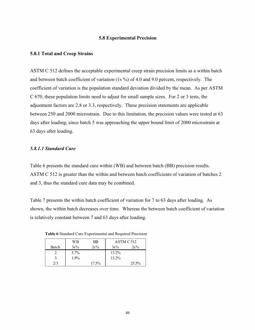
46

5.8 Experimental Precision

5.8.1 Total and Creep Strains

ASTM C 512 defines the acceptable experimental creep strain precision limits as a within batch

and between batch coefficient of variation (1s %) of 4.0 and 9.0 percent, respectively. The

coefficient of variation is the population standard deviation divided by the mean. As per ASTM

C 670, these population limits need to adjust for small sample sizes. For 2 or 3 tests, the

adjustment factors are 2.8 or 3.3, respectively. These precision statements are applicable

between 250 and 2000 microstrain. Due to this limitation, the precision values were tested at 63

days after loading, since batch 5 was approaching the upper bound limit of 2000 microstrain at

63 days after loading.

5.8.1.1 Standard Cure

Table 6 presents the standard cure within (WB) and between batch (BB) precision results.

ASTM C 512 is greater than the within and between batch coefficients of variation of batches 2

and 3, thus the standard cure data may be combined.

Table 7 presents the within batch coefficient of variation for 7 to 63 days after loading. As

shown, the within batch decreases over time. Whereas the between batch coefficient of variation

is relatively constant between 7 and 63 days after loading.

Table 6 Standard Cure Experimental and Required Precision

WB BBBatch 3s% 2s% 3s% 2s%

2 5.7% 13.2%3 1.9% 13.2%

2/3 17.5% 25.5%

ASTM C 512

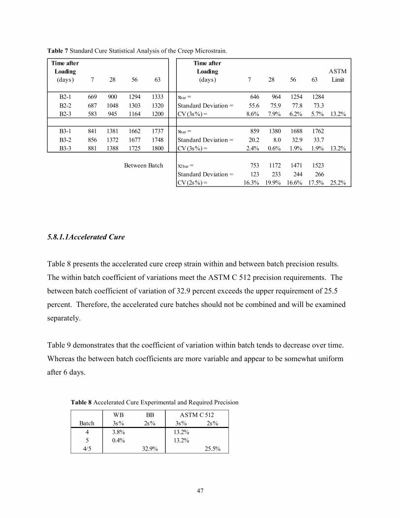
47

Table 7 Standard Cure Statistical Analysis of the Creep Microstrain.

Time afterLoading(days) 7 28 56 63


ASTMLimit

B2-1 669 900 1294 1333 xbar = 646 964 1254 1284B2-2 687 1048 1303 1320 Standard Deviation = 55.6 75.9 77.8 73.3B2-3 583 945 1164 1200 CV (3s%) = 8.6% 7.9% 6.2% 5.7% 13.2%


Between Batch x2bar = 753 1172 1471 1523Standard Deviation = 123 233 244 266CV (2s%) = 16.3% 19.9% 16.6% 17.5% 25.2%

5.8.1.1Accelerated Cure

Table 8 presents the accelerated cure creep strain within and between batch precision results.

The within batch coefficient of variations meet the ASTM C 512 precision requirements. The

between batch coefficient of variation of 32.9 percent exceeds the upper requirement of 25.5

percent. Therefore, the accelerated cure batches should not be combined and will be examined

separately.

Table 9 demonstrates that the coefficient of variation within batch tends to decrease over time.

Whereas the between batch coefficients are more variable and appear to be somewhat uniform

after 6 days.

Table 8 Accelerated Cure Experimental and Required Precision

WB BBBatch 3s% 2s% 3s% 2s%

4 3.8% 13.2%5 0.4% 13.2%

4/5 32.9% 25.5%

ASTM C 512

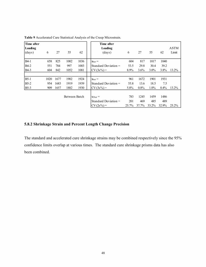
48

Table 9 Accelerated Cure Statistical Analysis of the Creep Microstrain.



ASTMLimit



Between Batch x2bar = 783 1245 1459 1486Standard Deviation = 201 469 485 489CV (2s%) = 25.7% 37.7% 33.2% 32.9% 25.2%

5.8.2 Shrinkage Strain and Percent Length Change Precision

The standard and accelerated cure shrinkage strains may be combined respectively since the 95%

confidence limits overlap at various times. The standard cure shrinkage prisms data has also

been combined.

49

5.9 Prediction Model Residuals

When predicting prestress losses, the most critical information to a designer is to know if a given

model over or under predicts total strain and thus the accompanying prestress losses. The

residuals, the difference between the model and the experimental value, identifies if a model over

predicts, a positive value, and under predicting, a negative value. This identifies if a model is

conservative or unconservative at a given time, but does not identify the best predictor. The

residuals are calculated as the predicted model mean for a batch minus the experimental value

for a test specimen at a given time. The residuals are plotted as the mean and the 95 percent

confidence limits at the given test time. The standard cure residuals are for batches 2 and 3

combined for a total of six test values. Whereas the accelerated cure residuals are for batches 4

and 5 separately. The residuals have been presented in Figures 18 through 39.

Table 6 and 8 summarize the standard and accelerated cure residuals, respectively. The

summary is based on the mean residual being positive or negative. Models that have a residual

of zero or fall within the 95 percent confidence limits are not significant different from the

experimental data and are identified with parentheses (). If a residual could not be distinguished

as positive or negative, then the model is described as good in the chart. A negative residual

means a model under predicted the strain. The accelerated cure values can be positive and

negative since those two batches could not be combined. For the accelerated cure batches,

parentheses () indicate that at least one accelerated cure batch is not significantly different from a

model.

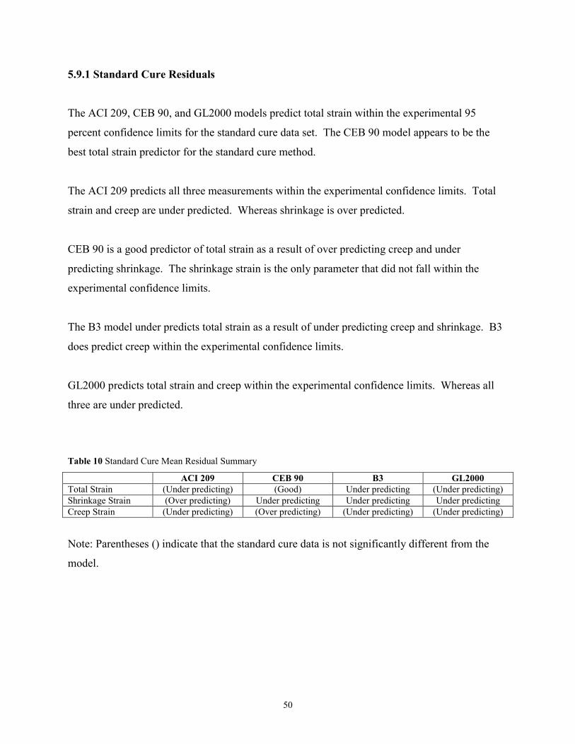
50

5.9.1 Standard Cure Residuals

The ACI 209, CEB 90, and GL2000 models predict total strain within the experimental 95

percent confidence limits for the standard cure data set. The CEB 90 model appears to be the

best total strain predictor for the standard cure method.

The ACI 209 predicts all three measurements within the experimental confidence limits. Total

strain and creep are under predicted. Whereas shrinkage is over predicted.

CEB 90 is a good predictor of total strain as a result of over predicting creep and under

predicting shrinkage. The shrinkage strain is the only parameter that did not fall within the

experimental confidence limits.

The B3 model under predicts total strain as a result of under predicting creep and shrinkage. B3

does predict creep within the experimental confidence limits.

GL2000 predicts total strain and creep within the experimental confidence limits. Whereas all

three are under predicted.

Table 10 Standard Cure Mean Residual Summary

ACI 209 CEB 90 B3 GL2000 Total Strain (Under predicting) (Good) Under predicting (Under predicting) Shrinkage Strain (Over predicting) Under predicting Under predicting Under predicting Creep Strain (Under predicting) (Over predicting) (Under predicting) (Under predicting)

Note: Parentheses () indicate that the standard cure data is not significantly different from the

model.

51

5.9.2 Accelerated Cure Residuals

The best model cannot be identified with residuals when the experimental total strain and creep

data cannot be combined. The residuals do show that the trends to over or under predict strains.

ACI 209 is a good predictor of shrinkage. Whereas the CEB 90, B3, and GL2000 models under

predict shrinkage.

Table 11 Accelerated Cure Residual Summary

ACI 209 CEB 90 B3 GL2000 Total Strain Both over and under Both over and under

predicting Both over and under (Both over and

under predicting) Shrinkage Strain (Good) Under predicting Under predicting Under predicting Creep Strain Both over and under Over predicting Over predicting Over predicting Note: Parentheses () indicate that at least one accelerated cure batch is not significantly different

from the model.

52

5.10 Residuals Squared Analysis

There are numerous methods of analyzing experimental data to determine the best prediction

model. The residuals squared and error percentage methods are considered here, as these have

been shown to be relatively consistent with the other methods (Meyerson). The residuals

squared method puts more weight on larger residuals while preventing residuals of opposite

signs from negating each other. The error percentage is best optimized when using the residuals

from two means. For example, the error percentage can be found between the mean of a

prediction model and a set of data. The error percentage method is not used in this analysis since

the accelerated cure batches cannot be combined according to ASTM C 512. The residuals

squared method identifies the model with the lowest value at a given time as the best predictor.

Residuals Squared = [ ]∑=

6

1

2)(Rei

i at a given time

Tables 12 through 18 present the average residuals so the reader can easily determine if the

model is conservative with a positive residual or unconservative with a negative residual at a

given time.

53

5.10.1 Standard Cure Residuals Squared

Figures 48 through 50 presents the residuals squared for the standard cure specimens. The

rankings will be presented in order with the best first.

The total strain order of best prediction at 56 days is CEB90, GL2000, ACI209, and B3,

respectively. The total strain order of best prediction at 250 days has not changed.

The shrinkage strain order of best prediction at 56 days is ACI 209, GL2000, CEB 90, and B3,

respectively. The shrinkage strain order of best prediction at 250 days remains the same.

The creep strain order of best prediction at 56 days is GL2000, CEB 90, and both the ACI 209

and B3, respectively. The creep strain order of best prediction at 250 days is GL 2000, CEB 90,

B3, and ACI209, respectively.

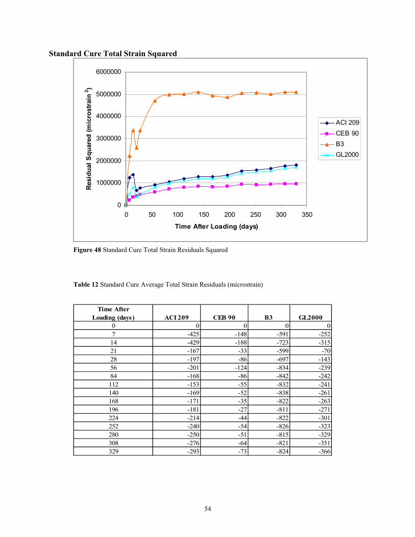
54

Standard Cure Total Strain Squared

0

1000000

2000000

3000000

4000000

5000000

6000000

0 50 100 150 200 250 300 350


Resi

dual

Squ

ared

(mic

rost

rain

2 )

ACI 209CEB 90B3GL2000

Figure 48 Standard Cure Total Strain Residuals Squared

Table 12 Standard Cure Average Total Strain Residuals (microstrain)

Time AfterLoading (days) ACI 209 CEB 90 B3 GL2000

0 0 0 0 07 -425 -148 -591 -25214 -429 -188 -723 -31521 -167 -33 -599 -7028 -197 -86 -697 -14356 -201 -124 -834 -23984 -168 -86 -842 -242112 -153 -55 -832 -241140 -169 -52 -838 -261168 -171 -35 -822 -263196 -181 -27 -811 -271224 -214 -44 -822 -301252 -240 -54 -826 -323280 -250 -51 -815 -329308 -276 -64 -821 -351329 -293 -73 -824 -366

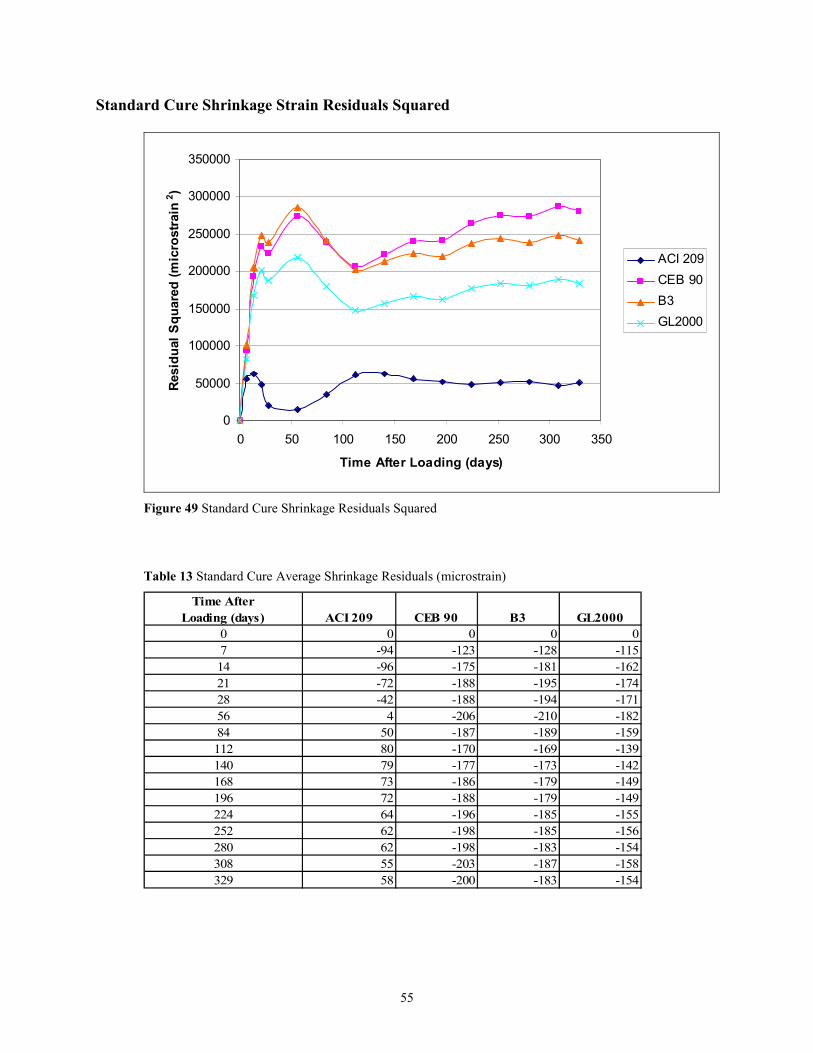
55

Standard Cure Shrinkage Strain Residuals Squared

0

50000

100000

150000

200000

250000

300000

350000

0 50 100 150 200 250 300 350


Resi

dual

Squ

ared

(mic

rost

rain

2 )


Figure 49 Standard Cure Shrinkage Residuals Squared

Table 13 Standard Cure Average Shrinkage Residuals (microstrain)


0 0 0 0 07 -94 -123 -128 -11514 -96 -175 -181 -16221 -72 -188 -195 -17428 -42 -188 -194 -17156 4 -206 -210 -18284 50 -187 -189 -159112 80 -170 -169 -139140 79 -177 -173 -142168 73 -186 -179 -149196 72 -188 -179 -149224 64 -196 -185 -155252 62 -198 -185 -156280 62 -198 -183 -154308 55 -203 -187 -158329 58 -200 -183 -154

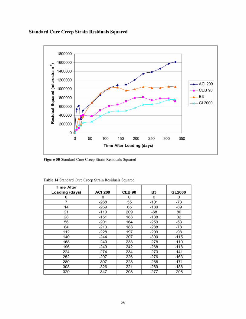
56

Standard Cure Creep Strain Residuals Squared

0

200000

400000

600000

800000

1000000

1200000

1400000

1600000

1800000

0 50 100 150 200 250 300 350


Resi

dual

Squ

ared

(mic

rost

rain

2 )


Figure 50 Standard Cure Creep Strain Residuals Squared

Table 14 Standard Cure Creep Strain Residuals Squared


0 0 0 0 07 -268 55 -101 -7314 -269 65 -180 -8921 -119 209 -68 8028 -151 183 -138 3256 -201 164 -259 -5384 -213 183 -288 -78

112 -228 197 -299 -98140 -244 207 -300 -115168 -240 233 -278 -110196 -249 242 -268 -118224 -274 234 -273 -141252 -297 226 -276 -163280 -307 228 -268 -171308 -326 221 -269 -188329 -347 208 -277 -208

57

5.10.2 Accelerated Cure Residuals Squared

Figures 51 through 53 presents the residuals squared for the accelerated cure specimens. The

rankings will be presented in order with the best first.

The total strain order of best prediction at 56 days is ACI 209, B3, GL2000, and CEB90,

respectively. The total strain order of best prediction at 250 days has not changed.

The shrinkage strain order of best prediction at 56 days is ACI 209, GL2000, CEB 90, and B3,

respectively. The shrinkage strain order of best prediction at 250 days is unchanged.

The creep strain order of best prediction at 56 days is ACI 209, B3, GL2000, and CEB90. The

creep strain order of best prediction at 250 days is unchanged.

5.10.3 Shrinkage Prism Residuals Squared

Figure 54 shows the residuals squared for the shrinkage prisms. The CEB 90 model is initially

the best predictor. At times over 100 days, the B3 model is the best predictor.

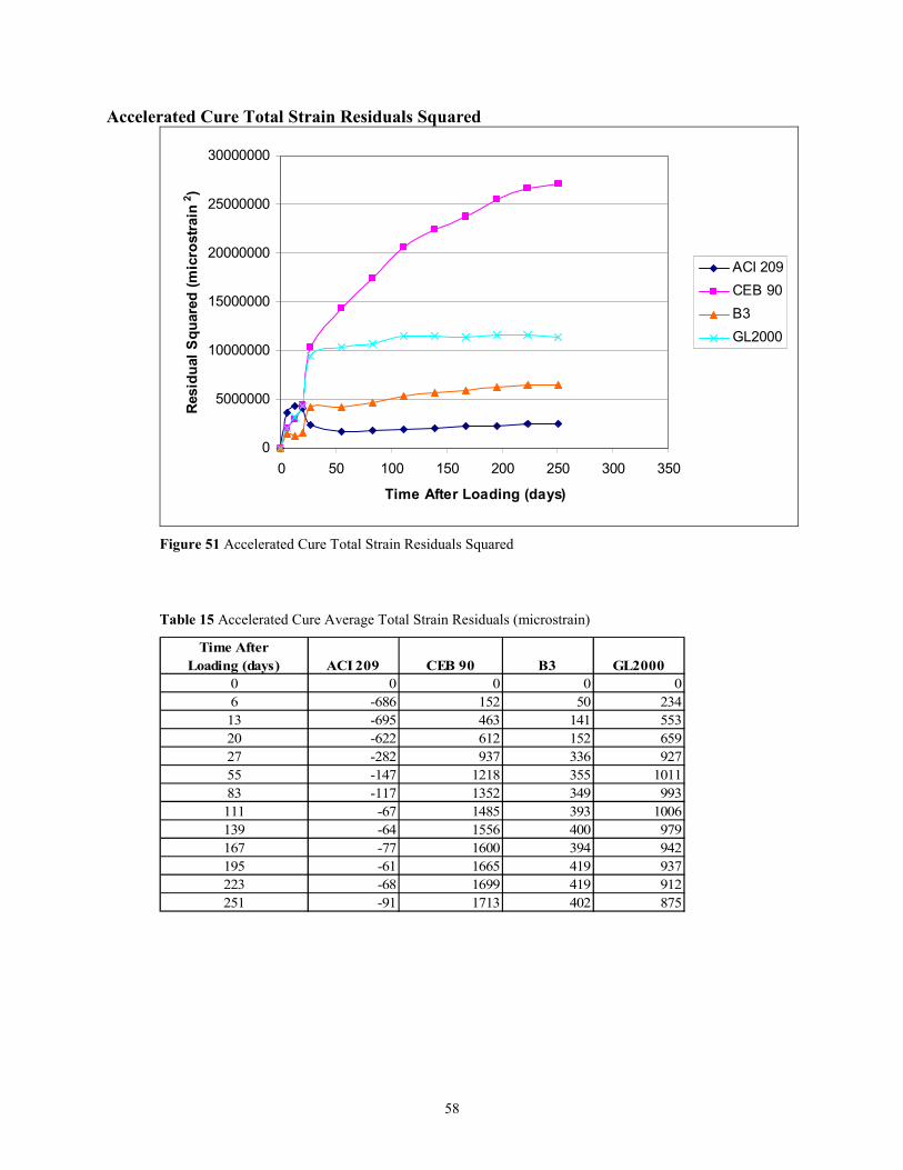
58

Accelerated Cure Total Strain Residuals Squared

0

5000000

10000000

15000000

20000000

25000000

30000000

0 50 100 150 200 250 300 350


Resi

dual

Squ

ared

(mic

rost

rain

2 )


Figure 51 Accelerated Cure Total Strain Residuals Squared

Table 15 Accelerated Cure Average Total Strain Residuals (microstrain)


0 0 0 0 06 -686 152 50 23413 -695 463 141 55320 -622 612 152 65927 -282 937 336 92755 -147 1218 355 101183 -117 1352 349 993111 -67 1485 393 1006139 -64 1556 400 979167 -77 1600 394 942195 -61 1665 419 937223 -68 1699 419 912251 -91 1713 402 875

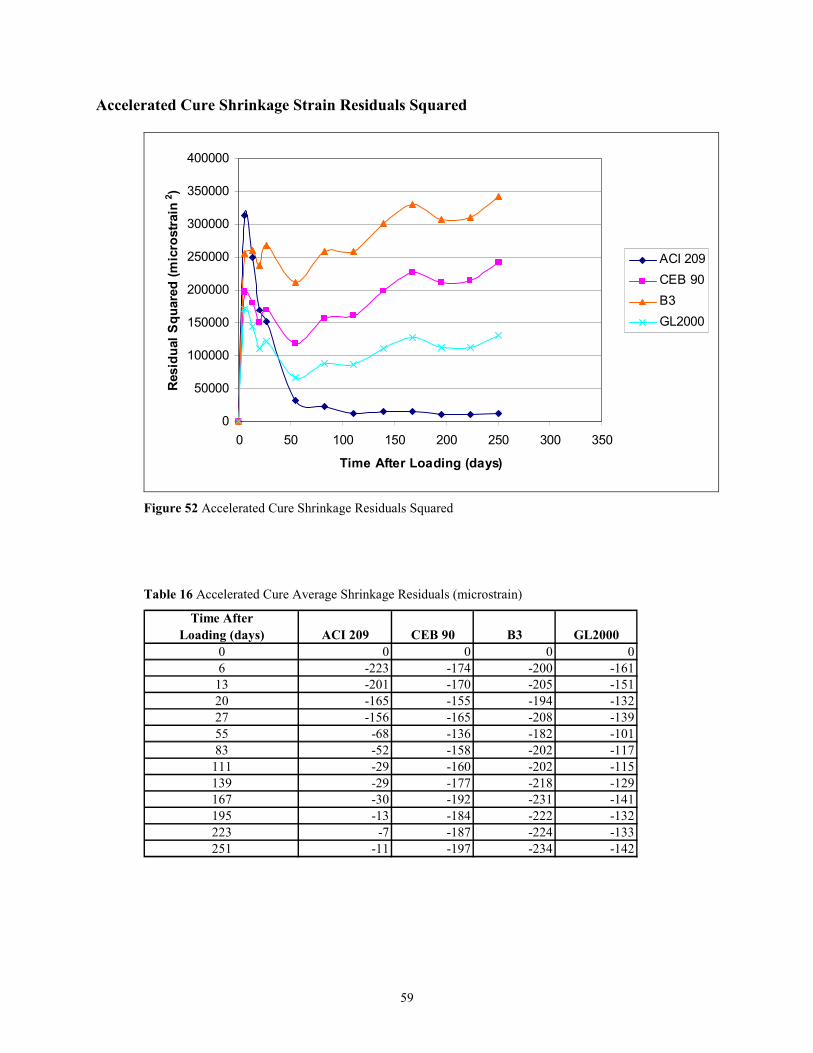
59

Accelerated Cure Shrinkage Strain Residuals Squared

0

50000

100000

150000

200000

250000

300000

350000

400000

0 50 100 150 200 250 300 350


Resi

dual

Squ

ared

(mic

rost

rain

2 )


Figure 52 Accelerated Cure Shrinkage Residuals Squared

Table 16 Accelerated Cure Average Shrinkage Residuals (microstrain)


0 0 0 0 06 -223 -174 -200 -161

13 -201 -170 -205 -15120 -165 -155 -194 -13227 -156 -165 -208 -13955 -68 -136 -182 -10183 -52 -158 -202 -117

111 -29 -160 -202 -115139 -29 -177 -218 -129167 -30 -192 -231 -141195 -13 -184 -222 -132223 -7 -187 -224 -133251 -11 -197 -234 -142

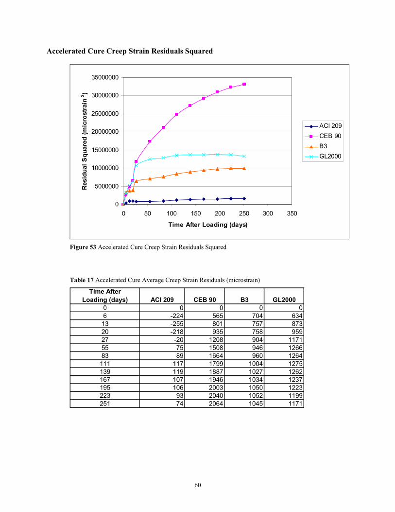
60

Accelerated Cure Creep Strain Residuals Squared

0

5000000

10000000

15000000

20000000

25000000

30000000

35000000

0 50 100 150 200 250 300 350


Resi

dual

Squ

ared

(mic

rost

rain

2 )


Figure 53 Accelerated Cure Creep Strain Residuals Squared

Table 17 Accelerated Cure Average Creep Strain Residuals (microstrain)


0 0 0 0 06 -224 565 704 63413 -255 801 757 87320 -218 935 758 95927 -20 1208 904 117155 75 1508 946 126683 89 1664 960 1264111 117 1799 1004 1275139 119 1887 1027 1262167 107 1946 1034 1237195 106 2003 1050 1223223 93 2040 1052 1199251 74 2064 1045 1171

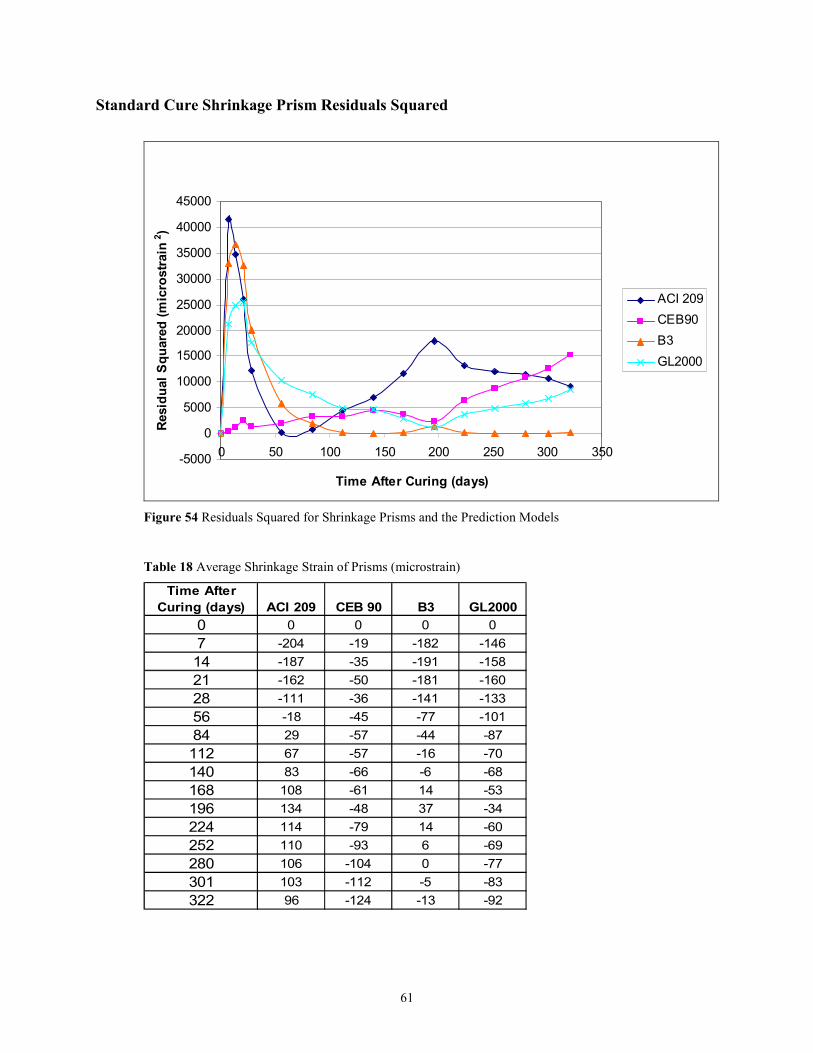
61

Standard Cure Shrinkage Prism Residuals Squared

-5000

0

5000

10000

15000

20000

25000

30000

35000

40000

45000

0 50 100 150 200 250 300 350


Resi

dual

Squ

ared

(mic

rost

rain

2 )

ACI 209CEB90B3GL2000

Figure 54 Residuals Squared for Shrinkage Prisms and the Prediction Models

Table 18 Average Shrinkage Strain of Prisms (microstrain)

Time AfterCuring (days) ACI 209 CEB 90 B3 GL2000

0 0 0 0 07 -204 -19 -182 -14614 -187 -35 -191 -15821 -162 -50 -181 -16028 -111 -36 -141 -13356 -18 -45 -77 -10184 29 -57 -44 -87112 67 -57 -16 -70140 83 -66 -6 -68168 108 -61 14 -53196 134 -48 37 -34224 114 -79 14 -60252 110 -93 6 -69280 106 -104 0 -77301 103 -112 -5 -83322 96 -124 -13 -92

62

5.11 Prediction Model Rankings

This section presents the rankings of the four prediction models. If two or more models were not

significantly different then multiple rankings were assigned. The rankings are summed and the

model with the lowest value is the best overall predictor. If multiple rankings are assigned, the

best ranking is summed.

5.11.1 Standard Cure Rankings

Tables 19 and 20 summarize the standard cure prediction rankings. The GL2000 model is the

best predictor of standard cure time dependent strains. The CEB 90 model is the best predictor

of total strain over time.

Table 19 Standard Cure Prediction Model Rankings at 56 Days

At 56 Days ACI 209 CEB MC 90 B3 GL2000 Total Strain 1/2/3 1/2/3 4 1/2/3 Shrinkage Strain 1 3/4 3/4 2 Creep Strain 3/4 2 3/4 1 Sum of Ranks 5 6 10 4

Table 20 Standard Cure Prediction Model Rankings at 250 Days

At 250 Days ACI 209 CEB MC 90 B3 GL2000 Total Strain 2/3 1 4 2/3 Shrinkage Strain 1 4 3 2 Creep Strain 4 2 3 1 Sum of Ranks 7 7 10 5

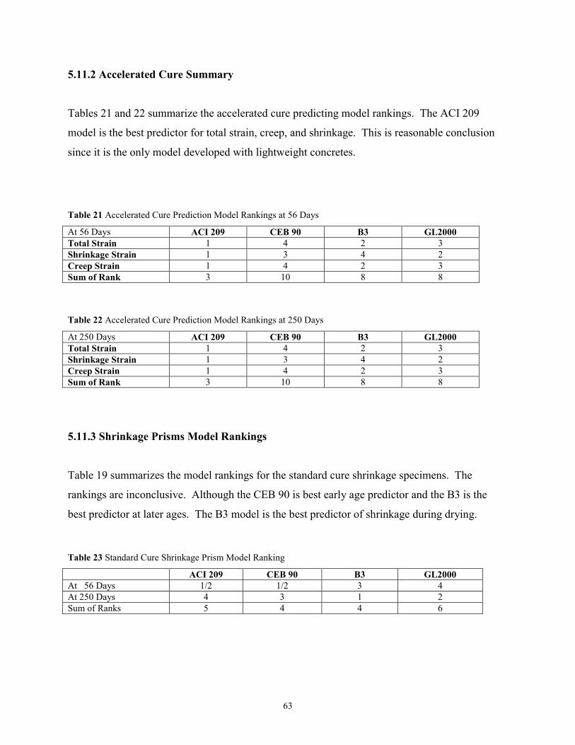
63

5.11.2 Accelerated Cure Summary

Tables 21 and 22 summarize the accelerated cure predicting model rankings. The ACI 209

model is the best predictor for total strain, creep, and shrinkage. This is reasonable conclusion

since it is the only model developed with lightweight concretes.

Table 21 Accelerated Cure Prediction Model Rankings at 56 Days

At 56 Days ACI 209 CEB 90 B3 GL2000 Total Strain 1 4 2 3 Shrinkage Strain 1 3 4 2 Creep Strain 1 4 2 3 Sum of Rank 3 10 8 8 Table 22 Accelerated Cure Prediction Model Rankings at 250 Days

At 250 Days ACI 209 CEB 90 B3 GL2000 Total Strain 1 4 2 3 Shrinkage Strain 1 3 4 2 Creep Strain 1 4 2 3 Sum of Rank 3 10 8 8

5.11.3 Shrinkage Prisms Model Rankings

Table 19 summarizes the model rankings for the standard cure shrinkage specimens. The

rankings are inconclusive. Although the CEB 90 is best early age predictor and the B3 is the

best predictor at later ages. The B3 model is the best predictor of shrinkage during drying.

Table 23 Standard Cure Shrinkage Prism Model Ranking

ACI 209 CEB 90 B3 GL2000 At 56 Days 1/2 1/2 3 4 At 250 Days 4 3 1 2 Sum of Ranks 5 4 4 6

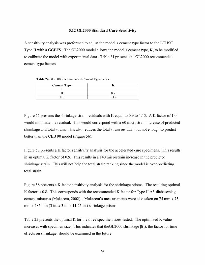
64

5.12 GL2000 Standard Cure Sensitivity

A sensitivity analysis was preformed to adjust the model’s cement type factor to the LTHSC

Type II with a GGBFS. The GL2000 model allows the model’s cement type, K, to be modified

to calibrate the model with experimental data. Table 24 presents the GL2000 recommended

cement type factors.

Table 24 GL2000 Recommended Cement Type factor.

Cement Type K I 1.0 II 0.7 III 1.15

Figure 55 presents the shrinkage strain residuals with K equal to 0.9 to 1.15. A K factor of 1.0

would minimize the residual. This would correspond with a 60 microstrain increase of predicted

shrinkage and total strain. This also reduces the total strain residual, but not enough to predict

better than the CEB 90 model (Figure 56).

Figure 57 presents a K factor sensitivity analysis for the accelerated cure specimens. This results

in an optimal K factor of 0.9. This results in a 140 microstrain increase in the predicted

shrinkage strain. This will not help the total strain ranking since the model is over predicting

total strain.

Figure 58 presents a K factor sensitivity analysis for the shrinkage prisms. The resulting optimal

K factor is 0.8. This corresponds with the recommended K factor for Type II A5-diabase/slag

cement mixtures (Mokarem, 2002). Mokarem’s measurements were also taken on 75 mm x 75

mm x 285 mm (3 in. x 3 in. x 11.25 in.) shrinkage prisms.

Table 25 presents the optimal K for the three specimen sizes tested. The optimized K value

increases with specimen size. This indicates that theGL2000 shrinkage β(t), the factor for time

effects on shrinkage, should be examined in the future.

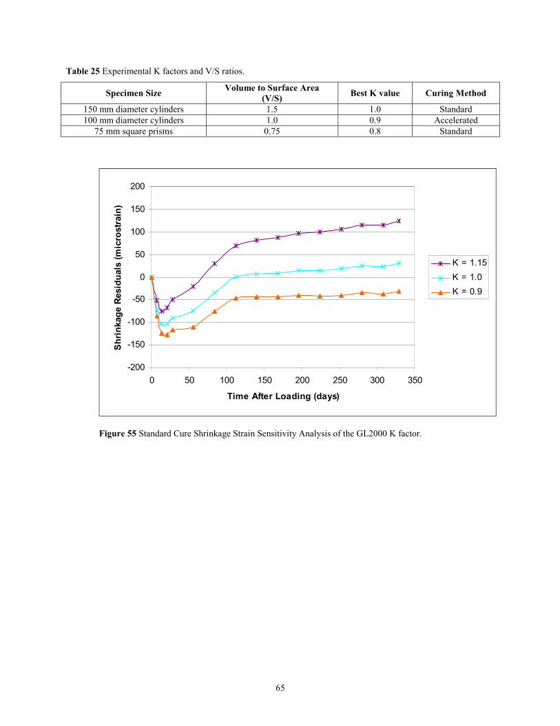
65

Table 25 Experimental K factors and V/S ratios.

Specimen Size Volume to Surface Area (V/S) Best K value Curing Method

150 mm diameter cylinders 1.5 1.0 Standard 100 mm diameter cylinders 1.0 0.9 Accelerated

75 mm square prisms 0.75 0.8 Standard

-200

-150

-100

-50

0

50

100

150

200

0 50 100 150 200 250 300 350


Shrin

kage

Res

idua

ls (m

icro

stra

in)

K = 1.15K = 1.0K = 0.9

Figure 55 Standard Cure Shrinkage Strain Sensitivity Analysis of the GL2000 K factor.

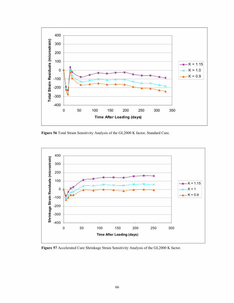
66

-400

-300

-200

-100

0

100

200

300

400

0 50 100 150 200 250 300 350


Tota

l Stra

in R

esid

uals

(mic

rost

rain

)

K = 1.15K = 1.0K = 0.9

Figure 56 Total Strain Sensitivity Analysis of the GL2000 K factor, Standard Cure.

-400

-300

-200

-100

0

100

200

300

400

0 50 100 150 200 250 300


Shrin

kage

Str

ain

Res

idua

ls (m

icro

stra

in)

K = 1.15K = 1K = 0.9

Figure 57 Accelerated Cure Shrinkage Strain Sensitivity Analysis of the GL2000 K factor.

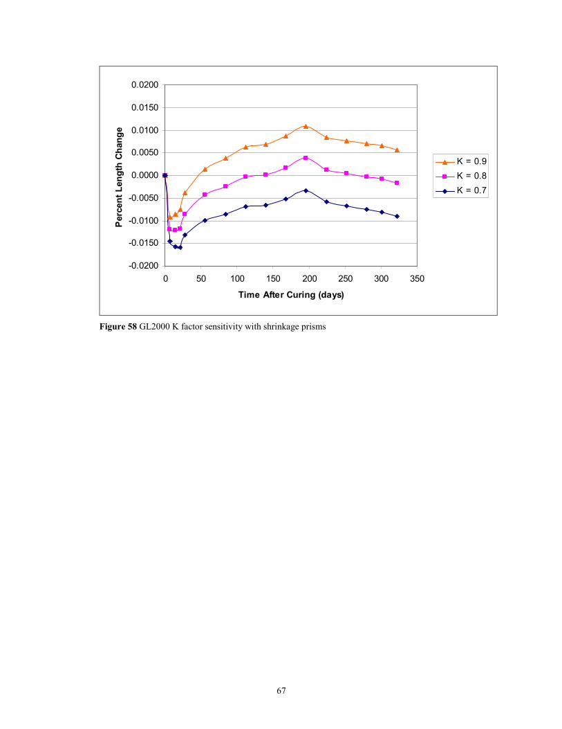
67

-0.0200

-0.0150

-0.0100

-0.0050

0.0000

0.0050

0.0100

0.0150

0.0200

0 50 100 150 200 250 300 350


Perc

ent L

engt

h Ch

ange

K = 0.9K = 0.8K = 0.7

Figure 58 GL2000 K factor sensitivity with shrinkage prisms

68

CHAPTER 6: CONCLUSIONS AND RECOMMENDATIONS

Conclusions

For Accelerated Cure Applications

1. The total strain of the accelerated cure LTHSC batches 4 and 5 were 2510 ± 20

and 3800 ± 160 microstrain at 90 days and 2930 ± 40 and 4470 ± 180 microstrain

at 250 days, respectively, at a five percent significant level.

2. ACI 209 is the best predictor of total strain for the Bayshore LTHSC mixture

when loaded to 40 percent of the ultimate compressive strength and an accelerated

curing method is used.

3. ACI 209 is the best predictor of time dependent deformations.

4. The use of the accelerated cure method significantly increased the variability of

the strength and creep strains. Maturities and unit weights should be kept as

similar as possible.

For Standard Cure Applications

6. The total strain of the standard cure LTHSC mixture was 2970 ± 330 microstrain

at 90 days and 3510 ± 370 microstrain at 250 days at a five percent significant

level.

7. The CEB Mode Code 90 is the best predictor of total strain for the Bayshore

LTHSC mixture when loaded to 40 percent of the ultimate compressive strength

and a standard cure is used.

8. The GL2000 model is the best predictor of time dependent deformations.

69

9. The total strain of Meyerson’s VDOT A5 Limestone GGBFS mixture was

reported as constant at 1470 ± 110 microstrain at 90 days, at a five percent

significant level. This mixture has a shrinkage strain of 350 ± 30 microstrain at

90 days at a five percent significant level. The LTHSC mixture is increasing in

magnitude of both total strain at 2970 ± 330 microstrain and shrinkage strain of

450 ± 60 microstrain at 90 days.

Both mixtures had Grade 120 GGBFS as 40 percent of the cementitious materials.

The water to cementitious materials ratios were 0.33 and 0.37 and the cement

contents were 249 kg/m3 (420 lb/yd3) and 268 kg/m3 (451 lb/yd3) for the A5

mixture and the LTHSC mixture, respectively.

The LTHSC mixture has a significantly larger magnitude of instantaneous and

time dependent deformations. At 90 days after loading, the total strain is twice

that of the VDOT A5 limestone GGBFS mixture and the shrinkage strain is 30

percent greater. Time dependent deformations also continue over a larger period.

Part of this may be attributed to the higher water to cementitious materials ratio

and higher cement paste content of the LTHSC mixture.

70

Recommendations

1. The relationship between laboratory specimens under a constant applied stress and

prestressed beams that have a decreasing applied stress due to prestress losses needs to be

developed or the laboratory testing procedure needs to be modified with a time step

approach.

2. The relationship between the laboratory specimen and bridge beam volume to surface

area ratios should be developed. The study of basic creep and drying creep separately

could be of significance. Laboratory specimens experience a great deal more drying

creep and drying shrinkage than a bridge beam placed over a river.

3. Further examination of the GL2000 model should be conducted with specimens of

various volume to surface area ratios. The equation for shrinkage over time may need

adjusted.

71

References

ACI 213R-87, Guide to Structural Lightweight Aggregate Concrete, ACI Manual of Concrete

Practice, Part 1, 2002.

Mehta, P. K., and Monteiro, P. J. M., Concrete Structure, Properties, and Materials, Second

Edition, Prentice Hall, 1993.

Mokarem, D. W., Development of Concrete Shrinkage Performance Specifications, Doctor of

Philosophy in Civil Engineering, Virginia Tech, May 2002.

Meyerson, R., Compressive Creep of Prestressed Concrete Mixtures with and without Mineral

Admixtures, Master of Science Thesis in Civil Engineering, Virginia Tech, February

2001.

Standard Specifications for Highway Bridges, Adopted and Published by the American

Association of State Highway and Transportation Officials, Inc., sixteenth edition, 1996.

72

APPENDIX A

Literature Review and Prediction Models

73

TABLE OF CONTENTS

INTRODUCTION..................................................................................................................................................... 74

EFFECT OF LTHSC PROPERTIES ON CREEP ................................................................................................ 75

PROPERTIES OF LIGHTWEIGHT CONCRETE .............................................................................................................. 75 VOLUMETRIC CHANGES: INFLUENCES AND MECHANISMS ...................................................................................... 75 CREEP MECHANISMS .............................................................................................................................................. 76 INFLUENCES ON VOLUMETRIC CHANGES ................................................................................................................ 76 AGGREGATE PROPERTIES........................................................................................................................................ 77 EFFECT OF CEMENT TYPE AND FINENESS ............................................................................................................... 78 EFFECT OF CEMENT AND WATER CONTENT............................................................................................................ 78 EFFECT OF CEMENT REPLACEMENT........................................................................................................................ 79 EFFECT OF ADMIXTURES......................................................................................................................................... 79 EFFECT OF CURING ................................................................................................................................................. 79 EFFECT OF ENVIRONMENTAL CONDITIONS ............................................................................................................. 80 EFFECT OF SPECIMEN SIZE ...................................................................................................................................... 80

PRESTRESSED CONCRETE APPLICATIONS OF LIGHTWEIGHT CONCRETE..................................... 81

PREDICTION MODELS......................................................................................................................................... 83

ACI 209R-92 .......................................................................................................................................................... 83 CEB 90 MODEL CODE ............................................................................................................................................ 84 B3 MODEL .............................................................................................................................................................. 84 GL2000 .................................................................................................................................................................. 85 SAK........................................................................................................................................................................ 85

MODEL LIMITATIONS AND REQUIRED PARAMETERS ............................................................................ 87

SUMMARY OF PREDICTION MODEL NOMENCLATURE AND EQUATIONS ........................................ 89

ACI 209 CODE MODEL ........................................................................................................................................... 89 CEB 90 CODE MODEL ............................................................................................................................................ 94 THE B3 MODEL....................................................................................................................................................... 99 THE GL2000 MODEL ............................................................................................................................................ 104 THE SAK MODEL ................................................................................................................................................. 108

REFERENCES........................................................................................................................................................ 110

74

INTRODUCTION

Concrete undergoes volumetric changes throughout its service life. These changes are a result of




The summation of instantaneous and time dependent deformations is called total deformation.

Shrinkage is a combination of autogeneous, drying, and carbonation shrinkage of the hardened

concrete. Plastic shrinkage is not included since it occurs due to moisture loss before the

concrete has set. Autogeneous shrinkage is a result of the hydration process. The hydrated

cement paste has a smaller volume than the cement and water reactants. Drying shrinkage

occurs as surface water evaporates and internal water moves outward in an attempt for hygral

equilibrium. The opposite reaction is called swelling. Carbonation shrinkage occurs with the

carbonation of the hydrated cement products with carbon dioxide in the atmosphere.

Creep testing is conducted on sealed or unsealed specimens. Sealed specimens with an applied

stress have volumetric changes due to elastic deformation, basic creep, and autogeneous

shrinkage. Sealed specimens without an applied stress deform due to autogeneous shrinkage.

Basic creep is the total deformation of a loaded, sealed specimen minus the elastic deformation

and autogeneous shrinkage.

Unsealed specimens are the most commonly used test method. Unsealed specimens without an

applied stress have volumetric changes due to autogeneous and drying shrinkage. The total

deformation of unsealed specimens is the result of an applied stress producing an elastic

deformation, creep, and shrinkage. Creep includes both basic and drying creep. Shrinkage

includes autogeneous and drying shrinkage. Drying creep of a loaded specimen is the total

deformation minus the elastic deformation, basic creep, and autogeneous shrinkage and requires

the testing of both sealed and unsealed specimens. Therefore, creep is typically examined as the

total of basic and drying creep.

75

EFFECT OF LTHSC PROPERTIES ON CREEP

Properties of Lightweight Concrete

Lightweight aggregates are weaker than normal weight aggregates so higher cement contents are

needed to get a required strength for a mixture. This increases the amount of cement paste,

which will lead to increased creep (Clarke). This decrease in stiffness can be seen in modulus of

elasticity measurements of lightweight concretes (Nawy).

Lightweight aggregates have relatively large pore volumes, which makes water absorption more

important than with denser normal weight aggregates (Clarke). The water to cement ratio and

slump can be impacted more significantly with changes in aggregate moisture conditions if water

content is not adjusted. Workability can decrease between mixing and placing as moisture is

absorbed by lightweight aggregates (Clarke). Possible segregation of the mix should be

considered since lightweight aggregates can begin to float when larger slumps are used.

Volumetric Changes: Influences and Mechanisms

The two types of volumetric changes examined are drying shrinkage and creep. Drying

shrinkage is the decrease in volume of hardened concrete with time due to the loss of moisture,

while excluding thermal effects. Creep is the time dependent deformations due to a sustained

stress. The term “creep” refers to both drying and basic creep, which occur with and without

moisture loss respectively. Neville and Gilbert prefer to identify creep as the time-dependent

deformation in excess of shrinkage.

The following are other types of volumetric changes. Plastic shrinkage occurs before the

concrete sets. Carbonation shrinkage is a result to the hardened cement paste reacting with

carbon dioxide in the atmosphere. Autogeneous shrinkage is due to drying as the cement paste

hardens during hydration.

76

Creep Mechanisms

The literature considers many mechanisms as the theoretical basis of creep. Gilbert states no

single theory accounts for all of the phenomena and that all of the following four mechanisms

contribute. Viscous flow occurs from sliding of the colloidal sheets in the cement gel between

absorbed water. Seepage or the expulsion and decomposition of the interlayer water within the

cement gel. Delayed elasticity or the time dependent elastic deformation between the aggregate

and gel crystals as viscous flow and seepage occur within the cement gel. Gilbert also notes the

at high stress levels, the additional deformation can occur and the transition zone breaks down.

Mehta describes creep and drying shrinkage as the removal of adsorbed water from the hydrated

cement paste. Drying shrinkage is caused by the loss of physically adsorbed water from the C-S-

H that causes a shrinkage strain. The differential relative humidity or an applied load act as the

driving force to create a hydrostatic tension in the small capillaries (< 50nm) of the hydrated

cement paste. Mehta states that loads above 30 to 40 percent of the compressive strength lead to

microcracking in the transition zone. Delayed elastic deformation also occurs as loads are

transferred back and form between the aggregate and the cement paste as they each deform

elastically over time.

Influences on Volumetric Changes

Lightweight, high strength concrete has many influences on its volumetric changes. These

involve aggregate properties, cement type and fineness, cement and water content, cement

replacements, admixtures, curing, environmental conditions, and specimen size.

77

Aggregate Properties

Aggregate strength is generally overlooked since normal weight aggregate is typically several

times stronger than the cement paste and transition zone. Lightweight aggregate is an exception

(Metha). Aggregates properties are critical to the amount of creep, since the aggregates have a

restraining affect on the magnitude of creep (Neville). Mokarem noted that diabase aggregate

mixtures experienced greater drying shrinkage than limestone and gravel mixtures.

The ACI 213 Guide for Structural Lightweight Aggregate Concrete discusses how the high

magnitude and variation in lightweight aggregate absorption and absorption rates can

significantly differ mixture proportions with that of normal weight mixtures. This results in

significantly different water and cement contents. Lightweight aggregates typically absorb 5 to

twenty percent by weight of the drying aggregate. If the lightweight aggregates are not

presoaked then the aggregate can pull moisture out of the fresh mix resulting in a loss in

workability. Additional strength can be gained by presoaking the aggregate for 24 hours before

mixing. The excess moisture in the lightweight aggregate will internally prolong the curing

process.

Aggregates have a large role in determining the modulus of elasticity of a concrete mix.

Influential aggregate properties are porosity, maximum size, shape, surface texture, grading, and

mineralogical composition. Mehta states with lightweight concrete, the modulus of elasticity of

the aggregate is the most important.

As the load is transferred to the aggregate, the creep and drying shrinkage of the cement paste is

partially restrained. Therefore, concretes with high aggregate contents are less vulnerable to

high creep or shrinkage strains (Nawy). Nawy also notes research has shown that smaller

aggregates, 9.5 mm (3/8 in.) maximum can increase the compressive strength from 44.8 MPa

(6,500 psi) to over 55 MPa (8,000 psi). Smaller aggregate sizes are also known to increase creep

and shrinkage.

78

The "ceiling" strength of a concrete depends on the aggregate type (Clarke). The "ceiling" is

reached when the capacity of the cement paste and transition zone is reached and the concrete

can no longer transfer load to the aggregate.

Effect of Cement Type and Fineness

The cement is the most important factor since creep occurs in the hydrated cement paste. It

affects creep in two ways: the physical and chemical properties (Neville). The physical and

chemical properties have a direct affect on the strength of the cement paste. The physical

properties relate to fineness, which has a direct relationship with the rate of hydration. The

smaller the cement particles, the faster they are going to hydrate and gain strength. There is not a

direct relationship between chemical composition and creep, but there is relationship between

chemical composition of the cement and strength. The finer the cement the more C3A that is

available at early ages, which results higher rate of strength gain (Neville). Higher strength

normal weight concretes typically creep and shrinkage less.

Effect of Cement and Water Content

The quantity of cement paste is important due to aggregate having a restraining affect on the

magnitude of creep (Neville). As cement content increases, the influence of the aggregates

decrease as the mixture is being diluted with cement paste. For lightweight concrete, cement

content is a good indication of strength for mix design purposes (Clarke). The compressive

strength of a LTHSC mixture is usually rated to the cement content at a given slump than the

water to cement ratio (ACI 213)

Lower water contents result in lower creep and shrinkage strains. A more dense cement paste

will strain less. The variability of the absorption properties of lightweight aggregates have a

direct relationship on the between batch consistency of water to cement ratios (ACI 213).

79

Effect of Cement Replacement

Cement replacements include ground granulated blast furnace slag(GGBFS), fly ash, and silica

fume. An increase in creep will occur when GGBFS or other pozzolan material is used as a

partial cement replacement for Type I cement (Mehta). Silica fume will increase the hydration

rate with its particle size of one-hundreth that of a cement particle. Silica fume will increase

shrinkage. Mehta states that pozzolans tend to increase the volume of fine pores (3 to 20 nm)

which increases creep and shrinkage. Although, Nawy says pozzolans help fill the matrix voids

which creates a denser matrix and stronger mix.

Effect of Admixtures

Cabrera et al found that superplasticizers that reduce the surface tension of water also increase

creep and shrinkage strains in cement paste. This is being attributed to a larger volume of total

pores and a courser size distribution, a larger negative pore pressure at constant humidity, and a

lower degree of saturation at a constant humidity.

Concrete with entrained air would creeps more, but entrainment agents reduce the required

water. This reduction in water compensates for the increased air voids (Neville).

Using calcium chloride or triethanolamine as an accelerator also increases creep and shrinkage

(Mehta, Neville).

Effect of Curing

Moist curing allows concrete to continue hydration without being limited by the availability for

water. Dry cured concrete specimens are dependent on the internal moisture for hydration. A

dry cured specimen will have less creep potential due to less moisture being present in the paste

(Neville). Lightweight aggregate concretes are more tolerant of poor curing conditions since the

aggregate has a larger water reserve in the poor system (Nawy).

80

Effect of Environmental Conditions

Muller compared specimens of various thicknesses to both constant and cyclic humidity

conditions. They found that cyclic humidity increases creep, but does not increase shrinkage

(Mehta, Muller, Neville). If the concrete dries, then hydration will slow along with any strength

increase (Neville, Clarke).

Muller also notes that Bazant’s models are the only ones that take cyclic ambient conditions into

consideration. The ACI 209, CEB90 and B3 consider the environmentally temperature in the

prediction models.

Effect of Specimen Size

The specimen size factor is significant to drying creep and drying shrinkage since they are a

function of water removal (Mehta). It is typically a function of the volume to surface area since

it relates the distance water must travel to leave a specimen. The ratio of volume to surface area

is also called the theoretical thickness (Mehta). An increase in the thickness of a member will

result in a decrease in the members creep strain (Nawy).

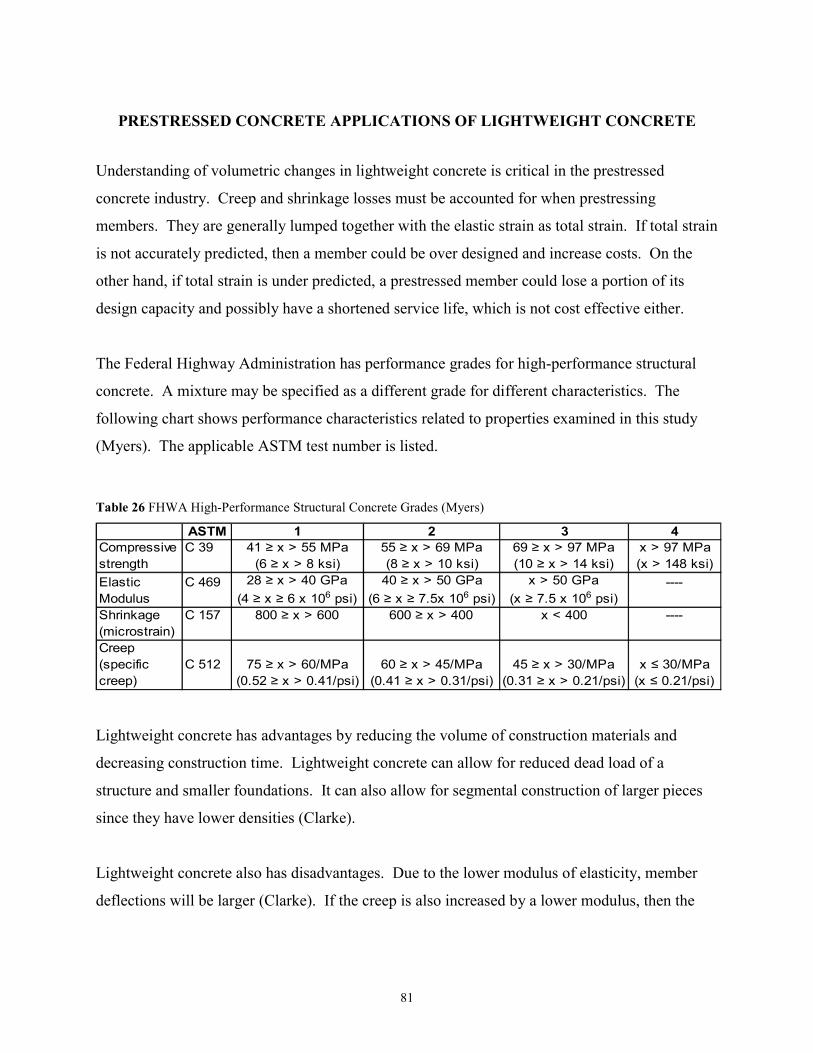
81

PRESTRESSED CONCRETE APPLICATIONS OF LIGHTWEIGHT CONCRETE

Understanding of volumetric changes in lightweight concrete is critical in the prestressed

concrete industry. Creep and shrinkage losses must be accounted for when prestressing

members. They are generally lumped together with the elastic strain as total strain. If total strain

is not accurately predicted, then a member could be over designed and increase costs. On the

other hand, if total strain is under predicted, a prestressed member could lose a portion of its

design capacity and possibly have a shortened service life, which is not cost effective either.

The Federal Highway Administration has performance grades for high-performance structural

concrete. A mixture may be specified as a different grade for different characteristics. The

following chart shows performance characteristics related to properties examined in this study

(Myers). The applicable ASTM test number is listed.

Table 26 FHWA High-Performance Structural Concrete Grades (Myers)

ASTM 1 2 3 4Compressive strength

C 39 41 ≥ x > 55 MPa(6 ≥ x > 8 ksi)

55 ≥ x > 69 MPa(8 ≥ x > 10 ksi)

69 ≥ x > 97 MPa(10 ≥ x > 14 ksi)

x > 97 MPa(x > 148 ksi)

Elastic Modulus

C 469 28 ≥ x > 40 GPa(4 ≥ x ≥ 6 x 106 psi)

40 ≥ x > 50 GPa(6 ≥ x ≥ 7.5x 106 psi)

x > 50 GPa(x ≥ 7.5 x 106 psi)

----

Shrinkage(microstrain)

C 157 800 ≥ x > 600 600 ≥ x > 400 x < 400 ----

Creep(specific creep)

C 512 75 ≥ x > 60/MPa(0.52 ≥ x > 0.41/psi)

60 ≥ x > 45/MPa(0.41 ≥ x > 0.31/psi)

45 ≥ x > 30/MPa(0.31 ≥ x > 0.21/psi)

x ≤ 30/MPa(x ≤ 0.21/psi)

Lightweight concrete has advantages by reducing the volume of construction materials and

decreasing construction time. Lightweight concrete can allow for reduced dead load of a

structure and smaller foundations. It can also allow for segmental construction of larger pieces

since they have lower densities (Clarke).

Lightweight concrete also has disadvantages. Due to the lower modulus of elasticity, member

deflections will be larger (Clarke). If the creep is also increased by a lower modulus, then the

82

member will camber upward more than predicted. Lightweight aggregates, like expanded slate,

are manmade so they are more expensive than natural aggregates.

83

PREDICTION MODELS

Five prediction models for creep and shrinkage are examined. The ACI 209 model is

recommended by the American Concrete Institute. The CEB-FIP Mode Code 90 is used in

Europe. Other models include the B3, which was developed by Bazant, the GL model, which

was developed by Gardner, and the SAK model, which was developed by Sakata.

The models look at free shrinkage, creep strain, and elastic deformation. Free shrinkage is the

combination of all shrinkage strains without an applied load. The creep strain is the combination

of the basic and drying creep. The elastic deformation is the instantaneous recoverable

deformation of a concrete specimen during the loading process.

The various creep models relate the creep strain to the loading conditions by using creep

coefficient, specific creep, or creep compliance. The creep coefficient is the ratio of creep strain

at given time to the initial elastic strain. Specific creep is the creep strain per unit stress. The

creep compliance is the ratio of creep strain plus elastic strain per unit stress.

ACI 209R-92

The ACI 209 model was developed by the American Concrete Institute and is used in the

AASHTO LRFD method. The ACI 209 Model was created from data that included normal

weight, sand lightweight, and lightweight concrete while also incorporating Type I and III

cement and moist and steam curing. It was found that there was no significant difference

between different weight concretes for creep and shrinkage. The code notes that more consistent

results were found by using the creep coefficient or the ratio of creep strain to initial strain. This

was due to the initial stiffness of the concrete being accounted for.

The code allows for the following variation to the standard conditions: concrete composition, age

at loading, ambient relative humidity, size factor, and ambient temperature. The concrete

composition correction factors apply to slump, fine aggregate percentage, cement content, and

air content. Either the average thickness method or the volume to surface ratio method can

84

adjust the size factor. The volume to surface area ratio was used since it is more applicable to

prestressed concrete beams.

CEB 90 Model Code

The CEB Model Code 90 is the European design code recommended by the Euro-International

Concrete Committee and International Federation for Prestressing). This model was preceded by

the CEB-FIP 1970 model and the CEB-FIP 1978 model. The CEB-FIP 1970 model was a

product model that adjusted for mix properties and environmental conditions with multiplication

factors from graphs. The CEB-FIP 1978 model was a summation model that had corrections

factors that needed to be summed from graphs.

The CEB MC 90 is a product prediction model, which is designed to predict the mean time

dependent deformation for normal weight, plane structural concrete. It only takes into account

parameters that are generally known to the designer in the design stage. The CEB model has a

coefficient of variation of 20.4% and 32.9% for creep compliance and shrinkage respectively.

The following parameters are required to predict the creep coefficient: mean or design strength

of the concrete, member dimensions, mean relative humidity of the ambient atmosphere, age at

loading, and duration of loading. In addition to these parameters, the cement type is needed to

predict shrinkage strain.

B3 Model

The B3 model is the creation of Z. P. Bazant and S. Baweja. Earlier versions of the model were

the BP model in 1978 and the BP-KX model in 1991. The BP-KX has an expanded and a short

form. The expanded form is for structures highly sensitive to creep and shrinkage. The short

form predicted creep compliance in a design code method. The B3 model is design to meet the

requirements of the RILEM TC 107 for a simpler model.

85

The B3 model can be applied to concretes outside of the limitations if the parameters are

calibrated with tests.

GL2000

N. J. Gardner and M. J. Lockman developed the GL2000 Model as a design office procedure to

predict creep and shrinkage. Gardner and J. W. Zhao’s GZ Model from 1993 preceded this

product model.

The predicted values can be improved by measuring the compressive strength and modulus of

elasticity. This model uses the modulus of elasticity and compressive strength measurements to

adjust for aggregate stiffness. Aggregate stiffness is a factor in elastic deformation, creep, and

shrinkage. The GL2000 model uses the experimental modulus to have a compressive strength

back calculated from it. This value is averaged with the compressive strength and an adjusted

modulus is calculated. The creep coefficient prediction uses the time at loading, time at the

beginning of shrinkage, volume to surface area ratio, and the ambient relative humidity. The

model has a factor, Ф(tc), to adjust for moisture loss before loading. If the time of loading is

equal to the time at the beginning of shrinkage, then Ф(tc) equals one. The specific creep is

found by dividing the creep coefficient by the adjusted modulus of elasticity. The instantaneous

elastic strain can be found by dividing the applied load by the modulus of elasticity at the time of

loading. Shrinkage strain is predicted with correction factors for the effect of cement type on

shrinkage, the effect of time on shrinkage using the volume to surface ratio, and humidity. The

ultimate shrinkage strain is a function of the mean 28-day compressive strength.

SAK

The SAK was developed by K. Sakata and is the recommended method of Japan Society of Civil

Engineers. The model separately predicts ultimate values of drying creep, basic creep, and

shrinkage. Water and cement content are used in predicting both drying and basic creep. The

ambient relative humidity is used with the volume to surface area of the member to predict both

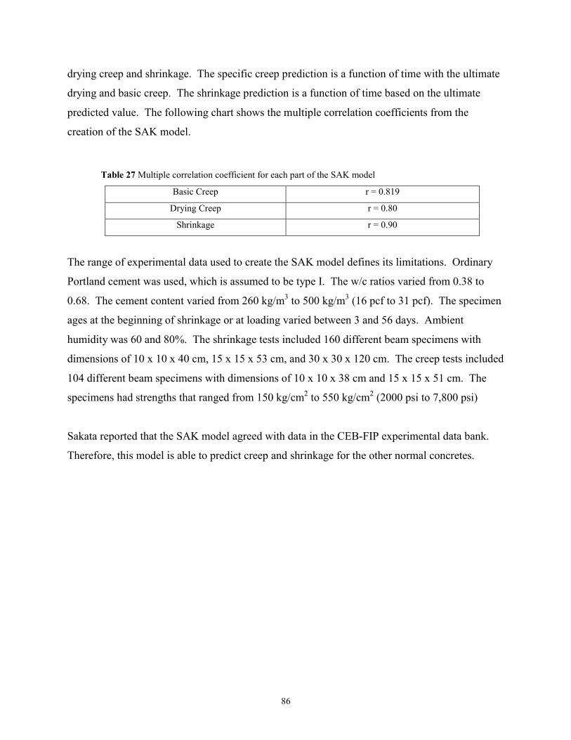
86

drying creep and shrinkage. The specific creep prediction is a function of time with the ultimate

drying and basic creep. The shrinkage prediction is a function of time based on the ultimate

predicted value. The following chart shows the multiple correlation coefficients from the

creation of the SAK model.

Table 27 Multiple correlation coefficient for each part of the SAK model

Basic Creep r = 0.819

Drying Creep r = 0.80

Shrinkage r = 0.90

The range of experimental data used to create the SAK model defines its limitations. Ordinary

Portland cement was used, which is assumed to be type I. The w/c ratios varied from 0.38 to

0.68. The cement content varied from 260 kg/m3 to 500 kg/m3 (16 pcf to 31 pcf). The specimen

ages at the beginning of shrinkage or at loading varied between 3 and 56 days. Ambient

humidity was 60 and 80%. The shrinkage tests included 160 different beam specimens with

dimensions of 10 x 10 x 40 cm, 15 x 15 x 53 cm, and 30 x 30 x 120 cm. The creep tests included

104 different beam specimens with dimensions of 10 x 10 x 38 cm and 15 x 15 x 51 cm. The

specimens had strengths that ranged from 150 kg/cm2 to 550 kg/cm2 (2000 psi to 7,800 psi)

Sakata reported that the SAK model agreed with data in the CEB-FIP experimental data bank.

Therefore, this model is able to predict creep and shrinkage for the other normal concretes.

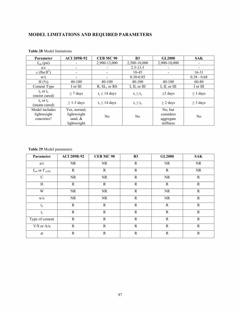
87

MODEL LIMITATIONS AND REQUIRED PARAMETERS

Table 28 Model limitations

Parameter ACI 209R-92 CEB MC 90 B3 GL2000 SAK fcm (psi) - 2,900-13,000 2,500-10,000 2,900-10,000 -

a/c - - 2.5-13.5 - - c (lbs/ft3) - - 10-45 - 16-31

w/c - - 0.30-0.85 0.38 - 0.68 H (%) 40-100 40-100 40-100 40-100 60-80

Cement Type I or III R, SL, or RS I, II, or III I, II, or III I or III to or ts

(moist cured) ≥ 7 days ts ≤ 14 days ts ≤ to ≥2 days ≥ 3 days

to or ts (steam cured) ≥ 1-3 days ts ≤ 14 days ts ≤ to ≥ 2 days ≥ 3 days

Model includes lightweight concretes?

Yes, normal, lightweight

sand, & lightweight

No No

No, but considers aggregate stiffness

No

Table 29 Model parameters

Parameter ACI 209R-92 CEB MC 90 B3 GL2000 SAK

a/c NR NR R NR NR

fcm or f’c(28) R R R R NR

C NR NR R NR R

H R R R R R

W NR NR R NR R

w/c NR NR R NR R

to R R R R R

ts R R R R R

Type of cement R R R R R

V/S or A/u R R R R R

σ

R R R R R

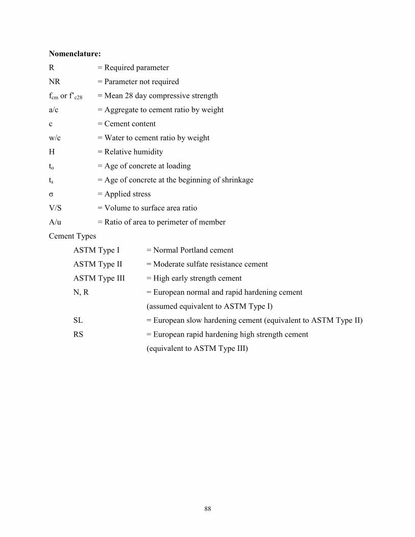
88

Nomenclature:

R = Required parameter

NR = Parameter not required

fcm or f’c28 = Mean 28 day compressive strength

a/c = Aggregate to cement ratio by weight

c = Cement content

w/c = Water to cement ratio by weight

H = Relative humidity

to = Age of concrete at loading

ts = Age of concrete at the beginning of shrinkage

σ = Applied stress

V/S = Volume to surface area ratio

A/u = Ratio of area to perimeter of member

Cement Types

ASTM Type I = Normal Portland cement

ASTM Type II = Moderate sulfate resistance cement

ASTM Type III = High early strength cement

N, R = European normal and rapid hardening cement

(assumed equivalent to ASTM Type I)

SL = European slow hardening cement (equivalent to ASTM Type II)

RS = European rapid hardening high strength cement

(equivalent to ASTM Type III)

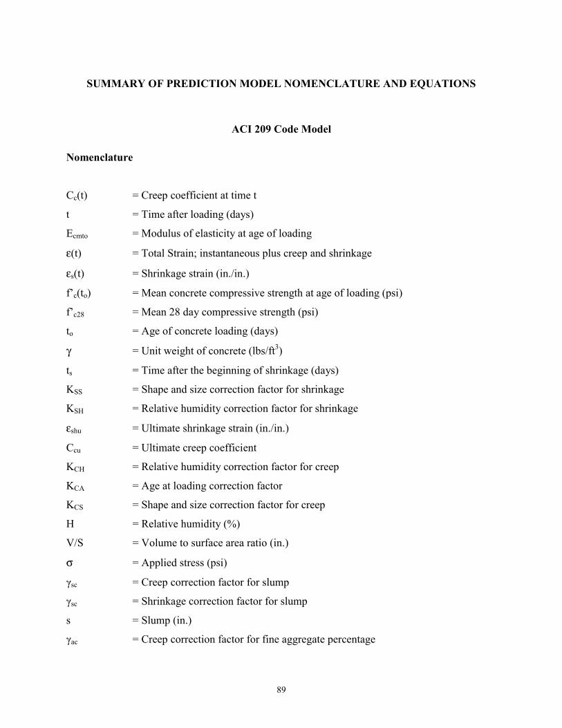
89

SUMMARY OF PREDICTION MODEL NOMENCLATURE AND EQUATIONS

ACI 209 Code Model

Nomenclature

Cc(t) = Creep coefficient at time t

t = Time after loading (days)

Ecmto = Modulus of elasticity at age of loading

ε(t) = Total Strain; instantaneous plus creep and shrinkage

εs(t) = Shrinkage strain (in./in.)

f’c(to) = Mean concrete compressive strength at age of loading (psi)

f’c28 = Mean 28 day compressive strength (psi)

to = Age of concrete loading (days)

γ = Unit weight of concrete (lbs/ft3)

ts = Time after the beginning of shrinkage (days)

KSS = Shape and size correction factor for shrinkage

KSH = Relative humidity correction factor for shrinkage

εshu = Ultimate shrinkage strain (in./in.)

Ccu = Ultimate creep coefficient

KCH = Relative humidity correction factor for creep

KCA = Age at loading correction factor

KCS = Shape and size correction factor for creep

H = Relative humidity (%)

V/S = Volume to surface area ratio (in.)

σ = Applied stress (psi)

γsc = Creep correction factor for slump

γsc = Shrinkage correction factor for slump

s = Slump (in.)

γac = Creep correction factor for fine aggregate percentage

90

γas = Shrinkage correction factor for fine aggregate percentage

ψ = Fine aggregate percentage (%)

γαc = Creep correction factor for air content

γαs = Shrinkage correction factor for air content

α = Air content (%)

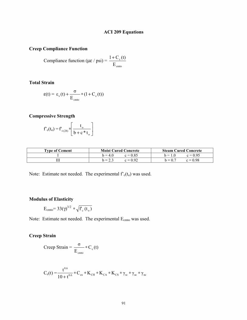
91

ACI 209 Equations

Creep Compliance Function

Compliance function (µε / psi) = cmto

c

E(t)C1+

Total Strain

ε(t) = )(t)C1(Eσ(t)ε ccmto

s +∗+

Compressive Strength

f’c(to) =

+∗

o

o(28)c t*cb

tf'

Type of Cement Moist Cured Concrete Steam Cured Concrete

I b = 4.0 c = 0.85 b = 1.0 c = 0.95 III b = 2.3 c = 0.92 b = 0.7 c = 0.98

Note: Estimate not needed. The experimental f’c(to) was used.

Modulus of Elasticity

Ecmto= 33(γ)3/2 )(tf' oc∗

Note: Estimate not needed. The experimental Ecmto was used.

Creep Strain

Creep Strain = (t)CEσ

ccmto

∗

Cc(t) = αcacscCSCACHcu0.6

0.6

γγγK K K Ct10

t ∗∗∗∗∗∗∗+

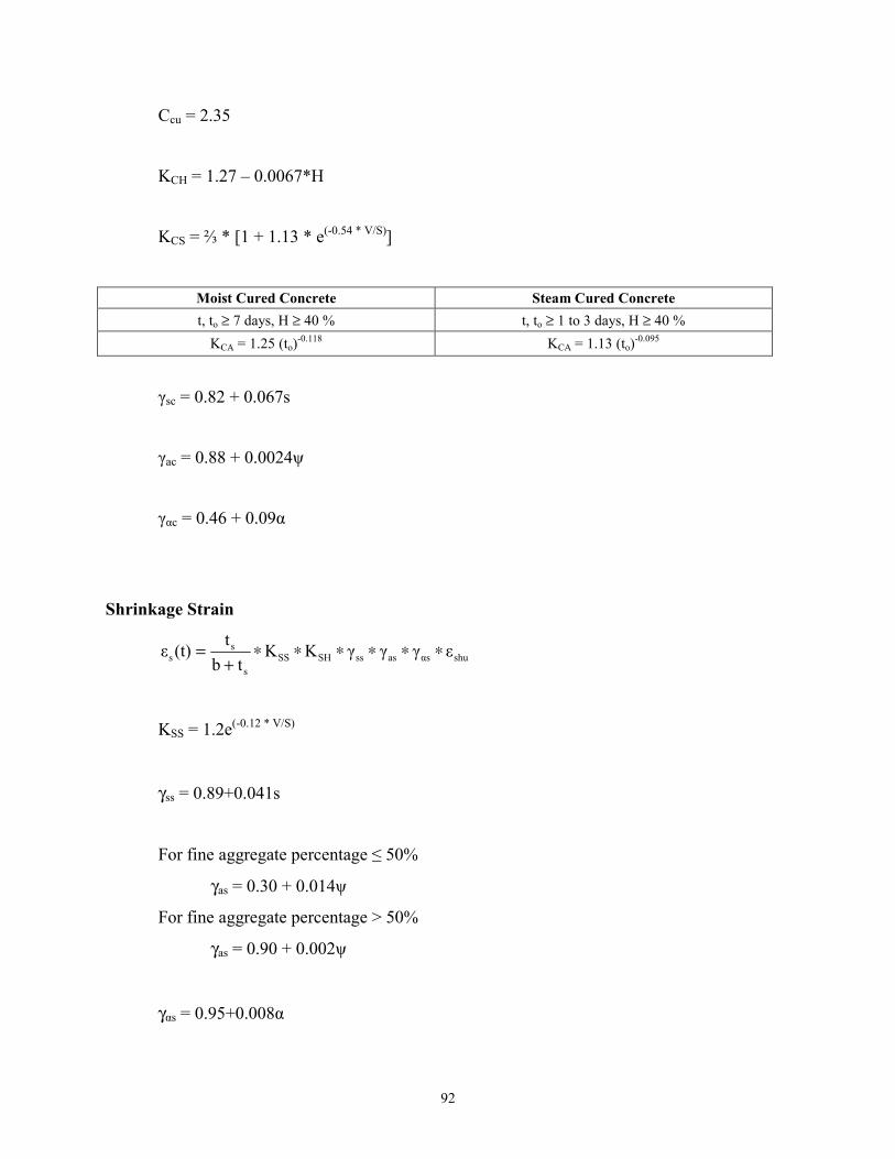
92

Ccu = 2.35

KCH = 1.27 – 0.0067*H

KCS = ⅔ * [1 + 1.13 * e(-0.54 * V/S)]

Moist Cured Concrete Steam Cured Concrete t, to ≥ 7 days, H ≥ 40 % t, to ≥ 1 to 3 days, H ≥ 40 %

KCA = 1.25 (to)-0.118 KCA = 1.13 (to)-0.095

γsc = 0.82 + 0.067s

γac = 0.88 + 0.0024ψ

γαc = 0.46 + 0.09α

Shrinkage Strain

shuαsasssSHSSs

ss εγγγKK

tbt(t)ε ∗∗∗∗∗∗+

=

KSS = 1.2e(-0.12 * V/S)

↑

γss = 0.89+0.041s↑

For fine aggregate percentage ≤ 50%

γas = 0.30 + 0.014ψ

For fine aggregate percentage > 50%↑

γas = 0.90 + 0.002ψ↑

↑

γαs = 0.95+0.008α

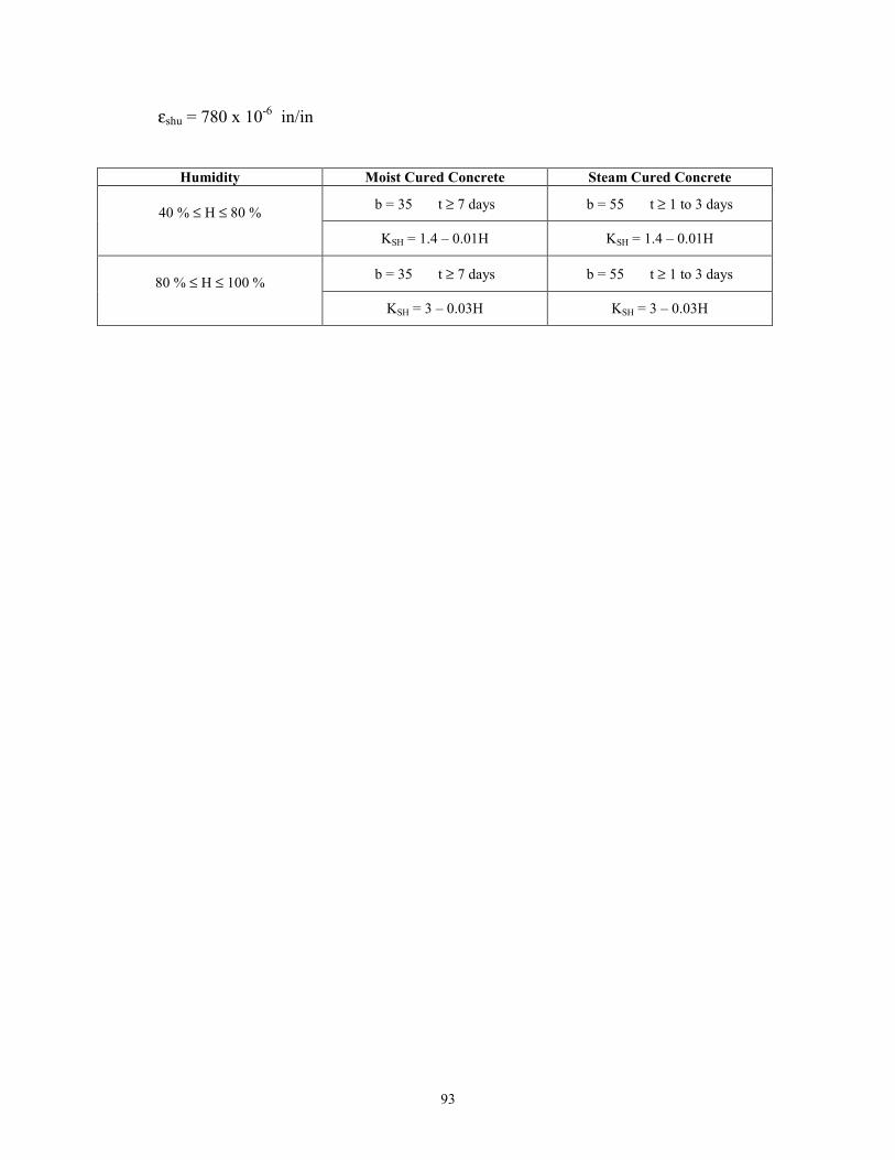
93

εshu = 780 x 10-6 in/in

Humidity Moist Cured Concrete Steam Cured Concrete

40 % ≤ H ≤ 80 % b = 35 t ≥ 7 days b = 55 t ≥ 1 to 3 days

KSH = 1.4 – 0.01H KSH = 1.4 – 0.01H

80 % ≤ H ≤ 100 % b = 35 t ≥ 7 days b = 55 t ≥ 1 to 3 days

KSH = 3 – 0.03H KSH = 3 – 0.03H

94

CEB 90 Code Model

Nomenclature

φ(t,to) = Creep coefficient defining creep between time t and to

Ec = Modulus of elasticity at 28 days (N/mm2)

Ec(to) = Modulus of elasticity at age of loading (N/mm2)

ε(t) = Total strain; instantaneous plus creep and shrinkage (mm/mm)

εcs(t-ts) = Shrinkage strain between time t and ts (mm/mm)

t = Age of concrete after casting (days)

ts = Age of concrete at the beginning of shrinkage (days)

fcm = Mean 28 day concrete compressive strength (N/mm2)

fck = Characteristic compressive strength with 95% confidence (N/mm2)

to = Age of concrete at loading (days)

φo = Notional creep coefficient

βc(t-to) = Coefficient describing creep development with time after loading

φRH = Factor to allow for relative humidity on the notional creep coefficient (φo)

β(fcm) = Factor to allow for effect of concrete strength on the notional creep coefficient

(φo)

β(to) = Factor to allow for the effect of age of concrete at loading on the notional creep

coefficient (φo)

RH = Relative humidity (%)

Ac = Cross-section area of member (mm2)

u = Perimeter of member in contact with the atmosphere (mm)

ho = 2Ac/u = Notional size of member (mm)

βH = Coefficient to allow for the effect of relative humidity and the notional member

size (ho) on creep

εcso = Notional shrinkage coefficient

βs(t-ts) = Equation describing development of shrinkage with time

εs(fcm) = Factor to allow for the effect of concrete strength on shrinkage

95

βRH = Coefficient to allow for the effect of relative humidity on the notional shrinkage

coefficient (εcso)

βsc = Coefficient depending on type of cement

βs = Coefficient to describe the development of shrinkage with time

σ = Applied stress (N/mm2)

α = Coefficient for cement type

to,T = temperature adjusted age of concrete at loading (days)

∆ti = number of days at temperature T

T(∆ti) = temperature during time period ∆ti (oC)

n = number of time intervals considered

96

CEB 90 Model Code Equations

Total Strain

ε(t) = εcs (t-ts) +

+

φ)(tE

1E

)t(t,

occ

o σ

Mean Concrete Strength

fcm = fck + 8 N/mm2

Note: Estimate not needed. The experimental f’c28 was used.

Modulus of Elasticity at Age t

Ec =10000 3cmf

Ec(to) = (Ec)

)

t28-(1

2S

e

0.38, slow hardening cement S = 0.25, normal and rapid hardening cement 0.20, rapid hardening high strength

Note: Estimate not needed. The experimental Ec and Ec(to) was used.


Compliance function [µε/ psi] = )(tE

1E

)t(t,

occ

o +φ

φ (t,to) = (φo) * βc(t-to)

φo = φRH * β(fcm) * β(to)

φRH = 3

oh0.1

)100

(11

∗

−+

RH

97

β(fcm) = cmf8.16

β(to) = )1.0(

12.0

0t+

βc(t-to) = [ ]0.3oΗ

0.3o

)t(tβ)t(t

−+−

βH = 1.5 * [1 + (0.012 * RH)18] (ho) + 250 ≤ 1500 days

The effect of cement type can be modified for the creep coefficient by modifying the age

at loading:

to = to,T * α

+

+1

)(t29

1.2To,

≥ 0.5 days

to,T =

−

+−

=∑

13.65)T(∆273

4000n

1ii

ie *∆t

Cement Type α

SL -1 N, R 0 RS 1

98

Shrinkage Strain

εcs(t – ts) = (εcso) * βs (t – ts)

εcso = εs (fcm) * (βRH)

εs (fcm) = [160 + βsc (90 – fcm)] * 10-6

Type of Cement ββββsc

Slow hardening (SL) 4 Normal and rapid hardening (N, R) 5 Rapid hardening high strength (RS) 8

Humidity ββββRH

40 % ≤ RH ≤ 99 %, stored in air -1.55 x βsRH

RH ≥ 99 %, immersed in water 0.25

βRH = 1 – 3

100RH

βs(t-ts) = [ ])t(th0.035)t(t

s20

s

−+∗−

99

The B3 Model

Nomenclature J(t,t’) = Creep compliance function; creep plus elastic (always x10-6/psi)

α = Thermal expansion coefficient

∆T(t) = Temperature change from reference at time t

Co(t,t’) = Compliance function for basic creep

Cd(t,t’,to) = Compliance function for additional creep due to drying

ε(t) = Total Strain; instantaneous plus creep and drying (in/in)

εsh(t) = Shrinkage Strain (in./in.)

f’c = Mean 28 day concrete compressive strength (psi)

fck = Specified concrete compressive strength at 28 days (psi)

E28 = Modulus of elasticity at 28 days (psi)

q1 = Instantaneous strain due to unit stress

q2 = Aging visco-elastic compliance

q3 = Non-aging visco-elastic compliance

q4 = Flow compliance

q5 = Creep at drying


t’ = Age of concrete at loading (days)

to = Age of concrete at the beginning of shrinkage (days)

c = Cement content of concrete (lbs/ft3)

w/c = Water to cement ratio by weight

a/c = Aggregate to cement ratio by weight

H(t) = Spatial average of pore relative humidity within cross section

S(t) = Time function for shrinkage

εsh∞ = Ultimate shrinkage strain (negative, always x 10-6 in./in.)

w = Water content of concrete (lbs/ft3)

h = Relative humidity (decimal)

τsh = Shrinkage half-time (days)

ks = Cross section shape factor

100

V/S = Volume to surface are ratio (in.)

D = 2(V/S) = Effective cross-section thickness (in.)

kh = Humidity function for shrinkage

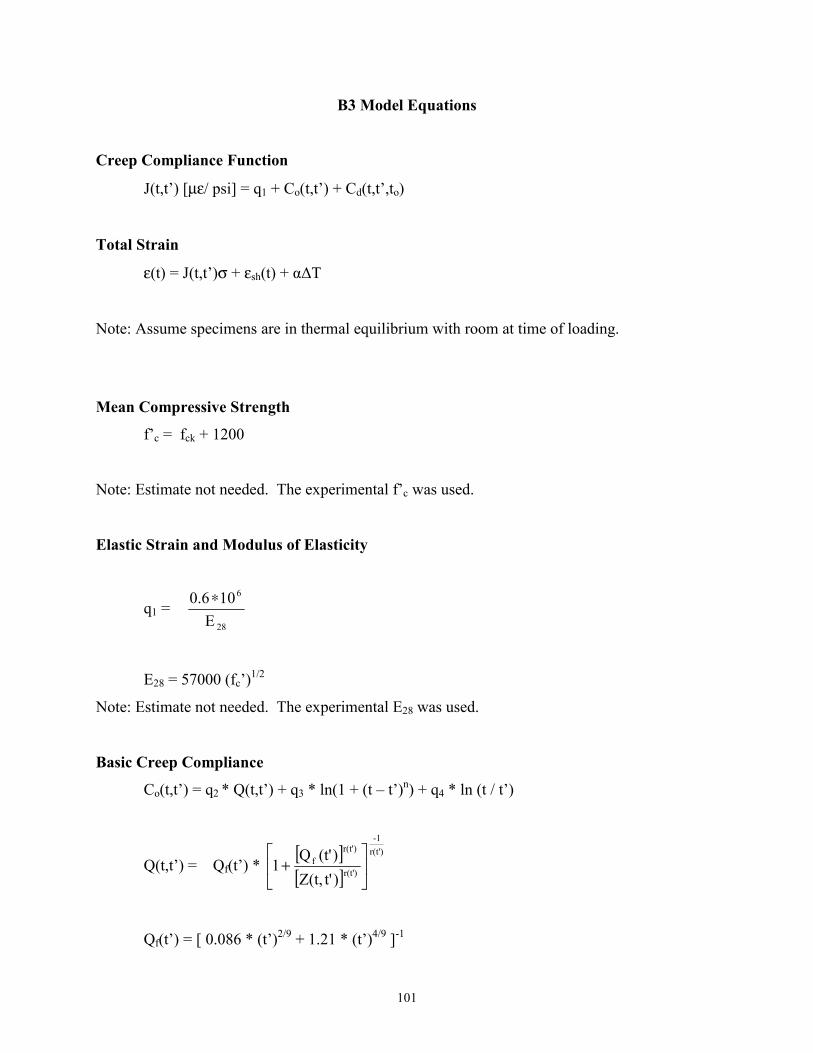
101

B3 Model Equations


J(t,t’) [µε/ psi] = q1 + Co(t,t’) + Cd(t,t’,to)

Total Strain

ε(t) = J(t,t’)σ + εsh(t) + α∆T

Note: Assume specimens are in thermal equilibrium with room at time of loading.

Mean Compressive Strength

f’c = fck + 1200

Note: Estimate not needed. The experimental f’c was used.

Elastic Strain and Modulus of Elasticity

q1 = 28

6

E106.0 ∗

E28 = 57000 (fc’)1/2

Note: Estimate not needed. The experimental E28 was used.

Basic Creep Compliance

Co(t,t’) = q2 * Q(t,t’) + q3 * ln(1 + (t – t’)n) + q4 * ln (t / t’)

Q(t,t’) = Qf(t’) * [ ][ ]

)r(t'-1

)r(t'

)r(t'f

)t'Z(t,)(t'Q1

+

Qf(t’) = [ 0.086 * (t’)2/9 + 1.21 * (t’)4/9 ]-1

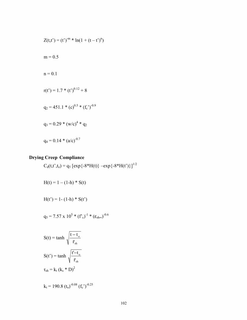
102

Z(t,t’) = (t’)-m * ln(1 + (t – t’)n)

m = 0.5

n = 0.1

r(t’) = 1.7 * (t’)0.12 + 8

q2 = 451.1 * (c)0.5 * (fc’)-0.9

q3 = 0.29 * (w/c)4 * q2

q4 = 0.14 * (a/c)-0.7

Drying Creep Compliance

Cd(t,t’,to) = q5 [exp{-8*H(t)} –exp{-8*H(t’)}]1/2

H(t) = 1 – (1-h) * S(t)

H(t’) = 1- (1-h) * S(t’)

q5 = 7.57 x 105 * (f’c)-1 * (εsh∞)-0.6

S(t) = tanh sh

ottτ−

S(t’) = tanh sh

ott'τ−

τsh = kt (ks * D)2

kt = 190.8 (to)-0.08 (fc’)-0.25

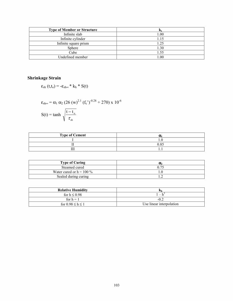
103

Type of Member or Structure ks Infinite slab 1.00

Infinite cylinder 1.15 Infinite square prism 1.25

Sphere 1.30 Cube 1.55

Undefined member 1.00

Shrinkage Strain

εsh (t,to) = -εsh∞ * kh * S(t)

εsh∞ = α1 α2 (26 (w)2.1 (fc’)-0.28 + 270) x 10-6

S(t) = tanh sh

ottτ−

Type of Cement αααα1

I 1.0 II 0.85 III 1.1

Type of Curing αααα2 Steamed cured 0.75

Water cured or h = 100 % 1.0 Sealed during curing 1.2

Relative Humidity kh

for h ≤ 0.98 1 – h3

for h = 1 -0.2 for 0.98 ≤ h ≤ 1 Use linear interpolation

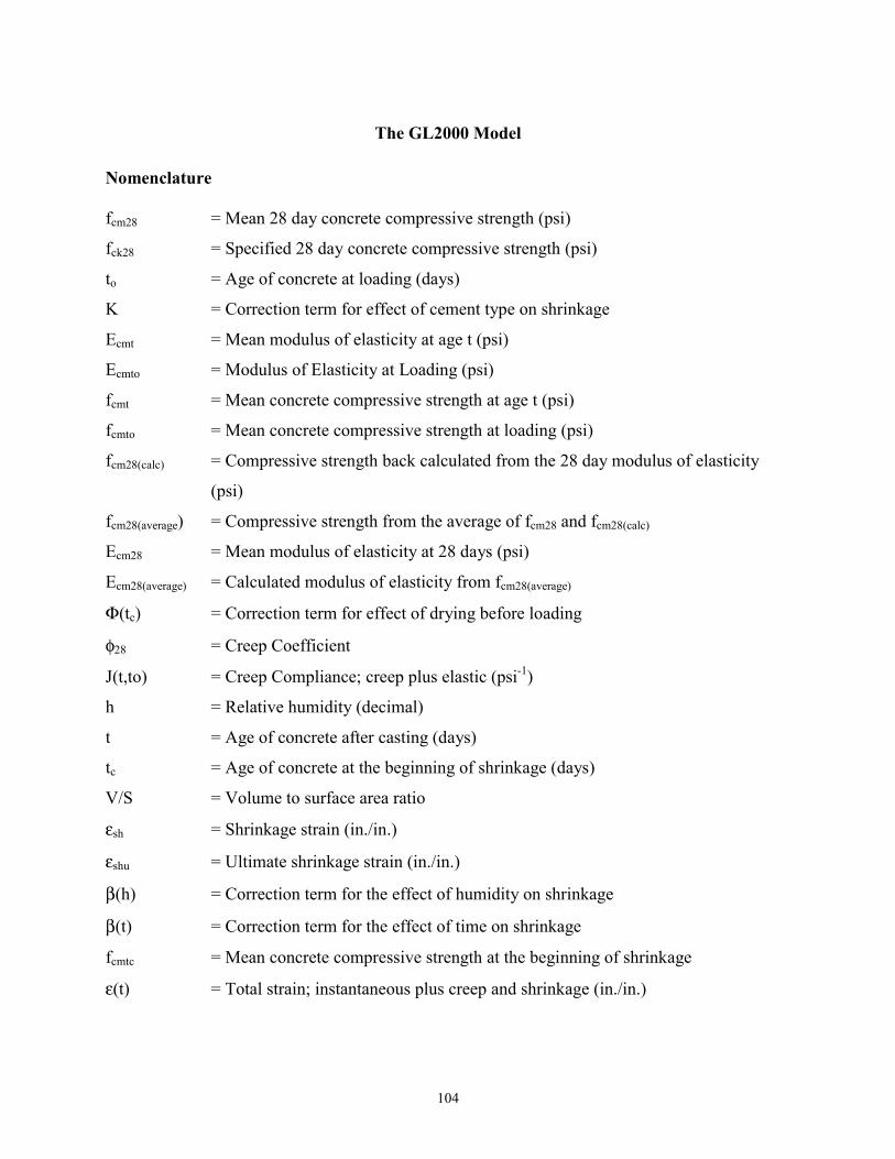
104

The GL2000 Model

Nomenclature fcm28 = Mean 28 day concrete compressive strength (psi)

fck28 = Specified 28 day concrete compressive strength (psi)

to = Age of concrete at loading (days)

K = Correction term for effect of cement type on shrinkage

Ecmt = Mean modulus of elasticity at age t (psi)

Ecmto = Modulus of Elasticity at Loading (psi)

fcmt = Mean concrete compressive strength at age t (psi)

fcmto = Mean concrete compressive strength at loading (psi)

fcm28(calc) = Compressive strength back calculated from the 28 day modulus of elasticity

(psi)

fcm28(average) = Compressive strength from the average of fcm28 and fcm28(calc)

Ecm28 = Mean modulus of elasticity at 28 days (psi)

Ecm28(average) = Calculated modulus of elasticity from fcm28(average)

Φ(tc) = Correction term for effect of drying before loading

φ28 = Creep Coefficient

J(t,to) = Creep Compliance; creep plus elastic (psi-1)

h = Relative humidity (decimal)


tc = Age of concrete at the beginning of shrinkage (days)

V/S = Volume to surface area ratio

εsh = Shrinkage strain (in./in.)

εshu = Ultimate shrinkage strain (in./in.)

β(h) = Correction term for the effect of humidity on shrinkage

β(t) = Correction term for the effect of time on shrinkage

fcmtc = Mean concrete compressive strength at the beginning of shrinkage

ε(t) = Total strain; instantaneous plus creep and shrinkage (in./in.)

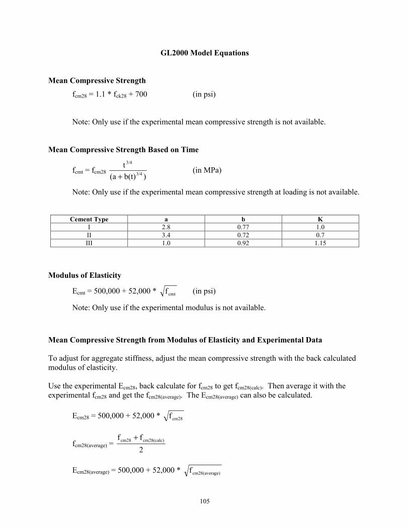
105

GL2000 Model Equations

Mean Compressive Strength

fcm28 = 1.1 * fck28 + 700 (in psi)

Note: Only use if the experimental mean compressive strength is not available.

Mean Compressive Strength Based on Time

fcmt = fcm28 )b(t)(a

t3/4

3/4

+ (in MPa)

Note: Only use if the experimental mean compressive strength at loading is not available.

Cement Type a b K

I 2.8 0.77 1.0 II 3.4 0.72 0.7 III 1.0 0.92 1.15

Modulus of Elasticity

Ecmt = 500,000 + 52,000 * cmtf (in psi)

Note: Only use if the experimental modulus is not available.

Mean Compressive Strength from Modulus of Elasticity and Experimental Data To adjust for aggregate stiffness, adjust the mean compressive strength with the back calculated modulus of elasticity. Use the experimental Ecm28, back calculate for fcm28 to get fcm28(calc). Then average it with the experimental fcm28 and get the fcm28(average). The Ecm28(average) can also be calculated. Ecm28 = 500,000 + 52,000 * cm28f

fcm28(average) = 2ff cm28(calc)cm28 +

Ecm28(average) = 500,000 + 52,000 * ge)cm28(averaf

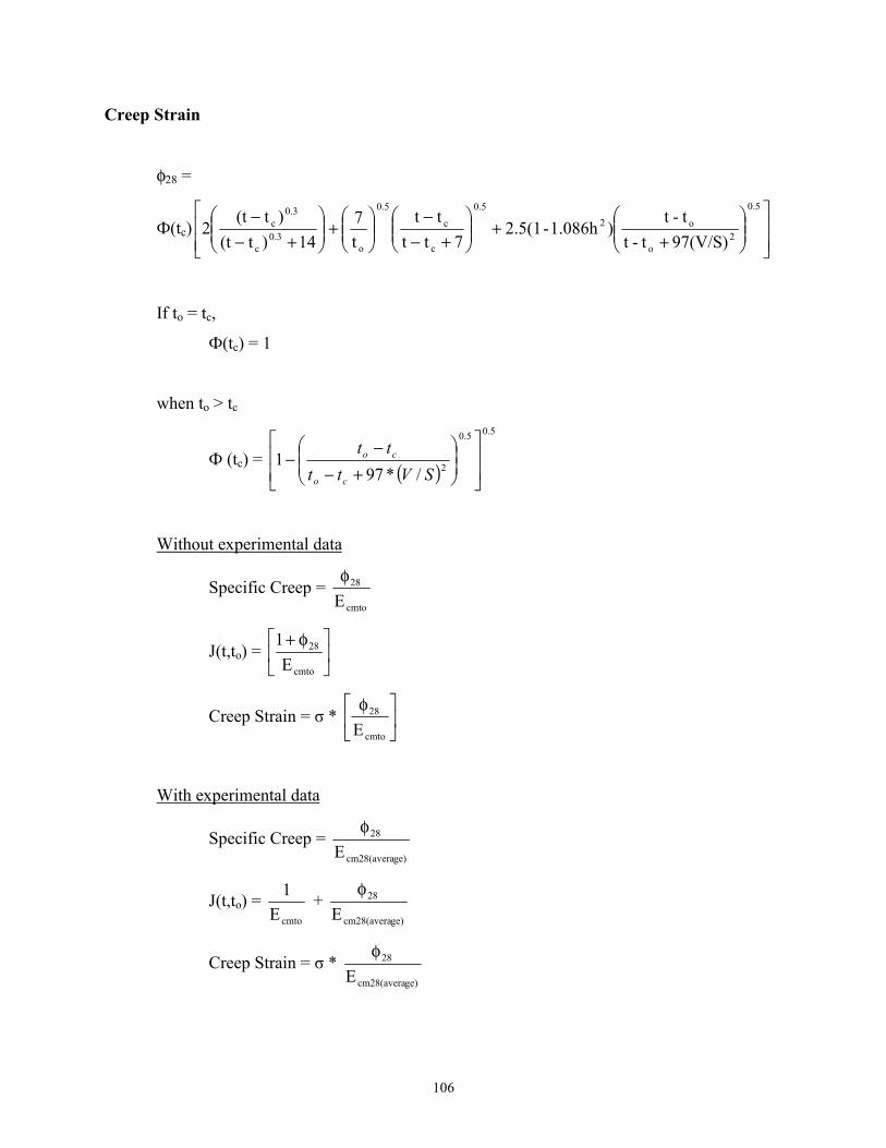
106

Creep Strain

φ28 =

Ф(tc)

++

+−−

+

+−−

0.5

2o

o20.5

c

c

0.5

o0.3

c

0.3c

97(V/S)t-tt-t

)1.086h-2.5(17tt

ttt7

14)t(t)t(t

2

If to = tc,

Ф(tc) = 1

when to > tc

Ф (tc) = ( )

5.05.0

2/*971

+−−

−SVtt

tt

co

co

Without experimental data

Specific Creep = cmto

28

Εφ

J(t,to) =

φ+

cmto

28

E1

Creep Strain = σ * ��

��

� φ

cmto

28

E

With experimental data

Specific Creep = ge)cm28(avera

28

Εφ

J(t,to) = cmtoE1 +

ge)cm28(avera

28

Εφ

Creep Strain = σ * ge)cm28(avera

28

Εφ

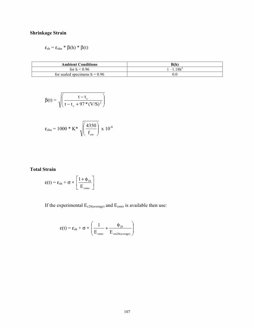
107

Shrinkage Strain

εsh = εshu * β(h) * β(t)

Ambient Conditions Β(h)

for h < 0.96 1 –1.18h4 for sealed specimens h = 0.96 0.0

β(t) =

+−−

2c

c

(V/S) * 97tttt

εshu = 1000 * K*

cmf4350 x 10-6

Total Strain

ε(t) = εsh + σ ∗

φ+

cmto

28

E1

If the experimental Ec28(average) and Ecmto is available then use:

ε(t) = εsh + σ ∗

φ+

ge)cm28(avera

28

cmto EE1

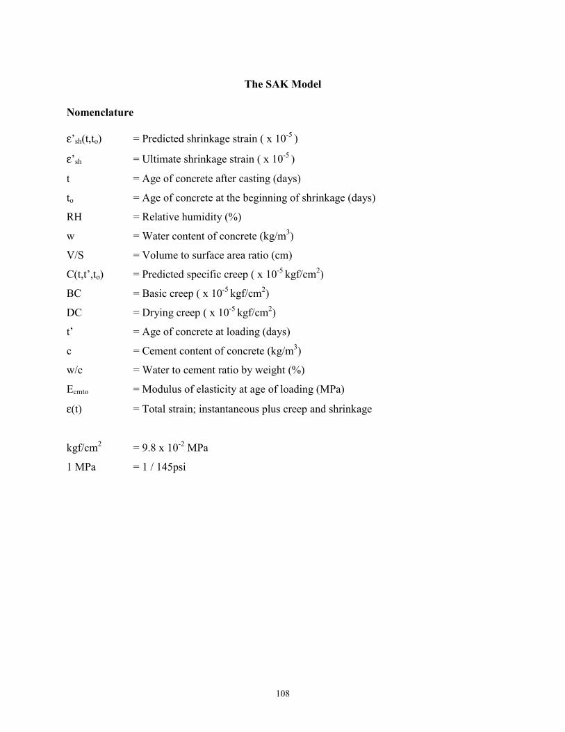
108

The SAK Model

Nomenclature ε’sh(t,to) = Predicted shrinkage strain ( x 10-5 )

ε’sh = Ultimate shrinkage strain ( x 10-5 )


to = Age of concrete at the beginning of shrinkage (days)

RH = Relative humidity (%)

w = Water content of concrete (kg/m3)

V/S = Volume to surface area ratio (cm)

C(t,t’,to) = Predicted specific creep ( x 10-5 kgf/cm2)

BC = Basic creep ( x 10-5 kgf/cm2)

DC = Drying creep ( x 10-5 kgf/cm2)

t’ = Age of concrete at loading (days)

c = Cement content of concrete (kg/m3)

w/c = Water to cement ratio by weight (%)

Ecmto = Modulus of elasticity at age of loading (MPa)

ε(t) = Total strain; instantaneous plus creep and shrinkage

kgf/cm2 = 9.8 x 10-2 MPa

1 MPa = 1 / 145psi

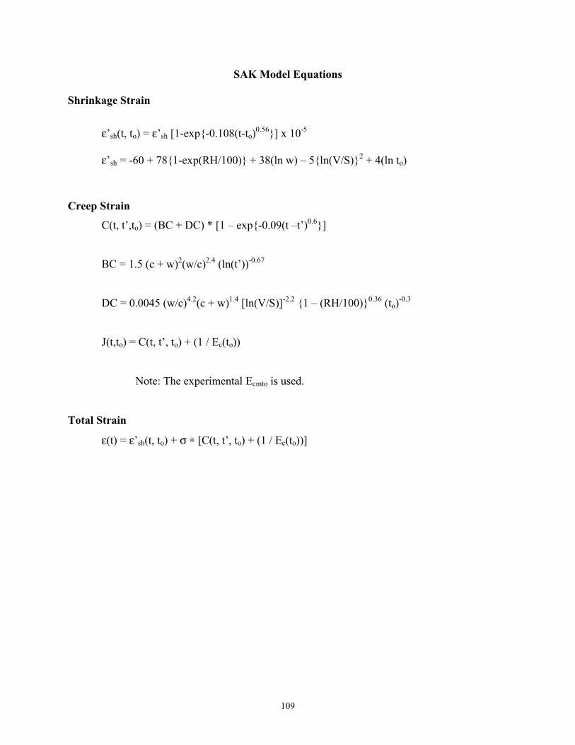
109

SAK Model Equations

Shrinkage Strain

ε’sh(t, to) = ε’sh [1-exp{-0.108(t-to)0.56}] x 10-5

ε’sh = -60 + 78{1-exp(RH/100)} + 38(ln w) – 5{ln(V/S)}2 + 4(ln to)

Creep Strain

C(t, t’,to) = (BC + DC) * [1 – exp{-0.09(t –t’)0.6}]

BC = 1.5 (c + w)2(w/c)2.4 (ln(t’))-0.67

DC = 0.0045 (w/c)4.2(c + w)1.4 [ln(V/S)]-2.2 {1 – (RH/100)}0.36 (to)-0.3

J(t,to) = C(t, t’, to) + (1 / Ec(to))

Note: The experimental Ecmto is used.

Total Strain

ε(t) = ε’sh(t, to) + σ ∗ [C(t, t’, to) + (1 / Ec(to))]

110

REFERENCES ACI 209R-92, Prediction of Creep, Shrinkage, and Temperature Effects in Concrete Structures,

ACI Manual of Concrete Practice Part 1, 2002.

ACI 213R-87, Guide to Structural Lightweight Aggregate Concrete, ACI Manual of Concrete

Practice, Part 1, 2002.

Bazant, Z. P. and Baweja, S., Creep and shrinkage prediction model for analysis and design of

concrete structures – model B3, RILEM Recommendation, Materials and Structures, v.

28, 1995, pp. 357-365.

Bazant, Z. P. and Baweja, S., Justification and refinements of Model B3 for concrete creep and

shrinkage 1. Statistics and Sensitivity, Materials and Structures, v. 28, 1995, pp. 415-430.

Bazant, Z. P. and Baweja, S., Justification and refinements of Model B3 for concrete creep and

shrinkage 2. Updating and theoretical basis, Materials and Structures, v. 28, 1995, pp.

488-495.

CEB-FIP Model Code, Evaluation of the Time Dependent Behavior of Concrete, September

1990.

Gardner, N. J. and Lockman, M. J., Design Provisions for Drying Shrinkage and Creep of

Normal-Strength Concrete, ACI Materials Journal, v. 98, March-April 2001, pp. 159-167.

Gilbert, R.I., Time Effects in Concrete Structures, Developments in Civil Engineering, v. 23,

1988.

Huo, X. S., Al-Omaishi, N., and Tadros, M.K., Creep , Shrinkage, Modulus of Elasticity of High

Performance Concrete., ACI Materials Journal, v. 98, n.6, November-December 2001.

111

Lakshmikantan, S., Evaluation of Concrete Shrinkage and Creep Models, Masters of Science

Thesis in Civil Engineering, San Jose State University, May 1999.

Mehta, P. K., and Monteiro, P. J. M., Concrete Structure, Properties, and Materials, Second

Edition, Prentice Hall, 1993.

Meyerson, R., Compressive Creep of Prestressed Concrete Mixtures with and without Mineral

Admixtures, Master of Science Thesis in Civil Engineering, Virginia Tech, February

2001.

Mokarem, D. W., Development of Concrete Shrinkage Performance Specifications, Doctor of

Philosophy in Civil Engineering, Virginia Tech, May 2002.

Myers, J. J., and Yang, Y., Practical Issues for the Application of High-Performance Concrete to

Highway Structures," Journal of Bridge Engineering, v. 6, n. 6, 2001.

Nawy, E. G., Fundamentals of High-Performance Concrete, John Wiley & Sons, Inc., New York,

2nd ed., 2001

Lakshmikantan, S., Evaluation of Concrete Shrinkage and Creep Models, Master of Science in

Civil Engineering, San Jose State University, May 1999.

Neville, A. M., Dilger, W. H., and Brooks, J. J., Creep of Plain and Structural Concrete,

Construction Press, New York, 1983.

Sakata, K., Prediction of Creep and Shrinkage, Creep and Shrinkage of Concrete, Proceedings of

the Fifth International RILEM Symposium, Barcelona Spain, pp. 649-654, September 6-

9, 1993.

Structural Lightweight Aggregate Concrete, edited by Clarke, J. L., Blackie Academic

Professional, London, 1993.

112

APPENDIX B

Mixing and Curing Data

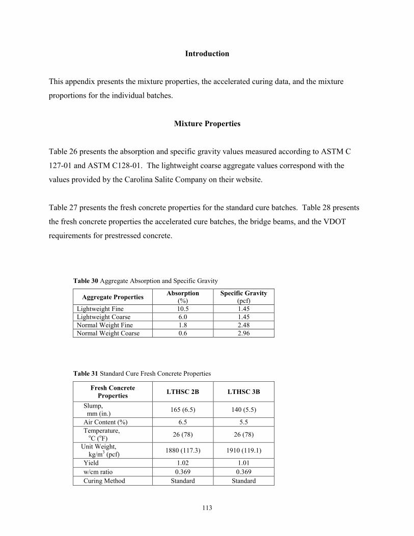
113

Introduction

This appendix presents the mixture properties, the accelerated curing data, and the mixture

proportions for the individual batches.

Mixture Properties

Table 26 presents the absorption and specific gravity values measured according to ASTM C

127-01 and ASTM C128-01. The lightweight coarse aggregate values correspond with the

values provided by the Carolina Salite Company on their website.

Table 27 presents the fresh concrete properties for the standard cure batches. Table 28 presents

the fresh concrete properties the accelerated cure batches, the bridge beams, and the VDOT

requirements for prestressed concrete.

Table 30 Aggregate Absorption and Specific Gravity

Aggregate Properties Absorption (%)

Specific Gravity (pcf)

Lightweight Fine 10.5 1.45 Lightweight Coarse 6.0 1.45 Normal Weight Fine 1.8 2.48 Normal Weight Coarse 0.6 2.96

Table 31 Standard Cure Fresh Concrete Properties

Fresh Concrete Properties LTHSC 2B LTHSC 3B

Slump, mm (in.) 165 (6.5) 140 (5.5)

Air Content (%) 6.5 5.5 Temperature, oC (oF) 26 (78) 26 (78)

Unit Weight, kg/m3 (pcf) 1880 (117.3) 1910 (119.1)

Yield 1.02 1.01 w/cm ratio 0.369 0.369 Curing Method Standard Standard

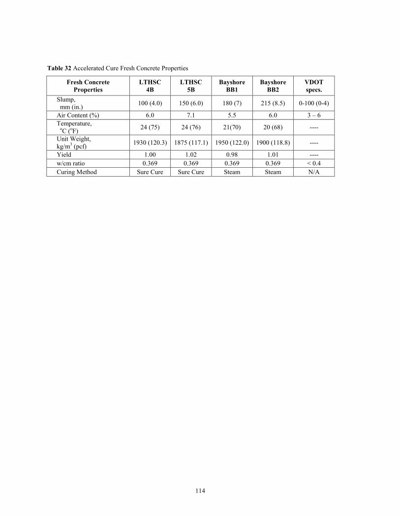
114

Table 32 Accelerated Cure Fresh Concrete Properties

Fresh Concrete Properties

LTHSC 4B

LTHSC 5B

Bayshore BB1

Bayshore BB2

VDOT specs.

Slump, mm (in.) 100 (4.0) 150 (6.0) 180 (7) 215 (8.5) 0-100 (0-4)

Air Content (%) 6.0 7.1 5.5 6.0 3 – 6 Temperature, oC (oF) 24 (75) 24 (76) 21(70) 20 (68) ----

Unit Weight, kg/m3 (pcf) 1930 (120.3) 1875 (117.1) 1950 (122.0) 1900 (118.8) ----

Yield 1.00 1.02 0.98 1.01 ---- w/cm ratio 0.369 0.369 0.369 0.369 < 0.4 Curing Method Sure Cure Sure Cure Steam Steam N/A

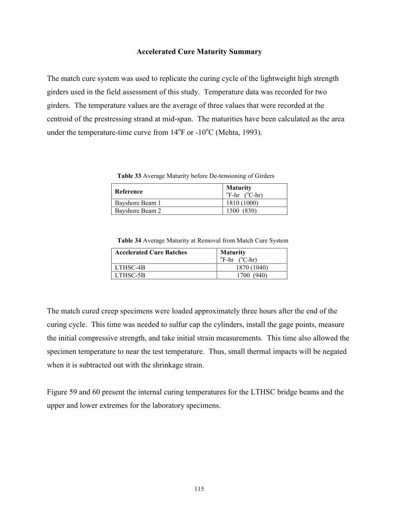
115

Accelerated Cure Maturity Summary

The match cure system was used to replicate the curing cycle of the lightweight high strength

girders used in the field assessment of this study. Temperature data was recorded for two

girders. The temperature values are the average of three values that were recorded at the

centroid of the prestressing strand at mid-span. The maturities have been calculated as the area

under the temperature-time curve from 14oF or -10oC (Mehta, 1993).

Table 33 Average Maturity before De-tensioning of Girders

Reference Maturity oF-hr (oC-hr)

Bayshore Beam 1 1810 (1000) Bayshore Beam 2 1500 (830)

Table 34 Average Maturity at Removal from Match Cure System

Accelerated Cure Batches Maturity oF-hr (oC-hr)

LTHSC-4B 1870 (1040) LTHSC-5B 1700 (940)

The match cured creep specimens were loaded approximately three hours after the end of the

curing cycle. This time was needed to sulfur cap the cylinders, install the gage points, measure

the initial compressive strength, and take initial strain measurements. This time also allowed the

specimen temperature to near the test temperature. Thus, small thermal impacts will be negated

when it is subtracted out with the shrinkage strain.

Figure 59 and 60 present the internal curing temperatures for the LTHSC bridge beams and the

upper and lower extremes for the laboratory specimens.

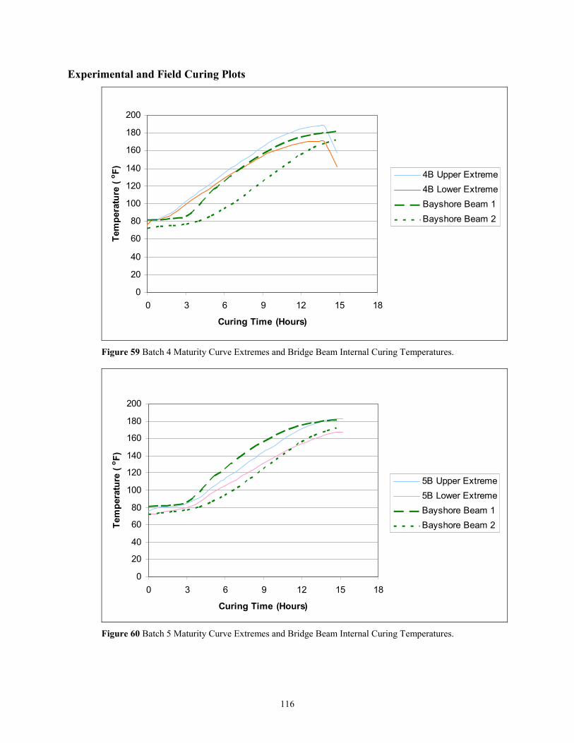
116

Experimental and Field Curing Plots

0

20

40

60

80

100

120

140

160

180

200

0 3 6 9 12 15 18

Curing Time (Hours)

Tem

pera

ture

(o F) 4B Upper Extreme

4B Lower ExtremeBayshore Beam 1Bayshore Beam 2

Figure 59 Batch 4 Maturity Curve Extremes and Bridge Beam Internal Curing Temperatures.

0

20

40

60

80

100

120

140

160

180

200

0 3 6 9 12 15 18

Curing Time (Hours)

Tem

pera

ture

(o F)

5B Upper Extreme5B Lower ExtremeBayshore Beam 1Bayshore Beam 2

Figure 60 Batch 5 Maturity Curve Extremes and Bridge Beam Internal Curing Temperatures.

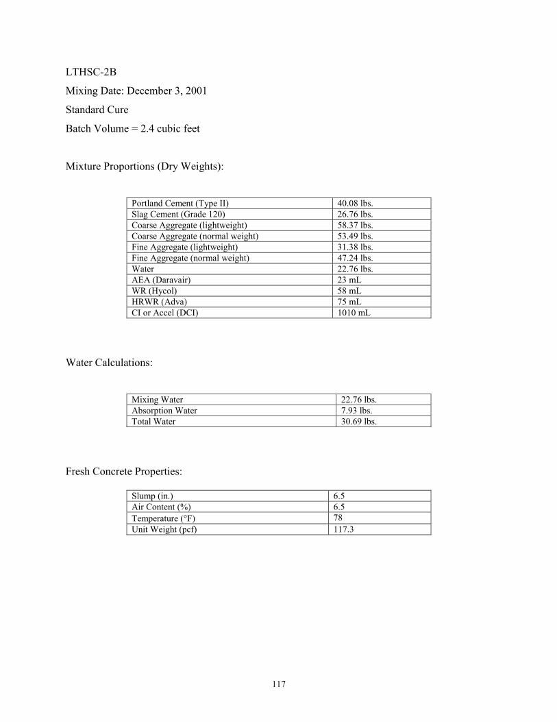
117

LTHSC-2B

Mixing Date: December 3, 2001

Standard Cure

Batch Volume = 2.4 cubic feet

Mixture Proportions (Dry Weights):

Portland Cement (Type II) 40.08 lbs. Slag Cement (Grade 120) 26.76 lbs. Coarse Aggregate (lightweight) 58.37 lbs. Coarse Aggregate (normal weight) 53.49 lbs. Fine Aggregate (lightweight) 31.38 lbs. Fine Aggregate (normal weight) 47.24 lbs. Water 22.76 lbs. AEA (Daravair) 23 mL WR (Hycol) 58 mL HRWR (Adva) 75 mL CI or Accel (DCI) 1010 mL

Water Calculations:

Mixing Water 22.76 lbs. Absorption Water 7.93 lbs. Total Water 30.69 lbs.

Fresh Concrete Properties:

Slump (in.) 6.5 Air Content (%) 6.5 Temperature (°F) 78 Unit Weight (pcf) 117.3

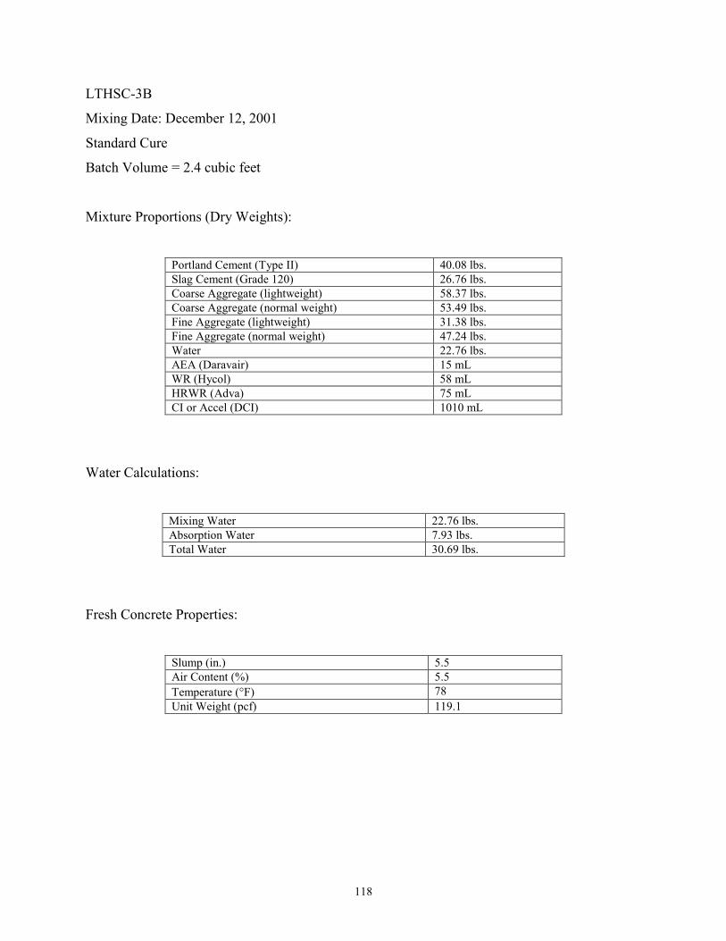
118

LTHSC-3B

Mixing Date: December 12, 2001

Standard Cure




Water Calculations:




119

LTHSC-4B

Mixing Date: February 17, 2002

Accelerated Cure




Water Calculations:




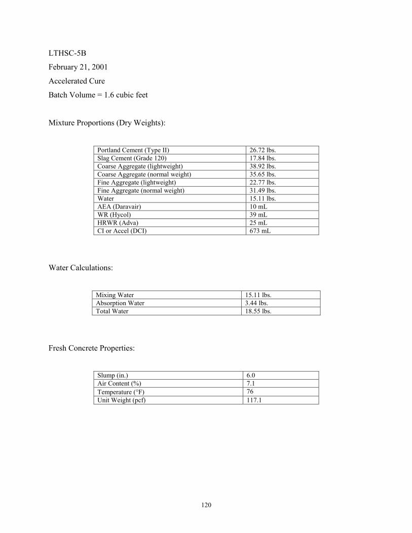
120

LTHSC-5B

February 21, 2001

Accelerated Cure




Water Calculations:




121

APPENDIX C

Photographs

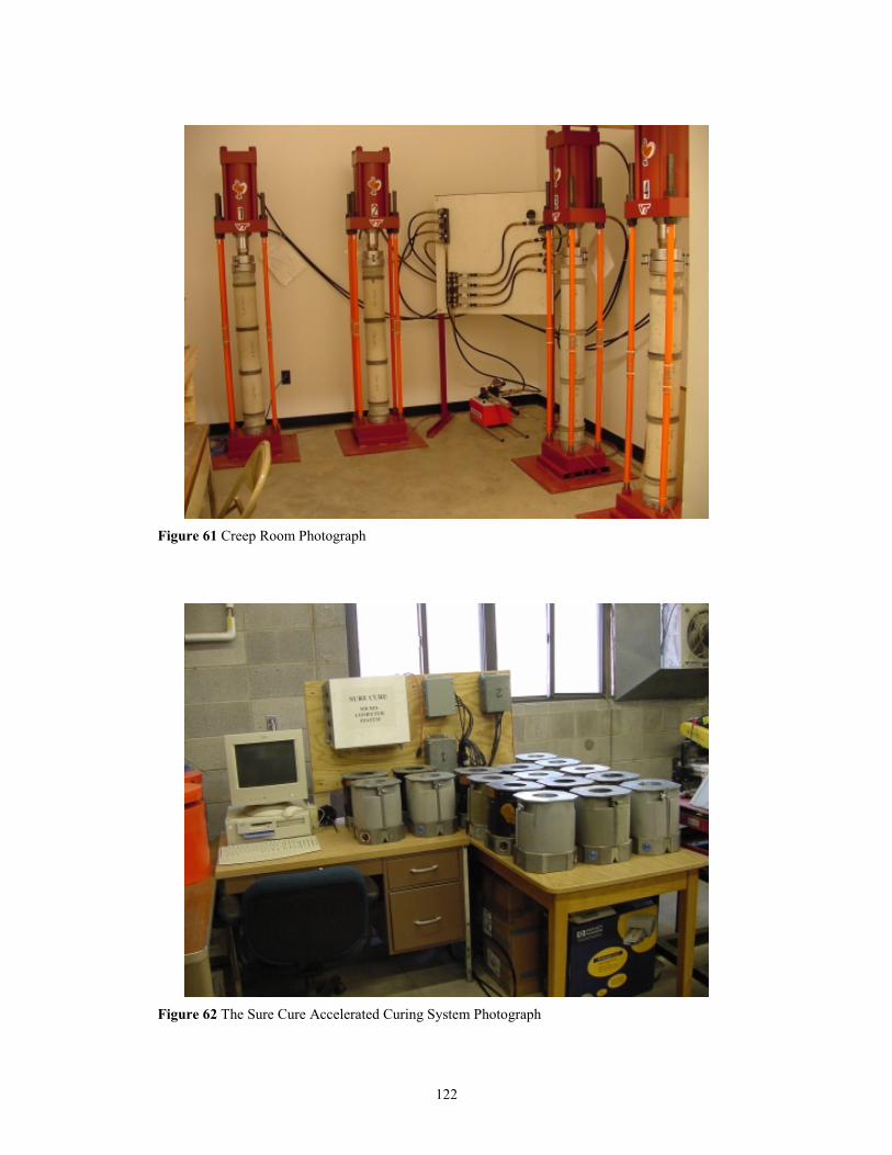
122

Figure 61 Creep Room Photograph

Figure 62 The Sure Cure Accelerated Curing System Photograph

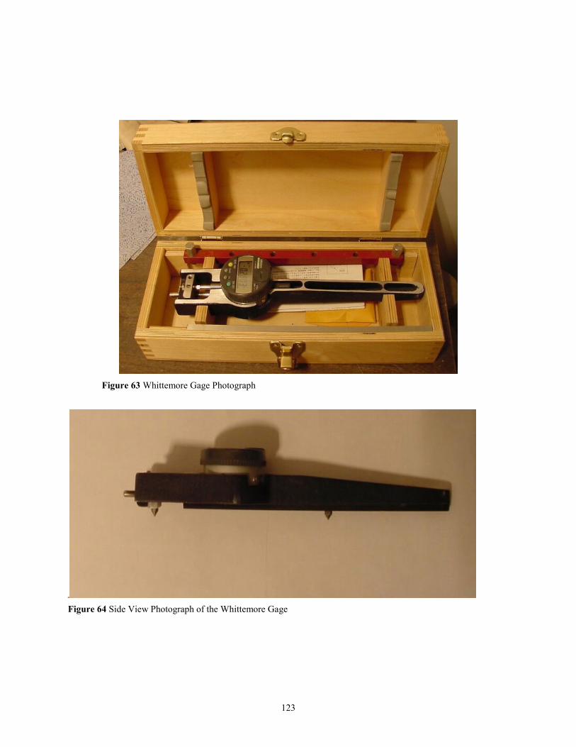
123

Figure 63 Whittemore Gage Photograph

Figure 64 Side View Photograph of the Whittemore Gage

124

APPENDIX D

Creep Frame Calibration

125

Creep Frame Calibration

The four creep frames were built and calibrated by Richard Meyerson and David Mokarem. The

hydraulic pressure gage for frame 3 was replaced so recalibration of frame three was required.

Details of Meyerson’s calibration can be found in his thesis, Compressive Creep of Prestressed

Concrete Mixtures with and without Mineral Admixtures.

Figures 63, 64, and 66 are from Meyerson’s thesis and represent the current calibration of frames

1, 2, and 4, respectively.

The calibration of frame three was conducted by measuring strains, applied loads and the

hydraulic gage pressure. The frames have four vertical rods with 350 ohm strain gages attached.

The gage factor is 2.090 ± 0.5% at 24oC. The applied load was measure with a 60 kip load cell.

The frame was loaded in 5 kip increments up to 55 kips. This repeated with two different load

cells.

Figure 65 presents the applied load vs. the gage pressure for frame 3. The calibration chart is the

average measurement of two load cells. The strain in the rods was also measured and the

calculated load verse applied load was checked.

A photograph of the frames is in Appendix C.

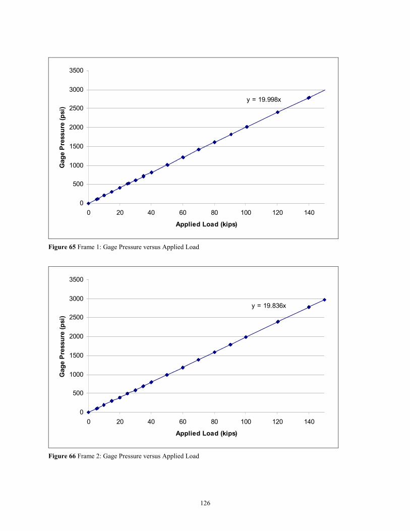
126

y = 19.998x

0

500

1000

1500

2000

2500

3000

3500

0 20 40 60 80 100 120 140

Applied Load (kips)

Gag

e Pr

essu

re (p

si)

Figure 65 Frame 1: Gage Pressure versus Applied Load

y = 19.836x

0

500

1000

1500

2000

2500

3000

3500

0 20 40 60 80 100 120 140

Applied Load (kips)

Gag

e Pr

essu

re (p

si)


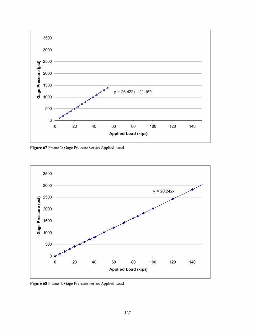
127

y = 26.422x - 21.159

0

500

1000

1500

2000

2500

3000

3500

0 20 40 60 80 100 120 140

Applied Load (kips)

Gag

e Pr

essu

re (p

si)


y = 20.242x

0

500

1000

1500

2000

2500

3000

3500

0 20 40 60 80 100 120 140

Applied Load (kips)

Gag

e Pr

essu

re (p

si)


128

APPENDIX E

Accelerated Curing

129

Sure Cure System Summary In order to replicate the steam curing process at prestressing plants, the Sure Cure System was

used. The system is controlled by a Windows based computer through the match cure

microprocessor. This system is for 100 mm x 200mm (4 in. x 8 in.) cylinders only.

The microprocessor has the ability to match a curing cycle for 8 channels at once. A channel is a

pair of a power cord and a controllable thermocouple connection that go to a single cylinder

mold. The system also has six uncontrolled inputs to record data from other thermocouples.

This study required additional cylinders so “y” cords and a control box were used to expand the

system. We were able to borrow 9 additional cylinders and a control box from VTRC. The “y”

cords were used to split the power from one output channel to two molds. The molds were

paired up so that two molds sharing a channel had similar resistances. One of the molds would

control the power output for both. Some of these additional molds were monitored with

thermocouples.

The maximum number of cylinders that can be made with “y” cords is 16. We have 17 molds so

a control box was used to replicate one of the “y” cord molds. The control box has a separate

power supply. It also has a reference thermocouple and a cylinder thermocouple. If the

temperature of the cylinder is less than the reference then the control box heats the mold. The

control box molds were monitored with thermocouples for quality control.

Notes about the Sure Cure system:

1) The system can start a curing cycle without the start button being pushed first. It is

recommended that the computer be started when you want the curing cycle to begin.

2) The Virginia Tech Sure Cure Microprocessor has a wiring issue. Power output number 7

goes with thermocouple number 8 and the opposite inputs go together. This was

discovered during initial system testing.

The following show the curing cycle and the resulting maturities. The maturities have been

calculated as the area under the curve from 14oF or -10oC (Mehta, 1993).

130

APPENDIX F

Strain Measurements

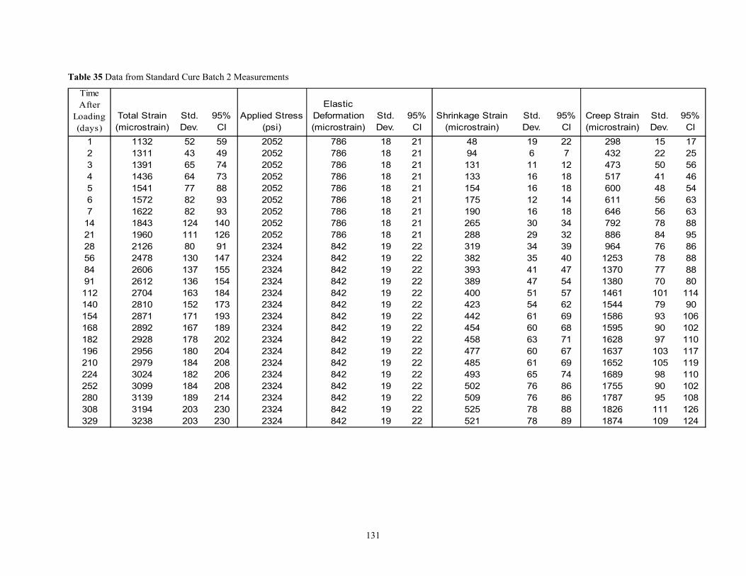
131

Table 35 Data from Standard Cure Batch 2 Measurements

TimeAfter

Loading(days)

Total Strain(microstrain)

Std.Dev.

95%CI

Applied Stress(psi)

ElasticDeformation(microstrain)

Std.Dev.

95%CI

Shrinkage Strain(microstrain)

Std.Dev.

95%CI

Creep Strain(microstrain)

Std.Dev.

95%CI

2052205220522052205220522052205220522324232423242324232423242324232423242324232423242324232423242324

101

103

9390

98

19611

97

79

485656788432

4147

19

1819

18181818

203

18181818

203189

182

180184

167178

152171

163

137136

8282124111

43656477

52

1874 124109521 8978223238 230 842 19329111 1267822 1826525 88198423194 23095 10817878619842 22 765092143139

308280

1689 11019 74493 65223024 206 84261485 11969 10519 16522979 208 842 22

477 117163767602956 19842 22204842

224

196210

106102

1628

11490

1107163458222928 202 1918260454 6819842 22 1595189289261442 69842193 15862219287154423 62842173 15442219281051400 57842184 146122192704

154168

140112

80389 54 1380 70842 221919

2612 154842

91

1616121630

382 35 40319 34288 29

39

342651819014175

224821212121

22

2122

212121

21 18154

17432 25298

2215

786786786786

786

786

842

786786786842

464150

600 54611 63

473 56517

646 63

94 7131 12

18133

792 88886 95964 8676

1253 8878147247856 13091212628 801261960211401843149316227

157261541514364139131311211321 59

4974738893

84 2606 155 22 393 1370 8847 77

1755 10290252 3099 208184 76502 86842 2219

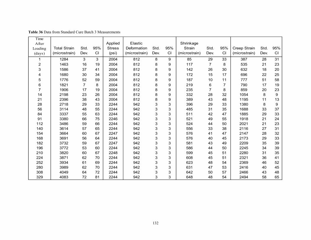
132

Table 36 Data from Standard Cure Batch 3 Measurements

TimeAfter

Loading(days)


Std.Dev.

95%CI

Applied Stress(psi)


Std.Dev.

95%CI

Shrinkage Strain

(microstrain)Std.Dev.

95%CI


Std.Dev.

95%CI

22442244

22442244

22442247

22442247

2244

22442246

2244

20042244

2004200420042004

2004200420042004

4358

404636

3431

2935

2728

21

2921

48

282118225117208

4043

3341

44

4249

151067

333

33

33

33

3

33

3

83

8888

8888

652494648 54942 334083 81329

35485 3133396 2948389 4332332 288235

1877219

3385

11

29726

9999

3

93

9999

387 31535 23

812812812812812812

942

812942

812812

632 20696 25777 58790 19859 23

117 8142 30

17172

1054 91195 13111380 981688 373355311456 48

33271828 2943239621262198141919067

182161776516804158631463212841 3

194134598

84 3337 63 942 3 511 1885 334791 3380 75 942 3 1918 24521 55

112140154168182

3486 66 942 33 524 50 2021 233614 65 942 3 556 38 2116 313664 67 942 3 576 47 2147 323691 64 942 3 576 45 2173 333732 67 942 3 2209 39581 49

196 3772 60 9422244 3 586 5044 2245 39210 3820 67 9422248 3 599 5145 2280 35224 3871 70 9422244 3 608 5145 2321 41

3934 69 942 3 623 5448 2369 523989 70 942 3 631 5347 2416 454049 72 942 3 642 5750 2466 48

252280308

3163730527172338

5566595760565953606261626472

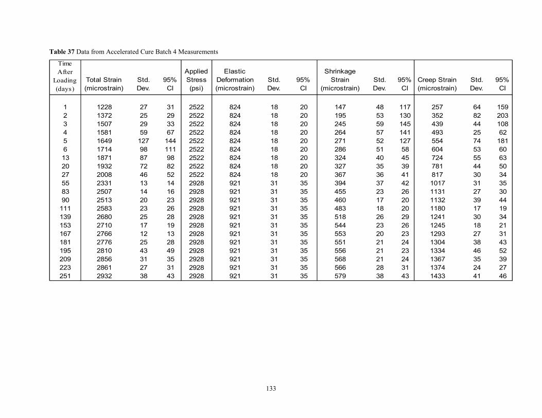
133

Table 37 Data from Accelerated Cure Batch 4 Measurements

TimeAfter

Loading(days)


Std.Dev.

95%CI

Applied Stress(psi)


Std.Dev.

95%CI

Shrinkage Strain

(microstrain)Std.Dev.

95%CI


Std.Dev.

95%CI

1433 46579 4338921 35312932 432511374 27566 3128352861 31 9211367 39568 2421352856 35 9211334 52556 2321352810 49 921

223209195

1131 3026455921 3583 2507 16

111

293367

144

31122811372215073158141649517146

981871138219322052200827 4614233155 13 1017 3531

817 3430

724 63781 5044

117130195

245 145141264

439

604 60554 181

108493 62

824824824921

824824824824824824

147 159352 20325748

53

20 127271

202020

20

35

202020

20

5828645324 4039327 3541367 3642394 37

90 2513 23 921 35 1132 44460 20111139153167

2583 26 921 3531 483 2018 11802680 28 921 3531 518 2926 12412710 19 921 3531 544 2623 12452766 13 921 3531 553 2320 1293

181 2776 28 921 35312928 551 2421 1304

1934

43

2131

27252959

127988772

1420232517122543312738

181818181818181818313131

313131

59575251

2317

64824425745355

2739173018273846352441

2522252225222522252225222522252225222928292829282928292829282928

29282928

29282928

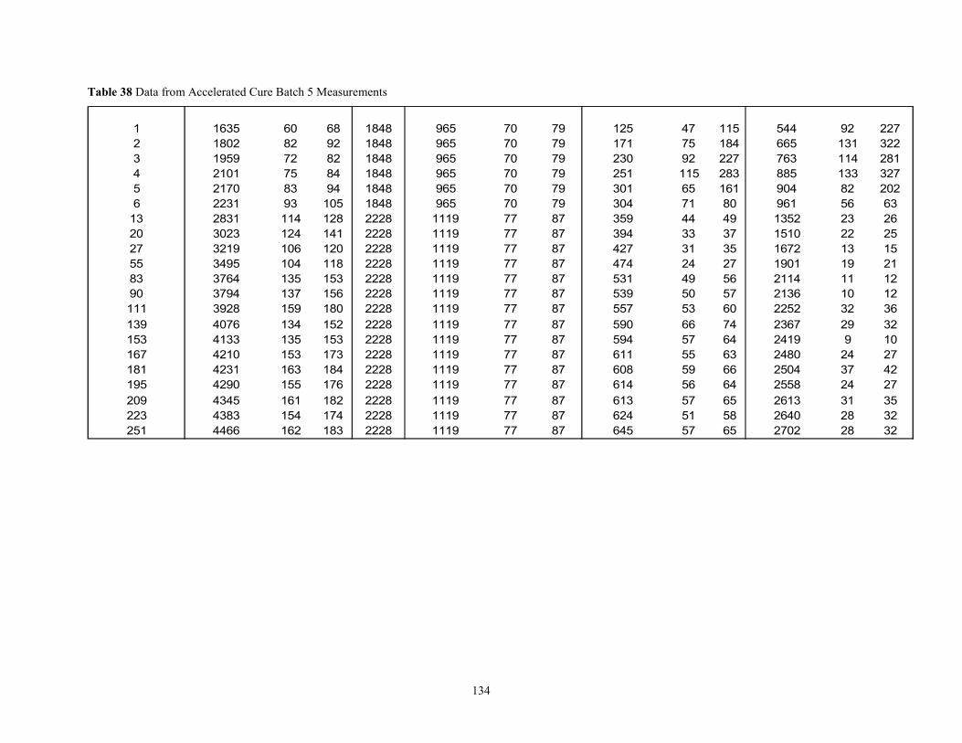
134

Table 38 Data from Accelerated Cure Batch 5 Measurements

184818481848184818481848222822282228222822282228222822282228222822282228222822282228

2640 32624 5851874383 174 11192613 35613 6557874345 182 11192558 27614 6456874290 176 1119

223209195

42

1027

2504

3632

608 66591119 87774231 1841812480611 63551119 877717342102419594 64571119 877715341332367590 74661119 877715240762252557 60531119 87771803928

153167

139111

2136 12539 571119 873794 15690

27474 2435427 313739449359

12579797979

87

8787

7987

115

8079 161301

227665 322544 92

131965965965965965965

1119

11191119

1119

763 281885 327

114133

904 202961 63

171 184230 227

283251

3041352 261510 25221672 15131901 2119118349555 104

120321927 106141302320128283113

223162170521014195931802216351 68

92828494

105

83 3764 153 1119 87 531 2114 1256

251 4466 183 1119 87 645 6557 2702 32

608272758393114124

135137159134135153163155161154162

707070707070777777777777

77777777

47759211565714433

4950

825623

111032299

24372431

2828

135

APPENDIX G

Percent Shrinkage Measurements

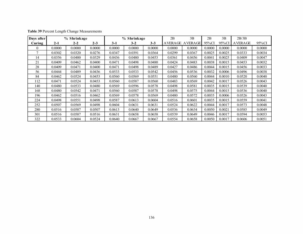
136

Table 39 Percent Length Change Measurements

Days after % Shrinkage % Shrinkage 2B 3B 2B 3B 2B/3BCuring 2-1 2-2 2-3 3-1 3-2 3-3 AVERAGE AVERAGE 95%CI 95%CI AVERAGE 95%CI

0 0.0000 0.0000 0.0000 0.0000 0.0000 0.0000 0.0000 0.0000 0.0000 0.0000 0.0000 0.00007 0.0302 0.0320 0.0276 0.0347 0.0391 0.0364 0.0299 0.0367 0.0025 0.0025 0.0333 0.003414 0.0356 0.0400 0.0329 0.0436 0.0480 0.0453 0.0361 0.0456 0.0041 0.0025 0.0409 0.004721 0.0409 0.0462 0.0400 0.0471 0.0498 0.0480 0.0424 0.0483 0.0038 0.0015 0.0453 0.003228 0.0409 0.0471 0.0400 0.0471 0.0498 0.0489 0.0427 0.0486 0.0044 0.0015 0.0456 0.003356 0.0444 0.0489 0.0436 0.0533 0.0533 0.0542 0.0456 0.0536 0.0032 0.0006 0.0496 0.003884 0.0462 0.0524 0.0453 0.0560 0.0569 0.0551 0.0480 0.0560 0.0044 0.0010 0.0520 0.0040112 0.0471 0.0524 0.0453 0.0560 0.0587 0.0560 0.0483 0.0569 0.0042 0.0017 0.0526 0.0043140 0.0480 0.0533 0.0480 0.0569 0.0596 0.0578 0.0498 0.0581 0.0035 0.0015 0.0539 0.0040168 0.0480 0.0542 0.0471 0.0560 0.0587 0.0578 0.0498 0.0575 0.0044 0.0015 0.0536 0.0040196 0.0462 0.0516 0.0462 0.0569 0.0578 0.0569 0.0480 0.0572 0.0035 0.0006 0.0526 0.0043224 0.0498 0.0551 0.0498 0.0587 0.0613 0.0604 0.0516 0.0601 0.0035 0.0015 0.0559 0.0041252 0.0507 0.0569 0.0498 0.0604 0.0631 0.0631 0.0524 0.0622 0.0044 0.0017 0.0573 0.0048280 0.0516 0.0587 0.0507 0.0613 0.0640 0.0649 0.0536 0.0634 0.0050 0.0021 0.0585 0.0049301 0.0516 0.0587 0.0516 0.0631 0.0658 0.0658 0.0539 0.0649 0.0046 0.0017 0.0594 0.0053322 0.0533 0.0604 0.0524 0.0640 0.0667 0.0667 0.0554 0.0658 0.0050 0.0017 0.0606 0.0051

137

VITA

Edward Creed Vincent was born is Charleston, West Virginia on October 3, 1977 to Frank and

Catherine Vincent. He grew up in Charleston and attended George Washington High School.

He became an Eagle Scout and an All-State musician playing tuba. He graduated high school

with honors in 1996. After high school, Ed attended Virginia Tech and completed a co-op

position with the U.S. Geological Survey. He graduated with a Bachelors of Science in Civil

Engineering in 2001. He then pursued a Master of Science degree in Civil Engineering at

Virginia Tech. Upon completion of his graduate degree in January 2003, Ed will be a structural

engineer with the US Army Corps of Engineers in Huntington, WV.

Documents

COMPRESSIVE CREEP OF A LIGHTWEIGHT, HIGH STRENGTH CONCRETE