Embed Size (px)
Citation preview
COMPRESSION OF SOCIAL NETWORKS
by
Hossein Maserrat
B.Sc., Sharif University of Technology, 1999
M.Sc., Sharif University of Technology, 2002
a Thesis submitted in partial fulfillment
of the requirements for the degree of
Doctor of Philosophy
in the
School of Computing Science
Faculty of Applied Science
c© Hossein Maserrat 2012
SIMON FRASER UNIVERSITY
Summer 2012
All rights reserved. However, in accordance with the Copyright Act of
Canada, this work may be reproduced without authorization under the
conditions for Fair Dealing. Therefore, limited reproduction of this
work for the purposes of private study, research, criticism, review and
news reporting is likely to be in accordance with the law, particularly
if cited appropriately.
APPROVAL
Name: Hossein Maserrat
Degree: Doctor of Philosophy
Title of Thesis: Compression of Social Networks
Examining Committee: Dr. Hao (Richard) Zhang
Chair
Dr. Jian Pei, Professor
Senior Supervisor
Dr. Tom Shermer, Professor
Supervisor
Dr. Binay Bhattacharya, Professor
SFU Examiner
Dr. Shen, Heng Tao, External Examiner Professor,
Information Technology & Electrical Engineering,
University of Queensland
Date Approved: July 18, 2012
ii

Partial Copyright Licence
Abstract
Compressing social networks can substantially facilitate mining and advanced analysis of
large social networks. Preferably, social networks should be compressed in a way that
they still can be queried efficiently without decompression. Arguably, neighbor queries,
which search for all neighbors of a query vertex, are the most essential operations on social
networks. In this thesis we develop a social network compression framework, which allows
efficient in-neighbor and out-neighbor query answering without replicating the data.
As a simple setting of the framework, we introduce the novel Eulerian data structure and
prove an upper bound on its bits-per-edge rate. Using the notion of k-linearization, a lossless
compression scheme is introduced as a practical compression scheme. The experiments on a
dozen real world social networks confirm the effectiveness of our design. Finally, we use our
framework to develop a lossy compresson scheme, which aims at capturing the community
structure of a given network using a predefined amount of storage. We affirmatively evaluate
the lossy compression scheme on both synthesis and real world social networks.
iii

Contents
Approval ii
Abstract iii
Contents iv
List of Tables vii
List of Figures viii
1 Introduction 1
1.1 GPSN Compression Framework . . . . . . . . . . . . . . . . . . . . . . . . . . 3
1.2 Eulerian Data Structure . . . . . . . . . . . . . . . . . . . . . . . . . . . . . . 6
1.3 Lossless Compression Scheme . . . . . . . . . . . . . . . . . . . . . . . . . . . 8
1.4 Lossy Compression Schema . . . . . . . . . . . . . . . . . . . . . . . . . . . . 10
1.5 Structure of the Thesis . . . . . . . . . . . . . . . . . . . . . . . . . . . . . . . 12
2 Related Work 13
2.1 Categorization of Related Work . . . . . . . . . . . . . . . . . . . . . . . . . . 14
2.2 The Aggregation-Based Approach . . . . . . . . . . . . . . . . . . . . . . . . . 17
2.2.1 The Virtual Node Compression Scheme . . . . . . . . . . . . . . . . . 17
2.2.2 The Summary Graph Compression Scheme . . . . . . . . . . . . . . . 18
2.2.3 Discussion . . . . . . . . . . . . . . . . . . . . . . . . . . . . . . . . . . 21
iv
2.3 Order-Based Approach . . . . . . . . . . . . . . . . . . . . . . . . . . . . . . . 24
2.3.1 WebGraph Compression Framework . . . . . . . . . . . . . . . . . . . 24
2.3.2 The Shingle Ordering Heuristic . . . . . . . . . . . . . . . . . . . . . . 27
2.3.3 Layered Label Propagation . . . . . . . . . . . . . . . . . . . . . . . . 28
2.3.4 Discussion . . . . . . . . . . . . . . . . . . . . . . . . . . . . . . . . . . 29
2.4 Clustering and Dense Subgraph Mining . . . . . . . . . . . . . . . . . . . . . 30
2.4.1 Mining Semi-Bipartite Subgraphs . . . . . . . . . . . . . . . . . . . . . 31
2.4.2 Label Propagation Clustering . . . . . . . . . . . . . . . . . . . . . . . 33
2.4.3 Structural Clustering Method . . . . . . . . . . . . . . . . . . . . . . . 36
2.4.4 Spectral Clustering . . . . . . . . . . . . . . . . . . . . . . . . . . . . . 37
2.5 The Graph Layout Problem . . . . . . . . . . . . . . . . . . . . . . . . . . . . 43
2.5.1 Definitions and Theoretical Results . . . . . . . . . . . . . . . . . . . . 43
2.5.2 Heuristics . . . . . . . . . . . . . . . . . . . . . . . . . . . . . . . . . . 47
2.6 Summary . . . . . . . . . . . . . . . . . . . . . . . . . . . . . . . . . . . . . . 49
2.7 How this thesis is related and different from the existing work . . . . . . . . . 52
3 GPSN Compression Framework 54
3.1 The GPSN Compression Framework . . . . . . . . . . . . . . . . . . . . . . . 54
3.2 Theoretical Analysis . . . . . . . . . . . . . . . . . . . . . . . . . . . . . . . . 57
3.2.1 Notions . . . . . . . . . . . . . . . . . . . . . . . . . . . . . . . . . . . 57
3.2.2 Neighbor Queries in Directed Graphs . . . . . . . . . . . . . . . . . . . 59
3.2.3 Eulerian Paths . . . . . . . . . . . . . . . . . . . . . . . . . . . . . . . 59
3.2.4 1-Linearization . . . . . . . . . . . . . . . . . . . . . . . . . . . . . . . 60
3.3 Upper Bound on Compression Rate . . . . . . . . . . . . . . . . . . . . . . . . 63
3.4 Summary . . . . . . . . . . . . . . . . . . . . . . . . . . . . . . . . . . . . . . 68
4 Lossless Compression 69
4.1 Multi Level Linearization . . . . . . . . . . . . . . . . . . . . . . . . . . . . . 69
4.2 Data Structure . . . . . . . . . . . . . . . . . . . . . . . . . . . . . . . . . . . 72
v
4.3 Compression Heuristic . . . . . . . . . . . . . . . . . . . . . . . . . . . . . . . 73
4.4 Experiments . . . . . . . . . . . . . . . . . . . . . . . . . . . . . . . . . . . . . 75
4.4.1 Experimental Setup . . . . . . . . . . . . . . . . . . . . . . . . . . . . 75
4.4.2 Comparison of the Compression Rates . . . . . . . . . . . . . . . . . . 79
4.4.3 Query Processing Time . . . . . . . . . . . . . . . . . . . . . . . . . . 80
4.4.4 Tradeoff between Local Information and Pointers . . . . . . . . . . . . 82
4.5 Summary . . . . . . . . . . . . . . . . . . . . . . . . . . . . . . . . . . . . . . 83
5 Lossy Compression 84
5.1 Overview . . . . . . . . . . . . . . . . . . . . . . . . . . . . . . . . . . . . . . 84
5.2 Graph Linearization for Lossy Compression . . . . . . . . . . . . . . . . . . . 86
5.3 Objective Function . . . . . . . . . . . . . . . . . . . . . . . . . . . . . . . . . 89
5.4 Linearization Method . . . . . . . . . . . . . . . . . . . . . . . . . . . . . . . 92
5.4.1 Connection between Parameters α and k . . . . . . . . . . . . . . . . . 93
5.4.2 A Greedy Heuristic Method . . . . . . . . . . . . . . . . . . . . . . . . 95
5.5 Empirical Evaluation . . . . . . . . . . . . . . . . . . . . . . . . . . . . . . . . 99
5.5.1 Evaluation Methodology . . . . . . . . . . . . . . . . . . . . . . . . . . 99
5.5.2 Synthesis Networks . . . . . . . . . . . . . . . . . . . . . . . . . . . . . 100
5.5.3 Centrality . . . . . . . . . . . . . . . . . . . . . . . . . . . . . . . . . . 104
5.5.4 Running Time Efficiency . . . . . . . . . . . . . . . . . . . . . . . . . 105
5.6 Summary . . . . . . . . . . . . . . . . . . . . . . . . . . . . . . . . . . . . . . 106
6 Conclusion 108
6.1 Summary . . . . . . . . . . . . . . . . . . . . . . . . . . . . . . . . . . . . . . 108
6.2 Future Work . . . . . . . . . . . . . . . . . . . . . . . . . . . . . . . . . . . . 110
Bibliography 112
vi

List of Tables
2.1 Reprinted from [8]. Naive representation using adjacency List and outdegree 26
2.2 Reprinted from [8]. Gap coding representation . . . . . . . . . . . . . . . . . 26
2.3 Reprinted from [8]. Reference coding representation . . . . . . . . . . . . . . 27
2.4 An example of a cluster of vertices passed to mining phase . . . . . . . . . . . 33
2.5 Comparison of the compression methods . . . . . . . . . . . . . . . . . . . . . 50
3.1 Comparison of compression using the Eulerian data structure against the
baseline schema. The baseline schema is the adjacency list. We presented
the ratio of the number of bits that the Eulerian data structure uses over the
number of bits that adjacency list representation uses. . . . . . . . . . . . . . 67
4.1 The dataset stats. (Acc, Gcc, and Fre are defined in Section 3.2.1) . . . . . . 75
4.2 The average number of bits per edge. The worse cases happen on those data
sets that have very poor locality measures (Gcc and Fre) . . . . . . . . . . . 80
4.3 The average access time per edge for processing adjacency queries and (in+out)
neighbor queries. . . . . . . . . . . . . . . . . . . . . . . . . . . . . . . . . . . 81
5.1 Some frequently used notions. . . . . . . . . . . . . . . . . . . . . . . . . . . . 89
5.2 Statistic of data-sets . . . . . . . . . . . . . . . . . . . . . . . . . . . . . . . . 106
vii

List of Figures
1.1 The illustration of GPSN Framework. Refer to the text for more details. . . . 4
1.2 The Eulerian data structure. The new identifiers of the nodes are illustrated. 7
2.1 Reprinted from [11]. The top graph is an example of a semi-complete bipartite
subgraph. The example illustrates the idea of aggregating a set of directed
edges by introducing a virtual node. . . . . . . . . . . . . . . . . . . . . . . . 17
2.2 Reprinted from [41]. Graph G (left) is the original graph and its compressed
representation (right). For simplicity the idea of the method is illustrated on
an undirected graph. . . . . . . . . . . . . . . . . . . . . . . . . . . . . . . . . 20
2.3 Reprinted from [11]. The prefix tree for the cluster of vertices in Table 2.4 . 34
2.4 Reprinted from [19]. A graphical illustration of a few measures for a layout ϕ. 45
2.5 Reprinted from [57]. The illustration of multi-scale framework. . . . . . . . . 50
3.1 A directed graph and its underlying undirected graph . . . . . . . . . . . . . 58
3.2 The Eulerian data structure. The new identifiers of the nodes are illustrated. 64
4.1 Multi-Level Linearization. The neighborhood scheme is {(0, 3), (9, 1)}. Arcs
point to the next appearance of the same vertex. The cells are indexed from
left to right. Position 0 is the most left cell and position 25 is the most right
cell. . . . . . . . . . . . . . . . . . . . . . . . . . . . . . . . . . . . . . . . . . 72
viii
4.2 The trade off between the bits/edge rate of local information and that of
pointers on three data sets: ca-HepPh, p2p-Gnutella24, and soc-Slashdot0902.
(K = 20, RF = 0.9) . . . . . . . . . . . . . . . . . . . . . . . . . . . . . . . . 82
4.3 The trade off between the bits/edge rate of local information and that of
pointers on three data sets: ca-HepPh, p2p-Gnutella24, and soc-Slashdot0902.
(DT = 0.25 and RF = 0.9) . . . . . . . . . . . . . . . . . . . . . . . . . . . . 83
5.1 A graph G and its lossy representation using a (3, 15)-sequence graph Gs. . . 88
5.2 The span of a path. . . . . . . . . . . . . . . . . . . . . . . . . . . . . . . . . 90
5.3 A graph G and its representation by SeqGraph data structure. . . . . . . . . 97
5.4 The bit-utility-rate of our lossy compression. . . . . . . . . . . . . . . . . . . 101
5.5 The performance of the algorithm by Clauset et al. [16] on the original net-
work, the proximity network derived from one compression, and the aggre-
gated proximity network derived from five independent compressions. . . . . . 102
5.6 The effect of (a) local range size (k) and (b) length of sequence (l). . . . . . 103
5.7 Pearson Correlation of centrality measures on original and the compressed
version . . . . . . . . . . . . . . . . . . . . . . . . . . . . . . . . . . . . . . . . 105
5.8 The running time of a single iteration of Algorithm 7. . . . . . . . . . . . . . 106
ix

Chapter 1
Introduction
Real life social networks, thanks to the popularity of World Wide Web, are getting larger
and larger, to the extent that fitting them in the main memory is a challenge. The web
graph has billions of nodes and tens of billions of edges. Facebook, as a friendship network,
has more than 900 million nodes and 125 billion edges1.
From a practical point of view, most of the social network analysis methods and al-
gorithms implicitly assume the network fits into main memory. Therefore, social network
compression indirectly addresses the scalability issues for a wide variety of algorithms.
Roughly speaking, data compression is the process of representing the data using fewer
number of bits than trivial representation. Compression is useful in practice because it
reduces the consumption of critical resources such as main memory, communication capacity,
or cache memory. A compression scheme usually exploits the statistical redundancy of the
data to achieve memory efficiency.
For example, in a text corpus, some letters statistically are more frequent than others.
Therefore, by assigning shorter codes to the frequent and longer codes to the infrequent
letters, one can obtain a better bits-per-letter cost on average. However, the statistical
redundancy often significantly depends on the characteristics of the domain of data. As a
consequence, the compression scheme has to be designed accordingly.
1http://newsroom.fb.com/content/default.aspx?NewsAreaId=22
1

CHAPTER 1. INTRODUCTION 2
On the other hand, the objective of data compression could raise a variety of require-
ments. For example, as for data archival purposes, probably the most critical measure is
the compression rate. In this case, arguably, for any future process of the archived data a
decompression phase is affordable.
As a more realistic scenario, let us assume we want to apply a pattern mining algorithm
on a dataset that does not fit into main memory. Although, a compression scheme here
could be effective for fitting the data, it has to support a number of efficient basic opera-
tions directly on the compressed version of the data depending on the requirements of the
algorithm.
Having the advances in distributed computing in mind, one might argue, by using more
computers it is always possible to fit a large network in the main memory. Although the
argument is somewhat reasonable, it raises another issue. Since the capacity of commu-
nication, in a distributed computing platform, is often the main bottleneck, an extremely
challenging problem is to partition the network so that the amount of communication be-
tween different computing units is minimum.
From this point of view, a compact representation of the network could be beneficial
not only because it reduces the number of computing units, but also it implicitly increases
the utility of the communication capacity. A compact representation often encodes the
correlated nodes (edges) together. Therefore, a better compression method potentially could
lead to a better utilization of the locality of the data.
To answer queries regarding the correlation of the nodes and edges in a social network,
an expensive link analysis usually is required. For example, given a few nodes of a network,
to find out if they belong to a dense subgraph, one has to apply an extensive link analysis
method, not only on the given vertices but also on the neighbors of them. However, poten-
tially, a compression method can provide implicit information to facilitate answering such
queries.
CHAPTER 1. INTRODUCTION 3
In order to use the existing social network analysis algorithms on a compressed net-
work, the compression framework has to often support both efficient in-neighbor 2 and
out-neighbor 3 queries. Depending on the application, we might also want to perform effi-
cient incremental updates directly on the compressed network. The focus of this dissertation
is to develop a compression framework for social networks that addresses these additional
requirements. We refer to such a compression framework as a General Purpose Social Net-
work (GPSN) compression framework. To the best of our knowledge there is no compression
method for social network in the literature that qualifies as a GPSN compression framework.
For the rest of this chapter, we present a high level overview of the major results of
the dissertation. In Section 1.1, we illustrate the core idea for the General Purpose Social
Network (GPSN) compression framework. Section 1.2 discusses an upper-bound on bits-
per-edge rate for a simple setting of the framework, which we refer to it as Eulerain data
structure. In Sections 1.3 and 1.4 we review two lossless and lossy compression schemes,
respectively.
1.1 GPSN Compression Framework
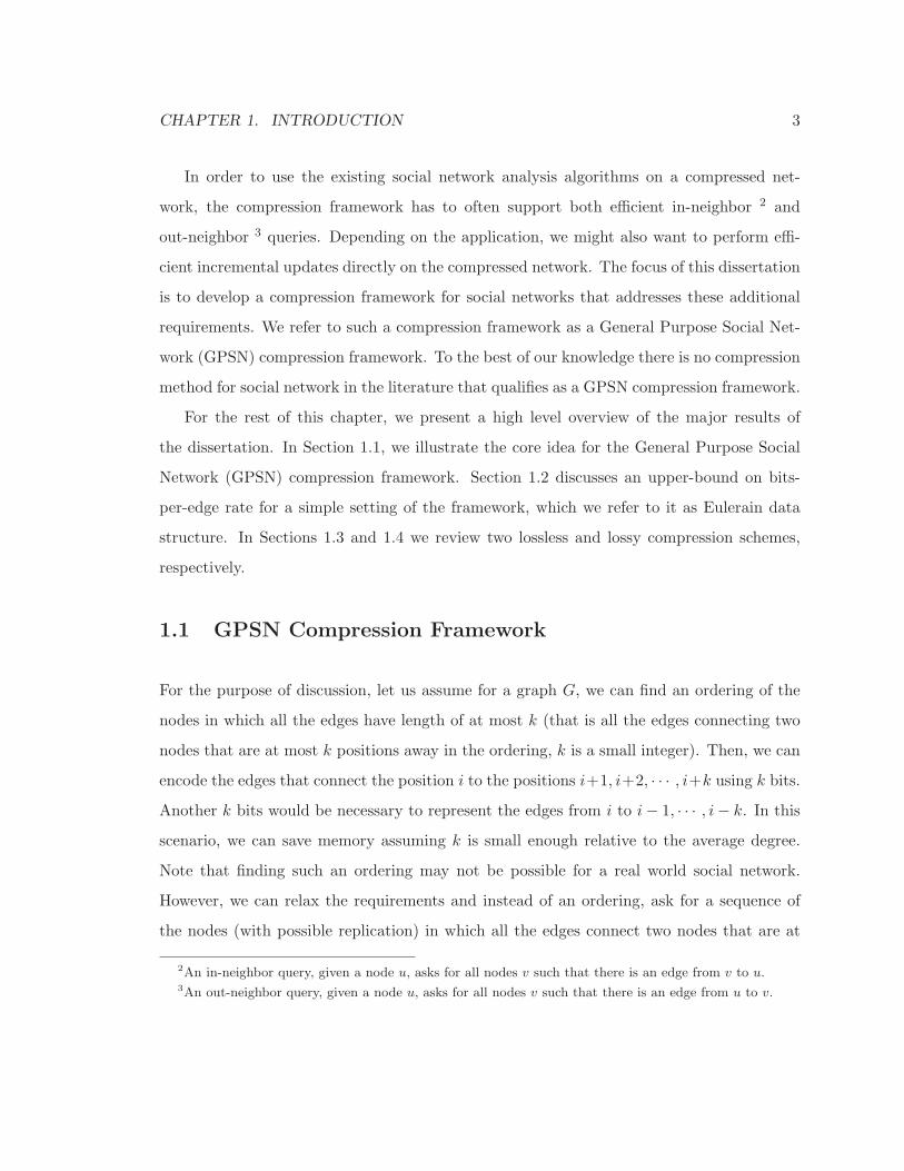
For the purpose of discussion, let us assume for a graph G, we can find an ordering of the
nodes in which all the edges have length of at most k (that is all the edges connecting two
nodes that are at most k positions away in the ordering, k is a small integer). Then, we can
encode the edges that connect the position i to the positions i+1, i+2, · · · , i+k using k bits.
Another k bits would be necessary to represent the edges from i to i− 1, · · · , i− k. In this
scenario, we can save memory assuming k is small enough relative to the average degree.
Note that finding such an ordering may not be possible for a real world social network.
However, we can relax the requirements and instead of an ordering, ask for a sequence of
the nodes (with possible replication) in which all the edges connect two nodes that are at
2An in-neighbor query, given a node u, asks for all nodes v such that there is an edge from v to u.3An out-neighbor query, given a node u, asks for all nodes v such that there is an edge from u to v.
CHAPTER 1. INTRODUCTION 4
���� ���� ���� ������ �� �� ���� ����v1 v2 v3 v4 v5 v6 v7 v8 v9
(a) Graph G
v7 v8 v7 v6 v5 v4 v1 v2 v1v8 v9 v6 v5 v4 v3 v2 v6 v3
01 01 11 11 01 00 1110 00 10 00 11 00 0001 11 1010
(b) A representation of G using a sequence of nodes in which all theedges connect two nodes next to each other.
00 01 01 10 01 00 01 10 11 00 11 11 00 10 01 10 10 0001 11
v6v7v8v9 v5 v4 v3 v2 v1 v6
(c) A representation of G using a sequence of nodes in which all theedges connect two nodes at most two positions away.
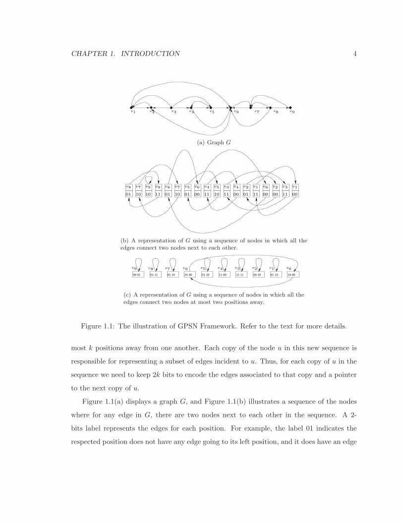
Figure 1.1: The illustration of GPSN Framework. Refer to the text for more details.
most k positions away from one another. Each copy of the node u in this new sequence is
responsible for representing a subset of edges incident to u. Thus, for each copy of u in the
sequence we need to keep 2k bits to encode the edges associated to that copy and a pointer
to the next copy of u.
Figure 1.1(a) displays a graph G, and Figure 1.1(b) illustrates a sequence of the nodes
where for any edge in G, there are two nodes next to each other in the sequence. A 2-
bits label represents the edges for each position. For example, the label 01 indicates the
respected position does not have any edge going to its left position, and it does have an edge
CHAPTER 1. INTRODUCTION 5
going to its right node. The arcs are pointers to the next copy of the same node. Figure
1.1(c) illustrates a sequence in which the maximum length of all edges is 2. The 4-bits labels
inside the box encode the edges and the arcs are pointers to the next copy of the same node.
If there is only one copy of the node in the sequence, the pointer points to itself.
Let us assume we can find a sequence S of length l, in which all the edges are connecting
two nodes at most k positions away from one another. In such a case, the network can
be represented using exactly l × (2k + ⌈log2 l⌉) bits; we need ⌈log2 l⌉ to encode the next
pointer and 2k bits to encode the associated edges for each position. This framework has
several benefits. First, similar to the order-based methods it reduces the social network
compression to an elegant combinatorial problem. Second, it allows efficient incremental
updates, in-neighbor and out-neighbor queries. Third, intuitively in the sequence S, we
expect the nodes that belong to a dense subgraph appear close to each other, and if a node
is part of several (overlapping) dense subgraphs, the node would appear several times in the
sequence.
To have a solid compression scheme within the GPSN framework, we need to develop two
modules: (1) a linearization algorithm/heuristic that given a network, outputs a sequence
of the nodes, and (2) an encoding protocol to encode the edges associated to each position
of the sequence.
As an example, we will formulate a trivial representation schema using the principles
of GPSN framework. Let us assume that the linearization algorithm enumerates all the
edges in arbitrary order, and represents each edge by its source and destination. This would
produce a sequence of length 2|E| of the nodes. Then, precisely there is one edge associated
to each position; each edge connects a position with an even index to its next position.
Therefore, the parity of the index of the positions is enough to recover the edges of the
network. The representation scheme merely stores a pointer to the next appearance of the
same node for each position. In total, the scheme uses exactly 2|E|(⌈log2(|E|)⌉ + 1) bits.
Note that, this is comparable to the adjacency list representation where each node stores
both lists of incoming and outgoing edges.
CHAPTER 1. INTRODUCTION 6
Note that to be able to compare the results with previous work in the literature, similar
to [8, 9, 14], we assume: (1) It is possible to assign new identifiers to the vertices. (2) The
data structure is not responsible for maintaining the mapping between the old and new iden-
tifiers. (3) Finally, there are no labels for edges. Please note that we can straightforwardly
extend the data structure to remove the above assumptions.
Contribution. We introduce the novel GPSN compression framework. Our method for
compressing social networks, comparing to the state-of-the-art methods, has the advantage
of supporting efficient in-neighbor4, out-neighbor queries5, and incremental updates6. The
GPSN framework exploits a sequence S, in which the nodes that belong to a dense subgraph
of a given network, appears in proximate positions to achieve compression.
1.2 Eulerian Data Structure
A k-linearization of a given graph G is a sequence of nodes in which all the edges have a
length at most k. In Chapter 3, we show that finding the optimal 1-linearization is possible
in linear time. Note that any graph would have an optimal 1-linearization regardless of
the existence of the Eulerian path. Constructing such a linearization is, in fact, equivalent
to decomposing the graph into the minimum number of edge-disjoint paths such that each
edge appears exactly once in one of the paths. However, the problem of finding an optimal
k-linearization, when k is given as part of the input, is NP-Hard.
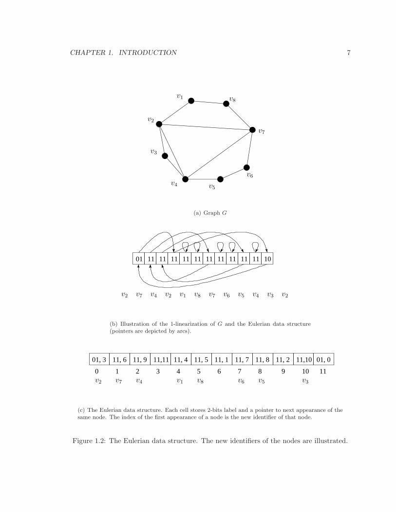
The Eulerian data structure for a graph G stores an optimal 1-linearization L of G
using an array of the same length as L. Let v(i) be the vertex in G that appears at the
position i of L. For the cell i of the array, we keep the following two pieces of information:
(1) Edge Information: two bits specifying if edges (v(i− 1), v(i)) and (v(i), v(i− 1)) belong
to e(G), respectively. (2) Pointer: a pointer to the next appearance of v(i), if this is the
4Given the node v in a graph G, in-neighbor query asks for all the nodes u such that (u, v) be an edge G5Given the node v in a graph G, out-neighbor query asks for all the nodes u such that (v, u) be an edge
G6Incremental update is the operation of applying the changes directly on the compressed version of the
graph
CHAPTER 1. INTRODUCTION 7
v3
v5
v6
v7
v8v1
v2
v4
(a) Graph G
01 11 11 11 11 11 11 11 11 11 1011
v2 v2 v2v7 v4 v1 v8 v7 v6 v5 v4 v3
(b) Illustration of the 1-linearization of G and the Eulerian data structure(pointers are depicted by arcs).
01, 3 11, 6 11, 9 11,11 11, 4 11, 5 11, 1 11, 7 11, 8 11, 2 11,10 01, 0
0 1 2 3 4 5 6 7 8 9 10 11v2 v7 v4 v1 v8 v6 v5 v3
(c) The Eulerian data structure. Each cell stores 2-bits label and a pointer to next appearance of thesame node. The index of the first appearance of a node is the new identifier of that node.
Figure 1.2: The Eulerian data structure. The new identifiers of the nodes are illustrated.
CHAPTER 1. INTRODUCTION 8
last appearance of v(i), then the pointer points to the first appearance of the vertex.
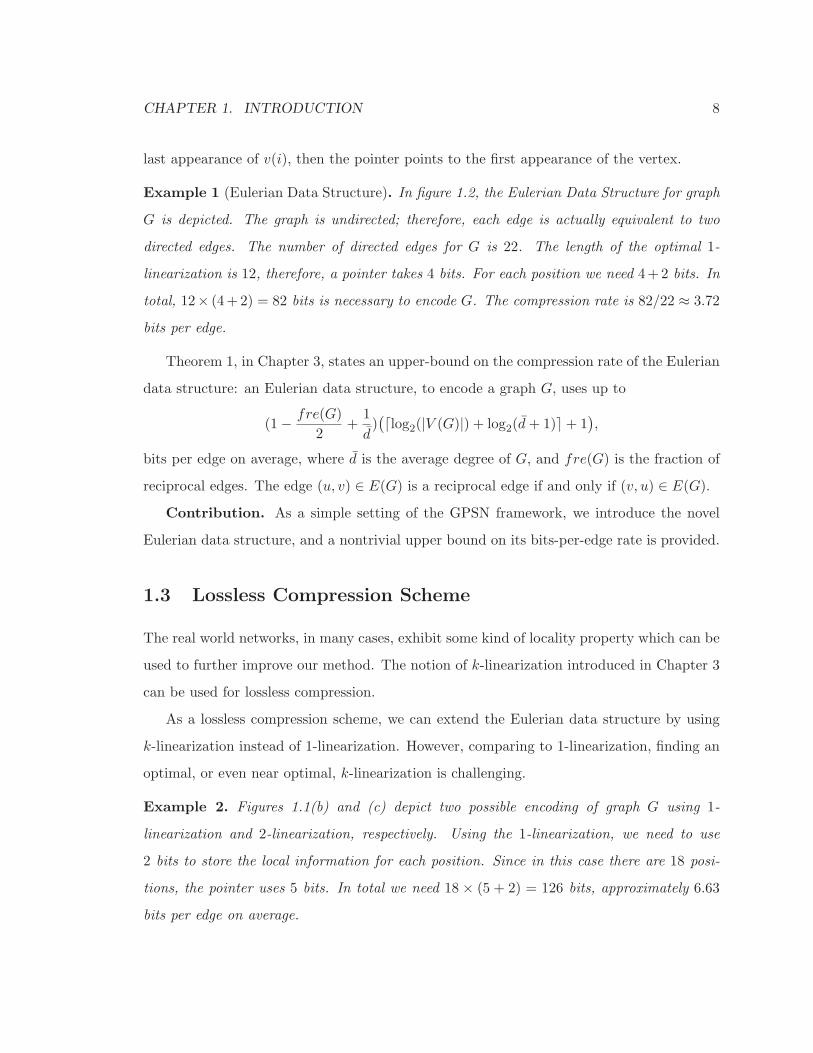
Example 1 (Eulerian Data Structure). In figure 1.2, the Eulerian Data Structure for graph
G is depicted. The graph is undirected; therefore, each edge is actually equivalent to two
directed edges. The number of directed edges for G is 22. The length of the optimal 1-
linearization is 12, therefore, a pointer takes 4 bits. For each position we need 4+2 bits. In
total, 12× (4+2) = 82 bits is necessary to encode G. The compression rate is 82/22 ≈ 3.72
bits per edge.
Theorem 1, in Chapter 3, states an upper-bound on the compression rate of the Eulerian
data structure: an Eulerian data structure, to encode a graph G, uses up to
(1− fre(G)
2+
1
d)(
⌈log2(|V (G)|) + log2(d+ 1)⌉+ 1)
,
bits per edge on average, where d is the average degree of G, and fre(G) is the fraction of
reciprocal edges. The edge (u, v) ∈ E(G) is a reciprocal edge if and only if (v, u) ∈ E(G).
Contribution. As a simple setting of the GPSN framework, we introduce the novel
Eulerian data structure, and a nontrivial upper bound on its bits-per-edge rate is provided.
1.3 Lossless Compression Scheme
The real world networks, in many cases, exhibit some kind of locality property which can be
used to further improve our method. The notion of k-linearization introduced in Chapter 3
can be used for lossless compression.
As a lossless compression scheme, we can extend the Eulerian data structure by using
k-linearization instead of 1-linearization. However, comparing to 1-linearization, finding an
optimal, or even near optimal, k-linearization is challenging.
Example 2. Figures 1.1(b) and (c) depict two possible encoding of graph G using 1-
linearization and 2-linearization, respectively. Using the 1-linearization, we need to use
2 bits to store the local information for each position. Since in this case there are 18 posi-
tions, the pointer uses 5 bits. In total we need 18 × (5 + 2) = 126 bits, approximately 6.63
bits per edge on average.
CHAPTER 1. INTRODUCTION 9
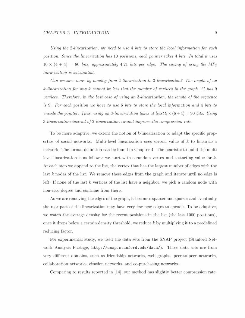
Using the 2-linearization, we need to use 4 bits to store the local information for each
position. Since the linearization has 10 positions, each pointer takes 4 bits. In total it uses
10 × (4 + 4) = 80 bits, approximately 4.21 bits per edge. The saving of using the MP2
linearization is substantial.
Can we save more by moving from 2-linearization to 3-linearization? The length of an
k-linearization for any k cannot be less that the number of vertices in the graph. G has 9
vertices. Therefore, in the best case of using an 3-linearization, the length of the sequence
is 9. For each position we have to use 6 bits to store the local information and 4 bits to
encode the pointer. Thus, using an 3-linearization takes at least 9× (6+4) = 90 bits. Using
3-linearization instead of 2-linearization cannot improve the compression rate.
To be more adaptive, we extent the notion of k-linearization to adapt the specific prop-
erties of social networks. Multi-level linearization uses several value of k to linearize a
network. The formal definition can be found in Chapter 4. The heuristic to build the multi
level linearization is as follows: we start with a random vertex and a starting value for k.
At each step we append to the list, the vertex that has the largest number of edges with the
last k nodes of the list. We remove these edges from the graph and iterate until no edge is
left. If none of the last k vertices of the list have a neighbor, we pick a random node with
non-zero degree and continue from there.
As we are removing the edges of the graph, it becomes sparser and sparser and eventually
the rear part of the linearization may have very few new edges to encode. To be adaptive,
we watch the average density for the recent positions in the list (the last 1000 positions),
once it drops below a certain density threshold, we reduce k by multiplying it to a predefined
reducing factor.
For experimental study, we used the data sets from the SNAP project (Stanford Net-
work Analysis Package, http://snap.stanford.edu/data/). These data sets are from
very different domains, such as friendship networks, web graphs, peer-to-peer networks,
collaboration networks, citation networks, and co-purchasing networks.
Comparing to results reported in [14], our method has slightly better compression rate.
CHAPTER 1. INTRODUCTION 10
However, the real advantage of our lossless compression comes from the ability of answering
both in-neighbor and out-neighbor queries without replicating the data. More experimental
results are provided in Chapter 4.
Contribution. The lossless compression scheme is a practical setting of the GPSN
framework, in which a notion of multi-level linearization is utilized. We introduce a greedy
heuristic to build a “good” multi-level linearization for a given graph. An extensive set of
experiments validate our design.
1.4 Lossy Compression Schema
Although, there are a few pioneering studies on social network compression, they only focus
on lossless approaches. In Chapter 5, we tackle the novel problem of lossy compression
of social networks. The trade-off between memory and “information-preserved” in a lossy
compression presents an interesting angle for social network analysis, and at the same time
makes the problem very challenging. We propose a lossy graph compression approach,
based on our GPSN framework. We do so by designing an objective function to measure
the quality of a given linearization with the respect of community structure of the network.
We present an interesting and practically effective greedy algorithm to optimize such an
objective function. Our experimental results on both real data sets and synthetic data
sets demonstrate the promise of our method. However, there is no theoretical analysis to
guarantee the performance of our heuristic.
From the practical point of view, the noise edges and vertices in large social networks
do not help in analysis of the network. Instead, they may compromise the quality of social
network analysis. An appropriate lossy compression of a social network can discard the noise
edges and vertices in the network. Consequently, the lossy compression may be presented
as a higher quality input for social network analysis. In other words, lossy compression of
social networks can serve as a preprocessing step in social network analysis. This goes far
beyond just saving space. The experimental study in Chapter 5 verifies our claim.
The idea of representing the edges of a network by a sequence of vertices naturally
CHAPTER 1. INTRODUCTION 11
inspires a lossy compression scheme. To explain such a scheme, a dual definition of k-
linearization could prove to be useful. The definition of k-covered edges is presented in
Section 5.3. The intuition is as follows: a subset A ⊆ E(G) is k-covered by a sequence S of
the nodes of a given graph G, if for all e ∈ A, the length of e according to S is less than or
equal to k. Ek(S) would be the largest set that is k-covered by S.
The setting for the lossy compression problem is as follows: given two parameters k
and l, find a sequence S of nodes with length l such that Ek(S) captures the community
structure of the network. Since communities are the building blocks of a social network,
such a scheme would cover the majority of the edges of the network assuming reasonable
values for k and l.
We design an objective function to measure how well a given sequence S captures the
community structure of a social network. A critical issue would be to design such an
objective function that is sensitive to the loss of community structure. Instead of developing
a utility function parameterized by k, we consider a utility function that optimizes for edges
of short spans in the corresponding sequence S. For this purpose, we introduce a parameter
α (0 < α < 1) that controls the preference for shorter spans. We build the connection
between parameter α and parameter k in Section 5.4. The objective function is as follows:
f(S,G) =∑
1≤i≤length(S)
(∑
e∈Ei
αspan(e))2, (1.1)
where Ei is the set of edges associated to the position i of the sequence S, and span(e) is
the stretch of edge e according to sequence S. Sections 5.3 and 5.4 discuss the objective
function and the reasoning behind it in details.
A critical question is that what would the lost of information in lossy compression scheme
do to the community structure of the network. A set of experiments introduced in Section
5.5 aims to evaluate the effect of lossy compression on the community structure of the
network. Chapter 5 provides detailed results on real world and synthesis networks.
Contribution. Our lossy compression scheme is designed to capture the global com-
munity structure of social networks using a predefined amount of storage. We introduce an
objective function which quantifies how well a sequence S captures the community structure

CHAPTER 1. INTRODUCTION 12
of a given network. Our objective function turns the problem of lossy compression to an
optimization problem. For optimizing such an objective function we develop a local search
heuristic. Finally, we evaluate our method on both synthesis and real world networks.
1.5 Structure of the Thesis
In this chapter, we provide a high level and intuitive introduction of the core idea of the
GPSN compression framework. Chapter 2 reviews the related work. Then, we justify the
design of our GPSN framework by mentioning three solid compression schemes, designed
base on the principles of this framework. The first scheme, the Eulerian data structure, is
one of the simplest settings for which the framework is not trivial. The simplicity in this case
allows us to prove a theoretical upper-bound on the compression rate. The detailed proof of
the upper bound can be found in Chapter 3. A lossless compression scheme is discussed in
details in Chapter 4. For the third and last study, we present an overview of the design of
the lossy compression scheme. Chapter 5 discusses the lossy compression scheme in details.
We conclude the thesis in Chapter 6.
Chapter 2
Related Work
In the last decade, World Wide Web [3] has been the focus of much research, both from
academic and industrial perspectives. Among other things, it has been a diverse and incred-
ibly huge source of data. Particularly, it is rich with different types of social networks. In
this thesis, a social network is a graph which models the binary relations among a certain
set of objects. The nodes of the graph represent objects and the edges represent the binary
relations. Often, relations come from a social phenomenon. A binary relation could be a
one way or two ways relation.
For example, in a friendship network, a node is a person and an undirected edge is
representing the friendship between two persons. The web graph is an abstraction for the
web pages (URLs) and the hyper links among them. The nodes are representing web pages.
There is a directed edge from web page x to web page y, if there is a hyper link from x to y.
Likewise, a collaboration network typically models a set of individuals and the collaborative
relationship among them.
Social networks have been exploited in many different applications, such as search en-
gines, epidemic analysis for diseases, modeling information and behaviour cascades [45, 21].
However, the huge amount of information always comes with the scalability challenges,
in both time and memory aspects. In this chapter, we focus on the literature related to
compression of social networks.
13
CHAPTER 2. RELATED WORK 14
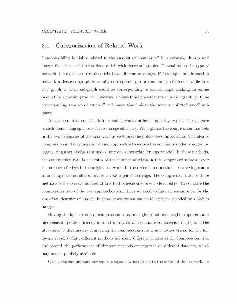
2.1 Categorization of Related Work
Compressibility is highly related to the amount of “regularity” in a network. It is a well
known fact that social networks are rich with dense subgraphs. Depending on the type of
network, these dense subgraphs might have different meanings. For example, in a friendship
network a dense subgraph is usually corresponding to a community of friends, while in a
web graph, a dense subgraph could be corresponding to several pages making an online
manual for a certain product. Likewise, a dense bipartite subgraph in a web graph could be
corresponding to a set of “survey” web pages that link to the same set of “reference” web
pages.
All the compression methods for social networks, at least implicitly, exploit the existence
of such dense subgraphs to achieve storage efficiency. We organize the compression methods
in the two categories of the aggregation-based and the order-based approaches. The idea of
compression in the aggregation-based approach is to reduce the number of nodes or edges, by
aggregating a set of edges (or nodes) into one super-edge (or super-node). In these methods,
the compression rate is the ratio of the number of edges in the compressed network over
the number of edges in the original network. In the order-based methods, the saving comes
from using fewer number of bits to encode a particular edge. The compression rate for these
methods is the average number of bits that is necessary to encode an edge. To compare the
compression rate of the two approaches sometimes we need to have an assumption for the
size of an identifier of a node. In those cases, we assume an identifier is encoded by a 32-bits
integer.
Having the four criteria of compression rate, in-neighbor and out-neighbor queries, and
incremental update efficiency in mind we review and compare compression methods in the
literature. Unfortunately comparing the compression rate is not always trivial for the fol-
lowing reasons: first, different methods are using different criteria as the compression rate,
and second, the performance of different methods are reported on different datasets, which
may not be publicly available.
Often, the compression method reassigns new identifiers to the nodes of the network. In
CHAPTER 2. RELATED WORK 15
the scenarios that the original identifiers are informative, storing a two-way mapping from
the original identifiers to the new ones is necessary. Consistent with the literature [41, 8, 14],
to evaluate the compression rate we ignore the cost of this mapping. This is a reasonable
assumption because the size of such a mapping is proportional to the number of nodes, and
the number of nodes is often much smaller compared to the number of edges. As the last
remark, all the compression methods that we describe in this thesis assume the input is a
simple directed graph (i.e., a directed graph without multiple edges).
We categorize the literature related to the compression methods in the following four
categories:
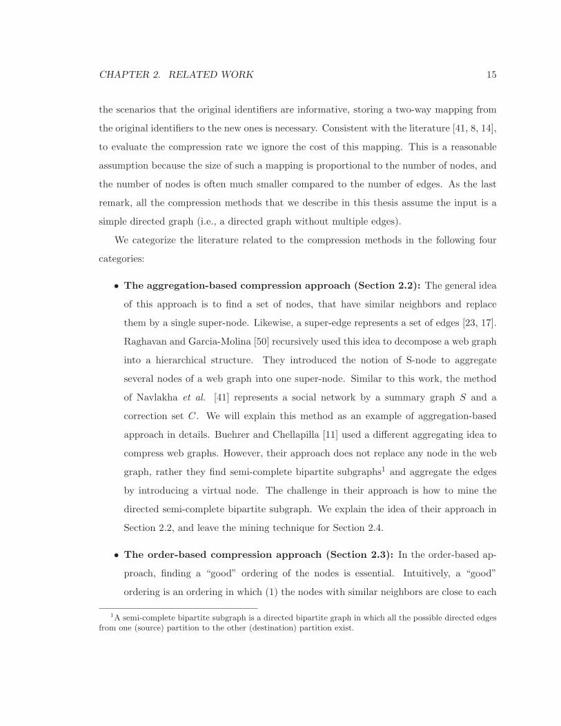
• The aggregation-based compression approach (Section 2.2): The general idea
of this approach is to find a set of nodes, that have similar neighbors and replace
them by a single super-node. Likewise, a super-edge represents a set of edges [23, 17].
Raghavan and Garcia-Molina [50] recursively used this idea to decompose a web graph
into a hierarchical structure. They introduced the notion of S-node to aggregate
several nodes of a web graph into one super-node. Similar to this work, the method
of Navlakha et al. [41] represents a social network by a summary graph S and a
correction set C. We will explain this method as an example of aggregation-based
approach in details. Buehrer and Chellapilla [11] used a different aggregating idea to
compress web graphs. However, their approach does not replace any node in the web
graph, rather they find semi-complete bipartite subgraphs1 and aggregate the edges
by introducing a virtual node. The challenge in their approach is how to mine the
directed semi-complete bipartite subgraph. We explain the idea of their approach in
Section 2.2, and leave the mining technique for Section 2.4.
• The order-based compression approach (Section 2.3): In the order-based ap-
proach, finding a “good” ordering of the nodes is essential. Intuitively, a “good”
ordering is an ordering in which (1) the nodes with similar neighbors are close to each
1A semi-complete bipartite subgraph is a directed bipartite graph in which all the possible directed edgesfrom one (source) partition to the other (destination) partition exist.
CHAPTER 2. RELATED WORK 16
other, and (2) the nodes that belong to a dense subgraph, fall in proximate positions
[8, 6, 7]. The existing order-based methods either use external information to establish
the ordering (e.g. lexical ordering of URLs) or they rely on a heuristic to produce it.
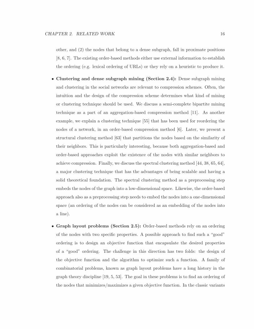
• Clustering and dense subgraph mining (Section 2.4): Dense subgraph mining
and clustering in the social networks are relevant to compression schemes. Often, the
intuition and the design of the compression scheme determines what kind of mining
or clustering technique should be used. We discuss a semi-complete bipartite mining
technique as a part of an aggregation-based compression method [11]. As another
example, we explain a clustering technique [55] that has been used for reordering the
nodes of a network, in an order-based compression method [6]. Later, we present a
structural clustering method [63] that partitions the nodes based on the similarity of
their neighbors. This is particularly interesting, because both aggregation-based and
order-based approaches exploit the existence of the nodes with similar neighbors to
achieve compression. Finally, we discuss the spectral clustering method [44, 38, 65, 64],
a major clustering technique that has the advantages of being scalable and having a
solid theoretical foundation. The spectral clustering method as a preprocessing step
embeds the nodes of the graph into a low-dimensional space. Likewise, the order-based
approach also as a preprocessing step needs to embed the nodes into a one-dimensional
space (an ordering of the nodes can be considered as an embedding of the nodes into
a line).
• Graph layout problems (Section 2.5): Order-based methods rely on an ordering
of the nodes with two specific properties. A possible approach to find such a “good”
ordering is to design an objective function that encapsulate the desired properties
of a “good” ordering. The challenge in this direction has two folds: the design of
the objective function and the algorithm to optimize such a function. A family of
combinatorial problems, known as graph layout problems have a long history in the
graph theory discipline [19, 5, 53]. The goal in these problems is to find an ordering of
the nodes that minimizes/maximizes a given objective function. In the classic variants
CHAPTER 2. RELATED WORK 17
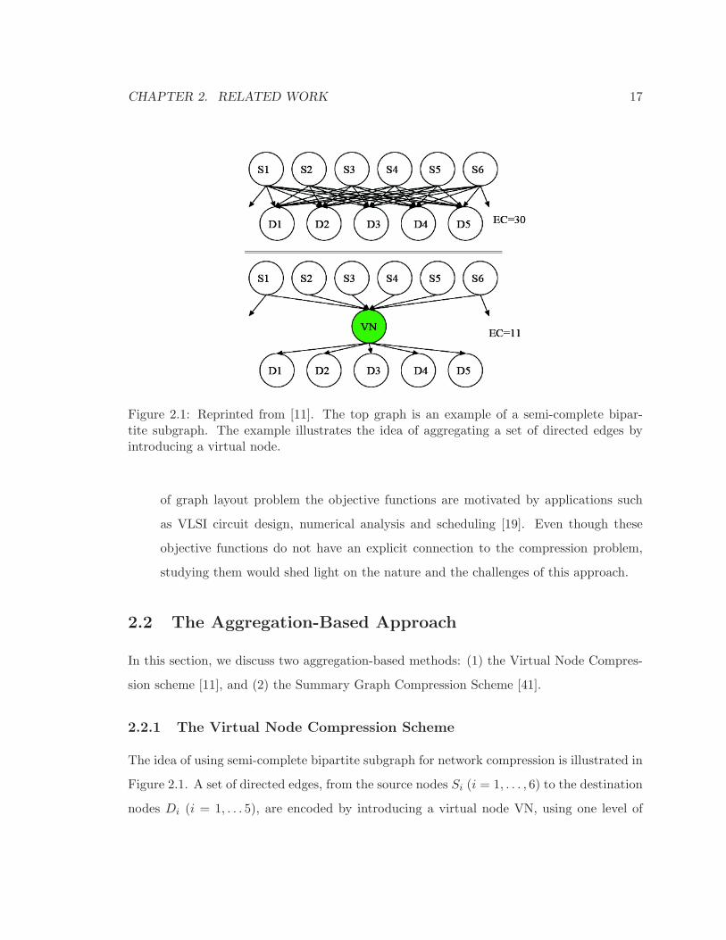
Figure 2.1: Reprinted from [11]. The top graph is an example of a semi-complete bipar-tite subgraph. The example illustrates the idea of aggregating a set of directed edges byintroducing a virtual node.
of graph layout problem the objective functions are motivated by applications such
as VLSI circuit design, numerical analysis and scheduling [19]. Even though these
objective functions do not have an explicit connection to the compression problem,
studying them would shed light on the nature and the challenges of this approach.
2.2 The Aggregation-Based Approach
In this section, we discuss two aggregation-based methods: (1) the Virtual Node Compres-
sion scheme [11], and (2) the Summary Graph Compression Scheme [41].
2.2.1 The Virtual Node Compression Scheme
The idea of using semi-complete bipartite subgraph for network compression is illustrated in
Figure 2.1. A set of directed edges, from the source nodes Si (i = 1, . . . , 6) to the destination
nodes Di (i = 1, . . . 5), are encoded by introducing a virtual node VN, using one level of
CHAPTER 2. RELATED WORK 18
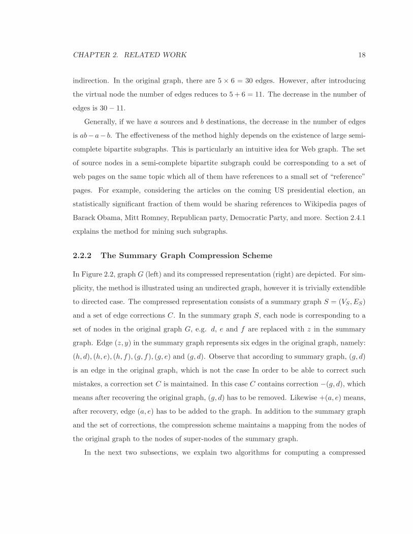
indirection. In the original graph, there are 5 × 6 = 30 edges. However, after introducing
the virtual node the number of edges reduces to 5 + 6 = 11. The decrease in the number of
edges is 30− 11.
Generally, if we have a sources and b destinations, the decrease in the number of edges
is ab−a− b. The effectiveness of the method highly depends on the existence of large semi-
complete bipartite subgraphs. This is particularly an intuitive idea for Web graph. The set
of source nodes in a semi-complete bipartite subgraph could be corresponding to a set of
web pages on the same topic which all of them have references to a small set of “reference”
pages. For example, considering the articles on the coming US presidential election, an
statistically significant fraction of them would be sharing references to Wikipedia pages of
Barack Obama, Mitt Romney, Republican party, Democratic Party, and more. Section 2.4.1
explains the method for mining such subgraphs.
2.2.2 The Summary Graph Compression Scheme
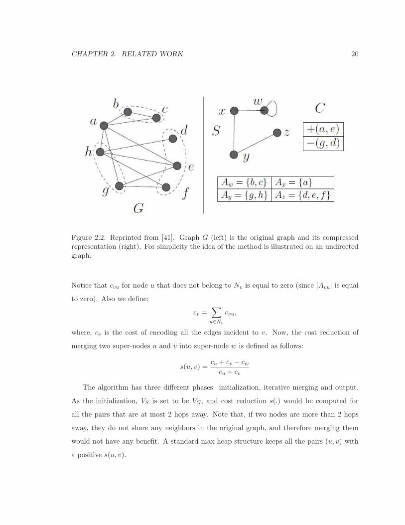
In Figure 2.2, graph G (left) and its compressed representation (right) are depicted. For sim-
plicity, the method is illustrated using an undirected graph, however it is trivially extendible
to directed case. The compressed representation consists of a summary graph S = (VS , ES)
and a set of edge corrections C. In the summary graph S, each node is corresponding to a
set of nodes in the original graph G, e.g. d, e and f are replaced with z in the summary
graph. Edge (z, y) in the summary graph represents six edges in the original graph, namely:
(h, d), (h, e), (h, f), (g, f), (g, e) and (g, d). Observe that according to summary graph, (g, d)
is an edge in the original graph, which is not the case In order to be able to correct such
mistakes, a correction set C is maintained. In this case C contains correction −(g, d), whichmeans after recovering the original graph, (g, d) has to be removed. Likewise +(a, e) means,
after recovery, edge (a, e) has to be added to the graph. In addition to the summary graph
and the set of corrections, the compression scheme maintains a mapping from the nodes of
the original graph to the nodes of super-nodes of the summary graph.
In the next two subsections, we explain two algorithms for computing a compressed
CHAPTER 2. RELATED WORK 19
representation (S,C), where S is a summary graph and C is a set of corrections. The
objective is to find a representation (S,C) such that the sum of |ES | + |C| is minimized.
Before explaining the algorithms, notice that the edge set ES and the correction set C can
be optimally determined based on the super-nodes in VS .
Assuming VS is fixed, we show how to compute ES and C. Let v and u be two super-
nodes in VS . We define Πuv as the set of all pairs (a, b) such that a ∈ Au and b ∈ Av, where
Au and Av are the two set of nodes in the original graph, that are replaced by super-nodes
u and v, respectively. Observe that some of the pairs in Πuv might not be an edge in the
original graph. Let Auv ⊆ Πuv be the set of all those pairs that are also an edge of the
original graph. Now, for encoding the edges in Auv there are two possibilities: (1) add (u, v)
to the summary graph ES and Πuv − Auv to the correction set C with the negative sign.
(2) add Auv to C with the positive sign. The cost would be |Πuv| − |Auv|+1 for the former
case, and |Auv| in the case of latter. Therefore, one must add the super-edge (u, v) if and
only if |Auv| > (|Πuv|+ 1)/2. Then, the corrections have to be chosen accordingly. We can
conclude that the task here is to find a good partitioning of the nodes in the original graph
into super-nodes.
The Greedy Algorithm
The greedy algorithm starts with having each node of the original graph as a super-node
(VS = VG). Then, iteratively it tries to merge the super-nodes, based on a cost reduction
function s(u, v), until no improvement is possible. We define a neighborhood Nv for each
super-node v as follows:
Nv = {u ∈ VS |∃a ∈ Av ∧ ∃b ∈ Au → (a, b) ∈ EG}
In other words, u is in neighborhood of v if and only if for some node a ∈ Av and b ∈ Au,
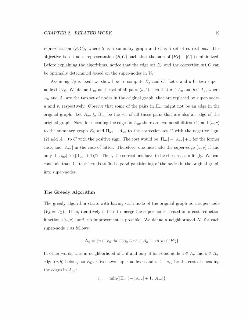
edge (a, b) belongs to EG. Given two super-nodes u and v, let cvu be the cost of encoding
the edges in Auv:
cvu = min{|Πuv| − |Auv|+ 1, |Auv|}
CHAPTER 2. RELATED WORK 20
Figure 2.2: Reprinted from [41]. Graph G (left) is the original graph and its compressedrepresentation (right). For simplicity the idea of the method is illustrated on an undirectedgraph.
Notice that cvu for node u that does not belong to Nv is equal to zero (since |Avu| is equalto zero). Also we define:
cv =∑
u∈Nv
cvu,
where, cv is the cost of encoding all the edges incident to v. Now, the cost reduction of
merging two super-nodes u and v into super-node w is defined as follows:
s(u, v) =cu + cv − cwcu + cv
The algorithm has three different phases: initialization, iterative merging and output.
As the initialization, VS is set to be VG, and cost reduction s(.) would be computed for
all the pairs that are at most 2 hops away. Note that, if two nodes are more than 2 hops
away, they do not share any neighbors in the original graph, and therefore merging them
would not have any benefit. A standard max heap structure keeps all the pairs (u, v) with
a positive s(u, v).
CHAPTER 2. RELATED WORK 21
During the merging phase, iteratively the pair (x, y) with maximum s(.) is chosen. Then,
the super-nodes x and y have to be removed from VS , and merged into the super-node w.
Finally, w has to be added to VS . Notice that as a side effect of the merging operation the
value of s(.) for some pairs might change. Precisely, those pairs that contain x, y or any
neighbor of them have to be considered for cost reduction revaluation. Algorithm 1 is the
pseudo code for this heuristic.
The Randomized Algorithm
Since recomputing the cost reduction function for all the affected pairs of super-nodes in
each step of greedy algorithm is expensive, the randomized algorithm is proposed to reduce
the time complexity. Similar to greedy algorithm, the heuristic initializes VS to VG. Then, it
iteratively merge nodes to form the final set of super-nodes. These super-nodes are divided
into two categories, unfinished (U) and finished (F). The algorithm starts with all nodes in
the U category, and ends when all the nodes are in the F category.
In each iteration a node u, uniformly at random, is chosen from the U category. The
reduction cost of this node with respect to all nodes in its 2 hop neighborhood is computed.
Let v be the node such that s(v, u) is the largest. If merging u and v gives a positive
reduction, they should be merged into super-node w, otherwise we add u to the F category.
Algorithm 2 is the pseudo code for the randomized heuristic.
2.2.3 Discussion
The Virtual Node scheme uses an adjacency list table to store the compressed graph, there-
fore incremental updates and out-neighbor queries are efficient. However, the in-neighbor
queries are not efficient, without replicating the data. Also, since the method uses a fast
heuristic for mining the semi-complete bipartite subgraph, it is scalable. A disadvantage
of the method is that the effectiveness, from the compression-rate point of view, depends
on the existence of semi-complete bipartite subgraphs. As it is clear from the experiments
in [11], web graphs tend to have relatively large semi-complete bipartite subgraphs. The

CHAPTER 2. RELATED WORK 22
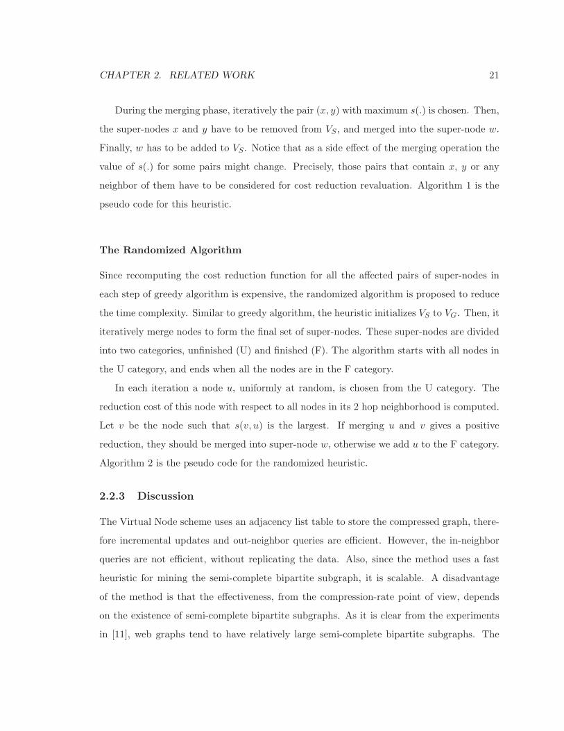
Algorithm 1 Reprinted from [41]. The pseudo code for three phases of greedy algorithmfor computing the summarization graph GS and correction set C. The algorithm consistedof three phases: Initialization, Iterative merging and Output.
/*Initialization phase*/VS = VG; H = {};for all u, v ∈ VS that are 2 hops apart doif s(u, v) > 0 theninsert (u, v, s(u, v)) into H;
end ifend for/*Iterative merging phase*/while H 6= {} doChoose pair (u, v) ∈ H with the largest s(u, v) value;w = u ∪ v; /* merge super-nodes u and v */VS = VS − {u, v} ∪ {w};for all x ∈ VS that are within 2 hops of u or v doDelete (u, x) and (v, x) from H;if s(w, x) > 0 theninsert (w, x, s(w, x)) into H;
end ifend forfor all x, y ∈ VS such that x or y is in Nw doDelete (x, y) from H;if s(x, y) > 0 theninsert (x, y, s(x, y)) into H;
end ifend for
end while/*Output phase*/ES = C = {};for all u, v ∈ VS doif |Auv| > (|Πuv|+ 1)/2 thenAdd (u, v) to ES ;Add −(a, b) to C for all (a, b) ∈ Πuv −Auv;
elseAdd +(a, b) to C for all (a, b) ∈ Auv;
end ifend forreturn representation R = (S = (VS , ES), C);
CHAPTER 2. RELATED WORK 23
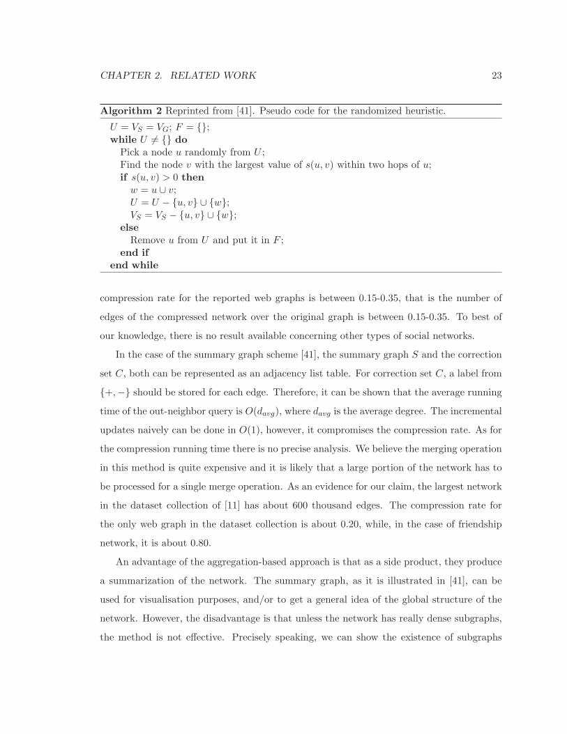
Algorithm 2 Reprinted from [41]. Pseudo code for the randomized heuristic.
U = VS = VG; F = {};while U 6= {} doPick a node u randomly from U ;Find the node v with the largest value of s(u, v) within two hops of u;if s(u, v) > 0 thenw = u ∪ v;U = U − {u, v} ∪ {w};VS = VS − {u, v} ∪ {w};
elseRemove u from U and put it in F ;
end ifend while
compression rate for the reported web graphs is between 0.15-0.35, that is the number of
edges of the compressed network over the original graph is between 0.15-0.35. To best of
our knowledge, there is no result available concerning other types of social networks.
In the case of the summary graph scheme [41], the summary graph S and the correction
set C, both can be represented as an adjacency list table. For correction set C, a label from
{+,−} should be stored for each edge. Therefore, it can be shown that the average running
time of the out-neighbor query is O(davg), where davg is the average degree. The incremental
updates naively can be done in O(1), however, it compromises the compression rate. As for
the compression running time there is no precise analysis. We believe the merging operation
in this method is quite expensive and it is likely that a large portion of the network has to
be processed for a single merge operation. As an evidence for our claim, the largest network
in the dataset collection of [11] has about 600 thousand edges. The compression rate for
the only web graph in the dataset collection is about 0.20, while, in the case of friendship
network, it is about 0.80.
An advantage of the aggregation-based approach is that as a side product, they produce
a summarization of the network. The summary graph, as it is illustrated in [41], can be
used for visualisation purposes, and/or to get a general idea of the global structure of the
network. However, the disadvantage is that unless the network has really dense subgraphs,
the method is not effective. Precisely speaking, we can show the existence of subgraphs

CHAPTER 2. RELATED WORK 24
with a density strictly higher than 1/2 is necessary, and for substantial saving we need a
density close to one. Comparing the performances of the two compression methods could
be informative. First, the excellent compression rate of Virtual Node scheme suggests that
the web graphs have relatively large semi-complete bipartite subgraphs. We believe, this is
the reason that the summary graph scheme also works well on the web graphs. At the same
time, the poor performance of the summary graph scheme on the friendship networks is an
evidence for the lack of relatively large very dense subgraphs.
2.3 Order-Based Approach
Methods in this category rely on a particular ordering of the nodes in which similar nodes,
i.e., nodes with the similar set of neighbors, fall in the proximate positions. The ordering
might come as an external information [8], or is computed using the link analysis of the
graph [14, 6]. In either case, the ordering should have the following two properties:
• Closeness Similarity: the proximate nodes tend to have similar neighbors.
• Edge Locality: the edges of the graph tend to connect a pair of “close by” nodes.
Next, we explain the major ideas of the WebGraph framework [8, 6, 7, 14] that exploits the
lexicographical ordering of the URLs to achieve impressive compression rate on web graphs.
It is also worth mentioning that WebGraph uses and improves ideas from the Connectivity
Server [4] and the LINK database [52].
2.3.1 WebGraph Compression Framework
There are two critical components for the WebGraph framework:
• ζ codes [9]: this is a family of codes, particularly designed for storing integers that
come from a power law distribution2 in a certain exponent range. Unlike fixed length
2A power law distribution is a distribution whose density function (mass function in the discrete case)p(x) is proportional to Lx−α, where L is a constant and α is the exponent.
CHAPTER 2. RELATED WORK 25
code, the length of the code to represent a given number x depends on the value of x. A
ζ code to represent a number x would use at most 2⌈log2(x)⌉ bits. The unary encoding
of a number x is x−1 zeros, followed by a one. The general idea for these codes can be
explained as follows: for a given number x, first we write unary encoding of ⌈log2(x)⌉,followed by ⌈log2(x)⌉ bits encoding number x. However, we have to mention this is
only to demonstrate the general idea, while the actual encoding is more complicated.
The key observation is that most integers coming from a power law distribution are
small numbers, therefore this approach on average would use fewer number of bits,
comparing to the fixed length codes.
• The compression format [8]: the framework uses the adjacency list table (e.g. table
2.1) of a network as the starting point. The rows of the adjacency table is ordered lex-
icographically based on the URLs of the web pages. Then, by exploiting the closeness
similarity of the nodes, and the application of ζ codes, an impressive storage efficiency
is achievable.
The details of ζ codes are out of scope for this report, and can be found in [8]. However,
we will discuss the major ideas of the compression format for the rest of this subsection.
Naive Representation [8]: The naive representation is an adjacency list table, in which
the nodes are ordered according to the lexicographic order of the corresponding URLs. The
adjacency list for each node is preceded with the out degree of the node. Also the list is
sorted in the increasing order. Table 2.1 is an example of the naive representation.
Gap coding [8]: the advantage of the sorted out-neighbor list in the naive representa-
tion is that the gaps between consecutive out-links are going to follow a pattern. In fact,
experimentally it is shown that they follow a power low distribution [8]. To exploit this
observation, instead of storing the adjacency list, one can represent the out-neighbors by
storing the gap list. For a given node x let S(x) = (s1, s2, · · · , sk) be the adjacency list, then,
instead one can store the gap list: g(x) = (s1−x, s2− s1− 1, s3− s2− 1, · · · , sk− sk−1− 1).

CHAPTER 2. RELATED WORK 26
Node Outdegree Out-neighbors
· · · · · · · · ·15 11 13, 15, 16, 17, 18, 19, 23, 24, 203, 315, 103416 10 15, 16, 17, 22, 23, 24, 315, 316, 317, 304117 018 5 13, 15, 16, 17, 50· · · · · · · · ·
Table 2.1: Reprinted from [8]. Naive representation using adjacency List and outdegree
Table 2.2: Reprinted from [8]. Gap coding representation
Node Outdegree Out-neighbors
· · · · · · · · ·15 11 3, 1, 0, 0, 0, 0, 3, 0, 178, 111, 71816 10 1, 0, 0, 4, 0, 0, 290, 0, 0, 272317 018 5 9, 1, 0, 0, 32· · · · · · · · ·
Note that, since the adjacency list S(x) is sorted, except possibly for the first one, all
these numbers would be non-negative. To eliminate this exception, one can handle the first
number as a special case. The first number in the list would be encoded using the following
bijective mapping:
ν(x) =
2x if x ≥ 0
2|x| − 1 if x < 0
Table 2.2 illustrates the gap coding technique.
Reference Coding [8]: the reference coding technique exploits the similarity between
the adjacency lists of the proximate positions in the lexicographic order. The idea is that
instead of representing S(x) directly, one can represent it as a modified version of another
list S(y). Where, y is a node, or equivalently a row of the adjacency table, that appears
before x. We call S(y) the reference list, and x − y the reference number. To encode S(x)
with respect to S(y), both the reference number and a vector of bits of length |S(y)| have
CHAPTER 2. RELATED WORK 27
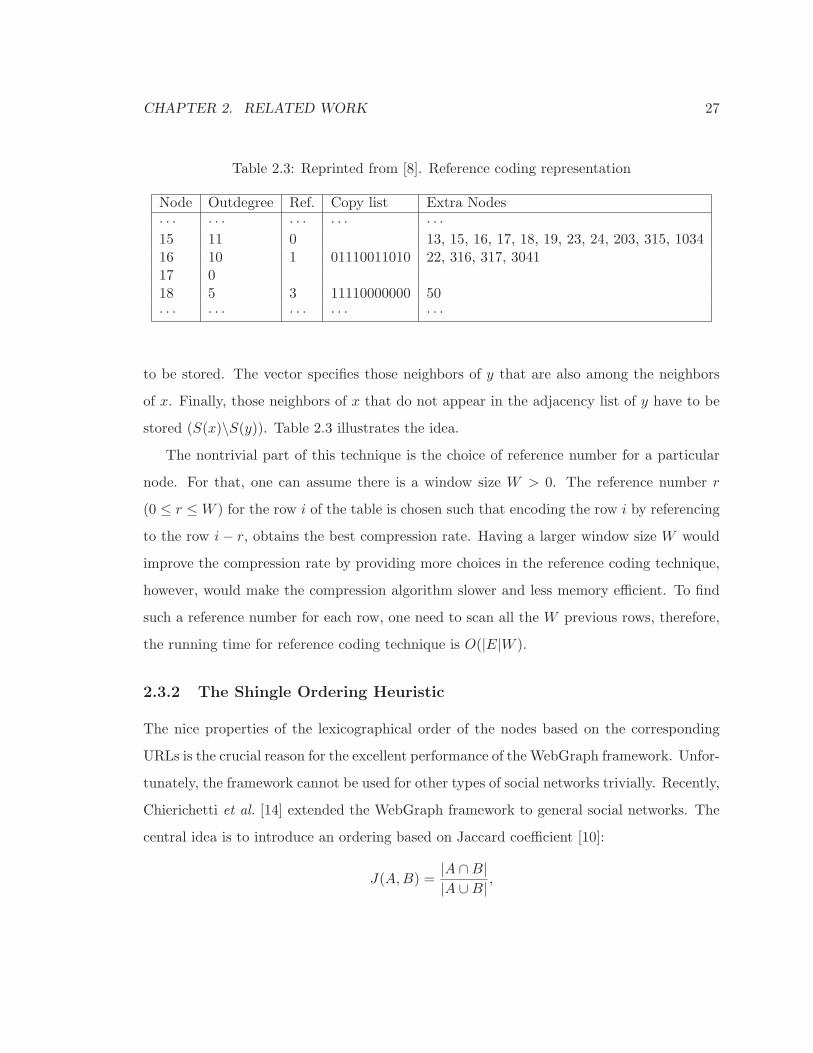
Table 2.3: Reprinted from [8]. Reference coding representation
Node Outdegree Ref. Copy list Extra Nodes
· · · · · · · · · · · · · · ·15 11 0 13, 15, 16, 17, 18, 19, 23, 24, 203, 315, 103416 10 1 01110011010 22, 316, 317, 304117 018 5 3 11110000000 50· · · · · · · · · · · · · · ·
to be stored. The vector specifies those neighbors of y that are also among the neighbors
of x. Finally, those neighbors of x that do not appear in the adjacency list of y have to be
stored (S(x)\S(y)). Table 2.3 illustrates the idea.
The nontrivial part of this technique is the choice of reference number for a particular
node. For that, one can assume there is a window size W > 0. The reference number r
(0 ≤ r ≤W ) for the row i of the table is chosen such that encoding the row i by referencing
to the row i− r, obtains the best compression rate. Having a larger window size W would
improve the compression rate by providing more choices in the reference coding technique,
however, would make the compression algorithm slower and less memory efficient. To find
such a reference number for each row, one need to scan all the W previous rows, therefore,
the running time for reference coding technique is O(|E|W ).
2.3.2 The Shingle Ordering Heuristic
The nice properties of the lexicographical order of the nodes based on the corresponding
URLs is the crucial reason for the excellent performance of the WebGraph framework. Unfor-
tunately, the framework cannot be used for other types of social networks trivially. Recently,
Chierichetti et al. [14] extended the WebGraph framework to general social networks. The
central idea is to introduce an ordering based on Jaccard coefficient [10]:
J(A,B) =|A ∩B||A ∪B| ,

CHAPTER 2. RELATED WORK 28
where A and B are two sets. Jaccard coefficient is a similarity measure for two sets A and
B. Shingle ordering is a heuristic based on this notion. Let S(x) and S(y) be the sets of
neighbors for x and y, respectively. Let σ be a random permutation of the nodes of the
network. Then, for node x:
Mσ(x) = σ−1(mina∈S(x){σ(a)})
Intuitively,Mσ(x) is the neighbor of x that appears first among all other neighbors according
to σ. We call Mσ(x) the shingle of x. It is easy to prove the following:
Pr[Mσ(x) =Mσ(y)] =|S(x) ∩ S(y)||S(x) ∪ S(y)| = J(S(x), S(y))
The shingle ordering heuristic sorts the nodes based on their shingle. The idea is that if
the neighbors of two nodes highly overlap, there is a good chance that they both have the
same shingle, therefore it is likely that they will be close to each other. For breaking the
ties a second (and third ...) shingle can be used.
2.3.3 Layered Label Propagation
Very recently, Vigna et al. [6] introduced the Layered Label Propagation (LLP) algorithm
for reordering the nodes of a graph, and showed that using the output of this algorithm
the compression rate of WebGraph framework can be improved, for both web graphs and
social networks. It is worth mentioning, the layered label propagation algorithm in essence
is a clustering method built up on the work of [51, 56]. The LLP algorithm uses a variant
of label propagation algorithms, known as Absolute Pott Model (APM), as a subroutine.
APM has a parameter γ as an input and guarantees that the resulting clusters have the
density at least γ/(γ+1). The value of γ in this algorithm is related to the resolution level of
the resulting clusters. For values close to zero the algorithm returns fewer, sparser clusters.
As γ increases the clusters become smaller and denser. More details on this algorithm is
provided in Section 2.4.2.
The intuitive description of the LLP algorithm is as follows: we run the APM clus-
tering algorithm with k different parameters γ1, γ2, · · · , γk. Let λi be the label of node v
CHAPTER 2. RELATED WORK 29
corresponding to parameter γi. We assign the tuple (λ1, · · · , λk) to v as a label. Then, we
sort the nodes lexicographically based on this label. Although, there is no discussion in [6]
regarding the value of k, presumably it is the smallest number that resolves (almost) all
the ties in the lexicographic order. The parameter γi is chosen uniformly at random from
{2−i|i = 0, · · · l} ∪ 0, where l is a fixed constant. We should mention that the intuition
behind this choice is unclear for us and there is no discussion provided by the authors [6].
2.3.4 Discussion
The average neighborhood query time for the WebGraph framework is O(Cdavg), where C
is the limit on the length of the reference chains and davg is the average degree. Since C is a
predefined small constant number, the neighborhood query time on average is O(davg). The
framework does not allow sub linear incremental updates and in-neighbors query answering.
Assuming the order of the nodes is provided, the compression time is O(|E|W ). The
running time to build the lexicographic order is O(|V |log|V |), however, the time to build
the shingle order depends on the number of edges as well (O(|V |log|V |+ |E|)). The runningtime of LLP algorithm is proportional to |E|1.3 [54]3.
Similar to the aggregation-based approach the compression rate of the order-based ap-
proach on web graphs is extremely good, while for other types of social networks the per-
formance is quite poor. The compression rate for order-based approach is measured by
the average number of bits that is necessary to represent a single edge. The WebGraph
framework uses 2-4 bits/edge to encode a typical web graph. However, when the framework
is coupled with the shingle ordering heuristic, the compression rate for other type of social
networks is in the range of 10-15 bits/edge [14]. Also the order that is produced by the
LLP algorithm comparing to both the shingle heuristic ordering and lexicographic ordering
in most cases can improve the compression rate by up to 25 percent [6].
3However, this running time is based on experimental analysis, rather than analytical analysis. That iswhy we do not use the big O notation for this case.
CHAPTER 2. RELATED WORK 30
2.4 Clustering and Dense Subgraph Mining
Any compression method, at least implicitly, exploits the existence of the dense subgraphs
of a given social network in order to achieve compression. This naturally brings the topic
of dense subgraph mining and clustering into picture. Clustering in the social networks is a
broad and diverse area.
The techniques and algorithms in this area very much depend on the problem formu-
lation. An early study formulate the problem as a min-max problem. The min-max cut
method [20] partitions the nodes of a graph into clusters C1, · · · , Ck such that it minimizes
the number of edges between different clusters, and maximizes the number of edges inside
the clusters. Later, the notion of modularity is proposed to measure the quality of a clus-
tering [43], and a fast greedy algorithm to optimize it was proposed in [16]. The SCAN
algorithm [63] introduced as a extension of the popular DBSCAN algorithm [22] to the
social networks. A comprehensive survey on the clustering method can be found here [27].
Dense subgraph mining also is studied extensively. A recent work [61] introduces a mapping
technique that maps edges and nodes to a multi-dimensional space in which dense areas are
corresponding to dense subgraphs. Furthermore, many papers studied the problem of dense
subgraph mining specific to the web graph [30, 26, 34]. The goal here is not to cover all
the aspects of clustering and dense subgraph mining, rather we explain a few methods that
have clear connections to the existing compression schemes.
In this section, we explain a dense subgraph mining method that successfully has been
used in a compression framework. A clustering method known as Absolute Pott Model,
which has been used for reordering the nodes of a network in the WebGraph framework,
is discussed. In addition, we explain a structural clustering algorithm (SCAN), which uses
the similarity between the neighborhood of the nodes as a measure for partitioning the
nodes. Since both order-based and aggregation-based approaches use the same notion of
neighbors similarity to achieve compression, we believe structural clustering potentially
can be beneficial. Finally, we consider the spectral clustering method. Spectral clustering
particularly is interesting, because as a preprocessing step it uses an embedding of the nodes
CHAPTER 2. RELATED WORK 31
to a low-dimensional space. Note that, the ordering of the nodes in the order based methods
can be considered as an embedding to the one-dimensional space.
2.4.1 Mining Semi-Bipartite Subgraphs
In this section, we explain a mining technique for finding a set of source nodes that all
share a set of destination nodes as out neighbors (the top graph in Figure 2.1 displays an
example). As we described in Section 2.2.1, this particular subgraph exploits by the Virtual
Node scheme to achieve compression. The mining of this type of bipartite subgraph can
be seen as a frequent itemset mining problem, where the out-neighbors of each vertex is a
transaction. Items are corresponding to the vertices of the graph. Then, the goal is to find
those sets of items that appeared in at least m transactions. The parameter m is called the
minimum support. The number of transactions and the number of items are both equal to
the number of vertices in the graph. The full enumeration of those patterns is particularly
challenging, because in our setting the minimum support is 2 (since an itemset with support
of 2 could be benefical for purpose of compression). However, in our setting there is no need
to recall all such frequent itemsets.
The mining method relies on a two phases heuristic: a clustering phase, in which the
vertices are clustered based on their similarity, i.e., Jaccard coefficient of their neighbor set.
Next, in a pattern mining phase, the frequent patterns are discovered using the fast frequent
itemset mining method introduced in [12].
Phase 1: Clustering
The clustering method uses k independent shingles for each vertex (see section 2.3.1 for the
definition of the shingle). These shingles can be considered as k independent samples from
the out-neighbors of each vertex. Therefore, if the out-neighbors of two vertices u and v
highly overlap, it is likely that the sets of shingles of u and v also highly overlap. Note that,
k is a small fixed number.
The clustering algorithm is as follows: first, we obtain a table in which the rows are the
CHAPTER 2. RELATED WORK 32
vertices and the columns are the shingles. Then, we sort the rows of the table based on
the lexicographic ordering of the shingle vectors. We traverse across the table to cluster the
rows with the same shingle together, starting from column one. If the size of a cluster is
larger than a threshold we move to the next shingle and refine the cluster to smaller parts.
We continue this until the size of all clusters are less than the threshold, or we reach to the
last shingle. Note that, this method biases the left-most shingle.
Phase 2: Pattern Mining
The objective of the pattern mining phase is to find common subsets of neighbors of a given
cluster of vertices. Pattern P is a subset of vertices of the network. The frequency of P
is the number of those vertices v ∈ C, that have all the vertices in P as a neighbor. The
compression performance of P is defined as follows (see section 2.2.1):
Compression(P ) = freq(P )|P | − |P | − freq(P ) (2.1)
The idea of the pattern mining phase is to first reorder the out-neighbor list of the nodes
such that the vertex Ids with higher frequency sort first. Then, one can treat the out-
neighbor lists as string. The out-neighbor lists would be added to a prefix tree one by one4.
Each node in the tree is associated with a vertex Id as the label. The prefix of the node t
in the tree is the sequence of vertex Ids, starting from the root, and along the path to t.
Table 2.4 is a toy example of a typical cluster of vertices, passed to mining phase. The
vertex Ids in the out-neighbor list are sorted according to their frequency. Figure 2.3 is
illustrating the corresponding prefix tree. Note that, before adding the out-neighbor list
to the tree, we remove the vertices with frequency one. Each node of the tree, in addition
of its label, is associated with a list of transactions, i.e., out-neighbor lists, that share the
prefix of the node. We refer to the vertices in this list as the support vertices of the node.
4A prefix tree (or a trie) is a data structure to store a set of strings. In prefix tree, the nodes are labeledwith letters, then the string associated with each node is the sequence of labels, starting from the root, alongthe path to that node. All the descendants of a node have a common prefix of the string associated withthat node, and the root is usually associated with the empty string. Values are normally not associated withevery node, only with leaves and some inner nodes that correspond to keys of interest.

CHAPTER 2. RELATED WORK 33
Vertex Id Out-neighbor List
23 1,2,3,5,6,10,12,15
55 1,2,3,5
102 1,2,3,20
204 1,7,8,9
13 1,2,3,8
64 1,2,3,5,6,10,12,15
43 1,2,3,5,6,10,22,31
431 1,2,3,5,6,10,21,31,67
Table 2.4: An example of a cluster of vertices passed to mining phase
For example, there are two nodes in the prefix tree (Figure 2.3) with label 8. The prefix
sequence of the first one is 1, 8 and second one is 1, 2, 3, 8. The out-neighbor sequence of the
vertex 204 is the only sequence that supports 1, 8 (after removing 7 which has frequency 1),
while the out-neighbor sequence of vertex 13 supports 1, 2, 3, 8.
The merit of using the prefix tree is that it suggests a heuristic approach to exploit the
trade off between the size and the frequency of candidate patterns. The prefix associated
with each node of the prefix tree, could be a potential pattern. For leaf t of the tree, the size
of the prefix of t is large, however, the frequency of the prefix is small. As we move towards
the root from t, the size of prefix decreases and the frequency increases. The algorithm in
one scan of the prefix tree, generates those patterns with high compression performance.
Then, it sorts the patterns based on their compression performance and replace the edges
for each pattern with a virtual node (see section 2.2.1) starting from the top of the list.
More details of the mining algorithm can be found here [12].
2.4.2 Label Propagation Clustering
The label propagation algorithms are a family of algorithms that share the following idea:
at the beginning of the algorithm each node has a unique label. During each round, every
node would update its label according to a predefined rule. The algorithm terminates as
soon as no update is possible.
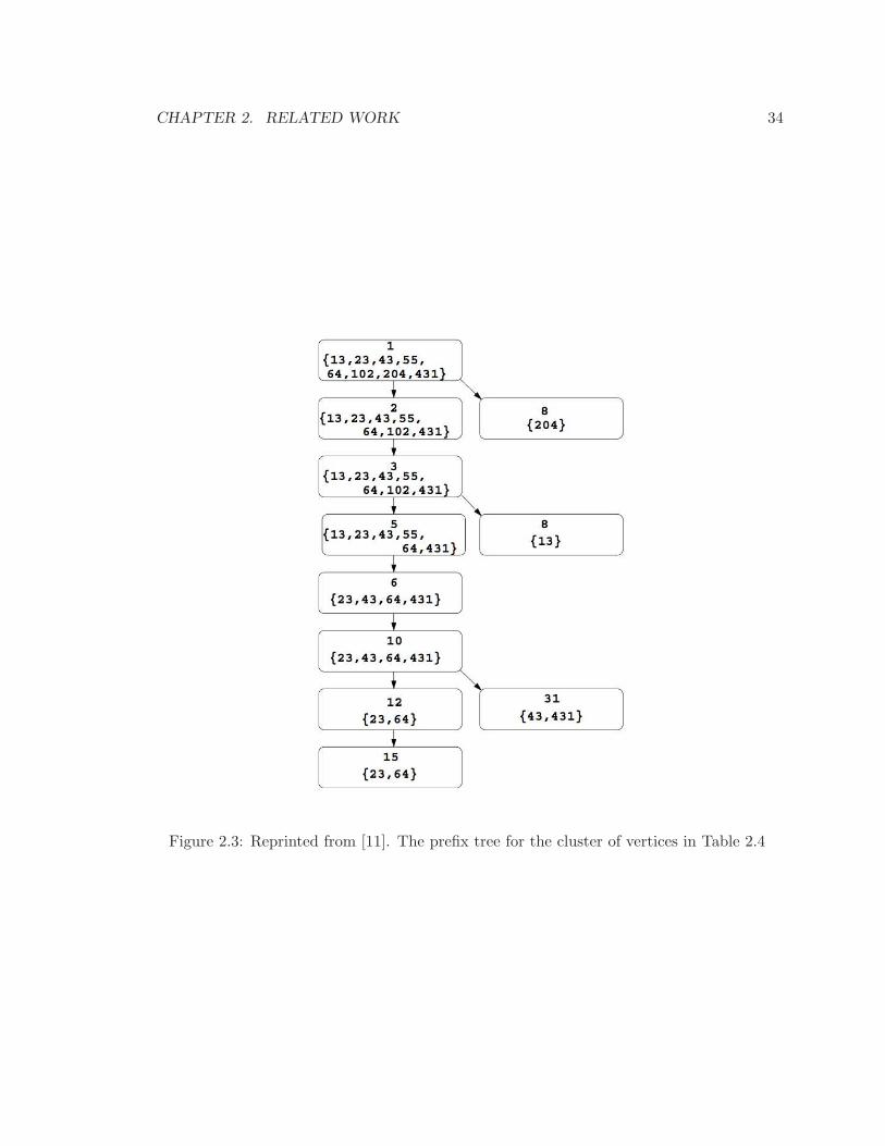
CHAPTER 2. RELATED WORK 34
Figure 2.3: Reprinted from [11]. The prefix tree for the cluster of vertices in Table 2.4

CHAPTER 2. RELATED WORK 35
The simplest rule for updating a node’s label would be the majority vote among the
neighbors of that node. However, using the majority vote as the updating rule, it has
been observed that the label propagation algorithm tends to produce a very large cluster,
containing most of the nodes. To resolve this problem a variety of methods have been
proposed [42, 2].
The following variant of the label propagation family, called Absolute Pott Model (APM) [56],
has been used by the WebGraph compression framework as a subroutine to reorder the ver-
tices of a network: let λ1, · · · , λk be those labels that have appeared on the neighborhood
of node u. Let ki (1 ≤ i ≤ k) be the number of neighbors of u having label λi. Let vi be
the number of nodes in the whole graph with label λi. According to the APM algorithm,
the label of u will be updated to λi such that it maximises the following:
ki − γ(vi − ki)
The intuition is that for adding a particular node to cluster λi, the number of non-existing
edges (vi−ki) is also important. It is not hard to see that the density of resulting communities
would be at least γ/(γ +1). Algorithm 3 presents the pseudo code for the APM algorithm.
Algorithm 3 The APM algorithm. λ is a function that will provide the cluster labels.λ−1(l) is the set of nodes having label l.
π ← a random permutation of G’s nodes;for all x: λ(x)← x, v(x)← 1;while no update is possible dofor all i = 0, 1, · · · , n− 1 dofor every label l, kl ← |λ−1(l) ∩NG(π(i))|l← argmaxl[kl − γ(v(l)− kl)]decrement v(λ(π(i)))λ(π(i))← lincrement v(λ(π(i)))
end forend while
CHAPTER 2. RELATED WORK 36
2.4.3 Structural Clustering Method
We explain a clustering method in this section which we believe potentially can be used in
both aggregation-based and order-based compression frameworks. The idea of this approach
is to view the clusters as a set of nodes that have similar neighbors. A cluster is consisted
of a “nucleus” and a “boundary”. The vertices in the nucleus does not belong to any other
cluster. However, vertices in the boundary of a cluster might belong to other clusters as
well. First, we define the similarity measure for two nodes u and v [63]:
σ(u, v) =|N(v) ∩N(u)|
√
|N(v)| × |N(u)|,
where N(u) is the set of the neighbors of u. Having this notion of similarity in mind the
ǫ-neighborhood of u is the set of those neighbors of u that their similarity to u is at least ǫ:
Nǫ(u) = {v ∈ N(u)|σ(u, v) ≥ ǫ}
The method uses two parameters, ǫ and µ. A node u is a core if the ǫ-neighborhood of it, has
at least µ vertices. Then, if we only consider the core vertices and the edges among them,
in this new network, a connected component of the core vertices is forming the nucleus of a
cluster. The boundary of a cluster is consisted of those non-core vertices that are belonging
to Nǫ(u) for at least a vertex u in the nucleus.
In [63], the formalism to capture this idea has been introduced. Moreover, an algorithm
to discover all the clusters for given ǫ and µ is developed. The algorithm works as follows:
in one scan it identifies the core vertices. If a core vertex u is not assigned to a cluster
yet, the algorithm generates a new cluster Id for it. Then, in a breadth first search style, it
grows the cluster around u. The algorithm is linear in the number of edges of the network.
Note that, the reference coding technique in the order-based approach also uses the
similarity of the neighborhood of the vertices. In this technique the out-neighbor list of one
node is encoded by referring to the out-neighbor list of another node. To have an effective
reference coding we need to find an ordering in which the nodes with similar neighbors are
close to each other. Since the structural clustering method clusters the nodes based on the
CHAPTER 2. RELATED WORK 37
similarity of their neighbors, potentially it can be exploited to generate an ordering in which
reference coding technique is effective. However, the structural clustering method assumes
the graph is undirected. An immediate challenge is to extend the idea to directed networks.
2.4.4 Spectral Clustering
Spectral clustering method uses the algebraic properties of the adjacency matrix of the
network. The solid theoretical foundations and the running time efficiency are two critical
advantages of the method. The spectral clustering method as a preprocessing step embeds
the nodes of the graph into a low-dimensional space. Likewise, the order-based approach
also as a preprocessing step embeds the nodes into a one-dimensional space (an ordering of
the nodes can be considered as an embedding of the nodes into a line). However, spectral
clustering assumes that the network is symmetric, i.e., undirected. A popular technique to
apply the spectral clustering on directed networks is to simply ignore the direction of the
edges. Here, we cover the basic concepts and algorithms of the spectral clustering. We also
provide a theoretical analysis to reveal the intuition behind the method.
Definitions and Backgrounds
For a square matrix X, a non-zero vector v is an eigenvector of X if there is a real number
λ such that:
Xv = λv
The real number λ is the eigenvalue of X corresponding to v. A square matrix X is
symmetric positive semidefinite if and only if it is symmetric and for any v ∈ Rn, we
have vTXv ≥ 0. It is a basic fact in linear algebra [15], that a n × n symmetric positive
semidefinite matrix has n distinct, pairwise orthogonal eigenvectors, and the eigenvalues
corresponding to them are non-negative.
The adjacency matrix A of an undirected graph G is a |V (G)| × |V (G)| square matrix,
where Ai,j = Aj,i = 1, if i and j are connected and Ai,j = 0 otherwise5. Let di be the degree
5To be perfectly precise, we assume that V (G) = {1, · · · , |V (G)|}
CHAPTER 2. RELATED WORK 38
of vertex i, then, the degree matrix D is a diagonal |V (G)|× |V (G)| matrix, where Di,i = di
and Di,j = 0 if i 6= j. The unnormalized Laplacian matrix of G is defined as:
L = D −A
For vector v, vi is the entry corresponding to node i. The following proposition summarizes
the basic properties of L [38]:
Proposition 1. Let n = |V (G)|. The following properties holds for unnormalized Laplacian
matrix L:
1. For every vector v ∈ Rn we have:
vTLv =1
2
n∑
i=1
n∑
j=1
Ai,j(vi − vj)2
2. L is symmetric positive semidefinite.
3. L has n non-negative real-valued eigenvalues 0 = λ1 ≤ λ2 ≤ · · · ≤ λn
Proof. Item 1
vTLv = vTDv − vTAv =n∑
i=1
div2i −
n∑
i=1
n∑
j=1
Ai,jvivj
Notice that di =∑n
j=1Ai,j . Therefore we have:
vTLv =n∑
i=1
n∑
j=1
Ai,jv2i −
n∑
i=1
n∑
j=1
Ai,jvivj
Since Ai,j = Aj,i, we have:
n∑
i=1
n∑
j=1
Ai,jv2i =
1
2
(
n∑
i=1
n∑
j=1
Ai,jv2i +
n∑
i=1
n∑
j=1
Ai,jv2j
)
Therefore,
vTLv =1
2
(
n∑
i=1
n∑
j=1
Ai,jv2i − 2
n∑
i=1
n∑
j=1
Ai,jvivj +
n∑
i=1
n∑
j=1
Ai,jv2j
)
=1
2
n∑
i=1
n∑
j=1
Ai,j(vi − vj)2
CHAPTER 2. RELATED WORK 39
Item 2
L is symmetric because both D and A are symmetric, and is positive semidefinite because
according to part (1), for v ∈ Rn, we have:
vTLv =1
2
n∑
i=1
n∑
j=1
Ai,j(vi − vj)2 ≥ 0
Item 3
L is symmetric positive semidefinite, thus, it has n non-negative eigenvalues. Observe that
for the constant one vector 1, we have L1 = 0× 1. Therefore, the smallest eigenvalue of L
is zero.
As a convention, we sort the eigenvalues of a Laplacian matrix L, in a non-decreasing
order: 0 = λ1 ≤ λ2 ≤ · · · ≤ λn. λ1 is the first eigenvalue of L, λ2 is the second and so
on. Likewise, the i-th eigenvector is the eigenvector corresponding to the i-th eigenvalue.
There are many different variants of spectral clustering methods in the literature. The
common ingredient, however, is that somehow they use the eigenvectors of the Laplacian
for a preprocessing step. For example, let v be an eigenvector of the Laplacian L , with a
non-zero eigenvalue. Then, the mapping ϕ(i) = vi is an embedding of the vertices to a line.
This is particularly interesting, because the vertices of a network can be considered as a set
of points in a high dimensional Euclidean space. So, one can think of the spectral methods
as a dimension reduction technique. We like to remind the reader that many clustering
methods, e.g. K-means, perform much better on low dimensional data.
Algorithm 4 shows a simple variant of spectral clustering algorithms.
Algorithm 4 Pseudo code for the spectral clustering
1: Let A be the adjacency matrix and D be the diagonal degree matrix2: Let L = D −A3: Let v1,v2, · · · ,vk be the first k eigenvectors of L4: Let U ∈ R
k×n be the matrix consisted of v1, · · · ,vk as columns5: Let yi ∈ R
k be the vector corresponding to the i-th row of U6: Cluster {yi|i = 1, · · · , n} using K-mean algorithm
CHAPTER 2. RELATED WORK 40
Justification
Unfortunately, there is no solid theorem that relates the eigenvalues and eigenvectors of the
Laplacian of a network to the clusters of it. However in this section, we try to justify the
relevance of the eigenvectors in an intuitive fashion. We show that the second eigenvector is
related to the relaxation of a variant of min-cut problem, which is NP-hard otherwise. The
material in this section comes from [38].
A natural formulation for node clustering is to find a partitioning such that it minimizes
the number of edges with end points in different partitions. For a subset C of vertices C is
the set of those vertices that does not belong to C. Cut(C, C) is the number of edges that
have one end in C and the other end in C. For a partition C1, · · · , Ck of vertices, we define:
Cut(C1, · · · , Ck) =1
2
k∑
i=1
Cut(Ci, Ci)
In particular for k = 2, the problem of finding a minimum Cut can be solved in polynomial
time. However, in many cases it separates a single vertex from the rest of the network. To
resolve this problem the notion of RatioCut tries to favor a sort of balanced partitioning:
RatioCut(C1, · · · , Ck) =1
2
k∑
i=1
Cut(Ci, Ci)
|Ci|
Unfortunately, finding the partitioning that minimizes the RatioCut ,even for k = 2, is
NP-hard [60]. For k = 2, we show that how the spectral clustering can be seen as solving a
relaxed version of the RatioCut minimization problem.
The objective is to find a subset C ⊂ V such that:
minC⊂V
RatioCut(C, C)
First, we rewrite the problem using the Laplacian matrix L. For a subset C ⊂ V , f =
(f1, · · · , fn)T ∈ Rn is defined as follows:
fi =
√
|C|/|C| if i ∈ C
−√
|C|/|C| if i ∈ C(2.2)
CHAPTER 2. RELATED WORK 41
Having this definition for f , we can write:
fTLf =1
2
n∑
i=1
n∑
j=1
Ai,j(fi − fj)2
=1
2
∑
i∈C
∑
j∈C
Ai,j
(
√
|C|/|C|+√
|C|/|C|)2
+1
2
∑
i∈C
∑
j∈C
Ai,j
(
−√
|C/|C| −√
|C|/|C|)2
= Cut(C, C)( |C||C| +
|C||C| + 2
)
= Cut(C, C)( |C|+ |C||C| +
|C|+ |C||C|
)
= RatioCut(C, C)× |V |
Therefore, minimizing fTLf is equivalent to minimizing the RatioCut:
minC⊂V fTLf , subject to:
fi defined as in Equation 2.2
Moreover, the multiplication of f and the constant one vector is:
f1 =n∑
i=1
fi =∑
i∈C
√
|C||C| −
∑
i∈C
√
|C||C| = |C|
√
|C||C| − |C|
√
|C||C| = 0
Also the square of norm 2 of vector f is:
‖f‖2 =n∑
i=1
f2i = |C| |C||C| − |C||C||C| = n
Hence, the addition of these two new constraints would not change the solution of the
minimization problem:
minC⊂V fTLf , subject to:
1) fi defined as in equation 2.2
2) f1 = 0
3) ‖f‖ = √n
CHAPTER 2. RELATED WORK 42
However, this is still a NP-hard problem [38]. The variables fi can take two particular
values, according to equation 2.2. The immediate relaxation of this optimization problem is
to relax variables fi to take any real value. This leads to the following optimization problem:
minf∈Rn fTLf , subject to:
1) f1 = 0
2) ‖f‖ = √nThis problem can be solved in polynomial time. In fact, by the Rayleigh-Ritz theorem
(e.g. see Section 5.5.2 of [39]) it can be shown that the eigenvector corresponding to the
second smallest eigenvalue is the solution for this optimization problem. So, in some sense
the second eigenvector of L is an estimation for minimizing the RatioCut. However, this
solution is not a partitioning yet. In order to get the partitioning we need another step. A
simple heuristic to obtain the partitions would be:
vi ∈ C if fi ≥ 0
vi ∈ C if fi < 0
This simple heuristic is not working for k > 2. Instead, we can consider fi as points in R
and use a more general clustering algorithm like K-means to partition the points. This is
exactly the spectral clustering method we presented in Algorithm 4. Notice that the first
eigenvector, that is used in Algorithm 4, is the constant one vector, therefore, it does not
have any influence in the output of K-means algorithm. Also we like to note that, using a
similar argument one can show that the following standard trace minimization problem is
a relaxation of RatioCut problem for general k:
minH∈Rk×n Tr(HTLH), subject to:
HTH = I,
where, Tr(X) for a square matrix X is the sum of the entries on the diagonal of X. The
same Rayleigh-Ritz theorem [39] tells us that the solution of this optimization problem is
the matrix H consisted of the first k eigenvectors of L as columns.
CHAPTER 2. RELATED WORK 43
2.5 The Graph Layout Problem
In the classical graph theory, the problem of finding a “good” ordering of the nodes with
respect to minimizing/maximizing a given objective function has a long history. The appli-
cations of this family of problem include VLSI circuit design, numerical analysis and more.
These problems fall in the class of combinatorial optimization problems. Often for nontrivial
objective functions, finding the ordering that has the optimal cost is NP-hard [29, 47]. In
this section, we refer to these family of problems as graph layout problems.
Both graph layout problem and order-based compression approach are looking for a
“good” ordering of the nodes. The notion of goodness in a layout problem is captured
by an objective function, while in the order-based compression framework the goodness of
an ordering is measured by the compression rate. A promising direction to pursue is to
introduce an objective function for a layout such that it captures the requirements of the
compression framework.
We review the results and heuristic algorithms for a few classical variants of the graph
layout problems. Even though, typically the objective function in these classical variants
are not explicitly connected to the compression framework, we believe studying them would
help us to understand the nature and challenges of these family of problems.
2.5.1 Definitions and Theoretical Results
In this section, first we present a few formal definitions, and illustrate them using a toy
example. Also, we give a short review of the theoretical algorithmic results. The material
of this section mostly comes from the Dıaz et al. survey [19]. A layout ϕ of an undirected
graph G = (V,E) is a bijective function ϕ : V → {1, · · · , n}, where n is the number of
vertices of the graph. Given a graph G, a layout ϕ of G, and an integer i, we define the set
of left vertices of i:
L(i, ϕ,G) = {u ∈ V : ϕ(u) ≤ i},
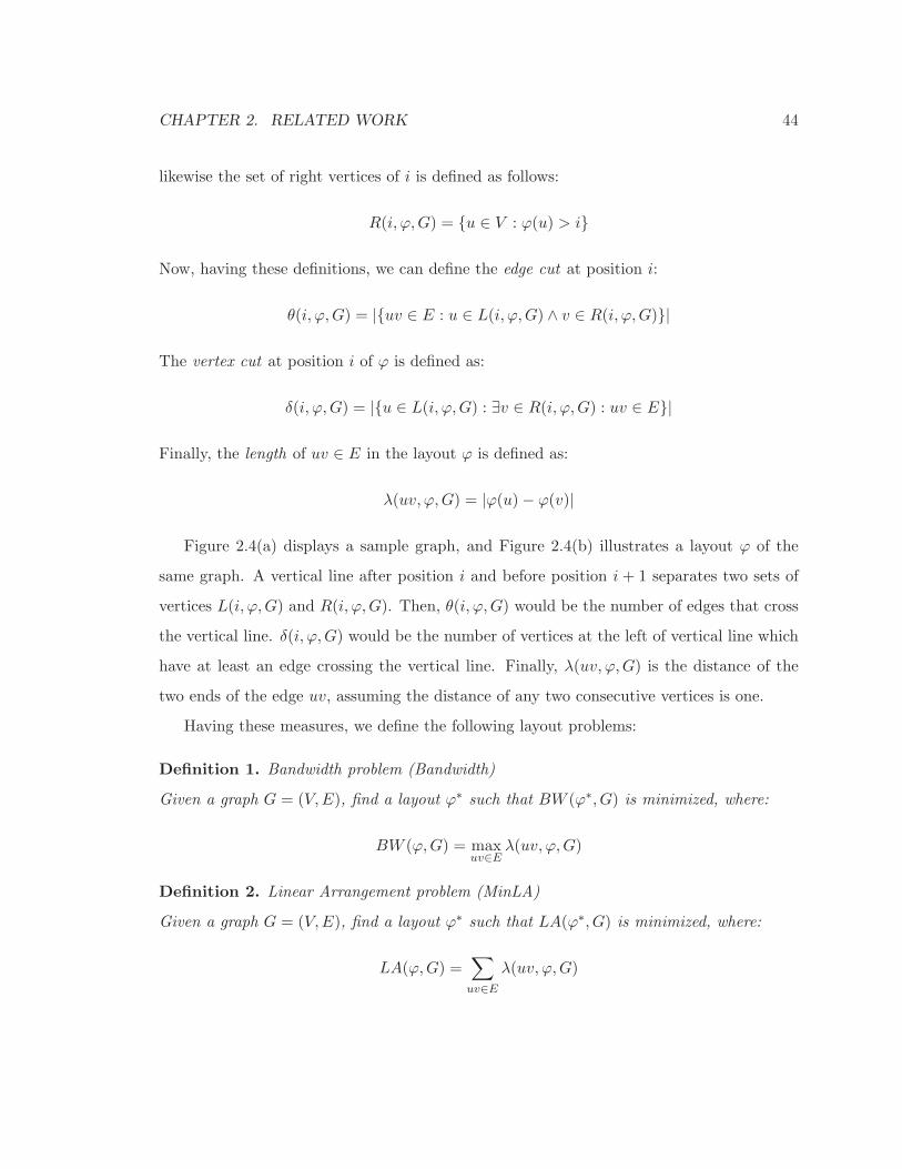
CHAPTER 2. RELATED WORK 44
likewise the set of right vertices of i is defined as follows:
R(i, ϕ,G) = {u ∈ V : ϕ(u) > i}
Now, having these definitions, we can define the edge cut at position i:
θ(i, ϕ,G) = |{uv ∈ E : u ∈ L(i, ϕ,G) ∧ v ∈ R(i, ϕ,G)}|
The vertex cut at position i of ϕ is defined as:
δ(i, ϕ,G) = |{u ∈ L(i, ϕ,G) : ∃v ∈ R(i, ϕ,G) : uv ∈ E}|
Finally, the length of uv ∈ E in the layout ϕ is defined as:
λ(uv, ϕ,G) = |ϕ(u)− ϕ(v)|
Figure 2.4(a) displays a sample graph, and Figure 2.4(b) illustrates a layout ϕ of the
same graph. A vertical line after position i and before position i + 1 separates two sets of
vertices L(i, ϕ,G) and R(i, ϕ,G). Then, θ(i, ϕ,G) would be the number of edges that cross
the vertical line. δ(i, ϕ,G) would be the number of vertices at the left of vertical line which
have at least an edge crossing the vertical line. Finally, λ(uv, ϕ,G) is the distance of the
two ends of the edge uv, assuming the distance of any two consecutive vertices is one.
Having these measures, we define the following layout problems:
Definition 1. Bandwidth problem (Bandwidth)
Given a graph G = (V,E), find a layout ϕ∗ such that BW (ϕ∗, G) is minimized, where:
BW (ϕ,G) = maxuv∈E
λ(uv, ϕ,G)
Definition 2. Linear Arrangement problem (MinLA)
Given a graph G = (V,E), find a layout ϕ∗ such that LA(ϕ∗, G) is minimized, where:
LA(ϕ,G) =∑
uv∈E
λ(uv, ϕ,G)
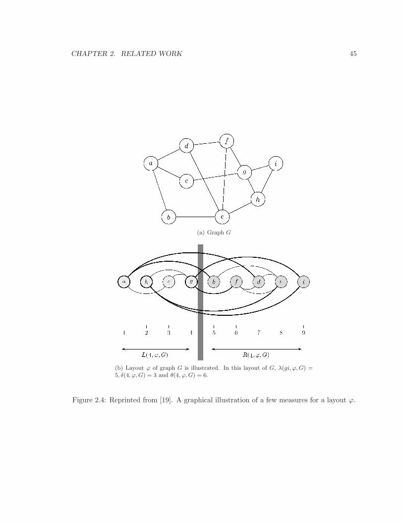
CHAPTER 2. RELATED WORK 45
(a) Graph G
(b) Layout ϕ of graph G is illustrated. In this layout of G, λ(gi, ϕ,G) =5, δ(4, ϕ,G) = 3 and θ(4, ϕ,G) = 6.
Figure 2.4: Reprinted from [19]. A graphical illustration of a few measures for a layout ϕ.
CHAPTER 2. RELATED WORK 46
Definition 3. Cut Width problem (Cutwidth)
Given a graph G = (V,E), find a layout ϕ∗ such that CW (ϕ∗, G) is minimized, where:
CW (ϕ,G) = max1≤i≤|V |
θ(i, ϕ,G)
Definition 4. Vertex Separation problem (VertSep)
Given a graph G = (V,E), find a layout ϕ∗ such that V S(ϕ∗, G) is minimized, where:
V S(ϕ,G) = max1≤i≤|V |
δ(i, ϕ,G)
All of these problems have been proven to be NP-hard for general undirected graphs [19].
Except MinLA, the other three are NP-hard even when the input is restricted to graphs
with maximum degree 3. Surprisingly, Bandwidth problem is NP-hard, when the input is
restricted to trees with maximum degree 3.
An α-approximation algorithm guarantees that the output is at most α times worse
than the optimal solution [1, 25], where α is the approximation factor. To the best of
our knowledge, the Bandwidth problem has a O(log3 n√log log n)-approximation algorithm.
The best approximation factor known for MinLA is O(√log n log log n). There are O(log2 n)-
approximation algorithms for both VertSep and CutWidth [24, 19].
Even thought, these approximation algorithms are interesting from a theoretical point of
view, they are not practical. The major tool for establishing these upper bounds is a gener-
alized linear programming technique, known as the Ellipsoid method. A linear program is an
optimization problem in which the goal is to maximize/minimize a linear objective function,
subject to a set of linear inequality constraints. The power of the Ellipsoid method is that,
under some conditions, the running time does not depend on the number of constraints.
Therefore, if the linear program has polynomial number of variables and exponential num-
ber of constraints, the Ellipsoid method could solve the problem in polynomial time. In
practice, the method suffers from a very poor running time. This motivates us to discuss
the heuristic algorithms.

CHAPTER 2. RELATED WORK 47
2.5.2 Heuristics
In this subsection we briefly discuss the heuristics for the layout problems. However, we
should mention that the layout problems are not initially motivated by the social network
analysis applications. As a result, there are not much experimental results on the perfor-
mance of these heuristics on social networks. The techniques and ideas that we describe
here are general and can be used for any layout problem.
We discuss three different approaches, spectral sequencing, a multi-scale framework and
local search technique. The first technique is merely based on the second eigenvector of the
laplacian of the network, while the multi-scale framework is using a coarsening approach,
to recursively reduce the size of the network.
Spectral Sequencing: The algorithm starts by computing the second eigenvector v2 of
Laplacian matrix L (see section 2.4.4). Then, the layout ϕ is defined as follows:
ϕ(x) < ϕ(y) ⇐⇒ v2(x) < v2(y),
where x and y are two nodes of the graph, and v2(x) is the entry of vector v2 corresponding
to node x. The ties would be broken arbitrarily. This is a very simple, yet effective heuristic.
As it is mentioned in [49], this ordering is particularly effective for those networks that have
a sort of geometric structure, e.g. VLSI networks.
Local Search: The local search technique starts with an initial layout ϕ and improves the
layout by applying local changes. The critical design factor in a local search scheme is the
definition of local changes. The following two operations are introduced in [49]:
1. F lip2: randomly chooses two vertices and switch their position in the layout ϕ.
2. F lip3: randomly chooses three vertices and rotates their positions in the layout ϕ.
The reason for choosing these operations is efficiency of applying the operation and com-
puting the cost for the new layout. This method is somehow the complement of spectral
sequencing. The performance of this local search scheme on the network with geometric
CHAPTER 2. RELATED WORK 48
structure is worse than spectral sequencing, However, it outperforms the spectral sequenc-
ing method for the random networks.
A natural idea to overcome the weakness of the local search is to use the spectral se-
quencing method as the initialization phase [48]. This combination is quit effective and
improves the result both for geometric and random graph. To the best of our knowledge,
there is no reported results for the performance of these methods on the social networks.
Multi-Scale Framework: Figure 2.5 illustrates the basic ideas of multi-scale framework.
The algorithm consisted of three phases: coarsening, initialization and uncoarsening. In
the coarsening phase, recursively, a few nodes aggregate in a super-node, and the relations
between these super-nodes are captured by weighted edges. The coarsening phase stops
when the size of the graph is small enough, e.g. ten super-nodes. Then, for the coarsest
aggregated network, using an exhaustive search, the best ordering is computed. In the
uncoarsening phase, using the layout from each level, the algorithm initiate the layout for
the next finer level. Then, a local search technique is deployed to improve the finer layout.
The framework has been used successfully for solving different problems [33, 57, 13]. One
can think of this framework as a recursive local search scheme. Arguably, coarsening phase
is the most critical step of the framework. Here, we explain the coarsening phase in [57]
that is based on an algebraic multi-grid (AMG) technique [58].
In the AMG technique, a matrix P projects the fine graph to the coarse graph. Let Af
be the adjacency matrix of the fine graph. The projection is as follows:
Ac ← P TAfP,
where Ac is the adjacency matrix of the coarse graph. Projection matrix P is a real-valued
n × m matrix, in which n and m are the number of nodes in the fine and coarse graph,
respectively. Notice that using the AMG projection, the coarse graph will be a weighted
graph, even if the fine graph is unweighted. In the rest of this section, we explain how to
construct the projection matrix P , and the meaning behind this algebraic projection.
Let Gf be the fine network. We start by choosing a set of seed nodes S ⊂ V (Gf ). One
CHAPTER 2. RELATED WORK 49
can think of these seed nodes as the center of the future super-nodes of the coarse graph.
We have to choose subset S so that for node i /∈ S:∑
j∈S
Afi,j
/
∑
j∈V (Gf )
Afi,j ≥ θ, (2.3)
where, θ is a threshold parameter. Intuitively, this means that any node of the fine graph
should be “well represented” by its neighbors in S. The set S can be constructed in one
scan. If a node i is not “well represented” by S, i.e., does not satisfy the inequality 2.3, we
greedily add it to S. Let I : S → {1, · · · , |S|} be a bijective function from seed nodes S to
integers {1, · · · , |S|}. The n× |S| projection matrix P is defined as follows:
Pi,I(j) =
Afij/
∑
k∈NSiAf
ik if i ∈ V (Gf )\S ∧ j ∈ NSi
1 if i ∈ S ∧ j = i
0 otherwise
Where, NSi is the neighbors of i in S. One can think of Pi,I(j) as the likelihood of i
belonging to super-node I(j). The merit of this approach is that a node i proportionally
could aggregate to several super-nodes. This leads to a more accurate coarsening process.
In the coarse graph Gc, the weight of the edge that connecting two super-nodes p and q
is:
Acp,q =
∑
k
∑
l 6=k
Pk,pAfk,lPl,q
This means that the contribution of every edge (k, l) in Gf to the edge (p, q) in Gc is
proportional to the likelihood of k and l belonging to super-nodes p and q, respectively.
2.6 Summary
We discussed two completely different approaches towards compressing social networks. The
first approach uses the idea of aggregating a set of nodes with a similar set of neighbors
to a super-node, while the second approach exploits an ordering of the nodes in which the
similar nodes tend to be close to each other.
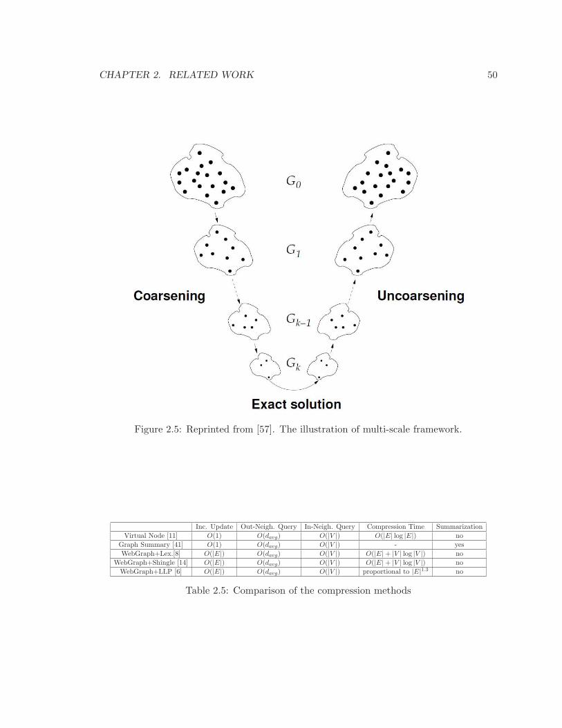
CHAPTER 2. RELATED WORK 50
Figure 2.5: Reprinted from [57]. The illustration of multi-scale framework.
Inc. Update Out-Neigh. Query In-Neigh. Query Compression Time Summarization
Virtual Node [11] O(1) O(davg) O(|V |) O(|E| log |E|) no
Graph Summary [41] O(1) O(davg) O(|V |) - yes
WebGraph+Lex.[8] O(|E|) O(davg) O(|V |) O(|E|+ |V | log |V |) no
WebGraph+Shingle [14] O(|E|) O(davg) O(|V |) O(|E|+ |V | log |V |) no
WebGraph+LLP [6] O(|E|) O(davg) O(|V |) proportional to |E|1.3 no
Table 2.5: Comparison of the compression methods
CHAPTER 2. RELATED WORK 51
We reviewed a few methods for the dense subgraph mining and clustering of social
networks. A semi-complete bipartite subgraph mining technique and a clustering algorithm
known as Absolute Pott Model had been explained. The semi-complete bipartite subgraph
mining is a basic component of the Virtual Node compression scheme, and the Absolute Pott
Model is used in the LLP algorithm. A structural clustering algorithm that partitions the
nodes based on the similarity of their neighbors has been discussed. We remind that both
the reference encoding technique in the order-based approach and the aggregation technique
exploit the similarity of neighbors of a group of nodes to achieve compression. The spectral
clustering is discussed for three different reasons: (1) it has solid theoretical foundation, (2)
the method is scalable, and most importantly, (3) the spectral clustering is based on an
embedding of the nodes to a low dimension space. Note that, the order-based compression
methods also use an embedding of the nodes to a one-dimensional space.
Finally, we reviewed a family of combinatorial graph problems, known as graph layout
problems. The goal is to find an ordering of the nodes that minimizes a given objective
function. Different variants of these problems have been introduced and the hardness and
approximation results along with a few major heuristic algorithms have been reviewed. This
line of research can be inspiring if one tries to capture the notion of a “good” ordering for
the order-based approach by introducing a combinatorial objective function.
Table 2.5 summarizes and compares different features of the compression algorithms.
Generally speaking, the aggregation-based methods have the advantage of allowing efficient
incremental updates and providing a summarization of the communities (dense subgraphs)
of the network. On the other hand, the order based methods are more efficient regarding the
compression time. They both can answer the out-neighbor query efficiently, however, the
order-based methods have larger over-head due to bit-level operations. To answer the in-
neighbor query efficiently, both approaches has to replicate the data by storing the transpose
of the data.
Comparing the compression rate of the aggregation-based methods and order-based
methods, is not trivial for two reasons: first, the two approaches use different measures
CHAPTER 2. RELATED WORK 52
as the compression rate. Second, they use different datasets to report the experimental
results. We can resolve the first issue by assuming that to store an identifier of a node, one
uses 32 bits in the aggregation-base approach. With this assumption, a compression rate of
0.15, i.e., the number of edges in compressed graph over the number of edges in the original
graph, is corresponding to 0.15× 32 = 3.36 bits/edge. Using this criteria, roughly one can
imply that the compression rate of the order-based approach is better comparing to the
aggregation-based approach. Among the order-based methods, WebGraph+LLP, i.e., the
WebGraph framework coupled with the LLP ordering, has the best compression rate.
We believe both aggregation and order-based approaches suffer from major disadvantages
that disqualify them as a general purpose storage scheme for social networks. The order-
based methods does not allow incremental updates, while the aggregation methods are only
effective if the social network is rich with a certain type of very dense subgraphs (depending
on the aggregation technique). Both approaches do not allow efficient in-neighbor query
answering without replicating the data.
2.7 How this thesis is related and different from the existing
work
In Chapter 3, we will introduce GPSN compression framework, a novel compression frame-
work that can be regarded as a generalization of the order-based approach. This framework
allows efficient in-neighbor and out-neighbor queries, and incremental updates. We provide
an upper-bound on the compression rate for a simple setting of our framework. Similar
to order-based methods the framework exploits a “lineup” of nodes. However, the order-
based approach uses an ordering of nodes in which each node appear exactly once. As
oppose to the GPSN framework in which, the “lineup” is a sequence of nodes, with possible
replications. We refer to this sequence as a “linearization” of nodes.
On the other hand, similar to the aggregation-based approach, existing of dense sub-
graphs is essential to the effectiveness of the GPSN compression framework. The framework
tries to position the nodes that are part of a dense subgraph, in the proximate positions
CHAPTER 2. RELATED WORK 53
of the sequence. Chapter 4 discusses a lossless compression method designed based on
the principles of the GPSN framework. We compare the compression rate of our lossless
compression scheme with WebGraph+Shingle [14].
The lossy compression scheme is presented in Chapter 5. Motivated by graph layout
problems, we turn the problem of finding a good “linearization” of nodes to an optimization
problem. Although, our objective function is more complicated comparing to those that
we have discussed in Section 2.5. We believe this complexity is due to the combinatorial
nature of the network compression problem, and is unavoidable. The heuristic to optimize
such an objective function is designed according to the complex combinatorial nature of the
objective function, and is among the contributions of this dissertation.
Chapter 3
GPSN Compression Framework
In this chapter, we discuss our approach towards having a General Purpose Social Network
(GPSN) compression framework. A GPSN compression framework allows network analysis
algorithms directly operate on the compressed version of a network. This is particularly
interesting because most of the algorithms implicitly assume that the network fits in the
main memory. However, in the age of the online social media, applications have to analyze
and manipulate networks with hundreds of millions of nodes and billions of edges.
For the rest of this section, we take a formal approach to provide a theoretical analysis
of our framework. We introduce the notion of k-cover and k-linearization, and using these
notions, provide an upper bound on the compression rate of a simple setting of our frame-
work. The theoretical analysis provided in this section is interesting and could serve as an
evidence of the effectiveness of our framework. However, in practice often a more realistic
setting is desirable. We leave the discussion on the practical aspects of the framework for
the next two chapters.
3.1 The GPSN Compression Framework
Note that, in Section 1.1, we already discussed the core idea of the GPSN compression
framework in an intuitive fashion. We start the section by introducing two definitions that
54
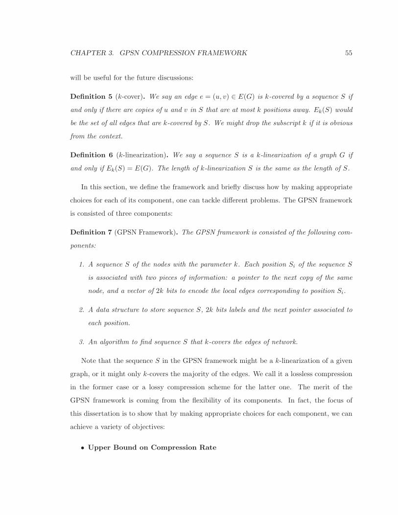
CHAPTER 3. GPSN COMPRESSION FRAMEWORK 55
will be useful for the future discussions:
Definition 5 (k-cover). We say an edge e = (u, v) ∈ E(G) is k-covered by a sequence S if
and only if there are copies of u and v in S that are at most k positions away. Ek(S) would
be the set of all edges that are k-covered by S. We might drop the subscript k if it is obvious
from the context.
Definition 6 (k-linearization). We say a sequence S is a k-linearization of a graph G if
and only if Ek(S) = E(G). The length of k-linearization S is the same as the length of S.
In this section, we define the framework and briefly discuss how by making appropriate
choices for each of its component, one can tackle different problems. The GPSN framework
is consisted of three components:
Definition 7 (GPSN Framework). The GPSN framework is consisted of the following com-
ponents:
1. A sequence S of the nodes with the parameter k. Each position Si of the sequence S
is associated with two pieces of information: a pointer to the next copy of the same
node, and a vector of 2k bits to encode the local edges corresponding to position Si.
2. A data structure to store sequence S, 2k bits labels and the next pointer associated to
each position.
3. An algorithm to find sequence S that k-covers the edges of network.
Note that the sequence S in the GPSN framework might be a k-linearization of a given
graph, or it might only k-covers the majority of the edges. We call it a lossless compression
in the former case or a lossy compression scheme for the latter one. The merit of the
GPSN framework is coming from the flexibility of its components. In fact, the focus of
this dissertation is to show that by making appropriate choices for each component, we can
achieve a variety of objectives:
• Upper Bound on Compression Rate

CHAPTER 3. GPSN COMPRESSION FRAMEWORK 56
The first natural question regarding our method is on the possibility of proving an
upper bound on the compression rate. We know that for a k-linearization of length
l, the GPSN framework uses l × (2k + log2(l)) bits. Hence, to have an upper bound
on the compression rate, it is sufficient to prove an upper bound on the length of the
k-linearization. Having such an upper bound for arbitrary value of k is not easy to
obtain. However, we can have such an analysis for the special case of k = 1. For the
rest of this chapter we prove an upper bound for the compression rate of our framework
when it is restricted to the simple setting of k = 1. For this special case, we use a
simple array data structure to represent the input network. From an algorithmic point
of view, we show that to find the shortest sequence S that 1-covers all the edges of a
graph G, one has to cover the edges of G by the least number of paths, such that any
edge appears exactly once in the exactly one path. This can be seen as a generalization
of the Eulerian path problem where the objective is to cover the edges of the graph
by exactly one path.
• Lossless Compression
As the second major part of the thesis, we focus on evaluating our framework on real
world social networks, as a lossless compression scheme. The setting is as follows: we
fix the parameter k, and design a greedy heuristic to find a sequence S that k-linearize
a given graph G. We use an array data structure to store the sequence S and a binary
tree to store the meta-data (see Chapter 4). The focus of the experimental study is
to evaluate the compression rate for different values of k. We also report the query
processing time of our lossless compression scheme.
• Lossy Compression
In Chapter 5, we change the settings of our problem substantially. Instead of looking
for a sequence S that is a k-linearization of a given graph G, we fix k and l, and ask for
a sequence S of length l that k-covers those “important” edges of G. For the purpose
of our work, an edge is “important” if it contributes to the global community structure
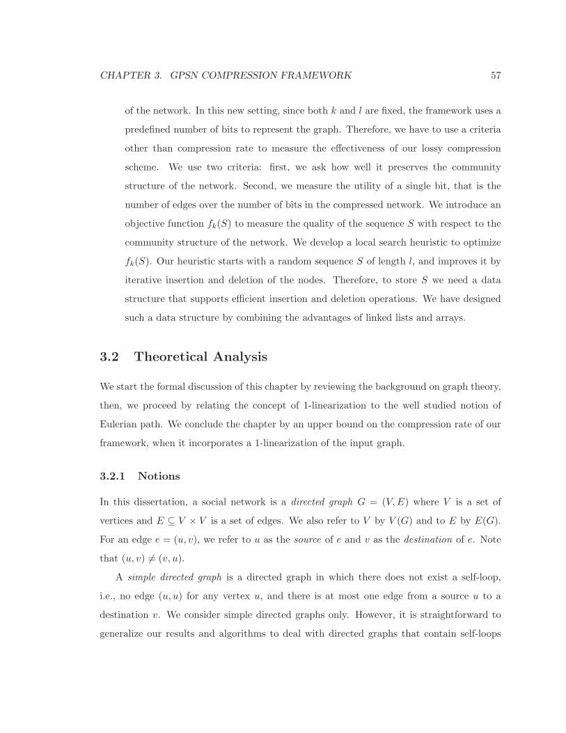
CHAPTER 3. GPSN COMPRESSION FRAMEWORK 57
of the network. In this new setting, since both k and l are fixed, the framework uses a
predefined number of bits to represent the graph. Therefore, we have to use a criteria
other than compression rate to measure the effectiveness of our lossy compression
scheme. We use two criteria: first, we ask how well it preserves the community
structure of the network. Second, we measure the utility of a single bit, that is the
number of edges over the number of bits in the compressed network. We introduce an
objective function fk(S) to measure the quality of the sequence S with respect to the
community structure of the network. We develop a local search heuristic to optimize
fk(S). Our heuristic starts with a random sequence S of length l, and improves it by
iterative insertion and deletion of the nodes. Therefore, to store S we need a data
structure that supports efficient insertion and deletion operations. We have designed
such a data structure by combining the advantages of linked lists and arrays.
3.2 Theoretical Analysis
We start the formal discussion of this chapter by reviewing the background on graph theory,
then, we proceed by relating the concept of 1-linearization to the well studied notion of
Eulerian path. We conclude the chapter by an upper bound on the compression rate of our
framework, when it incorporates a 1-linearization of the input graph.
3.2.1 Notions
In this dissertation, a social network is a directed graph G = (V,E) where V is a set of
vertices and E ⊆ V × V is a set of edges. We also refer to V by V (G) and to E by E(G).
For an edge e = (u, v), we refer to u as the source of e and v as the destination of e. Note
that (u, v) 6= (v, u).
A simple directed graph is a directed graph in which there does not exist a self-loop,
i.e., no edge (u, u) for any vertex u, and there is at most one edge from a source u to a
destination v. We consider simple directed graphs only. However, it is straightforward to
generalize our results and algorithms to deal with directed graphs that contain self-loops
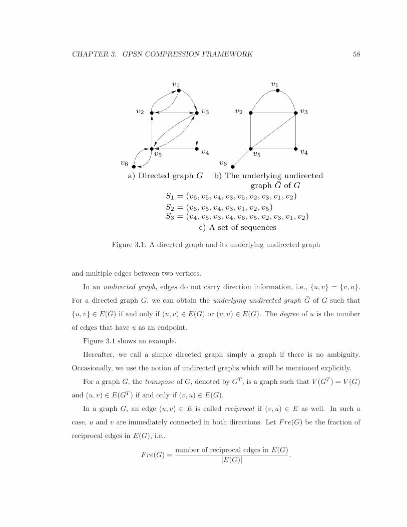
CHAPTER 3. GPSN COMPRESSION FRAMEWORK 58
�� ��
��
��
��
��
�� ��
��
��
��
��
v1
v2 v3
v4v5v6
S2 = (v6, v5, v4, v3, v1, v2, v5)
S1 = (v6, v5, v4, v3, v5, v2, v3, v1, v2)
S3 = (v4, v5, v3, v4, v6, v5, v2, v3, v1, v2)
v1
v2 v3
v4v5v6
graph G of Gb) The underlying undirecteda) Directed graph G
c) A set of sequences
Figure 3.1: A directed graph and its underlying undirected graph
and multiple edges between two vertices.
In an undirected graph, edges do not carry direction information, i.e., {u, v} = {v, u}.For a directed graph G, we can obtain the underlying undirected graph G of G such that
{u, v} ∈ E(G) if and only if (u, v) ∈ E(G) or (v, u) ∈ E(G). The degree of u is the number
of edges that have u as an endpoint.
Figure 3.1 shows an example.
Hereafter, we call a simple directed graph simply a graph if there is no ambiguity.
Occasionally, we use the notion of undirected graphs which will be mentioned explicitly.
For a graph G, the transpose of G, denoted by GT , is a graph such that V (GT ) = V (G)
and (u, v) ∈ E(GT ) if and only if (v, u) ∈ E(G).
In a graph G, an edge (u, v) ∈ E is called reciprocal if (v, u) ∈ E as well. In such a
case, u and v are immediately connected in both directions. Let Fre(G) be the fraction of
reciprocal edges in E(G), i.e.,
Fre(G) =number of reciprocal edges in E(G)
|E(G)| .

CHAPTER 3. GPSN COMPRESSION FRAMEWORK 59
Therefore, G = GT if and only if Fre(G) = 1.
3.2.2 Neighbor Queries in Directed Graphs
In a directed graph G, there are two types of neighbors. For a vertex u ∈ V (G), v1 ∈ V (G)
is an out-neighbor of u if (u, v1) ∈ E(G). Moreover, v2 ∈ V (G) is an in-neighbor of u if
(v2, u) ∈ E(G). An out-neighbor query on u intents to find the set of out-neighbors of u.
Similarly, an in-neighbor query on u would search for all in-neighbors of u.
Example 3 (Neighbor queries). In Figure 3.1(a), an out-neighbor query on v5 in G returns
{v2, v3, v6}. An in-neighbor query on v5 returns {v3, v4, v6}. Please note that v3 and v6 are
both out-neighbors and in-neighbors of v5, since there are reciprocal edges between v3 and v5
as well as between v5 and v6.
All the existing methods for compressing web graphs or social networks encode only
outgoing edges. Consequently, those methods can only answer out-neighbor queries directly.
3.2.3 Eulerian Paths
A path P of length k in a graph G is a sequence of edges (u1, u2), (u2, u3), . . . , (uk, uk+1),
where (ui, ui+1) ∈ E(G) (1 ≤ i ≤ k). For the purpose of simplicity, we often write path P
as (u1, u2, . . . , uk+1). P is a simple path if u1, . . . , uk+1 are unique among one another.
Definition 8 (Eulerian path). An Eulerian path for an undirected graph is a path in the
graph which visits each edge of the graph exactly once.
Example 4 (Eulerian path). In Figure 3.1(b), path S1 is an Eulerian path for G, S2 is not
because it does not visit edge {v5, v3}. Likewise, S3 is not an Eulerian path, because it is
not a path – {v4, v6} is not an edge in the graph G.
It is well known that a connected undirected graph G has an Eulerian path if and only
if it has at most two vertices with odd degree.
A simple algorithm to construct the Eulerian path which dates back to 1883, known as
Fleury’s algorithm, is as follows: we start with a vertex of odd degree. If there is no such a
CHAPTER 3. GPSN COMPRESSION FRAMEWORK 60
vertex, we start with any vertex. At each step we move across an edge whose deletion does
not disconnect the graph, unless there is no other choice. We repeat this process until no
edge is left.
3.2.4 1-Linearization
Here, we establish the connection between the notions of 1-linearization and Eulerian path
for a given graph G. The following proposition is immediate:
Proposition 2 (Lower bound of 1-linearization). Given a directed graph G, the lower bound
for the length of the 1-linearization of G is
|E(G)|+ 1 = (1− Fre(G)
2)|E(G)|+ 1,
moreover the bound is tight if and only if G has an Eulerian path, or equivalently it has at
most two vertices of odd degrees.
Example 5 (Lower bound of 1-linearization). The lower bound for the length of 1-linearization
of G in Figure 3.1 is 9, since |E(G)| = 8. We can write |E(G)| in terms of |E(G)| usingFre(G). Since Fre(G) = 6/11, |E(G)| = (1− 6/11
2 )|E(G)| = 8.
Unlike the Eulerian path construction problem which is an existence problem, finding
the optimal 1-linearization is an optimization problem. No matter what structure a graph
has, always there exists an optimal (shortest) 1-linearization for the graph. The following
lemma gives the length of an optimal 1-linearization of an arbitrary directed graph.
Lemma 1. The minimum length for an 1-linearization of an arbitrary directed graph G is
|E(G)|+max{nodd/2, 1}, where nodd is the number of vertices with odd degrees in G.
Proof. In any undirected graph G, the sum of degrees of all vertices is even. Thus, the
number of vertices with odd degrees is also even.
We first prove by induction that for any graph G we can obtain an 1-linearization of
length |E(G)|+max{nodd/2, 1}.Basis: For nodd = 0 and nodd = 2, the claim follows from proposition 2.
CHAPTER 3. GPSN COMPRESSION FRAMEWORK 61
Induction: Since nodd must be even, we assume that the lemma holds for nodd = 2k
(k ≥ 1), and consider the case when nodd = 2(k + 1). There are two subcases.
In the first subcase, there are two vertices u and v with odd degrees such that they are
not connected in G. We add an edge {u, v} to G and call the new graph G∗. Since G∗ has
only 2k vertices with odd degrees, applying the induction assumption, we can obtain an
1-linearization of G∗ with length |E(G∗)| + k = |E(G)| + k + 1. Since E(G) ⊂ E(G∗) the
1-linearization of G∗ is also an 1-linearization for G.
In the second subcase, all vertices with odd degrees are connected. We arbitrarily take
two vertices u and v with odd degrees and remove the edge {u, v} from G. Let us call the
resulting graph G∗. Again, G∗ has 2k vertices with odd degrees. Therefore, there is an
1-linearization with length |E(G∗)| + k = |E(G)| − 1 + k for G∗. Since the 1-linearization
for G∗ does not cover {u, v}, we have to add u and v to the end of the sequence. Therefore
we just build an 1-linearization for G of length |E(G)|+ k + 1, as desired.
We prove that |E(G)|+max{nodd/2, 1} is also a lower bound for the 1-linearizations for
G. For nodd = 0 and nodd = 2, simply applying Proposition 2 gives the bound.
Now, let us consider the case where nodd ≥ 4. Let v(i) be the vertex that appears in the
position i of an 1-linearization L. For a vertex u with an odd degree in G which appears
in neither the first nor the last position of L, we denote by Pu = {i|v(i) = u} the set of all
appearances of u in L. There are in total at least nodd − 2 such vertices.
For any interior position i in L, there are two edge slots in L: (i − 1, i) and (i, i + 1).
Consider all the edge slots associated with the positions in Pu. At least one of these slots
must be a “waste”, that is, there is no edge appearing in the slot or the edge in the slot also
appears in some other slot. Otherwise, the degree of u is 2|Pu|, which is an even number.
In the best scenario, two vertices with odd degrees can share a wasted edge slot. There-
fore, we have at least (nodd− 2)/2 wasted edge slots. In addition, we need |E(G)| edge slotsto cover the edges of G. Therefore, in total L has to have at least |E(G)|+ nodd/2− 1 edge
slots. Hence, the length of L cannot be smaller than |E(G)|+max{nodd/2, 1}.
Please note that the induction in the proof of Lemma 1 also gives an linear algorithm

CHAPTER 3. GPSN COMPRESSION FRAMEWORK 62
Algorithm 5 to find an optimal 1-linearization of G
Input: Graph GOutput: L1: Let O be the set of all vertices in G with odd degree2: EE = ∅; RE = ∅3: // eliminate all the nodes with odd degree by adding or removing edges between pair
of them4: while there are u, v ∈ O do5: if (u, v) /∈ E(G) then6: add (u, v) to E(G)7: add (u, v) to EE8: else9: remove (u, v) from E(G)
10: add (u, v) to RE11: end if12: remove u and v from O13: end while14: Let L be the Eulerian tour of G given by Hierholzer’s algorithm15: for all (u, v) ∈ RE do16: add u and v to the end of L17: end for
to find an optimal 1-linearization of a graph G. Before presenting the algoirthm we explain
Hierholzer’s algorithm [32] that is a linear time (linear to the number of edges) algorithm for
finding an Eulerian path in a given graph. The algorithm is as follows: choose any vertex v
as the starting vertex, and follow a trail of edges from that vertex until returning to v. Note
that if the degree of all edges are even it is not possible to stuck in any vertex other than v,
because by entering any vertex other than v, the number of remaining edges for that vertex
will be an odd number and therefore nonzero. Thus, we will endup at v. However, the tour
might not cover all the edges. In case there is a node in the current tour that has unused
edges, start another trail, using only unused edges, from that vertex, and join the new tour
to the old one. By the use of the simple doubly linked list data structre to maintain the list
of all nodes with unused edges and the list of unused edges for each node, this algorithm
can be implemented in linear time.
Algorithm 5 returns an optimal 1-linearization L of a given graph G. The proof of
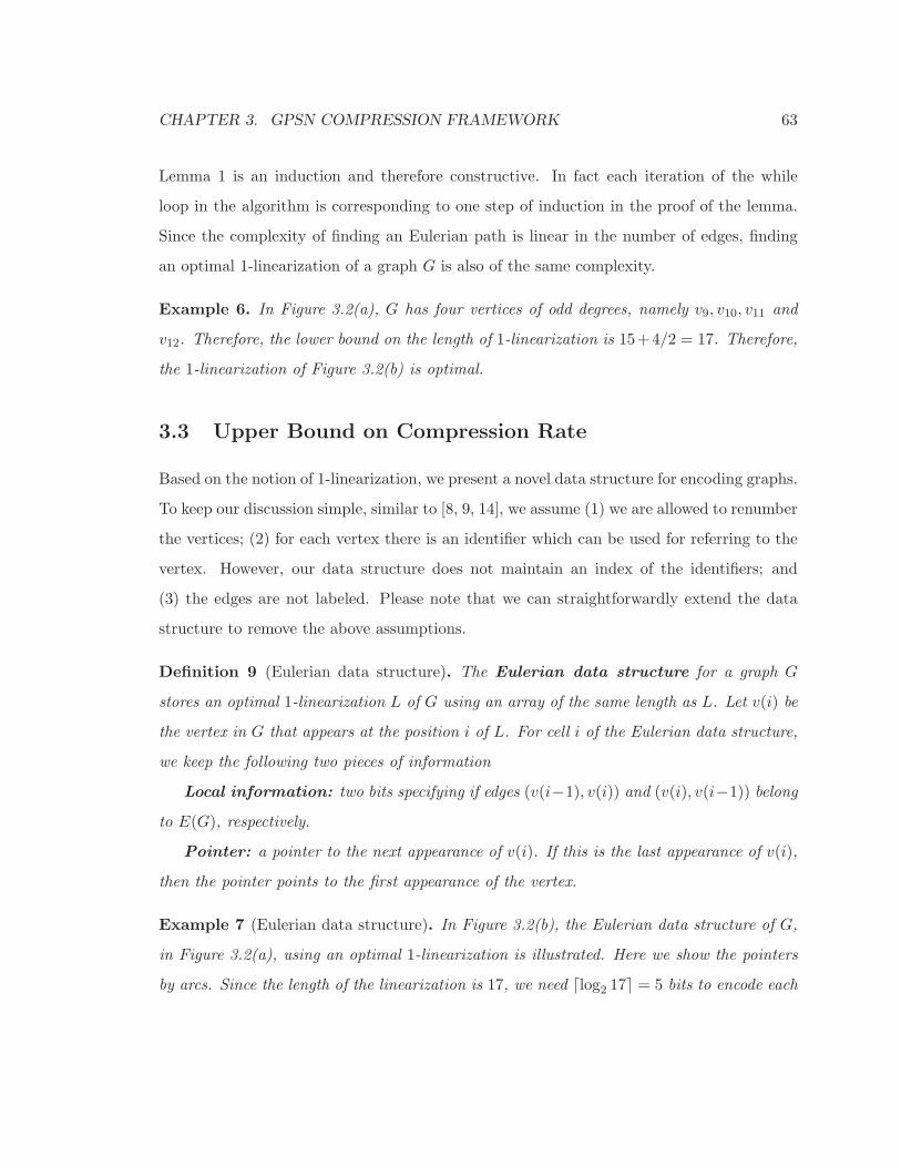
CHAPTER 3. GPSN COMPRESSION FRAMEWORK 63
Lemma 1 is an induction and therefore constructive. In fact each iteration of the while
loop in the algorithm is corresponding to one step of induction in the proof of the lemma.
Since the complexity of finding an Eulerian path is linear in the number of edges, finding
an optimal 1-linearization of a graph G is also of the same complexity.
Example 6. In Figure 3.2(a), G has four vertices of odd degrees, namely v9, v10, v11 and
v12. Therefore, the lower bound on the length of 1-linearization is 15+4/2 = 17. Therefore,
the 1-linearization of Figure 3.2(b) is optimal.
3.3 Upper Bound on Compression Rate
Based on the notion of 1-linearization, we present a novel data structure for encoding graphs.
To keep our discussion simple, similar to [8, 9, 14], we assume (1) we are allowed to renumber
the vertices; (2) for each vertex there is an identifier which can be used for referring to the
vertex. However, our data structure does not maintain an index of the identifiers; and
(3) the edges are not labeled. Please note that we can straightforwardly extend the data
structure to remove the above assumptions.
Definition 9 (Eulerian data structure). The Eulerian data structure for a graph G
stores an optimal 1-linearization L of G using an array of the same length as L. Let v(i) be
the vertex in G that appears at the position i of L. For cell i of the Eulerian data structure,
we keep the following two pieces of information
Local information: two bits specifying if edges (v(i−1), v(i)) and (v(i), v(i−1)) belongto E(G), respectively.
Pointer: a pointer to the next appearance of v(i). If this is the last appearance of v(i),
then the pointer points to the first appearance of the vertex.
Example 7 (Eulerian data structure). In Figure 3.2(b), the Eulerian data structure of G,
in Figure 3.2(a), using an optimal 1-linearization is illustrated. Here we show the pointers
by arcs. Since the length of the linearization is 17, we need ⌈log2 17⌉ = 5 bits to encode each
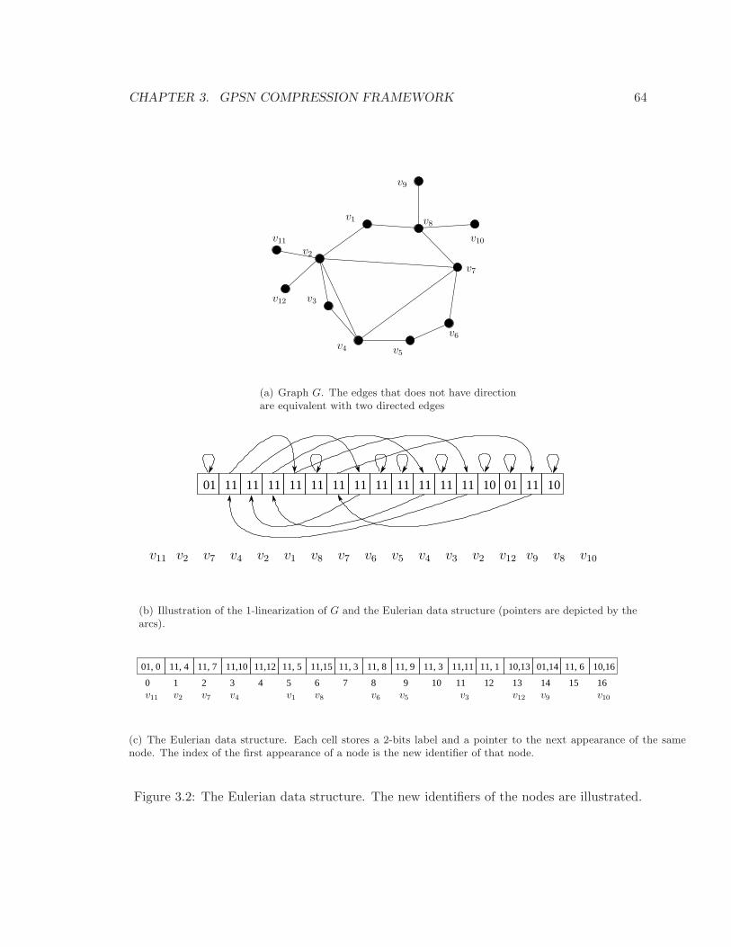
CHAPTER 3. GPSN COMPRESSION FRAMEWORK 64
v3
v5
v6
v7
v8v1
v2
v4
v9
v10v11
v12
(a) Graph G. The edges that does not have directionare equivalent with two directed edges
01 11 1011 11 11 11 11 11 11 11 11 11 101101 11
v9 v8 v10v2 v2 v2v7 v4 v1 v8 v7 v6 v5 v4 v3 v12v11
(b) Illustration of the 1-linearization of G and the Eulerian data structure (pointers are depicted by thearcs).
6 7 8 9 10 11 120 1 2 3 4 5
01, 0 11, 7 11,10 11,12 11, 5 11, 3 11, 8 11, 9 11, 3
13 14
01,14
15 16
10,1611, 611,15 11,11 11, 1 10,1311, 4
v2 v7 v4 v1 v8 v6 v5 v3 v12v11 v9 v10
(c) The Eulerian data structure. Each cell stores a 2-bits label and a pointer to the next appearance of the samenode. The index of the first appearance of a node is the new identifier of that node.
Figure 3.2: The Eulerian data structure. The new identifiers of the nodes are illustrated.
CHAPTER 3. GPSN COMPRESSION FRAMEWORK 65
pointer. Therefore, for each position we need 5+ 2 bits. In total we need 17× (5+ 2) = 119
bits.
We prove an upper bound on the size of the Eulerian data structure:
Lemma 2. An Eulerian data structure to encode a graph G uses at most
|V (G)|(
d+ 1)
2
(
1 + log(|V (G)|) + log(d+ 1))
bits, where d is the average degree of G.
Proof. Let L be an optimal 1-linearization of G (therefore for G as well). Since there are
at most |V | vertices of odd degrees in G, the upper bound for the length of L is |E(G)| +|V (G)|/2. Using 2 bits to store the local information and ⌈log2(|E(G)|+ |V (G)|/2)⌉ bits forthe pointer for each cell, in total the Eulerian data structure uses at most
(
|E(G)|+ |V (G)|/2)(
2 + ⌈log2(|E(G)|+ |V (G)|/2)⌉)
bits. We can write |E(G)| = |V (G)|d/2, where d is the average degree of G. Therefore:
|V (G)|(
d+ 1)
2
(
1 + log(|V (G)|) + log(d+ 1))
We have the following result on the compression efficiency of the Eulerian data structure.
Theorem 1. An Eulerian data structure to encode a graph G uses at most
(1− Fre(G)
2+
1
d)(
⌈log2(|V (G)|) + log2(d+ 1)⌉+ 1)
bits per edge on average, where d is the average degree of G. Moreover, using this data
structure, it is possible to answer the in-neighbor and out-neighbor queries for any vertex v
in O(∑
u∈Nvdeg(u) log |V (G)|) time, where deg(u) is the degree of vertex u in G and Nv is
the set of out-neighbors/in-neighbors of v in out-neighbor/in-neighbor queries.
CHAPTER 3. GPSN COMPRESSION FRAMEWORK 66
Proof. To get the bits/edge rate, we divide the upper bound on the size of the data structure
by the number of edges of G. We have
( |E(G)|+ |V (G)|/2|E(G)|
)(
2 + ⌈log2(|E(G)|+ |V (G)|/2)⌉)
.
Notice that we can write the ratio of |E(G)|/|E(G)| in terms of Fre(G) and also
|V (G)|2|E(G)| ≤
|V (G)|2|E(G)|
which is precisely the inverse of the average degree of G. Therefore, the bits/edge rate is at
most:(
1− Fre(G)
2+
1
d
)(
2 + ⌈log2(|E(G)|+ |V (G)|/2)⌉)
We use |E(G)| = |V (G)|d2 to further simplify the inside of the logarithm, and obtain
(
1− Fre(G)2 + 1
d
)(
2 + ⌈log2(|V (G)|d/2 + |V (G)|/2)⌉)
=(
1− Fre(G)2 + 1
d
)(
2 + ⌈log2(|V (G)|) + log2(d+ 1)− log2(2)⌉)
The upper bound is proved.
For analysis of the query processing time, we assume that the data structure is a sequence
of bits. Hence reading a pointer takes O(log(|V (G)|)) time.
Since each vertex u of G appears in at least one position in the Eulerian data structure,
we use the index of the first position of u in L as the identifier for the vertex. Therefore, for
an out-neighbor/in-neighbor query on vertex u, we have to return the positions of the first
appearances of all out-neighbors/in-neighbors of u. Fetching the local information (only two
bits) for one position takes constant time. Reading the pointer takes O(log |V (G)|) time (the
number of bits for each pointer). Since the number of copies for a vertex u is ⌈deg(u)/2⌉ inthe optimal 1-linearization of G, traversing over the linked list takes O(deg(u) log2 |V (G)|)time. By traversing the linked list corresponding to vertex u we can retrieve the positions of
all neighbors of u. However, for a neighbor v of u, the retrieved position may not be the first
appearance of v. Therefore, for each retrieved neighbor v, we have to traverse the linked list
for v to get the first appearance. So, answering an out-neighbor/in-neighbor query takes
O(log(|V (G)|)∑u∈Nvdeg(u)) time in total.
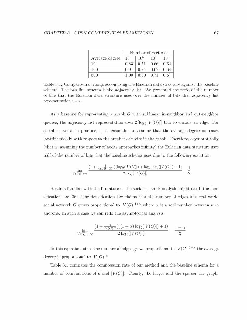
CHAPTER 3. GPSN COMPRESSION FRAMEWORK 67
Number of verticesAverage degree 103 105 107 109
10 0.83 0.71 0.66 0.64
100 0.91 0.74 0.67 0.64
500 1.00 0.80 0.71 0.67
Table 3.1: Comparison of compression using the Eulerian data structure against the baselineschema. The baseline schema is the adjacency list. We presented the ratio of the numberof bits that the Eulerian data structure uses over the number of bits that adjacency listrepresentation uses.
As a baseline for representing a graph G with sublinear in-neighbor and out-neighbor
queries, the adjacency list representation uses 2⌈log2 |V (G)|⌉ bits to encode an edge. For
social networks in practice, it is reasonable to assume that the average degree increases
logarithmically with respect to the number of nodes in the graph. Therefore, asymptotically
(that is, assuming the number of nodes approaches infinity) the Eulerian data structure uses
half of the number of bits that the baseline schema uses due to the following equation:
lim|V (G)|→∞
(1 + 1log
2|V (G)| )(log2(|V (G)|) + log2 log2(|V (G)|) + 1)
2 log2(|V (G)|) =1
2
Readers familiar with the literature of the social network analysis might recall the den-
sification law [36]. The densification law claims that the number of edges in a real world
social network G grows proportional to |V (G)|1+α where α is a real number between zero
and one. In such a case we can redo the asymptotical analysis:
lim|V (G)|→∞
(1 + 1|V (G)|α )((1 + α) log2(|V (G)|) + 1)
2 log2(|V (G)|) =1 + α
2
In this equation, since the number of edges grows proportional to |V (G)|1+α the average
degree is proportional to |V (G)|α.Table 3.1 compares the compression rate of our method and the baseline schema for a
number of combinations of d and |V (G)|. Clearly, the larger and the sparser the graph,

CHAPTER 3. GPSN COMPRESSION FRAMEWORK 68
the less bits the Eulerian data structure uses. Real life social networks are often large and
sparse, therefore, the Eulerian data structure is capable of compressing social networks.
To the best of our knowledge, the Eulerian data structure is the first schema that allows
answering both out-neighbor and in-neighbor queries in sublinear time, and provides a
nontrivial upper bound on the number of bits per edge. Note that to prove the upper
bound given by Theorem 1 we did not use any assumption on the type of the network,
therefore the result is not limited to the social networks and is valid for arbitrary graphs.
3.4 Summary
In this chapter, we introduce a compression framework. Theoretically, we prove an upper
bound on the compression rate for a simple setting of the framework. This theoretical
analysis can serve as a good evidence for the storage efficiency of our framework. For the
next two chapters of this dissertation, we are going to consider two more practical settings
for our framework.
In Chapter 4, we use the principles of the GPSN framework to design a lossless com-
pression scheme for social networks. The lossless compression scheme uses a relaxed version
of k-linearization, which we call multi level linearization. We introduce this new notion to
be adaptive to the ”skewed“ structure of the real world social network.
Chapter 4
Lossless Compression
The GPSN framework has three components, namely: (1) a linearization S of the given
graph, (2) a data structure to store the sequence S, and (3) an algorithm to build the
sequence S. In the previous chapter, we used the notion of k-linearization to prove an
upper bound for the compression rate of the GPSN framework. However, in a more realistic
setting having a fixed parameter k for linearizing a real world social network is not always
practical. For the rest of this chapter, first, we introduce a relaxed notion for linearizing a
social network. Then, we explain the data structure to store the linearization. We present a
simple greedy heuristic to build such a linearization. Finally, we conclude the chapter with
the experimental results.
4.1 Multi Level Linearization
We start our discussion based on the known fact that the edges in real world social networks
are highly correlated. The building blocks of social networks are communities. The edges
are often local in the sense that if a node belongs to a community, a statistically significant
fraction of its neighbors tend to be in the same community. Therefore, a large fraction of
the edges in a given social network are intra-community edges. Intuitively, the parameter k
in the k-linearization is trying to capture the degree of locality in the network, that is the
69
CHAPTER 4. LOSSLESS COMPRESSION 70
size of the communities in a given social network.
The size and structure of such communities have been the focus of many recent works.
While Leskovec et al. [37] suggested that the communities are typically no larger than a
hundred nodes, it is unrealistic to assume all of them have the same size. Therefore, using
multiple values of k to linearize a social network is a more effective approach. The notion
of multi-level linearization is designed to capture such intuition. A multi-level linearization
is a sequence S of nodes, such that S is partitioned to several segments and each segment
uses its own value of k. The definition of multi-level linearization is as follows:
Definition 10 (Multi-Level Linearization). A multi-level linearization of a given graph G
is a sequence S and a list of integer pairs (i1, k1), · · · , (im, km), such that i1 = 0 < i2 <
· · · , < im < length(S) and k1 > k2, · · · , km > 0. Then, assuming St = S[it, it+1 − 1] we
have1:
∪mt=1Ekt(St) = E(G),
where Ekt(St) is the set of all edges that are k-covered by St. We refer to this list as the
neighborhood scheme of S.
A commonly used notion for measuring the locality in social networks is the average
clustering coefficient [62], that is:
Acc(G) = Acc(G) =1
|V (G)|∑
v∈V (G)
2|Ev||Nv|(|Nv| − 1)
,
where Ev is the set of edges that have both ends among the neighbours of v. In social
networks, the number of vertices with a small degree is much more than the number of
vertices with a large degree. Consequently, average clustering coefficient has a bias towards
the vertices with small degrees. That is, since the low degree vertices, e.g. vertices with
degree one, tend to have large clustering coefficient, the average clustering coefficient is
misleadingly large. Therefore, to measure the locality of a network we use Global Clustering
1The notation S[it, it+1−1] refers to the subsequence of S that starts from position it and ends at position
it+1 − 1
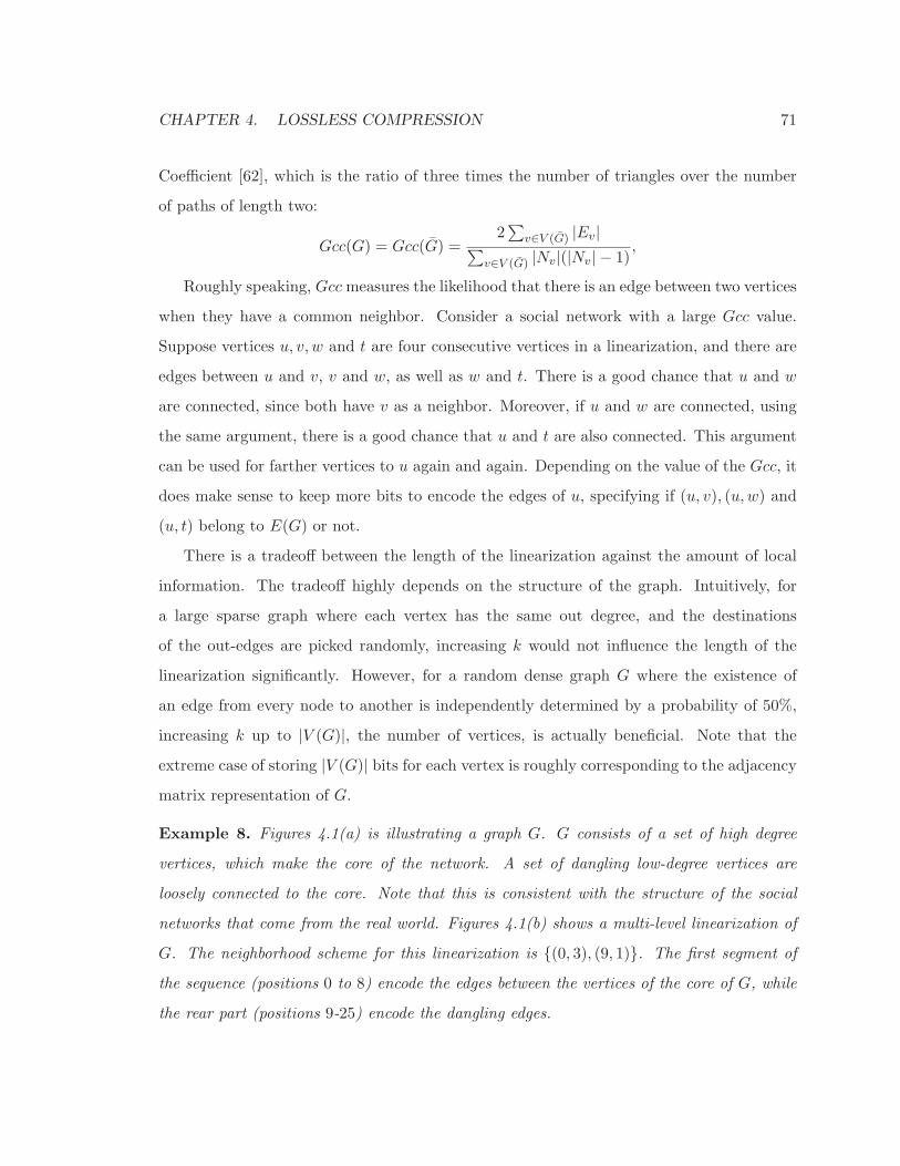
CHAPTER 4. LOSSLESS COMPRESSION 71
Coefficient [62], which is the ratio of three times the number of triangles over the number
of paths of length two:
Gcc(G) = Gcc(G) =2∑
v∈V (G) |Ev|∑
v∈V (G) |Nv|(|Nv| − 1),
Roughly speaking, Gccmeasures the likelihood that there is an edge between two vertices
when they have a common neighbor. Consider a social network with a large Gcc value.
Suppose vertices u, v, w and t are four consecutive vertices in a linearization, and there are
edges between u and v, v and w, as well as w and t. There is a good chance that u and w
are connected, since both have v as a neighbor. Moreover, if u and w are connected, using
the same argument, there is a good chance that u and t are also connected. This argument
can be used for farther vertices to u again and again. Depending on the value of the Gcc, it
does make sense to keep more bits to encode the edges of u, specifying if (u, v), (u,w) and
(u, t) belong to E(G) or not.
There is a tradeoff between the length of the linearization against the amount of local
information. The tradeoff highly depends on the structure of the graph. Intuitively, for
a large sparse graph where each vertex has the same out degree, and the destinations
of the out-edges are picked randomly, increasing k would not influence the length of the
linearization significantly. However, for a random dense graph G where the existence of
an edge from every node to another is independently determined by a probability of 50%,
increasing k up to |V (G)|, the number of vertices, is actually beneficial. Note that the
extreme case of storing |V (G)| bits for each vertex is roughly corresponding to the adjacency
matrix representation of G.
Example 8. Figures 4.1(a) is illustrating a graph G. G consists of a set of high degree
vertices, which make the core of the network. A set of dangling low-degree vertices are
loosely connected to the core. Note that this is consistent with the structure of the social
networks that come from the real world. Figures 4.1(b) shows a multi-level linearization of
G. The neighborhood scheme for this linearization is {(0, 3), (9, 1)}. The first segment of
the sequence (positions 0 to 8) encode the edges between the vertices of the core of G, while
the rear part (positions 9-25) encode the dangling edges.
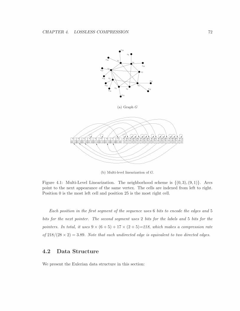
CHAPTER 4. LOSSLESS COMPRESSION 72
v3
v5
v6
v7
v8
v2
v4
v9
v10
v1
v11
v12
v13
v14
v15
v16
v17
v18
v19
(a) Graph G
000 111001 101011 101101 101101 101101 101101 110101 100011 000
v9
01
v10
10
v8
11 01 10
v13v4
1001 11
v14v3 v15
1001 11
v16v2 v17
1001 11
v18v1 v19v1v2 v3 v4 v5 v6 v7 v8 v2
01 1011
v11v6 v12
(b) Multi-level linearization of G.
Figure 4.1: Multi-Level Linearization. The neighborhood scheme is {(0, 3), (9, 1)}. Arcspoint to the next appearance of the same vertex. The cells are indexed from left to right.Position 0 is the most left cell and position 25 is the most right cell.
Each position in the first segment of the sequence uses 6 bits to encode the edges and 5
bits for the next pointer. The second segment uses 2 bits for the labels and 5 bits for the
pointers. In total, it uses 9× (6 + 5) + 17× (2 + 5)=218, which makes a compression rate
of 218/(28× 2) = 3.89. Note that each undirected edge is equivalent to two directed edges.
4.2 Data Structure
We present the Eulerian data structure in this section:
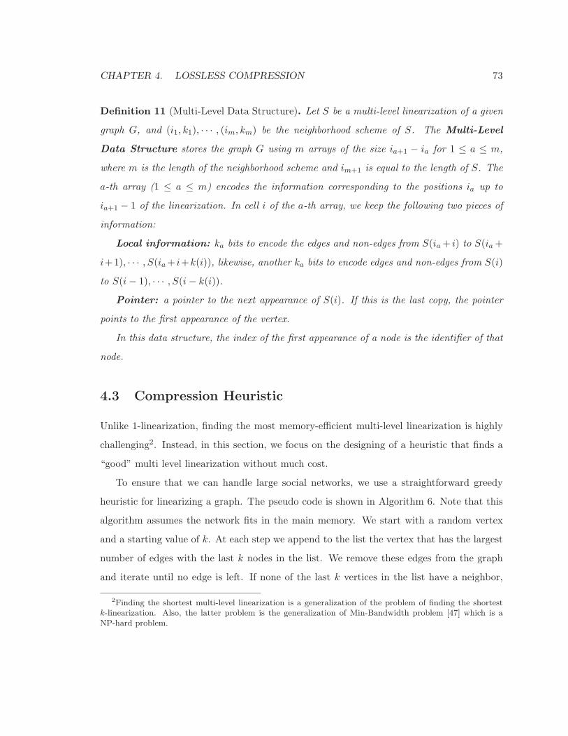
CHAPTER 4. LOSSLESS COMPRESSION 73
Definition 11 (Multi-Level Data Structure). Let S be a multi-level linearization of a given
graph G, and (i1, k1), · · · , (im, km) be the neighborhood scheme of S. The Multi-Level
Data Structure stores the graph G using m arrays of the size ia+1 − ia for 1 ≤ a ≤ m,
where m is the length of the neighborhood scheme and im+1 is equal to the length of S. The
a-th array (1 ≤ a ≤ m) encodes the information corresponding to the positions ia up to
ia+1 − 1 of the linearization. In cell i of the a-th array, we keep the following two pieces of
information:
Local information: ka bits to encode the edges and non-edges from S(ia+ i) to S(ia+
i+1), · · · , S(ia+ i+k(i)), likewise, another ka bits to encode edges and non-edges from S(i)
to S(i− 1), · · · , S(i− k(i)).Pointer: a pointer to the next appearance of S(i). If this is the last copy, the pointer
points to the first appearance of the vertex.
In this data structure, the index of the first appearance of a node is the identifier of that
node.
4.3 Compression Heuristic
Unlike 1-linearization, finding the most memory-efficient multi-level linearization is highly
challenging2. Instead, in this section, we focus on the designing of a heuristic that finds a
“good” multi level linearization without much cost.
To ensure that we can handle large social networks, we use a straightforward greedy
heuristic for linearizing a graph. The pseudo code is shown in Algorithm 6. Note that this
algorithm assumes the network fits in the main memory. We start with a random vertex
and a starting value of k. At each step we append to the list the vertex that has the largest
number of edges with the last k nodes in the list. We remove these edges from the graph
and iterate until no edge is left. If none of the last k vertices in the list have a neighbor,
2Finding the shortest multi-level linearization is a generalization of the problem of finding the shortestk-linearization. Also, the latter problem is the generalization of Min-Bandwidth problem [47] which is aNP-hard problem.

CHAPTER 4. LOSSLESS COMPRESSION 74
Algorithm 6 to find a multi level linearization of G
Input: K, reducing factor RF (0 ≤ RF ≤ 1), density threshold DT (0 ≤ DT ≤ 1) andGraph G
Output: Linearization L of G1: initialize L to an empty list2: while |E(G)| ≥ 1 do3: let u be a random node with nonzero degree4: append u to L5: {let X be the set of the last K vertices in L}6: while X has at least one neighbor in V (G)−X do7: let v be the node which has the most number of edges to and from X8: remove all edges between v and vertices in X9: edgecount+ = degold(v)− degnew(v)
10: append v to L11: if Length(L)%1000==0 then12: if edgecount/(2 ∗K ∗ 1000) < DT then13: K = K ∗RF14: end if15: edgecount = 016: end if17: end while18: end while
then we pick a random node with non-zero degree and continue from there.
As we are removing the edges of the graph, the graph becomes sparser and sparser and
eventually the rear part of the linearization may have very few new edges to encode. To
be adaptive, we watch the average local density for the recent positions in the list (the last
1000 positions3 as shown in Algorithm 6). Once it drops below a certain density threshold
DT , we reduce k by multiplying it to a predefined reducing factor RF . Note that, this
algorithm guarantees that the length of the neighborhood scheme is short, i.e. O(log k),
assuming 0 < RF < 1.
We chose to use a simple heuristic to examine the feasibility of using the GPSN frame-
work for compressing social networks. Our method leaves space for further improvement
which could be the subject for future work.
3Experimentally we used the last 100 up to 10000 positions for computing the average local density. Itturns out that the algorithm is not sensitive to this number as long as it is more than a few hundreds.
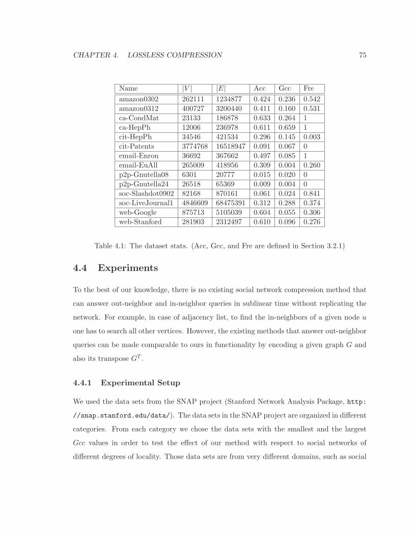
CHAPTER 4. LOSSLESS COMPRESSION 75
Name |V | |E| Acc Gcc Fre
amazon0302 262111 1234877 0.424 0.236 0.542
amazon0312 400727 3200440 0.411 0.160 0.531
ca-CondMat 23133 186878 0.633 0.264 1
ca-HepPh 12006 236978 0.611 0.659 1
cit-HepPh 34546 421534 0.296 0.145 0.003
cit-Patents 3774768 16518947 0.091 0.067 0
email-Enron 36692 367662 0.497 0.085 1
email-EuAll 265009 418956 0.309 0.004 0.260
p2p-Gnutella08 6301 20777 0.015 0.020 0
p2p-Gnutella24 26518 65369 0.009 0.004 0
soc-Slashdot0902 82168 870161 0.061 0.024 0.841
soc-LiveJournal1 4846609 68475391 0.312 0.288 0.374
web-Google 875713 5105039 0.604 0.055 0.306
web-Stanford 281903 2312497 0.610 0.096 0.276
Table 4.1: The dataset stats. (Acc, Gcc, and Fre are defined in Section 3.2.1)
4.4 Experiments
To the best of our knowledge, there is no existing social network compression method that
can answer out-neighbor and in-neighbor queries in sublinear time without replicating the
network. For example, in case of adjacency list, to find the in-neighbors of a given node u
one has to search all other vertices. However, the existing methods that answer out-neighbor
queries can be made comparable to ours in functionality by encoding a given graph G and
also its transpose GT .
4.4.1 Experimental Setup
We used the data sets from the SNAP project (Stanford Network Analysis Package, http:
//snap.stanford.edu/data/). The data sets in the SNAP project are organized in different
categories. From each category we chose the data sets with the smallest and the largest
Gcc values in order to test the effect of our method with respect to social networks of
different degrees of locality. Those data sets are from very different domains, such as social

CHAPTER 4. LOSSLESS COMPRESSION 76
networks, web graphs, peer-to-peer networks, collaborative networks, citation networks,
and co-purchasing networks. Table 4.1 provides the statistics of these networks and a short
descriptions. The description of the datasets according to http://snap.stanford.edu/
data:
• amazon0302: this network is collected by crawling Amazon website. It is based on
“Customers Who Bought This Item Also Bought” feature of the website. If a product
x is frequently co-purchased with product y, the graph contains a directed edge from
x to y. The network was collected in March 02 2003.
• ca-CondMat: the Arxiv COND-MAT (Condense Matter Physics) is a collaboration
network from the e-print arXiv and covers scientific collaborations among authors of
papers submitted to Condense Matter category. If an author x co-authored a paper
with author y, the graph contains an undirected edge from x to y. If the paper is
co-authored by k authors this generates a completely connected subgraph on k nodes.
The data cover papers in the period of January 1993 to April 2003. This period starts
within a few months of the inception of the arXiv, and thus represents essentially the
complete history of its COND-MAT section.
• ca-HepPh: Arxiv HEP-PH (High Energy Physics - Phenomenology) is a collaboration
network from the e-print arXiv, and covers scientific collaborations among authors,
based on papers submitted to the High Energy Physics Phenomenology category. If
an author x co-authored a paper with author y, the graph contains an undirected
edge from x to y. If the paper is co-authored by k authors this generates a completely
connected (sub)graph on k nodes.
The data cover papers in the period of January 1993 to April 2003. This period starts
within a few months of the inception of the arXiv, and thus represents essentially the
complete history of the HEP-PH section.
• cit-HepPh: the Arxiv HEP-PH (High Energy Physics Phenomenology) is a citation
graph from the e-print arXiv, and covers all the citations within a dataset of 34,546

CHAPTER 4. LOSSLESS COMPRESSION 77
papers with 421,578 edges. If a paper x cites paper y, the graph contains a directed
edge from x to y. If a paper cites a paper outside the dataset, the graph does not
represent any information about this.
The data cover papers in the period from January 1993 to April 2003. This period
starts within a few months of the inception of the arXiv, and therefore represents
essentially the complete history of the HEP-PH section.
• cit-Patents: the U.S. patent dataset is maintained by the National Bureau of Eco-
nomic Research. The data set cover 37 years (January 1, 1963 to December 30, 1999),
and include all the utility patents granted during this period, including 3,923,922
patents. The citation graph includes all citations made by patents granted between
1975 and 1999, including 16,522,438 citations. For the patents dataset there are
1,803,511 nodes for which there is no information about their citations (only in-links
are available).
• email-Enron: the Enron email communication data cover all the email communication
within a dataset of about half million emails. This data was originally made public,
and posted to the web, during a federal investigation. Nodes of the network are email
addresses and if an address x sent at least one email to address y, the network contains
an undirected edge from x to y. Note that for non-Enron email addresses, we only
observe their communication with the Enron email addresses.
• email-EuAll: this network is generated using email data from a large European re-
search institution. For a period from October 2003 to May 2005, we have anonymous
information about all incoming and outgoing emails of the research institution. For
each email message, we know the time, the sender and the recipient of that email. In
total, we have 3,038,531 emails, sent or received by 287,755 different email addresses.
• p2p-Gnutella08: a snapshot of the Gnutella peer-to-peer file sharing network from Au-
gust 2002. The nodes of the network represent hosts, and edges represent connections
between the Gnutella hosts.
CHAPTER 4. LOSSLESS COMPRESSION 78
• p2p-Gnutella24: another snapshot of the Gnutella peer-to-peer file sharing network
from August 2002. The nodes of the network represent hosts, and edges represent
connections between the Gnutella hosts.
• soc-Slashdot0902 slashdot.org is a technology-related news website which is known for
its specific user community. The website features user-submitted and editor-evaluated
technology oriented news. In 2002, the website introduced the Slashdot Zoo fea-
ture which allows users to tag each other as friends or foes. The network represents
friend/foe links among the users of Slashdot. The network is collected in February
2009.
• soc-LiveJournal1: LiveJournal is a free on-line social network with almost 10 million
members; a significant fraction of these members are highly active. For example,
roughly 300,000 users update their content in any given 24-hour period. LiveJournal
allows members to maintain journals, individual and group blogs, and it allows people
to declare which other members are their friends. The data was released on 2006
• web-Google: this network is the web-graph of google.com domain. The nodes of the
network represent web pages in the domain, and directed edges represent hyper-links
among them. The data set released in summer 2002 as part of Google Programming
Contest.
• web-Stanford: this network is the web-graph of stanford.edu domain. The nodes of the
network represent web pages in the domain, and directed edges represent hyper-links
among them. The data was collected in 2002.
We implemented our algorithms using C++, on top of the SNAP4 library which is
publicly available at http://snap.stanford.edu/. We used a heterogeneous Linux based
cluster to run most of the experiments. To report the running time, we selected a subsets
of our experiments and ran them on a core(TM)2 Duo 2.66GHz Linux system with 2GB of
main memory.
4Stanford Network Analysis Package
CHAPTER 4. LOSSLESS COMPRESSION 79
Our method has three parameters: Reducing Factor (RF), (Starting) neighborhood
size (K) and Density Threshold (DT). The last two parameters are more important than
the first one, since they have direct control on the generated linearization. Therefore, we
conducted an extensive experimental study on different values of those two parameters for
each network in our collection. Particularly, we are interested in the tradeoff between the
length of the linearization and the neighborhood size. That is, whether starting from a
larger neighborhood size would reduce the length of the linearization significantly.
We measured the compression performance using the bits/edge rate, as the previous
studies did. In addition, we also report query processing time for the multi level data
structure.
Another interesting tradeoff in our method is between the out-neighbor query processing
time and in-neighbor query processing time. An implementation decision is how to store
the local information for each position. There are two options: (1) for each position of the
linearization, we use the first k bits to record the out-edges to the previous k vertices in
the linearization sequence, and use the next k bits to record the out-edges to the next k
vertices. (2) we use 2k bits to encode both the out-edges and in-edges between the current
position and the next k positions.
The first option biases the compression scheme towards the out-neighbor queries. To
answer an in-neighbor query on a vertex u, we have to scan the k positions preceding and
following every occurrence of u in the linearization sequence. We implemented the second
option in our experiments which is not biased on any specific types of neighbor queries.
4.4.2 Comparison of the Compression Rates
Table 4.2 summarizes the results on compression rate. While the performance of our method
varies on different data sets, the interesting observation here is the strong negative correla-
tion between the bits/edge rate and the value of locality measures, Fre,Gcc and the average
degree of the network. In particular, Fre and Gcc are larger in Amazon0302 than in Ama-
zon0312, however the performance of our method is better on Amazon0312. We believe that
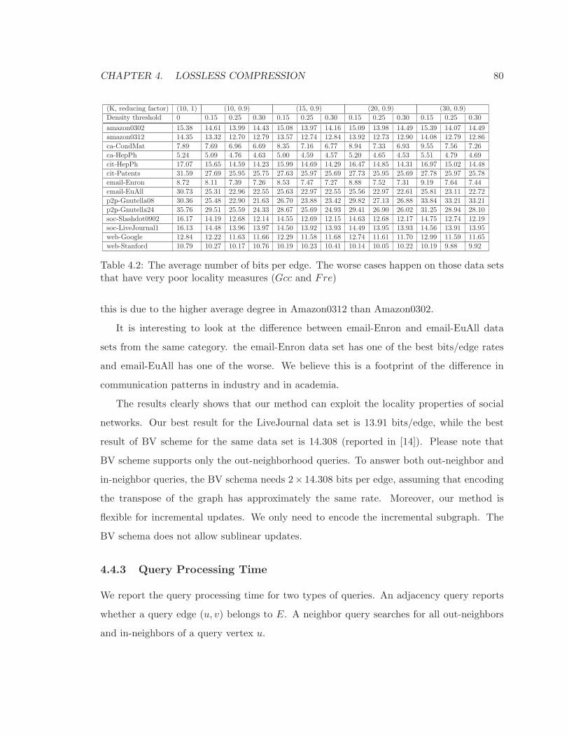
CHAPTER 4. LOSSLESS COMPRESSION 80
(K, reducing factor) (10, 1) (10, 0.9) (15, 0.9) (20, 0.9) (30, 0.9)
Density threshold 0 0.15 0.25 0.30 0.15 0.25 0.30 0.15 0.25 0.30 0.15 0.25 0.30
amazon0302 15.38 14.61 13.99 14.43 15.08 13.97 14.16 15.09 13.98 14.49 15.39 14.07 14.49
amazon0312 14.35 13.32 12.70 12.79 13.57 12.74 12.84 13.92 12.73 12.90 14.08 12.79 12.86
ca-CondMat 7.89 7.69 6.96 6.69 8.35 7.16 6.77 8.94 7.33 6.93 9.55 7.56 7.26
ca-HepPh 5.24 5.09 4.76 4.63 5.00 4.59 4.57 5.20 4.65 4.53 5.51 4.79 4.69
cit-HepPh 17.07 15.65 14.59 14.23 15.99 14.69 14.29 16.47 14.85 14.31 16.97 15.02 14.48
cit-Patents 31.59 27.69 25.95 25.75 27.63 25.97 25.69 27.73 25.95 25.69 27.78 25.97 25.78
email-Enron 8.72 8.11 7.39 7.26 8.53 7.47 7.27 8.88 7.52 7.31 9.19 7.64 7.44
email-EuAll 30.73 25.31 22.96 22.55 25.63 22.97 22.55 25.56 22.97 22.61 25.81 23.11 22.72
p2p-Gnutella08 30.36 25.48 22.90 21.63 26.70 23.88 23.42 29.82 27.13 26.88 33.84 33.21 33.21
p2p-Gnutella24 35.76 29.51 25.59 24.33 28.67 25.69 24.93 29.41 26.90 26.02 31.25 28.94 28.10
soc-Slashdot0902 16.17 14.19 12.68 12.14 14.55 12.69 12.15 14.63 12.68 12.17 14.75 12.74 12.19
soc-LiveJournal1 16.13 14.48 13.96 13.97 14.50 13.92 13.93 14.49 13.95 13.93 14.56 13.91 13.95
web-Google 12.84 12.22 11.63 11.66 12.29 11.58 11.68 12.74 11.61 11.70 12.99 11.59 11.65
web-Stanford 10.79 10.27 10.17 10.76 10.19 10.23 10.41 10.14 10.05 10.22 10.19 9.88 9.92
Table 4.2: The average number of bits per edge. The worse cases happen on those data setsthat have very poor locality measures (Gcc and Fre)
this is due to the higher average degree in Amazon0312 than Amazon0302.
It is interesting to look at the difference between email-Enron and email-EuAll data
sets from the same category. the email-Enron data set has one of the best bits/edge rates
and email-EuAll has one of the worse. We believe this is a footprint of the difference in
communication patterns in industry and in academia.
The results clearly shows that our method can exploit the locality properties of social
networks. Our best result for the LiveJournal data set is 13.91 bits/edge, while the best
result of BV scheme for the same data set is 14.308 (reported in [14]). Please note that
BV scheme supports only the out-neighborhood queries. To answer both out-neighbor and
in-neighbor queries, the BV schema needs 2× 14.308 bits per edge, assuming that encoding
the transpose of the graph has approximately the same rate. Moreover, our method is
flexible for incremental updates. We only need to encode the incremental subgraph. The
BV schema does not allow sublinear updates.
4.4.3 Query Processing Time
We report the query processing time for two types of queries. An adjacency query reports
whether a query edge (u, v) belongs to E. A neighbor query searches for all out-neighbors
and in-neighbors of a query vertex u.
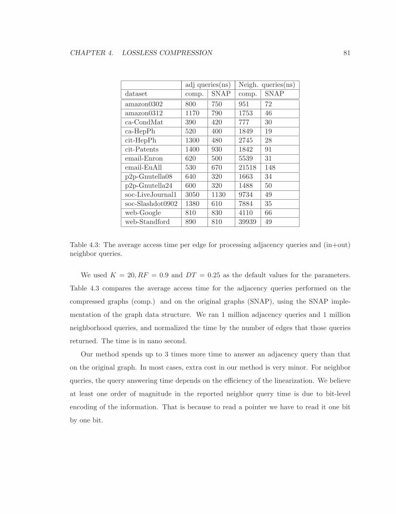
CHAPTER 4. LOSSLESS COMPRESSION 81
adj queries(ns) Neigh. queries(ns)
dataset comp. SNAP comp. SNAP
amazon0302 800 750 951 72
amazon0312 1170 790 1753 46
ca-CondMat 390 420 777 30
ca-HepPh 520 400 1849 19
cit-HepPh 1300 480 2745 28
cit-Patents 1400 930 1842 91
email-Enron 620 500 5539 31
email-EuAll 530 670 21518 148
p2p-Gnutella08 640 320 1663 34
p2p-Gnutella24 600 320 1488 50
soc-LiveJournal1 3050 1130 9734 49
soc-Slashdot0902 1380 610 7884 35
web-Google 810 830 4110 66
web-Standford 890 810 39939 49
Table 4.3: The average access time per edge for processing adjacency queries and (in+out)neighbor queries.
We used K = 20, RF = 0.9 and DT = 0.25 as the default values for the parameters.
Table 4.3 compares the average access time for the adjacency queries performed on the
compressed graphs (comp.) and on the original graphs (SNAP), using the SNAP imple-
mentation of the graph data structure. We ran 1 million adjacency queries and 1 million
neighborhood queries, and normalized the time by the number of edges that those queries
returned. The time is in nano second.
Our method spends up to 3 times more time to answer an adjacency query than that
on the original graph. In most cases, extra cost in our method is very minor. For neighbor
queries, the query answering time depends on the efficiency of the linearization. We believe
at least one order of magnitude in the reported neighbor query time is due to bit-level
encoding of the information. That is because to read a pointer we have to read it one bit
by one bit.
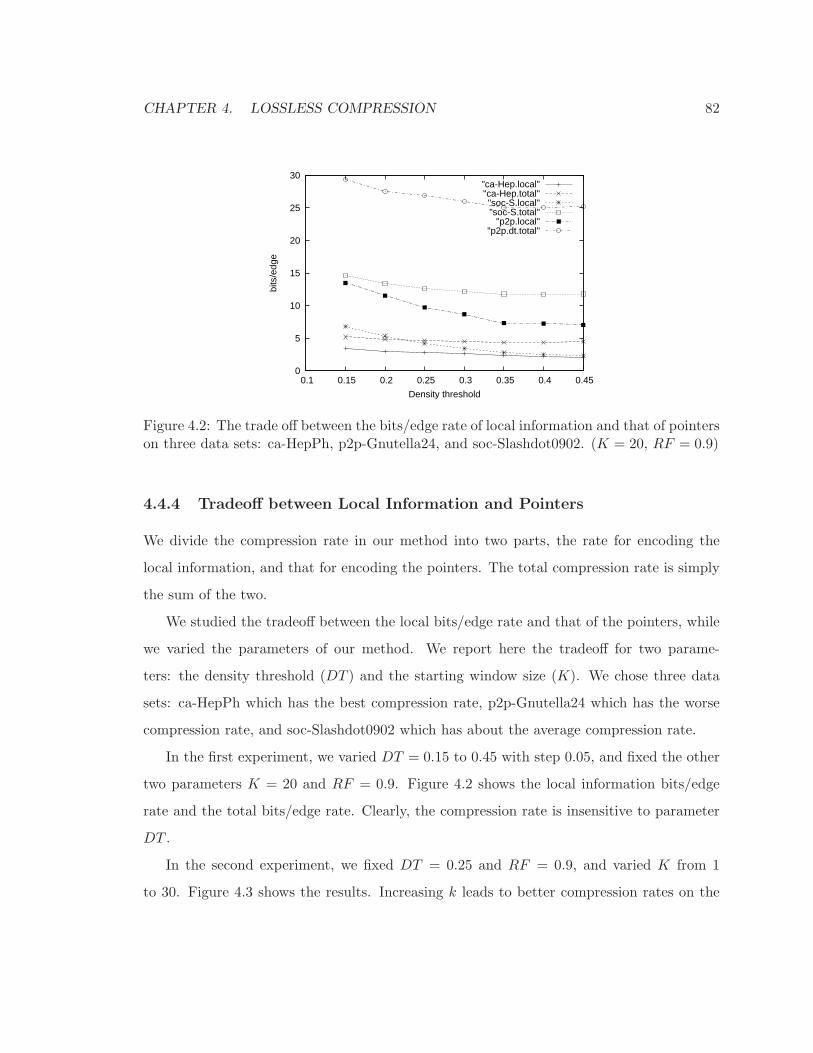
CHAPTER 4. LOSSLESS COMPRESSION 82
0
5
10
15
20
25
30
0.1 0.15 0.2 0.25 0.3 0.35 0.4 0.45
bits
/edg
e
Density threshold
"ca-Hep.local""ca-Hep.total""soc-S.local""soc-S.total"
"p2p.local""p2p.dt.total"
Figure 4.2: The trade off between the bits/edge rate of local information and that of pointerson three data sets: ca-HepPh, p2p-Gnutella24, and soc-Slashdot0902. (K = 20, RF = 0.9)
4.4.4 Tradeoff between Local Information and Pointers
We divide the compression rate in our method into two parts, the rate for encoding the
local information, and that for encoding the pointers. The total compression rate is simply
the sum of the two.
We studied the tradeoff between the local bits/edge rate and that of the pointers, while
we varied the parameters of our method. We report here the tradeoff for two parame-
ters: the density threshold (DT ) and the starting window size (K). We chose three data
sets: ca-HepPh which has the best compression rate, p2p-Gnutella24 which has the worse
compression rate, and soc-Slashdot0902 which has about the average compression rate.
In the first experiment, we varied DT = 0.15 to 0.45 with step 0.05, and fixed the other
two parameters K = 20 and RF = 0.9. Figure 4.2 shows the local information bits/edge
rate and the total bits/edge rate. Clearly, the compression rate is insensitive to parameter
DT .
In the second experiment, we fixed DT = 0.25 and RF = 0.9, and varied K from 1
to 30. Figure 4.3 shows the results. Increasing k leads to better compression rates on the
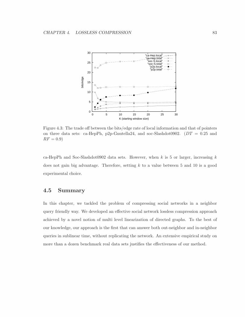
CHAPTER 4. LOSSLESS COMPRESSION 83
0
5
10
15
20
25
30
0 5 10 15 20 25 30
bits
/edg
e
K (starting window size)
"ca-Hep.local""ca-Hep.total""soc-S.local""soc-S.total"
"p2p.local""p2p.total"
Figure 4.3: The trade off between the bits/edge rate of local information and that of pointerson three data sets: ca-HepPh, p2p-Gnutella24, and soc-Slashdot0902. (DT = 0.25 andRF = 0.9)
ca-HepPh and Soc-Slashdot0902 data sets. However, when k is 5 or larger, increasing k
does not gain big advantage. Therefore, setting k to a value between 5 and 10 is a good
experimental choice.
4.5 Summary
In this chapter, we tackled the problem of compressing social networks in a neighbor
query friendly way. We developed an effective social network lossless compression approach
achieved by a novel notion of multi level linearization of directed graphs. To the best of
our knowledge, our approach is the first that can answer both out-neighbor and in-neighbor
queries in sublinear time, without replicating the network. An extensive empirical study on
more than a dozen benchmark real data sets justifies the effectiveness of our method.
Chapter 5
Lossy Compression
From both practical and theoretical points of views, compression plays an important role
in social network analysis. Although there are a few pioneering studies on social network
compression [9, 4, 52], they only focus on lossless approaches. In this chapter, we tackle
the problem of lossy compression of social networks. The trade-off between memory and
“information-preserved” in a lossy compression presents an interesting angle for social net-
work analysis, and at the same time makes the problem very challenging. We propose a
lossy graph compression approach, based on our GPSN framework. We do so by design-
ing an objective function to measure the quality of a given linearization with respect to
community structure of social networks. We present an interesting and practical greedy
algorithm to optimize such an objective function. Our experimental results on real data
sets and synthetic data sets demonstrate the promise of our method.
5.1 Overview
Partly motivated by the recent success of many online social networking sites such as Face-
book and Twitter, managing and analyzing huge social networks have attracted dramatic
interest from both industry and academia. An essential challenge is that many social net-
works are huge and ever growing. For example, from January to September 2008, the
84
CHAPTER 5. LOSSY COMPRESSION 85
number of active users of Facebook grew from 60 million to 140 million, and Facebook has
over 900 million active users nowadays.
As illustrated by several recent studies [8, 14, 40, 6], compressing social networks can
substantially facilitate mining and advanced analysis of huge social networks. Social network
compression plays an important role in social network analysis from both practical and
theoretical points of view.
Practically, many advanced social network analysis tools are sensitive to the input size.
Those methods are highly efficient when the data can be held completely or largely into
main memory, but are very costly if most of the data is out of memory. If social networks
can be compressed effectively and efficiently, it may help such advanced analysis tools to
handle much larger social networks.
Theoretically, compression is always achieved by utilizing some local “regularity” in
data. Thus, the compressibility of a social network can provide valuable insights into the
structure of the network. For example, if a subnetwork can be compressed well, it may
indicate that the members in the subnetwork share some regularity, or the subnetwork
follows some structural patterns that are shared by similar subnetworks.
As indicated by a literature review in Chapter 2, almost all the existing social network
compression methods target at lossless compression. We argue that lossy compression in
fact is very interesting and useful for social networks, because it is well-known that large
social networks are often noisy.
From the practical point of view, noise edges and vertices in large social networks may
hinder the quality of social network analysis. An appropriate lossy compression of a social
network should discard the noise edges and vertices in the network. Consequently, the lossy
compression may be present as the input of higher quality for social network analysis. In
other words, lossy compression of social networks can serve as a preprocessing step in social
network analysis. This goes far beyond just space saving.
From the theoretical point of view, lossy compression of social networks can help to dis-
cover the importance of edges and vertices in a social network, and identify noise edges and
CHAPTER 5. LOSSY COMPRESSION 86
vertices. Suppose ideally we have a lossy compression method that preserves the important
information about a social network and filters out noise. If the method can assign to each
element in a social network (e.g., each edge and vertex) a priority of being included into a
lossy compression, then the priority can be regarded as a good indicator of the importance
of the element. The lower the priority of an element, the more likely the element is noise.
Lossy compression of social networks is interesting and important for social network
analysis. At the same time, it is a very challenging problem. To achieve good lossy com-
pression of social networks, we have to develop good methodology that can detect and
preserve important information in social networks.
In this chapter, we tackle the novel problem of community preserving lossy compression
of social networks, and make several important contributions. First, we advocate community
preserving lossy compression of social networks due to the importance of communities in
social networks. To the best of our knowledge, we are the first to identify and tackle the
problem. Second, we propose a sequence graph compression approach. We design a simple
yet meaningful objective function that optimizes for community structure preservation. We
are not aware of any other objective function for the same purpose in the literature. A
heuristic algorithm is developed. Last, we report an empirical study on both synthetic and
real data sets, which verifies the effectiveness of our method.
The rest of the chapter is organized as follows. In Section 5.2, the notations and the
essential idea of our compression method using the GPSN framework is discussed. The
design of the community preserving objective function is covered in Section 5.3. We present
the compression algorithm in Section 5.4, and report the experimental results in Section 5.5.
Section 5.6 summarizes the chapter.
5.2 Graph Linearization for Lossy Compression
For the sake of simplicity, in this chapter, we model a social network as an undirected simple
graph G = (V,E), where V is a set of vertices, E ⊂ V × V is a set of edges, and (u, u) 6∈ Efor any u ∈ V . We also refer to V by V (G) and to E by E(G). Our discussion can be

CHAPTER 5. LOSSY COMPRESSION 87
straightforwardly extended to directed and non-simple graphs.
We first formulate a notion of sequence graph.
Definition 12 (Sequence graph). A graph Gs is a (k, l)-sequence graph, if |V (Gs)| = l
and there is a bijection φ between V (Gs) and the set of integers {1, . . . , l} such that for every
edge (x, y) ∈ E(Gs), |φ(x) − φ(y)| ≤ k. We call k the local range size, l the sequence
length, and span(x, y) = |φ(x)− φ(y)| the span of edge (x, y).
Intuitively, in a sequence graph, the vertices can be lined up into a sequence so that all
edges are “local”, that is, the two end points locate within a segment of at most k in the
sequence. Since φ is a bijection between V (Gs) and integers {1, . . . , l}, hereafter, we may
simply refer to the vertices in Gs by integers in {1, . . . , l}, and may draw the vertices of a
sequence graph in a sequence and omit the integers if they are clear from the context.
Example 9 (Sequence graph). Graph Gs in Figure 5.1(b) is a (3, 15)-sequence graph. Please
note that we simply line up the vertices in a sequence and omit the integers in the graph.
The function ψ(·) in the figure is for Example 10 and should be ignored at this moment.
To store a (k, l)-sequence graph, for each vertex, we only need to allocate 2k bits to
represent the edges involving the vertex. This representation can also enable efficient neigh-
borhood queries — finding all neighbors of a vertex u takes only O(k) time.
The general idea behind graph compression using linearization is that we try to “unfold”
a graph into a sequence graph, so that many vertices have the associated edges in their local
ranges. Then, storing the corresponding sequence graph can save space, because many
edges are stored using only 2 bits each, one for each end point. We refer to this process as
“unfolding” because a vertex in the original graph may be mapped to several vertices in the
sequence graph.
Definition 13 (Graph linearization). A (k, l)-sequence graph Gs is a (k, l)-linearization
of a graph G if there exists a function ψ : V (Gs) → V (G) such that (1) for every edge
(x, y) ∈ E(Gs), (ψ(x), ψ(y)) ∈ E(G), and (2) there does not exist two edges (x, y), (x′, y′) ∈
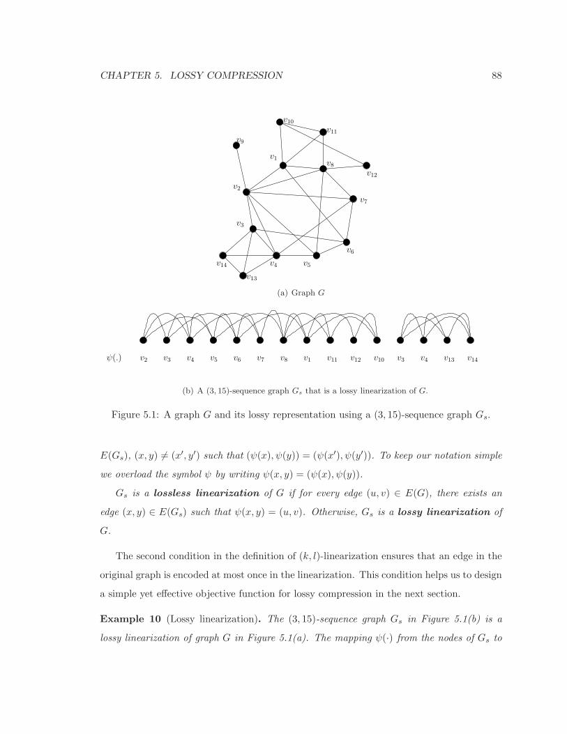
CHAPTER 5. LOSSY COMPRESSION 88
v3
v5
v6
v7
v8
v2
v1
v12
v10
v9
v11
v4
v13
v14
(a) Graph G
v3 v4 v13 v14ψ(.) v2 v3 v4 v5 v6 v7 v8 v1 v11 v12 v10
(b) A (3, 15)-sequence graph Gs that is a lossy linearization of G.
Figure 5.1: A graph G and its lossy representation using a (3, 15)-sequence graph Gs.
E(Gs), (x, y) 6= (x′, y′) such that (ψ(x), ψ(y)) = (ψ(x′), ψ(y′)). To keep our notation simple
we overload the symbol ψ by writing ψ(x, y) = (ψ(x), ψ(y)).
Gs is a lossless linearization of G if for every edge (u, v) ∈ E(G), there exists an
edge (x, y) ∈ E(Gs) such that ψ(x, y) = (u, v). Otherwise, Gs is a lossy linearization of
G.
The second condition in the definition of (k, l)-linearization ensures that an edge in the
original graph is encoded at most once in the linearization. This condition helps us to design
a simple yet effective objective function for lossy compression in the next section.
Example 10 (Lossy linearization). The (3, 15)-sequence graph Gs in Figure 5.1(b) is a
lossy linearization of graph G in Figure 5.1(a). The mapping ψ(·) from the nodes of Gs to

CHAPTER 5. LOSSY COMPRESSION 89
Symbol Meaning
Gs a (k, l)-sequence graphG a graph to be compressedk the neighbor range sizel the sequence lengthφ the mapping between V (Gs) and the
set of integers {1, . . . , l}span(x, y) the span of edge (x, y) ∈ E(Gs), |φ(x)−
φ(y)|Ns(x) the neighbor set of x, {y ∈
V (Gs)||φ(x)− φ(y)| ≤ k}ψ the mapping from V (Gs) to V (G) in a
linearizationψ(x, y) (ψ(x), ψ(y))p a path
span(p) the span of a path in Gs,max1≤i≤m{φ(u′i)} −min1≤i≤m{φ(u′i)}
Pm(Gs) the set of length-m paths in Gs
Table 5.1: Some frequently used notions.
the nodes of G is depicted.
In general, a graph G may have multiple (k, l)-lossy linearizations. Finding the best
(k, l)-lossy linearization for a graph G is a novel problem not touched by any previous work.
To make the problem concrete, we need to explore how to quantify the “loss of information”
and assess the degree of community preservation in lossy compression. We answer this
question by designing an objective function in the next section.
The frequently used notions are summarized in Table 5.1.
5.3 Objective Function
Consider the following optimization problem. Given a graph G and parameters l > 0 and
k > 0, find a (k, l)-lossy linearization Gs for G and the mapping ψ : V (Gs) → V (G) such
that a utility objective function f(Gs) is maximized, where f(Gs) measures the degree of
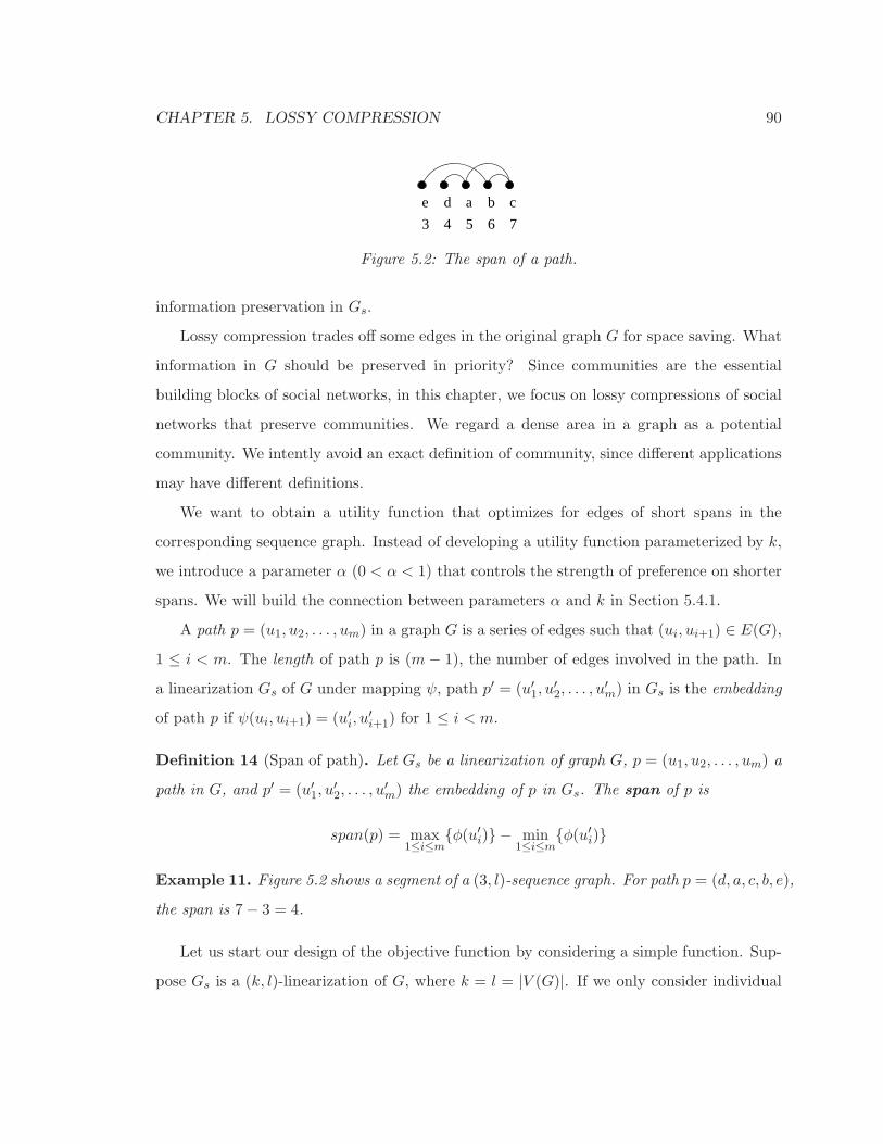
CHAPTER 5. LOSSY COMPRESSION 90
7
a b cde
3 4 5 6
Figure 5.2: The span of a path.
information preservation in Gs.
Lossy compression trades off some edges in the original graph G for space saving. What
information in G should be preserved in priority? Since communities are the essential
building blocks of social networks, in this chapter, we focus on lossy compressions of social
networks that preserve communities. We regard a dense area in a graph as a potential
community. We intently avoid an exact definition of community, since different applications
may have different definitions.
We want to obtain a utility function that optimizes for edges of short spans in the
corresponding sequence graph. Instead of developing a utility function parameterized by k,
we introduce a parameter α (0 < α < 1) that controls the strength of preference on shorter
spans. We will build the connection between parameters α and k in Section 5.4.1.
A path p = (u1, u2, . . . , um) in a graph G is a series of edges such that (ui, ui+1) ∈ E(G),
1 ≤ i < m. The length of path p is (m − 1), the number of edges involved in the path. In
a linearization Gs of G under mapping ψ, path p′ = (u′1, u′2, . . . , u
′m) in Gs is the embedding
of path p if ψ(ui, ui+1) = (u′i, u′i+1) for 1 ≤ i < m.
Definition 14 (Span of path). Let Gs be a linearization of graph G, p = (u1, u2, . . . , um) a
path in G, and p′ = (u′1, u′2, . . . , u
′m) the embedding of p in Gs. The span of p is
span(p) = max1≤i≤m
{φ(u′i)} − min1≤i≤m
{φ(u′i)}
Example 11. Figure 5.2 shows a segment of a (3, l)-sequence graph. For path p = (d, a, c, b, e),
the span is 7− 3 = 4.
Let us start our design of the objective function by considering a simple function. Sup-
pose Gs is a (k, l)-linearization of G, where k = l = |V (G)|. If we only consider individual

CHAPTER 5. LOSSY COMPRESSION 91
edges, and try to decrease the sum of spans of all edges, then we have the following utility
function:
f1(Gs) =∑
(x,y)∈E(Gs)
αspan(x,y)
Utility function f1 has the following two properties.
Property 1: the shorter the spans of edges in the sequence graph, the higher the utility.
This property is consistent with our goal of preserving community information. A com-
munity typically has a high density, which means there exist many edges among the set of
vertices belonging to the community. If the vertices of a community are placed in proximate
positions in the sequence, the spans of the edges within the community tend to be short.
The edges of long spans contribute little to the utility. The utility decreases exponentially
with respect to the span. This property encourages the arrangement of vertices belonging
to the same community in the close-by positions, and discourages the inclusion of edges
crossing communities far away in the original graph G.
Property 2: the more edges included in the compression, the higher the utility. Consider
two linearization graphs Gs and G′s such that V (Gs) = V (G′
s) and E(Gs) ⊂ E(G′s). Then,
f1(Gs) < f1(G′s). This property encourages a linearization graph to include as many edges
as possible in addition to optimizing for short span edges.
Utility function f1 is sensitive to individual edges. We can extend it to incorporate
community information better. Instead of edges, we can consider how paths of a certain
length are represented in a sequence graph. Generally, a community as a dense subgraph has
many short paths traversing members within the community. If a sequence graph preserves
the community information, then the members of the community are lined up close to one
another in the sequence graph and thus the paths in the community fall into short ranges
of the sequence.
To incorporate the above idea, let Pm(Gs) be the set of paths of length m in a sequence
graph Gs. We can extend utility function f1 to
fm(Gs) =∑
p∈Pm(Gs)
αspan(p)
CHAPTER 5. LOSSY COMPRESSION 92
Clearly, utility function fm is a generalization of f1. The longer the paths considered, the
more community oriented the utility function becomes. At the same time, the optimization
problem becomes more challenging when the value of m increases.
Observe that the function f1 takes its maximum value when the span of each edge is one,
and that is basically an adjacency representation of the graph. In this chapter, we focus on
the simplest nontrivial setting m = 2 as the first step. Interestingly, several recent studies,
such as [28], suggested that even considering random walks of short length can generate high
quality results in network analysis. Note that for m ≥ 3, the problem is computationally
more expensive. Optimizing fm for larger values of m is the subject of future studies.
For the sake of simplicity, we omit the subscript 2. In the rest of the chapter, we tackle
the optimization of the following objective function:
f(Gs) = f2(Gs) =∑
p∈P2(Gs)
αspan(p) (5.1)
5.4 Linearization Method
In this section, we simplify the objective function, build the connection between parameters
α and k, and develop a greedy heuristic linearization method.
How difficult is the problem of finding the optimal lossy linearization using utility func-
tion f in Equation 5.1, that is, finding a sequence graph maximizing the objective function?
In literature, there is a family of graph layout problems [19], whose objective is to find an or-
dering of nodes to optimize a particular objective function. Many variants of these problems
have been shown to be NP-hard [47, 14]. To the best of our knowledge, even no constant
factor approximation algorithm for any variation of these problems is known [59, 19]. Note
that our setting is even more complex, since one node can appear in several positions in
a sequence graph. These evidences suggest that very likely the problem is not solvable in
polynomial time, unless P = NP . Therefore, in this section, we design a greedy heuristic
method.
In order to obtain effective greedy heuristics, we try to bound the objective function.
We observe the following.
CHAPTER 5. LOSSY COMPRESSION 93
Theorem 2 (Bounds). Let Gs be a sequence graph. Then,
f(Gs) ≤∑
p∈P2(Gs)
(α1/2)span(e1)+span(e2) (5.2)
f(Gs) ≥∑
p∈P2(Gs)
αspan(e1)+span(e2) (5.3)
Proof. For any path p = e1e2 in Gs, we have span(p) ≥ max{span(e1), span(e2)} ≥span(e1)+span(e2)
2 . Since 0 < α < 1, Equation 5.2 follows immediately.
Apparently, span(p) ≤ span(e1) + span(e2). Thus, Equation 5.3 holds.
Heuristically, if we can obtain a sequence graph optimizing the lower bound in Theo-
rem 2, the sequence graph have a good chance to boost the objective function f . Note that,
optimizing the lower bound in Theorem 2 is computationally less expensive.
Let Ei be the set of edges incident to vertex i in Gs and Pi be the set of those paths of
length two that have vertex i as the middle vertex. Then,
(∑
e∈Ei
αspan(e))2 =∑
p=e1e2∈Pi
αspan(e1)+span(e2)
The equation holds, because after expanding the left side, for any possible pair of edges e1
and e2 in Ei, we have the term αspan(e1)+span(e2). Moreover, each possible pair of edges in
Ei is corresponding to a path in Pi, and vice versa. Therefore, we optimize the lower bound
in Theorem 2 if we optimize the following nice double summation:
f(Gs) =∑
1≤i≤|V (Gs)|
(∑
e∈Ei
αspan(e))2
5.4.1 Connection between Parameters α and k
We have the following interesting upper bound for the span of any given edge in the optimal
sequence graph, assuming the value of α is given.
Theorem 3. For a given α, the maximum span of all edges in the optimal sequence graph
is at most logαα(1−α)
4 .
CHAPTER 5. LOSSY COMPRESSION 94
Proof. Let wi =∑
e∈Eiαspan(e), where Ei is the set of edges associated with position i.
wi =∑
e∈Ei
αspan(e) < 2∞∑
t=1
αt
Notice that, in Ei, there are at most two edges with span equal to t for any possible t.
However,∑∞
t=1 αt is the sum of a geometric sequence and is equal to α/(1 − α). Thus we
can rewrite the inequality in the following form:
wi <2α
1− α
The contribution of edge e is at most:
w2i − (wi − αspan(e))2 = 2αspan(e)wi − α2span(e)
<4αspan(e)+1
1− α − α2span(e)
This value should be larger than the contribution of a single isolated edge, otherwise
removing this edge and adding it to the end of the sequence graph would increase the
objective function. Thus,
α2 <4αspan(e)+1
1− α − α2span(e)
α(1− α)4
<α2(1− α)
4α− αspan(e)(1− α) < αspan(e)
Since 0 < α < 1 and span(e) is an integer, we have
span(e) < logαα(1− α)
4
Our problem formulation assumes a parameter k is given as the maximum local range size
for the sequence graph. However, the objective function uses the parameter α. Theorem 3
builds the analytical ground to connect α with k. We use the equation k = logαα(1−α)
4 to
estimate α. Specifically, to estimate α given k, we do a binary search on the interval [0, 1],
and stop when the value of logαα(1−α)
4 is between k and k− 0.01. Using this estimate of α,
experimentally we observe that in the resulting sequence graphs the spans of an extremely
small fraction of edges are more than k/2. This is consistent with Theorem 3. Therefore,
we use the equation 2k = logα(1− α)α/4 to estimate α.

CHAPTER 5. LOSSY COMPRESSION 95
Algorithm 7 Compression Algorithm
Input: G: input network, k: local range,l: length of compression (l ≥ |V (G)|)
Output: SeqG: sequenced compression1: Initialize SeqG with a random ordering of nodes2: α← EstimateAlpha(k)3: repeat4: b = f(SeqG, α)5: for all u ∈ V (G) do6: IPos = NULL, DPos = NULL7: (IPos,Nbh)← ReAllocate(u,G, SeqG, α)8: if (IPos 6= NULL) and (Length(SeqG) = l) then9: DPos← SeqG.LowestBenf(IPos− k, IPos+ k)
10: end if11: x← UtilityIncrease(IPos,Nbh, SeqG)12: y ← UtilityDecrease(DPos, SeqG)13: if x− y > 0 then14: Insert(IPos,Nbh, SeqG)15: Delete(DPos, SeqG)16: end if17: end for18: a = f(SeqG, α)19: until convergence condition
5.4.2 A Greedy Heuristic Method
In this section, we develop a greedy heuristic method for the community preserving lossy
compression problem. We will use a local search heuristic.
Overview and General Ideas
The basic operation for local improvement in our heuristic is that, given a node, we find a
position in the sequence to insert a new copy of the node, and find a position to delete such
that the total change in the objective function is positive after the insertion and deletion.
Similar to most local search heuristic methods, our method does not have any theoretical
guarantee for the convergence time or the quality of the result. However, using an extensive
set of experiments in the next section we verify the effectiveness of our design in practice.
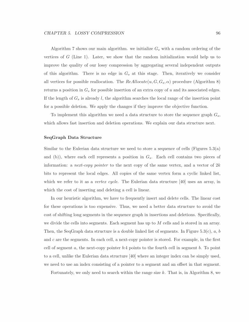
CHAPTER 5. LOSSY COMPRESSION 96
Algorithm 7 shows our main algorithm. we initialize Gs with a random ordering of the
vertices of G (Line 1). Later, we show that the random initialization would help us to
improve the quality of our lossy compression by aggregating several independent outputs
of this algorithm. There is no edge in Gs at this stage. Then, iteratively we consider
all vertices for possible reallocation. The ReAllocate(u,G,Gs, α) procedure (Algorithm 8)
returns a position in Gs for possible insertion of an extra copy of u and its associated edges.
If the length of Gs is already l, the algorithm searches the local range of the insertion point
for a possible deletion. We apply the changes if they improve the objective function.
To implement this algorithm we need a data structure to store the sequence graph Gs,
which allows fast insertion and deletion operations. We explain our data structure next.
SeqGraph Data Structure
Similar to the Eulerian data structure we need to store a sequence of cells (Figures 5.3(a)
and (b)), where each cell represents a position in Gs. Each cell contains two pieces of
information: a next-copy pointer to the next copy of the same vertex, and a vector of 2k
bits to represent the local edges. All copies of the same vertex form a cyclic linked list,
which we refer to it as a vertex cycle. The Eulerian data structure [40] uses an array, in
which the cost of inserting and deleting a cell is linear.
In our heuristic algorithm, we have to frequently insert and delete cells. The linear cost
for these operations is too expensive. Thus, we need a better data structure to avoid the
cost of shifting long segments in the sequence graph in insertions and deletions. Specifically,
we divide the cells into segments. Each segment has up to M cells and is stored in an array.
Then, the SeqGraph data structure is a double linked list of segments. In Figure 5.3(c), a, b
and c are the segments. In each cell, a next-copy pointer is stored. For example, in the first
cell of segment a, the next-copy pointer b:4 points to the fourth cell in segment b. To point
to a cell, unlike the Eulerian data structure [40] where an integer index can be simply used,
we need to use an index consisting of a pointer to a segment and an offset in that segment.
Fortunately, we only need to search within the range size k. That is, in Algorithm 8, we
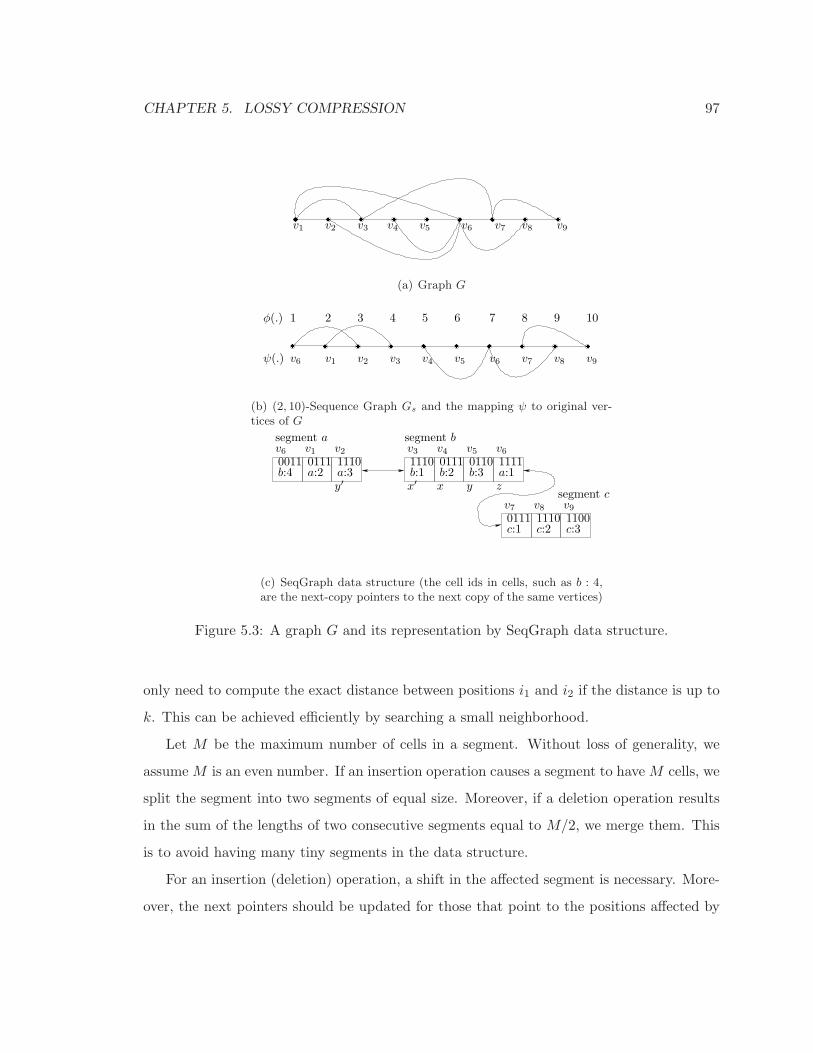
CHAPTER 5. LOSSY COMPRESSION 97
���� ���� ���� �������� ���� �� ���� ����
v1 v2 v3 v4 v5 v6 v7 v8 v9
(a) Graph G
��������
��������
��������
��������
��������
��������
����
��������
��������
��
ψ(.)
φ(.) 1
v6 v6
2
v1
3 4 5 6 7 8 9 10
v2 v3 v4 v5 v7 v8 v9
(b) (2, 10)-Sequence Graph Gs and the mapping ψ to original ver-tices of G
b:40011 0111 1110 1110 0111 0110 1111
0111 1110 1100
a:2 a:3 b:1 b:2 b:3 a:1
c:1 c:2 c:3
x y zx′y′
segment a segment b
segment c
v6 v6v1 v2 v3 v4 v5
v7 v8 v9
(c) SeqGraph data structure (the cell ids in cells, such as b : 4,are the next-copy pointers to the next copy of the same vertices)
Figure 5.3: A graph G and its representation by SeqGraph data structure.
only need to compute the exact distance between positions i1 and i2 if the distance is up to
k. This can be achieved efficiently by searching a small neighborhood.
Let M be the maximum number of cells in a segment. Without loss of generality, we
assumeM is an even number. If an insertion operation causes a segment to haveM cells, we
split the segment into two segments of equal size. Moreover, if a deletion operation results
in the sum of the lengths of two consecutive segments equal to M/2, we merge them. This
is to avoid having many tiny segments in the data structure.
For an insertion (deletion) operation, a shift in the affected segment is necessary. More-
over, the next pointers should be updated for those that point to the positions affected by

CHAPTER 5. LOSSY COMPRESSION 98
the insertion and deletion, that is, the position of insertion or deletion and the positions
thereafter in the same segment. A nice property of our SeqGraph data structure is that all
other segments are not affected. Finally, those edges that pass over the insertion (deletion)
position should be updated, too.
Example 12. In Figure 5.3(c), let us call the cells b:2, b:3 and b:4, x, y and z, respectively,
as labeled in the figure. To insert a copy of v7 at position b:2, a shift in the segment b is
needed. Moreover, we have to change the next-copy pointers of all the cells that point to x,
y and z to b:3, b:4 and b:5, respectively. Note that we can find these pointers by following
the vertex cycles of x, y and z, respectively. The edges associated with those cells that are
at most 2 positions away from the inserted cell should be updated, that is x, x′, y and y′.
Finally, the newly inserted cell should be added to the vertex cycle of v7.
The cost of the insertion and deletion operations depends on the sizes of segments,
vertex cycles and maximum span of edges. The time complexity of an insertion or deletion
operation is O(M∆+ k2), where ∆ is the maximum degree of the graph.
The Reallocation Procedure
For a node u, the reallocation procedure (Algorithm 8) partitions the edges incident to u
into groups. Each group is associated with a copy of u in Gs. Let C1 be the set of positions
of copies of u that already exist in Gs, and C2 be the set of positions of potential new copies.
C2 is generated as follows: let E(G \ Gs) be the set of edges (u, v) ∈ E(G) that are not
represented in Gs. For (u, v) ∈ E(G \Gs), we add a potential new copy of u right behind a
random copy of v in Gs (Lines 3-7).
We insert these new potential copies at the beginning, and delete them all at the end of
the procedure (Lines 1-12). In the edge reassigning step (Lines 13-26), each edge is added
to the group for which it has the best contribution (Line 19). The reassigning process stops
when no improvement is possible. At the end, for the existing copies of u, that is, C1,
the associated edges will be updated if they have been changed (Lines 27-29). For those
potential new copies, that is, C2, we remove them and return the best in the set as the

CHAPTER 5. LOSSY COMPRESSION 99
position of a potential new copy of u in Gs. We also return the edges associated to this
potential new copy (Lines 30-35).
Running Time Analysis
Let dv be the degree of node v. We have at most dv groups for each vertex. Inserting and
deleting the groups in the SeqGraph data structure takes O(dv(M∆ + k2)) time. In an
iteration of the edge reassigning process, all edges have to be considered for reassigning.
Each edge takes O(dvk) time. In total each iteration takes O(d2vk) time.
We notice that the number of iteration in practice is extremely low, typically 2 or 3.
We do not have any theoretical bound on the number of iterations. However, since the
contribution of any single edge is increasing, the convergence is guaranteed.
Likewise, the overall time complexity of Algorithm 7 depends on the convergence con-
dition and the number of iterations. However, the complexity of a single iteration can be
estimated as follows. Assuming the number of iterations for the reallocation process is at
most I, the running time is proportional to∑
v∈V (G) dv(dvkI +M∆+ k2). Since k and M
are constants, the sum is proportional to∑
v∈V (G) dv(dvI + ∆). Notice that dv is at most
∆, therefore, the time complexity of an iteration is O(|E|∆I).
5.5 Empirical Evaluation
In this section, we report a systematic empirical evaluation.
5.5.1 Evaluation Methodology
Our compression algorithm assumes the parameters k, the local range size, and l, the length
of linearization, are given. Having these parameters fixed, the size of compression can be
computed precisely. Therefore, compression rate does not have a straightforward meaning
here. Instead, we consider a measure to assess the utility of a single bit.
Definition 15 (Bit-utility rate). The bit-utility rate is the ratio of the number of edges
encoded in the lossy compression over the total number of bits.
CHAPTER 5. LOSSY COMPRESSION 100
To evaluate the quality of a lossy compression, one has to look at the quality of com-
munity preservation. This is a challenging task. It is hard to find a ground truth for the
community structure of real world networks. Moreover, our method does not explicitly
identify communities of networks.
For a sanity check of our method, we design the following methodology. Using the
distance of the vertices in the sequence graph compression, we define a proximity graph
(Definition 16), which is a weighted graph on the vertex set of the original network. The
weight of edge (u, v) is an indicator for u and v belonging to the same community. Then, we
run a simple community structure detection algorithm on both the original network and the
proximity graph. A significant improvement in community detection should be interpreted
as the effectiveness of our community preservation lossy compression method. To have a
ground truth, we use synthesis networks with implanted communities.
The second experiment is concerned with the effect of missing edges in the lossy com-
pression. We compare three different centrality measures on both the network with the
original set of edges and the network with the set of those edges that are encoded in the
compressed version. We use a collection of real world networks for this experiment.
5.5.2 Synthesis Networks
The LFR [35] benchmark is a random model to generate networks with implanted commu-
nities of variable size, while the degree of the nodes follows a power law distribution. We
use the algorithm by Clauset et al. [16] for detecting the community structure. This is a
simple and scalable greedy modularity-based algorithm. As reported by Fortunato [27] in
his Figure 33, this algorithm has a poor performance on the LFR benchmark. A significant
improvement of the performance of this algorithm over our lossy representation of the net-
work supports our claim that our method is more than a compression framework and can
serve as a preprocessing step for clustering analysis.
To generate synthesis networks, we use the same settings as those used by Fortunato [27].
We set the parameters as follows: average degree to 20, maximum degree to 50, exponent
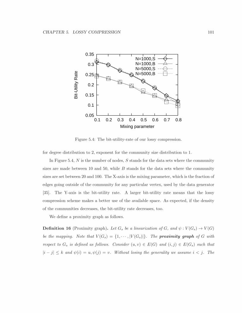
CHAPTER 5. LOSSY COMPRESSION 101
0.05
0.1
0.15
0.2
0.25
0.3
0.35
0.1 0.2 0.3 0.4 0.5 0.6 0.7 0.8
Bit-
Util
ity R
ate
Mixing parameter
N=1000,SN=1000,BN=5000,SN=5000,B
Figure 5.4: The bit-utility-rate of our lossy compression.
for degree distribution to 2, exponent for the community size distribution to 1.
In Figure 5.4, N is the number of nodes, S stands for the data sets where the community
sizes are made between 10 and 50, while B stands for the data sets where the community
sizes are set between 20 and 100. The X-axis is the mixing parameter, which is the fraction of
edges going outside of the community for any particular vertex, used by the data generator
[35]. The Y-axis is the bit-utility rate. A larger bit-utility rate means that the lossy
compression scheme makes a better use of the available space. As expected, if the density
of the communities decreases, the bit-utility rate decreases, too.
We define a proximity graph as follows.
Definition 16 (Proximity graph). Let Gs be a linearization of G, and ψ : V (Gs)→ V (G)
be the mapping. Note that V (Gs) = {1, · · · , |V (Gs)|}. The proximity graph of G with
respect to Gs is defined as follows. Consider (u, v) ∈ E(G) and (i, j) ∈ E(Gs) such that
|i − j| ≤ k and ψ(i) = u, ψ(j) = v. Without losing the generality we assume i < j. The
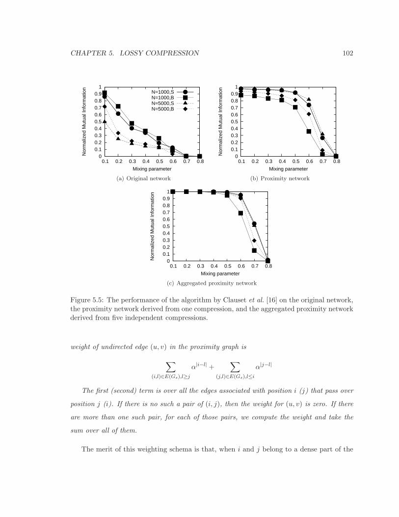
CHAPTER 5. LOSSY COMPRESSION 102
0 0.1 0.2 0.3 0.4 0.5 0.6 0.7 0.8 0.9
1
0.1 0.2 0.3 0.4 0.5 0.6 0.7 0.8
Nor
mal
ized
Mut
ual I
nfor
mat
ion
Mixing parameter
N=1000,SN=1000,BN=5000,SN=5000,B
(a) Original network
0 0.1 0.2 0.3 0.4 0.5 0.6 0.7 0.8 0.9
1
0.1 0.2 0.3 0.4 0.5 0.6 0.7 0.8
Nor
mal
ized
Mut
ual I
nfor
mat
ion
Mixing parameter
(b) Proximity network
0 0.1 0.2 0.3 0.4 0.5 0.6 0.7 0.8 0.9
1
0.1 0.2 0.3 0.4 0.5 0.6 0.7 0.8
Nor
mal
ized
Mut
ual I
nfor
mat
ion
Mixing parameter
(c) Aggregated proximity network
Figure 5.5: The performance of the algorithm by Clauset et al. [16] on the original network,the proximity network derived from one compression, and the aggregated proximity networkderived from five independent compressions.
weight of undirected edge (u, v) in the proximity graph is
∑
(i,l)∈E(Gs),l≥j
α|i−l| +∑
(j,l)∈E(Gs),l≤i
α|j−l|
The first (second) term is over all the edges associated with position i (j) that pass over
position j (i). If there is no such a pair of (i, j), then the weight for (u, v) is zero. If there
are more than one such pair, for each of those pairs, we compute the weight and take the
sum over all of them.
The merit of this weighting schema is that, when i and j belong to a dense part of the
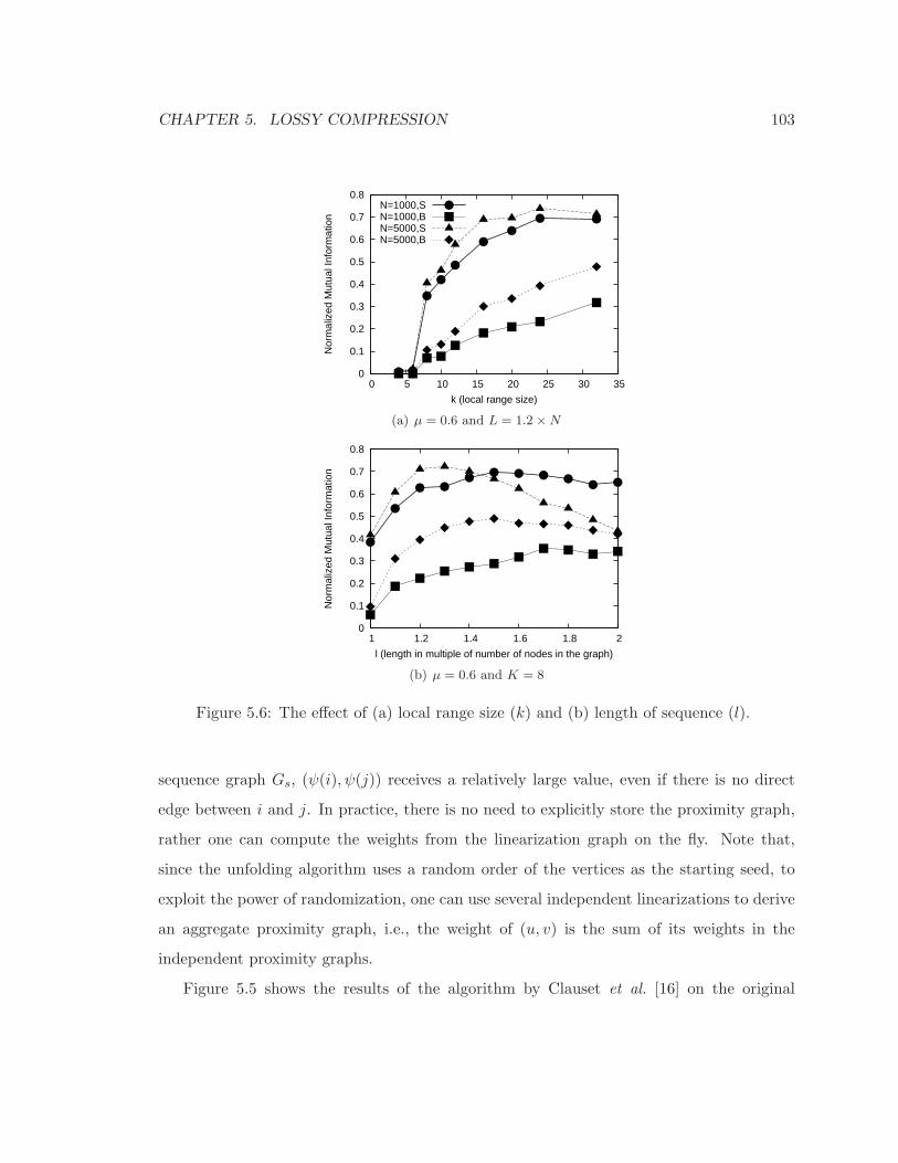
CHAPTER 5. LOSSY COMPRESSION 103
0
0.1
0.2
0.3
0.4
0.5
0.6
0.7
0.8
0 5 10 15 20 25 30 35
Nor
mal
ized
Mut
ual I
nfor
mat
ion
k (local range size)
N=1000,SN=1000,BN=5000,SN=5000,B
(a) µ = 0.6 and L = 1.2×N
0
0.1
0.2
0.3
0.4
0.5
0.6
0.7
0.8
1 1.2 1.4 1.6 1.8 2
Nor
mal
ized
Mut
ual I
nfor
mat
ion
l (length in multiple of number of nodes in the graph)
(b) µ = 0.6 and K = 8
Figure 5.6: The effect of (a) local range size (k) and (b) length of sequence (l).
sequence graph Gs, (ψ(i), ψ(j)) receives a relatively large value, even if there is no direct
edge between i and j. In practice, there is no need to explicitly store the proximity graph,
rather one can compute the weights from the linearization graph on the fly. Note that,
since the unfolding algorithm uses a random order of the vertices as the starting seed, to
exploit the power of randomization, one can use several independent linearizations to derive
an aggregate proximity graph, i.e., the weight of (u, v) is the sum of its weights in the
independent proximity graphs.
Figure 5.5 shows the results of the algorithm by Clauset et al. [16] on the original
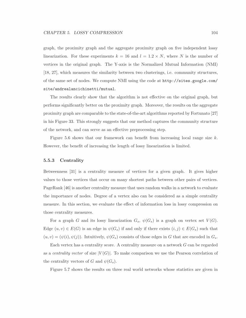
CHAPTER 5. LOSSY COMPRESSION 104
graph, the proximity graph and the aggregate proximity graph on five independent lossy
linearization. For these experiments k = 16 and l = 1.2 × N , where N is the number of
vertices in the original graph. The Y-axis is the Normalized Mutual Information (NMI)
[18, 27], which measures the similarity between two clusterings, i.e. community structures,
of the same set of nodes. We compute NMI using the code at http://sites.google.com/
site/andrealancichinetti/mutual.
The results clearly show that the algorithm is not effective on the original graph, but
performs significantly better on the proximity graph. Moreover, the results on the aggregate
proximity graph are comparable to the state-of-the-art algorithms reported by Fortunato [27]
in his Figure 33. This strongly suggests that our method captures the community structure
of the network, and can serve as an effective preprocessing step.
Figure 5.6 shows that our framework can benefit from increasing local range size k.
However, the benefit of increasing the length of lossy linearization is limited.
5.5.3 Centrality
Betweenness [31] is a centrality measure of vertices for a given graph. It gives higher
values to those vertices that occur on many shortest paths between other pairs of vertices.
PageRank [46] is another centrality measure that uses random walks in a network to evaluate
the importance of nodes. Degree of a vertex also can be considered as a simple centrality
measure. In this section, we evaluate the effect of information loss in lossy compression on
those centrality measures.
For a graph G and its lossy linearization Gs, ψ(Gs) is a graph on vertex set V (G).
Edge (u, v) ∈ E(G) is an edge in ψ(Gs) if and only if there exists (i, j) ∈ E(Gs) such that
(u, v) = (ψ(i), ψ(j)). Intuitively, ψ(Gs) consists of those edges in G that are encoded in Gs.
Each vertex has a centrality score. A centrality measure on a network G can be regarded
as a centrality vector of size |V (G)|. To make comparison we use the Pearson correlation of
the centrality vectors of G and ψ(Gs).
Figure 5.7 shows the results on three real world networks whose statistics are given in
CHAPTER 5. LOSSY COMPRESSION 105
0.3
0.4
0.5
0.6
0.7
0.8
0.9
1
0 5 10 15 20 25 30 35
Pea
rson
Cor
rela
tion
k (local range size)
PageRankBetweenness
Degree
(a) Collaboration network
0.1
0.2
0.3
0.4
0.5
0.6
0.7
0.8
0.9
1
0 5 10 15 20 25 30 35
Pea
rson
Cor
rela
tion
k (local range size)
PageRankBetweenness
Degree
(b) Wiki vote network
0.2
0.3
0.4
0.5
0.6
0.7
0.8
0.9
1
0 5 10 15 20 25 30 35
Pea
rson
Cor
rela
tion
k (local range size)
PageRankBetweenness
Degree
(c) Email exchange network
Figure 5.7: Pearson Correlation of centrality measures on original and the compressedversion
Table 5.2. As the value of k increases the correlation between the two centrality vectors
increases.
5.5.4 Running Time Efficiency
The running time of our method depends on the number of iterations in Algorithm 7. For
our setting the number of iterations is typically between 15 to 30. Figure 5.8 depicts the
running time of our method with respect to the graph size on the same LFR benchmarks
[27]. The running time of a single iteration, when parameter k is fixed, is scaling almost
linearly.
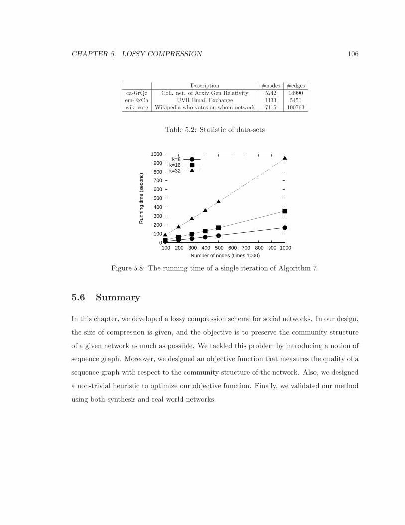
CHAPTER 5. LOSSY COMPRESSION 106
Description #nodes #edges
ca-GrQc Coll. net. of Arxiv Gen Relativity 5242 14990em-ExCh UVR Email Exchange 1133 5451wiki-vote Wikipedia who-votes-on-whom network 7115 100763
Table 5.2: Statistic of data-sets
0
100
200
300
400
500
600
700
800
900
1000
100 200 300 400 500 600 700 800 900 1000
Run
ning
tim
e (s
econ
d)
Number of nodes (times 1000)
k=8k=16k=32
Figure 5.8: The running time of a single iteration of Algorithm 7.
5.6 Summary
In this chapter, we developed a lossy compression scheme for social networks. In our design,
the size of compression is given, and the objective is to preserve the community structure
of a given network as much as possible. We tackled this problem by introducing a notion of
sequence graph. Moreover, we designed an objective function that measures the quality of a
sequence graph with respect to the community structure of the network. Also, we designed
a non-trivial heuristic to optimize our objective function. Finally, we validated our method
using both synthesis and real world networks.

CHAPTER 5. LOSSY COMPRESSION 107
Algorithm 8 Reallocation Procedure
Input: G: original graph, SeqG: sequence graph, u ∈ V (G), α: weighting parameterOutput: IPos: potential position to insert a new copy of u, Nbh: the edges associated to
the new copy of u1: C1 = ψ−1(u); C2 = ∅;2: for all {v|(u, v) ∈ E(G \ SeqG)} do3: Let p be a random member of ψ−1(v);4: C2 = C2 ∪ {p};5: N(p) = {+1}; /* neighbors of p in SeqG */6: U(p) = α; /* utility of p */7: SeqG.Insert(u, p);8: end for9: for all p ∈ C1 do
10: N(p) = SeqG.Nbh(p); U(p) =∑
a∈N(p) α|a|;
11: end for12: C = C1 ∪ C2;13: repeat14: for all {v|(u, v) ∈ E(G)} do15: Let pu and pv be s.t. (ψ(p1), ψ(p2)) = (u, v);16: /* pu ∈ C and pv ∈ ψ−1(v) */17: a = Dist(pu, pv); /* the distance in SeqG */18: U(pu) = U(pu)− α|a|;19: Let p∗u ∈ C and p∗v ∈ ψ−1(v) be s.t. maximize:
(α|dist(p∗u,p∗
v)| + U(p∗u))2 − U(p∗u)
2
20: U(p∗u) = U(p∗u) + αdist(p∗u,p∗
v);21: if p∗u 6= pu then22: N(p∗u) = N(p∗u) + {dist(p∗u, p∗v)};23: N(pu) = N(pu)− {dist(pu, pv)};24: end if25: end for26: until Convergence27: for all p ∈ C1 do28: SeqG.UpdateNeighbor(p,N(p));29: end for30: for all p ∈ C2 do31: SeqG.Delete(p);32: end for33: Let p ∈ C2 s.t. U(p) is maximum;34: IPos = p; Nbh = N(p));35: return (IPos,Nbh);
Chapter 6
Conclusion
The central idea of the thesis is to use a notion of “linearization of the nodes” in order to
design a General Purpose Social Network (GPSN) compression framework. The study has
three main components: the Eulerian data structure, the lossless GPSN compression scheme
and the lossy GPSN compression scheme. All three components are different settings of the
same framework. The Eulerian data structure is the simplest setting for which we can have
an analytical analysis. The lossless compression scheme, comparing to the Eulerian data
structure, is a more general setting of the framework, where the goal is to represent all the
edges of the network using the least number of bits. However, for the lossy compression
scheme, we assume that there is a constraint on the available storage, and the goal is to
encode as much as “information” as possible.
6.1 Summary
We like to highlight the following main contributions of this dissertation:
• The Eulerian Data Structure. The novel Eulerian data structure is a non-trivial
data structure which is memory efficient for any type of network, including real world
social networks. To the best of our knowledge, this is the first data structure for
network data that allows both efficient in-neighbor and out-neighbor queries without
108
CHAPTER 6. CONCLUSION 109
replicating the data.
A solid process for evaluating a computational system is to provide a proof for efficiency
and correctness of the system. The Eulerian data structure is a setting of the GPSN
compression framework for which it is possible to prove an upper bound on the bits-
per-edge rate. To the best of our knowledge this is the only nontrivial upper bound on
the bits-per-edge rate of any representation scheme for social networks. We compare
the upper bound with the trivial baseline data structure that can answer both in-
neighbor and out-neighbor queries, which is the adjacency list representation of the
network and the transpose of it. Chapter 3 provides an in-depth discussion on the
Eulerian data structure.
• Lossless Compression Scheme. We exploit the notions of k-linearization, and
multi-level linearization introduced in Section 3.2.4, in order to design a general pur-
pose lossless compression scheme. Interestingly, this approach reduces the social net-
work compression to a combinatorial optimization problem. However, we believe find-
ing the optimal solution of this problem is NP-hard. We develop a heuristic algorithm
to construct the compressed network. A comprehensive set of experiments has been
conducted to study the compression rate of the lossless compression scheme. Chapter
4 presents the experimental study for the lossless GPSN compression scheme.
The lossless compression scheme is a practical setting of the GPSN framework, and
there is no upper bound on its compression rate. However, experimentally, we compare
the bits-per-edge rate of lossless compression scheme with the results reported in [14]
for those publicly available datasets. Note that the framework used in this study
does not support sub-linear incremental updates, nor efficient in-neighbor queries.
Therefore, to justify our lossless compression scheme, we do not require a significant
improvement of the compression rate, rather we show that the compression rate is
comparable.
CHAPTER 6. CONCLUSION 110
• Lossy Compression Scheme. The challenge of developing a lossy network com-
pression framework has two folds. First, it is the matter of designing an efficient rep-
resentation scheme to represent the links, and second, having a mechanism in place to
determine whether a given edge, or vertex, has to be included in the compression. For
this part of the thesis, we show that the GPSN compression framework, in addition to
being storage-efficient, offers a natural edge ranking mechanism. Chapter 5 discusses
the lossy compression scheme in details.
For the lossy compression, the goal is to encode as much as possible information
using a given amount of memory. Therefore, the compression rate does not have a
straightforward meaning here. However, a notion of utility can be useful. Bit-utility-
rate measures the amount of information that a single bit represents, that is the
number of edges over the number of bits. For example, the meaning of a bit-utility-
rate of 0.5 is that for representing a certain number of edges, the lossy scheme uses
twice as many bits. We evaluate the bit-utility-rate of our lossy compression scheme.
One might argue that the edges in a real world social network are not of the same
importance. The majority of them form a community structure for the network, while
others considered being abnormal or even depending on the context, regarded as noise.
From this perspective, a legitimate question is that what would the lossy compression
scheme do to the community structure of the network. A set of experiments introduced
in Section 5.5 evaluate the effect of lossy compression on the community structure of
the network. We show that our framework is quit effective in capturing the global
community structure of a given social network.
6.2 Future Work
There are several future directions for this dissertation, both from theoretical and practical
perspectives. We distinguish five interesting directions for further investigation:
CHAPTER 6. CONCLUSION 111
• Hardness Result. From a theoretical point of view, a hardness result for the problem
of finding the optimal k-linearization, when k is fixed, would be interesting.
• Approximation Algorithm. Assuming the problem is NP-hard, the next natu-
ral question would concern the existence of a nontrivial approximation algorithm for
finding the optimal k-linearization. The optimal 1-linearization is already a k approx-
imation for the problem, and since finding the optimal 1-linearization can be done
in linear time, therefore we have a k-approximation algorithm. Then, the accurate
question is that can we have an approximation algorithm with a factor better than k?
• Upper Bound. Having an upper bound on the length of the optimal k-linearization
would give us an upper bound on the compression rate. Proving an upper bound for
general graphs might be hard. However, having some assumption on the structure of
the network could make the problem easier. For example, proving an upper bound
parametrized by the number of edges and the Global Clustering Coefficient might not
be out of reach.
• Better Linearization. As for the practical side, exploring alternative methods for
linearizing a given network, is of great interest. We believe the study of this disser-
tation should be regarded as a baseline both for lossless and lossy compression. As a
possible future direction, developing linearization methods based on spectral analysis
of the network could be quit fruitful both for lossless and lossy compression.
• Distributed Computing. Another interesting direction for exploring further is the
possibility of extending the GPSN framework to a distributed network management
system. We believe the notion of linearization suggests a natural partitioning paradigm
that relies on partitioning of the edges rather than the nodes of a given network.

Bibliography
[1] G. Ausiello, M. Protasi, A. Marchetti-Spaccamela, G. Gambosi, P. Crescenzi, and
V. Kann. Complexity and Approximation: Combinatorial Optimization Problems and
Their Approximability Properties. Springer-Verlag New York, Inc., Secaucus, NJ, USA,
1st edition, 1999.
[2] M. J. Barber and J. W. Clark. Detecting network communities by propagating labels
under constraints. Physical Review E, 80(2):026129+, Aug. 2009.
[3] T. Berners-Lee and M. Fischetti. Weaving the web: The original design and ultimate
destiny of the world wide web by its inventor. Harper, San Francisco, 1999.
[4] K. Bharat, A. Broder, M. Henzinger, P. Kumar, and S. Venkatasubrama-
nian. The connectivity server: fast access to linkage information on the
web. In 7th International WWW Conference, Brisbane, Australia, 1998.
http://www7.scu.edu.au/programme/fullpapers/1938/com1938.htm.
[5] A. Blum, G. Konjevod, R. Ravi, and S. Vempala. Semi-definite relaxations for minimum
bandwidth and other vertex-ordering problems. In J. S. Vitter, editor, STOC, pages
100–105. ACM, 1998.
[6] P. Boldi, M. Rosa, M. Santini, and S. Vigna. Layered label propagation: a multireso-
lution coordinate-free ordering for compressing social networks. In Proceedings of the
20th international conference on World wide web, WWW ’11, pages 587–596, New
York, NY, USA, 2011. ACM.
112
BIBLIOGRAPHY 113
[7] P. Boldi, M. Santini, and S. Vigna. Permuting web graphs. In Proceedings of the
6th International Workshop on Algorithms and Models for the Web-Graph (WAW’09),
pages 116–126, Berlin, Heidelberg, 2009. Springer-Verlag.
[8] P. Boldi and S. Vigna. The webgraph framework I: compression techniques. In WWW,
pages 595–602, 2004.
[9] P. Boldi and S. Vigna. The webgraph framework II: Codes for the world-wide web. In
Data Compression Conference, page 528, 2004.
[10] A. Z. Broder, M. Charikar, A. M. Frieze, and M. Mitzenmacher. Min-wise independent
permutations. J. Comput. Syst. Sci., 60(3):630–659, 2000.
[11] G. Buehrer and K. Chellapilla. A scalable pattern mining approach to web graph
compression with communities. In WSDM, pages 95–106, 2008.
[12] G. Buehrer, K. Chellapilla, and S. Parthasarathy. Itemset mining in log-linear time. In
OSU-CISRC-11/07-TR76, 2007.
[13] T. F. Chan, J. Cong, T. Kong, J. R. Shinnerl, and K. Sze. An enhanced multilevel
algorithm for circuit placement. In Proceedings of the 2003 IEEE/ACM international
conference on Computer-aided design, ICCAD ’03, pages 299–, Washington, DC, USA,
2003. IEEE Computer Society.
[14] F. Chierichetti, R. Kumar, S. Lattanzi, M. Mitzenmacher, A. Panconesi, and P. Ragha-
van. On compressing social networks. In KDD, pages 219–228, 2009.
[15] F. R. K. Chung. Spectral Graph Theory.
[16] A. Clauset, M. E. J. Newman, , and C. Moore. Finding community structure in very
large networks. Physical Review E, pages 1– 6, 2004.
[17] T. Cour, F. Bnzit, and J. Shi. Spectral segmentation with multiscale graph decompo-
sition. In CVPR (2), pages 1124–1131. IEEE Computer Society, 2005.
BIBLIOGRAPHY 114
[18] L. Danon, J. Duch, A. Diaz-Guilera, and A. Arenas. Comparing community structure
identification, Oct. 2005.
[19] J. Dıaz, J. Petit, and M. J. Serna. A survey of graph layout problems. ACM Comput.
Surv., 34(3):313–356, 2002.
[20] C. H. Q. Ding, X. He, H. Zha, M. Gu, and H. D. Simon. A min-max cut algorithm for
graph partitioning and data clustering. In Proceedings of the 2001 IEEE International
Conference on Data Mining, ICDM ’01, pages 107–114, Washington, DC, USA, 2001.
IEEE Computer Society.
[21] D. Easley and J. Kleinberg. Networks, Crowds, and Markets: Reasoning About a Highly
Connected World. Cambridge University Press, 2010.
[22] M. Ester, H.-P. Kriegel, J. Sander, and X. Xu. A density-based algorithm for discovering
clusters in large spatial databases with noise. In KDD, pages 226–231, 1996.
[23] T. Feder and R. Motwani. Clique partitions, graph compression and speeding-up algo-
rithms. J. Comput. System Sci., 51(2):261–271, 1995. Earlier version in STOC’91.
[24] U. Feige and J. R. Lee. An improved approximation ratio for the minimum linear
arrangement problem. Inf. Process. Lett., 101(1):26–29, 2007.
[25] M. R. Fellows and M. A. Langston. On search, decision, and the efficiency of
polynomial-time algorithms. J. Comput. Syst. Sci., 49(3):769–779, 1994.
[26] G. W. Flake, S. Lawrence, and C. L. Giles. Efficient identification of web communi-
ties. In Proceedings of the sixth ACM SIGKDD international conference on Knowledge
discovery and data mining, KDD ’00, pages 150–160, New York, NY, USA, 2000. ACM.
[27] S. Fortunato. Community detection in graphs. Physics Reports, 486(3-5):75 – 174,
2010.
BIBLIOGRAPHY 115
[28] J. Gao, W. Yuan, X. Li, K. Deng, and J.-Y. Nie. Smoothing clickthrough data for web
search ranking. In J. Allan, J. A. Aslam, M. Sanderson, C. Zhai, and J. Zobel, editors,
SIGIR, pages 355–362. ACM, 2009.
[29] M. R. Garey and D. S. Johnson. Computers and Intractability: A Guide to the Theory
of NP-Completeness. W.H. Freeman and Co., San Francisco, CA, 1979.
[30] D. Gibson, R. Kumar, and A. Tomkins. Discovering large dense subgraphs in massive
graphs. In K. Bohm, C. S. Jensen, L. M. Haas, M. L. Kersten, P.-A. Larson, and B. C.
Ooi, editors, VLDB, pages 721–732. ACM, 2005.
[31] M. Girvan and M. E. Newman. Community structure in social and biological networks.
Proc Natl Acad Sci U S A, 99(12):7821–7826, June 2002.
[32] C. Hierholzer. ber die mglichkeit, einen linienzug ohne wiederholung und ohne unter-
brechung zu umfahren. J. Math. Ann, 6:30–32, 1873.
[33] G. Karypis and V. Kumar. Multilevel algorithms for multi-constraint graph partition-
ing. In Proceedings of the 1998 ACM/IEEE conference on Supercomputing (CDROM),
Supercomputing ’98, pages 1–13, Washington, DC, USA, 1998. IEEE Computer Soci-
ety.
[34] R. Kumar, P. Raghavan, S. Rajagopalan, and A. Tomkins. Trawling the web for
emerging cyber-communities. In Proceedings of the eighth international conference on
World Wide Web, WWW ’99, pages 1481–1493, New York, NY, USA, 1999. Elsevier
North-Holland, Inc.
[35] A. Lancichinetti, S. Fortunato, and F. Radicchi. Benchmark graphs for testing com-
munity detection algorithms. Phys. Rev. E, 78(4):046110, Oct. 2008.
[36] J. Leskovec, J. Kleinberg, and C. Faloutsos. Graphs over time: Densification laws,
shrinking diameters and possible explanations. In In KDD, pages 177–187. ACM Press,
2005.
BIBLIOGRAPHY 116
[37] J. Leskovec, K. J. Lang, A. Dasgupta, and M. W. Mahoney. Statistical properties of
community structure in large social and information networks. In WWW ’08: Pro-
ceeding of the 17th international conference on World Wide Web, pages 695–704, New
York, NY, USA, 2008. ACM.
[38] U. Luxburg. A tutorial on spectral clustering. Statistics and Computing, 17:395–416,
December 2007.
[39] J. R. Magnus. Handbook of matrices. Econometric Theory, 14(03):379–380, 1998.
[40] H. Maserrat and J. Pei. Neighbor query friendly compression of social networks. InKDD
’10: Proceedings of the 16th ACM SIGKDD international conference on Knowledge
discovery and data mining, pages 533–542, New York, NY, USA, 2010. ACM.
[41] S. Navlakha, R. Rastogi, and N. Shrivastava. Graph summarization with bounded
error. In SIGMOD Conference, pages 419–432, 2008.
[42] M. E. Newman and M. Girvan. Finding and evaluating community structure in net-
works. Phys Rev E Stat Nonlin Soft Matter Phys, 69(2):026113.1–15, Feb. 2004.
[43] M. E. J. Newman and M. Girvan. Finding and evaluating community structure in
networks. Physical Review, E 69(026113), 2004.
[44] A. Y. Ng, M. I. Jordan, and Y. Weiss. On spectral clustering: Analysis and an algo-
rithm. In Advances in Neural Information Processing Systems 14, pages 849–856. MIT
Press, 2001.
[45] L. Page, S. Brin, R. Motwani, and T. Winograd. The pagerank citation ranking:
Bringing order to the web. In Proceedings of the 7th International World Wide Web
Conference, pages 161–172, Brisbane, Australia, 1998.
[46] L. Page, S. Brin, R. Motwani, and T. Winograd. The pagerank citation ranking:
Bringing order to the web. Technical Report 1999-66, Stanford InfoLab, November
1999. Previous number = SIDL-WP-1999-0120.

BIBLIOGRAPHY 117
[47] C. H. Papadimitriou. The NP-completeness of the bandwidth minimization problem.
Computing, 16(3):263–270, 1976.
[48] J. Petit. Combining spectral sequencing and parallel simulated annealing for the minla
problem. Parallel Processing Letters, 13(1):77–91, 2003.
[49] J. Petit. Experiments on the minimum linear arrangement problem. ACM Journal of
Experimental Algorithmics, 8, 2003.
[50] S. Raghavan and H. Garcia-Molina. Representing web graphs. In ICDE, pages 405–416,
2003.
[51] U. N. Raghavan, R. Albert, and S. Kumara. Near linear time algorithm to detect
community structures in large-scale networks. PHYSICAL REVIEW E, 76:036106,
2007.
[52] K. H. Randall, R. Stata, J. L. Wiener, and R. Wickremesinghe. The link database:
Fast access to graphs of the web. In DCC, pages 122–131, 2002.
[53] E. Rodriguez-Tello, J.-K. Hao, and J. Torres-Jimenez. Memetic algorithms for the
minla problem. In E.-G. Talbi, P. Liardet, P. Collet, E. Lutton, and M. Schoenauer,
editors, Artificial Evolution, volume 3871 of Lecture Notes in Computer Science, pages
73–84. Springer, 2005.
[54] P. Ronhovde and Z. Nussinov. Multiresolution community detection for megascale
networks by information-based replica correlations. Phys. Rev. E, 80(1):016109, Jul
2009.
[55] P. Ronhovde and Z. Nussinov. Local resolution-limit-free potts model for community
detection. Physical Review E, 81(4):046114+, Apr. 2010.
[56] P. Ronhovde and Z. Nussinov. Local resolution-limit-free potts model for community
detection. PHYSICAL REVIEW E, 81:046114, 2010.
BIBLIOGRAPHY 118
[57] I. Safro, D. Ron, and A. Brandt. Multilevel algorithms for linear ordering problems. J.
Exp. Algorithmics, 13:4:1.4–4:1.20, February 2009.
[58] K. Stuben. A review of algebraic multigrid. J. Comput. Appl. Math., 128:281–309,
March 2001.
[59] V. V. Vazirani. Approximation algorithms. Springer-Verlag New York, Inc., New York,
NY, USA, 2001.
[60] D. Wagner and F. Wagner. Between min cut and graph bisection. In Proceedings of
the 18th International Symposium on Mathematical Foundations of Computer Science,
MFCS ’93, pages 744–750, London, UK, UK, 1993. Springer-Verlag.
[61] N. Wang, S. Parthasarathy, K.-L. Tan, and A. K. H. Tung. Csv: visualizing and
mining cohesive subgraphs. In Proceedings of the 2008 ACM SIGMOD international
conference on Management of data, SIGMOD ’08, pages 445–458, New York, NY, USA,
2008. ACM.
[62] D. J. Watts and S. H. Strogatz. Collective dynamics of small-world networks. Nature,
393(6684):440–442, June 1998.
[63] X. Xu, N. Yuruk, Z. Feng, and T. A. J. Schweiger. Scan: a structural clustering
algorithm for networks. In KDD, pages 824–833, 2007.
[64] S. X. Yu and J. Shi. Multiclass spectral clustering. In ICCV, pages 313–319. IEEE
Computer Society, 2003.
[65] L. Zelnik-Manor and P. Perona. Self-tuning spectral clustering. In NIPS, 2004.