Compressed Sensing Petrov-Galerkin

Approximations for Parametric PDEs

J.-L. Bouchot and B. Bykowski and H. Rauhut and Ch. Schwab

Research Report No. 2015-09February 2015

Seminar für Angewandte MathematikEidgenössische Technische Hochschule

CH-8092 ZürichSwitzerland

____________________________________________________________________________________________________

Compressed Sensing Petrov-Galerkin

Approximations for Parametric PDEs

Jean-Luc Bouchot, Benjamin Bykowski, and Holger Rauhut

Chair for Mathematics C (Analysis)

RWTH Aachen University

Email: {bouchot,rauhut}@mathc.rwth-aachen.de

benjamin.bykowski@rwth-aachen.de

Christoph Schwab

Seminar of Applied Mathematics

ETH Zurich

Email: christoph.schwab@sam.math.ethz.ch

Abstract—We consider the computation of parametric solutionfamilies of high-dimensional stochastic and parametric PDEs.We review recent theoretical results on sparsity of polynomialchaos expansions of parametric solutions, and on compressedsensing based collocation methods for their efficient numericalcomputation.

With high probability, these randomized approximations real-ize best N -term approximation rates afforded by solution sparsityand are free from the curse of dimensionality, both in terms ofaccuracy and number of samples evaluations (i.e. PDE solves).

Through various examples we illustrate the performance ofCompressed Sensing Petrov-Galerkin (CSPG) approximations ofparametric PDEs, for the computation of (functionals of) solu-tions of intregral and differential operators on high-dimensionalparameter spaces. The CSPG approximations allow to reduce thenumber of PDE solves, as compared to Monte-Carlo methods,while being likewise nonintrusive, and being “embarassinglyparallel”, unlike dimension-adaptive collocation or Galerkinmethods.

I. INTRODUCTION

A. Problem statement

We consider the problem of computing an (accurate) ap-

proximation of a parametric family u defined on a bounded,

“physical” domain D ⊂ Rd and depending on possibly

countably many parameters y = (yj)j≥1 ∈ U = [−1, 1]Nimplicitly through the parametric operator equation

A(y)u(y) = f. (1)

Equation (1) is assumed to be well-posed in a reflexive,

separable Banach space V , uniformly for all parameter se-

quences y ∈ U . From a Bochner space perspective, if the

parameters y are distributed according to a certain distribution

µ on U , we are looking for strongly µ-measurable maps

u ∈ L(U, V ;µ). For simplicity of exposition, we assume here

as in [1], [2] that A(y) in (1) can be expressed as a linear

combination of bounded linear operators (Aj)j≥0 : V →W ′,where W is a suitable second (separable and reflexive) Banach

space, such that A(y) = A0 +∑

j≥1 yjAj in L(V,W ′). We

hasten to add that the principal conclusions of the present

work apply to larger classes of countably-parametric operator

equations (1) with sparse solution families. Given a parametric

family f(y) ∈ W ′, we wish to approximate numerically the

corresponding parametric solution family {u(y) : y ∈ U}. To

simplify the exposition, we restrict ourselves in this note to

nonparametric data f ; all results which follow apply verbatim

in the general case. We consider the case which appears often

in practice, of approximation of functionals of the parametric

solution: given G ∈ L(V,R), approximate numerically the map

F : U → R, F (y) := G(u(y)).

B. Tools and ideas

The present CSPG approach is motivated by recent sparsity

results for the parametric solution maps in [3], [4] where spar-

sity results for coefficient sequences of generalized polynomial

chaos (GPC) expansions of u(y) were established. The term

GPC expansion refers to u(y) =∑

j∈F xjϕj(y) for some

basis (ϕj)j∈F of L2µ(U), indexed on the countable family F .

Due to the boundedness and linearity of G, we can similarly

write F (y) =∑

j∈F gjϕj . Knowing the compressibility of the

coefficient sequence (gj)j≥0 (i.e., there exists 0 < p < 1, such

that ‖g‖p <∞), the computational challenge is to recover only

the most important ones using only as few as possible solves

of (1), while ensuring a given accuracy. The sparsity of the

GPC coefficient sequence together with Stechkin inequality

ensures that σs(g)q ≤ s1/q−1/p‖g‖p,0 < p < q, where σs(g)qdenotes the best s-term approximation of g in the q norm.

In other words, the coefficient sequence g can be compressed

with high accuracy and hence (see Theorem 1 in Section II-B)

the function F can be well approximated. To overcome the

curse of dimensionality incurred by CS based methods (see [2,

Eq.(1.16)]), we propose an extension based on ℓp,ω spaces [5].

The rest of the paper is organized as follows. Section II

reviews the mandatory background on weighted compressed

sensing, Petrov-Galerkin approximations, and their combined

use for high-dimensional PDEs. Section III then introduces

various model problems to numerically validate the theoretical

results. We provide numerical experiments which show that

the CSPG method can be easily implemented for various

linear functionals G, even with a large number of parameters.

For the parametric model diffusion problems, we compare

the convergence of the expectation with that of Monte-Carlo

methods.

II. REVIEW ON COMPRESSED SENSING

PETROV-GALERKIN APPROXIMATIONS

A. Generalized Polynomial Chaos (GPC) expansions and ten-

sorized Chebyshev polynomials

GPC expansion of the parametric solution family {u(y) :y ∈ U} of Eq. (1) are orthogonal expansions of u(y) in

terms of tensorized Chebyshev polynomials (Tν)ν∈F , here Fdenotes the countable set of multiindices with finite support

(F := {ν ∈ NN0 : | supp(ν)| <∞}):

u(y) =∑

ν∈FdνTν(y). (2)

Note that here the coefficients dν are functions in V and that

the expansion is in terms of the parameter sequences y ∈ Uand not in the spatial coordinates. The tensorized Chebyshev

polynomials are defined as Tν(y) =∏∞

j=1 Tνj (yj), y ∈ U ,

with Tj(t) =√2 cos (j arccos(t)) and T0(t) ≡ 1.

Defining σ the probability measure on [−1; 1] as dσ(t) :=dt

π√1−t2

, Chebyshev polynomials form an orthonormal system

in the sense that∫ 1

−1 Tk(t)Tl(t)dσ(t) = δk,l for k, l ∈ N0.

Similarly, with the product measure dη(y) :=⊗

j≥1 dσ(yj),the tensorized Chebyshev polynomials are orthonormal in the

sense that∫

y∈U

Tµ(y)Tν(y)dη(y) = δµ,ν , for µ, ν ∈ F .

An important result proven in [6] ensures the ℓp summabil-

ity, for some 0 < p ≤ 1, of the Chebyshev polynomial chaos

expansion (2) of the solution of the model affine-parametric

diffusion equation

−∇ · (a∇u) = f , (3)

where a admits the affine-parametric expansion

a(y;x) = a0(x) +∑

j≥1

yjaj(x) . (4)

Specifically,∥∥(‖dν‖V )ν∈F

∥∥pp=

∑ν∈F ‖dν‖

pV < ∞under

the condition that the sequence of inifinity norms of the aj is

itself ℓp summable:

∥∥∥(‖aj‖∞)j≥1

∥∥∥p<∞.

These results were extended to the weighted ℓp spaces

(see Section II-B) for the more general parametric operator

problem, Eq.(1) with linear parameters, in [2]: (‖dν‖V )ν∈F ∈ℓω,p(F) under certain assumptions, and with Eq. (6) defining

the weighted ℓp spaces.

B. Weighted compressed sensing

The last decade has seen the emergence of compressed sens-

ing [7] as a method to solve underdetermined linear systems

Ax = y under sparsity constraints ‖x‖0 := | supp(x)| ≤ s.

Some work has focused on finding conditions on A such that

the problem

x# = argmin ‖x‖1, s.t. ‖Ax− y‖2 ≤ η (5)

yields an exact and unique solution. One known condition is

that the matrix A should fulfill a Restricted Isometry Property

(RIP) of order s and constant δ for reasonable values of s and

δ. A is said to have RIP(s, δ) if, for any s- sparse vector x,

|‖Ax‖22 − ‖x‖22| ≤ δ‖x‖22. In other words, for small δ, the

matrix A behaves almost like an isometry on sparse vectors.

In parallel, the community also focused on finding matrices

obeying the RIPs. While the problem of finding deterministic

matrices with interesting RIPs is still open, it has been proven

that random matrices are good candidates [8].

More recently, results from compressed sensing have been

generalized to handle weighted sparsity [5]. In a similar man-

ner, given a weight sequence (ωj)j∈Λ, ωj ≥ 1, one can derive

weighted sparsity of a vector x as ‖x‖ω,0 :=∑

j∈supp(x) ω2j .

Similarly, weighted ℓp norms are defined, for 0 < p ≤ 2 as

‖x‖ω,p =(∑

j∈Λ ω2−pj |xj |p

)1/p

and the associated spaces

are defined as

ℓp,ω(Λ) := {x ∈ RΛ : ‖x‖p,ω <∞} . (6)

Weigthed ℓp can be further extended to functions f =∑j≥1 xjϕj expanded in certain basis elements (ϕj)j≥1 as

|||f |||ω,p := ‖x‖ω,p. This in particular is interesting for function

interpolation from very few samples:

Theorem 1 (Complete statement in [5]). For (ϕj)j∈Λ a

countable orthonormal system and a sequence of weights

ωj ≥ ‖ϕj‖∞, there exists a finite subset Λ0 with N = |Λ0|such that drawing m ≥ c0s log

3(s) log(N) samples at random

ensures that, with high probability,

‖f − f#‖∞ ≤∣∣∣∣∣∣f − f#

∣∣∣∣∣∣ω,1≤ c1σs(f)ω,1, (7)

‖f − f#‖2 ≤ d1σs(f)ω,1/√s (8)

where f :=∑

j∈Λ xjϕj is the function to recover, and

f#(y) :=∑

j∈Λ0x#j ϕj(y) is the solution obtained via

weighted ℓ1 minimization.

In particular, the previous theorem offers error bounds in

both L2 and L∞ norms.

C. Petrov-Galerkin Approximations

Petrov-Galerkin (PG) approximations of a function u ∈ Vdefined on D are based on one-parameter families of nested

and finite-dimensional subspaces {V h}h and {Wh}h which

are dense in V and W , respectively (with the discretization

parameter h denoting e.g. meshwidth of triangulations in Finite

Element methods, or the reciprocal of the spectral order in

spectral methods). Given y ∈ U , the PG projection of u(y)onto V h, uh(y) := Gh(u(y)), is defined as the unique solution

of the finite-dimensional, parametric variational problem: Find

uh ∈ V h such that

(A(y)uh(y))(wh) = f(wh), ∀wh ∈ Wh . (9)

Note that for A(y) boundedly invertible and under some

(uniform w.r. to y ∈ U and w.r. to h) inf-sup conditions

(see, e.g. [1, Prop. 4]) the PG projections Gh in (9) are well-

defined and quasioptimal uniformly w.r. to y ∈ U : there exists

a constant C > 0 such that for all y ∈ U csand h > 0sufficiently small it holds

‖u(y)− uh(y)‖V ≤ C infvh∈V h ‖u(y)− vh‖V . (10)

D. Review of the CSPG algorithm

We review the CSPG algorithm of [2]. It relies on the

evaluation of m solutions b(l) := G(u(y(l))) of Eq. (1) given

m randomly chosen parameter instances y(l) = (y(l)j )j≥1,

1 ≤ l ≤ m. These real-valued solutions b(l) are then

used in a weighted ℓ1 minimization program in order to

determine the most significant coefficients in expansion (2),

see Algorithm 11.

Data: Weights (vj)j≥1, an accuracy ε and sparsity sparameters, a multiindex set J s

0 with

N = |J s0 | <∞, a compressibility parameter

0 < p < 1, and a number of samples m.

Result:(g#ν

)ν∈J s

0

, a CS-based approximation of the

coefficients (gν)ν∈J s0

.

for l = 1, · · · ,m do

Draw y(l) at random;

Numerically estimate b(l);end

(Φ)l,ν ← Tν(y(l)), ν ∈ J s

0 , 1 ≤ l ≤ m

ων ← 2‖ν‖0/2∏

j:νj 6=0

vνjj , ν ∈ J s

0 (11)

Compute g# as the solution of

min ‖g‖ω,p, s.t. ‖Φg − b‖2 ≤ 2√mε (12)

Algorithm 1: Pseudo-code for the CSPG Algorithm

Before we justify the use of this algorithm, it is worth

mentioning the roles of the different parameters: ε is an accu-

racy parameter that will have an impact on the discretization

parameter h and on the number of samples required. The

importance and impact of the choice of the weight sequence

(vj)j≥1 is still not clear and is left for future research. The

index set J s0 ⊂ F (see definition below) acts as an estimation

of the optimal set containing the best s-(weighted) sparse

approximation of F .

Theorem 2 ([2]). Let u(y) be the solution to Eq. (1) such that

A0 is boundedly invertible and∑

j≥1 β0,j ≤ κ ∈ (0, 1) where

β0,j := ‖A−10 Aj‖L(V,V ), and the scales of smoothness spaces

have a parametric regularity property (see [2, Assumption

2.3]). If the sequence (vj)j≥1 is such that∑

j β0,jv(2−p)/pj ≤

κv,p ∈ (0, 1) and (β0,j)j ∈ ℓv,p then g ∈ ℓω,p with ω as in

Eq. (11). Define an accuracy ε > 0 and sparsity s such that√5 41−1/ps1/2−1/p‖g‖ω,p ≤ ε ≤ C2s

1/2−1/p‖g‖ω,p, (13)

with C2 >√541−1/p independent of s and define J s

0 := {ν ∈F : 2‖ν‖0

∏j:νj 6=0 v

2νjj ≤ s/2} with N := |J s

0 |. Pick m ≍Cs log3(s) log(N) (C a universal constant) samples i.i.d at

random w.r.t. to the Chebyshev distribution and define F (y) :=

1Due to space constraints some details are omitted. We refer to [2] fordetails.

∑ν∈J s

0

g#ν (y) with g# solution of Eq. (12). Then, there exists

a (universal) constant C′ such that, with probability at least

1− 2N− log3(s), it holds:

‖F − F‖2 ≤ C′‖g‖ω,ps1/2−1/p ≤ C′′

g

(log3(m) log(N)

m

)1/p−1/2

,

(14)

‖F − F‖∞ ≤ C′‖g‖ω,ps1−1/p ≤ C′′

g

(log3(m) log(N)

m

)1/p−1

,

(15)

where C′′g depends on C′ and ‖g‖ω,p.

III. NUMERICAL EXAMPLES

For the empirical validation of the theories introduced

in the previous sections, we consider various use cases in

1-dimensional physical domains. We are mostly interested

in the high-dimensionality of the parameter space U . The

physical domain of the operator equation (1) renders the PG

discretization more complicated but does not affect the CS

access to the parameter space U .

In the numerical examples we consider model affine-

parametric diffusion equations (3), (4). As stated in the in-

troduction, we consider y = (yj)j≥1 ∈ U and x ∈ D = [0, 1].For the practical numerical results, we use trigonometric

polynomials as basis functions aj in (4), for a constant α:

a2j−1(x) =cos(jπx)

jα, a2j(x) =

sin(jπx)

jα. (16)

We used the nominal field a0 = 0.1 + 2ζ(α, 1) where

ζ(α, 1) :=∑

n≥11nα .The remaining parameters are set as:

• f ≡ 10,

• For j ≥ 1, vj = γjτ , where γ = 1.015 and τ =log(⌊√s/2γ⌋)/ log(d), then v2j−1 = v2j = vj , j ≥ 1,2

• α = 2, ε = 0.5 · 10−9,

• m = 2s log(s) log(N)3 with J s0 denoting the initial set

of important coefficients of the GPC, and N := |J s0 |. s

varies from 30 to 500, see Table I for examples.4

Note that no values are assigned for the compressibility

parameter p. While it is of prime importance in the theoretical

analysis and for the understanding of the algorithm, it has no

effect on the implementation. For information purposes, we

have also given the bounds on the error in Table I for a com-

pressibility parameter p = 1/2 (i.e. err1/p−1/2 and err1/p−1,

resp. for the L2 and L∞ norms, where err = log3(m) log(N)m ).

Be aware that these estimations do not include the constant

C′′g in front in Eqs. (14) and (15). Another remark regarding

the implementation is that the number of variables has been

trunctaed to d = 20 parameters (i.e. k stops at 10 in the

expansion of the diffusion coefficient).

2doubling the vj ensures that the sin and cos functions with the samefrequencies are given the same weights.

3This number of samples is different than the one suggested in the theorem.This is motivated by results on nonuniform recovery from random matricesin compressed sensing - see [7, Ch.9.2].

4The size of the initial set depends on the sparsity and on the weights. Thenumbers given here are only valid for the setting described above.

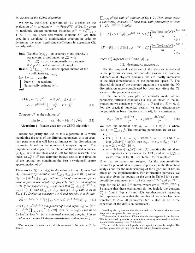
(a) Expectation in the L2 norm of the MC esti-mation (blue) and CSPG (green) methods.

(b) Estimation of the convergence of the L2 errornorm for CSPG.

(c) Estimation of the convergence of the L∞ errornorm for CSPG.

Fig. 1. Numerical results of the average of the solution of the operator equation (1) (see text for details).

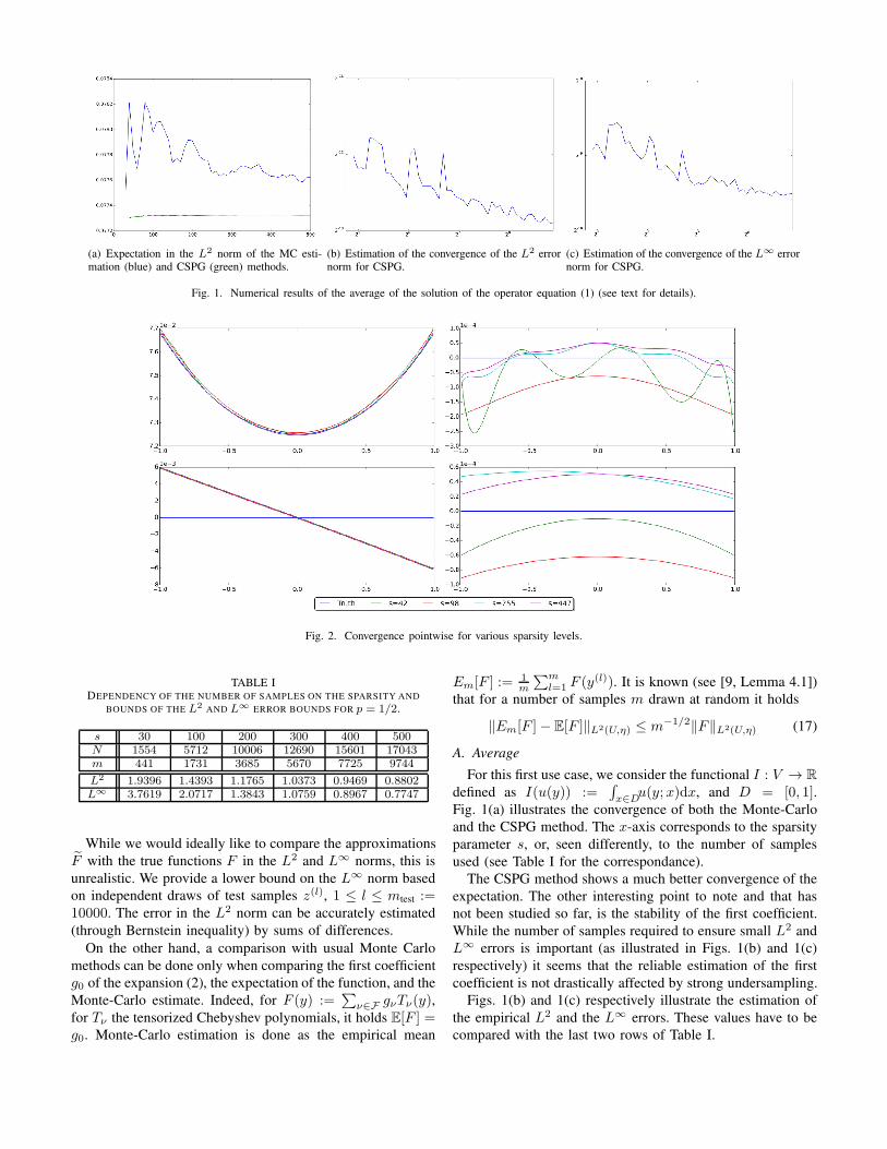
Fig. 2. Convergence pointwise for various sparsity levels.

TABLE IDEPENDENCY OF THE NUMBER OF SAMPLES ON THE SPARSITY AND

BOUNDS OF THE L2 AND L∞ ERROR BOUNDS FOR p = 1/2.

s 30 100 200 300 400 500

N 1554 5712 10006 12690 15601 17043

m 441 1731 3685 5670 7725 9744

L2 1.9396 1.4393 1.1765 1.0373 0.9469 0.8802L∞ 3.7619 2.0717 1.3843 1.0759 0.8967 0.7747

While we would ideally like to compare the approximations

F with the true functions F in the L2 and L∞ norms, this is

unrealistic. We provide a lower bound on the L∞ norm based

on independent draws of test samples z(l), 1 ≤ l ≤ mtest :=10000. The error in the L2 norm can be accurately estimated

(through Bernstein inequality) by sums of differences.

On the other hand, a comparison with usual Monte Carlo

methods can be done only when comparing the first coefficient

g0 of the expansion (2), the expectation of the function, and the

Monte-Carlo estimate. Indeed, for F (y) :=∑

ν∈F gνTν(y),for Tν the tensorized Chebyshev polynomials, it holds E[F ] =g0. Monte-Carlo estimation is done as the empirical mean

Em[F ] := 1m

∑ml=1 F (y(l)). It is known (see [9, Lemma 4.1])

that for a number of samples m drawn at random it holds

‖Em[F ]− E[F ]‖L2(U,η) ≤ m−1/2‖F‖L2(U,η) (17)

A. Average

For this first use case, we consider the functional I : V → R

defined as I(u(y)) :=∫x∈D

u(y;x)dx, and D = [0, 1].Fig. 1(a) illustrates the convergence of both the Monte-Carlo

and the CSPG method. The x-axis corresponds to the sparsity

parameter s, or, seen differently, to the number of samples

used (see Table I for the correspondance).

The CSPG method shows a much better convergence of the

expectation. The other interesting point to note and that has

not been studied so far, is the stability of the first coefficient.

While the number of samples required to ensure small L2 and

L∞ errors is important (as illustrated in Figs. 1(b) and 1(c)

respectively) it seems that the reliable estimation of the first

coefficient is not drastically affected by strong undersampling.

Figs. 1(b) and 1(c) respectively illustrate the estimation of

the empirical L2 and the L∞ errors. These values have to be

compared with the last two rows of Table I.

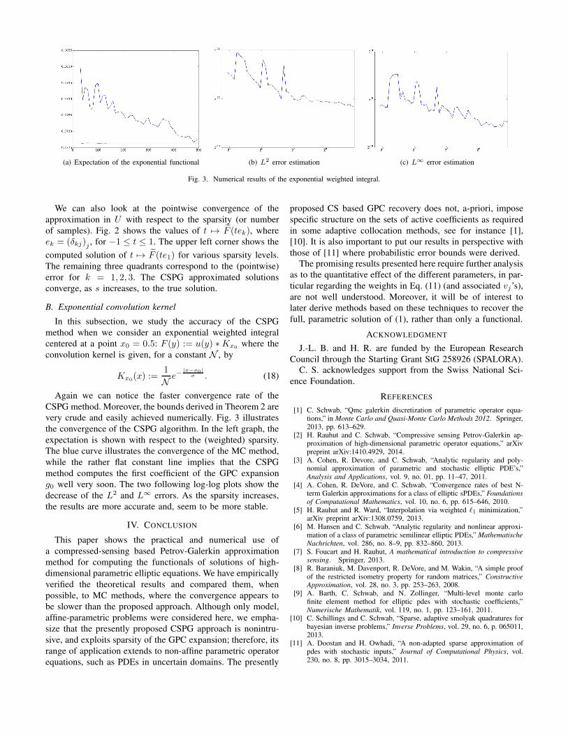
(a) Expectation of the exponential functional (b) L2 error estimation (c) L∞ error estimation

Fig. 3. Numerical results of the exponential weighted integral.

We can also look at the pointwise convergence of the

approximation in U with respect to the sparsity (or number

of samples). Fig. 2 shows the values of t 7→ F (tek), where

ek = (δkj)j , for −1 ≤ t ≤ 1. The upper left corner shows the

computed solution of t 7→ F (te1) for various sparsity levels.

The remaining three quadrants correspond to the (pointwise)

error for k = 1, 2, 3. The CSPG approximated solutions

converge, as s increases, to the true solution.

B. Exponential convolution kernel

In this subsection, we study the accuracy of the CSPG

method when we consider an exponential weighted integral

centered at a point x0 = 0.5: F (y) := u(y) ∗Kx0where the

convolution kernel is given, for a constant N , by

Kx0(x) :=

1

N e−|x−x0|

σ . (18)

Again we can notice the faster convergence rate of the

CSPG method. Moreover, the bounds derived in Theorem 2 are

very crude and easily achieved numerically. Fig. 3 illustrates

the convergence of the CSPG algorithm. In the left graph, the

expectation is shown with respect to the (weighted) sparsity.

The blue curve illustrates the convergence of the MC method,

while the rather flat constant line implies that the CSPG

method computes the first coefficient of the GPC expansion

g0 well very soon. The two following log-log plots show the

decrease of the L2 and L∞ errors. As the sparsity increases,

the results are more accurate and, seem to be more stable.

IV. CONCLUSION

This paper shows the practical and numerical use of

a compressed-sensing based Petrov-Galerkin approximation

method for computing the functionals of solutions of high-

dimensional parametric elliptic equations. We have empirically

verified the theoretical results and compared them, when

possible, to MC methods, where the convergence appears to

be slower than the proposed approach. Although only model,

affine-parametric problems were considered here, we empha-

size that the presently proposed CSPG approach is nonintru-

sive, and exploits sparsity of the GPC expansion; therefore, its

range of application extends to non-affine parametric operator

equations, such as PDEs in uncertain domains. The presently

proposed CS based GPC recovery does not, a-priori, impose

specific structure on the sets of active coefficients as required

in some adaptive collocation methods, see for instance [1],

[10]. It is also important to put our results in perspective with

those of [11] where probabilistic error bounds were derived.

The promising results presented here require further analysis

as to the quantitative effect of the different parameters, in par-

ticular regarding the weights in Eq. (11) (and associated vj’s),

are not well understood. Moreover, it will be of interest to

later derive methods based on these techniques to recover the

full, parametric solution of (1), rather than only a functional.

ACKNOWLEDGMENT

J.-L. B. and H. R. are funded by the European Research

Council through the Starting Grant StG 258926 (SPALORA).

C. S. acknowledges support from the Swiss National Sci-

ence Foundation.

REFERENCES

[1] C. Schwab, “Qmc galerkin discretization of parametric operator equa-tions,” in Monte Carlo and Quasi-Monte Carlo Methods 2012. Springer,2013, pp. 613–629.

[2] H. Rauhut and C. Schwab, “Compressive sensing Petrov-Galerkin ap-proximation of high-dimensional parametric operator equations,” arXivpreprint arXiv:1410.4929, 2014.

[3] A. Cohen, R. Devore, and C. Schwab, “Analytic regularity and poly-nomial approximation of parametric and stochastic elliptic PDE’s,”Analysis and Applications, vol. 9, no. 01, pp. 11–47, 2011.

[4] A. Cohen, R. DeVore, and C. Schwab, “Convergence rates of best N-term Galerkin approximations for a class of elliptic sPDEs,” Foundations

of Computational Mathematics, vol. 10, no. 6, pp. 615–646, 2010.[5] H. Rauhut and R. Ward, “Interpolation via weighted ℓ1 minimization,”

arXiv preprint arXiv:1308.0759, 2013.[6] M. Hansen and C. Schwab, “Analytic regularity and nonlinear approxi-

mation of a class of parametric semilinear elliptic PDEs,” Mathematische

Nachrichten, vol. 286, no. 8–9, pp. 832–860, 2013.[7] S. Foucart and H. Rauhut, A mathematical introduction to compressive

sensing. Springer, 2013.[8] R. Baraniuk, M. Davenport, R. DeVore, and M. Wakin, “A simple proof

of the restricted isometry property for random matrices,” ConstructiveApproximation, vol. 28, no. 3, pp. 253–263, 2008.

[9] A. Barth, C. Schwab, and N. Zollinger, “Multi-level monte carlofinite element method for elliptic pdes with stochastic coefficients,”Numerische Mathematik, vol. 119, no. 1, pp. 123–161, 2011.

[10] C. Schillings and C. Schwab, “Sparse, adaptive smolyak quadratures forbayesian inverse problems,” Inverse Problems, vol. 29, no. 6, p. 065011,2013.

[11] A. Doostan and H. Owhadi, “A non-adapted sparse approximation ofpdes with stochastic inputs,” Journal of Computational Physics, vol.230, no. 8, pp. 3015–3034, 2011.

Recent Research Reports

Nr. Authors/Title

2014-39 P. Grohs and M. SprecherTotal Variation Regularization by Iteratively Reweighted Least Squares on HadamardSpaces and the Sphere

2014-40 R. Casagrande and R. HiptmairAn A Priori Error Estimate for Interior Penalty Discretizations of the Curl-CurlOperator on Non-Conforming Meshes

2015-01 X. Claeys and R. HiptmairIntegral Equations for Electromagnetic Scattering at Multi-Screens

2015-02 R. Hiptmair and S. SargheiniScatterers on the substrate: Far field formulas

2015-03 P. Chen and A. Quarteroni and G. RozzaReduced order methods for uncertainty quantification problems

2015-04 S. Larsson and Ch. SchwabCompressive Space-Time Galerkin Discretizations of Parabolic Partial

Differential Equations

2015-05 S. MayNew spacetime discontinuous Galerkin methods for solving convection-diffusionsystems

2015-06 H. Heumann and R. Hiptmair and C. PagliantiniStabilized Galerkin for Transient Advection of Differential Forms

2015-07 J. Dick and F.Y. Kuo and Q.T. Le Gia and Ch. SchwabFast QMC matrix-vector multiplication