Comprehensive Master Drainage Plans

John E. F isher Civil Engineer

Clyde E. Williams & Associates, Inc.South Bend, Indiana

IN T R O D U C T IO N

Comprehensive master drainage plans are not a new concept in engineering. Engineers for decades have been planning drainage projects encompassing many of the facts of what is called comprehensive plan­ning. The difference between the past and the present is the availability of high speed computers and that now these facets have to be included and documented for public and private acceptance and review. The reason for this is because of the advent of public awareness in our environment. I t is not uncommon now to read in the newspapers that another public works project has been stalemated because of interven­tion of a conservation group or another member of the private sector.

W ith this and with the advent of systems analysis and the high speed computer, comprehensive water drainage plans have formally ar­rived. A comprehensive master drainage plan is a formulation of the drainage problems now and those expected in the future and the sub­sequent testing of recommended alternatives with respect to any com­bination of or all of the following variables: geologic, geographic,topographic, hydrologic, hydraulic, ecologic, socio-economic, transporta­tion, sedimentation and erosion, political, soils, operation and mainte­nance, construction methods and materials, planning, present and future land use, and zoning.

After the alternatives are tested, one or more are selected as feasible and recommended and a project implementation schedule is formulated.

There is no question that this type of formal approach to drainage problems is here to stay. Currently the federal government and other governmental entities are funding research projects of this type all over the country. Most commonly, these research projects are oriented to­ward urban drainage problems and are funded through the W ater Resources Research Act of 1964, Title I and T itle II and the Depart­ment of Housing and Urban Development 701 (b) program. Today’s scientific and technologic literature is filled with articles on various

150

151

aspects of this type of study. The literature of the American Geo­physical Union, the American W ater Resources Association, the Amer­ican Society of Civil Engineers, the American Public Works Association and the various agencies of the Federal Government is typical of the abundance of this type of article.

This paper will treat one particular approach to a comprehensive master drainage plan; the simulation approach. The simulation ap­proach is a technique whereby a physical system is simulated mathe­matically usually by a high speed digital computer. The advantage of a similation technique is that inputs of different magnitudes of different variables can be simulated rather rapidly on a computer and their effects can be seen and evaluated immediately. In this way, more alter­natives and would-be constraints are analyzed in less time than a stand­ard empirical engineering analysis. For example, using the computer program developed in this study, a rainfall of given frequency and duration can be simulated on a basin of about 20,000 acres in less than three minutes with resultant output of hydrographs at 45 locations in the basin and corresponding depths of flow and runoff volumes. The computer cost for this simulation would be about $66. This does not include the payroll cost of an engineer to code the data, run the com­puter, or evaluate the output.

S IM U L A T IO N M E T H O DThis paper will describe a drainage study including simulation made

by Clyde E. Williams & Associates, Inc., for the St. Joseph County Area Plan Commission. The study consisted of the following six elements:

S i x E l e m e n t s o f t h e D r a i n a g e S t u d y

1) Field Data Collection. Between April 1969 and July 1970 several field crews obtained a variety of measurements and data related to this study. This information consisted of: a) the typical slopes, cross sections, and condition of principal segments of water courses within the country; b) the location, geometric configuration, and condition of principal drainage structures such as road culverts, bridges, etc., within the country; c) stream gaging data at several points along water courses within the county determining stream dis­charges (rates of flow) under a variety of weather conditions; and d) precipitation measurements at various times and locations within the county.

2) Map Preparation. Base maps of the county, at a scale of one inch equal 3000 feet, were available from the Area Plan Commission

152

at the outset of this study. U.S.G.S. quadrangle maps were also avail­able and some soils mapping had been completed by the U.S.D.A. Soil Conservation Service. These existing maps were examined and devel­oped into the maps employed as working sheets and presentation sheets for this report. The one inch equal 3000 feet general base map was used for delineation and depiction of current zoning, proposed land use, soils type, and watershed areas of the county. The individual watershed areas, once defined on the general large scale base map, are presented individually on enlarged views (one inch equals 600 feet) of these base map areas. Drainage courses, drainage structures, computer sta­tions, and other pertinent drainage factors are indicated on these water­shed maps.

3) Computer Programming. In order to achieve the objectives of this study, it was determined that the complex interrelationship of the many hydrologic factors pertinent to the drainage flow of the county required analysis by computerized techniques. A computer program was written, in Fortran V scientific and engineering language, which al­lowed the determination of rate of How at any selected set of points along a watercourse or watercourses, at any selected set of consecutive time intervals. The plot of these flow rates against time for each selected point is termed a “flow hydrograph” for that point.

These hydrographs form the basic data upon which analysis, cost estimating, and recommendations have been formulated.

The input required for the completed computer program consists of the significant hydrologic factor data which affects runoff flow. Namely, this information is the intensity and duration of the precipita­tion, the land use for each sub-area of the watershed, the geometry (length and land slope) of each sub-area of the watershed, the geometry (cross section and slope) of each principal segment of the stream, and the hydraulic factors of the stream segments. This data is chained together into a drainage network in the program through a number cod­ing system. Runoff flows are determined at upstream ends of branches of the network; these flows are routed to the next station downstream where the routed flow is then summed with the additional network sub- area runoff contribution, and so on, until the terminal station of the network has been reached. The program thus “simulates” the drainage flow patterns of the watershed, and is termed a simulation program.

4) Computer Program Calibration. In order to establish reason­able precision of the simulated drainage flows generated by the computer program, calibration of the program was required. This was accom­plished through successive modification of significant parameters for

153

individual computer runs until the generated hydrographs for a given precipitation event agreed within tolerable limits with the actual field measured hydrographs for that event. The parameters which were varied in the calibration procedure included the time of concentration of watershed sub-areas, the runoff coefficients of the watershed sub-areas, the bank storage capacity of certain watercourse segments, the shape of individual sub-area runoff hydrographs, and the empirically modified hydrograph translation along poorly defined channels.

5) Runoff and Drainage Flow Forecasts. Computer output was obtained for a variety of storm types on each watershed area. On each watershed, certain sub-areas are especially sensitive to short duration storms while the principal drainage course of the watershed might have been more critically affected by longer duration precipitation. There­fore, analysis of the effects of the various types of storms was required and was accomplished. The basic storm chosen for the analyses was one of ten-year-recurrence intervals on the basis that the relatively high valued development of the county be afforded this minimum flood pro­tection level. In some instances, existing or inexpensive modification to existing drainage patterns permitted protection against more intense flooding and advantage was taken of these situations.

6 ) Cost Estimates and Recommendations. The cost of proposed drainage improvements and the priority schedule of each were com­pleted and these are given for each watershed area.

J u d y C r e e k W a t e r s h e d U s e d f o r C a l i b r a t i o n S t u d y o f R u r a l A r e a s

There were seven basins studied in detail. This paper will consider one of these as typical of the other seven, with one exception; the Clyde Creek Basin. The Clyde Creek Basin is not typical or similar to the others in that it is developed much more into urban areas. This difference will be shown subsequently in the summary where the costs for solving the existing and proposed drainage problems are given.

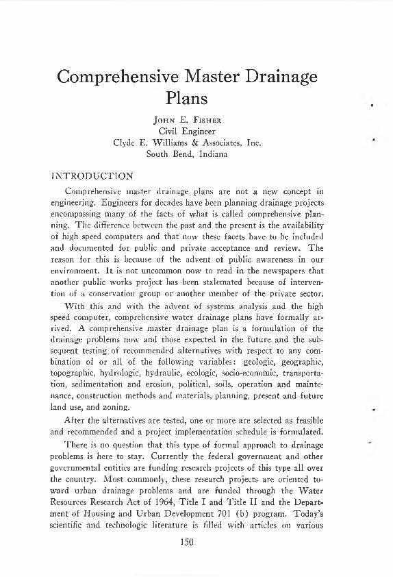
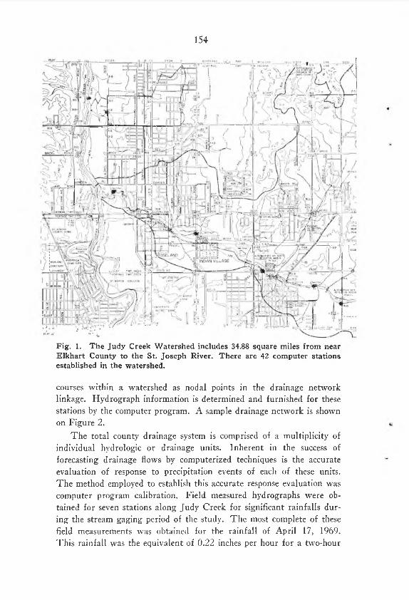
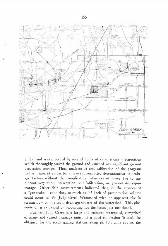
The Judy Creek Watershed is situated along the northern limit of the City of South Bend. This is the largest watershed area in the intensive study area, totaling 34.88 square miles. Judy Creek flows generally from east to west from nearly the Elkhart County line to the St. Joseph River, terminating at a point between Cleveland and Darden Roads. I t is an open channel for its full length except for some culvert structures beneath roadways. The Judy Creek Watershed is shown in Figure 1.

The computer program developed for this study is organized so as to require the denoting of certain selected stations along drainage

154

Fig. 1. The Judy Creek Watershed includes 34.88 square miles from near Elkhart County to the St. Joseph River. There are 42 computer stations established in the watershed.

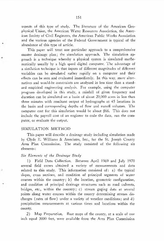
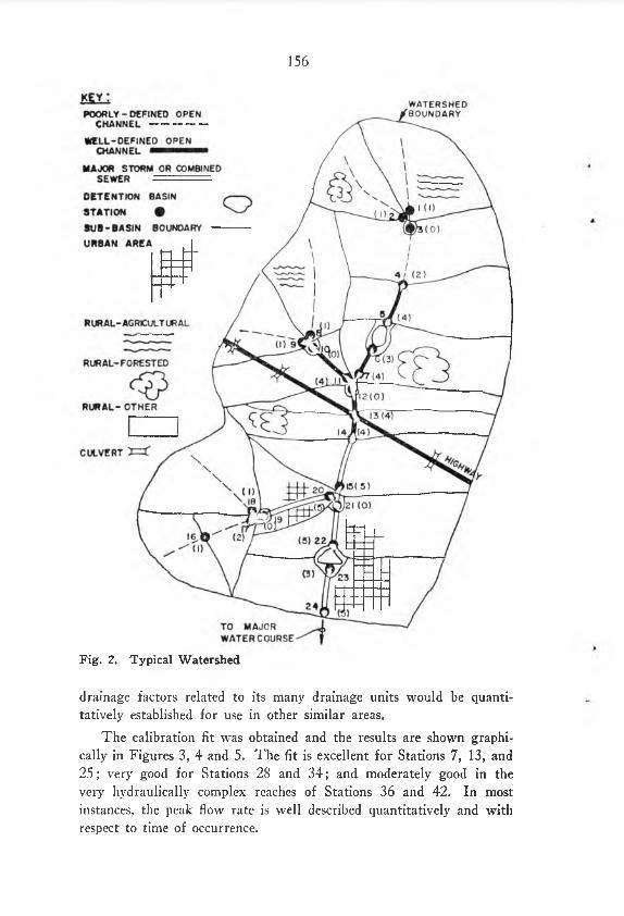
courses within a watershed as nodal points in the drainage network linkage. Hydrograph information is determined and furnished for these stations by the computer program. A sample drainage network is shown on Figure 2.

The total county drainage system is comprised of a multiplicity of individual hydrologic or drainage units. Inherent in the success of forecasting drainage flows by computerized techniques is the accurate evaluation of response to precipitation events of each of these units. The method employed to establish this accurate response evaluation was computer program calibration. Field measured hydrographs were ob­tained for seven stations along Judy Creek for significant rainfalls dur­ing the stream gaging period of the study. The most complete of these field measurements was obtained for the rainfall of April 17, 1969. This rainfall was the equivalent of 0.22 inches per hour for a two-hour

155

period and was preceded by several hours of slow, steady precipitation which thoroughly soaked the ground and usurped any significant ground depression storage. Thus, analyses of and calibration of the program

< to the measured values for this event permitted determination of drain­age factors without the complicating influences of losses due to sig­nificant vegetation interception, soil infiltration, or ground depression

* storage. Other field measurements indicated that, in the absence ofa “pre-soaked” condition, as much as 0.5 inch of precipitation volume could occur on the Judy Creek Watershed with no apparent rise in stream flow on the main drainage courses of the watershed. This phe­nomenon is explained by accounting for the losses just mentioned.

Further, Judy Creek is a large and complex watershed, comprised of many and varied drainage units. If a good calibration fit could be obtained for the seven gaging stations along its 1 0 . 5 mile course, the

1 5 6

Fig. 2. Typical Watershed

drainage factors related to its many drainage units would be quanti­tatively established for use in other similar areas.

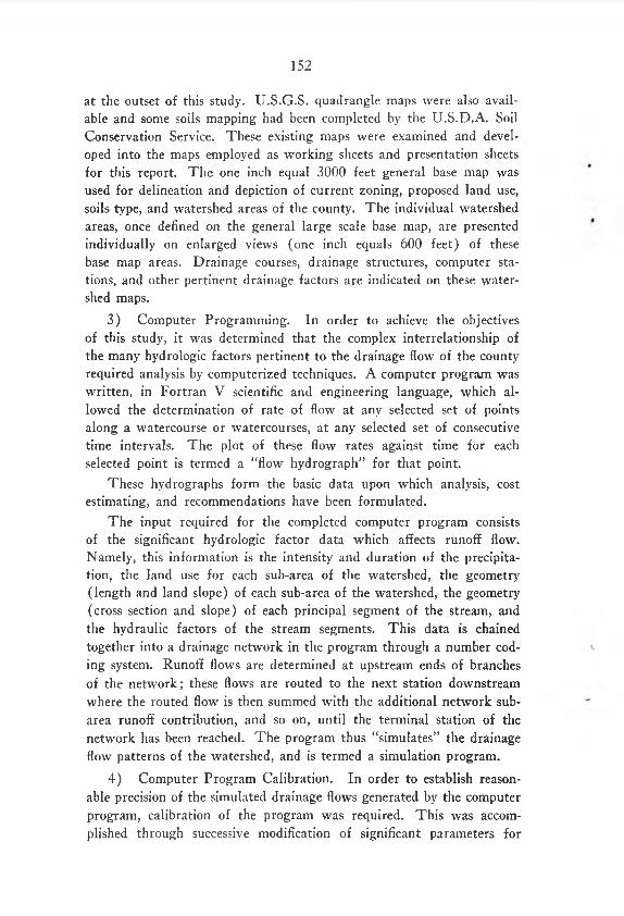
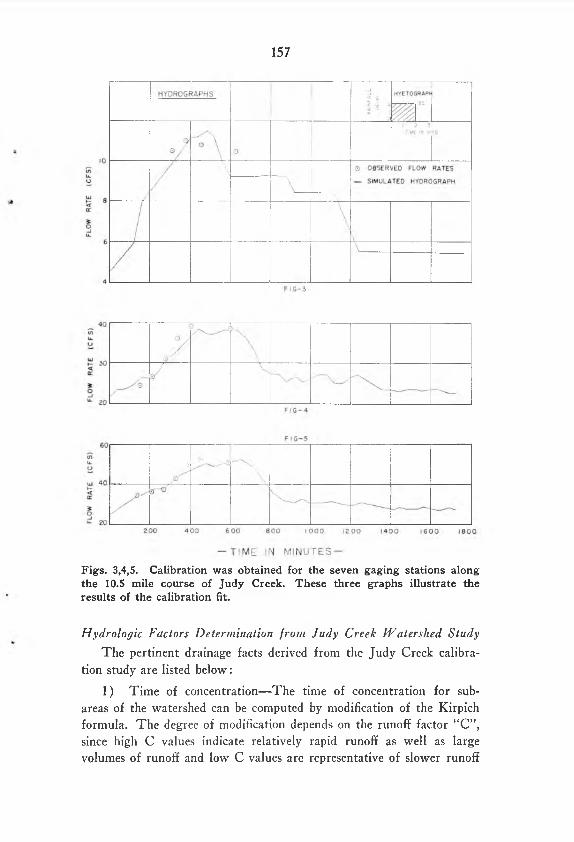
The calibration fit was obtained and the results are shown graphi­cally in Figures 3, 4 and 5. The fit is excellent for Stations 7, 13, and 25; very good for Stations 28 and 34; and moderately good in the very hydraulically complex reaches of Stations 36 and 42. In most instances, the peak flow rate is well described quantitatively and with respect to time of occurrence.

157

Figs. 3,4,5. Calibration was obtained for the seven gaging stations along the 10.5 mile course of Judy Creek. These three graphs illustrate the results of the calibration fit.

H y d r o l o g i c F a c t o r s D e t e r m i n a t i o n f r o m J u d y C r e e k W a t e r s h e d S t u d y

The pertinent drainage facts derived from the Judy Creek calibra­tion study are listed below:

1) Time of concentration—The time of concentration for sub- areas of the watershed can be computed by modification of the Kirpich formula. The degree of modification depends on the runoff factor “C”, since high C values indicate relatively rapid runoff as well as large volumes of runoff and low C values are representative of slower runoff

158

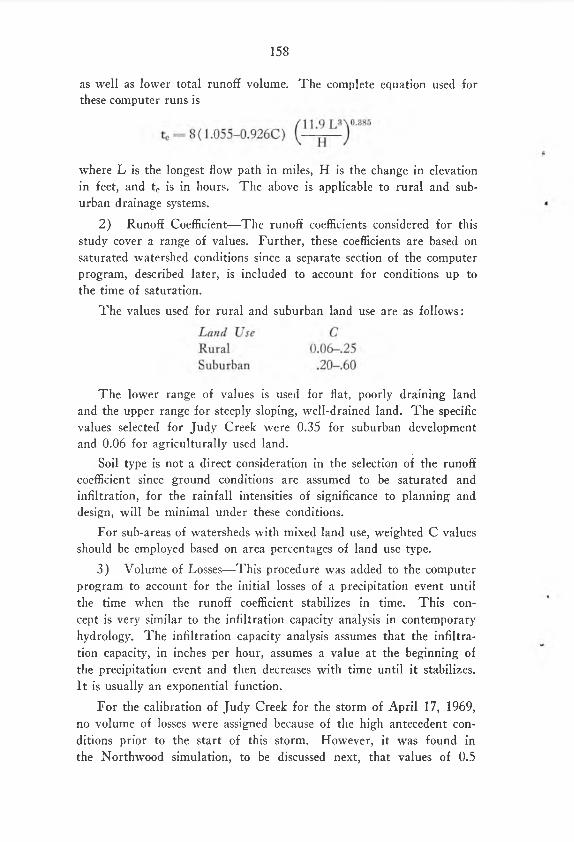
as well as lower total runoff volume. The complete equation used for these computer runs is

where L is the longest flow path in miles, H is the change in elevation in feet, and tc is in hours. The above is applicable to rural and sub­urban drainage systems.

2) Runoff Coefficient—The runoff coefficients considered for this study cover a range of values. Further, these coefficients are based on saturated watershed conditions since a separate section of the computer program, described later, is included to account for conditions up to the time of saturation.

The values used for rural and suburban land use are as follows:

The lower range of values is used for flat, poorly draining land and the upper range for steeply sloping, well-drained land. The specific values selected for Judy Creek were 0.35 for suburban development and 0.06 for agriculturally used land.

Soil type is not a direct consideration in the selection of the runoff coefficient since ground conditions are assumed to be saturated and infiltration, for the rainfall intensities of significance to planning and design, will be minimal under these conditions.

For sub-areas of watersheds with mixed land use, weighted C values should be employed based on area percentages of land use type.

3) Volume of Losses—This procedure was added to the computer program to account for the initial losses of a precipitation event until the time when the runoff coefficient stabilizes in time. This con­cept is very similar to the infiltration capacity analysis in contemporary hydrology. The infiltration capacity analysis assumes that the infiltra­tion capacity, in inches per hour, assumes a value at the beginning of the precipitation event and then decreases with time until it stabilizes. It is usually an exponential function.

For the calibration of Judy Creek for the storm of April 17, 1969, no volume of losses were assigned because of the high antecedent con­ditions prior to the start of this storm. However, it was found in the Northwood simulation, to be discussed next, that values of 0.5

159

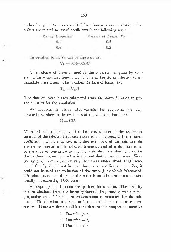
inches for agricultural area and 0.2 for urban area were realistic. These values are related to runoff coefficients in the following way:

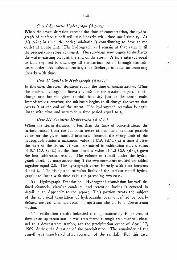
The volume of losses is used in the computer program by com­puting the equivalent time it would take at the storm intensity to ac­cumulate these losses. This is called the time of losses, T L.

The time of losses is then subtracted from the storm duration to give the duration for the simulation.

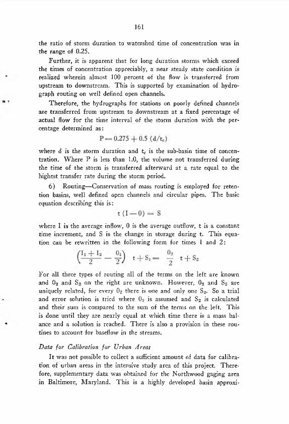
4) Hydrograph Shape—Hydrographs for sub-basins are con­structed according to the principles of the Rational Formula:

Where Q is discharge in CFS to be expected once in the recurrence interval of the selected frequency storm to be analyzed, C is the runoff coefficient, i is the intensity, in inches per hour, of the rain for the recurrence interval of the selected frequency and of a duration equal to the time of concentration for the watershed contributing area for the location in question, and A is the contributing area in acres. Since the rational formula is only valid for areas under about 1,000 acres and definitely should not be used for areas over five square miles, it could not be used for evaluation of the entire Judy Creek Watershed. Therefore, as explained before, the entire basin is broken into sub-basins usually not exceeding 1,000 acres.

A frequency and duration are specified for a storm. The intensity is then obtained from the intensity-duration-frequency curves for the geographic area. The time of concentration is computed for the sub­basin. The duration of the storm is compared to the time of concen­tration. There are three possible conditions to this comparison, namely:

I Duration > tcII Duration = tcIII Duration < tc

160

C a s e I S y n t h e t i c H y d r o g r a p h ( d > t c)

When the storm duration exceeds the time of concentration, the hydro­graph of surface runoff will rise linearly with time until time tc. At this point in time, the entire sub-basin is contributing to flow at the outlet at a rate CiA. The hydrograph will remain at that value until the precipitation stops at time d. The sub-basin now begins to discharge the water existing on it at the end of the storm. A time interval equal to tc is required to discharge all the surface runoff through the sub­basin outlet. As indicated earlier, that discharge is taken as occurring linearly with time.

C a s e I I S y n t h e t i c H y d r o g r a p h ( d = t c)

In this case, the storm duration equals the time of concentration. Thus the outflow hydrograph linearly climbs to the maximum possible dis­charge rate for the given rainfall intensity just as the storm ends. Immediately thereafter, the sub-basin begins to discharge the water that covers it at the end of the storm. The hydrograph recession is again linear with time and occurs in a time period equal to tc.

C a s e I I I S y n t h e t i c H y d r o g r a p h ( d < t c)

When the storm duration is less than the time of concentration, the surface runoff from the sub-basin never attains the maximum possible value for the given rainfall intensity. Instead, the rising limb of the hydrograph attains a maximum value of CiA (d / tc) at a time d after the start of the storm. It was determined in calibration that a value of 0.7 CiA (c /tc) at the time d and a value of 1.3 CiA (d / tc) gave the best calibration results. The volume of runoff under the hydro­graph checks by mass accounting if the two coefficient multipliers added together equal 2.0. The hydrograph varies linearly with time between d and tc. The rising and recession limbs of the surface runoff hydro­graph are linear with time as in the preceding two cases.

5) Hydrograph Translation— Hydrograph translation for well de­fined channels, circular conduits, and retention basins is covered in detail in an Appendix to the report. This portion treats the subject of the empirical translation of hydrographs over undefined or poorly defined natural channels from an upstream station to a downstream station.

The calibration results indicated that approximately 40 percent of flow at an upstream station was transferred through an undefined chan­nel to a downstream station, for the precipitation event of April 17, 1969, during the duration of the precipitation. The remainder of the runoff was transferred after secession of the rainfall. For this case,

161

the ratio of storm duration to watershed time of concentration was in the range of 0.25.

Further, it is apparent that for long duration storms which exceed the times of concentration appreciably, a near steady state condition is realized wherein almost 1 0 0 percent of the flow is transferred from upstream to downstream. This is supported by examination of hydro­graph routing on well defined open channels.

Therefore, the hydrographs for stations on poorly defined channels are transferred from upstream to downstream at a fixed percentage of actual flow for the time interval of the storm duration with the per­centage determined as:

where d is the storm duration and tc is the sub-basin time of concen­tration. Where P is less than 1.0, the volume not transferred during the time of the storm is transferred afterward at a rate equal to the highest transfer rate during the storm period.

6 ) Routing— Conservation of mass routing is employed for reten­tion basins, well defined open channels and circular pipes. The basic equation describing this is:

where I isi the average inflow, 0 is the average outflow, t is a constant time increment, and S is the change in storage during t. This equa­tion can be rewritten in the following form for times 1 and 2 :

For all three types of routing all of the terms on the left are known and O2 and S2 on the right are unknown. However, 0 2 and S2 are uniquely related, for every 0 2 there is one and only one S2. So a trial and error solution is tried where 0 2 is assumed and S2 is calculated and their sum is compared to the sum of the terms on the left. This is done until they are nearly equal at which time there is a mass bal­ance and a solution is reached. There is also a provision in these rou­tines to account for baseflow in the streams.

D a t a f o r C a l i b r a t i o n f o r U r b a n A r e a s

I t was not possible to collect a sufficient amount of data for calibra­tion of urban areas in the intensive study area of this project. There­fore, supplementary data was obtained for the Northwood gaging area in Baltimore, Maryland. This is a highly developed basin approxi-

162

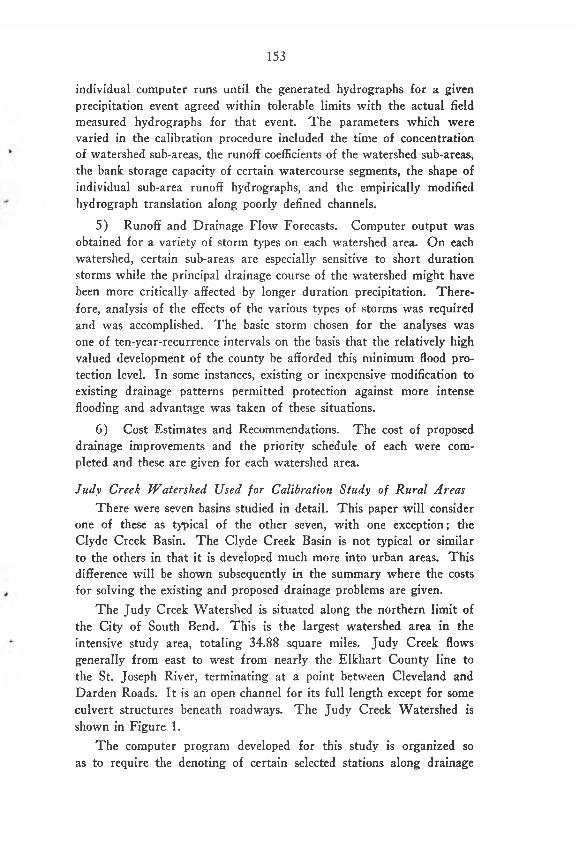
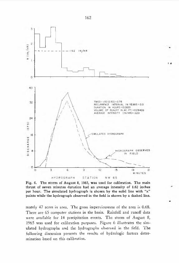
Fig. 6. The storm of August 8, 1965, was used for calibration. The main thrust of seven minutes duration had an average intensity of 1.62 inches per hour. The simulated hydrograph is shown by the solid line with “x” points while the hydrograph observed in the field is shown by a dashed line.

mately 47 acres in area. The gross imperviousness of the area is 0 .6 8 . There are 65 computer stations in the basin. Rainfall and runoff data were available for 14 precipitation events. The storm of August 8 , 1965 was used for calibration purposes. Figure 6 illustrates the sim­ulated hydrographs and the hydrographs observed in the field. The following discussion presents the results of hydrologic factors deter­mination based on this calibration.

163

H y d r o lo g ic F a c to r s D e te r m in a t io n B a s e d on U r b a n A r e a C a l ib r a t io n

1) Time of Concentration— The time of concentration for sub­basins of the fully developed urban type is computed as a modification of the Kirpich formula. The modification is again a function of the runoff coefficient, C. The formula used is:

where L is the longest flow path in miles, H is the change in elevation in feet, C is the runoff coefficient, and tc is the time of concentration in hours.

2) Runoff Coefficient— The gross imperviousness of this area is reported as 0.68. The average ground slope is about three percent. The following range of C values was considered.

Runoff coefficients were assigned depending on the sub-basin land use. The average C value used, weighted with respect to area, was 0.68. There again, the lower range of C values is used for flat, poorly drain­ing land and the upper range for steeply sloping well drained land. Where there is mixed land use in a sub-basin, the net C is weighted with respect to area.

3) Volume of Losses— The main thrust of the storm fell in the first seven minutes. The entire first two minutes of the storm were considered to be lost to interception and depression storage. Sixty-seven percent of the precipitation for the next five minutes was averaged to give an intensity of 1.62 inches per hour for five minutes as the average intensity and duration used in STM 55. For the entire first seven min­utes this means that 55 percent of the total precipitation was used in a five minute duration in the simulation program. There was .04 inches of antecedent precipitation in the preceding 24 hours.

4) Hydrograph Shape— same as for suburban and rural area.

5) Hydrograph Translation— same as for suburban and ruralareas.

6) Routing— same as for suburban and rural areas. For a typical drainage study a certain minimum acceptable design frequency is first selected. This is usually ten years. Once this is determined a series of storms of this recurrence interval with varying durations are simulated for the existing basin. The purpose of this series is to determine the

164

critical times of concentration of the various points on the watershed. The most critical storm for discharge capacity design is the storm which gives the highest Q-peak’s, and flooding conditions and thus evaluate the economics of providing protection for this future development. This determination is usually made on a benefit-cost basis. A series of simu­lations is then made with a higher frequency storm on the future con­dition of the basin to see if it might be more economical to provide this higher frequency protection via a benefit-cost analysis.

T h e F u n d a m e n t a l C o n s t r a i n t in J u d y C r e e k W a t e r s h e d

The Judy Creek Basin is composed of 36.5 square miles, or 22,322 acres. Judy Creek is a tributary of the St. Joseph River which is a tributary to Lake Michigan. The length of the main channel from where it becomes well defined to its mouth is about 10.5 miles. The watershed and stream are delineated in Figure 1. Existing drainage structures are indicated on the table attached. Approximately 7.8 square miles or 21 percent of the watershed is located in Berrien County, Michigan. The headwaters of the stream originate in this area. The stream itself flows basically in a westward direction from EN E of the intersection of the Indiana Toll Road and Bittersweet Road to its mouth south of the Darden Road Bridge on the Isaac Walton League property. The average baseflow of the stream ranges from, about 5 cfs in its upper reaches to 25 cfs in its lower reaches. The average slope of the main channel is about 0.4 percent. There are no major tributaries.

Seven stream gages were established on Judy Creek in April 1969. There are 42 computer stations established in the watershed. Delinea­tion of these is shown in Figure 1.

The relief of the basin ranges from about elevation 800 at the upstream drainage divide to 670 at the mouth of the stream. All eleva­tions are U.S.G.S. datum. There are no major topographic features in the basin.

The soils in the basin are mainly sands with a high ground water table. The baseflow of Judy Creek is a groundwater contribution. The soils fall into Group Classification Nos. I, II, VI and V II. (Refer­ence: Soil Conservation Service Soils Study of St. Joseph County.)

Approximately 70 percent of the watershed is still agricultural with about 30 percent being low to medium density urban development. The land adjoining the stream in approximately its lower one-third is highly developed with a semi-sparse residential development. Consequently, there are many artificial controls on this part of the stream such as

165

weirs, dams, diversions, bridges and small rapids. These controls make the hydrologic and hydraulic analysis of the stream very difficult.

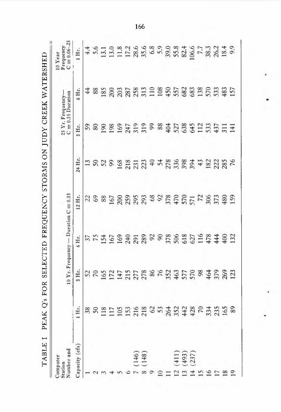
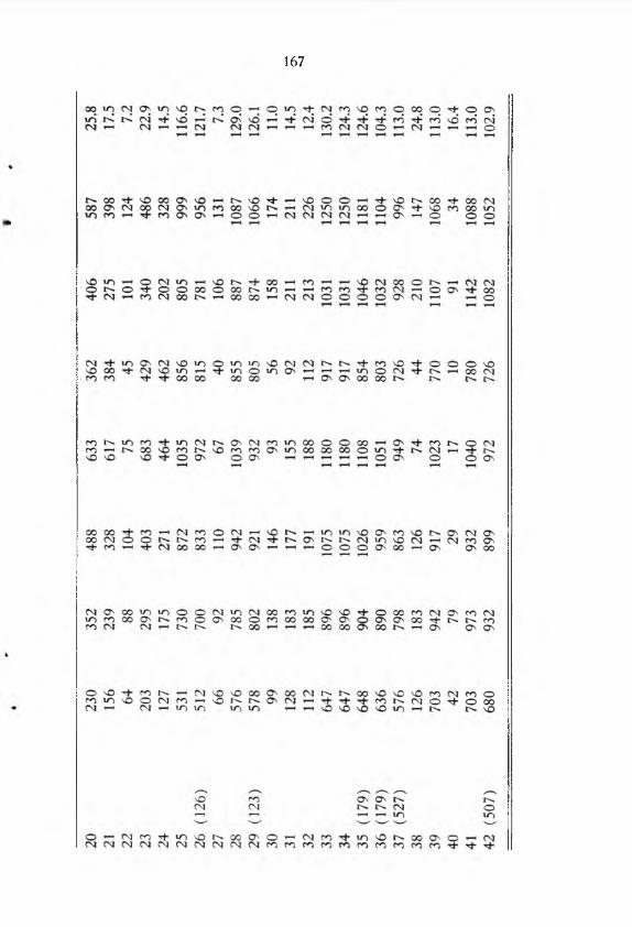
The storm of April 17, 1969 starting at 4 p.m. was used to cali­brate the drainage simulation computer program STM 55 for the Judy Creek Watershed. Other storms were monitored in the basin but in­sufficient data were gathered. Besides the calibration storm a series of eight other storms was run on the basin. Table I gives the peak dis­charge values, Q-peak, for each of the 42 computer stations for each of the storms. A ten-year, one-hour storm was simulated on the exist­ing basin as it is today. Next a series of ten-year storms was simulated on the basin as it will be hydrologically in the future. These simula­tions show the effect of changing the land use from agricultural to low density urban development. This means that the runoff coefficient changes from 0.06 to 0.35 based on calibration results. The five differ­ent duration-1 0 -year storms were run to determine the critical duration storm or time of concentration for each computer station. The critical duration storm is the storm which gives the highest Q-peak usually felt somewhere between three and six hours, so the three-hour and six-hour 25-year storms were simulated.

Analysis of the Judy Creek Watershed indicates that the funda­mental constraint of this drainage system is the Judy Creek channel capacity in the section approximately between Grape Road and Juniper Road. This segment of the channel has a present bank full capacity varying between approximately 125 and 180 cfs.

It is considered economically and esthetically infeasible to develop significantly greater channel capacity through the above-mentioned chan­nel segment.

The area is moderately well developed with residences of middle to high value bordering the stream. Because of this, it was considered that flow through this stream segment should be limited to the range of 200 cfs for the 10-year-recurrence interval-event. Such a criterion leads to the requirement of upstream storage in retention basins with a minimum of channel improvement, principally maintenance of banks and prevention of vegetation overgrowth, in the constrained segment.

D e v e l o p m e n t o f U p s tr e a ? n R e t e n t i o n B a s in A l t e r n a t i v e s

The development of the upstream retention basins was set out in three alternative systems and the systems were based on the ten-year storm-hydrograph forecasts obtained by computer runs.

166

TA

BL

E I

PE

AK

Q’s

FO

R S

EL

EC

TE

D F

RE

QU

EN

CY

ST

OR

MS

ON

JU

DY

CR

EE

K W

AT

ER

SH

ED

167

168

A l t e r n a t i v e N o . 1

This alternate is comprised chiefly of three large retention basins, increased channelization of the sub-basins, and structure improvements.

The three retention basins are proposed near the outlets of sub­basins numbers 11, 24, and 32.

The three proposed retention basins are designed for complete tem­porary storage of the ten-year storms. It should be noted that this provides flood protection for the 25-year, three- and six-hour storms as well.

It is planned that all land necessary for development of the basins for future conditions will be acquired now. However, only the volume needed for protection of the existing sub-basins is to be excavated now. The volume necessary for protection of the future development can be provided sequentially.

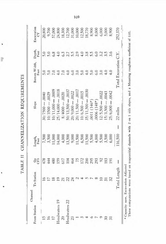
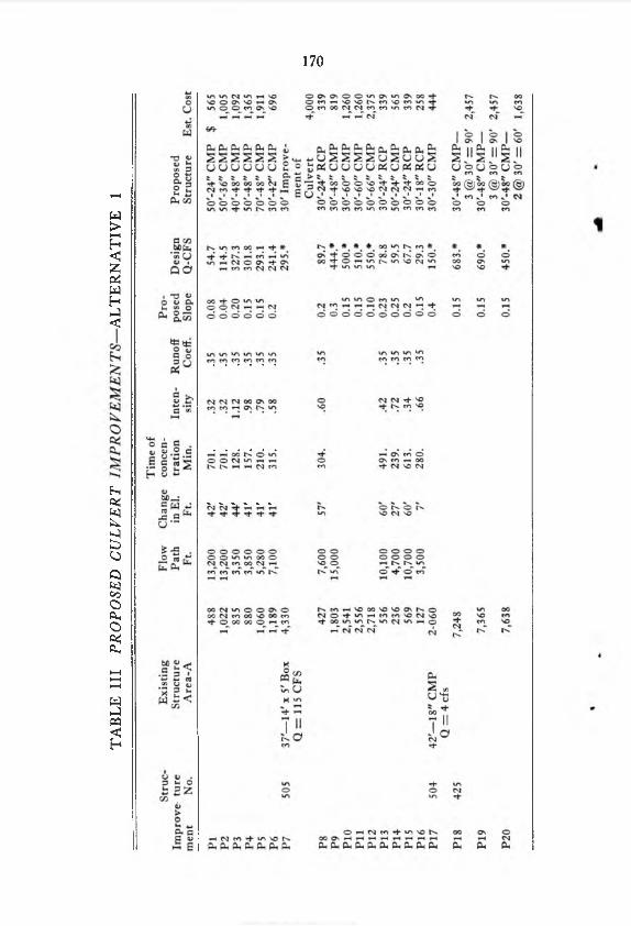
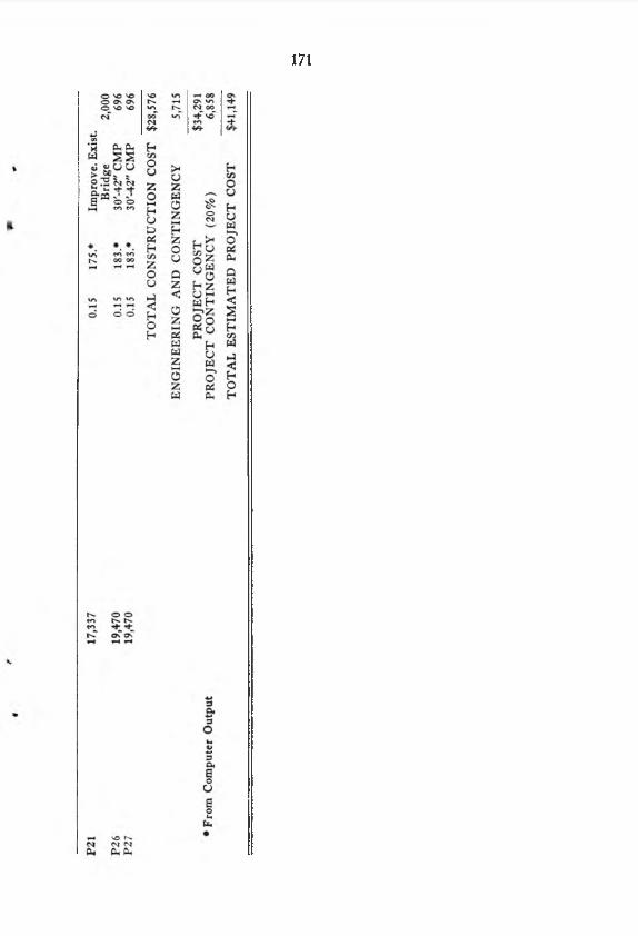
To make the three proposed retention basins completely functional, channelization is required according to Table II. For the proper func­tioning of the retention basins, channelization is required. For the proper functioning of the increased channel capacity, structure improve­ment is required. Table III is a summary of critical structures in the watershed. Their identification numbers refer to the structure numbers in Figure 1.

It is anticipated that these three retention basins would also be used for recreation purposes. This would enhance the benefits of this proposal.

A l t e r n a t i v e N o . 2

This alternate is composed of a number of smaller retention basins sized to contain runoff from small sub-basins within the watershed. Because they are smaller, they are more numerous. For cost analysis purposes a hypothetical sub-basin development of 1 0 0 acres is assumed. Based on the theory of the simulation program the following hydrologic factors would be typical.

Drainage Area: 100 acres Runoff Coefficient, future: 0.35 Length of Overland F low : 2950 feet Change in Elevation: 15 feet Time of Concentration: 165 minutes Volume of Losses: 0.35 inches

Based on this analysis of a typical 100 acre development, drainage structures would have to be designed to handle 37.4 cfs of discharge and the retention basin would have to be designed to hold 1 0 . 6 acre-

169T

AB

LE

II

CH

AN

NE

LIZ

AT

ION

RE

QU

IRE

ME

NT

S

170

TA

BL

E I

II

PR

OP

OS

ED

CU

LV

ER

T

IMPROVEMENTS AL

TE

RN

AT

IVE

1

171

172

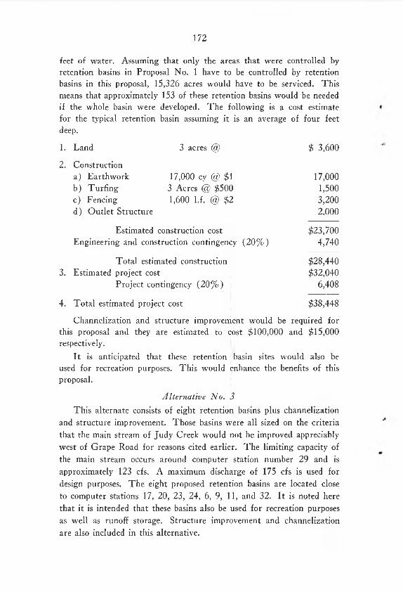
feet of water. Assuming that only the areas that were controlled by retention basins in Proposal No. 1 have to be controlled by retention basins in this proposal, 15,326 acres would have to be serviced. This means that approximately 153 of these retention basins would be needed if the whole basin were developed. The following is a cost estimate for the typical retention basin assuming it is an average of four feet deep.

1 . Land 3 acres @ $ 3,600

2 . Constructiona) Earthwork 17,000 cy @ $ 1 17,000b) Turfing 3 Acres @ $500 1,500c) Fencing 1,600 l.f. @ $ 2 3,200d) Outlet Structure 2 , 0 0 0

Estimated construction cost $23,700Engineering and construction contingency (20% ) 4,740

Total estimated construction $28,4403. Estimated project cost $32,040

Project contingency (20% ) 6,408

4. Total estimated project cost $38,448

Channelization and structure improvement would be required for this proposal and they are estimated to cost $ 1 0 0 , 0 0 0 and $15,000 respectively.

It is anticipated that these retention basin sites would also be used for recreation purposes. This would enhance the benefits of this proposal.

A l t e r n a t i v e N o . 3

This alternate consists of eight retention basins plus channelization and structure improvement. Those basins were all sized on the criteria that the main stream of Judy Creek would not be improved appreciably west of Grape Road for reasons cited earlier. The limiting capacity of the main stream occurs around computer station number 29 and is approximately 123 cfs. A maximum discharge of 175 cfs is used for design purposes. The eight proposed retention basins are located close to computer stations 17, 20, 23, 24, 6 , 9, 11, and 32. I t is noted here that it is intended that these basins also be used for recreation purposes as well as runoff storage. Structure improvement and channelization are also included in this alternative.

173

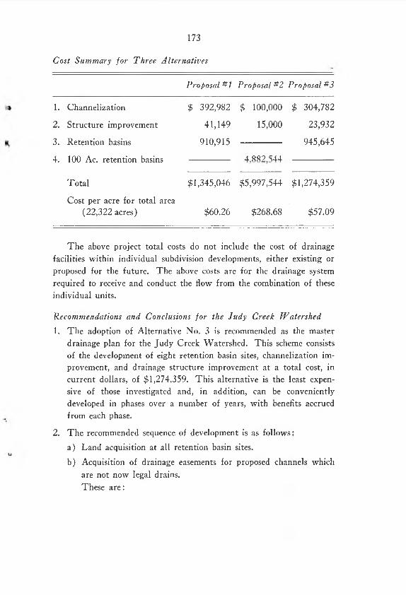
C o s t S u m m a r y f o r T h r e e A l t e r n a t i v e s

P r o p o s a l # 1 P r o p o s a l #2 P r o p o s a l # 3

1 . Channelization $ 392,982 $ 1 0 0 , 0 0 0 $ 304,782

2 . Structure improvement 41,149 15,000 23,932

3. Retention basins 910,915 945,645

4. 100 Ac. retention basins 4 8 8 ? S44

Total $1,345,046 $5,997,544 $1,274,359

Cost per acre for total area(22,322 acres) $60.26 $268.68 $57.09

The above project total costs do not include the cost of drainage facilities within individual subdivision developments, either existing or proposed for the future. The above costs are for the drainage system required to receive and conduct the flow from the combination of these individual units.

R e c o m m e n d a t i o n s a n d C o n c lu s io n s f o r th e J u d y C r e e k W a t e r s h e d

1. The adoption of Alternative No. 3 is recommended as the master drainage plan for the Judy Creek Watershed. This scheme consists of the development of eight retention basin sites, channelization im­provement, and drainage structure improvement at a total cost, in current dollars, of $1,274,359. This alternative is the least expen­sive of those investigated and, in addition, can be conveniently developed in phases over a number of years, with benefits accrued from each phase.

2. The recommended sequence of development is as follows:a) Land acquisition at all retention basin sites.

b) Acquisition of drainage easements for proposed channels which are not now legal drains.These are:

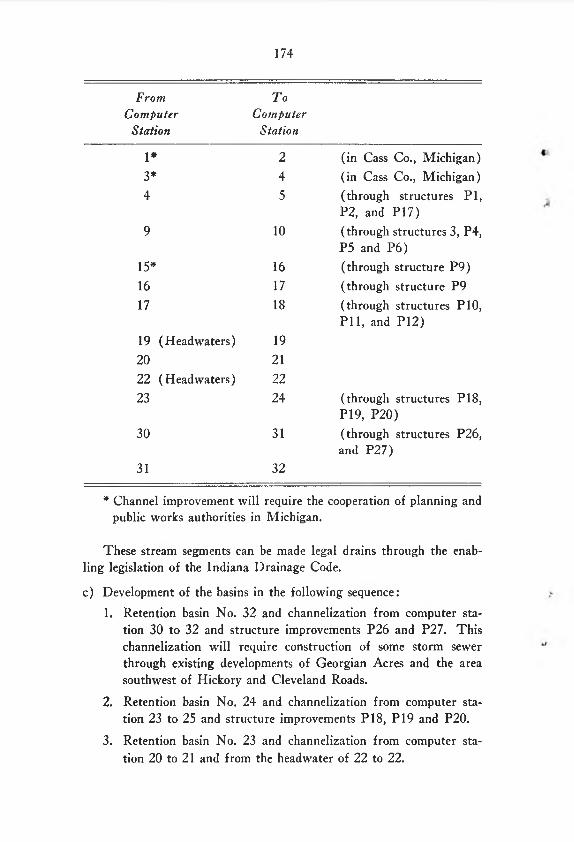
174

F r o m

C o m p u t e r

S t a t i o n

T o

C o m p u t e r

S t a t i o n

1* 2 (in Cass Co., Michigan)3* 4 (in Cass Co., Michigan)4 5 (through structures PI,

P2, and P17)9 1 0 (through structures 3, P4,

P5 and P 6 )15* 16 (through structure P9)16 17 (through structure P917 18 (through structures P 1 0 ,

P l l , and P12)19 (Headwaters) 19

2 0 2 1

22 (Headwaters) 2 2

23 24 (through structures P18, P19, P20)

30 31 (through structures P26, and P27)

31 32

* Channel improvement will require the cooperation of planning and public works authorities in Michigan.

These stream segments can be made legal drains through the enab­ling legislation of the Indiana Drainage Code.

c) Development of the basins in the following sequence:

1. Retention basin No. 32 and channelization from computer sta­tion 30 to 32 and structure improvements P26 and P27. This channelization will require construction of some storm sewer through existing developments of Georgian Acres and the area southwest of Hickory and Cleveland Roads.

2. Retention basin No. 24 and channelization from computer sta­tion 23 to 25 and structure improvements P I 8 , P19 and P20.

3. Retention basin No. 23 and channelization from computer sta­tion 2 0 to 2 1 and from the headwater of 2 2 to 2 2 .

175

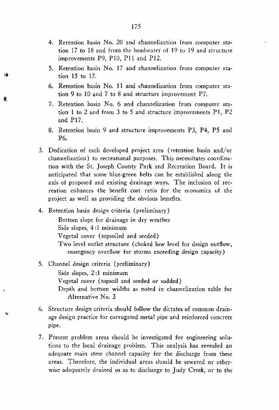
4. Retention basin No. 20 and channelization from computer sta­tion 17 to 18 and from the headwater of 19 to 19 and structure improvements P9, P10, P l l and P I2.

5. Retention basin No. 17 and channelization from computer sta­tion 15 to 17.

6 . Retention basin No. 11 and channelization from computer sta­tion 9 to 10 and 7 to 8 and structure improvement P7.

7. Retention basin No. 6 and channelization from computer sta­tion 1 to 2 and from 3 to 5 and structure improvements P I, P2 and P I 7.

8 . Retention basin 9 and structure improvements P3, P4, P5 and P 6 .

3. Dedication of each developed project area (retention basin and/or channelization) to recreational purposes. This necessitates coordina­tion with the St. Joseph County Park and Recreation Board. I t is anticipated that some blue-green belts can be established along the axis of proposed and existing drainage ways. The inclusion of rec­reation enhances the benefit cost ratio for the economics of the project as well as providing the obvious benefits.

4. Retention basin design criteria (preliminary)Bottom slope for drainage in dry weatherSide slopes, 4:1 minimumVegetal cover (topsoiled and seeded)Two level outlet structure (choked low level for design outflow,

emergency overflow for storms exceeding design capacity)

5. Channel design criteria (preliminary)Side slopes, 2:1 minimumVegetal cover (topsoil and seeded or sodded)Depth and bottom widths as noted in channelization table for

Alternative No. 3

6 . Structure design criteria should follow the dictates of common drain­age design practice for corrugated metal pipe and reinforced concrete pipe.

7. Present problem areas should be investigated for engineering solu­tions to the local drainage problem. This analysis has revealed an adequate main stem channel capacity for the discharge from these areas. Therefore, the individual areas should be sewered or other­wise adequately drained so as to discharge to Judy Creek, or to the

176

closest developed tributary to Judy Creek as outlined in Alternative No. 3.

8. This hydrologic data collection program should be continued for collection and analysis of significant hydrologic data for the basin.

SUM M ARY

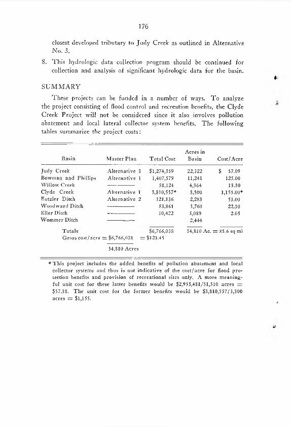
These projects can be funded in a number of ways. To analyze the project consisting of flood control and recreation benefits, the Clyde Creek Project will not be considered since it also involves pollution abatement and local lateral collector system benefits. The following tables summarize the project costs:

Basin Master Plan Total CostAcres in

Basin Cost/Acre

Judy Creek Alternative 3 $1,274,359 22,322 $ 57.09Bowman and Phillips Alternative 1 1,407,579 11,248 125.00Willow Creek 58,124 4,364 13.30Clyde Creek Alternative 1 3,810,557* 3,300 1,155.00*Eutzler Ditch Alternative 2 121,136 2,283 53.00Woodward Ditch 83,861 3,760 22.30Eller Ditch 10,422 5,089 2.05Wommer Ditch 2,444

Totals $6,766,038 54,810 Ac. = 85.6 sq miGross cost/acre = $6,766,038

54,810 Acre;=

$123.45

* This project includes the added benefits of pollution abatement and local collector systems and thus is not indicative of the cost/acre for flood pro­tection benefits and provision of recreational sites only. A more meaning­ful unit cost for these latter benefits would be $2,955,481/51,510 acres $57.38. The unit cost for the former benefits would be $3,810,557/3,300 acres rr $1,155.