Embed Size (px)
Citation preview

Assessment of Mercury in Waters, Sediments, and Biota of VT and NH Lakes Project. Draft Final Report. Page 1
Biogeochemistry of Mercury in Vermont and New Hampshire Lakes
An Assessment of Mercury in Water, Sediment and Biota of Vermont and New Hampshire Lakes
Comprehensive Final Project Report May, 2004
Project Funding Provided by United States Environmental Protection Agency
Office of Research and Development
under the
Regional Environmental Monitoring and Assessment Program
Cooperative Agreement Number CR-82549501
Investigators:
Neil Kamman Vermont Department of Environmental Conservation
103 S Main 10N Waterbury VT 05671-0408
802 241-3795
Dr. Charles T. Driscoll Syracuse University
Dep’t Civil and Environmental Engineering
Bob Estabrook Biology Bureau
NH Department of Environmental Services
Dr. David C. Evers Biodiversity Research
Institute, Falmouth ME
Dr. Eric. K. Miller Ecosystems Research
Inc., Norwich, VT
Assessment of Mercury in Waters, Sediments, and Biota of VT and NH Lakes Project. Draft Final Report. Page 2
t
Table of Contents
Table of Contents......................................................................................................................................... 2 List of Tables ............................................................................................................................................... 4 List of Figures .............................................................................................................................................. 5 Executive summary and recommendations ................................................................................................ 7 1.0 Introduction and acknowledgements..................................................................................................... 9 2.0 Project description, working hypotheses, and objectives ..................................................................... 11
2.1 General overview and experimental design ....................................................................................... 11 3.0 Site selection and sampling procedures ................................................................................................14
3.1 Sampling site selection ......................................................................................................................14 3.2 Site description and timing of collection...........................................................................................14 3.3 Sampling procedures .........................................................................................................................14 3.4 Sample custody..................................................................................................................................18 3.5 Field protocols ...................................................................................................................................19
4.0 Analytical procedures and calibration.................................................................................................. 23 5.0 Statistical approach to data analysis..................................................................................................... 25 6.0 Lakes sampled and data results ........................................................................................................... 27
6.1 Study lakes ........................................................................................................................................ 27 6.2 Water chemistry for core sampling lakes.......................................................................................... 32 6.3 Multiprobe profiles – core and paleolimnology lakes ...................................................................... 33 6.4 Sediment chemistry – core lakes ...................................................................................................... 34 6.5 Biological tissue chemistry............................................................................................................... 35 6.6 Paleolimnology of Hg in Vermont and New Hampshire lakes ....................................................... 36
7.0 Quality assurance and control resul s .................................................................................................. 40 7.1 Water chemistry parameters ............................................................................................................. 40 7.2 Solid phase parameters..................................................................................................................... 40 7.3 Laboratory intercomparison for HgT................................................................................................41 7.4 Problems........................................................................................................................................... 42
8.0 Analysis of the project data .................................................................................................................. 43 8.1 Calculation of age-adjusted yellow perch fillet HgT means for each study lake ............................. 43 8.2 GIS analyses...................................................................................................................................... 44 8.3 Statistical evaluation of strata in the experimental design ............................................................... 46 8.4 Cumulative frequency distribution diagrams................................................................................... 46 8.5 Evaluation of inter-annual variability and replicate sampling ......................................................... 49

8.6 Evaluation of Hg variation in relation to trophic status....................................................................51 8.7 Calculation of Hg bioconcentration and bioaccumulation factors .................................................. 53 8.8 Relationships among variables – univariate correlations ................................................................. 53 8.9 Principal components analysis - accounting for covariance among parameters ............................. 54 8.10 The influence of land-use on Hg .................................................................................................... 57 8.11 Development of candidate linear discriminant functions to predict tissue Hg levels in fillets given physicochemical data............................................................................................................................. 59 8.12 Summary of statistical analyses ...................................................................................................... 62
9.0 Estimation and mapping of atmospheric Hg deposition .................................................................... 64 9.1 Summary ........................................................................................................................................... 64 9.2 Concentrations of Hg species in the atmosphere ............................................................................ 64 9.3 Atmosphere-land surface transfers of Hg......................................................................................... 68 9.4 Tabulation of deposition results for the REMAP Lake-Watersheds............................................... 72 9.5 Discussion ........................................................................................................................................ 72 9.6 Deposition maps............................................................................................................................... 77 9.7 Relationship of deposition to in-lake Hg measures ......................................................................... 79
10.0 Data Archive ....................................................................................................................................... 79 11.0 References ........................................................................................................................................... 80 Appendix A. Historical and present fluxes of mercury to Vermont and New Hampshire lakes inferredfrom
t
i
i
210Pb dated sedimen cores ................................................................................................................ 86 Appendix B: Statistical Models of Atmospher c Hg Concentrations ....................................................... 87 Appendix C: Overview of the High Resolut on Deposition Model .......................................................... 89
Assessment of Mercury in Waters, Sediments, and Biota of VT and NH Lakes Project. Draft Final Report. Page 3

List of Tables Table 2.1. Breakdown of number of lakes by strata and state. ......................................................................................................12 Table 3.1. Referenced field sampling methods for water...................................................................................................................15 Table 4.1. Parameter table of referenced analytical procedures.........................................................................................................24 Table 5.0. Quality control sample frequency..................................................................................................................................25 Table 6.1. Roster of 103 lakes sampled.........................................................................................................................................28 Table 6.2. Summary of water chemistry data. ................................................................................................................................32 Table 6.3. Summary of multiprobe profile metadata.......................................................................................................................33 Table 6.4. Summary of sediment chemistry data.............................................................................................................................34 Table 6.5 Summary of biological tissue data. .................................................................................................................................35 Table 6.7.1. Diagnostic 210Pb dating values for 13 lakes. ...........................................................................................................37 Table 6.7.2. Modern, peak, and background Hg fluxes to the sediments of 13 lakes. ...................................................................38 Table 7.1. Quality assurance and control indicators for aqueous-phase parameters. .........................................................................40 Table 7.2. Quality assurance and control indicators for sediment-phase parameters. ........................................................................41 Table 7.3. Results of 10 laboratory intercomparison aqueous HgT samples....................................................................................41 Table 8.3. Results of ANOVA and ANOVA on Ranks tests of the influence of four lake:watershed area classes on multiple Hg parameters measured from 92 REMAP study lakes. ....................................................................................................................46 Table 8.5. Results of MANOVA and follow-up ANOVA analyses of inter-annual variability and replicate sampling...............49 Table 8.7. Log bioconcentration and bioaccumulation factors for biological Hg parameters in relation to aqueous Hg parameters. ...53
Table 8.8. Summary of significant (p≤0.05) Spearman correlation coefficients among water chemistry variables in relation to Hg parameters .....................................................................................................................................................................................54 Table 8.9.1. Results of principal components analyses for epilimnetic and hypolimnetic water chemistry datasets. .............................55 Table 8.9.2. Pearson correlation coefficients between principal components and measures of Hg in waters, sediments and biota.........56 Table 8.10. Spearman correlations between epilimnetic and sediment Hg parameters, and simplified land-use categories. .................58 Table 9.2.1.1. Mercury monitoring stations used to interpolate regional atmospheric mercury concentration fields............................65 Table 9.2.1.2. Seasonal precipitation-weighted average concentrations for the Hg monitoring sites. Values for the UMAQL protocol sites were adjusted to an MDN basis (equation 3). Concentrations are reported in ng l-1...................................................66 Table 9.3.4. Characteristics of regional forest types used in the dry deposition and litter fall Hg accumulation models. Leaf biomass estimates are from the forest survey conducted by Miller et al. (in preparation). ................................................................................72 Table 9.7. Spearman correlation matrix between atmospheric Hg deposition estimates, and in-lake Hg measures............................79
Assessment of Mercury in Waters, Sediments, and Biota of VT and NH Lakes Project. Draft Final Report. Page 4
List of Figures Figure 6.1. Geographic location of lakes sampled………………………………………………..……………………..27
Figure 6.6 Mercury risk to breeding Common Loons (Gavia immer), based on adult and juvenile blood and egg Hg levels……………………………………………………………………………………………………………………….36
Figure 6.7. 210Pb-inferred Hg fluxes to the sediments of 13 VT and NH lakes………….…………………………….39
Figure 8.1. Relationship between age and length-adjusted yellow perch muscle-tissue least squared mean Hg concentrations…………………………………………………………………………………………………………….43
Figure 8.2. Mercury in sediment, waters, and yellow perch tissues……………………………………………………45
Figure 8.4.1. Cumulative frequency distributions for Hg parameters measured in VT and NH lakes………………47
Figure 8.4.2. Cumulative frequency distributions for Hg parameters measured in VT and NH lakes…………...…47
Figure 8.5.1. Tukey box-plots of epilimnetic HgT concentration by year and state, for samples collected during 1998, 1999, and 2000…………………………………………………………………………...…………………………..50
Figure 8.5.2. Mean concentrations of HgT in epilimnetic waters (and 95% confidence intervals) by year and State………………………………………………………………………………………………………………………..50
Figure 8.5.3. 1991-2001 mean June through September precipitation at Burlington, VT and Concord, N.H……….51
Figure 8.6. Back-transformed least-squares means and 95% confidence intervals for four mercury parameters in relation to four lake trophic states……………………………………………………………………………………….52
Figure 8.9. Partial scatterplot matrix of several Hg parameters in relation to epilimnetic and hypolimnetic principal components of 11 water chemistry variables…………………………………………………………………………….57
Figure 8.11. Means and standard deviations for HgT in fillets of three species of freshwater fish from Maine lakes, in relation to the EPA 0.3 µg g-1 tissue Hg criterion……………………………………………………………………61
Figure 9.2. Estimated Hg concentration (ng l-1) field for summer precipitation……………………………………..67
Figure 9.3.4. Growing season Hg accumulation in foliage………………….. ……………………………………….71
Figure 9.5.1. Ratio of modeled “throughfall” (see text) to modeled precipitation flux of Hg……………………….73
Figure 9.5.2. Frequency distributions of modeled RGM flux (µg m-2 y-1)…………………………………………….73
Figure 9.5.3. Frequency distributions of modeled Hg fluxes (µg m-2 y-1) via litterfall………………………….……73
Figure 9.5.4. Frequency distributions of the total and component Hg fluxes to the REMAP study watersheds..…74
Figure 9.5.5. Frequency distributions of precipitation Hg flux to the REMAP study watersheds by season…...….75
Figure 9.5.6. Frequency distributions of particulate-phase Hg flux to the REMAP study watersheds by season…75
Figure 9.5.7. Frequency distributions of RGM Hg flux……………………………………………………………..…76
Figure 9.5.8. Frequency distributions of Hg0 flux to the REMAP study watersheds by season…………………….76
Figure 10.0. Data tables and structure for all information collected…………………………..…………………….…79
Assessment of Mercury in Waters, Sediments, and Biota of VT and NH Lakes Project. Draft Final Report. Page 5
The following document was prepared by the Vermont Department of Environmental Conservation, under a cooperative agreement with the United States Environmental Protection Agency, Office of Research and
Development. This report is submitted in fulfillment of obligations under cooperative agreement CR 825495-01. The information and data expressed herein do not necessarily represent the views of the VT Department of
Environmental Conservation, nor of the US Environmental Protection Agency. This document has not been subject to policy review by the US Environmental Protection Agency, and accordingly, the views expressed herein are
neither statements of USEPA policy nor of USEPA policy intent.
The Vermont Department of Environmental Conservation is an equal opportunity agency and offers all persons the benefits of participating in each of its programs and competing in all areas of employment regardless of race, color,
religion, sex, national origin, age, disability, sexual preference, or other non-merit factors.
This document is available upon request in large print, braille or audio cassette.
VT Relay Service for the Hearing Impaired 1-800-253-0191 TDD>Voice - 1-800-253-0195 Voice>TDD
Assessment of Mercury in Waters, Sediments, and Biota of VT and NH Lakes Project. Draft Final Report. Page 6
Executive summary and recommendations This report summarizes findings of a three-year field study of mercury in freshwater lakes of Vermont and New Hampshire. The study was undertaken jointly by the Vermont Department of Environmental Conservation, New Hampshire Department of Environmental Services, and Syracuse University. Collaborating organizations included the Biodiversity Research Institute, Dartmouth College, the Ecosystems Research Group, the Science Museum of Minnesota, the United States Fish and Wildlife Service, and the Vermont Department of Fish and Wildlife. Project funding and guidance were provided by the United States Environmental Protection Agency, under a cooperative agreement with the EPA Office of Research and Development. The study was initiated in 1998. Field sampling was completed at the close of the 2000 field season. Data analysis and modeling exercises were conducted during the period 2001-2002. The study was designed specifically to determine the generalized level of mercury contamination in sediment, water, and biota of multiple trophic levels across the VT-NH region, using a geographically randomized approach. This type of approach ensures that results provide a statistically valid representation of regionwide conditions. In this summary, average mercury concentrations are provided for several types of measurements, along with the 95% confidence intervals. Results of data analyses are highlighted, and interpretations that carry significant management implications are discussed. Measured values are discussed in light of currently available guidelines or water quality criteria. Mercury was detectable in waters of all lakes sampled. The average water-column total mercury (Hg) concentrations were 1.78 (± 0.1) parts-per-trillion (ppt) for shallow-water samples, and 11.52 (± 0.81) ppt in deep lake waters. Maximum total Hg concentrations were 9.44 and 33.41 ppt for the shallow and deep waters, respectively. Water methylmercury (meHg) showed a similar pattern of increase with depth. MeHg averaged 0.299 (± 0.018) ppt in shallow waters, and 0.829 (± 0.092) ppt in deep waters. The maximum concentrations were 3.12 and 4.45 ppt, for shallow and deep waters, respectively. The higher deepwater total Hg and meHg concentrations suggest accumulation in bottom waters, either due to loss from upper waters by sedimentation, release from deepwater sediments, or a combination of both. The average Hg concentration in sediments was 0.240 (± 0.01) parts per million (ppm); this agrees well with previous studies. Sediment methylmercury (meHg) averaged 1.7% (± 0.1%) of the sediment total Hg. Sediment Hg concentrations were highest in lakes occupying the most remote and forested regions of VT and NH, and were lowest in lakes with the greatest levels of watershed development. The historical deposition of Hg to the study region was reconstructed using paleolimnological techniques. Hg presently accumulates in lake sediments at a rate 3.7 times that of the period 1825 and before. In all lakes, a consistent increase in Hg accumulation was evident by the year 1850. The rate of sediment Hg accumulation is presently declining regionwide, and the onset of this decline is generally coincident with implementation of the 1990 Clean Air Act Amendments. The paleolimnological analysis also indicated that net atmospheric deposition to lakes across VT and NH is 21 µg m-2 yr-1. This estimate is consistent with direct measurements made at the Underhill, VT Hg deposition monitoring site. The paleolimnological analysis further indicated that a lag can be expected between reductions in emissions of Hg, and reductions in Hg accumulation to lake sediments, owing to Hg which is presently accumulated in watershed soils. The duration of this lag is unquantified at present, pending further study. This study also evaluated the accumulation of Hg in the tissues of lake fish and wildlife. Yellow perch (Perca flavescens) is a ubiquitous lake fish that is increasingly used to indicate of the strength of Hg bioaccumulation in lakes. In the present study, two size classes of perch were analyzed for Hg. Small perch were processed as composites of entire fish to assess the level of contamination available to piscivorous wildlife. Larger perch were processed as fillets of individual fish to assess the level of contamination relevant to human consumption. Methylmercury was analyzed in a subset of perch tissues to determine the overall proportion of methylated Hg in the fish. Common loons (Gavia immer) are a threatened, obligate fish-eating bird, known to be sensitive to mercury contamination. Loon tissues were analyzed for Hg from those study lakes where loons were present, as an
Assessment of Mercury in Waters, Sediments, and Biota of VT and NH Lakes Project. Draft Final Report. Page 7
indicator of potential impact on this species. Fillets of yellow perch averaged 0.239 (± 0.007) ppm, and ranged from a low of 0.051 ppm to a maximum of 1.3 ppm, which is quite elevated for yellow perch. Nearly 100% of the Hg in perch tissues was in the meHg form. Yellow perch fillets from NH lakes were significantly higher in Hg than were fish from Vermont lakes. Results of the loon tissue analyses suggested that across the region, 50% of Vermont lakes and 70% of NH lakes had loons with tissue Hg concentrations that placed those animals in a “moderate” or higher risk category. These perch and loon tissue data indicated that Hg contamination is readily bioaccumulated in most lakes across the VT-NH region. Further statistical analyses indicated that total and methyl-Hg derived from watersheds are more likely to be the main Hg source to fish and other biological tissues than are Hg and meHg derived from lake sediments. The roles of watershed land-use and lake trophic state were evaluated in relation to perch tissue Hg burdens. Perch muscle tissue Hg levels were positively correlated with increases in forested land use, and negatively correlated with increases in developed watershed area. Importantly, while both eutrophic (e.g., high algal density) and dystrophic (e.g., light-limited due to tannic acid content) lakes had similarly elevated levels of water Hg and meHg relative to other study lakes, only the dystrophic lakes showed significant bioaccumulation in yellow perch. The eutrophic lakes displayed very low levels of tissue Hg contamination. This finding suggests that fish tissues of biologically-productive lakes may be far lower in Hg than is currently presumed by existing fish tissue advisories. Various criteria exist for Hg to protect human health and aquatic life. The most conservative legal water quality criterion for mercury in VT waters is 12 ppt, to protect aquatic biota subject to chronic, low-level Hg exposure. The most conservative standard in NH is 51 ppt, to protect against bioaccumulation of Hg in gamefish. The National Oceanic and Atmospheric Administration has a long-standing sediment quality guideline for Hg of 0.15 ppm, above which a “low” or greater risk of impact to sediment-based biota is likely. The method employed by the VT Department of Health to set tissue advisories, based on ‘normal’ fish consumption patterns, yields a maximum tissue Hg concentration of approximately 0.2 ppm. Above this value, limited fish consumption is advised for some portion of the population. EPA has recently promulgated a similarly-derived, tissue-based criterion of 0.3 ppm meHg as a safe maximum fish-tissue concentration. The present study provides an opportunity to evaluate these criteria and risk assessment concentration thresholds in light of VT and NH specific data. In this study, no shallow lake waters violated the Vermont water column criterion, and only 16% of lakes across the region showed violations in the deep water portions of the lakes. No lakes exceeded the NH water column criterion. However, fish tissue contamination in excess of criteria limits was found in many lakes and most lake types. Thirty percent of lakes sampled had perch fillet means in excess of the USEPA criterion, and 60% of lakes had perch fillet tissues exceeding 0.2 ppm. Ninety percent of lakes displayed sediment Hg concentrations in excess of the National Oceanic and Atmospheric Administration sediment quality guideline. These findings clearly indicate that the existing numeric water column criteria within the VT and NH standards are not sufficiently conservative to limit accumulation of Hg to sediments, or to limit risks to humans due to fish consumption, and to limit risks to the wildlife. A statistical model was developed to predict the likelihood that tissue meHg concentrations of yellow perch would exceed the USEPA meHg criterion, using data from the study lakes. This model uses simple measures of water chemistry (lake buffering capacity, conductance, acidity, organic content, flushing rate) and is applicable to VT and NH lakes 20 acres in size or larger. Based on the model results, 29% of all VT lakes and 62% of all NH lakes are likely to violate the USEPA criterion. This model can be used as a screening tool to identify lakes in need of additional fish tissue sampling in the Vermont-New Hampshire region, and can serve as a general guide identifying those parameters that are most important in controlling fish-tissue Hg concentrations in other regions of north America. One additional component of this study estimated Hg deposition to the VT-NH region based on a sophisticated, high-resolution and geographically-based deposition model. This analysis showed that dry deposition of Hg can
Assessment of Mercury in Waters, Sediments, and Biota of VT and NH Lakes Project. Draft Final Report. Page 8
equal or exceed that deposited in precipitation, and is enhanced in the higher elevations of the VT-NH region. Specifically, maps of deposition by type (e.g., precipitation, particulate, Hg vapor) indicate that dry deposition is most greatest over higher-elevation, forested terrain. Wet Hg deposition showed regional patterns, with greater deposition in southern VT, southeastern NH, and along the mountain chains of both states. Overall deposition estimates were in good agreement with those derived using paleolimnological techniques. The deposition estimates were also assessed in relation to in-lake measures of Hg contamination. Both shallow-water meHg and prey-sized yellow perch Hg burdens were elevated in lakes where wet Hg deposition was also elevated. There were no significant relationships between estimates of dry Hg deposition and in-lake Hg measurements. With respect to management recommendations, the following merit consideration:
1) Sufficient data are available within this project dataset to develop a TMDL for Hg for lakes in either VT or NH. USEPA Region 1 is presently deliberating on the applicability of individualized TMDLs for lakes, and is considering as an alternative a modeling analysis to support a New England-wide regional TMDL for Hg. While a regional TMDL seems most applicable to the type of threat posed by Hg, should VT or NH be required to develop waterbody or state-specific TMDLs the integrated dataset presented herein will provide a sound basis for the analysis. The data from this project can also support a regional TMDL approach.
2) The existing water column criteria for Hg in Vermont and New Hampshire are not sufficiently
conservative to protect human health and aquatic biota. These criteria should be revised during each states water quality standards review. Consideration should be given to the EPA criterion for meHg in fish tissue and also to ongoing research by the Biodiversity Research Institute to develop criterion values protective of piscivorous wildlife.
3) Our findings regarding trophic status and pH mediation of Hg bioaccumulation should be used to guide
further fish tissue collection efforts for the refinement of consumption advisories. Specifically, additional eutrophic lakes should be sampled for fish tissue Hg to identify waters where advisories may be relaxed. The statistical model derived for this study can also be used to identify previously untested lakes where additional fish-tissue sampling is warranted.
4) The dataset generated by this study serves as a baseline assessment of Hg across the VT-NH region, for
the period 1998-2000. Several federal initiatives are presently under consideration for controlling Hg emissions, and numerous states have already reduced both emission sources and the rate of disposal of Hg-bearing products. Accordingly, the level of Hg contamination of the northeastern landscape is expected to decline over the next decade or more. One or more components of this project, re-executed after a ten-year or longer time period has passed, would provide insight into the success of these initiatives.
1.0 Introduction and acknowledgements Beginning in spring of 1998, the Vermont Department of Environmental Conservation (VTDEC), in cooperation with the New Hampshire Department of Environmental Services, Syracuse University, USEPA, and several other collaborators, launched an effort to measure the level of mercury (Hg) contamination in lakes and lake biota across Vermont and New Hampshire. Over the course of the 1998 through 2000 field seasons, we conducted an intensive field measurement program on 103 lakes and ponds. On the vast majority of these lakes and reservoirs, water and sediment chemistry parameters including total mercury (HgT), and methylmercury (meHg), were collected. On a subset of the waterbodies, HgT (and in some cases meHg) was also measured in macrozooplankton, prey-sized and human-consumption sized yellow perch, and in avian obligate piscivores such as common loons, mergansers, and belted kingfishers. On a smaller subset of lakes, the rate of historical Hg deposition of Hg to lake sediments was estimated using paleolimnological techniques. Estimates of atmospheric Hg deposition, derived by a project collaborator using data from the parallel “NESCAUM-EPA Region 1”
Assessment of Mercury in Waters, Sediments, and Biota of VT and NH Lakes Project. Draft Final Report. Page 9
companion REMAP project and other sources, were made for wet, dry, and particulate Hg deposition to the VT-NH region. These estimates were derived using a big-leaf modeling approach, and are reported herein. The goal of this project was to determine which large, publicly-used Vermont and New Hampshire lakes are of the type that: 1) have excessive mercury in their sediments and waters; 2) possess conditions linked to converting this mercury into toxic meHg; and 3) have high mercury concentrations in plankton, fish, and fish-eating wildlife. The results of this study have already been used in part to refine Hg fish-tissue consumption advisories in Vermont and New Hampshire, and also to learn more about factors influencing bioaccumulation of mercury in freshwater biota. Our final results provide baseline chemical and biological indicators of Hg contamination, against which future reductions of atmospherically emitted mercury can be measured. This study provides a large integrated dataset that compliments similar datasets in the State of Maine, and in the Adirondack region of New York. The present dataset is unique in the level of integration between measurements of Hg in multiple physical and trophic ecosystem compartments. Collaborators on the project included Celia Chen (Dartmouth College), Dan Engstrom (Science Museum of Minnesota), Dave Evers (Biodiversity Research Institute of Freeport, Maine), Peter Lorey (Syracuse University), Drew Major (US Fish and Wildlife Service New England Region), Bernie Pientka (Vermont Department of Fish and Wildlife), and Rob Taylor (Texas A&M). This report was written by Neil Kamman, and Section 9 and Appendices 1-3 were provided by Eric Miller. We gratefully acknowledge project funding from USEPA-ORD under cooperative agreement CR-82549501. We also acknowledge the eager participation of the following individuals, without whom it would have been impossible to execute this project: Mr. Wing Goodale and Ms. Oksana Lane of the Biodiversity Research Institute, for their work capturing loons and kingfishers; Mr. Steve Couture, Mr. Steve Landry, and Ms. Elizabeth Roy of the NH Department of Environmental Services, for their countless hours of field work and logistical support in NH waters; Ms. Kelly Thommes of the Science Museum of MN, for her work dating sediment cores; Mr. Tim Gleason of the USFWS, for hours of patient fishing for yellow perch; Dr. Rochelle Araujo, Mr. Ray Thompson, and Mr. Alan VanArsdale of USEPA for their steadfast and long-term support of the project; and finally, Mr. Ed Glassford, who analyzed hundreds of sediment samples for the project. The team also wishes to acknowledge the major contribution to the project provided by Ms. Kate Peyerl of VTDEC, who coordinated all VT sampling events, processed countless sediment and fish tissue samples, entered hundreds of lines of data, and handled myriad logistical details.
Assessment of Mercury in Waters, Sediments, and Biota of VT and NH Lakes Project. Draft Final Report. Page 10

2.0 Project description, working hypotheses, and objectives 2.1 General overview and experimental design The purpose of this research was to characterize concentrations of HgT and meHg in waters and sediments of Vermont and New Hampshire lakes, and to relate these data to easily measured water column chemical parameters and watershed-level physical attributes. A primary research goal was to identify specific lake types in which elevated levels of methylmercury are formed, and in which this toxic for of mercury is accumulated into middle and higher trophic-level organisms. The general design of this comparative observational study follows. The project was conducted as a three-year, stratified, spatially randomized sampling employing the EPA Environmental Monitoring and Assessment Program (EMAP) Surface Waters experimental approach. In this approach, sampling units were selected by Geographic Information System, using the hexagon algorithm to ensure random identification of sampling units given the constraints of any stratification (blocking) imposed on the selection. In this study, individual lakes were considered sampling units. We evaluated two size-strata of lakes that were greater than 20 acres in size. These two size-strata were further grouped according to their watershed to lake area ratios, since this ratio has been shown to influence total aqueous mercury levels in water (Mierle and Ingram, 1991). Individual selected lakes were assigned weights, proportional to the number of geographically proximal lakes represented by the selected lake within each hexagon. Using these weights, it is possible to estimate the overall level of Hg contamination for the entire population of waters represented by each sample. A second group of lakes was sampled to estimate historic fluxes of Hg to lake sediments. The selection of study lakes was as follows: 1) REMAP Core Sampling Lakes 1a) VT and NH lakes of 20 to <100 acres in size. These lakes were further grouped into two sub-strata,
based upon their lake:watershed area ratio. 1b) VT and NH lakes, 100 or more acres in size. These lakes were further grouped into two sub-strata, based
upon their lake:watershed area ratio.
- The EMAP spatially randomized selection protocol identified in excess of 90 lakes, representing approximately 11 percent of the total number of lakes of 20 acres in size or greater within the two States as candidates for sampling. Additional lakes were also selected as ‘overdraw’ lakes. The number of lakes within each strata, and by State, is listed in Table 2.1, and the final roster of lakes sampled is provided in Section 6.
2) Paleolimnology Lakes Thirteen such lakes were sampled. The selection process for these lakes was not random. Nine forested, so-called pristine lakes of a range of lake:watershed-area ratios were selected. Four additional lakes in developed or agricultural watersheds were also sampled. For groups 1a and 1b, lakes were visited once, and surficial sediment samples for HgT and meHg acquired from a single, representive sampling station. Water samples for HgT and meHg were procured from the epi- and hypolimnion of the overlying water column, using strict mercury-clean collection protocols. Major solutes and parameters related to meHg formation were measured from the overlying water column using standard limnological collection protocols and a multiparameter automated sonde. Details regarding sampling and analytical methods are given in sections 3.0 and 4.0 respectively. For group two, sediment HgT and 210Pb were measured. Fluxes of HgT to sediments were estimated as the product of sedimentation rate and HgT concentration for each sediment core layer.
Assessment of Mercury in Waters, Sediments, and Biota of VT and NH Lakes Project. Draft Final Report. Page 11
Field operations were conducted by the VTDEC - Water Quality Division, and NHDES - Biology Bureau. Chemical analyses of sediments, fish tissue, and most water samples were performed at the VTDEC LaRosa Environmental Laboratory. Dr. C.T. Driscoll (Syracuse University, Department of Civil, Environmental and Chemical Engineering) oversaw sediment meHg and aqueous HgT and meHg analyses, and participated in the analysis of the project data. Preyfish and piscivore Hg and meHg analyses were performed by Dr. Rob Taylor at Texas A&M University. A rigorous program of quality assurance and quality control was applied to both the field and laboratory phases of this project.
2.2 Project hypotheses and statement of project objectives
2.2.1 Hypotheses:
The concentrations of surficial sediment total mercury and aqueous total mercury in Vermont and New Hampshire lakes are related to physico-chemical lake and watershed characteristics.
VTDEC and NHDES's respective lakes and ponds databases contain physical and chemical data on approximately 810 lakes of 20 acres in size or greater. The databases include such physical information as elevation, lake size and morphometry, watershed size, and watershed area in wetlands, as well as multiple parameters related to lake trophic state and land use. In addition, a new geographically based land-use data set is available for Vermont and NH. It is hypothesized that sediment total mercury concentrations co-vary with one or more of these measurements.
Concentrations of sediment and aqueous methylmercury in Vermont and New Hampshire lakes are related to
sediment total mercury concentrations, and are mediated by lake and watershed level physical and chemical parameters.
It is hypothesized that sediment methylmercury and water column total and methylmercury concentrations covary with sediment mercury concentrations, and with water quality parameters such as major solutes, hypolimnetic sulfide, measures of dissolved organic carbon (DOC), and degree of hypolimnetic anoxia.
Sediment-mercury fluxes, evidenced in the stratigraphy of selected Vermont and New Hampshire lake sediment cores, show detectable variation over the past 300 years.
It is hypothesized that a rise above background sediment mercury concentrations and fluxes is detectable in 210Pb-dated short cores, the time signature of which corresponds to the industrialization of the United States. It is further hypothesized that detectable declines in both concentrations and fluxes are apparent in recently deposited sediments.
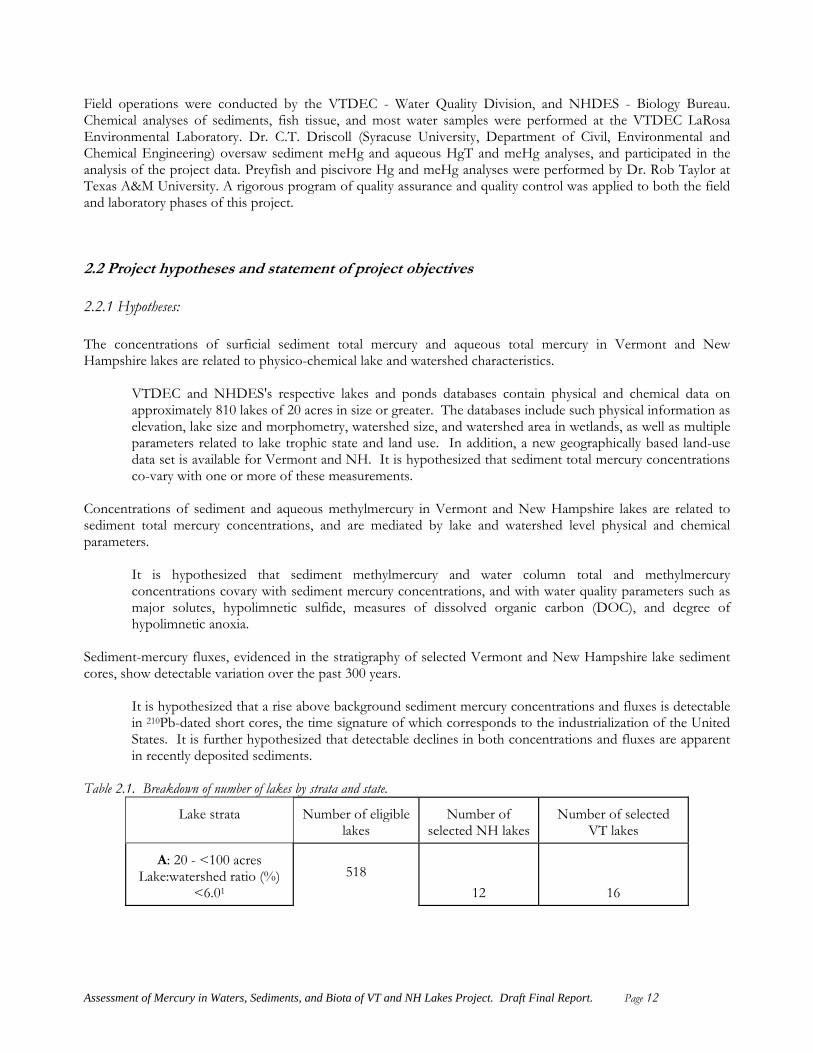
Table 2.1. Breakdown of number of lakes by strata and state.
Lake strata
Number of eligible
lakes
Number of
selected NH lakes
Number of selected
VT lakes
A: 20 - <100 acres Lake:watershed ratio (%)
<6.01
518
12
16
Assessment of Mercury in Waters, Sediments, and Biota of VT and NH Lakes Project. Draft Final Report. Page 12
Lake strata
Number of eligible
lakes
Number of
selected NH lakes
Number of selected
VT lakes
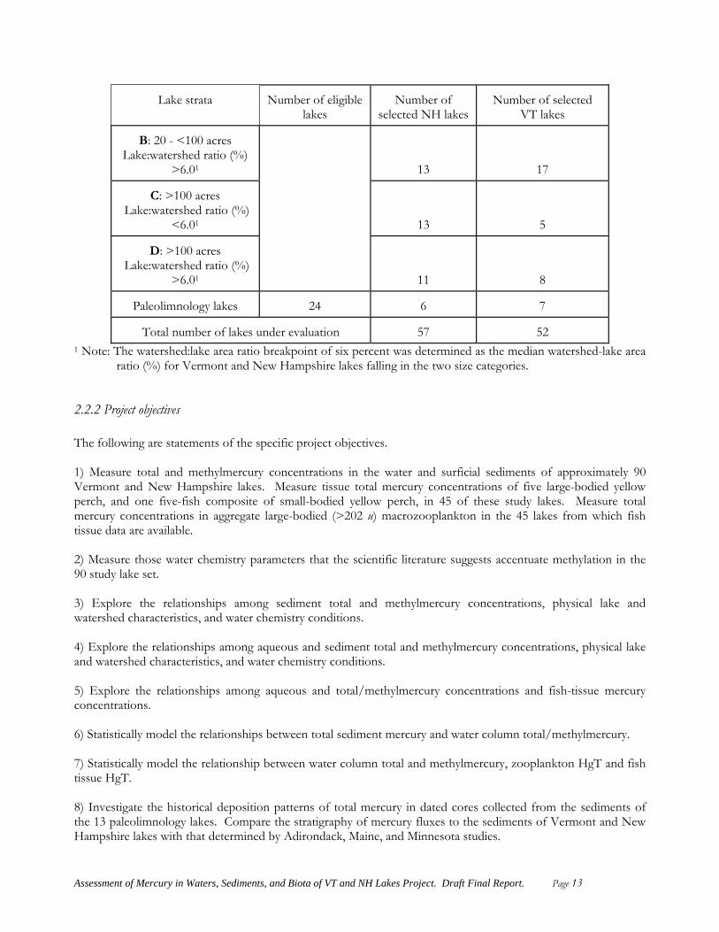
B: 20 - <100 acres Lake:watershed ratio (%)
>6.01
13
17
C: >100 acres Lake:watershed ratio (%)
<6.01 13
5
D: >100 acres
Lake:watershed ratio (%) >6.01
11
8
Paleolimnology lakes
24
6
7
Total number of lakes under evaluation
57
52
1 Note: The watershed:lake area ratio breakpoint of six percent was determined as the median watershed-lake area ratio (%) for Vermont and New Hampshire lakes falling in the two size categories.
2.2.2 Project objectives The following are statements of the specific project objectives. 1) Measure total and methylmercury concentrations in the water and surficial sediments of approximately 90 Vermont and New Hampshire lakes. Measure tissue total mercury concentrations of five large-bodied yellow perch, and one five-fish composite of small-bodied yellow perch, in 45 of these study lakes. Measure total mercury concentrations in aggregate large-bodied (>202 u) macrozooplankton in the 45 lakes from which fish tissue data are available. 2) Measure those water chemistry parameters that the scientific literature suggests accentuate methylation in the 90 study lake set. 3) Explore the relationships among sediment total and methylmercury concentrations, physical lake and watershed characteristics, and water chemistry conditions. 4) Explore the relationships among aqueous and sediment total and methylmercury concentrations, physical lake and watershed characteristics, and water chemistry conditions. 5) Explore the relationships among aqueous and total/methylmercury concentrations and fish-tissue mercury concentrations. 6) Statistically model the relationships between total sediment mercury and water column total/methylmercury. 7) Statistically model the relationship between water column total and methylmercury, zooplankton HgT and fish tissue HgT. 8) Investigate the historical deposition patterns of total mercury in dated cores collected from the sediments of the 13 paleolimnology lakes. Compare the stratigraphy of mercury fluxes to the sediments of Vermont and New Hampshire lakes with that determined by Adirondack, Maine, and Minnesota studies.
Assessment of Mercury in Waters, Sediments, and Biota of VT and NH Lakes Project. Draft Final Report. Page 13
3.0 Site selection and sampling procedu es r
f
3.1 Sampling site selection Individual study lakes were selected by the USEPA National Health and Environmental Effects Research Laboratory in Corvallis, OR, using the EMAP, stratified, spatially randomized lake selection process (USEPA 2002). In brief, this process employs a Geographic Information System (GIS) to overlay a hexagonal grid onto a base waterbody GIS datalayer. The mesh of the overlay grid is sized in proportion to the total number (population) of waterbodies from which the sample is drawn, and to the size of the geographic area under consideration. The computer system then assigns a series of randomly generated coordinates, which are scaled to fall within the coordinate-space of the overlay grid. The single lake waterbody nearest to each randomly-selected grid intersect is considered part of the sample. For this sample, lakes were selected from the USEPA Reachfile III waterbody base layer. Lakes were selected as described in Table 2.1. All Vermont and New Hampshire lakes of 20 acres in size or greater were considered ‘eligible’ for selection with the exception of the following:
1) Lakes Champlain, Memphremagog, Squam, and Winnipesaukee. The design of this monitoring effort is inadequate to characterize the very large and unique segments of these lakes.
2) Connecticut River Reservoirs. The configuration and hydrology of Connecticut River Reservoirs is such that they behave in a significantly different manner than other Vermont and New Hampshire lakes and reservoirs. While other reservoirs were eligible for selection as study lakes, the highly dynamic Connecticut River Reservoirs were excluded from the pool of potential study lakes.
3.2 Site description and timing o data collection The main sampling location for each lake was centrally-located over the lake’s 'deep-hole.’ Sediment and water column samples were collected from these stations. Two critical water quality parameters that mediate methylation, hydrogen sulfide and dissolved oxygen, are strongly controlled by thermal stratification. The optimal timing for sampling such lakes is during mid- to late summer, when stratification is maximized. All dimictic (or mono/meromictic) lakes that were known to stratify during the summer months were sampled between late July and mid-August. The sampling of smaller polymictic lakes was relegated to the edges of this period. All lakes were sampled between June 28 and September 15 of each sampling season. To address interannual variability, as well as to address quality assurance concerns, several lakes were sampled in more than one season. 3.3 Sampling procedures The sampling station was located in the field using GPS. On lakes where gasoline powered craft were required for sampling, the engine was shut off downwind of the station, and rowed into place. When necessary, the boat was secured by anchor, and adequate anchor scope let out to avoid contamination of the hypolimnetic zone of interest by the anchor or by sediment drift. For all lakes, collection of parameters requiring clean handling preceded sample collection for the other parameters in like matrices. The order of collection and handling was as follows: Arrange sampling equipment - Don sampling attire and gloves - Surface grab for aqueous methylmercury and total mercury sample - Hypolimnetic teflon Kemmerer grab for aqueous methylmercury and total mercury sample - Remove clean attire and gloves - Collect then handle samples for other water chemistry parameters using Kemmerer sampler - multiprobe profile and Secchi measurement - Dirty hands collects sediments - Clean hands handles extruded sediment for methylmercury and total mercury.
Assessment of Mercury in Waters, Sediments, and Biota of VT and NH Lakes Project. Draft Final Report. Page 14

3.3.1 Acquisition of water for Hg and meHg A surface grab for aqueous mercury samples was collected at each study lake. In addition, for those lakes that stratify strongly, a sample was acquired from one meter above the sediment water interface, using an all-teflon Kemmerer sampler, cleaned to Method 1669 specifications (USEPA 1996a). The sampling depth was determined by on-board SONAR. Techniques for the collection of aqueous mercury samples conformed to EPA method 1669 ‘clean hands-dirty hands’ techniques. Briefly, sampling staff wore clean and new Tyvek™ windsuits, and powder-free vinyl gloves. ‘Clean hands’ wore shoulder-length gloves, and, if necessary for the logistics of the collection, additional shorter gloves. Gloves were new from the box at the time they were put on. Aqueous mercury samples were stored in a separate, designated clean cooler. Samples were preserved in situ with 3.6ml concentrated, trace-metals grade HNO3 (Dr. C.T. Driscoll, pers. comm.), using a new pipette tip rinsed twice in mercury-clean 10% HCl, and once in trace metal grade HNO3. A detailed field protocol can be found in section 3.5.
3.3.2 Other water chemistry parameters Water column sampling procedures are referenced in Table 3.1. Water sample aliquots were decanted to appropriate laboratory sample containers in the field, and transported on ice to the Vermont Department of Environmental Conservation LaRosa Laboratory for analysis. Aliquots for dissolved-phase samples were filtered in the field using Gelman Sciences 0.45u filter membranes. Table 3.1. Referenced field sampling methods for water.
Parameter
Collection Method
Method
Reference1
Field Sample
Container
Sample Preservation
Alkalinity
250 ml HDPE
4oC,
Dissolved and Apparent Color
50 ml poly-
carbonate tube.
4oC
Dissolved Organic Carbon
50 ml poly-
carbonate tube.
4oC, filtered to 0.45u,
acidified with H2SO4 to pH < 2
Sulfate Chloride
50 ml poly-
carbonate tube.
4oC
NOx
250ml HDPE
4oC, H2SO4 to pH <2
Sulfide
Kemmerer grab
2.2.3
250 ml glass
4oC, Zn Acetate, NaOH
Mercury
Surface grab and all-
teflon Kemmerer grab (hypolimnion)
16692
1000ml teflon 500ml teflon
4oC 3.6ml conc. HNO3, double-bagged. Stored frozen after delivery to
Syracuse Temperature DO, field pH Conductivity
Multi-probe sonde (Hydrolab®), water
column profile
Hydrolab Minisonde Surveyor
IV Manual
in situ
N/A
Assessment of Mercury in Waters, Sediments, and Biota of VT and NH Lakes Project. Draft Final Report. Page 15

Parameter
Collection Method
Method
Reference1
Field Sample
Container
Sample Preservation
Water Transparency
Secchi disk observation
1.2.1
in situ
N/A
1)Field Methods Manual, Vermont Department of Environmental Conservation, 1990. 2)USEPA 1996a. Water column samples for all non-Hg parameters were collected in the epilimnion and hypolimnion of each lake that displayed thermal stratification, and in the epilimnion only for shallow, mixed lakes. For epilimnetic samples, a Kemmerer grab from the one-meter depth, and from one meter above the upper knee of the thermocline were composited. Hypolimnetic samples were collected at one meter above the sediment-water interface.
3.3.3 Acquisition of sediments for Hg analysis In designing this part of the sampling protocol, we polled research professionals with experience in the collection of sediments for mercury analysis for their suggestions. The sediment collection methods presented below were designed based upon the comments and recommendations of the following. Dr. J. Becker; Dr. R. Bindler; Mr. P. Garrison; Dr. M. Ostrofsky; Dr. B. Simmers; Dr. E.B. Swain; and Dr. C.J. Watras. Sediments were acquired using a Glew-design, modified KB corer with a 60 cm by 7 cm lexan core tube, or a KB corer with a 60 cm by 5cm lexan tube and a cellulose acetate butyrate liner (NH lakes in 1998 only). The use of core catchers with the KB corer was precluded due to their potential to contaminate surficial sediments during the coring operation. Prior to initiation of sampling, the core tubes were acid cleaned. The tubes were also rinsed copiously in lake water prior to use, and copiously re-rinsed in lake water after sediments were extruded. Core tubes were stored in doubled, plastic bags between collections. These storage bags were replaced regularly, and core tubes were re-acidwashed not less than after every core collected. In most cases, tubes were acidwashed after every fifth sample. Core sectioning tools (scraper, lexan sectioning tray) were cleaned following the same schedule as core tubes, and were also stored in plastic. We adapted the clean hands-dirty hands protocol when collecting and sectioning sediments, as described in detail in Section 3.5. 3.3.3.1 REMAP study lakes Two cores were taken at each sampling station, and the ‘best’ core reflecting the least disturbance was selected for analysis. The top five centimeters of sediment, by individual centimeter interval, was extruded onto a copiously-rinsed, clean lexan sectioning tray (Gilmour et al., 1992; EPRI, 1996), then transferred into a new, clean zip-style bag (1998), or PETE bottle (1999), using an acid-clean plastic scraper. Sediments were extruded by individual one-centimeter thickness intervals in order to maintain tight control over the depth of sediments that were analyzed for HgT and meHg concentrations. Sediments were stored double-bagged, in a specially designated cooler. At no time were sediment samples placed into the same cooler as aqueous mercury samples. Samples were kept dark at 4oC, and returned to the laboratory for analysis of HgT by CVAA. Sediment aliquots for MeHg analysis by CVAFS were frozen upon receipt at the Syracuse laboratory. Detailed analytical procedures are provided in Section 4 below. 3.3.3.2 Paleolimnology lakes Sediments were collected using either a KB™ (Wildlife Supply Corp., Buffalo, N.Y.) or Glew-design modified KB corer at the deep lake station. In the field, sediment subsamples (cookies) were extruded in one-centimeter thickness increments to the bottom of each core. In general, sediment cores collected with these gravity corers were approximately 50cm in depth.
Assessment of Mercury in Waters, Sediments, and Biota of VT and NH Lakes Project. Draft Final Report. Page 16
As described in the “Coring Procedure” (Section 3.5.3 following), two cores were acquired from the sampling station, and the core reflecting the least disturbance was selected for sectioning and analysis. The one-centimeter sediment ‘cookies’ were stored in lot-certified PETE 125 ml round bottles. HgT concentration and percent carbon as loss on ignition (LOI) was subsequently analyzed from sediment aliquots on the following cookies: 0-1, 1-2, 2-3, 3-4, 4-5, 5-6, 7-8, 10-11, 12-13, 15-16, 17-18, 20-21, 25-26, 30-31, 35-36 (additional cookies were acquired from each fifth centimeter interval as needed, to the core bottom). All sediment subsamples were analyzed for percent solid by gravimetric analysis, then ground by mortar and pestle for 210Pb/226Rn counting and dating.
3.3.4 Acquisition of fish tissue Fish were collected using fike and experimental net sets, by electroshocking, or by angling. This element of the project was conducted in NH by NHDES staff with assistance from the USFWS. In Vermont, fish were collected by VTDFW. Fish were doubly bagged in new ziplock bags, and frozen for subsequent analysis at the LaRosa laboratory. At least ten 10 yellow perch per lake were targeted from 45 lakes. Yellow perch were selected because the species has successfully been used in previous studies of fish-Hg uptake, and in the development of fish consumption advisories (Driscoll et al., 1994, VTDEC 1992 rev. 2001). In addition, yellow perch are ubiquitous in Vermont and New Hampshire (T. Hess, VT Department of Fish and Wildlife, Waterbury, Vermont, personal communication). Targeting this single fish species controls for problems associated with the differential abilities of varyous fish species to assimilate and depurate Hg. Fish were frozen until prepared for laboratory analyses as described in Section 4. The analyses were performed between December, 1999 and January, 2000. Each outer bag was accompanied by an identification label with the following information. 1. Identification number (lake_code - fish#). For example KENTP - 01 2. Date 3. Species 4. Length (cm) 5. Weight (grams)
3.3.5 Acquisition of zooplankton samples Bulk zooplankton in the ≥201 u size fraction were collected with specially designed nets fabricated of non-metal materials. The dimensions of these nets were 30 cm by 125 cm, ≥201 µ, equipped with a detachable 200ml ‘Dolphin’ reduction bucket (Wildlife Supply Company, Saginaw MI). All zooplankton collections were made between 7/18/2000 and 9/6/2000. More information is provided in the protocol for acquiring zooplankton for mercury analysis for the REMAP Assessment of Mercury in Vermont and New Hampshire Lakes Project (Section 3.5.3, following). In summary, a minimum of 5 net tows were collected from the immediate vicinity of each lakes sampling station, and the contents composited, reduced, and decanted to a pre-weighed, graduated 50ml sample vial, after which the total volume of the sample was constituted to 50ml. The length of each individual tow composited was recorded on the field sampling sheet. This composite sample was used to measure HgT in the plankton, as well as total planktonic biomass. The modified clean-hands dirty hands protocol used for this collection is described in detail in Section 3.5.
Assessment of Mercury in Waters, Sediments, and Biota of VT and NH Lakes Project. Draft Final Report. Page 17

3.3.6 Tissues samples from piscivores All sampling used nonlethal methods. Blood and feathers were collected from captured adult and juvenile loons. Loons were captured using nightlighting methods. The technique of using vocalizations and playback recordings to attract a loon is most effective for capturing parental adults. Once within reach, the loon is scooped with a large dip net into the boat. The captured bird is then measured, banded, and blood and feathers taken before release in its territory 20-40 minutes later. Eggs were opportunistically collected from abandoned nests. Second flight secondary feathers were used for Hg analysis, and were cut at a standardized location along the rachis and weighed on a digital scale. These procedures are described in detail by Evers et al. (2000). For blood samples, blood was drawn from the metatarsal vein through a leur adapter directly into 5-10 cc vacutainers with sodium heparin (green tops). The vacutainers were opened once 10-14 hours later to add 10% buffered formalin (1:20 formalin-blood ratio) from a sealed container with a new 1 cc syringe. Each vacutainer with blood preserved by formalin was then refrigerated and not opened again until reaching the lab. Feathers were clipped at the calamus and placed in a polyethylene bag. Whole eggs were frozen in a polyethylene bag after field removal. Frozen eggs were later cracked and the contents (including the inner shell membrane) placed in lot-certified I-Chem jars that were not opened until reaching the lab. All piscivore samples were labeled in the field using a standard protocol which includes date, species, age, sex, band number, lake and territory name, and state, and all samples were double labeled. A catalog accompanied the samples when they were sent to the analytical lab. 3.4 Sample custody
3.4.1 Sample handling and transport protocols, and labeling and tracking Since VTDEC and NHDES maintain their own small and efficient laboratory operations, chain-of-custody procedures typically required of regulatory samples were not employed in conjunction with field operations. Field personnel were personally responsible for the samples until they were logged into the LaRosa Environmental Laboratory. In the laboratory, samples were accessioned according to the LaRosa laboratory standard protocol. All samples sent to other laboratories were delivered via tracked Federal Express shipments.
3.4.2 Field forms A standard field form accompanied all samples collected in conjunction with this study. The field forms identified the study lake, station location from GPS, date and time of sampling, and sampling crew. In order to trace potential contamination problems, serial numbers for sampling equipment were also included on the field form, and tracked using sample field identification numbers. This information was entered into the project database as samples were submitted.
3.4.3 Field data entry In order to avoid potential transcription error and maximize efficiency, data entry was largely automated. Date, field data and other ancillary information was entered into the LaRosa Laboratory Management System at the time of sample log-in, and was available for automated download to the project database. The format of the Lab Management System log-in code for samples submitted follows: Standard REMAP samples: FieldId_Time_QA_SampleDepth_SeccDepth_Apparatus# Paleolimnological samples: FieldId_P_Time_CookieDepth_Apparatus#_Tube# For example:
Assessment of Mercury in Waters, Sediments, and Biota of VT and NH Lakes Project. Draft Final Report. Page 18

SILVL01_1200_A_16.5_03.4_VT-1 consisted of a regular sample from Silver Lake (Leicester, VT), collected at noon, using Kemmerer bottle VT-1, at 16.5 meters depth, with a corresponding Secchi transparency of 3.4 meters. SILVL01_P_1353_08.0_GL_01 consisted of a sediment sample from Silver Lake (Leicester, VT) from 8 centimeters downcore, collected at 1353 using the Glew corer and core tube 1. The following QA codes were valid for entry associated with field samples: A- regular sample; B-field blank; D-field duplicate. Multiprobe data were ported from the datalogger directly into the project database on a weekly or more frequent basis. 3.5 Field protocols Precise field protocols for sampling water, and sediment for HgT and meHg, and zooplankton, fish tissue, and piscivore tissue for HgT, are provided in the following:
3.5.1 Water samples for HgT and meHg Epilimnetic Grab Sampling • Waterproof sample labels are prepared using waterproof ink. • ‘Dirty hands’ opens the ‘clean box,’ gloves, and dons a tyvek suit. • ‘Dirty hands’ removes shoulder gloves, and assists ‘Clean hands’ in donning shoulder-gloves and shorter
gloves if necessary. From this point forward, ‘Clean hands’ handles nothing but the sample bottle, or the inner ziplock bag that contains the sample bottle.
• ‘Dirty hands’ opens the ‘clean cooler’ and removes one 1000ml double bagged bottle. ‘Dirty hands’ opens the outer bag.
• ‘Clean hands’ reaches into the outer bag, opens the inner bag, removes the bottle, and folds the inner bag over.
• ‘Dirty hands’ seals the outer bag, and replaces it into the ‘clean cooler.’ • ‘Dirty hands’ removes the autopipet from the clean cooler, and affixes a new pipet tip. • ‘Dirty hands’ rinses the pipet tip 2X in reagent-water dilute 10% HCl, and 1X in HNO3. Rinsates are
evacuated into a waste-acid container. • ‘Clean hands’ opens the sample bottle, evacuates the contents, and closes the bottle. • ‘Clean hands’ submerses the bottle to a 0.5 meter minimum depth, opens the bottle, fills it 1/3rd full, and
closes it. The bottle is then surfaced, shaken, opened, and the rinsate evacuated away from the immediate sampling point. The bottle is resealed. This is repeated 2X.
• ‘Clean hands’ re-submerses the bottle, and allows the bottle to fill entirely. The bottle is recapped underwater.
• ‘Clean hands’ surfaces the bottle, and opens the cap slightly. • ‘Dirty hands’ draws 3.6 ml trace-metal grade HNO3, and pipets this into the sample bottle. ‘Clean hands’
then tightly caps the bottle. • ‘Dirty hands’ opens the clean cooler, withdraws, then opens the outer bag. • ‘Clean hands’ unfolds the inner bag, replaces the bottle, and seals the inner bag. ‘Dirty hands’ then seals
the outer bag, affixes the label, and replaces the double-bagged sample in the clean cooler. Hypolimnetic Kemmerer Sampling • ‘Dirty hands’ un-bags the double-bagged teflon Kemmerer, affixes the line, and rinses the sampler 3x in
lake water by submersing the sampler, forcefully retrieving it, and allowing it to drip off. The sampler is then lowered 2 meters below the boat, and tied off.
• ‘Dirty hands’ opens the ‘clean cooler,’ and removes a 500ml double-bagged bottle. ‘Dirty hands’ opens the outer bag.
Assessment of Mercury in Waters, Sediments, and Biota of VT and NH Lakes Project. Draft Final Report. Page 19

• ‘Clean hands’ reaches into the outer bag, opens the inner bag, removes the bottle, and folds the inner bag over.
• ‘Dirty hands’ seals the outer bag, and replaces it into the ‘clean cooler.’ • ‘Dirty hands’ lowers the Kemmerer sampler to 1 meter from the sediment-water interface, and trips the
closure mechanism with the non-metallic messenger. The sampler is retrieved. • ‘Clean hands’ opens and evacuates the bottle. ‘Dirty hands’ directs the sample stream from the
Kemmerer sampler to fill the bottle 1/3. ‘Clean hands’ caps the bottle, shakes vigorously, and evacuates the rinsate. This is repeated 2X.
• ‘Dirty hands’ directs the sample stream to fill the bottle entirely. ‘Clean hands’ caps the bottle, and ‘Dirty hands’ re-submerses and ties off the Kemmerer sampler two meters below the boat.
• ‘Dirty hands’ draws 1.8 ml trace-metal grade HNO3 and pipets this into the sample bottle which was opened by ‘Clean hands’. ‘Clean hands’ tightly caps the bottle.
• ‘Dirty hands’ opens the clean cooler, and withdraws then opens the outer bag. • ‘Clean hands’ unfolds the inner bag, replaces the bottle, and seals the inner bag. ‘Dirty hands’ then seals
the outer bottle, affixes the label, and replaces the bottle in the clean cooler. • ‘Dirty hands’ bags the Kemmerer sampler with new bags, using ‘’Clean hands’’ assistance.
3.5.2 Sediment samples Surficial Sediment Sampling • Sample bottles and associated ziplock bags are labeled using a waterproof label and ink. • ‘Clean hands’ and ‘dirty hands’ are designated. • ‘Clean hands’ gloves with regular-length non-powdered vinyl gloves. • ‘Clean hands’ rinses the core tube 3X in lake water, and places it into the corer head. • ‘Dirty hands’ is responsible for handling the corer head and line, and for collecting the core. The core
descent is tracked using SONAR. The corer should be released to free-fall such that an adequate depth of sediment is acquired, without causing surficial sediments to extrude out the top of the corer. In many undisturbed and forested north-temperate lakes, a 1.5 meter free-fall is sufficient.
• ‘Clean hands’ caps the core bottom upon its arrival at the surface with a rubber stopper which has been 3x rinsed in lake water. The top of the core is also capped to maintain pressure on the sediments.
• The senior crew member examines the core, deciding to retain or reject it. • ‘Dirty hands’ uses tools to remove the lexan tube from the core head, while ‘clean hands’ holds the core. • ‘Clean hands’ maintains the core upright, while, ‘Dirty hands’ assembles extrusion equipment. • ‘Clean hands’ places the core onto the extruder. • ‘Clean hands’ affixes the sectioning tray onto the core tube. • ‘Dirty hands’ uses tools to tighten associated fasteners. • ‘Clean hands’ removes the sectioning tools from their bags. • ‘Dirty hands’ extrudes the core at one-cm thickness intervals. • While ‘dirty hands’ controls extrusion from the core bottom, ‘clean hands’ sections the sediment into the
sample bottle. The first five one-cm ‘cookies’ are sectioned into the sample bottle. ‘Clean hands’ closes the sample bottle and places it into the ziplock-style bag, which is held open by ‘dirty hands.’ The sample is subsequently placed into a cooler with ice packs. A dark environment should be maintained around the sample whenever possible.
Observations regarding sediment color, texture, degree of hydration, and odor will be noted. Sediment samples will be submitted as bulk (unsieved). Cores will be rejected and the core re-collected if: 1) sediments contact metal portions of the corer head (overflow); 2) the sediment-water interface is disturbed;
Assessment of Mercury in Waters, Sediments, and Biota of VT and NH Lakes Project. Draft Final Report. Page 20
3) the field coordinator judges that a contamination may have occurred; the core is of poor quality; or 4) gaseous ebullition caused by temperature differential causes the core to break apart before sectioning.
3.5.3 Sampling for macrozooplankton: Collections of zooplankton within the ≥201 u size fraction were collected with specially designed project nets which were fabricated of non-metal materials. The dimensions of these nets was 30 cm by 125 cm, ≥201 u, equipped with a detachable 200ml ‘Dolphin’ reduction bucket (Wildlife Supply Company, Saginaw MI). Collections were performed during August to control for seasonal variation in the zooplankton assemblage Summary: For the HgT sample, a minimum of 5 tows will be collected from the immediate vicinity of the lakes’ REMAP project sampling station, and the contents composited, reduced, then decanted to a pre-weighed, graduated 50ml sample vial, after which the total volume of the sample will be constituted to 50ml. The length of each individual tow composited will be recorded on the field sampling sheet. This sample will be used to measure HgT in the plankton, as well as total planktonic biomass. A modified clean-hands dirty hands protocol will be used for this collection, which is described in the detailed steps below. Two additional samples were collected for the purpose of taxonomic analyses. The first sample, the ≥201 u size fraction, was composited from two individual tows, which were then decanted to a 50ml sample vessel, narcotized with CO2, and preserved with formalin solution. The second sample, the 45 - 200 u size fraction, was composited from two individual tows, then decanted to another 50ml sample vessel, narcotized with CO2, and preserved with formalin solution. The length of each composite contributing tow was recorded. Zooplankton-HgT samples were handled in the same method as sediment samples, and in accordance with the REMAP Quality Assurance Project Plan. Equipment: -201µ zooplankton net described above -45µ zooplankton net -200 ml lot-certified PETE ‘compositing vessel’ -500ml acid-cleaned squeeze bottle (this should be re-cleaned after every tenth sampling event). -500ml squeeze bottle for CO2 water (seltzer) -CO2 (seltzer) water -1 pre-weighed, pre-coded, lot-certified 50ml polycarbonate sample vessel -2 non-weighed 50ml polycarbonate vessels -powder-free vinyl gloves -protective plastic sheet 4'x 4' or larger -field sampling sheet Preparatory Steps:
• Prior to going out into the field, a pre-coded 50ml sample vessel is weighed to the nearest 0.001 g, and the weight and code recorded.
• In the field, after the vessel has arrived at station and has been securely anchored, ‘clean hands’ and ‘dirty
hands’ are designated. ‘Clean hands’ and ‘dirty hands’ don regular-length powder-free vinyl gloves.
• A plastic sheet is draped over the gunwale of the sampling boat, such that the net will not have the opportunity to contact the boat.
Assessment of Mercury in Waters, Sediments, and Biota of VT and NH Lakes Project. Draft Final Report. Page 21

• ‘Dirty hands’ removes and assembles the non-metallic net, and ‘clean hands’ and ‘dirty hands’ jointly backflush the net 3X in lake surface water. The dolphin bucket is similarly rinsed.
Tows for HgT and Biomass Determination:
• ‘Dirty hands’ lowers the net to within 1 meter of the lake bottom, and rests the net 30 seconds to allow the water column to recolonize.
• ‘Dirty hands’ records the depth of this tow on the field sampling sheet.
• ‘Dirty hands’ retrieves the net at a rate of < 1 m per second.
• When the net-hoop breaches the surface, ‘dirty hands’ lifts the net, and rinses the contents down along
the net-sides using lake water and an acid cleaned squeeze bottle.
• Once the sample is condensed into the dolphin bucket, ‘clean hands’ removes the bucket, further reduces the sample, and decants it into the 100 ml ‘compositing vessel.’
• This tow collection procedure is repeated until a minimum of 5 tows are collected. The field coordinator
will determine if additional tows are necessary to obtain sufficient material for biomass and HgT analyses.
• The contents of the compositing vessel are decanted to the 201µ dolphin bucket, and the contents reduced to < 50ml volume.
• ‘Clean hands’ opens the 50ml sample vessel, rinses it 3X with lake water, and decants the reduced
composite plankton material into the vessel. The vessel is then filled to 50ml with lake water, and capped tightly.
• ‘Dirty hands’ opens a zip-bag, and ‘clean hands’ drops the filled 50ml vessel into the bag.
• ‘Dirty hands’ closes the bag and places it into the designated cooler for submission to the VTDEC
LaRosa laboratory for analysis. Tows for Taxonomic Analyses - ≥201 u:
• Two additional tows are composited, using the 201 µ net, into the compositing vessel, using the procedure just outlined.
• The contents of the compositing vessel is then covered with seltzer water, capped, and allowed to sit 60
seconds. At this time, the contents are returned to the dolphin bucket, reduced to the maximum extent possible, and rinsed using the seltzer-squeeze bottle into a labeled 50 ml sample vessel, to approximately 25ml volume.
• The sample is capped and allowed to sit 5 minutes. The sample is then opened, and filled to 50 ml with
formalin-solution. Tows for Taxonomic Analyses - 45-200 u:
• Two tows are composited using the 45 u net, following the procedure outlined directly above.
• While the 201µ dolphin bucket is held above the assembled 45 u net, the contents of the 45µ composite is passed through the 201µ dolphin bucket, and allowed to run out into the 45µ net. This step removes plankton in the ≥201µ fraction from the 45 -200µ fraction.
Assessment of Mercury in Waters, Sediments, and Biota of VT and NH Lakes Project. Draft Final Report. Page 22
• The 45µsample is then recondensed, and transferred back to the compositing vessel.
• The contents of the compositing vessel is then covered with seltzer water, capped, and allowed to sit 60
seconds. At this time, the contents are returned to the dolphin bucket, reduced to the maximum extent possible, rinsed using the seltzer-squeeze bottle into a labeled 50 ml sample vessel, to approximately 25ml volume.
• The sample is capped and allowed to sit 5 minutes. The sample is then opened, and filled to 50 ml with
formalin-solution.
• The taxonomy samples are submitted to Dartmouth University.
3.5.4 Sampling for yellow perch Fish were collected by net sets, or by electroshocking. This element of the project was conducted by the Vermont Department of Fish and Wildlife for Vermont lakes, and by the NHDES, in conjunction with the US Fish and Wildlife Service, for New Hampshire lakes. A 2 to 4 inch portion (dorsal to ventral) section of fillet was taken from each individual beginning behind the head using a stainless steel knife, rinsed with distilled water between each fillet. These fillet sections were individually wrapped and labeled as described below. Filleting of the fish was performed in the field to avoid potential mercury contamination from the lab or office setting. Offal were retained from the filleted fish for the purpose of reconstructing whole-body Hg burdens. All fish tissue samples were individually wrapped in plastic wrap, labeled, and secured in an air-free zip lock bag. The bag, along with individually-bagged offal, was placed in a second bag. A new pair of plastic gloves was used for each fish. This minimized cross contamination of mercury on the mucus. Collected samples were immediately stored on ice in a cooler, and then transferred to a freezer upon return to the office. Fish were frozen until laboratory analyses. Each outer bag was accompanied by an identification label with the following information. 1. Identification number (lake_code - fish#). For example KENTP - 01 2. Date 3. Species 4. Length (cm) 5. Weight (grams)
3.5.5 Sampling for piscivores Complete details regarding these field methods are provided by the Biodiversity Research Institute, and are posted for public access at their world wide web site. These procedures, updated in 2004, are available at http://www.briloon.org/methods.htm. 4.0 Analytical procedures and calibration Analytical procedures for water and sediment sample analyses are summarized and referenced in Table 4.1. With the exception of cold vapor atomic fluorescence and radiometric sediment dating, the methods presented in Table 4.1 are standard for limnological analyses, and are not discussed in this text. Analytical methods for
Assessment of Mercury in Waters, Sediments, and Biota of VT and NH Lakes Project. Draft Final Report. Page 23
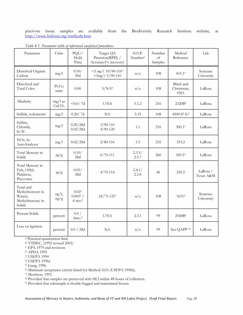
piscivore tissue samples are available from the Biodiversity Research Institute website, at http://www.briloon.org/methods.htm. Table 4.1. Parameter table of referenced analytical procedures.
Parameter
Units
PQLa/ Hold Time
Target QA
Precision(RPD) / Accuracy(% recovery)
S.O.P.
Numberb
Number
of Samples
Method
Reference
Lab
Dissolved Organic Carbon
mg/l
0.10/ 30d
<5 mg/l 10/90-1107
>5mg/l 5/90-110
n/a
108
415.11
Syracuse
University Dissolved and Total Color
Pt-Co units
0.00
5/NA8
n/a
108
Black and Christman,
1963.
LaRosa
Alkalinity
mg/l as CaCO3
<0.0/ 7d
1/NA
5.1.2
216
2320B2
LaRosa
Sulfide, iodometric
mg/l
0.20/ 7d
NA
5.15
108
4500-S2-E2
LaRosa
Sulfate, Chloride, by IC
mg/l
0.20/28d 0.02/28d
3/90-110 4/90-120
1.1
216
300.11
LaRosa
NOx, by AutoAnalyzer
mg/l
0.02/28d
2/80-116
1.5
216
353.2
LaRosa
Total Mercury in Solids
ug/g
0.10/ 28d
6/70-111
2.3.5/ 2.5.7
260
245.53
LaRosa
Total Mercury in Fish, Offal, Plankton, Piscovires
ug/g
0.05/ 28d
4/70-114
2.4.1/ 2.5.8
46
245.5
LaRosa /
Texas A&M
Total and Methylmercury in Waters, Methylmercury in Solids
ng/l, ng/g
0.025
0.0055 /6 mo.8
24/75-1257
n/a
108
16314
Syracuse
University
Percent Solids
percent
0.0 / 6mo.9
1/NA
2.3.1
99
2540B2
LaRosa
Loss on Ignition
percent
0.0 / 28d
NA
n/a
99
See QAPP 10
LaRosa
a) Practical quantitation limit b) VTDEC, (1992 revised 2001)1) EPA 1979 and revisions
2) APHA 1995 3) USEPA 1994 4) USEPA 1996a 5) Liang, 1996. 6) Minimum acceptance criteria listed for Method 1631 (USEPA 1996b). 7) Morrison, 1991. 8) Provided that samples are preserved with HCl within 48 hours of collection. 9) Provided that subsample is double bagged and maintained frozen.
Assessment of Mercury in Waters, Sediments, and Biota of VT and NH Lakes Project. Draft Final Report. Page 24
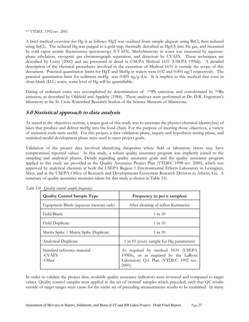
10) VTDEC 1992 rev. 2001 A brief method overview for Hg is as follows. HgT was oxidized from sample aliquots using BrCl, then reduced using SnCl2. The reduced Hg was purged to a gold trap, thermally desorbed as Hg(O) into He gas, and measured by cold vapor atomic fluorescence spectroscopy (CVAFS). Methylmercury in water was measured by aqueous-phase ethylation, cryogenic gas chromatograph separation, and detection by CVAFS. These techniques are described by Lorey (2002) and are presented in detail in USEPA Method 1631 (USEPA 1996b). A detailed description of the chemical procedures involved in the execution of Method 1631 is outside the scope of this document. Practical quantitation limits for HgT and MeHg in waters were 0.02 and 0.005 ng/l respectively. The practical quantitation limit for sediment meHg was 0.005 ng/g d.w. It is implicit in this method that even in clean blank (D.I.) water, some level of Hg will be quantifiable. Dating of sediment cores was accomplished by determination of 210Pb emission, and corroborated by 226Ra emission, as described by Oldfield and Appleby (1984). These analyses were performed at Dr. D.R. Engstrom’s laboratory at the St. Croix Watershed Research Station of the Science Museum of Minnesota. 5.0 Statistical approach to data analysis As stated in the objectives section, a major goal of this study was to ascertain the physico-chemical identity(ies) of lakes that produce and deliver meHg into the food chain. For the purpose of meeting those objectives, a variety of statistical tools were useful. For this project, a data validation phase, inquiry and hypothesis testing phase, and statistical model development phase were used to meet project goals. Validation of the project data involved identifying datapoints where field or laboratory errors may have compromised reported values. In this study, a robust quality assurance program was implicitly joined to the sampling and analytical phases. Details regarding quality assurance goals and the quality assurance program applied to this study are provided in the Quality Assurance Project Plan (VTDEC 1998 rev. 2000), which was approved by analytical chemists at both the USEPA Region 1 Environmental Effects Laboratory in Lexington, Mass, and at the USEPA Office of Research and Developments Ecosystem Research Division in Athens, Ga. A summary of quality assurance measures taken for this study is shown in Table 5.0. Table 5.0. Quality control sample frequency.
Quality Control Sample Type
Frequency (n per n samples)
Equipment Blank (aqueous mercury only)
After cleaning of teflon Kemmerer
Field Blank
1 in 10
Field Duplicate
1 in 10
Matrix Spike / Matrix Spike Duplicate
1 in 10
Analytical Duplicate
1 in 10 (every sample for Hg parameters)
Standard reference material -CVAFS -Other
As required by method 1631 (USEPA 1996b), or as required by the LaRosa Laboratory QA Plan (VTDEC 1992 rev. 2001)
In order to validate the project data, available quality assurance indicators were reviewed and compared to target values. Quality control samples were applied to the set of ‘normal’ samples which preceded, such that QC results outside of target ranges were cause for the entire set of preceding measurements results to be examined. In many
Assessment of Mercury in Waters, Sediments, and Biota of VT and NH Lakes Project. Draft Final Report. Page 25

cases, the cause of a poor QC sample result was traced to sampling or measurement error, and resulted in re-sampling or reanalysis. In this study, a common identified cause for poor duplicate results has been the sampling of hypolimnetic waters overly close to the microzone, where aqueous Hg results can be compromised by minute quantities of resuspended sediment in the sample. Results of the quality control and assurance program are reported in Section 7.0.
Assessment of Mercury in Waters, Sediments, and Biota of VT and NH Lakes Project. Draft Final Report. Page 26

6.0 Lakes sampled and data results 6.1 Study lakes Lakes sampled and data results are summarized in a series of tables within Section 6. Sampling for this project took place between June, 1998 and August, 2000. Project lakes were selected for initial sampling in either 1998 or 1999. In total, 93 lakes were sampled between 1998 and 1999, evenly split between years. A subset of 1998 lakes was resampled during 1999 and/or 2000 to verify out-of-control results, and to assess interannual variability. In addition, 13 lakes were sampled under the paleolimnology project, and 10 of these lakes were outside of the spatially randomized lake set. Table 6.1 provides a roster of the 103 unique study lakes, their geographic locations, initial sampling years, design blocks and weights, and matrices measured. The locations of these lakes are shown in Figure 6.1.
% %
$%
$%$ $ %% % %$%$ $$
% $$$ %
$$ %%
%%
$%
% $
% $ % % $% % $ %
% %
$$ % $
$ %
$
$%$
$ $
%$ %
$
$$%%%
%%$ $ %
$
%% $$
$
% $$ %%
$% %$%%
N
Figure 6.1. Geographic location of lakes sampled in conjunction with the Assessment of Hg in Sediment, Water, and Biota of VT and NH Lakes Project. Initial sampling year also shown ( ▲- 1998; ■- 1999).
Assessment of Mercury in Waters, Sediments, and Biota of VT and NH Lakes Project. Draft Final Report. Page 27
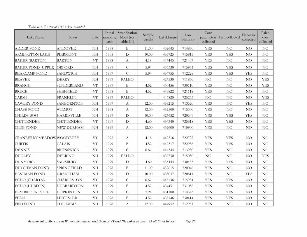
Table 6.1. Roster of 103 lakes sampled.
Lake Name Town State Initial
sampling year
Stratification block (see table 2.1)
Sample weight Lat ddmmss Lon
ddmmss
Core parameters collected
Fish collected Piscovire collected
Paleo core
collected
ADDER POND ANDOVER NH 1998 B 11.00 432645 714830 YES NO NO NOARMINGTON LAKE PIERMONT NH 1998 D 10.00 435725 715815 YES YES NO NO BAKER (BARTON) BARTON VT 1998 A 4.18 444445 721407 YES NO NO NO
BAKER POND- UPPER ORFORD NH 1999 C 5.94 435330 715934 YES YES NO NO BEARCAMP POND SANDWICH NH 1999 C 5.94 434755 712228 YES YES YES NO BEAVER DERRY NH 1999 PALEO 424530 711830 NO NO NO YES BRANCH SUNDERLAND VT 1999 B 4.52 430456 730110 YES NO NO YESBRUCE SHEFFIELD VT 1998 B 4.52 443822 721118 YES NO NO NOCARMI FRANKLIN VT 1999 PALEO 445820 725235 NO NO NO YESCAWLEY POND SANBORNTON NH 1999 A 12.00 433215 713620 YES NO YES NO CHASE POND WILMOT NH 1998 A 12.00 432500 715500 YES NO NO NOCHILDS BOG HARRISVILLE NH 1999 D 10.00 425652 720649 YES YES YES NO CHITTENDEN CHITTENDEN VT 1999 D 4.60 434340 725318 YES YES NO NOCLUB POND NEW DURHAM NH 1999 A 12.00 432600 710900 YES NO NO NO
CRANBERRY MEADOW WOODBURY VT 1998 A 4.18 442516 722727 YES YES NO NOCURTIS CALAIS VT 1999 B 4.52 442317 722938 YES YES NO NODENNIS BRUNSWICK VT 1999 C 6.67 444344 713930 YES NO NO NODUDLEY DEERING NH 1999 PALEO 430730 715030 NO NO NO YESDUNMORE SALISBURY VT 1999 D 4.60 435444 730435 YES YES NO NODUTCHMAN POND SPRINGFIELD NH 1998 B 11.00 432615 720046 YES NO NO NO EASTMAN POND GRANTHAM NH 1999 D 10.00 433037 720611 YES NO YES NO ECHO (CHARTN) CHARLESTON VT 1998 C 6.67 445136 715934 YES YES NO NOECHO (HUBDTN) HUBBARDTON VT 1999 B 4.52 434451 731058 YES YES NO NO ELM BROOK POOL HOPKINTON NH 1999 C 5.94 431100 714345 YES YES NO NOFERN LEICESTER VT 1998 B 4.52 435146 730414 YES YES NO NOFISH POND COLUMBIA NH 1998 A 12.00 444952 712931 YES NO NO NO
Assessment of Mercury in Waters, Sediments, and Biota of VT and NH Lakes Project. Draft Final Report. Page 28

Lake Name Town State Initial
sampling year
Stratification block (see table 2.1)
Sample weight Lat ddmmss Lon
ddmmss
Core parameters collected
Fish collected Piscovire collected
Paleo core
collected
FREESES POND- UPPER DEERFIELD NH 1998 A 12.00 430930 711400 YES NO NO NOGILES POND SANBORNTON NH 1999 A 12.00 432846 713851 YES YES NO NO GILMAN ALTON NH 1999 PALEO 433030 711200 NO NO NO YESGREAT HOSMER CRAFTSBURY VT 1999 D 4.60 444109 722152 YES YES NO NO
GREENWOOD POND KINGSTON NH 1999 B 11.00 425612 710343 YES YES YES NO
HALL POND- UPPER SANDWICH NH 1998 B 11.00 435054 713303 YES NO NO NO HARDWICK HARDWICK VT 1998 C 6.67 443118 722228 YES NO YES NOHARDWOOD ELMORE VT 1999 B 4.52 442804 723002 YES YES YES NOHIGH (SUDBRY) SUDBURY VT 1998 B 4.52 434510 730914 YES NO NO YES HILDRETH DAM POND WARREN NH 1998 A 12.00 435630 715325 YES NO NO NOHORN POND WAKEFIELD NH 1998 C 5.94 433342 705731 YES YES YES NOHORTONIA HUBBARDTON VT 1999 D 4.60 434519 731208 YES YES YES NOHOWE RESERVOIR DUBLIN NH 1999 C 5.94 425410 720634 YES YES NO NOINTERVALE SANDWICH NH 1999 PALEO 434730 713130 NO NO NO YESISLAND POND STODDARD NH 1998 C 5.94 430400 720456 YES YES NO NOIVANHOE- LAKE WAKEFIELD NH 1998 D 10.00 433605 705925 YES NO YES NOJACKSONVILLE WHITINGHAM VT 1998 A 4.18 424803 724900 YES YES YES NOJENNESS POND NORTHWOOD NH 1998 D 10.00 431525 711500 YES YES YES NO KENT SHERBURNE VT 1998 A 4.18 434032 724609 YES NO NO NOLARY POND CANAAN NH 1998 A 12.00 434230 720010 YES NO NO NO LEFFERTS CHITTENDEN VT 1999 A 4.18 434255 725411 YES YES NO NOLEVI GROTON VT 1999 B 4.52 441558 721341 YES NO NO NOLILY POND SOMERSWORTH NH 1998 B 11.00 431518 705460 YES NO NO NO LITTLE AVERILL AVERILL VT 1999 D 4.60 445702 714256 YES NO YES NOLONG (WESTMR) WESTMORE VT 1999 B 4.52 444506 720103 YES NO YES NOLOON LAKE PLYMOUTH NH 1999 C 5.94 434637 714509 YES YES NO NOLOVELL LAKE- STN 1 WAKEFIELD NH 1999 D 10.00 433144 710118 YES YES YES NO
Assessment of Mercury in Waters, Sediments, and Biota of VT and NH Lakes Project. Draft Final Report. Page 29
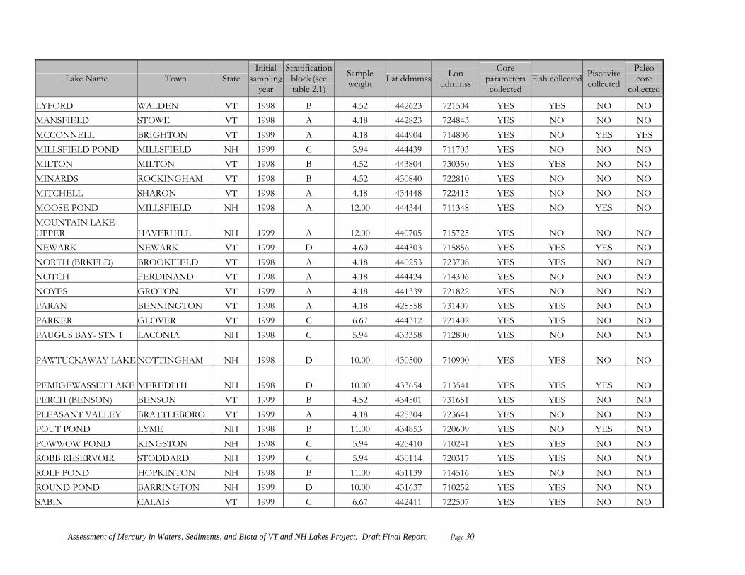
Lake Name Town State Initial
sampling year
Stratification block (see table 2.1)
Sample weight Lat ddmmss Lon
ddmmss
Core parameters collected
Fish collected Piscovire collected
Paleo core
collected
LYFORD WALDEN VT 1998 B 4.52 442623 721504 YES YES NO NOMANSFIELD STOWE VT 1998 A 4.18 442823 724843 YES NO NO NOMCCONNELL BRIGHTON VT 1999 A 4.18 444904 714806 YES NO YES YESMILLSFIELD POND MILLSFIELD NH 1999 C 5.94 444439 711703 YES NO NO NO MILTON MILTON VT 1998 B 4.52 443804 730350 YES YES NO NOMINARDS ROCKINGHAM VT 1998 B 4.52 430840 722810 YES NO NO NOMITCHELL SHARON VT 1998 A 4.18 434448 722415 YES NO NO NOMOOSE POND MILLSFIELD NH 1998 A 12.00 444344 711348 YES NO YES NO MOUNTAIN LAKE- UPPER HAVERHILL NH 1999 A 12.00 440705 715725 YES NO NO NO NEWARK NEWARK VT 1999 D 4.60 444303 715856 YES YES YES NONORTH (BRKFLD) BROOKFIELD VT 1998 A 4.18 440253 723708 YES YES NO NONOTCH FERDINAND VT 1998 A 4.18 444424 714306 YES NO NO NONOYES GROTON VT 1999 A 4.18 441339 721822 YES NO NO NOPARAN BENNINGTON VT 1998 A 4.18 425558 731407 YES YES NO NOPARKER GLOVER VT 1999 C 6.67 444312 721402 YES YES NO NOPAUGUS BAY- STN 1 LACONIA NH 1998 C 5.94 433358 712800 YES NO NO NO
PAWTUCKAWAY LAKE NOTTINGHAM NH 1998 D 10.00 430500 710900 YES YES NO NO
PEMIGEWASSET LAKE MEREDITH NH 1998 D 10.00 433654 713541 YES YES YES NO PERCH (BENSON) BENSON VT 1999 B 4.52 434501 731651 YES YES NO NO PLEASANT VALLEY BRATTLEBORO VT 1999 A 4.18 425304 723641 YES NO NO NO POUT POND LYME NH 1998 B 11.00 434853 720609 YES NO YES NOPOWWOW POND KINGSTON NH 1998 C 5.94 425410 710241 YES YES NO NOROBB RESERVOIR STODDARD NH 1999 C 5.94 430114 720317 YES YES NO NOROLF POND HOPKINTON NH 1998 B 11.00 431139 714516 YES NO NO NO ROUND POND BARRINGTON NH 1999 D 10.00 431637 710252 YES YES NO NO SABIN CALAIS VT 1999 C 6.67 442411 722507 YES YES NO NO
Assessment of Mercury in Waters, Sediments, and Biota of VT and NH Lakes Project. Draft Final Report. Page 30

Lake Name Town State Initial
sampling year
Stratification block (see table 2.1)
Sample weight Lat ddmmss Lon
ddmmss
Core parameters collected
Fish collected Piscovire collected
Paleo core
collected
SESSIONS DUMMER NH 1999 PALEO 444220 711150 NO NO NO YES SHAWS POND NEW DURHAM NH 1999 A 12.00 433060 710906 YES NO NO NO SILVER LAKE HARRISVILLE NH 1998 D 10.00 425730 720825 YES YES NO NO SOMERSET SOMERSET VT 1998 D 4.60 425832 725652 YES YES YES NOSOUTH AMERICA FERDINAND VT 1998 A 4.18 444218 714442 YES NO NO NOSPRING (SHRWBY) SHREWSBURY VT 1999 PALEO 432942 725512 NO NO NO YES SPRUCE POND DEERFIELD NH 1999 B 11.00 430609 712047 YES NO NO NO STRATTON STRATTON VT 1998 B 4.52 430617 725810 YES NO NO NOSUNCOOK POND- UPPER BARNSTEAD NH 1998 C 5.94 432319 711710 YES YES YES NOSUNRISE LAKE MIDDLETON NH 1999 D 10.00 432715 710430 YES YES YES NO SUNSET (BRKFLD) BROOKFIELD VT 1999 A 4.18 440237 723614 YES YES NO NOTRIO PONDS- ONE AND TWO ODELL NH 1998 B 11.00 444240 712200 YES NO NO NOTUTTLE (HARDWK) HARDWICK VT 1998 B 4.52 443330 721836 YES NO NO NOUNNAMED POND DEERING NH 1999 B 11.00 430320 715220 YES NO NO NO WALKER POND BOSCAWEN NH 1999 C 5.94 431804 714059 YES YES YES NO WALLINGFORD WALLINGFORD VT 1999 PALEO 432341 725432 NO NO NO YES
WHEELER (BRUNWK) BRUNSWICK VT 1999 PALEO 444230 713829 NO NO NO YESWILLARD ANTRIM NH 1999 PALEO 430130 720130 NO NO NO YESWILLEY POND- BIG STRAFFORD NH 1999 A 12.00 431646 711107 YES NO NO NOWILLEY POND- LITTLE STRAFFORD NH 1999 B 11.00 431735 711040 YES NO NO NOWILLOUGHBY WESTMORE VT 1998 D 4.60 444506 720344 YES YES YES NOWILSON POND SWANZEY NH 1999 B 11.00 425402 721544 YES YES NO NO WOLCOTT WOLCOTT VT 1999 B 4.52 443355 722516 YES YES YES NO
ZEPHYR LAKE GREENFIELD NH 1998 B 11.00 425603 715123 YES YES YES NO
Assessment of Mercury in Waters, Sediments, and Biota of VT and NH Lakes Project. Draft Final Report. Page 31

6.2 Water chemistry for core sampling lakes Water chemistry results are summarized by lake zone (epilimnion and hypolimnion), and are calculated from both raw and geographically weighted data. Incorporation of geographic sample weights (Table 6.1) accounts for the density of lakes in geographic proximity to the target sampling lake. Thus, statistics based on raw data summarize only the current dataset, while statistics based on weighted datapoints provide geographically unbiased estimates for all lakes in Vermont and New Hampshire. Water chemistry results for aqueous parameters are presented in Table 6.2. Table 6.2. Summary of water chemistry data.
Summary statistics based on raw data
Parameter Strata Count Min. Mean Median Max. Range St. error 95% lower C.L.
95% upper C. L.
Acid Neut. Capacity EPI 127 -1.10 26.03 8.10 198.00 199.10 3.28 19.54 32.52 Acid Neut. Capacity HYP 75 0.23 30.62 11.60 151.00 150.77 4.21 22.23 39.00 CL-_mg/l EPI 129 0.10 7.44 3.28 45.70 45.60 0.84 5.77 9.11 CL-_mg/l HYP 80 0.21 7.54 2.57 52.20 51.99 1.24 5.06 10.01 Diss. Color PtCo units EPI 90 0.20 29.61 17.45 216.00 215.80 3.68 22.29 36.93 Diss. Color PtCo units HYP 55 3.90 45.00 24.00 210.00 206.10 6.64 31.68 58.32 DOC mg/l EPI 130 0.35 4.26 3.59 13.30 12.95 0.18 3.90 4.62 DOC mg/l HYP 80 1.29 3.83 3.19 11.30 10.01 0.22 3.39 4.27 HgT_ng/l EPI 129 0.22 1.74 1.23 9.66 9.44 0.13 1.47 2.00 HgT_ng/l HYP 68 1.13 10.40 7.07 34.54 33.41 1.12 8.17 12.62 MeHg_ng/l EPI 129 0.038 0.291 0.239 3.120 3.082 0.027 0.238 0.345 MeHg_ng/l HYP 68 0.051 0.814 0.409 4.454 4.403 0.121 0.573 1.054 NOx_mg/l EPI 128 0.02 0.03 0.02 0.33 0.31 0.00 0.03 0.04 NOx_mg/l HYP 80 0.02 0.04 0.02 0.24 0.22 0.00 0.03 0.05 SO4_mg/l EPI 129 1.95 4.20 3.92 10.00 8.05 0.13 3.94 4.45 SO4_mg/l HYP 80 0.90 4.09 3.68 12.80 11.90 0.21 3.67 4.51 Sulfide_mg/l EPI 44 0.02 0.10 0.02 1.40 1.38 0.03 0.04 0.17 Sulfide_mg/l HYP 72 0.02 0.14 0.03 1.30 1.28 0.03 0.08 0.19 Total Color PtCo units EPI 127 5.00 43.46 32.70 227.00 222.00 3.36 36.81 50.11 Total Color PtCo units HYP 78 4.70 72.37 52.00 272.00 267.30 6.74 58.96 85.79
Summary statistics based on individual lake weights
Acid Neut. Capacity EPI 127 -1.1 19.1 6.4 198.0 199.1 1.0 17.1 21.1 Acid Neut. Capacity HYP 75 0.2 24.1 10.3 151.0 150.8 1.5 21.2 27.0 CL-_mg/l EPI 129 0.10 8.09 4.18 45.70 45.60 0.32 7.46 8.72 CL-_mg/l HYP 80 0.21 7.84 3.02 52.20 51.99 0.47 6.93 8.76 Diss. Color PtCo units EPI 90 0.20 27.10 17.00 216.00 215.80 1.35 24.46 29.74 Diss. Color PtCo units HYP 55 3.90 41.24 22.40 210.00 206.10 2.61 36.11 46.38 DOC mg/l EPI 130 0.35 4.31 3.70 13.30 12.95 0.07 4.18 4.44 DOC mg/l HYP 80 1.29 3.91 3.60 11.30 10.01 0.08 3.75 4.07 HgT_ng/l EPI 129 0.22 1.78 1.31 9.66 9.44 0.05 1.68 1.88 HgT_ng/l HYP 68 1.13 11.52 7.70 34.54 33.41 0.46 10.62 12.41 MeHg_ng/l EPI 129 0.038 0.299 0.259 3.120 3.082 0.009 0.281 0.318 MeHg_ng/l HYP 68 0.051 0.829 0.402 4.454 4.403 0.047 0.738 0.921 NOX_mg/l EPI 128 0.02 0.03 0.02 0.33 0.31 0.00 0.03 0.04
Assessment of Mercury in Waters, Sediments, and Biota of VT and NH Lakes Project. Draft Final Report. Page 32
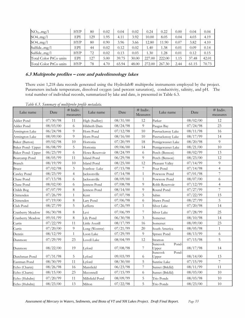
NOX_mg/l HYP 80 0.02 0.04 0.02 0.24 0.22 0.00 0.04 0.04 SO4_mg/l EPI 129 1.95 4.11 3.92 10.00 8.05 0.04 4.03 4.19 SO4_mg/l HYP 80 0.90 3.96 3.66 12.80 11.90 0.07 3.82 4.10 Sulfide_mg/l EPI 44 0.02 0.12 0.02 1.40 1.38 0.01 0.09 0.14 Sulfide_mg/l HYP 72 0.02 0.13 0.03 1.30 1.28 0.01 0.12 0.15 Total Color PtCo units EPI 127 5.00 39.75 30.00 227.00 222.00 1.15 37.48 42.01 Total Color PtCo units HYP 78 4.70 65.94 48.00 272.00 267.30 2.44 61.15 70.73
6.3 Multiprobe profiles – core and paleolimnology lakes There exist 1,218 data records generated using the Hydrolab® multiprobe instruments employed by the project. Parameters include temperature, dissolved oxygen (and percent saturation), conductivity, salinity, and pH. The total number of individual records, summarized by lake and date, is presented in Table 6.3. Table 6.3. Summary of multiprobe profile metadata.
Lake name Date # Indiv. measures Lake name Date # Indiv.
Measures Lake name Date # Indiv. measures
Adder Pond 07/30/98 11 High (Sudbry) 08/31/00 12 Parker 08/02/00 12 Adder Pond 08/03/00 6 Hildreth Dam 08/24/98 9 Paugus Bay 07/24/98 23 Armington Lake 06/24/98 9 Horn Pond 07/12/98 10 Pawtuckaway Lake 08/11/98 16 Armington Lake 08/09/00 9 Horn Pond 08/16/00 10 Pawtuckaway Lake 08/17/99 14 Baker (Barton) 09/02/98 10 Hortonia 07/20/99 18 Pemigewasset Lake 08/20/98 9 Baker Pond- Upper 06/08/99 5 Hortonia 09/06/00 14 Pemigewasset Lake 08/21/00 10 Baker Pond- Upper 06/23/99 6 Howe Reservoir 08/24/99 6 Perch (Benson) 08/02/99 13 Bearcamp Pond 08/05/99 11 Island Pond 06/29/98 9 Perch (Benson) 08/23/00 12 Branch 08/19/99 10 Island Pond 08/25/00 12 Pleasant Valley 07/14/99 9 Bruce 07/02/98 3 Ivanhoe- Lake 07/15/98 7 Pout Pond 07/14/98 4 Cawley Pond 08/23/99 4 Jacksonville 07/14/98 1 Powwow Pond 07/01/98 7 Chase Pond 07/13/98 6 Jacksonville 08/09/00 1 Powwow Pond 08/07/00 6 Chase Pond 08/02/00 6 Jenness Pond 07/08/98 9 Robb Reservoir 07/12/99 4 Childs Bog 07/07/99 8 Jenness Pond 08/14/00 9 Round Pond 07/27/99 7 Chittenden 07/26/99 1 Kent 07/07/98 5 Sabin 07/22/99 15 Chittenden 07/19/00 8 Lary Pond 07/06/98 6 Shaws Pond 08/27/99 5 Club Pond 08/27/99 5 Lefferts 07/26/99 1 Silver Lake 07/20/98 14
Cranberry Meadow 06/30/98 8 Levi 07/06/99 7 Silver Lake 07/28/99 25 Cranberry Meadow 09/01/99 8 Lily Pond 06/30/98 3 Somerset 08/10/98 14 Curtis 07/22/99 11 Little Averill 08/17/99 16 Somerset 08/09/00 23 Curtis 07/20/00 9 Long (Westmr) 07/21/99 20 South America 08/05/98 1 Dennis 08/12/99 1 Loon Lake 07/29/99 9 Spruce Pond 08/13/99 6 Dunmore 07/29/99 23 Lovell Lake 08/04/99 12 Stratton 07/15/98 5
Dunmore 08/22/00 19 Lyford 07/08/98 7 Suncook Pond-Upper 08/17/98 14
Dutchman Pond 07/31/98 5 Lyford 09/03/99 6 Suncook Pond-Upper 08/14/00 13
Eastman Pond 08/30/99 11 Lyford 08/30/00 5 Sunrise Lake 07/15/99 7 Echo (Chartn) 08/26/98 16 Mansfield 06/23/98 7 Sunset (Brkfld) 08/11/99 11 Echo (Chartn) 08/15/00 23 Mcconnell 07/15/99 6 Sunset (Brkfld) 08/03/00 10 Echo (Hubdtn) 07/20/99 11 Millsfield Pond 08/09/99 5 Trio Ponds 08/03/98 10 Echo (Hubdtn) 08/23/00 13 Milton 07/22/98 5 Trio Ponds 08/23/00 10
Assessment of Mercury in Waters, Sediments, and Biota of VT and NH Lakes Project. Draft Final Report. Page 33

Lake name Date # Indiv. measures Lake name Date # Indiv.
Measures Lake name Date # Indiv. measures
Elm Brook Pool 08/19/99 6 Milton 08/24/00 4 Tuttle (Hardwk) 07/01/98 1 Fern 07/23/98 13 Minards 07/29/98 14 Unnamed Pond 07/14/99 3 Fern 07/29/99 13 Minards 09/01/00 15 Walker Pond 08/16/99 13 Fern 08/22/00 13 Mitchell 09/09/98 4 Willey Pond- Big 07/22/99 8 Fish Pond 08/04/98 5 Moose Pond 08/05/98 5 Willey Pond- Little 07/22/99 5 Freeses Pond-Upper 07/08/98 5 Mountain Lake 08/09/99 6 Willoughby 08/14/98 19
Giles Pond 08/23/99 6 Newark 07/21/99 9 Willoughby 08/08/00 32 Great Hosmer 07/27/99 13 North (Brkfld) 07/20/98 5 Wilson Pond 08/03/99 5 Great Hosmer 08/30/00 14 North (Brkfld) 08/03/00 4 Wolcott 08/24/99 7 Greenwood Pond 07/19/99 8 Notch 08/05/98 9 Wolcott 08/02/00 7 Hall Pond- Upper 08/19/98 14 Notch 08/16/00 8 Zephyr Lake 07/27/98 11 Hardwick 07/28/98 4 Noyes 07/07/99 3 Zephyr Lake 08/24/99 6 Hardwood 07/01/99 4 Paran 07/14/98 5 Hardwood 08/02/00 5 Paran 08/09/00 5 High (Sudbry) 07/30/98 17 Parker 07/27/99 13
6.4 Sediment chemistry – core lakes Sediment chemistry summary statistics were calculated from both raw and geographically weighted data, for percent solids and loss on ignition, HgT, meHg, and percent of total Hg as meHg. These statistics are presented in Table 6.4. Table 6.4. Summary of sediment chemistry data.
Summary statistics based on raw data
Parameter Count Min. Mean Median Max. Range St. error 95% lower C.L.
95% upper C. L.
Sediment HgT - ug/g 129 0.07 0.24 0.22 0.62 0.55 0.01 0.22 0.26 Sediment meHG - ug/g 78 0.0004 0.004 0.003 0.021 0.021 0.0001 0.004 0.005 Sediment meHG, % of HgT 78 0.240 1.842 1.462 7.840 7.600 0.156 1.530 2.154 Solid content % 129 1.56 8.01 6.50 43.90 42.34 0.48 7.07 8.95 Loss on ignition % 129 9.20 32.56 30.60 69.20 60.00 1.11 30.36 34.75
Summary statistics based on individual lake weights
Sediment HgT - ug/g 129 0.07 0.24 0.21 0.62 0.55 0.00 0.23 0.25 Sediment meHG - ug/g † 78 0.0004 0.004 0.003 0.021 0.021 0.0001 0.004 0.004 Sediment meHG, % of HgT † 78 0.240 1.713 1.430 7.840 7.600 0.054 1.607 1.818 Solid content % 129 1.56 8.35 7.00 43.90 42.34 0.19 7.97 8.72 Loss on ignition % 129 9.20 32.17 30.50 69.20 60.00 0.39 31.40 32.95
†) please refer to section 7.4 for a discussion regarding the quality of the sediment meHg data results.
Assessment of Mercury in Waters, Sediments, and Biota of VT and NH Lakes Project. Draft Final Report. Page 34
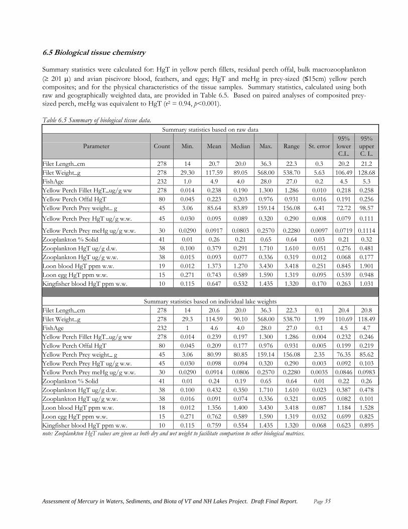
6.5 Biological tissue chemistry Summary statistics were calculated for: HgT in yellow perch fillets, residual perch offal, bulk macrozooplankton (≥ 201 µ) and avian piscivore blood, feathers, and eggs; HgT and meHg in prey-sized (≤15cm) yellow perch composites; and for the physical characteristics of the tissue samples. Summary statistics, calculated using both raw and geographically weighted data, are provided in Table 6.5. Based on paired analyses of composited prey-sized perch, meHg was equivalent to HgT (r2 = 0.94, p<0.001). Table 6.5 Summary of biological tissue data.
Summary statistics based on raw data
Parameter Count Min. Mean Median Max. Range St. error95% lower C.L.
95% upper C. L.
Filet Length_cm 278 14 20.7 20.0 36.3 22.3 0.3 20.2 21.2 Filet Weight_g 278 29.30 117.59 89.05 568.00 538.70 5.63 106.49 128.68FishAge 232 1.0 4.9 4.0 28.0 27.0 0.2 4.5 5.3 Yellow Perch Fillet HgT_ug/g ww 278 0.014 0.238 0.190 1.300 1.286 0.010 0.218 0.258 Yellow Perch Offal HgT 80 0.045 0.223 0.203 0.976 0.931 0.016 0.191 0.256 Yellow Perch Prey weight_ g 45 3.06 85.64 83.89 159.14 156.08 6.41 72.72 98.57 Yellow Perch Prey HgT ug/g w.w. 45 0.030 0.095 0.089 0.320 0.290 0.008 0.079 0.111
Yellow Perch Prey meHg ug/g w.w. 30 0.0290 0.0917 0.0803 0.2570 0.2280 0.0097 0.0719 0.1114Zooplankton % Solid 41 0.01 0.26 0.21 0.65 0.64 0.03 0.21 0.32 Zooplankton HgT ug/g d.w. 38 0.100 0.379 0.291 1.710 1.610 0.051 0.276 0.481 Zooplankton HgT ug/g w.w. 38 0.015 0.093 0.077 0.336 0.319 0.012 0.068 0.177 Loon blood HgT ppm w.w. 19 0.012 1.373 1.270 3.430 3.418 0.251 0.845 1.901 Loon egg HgT ppm w.w. 15 0.271 0.743 0.589 1.590 1.319 0.095 0.539 0.948 Kingfisher blood HgT ppm w.w. 10 0.115 0.647 0.532 1.435 1.320 0.170 0.263 1.031
Summary statistics based on individual lake weights
Filet Length_cm 278 14 20.6 20.0 36.3 22.3 0.1 20.4 20.8 Filet Weight_g 278 29.3 114.59 90.10 568.00 538.70 1.99 110.69 118.49FishAge 232 1 4.6 4.0 28.0 27.0 0.1 4.5 4.7 Yellow Perch Fillet HgT_ug/g ww 278 0.014 0.239 0.197 1.300 1.286 0.004 0.232 0.246 Yellow Perch Offal HgT 80 0.045 0.209 0.177 0.976 0.931 0.005 0.199 0.219 Yellow Perch Prey weight_ g 45 3.06 80.99 80.85 159.14 156.08 2.35 76.35 85.62 Yellow Perch Prey HgT ug/g w.w. 45 0.030 0.098 0.094 0.320 0.290 0.003 0.092 0.103 Yellow Perch Prey meHg ug/g w.w. 30 0.0290 0.0914 0.0806 0.2570 0.2280 0.0035 0.0846 0.0983Zooplankton % Solid 41 0.01 0.24 0.19 0.65 0.64 0.01 0.22 0.26 Zooplankton HgT ug/g d.w. 38 0.100 0.432 0.350 1.710 1.610 0.023 0.387 0.478 Zooplankton HgT ug/g w.w. 38 0.016 0.091 0.074 0.336 0.321 0.005 0.082 0.101 Loon blood HgT ppm w.w. 18 0.012 1.356 1.400 3.430 3.418 0.087 1.184 1.528 Loon egg HgT ppm w.w. 15 0.271 0.762 0.589 1.590 1.319 0.032 0.699 0.825 Kingfisher blood HgT ppm w.w. 10 0.115 0.759 0.554 1.435 1.320 0.068 0.623 0.895 note: Zooplankton HgT values are given as both dry and wet weight to facilitate comparison to other biological matrices.
Assessment of Mercury in Waters, Sediments, and Biota of VT and NH Lakes Project. Draft Final Report. Page 35

6.6. Risk characterizations to common loons Tissue samples acquired from common loons permit assessment of the overall risk to loons posed by Hg bioaccumulation. Risk characterizations were derived using either adult or juvenile blood, or abandoned eggs. The type of sample acquired was determined in the field based on availability and opportunity. Risk attributions followed the protocols of Evers et al. (2000). Based on these characterizations, samples collected from lakes in this study were evaluated by state, and in relation to loon tissues acquired from the Maine REMAP study lakes (MEDEP, 1995). Results are provided in Figure 6.6. Fifty percent of loons from Vermont study lakes, and 70% of loons from NH study lakes, have sufficient Hg in their tissues so as to pose a moderate or greater risk to the animals themselves. In Maine, that proportion is 78%. The total percentages of birds at high or extra high risk increases from 20% in VT to 27% in Maine. A geographic gradient is apparent in these data, with a clear increase from west to east. This is consistent with the findings of Evers et al. (1998).
50%
30%
22%
30%
47%
51%
10%
19%
20%
10%
4%
7%
0% 10% 20% 30% 40% 50% 60% 70% 80% 90% 100%
ME-REMAP (n=82)
NH-REMAP (n=57)
VT-REMAP (n=20)
Low risk Moderate risk High Risk Extra high risk
Figure 6.6. Mercury risk to breeding Common Loons (Gavia immer), based on adult and juvenile blood and egg Hglevels.
Evers (e.g., 2003 in prep.) further indicates that these risk proportions are sufficient so as to threaten entire loon populations. The present hypothesis regarding population-level impacts on loons is that chronic Hg exposure impacts to loons is reducing the ability of loon pair to successfully produce chicks, owing to impacts to individual birds within the parent pair (Evers, pers. comm.). Individual-level impacts include reduced ability to acquire food for chicks, and reduced ability to defend nesting territories from predators and other loons. However, in the field, observations regarding loon nesting habits from citizen monitoring groups continue to show increases in overall numbers of nesting loon pair. While these two phenomena seem at odds, they are in fact consistent, when the effect of the male loon “buffer population” is accounted for. The “buffer population” is that group of male birds (typically juvenile or subadult, lone birds) that is available to fill in for a nesting male bird, if that bird is unable to successfully defend its territory, or is lost due to disease or other factors. It is the decline in the “buffer population” that is cause for concern. Declines in actual nesting loon pair and reared chicks is expected to accompany further reductions in the buffer population.
Assessment of Mercury in Waters, Sediments, and Biota of VT and NH Lakes Project. Draft Final Report. Page 36
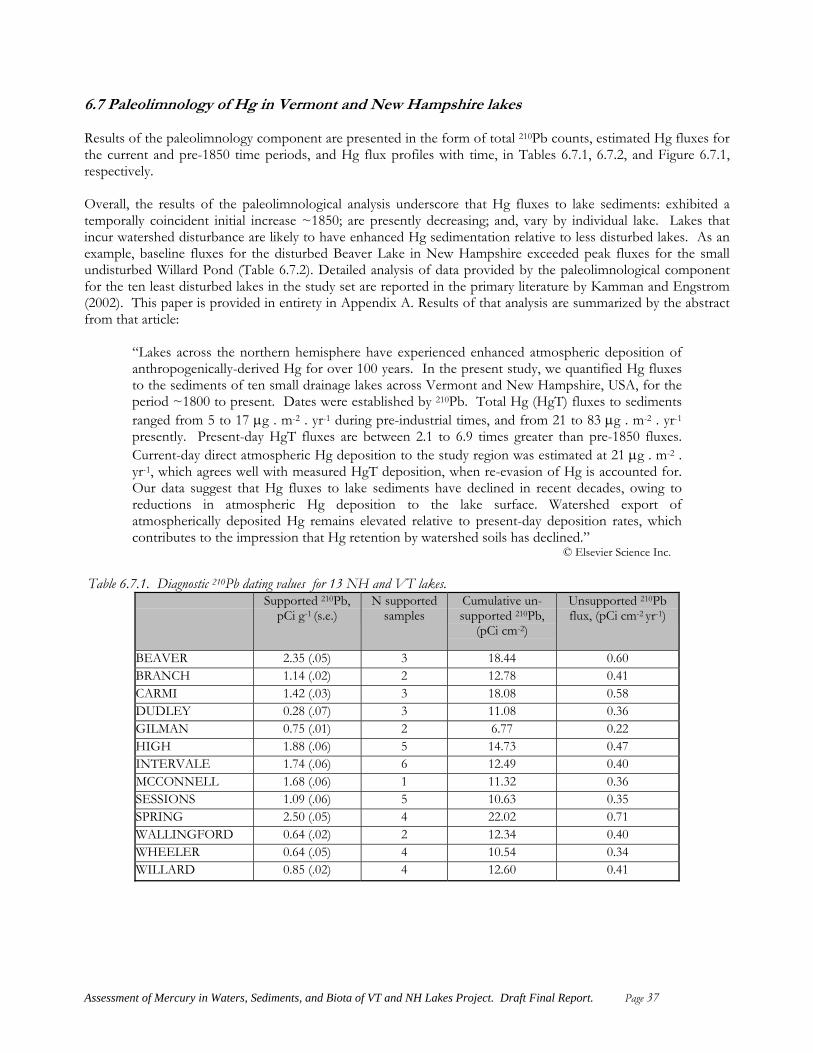
6.7 Paleolimnology of Hg in Vermont and New Hampshire lakes Results of the paleolimnology component are presented in the form of total 210Pb counts, estimated Hg fluxes for the current and pre-1850 time periods, and Hg flux profiles with time, in Tables 6.7.1, 6.7.2, and Figure 6.7.1, respectively. Overall, the results of the paleolimnological analysis underscore that Hg fluxes to lake sediments: exhibited a temporally coincident initial increase ~1850; are presently decreasing; and, vary by individual lake. Lakes that incur watershed disturbance are likely to have enhanced Hg sedimentation relative to less disturbed lakes. As an example, baseline fluxes for the disturbed Beaver Lake in New Hampshire exceeded peak fluxes for the small undisturbed Willard Pond (Table 6.7.2). Detailed analysis of data provided by the paleolimnological component for the ten least disturbed lakes in the study set are reported in the primary literature by Kamman and Engstrom (2002). This paper is provided in entirety in Appendix A. Results of that analysis are summarized by the abstract from that article:
“Lakes across the northern hemisphere have experienced enhanced atmospheric deposition of anthropogenically-derived Hg for over 100 years. In the present study, we quantified Hg fluxes to the sediments of ten small drainage lakes across Vermont and New Hampshire, USA, for the period ~1800 to present. Dates were established by 210Pb. Total Hg (HgT) fluxes to sediments ranged from 5 to 17 µg . m-2 . yr-1 during pre-industrial times, and from 21 to 83 µg . m-2 . yr-1 presently. Present-day HgT fluxes are between 2.1 to 6.9 times greater than pre-1850 fluxes. Current-day direct atmospheric Hg deposition to the study region was estimated at 21 µg . m-2 . yr-1, which agrees well with measured HgT deposition, when re-evasion of Hg is accounted for. Our data suggest that Hg fluxes to lake sediments have declined in recent decades, owing to reductions in atmospheric Hg deposition to the lake surface. Watershed export of atmospherically deposited Hg remains elevated relative to present-day deposition rates, which contributes to the impression that Hg retention by watershed soils has declined.” © Elsevier Science Inc.
Table 6.7.1. Diagnostic 210Pb dating values for 13 NH and VT lakes.
Supported 210Pb, pCi g-1 (s.e.)
N supported samples
Cumulative un-supported 210Pb,
(pCi cm-2)
Unsupported 210Pb flux, (pCi cm-2 yr-1)
BEAVER 2.35 (.05) 3 18.44 0.60 BRANCH 1.14 (.02) 2 12.78 0.41 CARMI 1.42 (.03) 3 18.08 0.58 DUDLEY 0.28 (.07) 3 11.08 0.36 GILMAN 0.75 (.01) 2 6.77 0.22 HIGH 1.88 (.06) 5 14.73 0.47 INTERVALE 1.74 (.06) 6 12.49 0.40 MCCONNELL 1.68 (.06) 1 11.32 0.36 SESSIONS 1.09 (.06) 5 10.63 0.35 SPRING 2.50 (.05) 4 22.02 0.71 WALLINGFORD 0.64 (.02) 2 12.34 0.40 WHEELER 0.64 (.05) 4 10.54 0.34 WILLARD 0.85 (.02) 4 12.60 0.41
Assessment of Mercury in Waters, Sediments, and Biota of VT and NH Lakes Project. Draft Final Report. Page 37
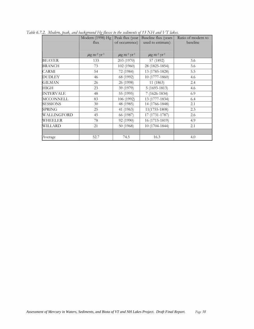
Table 6.7.2. Modern, peak, and background Hg fluxes to the sediments of 13 NH and VT lakes. Modern (1998) Hg
flux Peak flux (year of occurrence)
Baseline flux (years used to estimate)
µg m-2 yr-1 µg m-2 yr-1 µg m-2 yr-1
Ratio of modern to baseline
BEAVER 133 203 (1970) 57 (1892) 3.6 BRANCH 73 102 (1960) 28 (1825-1854) 3.6 CARMI 54 72 (1984) 13 (1785-1828) 5.5 DUDLEY 46 68 (1992) 10 (1777-1860) 4.6 GILMAN 26 26 (1998) 11 (1863) 2.4 HIGH 23 39 (1979) 5 (1693-1813) 4.6 INTERVALE 48 55 (1995) 7 (1626-1834) 6.9 MCCONNELL 83 106 (1992) 13 (1777-1834) 6.4 SESSIONS 30 48 (1985) 14 (1766-1848) 2.1 SPRING 25 41 (1963) 11(1755-1808) 2.3 WALLINGFORD 45 66 (1987) 17 (1731-1787) 2.6 WHEELER 78 92 (1990) 16 (1715-1819) 4.9 WILLARD 21 50 (1968) 10 (1704-1844) 2.1 Average 52.7 74.5 16.3 4.0
Assessment of Mercury in Waters, Sediments, and Biota of VT and NH Lakes Project. Draft Final Report. Page 38

Spring Lake
210 P
b D
ate
1800
1850
1900
1950
2000Lake Carmi High Pond Branch Pond Willard Pond
Sessions Pond
210 P
b D
ate
1800
1850
1900
1950
2000 Wallingford Pond Gilman Pond Intervale Pond McConnell Pond
Beaver Lake
0 50 100 150 200
210 P
b D
ate
1800
1850
1900
1950
2000Wheeler Pond
Hg Flux (ug . m-2 . yr-1)
0 50 100 150
210 P
b D
ate
1800
1850
1900
1950
2000Dudley Pond
0 50 100 150
Figure 6.7. 210Pb-inferred Hg fluxes to the sediments of 13 VT and NH lakes. X-axis scaling for Wheeler and Dudley Ponds applies to all unlabelled axes.
Assessment of Mercury in Waters, Sediments, and Biota of VT and NH Lakes Project. Draft Final Report. Page 39
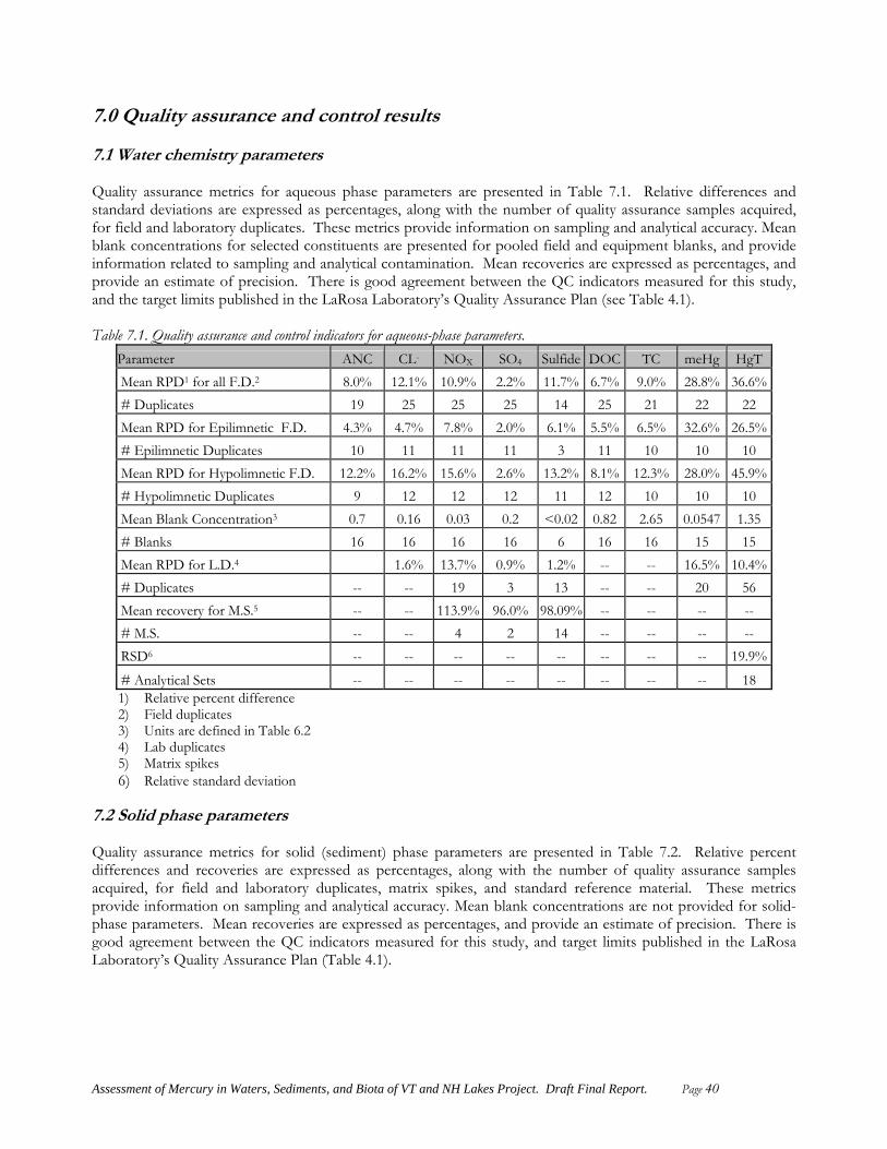
7.0 Quality assurance and control resul s t 7.1 Water chemistry parameters Quality assurance metrics for aqueous phase parameters are presented in Table 7.1. Relative differences and standard deviations are expressed as percentages, along with the number of quality assurance samples acquired, for field and laboratory duplicates. These metrics provide information on sampling and analytical accuracy. Mean blank concentrations for selected constituents are presented for pooled field and equipment blanks, and provide information related to sampling and analytical contamination. Mean recoveries are expressed as percentages, and provide an estimate of precision. There is good agreement between the QC indicators measured for this study, and the target limits published in the LaRosa Laboratory’s Quality Assurance Plan (see Table 4.1). Table 7.1. Quality assurance and control indicators for aqueous-phase parameters.
Parameter ANC CL- NOX SO4 Sulfide DOC TC meHg HgT Mean RPD1 for all F.D.2 8.0% 12.1% 10.9% 2.2% 11.7% 6.7% 9.0% 28.8% 36.6% # Duplicates 19 25 25 25 14 25 21 22 22 Mean RPD for Epilimnetic F.D. 4.3% 4.7% 7.8% 2.0% 6.1% 5.5% 6.5% 32.6% 26.5% # Epilimnetic Duplicates 10 11 11 11 3 11 10 10 10 Mean RPD for Hypolimnetic F.D. 12.2% 16.2% 15.6% 2.6% 13.2% 8.1% 12.3% 28.0% 45.9% # Hypolimnetic Duplicates 9 12 12 12 11 12 10 10 10 Mean Blank Concentration3 0.7 0.16 0.03 0.2 <0.02 0.82 2.65 0.0547 1.35 # Blanks 16 16 16 16 6 16 16 15 15 Mean RPD for L.D.4 1.6% 13.7% 0.9% 1.2% -- -- 16.5% 10.4% # Duplicates -- -- 19 3 13 -- -- 20 56 Mean recovery for M.S.5 -- -- 113.9% 96.0% 98.09% -- -- -- -- # M.S. -- -- 4 2 14 -- -- -- -- RSD6 -- -- -- -- -- -- -- -- 19.9%
# Analytical Sets -- -- -- -- -- -- -- -- 18 1) Relative percent difference 2) Field duplicates 3) Units are defined in Table 6.2 4) Lab duplicates 5) Matrix spikes 6) Relative standard deviation
7.2 Solid phase parameters Quality assurance metrics for solid (sediment) phase parameters are presented in Table 7.2. Relative percent differences and recoveries are expressed as percentages, along with the number of quality assurance samples acquired, for field and laboratory duplicates, matrix spikes, and standard reference material. These metrics provide information on sampling and analytical accuracy. Mean blank concentrations are not provided for solid-phase parameters. Mean recoveries are expressed as percentages, and provide an estimate of precision. There is good agreement between the QC indicators measured for this study, and target limits published in the LaRosa Laboratory’s Quality Assurance Plan (Table 4.1).
Assessment of Mercury in Waters, Sediments, and Biota of VT and NH Lakes Project. Draft Final Report. Page 40
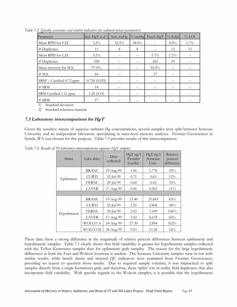
Table 7.2. Quality assurance and control indicators for sediment-phase parameters. Parameter Sed. HgT (s.d.1) Sed. meHg % meHg Perch HgT % Solid % LOI Mean RPD for F.D. 3.2% 32.5% 34.8% -- 8.0% 1.7% # Duplicates 13 8 8 -- 13 13 Mean RPD for L.D. 3.2% -- -- 5.7% 1.1% -- # Duplicates 328 -- -- 265 19 -- Mean recovery for M.S. 97.0% -- -- 92.9% -- --
# M.S. 64 -- -- 37 -- --
SRM2 – Certified 0.72 ppm 0.730 (0.029) -- -- -- -- --
# SRM 14 -- -- -- -- --
SRM Certified 1.12 ppm 1.20 (0.19) -- -- -- -- --
# SRM 17 -- -- -- -- -- 1) Standard deviation 2) Standard reference material
7.3 Laboratory intercomparison for HgT Given the sensitive nature of aqueous ambient Hg concentrations, several samples were split between Syracuse University and an independent laboratory specializing in trace-level mercury analyses. Frontier Geosciences in Seattle, WA was chosen for this purpose. Table 7.3 provides results of this intercomparison. Table 7.3. Results of 10 laboratory intercomparison aqueous HgT samples.
Strata Lake abbr. Date collected
HgT ng/l Frontier GeoSci.
HgT ng/l Syracuse
Univ.
Relative percent
difference
BRANC 19-Aug-99 1.96 1.776 10% CURTI 22-Jul-99 0.71 0.63 12% FERNL 29-Jul-99 0.60 0.43 33%
Epilimnion
LAVER 17-Aug-99 0.56 0.501 11%
BRANC 19-Aug-99 13.40 25.843 63% CURTI 22-Jul-99 1.55 2.808 58% FERNL 29-Jul-99 2.43 7.699 104% LAVER 17-Aug-99 3.52 6.678 62%
WOLCO A 24-Aug-99 27.30 2.894 162%
Hypolimnion
WOLCO D 24-Aug-99 9.53 11.24 16% These data show a strong difference in the magnitude of relative percent differences between epilimnetic and hypolimnetic samples. Table 7.1 clearly shows that field variability is greater for hypolimnetic samples collected with the Teflon Kemmerer sampler than for epilimnetic grab samples. The reason for the large hypolimnetic differences at both the Fern and Wolcott locations is unclear. The Syracuse University samples were re-run with similar results, while bench sheets and internal QC indicators were examined from Frontier Geosciences, providing no reason to question those results. Due to required sample volumes, it was impractical to split samples directly from a single Kemmerer grab, and therefore, these ‘splits’ wre in reality field duplicates, that also incorporate field variability. With specific regards to the Wolcott samples, it is possible that the hypolimnetic
Assessment of Mercury in Waters, Sediments, and Biota of VT and NH Lakes Project. Draft Final Report. Page 41

Assessment of Mercury in Waters, Sediments, and Biota of VT and NH Lakes Project. Draft Final Report. Page 42
bottles samples were inadvertently switched (e.g. mislabeled). As we are not convinced this is the case, these data were retained in the dataset. 7.4 Problems Individual quality assurance problems (e.g. bad blanks, duplicates, or unanticipated results) were addressed throughout the course of the project, in accordance with the project QAPP. Details on individual problems were discussed in the quarterly progress reports submitted throughout the course of the project, and included items such as switched labels, poor blank values for standard parameters, and contamination of one of the laboratory acid baths. Three larger-scale problems were encountered, that merit mention here. The first involves high blank results for aqueous HgT concentrations processed through Teflon Kemmerer sampler. This is discussed in some detail in the quarterly progress reports. In summary, it was a common occurrence for ambient Kemmerer bottle samples to run lower than blanks collected using the Kemmerer sampler. We attributed this to the volume of available Hg-clean blank/rinse water, which was insufficient to completely clean the sampler prior to processing the actual sample. This was due to a limited availability of clean Teflon sampling bottles, and not to the water itself. That is, carryover contamination from ambient samples to Kemmerer blanks may not have been completely prevented given the limited (~200ml) quantity of blank water used to pre-rinse each sampler. Adequate samples rinsing was not a problem for the routine samples, owing to the large volume of available rinse water (i.e., the lake itself) during acquisition of the hypolimnetic samples. Thus, despite these blank anomoliess, the project team feels that the results for hypolimnetic samples are valid, and they have been retained in the database. The second problem involved poor sediment meHg results for samples collected in 1998. Indeed, the meHg analyses for the entire set of sediment samples collected during 1998 were compromised owing to what remain unknown factors. During that year, sediment samples were stored in zip-style bags from collection to analysis at Syracuse University. We believe that methylation continued or was enhanced by the anaerobic environment within the zip-bags, for, when analyzed, numerous meHg values ran far above published values, and even in one or two instances, in excess of HgT. This did not make sense. The project team verified these meHg results at independent laboratories (Dr. Robert Mason, University of MD), and the samples were re-run numerous times at Syracuse University with no improvement. Accordingly, we feel that the results for the 1998 meHg analyses were in gross error, and these results have not been incorporated into the project database. The unweighted and weighted means and confidence intervals reported in Table 6.4 do not represent the entire sample of VT and NH lakes. The final problem involved analysis of HgT in zooplankton. One of several zooplankton analytical batches yielded quality control measurements that were well out of limits for the LaRosa laboratory. Specifically, blank aliquots included in the run produced very high results (~0.2 ug/g), suggesting contamination within the reagents or DI water. Simultaneously, the spikes accompanying those samples yielded very low recoveries (41%); a finding at odds with the high blank results. The chemists, despite a relatively exhaustive investigation, were unable to uncover the root of the problem, which was not subsequently replicated. The source of the error was eventually tracked to the digestion procedure, but the exact cause remains unknown. Owing to extremely limited quantities of sample, the analyses were not able to be re-run, and that single run of seven samples was lost.

Assessment of Mercury in Waters, Sediments, and Biota of VT and NH Lakes Project. Draft Final Report. Page 43
r
f
8.0 Analysis of the p oject data Numerous analyses have been performed using these project data. They include: a statistical age-adjustment of mean perch fillet Hg concentrations for each study lake; an estimation of the cumulative frequency distributions for all Hg parameters measures by the study; preparation of plots of various Hg measurements using GIS to identify the existence of geographic patterns; a formal statistical evaluation of project design factors; an evaluation of inter-annual data variability; an investigation of the effect of trophic status on Hg in waters and sediments; calculation of bioconcentration and bioaccumulation factors; an examination of univariate correlations between physicochemical and Hg variables; an estimation of principal components of physicochemical factors,and estimation of correlations of these factors to Hg variables; an evaluation of the role of land-use on Hg in fish tissue; and finally, estimation of linear discriminant functions to predict tissue Hg levels in fillets given physico-chemical data. Results of some of these analyses were recently published by Kamman et al. (2004). 8.1 Calculation o age-adjusted yellow perch fillet means for each study lake Yellow perch tissue HgT is known to vary both with fish size and fish age (Driscoll et al., 1994; Gilmour and Reidel, 2000; Carter et al., 2001). Both the length and age adjustment models were highly significant, with length and age explaining 31.6% and 19.1% of the total variance in inverse-root tissue HgT concentration across the lakes, respectively (length: F =57.44, p<0.001, d.f.=214, 17; age: F=7.29, p<0.001, d.f.=109, 122). A clean 1:1 relationship in age vs. length adjusted HgT tissue concentration existed for most lakes, although several outliers were apparent (Figure 8.1). Of these outliers, lakes falling well above the 1:1 relationship (Hardwood, Somerset, Suncook, and Wolcott) are all highly colored and acidic, while those falling below (Sunset-Brookfield and Sabin) are well buffered and pH circumneutral. Lakes with low pH and high DOC are commonly those with more elevated fish-tissue Hg concentrations (Mierle and Ingram, 1991; Driscoll et al., 1994; Carter et al., 2001, Kamman et al., 2004). Therefore, although the length-adjustment accounted for more overall variance than age, the age-adjusted concentrations were interpreted in this instance to more accurately estimate individual lake mean tissue concentrations. Mean muscle tissue HgT concentrations (inverse-root transformed), adjusted to the average age 4.6 year fish (the overall mean age, accounting for variance across study lakes) were retained for further analysis. These values were back-transformed to units of µg g-1 for discussion and plotting purposes only.
LS Mean Filet Yellow Perch HgTug . g -1
Mean length = 21cm
0.0 0.1 0.2 0.3 0.4 0.5 0.6
LS M
ean
File
t Yel
low
Per
ch H
gTug
. g
-1
Mea
n ag
e =
4.6
yrs
0.0
0.1
0.2
0.3
0.4
0.5
0.6
0.7
0.8
Wolcott
Somerset
SabinSunset (Brkfld)
Hardwood
Suncook
Figure 8.1. Relationship between age and length-adjusted yellow perch muscle-tissue least squared mean HgT concentrations.

Assessment of Mercury in Waters, Sediments, and Biota of VT and NH Lakes Project. Draft Final Report. Page 44
8.2 GIS analyses Several water and sediment Hg parameters were plotted using Arcview GIS (ESRI Inc, v 3.1, 2000), to visually evaluate whether any patterns exist across the Vermont-New Hampshire landscape. Mean values of all sampling events, excluding blank samples, were used to generate these plots. Individual sample-lake values are displayed as their deviation from the grand mean for each parameter. Figure 8.2 displays the plots, which yield the following parameter-specific observations:
• Epilimnetic HgT: No discernable patterns in deviations from the mean are apparent. • Epilimnetic meHg: A greater proportion of lakes displaying elevated meHg concentrations occur in
New Hampshire. There is also a cluster of lakes showing elevated meHg in northeastern VT. • Hypolimnetic HgT: New Hampshire lakes display greater hypolimnetic HgT concentrations overall.
The highest hypolimnetic concentrations occur in the southern-most reaches of the study region. • Hypolimnetic meHg: Hypolimnetic meHg is elevated in south-central and southeastern New
Hampshire. • Sediment HgT: No discernable pattern is apparent. • Sediment MeHg: No discernable pattern is apparent, save that a cluster of lakes showing elevated
sediment MeHg exists in south-central New Hampshire. • Yellow perch, whole-fish composites, < 15cm: No pattern is apparent in the geographic distribution of
prey-sized yellow perch composite whole-body HgT or meHg. However, most southeastern New Hampshire lakes do appear to have elevated HgT and MeHg levels in prey-sized yellow perch
• Yellow Perch, fillet age-adjusted mean HgT: Two patterns are apparent. First, tissue HgT means are most variable in north-eastern Vermont. Second, there exists a cluster of lakes with elevated tissue HgT concentrations in southern New Hampshire. This ‘hotspot’ coincides with that noted for sediment meHg.
• Yellow perch fillets, exceedences of the 0.3 µg g-1 meHg standard: Tissue criterion exceedences are apparent in the southern New Hampshire hotspot, in three central New Hampshire lakes, in one southern Vermont lake, and in two northern Vermont lakes.

Yellow Perch Fillet HgTmean = 239 ng/g w.w.
age 4.6 fish
### ##
##
# ####
####
## # ##
#
#
####
# ### #
## ##
##### ####
##
## ### ###
# ######
####
### # ###
##
## #
#
##
#
####
# ##### # ## ## ## ## ##
# ## #### ####
## #
### ### # ### ### ##
# # ######
####
### # ### # #
####
# ##
####
#
### # ## ##
# ## ##### # ## # ## ## ## # ##
## ## #### ####
## #
### ### # ### ### ##
# # ######
####
### # ### # #
####
# ##
####
#
### # ## ##
# ## ##### # ## # ## ## ## # ##
## ## #### ####
##
### ## ####
###
#
#### # #
##
#
#
## ##
# # ##### #
# #
### #
##
### ## ####
###
#
#### # #
##
#
#
## ##
# # ##### #
# #
### #
### ##
##
# ####
####
## # ##
#
#
####
# ### #
## ##
##### ####
## #
### ### # ### ### ##
# # ######
####
### # ### # #
####
# ##
####
#
### # ## ##
# ## ##### # ## # ## ## ## # ##
## ## #### ####
Epilimnetic HgTmean = 1.78 ng/l
Epilimnetic meHgmean = 0.299 ng/l
Hypolimnetic HgTmean = 11.52 ng/l
Hypolimnetic meHgmean = 0.829 ng/l
Prey Yellow Perch, HgTmean = 95 ng/g w.w.
Prey Yellow Perch, meHgmean = 91 ng/g w.w. Sediment HgT
mean = 210 ng/g d.w.
Sediment meHgmean = 4 ng/g d.w.
## #
### ### # ### ### ##
# # ######
####
### # ### # #
####
# ##
####
#
### # ## ##
# ## ##### # ## # ## ## ## # ##
## ## #### ####
### ##
##
# ####
####
## # ##
#
#
####
# ### #
## ##
##### ####
Yellow Perch Fillets, EPA Tissue MeHg Criterion Exceedences
age 4.6 fish (red >0.30 ug/g HgT, blue < 0.30 ug/g HgT)
Legend# -2 - -1 Std. Dev.# -1 - 0 Std. Dev.# 0 - 1 Std. Dev.# 1 - 2 Std. Dev.# 2 - 3 Std. Dev.# > 3 Std. Dev.
Figure 8.2. Mercury in sediment, water, and yellow perch tissues of lakes sampled in conjunction with this project. Values are expressed as standard deviations from the mean. Weighted mean concentrations for each parameter are shown.
Assessment of Mercury in Waters, Sediments, and Biota of VT and NH Lakes Project. Draft Final Report. Page 45
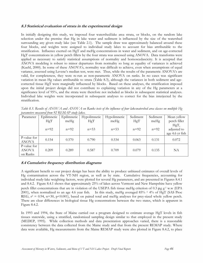
8.3 Statistical evaluation of strata in the experimental design In initially designing this study, we imposed four watershed:lake area strata, or blocks, on the random lake selection under the premise that Hg in lake water and sediment is influenced by the size of the watershed surrounding any given study lake (see Table 2.1). The sample draw was approximately balanced around these four blocks, and weights were assigned to individual study lakes to account for bias attributable to the stratification. Influence exerted on HgT and meHg concentrations in water and sediment, and on age-corrected HgT concentrations in yellow perch fillets by the four strata was assessed using ANOVA. Data transforms were applied as necessary to satisfy statistical assumptions of normality and homoscedascicity. It is accepted that ANOVA modeling is robust to minor departures from normality so long as equality of variances is achieved (Kuehl, 2000). In some of these ANOVA’s, normality was difficult to achieve, even when assumptions of equal variance, assessed using Levene’s median test, were met. Thus, while the results of the parametric ANOVA’s are valid, for completeness, they were re-run as non-parametric ANOVA on ranks. In no cases was significant variation in mean Hg values attributable to strata (Table 8.3), although the variances in both sediment and age-corrected tissue HgT were marginally influenced by blocks. Based on these analyses, the stratification imposed upon the initial project design did not contribute to explaining variation in any of the Hg parameters at a significance level of 95%, and the strata were therefore not included as blocks in subsequent statistical analyses. Individual lake weights were incorporated in subsequent analyses to correct for the bias interjected by the stratification. Table 8.3. Results of ANOVA and ANOVA on Ranks tests of the influence of four lake:watershed area classes on multiple Hg parameters measured from 92 REMAP study lakes. Parameter Epilimnetic
HgT
n=92
Epilimnetic meHg
n=92
Hypolimnetic HgT
n=53
Hypolimnetic meHg
n=53
Sediment HgT
n=92
Sediment meHg
n=92
Mean yellow perch fillet
HgT, adjusted to
age 4.6 yr fishP-value for ANOVA 0.154 0.570 0.790 0.534 0.063 0.131 0.072
P-value for ANOVA on Ranks
0.209 0.289 0.587 0.709 0.079 0.135 NA
8.4 Cumulative frequency distribution diagrams A significant benefit to our project design has been the ability to produce unbiased estimates of overall levels of Hg contamination across the VT-NH region, as well as by state. Cumulative frequencies, accounting for individual study-lake weighting factors, were plotted for several Hg parameters, and are presented in Figures 8.4.1 and 8.4.2. Figure 8.4.1 shows that approximately 25% of lakes across Vermont and New Hampshire have yellow perch fillet concentrations that are in violation of the USEPA fish tissue meHg criterion of 0.3 µg g-1 w.w (EPA 2001), when normalized to an age 4.6 year fish. In this study, meHg averaged 85% ± 4% of HgT (SAS Proc REG, r2 = 0.94, n=30, p<0.001), based on paired total and meHg analyses for prey-sized whole yellow perch. There are clear differences in biological tissue Hg concentrations between the two states, which is apparent in Figure 8.4.2. In 1993 and 1994, the State of Maine carried out a program designed to estimate average HgT levels in fish tissues statewide, using a stratified, randomized sampling design similar to that employed in the present study (MEDEP, 1995). While collection methods and data presentation approaches varied, there is a reasonable consistency between the data collected from the Maine study and that from the present REMAP study. Where data were available, Hg measurements from the Maine REMAP study were also plotted in Figure 8.4.2, to place
Assessment of Mercury in Waters, Sediments, and Biota of VT and NH Lakes Project. Draft Final Report. Page 46
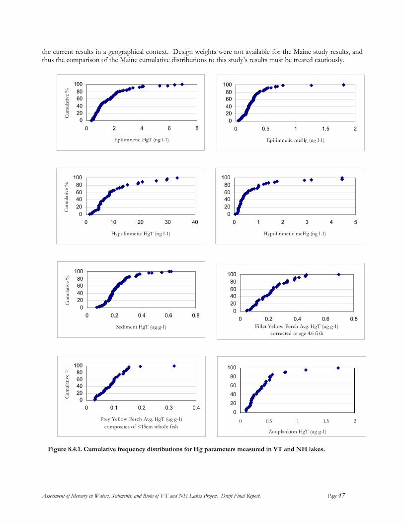
the current results in a geographical context. Design weights were not available for the Maine study results, and thus the comparison of the Maine cumulative distributions to this study’s results must be treated cautiously.
020406080
100
0 0.2 0.4 0.6 0.8Fillet Yellow Perch Avg. HgT (ug g-1)
corrected to age 4.6 fish
020406080
100
0 0.2 0.4 0.6 0.8
Sediment HgT (ug g-1)
Cum
ulat
ive
%
020406080
100
0 2 4 6 8
Epilimnetic HgT (ng l-1)
Cum
ulat
ive
%
020406080
100
0 10 20 30 40
Hypolimnetic HgT (ng l-1)
Cum
ulat
ive
%
020406080
100
0 0.5 1 1.5 2
Epilimnetic meHg (ng l-1)
020406080
100
0 1 2 3 4 5
Hypolimnetic meHg (ng l-1)
020406080
100
0 0.1 0.2 0.3 0.4
Prey Yellow Perch Avg. HgT (ug g-1)composites of <15cm whole fish
Cum
ulat
ive
%
020406080
100
0 0.5 1 1.5 2
Zooplankton HgT (ug g-1)
Figure 8.4.1. Cumulative frequency distributions for Hg parameters measured in VT and NH lakes.
Assessment of Mercury in Waters, Sediments, and Biota of VT and NH Lakes Project. Draft Final Report. Page 47

020406080
100
0 0.2 0.4 0.6 0.8 1Yellow Perch Avg. HgT (ug g-1)
corrected to age 4.6 fish
Cum
ulat
ive
%
0
20
40
60
80
100
0 0.2 0.4 0.6 0.8Sediment HgT (ug g-1)
Cum
ulat
ive
%
New Hampshire
Vermont
Maine
020406080
100
0 0.5 1 1.5 2
Epilimnetic meHg (ng l-1)
Cum
ulat
ive
%
02040
6080
100
0 2 4 6 8Epilimnetic HgT (ng l-1)
Cum
ulat
ive
%New Hampshire
Vermont
020406080
100
0 1 2 3 4 5
Hypolimnetic meHg (ng l-1)
Cum
ulat
ive
%
020406080
100
0 10 20 30 40
Hypolimnetic HgT (ng/L)
Cum
ulat
ive
%
0
20
40
60
80
100
0 0.5 1 1.5 2
Zooplankton HgT (ug g-1.)
Cum
ulat
ive
%
020406080
100
0 0.1 0.2 0.3 0.4
Prey Yellow Perch Avg. HgT (ug g-1)composites of <15cm whole fish
Cum
ulat
ive
%
Figure 8.4.2. Cumulative frequency distributions for Hg parameters, by State.
Assessment of Mercury in Waters, Sediments, and Biota of VT and NH Lakes Project. Draft Final Report. Page 48

8.5 Evaluation of inter-annual variability and replicate sampling Since the sampling effort for this study spanned 1998 to 2000, an assessment of inter-annual variability was performed to determine whether significant variation in water and sediment chemistry could be attributed either to the years in which the samples were collected (1998 vs. 1999), or to sample replication. This analysis was conducted using multivariate analysis of variance (MANOVA) to account for simultaneous covariance among the numerous parameters measured. Separate MANOVA were performed on epilimnetic and hypolimnetic water chemistry, and on sediment chemistry. Where MANOVA indicated a significant difference attributable to year, follow-up univariate ANOVA was used to determine which parameters influenced this variation. The 1998 vs. 1999 statistical model evaluated the null hypothesis that no linear combination existed that could produce a significant difference in the mean multivariate water or sediment chemistry observation, between years. For the replication analysis, the statistical model evaluated the null hypothesis that no linear combination existed that could produce a significant difference in the mean multivariate water or sediment chemistry observation, while accounting for the expected variation due to individual lakes. For epilimnetic samples, a statistically significant difference in water chemistry was evident between years (Table 8.5). Follow-up ANOVA indicated that log-HgT was the only parameter which varied significantly between 1998 and 1999. For hypolimnetic water chemistry and sediment chemistry, no significant differences between years were noted. The analysis of replicates (collected in 2000) yielded identical results (Table 8.5); differences in replicates were apparently confounded with differences attributable to year. Table 8.5. Results of MANOVA and follow-up ANOVA analyses of inter-annual variability and replicate sampling. P-values are provided only where there is significant variation across years or between replicates (ns: not significant at the 95% probability level).
Epilimnetic water
Hypolimnetic water
Sediment Epilimnetic water
Hypolimnetic water
Sediment
Comparison 1998 to 1999
Comparison replicate measurements, 1998 to 2000
Wilks’ Λ, F statistic p-value
0.520, 10.26, <0.001
0.860, 0.97, ns
0.970, 0.99, ns
0.326, 4.39, 0.005
0.444, 2.00, ns
0.809, 1.80, ns
Follow-up univariate ANOVA p-values for transformed variables Secchi transparency
ns ns
ANC ns ns Chlorides ns ns SO4 ns ns DOC ns ns Total color ns ns meHg ns ns HgT <0.001 0.002 Sediment HgT -- -- Loss on Ignition
-- --
Solid % -- -- In order to test that observed differences in HgT between replicate samples was indeed confounded with that variation attributable to year, data from each year of sampling (1998, 1999, and 2000) were plotted as separate groups (Figure 8.5.1). Although no statistical comparisons are possible because the lakes visited in 2000 were not randomly selected, it is clear from this plot that any differences between the mean HgT concentrations from 1998 through 2000 are obscured by the large variance exhibited in 1998. Two-way ANOVA indicates that epilimnetic HgT varied with year and with state (F = 30.37, p<0.001, d.f.=3, 94). Year was highly significant (p<0.001), but a significant interaction also existed between year and state
Assessment of Mercury in Waters, Sediments, and Biota of VT and NH Lakes Project. Draft Final Report. Page 49

(p=0.028), in that New Hampshire lakes appeared to display higher concentrations than did Vermont lakes in 1998 (Figure 8.5.2). However, no statistical difference in the mean HgT concentrations between the states existed, once the effect of year was accounted for. In 1998, mean epilimnetic HgT 1.46 ng l-1 greater than the 1999 mean. There are several potential reasons for the observed differences in HgT concentration means across the two main sampling years. Chief among these are laboratory error, sampling error, and real differences driven by natural factors such as weather. Lorey (2002) discusses the ramifications of a change in laboratory location at Syracuse University that occurred between 1998 and 1999. The only quantifiable change in analytical results was a reduction in mean blank concentrations. Sampling for this project was performed by two separate teams, one from VT, and the other from New Hampshire. If a sampling problem were to blame for the observed differences in HgT concentrations across years, it would be expected that the 1998 results from one state would be significantly different from the other. The analysis presented above only marginally supports this inference for 1998, and not at all for 1999 (difference between mean 1998 VT and NH samples = 0.33 ± 0.37 ng l-1, p = 0.079). Moreover, no significant differences were detected in any other parameters, including hypolimnetic HgT and meHg, and sediment HgT. The most likely explanation for the differences in epilimnetic HgT concentrations observed between 1998 and 1999 is related to rainfall. Mean monthly rainfall totals from Burlington, VT (annual mean ~36 inches) and Concord, NH (annual mean ~50 inches) in relation to long-term averages for the period 1991 to 2001 show very different patterns (Figure 8.5.3). In 1998, rainfall for June through September, measured at Burlington, VT was 232% of the long-term average; at Concord, N.H., it was 117 % of the long-term average (National Weather Service, 2002). In 1999 and 2000, rainfall averages were at or below long-term means. A very significant proportion of annual wet Hg deposition can result from a very few storms of high intensity, with peak deposition
in the spring or summer period (Burke et al., 1995; Hoyer et al., 1995; Shanley et al., 1999). The degree to which this can translate to increased observed concentrations in lake waters is unclear. Nonetheless, the summer of 1998 produced four record single-day rainfall events recorded at the Burlington, VT weather station between May 31 and August 30. Two record storms passed over Boston in 1998, including one 5.67 inch, 24 hour deluge. Obviously, actual precipitation conditions in close proximity to the study lakes will directly affect in-lake HgT concentrations, and such precipitation data are unavailable as of this writing. It seems clear, however,
1998
-NH
1998
-VT
1999
-NH
1999
-VT
2000
-NH re
sample
s
2000
-VT re
sample
s
HgT
(ng
l-1)
0
2
4
6
8
Figure 8.5.1. Tukey box-plots of epilimnetic HgT concentration byyear and state, for samples collected during 1998, 1999, and 2000.
1998-NH 1998-VT 1999-NH 1999-VT
HgT
ng
l-1
(+/-
95%
CI)
0.0
0.5
1.0
1.5
2.0
2.5
3.0
3.5
4.0
Figure 8.5.2. Mean concentrations of HgT in epilimneticwaters(and 95% confidence intervals) by year and State. Plottedvalues are back-transformed least-squares estimates.
Assessment of Mercury in Waters, Sediments, and Biota of VT and NH Lakes Project. Draft Final Report. Page 50

that 1998 was a particularly wet year, and abnormally so in Vermont. This may partially explain the elevated HgT observations in our study lakes in 1998. 8.6 Evaluation of Hg variation in relation to trophic status Understanding the degree to which Hg varies in lakes in response to trophic gradients can be useful in determining where trophic transfer of Hg may be enhanced or dampened. Dystrophic lakes are well understood to display elevated tissue Hg concentrations. Lakes
of increased trophic status are those that are expected to have experienced enhanced watershed disturbance, and thus receive greater Hg loadings from the watershed (Shanley et al., 1999; Mason and Sullivan, 1998), producing increased in-lake and sediment Hg burdens. Pickhardt et. al. (2002) convincingly demonstrated that Hg is biodiluted in waters where phytoplankton densities are high. This so-named ‘bloom dilution’ results from algal density-dependant incorporation of the bioavailable Hg pool into the phytoplankton. When algal densities are higher, Hg per unit of algal density will be lower, the result being that the available Hg pool is spread across a larger primary aquatic production base. Pickhardt et al. show that biodilution of Hg by high densities of phytoplankton results in reduced HgT concentrations in Ceriodaphnia sp., suggesting that bioaccumulation at higher trophic levels will be muted, a phenomenon noted by Chen et al. (2000). The present dataset provides a good means to independently evaluate the hypothesis that mean fish tissue Hg concentrations will be reduced in lakes of elevated trophic status.
1990 1992 1994 1996 1998 2000 2002
Perc
ent o
f lon
g-te
rm m
ean
June
-Sep
. pre
cipi
tatio
n
406080
100120140160180200220240260
Burlington VT Concord NH
Figure 8.5.3. 1991-2001 mean June through September precipitation atBurlington, VT and Concord, N.H., expressed as percent of the long-term June-September mean. Period of record: Burlington, 119 years;Concord, 82 years.
To investigate variation in Hg measures with trophic state, lakes were allocated into one of four groups based on total phosphorus concentrations, DOC, and color, as initially described by VTDEC (1996). Trophic data were acquired from the VTDEC and NHDES respective Lake Inventory Databases, and were based on each State’s long-term monitoring and assessment programs. The four trophic classes were oligotrophic (<8 µg l-1 total phosphorus), mesotrophic (8-16 µg l-1 total phosphorus), eutrophic (>16 µg l-1 total phosphorus), and dystrophic (TC >50 PtCo units and/or DOC > 4 mg l-1). A series of ANOVA analyses was employed to evaluate the hypothesis that lake trophic status influences aqueous, sediment, and tissue Hg concentrations. Sample weights were incorporated into the analyses, and post-test pairwise comparisons were adjusted to an overall experiment-wise error rate of 5% using the method of Scheffe (SAS Institute, 2002). ANOVA showed that epilimnetic HgT and meHg, and hypolimnetic meHg concentrations varied significantly with trophic state, while hypolimnetic HgT concentrations did not. Neither sediment HgT nor meHg showed significant differences, but HgT concentrations in perch tissue were highly significantly different between trophic states. Scheffé contrasts showed that epilimnetic HgT concentrations (Figure 8.6A) were elevated in dystrophic lakes relative to mesotrophic and oligotrophic lakes (p=0.017 and 0.047 respectively), and in eutrophic lakes relative to mesotrophic lakes (p = 0.021). Epilimnetic meHg concentrations (Figure 8.6B) in dystrophic and eutrophic lakes were marginally elevated relative only to oligotrophic lakes (p = 0.097 and 0.089 respectively). Hypolimnetic meHg concentrations(Figure 8.6C) in eutrophic lakes were marginally elevated relative to mesotrophic lakes (p=0.063). Age-adjusted yellow perch Hg tissue levels (Figure 8.6D) were significantly elevated
Assessment of Mercury in Waters, Sediments, and Biota of VT and NH Lakes Project. Draft Final Report. Page 51

Epi
limne
tic H
gT (n
g l-1
)
0.5
1.0
1.5
2.0
2.5
3.0
Epi
limne
tic m
eHg
(ng
l-1)
0.10
0.15
0.20
0.25
0.30
0.35
0.40
0.45
in dystrophic lakes relative mesotrophic lakes (p=0.012), and significantly lower in eutrophic lakes relative to all other lake types (p<0.005). These data also indicate that, on average, age 4.6 year perch from dystrophic lakes have tissue levels that were greater by 0.218 µg g-1 than the mean for all other lake types (p <0.001).
Trophic State
D E M O
Hyp
olim
netic
meH
g (n
g l-1
)
0.0
0.2
0.4
0.6
0.8
1.0
1.2
1.4
Trophic State
D E M O
Mea
n ag
e 4.
6yr
Yell
ow p
erch
fille
t (ug
g-1
w.w
.)
0.0
0.1
0.2
0.3
0.4
0.5
0.6
A B
C D
p=0.007 p=0.0193
p=0.0173 p=0.0001
Figure 8.6. Back-transformed least-squares means and 95% confidence intervals for four mercuryparameters in relation to four lake trophic states. D: dystrophic; E: eutrophic; M: mesotrophic; O:oligotrophic. P-values from ANOVA. Underlined means were not significantly different based on Scheffécontrasts.
These findings are noteworthy in relation to currently available literature. Elevated HgT concentrations in dystrophic waters is not surprising, and is well documented (e.g., Mierle and Ingram, 1991; Driscoll et al., 1994; Ullrich et al., 2001). Equally unsurprising and well documented (e.g., Driscoll et al., 1994; USEPA 1997; Carter et al., 2001) is the fact that yellow perch from dystrophic lakes also show elevated mercury. Somewhat more interesting is the elevated HgT concentrations observable in epilimnetic waters of eutrophic lakes relative to lakes of lower trophic status, a finding which partially supports the hypothesis that lakes with disturbed watersheds incur greater HgT loading. Of greatest interest in this analysis is the finding that tissue HgT concentrations were quite low in eutrophic lakes (mean = 0.056 µg g-1). Although this finding must be treated cautiously owing to a small sample size (n=3 for eutrophic lakes with tissue data in this dataset), the finding directly supports the hypothesis of algal biodilution, and is consistent with other studies showing low tissue HgT in fishes from eutrophic lakes (Pickhardt et al. 2002). Further evaluation of tissue Hg data in relation to lake trophic status could be accomplished using myriad state fish tissue contamination databases, and presents a fruitful avenue for additional inquiry.
Assessment of Mercury in Waters, Sediments, and Biota of VT and NH Lakes Project. Draft Final Report. Page 52
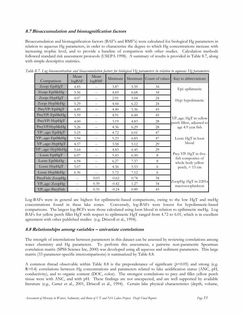
8.7 Bioaccumulation and biomagnification factors Bioaccumulation and biomagnification factors (BAF’s and BMF’s) were calculated for biological Hg parameters in relation to aqueous Hg parameters, in order to characterize the degree to which Hg concentrations increase with increasing trophic level, and to provide a baseline of comparison with other studies. Calculation methods followed standard risk assessment protocols (USEPA 1998). A summary of results is provided in Table 8.7, along with simple descriptive statistics. Table 8.7. Log bioconcentration and bioaccumulation factors for biological Hg parameters in relation to aqueous Hg parameters.
Comparison Mean
logBAF Mean
logBMF Minimum Maximum Count of values Key to abbreviations
Zoop: EpiHgT 4.85 -- 3.87 5.59 34 Zoop: EpiMeHg 5.56 -- 4.69 6.68 34
Epi: epilimnetic
Zoop: HypHgT 4.07 -- 2.91 5.04 24 Zoop: HypMeHg 5.29 -- 4.44 6.22 24
Hyp: hypolimnetic
PreyYP: EpiHgT 4.89 -- 4.40 5.36 45 PreyYP: EpiMeHg 5.59 -- 4.91 6.44 45 PreyYP: HypHgT 4.00 -- 3.19 4.83 28 PreyYP:HypMeHg 5.26 -- 4.36 6.29 28 YP _age: EpiHgT 5.25 -- 4.72 6.01 47
YP_age: HgT in yellow perch fillets, adjusted to
age 4.9 year fish
YP _age: EpiMeHg 5.94 -- 5.23 6.85 47 YP _age: HypHgT 4.37 -- 3.58 5.12 29
Loon: HgT in loon blood
YP _age: HypMeHg 5.64 -- 4.83 6.45 29 Loon: EpiHgT 6.07 -- 5.43 6.50 8
Loon: EpiMeHg 6.94 -- 6.27 7.37 8 Loon: HypHgT 5.07 -- 4.36 5.53 6
Loon: HypMeHg 6.36 -- 5.72 7.12 6
Prey YP: HgT in five-fish composites of whole body yellow
perch, < 15 cm
PreyFish: ZoopHg -- 0.03 -0.62 0.78 34 YP_age: ZoopHg -- 0.39 -0.42 1.27 34 YP_age: PreyFish -- 0.35 -0.24 0.89 45
ZoopHg: HgT in ≥201umacrozooplankton
Log-BAFs were in general are highest for epilimnetic-based comparisons, owing to the low HgT and meHg concentrations found in these lake zones. Conversely, log-BAFs were lowest for hypolimnetic-based comparisons. The largest log-BCFs were those calculated using loon blood in relation to epilimnetic meHg. Log BAFs for yellow perch fillet HgT with respect to epilimnetic HgT ranged from 4.72 to 6.01, which is in excellent agreement with other published studies (e.g. Driscoll et al., 1994). 8.8 Relationships among variables – univariate correlations The strength of interrelations between parameters in this dataset can be assessed by reviewing correlations among water chemistry and Hg parameters. To perform this assessment, a pairwise non-parametric Spearman correlation matrix (SPSS Science Inc, 2000) was developed using all aqueous and sediment parameters. This large matrix (33 parameter-specific intercomparisons) is summarized by Table 8.8. A common thread observable within Table 8.8 is the preponderance of significant (p<0.05) and strong (e.g. R>0.4) correlations between Hg concentrations and parameters related to lake acidification status (ANC, pH, conductivity), and to organic content (DOC, color). The strongest correlations to prey and fillet yellow perch tissue were with ANC, and with pH. These findings are not unexpected, and are well supported by available literature (e.g., Carter et al., 2001, Driscoll et al., 1994). Certain lake physical characteristics (depth, volume,
Assessment of Mercury in Waters, Sediments, and Biota of VT and NH Lakes Project. Draft Final Report. Page 53

flushing rate) correlated to several Hg parameters, indicating that hydrology influenced: epilimnetic and hypolimnetic HgT concentrations; methylation; and, sediment HgT sequestration. Flushing rate also has a minor influence over perch HgT concentrations. Table 8.8. Summary of significant (p≤0.05) Spearman correlation coefficients among water chemistry variables in relation to Hg parameters. Parameter names in bold indicate Spearman R values of >0.4, names in italic bold indicate values >0.7, names in strikeout are expected mathematical artifacts.
EpiMe HypMe EpiHgT HypHgT SHgT SmeHg ZoopHg PreyYP YP_age EpiMe% HypMe% SedMe%
Para
met
ers w
ith si
gnifi
cant
Spe
arm
an R
’s. EpiANC
EpiSO4 EpiDOC HypDOC EpiTC HypTC MinTemp Mean pH Mean Z Vol_m3 FlushRate
HypNOx HypSO4 EpiDOC HypDOC EpiTC HypTC Mean Z TP EpiMe
EpiANC HypANC EpiSO4 HypSO4 EpiDOC HypDOC EpiTC HypH2S Mean pH Mean cond WA:LA Mean Z Vol_m3 FlushRate TP EpiMe HypMe
EpiANC HypANC EpiNOx HypNOx HypDOC Mean pH HypMe
EpiANC HypANC EpiCl- Mean pH MeanCond WA:LA
SHgT MeanCond EpiANC HypANC EpiSO4 EpiDOC HypDOC Min Temp Mean pH MeanCondFlushRate
EpiHgT
EpiANC HypANC EpiSO4 HypSO4 EpiDOC HypDOC Mean pH MeanCond FlushRate
EpiHgT PreyYP
EpiCl- HypCl- EpiTC EpiMe EpiHgT
HypTC Min DO TP HypMe
FlushRate
EpiMe EpiMe
HypHgT SHgT SmeHg
HypANCHypHgT SmeHg PreyYP
Abbreviations: Epi: epilimnetic; Hyp: hypolimnetic; S: sediment; Me: meHg; ZoopHg: HgT in zooplankton; PreyYP: HgT in whole body-composites of <15 cm yellow perch; YP_age: age-adjusted yellow perch fillet (average age 4.9 years) HgT means; Me%: % of HgT as meHg; ANC: acid neutralizing capacity; DOC: dissolved organic carbon; TC: total color; TP: total phosphorus; DO: dissolved oxygen; Cond: conductivity; WA:LA: ratio of watershed:lake area, Z: depth.
8.9 Principal components analysis - accounting for covariance among parameters While a univariate correlation matrix is useful to look at individual relationships between parameters, it is clear from Table 8.8 that numerous parameters are simultaneously influencing Hg fate in the study lakes. Moreover, a 33 parameter correlation matrix is sufficiently large so as to yield spurious correlations. Accordingly, principal components analysis was used to reduce the dataset, to account for simultaneous covariance among parameters that jointly influence concentrations of HgT, meHg, sediment HgT, and tissue Hg, and to control for the occurrence of spurious correlations. All non-Hg water chemistry variables were entered into two separate datasets describing mean epilimnetic and hypolimnetic water chemistry for each lake, accounting for all available sampling events. For each dataset, principal components were extracted and reported from the correlation matrix of untransformed variables (Rencher, 1995), using SAS Proc Princomp (SAS Institute, 2002). It was decided a-priori that the first three components would be retained. Component loadings for the first three axes from each dataset were calculated using SAS Proc Corr (SAS Institute 2002). Extraction of principal components requires a complete dataset. To avoid excessive data loss, missing values for several individual cell values were determined as follows: 1) use of the mean of the remaining parameter values (one SO4 and one Cl- datapoint for Childs Bog, NH); 2) use of the relationship between total color and DOC (p<0.001, r2 = 0.560, one total color datapoint for Noyes Pond, VT) 3) use of available pH and conductivity data from NHDES Lake Inventory Database (15 datapoints) The resultant epilimnetic dataset was comprised of 91 records, containing 11 water chemistry variables. The first three principal components captured 66.5 percent of the total dataset variation. The hypolimnetic dataset was
Assessment of Mercury in Waters, Sediments, and Biota of VT and NH Lakes Project. Draft Final Report. Page 54
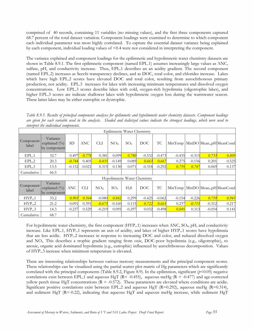
comprised of 40 records, containing 11 variables (no missing values), and the first three components captured 68.7 percent of the total dataset variation. Component loadings were examined to determine to which component each individual parameter was most highly correlated. To capture the essential dataset variance being explained by each component, individual loading values of <0.4 were not considered in interpreting the component. The variance explained and component loadings for the epilimnetic and hypolimnetic water chemistry datasets are shown in Table 8.9.1. The first epilimnetic component (named EPI_1) assumes increasingly large values as ANC, sulfate, pH, and conductivity increase. Thus, EPI_1 describes an an acidity gradient. The second component (named EPI_2) increases as Secchi transparency declines, and as DOC, total color, and chlorides increase. Lakes which have high EPI_2 scores have elevated DOC and total color, resulting from autochthonous primary production, not acidity. EPI_3 increases for lakes with increasing minimum temperatures and dissolved oxygen concentrations. Low EPI_3 scores describe lakes with cold, oxygen-rich hypolimnia (oligotrophic lakes), and higher EPI_3 scores are indicate shallower lakes with hypolimnetic oxygen loss during the warmwater season. These latter lakes may be either eutrophic or dystrophic. Table 8.9.1. Results of principal components analyses for epilimnetic and hypolimnetic water chemistry datasets. Component loadings are given for each variable used in the analysis. Shaded and italicized values indicate the strongest loadings, which were used to interpret the individual components.
Epilimnetic Water Chemistry
Component label
Variance explained (%) by component
SD ANC CLI NOX SO4 DOC TC MinTemp MinDO Mean_pH MeanCond
EPI_1 32.7 0.497 0.778 0.381 0.099 0.780 -0.532 -0.473 -0.435 -0.315 0.733 0.809EPI_2 20.3 -0.744 0.405 0.435 -0.149 0.089 0.663 0.667 0.275 -0.156 0.201 0.525EPI_3 13.5 -0.152 -0.021 0.315 0.130 0.071 -0.318 -0.292 0.759 0.747 0.069 0.137
Cumulative 66.5 Hypolimnetic Water Chemistry
Component label
Variance explained (%) by component
ANC CLI NOX SO4 H2S DOC TC MinTemp MinDO Mean_pH MeanCond
HYP_1 33.2 0.901 0.564 -0.080 0.842 0.299 -0.425 -0.062 -0.154 -0.226 0.759 0.941HYP_2 21.2 0.091 0.391 -0.673 -0.160 0.115 0.722 0.665 0.237 -0.715 -0.312 0.217HYP_3 14.3 -0.237 0.529 -0.219 0.095 -0.297 0.032 -0.498 0.849 0.313 -0.054 0.141
Cumulative 68.7 For hypolimnetic water chemistry, the first component (HYP_1) increases when ANC, SO4, pH, and conductivity increase. Like EPI_1, HYP_1 represents an axis of acidity, and lakes of higher HYP_1 scores have hypolimnia that are less acidic. HYP_2 increases in response to increasing DOC and color, and reduced dissolved oxygen and NOx. This describes a trophic gradient ranging from oxic, DOC-poor hypolimnia (e.g., oligotrophic), to anoxic, organic acid dominated hypolimnia (e.g., eutrophic) influenced by autochthonous decomposition. Values of HYP_3 increase when minimum temperature is elevated. There are interesting relationships between various mercury measurements and the principal component scores. These relationships can be visualized using the partial scatter plot matrix of Hg parameters which are significantly correlated with the principal components (Table 8.9.2, Figure 8.9). In the epilimnion, significant (p<0.05) negative correlations exist between EPI_1 and aqueous HgT (R= -0.455), aqueous meHg (R = -0.477) and age-corrected yellow perch tissue HgT concentrations (R = -0.572). These parameters are elevated where conditions are acidic. Significant positive correlations exist between EPI_2 and aqueous HgT (R=0.292), aqueous meHg (R=0.314), and sediment HgT (R=-0.22), indicating that aqueous HgT and aqueous meHg increase, while sediment HgT
Assessment of Mercury in Waters, Sediments, and Biota of VT and NH Lakes Project. Draft Final Report. Page 55
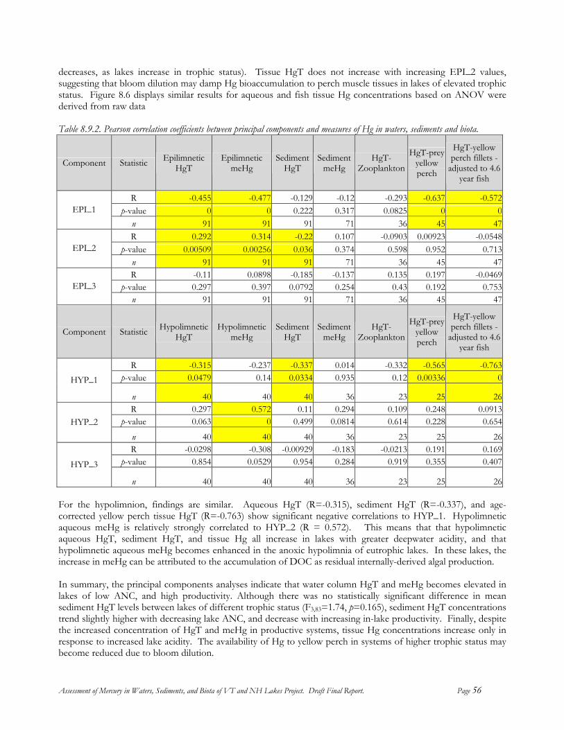
decreases, as lakes increase in trophic status). Tissue HgT does not increase with increasing EPI_2 values, suggesting that bloom dilution may damp Hg bioaccumulation to perch muscle tissues in lakes of elevated trophic status. Figure 8.6 displays similar results for aqueous and fish tissue Hg concentrations based on ANOV were derived from raw data Table 8.9.2. Pearson correlation coefficients between principal components and measures of Hg in waters, sediments and biota.
Component Statistic Epilimnetic HgT
Epilimnetic meHg
Sediment HgT
Sediment meHg
HgT-Zooplankton
HgT-prey yellow perch
HgT-yellow perch fillets -
adjusted to 4.6 year fish
R -0.455 -0.477 -0.129 -0.12 -0.293 -0.637 -0.572p-value 0 0 0.222 0.317 0.0825 0 0EPI_1
n 91 91 91 71 36 45 47R 0.292 0.314 -0.22 0.107 -0.0903 0.00923 -0.0548
p-value 0.00509 0.00256 0.036 0.374 0.598 0.952 0.713EPI_2 n 91 91 91 71 36 45 47R -0.11 0.0898 -0.185 -0.137 0.135 0.197 -0.0469
p-value 0.297 0.397 0.0792 0.254 0.43 0.192 0.753EPI_3 n 91 91 91 71 36 45 47
Component Statistic Hypolimnetic HgT
Hypolimnetic meHg
Sediment HgT
Sediment meHg
HgT-Zooplankton
HgT-prey yellow perch
HgT-yellow perch fillets -
adjusted to 4.6 year fish
R -0.315 -0.237 -0.337 0.014 -0.332 -0.565 -0.763p-value 0.0479 0.14 0.0334 0.935 0.12 0.00336 0HYP_1
n 40 40 40 36 23 25 26R 0.297 0.572 0.11 0.294 0.109 0.248 0.0913
p-value 0.063 0 0.499 0.0814 0.614 0.228 0.654HYP_2 n 40 40 40 36 23 25 26R -0.0298 -0.308 -0.00929 -0.183 -0.0213 0.191 0.169
p-value 0.854 0.0529 0.954 0.284 0.919 0.355 0.407HYP_3
n 40 40 40 36 23 25 26 For the hypolimnion, findings are similar. Aqueous HgT (R=-0.315), sediment HgT (R=-0.337), and age-corrected yellow perch tissue HgT (R=-0.763) show significant negative correlations to HYP_1. Hypolimnetic aqueous meHg is relatively strongly correlated to HYP_2 (R = 0.572). This means that that hypolimnetic aqueous HgT, sediment HgT, and tissue Hg all increase in lakes with greater deepwater acidity, and that hypolimnetic aqueous meHg becomes enhanced in the anoxic hypolimnia of eutrophic lakes. In these lakes, the increase in meHg can be attributed to the accumulation of DOC as residual internally-derived algal production. In summary, the principal components analyses indicate that water column HgT and meHg becomes elevated in lakes of low ANC, and high productivity. Although there was no statistically significant difference in mean sediment HgT levels between lakes of different trophic status (F3,83=1.74, p=0.165), sediment HgT concentrations trend slightly higher with decreasing lake ANC, and decrease with increasing in-lake productivity. Finally, despite the increased concentration of HgT and meHg in productive systems, tissue Hg concentrations increase only in response to increased lake acidity. The availability of Hg to yellow perch in systems of higher trophic status may become reduced due to bloom dilution.
Assessment of Mercury in Waters, Sediments, and Biota of VT and NH Lakes Project. Draft Final Report. Page 56

R_EPI_1: +Cond, +ANC, +pH, +SO4R_EPI_2: +DOC, +TC, -Secchi, +Cl-
R_HYP_1: +Cond, +ANC, +SO4,+pH, +CL-
R_HYP_2: +DOC, -DO, -NOx, +TC
0
10
20
30
40
R_HYP_1-4 -2 0 2 4 6 8
0.0
0.2
0.4
0.6
0.8
R_HYP_1-4 -2 0 2 4 6 8
0.0
0.2
0.4
0.6
0.8
0
2
4
6
8HgT ng l-1 HgT ng l-1
R_EPI_1-4 -2 0 2 4 6 8
0.00.51.01.52.0
R_EPI_1-4 -2 0 2 4 6 8
0.0
0.2
0.4
0.6
0.8meHg ng l-1
4.6 yr Perch Tissue
ug g-14.6 yr Perch Tissue
ug g-1Sed. HgT ug g-1
R_EPI_2-4 -2 0 2 4 6
02468
R_EPI_2-4 -2 0 2 4 6
0.00.40.81.21.62.0
R_EPI_2-4 -2 0 2 4 6
0.00.20.40.60.8
R_HYP_2-6 -4 -2 0 2 4
012345
HgT ng l-1 meHg ng l-1 Sed. HgT ug g l-1 Sed. HgT ug g l-1
Figure 8.9. Partial scatterplot matrix of several Hg parameters in relation to epilimnetic andhypolimnetic principal components of 11 water chemistry variables. Interpretation of principalcomponents are provided below the plots, with the direction of individual parameter change (+or -) provided in relation to increased x-axis values. R_EPI-1: first principal component,epilimnetic water chemistry. R_HYP_2: second principal component, hypolimnetic waterchemistry. Cond: conductivity; ANC: acid neutralizing capacity; SO4: sulfates; Cl-: chlorides;TC: total color; DOC: dissolved organic carbon; DO: dissolved oxygen. Age-adjusted perchmuscle tissue concentrations are plotted as back-transformed values.
8.10 The influence of land-use on Hg The random nature of the present dataset provides opportunities to evaluate the relationship between land use and a variety of Hg parameters using Spearman correlations. Land-use data for this purpose were acquired from two sources. In Vermont, the 1996 Vermont Center for Geographic data Land Use and Cover Dataset (VCGI, 1996) provides the highest-resolution (30-meter) land cover data for the State, with a known accuracy of > 80%. The Multi-Resolution Land Characteristics dataset (USGS 1992) provides land cover for New Hampshire at a similar scale. Both land use and cover datasets were developed from Thematic Mapper satellite imaging data acquired in 1992 (MRLC) and 1993 (VCGI). Land cover categories are highly analogous between the two datasets, and for the purpose of this analysis, were considered sufficiently consistent so as to be pooled for a regionwide analysis. Land uses were summarized by immediate lake watershed (the watershed surrounding an individual study lake, not including the watersheds of upstream lakes in multi-lake drainage networks). ‘Immediate watersheds’ were favored to avoid the confounding effects of Hg attenuation in lakes upstream of the target study lake.
Assessment of Mercury in Waters, Sediments, and Biota of VT and NH Lakes Project. Draft Final Report. Page 57
Epilimnetic HgT and meHg, sediment HgT and meHg, zooplankton HgT, prey perch HgT, and age-corrected fillet perch HgT concentrations were evaluated against five pooled categories of land use. These categories were forested (deciduous, coniferous, and mixed forest), agriculture (hayfield, rowcrop, pasture, orchards), wetlands and openwater (forested and non-forested wetlands, openwater), developed (urban, low and hi-density residential), and for Vermont only, “E911.” The State of Vermont recently released an enhanced emergency response geographic database providing locations of virtually every addressed dwelling in the state. In addition to the intended use as an emergency property location system, the so-called E911 dataset permits geographic analysis of development levels and settlement patterns across the Vermont landscape. Although E911 is also under development in New Hampshire, no such geographic dataset has yet been released for public use. For the purpose of determining the influence of watershed development on Hg parameters, counts of E911 sites were summarized by immediate study lake watershed, and included as a land-use characteristic for Vermont lakes only. Spearman correlations between Hg parameters and land use categories are shown in Table 8.10. Epilimnetic meHg and tissue Hg were positively correlated with increased forested areas, and tissue Hg was significantly negatively correlated with total developed area. Surprisingly, there was no significant correlation between perch tissue Hg and wetland area, as would be expected given the results of Driscoll et al. (1994) and Carter et al. (2001), and understanding that meHg is produced in wetlands (e.g., Branfirun et al., 1996). Strong negative correlations were observed between sediment HgT and both agricultural land and E911 count. The elevated epilimnetic meHg and tissue HgT concentrations observed in relation to increases in forested areas were unsurprising and are well described in the literature, beginning with Lee and Iverfeldt (1991) and corroborated by numerous others since. That perch muscle tissue HgT concentrations did not vary with wetland area likely reflects the large degree of heterogeneity in the dataset, where numerous factors in concert with land-use are simultaneously influencing Hg bioaccumulation. The reductions in sediment HgT concentrations in lakes occupying agricultural watersheds and watersheds with larger “E911” building counts is likely the result of enhanced transport of inorganic sediment particles due to land disturbance. These factors act to reduce in-lake sediment HgT concentrations in two complimentary ways: first, HgT concentrations are effectively diluted simply as a result of enhanced sediment delivery rates (Engstrom and Wright, 1993); and second, the low DOC content of the inorganic fraction of soils lost from agricultural and developed watersheds renders these soils less able to bind and transport Hg. That said, agricultural systems indeed export significant quantities of DOC in the form of animal wastes that can serve to carry sediment HgT. This helps explain the diminished magnitude of the correlation between sediment HgT with concentration and agricultural land relative to the sediment HgT correlation observed with E911. These relationships to land-use, taken in concert with results of the principal components analyses speak to the ultimate source of the meHg that bioaccumulates in fish tissues of these study lakes. The literature indicates that meHg production occurs both in lake watersheds (e.g., Hurley et al., 1995), and in lake sediments (e.g., Regnell, 1994). Both signals are evident within the present dataset. While our study cannot answer the question as to which is most important, the lack of a statistical relationship between hypolimnetic meHg concentrations and perch tissue HgT concentrations, in concert with increases in tissue HgT concentrations given increased acidity, suggest that transport of meHg from acidic, forested watersheds may be a more important predictor of tissue HgT than is hypolimnetic water chemistry.
Assessment of Mercury in Waters, Sediments, and Biota of VT and NH Lakes Project. Draft Final Report. Page 58
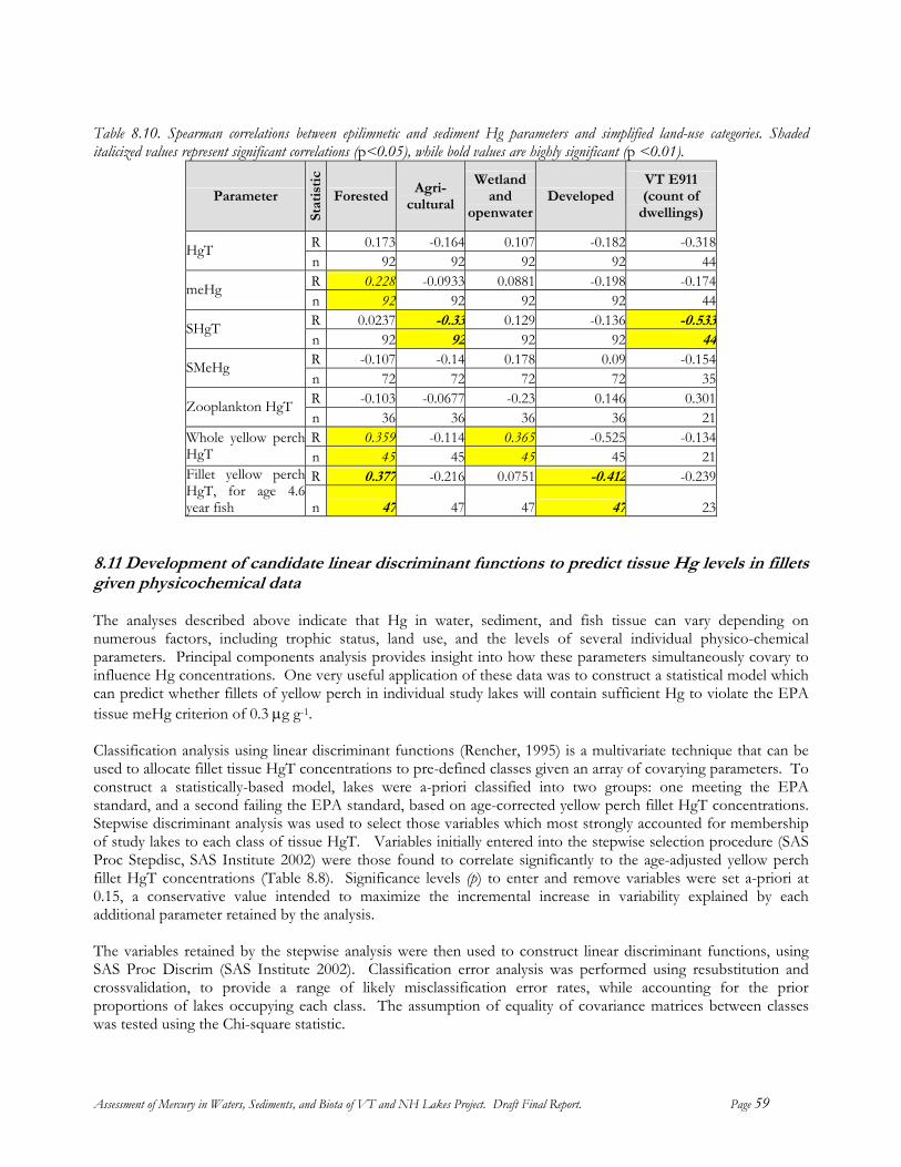
Table 8.10. Spearman correlations between epilimnetic and sediment Hg parameters and simplified land-use categories. Shaded italicized values represent significant correlations (p<0.05), while bold values are highly significant (p <0.01).
Parameter
Stat
isti
c
ForestedAgri-
cultural
Wetland and
openwaterDeveloped
VT E911 (count of
dwellings)
R 0.173 -0.164 0.107 -0.182 -0.318HgT n 92 92 92 92 44R 0.228 -0.0933 0.0881 -0.198 -0.174meHg n 92 92 92 92 44R 0.0237 -0.33 0.129 -0.136 -0.533SHgT n 92 92 92 92 44R -0.107 -0.14 0.178 0.09 -0.154SMeHg n 72 72 72 72 35R -0.103 -0.0677 -0.23 0.146 0.301Zooplankton HgT n 36 36 36 36 21R 0.359 -0.114 0.365 -0.525 -0.134Whole yellow perch
HgT n 45 45 45 45 21R 0.377 -0.216 0.0751 -0.412 -0.239Fillet yellow perch
HgT, for age 4.6 year fish n 47 47 47 47 23
8.11 Development of candidate linear discriminant functions to predict tissue Hg levels in fillets given phys cochemical data i The analyses described above indicate that Hg in water, sediment, and fish tissue can vary depending on numerous factors, including trophic status, land use, and the levels of several individual physico-chemical parameters. Principal components analysis provides insight into how these parameters simultaneously covary to influence Hg concentrations. One very useful application of these data was to construct a statistical model which can predict whether fillets of yellow perch in individual study lakes will contain sufficient Hg to violate the EPA tissue meHg criterion of 0.3 µg g-1. Classification analysis using linear discriminant functions (Rencher, 1995) is a multivariate technique that can be used to allocate fillet tissue HgT concentrations to pre-defined classes given an array of covarying parameters. To construct a statistically-based model, lakes were a-priori classified into two groups: one meeting the EPA standard, and a second failing the EPA standard, based on age-corrected yellow perch fillet HgT concentrations. Stepwise discriminant analysis was used to select those variables which most strongly accounted for membership of study lakes to each class of tissue HgT. Variables initially entered into the stepwise selection procedure (SAS Proc Stepdisc, SAS Institute 2002) were those found to correlate significantly to the age-adjusted yellow perch fillet HgT concentrations (Table 8.8). Significance levels (p) to enter and remove variables were set a-priori at 0.15, a conservative value intended to maximize the incremental increase in variability explained by each additional parameter retained by the analysis. The variables retained by the stepwise analysis were then used to construct linear discriminant functions, using SAS Proc Discrim (SAS Institute 2002). Classification error analysis was performed using resubstitution and crossvalidation, to provide a range of likely misclassification error rates, while accounting for the prior proportions of lakes occupying each class. The assumption of equality of covariance matrices between classes was tested using the Chi-square statistic.
Assessment of Mercury in Waters, Sediments, and Biota of VT and NH Lakes Project. Draft Final Report. Page 59

The stepwise linear discriminant analysis yielded a combination of five covarying parameters (ANC, DOC, pH, conductivity, and flushing rate) that maximized the generalized distance between lakes meeting and failing the USEPA criterion (Wilks’ Λ = 0.32, p<0.0001). The linear discriminant functions necessary to model a lake’s likelihood that muscle tissues of average age 4.6-year yellow perch will meet or violate the USEPA criterion are shown by Equations 1 and 2. Lakes can be attributed to a class by solving each equation using appropriately transformed, lake-specific values. The equation that yields the largest value indicates the class to which the lake would belong, with greater differences between the two solutions indicating a higher confidence in the classification.
DF1 = -1,580 – 82.92(lnANC) + 45.35(lnDOC) + 1,658(ln_pH) - 18.99(lnCond) – 35.09(invrtFlush) Eq. 1 DF2 = -1,494 – 81.94(lnANC) + 48.49(lnDOC) + 1,610(ln_pH) – 18.65(lnCond) – 33.02(invrtFlush) Eq. 2 Where:
DF1 = function to identify lakes with fish tissue HgT concentrations meeting the criterion DF2 = function to identify lakes with fish tissue HgT concentrations failing the criterion lnANC = ln (1+acid neutralizing capacity, in mg l-1, measured from the epilimnion)
lnDOC = ln (1+dissolved organic carbon, in mg l-1, measured from the epilimnion) ln_pH = ln (1+pH, in standard units, average of total water column) lnCond = ln (1+conductivity, in us cm3, average of total water column) invrtFlush = (Flushing rate, in # yr-1)-2
If DF1>DF2, HgT concentrations in tissues of yellow perch are likely to meet the EPA standard. If DF2<DF1, HgT concentrations in tissues of yellow perch are likely to exceed the EPA standard.
---------------------Examples---------------- Log-ANC log-DOC log-pH log-Cond. InvRtFlush DF1 DF2 Class Notch Pond 2.164 2.478 1.948 3.231 0.434 1505.6 1510.1 Fails Paran Lake 5.281 1.404 2.189 5.996 0.168 1554.9 1547.9 Meets
The overall classification error rate was 11.9% and 14.3% based on the resubstitution and crossvalidation methods, respectively. This means that, for Vermont and New Hampshire lakes of greater than 20 acres, we can be confident in using the discriminant functions to predict whether a lake will violate the USEPA tissue Hg criterion, with approximately a 13% chance of misclassifying an individual lake. These models were applied to in a descriptive capacity to classify the remaining 45 REMAP study lakes which did not contain yellow perch, and also to characterize the generalized level of criterion compliance across the entire REMAP dataset. For the lakes without yellow perch, the model indicated that 46.6% (+/- 13.1%) of these lakes would have average age-4.6 year yellow perch fillet concentrations of ≥0.3 µg g-1. Broken down by state, 28.6% of Vermont lakes would show violations of the USEPA criterion, while 62.5% of New Hampshire lakes would be in violation of the criterion. Across the pooled REMAP study lake set (e.g., those lakes with and without yellow perch), the model indicates that 40.2% of lakes may be in violation of the criterion (54% in NH, 25% in VT). The greatest utility of these linear discriminant models is as a screening tool to identify lakes where tissue HgT concentrations are likely to be elevated. Lakes identified as having conditions that support bioaccumulation could be prioritized for sampling to determine actual concentrations, assess model performance, and refine state tissue consumption advisories. A limited test of the statistical model performance can be achieved by applying these models to a separate, independently derived set of lakes with the appropriate parameters and yellow perch tissue data. The Maine REMAP dataset (MEDEP, 1995) provides one such opportunity. In conjunction with the Maine REMAP project, tissues of at least one middle and one upper trophic-level fish species were composited from between two and five fish per lake, across up to 125 lakes over the period 1993-1994. From these 125 lakes, ancillary data
Assessment of Mercury in Waters, Sediments, and Biota of VT and NH Lakes Project. Draft Final Report. Page 60
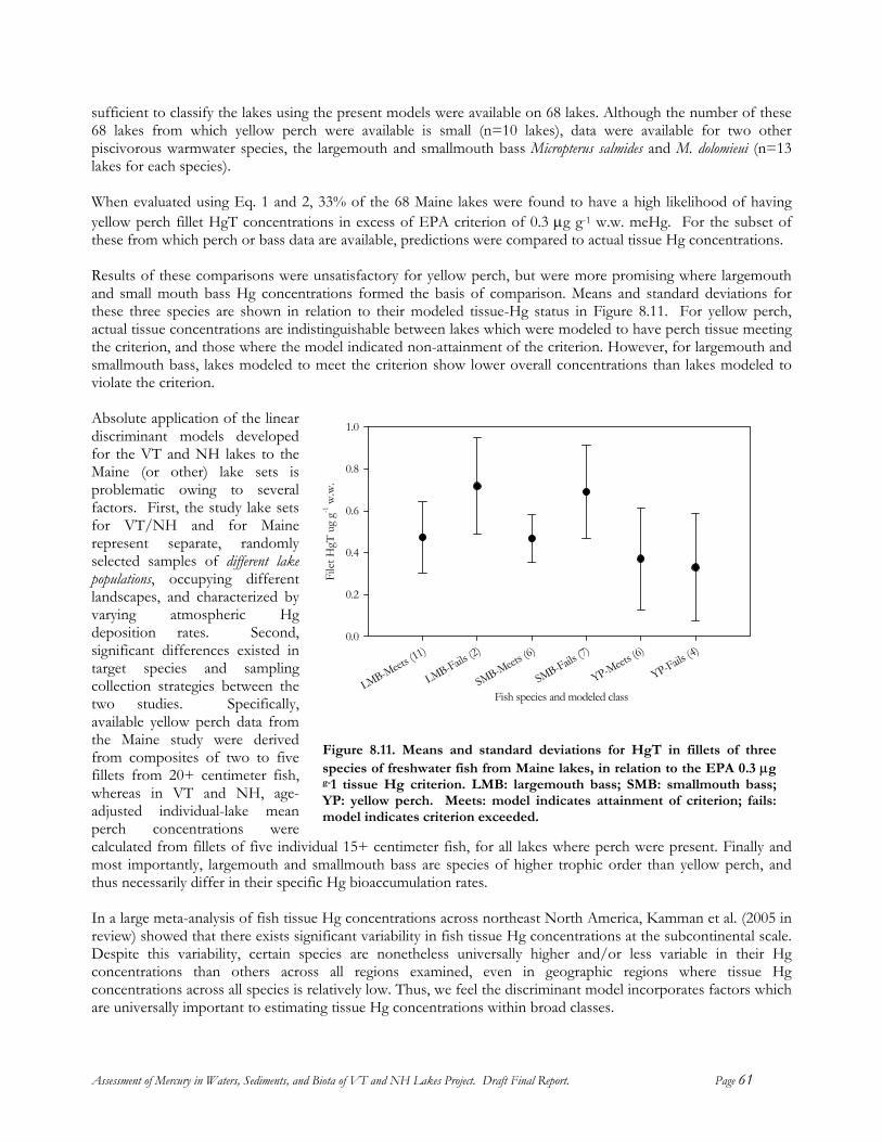
sufficient to classify the lakes using the present models were available on 68 lakes. Although the number of these 68 lakes from which yellow perch were available is small (n=10 lakes), data were available for two other piscivorous warmwater species, the largemouth and smallmouth bass Micropterus salmides and M. dolomieui (n=13 lakes for each species). When evaluated using Eq. 1 and 2, 33% of the 68 Maine lakes were found to have a high likelihood of having yellow perch fillet HgT concentrations in excess of EPA criterion of 0.3 µg g-1 w.w. meHg. For the subset of these from which perch or bass data are available, predictions were compared to actual tissue Hg concentrations. Results of these comparisons were unsatisfactory for yellow perch, but were more promising where largemouth and small mouth bass Hg concentrations formed the basis of comparison. Means and standard deviations for these three species are shown in relation to their modeled tissue-Hg status in Figure 8.11. For yellow perch, actual tissue concentrations are indistinguishable between lakes which were modeled to have perch tissue meeting the criterion, and those where the model indicated non-attainment of the criterion. However, for largemouth and smallmouth bass, lakes modeled to meet the criterion show lower overall concentrations than lakes modeled to violate the criterion. Absolute application of the linear discriminant models developed for the VT and NH lakes to the Maine (or other) lake sets is problematic owing to several factors. First, the study lake sets for VT/NH and for Maine represent separate, randomly selected samples of different lake populations, occupying different landscapes, and characterized by varying atmospheric Hg deposition rates. Second, significant differences existed in target species and sampling collection strategies between the two studies. Specifically, available yellow perch data from the Maine study were derived from composites of two to five fillets from 20+ centimeter fish, whereas in VT and NH, age-adjusted individual-lake mean perch concentrations were calculated from fillets of five individual 15+ centimeter fish, for all lakes where perch were present. Finally and most importantly, largemouth and smallmouth bass are species of higher trophic order than yellow perch, and thus necessarily differ in their specific Hg bioaccumulation rates.
Fish species and modeled classLMB-Meets
(11)
LMB-Fails (2)
SMB-Meets (6)
SMB-Fails (7)
YP-Meets (6)
YP-Fails (4)
File
t HgT
ug
g-1 w
.w.
0.0
0.2
0.4
0.6
0.8
1.0
Figure 8.11. Means and standard deviations for HgT in fillets of threespecies of freshwater fish from Maine lakes, in relation to the EPA 0.3 µgg-1 tissue Hg criterion. LMB: largemouth bass; SMB: smallmouth bass;YP: yellow perch. Meets: model indicates attainment of criterion; fails:model indicates criterion exceeded.
In a large meta-analysis of fish tissue Hg concentrations across northeast North America, Kamman et al. (2005 in review) showed that there exists significant variability in fish tissue Hg concentrations at the subcontinental scale. Despite this variability, certain species are nonetheless universally higher and/or less variable in their Hg concentrations than others across all regions examined, even in geographic regions where tissue Hg concentrations across all species is relatively low. Thus, we feel the discriminant model incorporates factors which are universally important to estimating tissue Hg concentrations within broad classes.
Assessment of Mercury in Waters, Sediments, and Biota of VT and NH Lakes Project. Draft Final Report. Page 61

8.12 Summary of statistical analyses The analyses presented perviously permit the following summary findings: Yellow perch fillet mean HgT concentrations for the present study lakes are most accurately estimated using age as a covariate. The overall average yellow perch fillet HgT concentration, adjusted to an age 4.6 year fish, was 0.225 µg g-1 w.w. Reviewed geographically, the raw data for Hg in water, sediment, and biota indicate that New Hampshire lakes have elevated epilimnetic meHg, hypolimnetic HgT and meHg. Concentrations of hypolimnetic meHg are highest in southern NH. There is a ‘hotspot’ in yellow perch fillet HgT (age-adjusted means) in southwestern NH. The same hotspot is reflected in sediment meHg concentrations, and may reflect a localized Hg source. Evaluation of the stratification imposed upon the random lake selection indicated that no variation in any Hg parameters can be attributed to strata, at a 95% or greater probability level. The stratification was therefore not included in subsequent statistical analyses, although individual lake weighting factors were included in subsequent analyses. Cumulative frequency diagrams based on weighted individual lake mean observations show the likely distribution of Hg in water, sediment, and biota across the region, as well as by state. Based on these diagrams, approximately 25% of lakes across the region possess yellow perch that violate the EPA criterion of 0.3 µg g-1 w.w. meHg in fish tissue. Significant differences between hypolimnetic HgT and meHg, prey and fillet tissue HgT, and zooplankton HgT are apparent between the states, with New Hampshire displaying generally higher overall values. Comparisons are available from the Maine REMAP project, which indicate that while sediment HgT concentrations in Maine are lower than in the Vermont-New Hampshire region, yellow perch tissue concentrations are generally consistent with those of New Hampshire lakes. A formal evaluation of interannual variability indicated that only one parameter – epilimnetic HgT concentrations, varied significantly between years. This variability appears to relate to seasonal rainfall, in that the average HgT concentration across the region was elevated in 1998, coincident with a very wet summer. Year 2000 resamplings of several lakes produced results that were largely unchanged from those in 1998. Observed differences in HgT between year 1998 and 2000 measurements also are related to differences in rainfall. A formal statistical evaluation of the role of trophic status on Hg in waters, sediments, and biota indicated that: 1) epilimnetic HgT and meHg concentrations were elevated in both eutrophic and dystrophic lakes; 2) yellow perch fillet HgT are greatest in dystrophic lakes, and lowest in eutrophic lakes; and, 3) in general, dystrophic lakes can be expected to have HgT fillet concentrations that are 0.218 µg g-1 w.w. greater than in all other lake types. These findings support the hypothesis that Hg is biodiluted in lakes with significant algal production. Mean log-bioconcentration factors ranged from a low of 4.37 for concentration from hypolimnetic HgT to yellow perch fillets, to a high of 6.94 from epilimnetic meHg to loon blood. The bioconcentration factors calculated from our data were consistent with those published elsewhere in the literature. Numerous water chemistry parameters showed significant (p<0.05) correlations to a variety of Hg measurements, in both water and sediment. Data reduction techniques such as principal components analysis were useful to reduce the variability in the dataset, and revealed how covariance among parameters influenced Hg in the study lakes. Such an analysis showed that while HgT and meHg concentrations wre higher both in more acidic lakes and more eutrophic lakes, tissue HgT concentrations only became enhanced in lakes of higher overall acidity. Sediment HgT increased with increasing lake acidity, and decreased where productivity was greatest. This was either the result of bloom dilution and subsequent accumulation to the broad trophic webs characteristic of
Assessment of Mercury in Waters, Sediments, and Biota of VT and NH Lakes Project. Draft Final Report. Page 62
eutrophic lakes, or related to the reduced ability of algal-derived DOC to bind Hg relative to the higher molecular-weight allocthonous DOC characteristic of acidic lake watersheds. Land use characteristics also influence Hg in the present study lakes. As is characteristic of numerous studies, meHg and tissue Hg is elevated in lakes with larger forested and wetland areas. Age-adjusted perch fillet mean HgT is reduced in developed watersheds. Sediment HgT decreases with increasing agricultural area and increased watershed building count. A statistical model was developed permitting to predict if an individual lake would attain or violate the 0.3 µg g-1 w.w. fish tissue meHg criterion, with a 13% likelihood of misclassifying that lake. Application of this model to lakes across the Vermont-New Hampshire region indicated that 40.2% of lakes should have fish sufficiently elevated in HgT to violate the criterion (54% in NH, 25% in VT). Evaluation of model performance using the independently derived Maine REMAP dataset produced mixed results, which were poor when performance was evaluated using yellow perch data, but better when smallmouth and largemouth bass were used. Overall , the statistical models captured those factors which our study indicates are important in estimating whether lakes will have fish tissues in excess of the EPA criterion. Lacking a more detailed, mechanistic model, the statistical model can be used to select lakes outside of the REMAP study set for future sampling, both to verify model performance, and to refine fish tissue advisories.
Assessment of Mercury in Waters, Sediments, and Biota of VT and NH Lakes Project. Draft Final Report. Page 63

9.0 Estimation and mapping of atmospheric Hg deposition 9.1 Summary This section describes the methods used by Ecosystems Research Group, Ltd. to develop estimates of wet and dry mercury deposition to the Vermont and New Hampshire REMAP Lakes Study Area. Estimates were derived at a 30-meter scale ground resolution, allowing the representation at this scale of the effects of geographic location, land cover, forest type, topography, and climate on Hg deposition to the REMAP lake-watersheds. Existing data for total Hg concentrations in precipitation, suspended aerosol particles, and on Hg-vapor from two monitoring networks (MDN and NESCAUM-REMAP) were assimilated and used to interpolate regional concentration fields for seasonal average Hg concentrations in precipitation, suspended particles, and vapor-phase Hg in air. These concentration fields were applied to high-resolution estimates of deposition velocities and precipitation rates calculated by Ecosystems Research Group, Ltd.’s High Resolution Deposition Model (HRDM) to yield localized estimates of Hg transfer to the landscape. Total estimated Hg deposition to the REMAP lake-watersheds was dominated by Hg0 assumed to be assimilated by plant foliage, reactive gaseous Hg deposition, and Hg delivered by precipitation. Particulate-phase and cloud-water Hg deposition were generally unimportant compared to the other pathways. Estimated Hg deposition to the REMAP watersheds ranged from 10.3 µg m-2 y-1 to 32.9 µg m-2 y-1, averaging 22.6 µg m-2 y-1. Estimated total direct deposition to surface waters within the REMAP watersheds ranged from 7.6 µg m-2 y-1 to 16.4 µg m-2 y-1, averaging 9.4 µg m-2 y-1. 9.2 Concentrations of Hg species in the atmosphere There are few direct measurements of mercury in precipitation and the atmosphere relative to the information currently available for estimation of other important air pollutants (S, N, O3) in the study region. However, what information is available is perhaps one of the best regional data sets currently available for atmospheric Hg. The data used to estimate the regional concentration fields for atmospheric Hg species were obtained from the National Atmospheric Deposition Program, Mercury Deposition Network (MDN) and regional studies conducted by NESCAUM.
9.2.1 Hg in precipitation There are 10 locations within or adjacent to the study area where Hg has been measured in precipitation (Table 9.2.1.1) as part of two Hg monitoring networks. Both MDN and NESCAUM network sites measure total Hg in precipitation but use different samplers, protocols and analytical laboratories. The MDN protocol specifies weekly sample collections, while the NESCAUM stations followed the University of Michigan Air Quality Laboratory (UMAQL) protocol which specifies event collections (Burke et al. 1995). Alter (2000) identified a 9 to 22% weekly bias (UMAQL higher) in Hg concentration between collocated samplers using the different samplers, protocols and analytical laboratories for weeks with single and multiple events, respectively. Subsequent collocation trials involving the two differing samplers and protocols but the same (MDN) analytical laboratory found smaller bias (Ann Chalmers and Clyde Sweet, personal communication 2002). Our analysis of the collocated data from the MDN and NESCAUM site at Acadia National Park indicates that on a monthly volume-weighted average basis, the UMAQL protocol determined an average of 38% higher Hg concentrations than the MDN protocol. The relationship between the monthly averages of the two protocols was best modeled by MDN = -1.575634 + 1.3019375*UMAQL -0.0269445*UMAQL2 [Eq. 3] (r2= 0.97, p < 0.0001, n=11, 1 outlier removed) where MDN and UMAQL represent the respective monthly volume-weighted average concentrations of Hg in precipitation in ng l-1 determined by those protocols.
Assessment of Mercury in Waters, Sediments, and Biota of VT and NH Lakes Project. Draft Final Report. Page 64
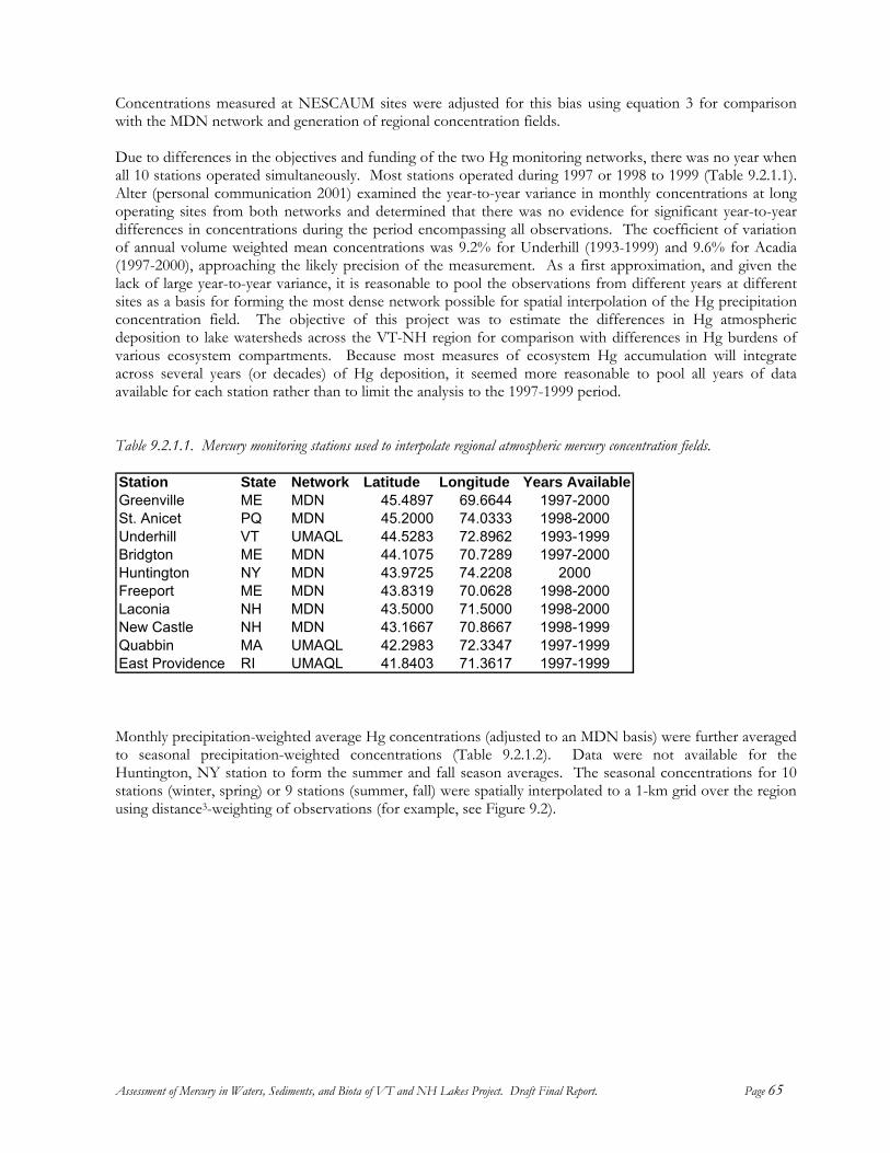
Concentrations measured at NESCAUM sites were adjusted for this bias using equation 3 for comparison with the MDN network and generation of regional concentration fields. Due to differences in the objectives and funding of the two Hg monitoring networks, there was no year when all 10 stations operated simultaneously. Most stations operated during 1997 or 1998 to 1999 (Table 9.2.1.1). Alter (personal communication 2001) examined the year-to-year variance in monthly concentrations at long operating sites from both networks and determined that there was no evidence for significant year-to-year differences in concentrations during the period encompassing all observations. The coefficient of variation of annual volume weighted mean concentrations was 9.2% for Underhill (1993-1999) and 9.6% for Acadia (1997-2000), approaching the likely precision of the measurement. As a first approximation, and given the lack of large year-to-year variance, it is reasonable to pool the observations from different years at different sites as a basis for forming the most dense network possible for spatial interpolation of the Hg precipitation concentration field. The objective of this project was to estimate the differences in Hg atmospheric deposition to lake watersheds across the VT-NH region for comparison with differences in Hg burdens of various ecosystem compartments. Because most measures of ecosystem Hg accumulation will integrate across several years (or decades) of Hg deposition, it seemed more reasonable to pool all years of data available for each station rather than to limit the analysis to the 1997-1999 period. Table 9.2.1.1. Mercury monitoring stations used to interpolate regional atmospheric mercury concentration fields. Station State Network Latitude Longitude Years AvailableGreenville ME MDN 45.4897 69.6644 1997-2000St. Anicet PQ MDN 45.2000 74.0333 1998-2000Underhill VT UMAQL 44.5283 72.8962 1993-1999Bridgton ME MDN 44.1075 70.7289 1997-2000Huntington NY MDN 43.9725 74.2208 2000Freeport ME MDN 43.8319 70.0628 1998-2000Laconia NH MDN 43.5000 71.5000 1998-2000New Castle NH MDN 43.1667 70.8667 1998-1999Quabbin MA UMAQL 42.2983 72.3347 1997-1999East Providence RI UMAQL 41.8403 71.3617 1997-1999 Monthly precipitation-weighted average Hg concentrations (adjusted to an MDN basis) were further averaged to seasonal precipitation-weighted concentrations (Table 9.2.1.2). Data were not available for the Huntington, NY station to form the summer and fall season averages. The seasonal concentrations for 10 stations (winter, spring) or 9 stations (summer, fall) were spatially interpolated to a 1-km grid over the region using distance3-weighting of observations (for example, see Figure 9.2).
Assessment of Mercury in Waters, Sediments, and Biota of VT and NH Lakes Project. Draft Final Report. Page 65
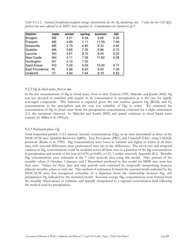
Table 9.2.1.2. Seasonal precipitation-weighted average concentrations for the Hg monitoring sites. Values for the UMAQL protocol sites were adjusted to an MDN basis (equation 3). Concentrations are reported in ng l-1. Station state winter spring summer fallBridgton ME 4.51 6.58 9.85 5.55Freeport ME 4.89 7.11 11.59 7.69Greenville ME 2.79 4.80 9.32 4.82Quabbin MA 5.66 7.35 8.96 6.73Laconia NH 4.81 8.10 8.43 6.20New Castle NH 4.11 7.08 11.82 6.08Huntington NY 5.10 7.20Saint Anicet PQ 5.26 9.09 10.50 8.77East Providence RI 5.68 8.63 8.93 7.09Underhill VT 4.64 7.64 8.19 6.52
9.2.2 Hg in cloud water, frost or dew
e pronounced than site-to-site differences. The site-to-site and temporal variation in Hgp concentrations could be modeled across all three sites as a function of the Hg concentrations in precipitation and month of the year (r2=0.96, p<0.001, n=33, 1 outlier removed, Appendix B.1). Monthly Hgp concentrations were estimated at the 7 other network sites using this model. Nine percent of the monthly values (5 October, 3 January, and 1 December) predicted by this model for MDN sites were less than zero. Values for these sites and time periods were estimated by temporally interpolating between adjacent monthly values at each site. This method of estimation honored the seasonal trends indicated by the NESCAUM sites, but recognized somewhat of a departure from the relationship between Hgp and precipitation Hg indicated by the statistical model. Seasonal average Hgp concentrations were formed from the monthly observations or estimates and spatially interpolated to a regional concentration field following the method used for precipitation.
In the few measurements of Hg in cloud water, frost or dew (Lawson 1999, Malcolm and Keeler 2002) Hg was not elevated or enriched with respect to its concentration in precipitation as is the case for rapidly scavenged compounds. This behavior is expected given the low reactive gaseous Hg (RGM) and Hp concentrations in the atmosphere and the very low solubility of Hg0 in water. We estimated the concentration of Hg in cloud water from the precipitation concentration corrected for a slight enrichment (1.1, the maximum observed by Malcolm and Keeler 2002) and spatial variations in cloud liquid water content (cf. Miller et al. 1993a,b).
9.2.3 Particulate-phase Hg Total suspended particle (<2.5 micron) mercury concentrations (Hgp) in air were determined at three of the NESCAUM sites: Quabbin Reservior (QBN), East Providence (PRV), and Underhill (LKC) using UMAQL protocols (Burke et al. 1995). Hgp concentrations were lower in summer and higher in winter at all three sites, with seasonal differences mor
Assessment of Mercury in Waters, Sediments, and Biota of VT and NH Lakes Project. Draft Final Report. Page 66

Figure 9.2. Estimated Hg concentration (ng l-1) field for summer precipitation. White circles represent the location of mercury monitoring stations (Table 9.2.1.1) used in the interpolation of the regional concentration field. Note: the location of the Huntington, NY site is included in this figure for reference, but there were no summer data available for use in interpolating the concentration field pictured (see text).
Assessment of Mercury in Waters, Sediments, and Biota of VT and NH Lakes Project. Draft Final Report. Page 67
9.2.4 Hg0 vapor Total mercury vapor concentrations (Hgv = Hg0+RGM) in air were determined at three of the NESCAUM sites: Quabbin Reservoir (QBN), East Providence (PRV), and Underhill (LKC) using UMAQL protocols (Burke et al. 1995). In contrast to the Hgp observations, Hgv showed no significant seasonal variation within individual sites. However, individual months were sometimes higher than the mean, indicating the possible importance of significant emission or transport events. Hgv concentrations were significantly different between the sites (ANOVA p<0.0001) with the annual means significantly different between each site (Tukey-Kramer HSD), suggesting a south-to-north or urban-to-rural trend (PRV>QBN>LKC). Analysis of covariance of seasonal mean Hgv with the seasonal average precipitation Hg concentration as the covariate and season as the main effect, revealed the expected seasonal relationship between Hgv and precipitation Hg (r2=0.95, p=0.016, n=12). Hgv was positively correlated with Hg in precipitation, reflecting spatial patterns in atmospheric Hg burdens, while the residuals of this effect were lower in summer and higher in winter reflecting greater oxidation and scavenging rates in summer (Lin and Pekonen 1999). This model formed the basis for estimating Hgv concentrations at the other network sites (Appendix B.2). Seasonal average Hgv concentration observations and estimates were spatially interpolated to a regional concentration field following the method used for precipitation.
9.2.5 Reactive gaseous Hg Reactive gaseous Hg concentrations (RGM = HgCl2 + HgBr2) were not measured by either network. Recent studies suggest that RGM can represent 1-3% of Hgv at continental sites (Lindberg and Stratton, 1998; Landis et al. 2002). Because RGM is highly reactive and rapidly scavenged by moist particles and surfaces, RGM concentrations likely fall off rapidly with distance from their primary sources, incinerators and power plants (Lindberg and Stratton, 1998). Thus, RGM concentrations in the study region are likely to be highly variable and related to point sources. Estimation of the effect of point sources on the spatial distribution of RGM in the atmosphere is beyond the scope of this project. For the purpose of providing bounded estimates of total Hg deposition we estimated RGM deposition for the region assuming RGM represents either 1% or 3% of Hgv. 9.3 Atmosphere-land surface transfers of Hg The exchange of Hg between the atmosphere and ecosystems is bidirectional. Precipitation, dry particle deposition, RGM deposition and Hg0-vapor deposition contribute Hg to landscape burdens. Oxidized forms of Hg in soils, soil waters, surface waters and aquatic sediments are reduced by both biotic and abiotic processes to form Hg0. Because Hg0 is sparingly soluble in water, most of the Hg0 produced in terrestrial and aquatic systems is partitioned into the vapor phase and reemitted to the atmosphere. The primary controls on Hg0 emissions from different landscape elements are just beginning to be well understood. The accumulated landscape burden, bioavailability, and persistence Hg in the environment are all affected by the balance of Hg deposition and reemission. Modeling Hg reemission processes is beyond the scope of this project. The deposition component of atmosphere-surface exchange processes were modeled using Ecosystems Research Group, Ltd.’s High-Resolution Deposition Model (HRDM, Miller 2000). Important data sources for the HRDM are described in Appendix C. We also developed a provisional method to estimate the net Hg0 deposition (net of canopy assimilation and reemission) using foliar Hg accumulation rates, although the mechanisms governing Hg0 exchange processes and foliar sequestration of Hg are currently poorly understood.
9.3.1 Precipitation We estimated the spatial distribution of Hg deposition due to precipitation by multiplying the seasonal average Hg precipitation concentration fields (described above) by the seasonal 30-y normal precipitation fields derived for the HRDM (Miller 2000). Briefly, a regression model was developed to extract the elevation component of the variance in seasonal precipitation rates measured in the NOAA cooperative
Assessment of Mercury in Waters, Sediments, and Biota of VT and NH Lakes Project. Draft Final Report. Page 68
observer network for the Northeastern US (619 stations). The elevation regression model captures local orographic effects on the precipitation rate. The residuals of this model were spatially interpolated to provide local estimates of medium-scale orographic and moisture source effects (Dingman 1981). The regression model is then applied to a high-resolution digital elevation model (DEM) and combined with the residual field to provide a localized estimate of seasonal precipitation rate.
9.3.2 Cloud water deposition The cloud water deposition model of Miller et al. (1993a,b) was parameterized with representative canopy configurations for the major surface types expected to receive cloud water deposition. Multiple sensitivity analyses were conducted with the multi-layer model in order to characterize model response to a large set of possible canopy by meteorological condition interactions. We then statistically apportioned the multi-layer model response to key environmental parameters that can be obtained for each 30-m pixel (wind speed, temperature, LWC, cloud frequency). Cloud frequency is taken to be a function of elevation as observed at Whiteface Mountain, NY (Miller et al. 1993b) but adjusted for regional variation in atmospheric water vapor content using the ratio of sea level precipitation rate at a given location relative to the value at Whiteface Mountain. LWC was estimated from cloud frequency (Miller and Friedland 1999).
9.3.3 Dry deposition of Hgp, RGM, and Hg0
Dry deposition of Hgp, RGM, and Hg0 were estimated using the approach of Lindberg et al. (1992) with some differences and additions described below. Dry deposition velocities for aerosol particles and gasses were estimated using a big leaf model designed for complex terrain and multi-species canopies (Miller et al. 1993a,b). This model includes appropriate physics to simulate deposition to a complex landscape with a wide range of elevations, pressures, temperatures, and receptor surface types. A big-leaf model is preferred over a multi-layer model for this application because of the limited information available to properly characterize the receptor surface at each 30-m pixel. The meteorological data required to drive the dry deposition model (temperature, relative humidity, wind speed, percent of possible solar radiation) were derived from hourly observations at 3 stations within the region of interest, extrapolated on the basis of terrain functions (for example see Miller et al. 1993b) and regional climatology fields (Miller 2000). Total potential solar radiation at a site was calculated taking into account the effects of terrain, and atmospheric optical properties on direct and diffuse solar radiation. The total possible solar radiation was multiplied by the value of percent possible radiation interpolated for a location from the values observed for that hour at the 3 observation stations. The meteorological stations used for this analysis were the Underhill (VT) NOAA site, the Lye Brook Wilderness (VT) CASTNET site, and the Woodstock (NH) CASTNET site. Dry deposition to water surfaces was calculated following the method of Xu et al. (1999). RGM was assumed to behave similarly to nitric acid vapor (Lindberg et al. 1992, Rea et al. 2001) and Hg0 deposition was computed without regard to a compensation point (see below).
9.3.4 Net Hg0 deposition inferred from Hg accumulation in foliage and leaf litter fall rates The Lindberg et al. (1992) model clearly overestimates Hg0 deposition (S.E. Lindberg personal communication 2002) because it does not include a compensation point for Hg (Hanson et al. 1995) as is necessary for modeling other atmospheric species with bi-directional fluxes (e.g. van Hove et al. 2002) and it lacks representation of canopy emission of Hg0 (Lindberg et al. in press, Lindberg and Meyers 2002, Lindberg et al. 1998). Xu et al. (1999) side-stepped modeling a compensation point by separately calculating Hg0 deposition according to Lindberg et al. (1992) and formulating a separate model for canopy emission of Hg0 that is consistent with the very limited pre-1999 understanding of controls on this process. Net Hg0 deposition was taken to be the net of the two model results. Unfortunately several key parameters in Xu et al.’s (1999) canopy emission model – such as the supersaturated concentration of Hg0 dissolved in soil water – remain highly uncertain, are likely quite variable, and are difficult to model with available information. Also,
Assessment of Mercury in Waters, Sediments, and Biota of VT and NH Lakes Project. Draft Final Report. Page 69

recent experimental evidence (Johnson et al. in press, Mae Gustin personal communication 2002) indicates that soil emission of Hg0 is not limited by diffusion through soil as was previously thought (see Johnson and Lindberg 1995, Lindberg et al. 1998) and therefore, supersaturation of soil water with dissolved gaseous Hg0 as assumed by Xu et al. (1999) appears unlikely. Recent, intensive measurements of Hg0 emission from vascular plant canopies suggests that some biological process at the root-soil interface may be responsible for the production of Hg0 (bioreduction) and apparent supersaturation of Hg0 in the xylem of plants exhibiting net Hg0 emission (Lindberg in press, S.E. Lindberg personal communication 2002). Rea et al. (2002) measured the accumulation of Hg in the foliage of deciduous trees over the course of the growing season and found that total accumulation was substantially less than Hg0 deposition estimated following Lindberg et al. (1992). Rea et al. (2001) determined that Hgp and RGM dry deposition are rapidly washed off foliar surfaces, and therefore foliar accumulation of Hg most likely represents Hg0 assimilation. Rea et al. (2002) and Grigal (2002) reach the conclusion that accumulation of Hg in foliage most likely represents a net Hg0 flux from the atmosphere to the canopy. However, given the observations of large Hg emissions from a variety of plant canopies (Lindberg et al. 1998, Lindberg and Meyers 2002, Cobos et al. 2002) and strong indications that the source of Hg0 emitted is from (or involves passage through) the roots of the plants (Lindberg and Meyers 2002, Lindberg et al. in press) it seems equally plausible that foliar accumulation of Hg and its transfer to the soil via litterfall could represent Hg recycling rather than atmospheric deposition. In fact, the rate of Hg accumulation in foliage was highly linear with day of year (DOY), with no significant difference between accumulation rates measured by Rea et al. (2002) in two widely separated forests, in two different years, with significantly different meteorological conditions and Hg0 deposition velocities at each site (Figure 3). Hg retained in plant foliage is presumably sequestered in the vacuole space by phytochelatins that bind Hg2+ (Cobbett 2000). The lack of difference in foliar accumulation rates given the difference in deposition velocities for the two sites studied by Rea et al. (2002) suggests that foliar Hg accumulation might be limited by biological processes mediating sequestration of Hg such as the production of phytochelatins or the oxidation of Hg0 to Hg2+ necessary for Hg to be bound and sequestered by phytochelatins. Such limitations would apply to accumulation of Hg0 with either a soil or atmospheric source. Given the possibility that the annual transfer of Hg from foliage to forest floor via litter fall represents net Hg0 deposition (Rea et al. 2002, Grigal 2002), we developed a method to model the accumulation of Hg in foliage of the study area. Observed Hg contents in foliage at Underhill, VT (Rea et al. 2002) are described well by
Hgfoliage(ng g-1) = DOY * 0.20137 – 26.203 [Eq. 4] (r2= 0.99, p<0.0001, n= 4). Foliar Hg accumulation was also linear with a similar accumulation rate (slope of equation 4) at the Pellston, MI site studied by Rea et al. (2002) (Figure 9.3.4). The zero Hg intercept of equation 4 suggests the onset of accumulation occurred on day 130 (May 10th) at the Underhill site (44.53 N) and 5 days later at the Pellston site (45.57 N), both plausible dates for initial swelling of buds at these locations. The Hg accumulation period constitutes the time between the zero Hg intercept and majority leaf fall, and amounts to 140 to 150 days at these two sites, approximating the length of the growing season. The accumulation period was both shorter and the total Hg accumulation less at the more northerly Pellston site. Thus, as a first approximation, we expect the Hg content of deciduous foliage to be a linear function of the length of the growing season.
Assessment of Mercury in Waters, Sediments, and Biota of VT and NH Lakes Project. Draft Final Report. Page 70
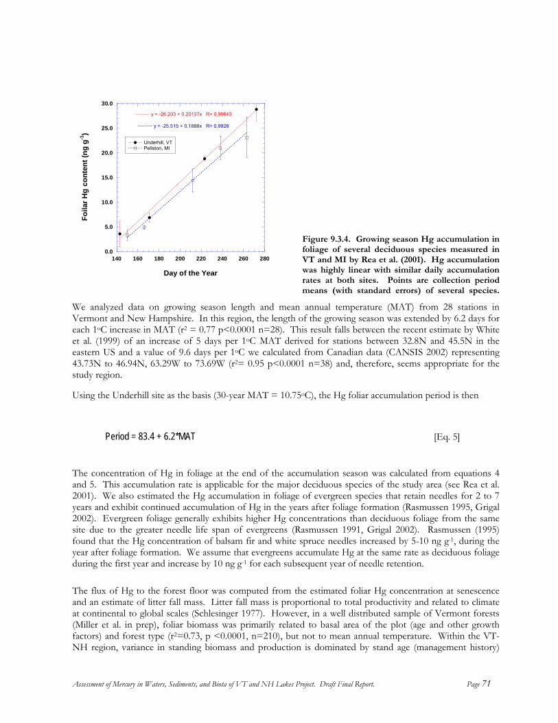
0.0
5.0
10.0
15.0
20.0
25.0
30.0
140 160 180 200 220 240 260 280
Underhill, VTPellston, MI
y = -26.203 + 0.20137x R= 0.99643
y = -25.515 + 0.1888x R= 0.9928
Foila
r Hg
cont
ent (
ng g
-1)
Day of the Year
Figure 9.3.4. Growing season Hg accumulation in foliage of several deciduous species measured in VT and MI by Rea et al. (2001). Hg accumulation was highly linear with similar daily accumulation rates at both sites. Points are collection period means (with standard errors) of several species.
We analyzed data on growing season length and mean annual temperature (MAT) from 28 stations in Vermont and New Hampshire. In this region, the length of the growing season was extended by 6.2 days for each 1oC increase in MAT (r2 = 0.77 p<0.0001 n=28). This result falls between the recent estimate by White et al. (1999) of an increase of 5 days per 1oC MAT derived for stations between 32.8N and 45.5N in the eastern US and a value of 9.6 days per 1oC we calculated from Canadian data (CANSIS 2002) representing 43.73N to 46.94N, 63.29W to 73.69W (r2= 0.95 p<0.0001 n=38) and, therefore, seems appropriate for the study region.
Using the Underhill site as the basis (30-year MAT = 10.75oC), the Hg foliar accumulation period is then
Period = 83.4 + 6.2*MAT [Eq. 5]
The concentration of Hg in foliage at the end of the accumulation season was calculated from equations 4 and 5. This accumulation rate is applicable for the major deciduous species of the study area (see Rea et al. 2001). We also estimated the Hg accumulation in foliage of evergreen species that retain needles for 2 to 7 years and exhibit continued accumulation of Hg in the years after foliage formation (Rasmussen 1995, Grigal 2002). Evergreen foliage generally exhibits higher Hg concentrations than deciduous foliage from the same site due to the greater needle life span of evergreens (Rasmussen 1991, Grigal 2002). Rasmussen (1995) found that the Hg concentration of balsam fir and white spruce needles increased by 5-10 ng g-1, during the year after foliage formation. We assume that evergreens accumulate Hg at the same rate as deciduous foliage during the first year and increase by 10 ng g-1 for each subsequent year of needle retention. The flux of Hg to the forest floor was computed from the estimated foliar Hg concentration at senescence and an estimate of litter fall mass. Litter fall mass is proportional to total productivity and related to climate at continental to global scales (Schlesinger 1977). However, in a well distributed sample of Vermont forests (Miller et al. in prep), foliar biomass was primarily related to basal area of the plot (age and other growth factors) and forest type (r2=0.73, p <0.0001, n=210), but not to mean annual temperature. Within the VT-NH region, variance in standing biomass and production is dominated by stand age (management history)
Assessment of Mercury in Waters, Sediments, and Biota of VT and NH Lakes Project. Draft Final Report. Page 71

rather than climatic factors (Miller et al. in preparation). Because it is currently impossible to estimate forest age at the spatial resolution of the model, we used the mean foliage biomass (adjusted for evergreen needle retention) to estimate litter fall mass by forest type (Table 9.3.4). Table 9.3.4. Characteristics of regional forest types used in the dry deposition and litter fall Hg accumulation models. Leaf biomass estimates are from the forest survey conducted by Miller et al. (in preparation).
Leaf Biomass g litterfall per Leaf Area (m2 m-2)Forest Type t ha-1 +/-se g leaf biomass per g leaf biomass LAI Sources of allometric equationsDeciduous Forest
1 Paper Birch - White Birch 4.39 1.3 1.0000 0.0180 7.90 W2 White Birch - Northern Hardwoods 3.46 0.32 1.0000 0.0180 6.23 W3 Sugar Maple - Northern Hardwoods 3.46 0.32 1.0000 0.0180 6.23 Whi
hittaker et al. 1974hittaker et al. 1974
ttaker et al. 1974
12 Coastal Oak - Coastal Pine 4.67 na 0.8672 0.0075 3.50 Whittaker et al. 19742.61 1.84 0.8672 0.0075 1.96 Whittaker et al. 1974
pruce - Central Hardwoods 2.02 0.65 0.8672 0.0075 1.52 Whittaker et al. 1974
15 Balsam Fir - Red Spruce - Hemlock - White Pine - Northern Hardwoods 3.33 0.33 0.8331 0.0150 5.00 Whittaker et al. 1974
4 Northern Hardwoods 3.66 0.26 1.0000 0.0203 7.43 Whittaker et al. 19745 Central Hardwoods 3.49 0.82 1.0000 0.0096 3.35 Whittaker et al. 19746 Coastal Oaks 3.27 na 1.0000 0.0096 3.14 Whittaker et al. 1974
Evergreen Forest7 Coastal Pines 4.67 na 0.8672 0.0075 3.50 Whittaker et al. 19748 White Pine 2.18 0.65 0.8672 0.0113 2.46 Whittaker et al. 19749 White Pine - Hemlock - Red Spruce 2.39 0.55 0.6123 0.0113 2.70 estimated from properties of classes 8 and 11
10 Hemlock - Red Spruce 3.23 1.3 0.4849 0.0113 3.65 estimated from properties of classes 8 and 1111 Balsam Fir - Red Spruce 6.65 0.33 0.3574 0.0113 7.51 Miller and Friedland 1992
Mixed Forest
13 White Pine - Central Hardwoods14 White Pine - Hemlock - Red S
16 Balsam Fir - Red Spruce - Sugar Maple - Northern Hardwoods 4.66 0.4 0.5953 0.0132 6.13 estimated from properties of classes 15 and 1717 Balsam Fir - Red Spruce - Paper Birch 6.98 0.75 0.3574 0.0113 7.89 Miller and Friedland 1992
9.4 Tabulation of deposition results for the REMAP Lake-Watersheds VTDEC supplied GIS-coverages containing polygons delineating either segments or the full watershed for the NH and VT study lakes. We selected the study watershed polygons based on the study lake centroids. There was an error in the basin delineation of North Pond near Brookfield, VT. This basin was digitized manually from USGS topographic maps. Unique polygon identifiers were assigned to each of the watershed basin segments and a mask was produced to allow extraction of the deposition estimates by watershed or
asin segment. b 9.5
Discussion
The modeled deposition velocities and corresponding fluxes of Hgp, Hgv, and RGM were consistent with values reported by other investigators using the Lindberg Assuming that dry-deposited Hgp and RGM are washsubsequent rains (Rea et al. 2002), the sum of modeapproximate the Hg flux that would be measured in cavariety of forest types and locations, the ratio of throughf(Grigal 2002). The modeled values for this ratio (assumin v scenario) fall between 1.2 and 1.92 (Figure 9.5.1). If the RGM3 scenario (RGM = 3% Hgv) were used, the modeled ratio of throughfall to precipitation Hg flux would be in excess of 3 for mcomparison suggested that the RGM1 scenario is likely to b
et al. (1992) approach to modeling dry deposition. ed off the canopy with 100% efficiency during led precipitation, Hgp and RGM fluxes should nopy throughfall. In field measurements from a
all to precipitation Hg flux ranged from 1 – 3 g the RGM = 1% Hg
ost of the study watersheds (Figure 9.5.2). This e more realistic.
Assessment of Mercury in Waters, Sediments, and Biota of VT and NH Lakes Project. Draft Final Report. Page 72

11.21.41.61.8
22.22.42.62.8
3
100.0%99.5%97.5%90.0%75.0%50.0%25.0%10.0%2.5%0.5%0.0%
maximum
quartilemedianquartile
minimum
1.9200 1.9200 1.8985 1.8040 1.7300 1.6400 1.5300 1.2900 1.2400 1.2000 1.2000
Quantiles
MeanStd DevStd Err Meanupper 95% Meanlower 95% MeanN
1.61039620.16909230.01316381.63638861.5844038
165
Moments
Mean((ppt+Hgp+RGM1)/ppt)Distributions
Figure 9.5.1. Ratio of modeled “throughfall” (see text) to modeled precipitation flux of Hg. The model results are consistent with field studies that indicate the ratio of throughfall to precipitation typically ranges from 1 – 3 (Grigal 2002).
0
4
8
12
16
20
24
100.0%99.5%97.5%90.0%75.0%50.0%25.0%10.0%2.5%0.5%0.0%
maximum
quartilemedianquartile
minimum
8.7400 8.7400 8.4240 7.9940 7.4700 6.5400 5.6100 4.1540 3.0665 1.9800 1.9800
Quantiles
MeanStd DevStd Err Meanupper 95% Meanlower 95% MeanN
6.3324417 1.4330840.11156546.55273156.1121519
165
Moments
Mean(RGM1%(annual))
0
4
8
12
16
20
24
100.0%99.5%97.5%90.0%75.0%50.0%25.0%10.0%2.5%0.5%0.0%
maximum
quartilemedianquartile
minimum
26.220 26.220 25.281 23.992 22.410 19.620 16.830 12.452 9.198 5.950 5.950
Quantiles
MeanStd DevStd Err Meanupper 95% Meanlower 95% MeanN
18.9979194.29876110.334658119.65871318.337125
165
Moments
Mean(RGM3%(annual))Distributions
Figure 9.5.2. Frequency distributions of modeled RGM flux (µg m-2 y-1) assuming that RGM concentrations are either 1% or 3% of observed total gaseous mercury concentrations.
Model estimates of Hg accumulation in foliage and subsequent deposition via litterfall were generally less than
e estimated Hg0 flux (Figure 9.5.3). As discussed above, the modeled Hg0 flux is clearly an overestimate of overestimate Hg0 deposition if some fraction of the Hg Hg0 entrained in the transpiration stream (Lindberg et al.
ththe Hg0 deposition. The litterfall Hg flux may alsofixed in the leaf is derived from dissolved Hg2+ and1998).
Assessment of Mercury in Waters, Sediments, and Biota of VT and NH Lakes Project. Draft Final Report. Page 73
0
4
8
12
16
20
24
28
100.0%99.5%97.5%90.0%75.0%50.0%25.0%10.0%2.5%0.5%0.0%
maximum
quartilemedianquartile
minimum
14.290 14.290 11.520 10.046 9.335 8.530 7.325 5.728 3.917 1.110 1.110
Quantiles
MeanStd DevStd Err Meanupper 95% Meanlower 95% MeanN
8.21968051.80247030.14032218.49675147.9426096
165
Moments
Mean(Hg(litterfall))
0
4
8
12
16
20
24
28
100.0%99.5%97.5%90.0%75.0%50.0%25.0%10.0%2.5%0.5%0.0%
maximum
quartilemedianquartile
minimum
29.870 29.870 28.403 26.300 25.025 22.800 20.490 18.378 15.079 13.220 13.220
Quantiles
MeanStd DevStd Err Meanupper 95% Meanlower 95% MeanN
22.5951733.0865424 0.24028723.06962822.120718
165
Moments
Mean(Hg0(annual))Distributions
Figure 9.5.3. Frequency distributions of modeled Hg fluxes (µg m-2 y-1) via litterfall (may represent net Hg0 deposition) and Hg0 deposition modeled without regard to a compensation point following Lindberg et al. (1992).
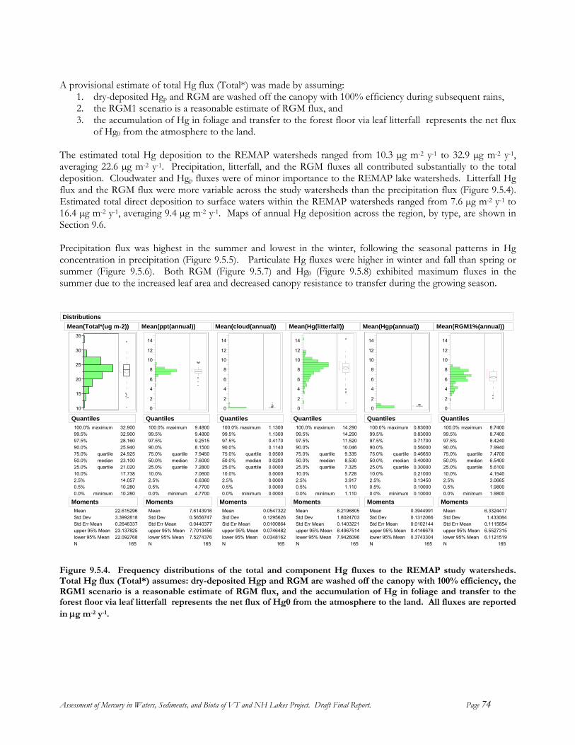
A provisional estimate of total Hg flux (Total*) was made by assuming:
1. 2. 3.
dry-deposited Hgp and RGM are washed off the canopy with 100% efficiency during subsequent rains, the RGM1 scenario is a reasonable estimate of RGM flux, and the accumulation of Hg in foliage and transfer to the forest floor via leaf litterfall represents the net flux of Hg0 from the atmosphere to the land.
The estimated total Hg deposition to the REMAP watersheds ranged from 10.3 µg m-2 y-1 to 32.9 µg m-2 y-1, averaging 22.6 µg m-2 y-1. Precipitation, litterfall, and the RGM fluxes all contributed substantially to the total deposition. Cloudwater and Hgp fluxes were of minor importance to the REMAP lake watersheds. Litterfall Hg flux and the RGM flux were more variable across the study watersheds than the precipitation flux (Figure 9.5.4). Estimated total direct deposition to surface waters within the REMAP watersheds ranged from 7.6 µg m-2 y-1 to 16.4 µg m-2 y-1, averaging 9.4 µg m-2 y-1. Maps of annual Hg deposition across the region, by type, are shown in Section 9.6.
Precipitation flux was highest in the summer and lowest in the winter, following the seasonal patterns in Hg concentration in precipitation (Figure 9.5.5). Particulate Hg fluxes were higher in winter and fall than spring or summer (Figure 9.5.6). Both RGM (Figure 9.5.7) and Hg0 (Figure 9.5.8) exhibited maximum fluxes in the summer due to the increased leaf area and decreased canopy resistance to transfer during the growing season.
10
15
20
25
30
35
100.0%99.5%97.5%90.0%75.0%50.0%25.0%10.0%2.5%0.5%0.0%
maximum
quartilemedianquartile
minimum
32.900 32.900 28.160 25.940 24.925 23.100 21.020 17.738 14.057 10.280 10.280
Quantiles
MeanStd DevStd Err Meanupper 95% Meanlower 95% MeanN
22.6152963.39928180.264633723.13782522.092768
165
Moments
Mean(Total*(ug m-2))
0
2
4
6
8
10
12
14
100.0%99.5%97.5%90.0%75.0%50.0%25.0%10.0%2.5%0.5%0.0%
maximum
quartilemedianquartile
minimum
9.4800 9.4800 9.2515 8.1500 7.9450 7.6000 7.2800 7.0600 6.6360 4.7700 4.7700
Quantiles
MeanStd DevStd Err Meanupper 95% Meanlower 95% MeanN
7.61439160.56567470.04403777.70134567.5274376
165
Moments
Mean(ppt(annual))
0
2
4
6
8
10
12
14
100.0%99.5%97.5%90.0%75.0%50.0%25.0%10.0%2.5%0.5%0.0%
maximum
quartilemedianquartile
minimum
1.1300 1.1300 0.4170 0.1140 0.0500 0.0200 0.0000 0.0000 0.0000 0.0000 0.0000
Quantiles
MeanStd DevStd Err Meanupper 95% Meanlower 95% MeanN
0.05473220.12956260.01008640.07464820.0348162
165
Moments
Mean(cloud(annual))
0
2
4
6
8
10
12
14
100.0%99.5%97.5%90.0%75.0%50.0%25.0%10.0%2.5%0.5%0.0%
maximum
quartilemedianquartile
minimum
14.290 14.290 11.520 10.046 9.335 8.530 7.325 5.728 3.917 1.110 1.110
Quantiles
MeanStd DevStd Err Meanupper 95% Meanlower 95% MeanN
8.21968051.80247030.14032218.49675147.9426096
165
Moments
Mean(Hg(litterfall))
0
2
4
6
8
10
12
14
100.0%99.5%97.5%90.0%75.0%50.0%25.0%10.0%2.5%0.5%0.0%
maximum
quartilemedianquartile
minimum
0.830000.830000.717000.560000.466500.400000.300000.210000.134500.100000.10000
Quantiles
MeanStd DevStd Err Meanupper 95% Meanlower 95% MeanN
0.39449910.13120660.01021440.41466780.3743304
165
Moments
Mean(Hgp(annual))
0
2
4
6
8
10
12
14
100.0%99.5%97.5%90.0%75.0%50.0%25.0%10.0%2.5%0.5%0.0%
maximum
quartilemedianquartile
minimum
8.7400 8.7400 8.4240 7.9940 7.4700 6.5400 5.6100 4.1540 3.0665 1.9800 1.9800
Quantiles
MeanStd DevStd Err Meanupper 95% Meanlower 95% MeanN
6.3324417 1.4330840.11156546.55273156.1121519
165
Moments
Mean(RGM1%(annual))Distributions
Figure 9.5.4. Frequency distributions of the total and component Hg fluxes to the REMAP study watersheds. Total Hg flux (Total*) assumes: dry-deposited Hgp and RGM are washed off the canopy with 100% efficiency, the RGM1 scenario is a reasonable estimate of RGM flux, and the accumulation of Hg in foliage and transfer to the forest floor via leaf litterfall represents the net flux of Hg0 from the atmosphere to the land. All fluxes are reported in µg m-2 y-1.
Assessment of Mercury in Waters, Sediments, and Biota of VT and NH Lakes Project. Draft Final Report. Page 74
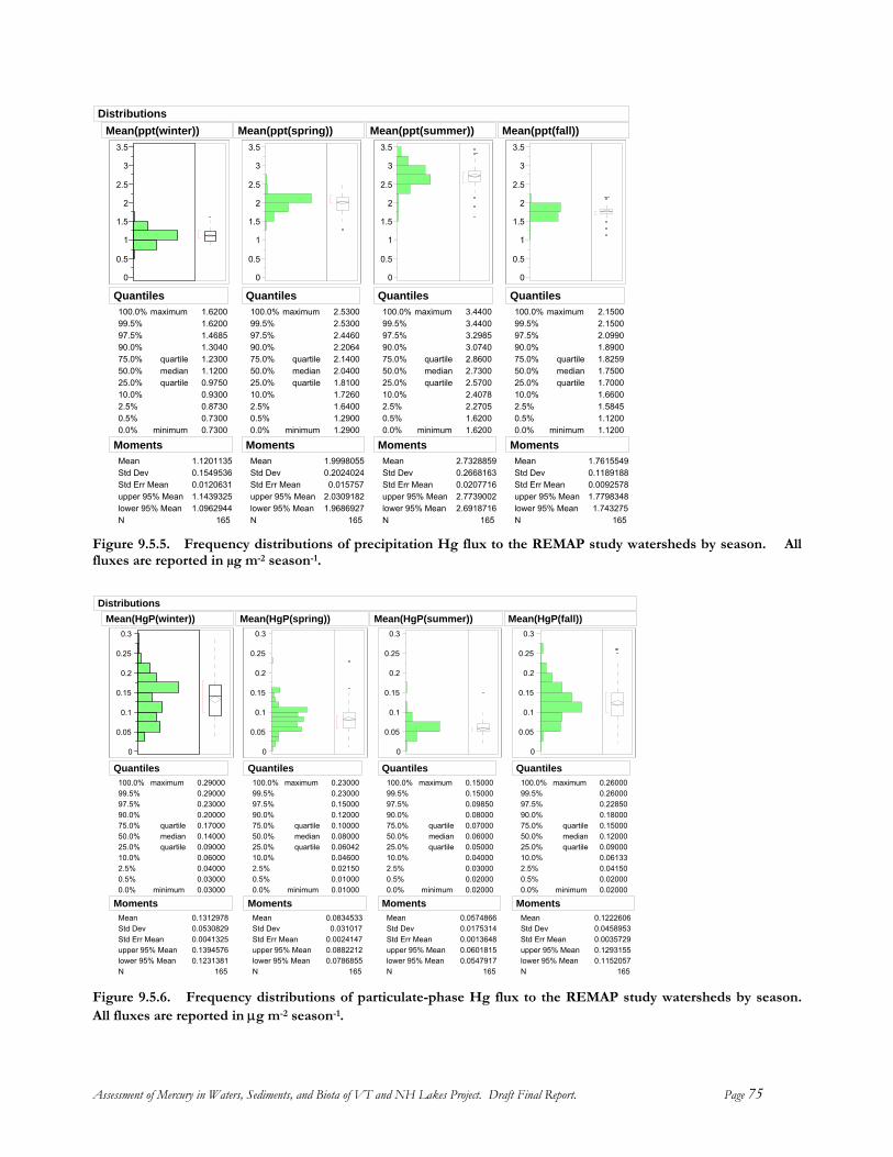
0
0.5
1
1.5
2
2.5
3
3.5
100.0%99.5%97.5%90.0%75.0%50.0%25.0%10.0%2.5%0.5%0.0%
maximum
quartilemedianquartile
minimum
1.6200 1.6200 1.4685 1.3040 1.2300 1.1200 0.9750 0.9300 0.8730 0.7300 0.7300
Quantiles
MeanStd DevStd Err Meanupper 95% Meanlower 95% MeanN
1.12011350.15495360.01206311.14393251.0962944
165
Moments
Mean(ppt(winter))
0
0.5
1
1.5
2
2.5
3
3.5
100.0%99.5%97.5%90.0%75.0%50.0%25.0%10.0%2.5%0.5%0.0%
maximum
quartilemedianquartile
minimum
2.5300 2.5300 2.4460 2.2064 2.1400 2.0400 1.8100 1.7260 1.6400 1.2900 1.2900
Quantiles
MeanStd DevStd Err Meanupper 95% Meanlower 95% MeanN
1.99980550.2024024 0.0157572.03091821.9686927
165
Moments
Mean(ppt(spring))
0
0.5
1
1.5
2
2.5
3
3.5
100.0%99.5%97.5%90.0%75.0%50.0%25.0%10.0%2.5%0.5%0.0%
maximum
quartilemedianquartile
minimum
3.4400 3.4400 3.2985 3.0740 2.8600 2.7300 2.5700 2.4078 2.2705 1.6200 1.6200
Quantiles
MeanStd DevStd Err Meanupper 95% Meanlower 95% MeanN
2.73288590.26681630.02077162.77390022.6918716
165
Moments
Mean(ppt(summer))
0
0.5
1
1.5
2
2.5
3
3.5
100.0%99.5%97.5%90.0%75.0%50.0%25.0%10.0%2.5%0.5%0.0%
maximum
quartilemedianquartile
minimum
2.1500 2.1500 2.0990 1.8900 1.8259 1.7500 1.7000 1.6600 1.5845 1.1200 1.1200
Quantiles
MeanStd DevStd Err Meanupper 95% Meanlower 95% MeanN
1.76155490.11891880.00925781.7798348 1.743275
165
Moments
Mean(ppt(fall))Distributions
Figure 9.5.5. Frequency distributions of precipitation Hg flux to the REMAP study watersheds by season. All fluxes are reported in µg m-2 season-1.
0
0.05
0.1
0.15
0.2
0.25
0.3
100.0%99.5%97.5%
maximum 0.290000.290000.23000
90.0%75.0%50.0%25.0%10.0%2.5%0.5%0.0%
quartilemedianquartile
minimum
0.200000.170000.140000.090000.060000.040000.030000.03000
Quantiles
MeanStd DevStd Err Meanupper 95% Meanlower 95% MeanN
0.13129780.05308290.00413250.13945760.1231381
165
Moments
Mean(HgP(winter))
0
0.05
0.1
0.15
0.2
0.25
0.3
100.0% maximum 0.2300099.5%97.5%90.0%75.0%50.0%25.0%10.0%2.5%0.5%0.0%
quartilemedianquartile
minimum
0.230000.150000.120000.100000.080000.060420.046000.021500.010000.01000
Quantiles
MeanStd DevStd Err Meanupper 95% Meanlower 95% MeanN
0.0834533 0.0310170.00241470.08822120.0786855
165
Moments
Mean(HgP(spring))
0
0.05
0.1
0.15
0.2
0.25
0.3
100.0% maximum 0.1500099.5%97.5%90.0%75.0%50.0%25.0%10.0%2.5%0.5%0.0%
quartilemedianquartile
minimum
0.150000.098500.080000.070000.060000.050000.040000.030000.020000.02000
Quantiles
MeanStd DevStd Err Meanupper 95% Meanlower 95% MeanN
0.05748660.01753140.00136480.06018150.0547917
165
Moments
Mean(HgP(summer))
0
0.05
0.1
0.15
0.2
0.25
0.3
100.0% maximum 0.2600099.5%97.5%90.0%75.0%50.0%25.0%10.0%2.5%0.5%0.0%
quartilemedianquartile
minimum
0.260000.228500.180000.150000.120000.090000.061330.041500.020000.02000
Quantiles
MeanStd DevStd Err Meanupper 95% Meanlower 95% MeanN
0.12226060.04589530.00357290.12931550.1152057
165
Moments
Mean(HgP(fall))Distributions
Figure 9.5.6. Frequency distributions of particulate-phase Hg flux to the REMAP study watersheds by season. All fluxes are reported in µg m-2 season-1.
Assessment of Mercury in Waters, Sediments, and Biota of VT and NH Lakes Project. Draft Final Report. Page 75

0
0.5
1
1.5
2
2.5
3
3.5
100.0%99.5%97.5%90.0%75.0%50.0%25.0%10.0%2.5%0.5%0.0%
maximum
quartilemedianquartile
minimum
2.0800 2.0800 2.0440 1.8940 1.7499 1.5200 1.2700 0.7419 0.5915 0.3900 0.3900
Quantiles
MeanStd DevStd Err Meanupper 95% Meanlower 95% MeanN
1.44696650.39767430.03095891.50809591.3858371
165
Moments
Mean(RGM1(winter))
0
0.5
1
1.5
2
2.5
3
3.5
100.0%99.5%97.5%90.0%75.0%50.0%25.0%10.0%2.5%0.5%0.0%
maximum
quartilemedianquartile
minimum
2.4700 2.4700 2.1785 2.0459 1.8851 1.7000 1.4150 0.7827 0.6115 0.4700 0.4700
Quantiles
MeanStd DevStd Err Meanupper 95% Meanlower 95% MeanN
1.5953003 0.4298960.03346741.66138271.5292178
165
Moments
Mean(RGM1(spring))
0
0.5
1
1.5
2
2.5
3
3.5
100.0%99.5%97.5%90.0%75.0%50.0%25.0%10.0%2.5%0.5%0.0%
maximum
quartilemedianquartile
minimum
3.5100 3.5100 3.2380 2.6680 2.4300 2.0400 1.7232 1.4560 1.1075 0.7200 0.7200
Quantiles
MeanStd DevStd Err Meanupper 95% Meanlower 95% MeanN
2.07725760.51111940.03979062.15582551.9986897
165
Moments
Mean(RGM1(summer))
0
0.5
1
1.5
2
2.5
3
3.5
100.0%99.5%97.5%90.0%75.0%50.0%25.0%10.0%2.5%0.5%0.0%
maximum
quartilemedianquartile
minimum
2.0500 2.0500 1.7700 1.6100 1.4750 1.2300 1.0200 0.6424 0.5015 0.3800 0.3800
Quantiles
MeanStd DevStd Err Meanupper 95% Meanlower 95% MeanN
1.21332520.34142360.02657981.26580791.1608425
165
Moments
Mean(RGM1(fall))Distributions
igure 9.5.7. Frequency distributions of RGM Hg flux (assuming RGM = 1% of measured HgO) to the REMAP udy watersheds by season. All fluxes are reported in µg m-2 season-1.
Fst
02
6
10
14
18
22
100.0%99.5%97.5%90.0%75.0%50.0%25.0%10.0%2.5%0.5%0.0%
maximum
quartilemedianquartile
minimum
4.8400 4.8400 4.3985 4.1580 3.8550 3.3700 2.7700 1.4340 1.1430 0.8100 0.8100
Quantiles
MeanStd DevStd Err Meanupper 95% Meanlower 95% MeanN
3.1668358 0.9270260.07216893.30933583.0243359
165
Moments
Mean(Hg0(winter))
02
6
10
14
18
22
100.0%99.5%97.5%90.0%75.0%50.0%25.0%10.0%2.5%0.5%0.0%
maximum
quartilemedianquartile
minimum
6.9700 6.9700 6.4185 6.0700 5.7350 5.2400 4.5300 3.4860 2.8615 2.6000 2.6000
Quantiles
MeanStd DevStd Err Meanupper 95% Meanlower 95% MeanN
5.02882390.93504050.07279285.17255584.8850919
165
Moments
Mean(Hg0(spring))
02
6
10
14
18
22
100.0%99.5%97.5%90.0%75.0%50.0%25.0%10.0%2.5%0.5%0.0%
maximum
quartilemedianquartile
minimum
22.430 22.430 19.573 14.732 11.830 9.890 8.640 7.862 6.980 6.180 6.180
Quantiles
MeanStd DevStd Err Meanupper 95% Meanlower 95% MeanN
10.7201643.07105960.239081711.19223910.248089
165
Moments
Mean(Hg0(summer))
02
6
10
14
18
22
100.0%99.5%97.5%90.0%75.0%50.0%25.0%10.0%2.5%0.5%0.0%
maximum
quartilemedianquartile
minimum
5.3600 5.3600 5.1455 4.6700 4.2396 3.6400 3.2100 2.6560 2.0890 1.8500 1.8500
Quantiles
MeanStd DevStd Err Meanupper 95% Meanlower 95% MeanN
3.67961110.74914050.05832053.79476693.5644552
165
Moments
Mean(Hg0(fall))Distributions
Figure 9.5.8. Frequency distributions of Hg0 flux to the REMAP study watersheds by season. All fluxes are reported µg m-2 season-1.
Assessment of Mercury in Waters, Sediments, and Biota of VT and NH Lakes Project. Draft Final Report. Page 76
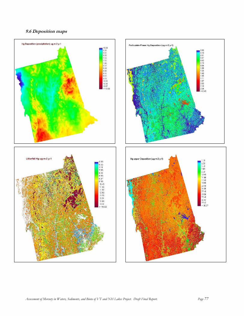
Assessment of Mercury in Waters, Sediments, and Biota of VT and NH Lakes Project. Draft Final Report. Page 77
9.6 Deposition maps
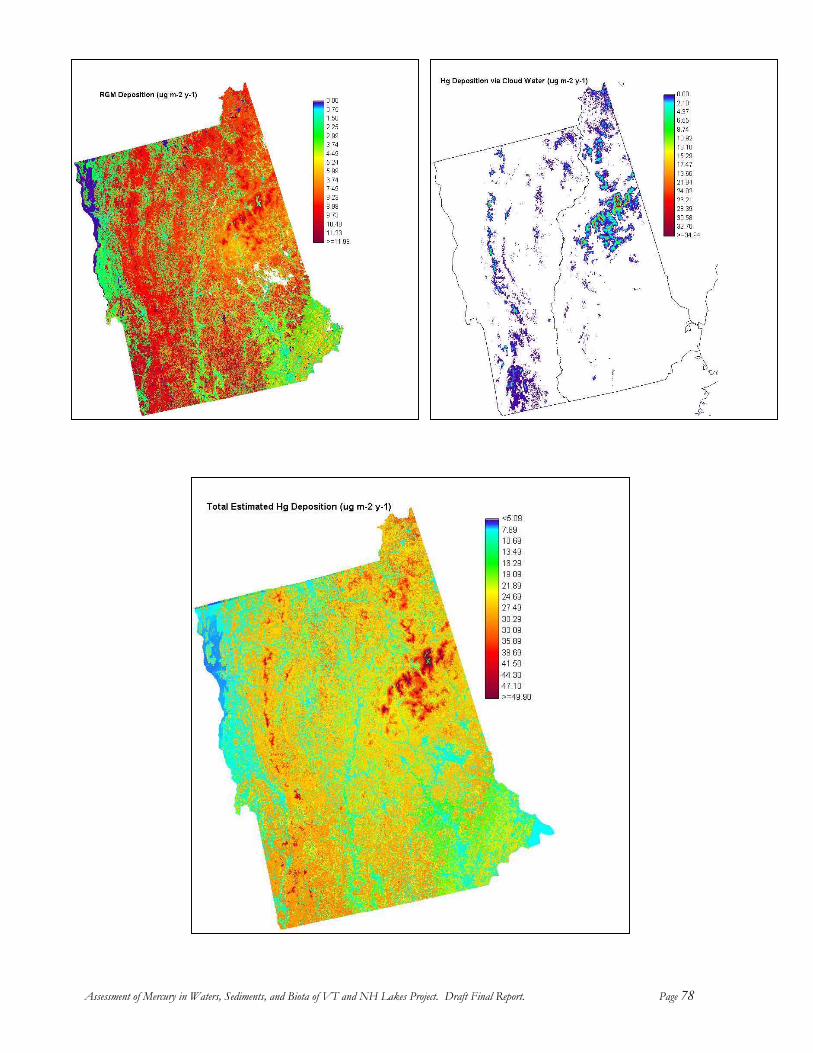
Assessment of Mercury in Waters, Sediments, and Biota of VT and NH Lakes Project. Draft Final Report. Page 78
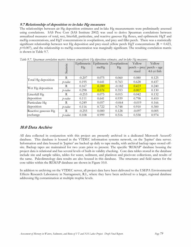
9.7 Relationship of deposition to in-lake Hg measures tionships between air Hg deposition estimates and in-lake Hg measurements wThe rela ere preliminarily assessed
sing correlations. SAS Proc Corr (SAS Institute 2002) was used to derive Spearman correlations between
meHg c statistically significant relationship between wet Hg deposition and prey-sized yellow perch HgT concentrations (R = 0.423,
is shown
able 9.7. Spearman correlation matrix between atmospheric Hg deposition estimates, and in-lake Hg measures.
uannualized measures of total, wet, litterfall, particulate, and reactive gaseous Hg fluxes, and epilimnetic HgT and
oncentrations, and HgT concentrations in zooplankton, and prey and fillet perch. There was a
p=0.007), and the relationship to meHg concentration was marginally significant. The resulting correlation matrix in Table 9.7.
T
Stat
istic
Epilimnetic Hg
Epilimnetic meHg
Zooplankton Hg
Yellow perch – prey
sized
Yellow perch – age 4.6 yr fish
R -0.207 0.075 0.060 0.080 0.125 Total Hg deposition p-value 0.195 0.641 0.763 0.628 0.437 R 0.167 0.280 -0.182 0.423 0.240 Wet Hg deposition p-value 0.298 0.076 0.353 0.007 0.130 R -0.253 0.075 0.015 0.042 0.132 Litterfall Hg
deposition p-value 0.111 0.641 0.939 0.798 0.410 R 0.249 0.057 -0.064 -0.019 0.166 Particulate Hg
deposition p-value 0.116 0.722 0.748 0.910 0.300 R -0.255 0.000 0.128 -0.097 0.005 Reactive gaseous Hg
change p-value 0.1ex 08 0.999 0.516 0.558 0.974 10.0 Data Archive
collected in conjunction with thisAll data project are presently archived in a dedicated Microsoft Access© atabase. This database is housed in the VTDEC information systems network, on the ‘Jupiter’ data server.
site. Bacproject d relational and has several levels of built-in validity checking. Core data tables stored in the database
clude site and sample tables, tables for water, sediment, and plankton and piscivore collections, and results of
core tab
dressing Hg contamination at multiple trophic levels.
dInformation and data housed in ‘Jupiter’ are backed up daily to tape media, with archival backup tapes stored off-
kup tapes are maintained for two years prior to present. The specific ‘REMAP’ database housing the ata is
inthe same. Paleolimnology data results are also housed in this database. The structures and field names for the
les within the REMAP database are shown in Figure 10.0. In addition to archiving on the VTDEC server, all project data have been delivered to the USEPA Environmental Effects Research Laboratory in Narragansett, R.I., where they have been archived to a larger, regional database ad
Assessment of Mercury in Waters, Sediments, and Biota of VT and NH Lakes Project. Draft Final Report. Page 79
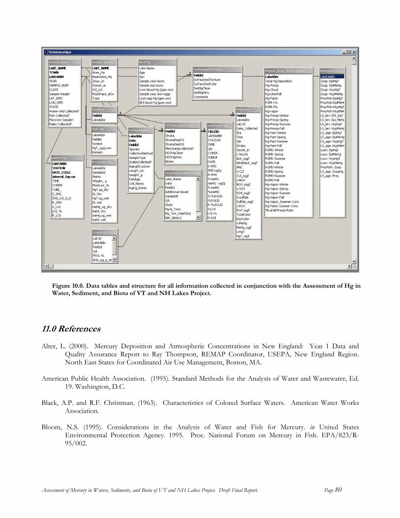
Ass
Am
Bla
11 Al
Blo
Figure 10.0. Data tables and structure for all information collected in conjunction with the Assessment of Hg inWater, Sediment, and Biota of VT and NH Lakes Project.
essment of Mercury in Waters, Sediments, and Biota of VT and NH Lakes Project. Draft Final Report. Page 80
inator, USEPA, New England Region. North East States for Coordinated Air Use Management, Boston, MA.
erican Public Health Association. (1995). Standard Methods for the Analysis of Water and Wastewater, Ed. 19. Washington, D.C.
ck, A
rum on Mercury in Fish. EPA/823/R-95/002.
.0 References
ter, L. (2000). Mercury Deposition and Atmospheric Concentrations in New England: Year 1 Data and Quality Assurance Report to Ray Thompson, REMAP Coord
.P. and R.F. Christman. (1963). Characteristics of Colored Surface Waters. American Water Works Association.
om, N.S. (1995). Considerations in the Analysis of Water and Fish for Mercury. in United States Environmental Protection Agency. 1995. Proc. National Fo

Branfireadwater peatland. Water Resources Research 32: 1785-1794.
1-90.html
un, B.A., A. Heyes, and N. Roulet. (1996). The Hydrology and methylmercury dynamics of a precambrian shield he
Burke, J., M. Hoyer, G. Keeler, and T. Scherbatskoy (1995) Wet deposition of mercury and ambient mercury
concentrations at a site in the Lake Champlain Basin. Water Air and Soil Pollution 80:353-362. Canadian Soil Information System [CANSIS] (2002) Canadian ecosdistrict climate normals 1961-1990.
http://sis.agr.gc.ca/cansis/nsdb/ecostrat/climate_normals_196 Agriculture and Agrifood Canada.
Carter, J ss, S. Beauchamp, G. Brun, and A. d’Entremont. (2001). Mercury concentrations in yellow perch (Perca flavescens) from 24 lakes at Kejimkujik National Park, Nova Scotia. Parks Canada
hen, C.Y., R. Stemberger, B. Klauje, J. Blum, P. Pickhardt, and C. Folt. (2000). Accumulation of heavy metals
Cobbett 25-832.
ingman, S.L. (1981). Elevation: a major influence on the hydrology of New Hampshire and Vermont, USA.
Driscoll son, J. Holsapple. (1994). The Mercury Cycle and Fish in the
Adirondack Lakes. Environ. Sci. Technol. 28:3, 136A-143A.
Electric ric Mercury Deposition. EPRI/TR-106768. Palo Alto, CA.
Evers, Din common loon feathers and blood. Env. Tox. Chem. 17: 173-
183.
Evers, D ercury on piscivorous wildlife as indicated by the Common Loon, 1998-99. Maine Dept. Environ. Protection, Augusta, Maine.
Evers, D hylmercury exposure to piscivorous wildlife in Maine. Maine Dept. Environ. Protection, Augusta, Maine.
Gilmou ions in game fish from Maryland fresh and estuarine waters. Arch. Environ. Contam. Toxicol. 39: 53-59.
Gilmour, L.C., E. Henry, R. Mitchell. (1992). Sulfate Stimulation of Mercury Methylation on Freshwater
anson, P.J., S.E. Lindberg, T.A. Tabberer, J.G. Owens, K.-H. Kim (1995) Foliar exchange of mercury vapor:
. C. Drysdale, N. Burge
Technical Reports in Ecosystem Science # 031. Halifax, Nova Scotia, CA.
Cacross a gradient of lakes. Limnol. Oceanog. 45: 1525-1536.
, C.S. (2000) Phytochelatins and their roles in heavy metal detoxification. Plant Physiology 123:8 Cobos, D.R., J.M. Baker, and E.A. Nater (2002) Conditional sampling for measuring mercury vapor fluxes.
Atmos. Environ. 36:4309-4321.
DHydrological Sciences Bulletin 26:399-413.
, C.T., C. Yan, C. L. Schofield, R. Mun
Power Research Institute, (1996). Protocol for Estimating Historic Atmosphe
.C., J. Kaplan, M. Meyer, P. Reaman, W. Braselton, A. Major, N. Burgess, A. Sheuhammer. (1998).
Geographic trend in mercury measured
. C., C. DeSorbo, and L. Savoy. (2000). Assessing the impacts of methylm
.C.. 2003. Development of a wildlife criterion value to protect against met
r, C. C. and G. Reidel. (2000). A survey of size-specific mercury concentrat
Sediments. Environ. Sci. Technol. 26:11.
Grigal, D.F. (2002) Inputs and outputs of mercury from terrestrial watersheds: a review. Environ. Reviews 10:1-39.
Hevidence for a compensation point. Water, Air , and Soil Pollution 80:373-382.
Assessment of Mercury in Waters, Sediments, and Biota of VT and NH Lakes Project. Draft Final Report. Page 81

Herrin, RT, R.C. Lathrop, P.R. Gorski, A.W. Andren. (1998). Hypolimnetic methylmercury and its uptake by plankton during fall destratification: A key entry point of mercury into lake food chains? Limnol. Oceanog.
Kamman, N.C. and N.M. Burgess. (2005 in review). Mercury in freshwater fish tissues of northeast North
America – a geographic perspective based on fish tissue monitoring databases. Ecotoxicology 14:1-2.
amman, N.C., Lorey, P.M., Driscoll, C.T., Estabrook, R.., Major, A., Pientka, B. and Glassford, E. (2004).
amman, N.C. and D. R. Engstron. (2002). Fluxes of Mercury to Vermont and New Hampshire Lakes Inferred
rement of divalent inorganic reactive gaseous mercury in ambient air. Environ. Sci. Technol. 36: 3000-3009.
awson t. M.S. Thesis. Univ. of Vermont School of Natural Resources, Burlington, VT 05405. 105 p.
Lee, Y., and A. Iverfeldt. (1991). Measurement of Methylmercury and Mercury in Run-off, Lake, and Rain Waters. Wat. Air. Soil Poll. 56: 309-321.
Liang, Lin, C.-J. and S. O. Pehkonen (1999) The chemistry of atmospheric mercury: a review. Atmos. Environ. : 2067-
indber r
indber ercury speciation: concentrations and behavior of
Lindberg, S.E., P. J. Hansen, T.P. Meyers, and K.-H. Kim. (1998). Air/Surface Exchange of Mercury over
indberg
Lindber , W. Dong, and T. Meyers (in press) Transpiration of gaseous elemental mercury through
Lorey, Pof atmospheric mercury deposition. Unpublished PhD
43: 1476-1486. Johnson, D.W. and S.E. Lindberg (1995) The biogeochemical cycling of Hg in forests: alternative methods for
quantifying total deposition and soil emission. Wat. Air Soil Poll. 80:1069-1077.
K
Assessment of mercury in waters, sediments and biota of New Hampshire and Vermont lakes sampled using a geographically randomized design. Environ. Toxicol. Chem. 23: 1172-1186.
Kfrom 210Pb-dates Sediment Cores. Atmos. Environ. 36: 1599-1609
Kuehl, R.O. (2000). Design of experiments: statistical principles of research design and analysis. Duxbury Press. Pacific Grove, CA, USA.
Landis M.S., R.K. Stevens, F. Schaedlich, and E.M. Prestbo (2002) Development and characterization of an
annular denuder methodology for the measu
, S.T. (1999) Cloud Water Chemistry and Mercury Deposition in a High Elevation Spruce-Fir ForesL
. (1996). Chemist, Brooks Rand LTD. Seattle, WA. Personal communication.
L 332079. g, S.E. and T.P. Meyers (2001) Development of an automated micrometeorological method foLmeasuring the emission of mercury vapor from wetland vegetation. Wetlands Ecol. and Manage. 9:333-347.
g, S.E. and W.J. Stratton (1998) Atmospheric mLgaseous mercury in ambient air. Environ. Sci. Technol. 32: 49-57.
Forests – the need for a Reassessment of Continental Biogenic Emissions. Atmos. Environ. 32:895-908.
, S.E., T.P. Meyers, G.E. Taylor, R.R. Turner, and W.H. Schroeder. (1992). Atmosphere-SurfaceLExchange of Mercury in a Forest: Results of Modeling and Gradient Approaches. J. Geophys. Res. 97:2519-2528.
g, S.E.vegetation in a subtropical wetland in Florida. Atmos. Environ.
. M. (2002). The determination of trace levels of mercury in environmental samples in the northeastern U.S. Inferring the past, present, and future
Assessment of Mercury in Waters, Sediments, and Biota of VT and NH Lakes Project. Draft Final Report. Page 82
dissertation. Syracuse University, Department of Civil, Environmental and Chemical Engineering. Syracuse, N.Y.
Maine Department of Environmental Protection. (1995). Fish tissue contamination in Maine lakes, data report.
alcolm, E.G. and G.J. Keeler (2002) Measurements of mercury in dew: atmospheric removal of mercury
Mierle, G. and R. Ingram. (1991). The Role of Humic Substances in the Mobilization of Mercury from
iller, E.K. (2000) Atmospheric Deposition to Complex Landscapes: HRDM – A Strategy for Coupling Deposition Models to a High-Resolution GIS. Proceedings of the National Atmospheric Deposition Program Technical Committee Meeting, October 17-20, 2000, Saratoga Springs, New York.
Miller, E.K. and A.J. Friedland (1999) Local Climate Influences on Precipitation, Cloud Water, and Dry
Deposition to an Adirondack Subalpine Forest: Insights from Observations 1986-1996. J. Environ. Qual. 28:270-277.
Miller, E.K., A. J. Friedland, E.A. Arons, V.A. Mohnen, J.J. Battles, J.A. Panek, J. Kadlecek and A.H. Johnson
(1993b) Atmospheric Deposition to Forests Along an Elevational Gradient at Whiteface Mountain, NY USA. Atmos. Environ., 27A: 2121-2136.
Miller, E.K., J.A. Panek, A.J. Friedland, J. Kadlecek and V.A. Mohnen (1993a) Atmospheric deposition to a high-
elevation forest at Whiteface Mountain, New York, USA. Tellus, 45B, 209-227. Morrison, M.L. (1991). Part 1: Quality Assurance Plan for the Long-term Monitoring Project, in Data User's
Guide for the U.S. EPA Long-term Monitoring Project: Quality Assurance Plan and Data Dictionary. EPA/600/3-91/072. Corvallis, Oregon.
National Weather Service. (2002). Burlington VT Local Climatology. Internet URL
http://www.erh.noaa.gov/btv/html/climo2.shtml
Regional environmental monitoring and assessment program (REMAP). Augusta, Maine, USA.
Mspecies to a wetted surface. Environ. Sci. Technol. 36: 2815-2821.
Mason, R. P. and K. A. Sullivan. (1998). Mercury and Methylmercury Transport through an urbanized watershed. Wat. Res. 32: 321-330.
Watersheds. Wat. Air. Soil Poll. 56: 349-357. M
. Last accessed 9-2002. Oldfield, F. and P. Appleby. (1984). Empirical Testing of 210Pb dating models for lake sediments, in Lake
Sediments and Environmental History. Univ. of Minnesota Press. Minneapolis. Pickhardt, P.C., C.L. Folt, C. Y. Chen, B. Klaue, and J.D. Blum. (2002) Algal blooms reduce the uptake of toxic
methylmercury in freshwater food webs. Proc. Nat. Acad. Sci. 99(7). 4419-4223. Rasmussen, P.E. (1995) Temporal variation of mercury in vegetation. Wat. Air Soil Poll. 80:1039-1042. Rea, A.W., S.E. Lindberg, and G.J. Keeler (2001) Dry deposition and foliar leaching of mercury and selected
trace elements in deciduous forest throughfall. Atmos. Environ. 35:3453-3462. Rea, A.W., S.E. Lindberg, T. Scherbatskoy, and G.J. Keeler (2002) Mercury accumulation in foliage over time in
tow northern mixed hardwood forests. Wat. Air Soil Poll. 133:49-67. Rencher, A.C. (1995). Methods of Multivariate Analysis. J Wiley and Sons. N.Y. New York USA.
Assessment of Mercury in Waters, Sediments, and Biota of VT and NH Lakes Project. Draft Final Report. Page 83
S
and Systematics 8:51-81.
. Mercury Cycling and Transport in the Lake Champlain Basin in Manley, T. O. and P. Manley, eds. Lake Champlain in Transition: From Research Toward Restoration. American Geophysical Union Water Resources Monograph Series, Volume 14, 1999.
SPSS Science Inc. (2000). SigmaStat v. 2.03 users manual. SPSS Science Inc. Chicago, Il. USA. Tejasen, K. (1999). Assessment of Mercury in Lake Waters in Vermont and New Hampshire. Unpublished
masters thesis, Syracuse University, Department of Civil, Environmental and Chemical Engineering. Syracuse, NY, USA
Ullrich, S.M., T.W. Tanton, and S. Abdrashitova. (2001). Mercury in the aquatic environment: a review of factors
affecting methylation. Crit. Rev. Environ. Sci. 31: 241-293. United States Environmental Protection Agency, (2002). EMAP Site Selection protocols. URL:
http://www.epa.gov/wed/pages/EMAPDesign/site_selection.htm
AS Institute Inc. (2002). SAS Version 8.2a. Users Manual. Cary, N.C. USA.
chlesinger, W.H. (1977) Carbon balance in terrestrial detritus. Annual Rev. Ecol.S hanley, J.B., T. Scherbatskoy, A. Donlon, G. Keeler. (1999)S
United States Environmental Protection Agency, (2001). Water Quality Criterion for the Protection of Human
Health. EPA-823-F-01-001. Washington DC United States Environmental Protection Agency, (1998). Ambient Water Quality Criteria Derivation
Methodology -Human Health, Technical Support Document. EPA/822/B-98/005. Washington, D.C. United States Environmental Protection Agency, (1997). Mercury Study Report to Congress. EPA 425-R97-003.
Washington D.C. United States Environmental Protection Agency, (1996)b. Method 1631: Mercury in Water by Oxidation, Purge
and Trap, and Cold Vapor Atomic Fluorescence Spectrometry EPA/821/R 96 012 Washington D.C United States Environmental Protection Agency, (1996)a. Method 1669 Sampling Ambient Water for
Determination of Trace Metals at Water Quality Criteria Levels. EPA/821/R 96/011 Washington D.C. United States Environmental Protection Agency, (1994). Methods for the Analysis of Metals in Water and
Wastewater EPA/600/R-94/111 Washington D.C. United States Environmental Protection Agency, (1979 revised 1983). Chemical Analysis of Water and Wastes.
EPA/600/4-79/020 Washington D.C. United States Geological Survey, (1992). Multi Resolution Land Characteristics. Internet URL
http://edc.usgs.gov/glis/hyper/guide/mrlc. Last accessed 9-2002. Washington D.C. Van Hove, L.W.A, P. Heeres, and M.E. Bossen (2002) The annual variation in stomatal ammonia compensation
point of rye grass (Lolium perenne L.) leaves in an intensively managed grassland. Atmos. Environ. 36:2965-2977.
Vermont Center for Geographic Information. (1996). Land Use and Cover for VT and the Lake Champlain
Basin. Internet URL http://www.vcgi.org/metadata/view_meta.cfm?metafile=landlandcover_lclu.htm. Last accessed 9-2002. Waterbury, VT USA.
Assessment of Mercury in Waters, Sediments, and Biota of VT and NH Lakes Project. Draft Final Report. Page 84
V ent -305(b) Report. ppendix A. Lake Water Quality Assessment. Waterbury, VT. Available online at ermont Department of Environmental Conservation. (1996). 1996 Water Quality Assessm
Ahttp://www.vtwaterquality.org/Planning/LakeAssessment1996.PDF. Vermont Department of Environmental Conservation. (1992 revised 2001) Quality Assurance Plan.
Waterbury, Vermont, USA. . Laboratory
ermont Department of Environmental Conservation. (1998 rev. 2000). Assessment of Hg in Lake-bed Sediments of Vermont and New Hampshire. Quality Assurance Project Plan. Waterbury, VT, USA.
White, M.A., S.W. Running and P.E. Thornton (1999) The impact of growing-season length variability on carbon assimilation and evapotranspiration over 88 years in the eastern US deciduous forest. Int. J. Biometeorology 42: 139-145.
Xu, X., X. Yang, D.R. Miller, J.J. Helble, and R.J. Carley (1999) Formulation of bi-directional atmosphere-surface exchanges of elemental mercury. Atmos. Environ. 33:4345-4355
V
Assessment of Mercury in Waters, Sediments, and Biota of VT and NH Lakes Project. Draft Final Report. Page 85

Appendix A. Historical and present fluxes of mercury to Vermont and New Hampshire lakes inferred from 210Pb dated sediment cores Reprinted from Atmos. Environ. 36: 1599-1609. Copyright 2002.
Assessment of Mercury in Waters, Sediments, and Biota of VT and NH Lakes Project. Draft Final Report. Appendix

Appendix B: Statistical Models of Atmospheric Hg Concentrations
Appendix B.1: Particulate-phase Hg concentration dependence on MDN basis Hg concentration in precipitation and month of the year. Based on observations at Underhill (VT), Quabbin (MA), and East Providence (RI).
05
1015202530354045
Hg(
p)pg
/m3
Actu
al
0 5 10 15 20 25 30 35 40 45Hg(p)pg/m3 Predicted P=0.0007RSq=0.96 RMSE=2.8599
Actual by Predicted Plot
RSquareRSquare AdjRoot Mean Square ErrorMean of ResponseObservations (or Sum Wgts)
0.9602010.8584912.85987813.13805
33
Summary of Fit
ModelErrorC. Total
Source 23 9 32
DF 1775.9197 73.6101
1849.5298
Sum of Squares 77.2139 8.1789
Mean Square 9.4406F Ratio
0.0007Prob > F
Analysis of Variance
Interceptmonth[apr]:(MDN wet Hg conc-7.44624)month[aug]:(MDN wet Hg conc-7.44624)month[dec]:(MDN wet Hg conc-7.44624)month[feb]:(MDN wet Hg conc-7.44624)month[jan]:(MDN wet Hg conc-7.44624)month[jul]:(MDN wet Hg conc-7.44624)month[jun]:(MDN wet Hg conc-7.44624)month[mar]:(MDN wet Hg conc-7.44624)month[may]:(MDN wet Hg conc-7.44624)month[nov]:(MDN wet Hg conc-7.44624)month[oct]:(MDN wet Hg conc-7.44624)month[sep]:(MDN wet Hg conc-7.44624)month[apr]month[aug]month[dec]month[feb]month[jan]month[jul]month[jun]month[mar]month[may]month[nov]month[oct]
Term24.063971-4.2017335.442395718.3304770.925578326.6527943.0426317-2.686522 2.776505 4.97326
8.248615325.8580192.2039207-3.397039-13.8367829.285928-4.74684355.269179-24.03358-16.64159-4.775426 -23.1879
8.104478812.737304
Estimate3.1865852.1750471.962899 2.194891.3594569.2928143.30810112.298571.589077 2.3257
2.24882727.047122.9205465.3312443.7793814.7347614.21631320.222328.03773411.950414.604059 4.947575.83984423.16449
Std Error 7.55 -1.93 2.77 8.35 0.68 2.87 0.92 -0.22 1.75 2.14 3.67 0.96 0.75 -0.64 -3.66 6.19 -1.13 2.73 -2.99 -1.39 -1.04 -4.69 1.39 0.55
t Ratio<.00010.08540.0217<.00010.51310.01850.38170.83200.11450.06120.00520.36400.46980.53990.00520.00020.28940.02310.01520.19720.32670.00110.19860.5958
Prob>|t|
Parameter Estimates
MDN wet Hg conc[month]month
Source 12 11
Nparm 12 11
DF 926.7676 1146.6266
Sum of Squares 9.4427 12.7448
F Ratio 0.0011 0.0003
Prob > F
Effect Tests
-5-4-3-2-101234
Hg(
p)pg
/m3
Res
idua
l
0 5 10 15 20 25 30 35 40 45Hg(p)pg/m3 Predicted
Residual by Predicted Plot
Whole Model
0
10
20
30
40
Hg(
p)pg
/m3
Leve
rage
Res
idua
ls
-5 0 5 10 15 20 25 30 35MDN wet Hg conc[month]Leverage, P=0.0011
Leverage PlotMDN wet Hg conc[month]
05
1015202530354045
Hg(
p)pg
/m3
Leve
rage
Res
idua
ls
0 10 20 30 40 50 60 70 80month Leverage, P=0.0003
Leverage Plot
apraugdecfebjanjuljunmarmaynovoctsep
Level 20.666932 10.227193 53.349899 19.317127 79.333150 0.030387 7.422386 19.288545 0.876071 32.168450 36.801275 9.286237
Least Sq Mean 4.682030 2.226046 3.836191 3.024495 21.875679 8.083379 12.617032 3.640281 4.145956 5.360909 25.134177 4.183184
Std Error 12.2033 14.3667 24.4317 17.5919 16.8600 7.3083 4.6900 13.6200 9.0083 13.9575 12.8500 12.1867
Mean
Least Squares Means Table
monthResponse Hg(p)pg/m3
Assessment of Mercury in Waters, Sediments, and Biota of VT and NH Lakes Project. Draft Final Report. Appendix

Assessment of Mercury in Waters, Sediments, and Biota of VT and NH Lakes Project. Draft Final Report. Appendix
Appendix B.2: Vapor-phase Hg concentration dependence on MDN basis Hg concentration in precipitation and season of the year. Based on observations at Underhill (VT), Quabbin (MA), and East Providence (RI).
1.25
1.5
1.75
2
2.25
Mea
n(va
por H
g co
nc) A
ctua
l
1.00 1.25 1.50 1.75 2.00 2.25Mean(vapor Hg conc) PredictedP=0.0168 RSq=0.95RMSE=0.1276
Actual by Predicted Plot
RSquareRSquare AdjRoot Mean Square ErrorMean of ResponseObservations (or Sum Wgts)
0.9518720.8676490.1276051.785759
12
Summary of Fit
ModelErrorC. Total
Source 7 4 11
DF 1.2881821 0.0651319 1.3533140
Sum of Squares0.1840260.016283
Mean Square 11.3017
F Ratio
0.0168Prob > F
Analysis of Variance
Interceptseason[fall]:(Mean(MDN wet Hg conc)-7.38807)season[spring]:(Mean(MDN wet Hg conc)-7.38807)season[summer]:(Mean(MDN wet Hg conc)-7.38807)season[winter]:(Mean(MDN wet Hg conc)-7.38807)season[fall]season[spring]season[summer]
Term1.60719510.67223340.67081970.73031410.29579310.3581972-0.146945 -0.90059
Estimate0.0809650.1262040.1836190.1559030.0804250.1016650.1233690.186419
Std Error 19.85 5.33 3.65 4.68 3.68 3.52 -1.19 -4.83
t Ratio<.00010.00600.02170.00940.02120.02440.29950.0085
Prob>|t|
Parameter Estimates
Mean(MDN wet Hg conc)[season]season
Source 4 3
Nparm 4 3
DF 1.2568783 0.6816598
Sum of Squares 19.2974 13.9544
F Ratio 0.0070 0.0138
Prob > F
Effect Tests
-0.15
-0.10
-0.05
0.00
0.05
0.10
0.15
Mea
n(va
por H
g co
nc) R
esid
ual
1.00 1.25 1.50 1.75 2.00 2.25Mean(vapor Hg conc) Predicted
Residual by Predicted Plot
Whole Model
1.25
1.50
1.75
2.00
2.25
2.50
Mea
n(va
por H
g co
nc) L
ever
age
Res
idua
ls
1.25 1.50 1.75 2.00 2.25 2.50Mean(MDN wet Hg conc)[season]Leverage, P=0.0070
Leverage PlotMean(MDN wet Hg conc)[season]
1.25
1.50
1.75
2.00
2.25
Mea
n(va
por H
g co
nc) L
ever
age
Res
idua
ls
.5 1.0 1.5 2.0 2.5season Leverage, P=0.0138
Leverage Plot
fallspringsummerwinter
Level 1.9653923 1.4602499 0.7066052 2.2965332
Least Sq Mean0.086953770.131640230.237472990.15362677
Std Error 1.71937 1.85881 1.76414 1.80072
Mean
Least Squares Means Table
seasonResponse Mean(vapor Hg conc)
Assessment of Mercury in Waters, Sediments, and Biota of VT and NH Lakes Project. Draft Final Report. Appendix
Appendix C: Overview of the High Resolution Deposition Model