COMPOUND OPTIONS: A REAL OPTIONS APPLICATION TO …ageconsearch.umn.edu/bitstream/19996/1/sp04br02.pdf · Briggeman, Detre, and Gray Compound Options: A Real Options Application to

Briggeman, Detre, and Gray Compound Options: A Real Options Application to a Food Business 1

COMPOUND OPTIONS: A REAL OPTIONS APPLICATION TO

A FOOD BUSINESS

BRIAN C. BRIGGEMAN, JOSHUA D. DETRE, AND ALLAN W. GRAY1

Real options analysis integrates uncertain outcomes of investment decisions. This framework is used to analyze a new product launch from an agricultural business to a market with multiple uncertainties. Findings indicate a more accurate valuation of the investment when real options and their interactions with the investment are considered. Key words: real options, simulation, uncertainty, strategic management

Introduction

The changing landscape of agriculture has forced those businesses that have a direct linkage

to the agriculture sector to reassess the manner in which they make operational decisions. These

decisions include but are not limited to the following: what is the appropriate price to license a

new technology or a brand, what is the maximum or optimal amount of money that should be

invested in the research and development of a new product, what is the value of being able to

switch input suppliers and/or outsourcers at any time, and how do you value the flexibility of

having the option to defer entry into market.

In today’s agriculture, these operational decisions can no longer be made using the traditional

Net Present Value (NPV) analysis that once dominated corporate strategy. Trigeorgis (1988)

outlines two key areas of value which are not accounted for within a NPV analysis: (1) the

ability of the manager to make operational decisions throughout time or the value of flexibility

1 Brian C. Briggeman and Joshua D. Detre are graduate students in the Department of Agricultural Economics, Purdue University. Allan W. Gray is an associate professor Department of Agricultural Economics, Purdue University. Paper presented during the August 1st - 4th 2004 AAEA meetings in Denver, Colorado. Copyright © 2004 by Brian C. Briggeman, Joshua D. Detre, and Allan W. Gray. All rights reserved. Readers may make verbatim copies of this document for non-commercial purposes by any means, provided that this copyright notice appears on all such copies.


(e.g. defer, abandon, or expand a given project), and (2) the interdependencies of these decisions

on the investment throughout time (e.g. entrance of competition into the market). The

framework needed to address the shortcomings of a traditional NPV analysis must be an

integrated framework that incorporates multiple forms of uncertainty in conjunction with the

flexibility to exercise decisions at any point in time. This examines a simulation approach to real

options, which serves as the integrated framework giving an agribusiness the capabilities to make

these types of decisions. In particular, the decision by Fresh Juice Inc. to either launch a new

product today or wait and see how the market unfolds. In addition to this decision, Fresh Juice

Inc. must also decide whether to bottle the new juice product with a facility built and operated by

Fresh Juice Inc. or to out-source bottling with a co-packer.

Real options are an integrated approach to options theory using financial theory,

economic analysis, management and decision science, statistics, and econometrics. An

important aspect of real options theory is the ability to account for the dynamics and uncertainty

of business decisions. Traditional NPV analyses typically assume a static decision making

process with no recourse in changing those decisions while real options allow the business to

make strategic decisions under uncertainty. Real options give the management flexibility to

assimilate and process these uncertainties over time. One can think of real options as a learning

model that allows the management to make informed and accurate strategic decisions over the

course of time.

Trigeorgis (1988) defines real options as being the owner of a discretionary investment

opportunity who has the right to the investment’s present value of cash flows by making some

initial outlay on or before the termination date of that investment. He later develops a theoretical

framework in which he demonstrates the value of managerial flexibility when strategic decisions


are made throughout time. Bernake (1983) developed a framework to account for the effects of

irreversibility and uncertainty on investments when those investments are cyclical in nature. He

posits that incorporating the flow of information throughout time can create a positive incentive

to undertake the investment; in essence the manager takes a “learning-by-doing” approach to the

investment. Dixit (1989) and McDonald and Siegel (1986) consider a real options approach to

investment under uncertainty wherein they look at optimal trigger values indicating when a firm

should enter or exit the given investment. Copeland and Keenan (1998) employ real options to a

case study which looks at the decision to build or not to build a factory which has a significant

amount of uncertainty surrounding its profits. Luehrman (1998) introduces a NPV metric that

links corporate discounted cash flow (DCF) methods to the classic (Black-Scholes) Model. The

motivation for Luehrman’s NPV metric is to circumvent the complex mathematical calculations

necessary for a real options analysis by allowing managers a way to introduce uncertainty into

their preexisting DCF models. Each of these contributions to the real options literature

highlights the importance of agribusinesses adopting a real options framework or at least the

mentality of real options when making investment decisions.

Fresh Juice Inc., adopted from Gray (2000), is in the process of launching a new GMO

juice into the marketplace. In launching this new product, Fresh Juice Inc. has many questions

about that product or real options theory is applied to disentangle this web of uncertainty. Two

areas of uncertainty are considered given their importance to a new product launch. 1) The time

of entry of the product into the market. A growth or expansion option allows Fresh Juice Inc. to

place a value on first mover advantages within the given market. Conversely, Fresh Juice Inc.

potentially has value in waiting for some of the uncertainties to be revealed which is captured by

the option to defer. 2) The ability of Fresh Juice Inc. to use alternative technologies, which


directly affect the product. An example would be a flexible production contract. The firm can

terminate the production contract and move to a least cost method of production at any time.

Valuation of this is done through the use of a switching option.

Although these options can be valued independently, there exist interdependences

between these options. These interactions create additional option value to the firm and must be

accounted for. The flexibility of altering production processes, i.e. switching option, has a direct

effect upon the valuation of the option to grow or defer. This relationship can be viewed as a

staged investment problem, which revolves around the asset specificity of the capital outlay.

Initial design choice of the production processes allows management to choose outsourcing or

in-house production when dealing with large amounts of uncertainty and asset specificity.

Without this initial design choice, the sequential interdependences among the options are

overlooked and can lead to incorrect investment decisions by the Fresh Juice Inc.

From here we look at the methodology used to analyze the decision faced by Fresh Juice

Inc. Next is a discussion of the data collected from Fresh Juice Inc. followed by the results of

the real options analysis. Finally, the conclusions of the analysis are addressed and their

implications towards further use in the agribusiness literature.

Methodology/Data

Option to Defer

Options are widely used within financial markets so as to allow uncertainty surrounding

the given stock/commodity to unfold over time while maintaining the option to enter the market

at a specified price. It is apparent when financial options should be utilized in a firm’s risk

management strategy however, real options are not as noticeable and can be applied in situations

in which a financial option does not exist. Dixit and Pindyck (1994), state that real options are


applicable in situations where uncertainty, irreversibility, and the owner of the real option can

delay entry. Thus the option to defer can be thought of as a strategic option that gives the owner

or decision maker the ability to hedge their investment decision against any downside risk.

In keeping with the analogy between financial options and real options, the option to

defer can be thought of as a call option. (Mun 2002) presents a slightly adjusted Black-Scholes

model so as to use the model as an option to defer:

(1) ( )

Option to defer S d Xe d

d

S

XT r

T

d d T

tr T

of

f= −

=

+ +

= −

−Φ Φ( ) ( )

ln

1 2

1

2

2 1

12σ

σσ

Where S is the value of the underlying asset and is indexed on time t; Φ is the cumulative

standard normal distribution function; X is the cost of developing the intangible asset; rf is the

risk free rate; σ is the standard deviation or volatility of cash flows throughout the life of the

investment; T is the economic life of the option to defer.

A limitation of modeling the option to defer via the Black-Scholes model is seen in the

underlying assumptions of the Black-Scholes model. The main assumption is that the price

structure of the intangible asset follows a Geometric-Brownian Motion with a constant drift and

volatility parameters. A Markov-Wiener stochastic process is assumed to represent the motion

portion with the following derivation:

(2) dS uSdt SdZ

dZ dt

= +

=

σε

dZ is a Weiner process; u is the drift rate; σ is the volatility measure. Other assumptions of the

Black-Scholes model are an efficient market with no riskless arbitrage opportunities, no


transaction cost, no taxes, and price changes are continuous and instantaneous. All of these

assumptions are subject to scrutiny especially when applied to a real options context.

Figure 1 provides a graphical demonstration on how a final analysis would appear if the

Black-Scholes model were applied to an option to defer. Given the uncertain fluctuations

surrounding an investment, the option to defer brings additional value to the investment as

shown in the Figure 1. The standard DCF approach has more risk, measured as the standard

deviation (σ) of returns, and a lower average percentage return (µ) when compared to the real

options approach. Elimination of downside risk is highlighted here through the real options

approach because the owner of the option to defer would not execute the option if the returns of

the investment were a worst case scenario over time.

By construction of the Black-Scholes model, the option value cannot take on a negative

value. This is an issue that could cause an owner of an option to defer to “over-value” his or her

investment. For example, an industry leader may feel that a given investment has too much

uncertainty surrounding its success. Therefore, an option to defer is calculated and the results

indicate that there is value in waiting to see how the market unfolds. By waiting to proceed with

the investment, the company may have missed out on any first mover advantages and thus are

now following the market if they do decide to go forward with the investment.

Switching Option

As technology or terms of production change, agribusinesses must reassess if their

current production methods are the least cost method. Mun (2002) addresses this issue via a

switching option. This method puts a value on the firm’s ability to change from one technology

to the next throughout time. Calculating this option is as follows:


(3)

−

+Φ−

−

+Φ−

+

+Φ

T

T

SX

S

XST

T

SX

S

ST

T

SX

S

Sσ

σ

σ

σ

σ

σ2)1(

ln(2)1(

ln(2)1(

ln(2

1

2

1

2

1

2

1

2

1

2

2

S2 represents the new technology asset value; S1 is the current technology asset value; X is a

proportional cost relative to S1; all other notation holds from the option to defer discussion.

Hence, the switching option is interpreted as the optimal time to switch is when the new

technology asset value is greater than the current technology asset value plus any associated

costs with switching. It is interesting to note that as the volatility of S2 increases relative to S1,

the value of the switching option increases. That is as the uncertainty of the cash flows

surrounding the new technology increases; value is created for the switching option owner to

have the ability to change technologies over time.

Compound Option

A compound option considers the value of an option being contingent upon other options

that are executed prior to or during the valuation of the current option. Prior decisions affect the

value of the underlying investment and therefore making future options conditional on exercised

past options. Simply adding up the values of all options considered can dramatically overstate

the total value of the investment and result in incorrect strategic decisions being made.

Trigeorgis (1993) models multiple real options and finds that the interactions of real options

depend on the type, separation of when the options occur, and order in which the options occur.

These interactions can have a positive or negative impact upon the valuation of the investment,

i.e. one option may dominate and actually negate the value of another option we examined in the

context of a compound option. Combining different real options gives management the


flexibility to see the economic value that their decisions will have on the investment throughout

time.

Data and Empirical Model

Fresh Juice Inc. (Fresh Juice Inc. is a fictitious name, but the data underlying the case is

true, the name of the company is change to protect the confidentiality of the firm) is a leader in

the finished consumer juice industry and has been producing and distributing competitively

priced high quality fruit juices to leading national grocery chains for a number of years. While

demand for fruit juice has remained steady over the last 10 years, the increase in the number of

competitors continues to place pressure on Fresh Juice Inc.’s leader status. The intense

competition for shelf space and the continuing fragmentation of consumer’s tastes and

preferences has kept competitors battling each other on price, advertising, and packaging just to

maintain their market share. The product development team’s latest product, GMO Juice (this is

an internal name for the product, the actual name for the product has not been finalized), just

may be the ticket to give Fresh Juice Inc. the new competitive advantage they need in an industry

that has not seen an innovative product in fifteen years.

To analyze the decision of introducing the new GMO Juice to the market a spreadsheet

model was developed in Microsoft Excel to incorporate the uncertainty surrounding the decision.

The @Risk add-in for Microsoft Excel is utilized to run Monte Carlo simulations, with 5,000

iterations for each scenario. Therefore, the model calculates the likelihood of profitability and

the NPV of the project over a ten-year period to determine which alternative produces the

highest payoff for the firm under scenario analysis. This approach to valuing an investment

through simulation techniques was employee by Hyde, Stoke, and Engel (2003).


- Market Size

The current fruit juice market is about 10,000,000 cases annually. Management believes

there is a 90% chance the market for GMO Juice is between 2,250,000 and 2,750,000 cases

annually. Initial analysis assumes 2,500,000 cases as the most likely but the aforementioned

interval recognizes the uncertainty in this estimate of market size. To further supplement these

estimates, Fresh Juice Inc. recently launched a product (ENER Juice) which has similar

characteristics, both in type of juice and market acceptance, to the GMO Juice being considered.

Table 1 outlines the historical information of ENER Juice.

How many cases of GMO juice will be demanded in the market place in each year is

estimated by using ENER Juice data. To calculate GMO Juice demand we take what each

historical year’s sales were for ENER Juice as a percent of the estimated total market size of

2,500,000 of ENER Juice. We use percentages to estimate the following regression equation:

(4) 2

21 ttyt ββα ++=

where yt is the percentage of the total market for each historical year’s sales, t is time, α is a

constant, β1 is a slope coefficient on time, and β2 is a slope coefficient on time squared. This

quadratic regression equation fits the data and produces the classic product adoption curve shape.

- Market Share

Market share is certainly a critical variable in determining the profitability of GMO juice.

It is understood that market share is closely related to the actions of your competitors. The

question is how much impact does each competitor have? Table 2 contains Fresh Juice Inc.’s

estimates for both the relative powers of each competitor and the likelihood (by year for the first

5 years) of each competitor entering the market for GMO Juice.


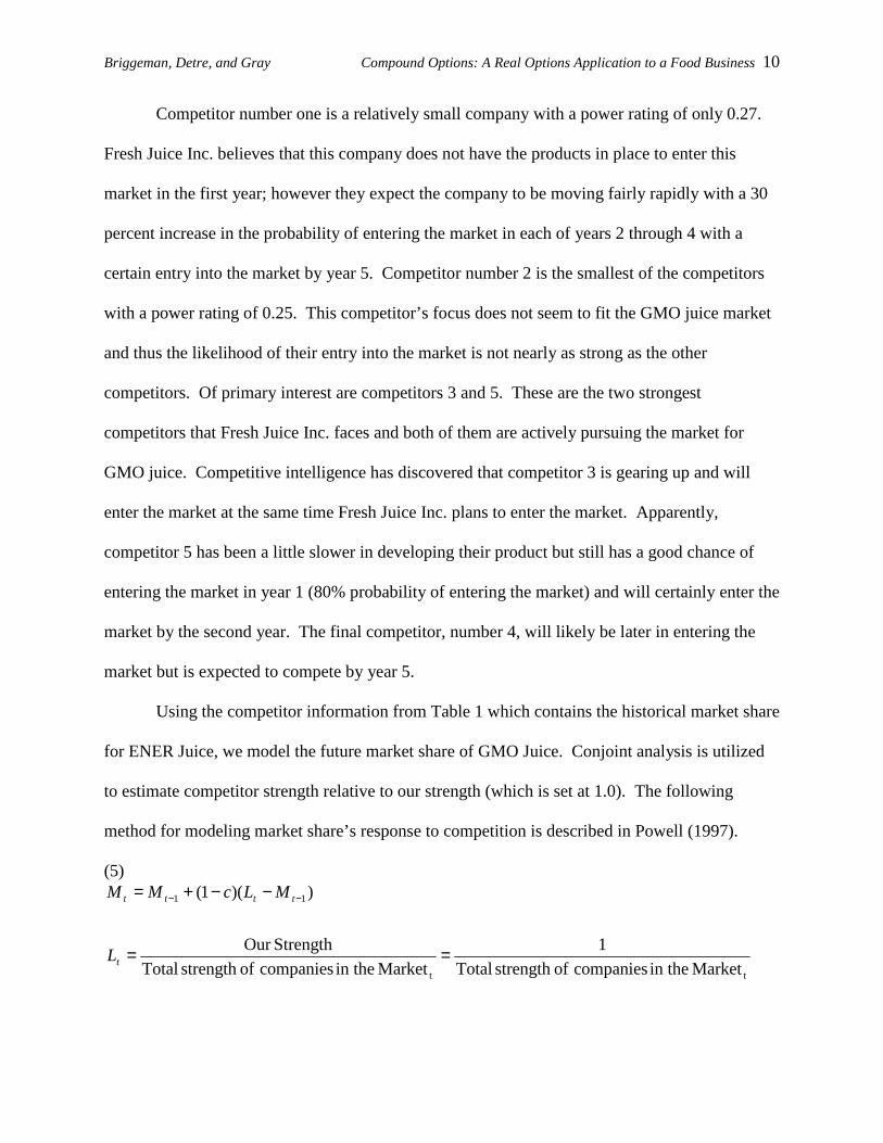
Competitor number one is a relatively small company with a power rating of only 0.27.

Fresh Juice Inc. believes that this company does not have the products in place to enter this

market in the first year; however they expect the company to be moving fairly rapidly with a 30

percent increase in the probability of entering the market in each of years 2 through 4 with a

certain entry into the market by year 5. Competitor number 2 is the smallest of the competitors

with a power rating of 0.25. This competitor’s focus does not seem to fit the GMO juice market

and thus the likelihood of their entry into the market is not nearly as strong as the other

competitors. Of primary interest are competitors 3 and 5. These are the two strongest

competitors that Fresh Juice Inc. faces and both of them are actively pursuing the market for

GMO juice. Competitive intelligence has discovered that competitor 3 is gearing up and will

enter the market at the same time Fresh Juice Inc. plans to enter the market. Apparently,

competitor 5 has been a little slower in developing their product but still has a good chance of

entering the market in year 1 (80% probability of entering the market) and will certainly enter the

market by the second year. The final competitor, number 4, will likely be later in entering the

market but is expected to compete by year 5.

Using the competitor information from Table 1 which contains the historical market share

for ENER Juice, we model the future market share of GMO Juice. Conjoint analysis is utilized

to estimate competitor strength relative to our strength (which is set at 1.0). The following

method for modeling market share’s response to competition is described in Powell (1997).

(5)

tt

11

Market in the companies ofstrength Total

1

Market in the companies ofstrength Total

StrengthOur

))(1(

==

−−+= −−

t

tttt

L

MLcMM


where Mt is our firm’s share of the market in time period t; Lt is our firm’s long-term share of

the market, which is base on our market power relative to the power of all firms in the market

place; (1-c) is a parameter, which measures, in rough terms, the amount of time it takes our firm

to “slide” towards its long-term share given the market share it encountered during the last

period. In order to estimate the aforementioned parameter we estimate the following regression

equation based on ENER Juice information:

(6) ))(1( 11 −− −−=− tttt MLcMM - Prices

To determine the prices to be received for each case of GMO Juice from the retailers, we

use the information on ENER Juice to forecast the price for GMO juice. The following elasticity

equations are used to estimate the price of any product:

(7) 1%,1%

)%%1(

11

1

−=∆−=∆

∆+∆+=

−−

−

t

t

t

t

dstt

S

SS

D

DD

SeDePP

( ) ( )SeDeP

Pds

t

t ∆+∆=

−

−

%ˆ%ˆ11

Pt is the price in period t; es is the elasticity of supply; ed is the elasticity of demand; D is

Demand; S is Supply. Po is given in Table 1, D is calculated in equation 4 and S is based on the

capacity of the industry which is calculated in equations 5 and 6. By using ENER Juice data, the

demand and supply elasticities are estimated through a regression analysis.

- Costs

GMO Juice will require a $150,000 investment in new extractor equipment so as to

extract the juice from the specialized fruit and mix in the necessary ingredients for enhanced


taste and shelf life. In addition, the cost of a new line to bottle and label the juice has been

estimated to cost $1,225,000 for an initial investment cost of $1,375,000. Variable costs per unit

for bottling the GMO Juice ourselves are determined based on the following cost equation:

(9) 2000006.0007.073.2 qqAVCq +−=

Here q is in 1,000 units so to get the variable cost per unit we take the volume sold and divide by

1000 and then use the above equation. For the Co-packing option, variable costs per unit are

$3.05 per bottle constantly. For the “in-house” option, fixed costs are $285,000. For the co-pack

option, there are no fixed costs. Advertising costs have been estimated by the marketing

department and are independent of volume and the type of bottling operation chosen.

Results

The results of the base model for both the bottling and co-packing scenarios yield a

negative expected NPV, of -$540,635 and -$44,823 respectively (Table 1). Analysis also

indicates that the Co-Pack option will have at least a 25% chance of an NPV exceeding

$765,014, while the Bottling option will generate an NPV $292,177 or less 75% of the time. This

provides an indication that the GMO Juice project, with the options currently available to Fresh

Juice Inc. Inc., is a project that is not worth undertaking regardless of the bottling method

chosen.

The next result concerns the introduction of the switching option. The switching option

allows Fresh Juice Inc. to switch bottling methods from the Co-Pack option to the Bottling

option anytime over the 10-year production period. It should be noted that we begin with the

assumption that neither investment has been made therefore there are no sunk costs of

production. The switch in production methods occurs when the expected cost of producing a

case via the Co-Pack option exceeds the expected cost of producing a case with the Bottling


Option. The switching option does not allow for Fresh Juice Inc. to switch back to the Co-Pack

option once they begin producing GMO Juice in-house. When examining the results of the

switching option, production is shifted to the Bottling option in all 5000 iterations by the fifth

year of production. In the second year of production approximately 44% of the iterations

indicate that the production has shifted to the Bottling option, in both years 3 and 4 of production

over 90% of the iterations suggest that production should be done by the Bottling option. These

results support our a priori expectations that as the total market size increases and our share of

the total market grows, the large fixed production costs associated with the Bottling option are

spread out over more cases driving costs per case below that of the Co-Pack option. Thus, in the

beginning the low volume of GMO Juice being purchased in conjunction with the cost structure

of the co-packer and bottling in house makes the Co-Pack option the most attractive for the first

two years of production.

The ability to switch production methods now makes GMO Juice a profitable project

with an expected NPV of $22,265 as shown in Table 4. Having the ability to switch production

methods allows Fresh Juice Inc. to utilize a production method that aligns more tightly with the

total market size and GMO juices share of the market. The question then becomes what is the

value of switching, or put another way, what is the value of the option associated with switching

production methods. The answer is the difference between the expected NPV for a fixed

production method and the NPV of being able to switch production methods. For Bottling, the

switching option is worth $563,200 and for Co-Pack the switching option is worth $67,388. The

value of this option can be equated to what Fresh Juice Inc. would be willing to pay the co-

packer to get out of their contract. In essence, once the information is revealed (market demand,

competitor capacity, and market share) that bottling GMO Juice in house is less expensive the


relying on a co-packer to bottle GMO Juice, Fresh Juice Inc. would terminate the aforementioned

contract and begin in-house production.

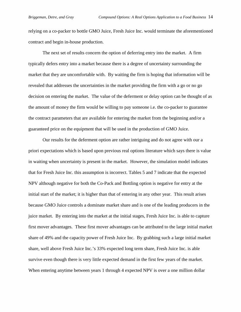
The next set of results concern the option of deferring entry into the market. A firm

typically defers entry into a market because there is a degree of uncertainty surrounding the

market that they are uncomfortable with. By waiting the firm is hoping that information will be

revealed that addresses the uncertainties in the market providing the firm with a go or no go

decision on entering the market. The value of the deferment or delay option can be thought of as

the amount of money the firm would be willing to pay someone i.e. the co-packer to guarantee

the contract parameters that are available for entering the market from the beginning and/or a

guaranteed price on the equipment that will be used in the production of GMO Juice.

Our results for the deferment option are rather intriguing and do not agree with our a

priori expectations which is based upon previous real options literature which says there is value

in waiting when uncertainty is present in the market. However, the simulation model indicates

that for Fresh Juice Inc. this assumption is incorrect. Tables 5 and 7 indicate that the expected

NPV although negative for both the Co-Pack and Bottling option is negative for entry at the

initial start of the market; it is higher than that of entering in any other year. This result arises

because GMO Juice controls a dominate market share and is one of the leading producers in the

juice market. By entering into the market at the initial stages, Fresh Juice Inc. is able to capture

first mover advantages. These first mover advantages can be attributed to the large initial market

share of 49% and the capacity power of Fresh Juice Inc. By grabbing such a large initial market

share, well above Fresh Juice Inc.’s 33% expected long term share, Fresh Juice Inc. is able

survive even though there is very little expected demand in the first few years of the market.

When entering anytime between years 1 through 4 expected NPV is over a one million dollar


loss, and only entering in year nine and ten does the expected NPV greater than entry at time

zero for the bottling option (Table 5). This occurs for two reasons: (1) the market has reached

maturity which creates a large and stable demand for the product and (2) Fresh Juice Inc. is able

sell off investments for a large salvage value. GMO Juice is unable to earn a positive NPV

because being a follower into the market GMO Juice enters below their long term market share,

i.e. they can not enter the market and automatically gain their market share, they must gradually

take market share away from the competition. The same results occur for the co-pack option

(Table 7).

The option value for deferment is negative for both the bottling and co-pack options until

the 9th and 10th year, when the option values are positive (Table 6 and 8). Furthermore, Fresh

Juice Inc. would never choose to enter the market because the NPV is still negative, even when

utilizing a deferment option. Although, if Fresh Juice Inc. was forced to enter or had already

make the commitment to contract with a co-packing company or purchased the equipment to

produce GMO Juice, they would wait to enter in year 10, which has the highest expected NPV.

The next option examined is the compound option, which is the combination of the

switching and delay option. It should be noted that a compound option, is not an additive option

i.e. one cannot simply add up the option values of the switching option and the deferment option

to get the value of the compound option. The compound option is dominated by the first mover

advantages associated with Fresh Juice Inc's market power and the switching option. Table 9

shows that the best time for GMO Juice to enter the market is at time zero. This where expected

NPV is $22,256 which is the same expected NPV as the switching option only. As with the

deferment option, it is observed that there are no advantages to waiting to enter the market for


Fresh Juice Inc., because of their dominant market position, however the ability to switch

production processes still maintains value.

Conclusions

Our results demonstrate that real options have value as a strategic proactive approach to

investment management, but it is not an analysis tool that is meant to be used blindly. The

results from our model indicate that there is value to having the ability to switch production

process i.e., Fresh Juice Inc. would be willing to pay to have flexibility in their production

process. However, the value of deferring entry is not valuable to Fresh Juice Inc. until year nine

or ten, because of the market position of Fresh Juice Inc. This result is in contrast to what is

often obtained through real options analysis using calculus which almost always indicates that

the value of waiting is positive when there is uncertainty in the market. By being able to capture

the effects of market power and first mover advantages in the simulation model, we have been

able to demonstrate that real options analysis has value but the value is not always positive as

traditional literature has indicated.

The real options analysis using simulation as a method to determine the true value of the

option is fruitful for further research. One possible extension of this research would be to

compare the results from the simulation model to that of a real options analysis that uses a

calculus based approach to solve for the values of the switching, delay, and compound options.

Another possible extension to this research would be to conduct real options analysis with other

data sets to test for the robustness of real options analysis conducted via simulation.

There are two key limitations to our research: the first is that we model supply as a

capacity system and that the firms can meet all demand market. These limitations are the result

of the data that was available for the model since the simulation model uses historical and


propriety information. The supply capacity is measured relative to Fresh Juice Inc. which is a

power of 1 and is not an actual capacity number for each firm.


References

Bernanke, B.S. “Irreversibility, Uncertainty, and Cyclical Investment.” Quarterly Journal of Economics. 98(February 1983):85-106. Copeland, T.E. and P.T. Keenan. “Making Real Options Real.” The McKinsey Quarterly. 3(1998):129-141. Dixit, A.K. “Entry and Exit Decisions under Uncertainty.” Journal of Political Economy. 97(June 1989):620-638. Dixit, A.K. and R.S. Pindyck. Investment Under Uncertainty. Princeton, NJ: Princeton University Press, 1994. Gray, A.W. Fresh Juice Inc.: Case Study. 2000. Hyde, J., J. Stokes, and P.D. Engel. “Optimal Investment in an Automatic Milking System: An Application of Real Options.” American Finance Review. 63(Spring 2003):75-92. McDonald, R. and D. Siegel. “The Value of Waiting to Invest.” Quarterly Journal of Economics. 101(November 1986):707-728. Mun, J. Real Options Analysis: Tools and Techniques for Valuing Strategic Investments and Decisions. Hoboken, NJ:John Wiley & Sons, 2002. Powell, S.G. “The Teacher’s Forum: From Intelligent Consumer to Active Modeler—Two MBA Success Stories.” Interfaces. 27(November/December 1997):88-98. Trigeorgis, L. “A Conceptual Options Framework for Capital Budgeting.” Advances in Futures and Options Research. 3(1988):145-168. ______. “A Log-Transformed Binomial Numerical Analysis Method for Valuing Complex Multi-Option Investments.” Journal of Financial and Quantitative Analysis. 26(September 1991):309-326. ______. “Anticipated Competitive Entry and Early Preemptive Investment in Deferrable Projects.” Journal of Economics and Business. 43(May 1991):143-156. ______. “The Nature of Option Interactions and the Valuation of Investments with Multiple Real Options.” Journal of Financial and Quantitative Analysis. 28(March 1993):1-20.

Bri

ggem

an, D

etre

, and

Gra

y

C

ompo

und

Opt

ions

: A

Rea

l Opt

ions

App

lica

tion

to a

Foo

d B

usin

ess

19

Tab

le 1

: H

isto

rica

l inf

orm

atio

n fo

r E

NE

R J

UIC

E

Tot

al A

nnua

l O

ur F

irm

's

Our

Fir

m's

N

umbe

r of

C

apac

ity/

Pow

er

Yea

r M

arke

t Sal

es

Sale

s Sh

are

Com

petit

ors

of a

ll C

ompe

titor

s P

rice

1985

42

9,88

5 42

9,88

5 1.

00

0 0.

00

2.88

19

86

719,

087

719,

087

1.00

0

0.00

3.

30

1987

97

0,38

0 97

0,38

0 1.

00

0 0.

00

3.62

19

88

1,04

9,53

7 1,

011,

850

0.96

1

0.27

2.

84

1989

1,

600,

187

1,45

1,47

7 0.

91

1 0.

27

2.73

19

90

1,78

8,93

3 1,

479,

509

0.83

2

0.52

2.

49

1991

1,

716,

579

1,26

4,33

3 0.

74

3 1.

12

1.55

19

92

1,58

5,35

9 1,

069,

566

0.67

3

1.12

1.

58

1993

1,

888,

628

1,19

3,08

8 0.

63

4 1.

48

1.46

19

94

1,68

9,30

9 89

2,34

4 0.

53

4 1.

48

1.49

19

95

1,65

4,92

0 84

6,66

8 0.

51

4 1.

48

1.64

19

96

998,

333

391,

218

0.39

5

2.03

1.

17

1997

1,

163,

044

447,

395

0.38

5

2.03

1.

31

1998

90

4,73

6 29

7,39

7 0.

33

5 2.

03

1.37

19

99

685,

750

226,

397

0.33

5

2.03

1.

49

Bri

ggem

an, D

etre

, and

Gra

y

C

ompo

und

Opt

ions

: A

Rea

l Opt

ions

App

lica

tion

to a

Foo

d B

usin

ess

20

Tab

le 2

: R

elat

ive

Pow

er o

f C

ompe

tito

rs a

nd P

roba

bilit

y of

Com

peti

tor

Ent

ry

R

elat

ive

Prob

abili

ty A

ssig

ned

to E

ntry

in Y

ear:

Fi

rm

Pow

er

1 2

3 4

5 1

0.27

0.

00

0.30

0.

60

0.90

1.

00

2 0.

25

0.00

0.

10

0.20

0.

30

0.40

3

0.60

1.

00

1.00

1.

00

1.00

1.

00

4 0.

36

0.00

0.

25

0.55

0.

75

1.00

5

0.55

0.

80

1.00

1.

00

1.00

1.

00

Tab

le 3

: N

PV

for

Bas

e Sc

enar

ios

and

the

Swit

chin

g O

ptio

n

B

ottl

ing

Co-

Pac

k Sw

itch

ing

Opt

ion

Stat

isti

cs

Net

Pre

sent

V

alue

N

et P

rese

nt

Val

ue

Net

Pre

sent

V

alue

M

ean

($54

0,63

5)

($44

,823

) $2

2,56

5

Stan

dard

D

evia

tion

$1

,297

,314

$1

,232

,898

$1

,262

,909

5%

($2,

495,

005)

($

1,90

5,13

0)

($1,

861,

560)

25

%

($1,

465,

734)

($

922,

617)

($

888,

854)

50

%

($65

3,56

3)

($14

8,96

0)

($89

,112

) 75

%

$292

,177

$7

65,0

14

$831

,268

95

%

$1,7

93,2

81

$2,1

92,8

65

$2,2

74,1

36

Bri

ggem

an, D

etre

, and

Gra

y

C

ompo

und

Opt

ions

: A

Rea

l Opt

ions

App

lica

tion

to a

Foo

d B

usin

ess

21

Tab

le 4

: V

alue

of

the

Swit

chin

g O

ptio

n fo

r th

e C

o-P

ack

and

Bot

tlin

g Sc

enar

io

Val

ue o

f t

he

Dif

fere

nce

of t

he

Sw

itch

ing

Opt

ion

Sw

itch

ing

Opt

ion

at t

he M

ean

fr

om a

Zer

o N

PV

B

ottl

ing

$5

63,2

00

$22,

565

C

o-P

ack

$67,

388

$2

2,56

5

Tab

le 5

: N

PV

for

the

Def

erm

ent

Opt

ion

Und

er t

he B

ottl

ing

Scen

ario

B

ottl

ing

Bot

tlin

g B

ottl

ing

Bot

tlin

g B

ottl

ing

Bot

tlin

g B

ottl

ing

Bot

tlin

g B

ottl

ing

Bot

tlin

g B

ottl

ing

N

et P

rese

nt

Val

ue

Net

Pre

sent

V

alue

N

et P

rese

nt

Val

ue

Net

Pre

sent

V

alue

N

et P

rese

nt

Val

ue

Net

Pre

sent

V

alue

N

et P

rese

nt

Val

ue

Net

Pre

sent

V

alue

N

et P

rese

nt

Val

ue

Net

Pre

sent

V

alue

N

et P

rese

nt

Val

ue

E

ntry

Yea

r M

ain

Mod

el

Mai

n M

odel

M

ain

Mod

el

Mai

n M

odel

M

ain

Mod

el

Mai

n M

odel

M

ain

Mod

el

Mai

n M

odel

M

ain

Mod

el

Mai

n M

odel

0

1 2

3 4

5 6

7 8

9 10

Mea

n ($

540,

635)

($

3,10

6,84

6)

($2,

984,

794)

($

2,44

5,96

1)

($1,

932,

314)

($

1,46

8,60

9)

($1,

086,

093)

($

776,

431)

($

543,

491)

($

329,

478)

($

134,

427)

Std

. Dev

$1

,297

,314

$7

62,3

61

$865

,498

$6

10,3

54

$437

,062

$3

22,3

03

$234

,862

$1

56,7

60

$91,

550

$4

3,17

2

$12,

982

5%

($2,

495,

005)

($

4,24

7,62

9)

($4,

560,

386)

($

3,48

9,73

2)

($2,

620,

826)

($

1,95

0,86

6)

($1,

434,

658)

($

1,00

7,45

4)

($67

6,90

3)

($39

2,37

8)

($15

3,67

2)

25%

($

1,46

5,73

4)

($3,

648,

234)

($

3,46

8,02

3)

($2,

851,

680)

($

2,25

1,69

2)

($1,

704,

023)

($

1,25

9,09

4)

($88

9,09

1)

($60

9,41

1)

($36

0,42

2)

($14

3,59

8)

50%

($

653,

563)

($

3,18

1,26

3)

($2,

893,

414)

($

2,42

6,87

2)

($1,

948,

156)

($

1,49

5,41

7)

($1,

107,

333)

($

791,

414)

($

551,

591)

($

333,

562)

($

135,

555)

75%

$2

92,1

77

($2,

613,

721)

($

2,41

0,99

1)

($2,

037,

345)

($

1,65

0,94

4)

($1,

265,

609)

($

941,

522)

($

680,

858)

($

488,

283)

($

303,

666)

($

126,

703)

95%

$1

,793

,281

($

1,75

0,92

9)

($1,

680,

224)

($

1,46

1,12

5)

($1,

174,

872)

($

898,

623)

($

661,

943)

($

492,

888)

($

376,

517)

($

250,

192)

($

111,

002)

Bri

ggem

an, D

etre

, and

Gra

y

C

ompo

und

Opt

ions

: A

Rea

l Opt

ions

App

lica

tion

to a

Foo

d B

usin

ess

22

Tab

le 6

: V

alue

of

the

Def

erm

ent

Opt

ion

Und

er t

he B

ottl

ing

Scen

ario

V

alue

of

the

V

alue

of

the

Def

erm

ent

Opt

ion

D

efer

men

t O

ptio

n

at

the

Mea

n

at t

he M

ean

B

ottl

ing

Yea

r 0

$0

($54

0,63

5)

Bot

tlin

g Y

ear

1 ($

2,56

6,21

1)

($3,

106,

846)

B

ottl

ing

Yea

r 2

($2,

444,

160)

($

2,98

4,79

4)

Bot

tlin

g Y

ear

3 ($

1,90

5,32

6)

($2,

445,

961)

B

ottl

ing

Yea

r 4

($1,

391,

679)

($

1,93

2,31

4)

Bot

tlin

g Y

ear

5 ($

927,

974)

($

1,46

8,60

9)

Bot

tlin

g Y

ear

6 ($

545,

459)

($

1,08

6,09

3)

Bot

tlin

g Y

ear

7 ($

235,

797)

($

776,

431)

B

ottl

ing

Yea

r 8

($2,

856)

($

543,

491)

B

ottl

ing

Yea

r 9

$211

,156

($

329,

478)

B

ottl

ing

Yea

r 10

$4

06,2

08

($13

4,42

7)

Tab

le 7

: N

PV

for

the

Def

erm

ent

Opt

ion

Und

er t

he C

o-P

ack

Scen

ario

C

o-P

ack

Co-

Pac

k C

o-P

ack

Co-

Pac

k C

o-P

ack

Co-

Pac

k C

o-P

ack

Co-

Pac

k C

o-P

ack

Co-

Pac

k C

o-P

ack

N

et P

rese

nt

Val

ue

Net

Pre

sent

V

alue

N

et P

rese

nt

Val

ue

Net

Pre

sent

V

alue

N

et P

rese

nt

Val

ue

Net

Pre

sent

V

alue

N

et P

rese

nt

Val

ue

Net

Pre

sent

V

alue

N

et P

rese

nt

Val

ue

Net

Pre

sent

V

alue

N

et P

rese

nt

Val

ue

E

ntry

Yea

r M

ain

Mod

el

Mai

n M

odel

M

ain

Mod

el

Mai

n M

odel

M

ain

Mod

el

Mai

n M

odel

M

ain

Mod

el

Mai

n M

odel

M

ain

Mod

el

Mai

n M

odel

0

1 2

3 4

5 6

7 8

9 10

Mea

n ($

44,8

23)

($2,

103,

905)

($

1,80

1,50

3)

($1,

398,

532)

($

1,00

4,14

4)

($65

5,93

7)

($38

9,38

5)

($20

1,29

2)

($10

2,74

9)

($41

,651

) ($

11,0

47)

Std.

Dev

$1

,232

,898

$7

28,3

59

$870

,216

$6

03,7

89

$429

,892

$3

16,2

60

$230

,530

$1

54,3

47

$90,

706

$4

3,02

9

$13,

000

5%

$0

($3,

205,

236)

($

3,43

8,84

1)

($2,

455,

703)

($

1,70

7,94

9)

($1,

141,

984)

($

738,

838)

($

434,

796)

($

239,

188)

($

106,

252)

($

30,1

06)

25%

$3

($

938,

540)

($

938,

540)

($

938,

540)

($

938,

540)

($

938,

540)

($

938,

540)

($

938,

540)

($

938,

540)

($

938,

540)

($

938,

540)

50%

$0

($

2,15

0,73

3)

($1,

664,

903)

($

1,35

0,21

3)

($1,

007,

633)

($

671,

936)

($

401,

761)

($

211,

156)

($

110,

083)

($

45,2

67)

($12

,338

)

75%

($

527,

420)

($

1,64

2,43

7)

($1,

217,

571)

($

990,

031)

($

715,

496)

($

452,

375)

($

241,

801)

($

104,

776)

($

47,6

73)

($15

,814

) ($

3,33

9)

95%

($

1,90

5,13

0)

($84

0,22

1)

($54

6,42

1)

($44

6,61

2)

($28

2,74

9)

($10

4,81

8)

$21,

738

$7

4,68

0

$59,

048

$3

6,45

6

$12,

629

Bri

ggem

an, D

etre

, and

Gra

y

C

ompo

und

Opt

ions

: A

Rea

l Opt

ions

App

lica

tion

to a

Foo

d B

usin

ess

23

Tab

le 8

: V

alue

of

the

Def

erm

ent

Opt

ion

for

the

Co-

Pac

k Sc

enar

io

Val

ue o

f th

e

Dif

fere

nce

of t

he

D

efer

men

t O

ptio

n

Def

erm

ent

Opt

ion

at t

he M

ean

fr

om a

Zer

o N

PV

B

ottl

ing

Yea

r 0

$0

($44

,823

) B

ottl

ing

Yea

r 1

($2,

059,

082)

($

2,10

3,90

5)

Bot

tlin

g Y

ear

2 ($

1,75

6,68

0)

($1,

801,

503)

B

ottl

ing

Yea

r 3

($1,

353,

709)

($

1,39

8,53

2)

Bot

tlin

g Y

ear

4 ($

959,

321)

($

1,00

4,14

4)

Bot

tlin

g Y

ear

5 ($

611,

114)

($

655,

937)

B

ottl

ing

Yea

r 6

($34

4,56

2)

($38

9,38

5)

Bot

tlin

g Y

ear

7 ($

156,

469)

($

201,

292)

B

ottl

ing

Yea

r 8

($57

,926

) ($

102,

749)

B

ottl

ing

Yea

r 9

$3,1

72

($41

,651

) B

ottl

ing

Yea

r 10

$3

3,77

6

($11

,047

)

Tab

le 9

: N

PV

for

the

Com

poun

d O

ptio

n

Sw

itch

ing

Swit

chin

g Sw

itch

ing

Swit

chin

g Sw

itch

ing

Swit

chin

g Sw

itch

ing

Swit

chin

g Sw

itch

ing

Swit

chin

g Sw

itch

ing

N

et P

rese

nt

Val

ue

Net

Pre

sent

V

alue

N

et P

rese

nt

Val

ue

Net

Pre

sent

V

alue

N

et P

rese

nt

Val

ue

Net

Pre

sent

V

alue

N

et P

rese

nt

Val

ue

Net

Pre

sent

V

alue

N

et P

rese

nt

Val

ue

Net

Pre

sent

V

alue

N

et P

rese

nt

Val

ue

E

ntry

Yea

r M

ain

Mod

el

Mai

n M

odel

M

ain

Mod

el

Mai

n M

odel

M

ain

Mod

el

Mai

n M

odel

M

ain

Mod

el

Mai

n M

odel

M

ain

Mod

el

Mai

n M

odel

Stat

isti

cs

0 1

2 3

4 5

6 7

8 9

10

Mea

n $2

2,56

5

($2,

136,

428)

($

1,91

8,35

0)

($1,

748,

708)

($

1,49

2,36

9)

($1,

238,

411)

($

1,03

4,19

5)

($88

1,43

2)

($78

8,28

7)

($73

6,12

8)

($71

1,91

9)

Stan

dard

D

evia

tion

$1

,262

,909

$7

35,7

31

$871

,241

$6

06,0

56

$433

,532

$3

18,1

62

$234

,745

$1

56,3

15

$90,

730

$4

3,02

9

$13,

000

5%

$0

($3,

247,

318)

($

3,54

1,19

6)

($2,

822,

698)

($

2,20

0,17

1)

($1,

728,

574)

($

1,40

0,11

6)

($1,

123,

804)

($

924,

984)

($

800,

729)

($

730,

978)

25%

$3

($

2,65

7,87

5)

($2,

365,

504)

($

2,13

2,23

2)

($1,

799,

917)

($

1,46

3,54

0)

($1,

199,

381)

($

991,

988)

($

852,

979)

($

766,

791)

($

721,

186)

50%

$0

($

2,19

0,22

5)

($1,

799,

669)

($

1,71

3,42

9)

($1,

498,

394)

($

1,25

4,41

6)

($1,

047,

199)

($

889,

917)

($

795,

570)

($

739,

743)

($

713,

211)

75%

$8

1,61

4

($1,

668,

428)

($

1,33

9,03

2)

($1,

341,

094)

($

1,20

3,74

4)

($1,

034,

976)

($

885,

336)

($

781,

166)

($

733,

288)

($

710,

291)

($

704,

211)

95%

($

1,86

1,56

0)

($81

6,70

0)

($65

1,34

7)

($76

6,50

4)

($76

2,77

9)

($69

4,01

5)

($62

1,63

6)

($60

5,78

8)

($62

6,43

8)

($65

8,02

1)

($68

8,24

4)

Bri

ggem

an, D

etre

, and

Gra

y

C

ompo

und

Opt

ions

: A

Rea

l Opt

ions

App

lica

tion

to a

Foo

d B

usin

ess

24

µ 1

µ 2

Tab

le 1

0: V

alue

of

the

Com

poun

d O

ptio

n

Val

ue o

f th

e

Dif

fere

nce

of t

he

C

ompo

und

Opt

ion

C

ompo

und

Opt

ion

at t

he M

ean

fr

om a

Zer

o N

PV

B

ottl

ing

Yea

r 0

$67,

388

$2

2,56

5

Bot

tlin

g Y

ear

1 ($

2,09

1,60

5)

($2,

136,

428)

B

ottl

ing

Yea

r 2

($1,

873,

527)

($

1,91

8,35

0)

Bot

tlin

g Y

ear

3 ($

1,70

3,88

5)

($1,

748,

708)

B

ottl

ing

Yea

r 4

($1,

447,

546)

($

1,49

2,36

9)

Bot

tlin

g Y

ear

5 ($

1,19

3,58

8)

($1,

238,

411)

B

ottl

ing

Yea

r 6

($98

9,37

2)

($1,

034,

195)

B

ottl

ing

Yea

r 7

($83

6,60

9)

($88

1,43

2)

Bot

tlin

g Y

ear

8 ($

743,

464)

($

788,

287)

B

ottl

ing

Yea

r 9

($69

1,30

5)

($73

6,12

8)

Bot

tlin

g Y

ear

10

($66

7,09

6)

($71

1,91

9)

P

roba

bilit

y

R

eal O

ptio

ns

D

CF

App

roac

h

Sour

ce:

Mun

F

igur

e 1.

DC

F a

nd R

eal O

ptio

ns:

Ris

k-R

etur

n C

ompa

riso

ns

% R

etur

ns

σ 1

σ 2

Documents

COMPOUND OPTIONS: A REAL OPTIONS APPLICATION TO …ageconsearch.umn.edu/bitstream/19996/1/sp04br02.pdf · Briggeman, Detre, and Gray Compound Options: A Real Options Application to