Compositional Neural-Network Modeling ofComplex Analog Circuits

Ramin M. Hasani∗, Dieter Haerle∗∗, Christian F. Baumgartner§, Alessio R. Lomuscio§ and Radu Grosu∗∗Institute of Computer Engineering, Vienna University of Technology, Austria

(ramin.hasani, radu.grosu) @tuwien.ac.at∗∗KAI Kompetenzzentrum Automobil- und Industrieelektronik GmbH, Villach, Austria

dieter.haerle @k-ai.at§Department of Computing, Imperial College London, UK

(c.baumgartner, a.lomuscio) @imperial.ac.uk

Abstract—We introduce CompNN, a compositional method forthe construction of a neural-network (NN) capturing the dynamicbehavior of a complex analog multiple-input multiple-output(MIMO) system. CompNN first learns for each input/outputpair (i, j), a small-sized nonlinear auto-regressive neural networkwith exogenous input (NARX) representing the transfer-functionhij . The training dataset is generated by varying input i of theMIMO, only. Then, for each output j, the transfer functions hij

are combined by a time-delayed neural network (TDNN) layer, fj .The training dataset for fj is generated by varying all MIMOinputs. The final output is f =(f1, . . ., fn). The NNs parame-ters are learned using Levenberg-Marquardt back-propagationalgorithm. We apply CompNN to learn an NN abstraction of aCMOS band-gap voltage-reference circuit (BGR). First, we learnthe NARX NNs corresponding to trimming, load-jump and line-jump responses of the circuit. Then, we recompose the outputsby training the second layer TDNN structure. We demonstratethe performance of our learned NN in the transient simulationof the BGR by reducing the simulation-time by a factor of 17compared to the transistor-level simulations. CompNN allows usto map particular parts of the NN to specific behavioral featuresof the BGR. To the best of our knowledge, CompNN is the firstmethod to learn the NN of an analog integrated circuit (MIMOsystem) in a compositional fashion.

I. INTRODUCTION

One challenging issue in the pre-silicon verification processof recently produced analog integrated circuits (IC)s is the de-velopment of high performance models for carrying out time-efficient simulations. Transistor-level fault simulations of a sin-gle analog IC can take up to one or two weeks to be completed.As a result, over the past years, several attempts to develop fastbehavioral models of the analog ICs have been investigated.Examples include SystemC, Verilog HDL, Verilog AMS andVerilog-A models which in principle can realize very accuratemodels [1]–[4]. However, the development of such models isnot automated, and the associated human effort is considerable[1]. Moreover, this approach is unlikely to scale up to largelibraries of existing analog components. Another example isreal number modeling (RNM). In this method, analog partsof a mixed-signal IC are functionally modeled by real valuesand they are used in top-level system on chip verification [5].RNMs are fast and cover a large range of circuits. However, foranalog circuits including continuous time feedbacks or detailedRC filter effects, it is not recommended [5]. Moreover, RNM

is not appropriate to be employed for circuits that are sensitiveto nonlinear input-output (I/O) impedance interaction.

In this paper we propose an alternative machine-learningapproach for automatically deriving neural network (NN)abstractions of integrated circuits, up to a prescribed toleranceof the behavioral features. NN modeling of the electroniccircuits has been recently used in electromagnetic compat-ibility (EMC) testing, where the authors modeled a band-gap reference circuit (BGR) by utilizing an echo-state neuralnetwork [6]. The developed NN model has shown a reasonabletime performance in transient simulations; however, since themodel is coded in Verilog-A, simulation speed-up is limited.In [7], authors used a novel nonlinear autoregressive neural-network with exogenous input (NARX) for modeling thepower-up behavior of a BGR. They demonstrated attractiveimprovements in the time performance of the transient simu-lations of the analog circuit within the Cadence AMS simulatorby using this NARX model.

In the present study, we employ a compositional approachfor learning the Overall time-domain behavior of a complexmultiple-input multiple-output (MIMO) system, CompNN.CompNN learns in a first step, for each input i and eachoutput j a small-sized nonlinear auto-regressive NNs withexhogeneous inputs (NARX) representing the transfer-functionfiJ from i to j. The learning data-set for hij is generated byvarying only input i of the MIMO system and keeping allthe other inputs constant. In a second step, for each outputj, the transfer functions hij learned in Step 1, one for eachinput i, are combined by a (possibly nonlinear) function fj ,which is learned by employing another NN layer. The trainingdataset in this case is generated by applying all the inputs atthe same time to the MIMO system. Once we constructedfj for each output j, the overall output function is obtainedas f =(f1, . . ., fn). We evaluate our approach by modelingthe main time-domain behavioral features of a CMOS band-gap voltage reference circuit. We initially extract such featuresfrom the BGR circuit by using our I/O decomposition method.Consequently, we define trimming, load jump and line jump asthe main behavioral features of the circuit to be modeled. Indi-vidual small-sized NARX networks are designed and trained inorder to model the BGR output responses. We recompose the

trained models by stacking a second layer network in a time-delayed neural network (TDNN) structure. The second layer isthen trained in order to reproduce the output of the BGR. Suchimplementation provides us with an observable model whereone can define a one-to-one mapping from specific behavioralfeatures of the system to certain parts of the model. Finally,we employ our neural network model in a transient simulationof the BGR and evaluate its performance. This is done byutilizing a co-simulation approach between MATLAB andCadence AMS Designer environment [8]. We demonstrate thatby using such 2-layer neural network structure, we can achieveone order of magnitude speed-up in the transient simulations.

The rest of the paper is organized as follows. In sectionII, we introduce our compositional approach for developingneural network models and define the case study. In SectionIII, we describe the NARX neural network architecture andidentify the optimal quantity of components to be used inthe neural network for each behavioral response. In SectionIV, we explain the training process performed on the networkand explore the performance of the designed models. Sub-sequently, in Section V, we train the second layer with theaim of merging the behavioral models into a single block.Finally, in Section VI, we employ a co-simulation approach forsimulating our MATLAB/Simulink neural network model intoCadence Design environment and illustrate the performanceof the network.

II. COMPNN FOR MIMO SYSTEM MODELING

Let I = {i1, i2, ..., in} be the vector of the defined inputsto a MIMO system, and H = {h1, h2, ..., hm} be the vectorof nonlinear transfer functions delivering the correspondingoutput for each input exclusively, each output of the systemis then constructed as O = f(O1, O2, ..., Om) where f,depending on the device under test (DUT), can be a linearor nonlinear function. As a result, we train small-sized neuralnetworks for modeling each component of vector H andsubsequently we estimate the function f for merging suchcomponents by a second layer NN. We call such compositionalapproach CompNN. CompNN provides us with the abilityof mapping particular parts of the neural network model tospecific behavioral features of the DUT and therefore havingan observable model.

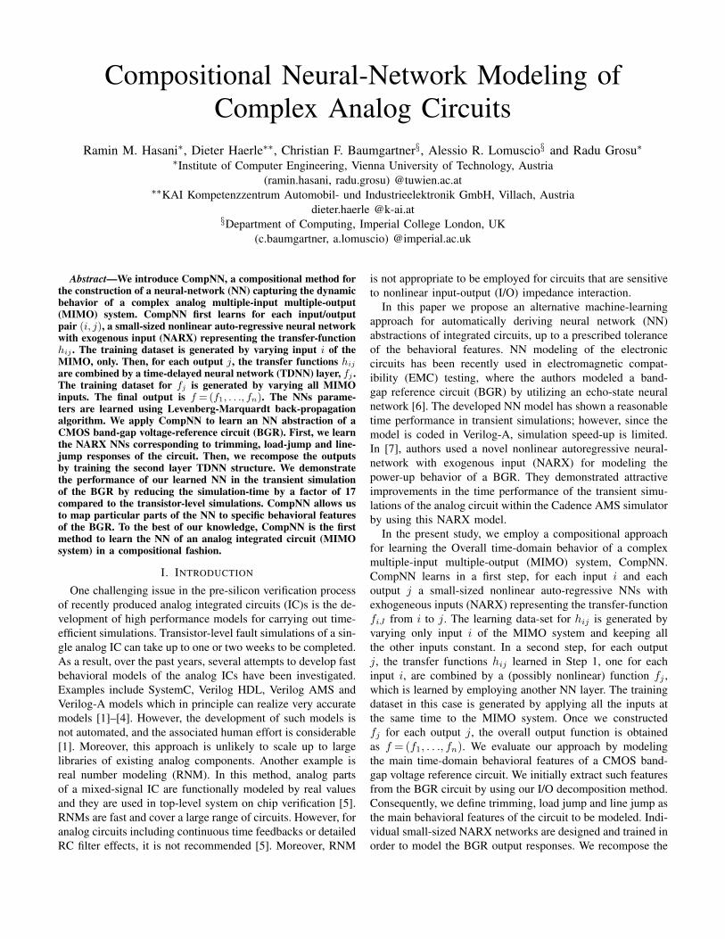
We demonstrate the performance of our method by devel-oping a NN behavioral model of an analog integrated circuit:CMOS band-gap voltage reference circuit (BGR). A BGR out-puts constant voltages (in our case 1V and 0.49V) regardlessof possible variations caused by temperature change, powersupply and load properties. Figure 1A depicts a symbolicrepresentation of our BGR. The circuit is constructed from 50transistors. We define the inputs to the system to be the powersupply (VDD) and three digital trimming inputs. A load-profilecan be applied to the output-pin of the circuit (1V-Out). Wetherefore consider the load-profile as an input signal as well.Thus, the circuit realizes a multi-input single-output (MISO)dynamic system which is a particular case of a MIMO system.

Figure 1B shows the BGR behavioral representation wherethe circuit comprises several behavioral features such as:

Power-up – which is the activation of the power supply withseveral slopes and voltage levels.

Trimming inputs – which enables the circuit to generate 8different stable outputs between 0.9 and 1.1 on its 1V-outputpin. There are three digital trimming inputs.

Load jump – demonstrates the variations occurred on theoutput voltage when a current load is applied.

Line jump – models the response of the BGR when there isa line jump on the power supply of the circuit.

Features are consequently recomposed by the function fand create the output of the circuit.

In [7], authors employed a NARX NN for modeling thepower-up behavior of the BGR. In this paper we model the restof the decomposed features and thus complete the behavioralmodeling of the circuit. We merge the behavioral featuresby approximating the function f using a second layer, time-delayed neural network.

Fig. 1. CMOS band-gap voltage reference circuit (BGR) A) Symbolicrepresentation of the circuit schematic. B) Behavioral representation of thecircuit.

III. NARX NEURAL-NETWORK ARCHITECTURE

Although the transfer function of a BGR is in principleconstant, this is in practice highly nonlinear. As a conse-

quence, modeling of the time-domain features requires pow-erful nonlinear system identification techniques and solutions.A nonlinear auto-regressive neural network with exogenousinput (NARX NN) appears to be a suitable framework forderiving approximations, up to a prescribed, maximum error,of the BGR. It has been previously demonstrated that arecurrent nature of the NARX NN topology consisting of onlyseven neurons and three three-time input-and-output delaycomponents is able to precisely reproduce the turn-on behaviorof the circuit [7].

In this paper, we use the NARX architecture for modelingin addition the trimming, load jump and line jump behaviorsof the BGR. The output of the network is constructed from thetime-delayed components of the input signal X(t) and outputsignal Y (t), (see for example [9]):

Y (t) = f(X(t− 1), X(t− 2), ..., X(t− nx),

Y (t− 1), Y (t− 2), ..., Y (t− ny)).(1)

The nx and the ny factors, define the input and output delays,that is, the number of discrete time steps within the input andthe output histories that the component has to remember, inorder to properly predict the next value of the output [10].n = nx + ny is the number of input nodes.

The size of the hidden layer is highly dependent on the num-ber of the input nodes. There are several ad-hoc approachesfor defining the appropriate number of hidden neurons. Forinstance one of the popular methods prescribes that the numberof neurons within the hidden layer should be between thenumber of input nodes [11] and output nodes. We performa grid search for choosing the optimal number of the delaycomponents and hidden layer neurons [12]. A hyperparameterspace (d, h), consists of two parameters representing the quan-tity of delay components d, and the number of hidden-layerneurons h. Parameter d is chosen from a set D = {1, 2, ..., 7}and h from the set H = {1, 2, ..., 15}. The Levenberg-Marquardt back propagation is performing a parameter opti-mization where the error of the validation dataset for eacharchitecture pair (d, h), is calculated in the course of thetraining process. We ultimately select the architecture pairwhich results in the least validation error. Table I depictsthe optimal number of delay components and hidden neuronschosen for realization of individual BGR features. As the

TABLE INARX NETWORK ARCHITECTURE FOR EACH OF THE BGR BEHAVIORAL

FEATURES

Features ♯ of delay components ♯ of hidden neuronsTrimming 3 10

Load Jump 3 7

Line Jump 3 7

output layer is a regressor, it comprises only one node.The NARX architecture therefore, is designed for each

behavioral task as shown in Figure 2. In this architecture,weighted input components synapse into the hidden layernodes with an all-to-all connection topology. We evaluated

Fig. 2. NARX neural network architecture. Note that the network realizesa recurrent topology where the output is fed-back into the input layer andcauses further refinements on the predicted output signal Y 1.

TABLE IITRANSIENT SIMULATIONS PERFORMED FOR THE TRAINING DATA

COLLECTION PURPOSES

Simulation Simulation Time CPU time Input Output ♯ of samples

Trimming 100 µs 1.4 s Trimming inputs V out1V 695

Load Jump 540 µs 1.3 s Load Profile V out1V 433

Line Jump 200 µs 1 s VDD V out1V 501

different activation functions such as (Elliot, logistic sigmoidand tanh) and achieved the best performance by using ahyperbolic-tangent activation-function:

H = tanh(N∑

i,j=1

(wijXi) + bj), (2)

where H is the output of the hidden layer, wij represents thesynaptic weight of the input Xi, from input node i to hiddennode j and bj depicts the bias weight applied to the hiddenneuron j. The output of the NARX network is constructed as alinear sum of the weighted Hidden layer outputs. The networkis designed in MATLAB [13].

IV. TRAINING PROCESS AND NETWORK PERFORMANCE

In order to collect adequate training datasets for teaching theNARX networks for the three behavioral features of the BGRthat is, trimming, load jump and line jump, we perform threetransient simulations on the BGR by using the AMS simulatorwithin the Cadence environment. Table II shows the details ofthe performed simulations and the collected datasets.

We aim to train a specific NARX network for each of the be-havioral features where we use the input data as the exogenousinput to the neural network and the output data as the targetvalues to be learned. In order to gain high precision in thetraining process, we use the network in a feedforward topologyin which the input of this topology consists of the originalinputs and outputs, plus all the delayed inputs and outputs, upto their maximum input and output delays, respectively [7].A Levenberg-Marquardt (LM) back-propagation algorithm isemployed for training each network [14]. The LM learning

0.6

0.8

1

1.2

1.4O

utp

ut

an

d T

arg

et

100 200 300 400Samples

-0.2

0

0.2

Err

or Targets - Outputs

0 10 20 3032 Epochs

10-4

10-2

100

Mean

Sq

uare

d E

rro

r (m

se) Train

ValidationTestBest

0

200

400

600

Ins

tan

ce

s

-0.2

359

-0.1

769

-0.1

18

-0.0

59

-7.6

e-0

5

0.0

58

0.1

178

0.1

768

0.2

357

0.2

947

Errors = Targets - Outputs

TrainingValidationTestZero Error

0 5 10 15 2023 Epochs

10-4

10-2

100

Mean

Sq

uare

d E

rro

r (m

se)

TrainValidationTestBest

0 5 10 1516 Epochs

10-4

10-2

100

Mean

Sq

uare

d E

rro

r (m

se) Train

ValidationTestBest

-0.5

-0.4

-0.3

-0.2

-0.1

0.1

0.2

0.3

0.4

0.5

0

100

200

300

400

Insta

nces

0.0

05

6

Errors = Targets - Outputs

TrainingValidationTestZero Error

-0.5

-0.4

-0.3

-0.2

-0.1

0.1

0.2

0.3

0.4

0.5

0

100

200

300

400

500

Ins

tan

ce

s

-0.0

14

Errors = Targets - Outputs

TrainingValidationTestZero Error

A B

D E

C

F

G H I

0.99

0.995

1

1.005

1.01

Ou

tpu

t an

d T

arg

et

100 200 300 400Samples

-5

0

5

Err

or

× 10-3

Targets - Outputs

0

0.2

0.4

0.6

0.8

1

1.2

Ou

tpu

t an

d T

arg

et

Training TargetsTraining OutputsValidation TargetsValidation OutputsTest TargetsTest OutputsErrorsResponse

200 400 600Samples

-0.1

0

0.1

Err

or Targets - Outputs

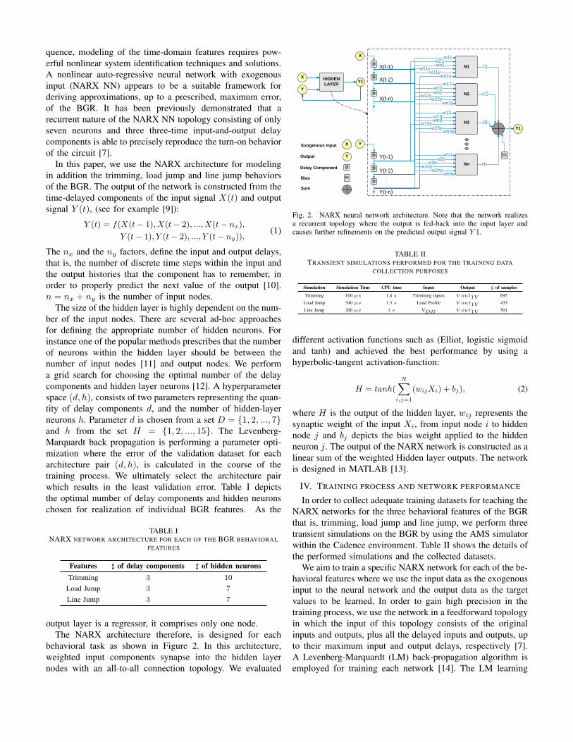
Fig. 3. Network performance of the trimming, load jump and line jump NARX behavioral models. A, B and C display the performance of the NARX neuralnetwork model of trimming, load jump and line jump, respectively, throughout the training process. The MSE is reduced drastically by each training step.In all three cases, the process terminated as soon as the validation dataset error stopped descending after 6 consequent epochs. D, E and F shows the errorhistogram of training samples for the NARX model of trimming, load jump and line jump behavior, respectively. Note that most of the instances’ error areclose to the zero error line for each case. G, H and I represent the output of the band-gap circuit together with its neural network response for trimming, loadjump and line jump behaviors, respectively. They also show the generated output error per sample.

method, which is a modified version of the Gauss-Newtontraining algorithm, results in fast convergence of the gradientto its minimum since it is unaccompanied by calculation ofHessian matrix. We initially define a cost function as follows:

E(w, b) =1

2

∑k∈K

(f(w, b)k − tk)2, (3)

where E(w, b) stands for the error rate as a function of theweight w, and bias values b, f(w, b)k is the output generatedby the neural network and tk is the target outputs. We thentry to minimize the error function for each training iterationwith respect to the synaptic weights. △w which is calculatedby the LM method and it is given by:

△w = [JT (w)J(w) + ηI]−1JT (w)(f(w)− t), (4)

Accordingly, the updated value of the weights is computed as:

wnew = w +△w. (5)

where J(w) is the Jacobian matrix comprising the first-orderderivatives of the error function with respect to weight values.

Parameter η is the key to the fast convergence [15]. When thisparameter is zero, the LM method realizes the common Gauss-Newton algorithm. If η increases throughout the trainingprocess, it is multiplied by an ηincrease value. On the contrary,when a training step results in a decrease of the value of η,its value gets reduced by a ηdecrease value. As a result, thecost function moves in a fast way towards the error reductionwithin each training epoch. The parameters’ initial values anddescriptions employed within the LM training algorithm aresummarized in the Table III.

For starting the training process, the collected samples arerandomly divided into three data subsets consisting of:

• Training set (70%): This dataset is employed during thetraining process.

• Validation set (15%): This dataset is used for generaliza-tion and validation purposes. It also plays a role in thetermination of the training process.

• Test set (15%): This dataset provides an additional eval-uation test after the training phase. It is not deployed

-20 -10 0 10 20

Lag

-0.5

0

0.5

1

1.5

2

2.5

3

Co

rrela

tio

n

× 10-3

Correlations

Zero Correlation

Confidence Limit

0.9 0.95 1 1.05 1.1

Target

0.9

0.95

1

1.05

1.1

Ou

tpu

t ~

= 0

.99

*Ta

rge

t +

0.0

05

8 R=0.99834Data

Fit

Y = T

1 1.05 1.1 1.15 1.2

Target

1

1.05

1.1

1.15

1.2

Ou

tpu

t ~

= 0

.82

*Ta

rge

t +

0.1

9 R=0.96009Data

Fit

Y = T

0.995 1 1.005 1.01

Target

0.99

0.995

1

1.005

1.01

Ou

tpu

t ~

= 0

.91

*Ta

rge

t +

0.0

82 R=0.96912Data

Fit

Y = T

-20 -10 0 10 20

Lag

-1

0

1

2

3

Co

rrela

tio

n× 10

-4

Correlations

Zero Correlation

Confidence Limit

-20 -10 0 10 20

Lag

0

5

10

15

Co

rrela

tio

n

× 10-4

Correlations

Zero Correlation

Confidence Limit

A B C

D E F

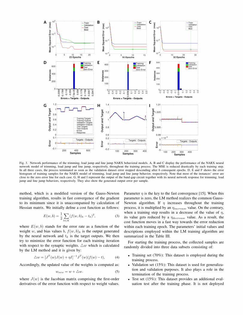
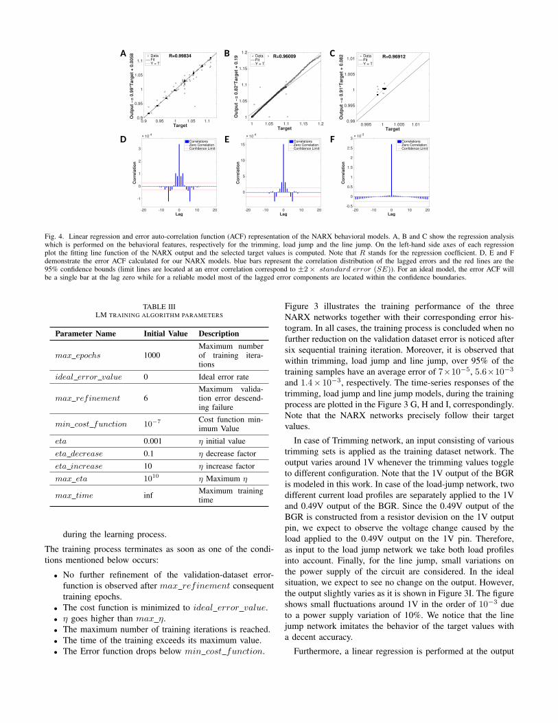
Fig. 4. Linear regression and error auto-correlation function (ACF) representation of the NARX behavioral models. A, B and C show the regression analysiswhich is performed on the behavioral features, respectively for the trimming, load jump and the line jump. On the left-hand side axes of each regressionplot the fitting line function of the NARX output and the selected target values is computed. Note that R stands for the regression coefficient. D, E and Fdemonstrate the error ACF calculated for our NARX models. blue bars represent the correlation distribution of the lagged errors and the red lines are the95% confidence bounds (limit lines are located at an error correlation correspond to ±2× standard error (SE)). For an ideal model, the error ACF willbe a single bar at the lag zero while for a reliable model most of the lagged error components are located within the confidence boundaries.

TABLE IIILM TRAINING ALGORITHM PARAMETERS

Parameter Name Initial Value Description

max epochs 1000Maximum numberof training itera-tions

ideal error value 0 Ideal error rate

max refinement 6Maximum valida-tion error descend-ing failure

min cost function 10−7 Cost function min-imum Value

eta 0.001 η initial value

eta decrease 0.1 η decrease factor

eta increase 10 η increase factor

max eta 1010 η Maximum η

max time inf Maximum trainingtime

during the learning process.

The training process terminates as soon as one of the condi-tions mentioned below occurs:

• No further refinement of the validation-dataset error-function is observed after max refinement consequenttraining epochs.

• The cost function is minimized to ideal error value.• η goes higher than max η.• The maximum number of training iterations is reached.• The time of the training exceeds its maximum value.• The Error function drops below min cost function.

Figure 3 illustrates the training performance of the threeNARX networks together with their corresponding error his-togram. In all cases, the training process is concluded when nofurther reduction on the validation dataset error is noticed aftersix sequential training iteration. Moreover, it is observed thatwithin trimming, load jump and line jump, over 95% of thetraining samples have an average error of 7×10−5, 5.6×10−3

and 1.4× 10−3, respectively. The time-series responses of thetrimming, load jump and line jump models, during the trainingprocess are plotted in the Figure 3 G, H and I, correspondingly.Note that the NARX networks precisely follow their targetvalues.

In case of Trimming network, an input consisting of varioustrimming sets is applied as the training dataset network. Theoutput varies around 1V whenever the trimming values toggleto different configuration. Note that the 1V output of the BGRis modeled in this work. In case of the load-jump network, twodifferent current load profiles are separately applied to the 1Vand 0.49V output of the BGR. Since the 0.49V output of theBGR is constructed from a resistor devision on the 1V outputpin, we expect to observe the voltage change caused by theload applied to the 0.49V output on the 1V pin. Therefore,as input to the load jump network we take both load profilesinto account. Finally, for the line jump, small variations onthe power supply of the circuit are considered. In the idealsituation, we expect to see no change on the output. However,the output slightly varies as it is shown in Figure 3I. The figureshows small fluctuations around 1V in the order of 10−3 dueto a power supply variation of 10%. We notice that the linejump network imitates the behavior of the target values witha decent accuracy.

Furthermore, a linear regression is performed at the output

100 200 300 400 500 600Samples

0

1

2

3

4

5

6

Trim

min

g Inputs

(V

)

Trimming Input 1 (T1)Trimming input 2 (T2)Trimming input 3 (T3)

100 010 001110 111011101

000

T3 T2 T1

100 200 300 400 500 600Samples

0

2

4

6

8

Load P

rofile

(µ

A)

Load Applied to the 0.49V OutputLoad Applied to the 1V Output

A B C

200 400 600Samples

0

1

2

3

4

5

6

Trim

min

g I

np

uts

(V

)

Trimming Input 1 (T1)Trimming Input 2 (T2)Trimming Input 3 (T3)

000

011010101100 111110001

T3 T2 T1

200 400 600Samples

0

1

2

3

4

5

6

Trim

min

g I

np

uts

(V

)

Trimming Input 1 (T1)Trimming Input 2 (T2)Trimming Input 3 (T3)

100 011 111

000

011 101 010 110

T3 T2 T1

100 200 300 400 500 600Samples

0

2

4

6

8

Load P

rofil

e (µ

A)

Load Applied to the 0.49V OutputLoad Applied to the 1V Output

D E F

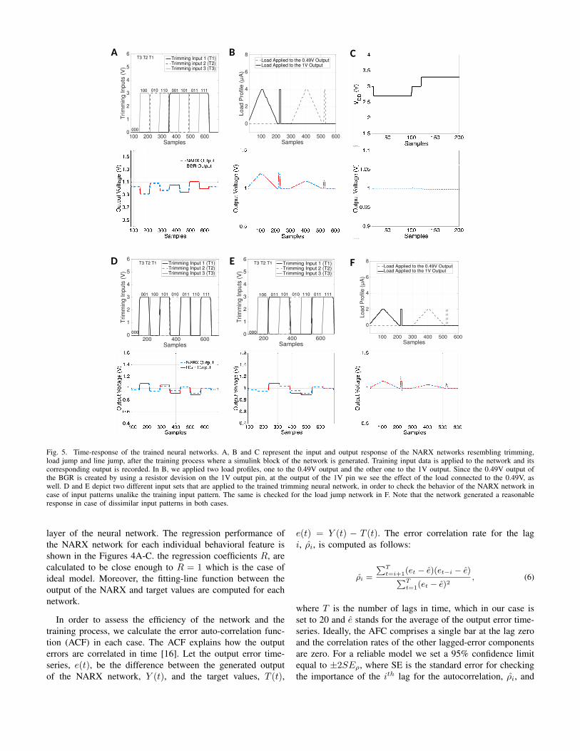
Fig. 5. Time-response of the trained neural networks. A, B and C represent the input and output response of the NARX networks resembling trimming,load jump and line jump, after the training process where a simulink block of the network is generated. Training input data is applied to the network and itscorresponding output is recorded. In B, we applied two load profiles, one to the 0.49V output and the other one to the 1V output. Since the 0.49V output ofthe BGR is created by using a resistor devision on the 1V output pin, at the output of the 1V pin we see the effect of the load connected to the 0.49V, aswell. D and E depict two different input sets that are applied to the trained trimming neural network, in order to check the behavior of the NARX network incase of input patterns unalike the training input pattern. The same is checked for the load jump network in F. Note that the network generated a reasonableresponse in case of dissimilar input patterns in both cases.

layer of the neural network. The regression performance ofthe NARX network for each individual behavioral feature isshown in the Figures 4A-C. the regression coefficients R, arecalculated to be close enough to R = 1 which is the case ofideal model. Moreover, the fitting-line function between theoutput of the NARX and target values are computed for eachnetwork.

In order to assess the efficiency of the network and thetraining process, we calculate the error auto-correlation func-tion (ACF) in each case. The ACF explains how the outputerrors are correlated in time [16]. Let the output error time-series, e(t), be the difference between the generated outputof the NARX network, Y (t), and the target values, T (t),

e(t) = Y (t) − T (t). The error correlation rate for the lagi, ρi, is computed as follows:

ρi =

∑Tt=i+1(et − e)(et−i − e)∑T

t=1(et − e)2, (6)

where T is the number of lags in time, which in our case isset to 20 and e stands for the average of the output error time-series. Ideally, the AFC comprises a single bar at the lag zeroand the correlation rates of the other lagged-error componentsare zero. For a reliable model we set a 95% confidence limitequal to ±2SEρ, where SE is the standard error for checkingthe importance of the ith lag for the autocorrelation, ρi, and

1000 2000 3000 4000 5000 6000 7000 8000 9000 10000Samples

0

0.5

1

1.5

Outp

ut (V

)

A

B

C

D

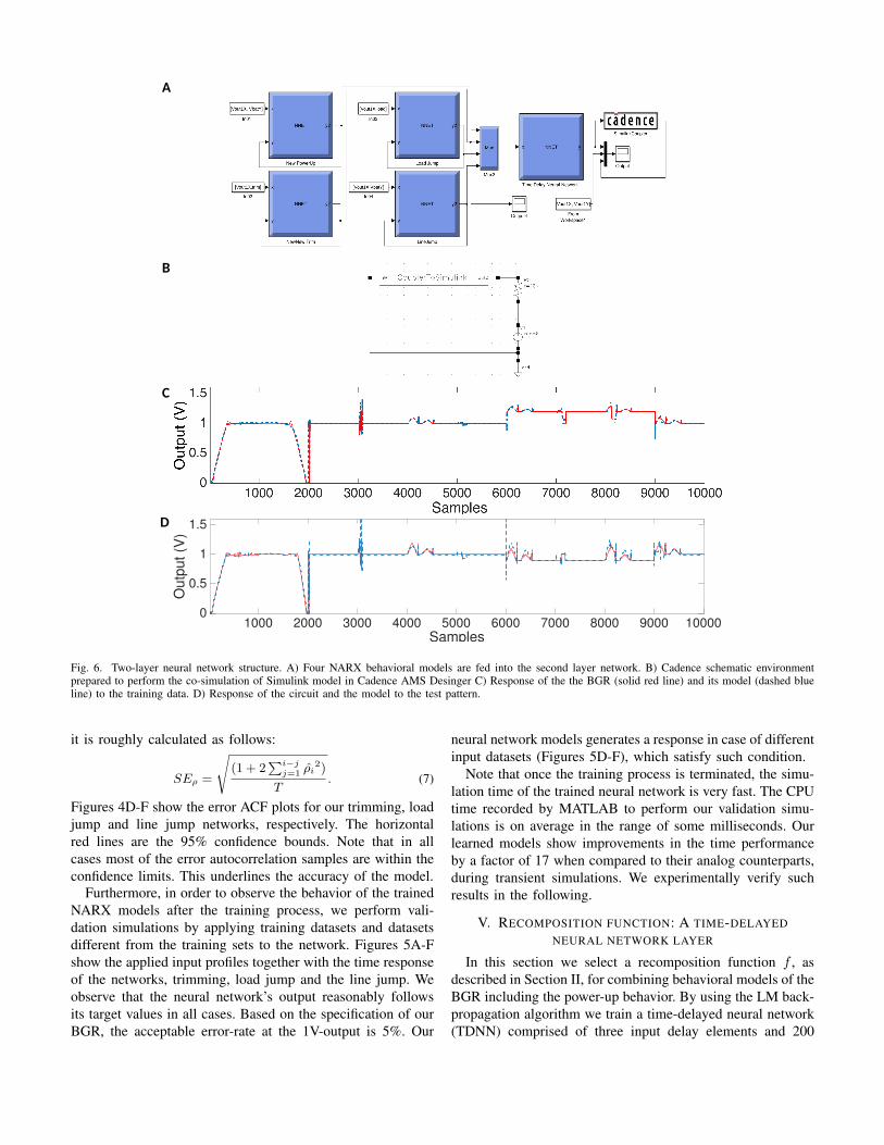
Fig. 6. Two-layer neural network structure. A) Four NARX behavioral models are fed into the second layer network. B) Cadence schematic environmentprepared to perform the co-simulation of Simulink model in Cadence AMS Desinger C) Response of the the BGR (solid red line) and its model (dashed blueline) to the training data. D) Response of the circuit and the model to the test pattern.

it is roughly calculated as follows:

SEρ =

√(1 + 2

∑i−jj=1 ρi

2)

T. (7)

Figures 4D-F show the error ACF plots for our trimming, loadjump and line jump networks, respectively. The horizontalred lines are the 95% confidence bounds. Note that in allcases most of the error autocorrelation samples are within theconfidence limits. This underlines the accuracy of the model.

Furthermore, in order to observe the behavior of the trainedNARX models after the training process, we perform vali-dation simulations by applying training datasets and datasetsdifferent from the training sets to the network. Figures 5A-Fshow the applied input profiles together with the time responseof the networks, trimming, load jump and the line jump. Weobserve that the neural network’s output reasonably followsits target values in all cases. Based on the specification of ourBGR, the acceptable error-rate at the 1V-output is 5%. Our

neural network models generates a response in case of differentinput datasets (Figures 5D-F), which satisfy such condition.

Note that once the training process is terminated, the simu-lation time of the trained neural network is very fast. The CPUtime recorded by MATLAB to perform our validation simu-lations is on average in the range of some milliseconds. Ourlearned models show improvements in the time performanceby a factor of 17 when compared to their analog counterparts,during transient simulations. We experimentally verify suchresults in the following.

V. RECOMPOSITION FUNCTION: A TIME-DELAYEDNEURAL NETWORK LAYER

In this section we select a recomposition function f , asdescribed in Section II, for combining behavioral models of theBGR including the power-up behavior. By using the LM back-propagation algorithm we train a time-delayed neural network(TDNN) comprised of three input delay elements and 200

hidden-layer neurons, to be able to take the generated output ofthe four pre-trained NARX models and to predict the correct1V-output pin of the BGR. The structure is selected with thesame approach as that of NARX models. Figure 6A representsthe structure of the two-layer network. The network responseto the training and test dataset is shown in Figure 6B and 6C,respectively. Matlab CPU time for executing the simulation ofthe network is approximately 50ms.

VI. CO-SIMULATION OF MATLAB/SIMULINK MODELS ANDANALOG DESIGN ENVIRONMENT

Here we utilize the Cadence AMS Designer/MATLAB co-simulation interface in order to evaluate the performance ofthe designed neural network model within the Analog DesignEnvironment (ADE) of Cadence software, where we executeanalog IC’s fault simulations [8]. Inside the co-simulationplatform, a coupling module is provided in order to linkSimulink and Cadence schematics environments. Figure 6Aand 6B show the simulation environments in Simulink andCadence schematics respectively. We apply inputs to the neuralnetwork block in Simulink and simultaneously run a transientsimulation in the Cadence ADE. Figure 6C and 6D depict theresults of the co-simulation in case of training input datasetand test input dataset, correspondingly. The total CPU timefor such transient simulations is calculated as 1.07s while thesame simulation of the transistor-level BGR takes 17.8s to becompleted. As a results, we gain a simulation speed-up by afactor of 17.

VII. CONCLUSIONS

We employed a new neural network modeling approach forcomplex MIMO systems (CompNN). We modeled individualI/O behavioral functions of the system by training NARX neu-ral networks. We then merged the overall behavioral featuresby training a second layer TDNN. CompNN enabled us todefine a one-to-one mapping from specific behavioral featuresof the system to certain parts of the model. We illustratedthe performance of our modeling approach by designingbehavioral NN models for a CMOS band-gap voltage referencecircuit. Individual, small-sized NARX networks were designedand trained to imitate the trimming, load jump and line jumpresponses of the BGR. Such pre-trained networks together withthe power-up behavior, were fed into a second time-delayednetwork in order to generate a single block representing theBGR.

The performance of the instructed networks were quali-tatively and quantitatively analyzed by carrying out linearregression analysis, computing the error auto-correlation func-tion and calculating the error histogram for each model. Weconfirmed the level of generalization and the accuracy ofsuch predictive neural networks by illustrating the outputresponse of the models to various input patterns differentfrom the training patterns. We subsequently created a singleneural network block by adding the second layer for mergingthe behavioral features and training the network. Finally weemployed the designed network in a transient simulation and

achieved sensible enhancement in the time performance of thesimulation.

For future work, we intend to exploit our NARX modelsin the verification of analog integrated circuits, where theinstantaneous response of the network together with its highlevel of accuracy results in significant improvements in theperformance of the pre-silicon analog fault simulations.

ACKNOWLEDGMENTS

We would like to thank Infineon for training, mentoringand provision of the tool landscape. This work was jointlyfunded by the Austrian Research Promotion Agency (FFG,Project No. 854247) and the Carinthian Economic PromotionFund (KWF, contract KWF-1521/28101/40388). Part of thisresearch work was carried out while the first author wasvisiting Imperial College London in 2016.

REFERENCES

[1] R. Narayanan, N. Abbasi, M. Zaki, G. Al Sammane, and S. Tahar,“On the simulation performance of contemporary ams hardware descrip-tion languages,” in 2008 International Conference on Microelectronics.IEEE, 2008, pp. 361–364.

[2] M. Shokrolah-Shirazi and S. G. Miremadi, “Fpga-based fault injectioninto synthesizable verilog hdl models,” in Secure System Integrationand Reliability Improvement, 2008. SSIRI’08. Second InternationalConference on. IEEE, 2008, pp. 143–149.

[3] F. Pecheux, C. Lallement, and A. Vachoux, “Vhdl-ams and verilog-amsas alternative hardware description languages for efficient modeling ofmultidiscipline systems,” IEEE transactions on Computer-Aided designof integrated Circuits and Systems, vol. 24, no. 2, pp. 204–225, 2005.

[4] W. Zhao and Y. Cao, “New generation of predictive technology modelfor sub-45 nm early design exploration,” IEEE Transactions on ElectronDevices, vol. 53, no. 11, pp. 2816–2823, 2006.

[5] S. Balasubramanian and P. Hardee, “Solutions for mixed-signal socverification using real number models,” Cadence Design Systems, 2013.

[6] M. Magerl, C. Stockreiter, O. Eisenberger, R. Minixhofer, and A. Baric,“Building interchangeable black-box models of integrated circuits foremc simulations,” in Electromagnetic Compatibility of Integrated Cir-cuits (EMC Compo), 2015 10th International Workshop on the. IEEE,2015, pp. 258–263.

[7] R. M. Hasani, D. Haerle, and R. Grosu, “Efficient modeling of complexanalog integrated circuits using neural networks,” in 2016 12th Confer-ence on Ph. D. Research in Microelectronics and Electronics (PRIME).IEEE, 2016, pp. 1–4.

[8] Cadence. Cadence Virtuoso AMS Designer Simulator, cosimulation ofmixed-signal systems with matlab and simulink. [Online]. Available:http://www.mathworks.com/products/

[9] H. T. Siegelmann, B. G. Horne, and C. L. Giles, “Computationalcapabilities of recurrent narx neural networks,” IEEE Transactions onSystems, Man, and Cybernetics, Part B (Cybernetics), vol. 27, no. 2, pp.208–215, 1997.

[10] S. A. Billings, Nonlinear system identification: NARMAX methods inthe time, frequency, and spatio-temporal domains. John Wiley & Sons,2013.

[11] J. Heaton, Introduction to neural networks with Java. Heaton Research,Inc., 2008.

[12] C.-W. Hsu, C.-C. Chang, C.-J. Lin et al., “A practical guide to supportvector classification,” 2003.

[13] H. Demuth, M. Beale, and M. Hagan, “Neural network toolbox 8.4,”Users guide, 2015.

[14] D. W. Marquardt, “An algorithm for least-squares estimation of non-linear parameters,” Journal of the society for Industrial and AppliedMathematics, vol. 11, no. 2, pp. 431–441, 1963.

[15] M. T. Hagan and M. B. Menhaj, “Training feedforward networks withthe marquardt algorithm,” IEEE transactions on Neural Networks, vol. 5,no. 6, pp. 989–993, 1994.

[16] G. E. Box, G. M. Jenkins, G. C. Reinsel, and G. M. Ljung, Time seriesanalysis: forecasting and control. John Wiley & Sons, 2015.