C.A. Munoz and J. A. Perez (Eds.) :Developments in Computational ModelsEPTCS 204, 2016, pp. 19–30, doi:10.4204/EPTCS.204.3

c© P. SobocinskiThis work is licensed under theCreative Commons Attribution License.

Compositional model checking of concurrent systems, withPetri nets

Paweł SobocinskiECS, University of Southampton, UK

Compositionality and process equivalence are both standard concepts of process algebra. Composi-tionality means that the behaviour of a compound system relies only on the behaviour of its compo-nents, i.e. there is no emergent behaviour. Process equivalence means that the explicit statespace ofa system takes a back seat to its interaction patterns: the information that an environment can obtainthough interaction.

Petri nets are a classical, widely used and understood, model of concurrency. Nevertheless, theyhave often been described as a non-compositional model, and tools tend to deal with monolithic,globally-specified models.

This tutorial paper concentrates on Petri Nets with Boundaries (PNB): a compositional, graphicalalgebra of 1-safe nets, and its applications to reachability checking within the tool Penrose. Thealgorithms feature the use of compositionality and process equivalence, a powerful combination thatcan be harnessed to improve the performance of checking reachability and coverability in severalcommon examples where Petri nets model realistic concurrent systems.

1 Introduction

This short paper is a tutorial on the algebra of Petri nets with boundaries (PNB) and its use as a com-positional formalism for the modelling of concurrent and distributed systems, and their compositionalverification via the tool Penrose. While compositional approaches to Petri nets have a long history—starting with Mazurkiewicz [9]—compositional reasoning has not had a significant impact in modellingapproaches and tools. Indeed, Penrose is the first automated reachability checker to harness composi-tionality; more established tools deal with the global statespace.

This article is deliberately non-technical and gives a high-level overview of the work on PNB. Thereader hungry for more detail will find it, together with pointers to the significant corpus of relatedwork, in the cited research papers. A comprehensive treatment can be found in Stephens’ recent PhDthesis [13].

The paper is divided into three sections: Section 2 is an overview of the algebra of PNB. Section 3 isdevoted to an explanation of how the algebra underpins a compositional algorithm for checking reacha-bility via the Penrose tool. In Section 4 we outline the main lines of anticipated future work. The readeris assumed to already be familiar with the basic concepts of Petri nets and their step semantics whereindependent transitions can be fired in parallel.

2 Compositional modelling: Petri nets with boundaries

Petri nets with boundaries (PNB) are a compositional algebra of Petri nets. The algebra was introducedfor 1-safe nets—where the step semantics ensures that there is at most one token on each place bydisabling the firing of those transitions that would violate this invariant—in the CONCUR 2010 paper by

20 Compositional model checking of concurrent systems, with Petri nets

the author [12]. Subsequently, it was extended by Bruni, Melgratti and Montanari for ordinary, infinite-state place/transitions nets in their CONCUR 2011 paper [4]. The theory was then consolidated andpresented together in a uniform manner in the jointly authored archival version [5].

To understand the basic idea of compositionality in the context of Petri nets with boundaries, it isinstructive to think of a Petri net as a system of actors (the places) that may participate in distributedsynchronisations (the transitions). Given a particular synchronisation, it is then possible to take a localview from the point of a subset of the involved actors. Indeed, the local information relevant to a singleactor is:

1. whether it is able to participate in the synchronisation, i.e. does it satisfy the requirements of thePetri net transition?

2. if so, what is the effect of the synchronisation on its internal state: i.e. what is the effect of firingthe transition on its number of tokens?

Let us illustrate these points on the most trivial relevant example: a 1-safe Petri net with a single transitionthat takes a token from place A and produces one at place B.

A B (1)

Here we can think of A and B as simple computational entities that can be in one of two states: 0 or 1depending on whether a token is present. In order for the synchronisation—the firing of the transitionin (1)—to occur, A must contain a token and B must be empty. The effects of the synchronisation are toremove the token from A and place a token on B.

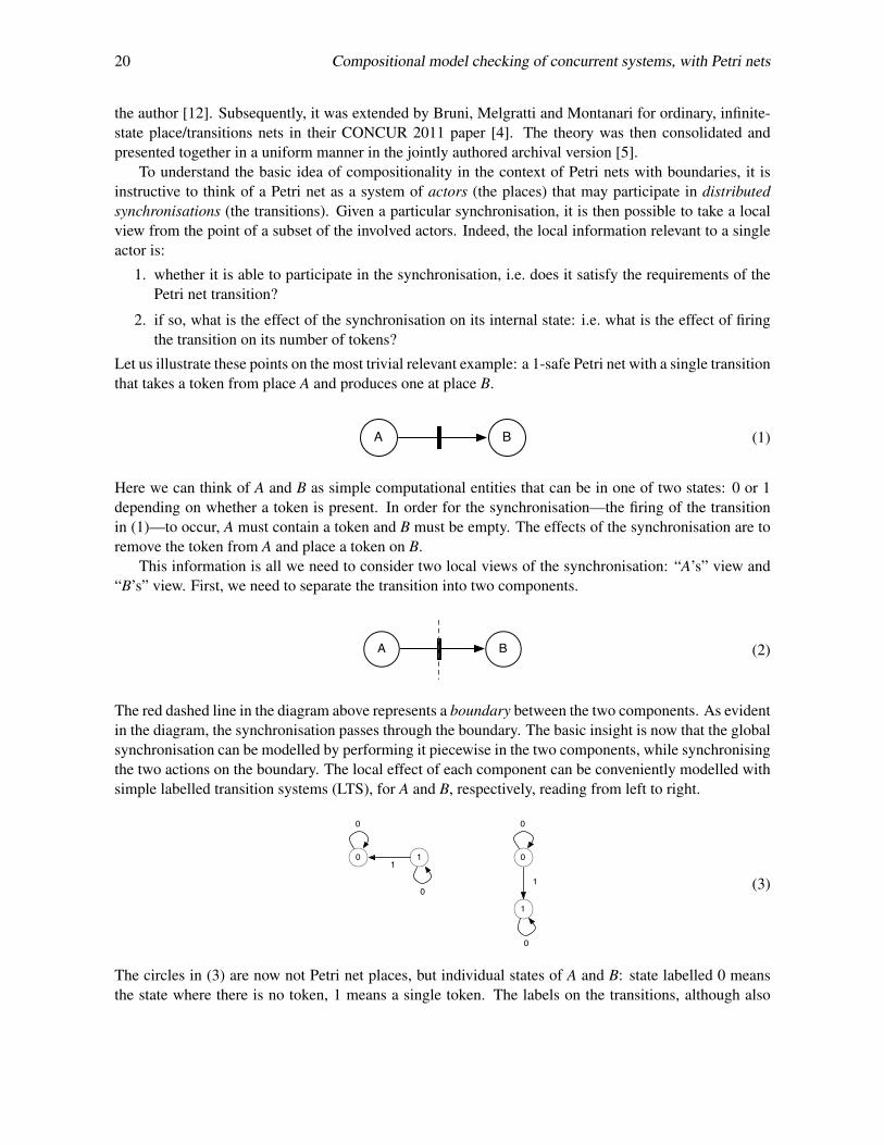
This information is all we need to consider two local views of the synchronisation: “A’s” view and“B’s” view. First, we need to separate the transition into two components.

A B (2)

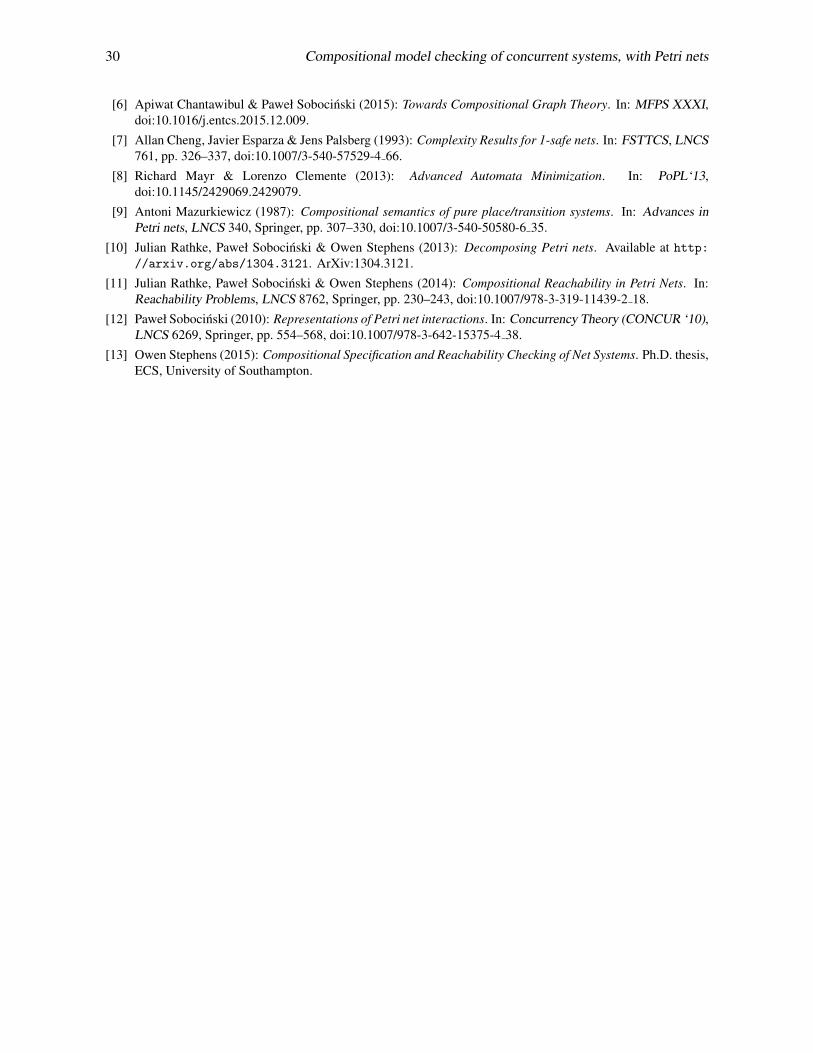
The red dashed line in the diagram above represents a boundary between the two components. As evidentin the diagram, the synchronisation passes through the boundary. The basic insight is now that the globalsynchronisation can be modelled by performing it piecewise in the two components, while synchronisingthe two actions on the boundary. The local effect of each component can be conveniently modelled withsimple labelled transition systems (LTS), for A and B, respectively, reading from left to right.

101

0

0

1

0

1

0

0

(3)

The circles in (3) are now not Petri net places, but individual states of A and B: state labelled 0 meansthe state where there is no token, 1 means a single token. The labels on the transitions, although also

P. Sobocinski 21

labelled with 0s and 1s, refer to something quite different: the capability of changing the internal stateof the component, while possibly engaging in synchronisation. Whether or not a state transition engagesin a synchronisation is represented by the label of the transition, and can be thought of as what can beobserved on the boundary.

The label 0 means that no synchronisation is engaged. As witnessed by the loop transitions on eachstate, each component, in each state, has the possibility of not changing state by not engaging in anytransitions. Indeed, the transition systems that arise from PNB are always reflexive in this sense: everyLTS state has a self-looping 0 labelled transition. The label 1 means that the synchronisation has beenengaged in exactly once. For example, in the left transition system of (3) that corresponds to place A, the1 labelled transition records the fact that when the transition fires the place loses its token: that is, thereis a transition from state 1 to state 0.

In the 1-safe case, there can be no auto-concurrency on transitions and thus the LTS transition alpha-bet is limited to the set {0,1}. In the infinite state case, however, it is natural to consider the labels comingfrom the set of the natural numbers, since individual transitions can, in principle be fired simultaneously:see [5] for the details.

Now to obtain the global step semantics of the original Petri net (1) one needs to synchronise the twotransition systems. The synchronisation is a natural variant of the cartesian product of the two transitionsystems: the resulting states are simply ordered pairs of states of the original LTSs, and a transition(a,b)→ (a′,b′) exists whenever we can find a α−→ a′ and b α−→ b′ in the original transition systems. Thefact that α is the same label in both component transitions means that we are synchronising the two onthe common boundary.

0,0 1,0

0,1 1,1

The above transition system represents the result of the synchronisation: we see that, as expected, theonly non-trivial behaviour of the net (1) is when place A contains one token and place B zero tokens: inthat case, the transition can be fired, resulting in a transition to the state where the token placement hasbeen inverted.

The basic ideas outlined above can be distilled into two observations:

1. net transitions, seen as a distributed synchronisations, can be separated into individual components;

2. the seemingly fundamental classification of inputs and outputs of a particular net transition isactually local — whether a synchronisation acts as an input (token consumer) or an output (tokenproducer) is something that is determined by the individual component’s transition system.

These observations leads to the notion of algebra of components, which consists of two operationsthat allow us to connect them into composite, interacting networks. They also suggest an alternativegraphical notation that makes the input/output assignment of transition endpoints local; it is the graph-ical syntax adopted in the literature on PNBs and we will use it henceforward. The net (1), using the

22 Compositional model checking of concurrent systems, with Petri nets

alternative graphical syntax, is pictured below.

A B (4)

Each place now has two ports: an input port, drawn as a black triangle pointing into it, and an outputport, represented by the black triangle pointing out. A transition is determined by a subset of the set ofall ports of a particular net: in (4) the transition is the set containing the output port of A and the inputport of B. The vertical line through the transition is a notational convenience that helps to distinguishbetween different transitions.

Roughly speaking, rather than directing transitions, we direct the places. It is not difficult that thetwo graphical representations have equal expressive power and we can readily translate between them.The alternative graphical syntax comes into its own when describing net components, because it freesone from the red-herring distraction of directed transitions and the implicit type information it brings:for example, it is no problem to, for instance, connect an “input to an input”: the result is that two partialviews of a synchronisation are combined, and the two local input actions are synchronised.

The intuitive idea of separating the simple synchronisation (2) into its constituents has a formal statusas a PNB expression (6). Its two components are illustrated below.

A B (5)

Here the common boundary is made explicit: it is represented by the boundary ports: one on the righthand side of the box that encloses the place A and the second the left hand side of the box around placeB. A boundary port plays a similar role to the input and output ports on places in the sense that transitioncan connect to them: here the original transition connecting A and B has been split into a transition thatconnects the output port of A with the right boundary port in the first component, and a transition thatconnects the input port of B with the left boundary port in the second. Note that, although ports canappear either on the left or on the right, they ought not be confused with inputs and outputs since theyact merely as synchronisation points; as previously mentioned, inputs and outputs are notions local toplaces. Indeed, one could just as well use the components below in a decomposition of (4); intuitively,now, the flow is from right to left.

;

In terms of a physical intuition, the boundary ports play a role akin to terminals in engineering terminol-ogy; the idea is that a system interacts with its environment via its terminals.

There are two operations with which one can compose PNB components. The first is compositionalong a common boundary. Given a PNB M of type (m,k), where m,k ∈ N are the numbers of, respec-tively, the left hand side ports and the right hand side ports, and a PNB N of type (k,n), we obtain a PNBM ; N of type (m,n). The places of M ; N are the disjoint union of the places of M and N; its transitions

P. Sobocinski 23

are the union of the transitions of M and N which do not connect to the common boundary, together withsynchronisations of those transitions that do connect to boundary ports. For example, composing the twocomponents in (5) of type (0,1) and (1,0), respectively, yields the PNB of type (0,0) illustrated below.

A B =; A Bqp

{p,q}(6)

The transition {p,q} in the result is the synchronisation of p and q in the constituent components. Ratherthan dwell on the formal details of the definition of composition, which can be found in [5], we illustrateit with a number of examples which give the intuition.

t

u

a

b

{t,a}

{u,b}

t

u

c

d

e{u,e}

{t,c}

{t,d}

t

u

f {t,f}t

ug {t,g,u}

P : (0,2) Q : (2,0) P ; Q : (0,0) P : (0,2) R : (2,0) P ; R : (0,0)

P : (0,2) S : (0,2) P ; S : (0,0) P : (0,2) T : (0,2) P ; T : (0,0)

Starting with the top left example, we see that a composite net is obtained by synchronising transitionson two separate ports. Note that the order of the ports is significant. The top right example contains twointeresting situations: first, the two transitions c and d of component R both connect to the upper left handside port. In the composition, transition t can synchronise with either and both the possibilities, {t,c}and {t,d} are transitions in the resulting net. The synchronisation on the second port is also of interest:here e is a transition that connects only to the port. The result of synchronising u with e is that u iscompleted; and becomes a transition which does not have any effect on the places coming from the rightcomponent. While seemingly spurious, transitions that connect only to boundary ports are actually veryuseful in examples, as we will see in Section 3. In the lower left example, we see that the composition hasthe effect of synchronising all three of the transitions t, u and g, even though t and u were not originallysynchronised. This is because the transition g is connected to both of the boundary ports: thus, to forma part of a transition in the result it needs to synchronise with corresponding transitions that connect tothe shared boundary ports in the left hand side component. Finally, the lower right example ought to becontrasted with the upper right: here there is a single transition f that connects to the upper left boundaryport and the two places. The result in the composition is a single synchronisation {t, f}. On the otherhand, u now has no partner transition in T with which it can synchronise, therefore there is no transitionin the composition that has u as a component.

The second operation of the algebra of PNB is a non-interacting parallel composition. Given nets Mof type (m1,n1) and N of type (m2,n2), their parallel composition M⊕N has type (m1 +m2,n1 + n2).

24 Compositional model checking of concurrent systems, with Petri nets

This operation is much easier to describe: the resulting net is simply the disjoint union of the two nets,where the left and right ports of M come before (ordering from top to bottom) the respective ports of N.Graphically, this can be understood simply as “stacking” M on top of N. This operation is very usefulin constructing cyclic networks (e.g. a token ring) as well as nets with repeated structure, such as trees,see [10, 13] for examples. The simplicity of the examples in this tutorial means that we will not need touse it further.

The passage from a net component to its transition system, as previewed in the move from (2) to (3)gives us a notion of semantics of PNB. The semantics is a two-labelled transition system (2LTS); eachtransition has two labels. For instance, let us focus the semantics of the PNB pictured below.

(7)

Its transition system, pictured below, has as its states the possible markings of the net; in the particularcase of (7) there are just two possible markings, so two states.

0

1

1/00/1

0/0

0/0

(8)

As mentioned previously, each transition of (8) has two labels: the first to the left of the ‘/’ separator andthe second to the right. The left label refers to the interactions on the left boundary, and similarly, theright to the interactions on the right. In particular, at the empty marking (state 0), the net can synchroniseon the left, producing a token, that is transitioning to state 1. From that state, it can synchronise onthe right to come back to the empty marking. In any state there is the option of not synchronising andremaining in the same state. In general, the left and right labels are words over the alphabet {0,1}, theirlength determined by the size of the boundary. Specifically, a net M of type (m,n) will have all of itstransitions having labels of the form α/β where α ∈ {0,1}m and β ∈ {0,1}n. The general procedure ofobtaining a 2LTS from a PNB can be seen as a straightforward generalisation of the familiar notion ofstep firing semantics.

There is also a straightforward way of defining the operations of ; and ⊕ directly on 2LTS, and bothare variants of the product of transition systems. For example, the rule

aα/β−−→ a′ b

β/γ−−→ b′

(a,b)α/γ−−→ (a′,b′)

(9)

defines the composition ‘;’ and witnesses our intuition of this operation as synchronisation along a sharedboundary.

Compositionality of the formalism can now be expressed precisely: given nets M of type (m,k) andN of type (k,n), to obtain the semantics of M ; N we can either

P. Sobocinski 25

• translate M and N individually into transition systems and compose them using (9);

• compose M and N as PNBs and obtain a transition system for the composite net, using the stepfiring semantics.

Compositionality means that it does not matter which choice is made: the two transition systems areguaranteed to be isomorphic.

We conclude this section with a brief observation on the category theoretic account of composi-tionality, in the sense described above. Petri nets with boundaries form the arrows of a prop: a strictsymmetric monoidal category with object the natural numbers, where the monoidal product on objectsis addition. Next, two-labelled transition systems are also the arrows of a prop. Then compositionality,stated succinctly, is that the translation from nets to transition system is a prop homomorphism.

3 Compositional reachability checking

Our running example for this section is a simple, modular specification of a counter Petri net1 using thealgebra of PNB. An n-bit counter consists of n basic components, each modelling the behaviour of anindividual bit. The component that models the behaviour of each bit is illustrated below.

0

1

inccarry

Assuming a token on place zero, a synchronisation on the right boundary port (marked inc) flips the bitto 1, that is, the token is removed from place 0 and placed at 1. Another synchronisation on port inc,enabled when there is a token at place 1, takes us to the starting state, but the synchronisation now alsoinvolves the left hand side carry port, which in turn affects the state of higher order bits. For example,composing three of these components in series gives us a 3-bit counter, as illustrated below. In thegraphical representation of the result of the composition, colours and various line styles have been usedin order to help distinguish between the transitions.

0

1

0

1

0

1

0

1

0

1

0

1=; ; ; ;

(10)One natural question to ask about the n-bit counter net in general is whether the state in which all of thebits are 1 is reachable from the state in which they are all in state 0. Traditionally, algorithms for decidingreachability consider the global state space, but in our counter example, the shortest firing sequence fromthe initial state to the desired state has length 2n−1. This is not surprising; indeed, reachability checkingfor safe nets is PSPACE-complete [7].

1This example was prompted by a question by Moshe Vardi during the DCM workshop in Cali, Colombia, in October 2015.

26 Compositional model checking of concurrent systems, with Petri nets

Here the compositional approach can be useful. First, note that the reachability question itself is in-herently local in the sense that the reachability problem leads us to consider each component’s transitionsystem as a nondeterministic finite automaton (NFA): the starting state being the initial marking and thefinal state(s) the desired marking(s). This idea is illustrated below: starting with the transition systemfor a counter net component, illustrated on the left, we can associate the reachability specification andconsider it as an automaton. Indeed, the initial state is when the bit is in state 0, and the final state 1 isthe desired marking.

0

1

0/11/1

0/0

0/0

0

1

0/11/1

0/0

0/0

1

(11)

Clearly, the reachability question of the n-bit counter net reduces to language emptiness of the composed,global automaton that is the semantics of the composed net. This automaton has 2n states, so by itself,it is not very useful. Here compositionality combined with language equivalence does the trick. Toillustrate this point, let us consider the following composition, the rightmost part of (10).

0

1;

0

1= (12)

Using compositionality, the automaton for (10) can be obtained by composing (11) with the automaton

?

0/ε

1/ε

(13)

which is the semantics of the rightmost component in the composition (10). The result is the following:

0,∅

1,∅

0/ε

1,∅

1/ε

0/ε

0/ε

(14)

At this point, it is instructive to take a step back and discuss further the role of the zero transitions. Byzero transitions we mean those where the component labels are strings made up solely of 0s. We haveseen, starting with (3) that the transition systems that underlie PNB components are reflexive: at each

P. Sobocinski 27

state there is a looping zero transition. But not all zero transitions are self loops; for example, in thetransition system of (14), there is 0/ε transition from state (0,∅) to state (1,∅); it corresponds to thefiring of an internal transition—that is, one not connected to a boundary port—of the component that isthe result of the composition in (12).

The fact that zero transitions are internal means that they can be safely ignored when reasoning aboutthe behaviour of composed nets. More precisely, weak language equivalence is a congruence wrt to theoperations (⊕ and ;) of PNBs [11, Proposition 8]. Weak language equivalence is closely related to theclassical notion of ε-closure in NFAs; zero transitions are treated akin to ε-transitions. This means thatwe can replace (14) with any (smaller) weak language equivalent automaton and use it in subsequentcompositions, without sacrificing correctness wrt reachability checking. Indeed, the automaton (14) canbe replaced with the weakly equivalent (13).

At this point, we have a proof of reachability since adding additional counter components will resultin (13). This procedure has been automated, resulting in the tool Penrose, as detailed in [11, 13]. Theinput to the tool is a PNB expression, such as (10), viewed as a syntax tree where the leaves are labelledby individual PNB, and the internal nodes by the PNB operations ⊕ and ;. The computation done by thetool can then be summarised as consisting of the following steps:

(i) Translate the leaves of the expression to automata, then evaluate, bottom up, as follows.

(ii) In order to compose automata A and B, first minimise them wrt weak language equivalence, obtain-ing A′ and B′, then compose, and minimise again. For minimisation, Penrose adapts algorithmsrecently proposed by Mayr and Clemente in [8], which does not guarantee optimality but is quiteefficient in practice.

(iii) At each point, check for language emptiness; if at any point the language is empty then answer NO(not reachable). In the final step (corresponding to the root of the expression), non-emptiness isequivalent to reachability.

In order to understand the algorithm, it is useful to run through a particular example execution. Forthe 3-bit counter, the input is the expression

0

1

;

;

0

1

;

0

1

;

(15)

together with the information that we want to check the reachability of state 111 from state 000. Given

28 Compositional model checking of concurrent systems, with Petri nets

this, we can transform the leaves to automata.

;

;

;

;

0

1

0/11/1

0/0

0/0

1

0

1

0/11/1

0/0

0/0

1

0

1

0/11/1

0/0

0/0

1

?

0/ε

1/ε

?

ε/0

ε/1

Performing the first, deepest composition and minimisation, as explained previously, yields

;

;

;

0

1

0/11/1

0/0

0/0

1

0

1

0/11/1

0/0

0/0

1 ?

0/ε

1/ε

?

ε/0

ε/1

At this point Penrose uses memoisation to avoid doing the same (up-to language equivalence on thearguments) composition repeatedly. We use the recent advances in NFA language equivalence checkingby Bonchi and Pous [1] to make this procedure efficient. At the final step we arrive at the triviallyaccepting automaton

?

ε/ε

thereby verifying the reachability of 111 from 000. The combination of compositionality and weaklanguage equivalence means that our problem, in which the execution path from the initial state to thefinal state is exponential in the size of the net, can be solved algorithmically in linear time.

P. Sobocinski 29

The sceptical reader will no doubt wonder if this carefully chosen example is indicative of the utilityof the technique in more realistic, practical examples. We have performed a compositional analysis on astandard set of benchmark examples. In several of these Penrose, unsurprisingly, beats its competitorswhich do not have access and do not take advantage of the high-level component-wise specification.See [11, 13] for a detailed account of the experimental results. In fact, many (most?) practical systemsare quite modular by design, and thus consist of networks of repeated components: for many of suchsystems Penrose does very well, in several cases outperforming other tools by factors of magnitude.

4 Future work

In recent years, the Bonchi, Zanasi and the author have studied the algebraic theory of signal flow graphsusing props, see e.g. [2, 3]. The algebraic theory of PNB can be studied using similar techniques, butthe picture is both more interesting and more complex because one can study theories wrt a processequivalence such as language equivalence or bisimilarity. Even merely sound theories could be useful formodel checking, since components could in principle be simplified as nets before translating to automata.

Next, the algorithm presented in Section 3 could be extended to deal with parametric examples: e.g.instead of asking for the reachability in a 23-bit counter, one could ask the question in more generalityfor an n-bit counter, where the n is a formal parameter. To achieve this, Penrose could be extendedwith logic that detects fixed points, such as the one encountered when evaluating the counter example—clearly, after the first composition and minimisation step, reachability has been decided for counters ofarbitrary size. There are challenging related problems, including investigating heuristics and strategiesfor obtaining fixed points during evaluation.

A related, very challenging problem, and one that is currently completely side-stepped by Penrose,is obtaining efficient decompositions, that is expressions such as (15), which are currently provided asinput. Ideally, the process of finding the decomposition itself ought to be automated. Here there areconnections with graph theory, and in particular the notion of rank-width; some initial work has beendone in [10] and the connection with graph theory was made explicit in [6].

Finally, one could use the algebra of infinite state case PNBs to obtain approximations to reachability(and coverability) for infinite state nets; a decidable problem that it notoriously challenging for boththeory and tool development.

References

[1] Filippo Bonchi & Damien Pous (2013): Checking NFA Equivalence with Bisimulations up to Congruences.In: PoPL‘13, doi:10.1145/2429069.2429124.

[2] Filippo Bonchi, Paweł Sobocinski & Fabio Zanasi (2014): A Categorical Semantics of Signal Flow Graphs.In: CONCUR‘14, LNCS 8704, Springer, pp. 435–450, doi:10.1007/978-3-662-44584-6 30.

[3] Filippo Bonchi, Paweł Sobocinski & Fabio Zanasi (2015): Full Abstraction for Signal Flow Graphs. In:Principles of Programming Languages, POPL‘15., doi:10.1145/2676726.2676993.

[4] Roberto Bruni, Hernan C. Melgratti & Ugo Montanari (2011): A Connector Algebra for P/T Nets Interac-tions. In: Concurrency Theory (CONCUR ‘11), LNCS 6901, Springer, pp. 312–326, doi:10.1007/978-3-642-23217-6 21.

[5] Roberto Bruni, Hernan C. Melgratti, Ugo Montanari & Paweł Sobocinski (2013): Connector Algebras forC/E and P/T Nets’ Interactions. Log. Meth. Comput. Sci. 9(3), doi:10.2168/LMCS-9(3:16)2013.

30 Compositional model checking of concurrent systems, with Petri nets

[6] Apiwat Chantawibul & Paweł Sobocinski (2015): Towards Compositional Graph Theory. In: MFPS XXXI,doi:10.1016/j.entcs.2015.12.009.

[7] Allan Cheng, Javier Esparza & Jens Palsberg (1993): Complexity Results for 1-safe nets. In: FSTTCS, LNCS761, pp. 326–337, doi:10.1007/3-540-57529-4 66.

[8] Richard Mayr & Lorenzo Clemente (2013): Advanced Automata Minimization. In: PoPL‘13,doi:10.1145/2429069.2429079.

[9] Antoni Mazurkiewicz (1987): Compositional semantics of pure place/transition systems. In: Advances inPetri nets, LNCS 340, Springer, pp. 307–330, doi:10.1007/3-540-50580-6 35.

[10] Julian Rathke, Paweł Sobocinski & Owen Stephens (2013): Decomposing Petri nets. Available at http://arxiv.org/abs/1304.3121. ArXiv:1304.3121.

[11] Julian Rathke, Paweł Sobocinski & Owen Stephens (2014): Compositional Reachability in Petri Nets. In:Reachability Problems, LNCS 8762, Springer, pp. 230–243, doi:10.1007/978-3-319-11439-2 18.

[12] Paweł Sobocinski (2010): Representations of Petri net interactions. In: Concurrency Theory (CONCUR ‘10),LNCS 6269, Springer, pp. 554–568, doi:10.1007/978-3-642-15375-4 38.

[13] Owen Stephens (2015): Compositional Specification and Reachability Checking of Net Systems. Ph.D. thesis,ECS, University of Southampton.