Compositional Analysis of Habitat Use From Animal … · COMPOSITIONAL ANALYSIS OF HABITAT USE FROM ... Fordingbridge, Hampshire SP6 JEF United Kingdom ... Jennrich and Turner 1969;

Compositional Analysis of Habitat Use From Animal Radio-Tracking DataAuthor(s): Nicholas J. Aebischer, Peter A. Robertson, Robert E. KenwardSource: Ecology, Vol. 74, No. 5 (Jul., 1993), pp. 1313-1325Published by: Ecological Society of AmericaStable URL: http://www.jstor.org/stable/1940062Accessed: 20/05/2010 12:48

Your use of the JSTOR archive indicates your acceptance of JSTOR's Terms and Conditions of Use, available athttp://dv1litvip.jstor.org/page/info/about/policies/terms.jsp. JSTOR's Terms and Conditions of Use provides, in part, that unlessyou have obtained prior permission, you may not download an entire issue of a journal or multiple copies of articles, and youmay use content in the JSTOR archive only for your personal, non-commercial use.

Please contact the publisher regarding any further use of this work. Publisher contact information may be obtained athttp://www.jstor.org/action/showPublisher?publisherCode=esa.

Each copy of any part of a JSTOR transmission must contain the same copyright notice that appears on the screen or printedpage of such transmission.

JSTOR is a not-for-profit service that helps scholars, researchers, and students discover, use, and build upon a wide range ofcontent in a trusted digital archive. We use information technology and tools to increase productivity and facilitate new formsof scholarship. For more information about JSTOR, please contact [email protected].

Ecological Society of America is collaborating with JSTOR to digitize, preserve and extend access to Ecology.

http://dv1litvip.jstor.org

http://www.jstor.org/stable/1940062?origin=JSTOR-pdf

http://dv1litvip.jstor.org/page/info/about/policies/terms.jsp

http://www.jstor.org/action/showPublisher?publisherCode=esa

Ecology, 74(5), 1993, pp. 1313-1325 Cc 1993 by the Ecological Society of Amenica

COMPOSITIONAL ANALYSIS OF HABITAT USE FROM ANIMAL RADIO-TRACKING DATA'

NICHOLAS J. AEBISCHER AND PETER A. ROBERTSON The Game Conservancy, Fordingbridge, Hampshire SP6 JEF United Kingdom

ROBERT E. KENWARD Institute of Terrestrial Ecology, Furzebrook Research Station,

Wareham, Dorset BH20 SAS United Kingdom

Abstract. Analysis of habitat use based on radio-tagged animals presents difficulties inadequately addressed by current methods. Areas of concern are sampling level, data pooling across individuals, non-independence of habitat proportions, differential habitat use by groups of animals, and arbitrary definition of habitat availability. We advocate proportional habitat use by individual animals as a basis for analysis. Hypothesis testing of such nonstandard multivariate data is done by compositional analysis, which encom- passes all MANOVA/MANCOVA-type linear models. The applications to habitat use range from testing for age class effects or seasonal differences, to examining relationships with food abundance or home range size. We take as an example the comparison of habitat use and availability. The concepts are explained and demonstrated on two data sets, illustrating different methods of treating missing values. We compare utilized with available habitats in two stages, examining home range selection within the overall study area first, then habitat use within the home range. At each stage, assuming that use differs from random, habitats can be ranked according to relative use, and significant between-rank differences located. Compositional analysis is also suited to the analysis of time budgets or diets.

Key words. compositional analysis, gray squirrel, habitat use; radiotelemetrv, Ring-necked Pheas- ant; time-budget analysis.

INTRODUCTION

Many studies of habitat use by wild animals use radio tracking as a source of data. Common aims are to determine whether a species uses habitats available to it at random, to rank habitats in order of relative use, to compare use by different groups of animals, e.g., males and females, to relate use to variables such as temperature and food abundance, or to examine the effects of habitat on movement and home range size. Recent reviews describe the techniques currently available (White and Garrott 1990) and compare their efficiency under a range of conditions (Alldredge and Ratti 1986, 1992). However, all available techniques contain at least one of four shortcomings affecting the validity of the analysis, often at the statistical level. The problems are detailed below, with proposed ways of overcoming them. For statistical treatment, we recommend methods based on the log-ratio analysis of compositions (Aitchison 1986).

PROBLEMS IN ANALYZING DATA ON

HABITAT UTILIZATION

Problem 1. Inappropriate level of sampling and sample size

Many analyses take the radio location as the sample unit, and the number of radio locations, often pooled

I Manuscript received 17 October 1991; revised 25 Sep- tember 1992; accepted 26 September 1992.

over several individuals, as the sample size (e.g., Smith et al. 1982, Byers et al. 1984). This can lead to two separate forms of non-independence. First, the posi- tions of sequentially collected radio locations from a tagged animal may be serially correlated (Swihart and Slade 1 985a). Second, animals usually show individual variation in behavior; pooling data across animals is justifiable only if they do not differ. Either situation inflates the apparent number of degrees of freedom, rendering statistical tests over-sensitive (increase in Type I error).

In fact, radio locations represent a subsample of an animal's behavior pattern. As in a mixed-model nested ANOVA, hypotheses concerning the population of animals must be tested at the animal level (e.g., Sokal and Rohlf 1981). The problems above disappear when the animal rather than the radio location is taken as the sample unit (Kenward 1992). An animal's habitat use is estimated either by the proportion of radio locations within each habitat or by the proportion of home range area (evaluated from the radio locations) occupied by each habitat.

Problem 2. Non-independence of proportions

The proportions that describe habitat composition sum to 1 over all habitat types (unit-sum constraint). An animal's proportional use of one habitat type is linked to that of other habitat types, thereby invali- dating the use of the Friedman (1 937) and Quade ( 1979)

1314 NICHOLAS J. AEBISCHER ET AL. Ecology, Vol. 74, No. 5

tests (see Alldredge and Ratti 1986, White and Garrott 1990). A consequence of the constraint is that an animal's avoidance of one habitat type will almost in- variably lead to an apparent preference for other types, so the interpretation of absolute preference/avoidance of habitat types (Neu et al. 1974, Byers et al. 1984) is fraught with difficulty. A technique should test for overall departure from random habitat use; given nonrandom use, it should determine which habitat types are used more and which less than expected by chance, taking into account utilization of other habitats. John- son's (1980) method recognizes the unit-sum constraint and fulfils the criteria; unfortunately it does not extend to Problem 3.

Problem 3. Differential habitat use by groups of individuals

Animals within a population may fall into distinct categories, determined for instance by age or size class, sex, or region, or by combinations of these and other factors. Animals from different categories may use habitat differently. Chi-square analysis or log-linear modelling have been proposed to test for such differences (Heisey 1985, White and Garrott 1990), but both are based on numbers of radio locations and so are open to non-independence difficulties (Problem 1). They assume also that the counts of radio locations follow a multinomial or product multinomial distribution across all dimensions of the classifying table (Dobson 1983). Assessment of goodness-of-fit is simple but often ignored, despite the inappropriateness of drawing con- clusions from badly fitting statistical models. What is needed is a method analogous to ANOVA, in which the sample size is the number of animals in each group (see Problem 1) and in which between-group differences are tested by reference to within-group between- animal variation. Ideally, the method should also extend to investigating relationships between habitat use and continuous variables, such as home range area or food abundance, measured for each individual.

Problem 4. Arbitrary definition of habitat availability

Almost all methods compare habitat use with some measure of habitat availability. However, available habitat is usually defined from the total study area. Boundary selection for a study area is usually arbitrary (Johnson 1980, Porter and Church 1987). Even in the case of a discrete island population, not all the area may be available to an animal, as it may be constrained by the presence of other animals. Following animals at different sites or in different years complicates the definition of available habitat.

From a biological viewpoint, an animal's use of the available habitat may be considered the outcome of choices at different levels (Wiens 1973, Johnson 1980, Porter and Church 1987). First, the animal lives in a certain part of an arbitrarily defined study area. Second,

within the area delimited by the animal's movements, it will select for specific sub-areas. Different forms of habitat selection may occur at each level, so analyses should be carried out in stages to identify these effects.

METHODS OF DATA ANALYSIS

Rationale behind proportional habitat use

An animal's movements determine a trajectory through space and time; its habitat use is the proportion of the trajectory contained within each habitat type. Radiotelemetry data approximate the trajectory by sampling it at discrete intervals. If sampling is repre- sentative and sufficiently frequent to record little-used habitat types, then the proportion of radio locations in each habitat estimates the proportion of the trajectory in each habitat. In this case, serial correlation between radio locations is irrelevant; more frequent sampling more closely approximates the underlying trajectory, thus providing more precise estimates of proportional habitat use, even though it also increases serial correlation.

From this viewpoint, the emphasis shifts naturally from radio location to trajectory. As habitat use by a population is that of the "average" member, it should be estimated from the trajectories of a random sample of individuals from the population. The sample size is the number of tracked individuals; numbers of radio locations are relevant only in affecting the accuracy of reconstructed trajectories. The extreme case of one radio location per animal may be compensated for by increasing the number of animals (equivalent to estimating habitat use by a point count of individuals, as in Neu et al. 1974), whereas consideration of one individual yields no information about population habitat use, however numerous the radio locations.

An extension of the trajectory is the home range, or area within which an animal's trajectory is located during a given period. Current methods of extrapolating from trajectory to home range rely on the areal distribution of radio locations (Kenward 1987, White and Garrott 1990), noting that for methods that rely on intensity of use (harmonic mean: Dixon and Chapman 1980) or probability densities (bivariate normal ellipse: Jennrich and Turner 1969; kernel: Worton 1989), the estimated home range is actually the area enclosed by an isopleth of intensity/probability chosen by the re- searcher, e.g., 95%. In the context of an underlying trajectory, serial correlation is only a problem for the probabilistic methods, which assume independence between points (see Swihart and Slade 1985b). For any method, what matters is the stability of the home range estimate with increasing numbers of radio locations. The number of radio locations necessary to achieve stability may be assessed by plotting home range area against number of locations (Kenward 1982, 1987, Parish and Kruuk 1982, Harris et al. 1990). Having estimated the home range, the area within it occupied

July 1993 ANALYSIS OF HABITAT USE 1315

by each habitat type can be expressed as a proportion of the total range area.

If radio-tracked individuals are independent (e.g., not members of the same flock or herd), considering their proportional habitat use resolves Problem 1.

The unit-sum constraint and compositional analysis

Given D habitat types, an individual's proportional habitat use is described by x, x, . . ., x,, where x, is the proportion of the individual's trajectory or home range in habitat i. The unit-sum constraint is ED1l xi =

1. Equivalently, use of habitat i as measured by xi is not independent of the use of other habitats. A set of components summing to 1 is a composition; Aitchison (1986) showed that for any component x, of a composition, the log-ratio transformation yi = ln(xi/x,) (i = 1, . . ., D, i j A) renders the y, linearly independent (technically, it is a one-to-one map of a point on a D-dimensional simplex to a point in full (D - 1)-dimensional space). He called compositional analysis the application, to these log-ratios, of the range of statis tical procedures such as MANOVA based on multivariate normality (e.g., Cox and Hinkley 1974, Mor- rison 1990). Because the log-ratio transformation is equivalent to centering the ln(x,) in relation to their mean, the results of such analyses are independent of the component x, chosen as denominator in the log- ratio transformation.

Multivariate analysis of log-ratios: generalities

Many statistical models may be fitted to the transformed compositions to test appropriate hypotheses. Although the fitting process makes no distributional assumptions, standard hypothesis testing assumes multivariate normality of the residuals. We denote by Nj(M, Z) a multivariate normal distribution of dimen- sion n, mean vector A and covariance matrix M. Ait- chison (1986) describes several ways of verifying whether residuals conform to such a distribution. How- ever, if non-normality exists, multivariate normal tests may be replaced by ones based on data randomization (Manly 1991).

Multivariate regression and MANOVA models en- able many hypotheses concerning habitat use to be tested. Both involve multivariate linear models of the form Y = AO + E, where Y is a log-ratio data matrix, A a regressor matrix, 0 a parameter matrix, and E the error matrix, assumed to consist of independent row vectors each distributed as ND-I (0, Z). Estimation of 0 and M may proceed either by maximum likelihood or multivariate least squares. Hypothesis testing relies on a generalized likelihood ratio statistic A as follows. Given a general model M, with m, parameters, and a reduced model M2 with m2 < ml parameters corresponding to a specific hypothesis (constraint) on the parameters of Ml, let Ri be the residual sum-of-squares

and cross-product matrix resulting from model M, (i = 1, 2); then A = I R. I/1 R2 1. The quantity -N in A, where N is the number of rows of Y, is distributed approximately as x2(m, - m2). Exact transformations of A to an F statistic exist in some cases (see Aitchison 1986).

Simple MANOVA applications in the context of habitat use are testing for sex, age, or seasonal differences. Multivariate regression can relate changes in habitat use to one or more independent continuous variables (mass, food supply, etc.). These powerful techniques answer Problem 3.

Comparison of utilized and available habitats

Basis of a coherent preference theory. -If a habitat type is used more than expected from its availability, it is often said to be "preferred." The notion of "preference" is useful so long as it is used on a relative scale which allows habitat types to be ranked from "least preferred" to "most preferred" (absolute statements about preference are dangerous because of Problem 2). Let pi be a preference index for habitat type i (i = 1, ... . D), a, its availability and u, its proportional use. Then ui = piai/(lDg pja,). We can assume END X pj = I for identifiability (any other constraint would do), in which case pi = ui/(tai) where t = ID, (ul/a1). The quantities to be analyzed are the pi (i = 1, . D) under the constraint BIDS p1 = 1, which can be achieved by analyzing the uniquely identifiable ratios pj/p, for] fixed.

For Problem 4, we compare habitat use with availability in stages, to acknowledge the difficulty in defin- ing availability and the different levels of choice faced by an animal (Johnson 1980). We consider selection at two levels: selection of a home range from an arbitrarily defined study area (broad view of an animal's requirements-Johnson's second-order selection), then habitat use within the home range (detailed view of resource use-Johnson's third-order selection). The latter can be described by the habitat composition of a core range or by the radio location distribution (Por- ter and Church 1987).

Application of compositional analysis. - For each animal, the (N-l)-dimensional point Yu defined by the log-ratios of its utilized habitat composition is paired with a point YA given by the log-ratios of its available habitat composition (if the comparison is between home range and total study area for animals from the same site and time-period, YA is the same for all animals- see Appendix 1). If the habitat types are used randomly, then Yu YA or, equivalently, the pairwise differences d = y- YA between matching log-ratios for utilized and available habitat follow a multivariate normal distribution N(d, Zd) such that d 0.

A test of the hypothesis d 0 tests simultaneously over all habitat types for random habitat use. Assuming significantly nonrandom use, the next step is finding where use deviates from random, and ranking the habitat types in order of use. Comparisons based on the


TABLE 1. Layout of the matrix used to establish habitat rankings. The number of positive values in each row ranks the habitats in increasing order of relative use.

Habitat Habitat types (denominator) Positive types values

Enumerator) 1 2 D (total)

I ln(x/x, IXt 2) - ln(x,,/x ,2) ... ln(xu, IXUD) - ln(x) l /xAD) r, 2 ln(x(2/x ,,) - ln(x,2/x,2 ) . ln(xUJ2/xLUD) - ln(xA2/x4D) r2

D ln(xjl),/xtL) - In(xAD/x.,) ln(xD)/xU2) - ln(x.,D/X.,2) * rn

pairwise differences between matching log-ratios achieve this. For instance, if an animal's habitat use is given by proportions (xL,', x,2, x',,)) and the proportions of available habitat are (x.H, x2,, - - ., x,,), then the corresponding log-ratios, calculated using the Dth element as denominator, are YuD = (Yu. ? * * YUD- I) and YAD = (YAe, . .. YlD, ,). The pairwise differences do) = (dd, . . , ,) are given by yL, -y,,, = ([yLV

- y.,], - [yUD - yAD, I]). Then d, > 0 implies that relative to habitat D, habitat i is used more than expected. Equivalently, the use of habitat D relative to habitat i is less than expected. If d, > 0 for all I = 1, . . .D- 1), then the use of habitat D relative to all other habitat types is less than expected, i.e., habitat D is the relatively least used habitat type. Conversely, d, < 0 for all i would imply that habitat D was the relatively most used habitat type.

In consequence, we rank habitat types by calculating the matrix (d,, . . ., dD) as illustrated in Table 1. The rows of the matrix are indexed by the habitat type used as numerator in the log-ratio, and the columns by the denominator. The (i, j)th element dj is of the form ln(xi/x,,j) - ln(x.,1/x,,) = -[ln(xL1/x() -ln(x,.,j/x.,j)], i.e., the matrix is antisymmetric. Because of antisym- metry and of the independence property of log-ratios, each element is independent of the others in the same row or same column. The number of positive elements in each row is an integer between 0 and D - 1 that ranks the habitats in order of increasing relative use, where 0 is "worst" and D - 1 is "best."

The expression for dj can be rearranged as ln(x, ,) - ln(x,) - ln(xLj) + ln(x.,), or as ln(xj/x,j) - ln(x,/x,), leading to two observations. First, analysis of do, is equivalent to analyzing the logarithms of the ratio of preferences p/p1, so that compositional analysis applied to the comparison of utilized with available habitat types is consistent with the preference theory outlined above. Second, this application of compositional analysis is closely related to Johnson's (1980) rank- based method, which relies on quantities of the form rank (x,,i) - rank(x,) - rank(x^_) + rank(x^): the difference is the switch from ranks to logarithms, thereby making full use of all available information.

We extend the procedure to a sample of animals by averaging each matrix element over all individuals, and counting the positive values in each row of the "av-

erage" matrix. For each element, the ratio mean/standard error gives a t value measuring departure from random use, thereby pinpointing where nonrandom use occurs. Although D(D - 1) tests are involved, they are not independent (only those within a same row or same column are). Given that A has already shown that use was significantly nonrandom, we recommend staying with standard significance levels for t rather than, say, Bonferroni levels, by analogy with the protected least-significant-difference procedure (Carmer and Swanson 1973, Snedecor and Cochran 1980). If non-normality invalidates the use of t tests, the significance levels of the t values can be determined by randomizing the direction of the differences d1.

It is important to realize that as the rankings are derived from a sample of the population, the resultant ordering of habitat types is subject to error. The pattern of t values in the ranking matrix can be used to assess (at P < .05, for instance) which ranks give a reliable order and which ones are interchangeable.

Missing habitat types

Ideally, all habitat types are available to and utilized by each animal. In practice, habitat compositions derived from radiotelemetry may contain null proportions for one or more habitat types, especially if the number of types is large.

Solutions include merging habitat categories together to reduce the number of habitat types, or excluding a habitat type from analysis if it is missing for most animals. These methods will reduce the number of null proportions but not necessarily eliminate them, in which case a more subtle approach is needed. Two situations can arise:

1) A particular habitat type is available but not utilized by an animal. The corresponding proportion is positive in the composition of available habitat, but zero in that of utilized habitat. The zero implies that use was so low that it was not detected, and this mean- ing should be preserved in the analysis. As a zero numerator or denominator in the log-ratio transformation is invalid, a small positive value, less than the smallest recorded nonzero proportion, should be substituted. Intuitively, the replacement value should be linked to the number of radio locations per individual. For instance, with n independent locations, the pro-


portional use of habitat i could be estimated by [(no. locations in i) + 0.5/D]/(n + 0.5). In practice, this value often exceeds the smallest nonzero proportion in the habitat compositions of the whole study area or of the home ranges, so a smaller one may need to be adopted. The effect of choosing a particular value upon the outcome of the analysis is discussed later.

2) A particular habitat type is not available for use by an animal. The corresponding proportion is zero in the compositions of both available and utilized habitats. As the animal provides no information on utilization for that habitat type, the null proportions constitute missing values and should be treated as such. It is still possible to compute log-ratios, but a missing value as numerator or denominator produces a missing value in the log-ratio. One approach is simply to delete the animal concerned from the data set, although the resultant loss of information may be considerable and it may induce bias. Alternatively, guidelines for calculating A in this situation are given in Appendix 2. If habitat use is significantly nonrandom, then the means and standard errors of the log-ratio differences can be calculated from the nonmissing values and a ranking matrix constructed.

APPLICATION TO DATA: EXAMPLES

The procedures described above were applied to two data sets. One related to 13 radio-tagged Ring-necked Pheasants (Phasianus colchicus) tracked in March 1985 on Lyons Estate, County Kildare, Ireland (Robertson 1986). The other was obtained from 17 radio-tagged Gray Squirrels (Sciurus carolinensis) tracked in July 1979 on Elton Estate, Northamptonshire, United Kingdom (Kenward 1982). In each case 30 radio locations per animal were collected at a rate of three radio locations per day over a 10-d period.

Habitats were classed into five groups. These were, for pheasants: scrub, broadleaved woodland, conifer- ous woodland, grassland, and cropland; for squirrels: young beech/spruce plantation, Thuja plantation, larch plantation, mature deciduous woodland, and open ground. On both sites, each type occurred as blocks with well-defined boundaries. The limits of the study areas were defined as the boundaries of all habitat blocks containing at least one radio location, plus those which overlapped any home range or were surrounded by such blocks.

Minimum Convex Polygon (MCP) home range estimates were used to describe the outer limits of each animal's movements (Mohr 1947). Thirty radio locations per range gave stable estimates of range size (Ken- ward 1982). The choice of MCP as home range estimator was based on its widespread use (Harris et al. 1990). It is not an absolute measure of the habitat available to the animal, nor is any other home range estimator; rather, it is a more sensitive index than an arbitrarily defined study area. The choice of home range estimator is unimportant in these examples, as the sta-

tistical methods apply equally to other choices. The definition of true availability is, however, a fundamental problem beyond the scope of this paper.

The habitat compositions in the total study areas and in each animal's MCP home range, and the proportion of radio locations from each animal within each habitat type (Appendix 1), were calculated using the program RANGES IV (Kenward 1990). We compared utilized to available habitat at two levels: home range composition vs. total study area, and proportional habitat use based on radio locations vs. home range composition.

The treatment of missing habitat types differed in the two data sets, but in all cases a value of 0% corresponding to a nonutilized but available habitat type was replaced by 0.01 %, an order of magnitude less than the smallest recorded nonzero percentage (0.4% for pheasants, 0.1% for squirrels). The intuitive replacement value based on 30 radio locations would have been 0.33%, but was too high relative to the smallest nonzero values to indicate habitat use below detection levels.

Calculations are described below in detail for the first data set. We used SYSTAT 5.0 (Wilkinson 1990) for parametric statistical tests, and GENSTAT 5 (Gen- stat 5 Committee 1987) to program randomization tests. The latter were based on 999 permutations of the data, so the smallest obtainable level of probability was P c .001. The level of rejection of a null hypothesis was taken as a = .05. The SYSTAT and GENSTAT com- mand files used to analyze the examples are available on request from The Game Conservancy.

Pheasant data set

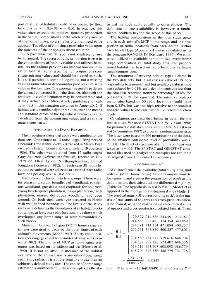
We transformed the available (total study area) and utilized (MCP home range) habitat compositions to log-ratios YO and y using the proportion of scrub as the denominator, then calculated the difference d = y- yO (Table 2). The hypothesis to test is d 0 (Model 2) as opposed to the more general situation d X 0 (Model 1). The residual matrix R2 corresponding to M2 is the matrix of raw sums of squares and cross-products calculated from d; R. is the matrix of mean-corrected sums of squares and cross-products calculated from d. Then:

179.527 214.586 244.591 273.761 214.586 268.435 314.354 343.859 244.591 314.354 471.084 400.237

R 273.761 343.859 400.237 477.801

IRJ 731.580 734.577 519.616 648.204 734.577 758.225 573.407 696.556 519.616 573.407 608.098 586.779 648.204 696.556 586.779 731.776

7 731 764 = 91051752 = 0.0849

91 051 752

and -N In A = - 13 ln(0.0849) = 32.06 yields P <


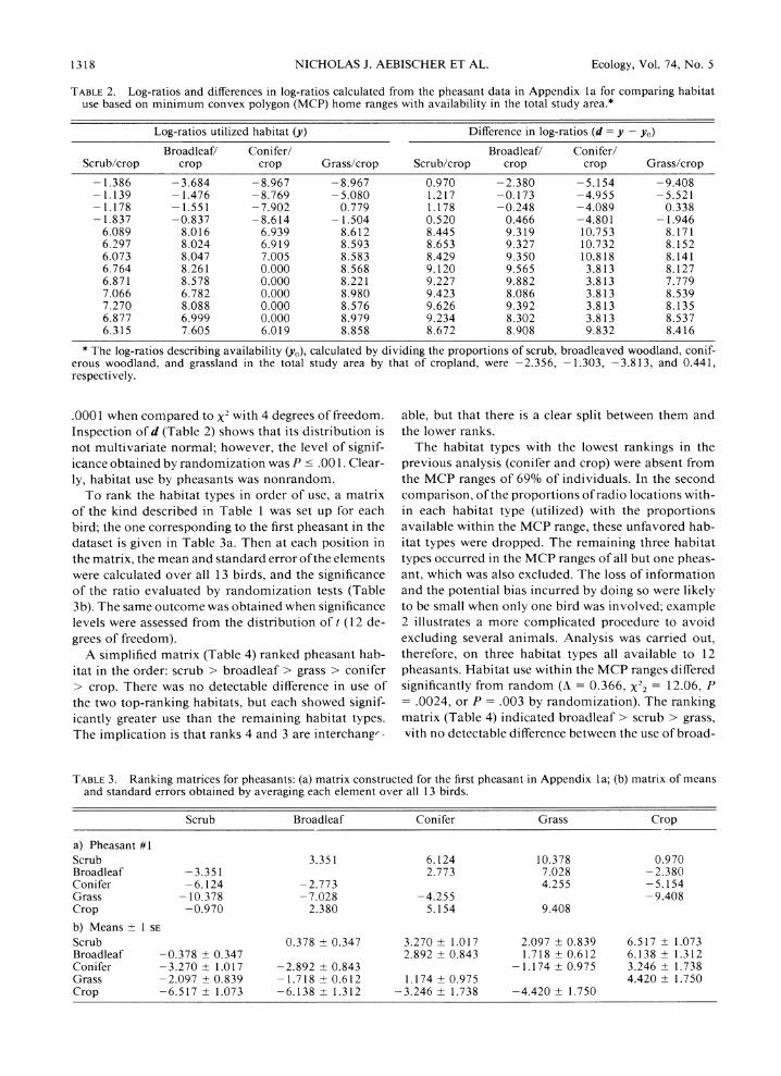
TABLE 2. Log-ratios and differences in log-ratios calculated from the pheasant data in Appendix la for comparing habitat use based on minimum convex polygon (MCP) home ranges with availability in the total study area.*

Log-ratios utilized habitat (y) Difference in log-ratios (d = y - yo)

Broadleaf/ Conifer/ Broadleaf/ Conifer/ Scrub/crop crop crop Grass/crop Scrub/crop crop crop Grass/crop

- 1.386 -3.684 -8.967 -8.967 0.970 -2.380 -5.154 -9.408 - 1.139 - 1.476 -8.769 - 5.080 1.217 -0.173 -4.955 -5.521 - 1.178 - 1.551 -7.902 0.779 1.178 -0.248 -4.089 0.338 - 1.837 -0.837 -8.614 - 1.504 0.520 0.466 -4.801 - 1.946

6.089 8.016 6.939 8.612 8.445 9.319 10.753 8.171 6.297 8.024 6.919 8.593 8.653 9.327 10.732 8.152 6.073 8.047 7.005 8.583 8.429 9.350 10.818 8.141 6.764 8.261 0.000 8.568 9.120 9.565 3.813 8.127 6.871 8.578 0.000 8.221 9.227 9.882 3.813 7.779 7.066 6.782 0.000 8.980 9.423 8.086 3.813 8.539 7.270 8.088 0.000 8.576 9.626 9.392 3.813 8.135 6.877 6.999 0.000 8.979 9.234 8.302 3.813 8.537 6.315 7.605 6.019 8.858 8.672 8.908 9.832 8.416

* The log-ratios describing availability (yo), calculated by dividing the proportions of scrub, broadleaved woodland, conif- erous woodland, and grassland in the total study area by that of cropland, were -2.356, -1.303, -3.813, and 0.441, respectively.

.0001 when compared to X2 with 4 degrees of freedom. Inspection of d (Table 2) shows that its distribution is not multivariate normal; however, the level of significance obtained by randomization was P c .001. Clear- ly, habitat use by pheasants was nonrandom.

To rank the habitat types in order of use, a matrix of the kind described in Table 1 was set up for each bird; the one corresponding to the first pheasant in the dataset is given in Table 3a. Then at each position in the matrix, the mean and standard error of the elements were calculated over all 13 birds, and the significance of the ratio evaluated by randomization tests (Table 3b). The same outcome was obtained when significance levels were assessed from the distribution of t (12 degrees of freedom).

A simplified matrix (Table 4) ranked pheasant habitat in the order: scrub > broadleaf > grass > conifer > crop. There was no detectable difference in use of the two top-ranking habitats, but each showed significantly greater use than the remaining habitat types. The implication is that ranks 4 and 3 are interchang-

able, but that there is a clear split between them and the lower ranks.

The habitat types with the lowest rankings in the previous analysis (conifer and crop) were absent from the MCP ranges of 69% of individuals. In the second comparison, of the proportions of radio locations within each habitat type (utilized) with the proportions available within the MCP range, these unfavored habitat types were dropped. The remaining three habitat types occurred in the MCP ranges of all but one pheasant, which was also excluded. The loss of information and the potential bias incurred by doing so were likely to be small when only one bird was involved; example 2 illustrates a more complicated procedure to avoid excluding several animals. Analysis was carried out, therefore, on three habitat types all available to 12 pheasants. Habitat use within the MCP ranges differed significantly from random (A = 0.366, X22 = 12.06, P = .0024, or P = .003 by randomization). The ranking matrix (Table 4) indicated broadleaf > scrub > grass, vith no detectable difference between the use of broad-

TABLE 3. Ranking matrices for pheasants: (a) matrix constructed for the first pheasant in Appendix la; (b) matrix of means and standard errors obtained by averaging each element over all 13 birds.

Scrub Broadleaf Conifer Grass Crop

a) Pheasant # 1 Scrub 3.351 6.124 10.378 0.970 Broadleaf -3.351 2.773 7.028 -2.380 Conifer -6.124 - 2.773 4.255 - 5.154 Grass - 10.378 -7.028 -4.255 -9.408 Crop -0.970 2.380 5.154 9.408

b) Means ? 1 SE

Scrub 0.378 ? 0.347 3.270 ? 1.017 2.097 ? 0.839 6.5 17 ? 1.073 Broadleaf -0.378 ? 0.347 2.892 ? 0.843 1.718 ? 0.612 6.138 ? 1.312 Conifer -3.270 ? 1.017 -2.892 ? 0.843 -1.174 ? 0.975 3.246 ? 1.738 Grass -2.097 0.839 -1.718 ? 0.612 1.174 ? 0.975 4.420 ? 1.750 Crop -6.517 ? 1.073 -6.138 ? 1.312 - 3.246 ? 1.738 -4.420 ? 1.750


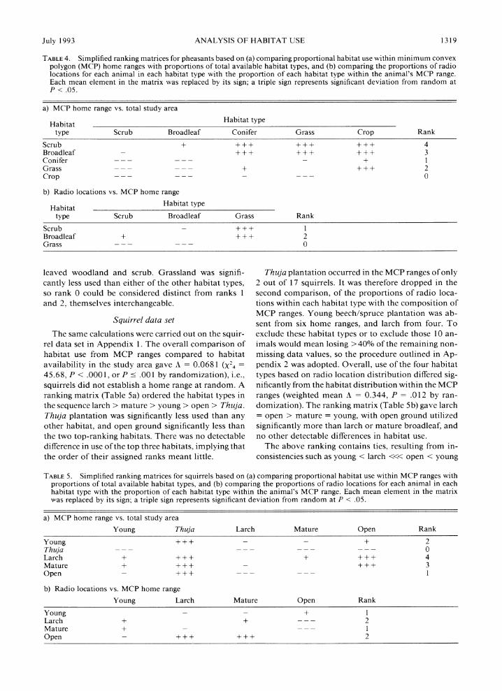
TABLE 4. Simplified ranking matrices for pheasants based on (a) comparing proportional habitat use within minimum convex polygon (MCP) home ranges with proportions of total available habitat types, and (b) comparing the proportions of radio locations for each animal in each habitat type with the proportion of each habitat type within the animal's MCP range. Each mean element in the matrix was replaced by its sign; a triple sign represents significant deviation from random at P < .05.

a) MCP home range vs. total study area

Habitat Habitat type type Scrub Broadleaf Conifer Grass Crop Rank

Scrub + + +-+ +++ +++ 4 Broadleaf --+ + + + + + + + + 3 Conifer --- --- - + 1 Grass - - - - - - + + + + 2 Crop ---

b) Radio locations vs. MCP home range

Habitat Habitat type type Scrub Broadleaf Grass Rank

Scrub - + + + 1 Broadleaf + + + + 2 Grass --- --- 0

leaved woodland and scrub. Grassland was significantly less used than either of the other habitat types, so rank 0 could be considered distinct from ranks 1 and 2, themselves interchangeable.

Squirrel data set

The same calculations were carried out on the squirrel data set in Appendix 1. The overall comparison of habitat use from MCP ranges compared to habitat availability in the study area gave A = 0.0681 (X24 =

45.68, P < .0001, or P < .001 by randomization), i.e., squirrels did not establish a home range at random. A ranking matrix (Table 5a) ordered the habitat types in the sequence larch > mature > young > open > Thuja. Thuja plantation was significantly less used than any other habitat, and open ground significantly less than the two top-ranking habitats. There was no detectable difference in use of the top three habitats, implying that the order of their assigned ranks meant little.

Thuja plantation occurred in the MCP ranges of only 2 out of 17 squirrels. It was therefore dropped in the second comparison, of the proportions of radio locations within each habitat type with the composition of MCP ranges. Young beech/spruce plantation was absent from six home ranges, and larch from four. To exclude these habitat types or to exclude those 10 animals would mean losing > 40% of the remaining nonmissing data values, so the procedure outlined in Ap- pendix 2 was adopted. Overall, use of the four habitat types based on radio location distribution differed significantly from the habitat distribution within the MCP ranges (weighted mean A = 0.344, P = .012 by randomization). The ranking matrix (Table 5b) gave larch = open > mature = young, with open ground utilized significantly more than larch or mature broadleaf, and no other detectable differences in habitat use.

The above ranking contains ties, resulting from in- consistencies such as young < larch <<< open < young

TABLE 5. Simplified ranking matrices for squirrels based on (a) comparing proportional habitat use within MCP ranges with proportions of total available habitat types, and (b) comparing the proportions of radio locations for each animal in each habitat type with the proportion of each habitat type within the animal's MCP range. Each mean element in the matrix was replaced by its sign; a triple sign represents significant deviation from random at P < .05.

a) MCP home range vs. total study area

Young Thuja Larch Mature Open Rank

Young + +-+ - - + 2 Thuja - --- - --- 0 Larch + + +-+ + + + + 4 Mature + + + + - +++ 3 Open - +++ --- --- I

b) Radio locations vs. MCP home range

Young Larch Mature Open Rank

Young - - A- Larch + + --- 2 Mature + -I Open - +A++ +A++ 2


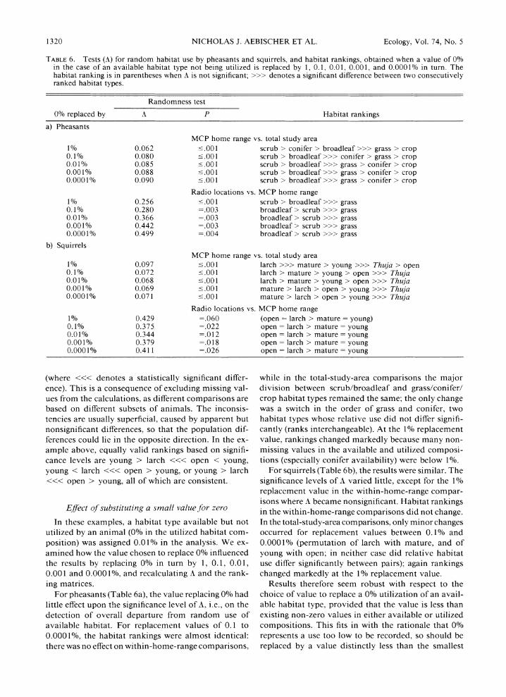
TABLE 6. Tests (A) for random habitat use by pheasants and squirrels, and habitat rankings, obtained when a value of 0% in the case of an available habitat type not being utilized is replaced by 1, 0.1, 0.01, 0.001, and 0.0001 /% in turn. The habitat ranking is in parentheses when A is not significant; >>> denotes a significant difference between two consecutively ranked habitat types.

Randomness test

0% replaced by A P Habitat rankings

a) Pheasants

MCP home range vs. total study area 1% 0.062 ?.001 scrub > conifer > broadleaf >>> grass > crop 0.11% 0.080 ? 001 scrub > broadleaf >>> conifer > grass > crop 0.01% 0.085 ?001 scrub > broadleaf >>> grass > conifer > crop 0.001% 0.088 <.001 scrub > broadleaf >>> grass > conifer > crop 0.0001% 0.090 ?<.001 scrub > broadleaf >>> grass > conifer > crop

Radio locations vs. MCP home range 10% 0.256 ?<.001 scrub > broadleaf >>> grass 0.1I % 0.280 =.003 broadleaf > scrub >>> grass 0.01% 0.366 =.003 broadleaf > scrub >>> grass 0.001% 0.442 =.003 broadleaf > scrub >>> grass 0.00010% 0.499 =.004 broadleaf > scrub >>> grass

b) Squirrels MCP home range vs. total study area

1% 0.097 <.001 larch >>> mature > young >>> Thuja > open 0.1% 0.072 <.001 larch > mature > young > open >>> Thuja 0.01% 0.068 <.001 larch > mature > young > open >>> Thuja 0.001% 0.069 <.001 mature > larch > open > young >>> Thuja 0.0001% 0.071 <.001 mature > larch > open > young >>> Thuja

Radio locations vs. MCP home range 1% 0.429 =.060 (open larch > mature young) 0.1% 0.375 =.022 open larch > mature young 0.01% 0.344 =.012 open larch > mature young 0.001% 0.379 =.018 open larch > mature young 0.0001% 0.411 =.026 open larch > mature young

(where <<< denotes a statistically significant difference). This is a consequence of excluding missing values from the calculations, as different comparisons are based on different subsets of animals. The inconsis- tencies are usually superficial, caused by apparent but nonsignificant differences, so that the population differences could lie in the opposite direction. In the example above, equally valid rankings based on significance levels are young > larch <<< open < young, young < larch <<< open > young, or young > larch <<< open > young, all of which are consistent.

Effect of substituting a small value for zero

In these examples, a habitat type available but not utilized by an animal (0% in the utilized habitat composition) was assigned 0.01% in the analysis. We ex- amined how the value chosen to replace 0% influenced the results by replacing 0% in turn by 1, 0.1, 0.01, 0.001 and 0.0001 %, and recalculating A and the ranking matrices.

For pheasants (Table 6a), the value replacing 0% had little effect upon the significance level of A, i.e., on the detection of overall departure from random use of available habitat. For replacement values of 0.1 to 0.0001%, the habitat rankings were almost identical: there was no effect on within-home-range comparisons,

while in the total-study-area comparisons the major division between scrub/broadleaf and grass/conifer/ crop habitat types remained the same; the only change was a switch in the order of grass and conifer, two habitat types whose relative use did not differ significantly (ranks interchangeable). At the 1% replacement value, rankings changed markedly because many nonmissing values in the available and utilized compositions (especially conifer availability) were below 1%.

For squirrels (Table 6b), the results were similar. The significance levels of A varied little, except for the 1% replacement value in the within-home-range comparisons where A became nonsignificant. Habitat rankings in the within-home-range comparisons did not change. In the total-study-area comparisons, only minor changes occurred for replacement values between 0.10% and 0.0001% (permutation of larch with mature, and of young with open; in neither case did relative habitat use differ significantly between pairs); again rankings changed markedly at the 1% replacement value.

Results therefore seem robust with respect to the choice of value to replace a 0% utilization of an available habitat type, provided that the value is less than existing non-zero values in either available or utilized compositions. This fits in with the rationale that 0% represents a use too low to be recorded, so should be replaced by a value distinctly less than the smallest


nonzero value: an order of magnitude less is probably appropriate to most situations.

DISCUSSION

Radiotelemetry is one of the most powerful tools available to the wildlife biologist because of its potential for providing unbiased data on an animal's use of time and space. However, the analysis of habitat use is not straightforward, owing to the problems of sampling level, unit-sum constraint, differential use, and definition of availability.

In this paper, we countered these problems by ob- serving that an animal's habitat use is determined by its trajectory, subsampled by radiotelemetry. Although the number of radio locations per animal determines the accuracy with which its habitat use is estimated, it is the number of animals tracked that determines the sample size upon which to base and test hypotheses concerning habitat use by the population; use of radio locations as the sample size constitutes pseudoreplication (Hurlbert 1984). For each animal, habitat use (and availability) is given by a set of proportions describing habitat composition. A statistical tool appropriate to multivariate data which sum to 1 is compositional analysis (Aitchison 1986), which can test the same range of hypotheses as multivariate regression and MANOVA. We demonstrated how to compare habitat use with availability, one of the most common requirements in habitat analysis. In this case, the analysis is closely related to Johnson's (1980) rank-based method. However, compositional analysis extends to more complicated analyses of habitat use, for example a two-way classification by sex and age, a blocked design with data collected in different years or sites, a relationship between habitat use and food abundance or the presence of other animal species.

What are the design implications for radiotelemetry studies of habitat use? Obviously, sample sizes must be adequate for statistical analysis. We note that if values of a log-ratio difference (Table 3) all have the same sign, 6 is the minimum sample size required to show a significant difference from zero at P < .05 by randomization (Siegel 1956). So for a comparison of utilized with available habitats, 6 radio-tagged animals constitute an absolute minimum. We recommend sample sizes above 10, and preferably above 30, to represent a population adequately. The examples pre- sented in this paper are therefore borderline in this respect. For comparisons between categories of animals, each category should exceed 10 individuals. Un- less seasonal effects can be ignored or are modelled explicitly in the analysis, tracking of all animals should take place during the same period. Replication across sites or years is possible within the framework of compositional analysis, as site and year effects can be in- corporated into the fitted model.

The cost and effort involved in monitoring large

numbers of animals may be partially offset by auto- matic data collection or by reducing the number of radio locations collected per animal. The optimal al- location of resources among animals and radio locations per animal depends on the extent to which animals behave differently (between-animal variation) and how accurately an animal's habitat use is estimated (subsampling efficiency). The principle is the same as for a mixed-model nested ANOVA (Sokal and Rohlf 1981). In essence, as between-animal variation increases, it affects the accuracy of the mean more than in- accurate estimates of an individual's habitat use. In this situation, increasing the number of animals im- proves the accuracy of the mean even if the number of radio locations is reduced. A pilot study is useful to determine between-animal variation and subsampling efficiency; if home-range estimates are needed, it also assesses their stability in relation to number of radio locations (Kenward 1982, 1992, Parish and Kruuk 1982, Harris et al. 1990).

Another point is that radio locations collected from an animal must provide an unbiased representation of the trajectory they sample. Locating the animal either at random times or at regular intervals throughout the study period achieves this. So do more complicated methods based on intensive monitoring during short periods on different days, as long as overall sampling intensity is uniform. If sampling is at regular intervals, the interval must be chosen so that it is not a multiple of some cycle in the animal's behavior.

Several assumptions underlie the compositional analysis of habitat use (Aitchison 1986). An important one is that each animal provides an independent measure of habitat use within the population. Caution is needed if animals are gregarious. Territoriality too may influence the position of an animal's home range with respect to the overall study area, but should not in- validate a within-home-range comparison of utilized with available habitat. Another assumption that can affect model-fitting is that compositions from different animals are equally accurate, which is untrue if numbers of radio locations vary widely from animal to animal. If such is the case, then during analysis the log- ratios derived from each animal's habitat composition should be weighted by a quantity related to the corresponding number of radio locations, n. If locations are independent, the variance of the proportion in each habitat type is inversely related to ni, but in case of autocorrelation, the effective number will be lower. Weighting by the full number of locations might also give too much emphasis to frequently observed animals (Alldredge and Ratti 1992); a suitable compro- mise might be to weight by the square root of n. A third assumption affecting standard hypothesis testing is that of multivariate normality of the residuals after model fitting. However, failure of this assumption in- fluences only the significance levels, not the fitting of models to log-ratio data nor the calculation of statistics;


significance levels are obtainable free of distributional assumptions by randomization (Manly 199 1).

The logarithmic transformation underpinning compositional analysis requires that each animal use all habitat types. Often, however, the proportional habitat use is estimated as zero. If the zero represents use so low that it has not been detected, the solution adopted here is to substitute some small value. The examples suggest that the substitution produces results that are robust relative to the substituted value, provided that it is lower than the smallest nonzero value recorded. For the purpose of comparing usage with availability, Johnson's (1 980) ranking method requires no such substitution. The use of ranks results, however, in loss of information and sensitivity (Alldredge and Ratti 1986), and the method does not extend to ANCOVA-type linear modelling. If the proportional habitat use is zero because the corresponding habitat type is not available, the zero provides no information on use and should be regarded as a missing value whatever analytical procedure is adopted; any attempt to assign a value (or a rank) to such a zero is arbitrary and likely to bias the results. Compositional analysis can be applied using the procedure in Appendix 2, but asymmetries in the data matrix can produce ill-defined rankings.

We do not pretend that compositional analysis is the ultimate solution to analyzing habitat use. What we wish to emphasize is that it provides a statistically sound basis and flexible modelling capability for such analyses. Many other "simpler" methods violate key assumptions or ignore the particular structure of data on habitat use. The level of bias generated because of that is always difficult to assess, and the results are correspondingly untrustworthy, even though they may appear (or even be) sensible. As a general statistical technique aimed at proportional data (Aitchison 1986), compositional analysis is clearly suited to the analysis of habitat use and answers problems 1 to 3. The per- formance of the technique remains to be evaluated, as the only true yardstick is simulated data based on known parameters. Simulation could provide a critical assessment of the power of the test and of the impact of zero proportions. It would also give valuable insight into questions of sample size and experimental design, for instance the trade-off between number of animals and number of radio locations per animal, or the relationship, if any, between number of animals and number of habitat types.

Regarding a comparison of habitat use with availability (Problem 4), we consider that use operates in two stages, corresponding to the selection levels 2 and 3 of Johnson (1980). This reduces the effects of an arbitrary definition of study area (Porter and Church 1987), and also provides insights into the way animals use their habitat. However, fundamental problems re- main. Not only is the choice of study area arbitrary, but the same is also true of the method of evaluating home range. We are not recommending the use of min-

imum convex polygons or any other home range estimator as a true reflection of the area of habitat actually available to an animal. Rather, the home range estimate is a useful method of separating utilization into two stages and avoiding the more serious conse- quences of relying solely on an arbitrarily defined study area. Different results would be obtained by using different home range estimators; we are currently investigating how different estimators, based on discontin- uous radio locations, relate to the underlying animal trajectory.

A two-stage approach to habitat use has considerable advantages. For instance, squirrels are typically woodland animals, and, in their selection of MCP ranges from within the overall study area, they made little use of open ground (Table 5). However, when considering the distribution of radio locations within the MCP ranges, open ground tied with larch as the most used habitat type. This was because the animals were for- aging for food in a wheat field adjacent to the wood. Such an effect is apparent only if selection is considered to act in two stages. A comparison of radio location distribution with overall habitat availability within the study area would have ranked open ground as a rarely used habitat type even though it provided an important food resource.

The potential of compositional analysis extends beyond questions of habitat use. For instance, activity budgets pose almost identical problems in analysis. The individual animal is the level at which to test population hypotheses, although measuring budgets often involves point sampling of ongoing activities. If so, the more frequent the sampling, the more accurate the determination of the animal's budget; the most accurate determination is when activity is recorded continuously, as by direct observation or video film. The data from an individual should be expressed as proportions of time spent on each activity, i.e., as an activity composition; analysis is then as for habitat compositions. Similarly, compositional analysis is relevant to the analysis of diet (where consumption may be expressed in terms oL proportions of different food items) and to several other areas of biological interest.

ACKNOWLEDGMENTS

We thank the National Association of Regional Game Councils and the Irish Forestry and Wildlife Department for funding the collection of the pheasant data. We are grateful to R. T. Clarke, G. R. Potts, J. C. Reynolds, and S. C. Tapper for discussions on the methodology, and to M. G. Morris for comments on the manuscript. We also thank K. P. Burnham, D. H. Johnson, and G. C. White for their encouraging and helpful criticisms.

LITERATURE CITED

Aitchison, J. 1986. The statistical analysis of compositional data. Chapman and Hall, London, England.

Alldredge, J. R., and J. T. Ratti. 1986. Comparison of some statistical techniques for analysis of resource selection. Journal of Wildlife Management 50:157-165.

Alldredge, J. R., and J. T. Ratti. 1992. Further comparison


of some statistical techniques for analysis of resource selection. Journal of Wildlife Management 56:1-9.

Byers, C. R., R. K. Steinhorst, and P. R. Krausman. 1984. Clarification of a technique for analysis of utilization-availability data. Journal of Wildlife Management 48:1050-1053.

Carmer, S. G., and M. R. Swanson. 1973. An evaluation of ten pairwise multiple comparison procedures by Monte Carlo methods. Journal of the American Statistical Association 68:66-74.

Cox, D. R., and D. V. Hinkley. 1974. Theoretical statistics. Chapman and Hall, New York, New York, USA.

Dixon, K. R., and J. A. Chapman. 1980. Harmonic mean measure of animal activity areas. Ecology 61:1040-1044.

Dobson, A. J. 1983. Introduction to statistical modelling. Chapman and Hall, New York, New York, USA.

Friedman, M. 1937. The use of ranks to avoid the assumption of normality implicit in the analysis of variance. Jour- nal of the American Statistical Association 32:675-701.

Genstat 5 Committee. 1987. Genstat 5 reference manual. Oxford University Press, New York, New York, USA.

Harris, S., W. J. Cresswell, P. G. Forde, W. J. Trewhella, T. Woollard, and S. Wray. 1990. Home-range analysis using radio-tracking data-a review of problems and techniques particularly as applied to the study of mammals. Mammal Review 20:97-123.

Heisey, D. M. 1985. Analyzing selection experiments with log-linear models. Ecology 66:1744-1748.

Hogg, R. V., and A. T. Craig. 1970. Introduction to math- ematical statistics. Third edition. Macmillan, New York, New York, USA.

Hurlbert, S. H. 1984. Pseudoreplication and the design of ecological field experiments. Ecological Monographs 54: 187-211.

Jennrich, R. J., and F. B. Turner. 1969. Measurement of non-circular home range. Journal of Theoretical Biology 22:227-237.

Johnson, D. H. 1980. The comparison of usage and availability measurements for evaluating resource preference. Ecology 61:65-7 1.

Kenward, R. E. 1982. Techniques for monitoring the be- haviour of Grey Squirrels by radio. Symposium of the Zoo- logical Society of London 49:175-196.

1987. Wildlife radio tagging: equipment, field techniques and data analysis. Academic Press, Orlando, Flor- ida, USA.

* 1990. RANGES IV. Software for analysing animal location data. Institute of Terrestrial Ecology, Natural En- vironment Research Council, Cambridge, England.

1992. Quantity versus quality: programmed collection and analysis of radio-tracking data. Pages 231-246 in I. G. Priede and S. M. Swift, editors. Wildlife telemetry: remote monitoring and tracking of animals. Ellis Horwood, New York, New York, USA.

Manly, B. F. J. 1991. Randomization and Monte Carlo methods in biology. Chapman and Hall, New York, New York, USA.

Mohr, C. 0. 1947. Table of equivalent populations of North American small mammals. American Midland Naturalist 37:223-249.

Morrison, D. F. 1990. Multivariate statistical methods. Third edition. McGraw-Hill, New York, New York, USA.

Neu, C. W., C. R. Byers, and J. M. Peek. 1974. A technique for analysis of utilization-availability data. Journal of Wild- life Management 38:541-545.

Parish, T., and H. Kruuk. 1982. The uses of radio tracking combined with other techniques in studies of badger ecology in Scotland. Symposium of the Zoological Society of London 49:291-299.

Porter, W. F., and K. E. Church. 1987. Effects of environ- mental pattern on habitat preference analysis. Journal of Wildlife Management 51:681-685.

Quade, D. 1979. Using weighted rankings in the analysis of complete blocks with additive block effects. Journal of the American Statistical Association 74:680-683.

Robertson, P. A. 1986. The ecology and management of hand-reared and wild pheasants (Phasianus colchicus) in Ireland. Dissertation. National University of Ireland, Dub- lin, Ireland.

Siegel, S. 1956. Nonparametric statistics for the behavioral sciences. McGraw-Hill, New York, New York, USA.

Smith, L. M., J. W. Hupp, and J. T. Ratti. 1982. Habitat use and home range of gray partridge in eastern South Da- kota. Journal of Wildlife Management 46:580-587.

Snedecor, G. W., and W. G. Cochran. 1980. Statistical methods. Seventh edition. Iowa State University Press, Ames, Iowa, USA.

Sokal, R. R., and F. J. Rohlf. 1981. Biometry. Second edition. W. H. Freeman, San Francisco, California, USA.

Swihart, R. K., and N. A. Slade. 1985a. Testing for independence of observations in animal movements. Ecology 66:1176-1184.

Swihart, R. K., and N. A. Slade. 1985b. Influence of sampling interval on estimates of home-range size. Journal of Wildlife Management 49:1019-1025.

White, G. C., and R. A. Garrott. 1990. Analysis of wildlife radiotracking data. Academic Press, San Diego, California, USA.

Wiens, J. A. 1973. Pattern and process in grassland bird communities. Ecological Monographs 43:237-270.

Wilkinson, L. 1990. SYSTAT: the system for statistics. Sy- stat, Evanston, Illinois, USA.

Worton, B. J. 1989. Kernel methods for estimating the utilization distribution in home-range studies. Ecology 70: 164-168.


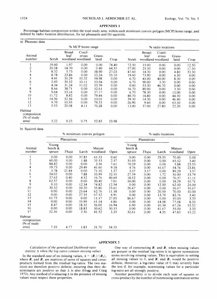
APPENDIX 1

Percentage habitat composition within the total study area, within each minimum convex polygon (MCP) home range, and defined by radio location distribution, for (a) pheasants and (b) squirrels.

a) Pheasant data

% MCP home range % radio locations

Broad Conif- Broad- Conif- Animal leaf erous Grass- leaf erous Grass- number Scrub woodland woodland land Crop Scrub woodland woodland land Crop

1 19.60 1.97 0.00 0.00 78.40 72.50 15.00 0.00 0.00 12.50 2 20.58 14.70 0.00 0.40 64.31 57.00 25.50 0.00 0.00 17.50 3 8.32 5.73 0.00 58.90 27.03 47.60 14.30 0.00 4.80 33.30 4 8.78 23.86 0.00 12.24 55.10 19.60 73.90 0.00 6.50 0.00 5 4.41 30.29 10.32 54.98 0.00 6.70 45.00 40.00 8.30 0.00 6 5.43 30.52 10.11 53.94 0.00 6.70 90.00 3.30 0.00 0.00 7 4.34 31.24 11.02 53.39 0.00 0.00 53.30 46.70 0.00 0.00 8 8.66 38.71 0.00 52.61 0.00 16.70 80.00 0.00 3.30 0.00 9 9.64 53.16 0.00 37.17 0.00 6.70 78.30 0.00 15.00 0.00

10 11.72 8.82 0.00 79.44 0.00 40.70 14.80 0.00 44.50 0.00 11 14.36 32.56 0.00 53.05 0.00 39.30 14.30 0.00 46.40 0.00 12 9.70 10.95 0.00 79.33 0.00 26.90 9.60 0.00 63.50 0.00 13 5.53 20.08 4.11 70.28 0.00 13.00 37.00 27.80 22.20 0.00

Habitat composition (% of study area) 3.22 9.23 0.75 52.83 33.98

b) Squirrel data

% minimum convex polygon % radio locations

Plantations Plantations

Young Young Animal beech & Mature beech & Mature number spruce Thuja Larch woodland Open spruce Thuja Larch woodland Open

1 0.00 0.00 37.85 61.53 0.60 0.00 0.00 29.55 70.45 0.00 2 60.00 0.00 1.88 35.53 2.57 31.03 0.00 0.00 65.52 3.45 3 88.82 0.00 0.00 3.56 7.61 70.59 0.00 0.00 5.88 23.53 4 19.73 0.00 29.49 41.60 9.18 4.76 0.00 16.67 54.76 23.81 5 5.78 21.84 0.00 71.10 1.27 3.57 3.57 0.00 89.29 3.57 6 24.02 0.00 7.88 35.99 32.10 27.59 0.00 1.72 56.90 13.79 7 37.63 0.40 4.52 16.76 40.69 18.52 0.00 0.00 70.37 11.11 8 62.57 0.00 0.00 30.40 7.01 50.00 0.00 0.00 39.29 10.71 9 0.10 0.00 12.54 74.82 12.54 0.00 0.00 12.50 62.50 25.00

10 30.32 0.00 10.20 35.86 23.61 26.67 0.00 0.00 56.67 16.67 11 0.00 0.00 25.64 62.76 11.58 0.00 0.00 20.00 70.00 10.00 12 0.00 0.00 27.55 67.52 4.91 0.00 0.00 13.79 82.76 3.45 13 61.75 0.00 0.00 11.17 27.05 86.67 0.00 0.00 10.00 3.33 14 0.00 0.00 33.99 61.14 4.86 0.00 0.00 14.58 77.08 8.33 15 8.47 0.00 18.52 56.05 16.94 6.90 0.00 10.34 67.24 15.52 16 0.00 0.00 18.83 50.62 30.53 0.00 0.00 41.67 55.00 3.33 17 52.56 0.00 2.56 41.52 3.35 32.61 0.00 4.35 47.83 15.22

Habitat composition (% of study area) 7.35 4.77 1.83 31.70 54.35

APPENDIX 2

Calculation of the generalized likelihood-ratio statistic A when the log-ratios contain missing values

In the standard case of no missing values, A = I R. /j R2I , where R. and R. are matrices of sums of squares and cross- products formed from the residual log-ratios. The two matrices are therefore positive definite, ensuring that their de- terminants are positive so that A is also (Hogg and Craig 1970). Any method of evaluating A in the presence of missing values must respect these properties.

One way of constructing R. and R2 when missing values are present in the residual log-ratios is to ignore summation terms involving missing values. This is equivalent to setting all missing values to 0, and R. and R, would be positive definite. However, a log-ratio value of 0 may severely bias the test if, for example, nonmissing values for a particular log-ratio are all strongly positive.

Another possibility is to divide each sum of squares or cross-product by the number of nonmissing summation terms


entering it, thus producing a variance-covariance matrix based on nonmissing values. However, the unbalanced nature of missing values results in matrices that are not necessarily positive definite and can produce invalid values for A.

A third, preferred, option is to replace the missing values in a particular residual log-ratio by the mean of all nonmissing values for that log-ratio. A matrix of sums of squares and cross-products calculated from such log-ratios is positive definite; the substitution also has the property that the mean of each log-ratio is the same after substitution as before. This is particularly relevant in the comparison of utilized with available habitat, as the log-ratio means are used to build a ranking matrix.

Based on the above substitution, A can be evaluated suc- cessfully. However, its value will no longer be independent of the habitat type chosen as denominator in the initial transformation to log-ratios, because missing values in the log- ratios result from missing values in the denominator as well as in the numerator. Furthermore, A is no longer likely to conform to the standard x2 distribution. We suggest com- puting a mean A by weighting each denominator-dependent value of A by the number of nonmissing values involved in its calculation, and determining the level of significance by randomization. It is important that during each cycle in the randomization procedure, substitution of missing values in a log-ratio by the mean of the nonmissing values for that log- ratio be performed after randomization of the log-ratio values.

Documents

Compositional Analysis of Habitat Use From Animal … · COMPOSITIONAL ANALYSIS OF HABITAT USE FROM ... Fordingbridge, Hampshire SP6 JEF United Kingdom ... Jennrich and Turner 1969;