Composite System Reliability Analysis UsingParticle Swarm Optimization

Joydeep Mitra, Senior Member, IEEE, and Xufeng XuDepartment of Electrical & Computer Engineering

Michigan State UniversityEast Lansing, Michigan 48824, USA

mitraj@msu.edu, xufeng@egr.msu.edu

Abstract—This paper presents a new approach to compositesystem reliability analysis. This approach is based on multi-objective particle swarm optimization (PSO), which is used as anintelligent method for scanning the state space. This paper adaptstraditional binary PSO to bi-objective binary PSO using loadcurtailment and state probability as the two objectives to bettercontrol the particle dynamics. Another novel feature of thismethod is that while it utilizes information from failure states toestimate loss of load indices, it also uses information fromacceptable states that are encountered to accelerate theconvergence of the estimate. The method is demonstrated on themodified IEEE Reliability Test System. It is also shown tocompare very favorably with Monte Carlo Simulation.

Keywords— composite system, reliability evaluation, multi-objective particle swarm optimization.

I. INTRODUCTION

omposite system reliability evaluation consists ofdetermining the reliability of a power system taking into

account both its generation and its transmission components. Itcan also be viewed as a combined adequacy and securityanalysis, and is appropriate in systems where the internaltransmission constraints play a significant role in determiningoverall system reliability [1]. In general, composite systemreliability methods permit the determination of system-wide aswell as locational reliability indices, and can be used forplanning and operation studies.

Traditionally, analytical [2–4] and Monte Carlo [5], [6]methods have been used for composite system reliabilityevaluation. While analytical techniques are potentially faster,they tend to get difficult as system size and complexityincreases. Monte Carlo methods, on the other hand, affordtremendous modeling flexibility, and can be used for systemswith large size and complexity. However, Monte carlomethods tend to be extremely time consuming, particularly forreliable systems. For this reason, in recent years severalmethods have been proposed, based on so calledcomputational intelligence or heuristic search methods. Recentwork has used genetic algorithms (GA) [7], [8], artificialneural networks (ANN) [9], and particle swarm optimization(PSO) [10]. These approaches have generally performed well

in terms of computational accuracy, and have often beenreported to be faster than traditional, i.e., analytical and MonteCarlo based methods.

This paper presents an innovative method of computingreliability indices of composite systems, and is based on amulti-objective particle swarm formulation. It uses twoobjectives—load curtailment and failure probability—as twoobjectives in the PSO fitness to exercise better control over theparticle dynamics. A further innovation in this work consistsof using information from acceptable system states toaccelerate the convergence of indices determined from systemfailure states. Hence in this approach, both loss of loadprobability (LOLP) and availability (denoted “NLOLP”hereafter) of the system are calculated during the searchprocess. Based on the trends of the successive estimates of thetwo indices, accelerated estimates of the LOLP are obtainedusing three different methods.

The IEEE Reliability Test System (RTS) [11] is used fortesting the method. However, since the original IEEE-RTSwas shown to be of limited use for composite system studieson account of its transmission system being too strong [12], itsdata was suitably modified. The proposed method is shown tocompare favorably with prior methods.

II. LOSS OF LOAD PROBABILITY ESTIMATION

This work uses the LOLP as the reliability index ofcomposite system, since it reflects the risk of the generationcapacity failing to satisfy the load demand in the presence oftransmission constraints and contingencies. Several factorshave impact on LOLP, for example, component failure rate,network topology, generator dispatch, load demand, etc. Thesystem LOLP can be obtained by following formula:

Si

ipLOLP (1)

iSWj

j

iSRj

j

iSWj

j

iSRj

ji PLPLPGPGp 11 (2)

whereS is the set of states for which there is load curtailment;pi is probability of state i;R(Si) and W(Si) are the component sets in up or down states,respectively;

C

The work reported here was supported in part by the US National ScienceFoundation under Grant ECCS-0702208.

PGj or PLj is the failure probability of generating unit j ortransmission line j.

In this work, we use another index that we denote asNLOLP, which estimates the system availability. According to

our definition, NLOLP is always equal to 1– LOLP.

The system state is decided by generating unit and linestates. Most components in a composite system, such asgenerating units, lines, etc, can be can be modeled as twostates units, i.e., any component can be “up” or “down”. So thetotal number of states in a system will be 2m where m is thenumber of components in the system. For a system of realisticsize, the number of states will be extremely large; however,most of those states play a small role in reliability evaluation.Some heuristic approaches get enough precision throughvisiting sufficient states of high probability and this approachhas been shown to be effective.

III. THE DC FLOW MODEL AND LOAD CURTAILMENT

State analysis is the main part of composite systemreliability evaluation, and it can be divided into three steps: (1)first calculate power flow, and decide if there are any failuresituations, such as system disconnection and operationconstraint violation; (2) next try to fix the failure throughadjusting generator output; (3) finally, minimize loadcurtailment using the following redispatch model [13].

N

i

iC1

Min (3)

Subject to:DCGB (4)maxmin GGG (5)

DC 0 (6)maxff (7)

whereN is the number of system nodes;B is the nodal admittance matrix;

is the vector of bus voltage angles;G is the vector of dispatched generation output at all buses andlies in the interval [Gmin, Gmax];D and C are vectors of bus load demand and bus loadcurtailment, respectively;f is the vector of branch power flows and fmax is the vector ofbranch capacities.

If we define G and as the variables of this optimization

model and E the row vector N11,1,1 , and then (3) can be

rewritten as (8), shown below, by the substitution of (4). Byusing simple algebraic operations, constraints (4)–(7) can beconverted into equation (9), where I is a unit diagonal matrix,A is the branch-node incidence matrix, and b is the branchadmittance matrix. So the load curtailment problem can betransformed into a linear programming problem.

EDG

EBE

Min (8)

Subject to:min

max

max

max

0

0

0

0

0

I G

I G

I B G D

I B

bA f

bA f

(9)

IV. DESCRIPTION OF THE APPROACH

A. Bi-Objective Particle Swarm Optimization

The particle swarm optimization (PSO) was originated fromsimulation of social animal's behavior, such as bird and fish,and was put forward by Kennedy and Eberhart [14]. A discretebinary particle swarm optimization (BPSO) was proposed bythem for the purpose of solving combinatorial optimizationproblems [15].

PSO has been shown to have good performance in searchability, thus we use BPSO as a state searching tool and try tofind states which have an influence on system reliability indexas much as possible in a large state space. The best case iswhere particles only visit states which cause load curtailmentand have high probability at the same time. The problem isthat high consequence states (where many components arefailed) usually have low probability. There are two directionsof particles during the searching process: one is related to loadcurtailment and the other is related to state probability. Inorder to solve this problem, Particles that we design in thispaper will take both directions into consideration.

The particle velocity vi is the direction of movement ofparticle i from position xi in one time step, and is given by thefollowing [15]:

i

ii

i

iiii

xCgbestcrand

xCpbestcrand

xPgbestcrand

xPpbestcrandvv

4

3

2

1

()

()

()

()

(10)

where

iPpbest is the best position, in terms of highest state

probability, that particle i has ever encountered;

Pgbest is the position with the highest state probability

encountered by any particle;

iCpbest is the best position, in terms of highest load

curtailment, that particle i has ever encountered;

Cgbest is the position with the highest load curtailment

encountered by any particle;

1c , 2c , 3c and 4c are acceleration factors;

()rand is a uniformly distributed value in the interval 1,0 .

B. The Solution Algorithm

Our approach is mainly composed of three parts: statesampling, reliability index counting, and state analysis as

explained in section III. The whole reliability evaluationprocess can be divided into the following steps:1) Initialize the particle positions x and velocities v. Binary

numbers can be used to represent particles, 1 or 0represent up or down status respectively. The number ofbits equals to total number of generating units and lines.So each particle is corresponding to a certain system state.

2) For each particle in position xi, use (2) to compute theexact state probability.

3) Determine whether particle probability pi is smaller than, where is a predetermined threshold (very small)value. If so, go to the next step; otherwise, go to the nextparticle and continue to search. The threshold is apredetermined positive value and its value is determinedaccording to two aspects: on one hand, it is related tocomputing accuracy directly; on the other hand, as somestates with low probability plays a great role in thedecision of particle direction, so is unlikely be a largenumber.

4) Compute the equivalent decimal value of each particle toenable storage in the state database. In order to avoid thesituation that equivalent decimal value is too large, all bitsin xi can be divided into several groups, and then theequivalent decimal value can be computed for each group.

5) If the state (or particle position) already exists in database,set the probability of this particle to a small enough value(in our approach, we use ) and load curtailment to zero,and then go to step 9). If not, add decimal value, xi, pi, andload curtailment to database and go to the next step.

6) As xi contains status information of generating units andlines, update matrices B(xi), fmax(xi) and Gmax(xi)accordingly. Then analyze state according to the approachproposed in section III. If load shedding is inevitable,using optimal load curtailment model to cut load as shownin (8) and (9).

7) If there is load shedding, then add pi to the LOLPestimate, otherwise add pi to the NLOLP estimate.

8) If all particles have been processed, go to next step;Otherwise, go to step 3).

9) Initialize or update iPpbest , Pgbest , iCpbest and

Cgbest , and then update particle velocity iv using (10).

Bit d of Particle position xi is changed by following rule.

otherwisexe

randx

id

idvid

,01

1(),1

(11)

10) Test for convergence; if the estimate has converged, stopthe iteration when the index is stable; otherwise, go tostep 2).

C. Convergence Criterion

In the approach described above, two opposing criteria areused to control the particle dynamics and ensure that theparticles do not rapidly collapse to one corner of the searchspace. It is new appropriate to define a criterion for stoppingthe search process. Two estimates, LOLP and NLOLP arederived. Both LOLP and NLOLP are monotonically increasing

functions of n, the number of visited states. In each iteration k,we perform the following:1) It should be apparent that the values LOLP and 1 –

NLOLP both estimate the same index, and as the searchprogresses their trajectories approach each other. Based

on the sampled states in the interval kn,1 , fit the data to

power functions, thereby smoothing the trajectories ofthese curves.

2) In the interval kkk nn ,' , compute the tangents to both

curves, and then find the intersection point of the twotangents. 'k is a default positive integer which is always

less than k and dependent on sampling accuracy. We willtake those intersection points as the finial estimated valueof the composite system reliability index (LOLP).

3) If the relative change of estimated value stays below thethreshold value after visiting K new sampling states,stop the search process.

V. CASE STUDY

The modified IEEE reliability test system [12] is chosen totest the proposed approach. In this modified system, the peakannual load is 5130 MW and the total generating capacity is6810 MW. For the purpose of comparison with prior methodsreported in [10] and [13], the bus loads were held at their peakvalues.

The method described in section IV was implemented usingMatlab®. The acceleration factors in (10) are taken as 0.1, 0.1,

0.01 and 0.01 respectively [10]. Probability threshold for

selecting a state is 1010 ; Iteration stopping rule is determined

by two parameters: 510 , 1000K .

Table I compares the performance of this method with thoseof [10] and [13]. The LOLP index estimated by this newapproach is 0.07131, compared with 0.06784 obtained in [10]and 0.07122 obtained in [13]. However, in order to get thisresult, the approach described in this paper needed to searchonly 9985 states. Hence the computational effort required bythe new method is only 23.77% and 19.31% that of the othertwo methods. If the result reported [13] is taken as a reference,the percentage error of the method is under 0.1264%.

TABLE I. COMPARISON OF DIFFERENT METHODS

Method LOLP n

PSO without acceleration [10] 0.06784 42001

Monte Carlo Simulation [13] 0.07122 51697

Bi-objective PSO withacceleration

0.07131 9985

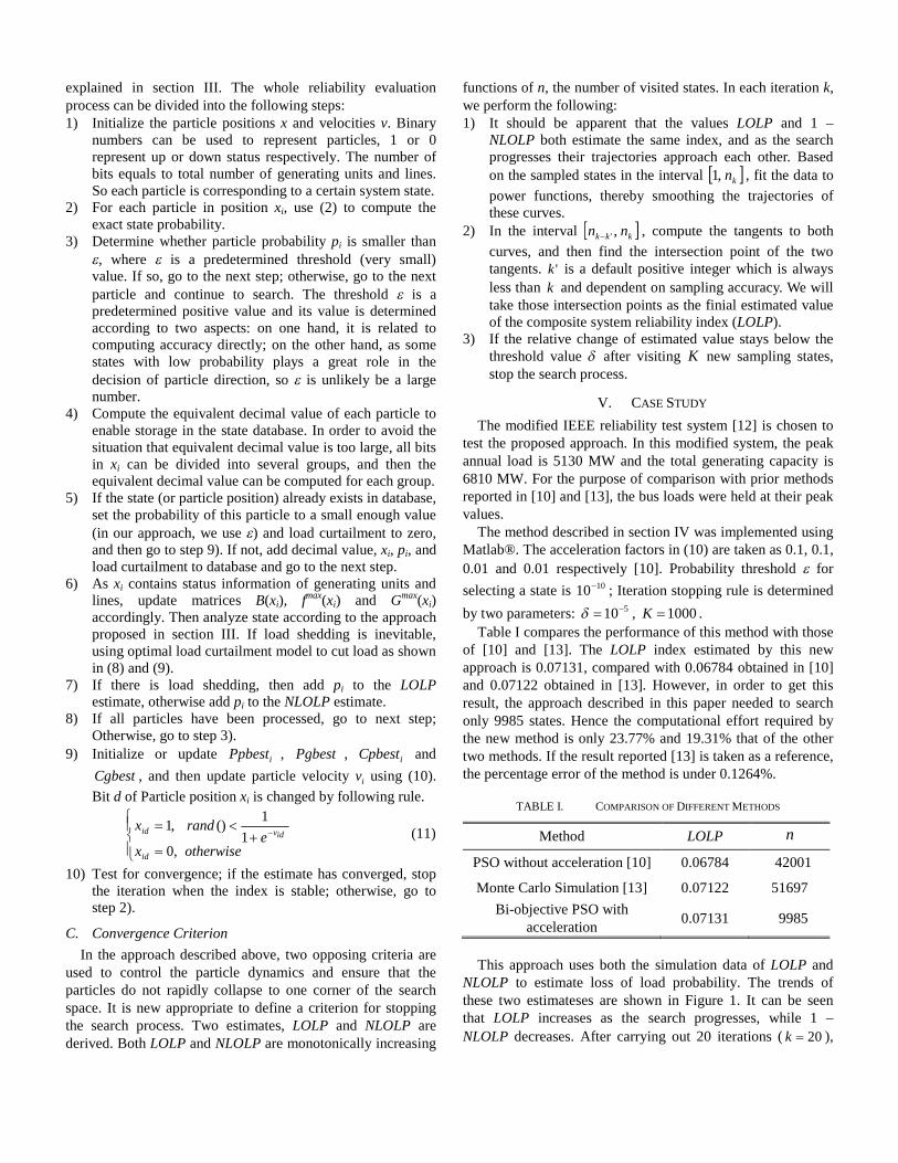
This approach uses both the simulation data of LOLP andNLOLP to estimate loss of load probability. The trends ofthese two estimateses are shown in Figure 1. It can be seenthat LOLP increases as the search progresses, while 1 –

NLOLP decreases. After carrying out 20 iterations ( 20k ),

we plot both fitting curves of LOLP and 1 – NLOLP using all

visited states at interval kkk nn ,' ( 10'k ). The intersection

points of tangents are indicated with black spots which areemployed to estimate loss of load probability.

From Figure 1, we can find three features of profile curve ofthe accelerated estimate from the intersection of the tangents:1) It fluctuates at the beginning, but later converges betterconvergence than any other two fitting curves (LOLP and 1 –NLOLP). In the first 9985 states visited, neither the LOLPcurve nor the 1 – NLOLP curve is close to the system LOLP,but the accelerated estimate reaches the system LOLP withnegligible error. 2) At convergence, the sum of probability ofstates which have not been visited is only 0.08258. Thisproves that bi-objective BPSO proposed has a strong ability inseeking out states that have effectively contribute to thesystem LOLP. 3) Due to the monotonicity of the two fittingcurves, sampling value of intersection point of tangents isalways between corresponding LOLP and 1 – NLOLP. So thisintersection point constitutes an effective accelerated estimate.

0 0.2 0.4 0.6 0.8 1 1.2 1.4 1.6 1.8 2

x 104

0

0.1

0.2

0.3

0.4

0.5

0.6

0.7

0.8

0.9

1

State Number

Pro

ba

bili

ty

LOLP Sampling Value

LOLP Fitting Curve

'1-NLOLP' Sampling Value

'1-NLOLP' Fitting Curve

Intersection Point of Tangents

Figure 1. Trajectories of successive estimates

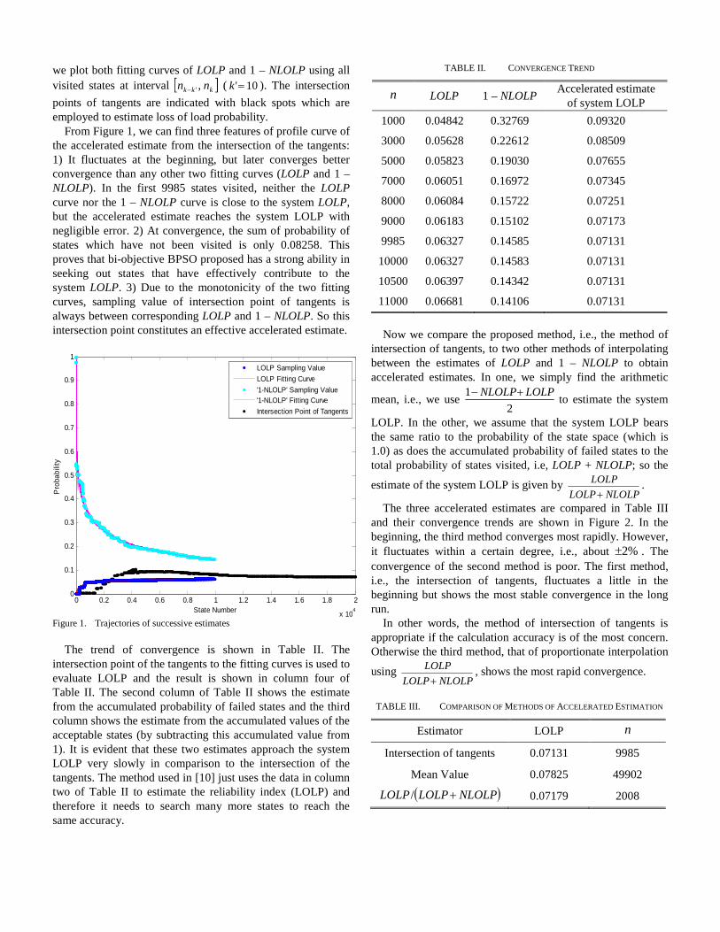
The trend of convergence is shown in Table II. Theintersection point of the tangents to the fitting curves is used toevaluate LOLP and the result is shown in column four ofTable II. The second column of Table II shows the estimatefrom the accumulated probability of failed states and the thirdcolumn shows the estimate from the accumulated values of theacceptable states (by subtracting this accumulated value from1). It is evident that these two estimates approach the systemLOLP very slowly in comparison to the intersection of thetangents. The method used in [10] just uses the data in columntwo of Table II to estimate the reliability index (LOLP) andtherefore it needs to search many more states to reach thesame accuracy.

TABLE II. CONVERGENCE TREND

n LOLP 1 – NLOLPAccelerated estimate

of system LOLP

1000 0.04842 0.32769 0.09320

3000 0.05628 0.22612 0.08509

5000 0.05823 0.19030 0.07655

7000 0.06051 0.16972 0.07345

8000 0.06084 0.15722 0.07251

9000 0.06183 0.15102 0.07173

9985 0.06327 0.14585 0.07131

10000 0.06327 0.14583 0.07131

10500 0.06397 0.14342 0.07131

11000 0.06681 0.14106 0.07131

Now we compare the proposed method, i.e., the method ofintersection of tangents, to two other methods of interpolatingbetween the estimates of LOLP and 1 – NLOLP to obtainaccelerated estimates. In one, we simply find the arithmetic

mean, i.e., we use2

1 LOLPNLOLPto estimate the system

LOLP. In the other, we assume that the system LOLP bearsthe same ratio to the probability of the state space (which is1.0) as does the accumulated probability of failed states to thetotal probability of states visited, i.e, LOLP + NLOLP; so the

estimate of the system LOLP is given byNLOLPLOLP

LOLP

.

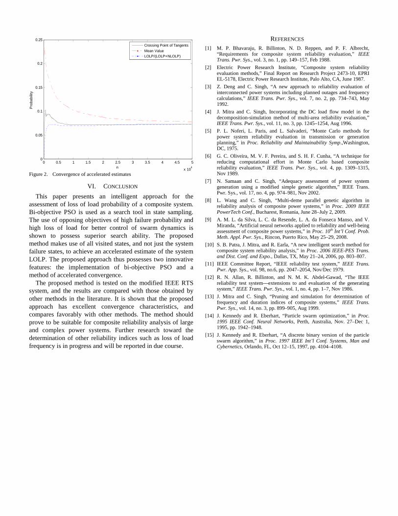
The three accelerated estimates are compared in Table IIIand their convergence trends are shown in Figure 2. In thebeginning, the third method converges most rapidly. However,

it fluctuates within a certain degree, i.e., about %2 . The

convergence of the second method is poor. The first method,i.e., the intersection of tangents, fluctuates a little in thebeginning but shows the most stable convergence in the longrun.

In other words, the method of intersection of tangents isappropriate if the calculation accuracy is of the most concern.Otherwise the third method, that of proportionate interpolation

usingNLOLPLOLP

LOLP

, shows the most rapid convergence.

TABLE III. COMPARISON OF METHODS OF ACCELERATED ESTIMATION

Estimator LOLP n

Intersection of tangents 0.07131 9985

Mean Value 0.07825 49902

NLOLPLOLPLOLP / 0.07179 2008

0 0.5 1 1.5 2 2.5 3 3.5 4 4.5 5

x 104

0

0.05

0.1

0.15

0.2

0.25

n

Pro

babili

ty

Crossing Point of Tangents

Mean Value

LOLP/(LOLP+NLOLP)

Figure 2. Convergence of accelerated estimates

VI. CONCLUSION

This paper presents an intelligent approach for theassessment of loss of load probability of a composite system.Bi-objective PSO is used as a search tool in state sampling.The use of opposing objectives of high failure probability andhigh loss of load for better control of swarm dynamics isshown to possess superior search ability. The proposedmethod makes use of all visited states, and not just the systemfailure states, to achieve an accelerated estimate of the systemLOLP. The proposed approach thus possesses two innovativefeatures: the implementation of bi-objective PSO and amethod of accelerated convergence.

The proposed method is tested on the modified IEEE RTSsystem, and the results are compared with those obtained byother methods in the literature. It is shown that the proposedapproach has excellent convergence characteristics, andcompares favorably with other methods. The method shouldprove to be suitable for composite reliability analysis of largeand complex power systems. Further research toward thedetermination of other reliability indices such as loss of loadfrequency is in progress and will be reported in due course.

REFERENCES

[1] M. P. Bhavaraju, R. Billinton, N. D. Reppen, and P. F. Albrecht,“Requirements for composite system reliability evaluation,” IEEETrans. Pwr. Sys., vol. 3, no. 1, pp. 149–157, Feb 1988.

[2] Electric Power Research Institute, “Composite system reliabilityevaluation methods,” Final Report on Research Project 2473-10, EPRIEL-5178, Electric Power Research Institute, Palo Alto, CA, June 1987.

[3] Z. Deng and C. Singh, “A new approach to reliability evaluation ofinterconnected power systems including planned outages and frequencycalculations,” IEEE Trans. Pwr. Sys., vol. 7, no. 2, pp. 734–743, May1992.

[4] J. Mitra and C. Singh, Incorporating the DC load flow model in thedecomposition-simulation method of multi-area reliability evaluation,”IEEE Trans. Pwr. Sys., vol. 11, no. 3, pp. 1245–1254, Aug 1996.

[5] P. L. Noferi, L. Paris, and L. Salvaderi, “Monte Carlo methods forpower system reliability evaluation in transmission or generationplanning,” in Proc. Reliability and Maintainability Symp.,Washington,DC, 1975.

[6] G. C. Oliveira, M. V. F. Pereira, and S. H. F. Cunha, “A technique forreducing computational effort in Monte Carlo based compositereliability evaluation,” IEEE Trans. Pwr. Sys., vol. 4, pp. 1309–1315,Nov 1989.

[7] N. Samaan and C. Singh, “Adequacy assessment of power systemgeneration using a modified simple genetic algorithm,” IEEE Trans.Pwr. Sys., vol. 17, no. 4, pp. 974–981, Nov 2002.

[8] L. Wang and C. Singh, “Multi-deme parallel genetic algorithm inreliability analysis of composite power systems,” in Proc. 2009 IEEEPowerTech Conf., Bucharest, Romania, June 28–July 2, 2009.

[9] A. M. L. da Silva, L. C. da Resende, L. A. da Fonseca Manso, and V.Miranda, “Artificial neural networks applied to reliability and well-beingassessment of composite power systems,” in Proc. 10th Int’l Conf. Prob.Meth. Appl. Pwr. Sys., Rincon, Puerto Rico, May 25–29, 2008.

[10] S. B. Patra, J. Mitra, and R. Earla, “A new intelligent search method forcomposite system reliability analysis,” in Proc. 2006 IEEE-PES Trans.and Dist. Conf. and Expo., Dallas, TX, May 21–24, 2006, pp. 803–807.

[11] IEEE Committee Report, “IEEE reliability test system,” IEEE Trans.Pwr. App. Sys., vol. 98, no.6, pp. 2047–2054, Nov/Dec 1979.

[12] R. N. Allan, R. Billinton, and N. M. K. Abdel-Gawad, “The IEEEreliability test system—extensions to and evaluation of the generatingsystem,” IEEE Trans. Pwr. Sys., vol. 1, no. 4, pp. 1–7, Nov 1986.

[13] J. Mitra and C. Singh, “Pruning and simulation for determination offrequency and duration indices of composite systems,” IEEE Trans.Pwr. Sys., vol. 14, no. 3, pp. 899–905, Aug 1999.

[14] J. Kennedy and R. Eberhart, “Particle swarm optimization,” in Proc.1995 IEEE Conf. Neural Networks, Perth, Australia, Nov. 27–Dec 1,1995, pp. 1942–1948.

[15] J. Kennedy and R. Eberhart, “A discrete binary version of the particleswarm algorithm,” in Proc. 1997 IEEE Int’l Conf. Systems, Man andCybernetics, Orlando, FL, Oct 12–15, 1997, pp. 4104–4108.