Complexity Results and Algorithms for Argumentation · in diverse applications including legal reasoning, E-Democracy tools, medical applications and many more. An integral part of

Complexity Results andAlgorithms for Argumentation

Dung’s Frameworks and Beyond

DISSERTATION

submitted in partial fulfillment of the requirements for the degree of

Doktor der technischen Wissenschaften

by

Johannes Peter WallnerRegistration Number 0327240

to the Faculty of Informaticsat the Vienna University of Technology

Advisor: Associate Prof. Dr. Stefan WoltranAdvisor: Assistant Prof. Georg Weissenbacher, D.Phil.Assistance: Dr. Wolfgang Dvorák

The dissertation has been reviewed by:

(Associate Prof. Dr. StefanWoltran)

(Prof. Gerhard Brewka)

Wien, 03.04.2014(Johannes Peter Wallner)

Technische Universität WienA-1040 Wien � Karlsplatz 13 � Tel. +43-1-58801-0 � www.tuwien.ac.at

Die approbierte Originalversion dieser Dissertation ist in der Hauptbibliothek der Technischen Universität Wien aufgestellt und zugänglich. http://www.ub.tuwien.ac.at

The approved original version of this thesis is available at the main library of the Vienna University of Technology.

http://www.ub.tuwien.ac.at/eng

Erklärung zur Verfassung der Arbeit

Johannes Peter WallnerFavoritenstraße 9–11, 1040 Wien

Hiermit erkläre ich, dass ich diese Arbeit selbständig verfasst habe, dass ich die verwen-deten Quellen und Hilfsmittel vollständig angegeben habe und dass ich die Stellen der Arbeit- einschließlich Tabellen, Karten und Abbildungen -, die anderen Werken oder dem Internetim Wortlaut oder dem Sinn nach entnommen sind, auf jeden Fall unter Angabe der Quelle alsEntlehnung kenntlich gemacht habe.

(Ort, Datum) (Unterschrift Verfasser)

i

Acknowledgements

Every work builds upon the support of many people. This is also the case with this thesis. FirstI would like to thank my family, my parents Ludmilla and Wolfgang who supported me in allsituations in life (in addition to giving me one in the first place). Thanks also to my brotherMatthias, who told me to give the study of computer science a try. Further I want to thankMatthias’ wife Sabine and in particular their son Tobias for being an inspiration.

During my work I had the opportunity to have a lot of splendid colleagues. I enjoyed thefruitful discussions, chats and amicable atmosphere here at the Institute of Information Sys-tems. I cannot give here everyone enough words for the support they gave me, but at least Iwant to list them in a (probably) incomplete and unsorted set. I want to thank {Günther Char-wat, Matti Järvisalo, Friedrich Slivovsky, Srdjan Vesic, Markus Pichlmair, Stefan Ellmauthaler,Florian Lonsing, Andreas Pfandler, Christof Redl, Sylwia Polberg, Reinhard Pichler, Toni Pis-jak, Hannes Strass, Ringo Baumann, Georg Weissenbacher, Magdalena Widl, Frank Loebe,Thomas Krennwallner, Lara Spendier, Emanuel Sallinger, Bernhard Bliem, Martin Lackner,Axel Polleres, Martin Baláž, Jozef Frtús, Dragan Doder, Nysret Musliu, Giselle Reis, DariaStepanova, Thomas Linsbichler, Paolo Baldi, Martin Kronegger}.

There are some people without this work and indeed my whole job at the institute, would nothave been fruitful and even more probably would have been actually impossible. As in movies,I give special thanks to Gerhard Brewka, for having me as a guest in Leipzig, I enjoyed the stayand learnt a lot there. Further I thank my two “seniors”, Sarah Gaggl and Wolfgang Dvorák,who particularly supported me in our project and gave me a lot of insights into academic life.A very special thanks goes to Stefan Woltran. Not only because he is my main supervisor, butbecause he gave me invaluable knowledge, support and understanding. I count myself lucky tobe your student.

During my studies I have been given the opportunity to participate in the doctoral programme“Mathematical Logic in Computer Science”. I am thankful for the beneficial atmosphere and theinterdisciplinary workshops within this programme, which was funded by the Vienna Universityof Technology. Last, but not least, I thank the Vienna Science and Technology Fund (WWTF),Deutsche Forschungsgemeinschaft (DFG) and the Austrian Science Fund (FWF) for funding thefollowing research projects I participated in: ICT08-028, ICT12-015 and I1102.

iii

Abstract

In the last couple of decades argumentation emerged as an important topic in Artificial Intelli-gence (AI). Having its origin in philosophy, law and formal logic, argumentation in combinationwith computer science has developed into various formal models, which nowadays are foundin diverse applications including legal reasoning, E-Democracy tools, medical applications andmany more. An integral part of many formal argumentation theories within AI is a certain notionof abstraction. Hereby the actual contents of arguments are disregarded, but only the relation be-tween them is used for reasoning purposes. One very influential formal model for representingdiscourses abstractly are Dung’s argumentation frameworks (AFs). AFs can simply be repre-sented as directed graphs. The vertices correspond to abstract arguments and directed edges areinterpreted as an attack relation for countering arguments. Many variants and generalizations ofAFs have been devised, with abstract dialectical frameworks (ADFs) among the most generalones. ADFs are even more abstract than AFs: the relation between arguments is not fixed to theconcept attack, but is specified via so-called acceptance conditions, describing the relationshipvia Boolean functions.

The main computational challenge for AFs and ADFs is to compute jointly acceptable setsof arguments. Several criteria, termed semantics, have been proposed for accepting arguments.Applications of AFs or ADFs unfortunately face the harsh reality that almost all reasoning tasksdefined for the frameworks are intractable. Decision problems for AFs can even be hard forthe second level of the polynomial hierarchy. ADFs generalize AFs and thus are at least ascomputationally complex, but exact complexity bounds of many ADF problems are lacking inthe literature.

There have been some proposals how to implement reasoning tasks on AFs. Roughly thesecan be classified into reduction and direct approaches. The former approach solves the prob-lem at hand by translation to another one, for which sophisticated solvers exist. However, atthe start of this thesis, reduction approaches for argumentation were purely monolithic. Mono-lithic reduction approaches result into a single encoding and hardly incorporate domain-specificoptimizations for more efficient computation. Direct approaches exploit structural or semanti-cal properties of AFs for efficiency but must typically devise and implement an algorithm fromscratch, including the highly consuming task of engineering solutions on a very deep algorithmiclevel e.g. the development of suitable data structures.

In this thesis we provide three major contributions to the state of the art in abstract argumen-tation. First, we develop a novel hybrid approach that combines strengths of reduction and directapproaches. Our method reduces the problem at hand to iterative satisfiability (SAT) solving,

v

i.e. a sequence of calls to a SAT-solver. Due to hardness for the second level of the polyno-mial hierarchy, we cannot avoid exponentially many SAT calls in the worst case. However, byexploiting inherent parameters of AFs, we provide a bound on the number of calls. Utilizingmodern SAT technology to an even greater extent, we also employ more expressive variants ofthe SAT problem. It turns out that minimal correction sets (MCSes) and backbones of Booleanformulae are very well suited for our tasks. Like the iterative SAT algorithms, our algorithmsbased upon MCSes and backbones are hybrid approaches as well. Yet they are closer to mono-lithic reduction approaches and offer the benefit of requiring even less engineering effort andproviding more declarativeness.

Our second major contribution is to generalize our algorithms to ADFs. For doing so wefirst considerably extend ADF theory and provide a thorough complexity analysis for ADFs.Our results show that the reasoning tasks for ADFs are one step up in the polynomial hierarchycompared to their counterparts on AFs. Even though problems on ADFs suffer from hardnessup to the third level of the polynomial hierarchy, our analysis shows that bipolar ADFs (BADFs)are not affected by this complexity jump. BADFs restrict the relations between arguments to beeither of an attacking or supporting nature, but still offer a variety of interesting relations.

Finally our third contribution is an empirical evaluation of implementations of our algo-rithms. Our novel algorithms outperform existing state-of-the-art systems for abstract argumen-tation. These results show that our hybrid approaches are indeed promising and that the providedproof-of-concept implementations can pave the way for applications for handling problems ofincreasing size and complexity.

Kurzfassung

In den letzten Jahrzehnten hat sich die Argumentationstheorie als wichtiges Teilgebiet der Kün-stlichen Intelligenz (KI) etabliert. Die vielfältigen Wurzeln dieses jungen Gebietes liegen sowohlin der Philosophie, in den Rechtswissenschaften, als auch in der formalen Logik. Unterstütztdurch die Computerwissenschaften ergaben sich aus dieser Theorie ebenso vielfältige Anwen-dungen, unter anderem für rechtliche Beweisführung, Medizin und E-Democracy. Als zentralerAspekt, der in vielen Formalisierungen von Argumentation auftaucht, erweist sich eine gewisseForm von Abstraktion. Meist wird in einem solchen Abstraktionsprozess von konkreten Inhaltenvon Argumenten Abstand genommen und nur deren logische Relation betrachtet. Ein einflussre-iches formales Model für die abstrakte Repräsentation von Diskursen sind die so genanntenArgumentation Frameworks (AFs), entwickelt von Phan Minh Dung. In diesen AFs werden Ar-gumente einfach als abstrakte Knoten in einem Graph dargestellt. Gerichtete Kanten repräsen-tieren wiederum die Relation zwischen Argumenten, welche in AFs als Angriff interpretiertwird. Beispielsweise kann ein attackierendes Argument als Gegenargument gesehen werden. Inder Literatur wurden diverse Aspekte von AFs verallgemeinert, oder erweitert. Ein besondersgenereller Vertreter dieser formalen Modelle sind die Abstract Dialectical Frameworks (ADFs).ADFs sind noch abstrakter als AFs, denn die Relation in ADFs beschränkt sich nicht auf Attack-en, sondern kann mittels so genannter Akzeptanzbedingungen frei spezifiziert werden. DieseBedingungen werden mittels boolescher Formeln modelliert.

Die logischen Semantiken dieser Argumentationsstrukturen bestehen aus verschiedenen Kri-terien zur Akzeptanz von Argumenten. Die automatische Berechnung von Mengen von Argu-menten die gemeinsam akzeptiert werden können ist eine der wichtigsten Aufgaben auf AFs undADFs. Allerdings haben praktisch alle solche Problemstellungen eine hohe Berechnungskom-plexität. Manche Probleme auf AFs sind sogar hart für die zweite Stufe der polynomiellen Hi-erarchie. AFs sind Spezialfälle von ADFs, daher sind ADFs auch mindestens so komplex wasdie Berechnung der Semantiken angeht. Eine genaue Analyse der Komplexitätsschranken warjedoch offen für ADFs.

Um diese Aufgaben dennoch zu bewältigen sind einige Algorithmen für AFs entwickeltworden. Man kann diese in zwei Richtungen klassifizieren. Die erste Richtung beschäftigt sichmit Reduktionen oder auch Übersetzungen. Dabei wird das Ursprungsproblem in ein andereskodiert, für das performante Systeme existieren. Zu Beginn der Arbeiten an dieser Dissertationwaren Reduktionen allerdings von rein monolithischer Natur. Das heißt, dass diese Reduktio-nen das Ursprungsproblem in eine einzelne Kodierung übersetzen. Zudem wurden in diesenÜbersetzungen kaum Optimierungen berücksichtigt. Die zweite Richtung besteht aus direktenMethoden. Diese können leichter strukturelle oder semantische Eigenschaften von AFs nutzen

vii

um effizient Lösungen zu berechnen. Allerdings müssen hierfür Algorithmen von Grund auf neuimplementiert werden. Das beinhaltet auch die zeitintensive Aufgabe geeignete Datenstrukturenund andere technische Details auszuarbeiten.

Unser Beitrag zum wissenschaftlichen Stand der Technik in der Argumentationstheorie lässtsich in drei Bereiche gliedern. Erstens entwickeln wir hybride Ansätze, welche die Stärken vonReduktionen und direkten Methoden vereinen. Dabei reduzieren wir die Problemstellungen aufeine Folge von booleschen Erfüllbarkeitsproblemen (SAT). Bei Problemen die hart für die zweiteStufe der polynomiellen Hierarchie sind, lässt es sich, unter komplexitätstheoretischen Annah-men, nicht vermeiden, dass wir im schlimmsten Fall eine exponentielle Anzahl solcher Teil-probleme lösen müssen. Durch Verwendung von inhärenten Parametern von AFs können wirdiese Anzahl jedoch beschränken. Zusätzlich zu dem klassischen SAT Problem, zeigen wir, dasssich Probleme in der Argumentation natürlicherweise auf Erweiterungen des SAT Problems re-duzieren lassen. Konkret nutzen wir minimal correction sets (MCSes) und backbones von boo-leschen Formeln hierfür. Reduktionen zu diesen sind ebenfalls hybrid, allerdings näher zu striktmonolithischen Ansätzen und auch deklarativer als die anderen hybriden Methoden.

Als zweites Ergebnis unserer Arbeit stellen wir Verallgemeinerungen unserer hybriden An-sätze für ADFs vor. Hierfür erweitern wir zuerst die theoretische Basis und zeigen wesentlicheKomplexitätsresultate von ADFs. Es stellt sich heraus, dass Entscheidungsprobleme von ADFsim Allgemeinen eine um eine Stufe höhere Komplexität aufweisen als die jeweiligen Problemeauf AFs. Trotz der Tatsache, dass damit manche Probleme auf ADFs hart für die dritte Stufe derpolynomiellen Hierarchie sind, können wir zeigen, dass eine wichtige Teilklasse von ADFs, dieso genannten bipolaren ADFs (BADFs), nicht von der erhöhten Komplexität betroffen sind.

Unser dritter Beitrag besteht aus Implementierungen unserer Methoden für AFs und derenexperimentelle Evaluierung. Wir zeigen, dass unsere Implementierungen performanter als an-dere Systeme im Bereich der Argumentationstheorie sind. Diese Resultate deuten daraufhin,dass unsere hybriden Ansätze gut geeignet sind um die schwierigen Aufgaben, die in dieserTheorie vorkommen, zu bewältigen. Insbesondere können unsere prototypischen Softwareim-plementierungen den Weg für Anwendungen, mit noch größeren Strukturen umzugehen, ebnen.

Contents

List of Figures 1

List of Tables 2

List of Algorithms 3

1 Introduction 51.1 Argumentation Theory in AI . . . . . . . . . . . . . . . . . . . . . . . . . . . 51.2 Main Contributions . . . . . . . . . . . . . . . . . . . . . . . . . . . . . . . . 81.3 Structure of the Thesis . . . . . . . . . . . . . . . . . . . . . . . . . . . . . . 101.4 Publications . . . . . . . . . . . . . . . . . . . . . . . . . . . . . . . . . . . . 11

2 Background 132.1 General Definitions and Notation . . . . . . . . . . . . . . . . . . . . . . . . . 132.2 Propositional Logic . . . . . . . . . . . . . . . . . . . . . . . . . . . . . . . . 14

2.2.1 Propositional Formulae . . . . . . . . . . . . . . . . . . . . . . . . . . 142.2.2 Quantified Boolean Formulae . . . . . . . . . . . . . . . . . . . . . . 162.2.3 Normal Forms . . . . . . . . . . . . . . . . . . . . . . . . . . . . . . 182.2.4 Semantics . . . . . . . . . . . . . . . . . . . . . . . . . . . . . . . . . 19

2.3 Argumentation in Artificial Intelligence . . . . . . . . . . . . . . . . . . . . . 242.3.1 Argumentation Frameworks . . . . . . . . . . . . . . . . . . . . . . . 242.3.2 Semantics of Argumentation Frameworks . . . . . . . . . . . . . . . . 262.3.3 Abstract Dialectical Frameworks . . . . . . . . . . . . . . . . . . . . . 332.3.4 Semantics of Abstract Dialectical Frameworks . . . . . . . . . . . . . 36

2.4 Computational Complexity . . . . . . . . . . . . . . . . . . . . . . . . . . . . 442.4.1 Basics . . . . . . . . . . . . . . . . . . . . . . . . . . . . . . . . . . . 442.4.2 Complexity of Abstract Argumentation: State of the Art . . . . . . . . 48

3 Advanced Algorithms for Argumentation Frameworks 533.1 SAT Solving . . . . . . . . . . . . . . . . . . . . . . . . . . . . . . . . . . . . 553.2 Classes of Argumentation Frameworks . . . . . . . . . . . . . . . . . . . . . . 583.3 Search Algorithms . . . . . . . . . . . . . . . . . . . . . . . . . . . . . . . . 60

3.3.1 Generic Algorithm . . . . . . . . . . . . . . . . . . . . . . . . . . . . 613.3.2 Search Algorithms for Preferred Semantics . . . . . . . . . . . . . . . 65

ix

3.3.3 Search Algorithms for Semi-stable and Stage Semantics . . . . . . . . 703.3.4 Variants for Query Based Reasoning . . . . . . . . . . . . . . . . . . . 72

3.4 Utilizing Minimal Correction Sets and Backbones . . . . . . . . . . . . . . . . 783.4.1 SAT Extensions . . . . . . . . . . . . . . . . . . . . . . . . . . . . . . 783.4.2 MCS Algorithm for Semi-stable and Stage Semantics . . . . . . . . . . 803.4.3 MCS Algorithm for Eager and Stage-ideal Semantics . . . . . . . . . . 833.4.4 Backbone Algorithm for Ideal Semantics . . . . . . . . . . . . . . . . 84

3.5 Summary . . . . . . . . . . . . . . . . . . . . . . . . . . . . . . . . . . . . . 84

4 Abstract Dialectical Frameworks: Novel Complexity Results and Algorithms 874.1 Complexity Analysis of ADFs . . . . . . . . . . . . . . . . . . . . . . . . . . 88

4.1.1 Complexity Analysis of General ADFs . . . . . . . . . . . . . . . . . 88Computational Complexity of the Grounded Semantics . . . . . . . . . 88Computational Complexity of the Admissible Semantics . . . . . . . . 96Computational Complexity of the Preferred Semantics . . . . . . . . . 98

4.1.2 Complexity Analysis of Bipolar ADFs . . . . . . . . . . . . . . . . . . 1024.2 Algorithms for ADFs . . . . . . . . . . . . . . . . . . . . . . . . . . . . . . . 106

4.2.1 Search Algorithm for Preferred Semantics . . . . . . . . . . . . . . . . 1064.2.2 Backbone Algorithm for Grounded Semantics . . . . . . . . . . . . . . 107

4.3 Summary . . . . . . . . . . . . . . . . . . . . . . . . . . . . . . . . . . . . . 108

5 Implementation and Empirical Evaluation 1095.1 System Description . . . . . . . . . . . . . . . . . . . . . . . . . . . . . . . . 109

5.1.1 CEGARTIX . . . . . . . . . . . . . . . . . . . . . . . . . . . . . . . . 1105.1.2 SAT Extension based Algorithms . . . . . . . . . . . . . . . . . . . . 111

5.2 Experiments . . . . . . . . . . . . . . . . . . . . . . . . . . . . . . . . . . . . 1135.2.1 Test Setup . . . . . . . . . . . . . . . . . . . . . . . . . . . . . . . . . 1135.2.2 Evaluation of CEGARTIX . . . . . . . . . . . . . . . . . . . . . . . . 1145.2.3 Impact of Base Semantics and Shortcuts within CEGARTIX . . . . . . 1185.2.4 Effect of the Choice of SAT Solver within CEGARTIX . . . . . . . . . 1205.2.5 Evaluation of SAT Extensions based Algorithms . . . . . . . . . . . . 121

5.3 Summary . . . . . . . . . . . . . . . . . . . . . . . . . . . . . . . . . . . . . 123

6 Discussion 1256.1 Summary . . . . . . . . . . . . . . . . . . . . . . . . . . . . . . . . . . . . . 1256.2 Related Work . . . . . . . . . . . . . . . . . . . . . . . . . . . . . . . . . . . 1276.3 Future Work . . . . . . . . . . . . . . . . . . . . . . . . . . . . . . . . . . . . 134

Bibliography 137

A Algorithms 153

B Curriculum Vitae 157

x

List of Figures

1.1 Argumentation process . . . . . . . . . . . . . . . . . . . . . . . . . . . . . . . . 61.2 Frameworks for argumentation . . . . . . . . . . . . . . . . . . . . . . . . . . . . 7

2.1 Subformula substitution example . . . . . . . . . . . . . . . . . . . . . . . . . . . 162.2 Truth tables for classical two–valued logic . . . . . . . . . . . . . . . . . . . . . . 212.3 Truth table for the formula a ∧ (b ∨ ¬c) . . . . . . . . . . . . . . . . . . . . . . . 212.4 Truth tables for strong three–valued logic of Kleene . . . . . . . . . . . . . . . . . 242.5 Example argumentation framework F . . . . . . . . . . . . . . . . . . . . . . . . 252.6 Condensation of AF from Example 2.3.1 . . . . . . . . . . . . . . . . . . . . . . . 262.7 Argumentation framework F ′ containing an isolated self-attacking argument . . . . 302.8 Relation between AF semantics . . . . . . . . . . . . . . . . . . . . . . . . . . . . 322.9 ADF with different link types . . . . . . . . . . . . . . . . . . . . . . . . . . . . . 362.10 Bipolar ADF . . . . . . . . . . . . . . . . . . . . . . . . . . . . . . . . . . . . . 372.11 Meet-semilattice of three-valued interpretations . . . . . . . . . . . . . . . . . . . 382.12 Relation between ADF semantics . . . . . . . . . . . . . . . . . . . . . . . . . . . 432.13 Example AF conversion to ADF . . . . . . . . . . . . . . . . . . . . . . . . . . . 442.14 Relation between complexity classes . . . . . . . . . . . . . . . . . . . . . . . . . 48

3.1 Basic workflow for the algorithms based on iterative SAT procedures . . . . . . . . 543.2 Example implication graph . . . . . . . . . . . . . . . . . . . . . . . . . . . . . . 573.3 Example argumentation framework F . . . . . . . . . . . . . . . . . . . . . . . . 603.4 Illustration of Algorithm 1 . . . . . . . . . . . . . . . . . . . . . . . . . . . . . . 633.5 Difference of complete and admissible base semantics for Algorithm 6 . . . . . . . 77

4.1 Constructed ADF for hardness proof of Proposition 4.1.11. . . . . . . . . . . . . . 984.2 Constructed ADF for hardness proof of Lemma 4.1.13. . . . . . . . . . . . . . . . 994.3 Constructed ADF for hardness proof of Theorem 4.1.17. . . . . . . . . . . . . . . 100

5.1 Examples of grid-structured AFs . . . . . . . . . . . . . . . . . . . . . . . . . . . 1145.2 Performance comparison of ASPARTIX and CEGARTIX for skeptical reasoning . 1165.3 Performance comparison of ASPARTIX and CEGARTIX for credulous reasoning . 1175.4 Effect of choice of base semantics for CEGARTIX for semi-stable reasoning . . . . 1185.5 Effect of choice of base semantics for CEGARTIX for preferred reasoning . . . . . 1195.6 Effect of choice of SAT-solver within CEGARTIX . . . . . . . . . . . . . . . . . . 120

1

5.7 Mean running time for CEGARTIX and the MCS-based algorithm. . . . . . . . . . 1215.8 Mean running time for computing the ideal respectively eager extension. . . . . . . 122

6.1 Recursive calls of Algorithm 9 from [129] . . . . . . . . . . . . . . . . . . . . . . 1306.2 Tree decomposition of AF from Example 2.5 with width 2 . . . . . . . . . . . . . 131

List of Tables

2.1 Evaluation criteria for AF semantics . . . . . . . . . . . . . . . . . . . . . . . . . 332.2 Interpretations of the ADF from Example 2.3.7 . . . . . . . . . . . . . . . . . . . 412.3 Interpretations of the ADF from Example 2.3.12 . . . . . . . . . . . . . . . . . . . 412.4 Transition function of the deterministic Turing machine from Example 2.4.1 . . . . 462.5 Computational complexity of propositional logic . . . . . . . . . . . . . . . . . . 492.6 Computational complexity of reasoning in AFs . . . . . . . . . . . . . . . . . . . 50

3.1 CDCL example . . . . . . . . . . . . . . . . . . . . . . . . . . . . . . . . . . . . 573.2 Algorithms overview . . . . . . . . . . . . . . . . . . . . . . . . . . . . . . . . . 85

4.1 Values of Igrd(D) for accepted and rejected arguments . . . . . . . . . . . . . . . . 934.2 Values of Igrd(D) for undecided arguments . . . . . . . . . . . . . . . . . . . . . . 934.3 Example ADF illustrating use of duplicates in reduction to Boolean logic for grounded

semantics . . . . . . . . . . . . . . . . . . . . . . . . . . . . . . . . . . . . . . . 964.4 Result of canonD(I, s, v) = J for a BADF D . . . . . . . . . . . . . . . . . . . . 1034.5 Computational complexity of reasoning in ADFs and BADFs with known link types 108

5.1 Timeouts encountered with ASPARTIX on medium-sized random/grid AFs . . . . 1155.2 Number of solved instances for CEGARTIX and the MCS-based algorithm. . . . . 1215.3 Overview of implementations . . . . . . . . . . . . . . . . . . . . . . . . . . . . . 1235.4 Supported reasoning tasks and solver . . . . . . . . . . . . . . . . . . . . . . . . . 124

2

List of Algorithms

1 Generic(F, a,M, σ, σ′,≺) . . . . . . . . . . . . . . . . . . . . . . . . . . . . 632 Preferred(F, a,M, σ′) . . . . . . . . . . . . . . . . . . . . . . . . . . . . . . . 663 Preferred-SAT(F, a,M, σ′) . . . . . . . . . . . . . . . . . . . . . . . . . . . . 694 Semi-stable(F, a,M, σ′) . . . . . . . . . . . . . . . . . . . . . . . . . . . . . 705 Semi-stable-SAT(F, a,M, σ′) . . . . . . . . . . . . . . . . . . . . . . . . . . 716 Decide(F, a,M, σ, σ′) . . . . . . . . . . . . . . . . . . . . . . . . . . . . . . 747 Shortcuts(F, a, co-Skept, prf , σ′) . . . . . . . . . . . . . . . . . . . . . . . . 758 Shortcuts(F, a,M, σ, σ′) . . . . . . . . . . . . . . . . . . . . . . . . . . . . . 769 MCS(φ) (simplified version of [115]) . . . . . . . . . . . . . . . . . . . . . . 7910 Probing(φ) (adapted from [122]) . . . . . . . . . . . . . . . . . . . . . . . . . 8011 MCS-AllSkeptsem(F ) . . . . . . . . . . . . . . . . . . . . . . . . . . . . . . . 8212 MCS-Eager(F ) . . . . . . . . . . . . . . . . . . . . . . . . . . . . . . . . . . 8313 Ideal(F ) [62] . . . . . . . . . . . . . . . . . . . . . . . . . . . . . . . . . . . 8414 Preferred-ADF(D, a,M) . . . . . . . . . . . . . . . . . . . . . . . . . . . . . 10715 Stage(F, a,M) . . . . . . . . . . . . . . . . . . . . . . . . . . . . . . . . . . 15316 Stage-SAT(F, a,M) . . . . . . . . . . . . . . . . . . . . . . . . . . . . . . . 15417 MCS-AllSkeptstg(F ) . . . . . . . . . . . . . . . . . . . . . . . . . . . . . . . 15418 MCS-Stage-ideal(F ) . . . . . . . . . . . . . . . . . . . . . . . . . . . . . . . 155

3

CHAPTER 1Introduction

1.1 Argumentation Theory in AI

Imagine you present your vision to an audience. Some listeners might be curious about yourspeech and excited about everything you say. Some others might be skeptical about your ideasand remain distanced. An important topic deserves to be heard and fairly judged in any case.What does one do in this circumstance? You try to convince the audience of the importance ofyour vision and give persuading arguments. Persuasion has many forms. Aristotle distinguishedthree modes of persuasion: appealing to the presenter’s authority or honesty (ethos), to theaudience’s emotions (pathos) or to logic (logos). We focus here on argumentation by appealingto logic. Arguing is so natural to all of us that we do it all the time. Argumentation is part ofour daily lives when we discuss projects with colleagues, talk to partners about deciding whereto go for holiday, or try to persuade parents to watch a certain kind of movie. To our mind thefollowing citation succinctly summarizes the most important aspects of argumentation theory.

“In its classical treatment within philosophy, the study of argumentation may,informally, be considered as concerned with how assertions are proposed, dis-cussed, and resolved in the context of issues upon which several diverging opinionsmay be held.” Bench-Capon and Dunne [18]

In the last couple of decades argumentation emerged as a distinct field within Artificial In-telligence (AI) from considerations in philosophy, law and formal logic, constituting nowadaysan important subfield of AI [18, 22, 139]. A natural question is how argumentation in AI differsfrom classical logic? Bench-Capon and Dunne [18] argue as follows. In logic one proves state-ments. If a proof exists then the statement is not refutable. In contrast, the aim of arguments is topersuade, not to be formally proven. Moreover, arguments are defeasible. Thus, what made anargument convincing, might not be convincing anymore in the light of new information. Argu-mentation therefore can be considered as non-monotonic, that is, it might be necessary to retract

5

knowledge base

a?b!

c!

constructabstract model

d e

cb

a

evaluateacceptability

d e

cb

a

draw conclusions

b and e

Figure 1.1: Argumentation process

conclusions. Classical logic on the other hand is a monotonic formalism. What is proven correctonce, remains correct.

Although a formal mathematical proof of an argument is typically not possible, we stillwould like to assess whether a certain argumentation is reasonable or persuasive. With the ev-eryday examples one can maybe live with less reasonable choices, but there are many areaswhere a more strict assessment is necessary. It would be disastrous to consider arbitrary argu-ments in court to be valid or persuasive. Physicians discussing medical treatment should basetheir opinions on facts and scientific theory. Indeed in science itself one has to argue why someconclusion should be considered scientific and others not [111].

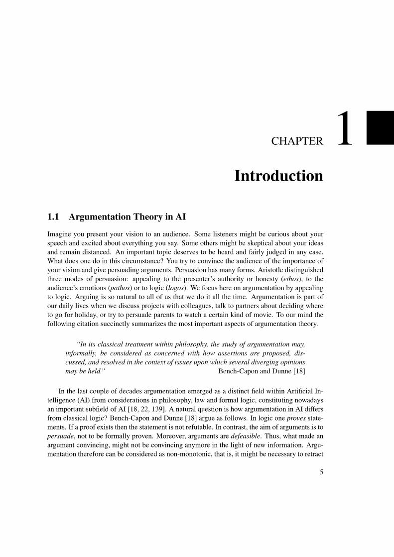
Automated reasoning is one of the main aspects of AI and argumentation provides a par-ticular challenge due to its non-monotonic derivations. Nevertheless, argumentation has foundits way into a variety of applications, such as in legal reasoning [17, 19], decision support sys-tems [1], E-Democracy tools [43, 44], E-Health tools [150], medical applications [95, 138],multi-agent systems [125], and more. An integral concept many formal argumentation theoriesand systems share is a certain notion of abstraction. Embedded in a larger workflow or argu-mentation process [40], formal models of argumentation represent arguments in an abstract way.Briefly put, in the argumentation process we assume a given knowledge base, which holds di-verging opinions of some sort. From this we construct an abstract representation of the relevantarguments for our current discourse and model their relations. Typically in this representationone abstracts away from the internal structure of the arguments [137]. Several formal models forthe abstract representation have been developed [33]. In the third step we evaluate the arguments.Evaluation in this context often refers to the act of finding sets of jointly acceptable arguments.Criteria for jointly accepting arguments are called semantics of the formal models. Finally wedraw conclusions from the accepted arguments. For instance an abstract argument may stand fora propositional logic formula [23]. Logically entailed formulae of accepted arguments are thenfurther conclusions. This process is outlined in Figure 1.1.

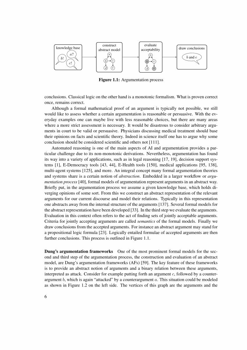
Dung’s argumentation frameworks One of the most prominent formal models for the sec-ond and third step of the argumentation process, the construction and evaluation of an abstractmodel, are Dung’s argumentation frameworks (AFs) [59]. The key feature of these frameworksis to provide an abstract notion of arguments and a binary relation between these arguments,interpreted as attack. Consider for example putting forth an argument c, followed by a counter-argument b, which is again “attacked” by a counterargument a. This situation could be modeledas shown in Figure 1.2 on the left side. The vertices of this graph are the arguments and the

6

a b c a

>b

a

c

¬b

Dung’s argumentation framework Abstract dialectical framework

Figure 1.2: Frameworks for argumentation

directed edges represent the attack relation.Several semantics have been proposed for AFs [11]. These yield so-called extensions, which

are jointly acceptable sets of arguments. A particularly important semantics for AFs is the pre-ferred semantics. If we consider the current state of our discourse in Figure 1.2 on the left then,intuitively speaking, we can accept a, since no counterargument was proposed. It is reasonablenot to accept b, since we have accepted a counterargument for b. For c we have accepted a so-called defender, namely a which attacks c’s attacker. The set {a, c} would be admissible in theAF. The arguments a and c are not in a direct conflict (no directed edge between those two) andfor each attacker on this set a defender is also inside the set. A set which is maximal admissibleis called a preferred extension of the AF. An AF might have multiple preferred extensions ingeneral.

Generalizations of Dung’s AFs Many generalizations of Dung’s AFs have been developed(for an overview see [33]). Recently Brewka and Woltran [34] devised a new kind of frame-work, which is among the most general abstract frameworks for argumentation. Their formalismis called abstract dialectical frameworks (ADFs) and allows many different relations between ar-guments. With more modeling capacities, ADFs are situated closer to application domains. Forinstance in Figure 1.2 on the right side we see a simple ADF. Here the edges are interpreted notnecessarily as attacks, but as an abstract relation. The edges are called links in ADFs. A linkfrom argument a to b means that a is a parent of b. The concrete relation between an argumentand its parents is specified in the acceptance condition. Each argument has one such acceptancecondition, written in the figure as a Boolean formula below the argument. Given the status ofeach of the parents, the acceptance conditions tells us whether we may accept the argument ornot. The argument a is always acceptable, denoted by the acceptance condition >, while b canbe accepted only if a is also accepted. This can be interpreted as a kind of support relation. Onthe other hand the relation between b and c is an AF like attack. The acceptance condition of crequires that b is not accepted. Semantics of ADFs are defined via three-valued interpretations.These assign each argument either true, false or undecided. Many of the AF semantics weregeneralized to ADFs [31, 34, 136, 144]. For instance the three-valued interpretation which setsa, b to true and c to false would be admissible in the ADF in Figure 1.2. Although ADFs are aquite recent development, they are very actively researched [29, 32, 89, 145, 147].

State of the art Computing extensions, or interpretations in the ADF case, is one of the maincomputational challenges in abstract argumentation. However, despite the elegancy in design

7

of the frameworks, practical applications have to face the harsh reality of the high complexity ofthe reasoning tasks defined on the frameworks, which are mostly intractable. In fact some of thedecision problems for AFs are even situated on the second level of the polynomial hierarchy [68]and thus harder than NP complete problems, under standard complexity theoretic assumptions.ADFs generalize AFs and thus the corresponding tasks on ADFs are at least as computationallycomplex, but exact complexity bounds of many ADF problems are lacking in the literature.

Some approaches to solve hard argumentation problems have been studied (see [47] for anoverview), which are typically based on reductions, i.e. translations to other formalisms, or di-rectly provide an algorithm exploiting semantical properties of AFs. However, at the start ofthis thesis, reduction approaches for argumentation were purely monolithic. Monolithic reduc-tion approaches translate the problem at hand into a single encoding and hardly incorporateoptimizations for more efficient computation. Moreover, no advanced techniques for reductionsto e.g. the satisfiability problem (SAT) [118] have been studied for applicability for abstractargumentation. SAT is the prototypical target for many reduction-based approaches and thecanonical NP-complete problem. Nowadays very efficient SAT-solvers are available [84]. OnlyAF problems situated in the first level of the polynomial hierarchy were reduced to SAT [21].Non reduction-based approaches, or direct approaches, can use domain-specific properties moreeasily for optimizing efficiency, but must devise and implement an algorithm from scratch, in-cluding the highly consuming task of engineering efficient solutions on a very deep algorithmiclevel e.g. the development of suitable data structures.

1.2 Main Contributions

We extend the state of the art in abstract argumentation with three major contributions.

Advanced Algorithms for AFs We develop a novel hybrid approach that combines strengthsof reduction and direct approaches. Our algorithms, which we call search algorithms use SAT-solvers in an iterative fashion. For computing extensions of a semantics, our search algorithmswork internally on a simpler semantics, called base semantics. The idea is to traverse the searchspace of the base semantics to find extensions of the target semantics. Each step in the searchspace is delegated to a SAT-solver. All the tasks we solve in this way are “beyond” NP, i.e.hardness was shown for a class above NP for the corresponding decision problem. For the issueof the potential exponential number of SAT calls for second level problems, we use complexitytheoretic results for fragments of AFs w.r.t. certain parameters to have a bound on the numberof these calls. If we fix inherent parameters of the AF in question, then our search algorithmsrequire only a polynomial number of SAT calls. The main parameter we base our algorithms onis the size of the AF times the number of extensions for a given semantics. Our search algorithmsare applicable for preferred, semi-stable [41] and stage [151] semantics and can enumerate allextensions or answer queries for credulous or skeptical acceptance of an argument. An argumentis credulously accepted if it is in at least one extension of the semantics. It is skeptically acceptedif it is in all extensions of the semantics.

Furthermore we utilize modern SAT technology to an even greater extent and apply vari-ants of SAT to our problems. SAT variants or SAT extensions are often computed via iterative

8

SAT-solving. We use two extensions of the SAT problem in this thesis. The first are minimalcorrection sets (MCSes) [115]. A correction set is a subset of clauses of an unsatisfiable Booleanformula, which if dropped results in a satisfiable subformula. We apply MCSes to problems forthe semi-stable, stage and eager [39] semantics. The main idea of these semantics is based onminimizing the set of arguments, which are neither in an extension or attacked by it (i.e. argu-ments outside the so-called “range”) in addition with other constraints. We utilize MCSes byconstructing formulae, such that unsatisfied clauses correspond to arguments not in the range.Adapted MCS solvers can then be used for solving our tasks. The second SAT variant we con-sider is the so-called backbone [110]. A backbone of a satisfiable Boolean formula is the setof literals the formula entails. This concept and backbone solvers can be used to instantiate analgorithm [62] for ideal semantics [60]. Like the search algorithms, our algorithms based uponMCSes and backbones are hybrid approaches as well. Yet they are closer to monolithic reduc-tion approaches and offer the benefit of requiring even less engineering effort, more declarativequeries and still reduce to iterative SAT.

Novel Complexity Results and Algorithms for ADFs In this thesis we show how to gen-eralize the search algorithm from AFs to ADFs for preferred semantics. For reduction-basedapproaches (also non-monolithic ones) it is imperative to understand the exact complexity of thereasoning tasks to solve. Consider a problem which is NP-complete. The upper bound showsthe applicability of SAT-solvers. Under standard complexity theoretic assumptions, the lowerbound implies that a “simpler” solver, not capable of solving problems for the first level of thepolynomial hierarchy, is not sufficient for the problem.

The computational complexity of ADFs was largely unknown. We fill this gap in ADF the-ory by proving that the computational complexity for tasks on ADFs is exactly “one level higher”in the polynomial hierarchy compared to their counterparts on AFs. This insight indicates thatstraightforward generalizations of our search algorithms for AFs require more powerful searchengines as SAT-solvers, such as solvers for quantified Boolean formulae (QBFs) [117] or dis-junctive answer-set programming (ASP) [98]. Even though problems for ADFs suffer fromhardness for a class up to the third level of the polynomial hierarchy, we show a positive resultfor an interesting subclass of ADFs: we prove that for bipolar ADFs (BADFs) [34] with knownlink types, the complexity does not increase compared to the corresponding decision problemson AFs. BADFs offer a variety of relations between arguments such as support and collectiveattacks of several arguments. As a byproduct to our complexity analysis on ADFs we develop abackbone algorithm for general ADFs and grounded semantics.

Empirical Evaluation Our third major contribution is an empirical evaluation of implemen-tations of our algorithms. We implemented query-based search algorithms for preferred, semi-stable and stage semantics for AFs in the software CEGARTIX. Query-based algorithms answerthe question of credulous or skeptical acceptance of an argument w.r.t. a semantics. CEGARTIXoutperformed ASPARTIX [85], an existing state-of-the-art system for abstract argumentationbased on disjunctive ASP. For SAT extensions, we implemented a set of tools and comparedthem to ASPARTIX and CEGARTIX. Both were outperformed by the tools based on SAT ex-tensions. However CEGARTIX showed in many cases a comparable performance to the SAT

9

extension based tools. The results show that our hybrid approaches for abstract argumentationare indeed promising and that the provided proof-of-concept implementations can pave the wayfor applications for handling problems of increasing size and complexity.

1.3 Structure of the Thesis

The structure of our thesis is outlined in the following.

• In Chapter 2 we provide the necessary background of propositional logic (Section 2.2),AFs and ADFs (Section 2.3) and recall complexity results derived for the frameworks(Section 2.4);

• in Chapter 3 we develop hybrid algorithms for AFs. We distinguish between search algo-rithms and algorithms based on SAT extensions:

– in Section 3.2 we review existing complexity results for classes of AFs bounded byinherent parameters;

– Section 3.3 develops the search algorithms for preferred (Section 3.3.2), semi-stableand stage semantics (Section 3.3.3) and shows how to instantiate them using SAT-solvers. Further we show variants of the search algorithm tailored to query-basedreasoning (credulous and skeptical) in Section 3.3.4;

– SAT extensions are the basis of the algorithms developed in Section 3.4. Here wefirst give an overview of existing results for MCSes and backbones in Section 3.4.1and then introduce our algorithms utilizing MCSes in Section 3.4.2 for semi-stableand stage semantics. We extend these algorithms to compute eager and stage-idealsemantics in Section 3.4.3. Backbones are applied in Section 3.4.4 for the computa-tion of ideal semantics.

• Chapter 4 shows how to generalize the algorithms for AFs to ADFs by first establishing aclear picture of the computational complexity of problems on ADFs:

– we first prove complexity results of ADFs and BADFs in Section 4.1.1 and Sec-tion 4.1.2 respectively, for the grounded, admissible and preferred semantics;

– then we generalize the search algorithms to ADFs for preferred semantics in Sec-tion 4.2.1 and show a backbone algorithm for grounded semantics in Section 4.2.2.

• in Chapter 5 we empirically evaluate our approach and experiment with implementationsof the algorithms for AFs. We show that the approach is viable and even outperformsexisting state-of-the-art systems for abstract argumentation:

– we first describe our two implementations. CEGARTIX in Section 5.1.1, whichimplements the query-based search algorithm for preferred, semi-stable and stagesemantics. For the algorithms via SAT extensions we describe our implementationsin Section 5.1.2, which solve tasks for the semi-stable and eager semantics;

10

– after introducing our test setup (Section 5.2.1), we show the promising results of ourempirical evaluation of CEGARTIX and the implementations via SAT extensions.CEGARTIX is compared to ASPARTIX in Section 5.2.2. We compare internal pa-rameters of CEGARTIX in Section 5.2.3 and the use of different SAT-solvers inSection 5.2.4. We experiment with the SAT extension algorithms in Section 5.2.5.

• Finally in Chapter 6 we recapitulate our contributions and discuss related work as well asfuture directions.

1.4 Publications

Parts of the results in this thesis have been published. In the following we list the relevantpublications and indicate which sections contain the corresponding contributions.

[31] Gerhard Brewka, Stefan Ellmauthaler, Hannes Strass, Johannes P. Wallner, and StefanWoltran. Abstract Dialectical Frameworks Revisited. In Francesca Rossi, editor, Pro-ceedings of the 23rd International Joint Conference on Artificial Intelligence, IJCAI 2013,pages 803–809. AAAI Press / IJCAI, 2013. Section 4.1

[76] Wolfgang Dvorák, Matti Järvisalo, Johannes P. Wallner, and Stefan Woltran. Complexity-Sensitive Decision Procedures for Abstract Argumentation. In Gerhard Brewka, ThomasEiter, and Sheila A. McIlraith, editors, Proceedings of the 13th International Conferenceon Principles of Knowledge Representation and Reasoning, KR 2012, pages 54–64. AAAIPress, 2012. Sections 3.3 and 5.2

[77] Wolfgang Dvorák, Matti Järvisalo, Johannes P. Wallner, and Stefan Woltran. Complexity-Sensitive Decision Procedures for Abstract Argumentation. Artificial Intelligence, 206:53–78, 2014. Sections 3.3 and 5.2

[147] Hannes Strass and Johannes P. Wallner. Analyzing the Computational Complexity of Ab-stract Dialectical Frameworks via Approximation Fixpoint Theory. In Proceedings of the14th International Conference on Principles of Knowledge Representation and Reason-ing, KR 2014. To appear, 2014. Section 4.1

[153] Johannes P. Wallner, Georg Weissenbacher, and Stefan Woltran. Advanced SAT Tech-niques for Abstract Argumentation. In João Leite, Tran Cao Son, Paolo Torroni, Leonvan der Torre, and Stefan Woltran, editors, Proceedings of the 14th International Work-shop on Computational Logic in Multi-Agent Systems, CLIMA 2013, volume 8143 ofLecture Notes in Artificial Intelligence, pages 138–154. Springer, 2013. Section 3.4.1

A longer version of [147] is published as a technical report [146]. A brief system descriptionof CEGARTIX was presented in [75].

11

CHAPTER 2Background

In this chapter we introduce the formal background for our work. After some notes on theused notation and general definitions, we start by introducing propositional logic in Section 2.2.Propositional logic underlies or is strongly related to many of the approaches and concepts weuse in this thesis. Then in Section 2.3 we introduce formal argumentation theory and in par-ticular the problems we aim to study in this work. Afterwards in Section 2.4, we review thebasics of computational complexity and the current state of complexity analysis of problems inargumentation theory.

2.1 General Definitions and Notation

We write variables as X,x, Y, y, v, I, i, . . . and format constants of special interest differently.For a set of elements X we mean by X a new set with X = {x | x ∈ X}, i.e. uniformlyrenaming every element in the set X . Functions, or sometimes called mappings or operators,as usual assign to each element in their domain an element of their codomain. The arity of afunction is the number of operands it accepts. For a unary function f we denote by dom(f) thedomain of f . We compare unary functions w.r.t. equality, which holds iff both functions havethe same domain and assign to each element in the domain the same element, i.e. the functionsf and f ′ are equal, denoted as usual by f = f ′, iff dom(f) = dom(f ′) and for all x ∈ dom(f)it holds that f(x) = f ′(x). For a unary function f and a set X we use the restriction of f to X ,denoted by f |X , to represent the function f ′ with dom(f ′) = dom(f) ∩X and for all x ∈ X itholds that f(x) = f ′(x).

A partially ordered set is a pair (S,v) with v ⊆ S × S a binary relation on S which isreflexive (if x ∈ S then x v x), antisymmetric (if x v y and y v x then x = y) and transitive(if x v y and y v z then x v z). A function f : S → S is v-monotone if for each s, s′ ∈ Swith s v s′ we also have f(s) v f(s′). Monotone operators on partially ordered sets or specialsubclasses of partially ordered sets play a major role in argumentation theory and other logicalformalisms.

13

Lastly, every structure we consider in this thesis is assumed to be finite. This assumptionsimplifies some analysis.

2.2 Propositional Logic

Propositional logic can be seen as a formal fundament of many logic-based approaches, for-malisms and algorithms. Propositional logic or strongly related concepts are present for instancein the area of satisfiability solving [24], in logic programming [6, 30, 99], other (more expres-sive) logics or in conditions of many imperative programming languages. Here we introduce thecomparably simple and yet expressive propositional logic or also called Boolean logic extendedwith so-called quantifiers. There is a lot of material available on this topic and the interestedreader is pointed to e.g. [48, 104]. We begin with the syntax of this logical language. After thatwe define the semantics of propositional logic with two and three truth values.

2.2.1 Propositional Formulae

The syntax of propositional logic is based on a set of propositional variables or atoms P . Thisforms the vocabulary of our language and each element in it is considered a proposition. Sen-tences, expressions or formulae are built in this language using logical connectives. We typicallydenote propositional logic formulae as φ, ψ, χ or ϕ. For the connectives we consider the sym-bols ’¬’, ’∧’, ’∨’, ’→’, ’←’ and ’↔’, denoting the logical negation, conjunction, disjunction,(material) implication in two directions and equivalence. Except for negation, these are all bi-nary connectives. We assume that these symbols do not occur in P . Naturally as in any (formal)language there is a grammar to formulate well-formed sentences in propositional logic.

Definition 2.2.1. Let P be a set of propositional atoms. We define the set of well-formed propo-sitional formulae over P (WFFP) inductively as follows.

• P ⊆ WFFP ;

• {>,⊥} ⊆ WFFP ;

• if φ ∈ WFFP , then ¬φ ∈ WFFP ; and

• if φ, ψ ∈ WFFP , then (φ ◦ ψ) ∈ WFFP for ◦ ∈ {∧,∨,→,←,↔}.

We usually omit the subscript and just writeWFF if it is clear from the context to whichset of propositional atoms we refer. The two special constants > and ⊥ represent the absolutetruth and falsity and we assume w.l.o.g. that > and ⊥ are not present in our set of propositionalvariables P . In addition we consider parentheses for easier readability and to uniquely identifythe structure of a formula, i.e. if φ ∈ WFF , then also (φ) ∈ WFF . If we omit the parentheses,then the following order of connectives is applied: ¬, ↔, ∧, ∨, →, ←. This means that e.g.a ∧ b ∨ c is considered equal to (a ∧ b) ∨ c.

Example 2.2.1. Let P = {p, q}. Then the set WFF built from P contains among infinitelymany other formulae the sentences p ∧ q, ¬p, > → ⊥, (p ∨ q) ∧ ¬q and q ∨ ¬q.

14

Subsequently we assume that any propositional formula φ is well-formed, i.e. φ ∈ WFFand by a formula φ we mean that φ is a propositional formula. The set of propositional variablesP is extracted from the current context, that is, if we build formulae from a set of variables X ,then X ⊆ P . This means we assume that P contains all the propositional atoms we require.Later on it will be useful to consider the set of propositional atoms occurring in a formula φ,which we denote by the unary function atoms . This function returns all variables occurring in aformula φ and is defined as follows.

Definition 2.2.2. We define the function atoms : WFF → 2P recursively as follows, with φ,ψ, χ ∈ WFF:

• if φ ∈ P , then atoms(φ) = {φ};

• if φ ∈ {>,⊥}, then atoms(φ) = ∅;

• if φ = ¬ψ, then atoms(φ) = atoms(ψ); and

• if φ = (ψ ◦ χ), then atoms(φ) = atoms(ψ) ∪ atoms(χ) for ◦ ∈ {∧, ∨,→,←,↔}.

Furthermore one can similarly define the concept of a subformula recursively, given a for-mula φ then ψ is a subformula of φ if ψ occurs in φ.

Definition 2.2.3. We define the function subformulae :WFF → 2WFF recursively as follows,with φ, ψ, χ ∈ WFF:

• if φ ∈ P , then subformulae(φ) = {φ};

• if φ ∈ {>,⊥}, then subformulae(φ) = {φ};

• if φ = ¬ψ, then subformulae(φ) = {φ} ∪ subformulae(ψ); and

• if φ = (ψ ◦ χ), then subformulae(φ) = {φ} ∪ subformulae(ψ) ∪ subformulae(χ) if◦ ∈ {∧, ∨,→,←,↔}.

Example 2.2.2. Let φ = p ∧ q ∨ r and ψ = ¬¬p ∧ p ∨ ¬p, then atoms(φ) = {p, q, r} andatoms(ψ) = {p}. Further subformulae(φ) = {(p ∧ q ∨ r), p ∧ q, p, q, r}.

Certain structures or patterns of formulae occur often to express certain properties. Thereforeit will be convenient to use a uniform renaming of a formula φ to ψ according to certain rules.

Definition 2.2.4. We define the renaming or substitution function in postfix notation ·[φ1/ψ],mapping formulae to formulae, recursively as follows, with φ, φ1, ψ, χ ∈ WFF .

• φ[φ1/ψ] = ψ if φ = φ1;

• φ[φ1/ψ] = φ if φ1 6= φ and φ ∈ P ∪ {>,⊥};

• (¬φ)[φ1/ψ] = ¬(φ[φ1/ψ]) if φ1 6= ¬φ; and

• (φ ◦ χ)[φ1/ψ] = (φ[φ1/ψ]) ◦ (χ[φ1/ψ]) if φ1 6= φ ◦ χ for ◦ ∈ {∧,∨,→,←,↔}.

15

∧

p ∨

q r

¬

∧

p

∧

¬ ¬

q r

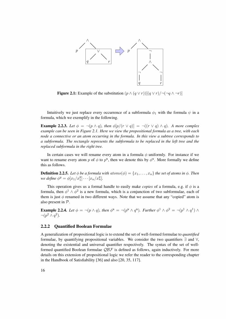
Figure 2.1: Example of the substitution (p ∧ (q ∨ r))[(q ∨ r)/¬(¬q ∧ ¬r)]

Intuitively we just replace every occurrence of a subformula φ1 with the formula ψ in aformula, which we exemplify in the following.

Example 2.2.3. Let φ = ¬(p ∧ q), then φ[p/(r ∨ q)] = ¬((r ∨ q) ∧ q). A more complexexample can be seen in Figure 2.1. Here we view the propositional formula as a tree, with eachnode a connective or an atom occurring in the formula. In this view a subtree corresponds toa subformula. The rectangle represents the subformula to be replaced in the left tree and thereplaced subformula in the right tree.

In certain cases we will rename every atom in a formula φ uniformly. For instance if wewant to rename every atom p of φ to pu, then we denote this by φu. More formally we definethis as follows.

Definition 2.2.5. Let φ be a formula with atoms(φ) = {x1, . . . , xn} the set of atoms in φ. Thenwe define φy = φ[x1/x

y1] · · · [xn/xyn].

This operation gives us a formal handle to easily make copies of a formula, e.g. if φ is aformula, then φ1 ∧ φ2 is a new formula, which is a conjunction of two subformulae, each ofthem is just φ renamed in two different ways. Note that we assume that any “copied” atom isalso present in P .

Example 2.2.4. Let φ = ¬(p ∧ q), then φu = ¬(pu ∧ qu). Further φ1 ∧ φ2 = ¬(p1 ∧ q1) ∧¬(p2 ∧ q2).

2.2.2 Quantified Boolean Formulae

A generalization of propositional logic is to extend the set of well-formed formulae to quantifiedformulae, by quantifying propositional variables. We consider the two quantifiers ∃ and ∀,denoting the existential and universal quantifier respectively. The syntax of the set of well-formed quantified Boolean formulae QBF is defined as follows, again inductively. For moredetails on this extension of propositional logic we refer the reader to the corresponding chapterin the Handbook of Satisfiability [36] and also [20, 35, 117].

16

Definition 2.2.6. Let P be a set of propositional atoms and WFFP the set of well-formedformulae built from P . We define QBFP inductively as follows.

• WFFP ⊆ QBFP ;

• if φ ∈ QBFP , then ¬φ ∈ QBFP ;

• if φ, ψ ∈ QBFP , then φ ◦ ψ ∈ QBFP for ◦ ∈ {∧,∨,→,←,↔}; and

• if φ ∈ QBFP and p ∈ P , then Qpφ ∈ QBFP for Q ∈ {∃,∀}.

As in the case ofWFF we usually omit the subscript for P if this is clear from the context.Further the order of the connectives for omitting parentheses is extended to include the newquantifiers. We order these two before the negation.

Example 2.2.5. The following formulae are in QBF: ∃p∀q(p ∨ q) and p ∧ ∃q ↔ p.

Unless noted otherwise we assume that a formula φ is inWFF and specifically mention ifa formula contains quantifiers, i.e. is in QBF \ WFF , if it is not clear from the context. Thevariable x of a quantifierQx is the quantified variable. For a sequence of the same quantifiers andtheir quantified variablesQx1 · · ·Qxnφ we use the shorthandQ{x1, . . . , xn}φ. In the followingwe assume that any quantified Boolean formula φ is well-formed, i.e. if φ is a formula withquantifiers, then φ ∈ QBF .

Another important concept is the scope of a quantified atom. A variable occurrence in aQBF may be either bound or free. Intuitively speaking a variable occurrence x is bound in φ ifit is in the scope of a quantifier, e.g. φ = Qxψ.

Definition 2.2.7. We define the function free : QBF → 2P recursively as follows, with φ, ψ,χ ∈ QBF:

• if φ ∈ P , then free(φ) = {φ};

• if φ ∈ {>,⊥}, then free(φ) = ∅;

• if φ = ¬ψ, then free(φ) = free(ψ);

• if φ = ψ ◦ χ, then free(ψ ◦ χ) = free(ψ) ∪ free(χ) if ◦ ∈ {∧, ∨,→,←,↔}; and

• if φ = Qxψ, then free(φ) = free(ψ) \ {x} for Q ∈ {∃,∀}.

A QBF φ is said to be open if free(φ) 6= ∅ and closed otherwise. Note that in the specialcase that a formula φ ∈ WFF does not contain quantifiers and no atoms of P , i.e. it containsonly connectives and symbols of {>, ⊥}, then this QBF is also closed.

Example 2.2.6. Let φ = ∃p(p ∧ q), ψ = ∃p¬p and χ = > ∨ ⊥, then all three φ, ψ and χare in QBF and the first one is open, while the other two are closed, i.e. free(φ) = {q} andfree(ψ) = ∅ = free(χ).

17

We define a slightly different renaming function for QBFs which acts only on free occur-rences of variables, which will be used for defining the semantics of QBFs.

Definition 2.2.8. We define the renaming function of free atoms in QBFs in postfix notation·[p/ψ]free , mapping QBFs to QBFs, recursively as follows, with φ, ψ, χ ∈ QBF and p ∈ P .

• p[p/ψ]free = ψ;

• x[p/ψ]free = x if p 6= x and x ∈ P ∪ {>,⊥};

• (¬φ)[p/ψ]free = ¬(φ[p/ψ]free);

• (φ ◦ χ)[p/ψ]free = (φ[p/ψ]free) ◦ (χ[p/ψ]free) for ◦ ∈ {∧,∨,→,←,↔};

• Qpφ[p/ψ]free = Qpφ for Q ∈ {∃, ∀}; and

• Qxφ[p/ψ]free = Qx(φ[p/ψ]free) if x 6= p for Q ∈ {∃, ∀}.

2.2.3 Normal Forms

Normal forms of logical formulae play a major role in both theory and practical solving. Thereason for this is a uniform structure of a formula in a certain normal form, which one can exploitto solve reasoning tasks on the formula. Moreover algorithms can be streamlined to work withsuch normal forms and allow for more efficiency. Many normal forms exist on logical formulae.We define the conjunctive normal form (CNF) for propositional formulae in WFF and theprenex normal form (PNF) of formulae in QBF . As we will see later in Section 2.2.4 anyformula inWFF can be rewritten to a CNF formula and any formula in QBF can be rewrittento a PNF formula while preserving important properties.

The basic building block for a formula in CNF is the literal. A literal is simply an elementof P ∪ {>,⊥} or its negation, i.e. ¬p for p ∈ P ∪ {>,⊥}. A disjunction of literals is called aclause. A CNF is now a conjunction of clauses.

Definition 2.2.9. Let φ be a formula. Then φ is

• a literal if φ = p or φ = ¬p for p ∈ P ∪ {>,⊥};

• a clause if φ = l1 ∨ · · · ∨ ln with l1, . . . , ln literals and n ≥ 0; or

• in conjunctive normal form (CNF) if φ = c1∧· · ·∧cm with c1, . . . , cm clauses andm ≥ 0.

Note that a formula may be literal, clause and in CNF at the same time. In particular a literalis always also a clause and a clause is always in CNF. Further we identify clauses with sets ofliterals and a formula in CNF by a set of clauses. An empty set of literals represents ⊥ and anempty set of clauses >. Consider the following example.

Example 2.2.7. Let φ = p, ψ = p ∨ ¬q ∨ r and χ = (p ∨ q) ∧ (¬p ∨ r). Then φ is aliteral, φ and ψ are clauses and all three φ, ψ and χ are in CNF. Alternatively we may write e.g.ψ = {{p,¬q, r}}. As an example for a formula not in CNF consider χ = (p ∧ r) → (q ∧ r).The formula χ is neither a literal, a clause nor in CNF.

18

For a formula with quantifiers a widely used normal form is the so-called prenex normalform. Intuitively a QBF is in PNF if the quantifiers are all collected left of the formula.

Definition 2.2.10. Let φ be a QBF, ψ ∈ WFF , Qi ∈ {∃,∀} for 1 ≤ i ≤ n and {x1, . . . xn} ⊆P . Then φ is in prenex normal form (PNF) if φ = Q1x1 · · ·Qnxnψ.

Classes of PNFs which are of special interest in our work are QBFs in PNF which beginwith a certain quantifier and then have n quantifier “alternations”, meaning that we start withe.g. ∃, followed possibly by several ∃ quantifiers, then have one or more ∀ quantifiers and thenone or more ∃ quantifiers and so on until we have n alternations between quantifiers. If we haveonly one quantifier then n = 1. As we will see later in Section 2.4, these classes can be used forcharacterization of certain complexity classes.

Definition 2.2.11. Let φ be a QBF in PNF, ψ ∈ WFF , n > 0 an integer and Xi ⊆ P for1 ≤ i ≤ n. The formula φ is

• in QBF∃,n if φ = ∃X1∀X2∃X3 · · ·QXnψ with Q = ∃ if n is odd and Q = ∀ else, or

• in QBF∀,n if φ = ∀X1∃X2∀X3 · · ·QXnψ with Q = ∀ if n is odd and Q = ∃ else.

Example 2.2.8. Let ψ ∈ WFF and φ = ∃{x1, x2}∀{x3, x4, x5}∃{x6}ψ. Then φ ∈ QBF∃,3and φ is in PNF.

2.2.4 Semantics

In this section we introduce the logical semantics of propositional logic with quantifiers. Firstwe deal with the classical approach. Here the very basic idea is that every proposition can betrue or false. This means we can assign to each proposition a truth value. In classical logic wehave two truth values: true, which we denote with the constant ’t’ and false, which we denote as’f ’. Further we introduce the semantics of three-valued propositional logic which includes thetruth value undecided or unknown, which we write as ’u’. Three-valued semantics for QBFs canalso be defined, but we do not require such a semantics for our work. Hence we only introducethe three-valued semantics for unquantified propositional logic.

The most important concept for the semantics we use here is called the interpretation func-tion.

Definition 2.2.12. Let V ⊆ {t, f ,u}. An interpretation I is a function I : P → V . If V = {t, f}then I is two-valued. If V = {t, f ,u} then I is three-valued.

We only consider two or three-valued interpretations. We usually say that an interpretationis defined directly on a set of atoms or on a formula or omit this information if it is clear fromthe context, i.e. if I is defined on a propositional formula φ, then we mean I is defined onatoms(φ). For a QBF φ we define interpretations on free(φ). Note that in case I is defined onφ ∈ QBF , then dom(I) = ∅ if φ is closed. We use the symbols I, J,K, . . . for interpretationsand I,J ,K for sets of interpretations. In the following, unless noted otherwise, we assumethat an interpretation I is two-valued. By a partial interpretation I on a set S we mean thatdom(I) ⊆ S.

19

Interpretations can equivalently be represented as sets or as a triple of sets, depending if theyare two or three-valued. First we define this handy shortcut for the set of atoms mapped to acertain truth value.

Definition 2.2.13. Let I be an interpretation defined on the set X and v ∈ {t, f ,u}. We defineIv = {x | I(x) = v}.

Now we can view a two-valued interpretation I also as the set It. This set defines theassignment as follows, if I is defined on X , then every element in the set It is assigned true byI and every element in X \ It = If is assigned false (or in case of unrestricted domain P \ It).A three-valued interpretation I can be presented equivalently by the triple (It, If , Iu).

An interpretation I on a formula φ represents a particular logical view on the propositions inthe formula, meaning that certain propositions are assigned true, false or undecided. A formulacan be evaluated under an interpretation defined on it. Such a formula evaluates to a unique truthvalue under the interpretation. This unique value represents the truth value of the formula giventhe logical view on the propositional atoms defined via the interpretation function. We beginwith the two-valued scenario. By a slight abuse of notation, which will be convenient, we applyI not only on atoms, but also on formulae, i.e. I(φ) denotes the evaluation of φ under I .

Definition 2.2.14. Let φ ∈ QBF , ψ and χ be subformulae of φ, x ∈ P and I a two-valuedinterpretation on φ. The evaluation of φ under I , denoted as I(φ) is defined recursively asfollows.

• if φ = p, p ∈ P , then I(φ) = I(p),

• if φ = >, then I(φ) = t,

• if φ = ⊥, then I(φ) = f ,

• if φ = ¬ψ, then I(φ) = t iff I(ψ) = f ,

• if φ = ψ ∧ χ, then I(φ) = t iff I(ψ) = I(χ) = t,

• if φ = ψ ∨ χ, then I(φ) = t iff I(ψ) = t or I(χ) = t,

• if φ = ψ → χ, then I(φ) = t iff I(ψ) = f or I(χ) = t,

• if φ = ψ ← χ, then I(φ) = t iff I(ψ) = t or I(χ) = f ,

• if φ = ψ ↔ χ, then I(φ) = t iff I(ψ) = I(χ),

• if φ = ∃xψ, then I(φ) = t iff I(ψ[x/>]free) = t or I(ψ[x/⊥]free) = t,

• if φ = ∀xψ, then I(φ) = t iff I(ψ[x/>]free) = t and I(ψ[x/⊥]free) = t.

If I(φ) 6= t, then I(φ) = f .

20

¬t ff t

∨ t f

t t tf t f

∧ t f

t t ff f f

→ t f

t t ff t t

↔ t f

t t ff f t

Figure 2.2: Truth tables for classical two–valued logic

a b c ¬c (b ∨ ¬c) a ∧ (b ∨ ¬c)f f f t t ff f t f f ff t f t t ff t t f t ft f f t t tt f t f f ft t f t t tt t t f t t

Figure 2.3: Truth table for the formula a ∧ (b ∨ ¬c)

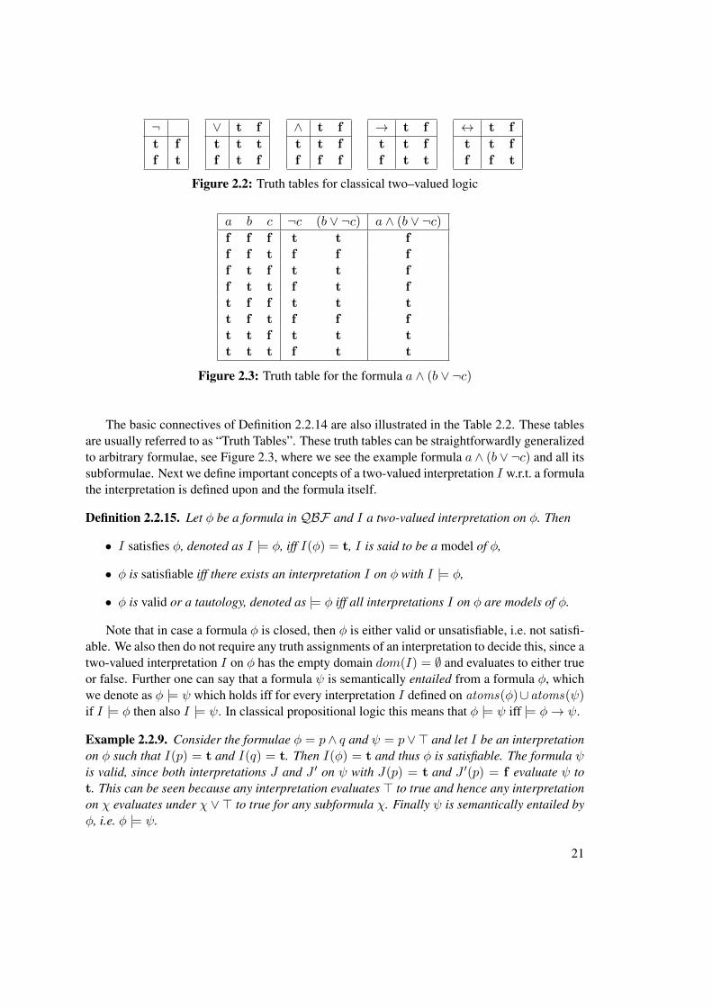
The basic connectives of Definition 2.2.14 are also illustrated in the Table 2.2. These tablesare usually referred to as “Truth Tables”. These truth tables can be straightforwardly generalizedto arbitrary formulae, see Figure 2.3, where we see the example formula a ∧ (b ∨ ¬c) and all itssubformulae. Next we define important concepts of a two-valued interpretation I w.r.t. a formulathe interpretation is defined upon and the formula itself.

Definition 2.2.15. Let φ be a formula in QBF and I a two-valued interpretation on φ. Then

• I satisfies φ, denoted as I |= φ, iff I(φ) = t, I is said to be a model of φ,

• φ is satisfiable iff there exists an interpretation I on φ with I |= φ,

• φ is valid or a tautology, denoted as |= φ iff all interpretations I on φ are models of φ.

Note that in case a formula φ is closed, then φ is either valid or unsatisfiable, i.e. not satisfi-able. We also then do not require any truth assignments of an interpretation to decide this, since atwo-valued interpretation I on φ has the empty domain dom(I) = ∅ and evaluates to either trueor false. Further one can say that a formula ψ is semantically entailed from a formula φ, whichwe denote as φ |= ψ which holds iff for every interpretation I defined on atoms(φ)∪atoms(ψ)if I |= φ then also I |= ψ. In classical propositional logic this means that φ |= ψ iff |= φ→ ψ.

Example 2.2.9. Consider the formulae φ = p∧ q and ψ = p∨> and let I be an interpretationon φ such that I(p) = t and I(q) = t. Then I(φ) = t and thus φ is satisfiable. The formula ψis valid, since both interpretations J and J ′ on ψ with J(p) = t and J ′(p) = f evaluate ψ tot. This can be seen because any interpretation evaluates > to true and hence any interpretationon χ evaluates under χ ∨ > to true for any subformula χ. Finally ψ is semantically entailed byφ, i.e. φ |= ψ.

21

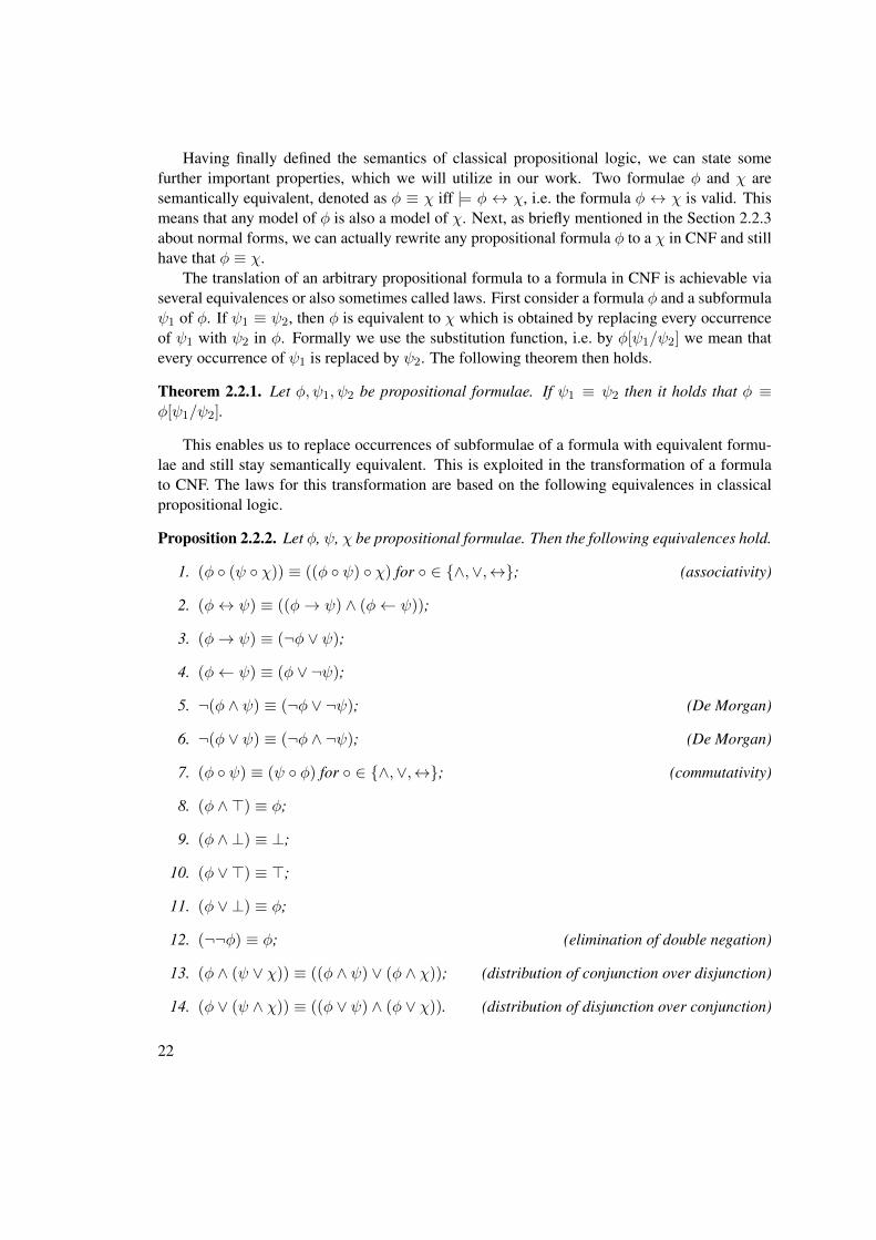
Having finally defined the semantics of classical propositional logic, we can state somefurther important properties, which we will utilize in our work. Two formulae φ and χ aresemantically equivalent, denoted as φ ≡ χ iff |= φ ↔ χ, i.e. the formula φ ↔ χ is valid. Thismeans that any model of φ is also a model of χ. Next, as briefly mentioned in the Section 2.2.3about normal forms, we can actually rewrite any propositional formula φ to a χ in CNF and stillhave that φ ≡ χ.

The translation of an arbitrary propositional formula to a formula in CNF is achievable viaseveral equivalences or also sometimes called laws. First consider a formula φ and a subformulaψ1 of φ. If ψ1 ≡ ψ2, then φ is equivalent to χ which is obtained by replacing every occurrenceof ψ1 with ψ2 in φ. Formally we use the substitution function, i.e. by φ[ψ1/ψ2] we mean thatevery occurrence of ψ1 is replaced by ψ2. The following theorem then holds.

Theorem 2.2.1. Let φ, ψ1, ψ2 be propositional formulae. If ψ1 ≡ ψ2 then it holds that φ ≡φ[ψ1/ψ2].

This enables us to replace occurrences of subformulae of a formula with equivalent formu-lae and still stay semantically equivalent. This is exploited in the transformation of a formulato CNF. The laws for this transformation are based on the following equivalences in classicalpropositional logic.

Proposition 2.2.2. Let φ, ψ, χ be propositional formulae. Then the following equivalences hold.

1. (φ ◦ (ψ ◦ χ)) ≡ ((φ ◦ ψ) ◦ χ) for ◦ ∈ {∧,∨,↔}; (associativity)

2. (φ↔ ψ) ≡ ((φ→ ψ) ∧ (φ← ψ));

3. (φ→ ψ) ≡ (¬φ ∨ ψ);

4. (φ← ψ) ≡ (φ ∨ ¬ψ);

5. ¬(φ ∧ ψ) ≡ (¬φ ∨ ¬ψ); (De Morgan)

6. ¬(φ ∨ ψ) ≡ (¬φ ∧ ¬ψ); (De Morgan)

7. (φ ◦ ψ) ≡ (ψ ◦ φ) for ◦ ∈ {∧,∨,↔}; (commutativity)

8. (φ ∧ >) ≡ φ;

9. (φ ∧ ⊥) ≡ ⊥;

10. (φ ∨ >) ≡ >;

11. (φ ∨ ⊥) ≡ φ;

12. (¬¬φ) ≡ φ; (elimination of double negation)

13. (φ ∧ (ψ ∨ χ)) ≡ ((φ ∧ ψ) ∨ (φ ∧ χ)); (distribution of conjunction over disjunction)

14. (φ ∨ (ψ ∧ χ)) ≡ ((φ ∨ ψ) ∧ (φ ∨ χ)). (distribution of disjunction over conjunction)

22

We can use these equivalences for successively rewriting a formula to a formula in CNF.Essentially these equivalences can be read as “rewriting rules”, e.g. if we encounter a subformulaof the form shown on the left, we rewrite all these subformulae to a form shown on the right.If we apply these exhaustively, except for the associativity and commutativity rules, then theresulting formula is in CNF. This rewriting in general may lead to a drastically larger formulain CNF. For this purpose Tseitin [149] proposed another transformation, which transforms aformula φ to χ, such that φ is satisfiable iff χ is satisfiable, but we in general do not have thatφ ≡ χ. The benefit of this translation is that the size of χ, i.e. the number of symbols in theformula, does not increase exponentially w.r.t. the size of φ in the worst case, as is the case withstandard translation, but is only polynomial with the Tseitin translation. Regarding QBFs wecan rewrite every QBF φ to a QBF χ such that χ is in PNF and φ ≡ χ.

Example 2.2.10. Let φ = ¬(a∨ b)∨¬c. Then we can transform φ to χ1 = (¬a∧¬b)∨¬c andin a second step to χ2 = (¬a ∨ ¬c) ∧ (¬b ∨ ¬c), which is in CNF and φ ≡ χ1 ≡ χ2.

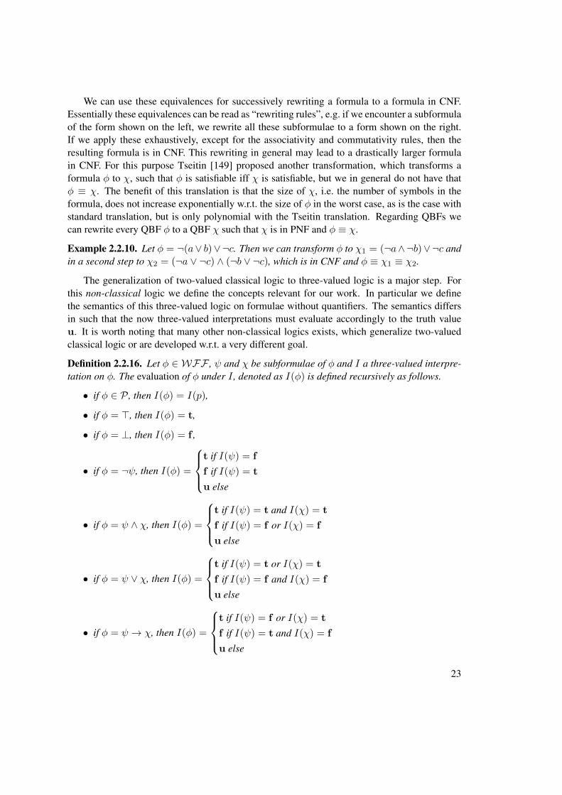
The generalization of two-valued classical logic to three-valued logic is a major step. Forthis non-classical logic we define the concepts relevant for our work. In particular we definethe semantics of this three-valued logic on formulae without quantifiers. The semantics differsin such that the now three-valued interpretations must evaluate accordingly to the truth valueu. It is worth noting that many other non-classical logics exists, which generalize two-valuedclassical logic or are developed w.r.t. a very different goal.

Definition 2.2.16. Let φ ∈ WFF , ψ and χ be subformulae of φ and I a three-valued interpre-tation on φ. The evaluation of φ under I , denoted as I(φ) is defined recursively as follows.

• if φ ∈ P , then I(φ) = I(p),

• if φ = >, then I(φ) = t,

• if φ = ⊥, then I(φ) = f ,

• if φ = ¬ψ, then I(φ) =

t if I(ψ) = f

f if I(ψ) = t

u else

• if φ = ψ ∧ χ, then I(φ) =

t if I(ψ) = t and I(χ) = t

f if I(ψ) = f or I(χ) = f

u else

• if φ = ψ ∨ χ, then I(φ) =

t if I(ψ) = t or I(χ) = t

f if I(ψ) = f and I(χ) = f

u else

• if φ = ψ → χ, then I(φ) =

t if I(ψ) = f or I(χ) = t

f if I(ψ) = t and I(χ) = f

u else

23

¬t ff tu u

∨ t u f

t t t tu t u uf t u f

∧ t u f

t t u fu u u ff f f f

→ t u f

t t u fu t u uf t t t

↔ t u f

t t u fu u u uf f u t

Figure 2.4: Truth tables for strong three–valued logic of Kleene

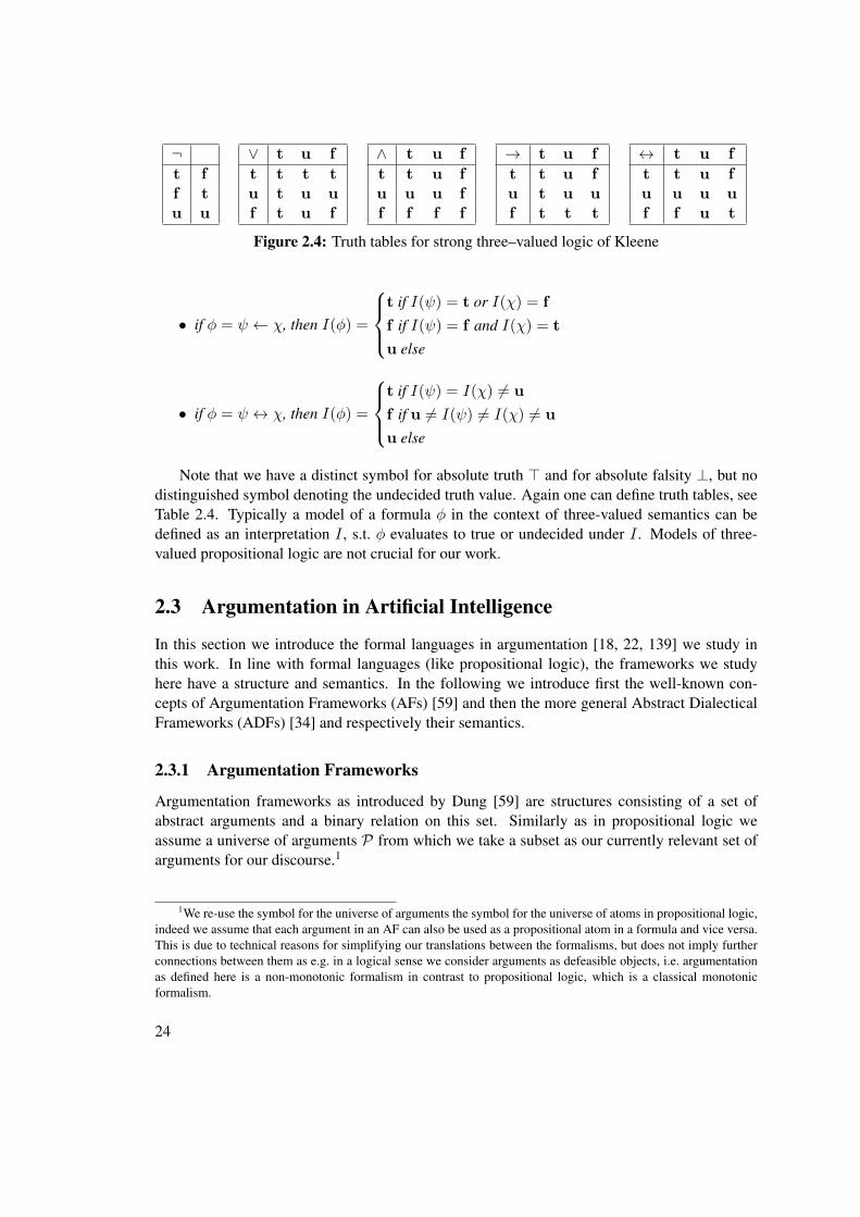
• if φ = ψ ← χ, then I(φ) =

t if I(ψ) = t or I(χ) = f

f if I(ψ) = f and I(χ) = t

u else

• if φ = ψ ↔ χ, then I(φ) =

t if I(ψ) = I(χ) 6= u

f if u 6= I(ψ) 6= I(χ) 6= u

u else

Note that we have a distinct symbol for absolute truth > and for absolute falsity ⊥, but nodistinguished symbol denoting the undecided truth value. Again one can define truth tables, seeTable 2.4. Typically a model of a formula φ in the context of three-valued semantics can bedefined as an interpretation I , s.t. φ evaluates to true or undecided under I . Models of three-valued propositional logic are not crucial for our work.

2.3 Argumentation in Artificial Intelligence

In this section we introduce the formal languages in argumentation [18, 22, 139] we study inthis work. In line with formal languages (like propositional logic), the frameworks we studyhere have a structure and semantics. In the following we introduce first the well-known con-cepts of Argumentation Frameworks (AFs) [59] and then the more general Abstract DialecticalFrameworks (ADFs) [34] and respectively their semantics.

2.3.1 Argumentation Frameworks

Argumentation frameworks as introduced by Dung [59] are structures consisting of a set ofabstract arguments and a binary relation on this set. Similarly as in propositional logic weassume a universe of arguments P from which we take a subset as our currently relevant set ofarguments for our discourse.1

1We re-use the symbol for the universe of arguments the symbol for the universe of atoms in propositional logic,indeed we assume that each argument in an AF can also be used as a propositional atom in a formula and vice versa.This is due to technical reasons for simplifying our translations between the formalisms, but does not imply furtherconnections between them as e.g. in a logical sense we consider arguments as defeasible objects, i.e. argumentationas defined here is a non-monotonic formalism in contrast to propositional logic, which is a classical monotonicformalism.

24

a

b

c d

e

Figure 2.5: Example argumentation framework F

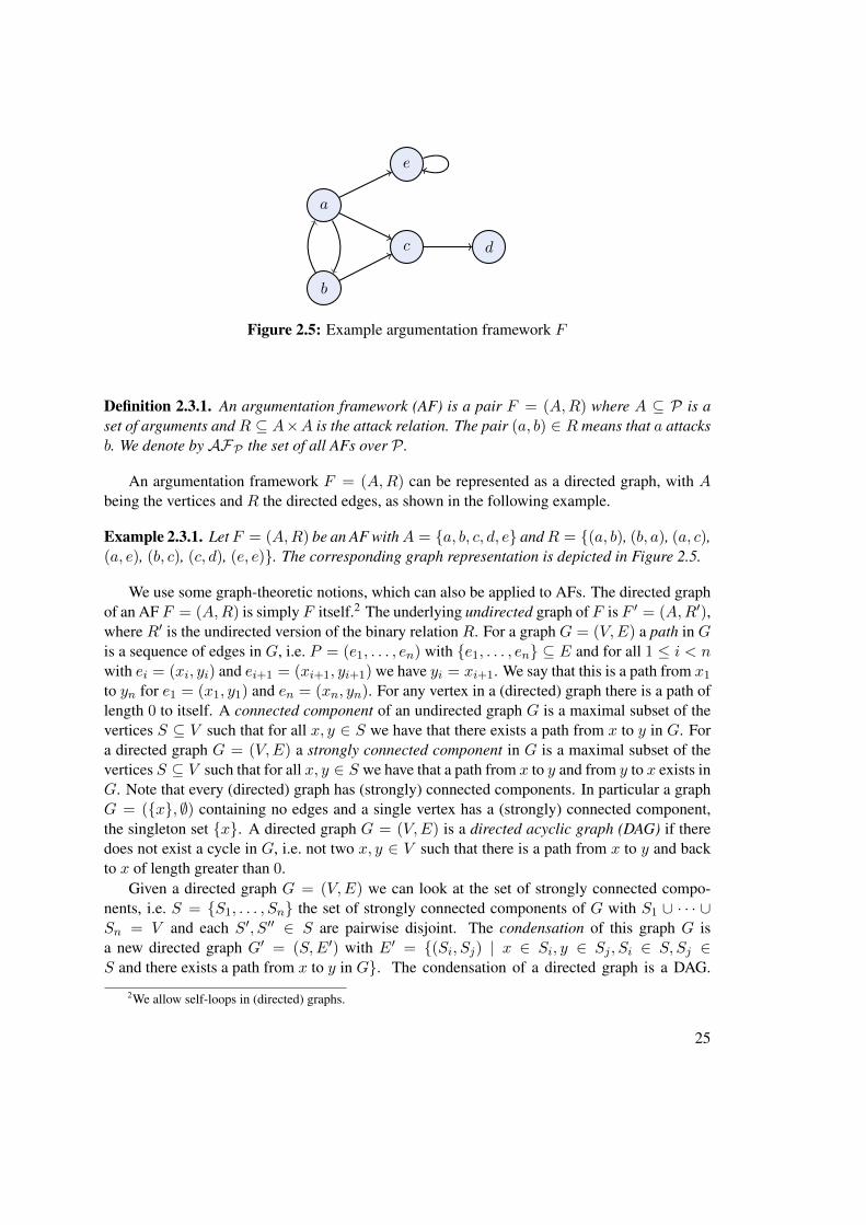
Definition 2.3.1. An argumentation framework (AF) is a pair F = (A,R) where A ⊆ P is aset of arguments and R ⊆ A×A is the attack relation. The pair (a, b) ∈ R means that a attacksb. We denote by AFP the set of all AFs over P .

An argumentation framework F = (A,R) can be represented as a directed graph, with Abeing the vertices and R the directed edges, as shown in the following example.

Example 2.3.1. Let F = (A,R) be an AF withA = {a, b, c, d, e} andR = {(a, b), (b, a), (a, c),(a, e), (b, c), (c, d), (e, e)}. The corresponding graph representation is depicted in Figure 2.5.

We use some graph-theoretic notions, which can also be applied to AFs. The directed graphof an AF F = (A,R) is simply F itself.2 The underlying undirected graph of F is F ′ = (A,R′),where R′ is the undirected version of the binary relation R. For a graph G = (V,E) a path in Gis a sequence of edges in G, i.e. P = (e1, . . . , en) with {e1, . . . , en} ⊆ E and for all 1 ≤ i < nwith ei = (xi, yi) and ei+1 = (xi+1, yi+1) we have yi = xi+1. We say that this is a path from x1

to yn for e1 = (x1, y1) and en = (xn, yn). For any vertex in a (directed) graph there is a path oflength 0 to itself. A connected component of an undirected graph G is a maximal subset of thevertices S ⊆ V such that for all x, y ∈ S we have that there exists a path from x to y in G. Fora directed graph G = (V,E) a strongly connected component in G is a maximal subset of thevertices S ⊆ V such that for all x, y ∈ S we have that a path from x to y and from y to x exists inG. Note that every (directed) graph has (strongly) connected components. In particular a graphG = ({x}, ∅) containing no edges and a single vertex has a (strongly) connected component,the singleton set {x}. A directed graph G = (V,E) is a directed acyclic graph (DAG) if theredoes not exist a cycle in G, i.e. not two x, y ∈ V such that there is a path from x to y and backto x of length greater than 0.

Given a directed graph G = (V,E) we can look at the set of strongly connected compo-nents, i.e. S = {S1, . . . , Sn} the set of strongly connected components of G with S1 ∪ · · · ∪Sn = V and each S′, S′′ ∈ S are pairwise disjoint. The condensation of this graph G isa new directed graph G′ = (S,E′) with E′ = {(Si, Sj) | x ∈ Si, y ∈ Sj , Si ∈ S, Sj ∈S and there exists a path from x to y in G}. The condensation of a directed graph is a DAG.

2We allow self-loops in (directed) graphs.

25

{a, b}

{c} {d}

{e}

Figure 2.6: Condensation of AF from Example 2.3.1

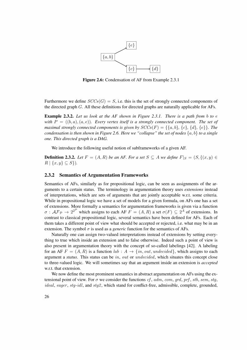
Furthermore we define SCCs(G) = S, i.e. this is the set of strongly connected components ofthe directed graph G. All these definitions for directed graphs are naturally applicable for AFs.

Example 2.3.2. Let us look at the AF shown in Figure 2.3.1. There is a path from b to ewith P = ((b, a), (a, e)). Every vertex itself is a strongly connected component. The set ofmaximal strongly connected components is given by SCCs(F ) = {{a, b}, {c}, {d}, {e}}. Thecondensation is then shown in Figure 2.6. Here we “collapse” the set of nodes {a, b} to a singleone. This directed graph is a DAG.

We introduce the following useful notion of subframeworks of a given AF.

Definition 2.3.2. Let F = (A,R) be an AF. For a set S ⊆ A we define F |S = (S, {(x, y) ∈R | {x, y} ⊆ S}).

2.3.2 Semantics of Argumentation Frameworks

Semantics of AFs, similarly as for propositional logic, can be seen as assignments of the ar-guments to a certain status. The terminology in argumentation theory uses extensions insteadof interpretations, which are sets of arguments that are jointly acceptable w.r.t. some criteria.While in propositional logic we have a set of models for a given formula, on AFs one has a setof extensions. More formally a semantics for argumentation frameworks is given via a functionσ : AFP → 22P which assigns to each AF F = (A,R) a set σ(F ) ⊆ 2A of extensions. Incontrast to classical propositional logic, several semantics have been defined for AFs. Each ofthem takes a different point of view what should be accepted or rejected, i.e. what may be in anextension. The symbol σ is used as a generic function for the semantics of AFs.

Naturally one can assign two-valued interpretations instead of extensions by setting every-thing to true which inside an extension and to false otherwise. Indeed such a point of view isalso present in argumentation theory with the concept of so-called labelings [42]. A labelingfor an AF F = (A,R) is a function lab : A → {in, out , undecided}, which assigns to eachargument a status. This status can be in , out or undecided , which situates this concept closeto three-valued logic. We will sometimes say that an argument inside an extension is acceptedw.r.t. that extension.

We now define the most prominent semantics in abstract argumentation on AFs using the ex-tensional point of view. For σ we consider the functions cf , adm , com , grd , prf , stb, sem , stg ,ideal , eager , stg-idl , and stg2 , which stand for conflict-free, admissible, complete, grounded,

26

preferred, stable, semi-stable, stage, ideal, eager, stage-ideal, and stage2 extensions, respec-tively. Conflict-free, admissible, complete, grounded, preferred and stable semantics have beenintroduced in [59], semi-stable semantics in [37, 41], stage in [151], ideal in [60], eager in [39],stage-ideal in [67] and stage2 in [72]. The semantics for the three-valued labelings can be definedaccordingly and we exemplarily show the corresponding definition for the complete semantics.

The basic concept for many of the semantics considered in this work is the admissible ex-tension or just admissible set. Admissibility has two requirements, namely conflict-freeness anddefense of all arguments in the set.

Definition 2.3.3. Let F = (A,R) be an AF. A set S ⊆ A is conflict-free in F , if there are noa, b ∈ S, such that (a, b) ∈ R. We say that an argument a ∈ A is defended by a set S ⊆ A in Fif, for each b ∈ A such that (b, a) ∈ R, there exists a c ∈ S such that (c, b) ∈ R.

Formally an argument a is defended by a set of arguments if all attackers of a are counter-attacked by arguments in the set. If for instance we accept the set of arguments then, intuitivelyspeaking, we disagree or reject all attackers of a, since they are attacked. In turn it is reasonablein this framework to view the argument a as acceptable, too. Admissible sets are then conflict-free sets of arguments, where each argument in the set is defended by the set.

Definition 2.3.4. Let F = (A,R) be an AF. A set S ⊆ A is admissible in F , if

• S is conflict-free in F ; and

• each a ∈ S is defended by S in F .

Complete extensions are admissible sets which contain every argument they defend, i.e. theyare complete in the sense that every defended argument is also accepted, that is, in the set.

Definition 2.3.5. Let F = (A,R) be an AF. An admissible set S ⊆ A in F is a completeextension in F , if every s ∈ A which is defended by S in F is in S.

There is a useful equivalent definition of defense and the concepts of admissibility and com-plete extensions. It is based on the characteristic function of an AF. Given a set of arguments,this function returns every argument defended by this set.

Definition 2.3.6. Let F = (A,R) be an AF and S ⊆ A. Then FF : 2A → 2A is the character-istic function of F and is defined by FF (S) = {a | a is defended by S}.

If we consider for an AF F = (A,R) the partially ordered set (2A,⊆), then FF is ⊆-monotone.

Lemma 2.3.1 ([59, Lemma 19]). Let F = (A,R) be an AF. FF is ⊆-monotone.

Using this function we can define the admissible sets and complete extensions as follows.

Proposition 2.3.2 ([59, Lemma 18 and Lemma 24]). Let F = (A,R) be an AF. For a conflict-free set S ∈ cf (F ), it holds that

• S ∈ adm(F ) iff S ⊆ FF (S);

27

• S ∈ com(F ) iff S = FF (S).

The minimal complete extension, w.r.t. subset-inclusion is referred to as the grounded ex-tension.

Definition 2.3.7. Let F = (A,R) be an AF. A complete extension S ⊆ A in F is the groundedextension in F , if there is no complete extension S′ ⊆ A in F such that S′ ( S.

The grounded extension is also the least fixed point of the characteristic function and thus isunique.

Proposition 2.3.3. Let F = (A,R) be an AF. The grounded extension S ∈ grd(F ) is the leastfixed point of FF .

Maximal admissible sets, w.r.t. subset-inclusion are called preferred extensions and acceptas many arguments as possible, without violating admissibility.

Definition 2.3.8. Let F = (A,R) be an AF. An admissible set S ⊆ A in F is a preferredextension in F , if there is no admissible set S′ ⊆ A in F such that S ( S′.

Note that we could equivalently define the preferred extension to be maximal complete ex-tensions w.r.t. subset-inclusion. A basic property of the preferred semantics is that admissiblesets, complete extensions and hence preferred extensions and the grounded extension always ex-ist for any given framework. This follows in particular due to the fact that the empty set is alwaysadmissible in any AF. A popular semantics for which this is not the case is the stable semantics.For the definition of the stable semantics and the closely related semi-stable and stage semanticswe make use of the concept of the range of a given set S of arguments, which is simply the setitself and everything it attacks,

Definition 2.3.9. Let F = (A,R) be an AF and S ⊆ A. The range of S (in R), denoted by S+R ,

is given by S+R = S ∪ {a | (b, a) ∈ R, b ∈ S}.

Then a set is stable if it is conflict-free and attacks everything not contained in it, i.e. itsrange covers all arguments in the framework. Semi-stable extensions are admissible sets whichhave a subset maximal range, while stage extensions are conflict-free sets with subset maximalrange.

Definition 2.3.10. Let F = (A,R) be an AF. A conflict-free set S ⊆ A in F is a stable extensionin F , if S+

R = A. An admissible set E in F is a semi-stable extension in F if there does not exista set T admissible in F , with E+

R ⊂ T+R . A conflict-free set E in F is a stage extension in F if

there does not exist a set T conflict-free in F , with E+R ⊂ T+

R .

A basic property of semi-stable and stage semantics is that if an AF has stable extensions,then the semi-stable, stage and stable semantics coincide [41]. The intuition is that semi-stableand stage extensions should be “close” to stable extensions, in case no stable extensions exist.

Regarding the aforementioned labeling approach, we can use a three-valued interpretationfor defining complete semantics in the following manner [42].3

3Our definition diverges from the original in [42] by identifying in = t, out = f and undec = u.

28

Definition 2.3.11. Let F = (A,R) be an AF. A function I : A → {t, f ,u} is a completelabeling in F iff the following conditions hold for each a ∈ A.

• I(a) = t iff for each b with (b, a) ∈ R we have I(b) = f ; and

• I(a) = f iff there exists a b with (b, a) ∈ R we have I(b) = t

Other semantics we defined here can likewise be defined using labelings. We further havethe following correspondence.

Proposition 2.3.4 ([42, Theorem 9 and Theorem 10]). Let F = (A,R) be an AF. It holds thatcom(F ) = {It | I a complete labeling in F}.

That is, we can immediately infer a complete labeling from a complete extension and viceversa. Given an AF F = (A,R) and E ∈ com(F ) and E+ = E+

R \ E, then the following isa complete labeling: (E,E+, A \ (E+

R )). The other direction is is even more simpler, given athree-valued complete labeling I of F , then It is a complete extension.

Example 2.3.3. Consider the AF F from Example 2.3.1. Then we have the following conflict-free sets, admissible sets and extensions of the semantics:

• cf (F ) = {∅, {a}, {b}, {c}, {d}, {a, d}, {b, d}};

• adm(F ) = {∅, {a}, {b}, {a, d},{b, d}};

• com(F ) = {∅, {a, d}, {b, d}};

• grd(F ) = {∅};

• stb(F ) = {{a, d}};

• prf (F ) = {{a, d}, {b, d}};

• sem(F ) = {{a, d}}; and

• stg(F ) = {{a, d}}.

The complete labelings of F are given by {(∅, ∅ ,{a, b, c, d, e}), ({a, d}, {b, c, e}, ∅), ({b, d},{a, b, e}, ∅)}. Here we see that the empty extension is the grounded extension of the frameworkand corresponds to {(∅, ∅ ,{a, b, c, d, e}), i.e. setting all arguments to undecided.

Note that if we would add a single isolated self-attacking argument to F , i.e. F ′ = (A′, R′)with A′ = A ∪ {f} and R′ = R ∪ {(f, f)}, shown in Figure 2.7, then stb(F ′) = ∅, but theset of semi-stable and stage extensions would remain the same, i.e. sem(F ′) = sem(F ) andstg(F ) = stg(F ′).

Although this may appear as a deficiency of stable semantics, we can see on the AF F aninteresting concept, namely that the preferred extension {b, d} is not stable, because it does notattack the self-attacking argument e. Such a self-attacking argument ensures that any stableextension necessarily must accept in the extension an attacker of it. This behavior can be usedfor modeling certain situations, e.g. if we require that in any stable extension one argument out

29

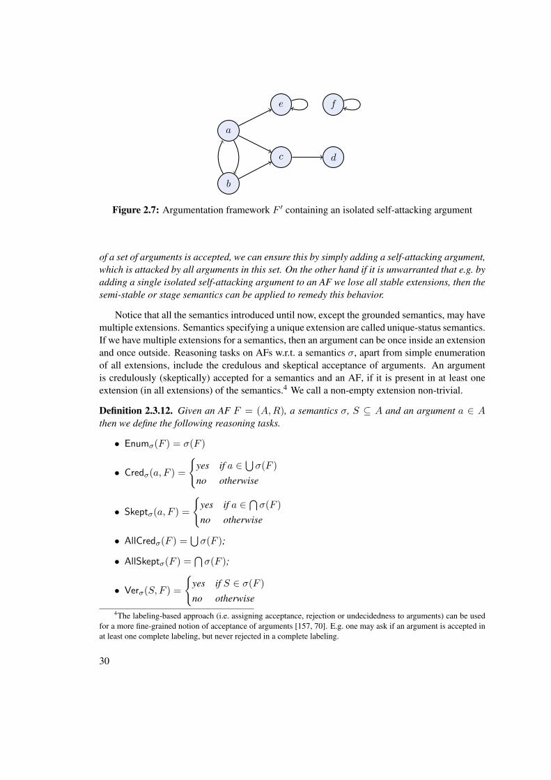
a

b

c d

e f

Figure 2.7: Argumentation framework F ′ containing an isolated self-attacking argument

of a set of arguments is accepted, we can ensure this by simply adding a self-attacking argument,which is attacked by all arguments in this set. On the other hand if it is unwarranted that e.g. byadding a single isolated self-attacking argument to an AF we lose all stable extensions, then thesemi-stable or stage semantics can be applied to remedy this behavior.

Notice that all the semantics introduced until now, except the grounded semantics, may havemultiple extensions. Semantics specifying a unique extension are called unique-status semantics.If we have multiple extensions for a semantics, then an argument can be once inside an extensionand once outside. Reasoning tasks on AFs w.r.t. a semantics σ, apart from simple enumerationof all extensions, include the credulous and skeptical acceptance of arguments. An argumentis credulously (skeptically) accepted for a semantics and an AF, if it is present in at least oneextension (in all extensions) of the semantics.4 We call a non-empty extension non-trivial.

Definition 2.3.12. Given an AF F = (A,R), a semantics σ, S ⊆ A and an argument a ∈ Athen we define the following reasoning tasks.

• Enumσ(F ) = σ(F )

• Credσ(a, F ) =

{yes if a ∈ ⋃σ(F )

no otherwise

• Skeptσ(a, F ) =

{yes if a ∈ ⋂σ(F )

no otherwise

• AllCredσ(F ) =⋃σ(F );

• AllSkeptσ(F ) =⋂σ(F );

• Verσ(S, F ) =

{yes if S ∈ σ(F )

no otherwise4The labeling-based approach (i.e. assigning acceptance, rejection or undecidedness to arguments) can be used

for a more fine-grained notion of acceptance of arguments [157, 70]. E.g. one may ask if an argument is accepted inat least one complete labeling, but never rejected in a complete labeling.

30

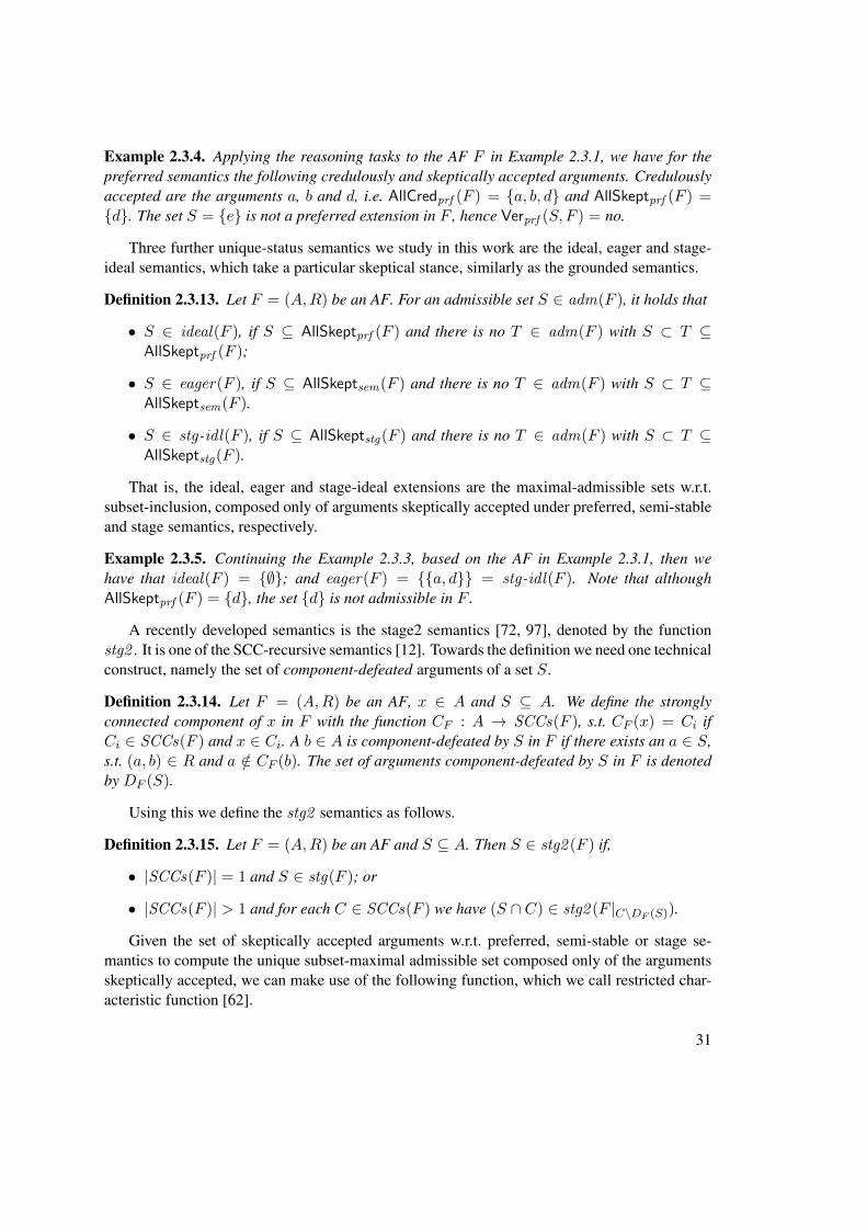
Example 2.3.4. Applying the reasoning tasks to the AF F in Example 2.3.1, we have for thepreferred semantics the following credulously and skeptically accepted arguments. Credulouslyaccepted are the arguments a, b and d, i.e. AllCredprf (F ) = {a, b, d} and AllSkeptprf (F ) ={d}. The set S = {e} is not a preferred extension in F , hence Verprf (S, F ) = no.

Three further unique-status semantics we study in this work are the ideal, eager and stage-ideal semantics, which take a particular skeptical stance, similarly as the grounded semantics.

Definition 2.3.13. Let F = (A,R) be an AF. For an admissible set S ∈ adm(F ), it holds that

• S ∈ ideal(F ), if S ⊆ AllSkeptprf (F ) and there is no T ∈ adm(F ) with S ⊂ T ⊆AllSkeptprf (F );

• S ∈ eager(F ), if S ⊆ AllSkeptsem(F ) and there is no T ∈ adm(F ) with S ⊂ T ⊆AllSkeptsem(F ).

• S ∈ stg-idl(F ), if S ⊆ AllSkeptstg(F ) and there is no T ∈ adm(F ) with S ⊂ T ⊆AllSkeptstg(F ).

That is, the ideal, eager and stage-ideal extensions are the maximal-admissible sets w.r.t.subset-inclusion, composed only of arguments skeptically accepted under preferred, semi-stableand stage semantics, respectively.

Example 2.3.5. Continuing the Example 2.3.3, based on the AF in Example 2.3.1, then wehave that ideal(F ) = {∅}; and eager(F ) = {{a, d}} = stg-idl(F ). Note that althoughAllSkeptprf (F ) = {d}, the set {d} is not admissible in F .

A recently developed semantics is the stage2 semantics [72, 97], denoted by the functionstg2 . It is one of the SCC-recursive semantics [12]. Towards the definition we need one technicalconstruct, namely the set of component-defeated arguments of a set S.

Definition 2.3.14. Let F = (A,R) be an AF, x ∈ A and S ⊆ A. We define the stronglyconnected component of x in F with the function CF : A → SCCs(F ), s.t. CF (x) = Ci ifCi ∈ SCCs(F ) and x ∈ Ci. A b ∈ A is component-defeated by S in F if there exists an a ∈ S,s.t. (a, b) ∈ R and a /∈ CF (b). The set of arguments component-defeated by S in F is denotedby DF (S).

Using this we define the stg2 semantics as follows.

Definition 2.3.15. Let F = (A,R) be an AF and S ⊆ A. Then S ∈ stg2 (F ) if,

• |SCCs(F )| = 1 and S ∈ stg(F ); or

• |SCCs(F )| > 1 and for each C ∈ SCCs(F ) we have (S ∩ C) ∈ stg2 (F |C\DF (S)).

Given the set of skeptically accepted arguments w.r.t. preferred, semi-stable or stage se-mantics to compute the unique subset-maximal admissible set composed only of the argumentsskeptically accepted, we can make use of the following function, which we call restricted char-acteristic function [62].

31

stable

stagestage2 semi-stable

preferred

complete

ideal

eager

admissible grounded

conflict-free

Figure 2.8: Relation between AF semantics

Definition 2.3.16. LetF = (A,R) be an AF. Then FF : 2A → 2A is the restricted characteristicfunction of F and is defined by FF (S) = {a ∈ S | a is defended by S}.

The difference of this restricted characteristic function to the characteristic function lies in,as the name suggests, that we restrict the result to be a subset of the set of arguments given,i.e. the restricted characteristic function is equivalent to FF (S) = FF (S) ∩ S and we haveS ⊇ FF (S) for each S ⊆ A.

In general none of the semantics defined here on AFs coincide. Each of these semantics isdefined via different criteria and has a different purpose. In Figure 2.8 we see the relation ofthe semantics such that an arrow from semantics σ to σ′ denotes that for any AF F we haveσ(F ) ⊆ σ′(F ), which was shown in [7, 8, 10, 41, 39, 59, 60, 72, 151]. If such a subset relationis present we denote this formally by saying that σ preserves σ′ with the following definition.

Definition 2.3.17. Let σ and σ′ be semantics on AFs. We say σ is σ′-preserving if for each AFF we have σ(F ) ⊆ σ′(F ).

In [9] the semantics are studied w.r.t. so-called evaluation criteria, that is semantical proper-ties. We here recall those important for our work.

A set of arguments S ⊆ A is unattacked in an AF F = (A,R) if for each a ∈ A \ S there isno b ∈ S such that (a, b) ∈ R.

Definition 2.3.18. A semantics σ on AFs satisfies

• I-maximality if for each AF F and each S1, S2 ∈ σ(F ), we have if S1 ⊆ S2 then S1 = S2;

32

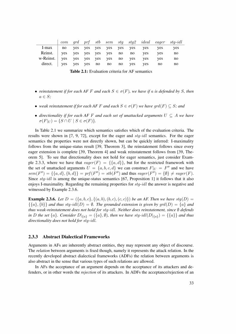
com grd prf stb sem stg stg2 ideal eager stg-idlI-max no yes yes yes yes yes yes yes yes yesReinst. yes yes yes yes yes no no yes yes no

w-Reinst. yes yes yes yes yes no yes yes yes nodirect. yes yes yes no no no yes yes no no

Table 2.1: Evaluation criteria for AF semantics

• reinstatement if for each AF F and each S ∈ σ(F ), we have if a is defended by S, thena ∈ S;

• weak reinstatement if for each AF F and each S ∈ σ(F ) we have grd(F ) ⊆ S; and

• directionality if for each AF F and each set of unattacked arguments U ⊆ A we haveσ(F |U ) = {S ∩ U | S ∈ σ(F )}.

In Table 2.1 we summarize which semantics satisfies which of the evaluation criteria. Theresults were shown in [7, 9, 72], except for the eager and stg-idl semantics. For the eagersemantics the properties were not directly shown, but can be quickly inferred: I-maximalityfollows from the unique-status result [39, Theorem 3], the reinstatement follows since everyeager extension is complete [39, Theorem 4] and weak reinstatement follows from [39, The-orem 5]. To see that directionality does not hold for eager semantics, just consider Exam-ple 2.3.3, where we have that eager(F ) = {{a, d}}, but for the restricted framework withthe set of unattacked arguments U = {a, b, c, d} we can construct F |U = F ′′ and we havesem(F ′′) = {{a, d}, {b, d}} = prf (F ′′) = stb(F ′′) and thus eager(F ′′) = {∅} 6= eager(F ).Since stg-idl is among the unique-status semantics [67, Proposition 1] it follows that it alsoenjoys I-maximality. Regarding the remaining properties for stg-idl the answer is negative andwitnessed by Example 2.3.6.

Example 2.3.6. Let D = ({a, b, c}, {(a, b), (b, c), (c, c)}) be an AF. Then we have stg(D) ={{a}, {b}} and thus stg-idl(D) = ∅. The grounded extension is given by grd(D) = {a} andthus weak-reinstatement does not hold for stg-idl . Neither does reinstatement, since ∅ defendsin D the set {a}. Consider D|{a} = ({a}, ∅), then we have stg-idl(D|{a}) = {{a}} and thusdirectionality does not hold for stg-idl .

2.3.3 Abstract Dialectical Frameworks

Arguments in AFs are inherently abstract entities, they may represent any object of discourse.The relation between arguments is fixed though, namely it represents the attack relation. In therecently developed abstract dialectical frameworks (ADFs) the relation between arguments isalso abstract in the sense that various types of such relations are allowed.

In AFs the acceptance of an argument depends on the acceptance of its attackers and de-fenders, or in other words the rejection of its attackers. In ADFs the acceptance/rejection of an

33

argument s likewise depends on the status of a set of arguments, here called the parents anddenoted by par(s), but instead of specifying that s is acceptable if all its parents are rejected,in ADFs any combination of accepted/rejected parents may lead to acceptance of s. This leadsto the notion of an acceptance condition, which relates the status of the parents of an argumentto either acceptance or rejection. Again as for argumentation frameworks we take our set ofarguments from P .

Definition 2.3.19. An abstract dialectical framework (ADF) is a tuple (S,L,C), where

• S ⊆ P is a set of abstract arguments,

• L ⊆ S × S is a set of links and

• C = {Cs}s∈S is a set of functions Cs : 2par(s) → {t, f}. Cs is called acceptancecondition of s.

We denote by ADFP the set of all ADFs over P .

The set of parents is defined via the links: par(s) = {x ∈ S | (x, s) ∈ L}. The links L areabstract links, denoting some relation, but not restricted to a particular one. Originally the ac-ceptance conditions returned in or out, but we chose in this thesis the truth value style, since weoften translate problems of argumentation to propositional logic and vice versa. An acceptancecondition not only closely resembles a Boolean function, i.e. returning v ∈ {t, f} for a subsetof par(s), we can straightforwardly define each acceptance condition as a Boolean formula. Weusually denote by Cs the acceptance condition as the Boolean function and by ϕs the acceptancecondition as a Boolean formula, s.t. forX ⊆ S we haveCs(X∩par(s)) = t iffX |= ϕs, i.e. theacceptance condition evaluates to true under X ∩ par(s) iff the acceptance formula evaluates totrue under X . It is immediate that any such function for an acceptance condition can be writtenequivalently as a Boolean formula. For a closer study on these two forms the interested reader isreferred to [89]. Unless noted otherwise we will assume that only the propositional formulae foreach argument are given for an ADF. The difference in use of the two forms may be particularlyimportant for computational purposes, since a naive representation of the Boolean function Csconsists of specifying the result for all subsets of par(s), while the corresponding formula ϕsmaybe much more compact, in fact the naive representation may be exponentially larger thanthe formula.

While the acceptance conditions specify the exact condition when we may accept an argu-ment, the links are used to show dependencies between the arguments. For an argument s andthe acceptance conditions as Boolean formulae we can see the set of parents of s by lookingat atoms(ϕs) = par(s). In principle one could define ADFs without links, e.g. just using aset of arguments and one formula for each argument as its acceptance condition, since the linkscan be extracted via the atoms function. So it would be sufficient to write ADFs as a pairD = (S,C). We however stick to the definition with triples, but will not always define the setof links explicitly, assuming that they are defined implicitly via the acceptance conditions.

Since the occurrence of an argument in atoms(ϕs) respectively in par(s) does not imply aparticular relation between s and the parent, as was the case in AFs, we distinguish in the contextof ADFs four different classes of relations [34]. A link can be of an attacking, a supporting or

34

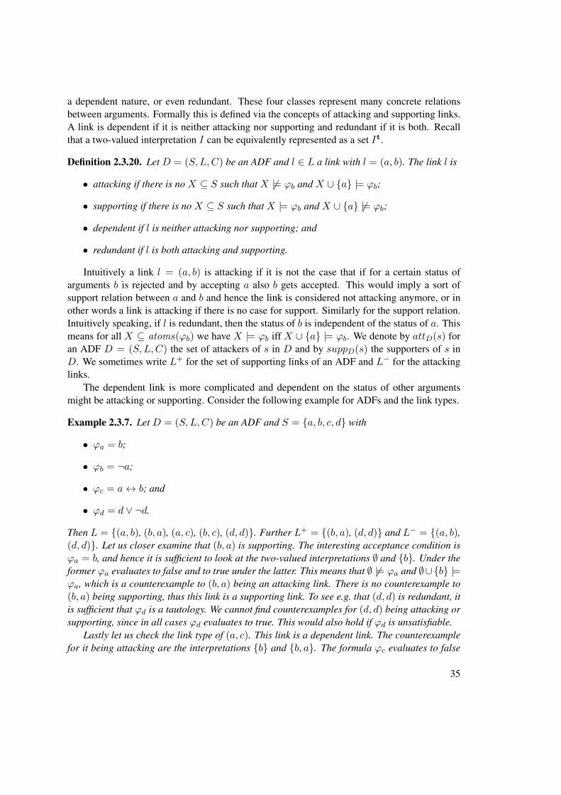
a dependent nature, or even redundant. These four classes represent many concrete relationsbetween arguments. Formally this is defined via the concepts of attacking and supporting links.A link is dependent if it is neither attacking nor supporting and redundant if it is both. Recallthat a two-valued interpretation I can be equivalently represented as a set It.

Definition 2.3.20. Let D = (S,L,C) be an ADF and l ∈ L a link with l = (a, b). The link l is

• attacking if there is no X ⊆ S such that X 6|= ϕb and X ∪ {a} |= ϕb;

• supporting if there is no X ⊆ S such that X |= ϕb and X ∪ {a} 6|= ϕb;

• dependent if l is neither attacking nor supporting; and

• redundant if l is both attacking and supporting.

Intuitively a link l = (a, b) is attacking if it is not the case that if for a certain status ofarguments b is rejected and by accepting a also b gets accepted. This would imply a sort ofsupport relation between a and b and hence the link is considered not attacking anymore, or inother words a link is attacking if there is no case for support. Similarly for the support relation.Intuitively speaking, if l is redundant, then the status of b is independent of the status of a. Thismeans for all X ⊆ atoms(ϕb) we have X |= ϕb iff X ∪ {a} |= ϕb. We denote by attD(s) foran ADF D = (S,L,C) the set of attackers of s in D and by suppD(s) the supporters of s inD. We sometimes write L+ for the set of supporting links of an ADF and L− for the attackinglinks.

The dependent link is more complicated and dependent on the status of other argumentsmight be attacking or supporting. Consider the following example for ADFs and the link types.

Example 2.3.7. Let D = (S,L,C) be an ADF and S = {a, b, c, d} with

• ϕa = b;

• ϕb = ¬a;

• ϕc = a↔ b; and

• ϕd = d ∨ ¬d.

Then L = {(a, b), (b, a), (a, c), (b, c), (d, d)}. Further L+ = {(b, a), (d, d)} and L− = {(a, b),(d, d)}. Let us closer examine that (b, a) is supporting. The interesting acceptance condition isϕa = b, and hence it is sufficient to look at the two-valued interpretations ∅ and {b}. Under theformer ϕa evaluates to false and to true under the latter. This means that ∅ 6|= ϕa and ∅∪{b} |=ϕa, which is a counterexample to (b, a) being an attacking link. There is no counterexample to(b, a) being supporting, thus this link is a supporting link. To see e.g. that (d, d) is redundant, itis sufficient that ϕd is a tautology. We cannot find counterexamples for (d, d) being attacking orsupporting, since in all cases ϕd evaluates to true. This would also hold if ϕd is unsatisfiable.

Lastly let us check the link type of (a, c). This link is a dependent link. The counterexamplefor it being attacking are the interpretations {b} and {b, a}. The formula ϕc evaluates to false

35

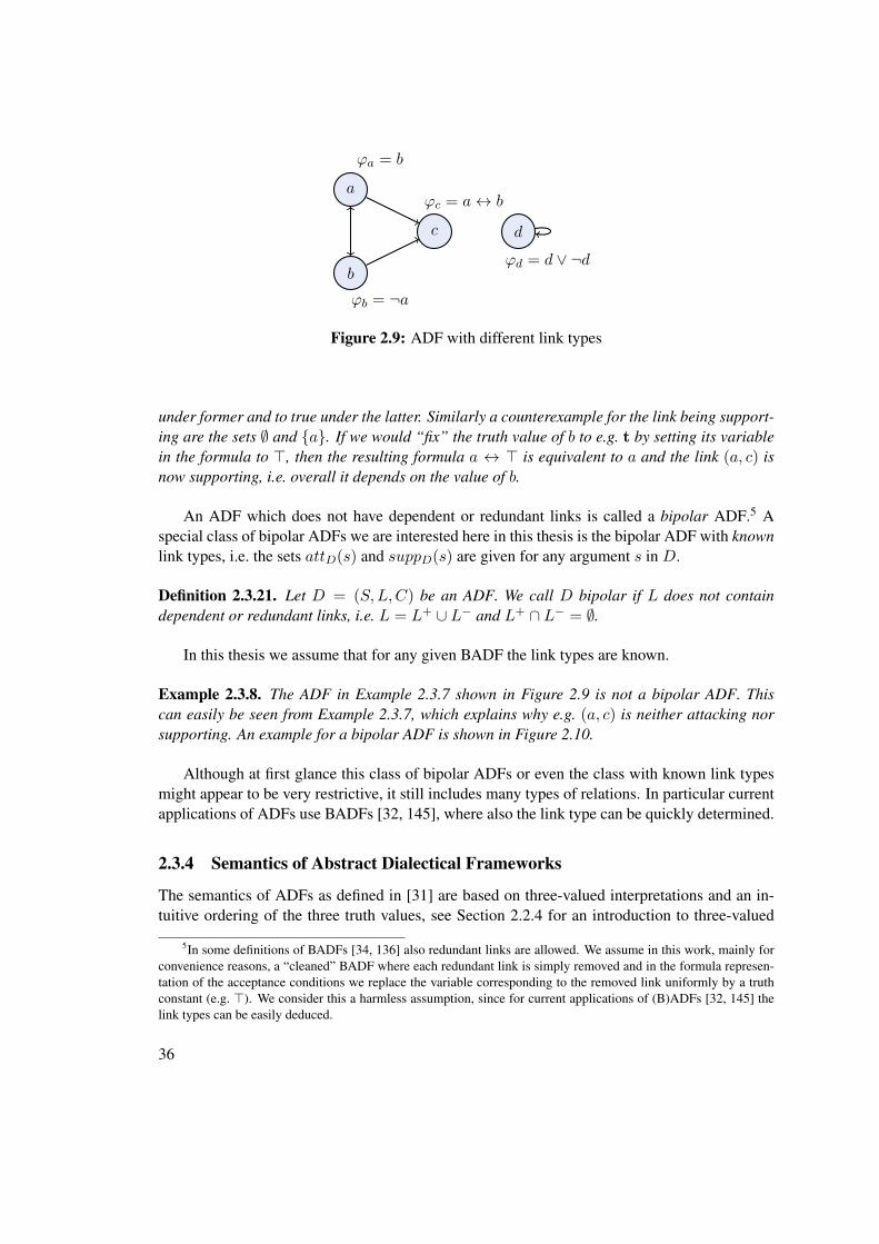
a

ϕa = b

b

ϕb = ¬a

c

ϕc = a↔ b

d

ϕd = d ∨ ¬d

Figure 2.9: ADF with different link types

under former and to true under the latter. Similarly a counterexample for the link being support-ing are the sets ∅ and {a}. If we would “fix” the truth value of b to e.g. t by setting its variablein the formula to >, then the resulting formula a ↔ > is equivalent to a and the link (a, c) isnow supporting, i.e. overall it depends on the value of b.

An ADF which does not have dependent or redundant links is called a bipolar ADF.5 Aspecial class of bipolar ADFs we are interested here in this thesis is the bipolar ADF with knownlink types, i.e. the sets attD(s) and suppD(s) are given for any argument s in D.

Definition 2.3.21. Let D = (S,L,C) be an ADF. We call D bipolar if L does not containdependent or redundant links, i.e. L = L+ ∪ L− and L+ ∩ L− = ∅.

In this thesis we assume that for any given BADF the link types are known.

Example 2.3.8. The ADF in Example 2.3.7 shown in Figure 2.9 is not a bipolar ADF. Thiscan easily be seen from Example 2.3.7, which explains why e.g. (a, c) is neither attacking norsupporting. An example for a bipolar ADF is shown in Figure 2.10.

Although at first glance this class of bipolar ADFs or even the class with known link typesmight appear to be very restrictive, it still includes many types of relations. In particular currentapplications of ADFs use BADFs [32, 145], where also the link type can be quickly determined.

2.3.4 Semantics of Abstract Dialectical Frameworks

The semantics of ADFs as defined in [31] are based on three-valued interpretations and an in-tuitive ordering of the three truth values, see Section 2.2.4 for an introduction to three-valued

5In some definitions of BADFs [34, 136] also redundant links are allowed. We assume in this work, mainly forconvenience reasons, a “cleaned” BADF where each redundant link is simply removed and in the formula represen-tation of the acceptance conditions we replace the variable corresponding to the removed link uniformly by a truthconstant (e.g. >). We consider this a harmless assumption, since for current applications of (B)ADFs [32, 145] thelink types can be easily deduced.

36

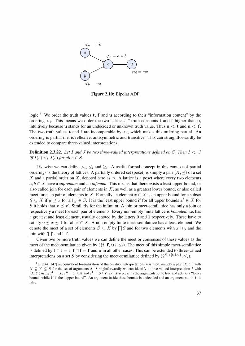
a

ϕa = ¬b

b

ϕb = ¬a

c

ϕc = a ∨ bd

ϕd = ¬c

Figure 2.10: Bipolar ADF

logic.6 We order the truth values t, f and u according to their “information content” by theordering <i. This means we order the two “classical” truth constants t and f higher than u,intuitively because u stands for an undecided or unknown truth value. Thus u <i t and u <i f .The two truth values t and f are incomparable by <i, which makes this ordering partial. Anordering is partial if it is reflexive, antisymmetric and transitive. This can straightforwardly beextended to compare three-valued interpretations.

Definition 2.3.22. Let I and J be two three-valued interpretations defined on S. Then I <i Jiff I(s) <i J(s) for all s ∈ S.

Likewise we can define >i, ≤i and ≥i. A useful formal concept in this context of partialorderings is the theory of lattices. A partially ordered set (poset) is simply a pair (X,�) of a setX and a partial order on X , denoted here as �. A lattice is a poset where every two elementsa, b ∈ X have a supremum and an infimum. This means that there exists a least upper bound, oralso called join for each pair of elements in X , as well as a greatest lower bound, or also calledmeet for each pair of elements in X . Formally an element x ∈ X is an upper bound for a subsetS ⊆ X if y � x for all y ∈ S. It is the least upper bound if for all upper bounds x′ ∈ X forS it holds that x � x′. Similarly for the infimum. A join or meet-semilattice has only a join orrespectively a meet for each pair of elements. Every non-empty finite lattice is bounded, i.e. hasa greatest and least element, usually denoted by the letters 0 and 1 respectively. These have tosatisfy 0 � x � 1 for all x ∈ X . A non-empty finite meet-semilattice has a least element. Wedenote the meet of a set of elements S ⊆ X by

dS and for two elements with x u y and the

join with ’⊔

’ and ’t’.Given two or more truth values we can define the meet or consensus of these values as the

meet of the meet-semilattice given by ({t, f , u},≤i). The meet of this simple meet-semilatticeis defined by t u t = t, f u f = f and u in all other cases. This can be extended to three-valuedinterpretations on a set S by considering the meet-semilattice defined by (2S→{t,f ,u},≤i).

6In [144, 147] an equivalent formalization of three-valued interpretations was used, namely a pair (X,Y ) withX ⊆ Y ⊆ S for the set of arguments S. Straightforwardly we can identify a three-valued interpretation I with(X,Y ) using It = X , Iu = Y \X and If = S \ Y , i.e. X represents the arguments set to true and acts as a “lowerbound” while Y is the “upper bound”. An argument inside these bounds is undecided and an argument not in Y isfalse.

37

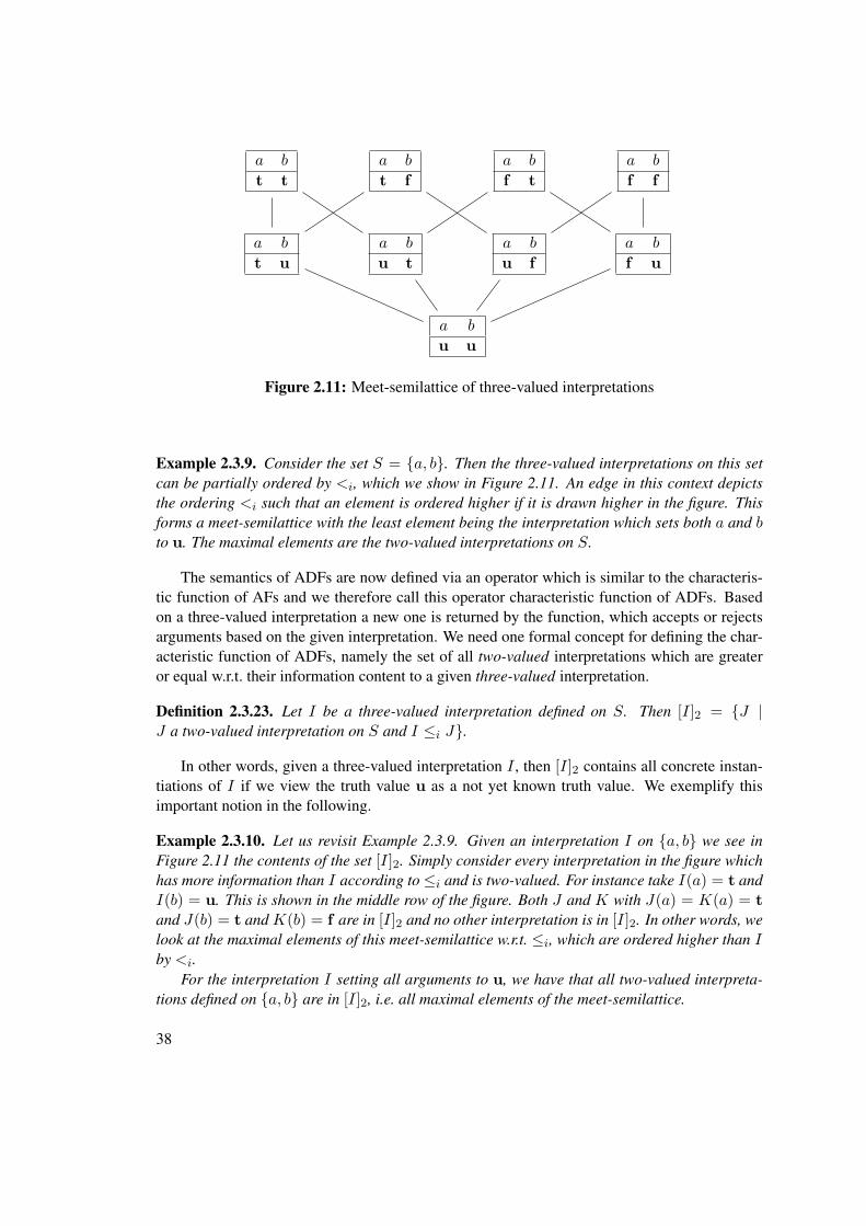
a b

u u

a b

t u

a b

u t

a b

f u

a b

u f

a b

t t

a b

t f

a b

f t

a b

f f

Figure 2.11: Meet-semilattice of three-valued interpretations

Example 2.3.9. Consider the set S = {a, b}. Then the three-valued interpretations on this setcan be partially ordered by <i, which we show in Figure 2.11. An edge in this context depictsthe ordering <i such that an element is ordered higher if it is drawn higher in the figure. Thisforms a meet-semilattice with the least element being the interpretation which sets both a and bto u. The maximal elements are the two-valued interpretations on S.

The semantics of ADFs are now defined via an operator which is similar to the characteris-tic function of AFs and we therefore call this operator characteristic function of ADFs. Basedon a three-valued interpretation a new one is returned by the function, which accepts or rejectsarguments based on the given interpretation. We need one formal concept for defining the char-acteristic function of ADFs, namely the set of all two-valued interpretations which are greateror equal w.r.t. their information content to a given three-valued interpretation.

Definition 2.3.23. Let I be a three-valued interpretation defined on S. Then [I]2 = {J |J a two-valued interpretation on S and I ≤i J}.

In other words, given a three-valued interpretation I , then [I]2 contains all concrete instan-tiations of I if we view the truth value u as a not yet known truth value. We exemplify thisimportant notion in the following.

Example 2.3.10. Let us revisit Example 2.3.9. Given an interpretation I on {a, b} we see inFigure 2.11 the contents of the set [I]2. Simply consider every interpretation in the figure whichhas more information than I according to≤i and is two-valued. For instance take I(a) = t andI(b) = u. This is shown in the middle row of the figure. Both J and K with J(a) = K(a) = tand J(b) = t and K(b) = f are in [I]2 and no other interpretation is in [I]2. In other words, welook at the maximal elements of this meet-semilattice w.r.t. ≤i, which are ordered higher than Iby <i.

For the interpretation I setting all arguments to u, we have that all two-valued interpreta-tions defined on {a, b} are in [I]2, i.e. all maximal elements of the meet-semilattice.

38

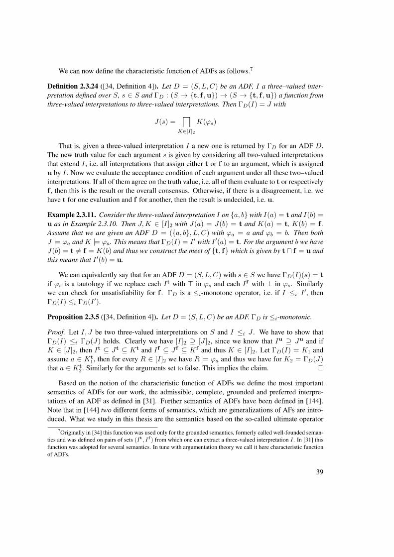
We can now define the characteristic function of ADFs as follows.7

Definition 2.3.24 ([34, Definition 4]). Let D = (S,L,C) be an ADF, I a three–valued inter-pretation defined over S, s ∈ S and ΓD : (S → {t, f ,u}) → (S → {t, f ,u}) a function fromthree-valued interpretations to three-valued interpretations. Then ΓD(I) = J with

J(s) =l

K∈[I]2

K(ϕs)

That is, given a three-valued interpretation I a new one is returned by ΓD for an ADF D.The new truth value for each argument s is given by considering all two-valued interpretationsthat extend I , i.e. all interpretations that assign either t or f to an argument, which is assignedu by I . Now we evaluate the acceptance condition of each argument under all these two–valuedinterpretations. If all of them agree on the truth value, i.e. all of them evaluate to t or respectivelyf , then this is the result or the overall consensus. Otherwise, if there is a disagreement, i.e. wehave t for one evaluation and f for another, then the result is undecided, i.e. u.

Example 2.3.11. Consider the three-valued interpretation I on {a, b} with I(a) = t and I(b) =u as in Example 2.3.10. Then J,K ∈ [I]2 with J(a) = J(b) = t and K(a) = t, K(b) = f .Assume that we are given an ADF D = ({a, b}, L, C) with ϕa = a and ϕb = b. Then bothJ |= ϕa and K |= ϕa. This means that ΓD(I) = I ′ with I ′(a) = t. For the argument b we haveJ(b) = t 6= f = K(b) and thus we construct the meet of {t, f} which is given by t u f = u andthis means that I ′(b) = u.

We can equivalently say that for an ADF D = (S,L,C) with s ∈ S we have ΓD(I)(s) = tif ϕs is a tautology if we replace each It with > in ϕs and each If with ⊥ in ϕs. Similarlywe can check for unsatisfiability for f . ΓD is a ≤i-monotone operator, i.e. if I ≤i I ′, thenΓD(I) ≤i ΓD(I ′).

Proposition 2.3.5 ([34, Definition 4]). Let D = (S,L,C) be an ADF. ΓD is ≤i-monotonic.

Proof. Let I, J be two three-valued interpretations on S and I ≤i J . We have to show thatΓD(I) ≤i ΓD(J) holds. Clearly we have [I]2 ⊇ [J ]2, since we know that Iu ⊇ Ju and ifK ∈ [J ]2, then It ⊆ Jt ⊆ Kt and If ⊆ J f ⊆ Kf and thus K ∈ [I]2. Let ΓD(I) = K1 andassume a ∈ Kt

1 , then for every R ∈ [I]2 we have R |= ϕa and thus we have for K2 = ΓD(J)that a ∈ Kt

2 . Similarly for the arguments set to false. This implies the claim.

Based on the notion of the characteristic function of ADFs we define the most importantsemantics of ADFs for our work, the admissible, complete, grounded and preferred interpre-tations of an ADF as defined in [31]. Further semantics of ADFs have been defined in [144].Note that in [144] two different forms of semantics, which are generalizations of AFs are intro-duced. What we study in this thesis are the semantics based on the so-called ultimate operator

7Originally in [34] this function was used only for the grounded semantics, formerly called well-founded seman-tics and was defined on pairs of sets (It, If ) from which one can extract a three-valued interpretation I . In [31] thisfunction was adopted for several semantics. In tune with argumentation theory we call it here characteristic functionof ADFs.

39

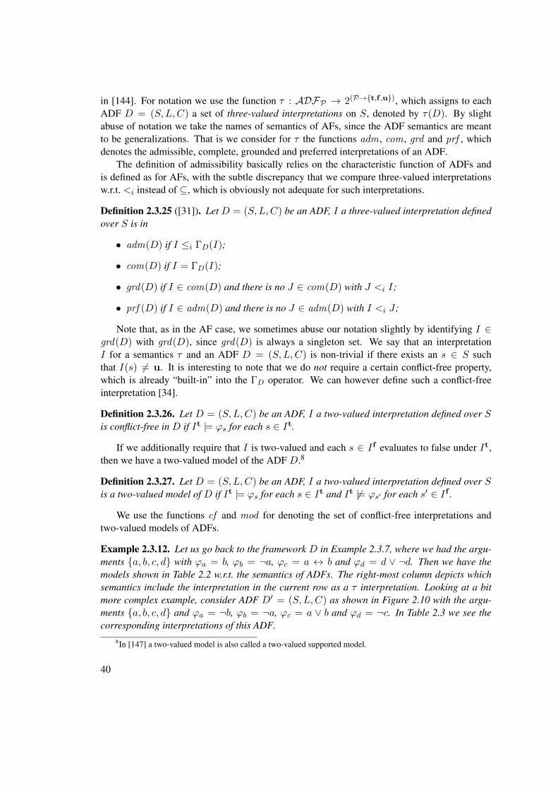
in [144]. For notation we use the function τ : ADFP → 2(P→{t,f ,u}), which assigns to eachADF D = (S,L,C) a set of three-valued interpretations on S, denoted by τ(D). By slightabuse of notation we take the names of semantics of AFs, since the ADF semantics are meantto be generalizations. That is we consider for τ the functions adm , com , grd and prf , whichdenotes the admissible, complete, grounded and preferred interpretations of an ADF.

The definition of admissibility basically relies on the characteristic function of ADFs andis defined as for AFs, with the subtle discrepancy that we compare three-valued interpretationsw.r.t. <i instead of ⊆, which is obviously not adequate for such interpretations.

Definition 2.3.25 ([31]). Let D = (S,L,C) be an ADF, I a three-valued interpretation definedover S is in

• adm(D) if I ≤i ΓD(I);

• com(D) if I = ΓD(I);

• grd(D) if I ∈ com(D) and there is no J ∈ com(D) with J <i I;

• prf (D) if I ∈ adm(D) and there is no J ∈ adm(D) with I <i J;

Note that, as in the AF case, we sometimes abuse our notation slightly by identifying I ∈grd(D) with grd(D), since grd(D) is always a singleton set. We say that an interpretationI for a semantics τ and an ADF D = (S,L,C) is non-trivial if there exists an s ∈ S suchthat I(s) 6= u. It is interesting to note that we do not require a certain conflict-free property,which is already “built-in” into the ΓD operator. We can however define such a conflict-freeinterpretation [34].

Definition 2.3.26. Let D = (S,L,C) be an ADF, I a two-valued interpretation defined over Sis conflict-free in D if It |= ϕs for each s ∈ It.

If we additionally require that I is two-valued and each s ∈ If evaluates to false under It,then we have a two-valued model of the ADF D.8

Definition 2.3.27. Let D = (S,L,C) be an ADF, I a two-valued interpretation defined over Sis a two-valued model of D if It |= ϕs for each s ∈ It and It 6|= ϕs′ for each s′ ∈ If .

We use the functions cf and mod for denoting the set of conflict-free interpretations andtwo-valued models of ADFs.

Example 2.3.12. Let us go back to the framework D in Example 2.3.7, where we had the argu-ments {a, b, c, d} with ϕa = b, ϕb = ¬a, ϕc = a ↔ b and ϕd = d ∨ ¬d. Then we have themodels shown in Table 2.2 w.r.t. the semantics of ADFs. The right-most column depicts whichsemantics include the interpretation in the current row as a τ interpretation. Looking at a bitmore complex example, consider ADF D′ = (S,L,C) as shown in Figure 2.10 with the argu-ments {a, b, c, d} and ϕa = ¬b, ϕb = ¬a, ϕc = a ∨ b and ϕd = ¬c. In Table 2.3 we see thecorresponding interpretations of this ADF.

8In [147] a two-valued model is also called a two-valued supported model.

40

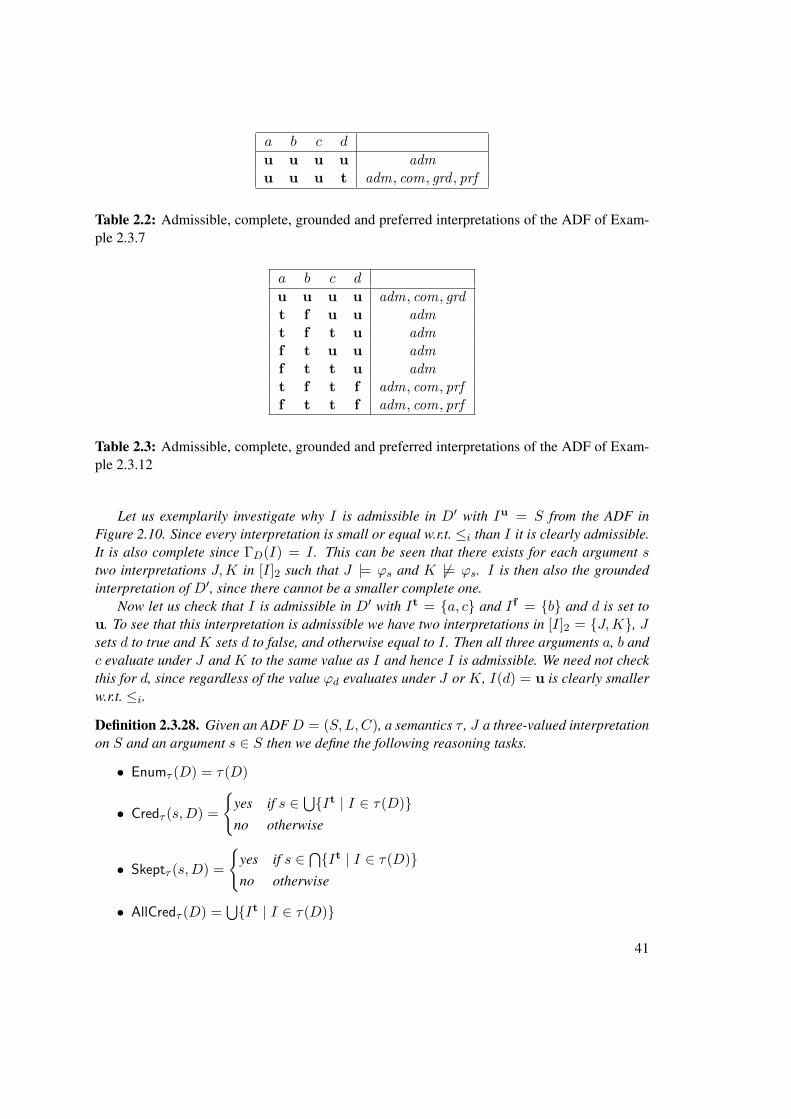
a b c d

u u u u admu u u t adm, com, grd , prf

Table 2.2: Admissible, complete, grounded and preferred interpretations of the ADF of Exam-ple 2.3.7

a b c d

u u u u adm, com, grdt f u u admt f t u admf t u u admf t t u admt f t f adm, com, prff t t f adm, com, prf

Table 2.3: Admissible, complete, grounded and preferred interpretations of the ADF of Exam-ple 2.3.12

Let us exemplarily investigate why I is admissible in D′ with Iu = S from the ADF inFigure 2.10. Since every interpretation is small or equal w.r.t. ≤i than I it is clearly admissible.It is also complete since ΓD(I) = I . This can be seen that there exists for each argument stwo interpretations J,K in [I]2 such that J |= ϕs and K 6|= ϕs. I is then also the groundedinterpretation of D′, since there cannot be a smaller complete one.

Now let us check that I is admissible in D′ with It = {a, c} and If = {b} and d is set tou. To see that this interpretation is admissible we have two interpretations in [I]2 = {J,K}, Jsets d to true and K sets d to false, and otherwise equal to I . Then all three arguments a, b andc evaluate under J and K to the same value as I and hence I is admissible. We need not checkthis for d, since regardless of the value ϕd evaluates under J or K, I(d) = u is clearly smallerw.r.t. ≤i.

Definition 2.3.28. Given an ADFD = (S,L,C), a semantics τ , J a three-valued interpretationon S and an argument s ∈ S then we define the following reasoning tasks.

• Enumτ (D) = τ(D)

• Credτ (s,D) =

{yes if s ∈ ⋃{It | I ∈ τ(D)}no otherwise

• Skeptτ (s,D) =

{yes if s ∈ ⋂{It | I ∈ τ(D)}no otherwise

• AllCredτ (D) =⋃{It | I ∈ τ(D)}

41

• AllSkeptτ (D) =⋂{It | I ∈ τ(D)}

• Verτ (J,D) =

{yes if J ∈ τ(D)

no otherwise

Example 2.3.13. Consider the ADF D′ of Example 2.3.12. Then Credadm(a,D′) = yes andSkeptprf (d,D′) = no.

We now show some basic properties of ADFs. First due to [54, Theorem 8.22] (a variant ofthe Knaster-Tarski Theorem applicable for our current setting) we know that for any ADF thereexists a grounded interpretation and thus also at least one complete pair.9 Similarly as in AFsone has a strong relation between the semantics defined on ADFs. Every two-valued model is apreferred interpretations of an ADF. Every preferred interpretation is a complete one and in turnis also admissible.

Theorem 2.3.6 ([31, Theorem 2]). LetD = (S,L,C) be an ADF. Then the following inclusionshold: mod(D) ⊆ prf (D) ⊆ com(D) ⊆ adm(D). If I ∈ adm(D), then It ∈ cf (D).

Proof. The three inclusions were proven in [31, Theorem 2]. To show that if I is an admissibleinterpretation then It is also conflict-free just observe that It ∈ [I], i.e. the two-valued inter-pretation It is in [I]2. Since for every J ∈ [I]2 we have that J |= ϕa for a ∈ It (since I isadmissible), the claim follows.

The relations between the ADF semantics are shown in Figure 2.12. An arrow from τ1 to τ2

denotes that for any ADFD we have τ1(D) ⊆ τ2(D). The dotted line indicates that if I ∈ τ1(D)then It ∈ τ2(D).

Definition 2.3.29. Let F = (A,R) be an AF. Then its associated ADF DF = (A,R,C) isdefined by ϕs =

∧(a,s)∈R ¬a for each s ∈ A.

The associated ADF for an AF is clearly bipolar, it actually only includes attacking links.

Example 2.3.14. Consider the AF from Example 2.3.1. We show in Figure 2.13 the associatedADF of this AF.

The correspondence between the semantics of an AF and its associated ADF can now beshown.10

Theorem 2.3.7 ([31, Theorem 2 and Theorem 4] and [34, Proposition 1]). Let F be an AF andits associated ADF be DF . Then

9In [31] the grounded semantics was defined as the least fixed point of ΓD for an ADF D. Due to [54, Theorem8.22] we know that there exists such a least fixed point and hence complete interpretations with a particular completeinterpretation being the least one w.r.t. ≤i. Thus we can equivalently define the grounded interpretation as the leastfixed point of ΓD or the least complete interpretation w.r.t. ≤i of an ADF.

10Another generalization of the AF stable semantics is the ADF stable semantics [31, 147], however for an ADFassociated with an AF two-valued models and two-valued stable models coincide, since, intuitively speaking, AFsdo not feature a support relation.

42

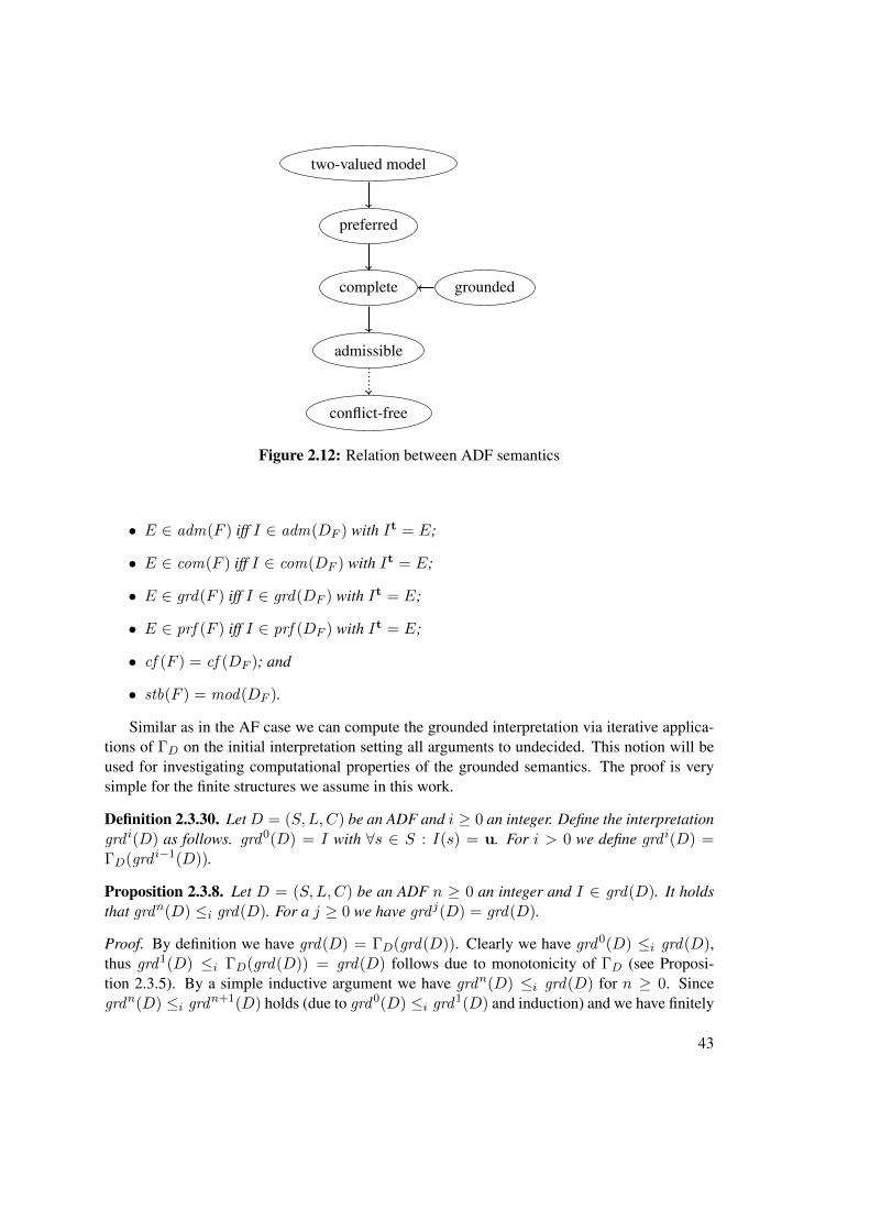
two-valued model

preferred

complete

admissible

grounded

conflict-free

Figure 2.12: Relation between ADF semantics

• E ∈ adm(F ) iff I ∈ adm(DF ) with It = E;

• E ∈ com(F ) iff I ∈ com(DF ) with It = E;

• E ∈ grd(F ) iff I ∈ grd(DF ) with It = E;

• E ∈ prf (F ) iff I ∈ prf (DF ) with It = E;

• cf (F ) = cf (DF ); and

• stb(F ) = mod(DF ).

Similar as in the AF case we can compute the grounded interpretation via iterative applica-tions of ΓD on the initial interpretation setting all arguments to undecided. This notion will beused for investigating computational properties of the grounded semantics. The proof is verysimple for the finite structures we assume in this work.

Definition 2.3.30. LetD = (S,L,C) be an ADF and i ≥ 0 an integer. Define the interpretationgrd i(D) as follows. grd0(D) = I with ∀s ∈ S : I(s) = u. For i > 0 we define grd i(D) =ΓD(grd i−1(D)).

Proposition 2.3.8. Let D = (S,L,C) be an ADF n ≥ 0 an integer and I ∈ grd(D). It holdsthat grdn(D) ≤i grd(D). For a j ≥ 0 we have grd j(D) = grd(D).

Proof. By definition we have grd(D) = ΓD(grd(D)). Clearly we have grd0(D) ≤i grd(D),thus grd1(D) ≤i ΓD(grd(D)) = grd(D) follows due to monotonicity of ΓD (see Proposi-tion 2.3.5). By a simple inductive argument we have grdn(D) ≤i grd(D) for n ≥ 0. Sincegrdn(D) ≤i grdn+1(D) holds (due to grd0(D) ≤i grd1(D) and induction) and we have finitely

43

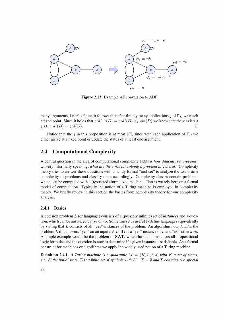
a

b

c d

e

a ϕa = ¬b

b

ϕb = ¬a

c

ϕc = ¬a ∧ ¬bd

ϕd = ¬c

e

ϕe = ¬a ∧ ¬e

Figure 2.13: Example AF conversion to ADF

many arguments, i.e. S is finite, it follows that after finitely many applications j of ΓD we reacha fixed point. Since it holds that grd j+1(D) = grd j(D) ≤i grd(D) we know that there exists aj s.t. grd j(D) = grd(D).

Notice that the j in this proposition is at most |S|, since with each application of ΓD weeither arrive at a fixed point or update the status of at least one argument.

2.4 Computational Complexity

A central question in the area of computational complexity [133] is how difficult is a problem?Or very informally speaking, what are the costs for solving a problem in general? Complexitytheory tries to answer these questions with a handy formal “tool set” to analyze the worst-timecomplexity of problems and classify them accordingly. Complexity classes contain problemswhich can be computed with a (restricted) formalized machine. That is we rely here on a formalmodel of computation. Typically the notion of a Turing machine is employed in complexitytheory. We briefly review in this section the basics from complexity theory for our complexityanalysis.

2.4.1 Basics

A decision problem L (or language) consists of a (possibly infinite) set of instances and a ques-tion, which can be answered by yes or no. Sometimes it is useful to define languages equivalentlyby stating that L consists of all “yes”-instances of the problem. An algorithm now decides theproblem L if it answers “yes” on an input l ∈ L iff l is a “yes” instance of L and “no” otherwise.A simple example would be the problem of SAT, which has as its instances all propositionallogic formulae and the question is now to determine if a given instance is satisfiable. As a formalconstruct for machines or algorithms we apply the widely used notion of a Turing machine.

Definition 2.4.1. A Turing machine is a quadruple M = (K,Σ, δ, s) with K a set of states,s ∈ K the initial state. Σ is a finite set of symbols with K ∩ Σ = ∅ and Σ contains two special

44

symbols, the blank and first symbols {t,B} ⊆ Σ. We assume that h (the halting state), “yes”,“no” and the cursor directions ’←−’, ’−→’ as well as ’−’ are not present in K ∪ Σ. Finally,

• M is a deterministic Turing machine if δ is a transition function

δ : K × Σ→ (K ∪ {h,“yes”,“no”})× Σ× {←−,−→,−}

• M is a non-deterministic Turing machine if δ is a transition relation

δ ⊂ K × Σ× (K ∪ {h,“yes”,“no”})× Σ× {←−,−→,−}

Informally speaking, a Turing machine is a description of an algorithm which works in thefollowing way. The machine starts in the initial state s and has a “tape” where it reads andwrites. This tape starts with the input to our algorithm/Turing machine. The symbols on thetape may be taken from Σ. The special symbols denote the start symbol B, which just statesthat this is the beginning of the tape and special empty symbols t. Usually one assumes that theword initially given terminates with a blank symbol (or infinitely many of them at the right side).The transition function or relation now defines the algorithm, i.e. what the machine should do inwhich situation. A transition function takes as input the current state, the symbol the machinereads and outputs a new state (possibly the same), a new symbol which should be written insteadof the current one (possibly the same) and a direction to “move” the reader, i.e. which symbolshould be read next, the one left or right from the current position (denoted by←− and −→) orshould it stay in the current position (using −).

In case of a non-deterministic Turing machine we may have a choice for the next state, i.e.it is non-deterministic in the sense that given a current state and a read symbol we may haveseveral options. Note that the transition relation may be a function, i.e. assigning to each pairof state and symbol exactly one choice. This immediately implies that non-deterministic Turingmachines are a generalization of deterministic ones. We now define what it means to “compute”using a Turing machine.

Definition 2.4.2. Let M be a deterministic Turing machine. A configuration is a triple (q, w, u)with q ∈ K and w, u ∈ Σ∗. We say that for this configuration q is the current state, w isthe string left of the cursor including the cursor position and u right of the cursor. W.r.t. M aconfiguration (q, w, u) yields in one step a configuration (q′, w′, u′), denoted by (q, w, u)

M−→(q′, w′, u′), if i is the last symbol of w and δ(q, i) = (p, ρ,D) with q′ = p and depending on Done of three cases is true.

• if D =−→ then w′ is w with the last symbol i replaced by ρ and the first symbol of uappended to it (t if u was empty) and u′ is u with the first symbol removed (or t if u wasempty);

• if D =←− then w′ is w with the last symbol i omitted from its end, and u′ is u with ρattached in the beginning;

• if D = − then w′ is w with the ending i replaced by ρ and u′ = u.

45

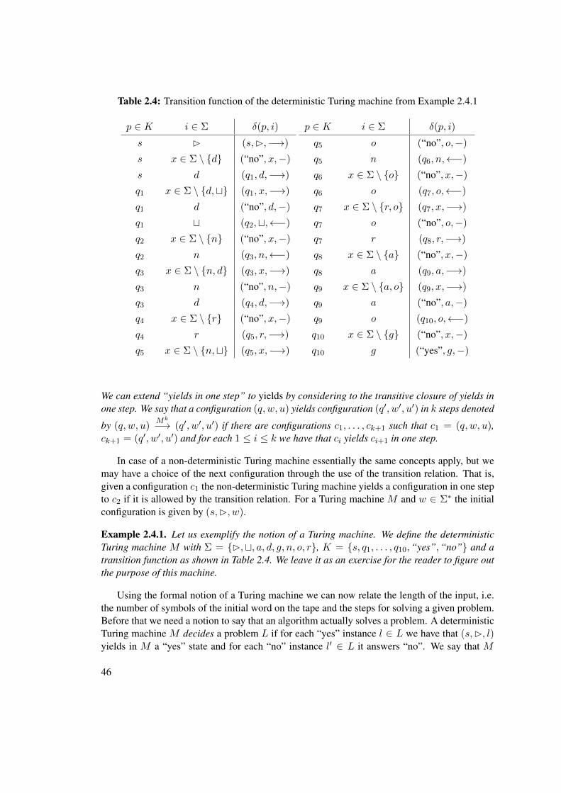
Table 2.4: Transition function of the deterministic Turing machine from Example 2.4.1

p ∈ K i ∈ Σ δ(p, i)

s B (s,B,−→)

s x ∈ Σ \ {d} (“no”, x,−)

s d (q1, d,−→)

q1 x ∈ Σ \ {d,t} (q1, x,−→)

q1 d (“no”, d,−)

q1 t (q2,t,←−)

q2 x ∈ Σ \ {n} (“no”, x,−)

q2 n (q3, n,←−)

q3 x ∈ Σ \ {n, d} (q3, x,−→)

q3 n (“no”, n,−)

q3 d (q4, d,−→)

q4 x ∈ Σ \ {r} (“no”, x,−)

q4 r (q5, r,−→)

q5 x ∈ Σ \ {n,t} (q5, x,−→)

p ∈ K i ∈ Σ δ(p, i)

q5 o (“no”, o,−)

q5 n (q6, n,←−)

q6 x ∈ Σ \ {o} (“no”, x,−)

q6 o (q7, o,←−)

q7 x ∈ Σ \ {r, o} (q7, x,−→)

q7 o (“no”, o,−)

q7 r (q8, r,−→)

q8 x ∈ Σ \ {a} (“no”, x,−)

q8 a (q9, a,−→)

q9 x ∈ Σ \ {a, o} (q9, x,−→)

q9 a (“no”, a,−)

q9 o (q10, o,←−)

q10 x ∈ Σ \ {g} (“no”, x,−)

q10 g (“yes”, g,−)

We can extend “yields in one step” to yields by considering to the transitive closure of yields inone step. We say that a configuration (q, w, u) yields configuration (q′, w′, u′) in k steps denoted

by (q, w, u)Mk

−→ (q′, w′, u′) if there are configurations c1, . . . , ck+1 such that c1 = (q, w, u),ck+1 = (q′, w′, u′) and for each 1 ≤ i ≤ k we have that ci yields ci+1 in one step.

In case of a non-deterministic Turing machine essentially the same concepts apply, but wemay have a choice of the next configuration through the use of the transition relation. That is,given a configuration c1 the non-deterministic Turing machine yields a configuration in one stepto c2 if it is allowed by the transition relation. For a Turing machine M and w ∈ Σ∗ the initialconfiguration is given by (s,B, w).

Example 2.4.1. Let us exemplify the notion of a Turing machine. We define the deterministicTuring machine M with Σ = {B,t, a, d, g, n, o, r}, K = {s, q1, . . . , q10,“yes”,“no”} and atransition function as shown in Table 2.4. We leave it as an exercise for the reader to figure outthe purpose of this machine.

Using the formal notion of a Turing machine we can now relate the length of the input, i.e.the number of symbols of the initial word on the tape and the steps for solving a given problem.Before that we need a notion to say that an algorithm actually solves a problem. A deterministicTuring machine M decides a problem L if for each “yes” instance l ∈ L we have that (s,B, l)yields in M a “yes” state and for each “no” instance l′ ∈ L it answers “no”. We say that M

46

operates within time f(n) if for any l ∈ L we have that M yields the result in at most f(|l|)steps. In case of a non-deterministic Turing machine this means that it answers “yes” if thereexists a computation path from the initial state and input word to a “yes”-state and “no” if thereis no such path. A useful notion for time consumption is the so-called O-notation.

Definition 2.4.3. Let f, g : N→ N be functions. We write f(n) = O(g(n)) if there are positiveintegers c and n0 s.t. for all n ≥ n0 we have f(n) ≤ c ∗ g(n).

Given a problem L and a Turing machine M that decides L, then we say that M decides Lin polynomial time if there exists a polynomial p(x) s.t. M decides L and operates in O(p(x))steps, respectively time.

Definition 2.4.4. We define P to be the class of decision problems decidable with a deterministicTuring machine in polynomial time.

Using a non-deterministic Turing machine we arrive straightforwardly at another very im-portant complexity class.

Definition 2.4.5. We define NP to be the class of decision problems decidable with a non-deterministic Turing machine in polynomial time.

Typically one considers problems in P to be “tractable” and problems not known to be inP to be “intractable”. A useful notion is that of the “co-problem” of a problem L. L′ is theco-problem of L if for each l ∈ L that l is a “yes” instance of L iff l is a “no” instance of L′.If L is decidable with a deterministic Turing machine in time f(n) then also the co-problem L′

is decidable with a deterministic Turing machine in time f(n), e.g. the co-problem of problemsin P are also in P. For NP the class containing the co-problems is called coNP. The somewhatsubtle difference being, that a non-deterministic Turing machines decides a problem in NP ifthere exists a successful computation path leading to a “yes” state in polynomial time, but on theother hand a non-deterministic Turing machines decides a problem in coNP if all computationpaths lead to a “yes” instance (or “no” if one considers it as a co-problem).

A very useful tool for analyzing the complexity of given problems is the so-called reduction.

Definition 2.4.6. A decision problem A is P-reducible to a decision problem B if there is afunction f s.t. for each x ∈ A we have that x is a “yes” instance of A iff f(x) is a “yes”instance of B. And for each x ∈ A, f(x) is computable by a deterministic Turing machine inpolynomial time.

A problem L is complete for a complexity class C if L ∈ C and for all problems A ∈ Cwe have that A is P-reducible to L. If the latter condition holds then L is called C-hard.11

We will use the term reduction for P-reduction. The usual way to show C-hardness of L is toreduce a C-complete problem L′ to L, which implies that all problems in C are P-reducibleto L. We usually write C-c for completeness in class C. The last formal construct we needfrom complexity theory is the notion of an oracle machine. An oracle machine for a class C

11P-reducibility is sufficient for the complexity classes introduced here. For classes inside P one requires differentrestrictions on reductions.

47

P

NP

coNP

DP ΘP2 ∆P

2

ΣP2

ΠP2

∆P3

ΣP3

ΠP3

· · ·⊆

⊆ ⊆

⊆⊆ ⊆

⊆

⊆ ⊆

⊆ ⊆

⊆

Figure 2.14: Relation between complexity classes

can answer a query for a problem in C in one step. We denote by PC a deterministic Turingmachine with an access to a C-oracle and by NPC (resp. coNPC) a non-deterministic Turingmachine with access to a C-oracle. We can now define the complexity classes of the so-calledpolynomial hierarchy as follows.

Definition 2.4.7. Let ΣP0 = ΠP

0 = ∆P0 = P. Define for i ≥ 1 the following classes.

• ∆Pi = PΣPi−1;

• ΣPi = NPΣPi−1;

• ΠPi = coNPΣPi−1 .

Further a problem L is in DP, i.e. L ∈ DP iff L can be characterized as two languages L1 ∩L2

(the intersection of “yes” instances) and L1 ∈ NP and L2 ∈ coNP.

The last class we consider is ΘP2 , which consists of problems decidable by a deterministic

Turing machine in polynomial time, which is allowed to make O(log(n)) calls to a NP oracle,i.e. a logarithmic number of oracle calls w.r.t. the input size. An alternative name for this classis PNP[log n]. The relation between the complexity classes relevant for our work is now depictedin Figure 2.14. Note that it is not known whether the inclusions are proper. Many other usefulclasses are available [109].

Using the concept of P-reductions, which we usually abbreviate with just reductions, andcomplete problems for the defined classes from the literature, one has a powerful tool set toanalyze the computational complexity of many problems.

2.4.2 Complexity of Abstract Argumentation: State of the Art

Complete problems for a complexity class C are essential for our every-day complexity analy-sis. They significantly support us to establish complexity results. Hence we review the importantresults for the problems considered in the previous sections. We abbreviate the problem of decid-ing satisfiability of a given propositional formula with SAT, the validity by VALIDITY. Theproblem given two formulae and deciding whether the first is satisfiable and the latter valid wedenote by SAT-VALIDITY. The validity of QBFs we abbreviate byQBF∃,n-VALIDITYand QBF∀,n-VALIDITY for QBFs in QBF∃,n and QBF∀,n respectively.

48

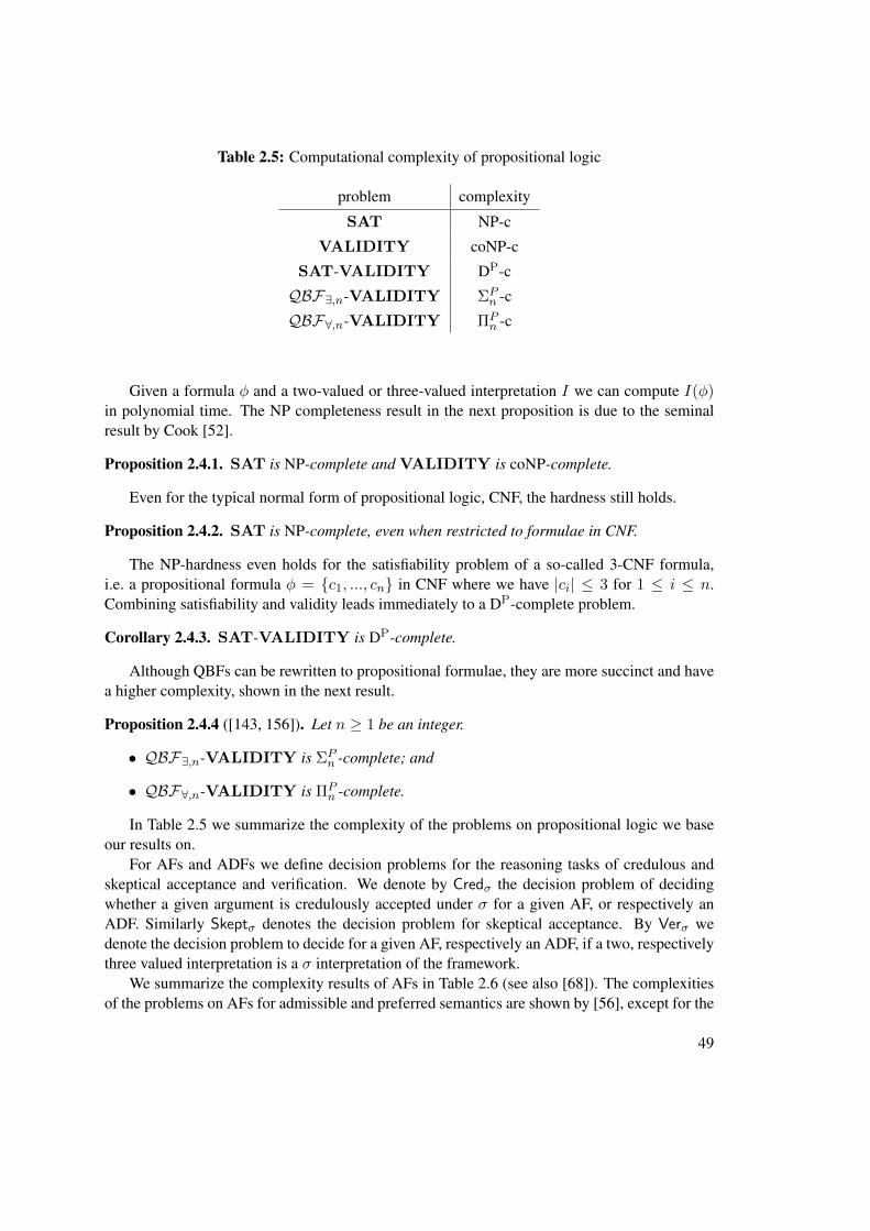
Table 2.5: Computational complexity of propositional logic

problem complexity

SAT NP-c

VALIDITY coNP-c

SAT-VALIDITY DP-c

QBF∃,n-VALIDITY ΣPn -c

QBF∀,n-VALIDITY ΠPn -c

Given a formula φ and a two-valued or three-valued interpretation I we can compute I(φ)in polynomial time. The NP completeness result in the next proposition is due to the seminalresult by Cook [52].

Proposition 2.4.1. SAT is NP-complete and VALIDITY is coNP-complete.

Even for the typical normal form of propositional logic, CNF, the hardness still holds.

Proposition 2.4.2. SAT is NP-complete, even when restricted to formulae in CNF.

The NP-hardness even holds for the satisfiability problem of a so-called 3-CNF formula,i.e. a propositional formula φ = {c1, ..., cn} in CNF where we have |ci| ≤ 3 for 1 ≤ i ≤ n.Combining satisfiability and validity leads immediately to a DP-complete problem.

Corollary 2.4.3. SAT-VALIDITY is DP-complete.

Although QBFs can be rewritten to propositional formulae, they are more succinct and havea higher complexity, shown in the next result.

Proposition 2.4.4 ([143, 156]). Let n ≥ 1 be an integer.

• QBF∃,n-VALIDITY is ΣPn -complete; and

• QBF∀,n-VALIDITY is ΠPn -complete.

In Table 2.5 we summarize the complexity of the problems on propositional logic we baseour results on.

For AFs and ADFs we define decision problems for the reasoning tasks of credulous andskeptical acceptance and verification. We denote by Credσ the decision problem of decidingwhether a given argument is credulously accepted under σ for a given AF, or respectively anADF. Similarly Skeptσ denotes the decision problem for skeptical acceptance. By Verσ wedenote the decision problem to decide for a given AF, respectively an ADF, if a two, respectivelythree valued interpretation is a σ interpretation of the framework.

We summarize the complexity results of AFs in Table 2.6 (see also [68]). The complexitiesof the problems on AFs for admissible and preferred semantics are shown by [56], except for the

49

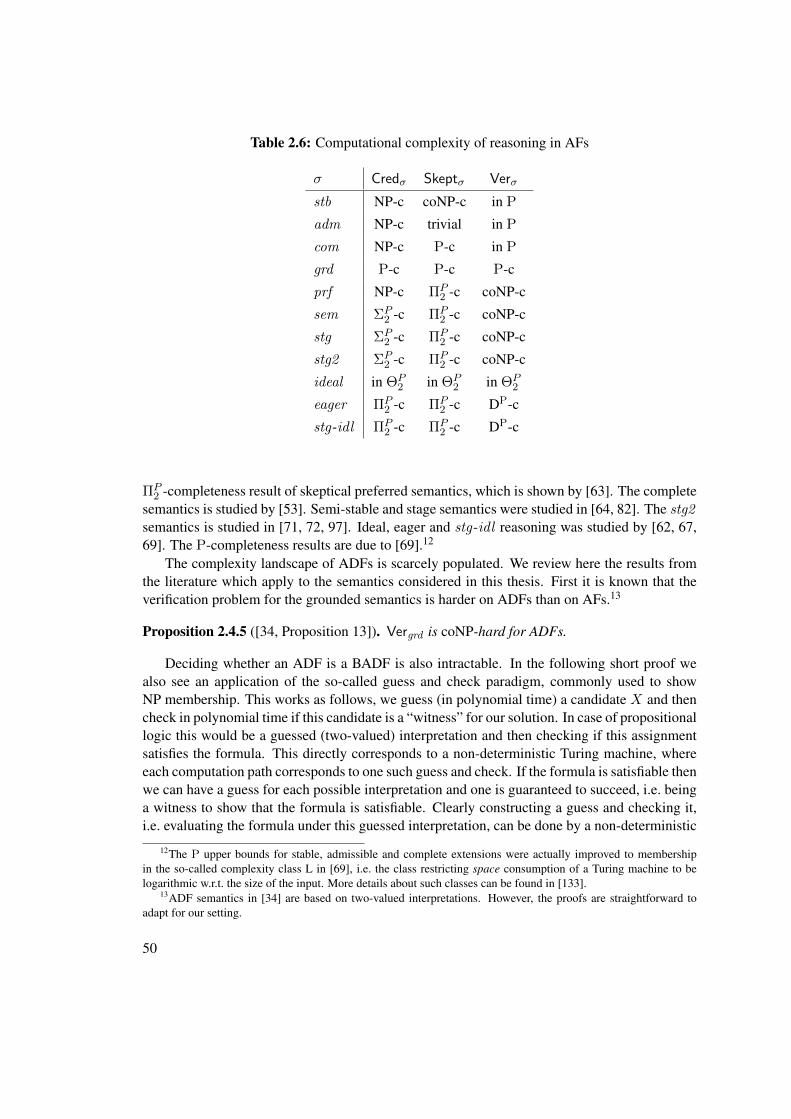
Table 2.6: Computational complexity of reasoning in AFs

σ Credσ Skeptσ Verσ

stb NP-c coNP-c in P

adm NP-c trivial in P

com NP-c P-c in P

grd P-c P-c P-c

prf NP-c ΠP2 -c coNP-c

sem ΣP2 -c ΠP

2 -c coNP-c

stg ΣP2 -c ΠP

2 -c coNP-c

stg2 ΣP2 -c ΠP

2 -c coNP-c

ideal in ΘP2 in ΘP

2 in ΘP2

eager ΠP2 -c ΠP

2 -c DP-c

stg-idl ΠP2 -c ΠP

2 -c DP-c

ΠP2 -completeness result of skeptical preferred semantics, which is shown by [63]. The complete

semantics is studied by [53]. Semi-stable and stage semantics were studied in [64, 82]. The stg2semantics is studied in [71, 72, 97]. Ideal, eager and stg-idl reasoning was studied by [62, 67,69]. The P-completeness results are due to [69].12

The complexity landscape of ADFs is scarcely populated. We review here the results fromthe literature which apply to the semantics considered in this thesis. First it is known that theverification problem for the grounded semantics is harder on ADFs than on AFs.13

Proposition 2.4.5 ([34, Proposition 13]). Vergrd is coNP-hard for ADFs.

Deciding whether an ADF is a BADF is also intractable. In the following short proof wealso see an application of the so-called guess and check paradigm, commonly used to showNP membership. This works as follows, we guess (in polynomial time) a candidate X and thencheck in polynomial time if this candidate is a “witness” for our solution. In case of propositionallogic this would be a guessed (two-valued) interpretation and then checking if this assignmentsatisfies the formula. This directly corresponds to a non-deterministic Turing machine, whereeach computation path corresponds to one such guess and check. If the formula is satisfiable thenwe can have a guess for each possible interpretation and one is guaranteed to succeed, i.e. beinga witness to show that the formula is satisfiable. Clearly constructing a guess and checking it,i.e. evaluating the formula under this guessed interpretation, can be done by a non-deterministic

12The P upper bounds for stable, admissible and complete extensions were actually improved to membershipin the so-called complexity class L in [69], i.e. the class restricting space consumption of a Turing machine to belogarithmic w.r.t. the size of the input. More details about such classes can be found in [133].

13ADF semantics in [34] are based on two-valued interpretations. However, the proofs are straightforward toadapt for our setting.

50

Turing machine in polynomial time. Furthermore we also see a typical coNP membership proofby considering the co-problem and showing NP membership.

Proposition 2.4.6 ([34, Proposition 14]). Deciding whether no link in a given ADF is dependentis coNP-complete.

Proof. Hardness was shown in [34, Proposition 14] (note that BADFs there allow redundantlinks). To see coNP membership consider the co-problem, i,e, deciding whether there exists adependent link in the ADF. Let D = (S,L,C) be an ADF and l ∈ L. We guess X,Y ⊆ S and(s, s′) = l ∈ L. We now check if l is dependent by verifying that X |= ϕs′ and X ∪ {s} 6|= ϕs′

for a counterexample that l is supporting. For the counterexample that l is attacking we verifythat Y 6|= ϕs′ and Y ∪ {s} |= ϕs′ . These checks can clearly be done in polynomial time.

Deciding the type of a link is in general also intractable.

Proposition 2.4.7. Deciding whether a given link in a given ADF is

1. attacking is coNP-complete;

2. supporting is coNP-complete;

3. dependent is NP-complete;

4. redundant is coNP-complete.

Proof. Item 1 was shown in [89, Proposition 4.4.1 and Proposition 4.4.2]. For showing item 2one can easily adapt the proof of [89, Proposition 4.4.1 and Proposition 4.4.2] for supportinglinks.

Let D = (S,L,C) be an ADF and l ∈ L. Showing that it is NP-complete to verify that l isdependent follows as a corollary from Proposition 2.4.6 (hardness follows from [34, Proposition14]). Lastly deciding if a link is redundant is the same as deciding if a link is attacking andsupporting, which can be done by two independent coNP-complete checks. Hence the problemis in coNP. For showing hardness consider the problem of deciding whether φ is a valid formula,which is a coNP-complete problem, see Proposition 2.4.1. We now reduce VALIDITY to thisproblem. Let φ be a formula, now define an ADF D = (S,L,C) with S = atoms(φ) ∪ {f}as follows. Let ϕx = x and ϕf = f ∨ φ. We assume w.l.o.g. that f /∈ atoms(φ). The ADFD can be constructed clearly in polynomial w.r.t. the size of φ. We now show that φ is valid iff(f, f) ∈ L is a redundant link. If φ is valid, then clearly there is no X ⊆ S s.t. X 6|= ϕf and(f, f) is attacking and supporting, thus redundant. Assume now that (f, f) is redundant. Thismeans that for any X ⊆ S we have X |= ϕf iff X ∪ {f} |= ϕf . Since {f} |= ϕf , we knowthat for any such X it holds that X |= ϕf . Thus for every Y ⊆ S with Y ∩ {f} = ∅ we haveY |= ϕf (since Y ∪ {f} |= ϕf ) and clearly Y ⊆ atoms(φ) and S \ {f} = atoms(φ) we knowthat any two-valued interpretation on φ must satisfy φ thus implying that φ is valid.

Finally a positive result is that the verification problem of the grounded semantics becomessignificantly easier on BADFs with known link types, i.e. it is tractable.

51

Proposition 2.4.8 ([34, Proposition 15]). Vergrd is in P for BADFs with known link types.

We greatly extend the complexity results for ADFs in Chapter 4. In particular we showthe computational complexity of the decision problems Credσ, Skeptσ and Verσ for ADFs andBADFs with known link types for semantics σ ∈ {adm, grd , prf }.

52

CHAPTER 3Advanced Algorithms for

Argumentation Frameworks

In this chapter we present novel algorithms for computationally hard problems defined on argu-mentation frameworks (AFs). In particular we develop algorithms for credulous and skepticalreasoning under preferred, semi-stable, stage, ideal, eager and stage-ideal semantics. Addition-ally our algorithms are capable of enumerating all extensions. Our algorithms rely on decisionprocedures for the Boolean satisfiability problem (SAT). The very basic idea is to delegate cer-tain computationally hard subtasks to a search engine capable of solving the SAT problem effi-ciently. A SAT-solver is a procedure, which receives as input a propositional formula and returnsa witness for satisfiability (a model) if the formula is satisfiable and “no” otherwise.

On the one hand delegating hard subtasks allows us to utilize existing efficient search enginesof modern SAT-solvers. This means we are able to re-use existing technology and researchdirectly. On the other hand we can, via an algorithm based on SAT-solvers, set up calls to thesolver iteratively using domain knowledge for the problem to solve. The overall workflow forour algorithms is shown in Figure 3.1. So first an AF, a semantics and a reasoning mode is givenas input. Then in the main procedure we construct Boolean queries for our SAT-solver. Afterpossibly multiple calls to the solver we arrive at our decision. In some cases we need a (simple)postprocessing step.

If one considers fully declarative approaches such as [85], which specify the whole problemin one encoding, and direct instantiations of algorithms for AF problems such as [131], then ourapproach can be seen as a hybrid variant of these two. In particular we have less declarative-ness by applying an imperative algorithm on top of more declarative queries and require someengineering effort to develop our algorithms. But we do not need to engineer search engines forcomputationally involving subtasks, e.g. NP-hard subtasks.

The algorithms developed for a semantics σ can be grouped into two categories. We callalgorithms of the first category search algorithms. The other category comprises of algorithmsrelying on advanced SAT technology, or SAT extensions. Intuitively, our search algorithms tra-verse a search space of a computationally easier semantics σ′, called base semantics, to compute

53

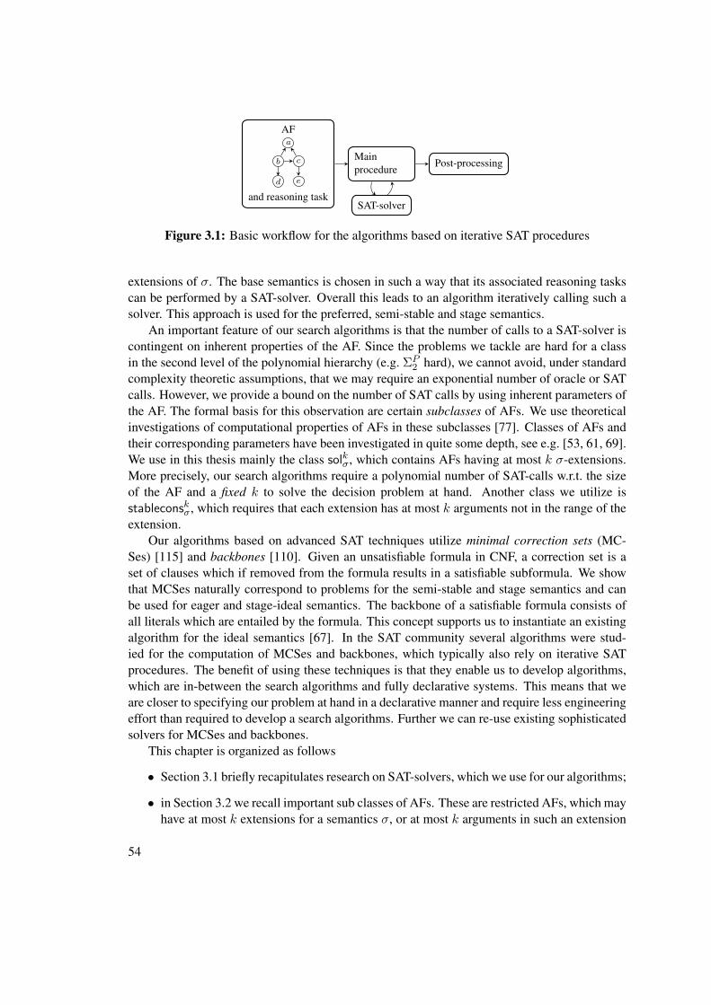
Mainprocedure

AF

d e

cb

a

and reasoning taskSAT-solver

Post-processing

Figure 3.1: Basic workflow for the algorithms based on iterative SAT procedures

extensions of σ. The base semantics is chosen in such a way that its associated reasoning taskscan be performed by a SAT-solver. Overall this leads to an algorithm iteratively calling such asolver. This approach is used for the preferred, semi-stable and stage semantics.

An important feature of our search algorithms is that the number of calls to a SAT-solver iscontingent on inherent properties of the AF. Since the problems we tackle are hard for a classin the second level of the polynomial hierarchy (e.g. ΣP

2 hard), we cannot avoid, under standardcomplexity theoretic assumptions, that we may require an exponential number of oracle or SATcalls. However, we provide a bound on the number of SAT calls by using inherent parameters ofthe AF. The formal basis for this observation are certain subclasses of AFs. We use theoreticalinvestigations of computational properties of AFs in these subclasses [77]. Classes of AFs andtheir corresponding parameters have been investigated in quite some depth, see e.g. [53, 61, 69].We use in this thesis mainly the class solkσ, which contains AFs having at most k σ-extensions.More precisely, our search algorithms require a polynomial number of SAT-calls w.r.t. the sizeof the AF and a fixed k to solve the decision problem at hand. Another class we utilize isstableconskσ, which requires that each extension has at most k arguments not in the range of theextension.

Our algorithms based on advanced SAT techniques utilize minimal correction sets (MC-Ses) [115] and backbones [110]. Given an unsatisfiable formula in CNF, a correction set is aset of clauses which if removed from the formula results in a satisfiable subformula. We showthat MCSes naturally correspond to problems for the semi-stable and stage semantics and canbe used for eager and stage-ideal semantics. The backbone of a satisfiable formula consists ofall literals which are entailed by the formula. This concept supports us to instantiate an existingalgorithm for the ideal semantics [67]. In the SAT community several algorithms were stud-ied for the computation of MCSes and backbones, which typically also rely on iterative SATprocedures. The benefit of using these techniques is that they enable us to develop algorithms,which are in-between the search algorithms and fully declarative systems. This means that weare closer to specifying our problem at hand in a declarative manner and require less engineeringeffort than required to develop a search algorithms. Further we can re-use existing sophisticatedsolvers for MCSes and backbones.

This chapter is organized as follows

• Section 3.1 briefly recapitulates research on SAT-solvers, which we use for our algorithms;

• in Section 3.2 we recall important sub classes of AFs. These are restricted AFs, which mayhave at most k extensions for a semantics σ, or at most k arguments in such an extension

54

which are not in the range of the extension;

• Section 3.3 develops search algorithms for the preferred, semi-stable and stage semantics.We first show a generic algorithm. Subsequently we instantiate this algorithm for theproblems at hand;

• lastly in Section 3.4 we apply existing algorithms for computing minimal correction setsand backbones of Boolean formulae to solve problems regarding the semi-stable, stage,eager, ideal and stage-ideal semantics.

Some of our results in this chapter are published. In [76, 77] we developed the searchalgorithms. The important complexity results underlying many of our approaches were derivedby Wolfgang Dvorák in [76]. The approaches using advanced SAT extensions were publishedin [153].

3.1 SAT Solving

In this section we briefly recall techniques for solving the SAT problem and introduce someuseful concepts for applications of SAT. Generally one considers as a satisfiability solver (SAT-solver) a search algorithm for finding a witness (a model) for satisfiability of a given formulaφ (in CNF), or proving unsatisfiability. Thereby these systems solve the famous NP-completeproblem of Boolean satisfiability. Even though this problem is in general intractable, contem-porary SAT-solvers such as MiniSAT [84] are capable of solving instances with hundreds ofthousands of literals and clauses.

Algorithms underlying such solvers have been under research for many years. The successof SAT-solvers is owed not only to successful theoretical research. In the so-called SAT compe-tition [108] solvers compete against each other and are evaluated w.r.t. their performance. Thecompetitions motivated efforts to come up with novel solving techniques.

Conflict-driven clause learning Modern SAT-solvers incorporate numerous techniques forfinding a model of a given formula. One of the most successful techniques is called conflict-driven clause learning (CDCL) [124, 123, 158]. We illustrate here the main ideas of this ap-proach. CDCL is a general concept and certain aspects may vary in concrete CDCL algorithms.First we introduce some basic terminology of SAT solving. Let φ be a Boolean formula. ManySAT-solvers construct a witness for φ’s satisfiability, or prove unsatisfiability, by iteratively as-signing variables to truth values in a partial interpretation I . There are two important kinds ofassignments. A SAT-solver may assign a value to a variable by a decision or by propagation.Assignments that are propagated are forced by the current partial assignment, whereas a SAT-solver chooses assignments for decisions usually through heuristics. Every time a SAT-solverdecides on a value a corresponding decision level l is incremented by one, which is initially 0(nothing is decided).

Assignment by propagation is computed by a fundamental concept called Boolean constraintpropagation (BCP). BCP refers to extending a current partial assignment I to I ′ by propagationon the formula φ. I ′ extends I if I = I ′|dom(I). Consider a partial assignment I with dom(I) =

55

{x1, . . . , xn−1} and a clause c = {l1, . . . , ln} ∈ φ with atoms(li) = {xi} for 1 ≤ i ≤ n. Thatis, I assigns to all literals in c a value, except for ln. Assume that I(li) = f for all 1 ≤ i ≤ n−1.Then the only possibility for an I ′, which extends I , to satisfy c is to evaluate ln to true. This canonly be achieved by setting the value of xn, s.t. I ′(ln) = t. This means the value of xn is implied(or forced) by the clause c and the partial interpretation I . A special case of this procedure isif |c| = 1, i.e. c is unit. A SAT algorithm typically distinguishes between assignments madeby a decision and assignments forced by BCP. Like decisions, propagated assignments have acorresponding decision level, namely the level at which BCP inferred the assignment. A CDCLmay backtrack to a certain decision level l. Then all decisions and propagations at levels l′ > lare erased (or reverted).

The idea of CDCL is now to decide upon values for variables, applying BCP on the currentpartial interpretation and in case of a conflict c, backtracking and augmenting the given formulaφ with so-called learnt clauses. Learnt clauses are crucial for correctness and performance ofa CDCL algorithm. Using learnt clauses one avoids to re-visit parts of the search space. ACDCL algorithm starts with decision level l = 0 and the initial partial interpretation assigningno variables. At each decision level BCP is applied to propagate values of the current partialinterpretation. If no conflict is revealed through BCP, i.e. no clause is unsatisfied by the currentpartial interpretation, then a CDCL algorithm decides the value for the next unassigned variable.If BCP revealed a conflict via clause c ∈ φ, i.e. I 6|= c, then the algorithm learns a clause c′

by conjoining it with φ and backtracks to a lower decision level. The clause c′ is constructedby inspecting the so-called implication graph. From this graph a CDCL algorithm infers thedecisions which lead to the conflict c. The implication graph is a directed graph, whose verticesconsist of assigned and propagated literals and the clause c. There is a directed edge (l1, l2)in this graph if l2 was propagated by BCP using l1. Additionally all literals with variables inatoms(c) have a directed edge to c. This means that all assignments by decisions have noincoming edges. The decisions which lead to the conflict c are those vertices correspondingto decisions without incoming edges that have a path to c. There are different strategies forlearning a clause from the implication graph. One possibility is to construct the negation of theconjunction of literals which lead to the conflict c, which is equivalent to a clause c′. CDCLalgorithms make sure that φ |= c′ holds.

If a clause c′ is learnt the algorithm backtracks. Here again CDCL algorithms differ in termsof their backtracking strategy. One choice is to backtrack to the highest decision level of thecorresponding decision variables in c′, excluding the decision variable of the current decisionlevel. For example assume that the current decision level is l = 2 and we have the decisionsp@1 and q@2, denoting that we decided to assign p to true at level one and q to true at level 2.Further assume that we learnt the clause c′ = (¬p ∨ ¬q). Then we would backtrack to l = 1,since c′ contains two decision variables. If we exclude the most recent decision of q, then thehighest remaining decision is that of p at level 1. At the now lowered decision level BCP willpropagate the value of the most recent decision, before backtracking, to the opposite value asbefore. In the example, after backtracking we still have the partial assignment of p set to true.Thus BCP infers through c′ that q must be false. In this way the CDCL algorithm implicitly“flips” the value of the last decision by applying BCP on the learnt clause.

We show an example computation in Table 3.1. The initial formula is φ0. We assume a

56

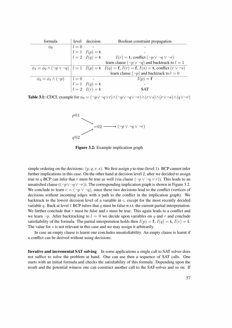
formula level decision Boolean constraint propagationφ0 l = 0 - -

l = 1 I(p) = t -l = 2 I(q) = t I(r) = t, conflict (¬p ∨ ¬q ∨ ¬r)

learn clause (¬p ∨ ¬q) and backtrack to l = 1

φ1 = φ0 ∧ (¬p ∨ ¬q) l = 1 I(p) = t I(q) = f , I(r) = f , I(s) = t, conflict (r ∨ ¬s)learn clause (¬p) and backtrack to l = 0

φ2 = φ1 ∧ (¬p) l = 0 - I(p) = fl = 1 I(q) = t -l = 2 I(r) = t SAT

Table 3.1: CDCL example for φ0 = (¬p∨¬q∨r)∧(¬p∨¬q∨¬r)∧(r∨s)∧(r∨¬s)∧(q∨¬r)

p@1

q@2

r@2 (¬p ∨ ¬q ∨ ¬r)

Figure 3.2: Example implication graph

simple ordering on the decisions: (p, q, r, s). We first assign p to true (level 1). BCP cannot inferfurther implications in this case. On the other hand at decision level 2, after we decided to assigntrue to q BCP can infer that r must be true as well (via clause (¬p ∨ ¬q ∨ r)). This leads to anunsatisfied clause ((¬p∨¬q∨¬r)). The corresponding implication graph is shown in Figure 3.2.We conclude to learn c = (¬p ∨ ¬q), since these two decisions lead to the conflict (vertices ofdecisions without incoming edges with a path to the conflict in the implication graph). Webacktrack to the lowest decision level of a variable in c, except for the most recently decidedvariable q. Back at level 1 BCP infers that q must be false w.r.t. the current partial interpretation.We further conclude that r must be false and s must be true. This again leads to a conflict andwe learn ¬p. After backtracking to l = 0 we decide upon variables on q and r and concludesatisfiability of the formula. The partial interpretation holds then I(p) = f , I(q) = t, I(r) = t.The value for s is not relevant in this case and we may assign it arbitrarily.

In case an empty clause is learnt one concludes unsatisfiability. An empty clause is learnt ifa conflict can be derived without using decisions.

Iterative and incremental SAT solving In some applications a single call to SAT solver doesnot suffice to solve the problem at hand. One can use then a sequence of SAT calls. Onestarts with an initial formula and checks the satisfiability of this formula. Depending upon theresult and the potential witness one can construct another call to the SAT-solver and so on. If

57

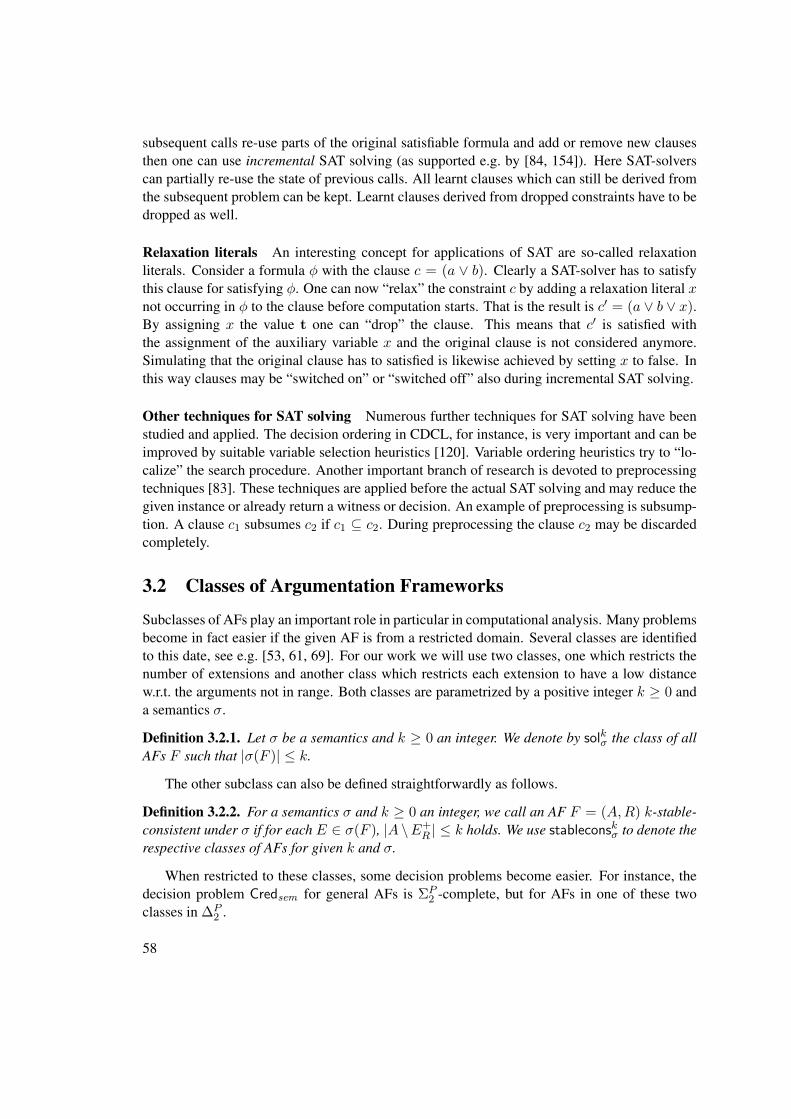
subsequent calls re-use parts of the original satisfiable formula and add or remove new clausesthen one can use incremental SAT solving (as supported e.g. by [84, 154]). Here SAT-solverscan partially re-use the state of previous calls. All learnt clauses which can still be derived fromthe subsequent problem can be kept. Learnt clauses derived from dropped constraints have to bedropped as well.

Relaxation literals An interesting concept for applications of SAT are so-called relaxationliterals. Consider a formula φ with the clause c = (a ∨ b). Clearly a SAT-solver has to satisfythis clause for satisfying φ. One can now “relax” the constraint c by adding a relaxation literal xnot occurring in φ to the clause before computation starts. That is the result is c′ = (a ∨ b ∨ x).By assigning x the value t one can “drop” the clause. This means that c′ is satisfied withthe assignment of the auxiliary variable x and the original clause is not considered anymore.Simulating that the original clause has to satisfied is likewise achieved by setting x to false. Inthis way clauses may be “switched on” or “switched off” also during incremental SAT solving.

Other techniques for SAT solving Numerous further techniques for SAT solving have beenstudied and applied. The decision ordering in CDCL, for instance, is very important and can beimproved by suitable variable selection heuristics [120]. Variable ordering heuristics try to “lo-calize” the search procedure. Another important branch of research is devoted to preprocessingtechniques [83]. These techniques are applied before the actual SAT solving and may reduce thegiven instance or already return a witness or decision. An example of preprocessing is subsump-tion. A clause c1 subsumes c2 if c1 ⊆ c2. During preprocessing the clause c2 may be discardedcompletely.

3.2 Classes of Argumentation Frameworks

Subclasses of AFs play an important role in particular in computational analysis. Many problemsbecome in fact easier if the given AF is from a restricted domain. Several classes are identifiedto this date, see e.g. [53, 61, 69]. For our work we will use two classes, one which restricts thenumber of extensions and another class which restricts each extension to have a low distancew.r.t. the arguments not in range. Both classes are parametrized by a positive integer k ≥ 0 anda semantics σ.

Definition 3.2.1. Let σ be a semantics and k ≥ 0 an integer. We denote by solkσ the class of allAFs F such that |σ(F )| ≤ k.

The other subclass can also be defined straightforwardly as follows.

Definition 3.2.2. For a semantics σ and k ≥ 0 an integer, we call an AF F = (A,R) k-stable-consistent under σ if for each E ∈ σ(F ), |A \E+

R | ≤ k holds. We use stableconskσ to denote therespective classes of AFs for given k and σ.

When restricted to these classes, some decision problems become easier. For instance, thedecision problem Credsem for general AFs is ΣP

2 -complete, but for AFs in one of these twoclasses in ∆P

2 .

58

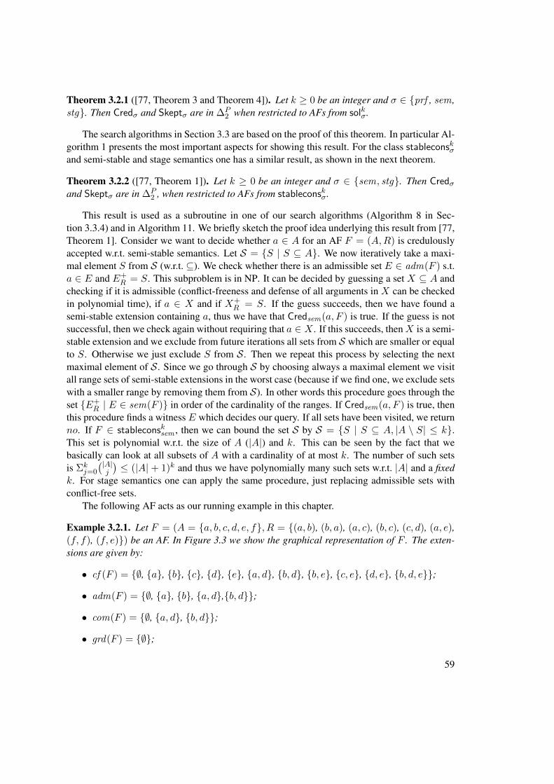
Theorem 3.2.1 ([77, Theorem 3 and Theorem 4]). Let k ≥ 0 be an integer and σ ∈ {prf , sem ,stg}. Then Credσ and Skeptσ are in ∆P

2 when restricted to AFs from solkσ.

The search algorithms in Section 3.3 are based on the proof of this theorem. In particular Al-gorithm 1 presents the most important aspects for showing this result. For the class stableconskσand semi-stable and stage semantics one has a similar result, as shown in the next theorem.

Theorem 3.2.2 ([77, Theorem 1]). Let k ≥ 0 be an integer and σ ∈ {sem, stg}. Then Credσand Skeptσ are in ∆P

2 , when restricted to AFs from stableconskσ.

This result is used as a subroutine in one of our search algorithms (Algorithm 8 in Sec-tion 3.3.4) and in Algorithm 11. We briefly sketch the proof idea underlying this result from [77,Theorem 1]. Consider we want to decide whether a ∈ A for an AF F = (A,R) is credulouslyaccepted w.r.t. semi-stable semantics. Let S = {S | S ⊆ A}. We now iteratively take a maxi-mal element S from S (w.r.t. ⊆). We check whether there is an admissible set E ∈ adm(F ) s.t.a ∈ E and E+

R = S. This subproblem is in NP. It can be decided by guessing a set X ⊆ A andchecking if it is admissible (conflict-freeness and defense of all arguments in X can be checkedin polynomial time), if a ∈ X and if X+

R = S. If the guess succeeds, then we have found asemi-stable extension containing a, thus we have that Credsem(a, F ) is true. If the guess is notsuccessful, then we check again without requiring that a ∈ X . If this succeeds, thenX is a semi-stable extension and we exclude from future iterations all sets from S which are smaller or equalto S. Otherwise we just exclude S from S. Then we repeat this process by selecting the nextmaximal element of S . Since we go through S by choosing always a maximal element we visitall range sets of semi-stable extensions in the worst case (because if we find one, we exclude setswith a smaller range by removing them from S). In other words this procedure goes through theset {E+

R | E ∈ sem(F )} in order of the cardinality of the ranges. If Credsem(a, F ) is true, thenthis procedure finds a witness E which decides our query. If all sets have been visited, we returnno. If F ∈ stableconsksem , then we can bound the set S by S = {S | S ⊆ A, |A \ S| ≤ k}.This set is polynomial w.r.t. the size of A (|A|) and k. This can be seen by the fact that webasically can look at all subsets of A with a cardinality of at most k. The number of such setsis Σk

j=0

(|A|j

)≤ (|A| + 1)k and thus we have polynomially many such sets w.r.t. |A| and a fixed

k. For stage semantics one can apply the same procedure, just replacing admissible sets withconflict-free sets.

The following AF acts as our running example in this chapter.

Example 3.2.1. Let F = (A = {a, b, c, d, e, f}, R = {(a, b), (b, a), (a, c), (b, c), (c, d), (a, e),(f, f), (f, e)}) be an AF. In Figure 3.3 we show the graphical representation of F . The exten-sions are given by:

• cf (F ) = {∅, {a}, {b}, {c}, {d}, {e}, {a, d}, {b, d}, {b, e}, {c, e}, {d, e}, {b, d, e}};

• adm(F ) = {∅, {a}, {b}, {a, d},{b, d}};

• com(F ) = {∅, {a, d}, {b, d}};

• grd(F ) = {∅};

59

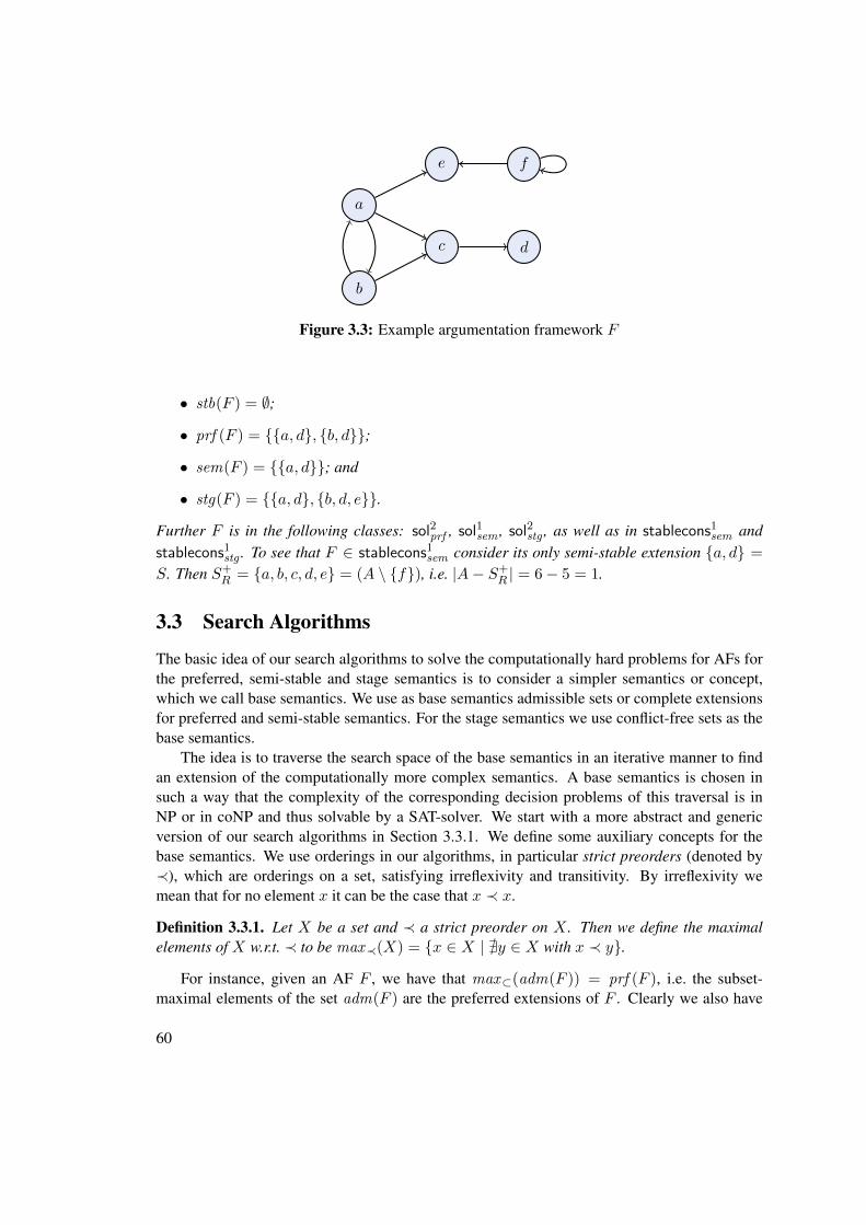
a

b

c d

e f

Figure 3.3: Example argumentation framework F

• stb(F ) = ∅;

• prf (F ) = {{a, d}, {b, d}};

• sem(F ) = {{a, d}}; and

• stg(F ) = {{a, d}, {b, d, e}}.

Further F is in the following classes: sol2prf , sol1sem , sol2stg , as well as in stablecons1sem andstablecons1stg . To see that F ∈ stablecons1sem consider its only semi-stable extension {a, d} =

S. Then S+R = {a, b, c, d, e} = (A \ {f}), i.e. |A− S+

R | = 6− 5 = 1.

3.3 Search Algorithms

The basic idea of our search algorithms to solve the computationally hard problems for AFs forthe preferred, semi-stable and stage semantics is to consider a simpler semantics or concept,which we call base semantics. We use as base semantics admissible sets or complete extensionsfor preferred and semi-stable semantics. For the stage semantics we use conflict-free sets as thebase semantics.

The idea is to traverse the search space of the base semantics in an iterative manner to findan extension of the computationally more complex semantics. A base semantics is chosen insuch a way that the complexity of the corresponding decision problems of this traversal is inNP or in coNP and thus solvable by a SAT-solver. We start with a more abstract and genericversion of our search algorithms in Section 3.3.1. We define some auxiliary concepts for thebase semantics. We use orderings in our algorithms, in particular strict preorders (denoted by≺), which are orderings on a set, satisfying irreflexivity and transitivity. By irreflexivity wemean that for no element x it can be the case that x ≺ x.

Definition 3.3.1. Let X be a set and ≺ a strict preorder on X . Then we define the maximalelements of X w.r.t. ≺ to be max≺(X) = {x ∈ X | @y ∈ X with x ≺ y}.

For instance, given an AF F , we have that max⊂(adm(F )) = prf (F ), i.e. the subset-maximal elements of the set adm(F ) are the preferred extensions of F . Clearly we also have

60

max⊂(com(F )) = prf (F ). For the semi-stable and stage semantics one can use the followingorder which uses the range of arguments in an AF.

Definition 3.3.2. Let F = (A,R) be an AF and S, T ⊆ A. We define the ordering ≺R on 2A tobe S ≺R T iff S+

R ⊂ T+R .

It is easy to show that ≺R is indeed a strict preorder.

Proposition 3.3.1. Let F = (A,R) be an AF. Then ≺R is a strict preorder.

Proof. Let S, T, U ⊆ A. Since S+R 6⊂ S+

R we have that ≺R is irreflexive. Assume that S ≺R Tand T ≺R U . Then we have S+

R ⊂ T+R and T+

R ⊂ U+R . Since ⊂ is transitive we have S+

R ⊂ U+R

and thus S ≺R U , implying that ≺R is transitive.

As expected, we have for any AF F that the following equations hold.

Proposition 3.3.2. Let F = (A,R) be an AF. It holds that

• max⊂(adm(F )) = max⊂(com(F )) = prf (F );

• max≺R(adm(F )) = max≺R(com(F )) = max≺R(prf (F )) = sem(F ); and

• max≺R(cf (F )) = stg(F ).

Proof. Only the equation max≺R(prf (F )) = sem(F ) does not follow directly from definition.We know that prf (F ) ⊆ sem(F ). Assume E ∈ max≺R(prf (F )). Suppose there is an E′ ∈sem(F ), s.t. E ≺R E′ (which would imply E /∈ sem(F )). Then E′ ∈ prf (F ) and E′ ∈max≺R(prf (F )). This is a contradiction to E being ≺R-maximal.

Assume E ∈ sem(F ). Then E ∈ prf (F ). There is no E′ ∈ adm(F ), s.t. E ≺R E′.Therefore such an E′ is also not present in prf (F ). Therefore E ∈ max≺R(prf (F )).

3.3.1 Generic Algorithm

In this section we present a generic version of our search algorithms. The generic algorithmmakes two types of function calls, which can be implemented with a SAT-solver. These twofunction calls can be represented by checking if a certain set is empty, and if not computingone member of it. This naturally corresponds to a SAT call, which checks whether a formula issatisfiable and if yes, returns a model. The two sets are defined as follows

Definition 3.3.3. Let F = (A,R) be an AF, σ a semantics on AFs, S ⊆ σ(F ), X ∈ σ(F ) and≺ a strict preorder on 2A. Define the following two subsets of σ-extensions

• ExtsExcl(σ, F,S,≺) = {E ∈ σ(F ) | @E′ ∈ S s.t. E ≺ E′ or E = E′};

• GreaterExts(σ, F,X,≺) = {E ∈ σ(F ) | X ≺ E}.

61

The intended meaning of these sets is that both contain candidates to a desired solutionor extension. The set ExtsExcl(σ, F,S,≺) contains a subset of all the extensions of F w.r.t.semantics σ, i.e. ExtsExcl(σ, F,S,≺) ⊆ σ(F ), s.t. no extension in this set is smaller to one inS w.r.t. the order ≺ or is identical with one in S. Thereby we can exclude previously computedextensions. Since our task is always to compute extensions of semantics satisfying some formof maximality, we can also exclude all candidates smaller to the ones in S . One can view the setS as the extensions already computed (or visited).

On the other hand GreaterExts(σ, F,X,≺) contains all σ extensions of F which are greaterthanX w.r.t.≺. Simply put, this allows us to iteratively find a greater candidate w.r.t. an orderingto reach a desired extension.

The next rather technical lemma shows a basic property of these two sets, which will beuseful for showing termination of the following algorithms.

Lemma 3.3.3. Let F = (A,R) be an AF, σ a semantics on AFs and ≺ a strict preorder on 2A.Further let (i) S,S ′ ⊆ σ(F ) with S ⊂ S ′ s.t. there exists a D′ ∈ (S ′ \ S) with D′ 6≺ D for allD ∈ S and (ii) X,X ′ ∈ σ(F ) with X ≺ X ′. It holds that

• ExtsExcl(σ, F,S,≺) ⊃ ExtsExcl(σ, F,S ′,≺); and

• GreaterExts(σ, F,X,≺) ⊃ GreaterExts(σ, F,X ′,≺).

Proof. Let ExtsExcl(σ, F,S,≺) = E and ExtsExcl(σ, F,S ′,≺) = E ′. We now need to showthat E ⊃ E ′. Clearly we have E , E ′ ⊆ σ(F ). If E′ ∈ E ′, then E′ ∈ σ(F ) and there is no S′ ∈ S ′s.t. E′ ≺ S′ and E′ /∈ S ′. Therefore E′ ∈ E , since S ⊂ S ′ and thus there is also no S ∈ S s.t.E′ ≺ S. Now consider an element D′ ∈ (S ′ \ S) with D′ 6≺ D for all D ∈ S, which exists dueto the assumptions in the lemma. Clearly D′ /∈ E ′. Since there is also no D ∈ S s.t. D′ ≺ Dand also D′ /∈ S, this means that D′ ∈ E . Thus E ⊃ E ′.

Now let GreaterExts(σ, F,X,≺) = G and GreaterExts(σ, F,X ′,≺) = G′. Let E′ ∈ G′.This means that X ≺ X ′ ≺ E′ (recall that ≺ is transitive). Thus clearly E′ ∈ G. Now it isstraightforward to see that X ′ /∈ G′, since X ′ 6≺ X ′. But since X ≺ X ′ this means that X ′ ∈ G.Thus G ⊃ G′.

This leads to our generic Algorithm 1 for computing credulous or skeptical acceptance of anargument a in an AF w.r.t. a semantics σ or enumerating all extensions from σ(F ).

Algorithm 1 is parametrized by an AF F , an argument a to query under mode M and asemantics σ. The two further parameters σ′ and ≺ enable us to actually compute this resultusing the base semantics σ′ to search for its maximal elements w.r.t. ≺. In Figure 3.4 we seean example computation of this algorithm. The ellipse represents the extensions of the basesemantics σ′. In the first step (top in the figure) we find an arbitrary member of it, say E0

0 ,for the first outer while loop (lines 2–10) and inner while loop (lines 3–5). Then we iterativelygenerate new candidates in the inner while loop, which are greater w.r.t. ≺. This is representedon the right side of the figure. At some point we reach a maximal element E0

n. This is oneextension in σ(F ). In the next iteration of the outer while loop, in the middle of the figure,we exclude E0

n and all E ≺ E0n from the search space (gray area) and repeat the process as

before. Finally at the bottom of the figure we reach the final state, where we have identified all

62

Algorithm 1 Generic(F, a,M, σ, σ′,≺)

Require: AF F = (A,R), argument a ∈ A, mode M ∈ {Enum,Cred, co-Skept}, semanticsσ and σ′, ≺ a strict preorder on 2A and σ(F ) = max≺(σ′(F ))

Ensure: returns S = σ(F ) if M = Enum, yes if M = Cred (co-Skept) and Credσ(a, F ) =yes (Skeptσ(a, F ) = no), otherwise no

1: S := ∅2: while ∃E,E ∈ ExtsExcl(σ′, F,S,≺) do3: while ∃E′, E′ ∈ GreaterExts(σ′, F, E,≺) do4: E := E′

5: end while6: if M = Cred and a ∈ E or M = co-Skept and a /∈ E then7: return yes8: end if9: S := S ∪ {E}

10: end while11: return no (or S if M = Enum)

σ′(F )

E00

E0n

E00 ≺ E0

1 ≺ · · · ≺ E0n

E0n

E10

E1n′

E10 ≺ E1

1 ≺ · · · ≺E1n′

...σ(F )

E0nE1

n′Emn′′

Figure 3.4: Illustration of Algorithm 1

63

members of σ(F ) = {E0n, E

1n′ , . . . , E

mn′′}. The correctness of this generic algorithm is shown

next. Note for showing the termination of the algorithm, i.e. that it finishes computation after afinite number of steps, we apply our general assumption that AFs are finite.

Theorem 3.3.4. Let F = (A,R) be an AF, a ∈ A, M ∈ {Cred, co-Skept,Enum}, σ and σ′ AFsemantics, ≺ a strict preorder on 2A and σ(F ) = max≺(σ′(F )). Then

• Generic(F, a,M, σ, σ′,≺) terminates;

• Credσ(a, F ) = yes iff Generic(F, a,Cred, σ, σ′,≺) returns yes;

• Skeptσ(a, F ) = yes iff Generic(F, a, co-Skept, σ, σ′,≺) returns no;

• Generic(F, a,Enum, σ, σ′,≺) returns σ(F ) = S.

Proof. We first show that Generic(F, a,M, σ, σ′,≺) terminates. We assume that |A| ≥ 0 and|R| ≥ 0 are finite integers in our proof. W.l.o.g. we assume that M = Enum, since for the othermodes the algorithm just might terminate earlier, i.e. returning “yes”. It is straightforward to seethat both ExtsExcl(σ′, F,S,≺) and GreaterExts(σ′, F, E,≺) are finite, since σ′(F ) is finite.We first show that for any σ′, F , E ∈ σ(F ) and ≺ as defined in the assumptions that the “inner”while-loop in lines 3–5 terminates. This follows from Lemma 3.3.3, which shows that both setsdecrease with each iteration in the corresponding while loop. To see that the assumptions ofLemma 3.3.3 are fulfilled consider for the inner while loop that if GreaterExts(σ′, F, E,≺) isnon-empty then an E′ out of it is selected. We clearly have that E ≺ E′. For the outer whileloop if ExtsExcl(σ′, F,S,≺) is non-empty, then we choose an E out of it s.t. E 6≺ D for anyD ∈ S. Clearly this also holds for the E added in Line 9 to S. Therefore in the next iteration wehave that S is a superset of the set in the previous iteration and contains one member, which isnot smaller w.r.t. ≺ or equal than all its members from the previous iteration. This implies thatboth loops terminate since both sets start in each loop with a finite cardinality, which decreasesby at least one in each step and the loops terminate if the corresponding sets are empty.

We prove now the last claim, since the decision problems follow straightforwardly. Assumeagain M = Enum. We now have to show that Generic(F, a,Enum, σ, σ′,≺) returns σ(F ) =S = max≺(σ′(F )). There are three cases to consider.

• The trivial case occurs if σ′(F ) = ∅. Then σ(F ) is also empty and the outer while loopterminates immediately and we return S = ∅.

• Assume the algorithm terminated and X ∈ S with σ′(F ) 6= ∅. We now show that thenalso X ∈ σ(F ). Clearly if σ′(F ) is non-empty so is ExtsExcl(σ′, F, ∅,≺). Then we canconclude thatX ∈ σ′(F ), since it must be either in GreaterExts(σ′, F, E,≺) for some Eor in ExtsExcl(σ′, F,S ′,≺) for some S ′. Suppose there exists an X ′ ∈ σ′(F ) such thatX ≺ X ′. This is a counterexample that X ∈ σ(F ). Then the inner while loop did notterminate, since we have that GreaterExts(σ′, F,X,≺) is not empty. Thus it follows thatX ∈ σ(F ).

64

• Now assume the algorithm terminated and returned S and X ∈ σ(F ). We show that Xis also in S. It is easy to see that X ∈ ExtsExcl(σ′, F, ∅,≺). Suppose that X /∈ S.But then ExtsExcl(σ′, F,S,≺) cannot be empty, since there is no element X ′ ∈ σ′(F )s.t. X ≺ X ′. Thus there does not exist a D ∈ S s.t. X ≺ D and we can derive thatX ∈ ExtsExcl(σ′, F,S,≺). Therefore the algorithm cannot have terminated.

Since σ(F ) = S if M = Enum, it follows that for any E ∈ σ(F ) we enter the outer whileloop once. If this E solves the question of credulous acceptance of an argument a positively,then we exit in Line 7 if M = Cred. The case for co-skeptical acceptance is analogous. In allthe other cases we return “no” as specified.

Considering that all computations in Algorithm 1 are easy to compute, except for the twomembership checks in Line 2 and Line 3, it is useful to calculate how many of these checks arerequired in the worst case. We view these two lines as function calls and next show the relationof the given AF and the number of required function calls. Note that we assume here a concretestrict preorder for our extensions: either ⊂ or ≺R. The reason for this choice is that arbitrarypreorders may have exponentially many improvement steps.

Proposition 3.3.5. Let F = (A,R) be an AF, a ∈ A, σ and σ′ AF semantics, ≺∈ {⊂,≺R}and σ(F ) = max≺(σ′(F )). The number of function calls (Line 2 and Line 3 of Algorithm 1) ofGeneric(F, a,M, σ, σ′,≺) for M ∈ {Cred, co-Skept,Enum} is O(|A| · |σ(F )|).

Proof. The proposition follows from the proof of Theorem 3.3.4. Simply consider that the outerwhile loop is entered at most |σ(F )| times and the inner while loop must terminate after at most|A| iterations, since if E ⊂ E′, then |E| < |E′| and if E ≺R E′, then |E+

R | < |E′+R | and in bothcases at most |A| arguments can be added to the set or the range of a set.

The upper bound for the running time w.r.t. the function calls also holds for concrete in-stantiations of Algorithm 1 for preferred semantics in Section 3.3.2 and semi-stable and stagesemantics in Section 3.3.3. Thus if F ∈ solkσ, for a fixed integer k, then we have a ∆P

2 procedurefor solving credulous or skeptical reasoning under semantics σ, since |A| · k is polynomial w.r.t.the size of the AF and k.

3.3.2 Search Algorithms for Preferred Semantics

We now instantiate the generic Algorithm 1 for preferred semantics. By looking at Proposi-tion 3.3.2 we can infer two base semantics for preferred semantics, admissible sets and completeextensions. For the relation we simply require a subset relation between extensions. This leadsto Algorithm 2. We now show how this algorithm fares on our running Example 3.2.1.

Example 3.3.1. Consider the AF from Example 3.2.1. We show the execution of Algorithm 2 foradmissible sets as the base semantics. After initializing S to the empty set we come to Line 2(the outer while loop) for the first time. Then ExtsExcl(adm, F, ∅,⊂) = adm(F ) = {∅, {a},{b}, {a, d}, {b, d}}. The algorithm itself is defined in a non-deterministic way, i.e. it may returnany member of this set. Assume that E = ∅ was selected. Then GreaterExts(adm, F, E,⊂) =adm(F )\{∅}. In a subsequent step we might choose {a} and afterwards {a, d}. This set cannot

65

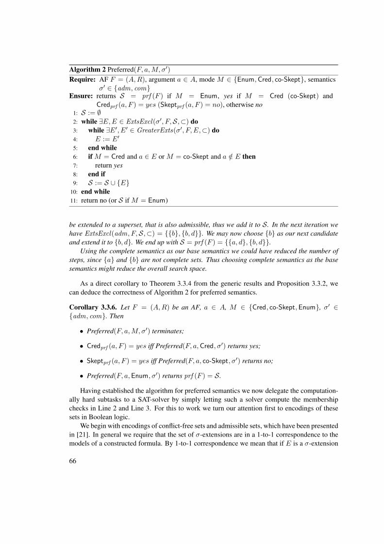
Algorithm 2 Preferred(F, a,M, σ′)

Require: AF F = (A,R), argument a ∈ A, mode M ∈ {Enum,Cred, co-Skept}, semanticsσ′ ∈ {adm, com}

Ensure: returns S = prf (F ) if M = Enum, yes if M = Cred (co-Skept) andCredprf (a, F ) = yes (Skeptprf (a, F ) = no), otherwise no

1: S := ∅2: while ∃E,E ∈ ExtsExcl(σ′, F,S,⊂) do3: while ∃E′, E′ ∈ GreaterExts(σ′, F, E,⊂) do4: E := E′



be extended to a superset, that is also admissible, thus we add it to S. In the next iteration wehave ExtsExcl(adm, F,S,⊂) = {{b}, {b, d}}. We may now choose {b} as our next candidateand extend it to {b, d}. We end up with S = prf (F ) = {{a, d}, {b, d}}.

Using the complete semantics as our base semantics we could have reduced the number ofsteps, since {a} and {b} are not complete sets. Thus choosing complete semantics as the basesemantics might reduce the overall search space.

As a direct corollary to Theorem 3.3.4 from the generic results and Proposition 3.3.2, wecan deduce the correctness of Algorithm 2 for preferred semantics.

Corollary 3.3.6. Let F = (A,R) be an AF, a ∈ A, M ∈ {Cred, co-Skept,Enum}, σ′ ∈{adm, com}. Then

• Preferred(F, a,M, σ′) terminates;

• Credprf (a, F ) = yes iff Preferred(F, a,Cred, σ′) returns yes;

• Skeptprf (a, F ) = yes iff Preferred(F, a, co-Skept, σ′) returns no;

• Preferred(F, a,Enum, σ′) returns prf (F ) = S .

Having established the algorithm for preferred semantics we now delegate the computation-ally hard subtasks to a SAT-solver by simply letting such a solver compute the membershipchecks in Line 2 and Line 3. For this to work we turn our attention first to encodings of thesesets in Boolean logic.

We begin with encodings of conflict-free sets and admissible sets, which have been presentedin [21]. In general we require that the set of σ-extensions are in a 1-to-1 correspondence to themodels of a constructed formula. By 1-to-1 correspondence we mean that if E is a σ-extension

66

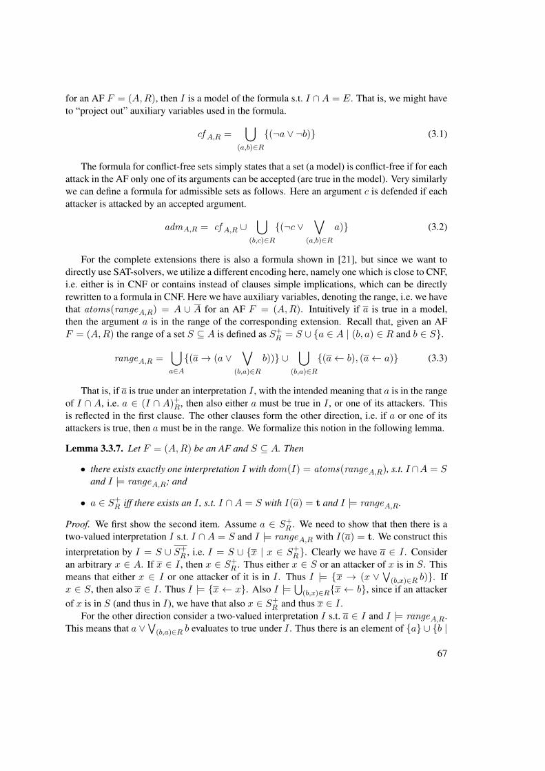
for an AF F = (A,R), then I is a model of the formula s.t. I ∩A = E. That is, we might haveto “project out” auxiliary variables used in the formula.

cf A,R =⋃

(a,b)∈R

{(¬a ∨ ¬b)} (3.1)

The formula for conflict-free sets simply states that a set (a model) is conflict-free if for eachattack in the AF only one of its arguments can be accepted (are true in the model). Very similarlywe can define a formula for admissible sets as follows. Here an argument c is defended if eachattacker is attacked by an accepted argument.

admA,R = cf A,R ∪⋃

(b,c)∈R

{(¬c ∨∨

(a,b)∈R

a)} (3.2)

For the complete extensions there is also a formula shown in [21], but since we want todirectly use SAT-solvers, we utilize a different encoding here, namely one which is close to CNF,i.e. either is in CNF or contains instead of clauses simple implications, which can be directlyrewritten to a formula in CNF. Here we have auxiliary variables, denoting the range, i.e. we havethat atoms(rangeA,R) = A ∪ A for an AF F = (A,R). Intuitively if a is true in a model,then the argument a is in the range of the corresponding extension. Recall that, given an AFF = (A,R) the range of a set S ⊆ A is defined as S+

R = S ∪ {a ∈ A | (b, a) ∈ R and b ∈ S}.

rangeA,R =⋃a∈A{(a→ (a ∨

∨(b,a)∈R

b))} ∪⋃

(b,a)∈R

{(a← b), (a← a)} (3.3)

That is, if a is true under an interpretation I , with the intended meaning that a is in the rangeof I ∩ A, i.e. a ∈ (I ∩ A)+

R, then also either a must be true in I , or one of its attackers. Thisis reflected in the first clause. The other clauses form the other direction, i.e. if a or one of itsattackers is true, then a must be in the range. We formalize this notion in the following lemma.

Lemma 3.3.7. Let F = (A,R) be an AF and S ⊆ A. Then

• there exists exactly one interpretation I with dom(I) = atoms(rangeA,R), s.t. I ∩A = Sand I |= rangeA,R; and

• a ∈ S+R iff there exists an I , s.t. I ∩A = S with I(a) = t and I |= rangeA,R.

Proof. We first show the second item. Assume a ∈ S+R . We need to show that then there is a

two-valued interpretation I s.t. I ∩ A = S and I |= rangeA,R with I(a) = t. We construct this

interpretation by I = S ∪ S+R , i.e. I = S ∪ {x | x ∈ S+

R}. Clearly we have a ∈ I . Consideran arbitrary x ∈ A. If x ∈ I , then x ∈ S+

R . Thus either x ∈ S or an attacker of x is in S. Thismeans that either x ∈ I or one attacker of it is in I . Thus I |= {x → (x ∨ ∨(b,x)∈R b)}. Ifx ∈ S, then also x ∈ I . Thus I |= {x ← x}. Also I |= ⋃

(b,x)∈R{x ← b}, since if an attackerof x is in S (and thus in I), we have that also x ∈ S+

R and thus x ∈ I .For the other direction consider a two-valued interpretation I s.t. a ∈ I and I |= rangeA,R.

This means that a ∨∨(b,a)∈R b evaluates to true under I . Thus there is an element of {a} ∪ {b |

67

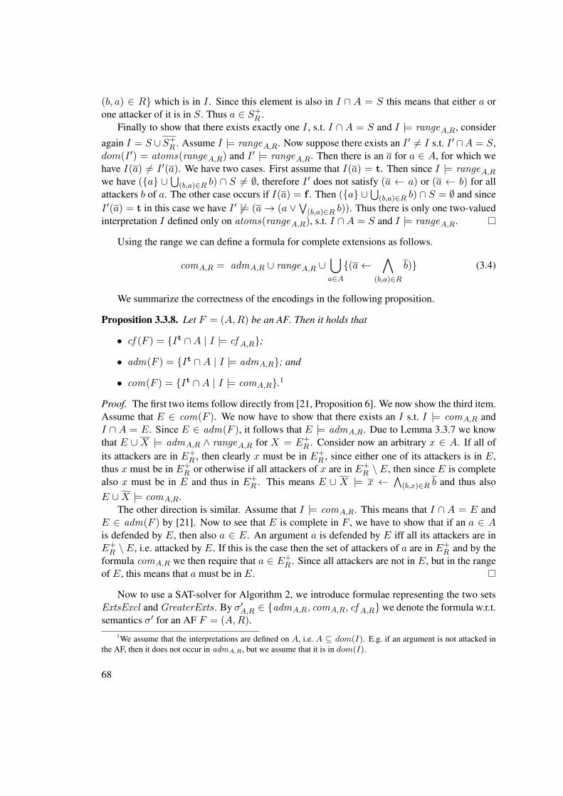
(b, a) ∈ R} which is in I . Since this element is also in I ∩ A = S this means that either a orone attacker of it is in S. Thus a ∈ S+

R .Finally to show that there exists exactly one I , s.t. I ∩ A = S and I |= rangeA,R, consider

again I = S ∪S+R . Assume I |= rangeA,R. Now suppose there exists an I ′ 6= I s.t. I ′ ∩A = S,

dom(I ′) = atoms(rangeA,R) and I ′ |= rangeA,R. Then there is an a for a ∈ A, for which wehave I(a) 6= I ′(a). We have two cases. First assume that I(a) = t. Then since I |= rangeA,Rwe have ({a} ∪⋃(b,a)∈R b) ∩ S 6= ∅, therefore I ′ does not satisfy (a ← a) or (a ← b) for allattackers b of a. The other case occurs if I(a) = f . Then ({a} ∪⋃(b,a)∈R b) ∩ S = ∅ and sinceI ′(a) = t in this case we have I ′ 6|= (a→ (a ∨∨(b,a)∈R b)). Thus there is only one two-valuedinterpretation I defined only on atoms(rangeA,R), s.t. I ∩A = S and I |= rangeA,R.

Using the range we can define a formula for complete extensions as follows.

comA,R = admA,R ∪ rangeA,R ∪⋃a∈A{(a←

∧(b,a)∈R

b)} (3.4)

We summarize the correctness of the encodings in the following proposition.

Proposition 3.3.8. Let F = (A,R) be an AF. Then it holds that

• cf (F ) = {It ∩A | I |= cf A,R};

• adm(F ) = {It ∩A | I |= admA,R}; and

• com(F ) = {It ∩A | I |= comA,R}.1

Proof. The first two items follow directly from [21, Proposition 6]. We now show the third item.Assume that E ∈ com(F ). We now have to show that there exists an I s.t. I |= comA,R andI ∩ A = E. Since E ∈ adm(F ), it follows that E |= admA,R. Due to Lemma 3.3.7 we knowthat E ∪ X |= admA,R ∧ rangeA,R for X = E+

R . Consider now an arbitrary x ∈ A. If all ofits attackers are in E+

R , then clearly x must be in E+R , since either one of its attackers is in E,

thus x must be in E+R or otherwise if all attackers of x are in E+

R \ E, then since E is completealso x must be in E and thus in E+

R . This means E ∪ X |= x ← ∧(b,x)∈R b and thus also

E ∪X |= comA,R.The other direction is similar. Assume that I |= comA,R. This means that I ∩ A = E and

E ∈ adm(F ) by [21]. Now to see that E is complete in F , we have to show that if an a ∈ Ais defended by E, then also a ∈ E. An argument a is defended by E iff all its attackers are inE+R \E, i.e. attacked by E. If this is the case then the set of attackers of a are in E+

R and by theformula comA,R we then require that a ∈ E+

R . Since all attackers are not in E, but in the rangeof E, this means that a must be in E.

Now to use a SAT-solver for Algorithm 2, we introduce formulae representing the two setsExtsExcl and GreaterExts . By σ′A,R ∈ {admA,R, comA,R, cf A,R}we denote the formula w.r.t.semantics σ′ for an AF F = (A,R).

1We assume that the interpretations are defined on A, i.e. A ⊆ dom(I). E.g. if an argument is not attacked inthe AF, then it does not occur in admA,R, but we assume that it is in dom(I).

68

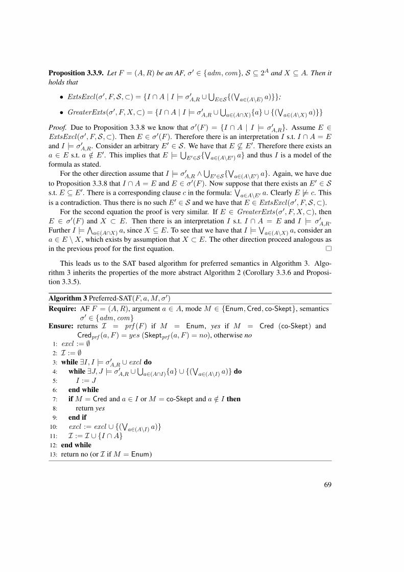
Proposition 3.3.9. Let F = (A,R) be an AF, σ′ ∈ {adm, com}, S ⊆ 2A and X ⊆ A. Then itholds that

• ExtsExcl(σ′, F,S,⊂) = {I ∩A | I |= σ′A,R ∪⋃E∈S{(

∨a∈(A\E) a)}};

• GreaterExts(σ′, F,X,⊂) = {I ∩A | I |= σ′A,R ∪⋃a∈(A∩X){a} ∪ {(

∨a∈(A\X) a)}}

Proof. Due to Proposition 3.3.8 we know that σ′(F ) = {I ∩ A | I |= σ′A,R}. Assume E ∈ExtsExcl(σ′, F,S,⊂). Then E ∈ σ′(F ). Therefore there is an interpretation I s.t. I ∩ A = Eand I |= σ′A,R. Consider an arbitrary E′ ∈ S. We have that E 6⊆ E′. Therefore there exists ana ∈ E s.t. a /∈ E′. This implies that E |= ⋃

E′∈S{∨a∈(A\E′) a} and thus I is a model of the

formula as stated.For the other direction assume that I |= σ′A,R ∧

⋃E′∈S{

∨a∈(A\E′) a}. Again, we have due

to Proposition 3.3.8 that I ∩ A = E and E ∈ σ′(F ). Now suppose that there exists an E′ ∈ Ss.t. E ⊆ E′. There is a corresponding clause c in the formula:

∨a∈A\E′ a. Clearly E 6|= c. This

is a contradiction. Thus there is no such E′ ∈ S and we have that E ∈ ExtsExcl(σ′, F,S,⊂).For the second equation the proof is very similar. If E ∈ GreaterExts(σ′, F,X,⊂), then

E ∈ σ′(F ) and X ⊂ E. Then there is an interpretation I s.t. I ∩ A = E and I |= σ′A,R.Further I |= ∧

a∈(A∩X) a, since X ⊆ E. To see that we have that I |= ∨a∈(A\X) a, consider an

a ∈ E \X , which exists by assumption that X ⊂ E. The other direction proceed analogous asin the previous proof for the first equation.

This leads us to the SAT based algorithm for preferred semantics in Algorithm 3. Algo-rithm 3 inherits the properties of the more abstract Algorithm 2 (Corollary 3.3.6 and Proposi-tion 3.3.5).

Algorithm 3 Preferred-SAT(F, a,M, σ′)


Ensure: returns I = prf (F ) if M = Enum, yes if M = Cred (co-Skept) andCredprf (a, F ) = yes (Skeptprf (a, F ) = no), otherwise no

1: excl := ∅2: I := ∅3: while ∃I, I |= σ′A,R ∪ excl do4: while ∃J, J |= σ′A,R ∪

⋃a∈(A∩I){a} ∪ {(

∨a∈(A\I) a)} do

5: I := J6: end while7: if M = Cred and a ∈ I or M = co-Skept and a /∈ I then8: return yes9: end if

10: excl := excl ∪ {(∨a∈(A\I) a)}11: I := I ∪ {I ∩A}12: end while13: return no (or I if M = Enum)

69

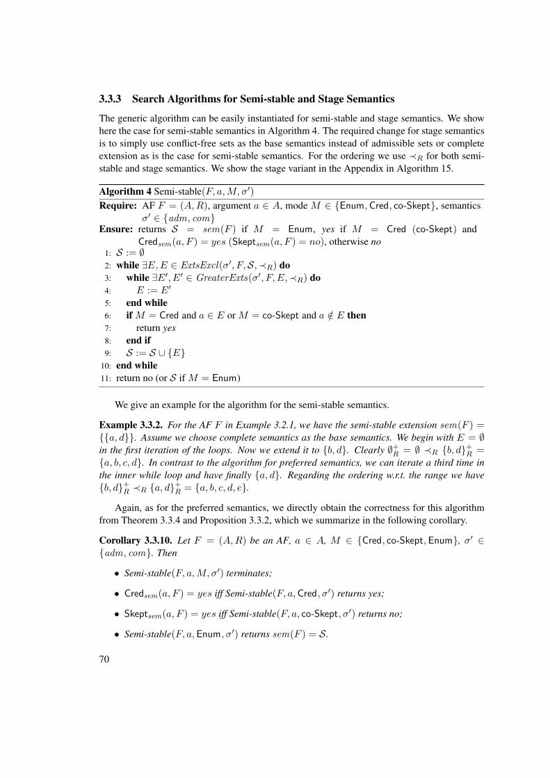
3.3.3 Search Algorithms for Semi-stable and Stage Semantics

The generic algorithm can be easily instantiated for semi-stable and stage semantics. We showhere the case for semi-stable semantics in Algorithm 4. The required change for stage semanticsis to simply use conflict-free sets as the base semantics instead of admissible sets or completeextension as is the case for semi-stable semantics. For the ordering we use ≺R for both semi-stable and stage semantics. We show the stage variant in the Appendix in Algorithm 15.

Algorithm 4 Semi-stable(F, a,M, σ′)


Ensure: returns S = sem(F ) if M = Enum, yes if M = Cred (co-Skept) andCredsem(a, F ) = yes (Skeptsem(a, F ) = no), otherwise no

1: S := ∅2: while ∃E,E ∈ ExtsExcl(σ′, F,S,≺R) do3: while ∃E′, E′ ∈ GreaterExts(σ′, F, E,≺R) do4: E := E′



We give an example for the algorithm for the semi-stable semantics.

Example 3.3.2. For the AF F in Example 3.2.1, we have the semi-stable extension sem(F ) ={{a, d}}. Assume we choose complete semantics as the base semantics. We begin with E = ∅in the first iteration of the loops. Now we extend it to {b, d}. Clearly ∅+R = ∅ ≺R {b, d}+R ={a, b, c, d}. In contrast to the algorithm for preferred semantics, we can iterate a third time inthe inner while loop and have finally {a, d}. Regarding the ordering w.r.t. the range we have{b, d}+R ≺R {a, d}+R = {a, b, c, d, e}.

Again, as for the preferred semantics, we directly obtain the correctness for this algorithmfrom Theorem 3.3.4 and Proposition 3.3.2, which we summarize in the following corollary.

Corollary 3.3.10. Let F = (A,R) be an AF, a ∈ A, M ∈ {Cred, co-Skept,Enum}, σ′ ∈{adm, com}. Then

• Semi-stable(F, a,M, σ′) terminates;

• Credsem(a, F ) = yes iff Semi-stable(F, a,Cred, σ′) returns yes;

• Skeptsem(a, F ) = yes iff Semi-stable(F, a, co-Skept, σ′) returns no;

• Semi-stable(F, a,Enum, σ′) returns sem(F ) = S.

70

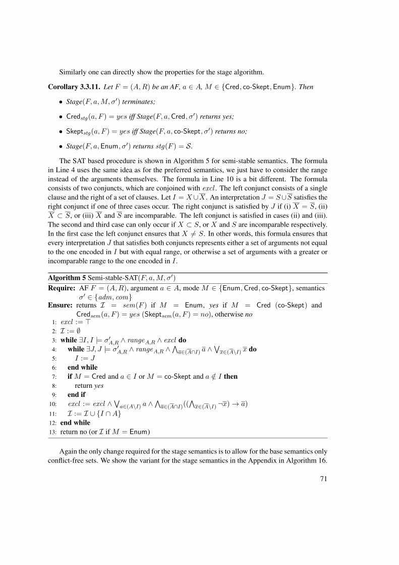
Similarly one can directly show the properties for the stage algorithm.

Corollary 3.3.11. Let F = (A,R) be an AF, a ∈ A, M ∈ {Cred, co-Skept,Enum}. Then

• Stage(F, a,M, σ′) terminates;

• Credstg(a, F ) = yes iff Stage(F, a,Cred, σ′) returns yes;

• Skeptstg(a, F ) = yes iff Stage(F, a, co-Skept, σ′) returns no;

• Stage(F, a,Enum, σ′) returns stg(F ) = S.

The SAT based procedure is shown in Algorithm 5 for semi-stable semantics. The formulain Line 4 uses the same idea as for the preferred semantics, we just have to consider the rangeinstead of the arguments themselves. The formula in Line 10 is a bit different. The formulaconsists of two conjuncts, which are conjoined with excl . The left conjunct consists of a singleclause and the right of a set of clauses. Let I = X∪X . An interpretation J = S∪S satisfies theright conjunct if one of three cases occur. The right conjunct is satisfied by J if (i) X = S, (ii)X ⊂ S, or (iii) X and S are incomparable. The left conjunct is satisfied in cases (ii) and (iii).The second and third case can only occur if X ⊂ S, or X and S are incomparable respectively.In the first case the left conjunct ensures that X 6= S. In other words, this formula ensures thatevery interpretation J that satisfies both conjuncts represents either a set of arguments not equalto the one encoded in I but with equal range, or otherwise a set of arguments with a greater orincomparable range to the one encoded in I .

Algorithm 5 Semi-stable-SAT(F, a,M, σ′)


Ensure: returns I = sem(F ) if M = Enum, yes if M = Cred (co-Skept) andCredsem(a, F ) = yes (Skeptsem(a, F ) = no), otherwise no

1: excl := >2: I := ∅3: while ∃I, I |= σ′A,R ∧ rangeA,R ∧ excl do4: while ∃J, J |= σ′A,R ∧ rangeA,R ∧

∧a∈(A∩I) a ∧

∨x∈(A\I) x do


10: excl := excl ∧∨a∈(A\I) a ∧∧a∈(A∩I)((

∧x∈(A\I) ¬x)→ a)

11: I := I ∪ {I ∩A}12: end while13: return no (or I if M = Enum)

Again the only change required for the stage semantics is to allow for the base semantics onlyconflict-free sets. We show the variant for the stage semantics in the Appendix in Algorithm 16.

71

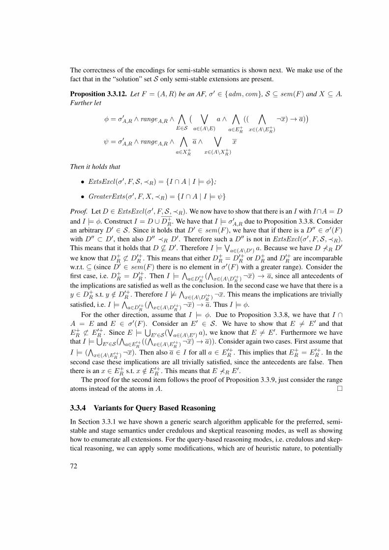
The correctness of the encodings for semi-stable semantics is shown next. We make use of thefact that in the “solution” set S only semi-stable extensions are present.

Proposition 3.3.12. Let F = (A,R) be an AF, σ′ ∈ {adm, com}, S ⊆ sem(F ) and X ⊆ A.Further let

φ = σ′A,R ∧ rangeA,R ∧∧E∈S

( ∨a∈(A\E)

a ∧∧a∈E+

R

((∧

x∈(A\E+R )

¬x)→ a))

ψ = σ′A,R ∧ rangeA,R ∧∧

a∈X+R

a ∧∨

x∈(A\X+R )

x

Then it holds that

• ExtsExcl(σ′, F,S,≺R) = {I ∩A | I |= φ};

• GreaterExts(σ′, F,X,≺R) = {I ∩A | I |= ψ}

Proof. LetD ∈ ExtsExcl(σ′, F,S,≺R). We now have to show that there is an I with I∩A = D

and I |= φ. Construct I = D ∪D+R . We have that I |= σ′A,R due to Proposition 3.3.8. Consider

an arbitrary D′ ∈ S . Since it holds that D′ ∈ sem(F ), we have that if there is a D′′ ∈ σ′(F )with D′′ ⊂ D′, then also D′′ ≺R D′. Therefore such a D′′ is not in ExtsExcl(σ′, F,S,≺R).This means that it holds that D 6⊆ D′. Therefore I |= ∨a∈(A\D′) a. Because we have D 6≺R D′we know that D+

R 6⊂ D′+R . This means that either D+R = D′+R or D+

R and D′+R are incomparablew.r.t. ⊆ (since D′ ∈ sem(F ) there is no element in σ′(F ) with a greater range). Consider thefirst case, i.e. D+

R = D′+R . Then I |= ∧a∈D′+R

(∧x∈(A\D′+R ) ¬x) → a, since all antecedents of

the implications are satisfied as well as the conclusion. In the second case we have that there is ay ∈ D+

R s.t. y /∈ D′+R . Therefore I 6|= ∧x∈(A\D′+R ) ¬x. This means the implications are trivially

satisfied, i.e. I |= ∧a∈D′+R(∧x∈(A\D′+R ) ¬x)→ a. Thus I |= φ.

For the other direction, assume that I |= φ. Due to Proposition 3.3.8, we have that I ∩A = E and E ∈ σ′(F ). Consider an E′ ∈ S. We have to show that E 6= E′ and thatE+R 6⊂ E′+R . Since E |= ⋃

E′∈S(∨a∈(A\E′) a), we know that E 6= E′. Furthermore we have

that I |= ⋃E′∈S(∧a∈E′+R

((∧x∈(A\E′+R ) ¬x)→ a)). Consider again two cases. First assume that

I |= (∧x∈(A\E′+R ) ¬x). Then also a ∈ I for all a ∈ E′+R . This implies that E+

R = E′+R . In thesecond case these implications are all trivially satisfied, since the antecedents are false. Thenthere is an x ∈ E+

R s.t. x /∈ E′+R . This means that E 6≺R E′.The proof for the second item follows the proof of Proposition 3.3.9, just consider the range

atoms instead of the atoms in A.

3.3.4 Variants for Query Based Reasoning

In Section 3.3.1 we have shown a generic search algorithm applicable for the preferred, semi-stable and stage semantics under credulous and skeptical reasoning modes, as well as showinghow to enumerate all extensions. For the query-based reasoning modes, i.e. credulous and skep-tical reasoning, we can apply some modifications, which are of heuristic nature, to potentially

72

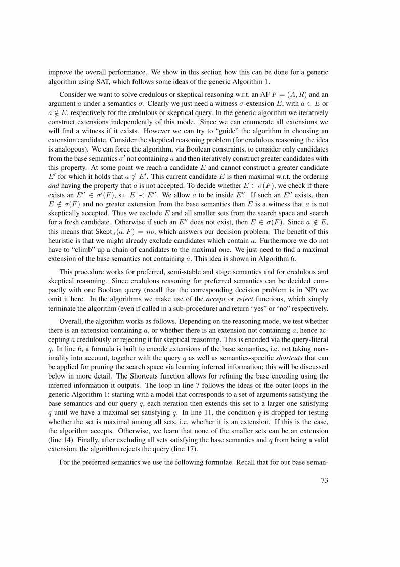
improve the overall performance. We show in this section how this can be done for a genericalgorithm using SAT, which follows some ideas of the generic Algorithm 1.

Consider we want to solve credulous or skeptical reasoning w.r.t. an AF F = (A,R) and anargument a under a semantics σ. Clearly we just need a witness σ-extension E, with a ∈ E ora /∈ E, respectively for the credulous or skeptical query. In the generic algorithm we iterativelyconstruct extensions independently of this mode. Since we can enumerate all extensions wewill find a witness if it exists. However we can try to “guide” the algorithm in choosing anextension candidate. Consider the skeptical reasoning problem (for credulous reasoning the ideais analogous). We can force the algorithm, via Boolean constraints, to consider only candidatesfrom the base semantics σ′ not containing a and then iteratively construct greater candidates withthis property. At some point we reach a candidate E and cannot construct a greater candidateE′ for which it holds that a /∈ E′. This current candidate E is then maximal w.r.t. the orderingand having the property that a is not accepted. To decide whether E ∈ σ(F ), we check if thereexists an E′′ ∈ σ′(F ), s.t. E ≺ E′′. We allow a to be inside E′′. If such an E′′ exists, thenE /∈ σ(F ) and no greater extension from the base semantics than E is a witness that a is notskeptically accepted. Thus we exclude E and all smaller sets from the search space and searchfor a fresh candidate. Otherwise if such an E′′ does not exist, then E ∈ σ(F ). Since a /∈ E,this means that Skeptσ(a, F ) = no, which answers our decision problem. The benefit of thisheuristic is that we might already exclude candidates which contain a. Furthermore we do nothave to “climb” up a chain of candidates to the maximal one. We just need to find a maximalextension of the base semantics not containing a. This idea is shown in Algorithm 6.

This procedure works for preferred, semi-stable and stage semantics and for credulous andskeptical reasoning. Since credulous reasoning for preferred semantics can be decided com-pactly with one Boolean query (recall that the corresponding decision problem is in NP) weomit it here. In the algorithms we make use of the accept or reject functions, which simplyterminate the algorithm (even if called in a sub-procedure) and return “yes” or “no” respectively.

Overall, the algorithm works as follows. Depending on the reasoning mode, we test whetherthere is an extension containing a, or whether there is an extension not containing a, hence ac-cepting a credulously or rejecting it for skeptical reasoning. This is encoded via the query-literalq. In line 6, a formula is built to encode extensions of the base semantics, i.e. not taking max-imality into account, together with the query q as well as semantics-specific shortcuts that canbe applied for pruning the search space via learning inferred information; this will be discussedbelow in more detail. The Shortcuts function allows for refining the base encoding using theinferred information it outputs. The loop in line 7 follows the ideas of the outer loops in thegeneric Algorithm 1: starting with a model that corresponds to a set of arguments satisfying thebase semantics and our query q, each iteration then extends this set to a larger one satisfyingq until we have a maximal set satisfying q. In line 11, the condition q is dropped for testingwhether the set is maximal among all sets, i.e. whether it is an extension. If this is the case,the algorithm accepts. Otherwise, we learn that none of the smaller sets can be an extension(line 14). Finally, after excluding all sets satisfying the base semantics and q from being a validextension, the algorithm rejects the query (line 17).

For the preferred semantics we use the following formulae. Recall that for our base seman-

73

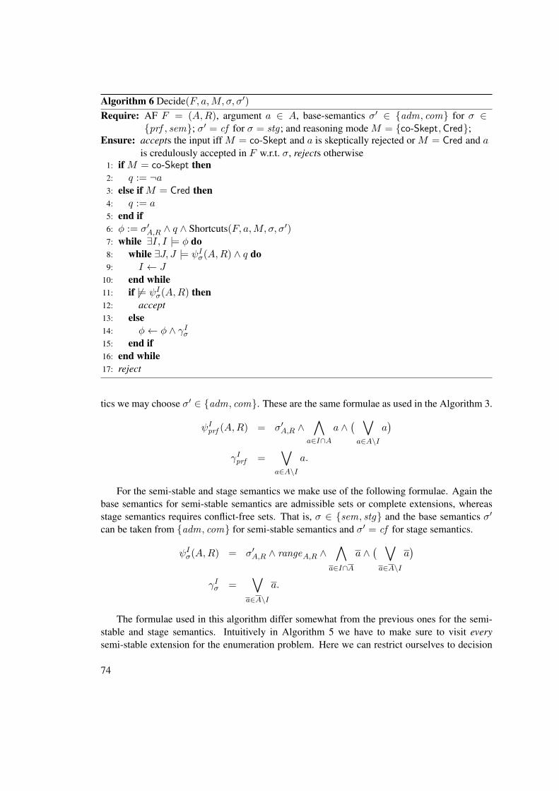
Algorithm 6 Decide(F, a,M, σ, σ′)

Require: AF F = (A,R), argument a ∈ A, base-semantics σ′ ∈ {adm, com} for σ ∈{prf , sem}; σ′ = cf for σ = stg ; and reasoning mode M = {co-Skept,Cred};

Ensure: accepts the input iff M = co-Skept and a is skeptically rejected or M = Cred and ais credulously accepted in F w.r.t. σ, rejects otherwise

1: if M = co-Skept then2: q := ¬a3: else if M = Cred then4: q := a5: end if6: φ := σ′A,R ∧ q ∧ Shortcuts(F, a,M, σ, σ′)7: while ∃I, I |= φ do8: while ∃J, J |= ψIσ(A,R) ∧ q do9: I ← J

10: end while11: if 6|= ψIσ(A,R) then12: accept13: else14: φ← φ ∧ γIσ15: end if16: end while17: reject

tics we may choose σ′ ∈ {adm, com}. These are the same formulae as used in the Algorithm 3.

ψIprf (A,R) = σ′A,R ∧∧

a∈I∩Aa ∧

( ∨a∈A\I

a)

γIprf =∨

a∈A\I

a.

For the semi-stable and stage semantics we make use of the following formulae. Again thebase semantics for semi-stable semantics are admissible sets or complete extensions, whereasstage semantics requires conflict-free sets. That is, σ ∈ {sem, stg} and the base semantics σ′

can be taken from {adm, com} for semi-stable semantics and σ′ = cf for stage semantics.

ψIσ(A,R) = σ′A,R ∧ rangeA,R ∧∧

a∈I∩A

a ∧( ∨a∈A\I

a)

γIσ =∨

a∈A\I

a.

The formulae used in this algorithm differ somewhat from the previous ones for the semi-stable and stage semantics. Intuitively in Algorithm 5 we have to make sure to visit everysemi-stable extension for the enumeration problem. Here we can restrict ourselves to decision

74

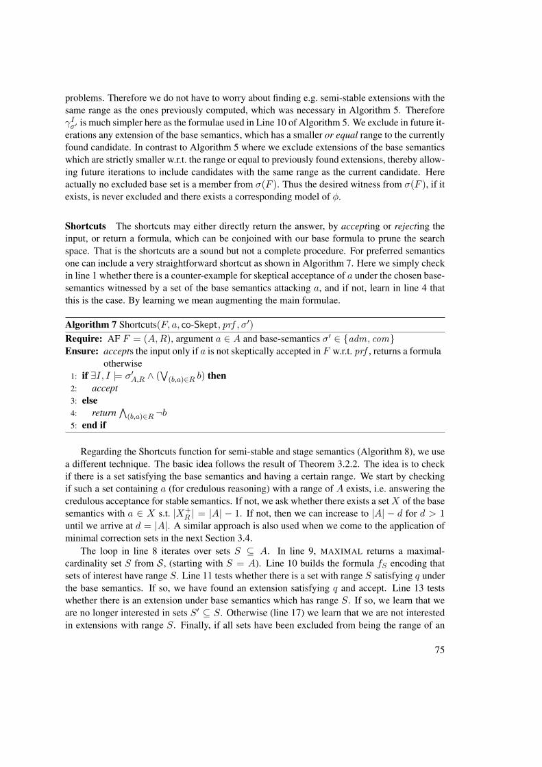
problems. Therefore we do not have to worry about finding e.g. semi-stable extensions with thesame range as the ones previously computed, which was necessary in Algorithm 5. ThereforeγIσ′ is much simpler here as the formulae used in Line 10 of Algorithm 5. We exclude in future it-erations any extension of the base semantics, which has a smaller or equal range to the currentlyfound candidate. In contrast to Algorithm 5 where we exclude extensions of the base semanticswhich are strictly smaller w.r.t. the range or equal to previously found extensions, thereby allow-ing future iterations to include candidates with the same range as the current candidate. Hereactually no excluded base set is a member from σ(F ). Thus the desired witness from σ(F ), if itexists, is never excluded and there exists a corresponding model of φ.

Shortcuts The shortcuts may either directly return the answer, by accepting or rejecting theinput, or return a formula, which can be conjoined with our base formula to prune the searchspace. That is the shortcuts are a sound but not a complete procedure. For preferred semanticsone can include a very straightforward shortcut as shown in Algorithm 7. Here we simply checkin line 1 whether there is a counter-example for skeptical acceptance of a under the chosen base-semantics witnessed by a set of the base semantics attacking a, and if not, learn in line 4 thatthis is the case. By learning we mean augmenting the main formulae.

Algorithm 7 Shortcuts(F, a, co-Skept, prf , σ′)Require: AF F = (A,R), argument a ∈ A and base-semantics σ′ ∈ {adm, com}Ensure: accepts the input only if a is not skeptically accepted in F w.r.t. prf , returns a formula

otherwise1: if ∃I, I |= σ′A,R ∧ (

∨(b,a)∈R b) then

2: accept3: else4: return

∧(b,a)∈R ¬b

5: end if

Regarding the Shortcuts function for semi-stable and stage semantics (Algorithm 8), we usea different technique. The basic idea follows the result of Theorem 3.2.2. The idea is to checkif there is a set satisfying the base semantics and having a certain range. We start by checkingif such a set containing a (for credulous reasoning) with a range of A exists, i.e. answering thecredulous acceptance for stable semantics. If not, we ask whether there exists a setX of the basesemantics with a ∈ X s.t. |X+

R | = |A| − 1. If not, then we can increase to |A| − d for d > 1until we arrive at d = |A|. A similar approach is also used when we come to the application ofminimal correction sets in the next Section 3.4.

The loop in line 8 iterates over sets S ⊆ A. In line 9, MAXIMAL returns a maximal-cardinality set S from S , (starting with S = A). Line 10 builds the formula fS encoding thatsets of interest have range S. Line 11 tests whether there is a set with range S satisfying q underthe base semantics. If so, we have found an extension satisfying q and accept. Line 13 testswhether there is an extension under base semantics which has range S. If so, we learn that weare no longer interested in sets S′ ⊆ S. Otherwise (line 17) we learn that we are not interestedin extensions with range S. Finally, if all sets have been excluded from being the range of an

75

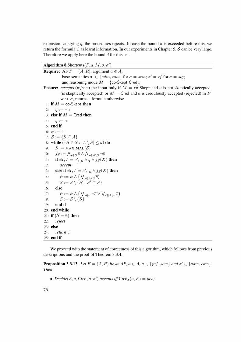
extension satisfying q, the procedures rejects. In case the bound d is exceeded before this, wereturn the formula ψ as learnt information. In our experiments in Chapter 5, S can be very large.Therefore we apply here the bound d for this set.

Algorithm 8 Shortcuts(F, a,M, σ, σ′)

Require: AF F = (A,R), argument a ∈ A,base-semantics σ′ ∈ {adm, com} for σ = sem; σ′ = cf for σ = stg ;and reasoning mode M = {co-Skept,Cred};

Ensure: accepts (rejects) the input only if M = co-Skept and a is not skeptically accepted(is skeptically accepted) or M = Cred and a is credulously accepted (rejected) in Fw.r.t. σ, returns a formula otherwise

1: if M = co-Skept then2: q := ¬a3: else if M = Cred then4: q := a5: end if6: ψ := >7: S := {S ⊆ A}8: while (∃S ∈ S : |A \ S| ≤ d) do9: S := MAXIMAL(S)

10: fS :=∧s∈S s ∧

∧s∈A\S ¬s

11: if ∃I, I |= σ′A,R ∧ q ∧ fS(X) then12: accept13: else if ∃I, I |= σ′A,R ∧ fS(X) then14: ψ := ψ ∧

(∨s∈A\S s

)15: S := S \ {S′ | S′ ⊂ S}16: else17: ψ := ψ ∧

(∨s∈S ¬s ∨

∨s∈A\S s

)18: S := S \ {S}19: end if20: end while21: if (S = ∅) then22: reject23: else24: return ψ25: end if

We proceed with the statement of correctness of this algorithm, which follows from previousdescriptions and the proof of Theorem 3.3.4.

Proposition 3.3.13. Let F = (A,R) be an AF, a ∈ A, σ ∈ {prf , sem} and σ′ ∈ {adm, com}.Then

• Decide(F, a,Cred, σ, σ′) accepts iff Credσ(a, F ) = yes;

76

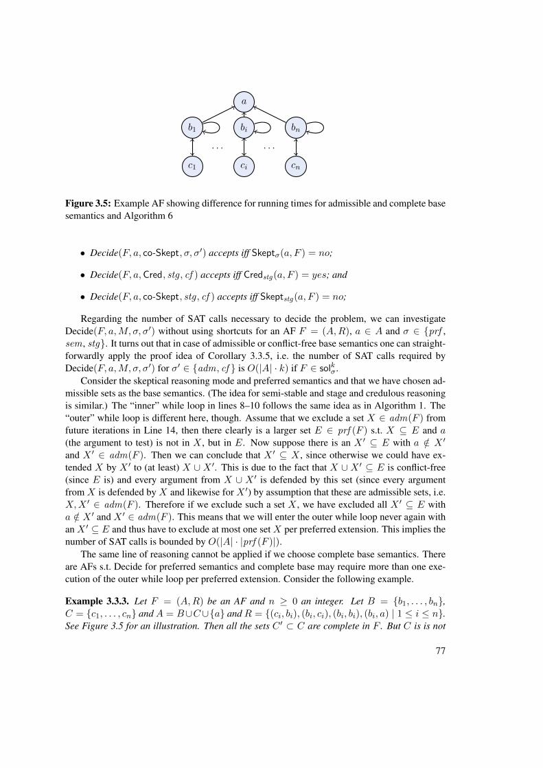
a

b1

c1

· · ·

bi

ci

· · ·

bn

cn

Figure 3.5: Example AF showing difference for running times for admissible and complete basesemantics and Algorithm 6

• Decide(F, a, co-Skept, σ, σ′) accepts iff Skeptσ(a, F ) = no;

• Decide(F, a,Cred, stg , cf ) accepts iff Credstg(a, F ) = yes; and

• Decide(F, a, co-Skept, stg , cf ) accepts iff Skeptstg(a, F ) = no;

Regarding the number of SAT calls necessary to decide the problem, we can investigateDecide(F, a,M, σ, σ′) without using shortcuts for an AF F = (A,R), a ∈ A and σ ∈ {prf ,sem , stg}. It turns out that in case of admissible or conflict-free base semantics one can straight-forwardly apply the proof idea of Corollary 3.3.5, i.e. the number of SAT calls required byDecide(F, a,M, σ, σ′) for σ′ ∈ {adm, cf } is O(|A| · k) if F ∈ solkσ.

Consider the skeptical reasoning mode and preferred semantics and that we have chosen ad-missible sets as the base semantics. (The idea for semi-stable and stage and credulous reasoningis similar.) The “inner” while loop in lines 8–10 follows the same idea as in Algorithm 1. The“outer” while loop is different here, though. Assume that we exclude a set X ∈ adm(F ) fromfuture iterations in Line 14, then there clearly is a larger set E ∈ prf (F ) s.t. X ⊆ E and a(the argument to test) is not in X , but in E. Now suppose there is an X ′ ⊆ E with a /∈ X ′

and X ′ ∈ adm(F ). Then we can conclude that X ′ ⊆ X , since otherwise we could have ex-tended X by X ′ to (at least) X ∪ X ′. This is due to the fact that X ∪ X ′ ⊆ E is conflict-free(since E is) and every argument from X ∪ X ′ is defended by this set (since every argumentfrom X is defended by X and likewise for X ′) by assumption that these are admissible sets, i.e.X,X ′ ∈ adm(F ). Therefore if we exclude such a set X , we have excluded all X ′ ⊆ E witha /∈ X ′ and X ′ ∈ adm(F ). This means that we will enter the outer while loop never again withan X ′ ⊆ E and thus have to exclude at most one set X per preferred extension. This implies thenumber of SAT calls is bounded by O(|A| · |prf (F )|).

The same line of reasoning cannot be applied if we choose complete base semantics. Thereare AFs s.t. Decide for preferred semantics and complete base may require more than one exe-cution of the outer while loop per preferred extension. Consider the following example.

Example 3.3.3. Let F = (A,R) be an AF and n ≥ 0 an integer. Let B = {b1, . . . , bn},C = {c1, . . . , cn} andA = B∪C∪{a} andR = {(ci, bi), (bi, ci), (bi, bi), (bi, a) | 1 ≤ i ≤ n}.See Figure 3.5 for an illustration. Then all the sets C ′ ⊂ C are complete in F . But C is is not

77

complete in F , since a is defended by C in F . The set C is however admissible in F . Theonly preferred extension of F is C ∪ {a}. If we now apply Algorithm 6 to this framework withthe admissible base semantics and checking if a is not skeptically accepted, then it computesC in the inner while loop as the first admissible set to exclude from our search space. Afterthat the algorithm immediately terminates. For the complete base semantics we have a differentpicture, since if the inner while loop terminates we exclude just one set C \ {cj} from the searchspace and may re-enter the loops with a fresh candidate containing cj . Therefore for only onepreferred extension, we enter the outer while loop n times in this example.

We point out that the complete base semantics is nevertheless useful as seen in the empiricalevaluation in Section 5, where the complete base outperformed the admissible base on certainAFs.

3.4 Utilizing Minimal Correction Sets and Backbones

In this section we present algorithms to solve reasoning problems associated with several com-putationally complex semantics on AFs, namely the semi-stable, stage, eager, stage-ideal andideal semantics using SAT-extensions. We apply sophisticated algorithms for minimal correc-tion sets (MCSes) to solve reasoning tasks under the semi-stable and stage semantics, in particu-lar AllSkeptsem and AllSkeptstg , and procedures for computing backbones to solve AllCredadm .The systems we use for computing MCSes or backbones rely on iterative calls to a SAT-solver.

The eager semantics is based on the semi-stable semantics and, given the skeptically ac-cepted arguments under the semi-stable semantics from the MCS algorithm, one can computethe unique eager extension in polynomial time by means of a post-processing step. Similarly onecan apply this technique for the unique stage-ideal extension. The algorithm behind the idealsemantics is more complicated and is taken from [67]. The difficult part of this algorithm froma computational point of view is to compute AllCredadm ; the remainder can be done by a similarpost-processing technique as for eager.

In the following we show how this works in detail. We start with a formal introduction toMCSes and backbones in Section 3.4.1. In Section 3.4.2 we show how to use MCSes to computethe semi-stable and stage extensions, in Section 3.4.3 how to use this result to compute the eagerand stage-ideal extension. In Section 3.4.4 we show how to utilize backbones to compute theideal extensions of a given framework. In all cases we build on existing reductions to SAT forthe admissible and stable semantics [21].

3.4.1 SAT Extensions

In some applications encountering an unsatisfiable formula is common. However one might stillbe interested in partially satisfying a formula then. For instance some of the constraints encodedas clauses might not be necessary for a solution. In particular one can think of the concept ofhard and soft constraints (or clauses), which denote constraints which have to be satisfied or notrespectively. This is captured e.g. in the following definition for MCSes. Recall that if a formulais in CNF, then we can view it as a set of clauses, each containing a set of literals.

78

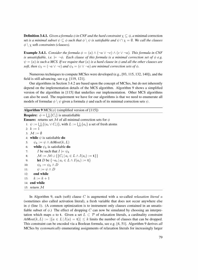
Definition 3.4.1. Given a formula φ in CNF and the hard constraint χ ⊆ φ, a minimal correctionset is a minimal subset ψ ⊆ φ such that φ \ ψ is satisfiable and ψ ∩ χ = ∅. We call the clausesφ \ χ soft constraints (clauses).

Example 3.4.1. Consider the formula φ = (a) ∧ (¬a ∨ ¬c) ∧ (c ∨ ¬a). This formula in CNFis unsatisfiable, i.e. |= ¬φ. Each clause of this formula is a minimal correction set of φ e.g.ψ = (a) is such a MCS. If we require that (a) is a hard clause in φ and all the other clauses aresoft, then ψ2 = (¬a ∨ ¬c) and ψ3 = (c ∨ ¬a) are minimal correction sets of φ.

Numerous techniques to compute MCSes were developed (e.g., [93, 115, 132, 140]), and thefield is still advancing, see e.g. [119, 121].

Our algorithms in Section 3.4.2 are based upon the concept of MCSes, but do not inherentlydepend on the implementation details of the MCS algorithm. Algorithm 9 shows a simplifiedversion of the algorithm in [115] that underlies our implementation. Other MCS algorithmscan also be used. The requirement we have for our algorithms is that we need to enumerate allmodels of formulae φ \ ψ given a formula φ and each of its minimal correction sets ψ.

Algorithm 9 MCS(φ) (simplified version of [115])Require: φ =

⋃i{Ci} is unsatisfiable

Ensure: returns setM of all minimal correction sets for φ1: ψ :=

⋃i{(ai ∨ Ci)}, with L :=

⋃i{ai} a set of fresh atoms

2: k := 13: M := ∅4: while ψ is satisfiable do5: ψk := ψ ∧ AtMost(k, L)6: while ψk is satisfiable do7: I be such that I |= ψk8: M :=M∪ {{Ci | ai ∈ L ∧ I(ai) := t}}9: let D be {¬ai | ai ∈ L ∧ I(ai) := t}

10: ψk := ψk ∧D11: ψ := ψ ∧D12: end while13: k := k + 114: end while15: returnM

In Algorithm 9, each (soft) clause C is augmented with a so-called relaxation literal a(sometimes also called activation literal), a fresh variable that does not occur anywhere elsein φ (line 1). (A common optimization is to instrument only clauses contained in an unsatis-fiable subset of φ.) The effect of dropping C can now be simulated by choosing an interpre-tation which maps a to t. Given a set L ⊂ P of relaxation literals, a cardinality constraintAtMost(k, L) := |{a ∈ L | I(a) = t}| ≤ k limits the number of clauses that can be dropped.This constraint can be encoded via a Boolean formula, see e.g. [4, 51]. Algorithm 9 derives allMCSes by systematically enumerating assignments of relaxation literals for increasingly larger

79

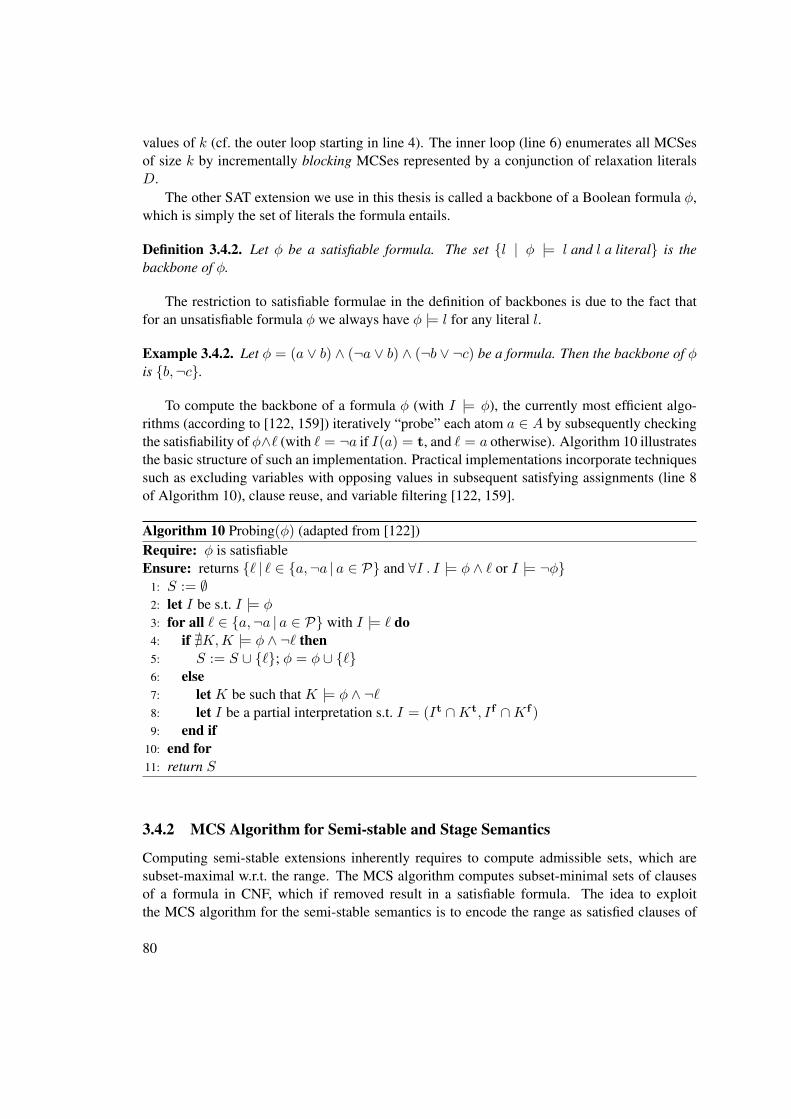
values of k (cf. the outer loop starting in line 4). The inner loop (line 6) enumerates all MCSesof size k by incrementally blocking MCSes represented by a conjunction of relaxation literalsD.

The other SAT extension we use in this thesis is called a backbone of a Boolean formula φ,which is simply the set of literals the formula entails.

Definition 3.4.2. Let φ be a satisfiable formula. The set {l | φ |= l and l a literal} is thebackbone of φ.

The restriction to satisfiable formulae in the definition of backbones is due to the fact thatfor an unsatisfiable formula φ we always have φ |= l for any literal l.

Example 3.4.2. Let φ = (a ∨ b) ∧ (¬a ∨ b) ∧ (¬b ∨ ¬c) be a formula. Then the backbone of φis {b,¬c}.

To compute the backbone of a formula φ (with I |= φ), the currently most efficient algo-rithms (according to [122, 159]) iteratively “probe” each atom a ∈ A by subsequently checkingthe satisfiability of φ∧` (with ` = ¬a if I(a) = t, and ` = a otherwise). Algorithm 10 illustratesthe basic structure of such an implementation. Practical implementations incorporate techniquessuch as excluding variables with opposing values in subsequent satisfying assignments (line 8of Algorithm 10), clause reuse, and variable filtering [122, 159].

Algorithm 10 Probing(φ) (adapted from [122])Require: φ is satisfiableEnsure: returns {` | ` ∈ {a,¬a | a ∈ P} and ∀I . I |= φ ∧ ` or I |= ¬φ}

1: S := ∅2: let I be s.t. I |= φ3: for all ` ∈ {a,¬a | a ∈ P} with I |= ` do4: if @K,K |= φ ∧ ¬` then5: S := S ∪ {`}; φ = φ ∪ {`}6: else7: let K be such that K |= φ ∧ ¬`8: let I be a partial interpretation s.t. I = (It ∩Kt, If ∩Kf )9: end if

10: end for11: return S

3.4.2 MCS Algorithm for Semi-stable and Stage Semantics

Computing semi-stable extensions inherently requires to compute admissible sets, which aresubset-maximal w.r.t. the range. The MCS algorithm computes subset-minimal sets of clausesof a formula in CNF, which if removed result in a satisfiable formula. The idea to exploitthe MCS algorithm for the semi-stable semantics is to encode the range as satisfied clauses of

80

a propositional formula for a given interpretation and additionally requiring that the result isadmissible.

For this to work we slightly adapt the formulae from [21] for the stable semantics. Given anAF F = (A,R) and a ∈ A we define the following formulae.

in_rangea,R = (a ∨∨

(b,a)∈R

b) (3.5)

all_in_rangeA,R =⋃a∈A

{in_rangea,R

}(3.6)

The formula in_rangea,R indicates whether the argument a is in the range w.r.t. the atomsset to true in an interpretation. In other words, for an AF F = (A,R) and a ∈ A we have,I |= in_rangea,R iff a ∈ S+

R for It = S. The formula all_in_rangeA,R is satisfied if allarguments are in the range. Note that this encoding of the range differs from previous formulae,where we encoded the range as variables set to true. We summarize this more formally in thefollowing lemma, which follows directly from definition of in_rangea,R.

Lemma 3.4.1. Let F = (A,R) be an AF, S ⊆ A, a ∈ A and I an interpretation on A. ThenI |= in_rangea,R iff a ∈ S+

R for It = S.

Conjoining the formulae admA,R and all_in_rangeA,R, which we denote by stbA,R, resultsin a formula equivalent to the stable formula in [21].

stbA,R = admA,R ∪ all_in_rangeA,R (3.7)

An interpretation I which satisfies admA,R for a given AF F = (A,R) and a subset-maximal set of clauses of all_in_rangeA,R corresponds to a semi-stable extension of F . Conse-quently, we can derive semi-stable extensions from the correction sets computed with the MCSalgorithm, as long as no clause from admA,R is dropped. That is, we consider the clauses ofthe formula admA,R as hard constraints and the clauses in all_in_rangeA,R as soft constraints.Note also, since any AF F = (A,R) has at least one admissible set, we know that admA,R is al-ways satisfiable. If stbA,R is satisfiable, meaning that F has stable extensions, then immediatelythis computation yields the stable extensions, which are equal to the semi-stable extensions inthis case.

The following proposition shows this result more formally. For a given propositional formulaφ in CNF and an interpretation I , we define φI to be the set of clauses in φ, which are satisfiedby I , i.e. φI := {C ∈ φ | I |= C}.

Proposition 3.4.2. Let F = (A,R) be an AF and Isem = {I | I |= admA,R and @I ′ : I ′ |=admA,R s.t. all_in_rangeIA,R ⊂ all_in_rangeI

′A,R}. Then sem(F ) = Isem .

Proof. Given an a ∈ A, by Lemma 3.4.1 we have that an interpretation I satisfies in_rangea,Riff a ∈ S+

R for It = S. Therefore all_in_rangeIA,R directly corresponds to S+R .

Let F = (A,R) be an AF. Assume E ∈ sem(F ), then define the following interpretationI with I(a) = t iff a ∈ E. Then I |= admA,R, since E is admissible by definition and due

81

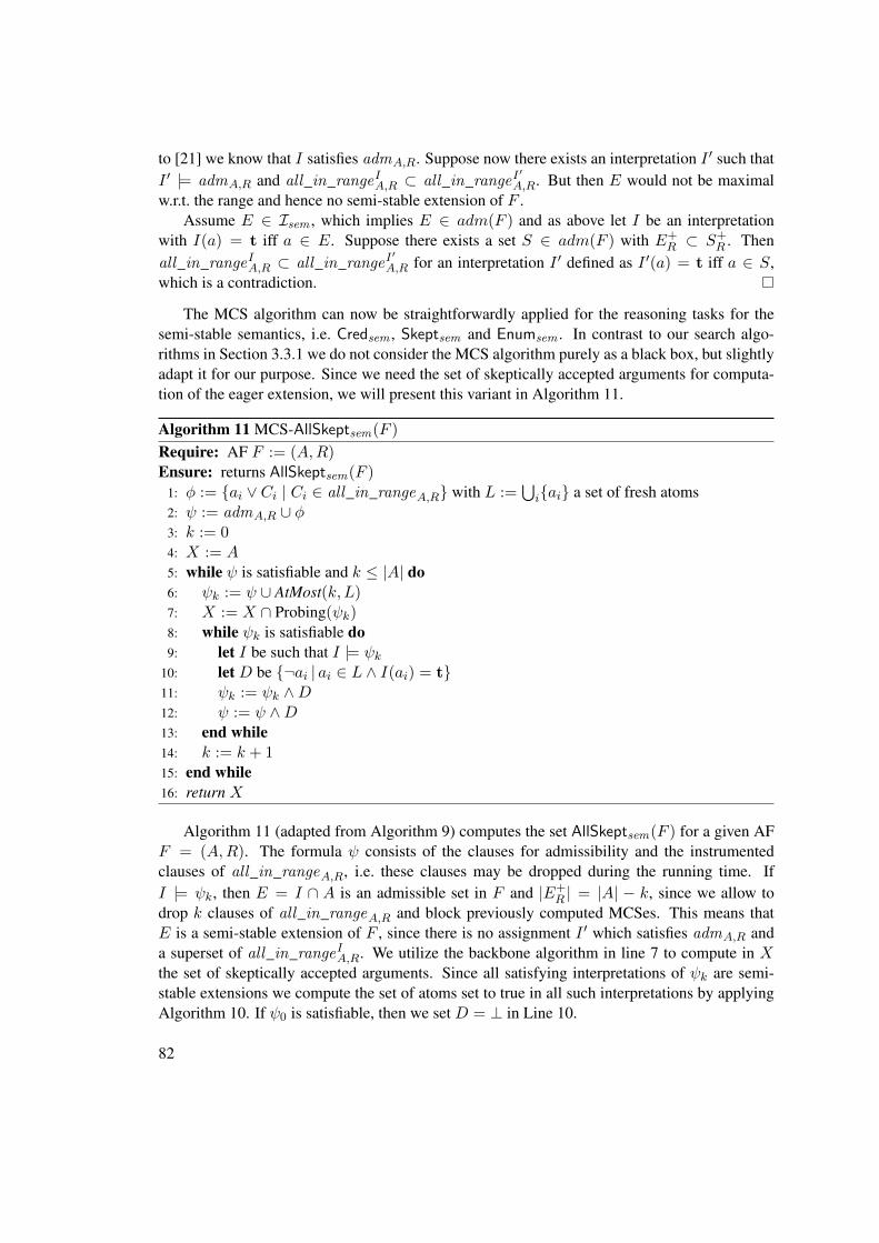
to [21] we know that I satisfies admA,R. Suppose now there exists an interpretation I ′ such thatI ′ |= admA,R and all_in_rangeIA,R ⊂ all_in_rangeI

′A,R. But then E would not be maximal

w.r.t. the range and hence no semi-stable extension of F .Assume E ∈ Isem , which implies E ∈ adm(F ) and as above let I be an interpretation

with I(a) = t iff a ∈ E. Suppose there exists a set S ∈ adm(F ) with E+R ⊂ S+

R . Thenall_in_rangeIA,R ⊂ all_in_rangeI

′A,R for an interpretation I ′ defined as I ′(a) = t iff a ∈ S,

which is a contradiction.

The MCS algorithm can now be straightforwardly applied for the reasoning tasks for thesemi-stable semantics, i.e. Credsem , Skeptsem and Enumsem . In contrast to our search algo-rithms in Section 3.3.1 we do not consider the MCS algorithm purely as a black box, but slightlyadapt it for our purpose. Since we need the set of skeptically accepted arguments for computa-tion of the eager extension, we will present this variant in Algorithm 11.

Algorithm 11 MCS-AllSkeptsem(F )

Require: AF F := (A,R)Ensure: returns AllSkeptsem(F )

1: φ := {ai ∨ Ci | Ci ∈ all_in_rangeA,R} with L :=⋃i{ai} a set of fresh atoms

2: ψ := admA,R ∪ φ3: k := 04: X := A5: while ψ is satisfiable and k ≤ |A| do6: ψk := ψ ∪ AtMost(k, L)7: X := X ∩ Probing(ψk)8: while ψk is satisfiable do9: let I be such that I |= ψk

10: let D be {¬ai | ai ∈ L ∧ I(ai) = t}11: ψk := ψk ∧D12: ψ := ψ ∧D13: end while14: k := k + 115: end while16: return X

Algorithm 11 (adapted from Algorithm 9) computes the set AllSkeptsem(F ) for a given AFF = (A,R). The formula ψ consists of the clauses for admissibility and the instrumentedclauses of all_in_rangeA,R, i.e. these clauses may be dropped during the running time. IfI |= ψk, then E = I ∩ A is an admissible set in F and |E+

R | = |A| − k, since we allow todrop k clauses of all_in_rangeA,R and block previously computed MCSes. This means thatE is a semi-stable extension of F , since there is no assignment I ′ which satisfies admA,R anda superset of all_in_rangeIA,R. We utilize the backbone algorithm in line 7 to compute in Xthe set of skeptically accepted arguments. Since all satisfying interpretations of ψk are semi-stable extensions we compute the set of atoms set to true in all such interpretations by applyingAlgorithm 10. If ψ0 is satisfiable, then we set D = ⊥ in Line 10.

82

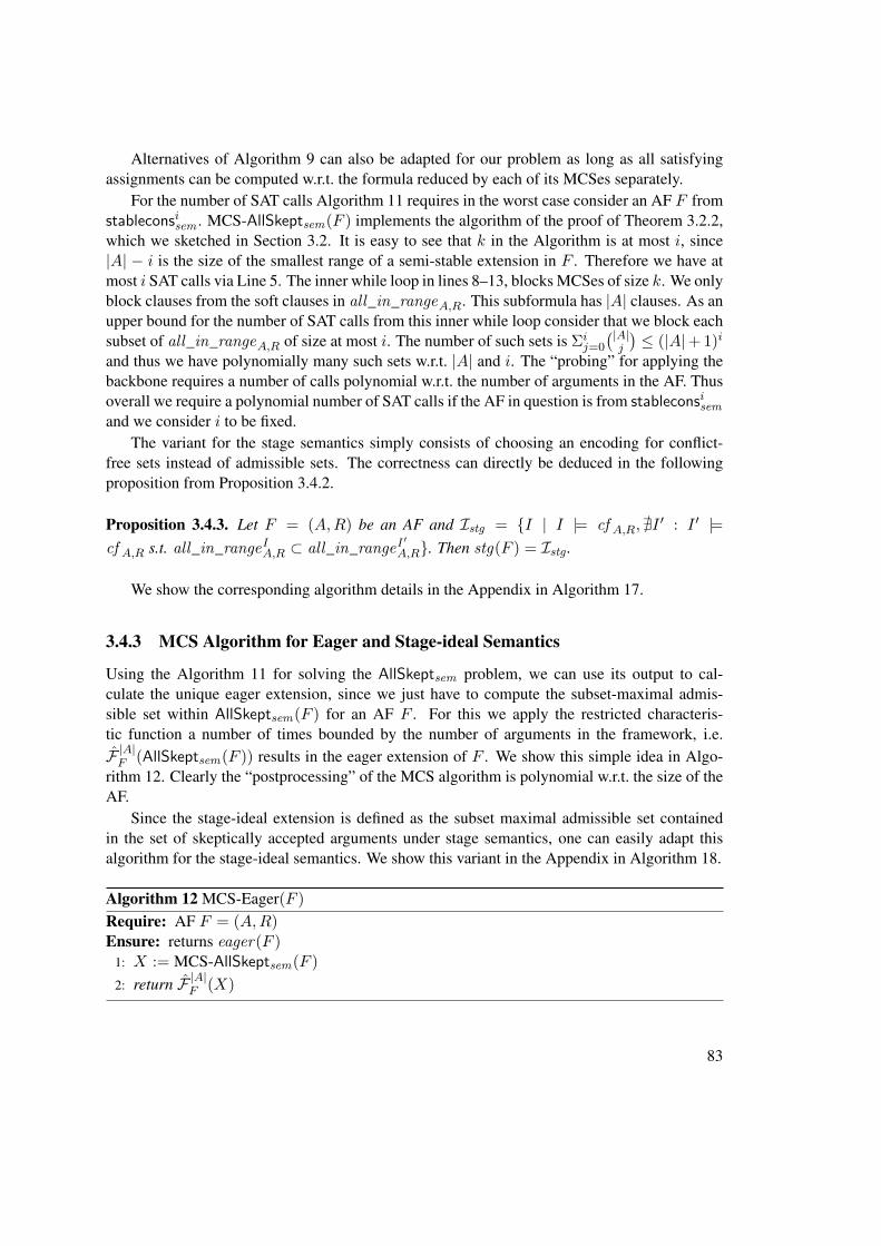
Alternatives of Algorithm 9 can also be adapted for our problem as long as all satisfyingassignments can be computed w.r.t. the formula reduced by each of its MCSes separately.

For the number of SAT calls Algorithm 11 requires in the worst case consider an AF F fromstableconsisem . MCS-AllSkeptsem(F ) implements the algorithm of the proof of Theorem 3.2.2,which we sketched in Section 3.2. It is easy to see that k in the Algorithm is at most i, since|A| − i is the size of the smallest range of a semi-stable extension in F . Therefore we have atmost i SAT calls via Line 5. The inner while loop in lines 8–13, blocks MCSes of size k. We onlyblock clauses from the soft clauses in all_in_rangeA,R. This subformula has |A| clauses. As anupper bound for the number of SAT calls from this inner while loop consider that we block eachsubset of all_in_rangeA,R of size at most i. The number of such sets is Σi

j=0

(|A|j

)≤ (|A|+ 1)i

and thus we have polynomially many such sets w.r.t. |A| and i. The “probing” for applying thebackbone requires a number of calls polynomial w.r.t. the number of arguments in the AF. Thusoverall we require a polynomial number of SAT calls if the AF in question is from stableconsisemand we consider i to be fixed.

The variant for the stage semantics simply consists of choosing an encoding for conflict-free sets instead of admissible sets. The correctness can directly be deduced in the followingproposition from Proposition 3.4.2.

Proposition 3.4.3. Let F = (A,R) be an AF and Istg = {I | I |= cf A,R, @I ′ : I ′ |=cf A,R s.t. all_in_rangeIA,R ⊂ all_in_rangeI

′A,R}. Then stg(F ) = Istg .

We show the corresponding algorithm details in the Appendix in Algorithm 17.

3.4.3 MCS Algorithm for Eager and Stage-ideal Semantics

Using the Algorithm 11 for solving the AllSkeptsem problem, we can use its output to cal-culate the unique eager extension, since we just have to compute the subset-maximal admis-sible set within AllSkeptsem(F ) for an AF F . For this we apply the restricted characteris-tic function a number of times bounded by the number of arguments in the framework, i.e.F |A|F (AllSkeptsem(F )) results in the eager extension of F . We show this simple idea in Algo-rithm 12. Clearly the “postprocessing” of the MCS algorithm is polynomial w.r.t. the size of theAF.

Since the stage-ideal extension is defined as the subset maximal admissible set containedin the set of skeptically accepted arguments under stage semantics, one can easily adapt thisalgorithm for the stage-ideal semantics. We show this variant in the Appendix in Algorithm 18.

Algorithm 12 MCS-Eager(F )

Require: AF F = (A,R)Ensure: returns eager(F )

1: X := MCS-AllSkeptsem(F )

2: return F |A|F (X)

83

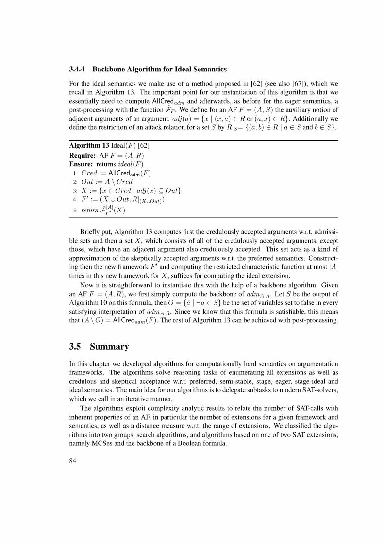
3.4.4 Backbone Algorithm for Ideal Semantics

For the ideal semantics we make use of a method proposed in [62] (see also [67]), which werecall in Algorithm 13. The important point for our instantiation of this algorithm is that weessentially need to compute AllCredadm and afterwards, as before for the eager semantics, apost-processing with the function FF . We define for an AF F = (A,R) the auxiliary notion ofadjacent arguments of an argument: adj(a) = {x | (x, a) ∈ R or (a, x) ∈ R}. Additionally wedefine the restriction of an attack relation for a set S by R|S= {(a, b) ∈ R | a ∈ S and b ∈ S}.

Algorithm 13 Ideal(F ) [62]Require: AF F = (A,R)Ensure: returns ideal(F )

1: Cred := AllCredadm(F )2: Out := A \ Cred3: X := {x ∈ Cred | adj(x) ⊆ Out}4: F ′ := (X ∪Out,R|(X∪Out))5: return F |A|F ′ (X)

Briefly put, Algorithm 13 computes first the credulously accepted arguments w.r.t. admissi-ble sets and then a set X , which consists of all of the credulously accepted arguments, exceptthose, which have an adjacent argument also credulously accepted. This set acts as a kind ofapproximation of the skeptically accepted arguments w.r.t. the preferred semantics. Construct-ing then the new framework F ′ and computing the restricted characteristic function at most |A|times in this new framework for X , suffices for computing the ideal extension.

Now it is straightforward to instantiate this with the help of a backbone algorithm. Givenan AF F = (A,R), we first simply compute the backbone of admA,R. Let S be the output ofAlgorithm 10 on this formula, thenO = {a | ¬a ∈ S} be the set of variables set to false in everysatisfying interpretation of admA,R. Since we know that this formula is satisfiable, this meansthat (A \O) = AllCredadm(F ). The rest of Algorithm 13 can be achieved with post-processing.

3.5 Summary

In this chapter we developed algorithms for computationally hard semantics on argumentationframeworks. The algorithms solve reasoning tasks of enumerating all extensions as well ascredulous and skeptical acceptance w.r.t. preferred, semi-stable, stage, eager, stage-ideal andideal semantics. The main idea for our algorithms is to delegate subtasks to modern SAT-solvers,which we call in an iterative manner.

The algorithms exploit complexity analytic results to relate the number of SAT-calls withinherent properties of an AF, in particular the number of extensions for a given framework andsemantics, as well as a distance measure w.r.t. the range of extensions. We classified the algo-rithms into two groups, search algorithms, and algorithms based on one of two SAT extensions,namely MCSes and the backbone of a Boolean formula.

84

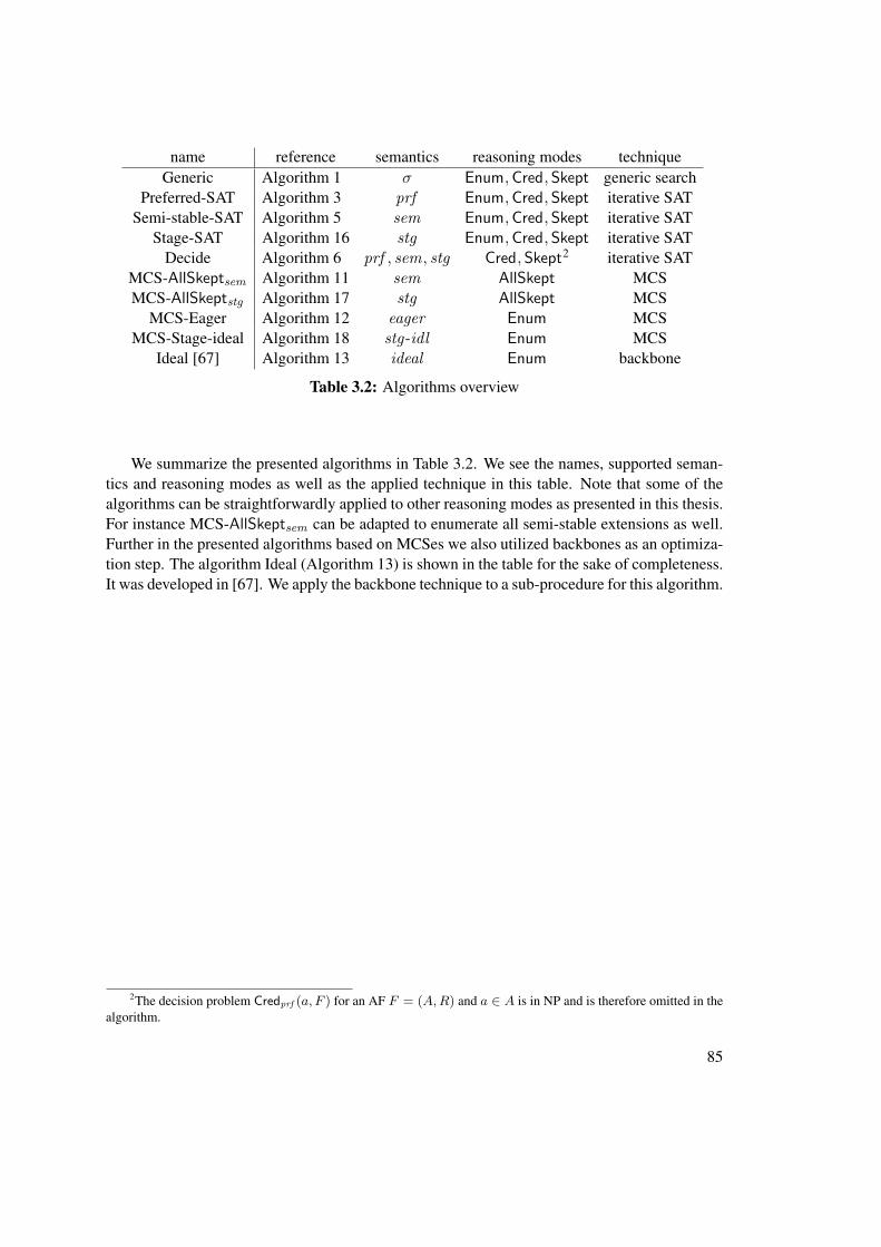
name reference semantics reasoning modes techniqueGeneric Algorithm 1 σ Enum,Cred, Skept generic search

Preferred-SAT Algorithm 3 prf Enum,Cred, Skept iterative SATSemi-stable-SAT Algorithm 5 sem Enum,Cred, Skept iterative SAT

Stage-SAT Algorithm 16 stg Enum,Cred, Skept iterative SATDecide Algorithm 6 prf , sem, stg Cred, Skept2 iterative SAT

MCS-AllSkeptsem Algorithm 11 sem AllSkept MCSMCS-AllSkeptstg Algorithm 17 stg AllSkept MCS

MCS-Eager Algorithm 12 eager Enum MCSMCS-Stage-ideal Algorithm 18 stg-idl Enum MCS

Ideal [67] Algorithm 13 ideal Enum backbone

Table 3.2: Algorithms overview

We summarize the presented algorithms in Table 3.2. We see the names, supported seman-tics and reasoning modes as well as the applied technique in this table. Note that some of thealgorithms can be straightforwardly applied to other reasoning modes as presented in this thesis.For instance MCS-AllSkeptsem can be adapted to enumerate all semi-stable extensions as well.Further in the presented algorithms based on MCSes we also utilized backbones as an optimiza-tion step. The algorithm Ideal (Algorithm 13) is shown in the table for the sake of completeness.It was developed in [67]. We apply the backbone technique to a sub-procedure for this algorithm.

2The decision problem Credprf (a, F ) for an AF F = (A,R) and a ∈ A is in NP and is therefore omitted in thealgorithm.

85

CHAPTER 4Abstract Dialectical Frameworks:

Novel Complexity Results andAlgorithms

This chapter studies the computational properties of abstract dialectical frameworks (ADFs) andshows how to apply the core ideas of the search algorithms from Chapter 3 to ADFs. The maingoal in this chapter is to adapt the generic search Algorithm 1 to problems for the preferredsemantics on ADFs. To this end we require a thorough complexity analysis of the problemson ADFs. In particular the complexity results guide us in two ways. First they show us whichsolvers are suited for the subtasks we delegate to them in the search algorithm. Second, thehardness results indicate, under the standard assumptions of complexity theory, that the tasks weaim to solve are computationally involved problems.

We show that the computational complexity of the considered decision problems of ADFsis one level higher in the polynomial hierarchy compared to the corresponding problems onAFs. Thus, straightforward generalizations of our search algorithms to ADFs have to cope withproblems which are intrinsically harder than it is the case for AFs. In particular this indicatesthat for preferred semantics one requires solvers capable of solving ΣP

2 problems. It turns out,however, that bipolar ADFs (BADFs) are not affected by this complexity jump; the decisionproblems on BADFs have the same computational complexity as their corresponding problemson AFs. Thus we can restrict ourselves to SAT-solvers for solving tasks on BADFs and thepreferred semantics. As a side result of our complexity analysis we obtain a backbone algorithmfor grounded semantics of general ADFs.

We thus present three major contributions in this chapter.

• We prove novel complexity results for decision problems on general ADFs in Section 4.1.1;

• we prove that for bipolar ADFs (BADFs) the complexity is the same as for AFs for thecorresponding decision problems in Section 4.1.2; and

87

• in Section 4.2.1 we show how to generalize the generic search Algorithm 1 for the pre-ferred semantics to ADFs using search engines capable of solving ΣP

2 -complete decisionproblems for general ADFs and using solvers for NP-complete problems for BADFs. Inaddition in Section 4.2.2 we show how to compute the grounded interpretation of an ADFvia a backbone algorithm.

In particular the results for the class of BADFs is of interest, since they incorporate many re-lations between arguments, without increasing the corresponding complexity compared to AFs.Preliminary complexity results w.r.t. the grounded semantics, which we partially use, were de-rived in [34] before work on this thesis has started. Furthermore our results for BADFs canbe seen as a generalization of [34, Proposition 15]. The main results in this chapter are pub-lished in [31, 147].1 A longer version of [147] with detailed proofs is available as a technicalreport [146].

4.1 Complexity Analysis of ADFs

In this section we study the computational complexity of ADFs. We first consider the generalcase in Section 4.1.1 and afterwards BADFs in Section 4.1.2. For a quick reference of the results,the reader is referred to Table 4.5 on page 108.

4.1.1 Complexity Analysis of General ADFs

The complexity of deciding credulous or skeptical acceptance or verifying a solution on ADFsw.r.t. grounded, admissible and preferred semantics is “one level” higher in the polynomial hi-erarchy w.r.t. their counterparts on AFs. For grounded semantics the verification problem isDP-complete for ADFs. We apply proof ideas from [56] to prove hardness of the verificationproblem of preferred semantics and techniques from [63] for the skeptical reasoning problem ofpreferred semantics.

Computational Complexity of the Grounded Semantics

In this section we analyze the complexity of credulous and skeptical reasoning as well as theverification problem for grounded semantics. We begin with a rough upper bound and a straight-forward computation of the grounded interpretation. This somewhat simplistic view is of use togain an intuition of the grounded semantics. Afterwards we show tight upper and lower boundsfor the decision problems. Here we first consider certain properties of three-valued interpre-tations. If a three-valued interpretation I satisfies these properties, then it “approximates” thegrounded interpretation J of an ADF D by J ≤i I , i.e. everything set to true in the grounded in-terpretation is also true in I and every argument set to false in the grounded interpretation is alsofalse in I . Since the properties can essentially be checked by a simple “guess & check” approach,we can derive the corresponding complexity bounds for our decision problems. Subsequently

1We note that the results in [147] are derived using the general framework of approximation fixed point theory(AFT). However the results can be directly adapted for our setting.

88

we use these ideas to encode such an approximation into propositional logic. The benefit of thereduction to propositional logic is that we can use this reduction for implementations.

The grounded interpretation for an ADF D = (S,L,C) can be computed by iterative ap-plications of the characteristic function on the initial interpretation, which sets each argumentin S to u. For convenience we recall the corresponding Definition 2.3.30 from the backgroundchapter.

Definition 2.3.30. LetD = (S,L,C) be an ADF and i ≥ 0 an integer. Define the interpretationgrd i(D) as follows. grd0(D) = I with ∀s ∈ S : I(s) = u. For i > 0 we define grd i(D) =ΓD(grd i−1(D)).

Then by Proposition 2.3.8 it follows that grd |S|(D) is the grounded interpretation for anADF D = (S,L,C), since at each step we either arrive at a fixed point or change the status ofat least one argument.

A useful way of looking at the accepted and rejected arguments w.r.t. the grounded interpre-tation of an ADF D is the following. If an argument s has a tautological acceptance condition,i.e. |= ϕs, then we have to accept it. Otherwise if ϕs is unsatisfiable, then we have to rejectit, i.e. set it to false in the grounded interpretation. This means that any argument set to true inI1 = grd1(D) has a tautological acceptance condition, while the arguments set to false in I1

have an unsatisfiable acceptance condition. Now in the next iteration, we collect all argumentss in It2 for I2 = grd2(D), for which the formula φ = ϕs[I

t1/>][If1/⊥] is valid. If φ is unsat-

isfiable then s ∈ If2 . This can be seen from the fact that in [I1]2 all two-valued interpretationsset all arguments in It1 to true (which have a valid acceptance condition) and all arguments in If1to false (which have an unsatisfiable acceptance condition). Therefore ΓD(I1)(s) = t and thuss ∈ I2 iff φ is valid.

Next follows an easy observation, namely if an argument is undecided in the grounded inter-pretation, then there is a reason for it. This reason can be expressed by two interpretations. Onefor showing that we may not set the argument to true, and one for showing that we may not setit to false in the grounded interpretation. This is captured in the next lemma.

Lemma 4.1.1. Let D = (S,L,C) be an ADF, I its grounded interpretation and u ∈ Iu. Thereexist two two-valued interpretations Iu, Ju ∈ [I]2 such that Iu |= ϕu and Ju 6|= ϕu.

Proof. Assume u ∈ Iu. Suppose now the contrary to the statement in the lemma, i.e. forall two-valued interpretations J ∈ [I]2 we have either that J(ϕu) = t or J(ϕu) = f . Weconsider the first case, since the second one is symmetric. This means that ϕu evaluates totrue for all interpretations in [I]2. Thus ΓD(I)(u) = t. This implies that I 6= ΓD(I), sinceI(u) = u 6= t = ΓD(I)(u). This is a contradiction to I being the grounded interpretation ofD.

We now proceed with a technical lemma, from which we infer the membership part of thecomputational complexity of the reasoning tasks for the grounded semantics.

Definition 4.1.1. Let D = (S,L,C) be an ADF and I a three-valued interpretation on S. Wedefine the following three properties for I w.r.t. D.

89

1. for each a ∈ It there exists a J ∈ [I]2 s.t. J |= ϕa;

2. for each r ∈ If there exists a J ∈ [I]2 s.t. J 6|= ϕr;

3. for each u ∈ Iu there exist J,K ∈ [I]2 s.t. J |= ϕu and K 6|= ϕu.

We denote the set of interpretations which satisfy all three properties w.r.t. D with grd≤i(D).

Now we show that the grounded interpretation satisfies all three properties for any ADF D.On the other hand, if we have a three-valued interpretation J which satisfies the three propertiesfor an ADF D, then grd(D) ≤i J .

Lemma 4.1.2. Let D = (S,L,C) be an ADF and J a three-valued interpretation on S. It holdsthat

• grd(D) ∈ grd≤i(D); and

• if J ∈ grd≤i(D), then grd(D) ≤i J .

Proof. Let I be the grounded interpretation of D, then it is straightforward to show that I ∈grd≤i(D), i.e. it satisfies the three properties of Definition 4.1.1 w.r.t. D. By definition wehave I = ΓD(I) (I is complete in D). Therefore if a ∈ It, then I(a) = t = ΓD(I)(a) andthus K(ϕa) = t for any K ∈ [I]2. For an r ∈ If it is immediate that for any such K wehave K(ϕr) = f . Therefore the first two properties of Definition 4.1.1 are satisfied. Due toLemma 4.1.1 also the third property is satisfied.

We now prove the second item. Assume J ∈ grd≤i(D). We show now by induction onn ≥ 1 that grdn(D) ≤i J . For n = 1 and grd1(D) = K1 we have that if s ∈ Kt

1 then ϕsis a tautology, implying that s ∈ Jt. Suppose the contrary, i.e. s /∈ Jt. Because J satisfiesthe three properties, this implies that there exists a two-valued interpretation which does notsatisfy ϕs. This is a contradiction to ϕs being a tautology. The case for s ∈ Kf

1 is symmetric.Now assume the induction hypothesis Kn = grdn(D) ≤i J and to show that grdn+1(D) ≤i Jholds consider grdn+1(D) = Kn+1. By the hypothesis Kn ≤i J we get that [J ]2 ⊆ [Kn]2. Ifs ∈ (Kt

n+1 \Ktn), then ϕs evaluates to true under any interpretation in [Kn]2. Clearly then there

is no interpretation in [J ]2, which evaluates ϕs to false, therefore s is in Jt, because otherwiseone of the three properties would be violated. Similarly for the arguments set to false. Thisproves the lemma, since grd |S|(D) = I = grd(D).

Note that checking the three properties of Definition 4.1.1 naturally corresponds to guessingtwo-valued interpretations and evaluating a formula. To decide whether a certain argument sis not true in the grounded interpretation of an ADF D, we can simply guess a three-valuedinterpretation I , s.t. I(s) 6= t. We further guess two-valued interpretations from [I]2 to witnessthat I satisfies the three properties. If such a guess succeeds, then due to the preceding lemmait follows that s is not true in the grounded interpretation of D. This line of thought under-lies the following proposition. Recall that for any ADF D = (S,L,C) and s ∈ S we haveCredgrd (s,D) = Skeptgrd (s,D), since the grounded interpretation is unique.

Proposition 4.1.3. Credgrd is coNP-complete for ADFs.

90

Proof. Let D = (S,L,C) be an ADF and s ∈ S. For membership, consider the co-problem,i.e. deciding whether s is not true in the grounded interpretation. Now we guess a three-valuedinterpretation I and a set of two-valued interpretations I ⊆ [I]2 on S with |I| = 2 · |S| ands /∈ It. Clearly we can construct this guess in polynomial time, since we have at most |S| ·2 + 1interpretations over the vocabulary S. Now we check if I ∈ grd≤i(D), i.e. whether it satisfiesthe three properties of Definition 4.1.1 w.r.t. D by considering I as witnesses for each property.If I satisfies the properties w.r.t. D, then J ≤i I with J ∈ grd(D) by Lemma 4.1.2. SinceI(s) 6= t, we have that J(s) 6= t, since otherwise we have J(s) = t 6≤i I(s) if I(s) ∈{f ,u}. This implies that s is not true in the grounded interpretation. Therefore Credgrd (s,D) =Skeptgrd (s,D) = no. Clearly if we cannot guess such an I and successfully check it, thenCredgrd (s,D) = yes.

For hardness, we can adapt the proof of [34, Proposition 13]. We reduce the problem ofVALIDITY to Credgrd (f,D). Let φ be an arbitrary Boolean formula. Then construct D =(atoms(φ) ∪ {f}, L, C) with ϕx = x if x ∈ atoms(φ) and ϕf = φ. The ADF D can beconstructed in polynomial time w.r.t. the size of φ. Clearly if I ∈ grd(D), then for any x ∈atoms(φ) we have I(x) = u. Now assume that Credgrd (f,D) = yes. Then f ∈ It and wehave that for every X with X ⊆ atoms(φ) it holds that X ∪ {f} ∈ [I]2. Since I is admissiblein D, this means that for all such X we have X |= ϕf = φ. Thus φ is valid and a “yes” instanceof VALIDITY. Now assume that φ is valid. Then clearly J with J(x) = u for x ∈ atoms(φ)and J(f) = t is the grounded interpretation of D, by the same reasoning as above.

Using the proof of the preceding proposition, we show the complexity of the verificationproblem.

Theorem 4.1.4. Vergrd is DP-complete for ADFs.

Proof. Let D = (S,L,C) be an ADF and I a three-valued interpretation over S. For member-ship consider the following. For each x ∈ It we can decide whether Credgrd (x,D) = yes witha coNP check. For a y ∈ If we can adapt the proof of Proposition 4.1.3 to show that it is incoNP to decide whether y is false in the grounded interpretation of D. We guess a three-valuedinterpretationK withK(y) 6= f . Further we guess a set of two-valued interpretationsK ⊆ [K]2,which verify that K ∈ grd≤i(D). If this guess is successful, then y is not false in the groundedinterpretation. Thus the problem of deciding whether y is false in the grounded interpretationis in coNP. Therefore we can verify that I ≤i J for J the grounded interpretation of D with|It ∪ If | independent problems in coNP, which can be combined into one problem in coNP.

For verifying that J = I , we also need to verify the undecided arguments in I . We similarlyas before guess a set of two-valued interpretations I ⊆ [I]2 and check whether I ∈ grd≤i(D).If this check is successful, then by Lemma 4.1.2, we know that J ≤i I . The check whetherJ ≤i I holds is in NP. By combining this with the coNP check we have I = J , which solvesthe verification problem. Note that the number and size of the guesses we need to construct foreach argument is polynomial w.r.t. the size of the given ADF D.

For hardness consider the SAT-VALIDITY problem. Let φ and ψ be arbitrary Booleanformulae. W.l.o.g. we assume that atoms(φ) ∩ atoms(ψ) = ∅. We construct an ADF D asfollows. Let D = (atoms(φ) ∪ atoms(ψ) ∪ {d, s, v}, L, C) with

91

• ϕx = x if x ∈ atoms(φ) ∪ atoms(ψ);

• ϕd = d;

• ϕs = φ ∧ d; and

• ϕv = ψ.

The ADF D can be constructed in polynomial time w.r.t. the size of φ and ψ. Then we showthat φ is satisfiable and ψ is valid iff I = grd(D) with I(x) = u for x ∈ atoms(φ)∪atoms(ψ)∪{d, s} and I(v) = t. We can straightforwardly adapt the hardness proof of Proposition 4.1.3 forseeing that if ψ is valid then Credgrd (v,D) = yes and vice versa.

Now assume that φ is satisfiable and ψ is valid. We show that then I is the grounded in-terpretation. For any argument except s it is immediate to see that I assigns the same value asthe grounded interpretation (if the acceptance condition of an argument a is the formula a, thenit is always undecided in the grounded interpretation). What remains to be shown is that s isundecided in the grounded interpretation. Since d is undecided in the grounded interpretationwe have two two-valued interpretations in [grd(D)]2, s.t. one evaluates ϕs to true and another tofalse. Hence I is the grounded interpretation.

Assume otherwise that φ is unsatisfiable or ψ is not valid. In the latter case we haveCredgrd (v,D) = no and thus I is not the grounded interpretation of D. If φ is unsatisfiablethen also ϕs is unsatisfiable and the grounded interpretation sets s to false, unlike the three-valued interpretation I .

Having established the complexity bounds, we are now ready to define the reduction topropositional logic for computing the grounded interpretation of an ADF. We begin with thedefinition of the main part of the Boolean formula we construct.

Definition 4.1.2. Let D = ({s1, ..., sn}, L, C) be an ADF, where we order the arguments and1 ≤ i ≤ n. Then let

grd_formdec(si) = ((s1i ↔ ϕ1

si) ∧ · · · ∧ (s2·ni ↔ ϕ2·n

si ) ∧ ¬sui ) (4.1)

grd_formundec(si) = (ϕisi ∧ ¬ϕi+nsi ∧ sui ) (4.2)

grd_form (D) =∧

1≤j≤n

(grd_formdec(sj) ∨ grd_formundec(sj)

)(4.3)

The propositional formula grd_form (D) is the central part of the reduction for the groundedsemantics for ADFs to Boolean logic. Intuitively grd_formdec(si) consists of 2 · n copies ofan equivalence between the argument si and its acceptance condition. Additionally we requirethat the auxiliary atom sui is false. If this special atom is true in at least one model, then this isinterpreted that si is undecided in the grounded interpretation. The formula grd_formundec(si)is based on the observation from Lemma 4.1.1. In particular for each undecided argument uin the grounded interpretation of an ADF D we have that there is an I ∈ [grd(D)]2 and aninterpretation J ∈ [grd(D)]2, s.t. I(ϕu) = t and J(ϕu) = f . We now state some formalproperties of grd_form (D). First we define a two-valued interpretation Igrd(D).

92

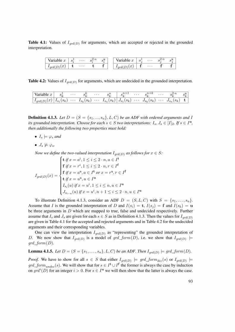
Table 4.1: Values of Igrd(D) for arguments, which are accepted or rejected in the groundedinterpretation.

Variable x s1i · · · s2·n

i suiIgrd(D)(x) t · · · t f

Variable x s1j · · · s2·n

j sujIgrd(D)(x) f · · · f f

Table 4.2: Values of Igrd(D) for arguments, which are undecided in the grounded interpretation.

Variable x s1k · · · skk · · · snk sn+1

k · · · sn+kk · · · s2·n

k sukIgrd(D)(x) Is1(sk) · · · Isk(sk) · · · Isn(sk) Js1(sk) · · · Jsk(sk) · · · Jsn(sk) t

Definition 4.1.3. Let D = (S = {s1, ..., sn}, L, C) be an ADF with ordered arguments and Iits grounded interpretation. Choose for each s ∈ S two interpretations: Is, Js ∈ [I]2. If s ∈ Iu,then additionally the following two properties must hold:

• Is |= ϕs and

• Js 6|= ϕs.

Now we define the two-valued interpretation Igrd(D) as follows for x ∈ S:

Igrd(D)(x) =

t if x = ai, 1 ≤ i ≤ 2 · n, a ∈ Itf if x = ri, 1 ≤ i ≤ 2 · n, r ∈ Iff if x = au, a ∈ It or x = ru, r ∈ Ift if x = uu, u ∈ IuIsi(u) if x = ui, 1 ≤ i ≤ n, u ∈ IuJsi−n(u) if x = ui, n+ 1 ≤ i ≤ 2 · n, u ∈ Iu

To illustrate Definition 4.1.3, consider an ADF D = (S,L,C) with S = {s1, . . . , sn}.Assume that I is the grounded interpretation of D and I(si) = t, I(sj) = f and I(sk) = ube three arguments in D which are mapped to true, false and undecided respectively. Furtherassume that Is and Js are given for each s ∈ S as in Definition 4.1.3. Then the values for Igrd(D)

are given in Table 4.1 for the accepted and rejected arguments and in Table 4.2 for the undecidedarguments and their corresponding variables.

One can view the interpretation Igrd(D) as “representing” the grounded interpretation ofD. We now show that Igrd(D) is a model of grd_form (D), i.e. we show that Igrd(D) |=grd_form (D).

Lemma 4.1.5. Let D = (S = {s1, . . . , sn}, L, C) be an ADF. Then Igrd(D) |= grd_form (D).

Proof. We have to show for all s ∈ S that either Igrd(D) |= grd_formdec(s) or Igrd(D) |=grd_formundec(s). We will show that for s ∈ It ∪ If the former is always the case by inductionon grd i(D) for an integer i > 0. For s ∈ Iu we will then show that the latter is always the case.

93

• Induction base (i = 1): Let grd1(D) = J , then Igrd(D) |= grd_formdec(s) for s ∈Jt ∪ J f . First consider the case that s ∈ Jt, then ϕs is tautological and Igrd(D)(s

j) = tfor 1 ≤ j ≤ 2 · n. This means that all equivalences of grd_formdec(s) are satisfied, andsince Igrd(D)(s

u) = f we know that this subformula is satisfied by Igrd(D). Similarly fors ∈ J f .

• Induction hypothesis: For an integer i, let grd i(D) = J , then Igrd(D) |= grd_formdec(s)

for s ∈ Jt ∪ J f .

• Induction step: Assume that the induction hypothesis is true and grd i(D) = J . Letgrd i+1(D) = K. For every s ∈ Kt, the formula ϕs is tautological if the variables fromJt are set to true and J f are set to false in ϕs, i.e. |= ϕs[J

t/>][J f/⊥]. If this would not bethe case, then s 6∈ Kt. Hence all equivalences of grd_formdec(s) are satisfied, and againsince Igrd(D)(s

u) = f we know that Igrd(D) |= grd_formdec(s). Similarly for s ∈ Kf .

For si ∈ Iu we show that Igrd(D) |= grd_formundec(si). By construction we know thatIgrd(D) |= ϕisi and Igrd(D) 6|= ϕn+i

si . Further we have that Igrd(D)(sui ) = t, hence Igrd(D) |=

grd_formundec(si) for all si ∈ Iu.

Next we show that grd_form (D) entails certain atoms, corresponding to accepted and re-jected arguments in the ADF w.r.t. grounded semantics.

Lemma 4.1.6. Let D = (S,L,C) be an ADF, I its grounded interpretation and |S| = n. Thengrd_form (D) |= ∧a∈It(a

1 ∧ · · · ∧ a2n ∧ ¬au) ∧∧r∈If (¬r1 ∧ · · · ∧ ¬r2n ∧ ¬ru).

Proof. LetX ⊆ S be a set of arguments, then we define the following helper functionsA(X) =∧x∈X(x1 ∧ · · · ∧ x2·n ∧ ¬xu) and R(X) =

∧x∈X(¬x1 ∧ · · · ∧ ¬x2·n ∧ ¬xu). We now prove

by induction on grd i(D) the lemma. Note that grd_form (D) is satisfiable by Lemma 4.1.5.

• Induction base (i = 1): Let grd1(D) = J , then the entailment grd_form (D) |= A(Jt) ∧R(J f ) follows, since ϕa ≡ > and ϕr ≡ ⊥ for a ∈ Jt and r ∈ J f . Consider the case thats ∈ Jt, then ¬ϕs is unsatisfiable, hence grd_formundec(s) is unsatisfiable. Therefore,since at least one model of grd_form exists, we know that in all models of it we have tosatisfy A(Jt). The proof for R(J f ) is analogous.

• Induction hypothesis: For an integer i, let grd i(D) = J , then grd_form (D) |= A(Jt) ∧R(J f ).

• Induction step: Assume that the induction hypothesis is true. Let grd i(D) = J andgrd i+1(D) = K. If grd_form (D) |= A(Jt)∧R(J f ), then in all models of grd_form (D)(which exist, due to Lemma 4.1.5) we have that the renamed atoms of a ∈ Jt are set totrue and r ∈ J f are set to false, i.e. J(aj) = t and J(rj) = f for 1 ≤ j ≤ 2 · n.Hence ϕb[Jt/>][J f/⊥] is tautological for b ∈ Kt, i.e. cannot be falsified anymore andϕc[J

t/>][J f/⊥] for c ∈ Kf cannot evaluate to true. This means that both subformu-lae grd_formundec(b) and grd_formundec(c) are unsatisfiable. In all models satisfyinggrd_formdec(b) we have that b1 ∧ · · · ∧ b2·n ∧ ¬bu is entailed. Similarly for c.

94

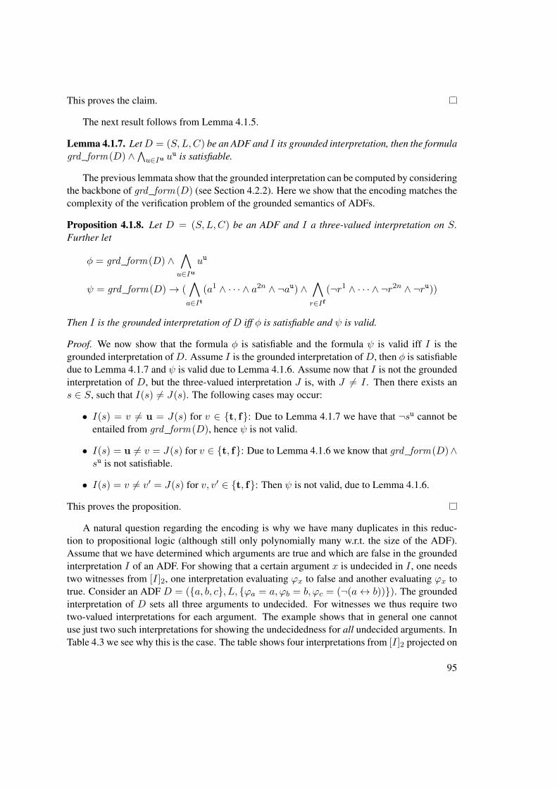
This proves the claim.

The next result follows from Lemma 4.1.5.

Lemma 4.1.7. LetD = (S,L,C) be an ADF and I its grounded interpretation, then the formulagrd_form (D) ∧∧u∈Iu u

u is satisfiable.

The previous lemmata show that the grounded interpretation can be computed by consideringthe backbone of grd_form (D) (see Section 4.2.2). Here we show that the encoding matches thecomplexity of the verification problem of the grounded semantics of ADFs.

Proposition 4.1.8. Let D = (S,L,C) be an ADF and I a three-valued interpretation on S.Further let

φ = grd_form (D) ∧∧u∈Iu

uu

ψ = grd_form (D)→ (∧a∈It

(a1 ∧ · · · ∧ a2n ∧ ¬au) ∧∧r∈If

(¬r1 ∧ · · · ∧ ¬r2n ∧ ¬ru))

Then I is the grounded interpretation of D iff φ is satisfiable and ψ is valid.

Proof. We now show that the formula φ is satisfiable and the formula ψ is valid iff I is thegrounded interpretation ofD. Assume I is the grounded interpretation ofD, then φ is satisfiabledue to Lemma 4.1.7 and ψ is valid due to Lemma 4.1.6. Assume now that I is not the groundedinterpretation of D, but the three-valued interpretation J is, with J 6= I . Then there exists ans ∈ S, such that I(s) 6= J(s). The following cases may occur:

• I(s) = v 6= u = J(s) for v ∈ {t, f}: Due to Lemma 4.1.7 we have that ¬su cannot beentailed from grd_form (D), hence ψ is not valid.

• I(s) = u 6= v = J(s) for v ∈ {t, f}: Due to Lemma 4.1.6 we know that grd_form (D)∧su is not satisfiable.

• I(s) = v 6= v′ = J(s) for v, v′ ∈ {t, f}: Then ψ is not valid, due to Lemma 4.1.6.

This proves the proposition.

A natural question regarding the encoding is why we have many duplicates in this reduc-tion to propositional logic (although still only polynomially many w.r.t. the size of the ADF).Assume that we have determined which arguments are true and which are false in the groundedinterpretation I of an ADF. For showing that a certain argument x is undecided in I , one needstwo witnesses from [I]2, one interpretation evaluating ϕx to false and another evaluating ϕx totrue. Consider an ADF D = ({a, b, c}, L, {ϕa = a, ϕb = b, ϕc = (¬(a↔ b))}). The groundedinterpretation of D sets all three arguments to undecided. For witnesses we thus require twotwo-valued interpretations for each argument. The example shows that in general one cannotuse just two such interpretations for showing the undecidedness for all undecided arguments. InTable 4.3 we see why this is the case. The table shows four interpretations from [I]2 projected on

95

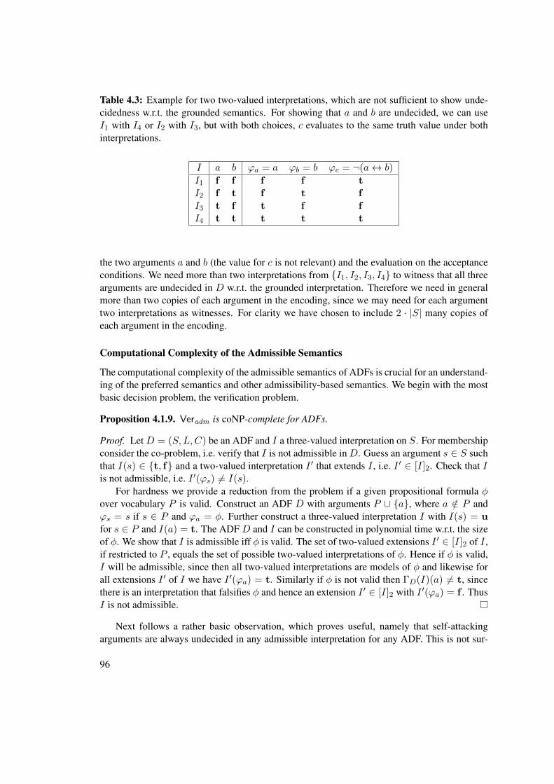
Table 4.3: Example for two two-valued interpretations, which are not sufficient to show unde-cidedness w.r.t. the grounded semantics. For showing that a and b are undecided, we can useI1 with I4 or I2 with I3, but with both choices, c evaluates to the same truth value under bothinterpretations.

I a b ϕa = a ϕb = b ϕc = ¬(a↔ b)

I1 f f f f tI2 f t f t fI3 t f t f fI4 t t t t t

the two arguments a and b (the value for c is not relevant) and the evaluation on the acceptanceconditions. We need more than two interpretations from {I1, I2, I3, I4} to witness that all threearguments are undecided in D w.r.t. the grounded interpretation. Therefore we need in generalmore than two copies of each argument in the encoding, since we may need for each argumenttwo interpretations as witnesses. For clarity we have chosen to include 2 · |S| many copies ofeach argument in the encoding.

Computational Complexity of the Admissible Semantics

The computational complexity of the admissible semantics of ADFs is crucial for an understand-ing of the preferred semantics and other admissibility-based semantics. We begin with the mostbasic decision problem, the verification problem.

Proposition 4.1.9. Veradm is coNP-complete for ADFs.

Proof. Let D = (S,L,C) be an ADF and I a three-valued interpretation on S. For membershipconsider the co-problem, i.e. verify that I is not admissible inD. Guess an argument s ∈ S suchthat I(s) ∈ {t, f} and a two-valued interpretation I ′ that extends I , i.e. I ′ ∈ [I]2. Check that Iis not admissible, i.e. I ′(ϕs) 6= I(s).

For hardness we provide a reduction from the problem if a given propositional formula φover vocabulary P is valid. Construct an ADF D with arguments P ∪ {a}, where a /∈ P andϕs = s if s ∈ P and ϕa = φ. Further construct a three-valued interpretation I with I(s) = ufor s ∈ P and I(a) = t. The ADF D and I can be constructed in polynomial time w.r.t. the sizeof φ. We show that I is admissible iff φ is valid. The set of two-valued extensions I ′ ∈ [I]2 of I ,if restricted to P , equals the set of possible two-valued interpretations of φ. Hence if φ is valid,I will be admissible, since then all two-valued interpretations are models of φ and likewise forall extensions I ′ of I we have I ′(ϕa) = t. Similarly if φ is not valid then ΓD(I)(a) 6= t, sincethere is an interpretation that falsifies φ and hence an extension I ′ ∈ [I]2 with I ′(ϕa) = f . ThusI is not admissible.

Next follows a rather basic observation, which proves useful, namely that self-attackingarguments are always undecided in any admissible interpretation for any ADF. This is not sur-

96

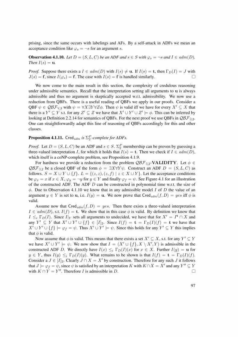
prising, since the same occurs with labelings and AFs. By a self-attack in ADFs we mean anacceptance condition like ϕs = ¬s for an argument s.

Observation 4.1.10. Let D = (S,L,C) be an ADF and s ∈ S with ϕs = ¬s and I ∈ adm(D).Then I(s) = u.

Proof. Suppose there exists a I ∈ adm(D) with I(s) 6= u. If I(s) = t, then ΓD(I) = J withJ(s) = f , since I(ϕs) = f . The case with I(s) = f is handled similarly.

We now come to the main result in this section, the complexity of credulous reasoningunder admissible semantics. Recall that the interpretation setting all arguments to u is alwaysadmissible and thus no argument is skeptically accepted w.r.t. admissibility. We now use areduction from QBFs. There is a useful reading of QBFs we apply in our proofs. Consider aQBF ψ ∈ QBF∀,3 with ψ = ∀X∃Y ∀Zφ. Then ψ is valid iff we have for every X ′ ⊆ X thatthere is a Y ′ ⊆ Y s.t. for any Z ′ ⊆ Z we have that X ′ ∪ Y ′ ∪ Z ′ |= φ. This can be inferred bylooking at Definition 2.2.14 for semantics of QBFs. For the next proof we use QBFs inQBF∃,2.One can straightforwardly adapt this line of reasoning of QBFs accordingly for this and otherclasses.

Proposition 4.1.11. Credadm is ΣP2 -complete for ADFs.

Proof. Let D = (S,L,C) be an ADF and s ∈ S. ΣP2 membership can be proven by guessing a

three-valued interpretation I , for which it holds that I(s) = t. Then we check if I ∈ adm(D),which itself is a coNP-complete problem, see Proposition 4.1.9.

For hardness we provide a reduction from the problem QBF∃,2-VALIDITY. Let φ ∈QBF∃,2 be a closed QBF of the form φ = ∃X∀Y ψ. Construct an ADF D = (S,L,C) asfollows. S = X ∪ Y ∪ {f}. L = {(z, z), (z, f) | z ∈ X ∪ Y }. Let the acceptance conditionsbe ϕx = x if x ∈ X , ϕy = ¬y for y ∈ Y and finally ϕf = ψ. See Figure 4.1 for an illustrationof the constructed ADF. The ADF D can be constructed in polynomial time w.r.t. the size ofφ. Due to Observation 4.1.10 we know that in any admissible model I of D the value of anargument y ∈ Y is set to u, i.e. I(y) = u. We now prove that Credadm(f,D) = yes iff φ isvalid.

Assume now that Credadm(f,D) = yes. Then there exists a three-valued interpretationI ∈ adm(D), s.t. I(f) = t. We show that in this case φ is valid. By definition we know thatI ≤i ΓD(I). Since I|Y sets all arguments to undecided, we have that for X ′ = It ∩ X andany Y ′ ⊆ Y that X ′ ∪ Y ′ ∪ {f} ∈ [I]2. Since I(f) = t = ΓD(I)(f) = t we have thatX ′ ∪ Y ′ ∪ {f} |= ϕf = ψ. Thus X ′ ∪ Y ′ |= ψ. Since this holds for any Y ′ ⊆ Y this impliesthat φ is valid.

Now assume that φ is valid. This means that there exists a set X ′ ⊆ X , s.t. for any Y ′ ⊆ Ywe have X ′ ∪ Y ′ |= ψ. We now show that I = (X ′ ∪ {f}, X \ X ′, Y ) is admissible in theconstructed ADF D. We directly have I(x) ≤i ΓD(I)(x) for x ∈ X . Further I(y) = u fory ∈ Y , thus I(y) ≤i ΓD(I)(y). What remains to be shown is that I(f) = t = ΓD(I)(f).Consider a J ∈ [I]2. Clearly J ∩X = X ′ by construction. Therefore for any such J it followsthat J |= ϕf = ψ, since ψ is satisfied by an interpretationK withK∩X = X ′ and any Y ′′ ⊆ Ywith K ∩ Y = Y ′′. Therefore I is admissible in D.

97

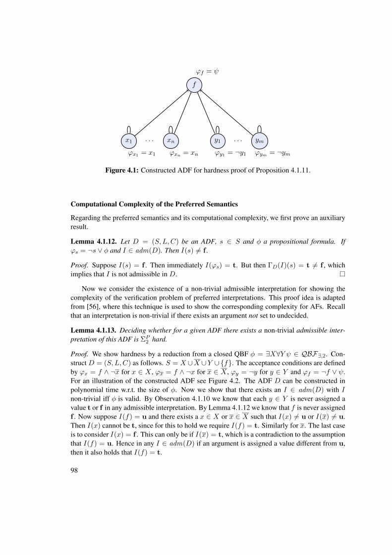
f

ϕf = ψ

x1

ϕx1 = x1

· · · xn

ϕxn = xn

y1

ϕy1 = ¬y1

· · · ym

ϕym = ¬ym

Figure 4.1: Constructed ADF for hardness proof of Proposition 4.1.11.

Computational Complexity of the Preferred Semantics

Regarding the preferred semantics and its computational complexity, we first prove an auxiliaryresult.

Lemma 4.1.12. Let D = (S,L,C) be an ADF, s ∈ S and φ a propositional formula. Ifϕs = ¬s ∨ φ and I ∈ adm(D). Then I(s) 6= f .

Proof. Suppose I(s) = f . Then immediately I(ϕs) = t. But then ΓD(I)(s) = t 6= f , whichimplies that I is not admissible in D.

Now we consider the existence of a non-trivial admissible interpretation for showing thecomplexity of the verification problem of preferred interpretations. This proof idea is adaptedfrom [56], where this technique is used to show the corresponding complexity for AFs. Recallthat an interpretation is non-trivial if there exists an argument not set to undecided.

Lemma 4.1.13. Deciding whether for a given ADF there exists a non-trivial admissible inter-pretation of this ADF is ΣP

2 hard.

Proof. We show hardness by a reduction from a closed QBF φ = ∃X∀Y ψ ∈ QBF∃,2. Con-struct D = (S,L,C) as follows. S = X ∪X ∪Y ∪{f}. The acceptance conditions are definedby ϕx = f ∧ ¬x for x ∈ X , ϕx = f ∧ ¬x for x ∈ X , ϕy = ¬y for y ∈ Y and ϕf = ¬f ∨ ψ.For an illustration of the constructed ADF see Figure 4.2. The ADF D can be constructed inpolynomial time w.r.t. the size of φ. Now we show that there exists an I ∈ adm(D) with Inon-trivial iff φ is valid. By Observation 4.1.10 we know that each y ∈ Y is never assigned avalue t or f in any admissible interpretation. By Lemma 4.1.12 we know that f is never assignedf . Now suppose I(f) = u and there exists a x ∈ X or x ∈ X such that I(x) 6= u or I(x) 6= u.Then I(x) cannot be t, since for this to hold we require I(f) = t. Similarly for x. The last caseis to consider I(x) = f . This can only be if I(x) = t, which is a contradiction to the assumptionthat I(f) = u. Hence in any I ∈ adm(D) if an argument is assigned a value different from u,then it also holds that I(f) = t.

98

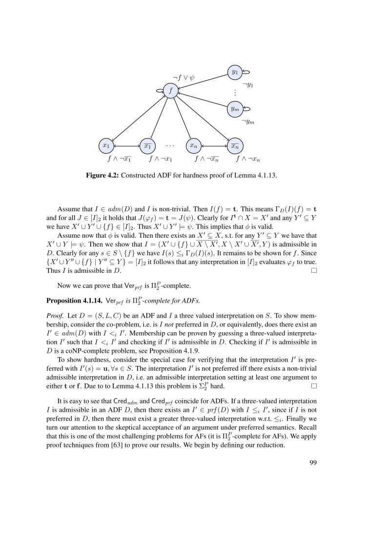
f

¬f ∨ ψ

x1

f ∧ ¬x1

x1

f ∧ ¬x1

· · · xn

f ∧ ¬xn

xn

f ∧ ¬xn

y1

¬y1...

ym

¬ym

Figure 4.2: Constructed ADF for hardness proof of Lemma 4.1.13.

Assume that I ∈ adm(D) and I is non-trivial. Then I(f) = t. This means ΓD(I)(f) = tand for all J ∈ [I]2 it holds that J(ϕf ) = t = J(ψ). Clearly for It ∩X = X ′ and any Y ′ ⊆ Ywe have X ′ ∪ Y ′ ∪ {f} ∈ [I]2. Thus X ′ ∪ Y ′ |= ψ. This implies that φ is valid.

Assume now that φ is valid. Then there exists an X ′ ⊆ X , s.t. for any Y ′ ⊆ Y we have thatX ′ ∪ Y |= ψ. Then we show that I = (X ′ ∪ {f} ∪X \X ′, X \X ′ ∪X ′, Y ) is admissible inD. Clearly for any s ∈ S \ {f} we have I(s) ≤i ΓD(I)(s). It remains to be shown for f . Since{X ′ ∪Y ′′ ∪{f} | Y ′′ ⊆ Y } = [I]2 it follows that any interpretation in [I]2 evaluates ϕf to true.Thus I is admissible in D.

Now we can prove that Verprf is ΠP2 -complete.

Proposition 4.1.14. Verprf is ΠP2 -complete for ADFs.

Proof. Let D = (S,L,C) be an ADF and I a three valued interpretation on S. To show mem-bership, consider the co-problem, i.e. is I not preferred in D, or equivalently, does there exist anI ′ ∈ adm(D) with I <i I ′. Membership can be proven by guessing a three-valued interpreta-tion I ′ such that I <i I ′ and checking if I ′ is admissible in D. Checking if I ′ is admissible inD is a coNP-complete problem, see Proposition 4.1.9.

To show hardness, consider the special case for verifying that the interpretation I ′ is pre-ferred with I ′(s) = u, ∀s ∈ S. The interpretation I ′ is not preferred iff there exists a non-trivialadmissible interpretation in D, i.e. an admissible interpretation setting at least one argument toeither t or f . Due to to Lemma 4.1.13 this problem is ΣP

2 hard.

It is easy to see that Credadm and Credprf coincide for ADFs. If a three-valued interpretationI is admissible in an ADF D, then there exists an I ′ ∈ prf (D) with I ≤i I ′, since if I is notpreferred in D, then there must exist a greater three-valued interpretation w.r.t. ≤i. Finally weturn our attention to the skeptical acceptance of an argument under preferred semantics. Recallthat this is one of the most challenging problems for AFs (it is ΠP

2 -complete for AFs). We applyproof techniques from [63] to prove our results. We begin by defining our reduction.

99

f

¬f ∨ ψx1

x1...

xn

xn

y1

f ∧ ¬y1

y1

f ∧ ¬y1

· · · ym

f ∧ ¬ym

ym

f ∧ ¬ym

z1

¬z1...

zo

¬zo

Figure 4.3: Constructed ADF for hardness proof of Theorem 4.1.17.

Definition 4.1.4. Let φ ∈ QBF∀,3 be a closed QBF, with the form φ = ∀X∃Y ∀Zψ. We definethe ADF Dprf (φ) = (S,L,C) with S = X ∪ Y ∪ Y ∪ Z ∪ {f} and the acceptance conditionsas follows.

• ϕx = x if x ∈ X ,

• ϕy = ¬y ∧ f if y ∈ Y ,

• ϕy = ¬y ∧ f if y ∈ Y ,

• ϕz = ¬z if z ∈ Z,

• ϕf = ¬f ∨ ψ.

As usual the links L are defined implicitly via C.

See Figure 4.3 for an illustration of the constructed ADF from Definition 4.1.4. The ADFDprf (φ) can be constructed in polynomial time w.r.t. the size of φ. We now prove some propertiesof this ADF. First we show that for any two-valued truth assignment on the arguments inX thereis at least one preferred interpretation setting the arguments in X to these values.

Lemma 4.1.15. Let φ = ∀X∃Y ∀Zψ be a closed QBF, Dprf (φ) = (S,L,C), the set of alltwo-valued interpretations on X be J = {J | x ∈ X, J(x) = t or J(x) = f} and the set ofpreferred models of Dprf (φ) restricted to X be I = {I|X | I ∈ prf (Dprf (φ))}. It then holdsthat J = I.

Proof. Assume J ∈ J , we need to show that then there exists an I ∈ prf (Dprf (φ)) withJ = I|X . Consider J ′ with J ′|X= J and J ′(s) = u for s ∈ S \X . Clearly J ′ is admissible inDprf (φ). Now we have that there exists an I ∈ prf (Dprf (φ)) s.t. J ′ ≤i I .

Now assume that I ∈ prf (Dprf (φ)). We need to show that then there exists a J ∈ J suchthat I|X = J . Suppose there exists an x ∈ X such that I(x) = u. This is a contradiction to I

100

being preferred in prf (Dprf (φ)), since we can consider an I ′ for which it holds that I ′(s) = I(s)for s ∈ S \ {x}, but I ′(x) 6= u. Then I ′ is also admissible, which contradicts that I is preferred.This means that I(x) 6= u for any x ∈ X . Since J contains any possible two-valued truth valuecombination of the variables in X , we can find a matching J ∈ J such that the claim holds.

Next we show that an admissible interpretation setting all arguments except the ones in Znot to undecided is a preferred interpretation of Dprf (φ) and in this case there is no preferredinterpretation which sets to X the same values, but leaves the others (those in S \X) undecided.

Lemma 4.1.16. Let φ = ∀X∃Y ∀Zψ be a closed QBF,Dprf (φ) = (S,L,C), I ∈ adm(Dprf (φ)).If I assigns a truth value different from u to variables in X ∪ Y ∪ Y and I(f) = t, then thefollowing two statements hold.

• I ∈ prf (Dprf (φ)); and

• @J ∈ prf (Dprf (φ)) such that J |X = I|X and I(s) = u for s ∈ (S \X)

Proof. Assume I ∈ adm(Dprf (φ)) and I(s) 6= u for s ∈ S \ Z and I(f) = t. Due toObservation 4.1.10 it holds that any admissible model sets the variables in Z to undecided, andI is admissible, that is there cannot be an I ′ with I <i I ′ such that I ′ is admissible in Dprf (φ).Hence I is preferred in Dprf (φ).

Now suppose that J ∈ prf (Dprf (φ)) and J(s) = u for s ∈ S \X and J |X = I|X . ClearlyJ <i I , hence J cannot be preferred.

Finally we are able to prove that Skeptprf is ΠP3 -complete for ADFs.

Theorem 4.1.17. Skeptprf is ΠP3 -complete for ADFs.

Proof. LetD = (S,L,C) be an ADF and s ∈ S. To show membership consider the co-problem,i.e. deciding whether there exists a preferred interpretation I ′ of D, which does not set s to t.Checking if I ′ is preferred in D is a ΠP

2 -complete problem, see Proposition 4.1.14.For hardness consider a reduction from a closed QBF φ = ∀X∃Y ∀Zψ, then construct

Dprf (φ) as in Definition 4.1.4. First we use previous lemmata to show some properties of theconstructed ADF. By Lemma 4.1.15 we can infer that for any X ′ ⊆ X there is a set of preferredinterpretations, setting X ′ to true and X \X ′ to false. Also due to Lemma 4.1.15, we know thatany preferred interpretation is captured this way, i.e. there is no preferred interpretation settingone x ∈ X to undecided. Further in any admissible interpretation we have that any y ∈ Y isset to undecided, due to Observation 4.1.10. Further as shown in Lemma 4.1.12 we know thatI(f) 6= f for any I ∈ adm(Dprf (φ)). We now prove that Skeptprf (f,D) = yes iff φ is valid.

Assume that φ is valid. Now consider an arbitrary X ′ ⊆ X . Since φ is valid, we knowthat there is a Y ′ ⊆ Y s.t. for any Z ′ ⊆ Z we have X ′ ∪ Y ′ ∪ Z ′ |= ψ. Let the three-valuedinterpretation I be defined as

• It = X ′ ∪ Y ′ ∪ (Y \ Y ′) ∪ {f};

• If = (X \X ′) ∪ (Y \ Y ′) ∪ Y ′; and

101

• Iu = Z.

We now show that I is preferred inDprf (φ). We can directly infer that I(s) ≤i ΓDprf (φ)(I)(s)

for s ∈ X ∪ Y ∪ Z. It remains to show that I(f) ≤i ΓDprf (φ)(I)(f) to see that I is admissible.

Since [I]2 = {X ′ ∪ Y ′ ∪ Z ′ ∪ (Y \ Y ′) ∪ {f} | Z ′ ⊆ Z} we know that any two-valuedinterpretation in [I]2 is a model of ψ and thus also a model of ϕf . Therefore I is admissible inDprf (φ). Clearly I is also preferred since only arguments in Z are undecided.

Now we show that all admissible interpretations which assign to the arguments inX the samevalue as I either also set f to true or are not preferred. Suppose that there is a J ∈ adm(D)with J |X = I and J(f) 6= t. Similarly as in the proof of Lemma 4.1.13 we know that f isnever assigned the value false in an admissible interpretation and the arguments in Y and Y areassigned a value different from undecided only if f is assigned true. This means that J sets allarguments except the ones fromX to undecided. Clearly then J ≤i I and J cannot be preferred.Thus for an arbitraryX ′ ⊆ X all preferred interpretationsK ∈ prf (Dprf (φ)) withKt∩X = X ′

also have the property that K(f) = t. Since φ is valid by assumption, we infer that for any suchX ′ we can find corresponding values of Y ′ and have a preferred interpretation setting f to trueand no preferred interpretation setting it otherwise. Therefore f is skeptically accepted.

Now we prove the other direction of the correctness of the reduction, i.e. assume thatSkeptprf (f,D) = yes. We have to show that then φ is valid. Due to Lemma 4.1.15, wehave all combinations for setting the truth values for variables in X in the preferred interpreta-tions. Furthermore, since for each of them the value of f is set to true, the values for Y ∪ Ymust be set to true or false and cannot be undecided. Therefore, again consider an arbitraryX ′ ⊆ X . There is at least one I ∈ prf (Dprf (φ)) s.t. It ∩ X = X ′. Further let Y ′ = It ∩ Y .Now we have X ′ ∪ Y ′ ∪ (Y \ Y ′) ∪ Z ′ ∪ {f} ∈ [I]2 for any Z ′ ⊆ Z, since Iu = Z. SinceI(f) ≤i ΓDprf (φ)

(I)(f) we know that X ′ ∪ Y ′ ∪ Z ′ ∪ {f} |= ϕf and thus X ′ ∪ Y ′ ∪ Z ′ |= ψ.Since this holds for any X ′ ⊆ X this implies that φ is valid.

4.1.2 Complexity Analysis of Bipolar ADFs

Brewka and Woltran [34, Proposition 15] already showed that the verification problem of thegrounded semantics is tractable if the ADF is a bipolar ADF with known links. We can signifi-cantly extend their observation to admissible and preferred semantics and show that BADFs withknown link types have the same computational complexity as AFs. We note that some of the fol-lowing ideas are already present in the proof of [34, Proposition 15]. Consider the characteristicfunction ΓD for an ADF D. If D is a general ADF, then we basically have to consider for thecomputation of ΓD(I) for a three-valued interpretation I all two-valued interpretations from [I]2and evaluate them on the acceptance conditions. For BADFs it suffices to consider per arguments in the BADF just one interpretation in [I]2 to decide whether I(s) ≤i ΓD(I)(s). We call thisinterpretation canonical and provide a function canonD : 2S→{t,f ,u} × S × {t, f} → 2S→{t,f}.This function takes a three-valued interpretation, an argument and a truth value as input. It re-sults in a two-valued interpretation. The idea is that for an BADF D = (S,L = L+ ∪ L−, C)and a three-valued interpretation I on S, an argument s ∈ S we have canonD(I, s, t) = Jand J(ϕs) = t iff ΓD(I)(s) = t. For computing the result ΓD(I)(s) we then need two suchcanonical interpretations. One for each of the two truth values t and f .

102

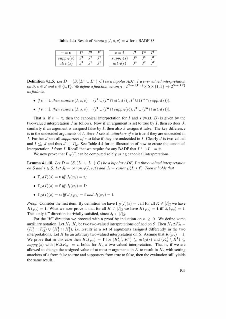
Table 4.4: Result of canonD(I, s, v) = J for a BADF D

v = t It Iu If

suppD(s) Jt J f J f

attD(s) Jt Jt J f

v = f It Iu If

suppD(s) Jt Jt J f

attD(s) Jt J f J f

Definition 4.1.5. Let D = (S, (L+ ∪ L−), C) be a bipolar ADF, I a two-valued interpretationon S, s ∈ S and v ∈ {t, f}. We define a function canonD : 2S→{t,f ,u}×S×{t, f} → 2S→{t,f}

as follows.

• if v = t, then canonD(I, s, v) = (It ∪ (Iu ∩ attD(s)), If ∪ (Iu ∩ suppD(s)));

• if v = f , then canonD(I, s, v) = (It ∪ (Iu ∩ suppD(s)), If ∪ (Iu ∩ attD(s))).

That is, if v = t, then the canonical interpretation for I and s (w.r.t. D) is given by thetwo-valued interpretation J as follows. Now if an argument is set to true by I , then so does J ,similarly if an argument is assigned false by I , then also J assigns it false. The key differenceis in the undecided arguments of I . Here J sets all attackers of s to true if they are undecided inI . Further J sets all supporters of s to false if they are undecided in I . Clearly J is two-valuedand I ≤i J and thus J ∈ [I]2. See Table 4.4 for an illustration of how to create the canonicalinterpretation J from I . Recall that we require for any BADF that L+ ∩ L− = ∅.

We now prove that ΓD(I) can be computed solely using canonical interpretations.

Lemma 4.1.18. Let D = (S, (L+ ∪ L−), C) be a bipolar ADF, I a three-valued interpretationon S and s ∈ S. Let Jt = canonD(I, s, t) and Jf = canonD(I, s, f). Then it holds that

• ΓD(I)(s) = t iff Jt(ϕs) = t;

• ΓD(I)(s) = f iff Jf (ϕs) = f ;

• ΓD(I)(s) = u iff Jt(ϕs) = f and Jf (ϕs) = t.

Proof. Consider the first item. By definition we have ΓD(I)(s) = t iff for all K ∈ [I]2 we haveK(ϕs) = t. What we now prove is that for all K ∈ [I]2 we have K(ϕs) = t iff Jt(ϕs) = t.The “only-if” direction is trivially satisfied, since Jt ∈ [I]2.

For the “if” direction we proceed with a proof by induction on n ≥ 0. We define someauxiliary notation. LetK1,K2 be two two-valued interpretations defined on S. ThenK1∆K2 =(Kt

1 ∩ Kf2) ∪ (Kf

1 ∩ Kt2), i.e. results in a set of arguments assigned differently in the two

interpretations. Let K be an arbitrary two-valued interpretation on S. Assume that K(ϕs) = f .We prove that in this case then Kn(ϕs) = f for (Kt

n \ Kt) ⊆ attD(s) and (Kfn \ Kf ) ⊆

suppD(s) with |K∆Kn| = n holds for Kn a two-valued interpretation. That is, if we areallowed to change the assigned value of at most n arguments in K to result in Kn with settingattackers of s from false to true and supporters from true to false, then the evaluation still yieldsthe same result.

103

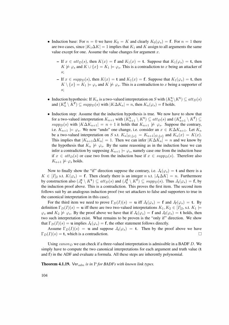
• Induction base: For n = 0 we have K0 = K and clearly K0(ϕs) = f . For n = 1 thereare two cases, since |K1∆K| = 1 implies thatK1 andK assign to all arguments the samevalue except for one. Assume the value changes for argument x.

– If x ∈ attD(s), then K(x) = f and K1(x) = t. Suppose that K1(ϕs) = t, thenK 6|= ϕs and K ∪ {x} = K1 |= ϕs. This is a contradiction to x being an attacker ofs;

– If x ∈ suppD(s), then K(x) = t and K1(x) = f . Suppose that K1(ϕs) = t, thenK \ {x} = K1 |= ϕs and K 6|= ϕs. This is a contradiction to x being a supporter ofs;

• Induction hypothesis: IfKn is a two-valued interpretation on S with (Ktn\Kt) ⊆ attD(s)

and (Kfn \Kf ) ⊆ suppD(s) with |K∆Kn| = n, then Kn(ϕs) = f holds.

• Induction step: Assume that the induction hypothesis is true. We now have to show thatfor a two-valued interpretation Kn+1 with (Kt

n+1 \Kt) ⊆ attD(s) and (Kfn+1 \Kf ) ⊆

suppD(s) with |K∆Kn+1| = n + 1 it holds that Kn+1 6|= ϕs. Suppose the contrary,i.e. Kn+1 |= ϕs. We now “undo” one change, i.e. consider an x ∈ K∆Kn+1. Let Kn

be a two-valued interpretation on S s.t. Kn|S\{x} = Kn+1|S\{x} and Kn(x) = K(x).This implies that |Kn+1∆Kn| = 1. Then we can infer |K∆Kn| = n and we know bythe hypothesis that Kn 6|= ϕs. By the same reasoning as in the induction base we caninfer a contradiction by supposing Kn+1 |= ϕs, namely case one from the induction baseif x ∈ attD(s) or case two from the induction base if x ∈ suppD(s). Therefore alsoKn+1 6|= ϕs holds.

Now to finally show the “if” direction suppose the contrary, i.e. Jt(ϕs) = t and there is aK ∈ [I]2 s.t. K(ϕs) = f . Then clearly there is an integer n s.t. |Jt∆K| = n. Furthermoreby construction also (Jt

t \Kt) ⊆ attD(s) and (J ft \Kf ) ⊆ suppD(s). Thus Jt(ϕs) = f , by

the induction proof above. This is a contradiction. This proves the first item. The second itemfollows suit by an analogous induction proof (we set attackers to false and supporters to true inthe canonical interpretation in this case).

For the third item we need to prove ΓD(I)(s) = u iff Jt(ϕs) = f and Jf (ϕs) = t. Bydefinition ΓD(I)(s) = u iff there are two two-valued interpretations K1,K2 ∈ [I]2, s.t. K1 |=ϕs and K2 6|= ϕs. By the proof above we have that if Jt(ϕs) = f and Jf (ϕs) = t holds, thentwo such interpretation exist. What remains to be proven is the “only if” direction. We showthat ΓD(I)(s) = u implies Jt(ϕs) = f , the other statement follows directly.

Assume ΓD(I)(s) = u and suppose Jt(ϕs) = t. Then by the proof above we haveΓD(I)(s) = t, which is a contradiction.

Using canonD we can check if a three-valued interpretation is admissible in a BADFD. Wesimply have to compute the two canonical interpretations for each argument and truth value (tand f ) in the ADF and evaluate a formula. All these steps are inherently polynomial.

Theorem 4.1.19. Veradm is in P for BADFs with known link types.

104

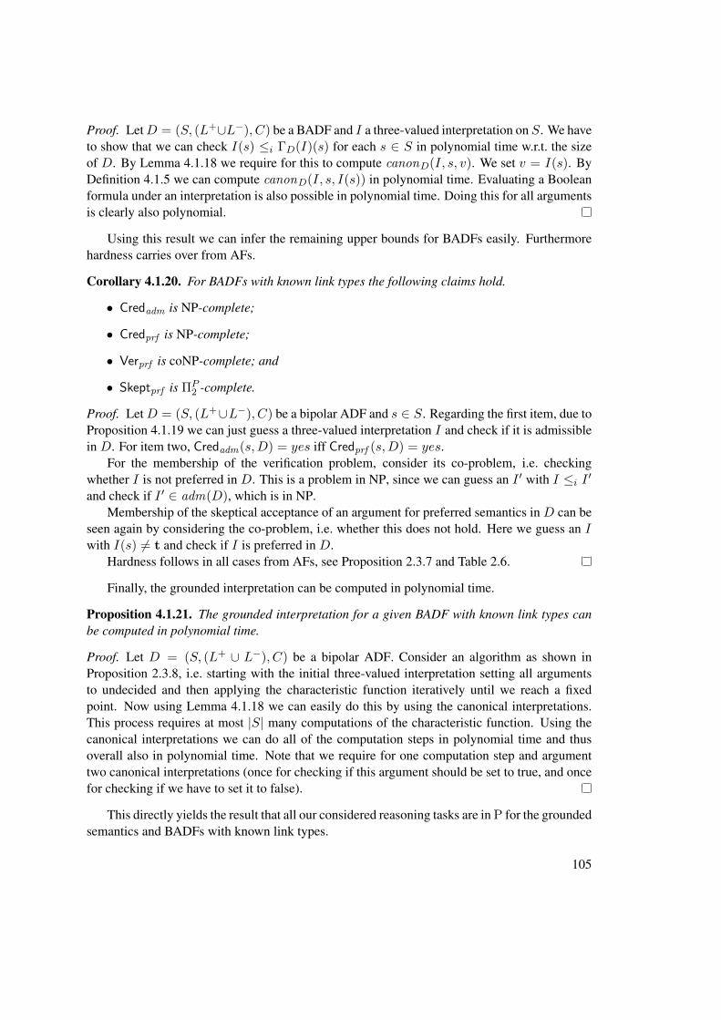
Proof. LetD = (S, (L+∪L−), C) be a BADF and I a three-valued interpretation on S. We haveto show that we can check I(s) ≤i ΓD(I)(s) for each s ∈ S in polynomial time w.r.t. the sizeof D. By Lemma 4.1.18 we require for this to compute canonD(I, s, v). We set v = I(s). ByDefinition 4.1.5 we can compute canonD(I, s, I(s)) in polynomial time. Evaluating a Booleanformula under an interpretation is also possible in polynomial time. Doing this for all argumentsis clearly also polynomial.

Using this result we can infer the remaining upper bounds for BADFs easily. Furthermorehardness carries over from AFs.

Corollary 4.1.20. For BADFs with known link types the following claims hold.

• Credadm is NP-complete;

• Credprf is NP-complete;

• Verprf is coNP-complete; and

• Skeptprf is ΠP2 -complete.

Proof. LetD = (S, (L+∪L−), C) be a bipolar ADF and s ∈ S. Regarding the first item, due toProposition 4.1.19 we can just guess a three-valued interpretation I and check if it is admissiblein D. For item two, Credadm(s,D) = yes iff Credprf (s,D) = yes.

For the membership of the verification problem, consider its co-problem, i.e. checkingwhether I is not preferred in D. This is a problem in NP, since we can guess an I ′ with I ≤i I ′and check if I ′ ∈ adm(D), which is in NP.

Membership of the skeptical acceptance of an argument for preferred semantics in D can beseen again by considering the co-problem, i.e. whether this does not hold. Here we guess an Iwith I(s) 6= t and check if I is preferred in D.

Hardness follows in all cases from AFs, see Proposition 2.3.7 and Table 2.6.

Finally, the grounded interpretation can be computed in polynomial time.

Proposition 4.1.21. The grounded interpretation for a given BADF with known link types canbe computed in polynomial time.

Proof. Let D = (S, (L+ ∪ L−), C) be a bipolar ADF. Consider an algorithm as shown inProposition 2.3.8, i.e. starting with the initial three-valued interpretation setting all argumentsto undecided and then applying the characteristic function iteratively until we reach a fixedpoint. Now using Lemma 4.1.18 we can easily do this by using the canonical interpretations.This process requires at most |S| many computations of the characteristic function. Using thecanonical interpretations we can do all of the computation steps in polynomial time and thusoverall also in polynomial time. Note that we require for one computation step and argumenttwo canonical interpretations (once for checking if this argument should be set to true, and oncefor checking if we have to set it to false).

This directly yields the result that all our considered reasoning tasks are in P for the groundedsemantics and BADFs with known link types.

105

4.2 Algorithms for ADFs

In this section we generalize our search algorithms from Section 3 to (B)ADFs and the preferredsemantics and present a backbone algorithm for the grounded semantics.

4.2.1 Search Algorithm for Preferred Semantics

We instantiate our generic Algorithm 1 with ADFs, by slightly adapting it. For preferred seman-tics we use admissible interpretations as our base semantics. The reason for this is simply thatby definition we have max<i(adm(D)) = prf (D) for any ADF D. We begin by defining thetwo relevant sets of interpretations.

Definition 4.2.1. Let D = (S,L,C) be an ADF, S ⊆ prf (D), X ∈ prf (D). Define thefollowing two subsets of preferred interpretations.

• InterpExcl(D,S) = {I ∈ adm(D) | @I ′ ∈ S s.t. I ≤i I ′};

• GreaterInterp(D,X) = {I ∈ adm(D) | X <i I}.

These two sets of three-valued interpretations clearly mirror the sets of the generic algorithmfrom Section 3. That is the two sets contain admissible interpretations and InterpExcl(D,S)restricts to those, which are not smaller or equal to the ones in S, w.r.t. ≤i. Whereas the setGreaterInterp(D,X) contains admissible interpretations, which are greater to X w.r.t. <i.

It is now straightforward to instantiate Algorithm 1 with preferred semantics for ADFs. Weshow this in Algorithm 14.

We can directly infer all desired properties for our algorithm shown earlier for AFs from theproof of Theorem 3.3.4.

Corollary 4.2.1. Let D = (S,L,C) be an ADF, a ∈ S, M ∈ {Cred, co-Skept,Enum}. Then

• Preferred-ADF(D, a,M) terminates;

• Credprf (a,D) = yes iff Preferred-ADF(D, a,Cred) returns yes;

• Skeptprf (a,D) = yes iff Preferred-ADF(D, a, co-Skept) returns no;

• Preferred-ADF(D, a,Enum) returns prf (F ) = S.

Considering the running time of Algorithm 14 we state the number of membership checks inLine 2 and Line 3 the algorithm executes in the worst case. We view these two lines as functioncalls. The following proposition follows directly from Proposition 3.3.5.

Proposition 4.2.2. Let D = (S,L,C) be an ADF, a ∈ S. The number of function calls (Line 2and Line 3 of Algorithm 14) of Preferred-ADF(D, a,M) for M ∈ {Cred, co-Skept,Enum} isO(|S| · |prf (D)|).

106

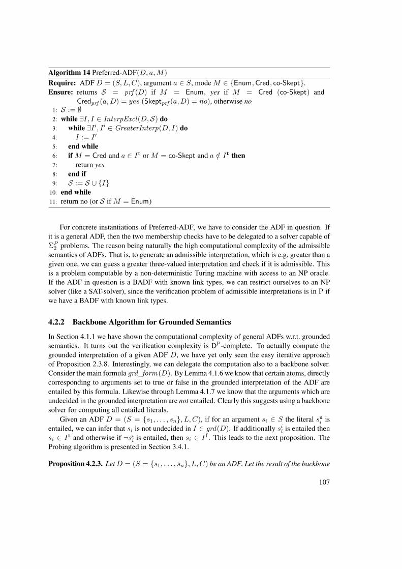
Algorithm 14 Preferred-ADF(D, a,M)

Require: ADF D = (S,L,C), argument a ∈ S, mode M ∈ {Enum,Cred, co-Skept}.Ensure: returns S = prf (D) if M = Enum, yes if M = Cred (co-Skept) and

Credprf (a,D) = yes (Skeptprf (a,D) = no), otherwise no1: S := ∅2: while ∃I, I ∈ InterpExcl(D,S) do3: while ∃I ′, I ′ ∈ GreaterInterp(D, I) do4: I := I ′

5: end while6: if M = Cred and a ∈ It or M = co-Skept and a /∈ It then7: return yes8: end if9: S := S ∪ {I}


For concrete instantiations of Preferred-ADF, we have to consider the ADF in question. Ifit is a general ADF, then the two membership checks have to be delegated to a solver capable ofΣP

2 problems. The reason being naturally the high computational complexity of the admissiblesemantics of ADFs. That is, to generate an admissible interpretation, which is e.g. greater than agiven one, we can guess a greater three-valued interpretation and check if it is admissible. Thisis a problem computable by a non-deterministic Turing machine with access to an NP oracle.If the ADF in question is a BADF with known link types, we can restrict ourselves to an NPsolver (like a SAT-solver), since the verification problem of admissible interpretations is in P ifwe have a BADF with known link types.

4.2.2 Backbone Algorithm for Grounded Semantics

In Section 4.1.1 we have shown the computational complexity of general ADFs w.r.t. groundedsemantics. It turns out the verification complexity is DP-complete. To actually compute thegrounded interpretation of a given ADF D, we have yet only seen the easy iterative approachof Proposition 2.3.8. Interestingly, we can delegate the computation also to a backbone solver.Consider the main formula grd_form (D). By Lemma 4.1.6 we know that certain atoms, directlycorresponding to arguments set to true or false in the grounded interpretation of the ADF areentailed by this formula. Likewise through Lemma 4.1.7 we know that the arguments which areundecided in the grounded interpretation are not entailed. Clearly this suggests using a backbonesolver for computing all entailed literals.

Given an ADF D = (S = {s1, . . . , sn}, L, C), if for an argument si ∈ S the literal sui isentailed, we can infer that si is not undecided in I ∈ grd(D). If additionally sii is entailed thensi ∈ It and otherwise if ¬sii is entailed, then si ∈ If . This leads to the next proposition. TheProbing algorithm is presented in Section 3.4.1.

Proposition 4.2.3. LetD = (S = {s1, . . . , sn}, L, C) be an ADF. Let the result of the backbone

107

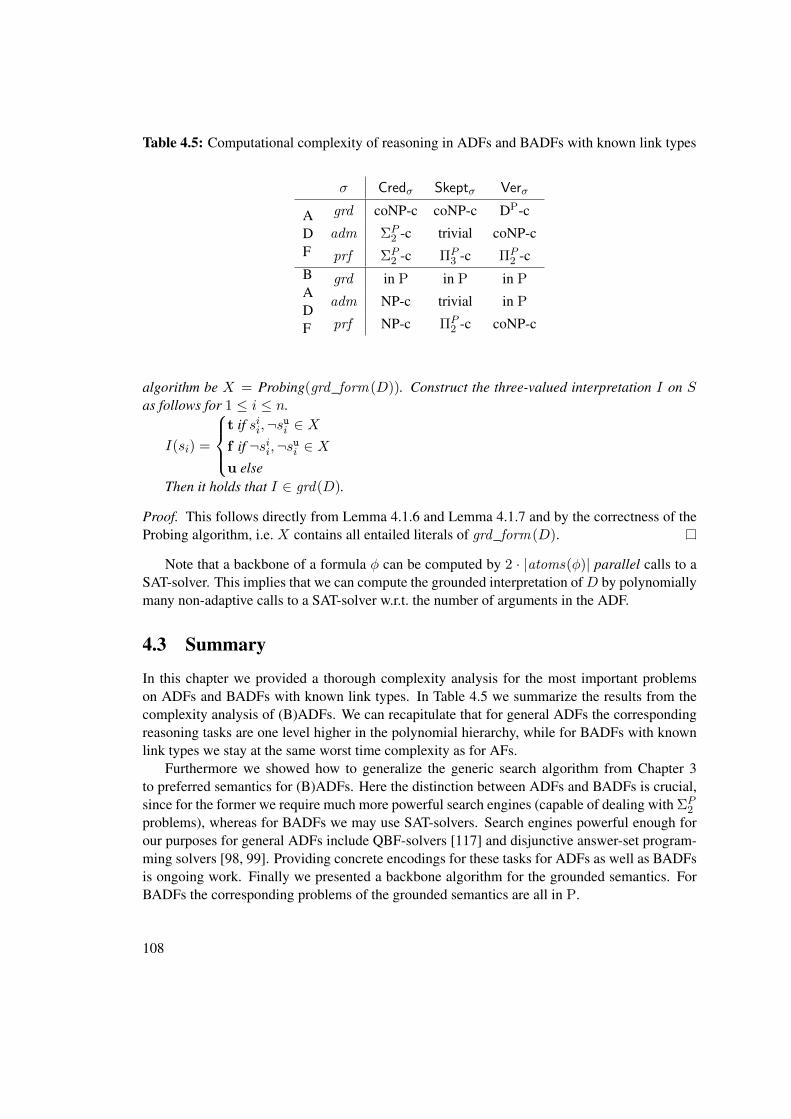
Table 4.5: Computational complexity of reasoning in ADFs and BADFs with known link types

σ Credσ Skeptσ Verσ

ADF

grd coNP-c coNP-c DP-c

adm ΣP2 -c trivial coNP-c

prf ΣP2 -c ΠP

3 -c ΠP2 -c

BADF

grd in P in P in P

adm NP-c trivial in P

prf NP-c ΠP2 -c coNP-c

algorithm be X = Probing(grd_form (D)). Construct the three-valued interpretation I on Sas follows for 1 ≤ i ≤ n.

I(si) =

t if sii,¬sui ∈ Xf if ¬sii,¬sui ∈ Xu else

Then it holds that I ∈ grd(D).

Proof. This follows directly from Lemma 4.1.6 and Lemma 4.1.7 and by the correctness of theProbing algorithm, i.e. X contains all entailed literals of grd_form (D).

Note that a backbone of a formula φ can be computed by 2 · |atoms(φ)| parallel calls to aSAT-solver. This implies that we can compute the grounded interpretation ofD by polynomiallymany non-adaptive calls to a SAT-solver w.r.t. the number of arguments in the ADF.

4.3 Summary

In this chapter we provided a thorough complexity analysis for the most important problemson ADFs and BADFs with known link types. In Table 4.5 we summarize the results from thecomplexity analysis of (B)ADFs. We can recapitulate that for general ADFs the correspondingreasoning tasks are one level higher in the polynomial hierarchy, while for BADFs with knownlink types we stay at the same worst time complexity as for AFs.

Furthermore we showed how to generalize the generic search algorithm from Chapter 3to preferred semantics for (B)ADFs. Here the distinction between ADFs and BADFs is crucial,since for the former we require much more powerful search engines (capable of dealing with ΣP

2

problems), whereas for BADFs we may use SAT-solvers. Search engines powerful enough forour purposes for general ADFs include QBF-solvers [117] and disjunctive answer-set program-ming solvers [98, 99]. Providing concrete encodings for these tasks for ADFs as well as BADFsis ongoing work. Finally we presented a backbone algorithm for the grounded semantics. ForBADFs the corresponding problems of the grounded semantics are all in P.

108

CHAPTER 5Implementation and Empirical

Evaluation

This chapter provides the third major contribution of this thesis, the practical instantiation of ourproposed algorithms in form of executable software programs and their experimental evaluation.Although our algorithms in Chapter 3 satisfy certain appealing theoretic properties, it is not clearfrom theory alone if they are suited for AF problems in concrete implementations.

We implemented the search Algorithm 6 in the software CEGARTIX and the SAT extensionbased algorithms from Section 3.4. Both were evaluated on randomly generated AFs with twoparametrized creation methods. All our tools are available online (see Table 5.3 on page 123).

Therefore we give two contributions in this chapter.

• We provide implementations of our search algorithms in the form of CEGARTIX in Sec-tion 5.1.1 and algorithms based on SAT extensions for AFs in Section 5.1.2;

• and compare these programs with state-of-the-art systems in abstract argumentation inSection 5.2.

The results of the performance analysis for the search algorithms of this chapter have beenpublished in [75, 76, 77]. The results for the algorithms based on SAT extensions have beenpublished in [153].

5.1 System Description

We implemented two prototypical systems for experimenting with our algorithms from Chap-ter 3. The first one, called CEGARTIX, implements the search algorithm Decide (Algorithm 6),including its shortcuts from Section 3.3.4. This algorithm is designed to be well-suited for de-ciding whether an argument is credulously accepted w.r.t. semi-stable or stage semantics, orskeptically accepted w.r.t. preferred, semi-stable or stage semantics. The second system imple-ments the algorithms based on SAT extensions from Section 3.4. We call this set of tools simply

109

SAT extension based algorithms. In particular we implemented an MCS-based algorithm forcomputing credulous and skeptical reasoning w.r.t. semi-stable semantics and enumerating thesemi-stable extensions. Further we implemented also a variant for returning all skeptically ac-cepted arguments of an AF w.r.t. semi-stable semantics and used this implementation with asimple post processor to return the eager extension. Further we implemented the backbone-based algorithm for ideal semantics.

The input language for all our systems follows the format of the well-known system AS-PARTIX [85]. ASPARTIX is an answer-set programming (ASP) [30, 87, 99] approach to solvereasoning tasks for many AF semantics. For specifying an AF the following format is used,which corresponds to so-called facts of an ASP encoding. Given an AF F = (A,R) the inputfor ASPARTIX is

{arg(a). | a ∈ A} ∪ {att(a, b). | (a, b) ∈ R}

Example 5.1.1. Let F = ({a, b, c}, {(a, b), (b, a), (b, c)}) be an AF. Then the ASPARTIX formatwould be

arg(a).arg(b).arg(c).att(a,b).att(b,a).att(b,c).

Our systems support the same input language, with the requirement that each line has atmost one statement (arg or att).

5.1.1 CEGARTIX

CEGARTIX, borrowing terminology from CEGAR-style approaches [49, 50] (counter-exampleguided abstraction refinement) is a C++ implementation for UNIX systems of Algorithm 6(Decide). Briefly put, this algorithm searches for a witness or a counter-example for decidingthe problem at hand. It searches for such a witness or counterexample by computing an initialcandidate, which is complete or admissible for the given AF. The algorithm then computes can-didates which are greater w.r.t. a certain ordering in an iterative fashion. Thus it borrows somemechanics from the CEGAR approach. It is capable of solving the following reasoning tasks foran AF.

• Credulous reasoning with semi-stable and stage semantics; and

• skeptical reasoning with preferred, semi-stable and stage semantics.

These are all problems, in our context, which are complete for the second level of the poly-nomial hierarchy. CEGARTIX employs SAT-solvers to compute the computationally intensivetasks and handles itself the formula generation and SAT-solver calls. Initially, in v0.1, CEGAR-TIX was built on top of MiniSAT [84] v2.2.0. MiniSAT is used in an incremental mode. This

110

means that, if possible, during the computation we retain the solver state after a formula wasfound satisfiable and add further clauses directly to this state without a fresh restart. In v0.2 ofCEGARTIX we additionally support clasp [102] v2.0.5 in a non-incremental mode (as well asremoving incremental solving for MiniSAT). In v0.3 of CEGARTIX we now support arbitrarySAT-solvers as long as they adhere to the input/output of the SAT competitions [108]. In v0.3we provide two variants of CEGARTIX, one, which uses again MiniSAT incrementally and onewithout this feature. CEGARTIX is invoked as follows.

./CEGARTIX file options

The file should contain the AF in the ASPARTIX input format. For the options we supportthe following (v0.3, for other versions see the help option).

• -argument=string specifies which argument should be checked;

• -semantics=string specifies the semantics. Allowed values are pref (default),semi and stage;

• -mode=string is used to define credulous or skeptical reasoning;

• -depthArg=int specifies the bound d for the shortcuts; d ∈ {−1, 0, 1, 2} where d =−1 means no shortcut (Algorithms 7 and 8);

• -oracle=string defines the used SAT-solver. Can be one of miniSAT, clasp, orexternal. The last one requires also the next option;

• -external=string the path for the external SAT-solver; and

• --help or --help-verb prints further help information.

After invocation CEGARTIX prints to standard out the answer to the query with some statis-tics.

5.1.2 SAT Extension based Algorithms

The second implementation within the scope of our thesis is actually a set of tools. They are allbased on SAT extensions as discussed in Section 3.4. The following prototypical programs areimplemented for UNIX systems.

• MCS, solves Enumsem(F ), AllSkeptsem(F ), Credsem(a, F ) and Skeptsem(a, F ) for anAF F = (A,R) and a ∈ A;

• MCS eager, returns the eager extension;

• Backbone ideal, returns the ideal extension.

111

The tool MCS computes the result via an adapted version of CAMUS [115] v1.0.5, a solverfor systematically computing all minimal correction sets of a formula. In the thesis we showedthe variant for AllSkeptsem (Algorithm 11), but the other variants can be directly inferred (justreplace the intersection of the models with a check for credulous or skeptical acceptance or withan enumeration). We note that the current implementation does not feature the optimization withusing a backbone solver for computing all skeptically accepted arguments, but simply enumer-ates the models and computes the intersection. The program is invoked by a simple shell scriptsemi.sh, which invokes a parser for the given AF and the adapted CAMUS.

./semi.sh file options [argument]

Again we provide the options.

• cred cred(ulous) reasoning, requires argument

• skept skept(ical) reasoning, requires argument

• enum enum(eration) of all semi-stable extensions

• allSkept returns all skeptically accepted arguments

• argument the argument for the query

The MCS eager tool calls MCS for computing all skeptically accepted arguments w.r.t. semi-stable semantics and then invokes a post-processor to find the eager extension. This post pro-cessor computes the restricted characteristic function (see Definition 2.3.16). We implementedthis computation with a simple ASP encoding. The MCS eager tool is again wrapped in a smallshell script eager.sh and invoked by

./eager.sh file

which returns the eager extension of the AF encoded as ASP facts in file. The postprocessingstep is achieved via an ASP call to clingo [98] v3.0.4. Finally Backbone ideal computes the idealextension of a given AF. The backbone solver JediSAT [159] v0.2 beta is used to compute allcredulously accepted arguments w.r.t. admissibility, i.e. AllCredadm(F ) for an AF F . The toolthen computes the ideal extension via the Algorithm 13 from [62]. This is again achieved withan ASP encoding. It is very similar to the one used for the eager extension, just the AF has to beslightly adapted. The invocation is again simple, and handled by the shell script ideal.sh.

./ideal.sh file

The translation from an AF to a formula is handled in all tools of this section by a C++program, which was adapted from CEGARTIX.

112

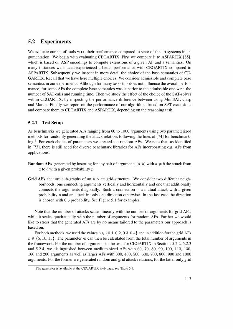
5.2 Experiments

We evaluate our set of tools w.r.t. their performance compared to state-of-the art systems in ar-gumentation. We begin with evaluating CEGARTIX. First we compare it to ASPARTIX [85],which is based on ASP encodings to compute extensions of a given AF and a semantics. Onmany instances we indeed experienced a better performance with CEGARTIX compared toASPARTIX. Subsequently we inspect in more detail the choice of the base semantics of CE-GARTIX. Recall that we have here multiple choices. We consider admissible and complete basesemantics in our experiments. Although for many tasks this does not influence the overall perfor-mance, for some AFs the complete base semantics was superior to the admissible one w.r.t. thenumber of SAT calls and running time. Then we study the effect of the choice of the SAT-solverwithin CEGARTIX, by inspecting the performance difference between using MiniSAT, claspand March. Finally we report on the performance of our algorithms based on SAT extensionsand compare them to CEGARTIX and ASPARTIX, depending on the reasoning task.

5.2.1 Test Setup

As benchmarks we generated AFs ranging from 60 to 1000 arguments using two parameterizedmethods for randomly generating the attack relation, following the lines of [74] for benchmark-ing.1 For each choice of parameters we created ten random AFs. We note that, as identifiedin [73], there is still need for diverse benchmark libraries for AFs incorporating e.g. AFs fromapplications.

Random AFs generated by inserting for any pair of arguments (a, b) with a 6= b the attack froma to b with a given probability p.

Grid AFs that are sub-graphs of an n × m grid-structure. We consider two different neigh-borhoods, one connecting arguments vertically and horizontally and one that additionallyconnects the arguments diagonally. Such a connection is a mutual attack with a givenprobability p and an attack in only one direction otherwise. In the last case the directionis chosen with 0.5 probability. See Figure 5.1 for examples.

Note that the number of attacks scales linearly with the number of arguments for grid AFs,while it scales quadratically with the number of arguments for random AFs. Further we wouldlike to stress that the generated AFs are by no means tailored to the parameters our approach isbased on.

For both methods, we used the values p ∈ {0.1, 0.2, 0.3, 0.4} and in addition for the grid AFsn ∈ {5, 10, 15}. The parameter m can then be calculated from the total number of arguments inthe framework. For the number of arguments in the tests for CEGARTIX in Sections 5.2.2, 5.2.3and 5.2.4, we distinguished between medium-sized AFs with 60, 70, 80, 90, 100, 110, 130,160 and 200 arguments as well as larger AFs with 300, 400, 500, 600, 700, 800, 900 and 1000arguments. For the former we generated random and grid attack relations, for the latter only grid

1The generator is available at the CEGARTIX web page, see Table 5.3.

113

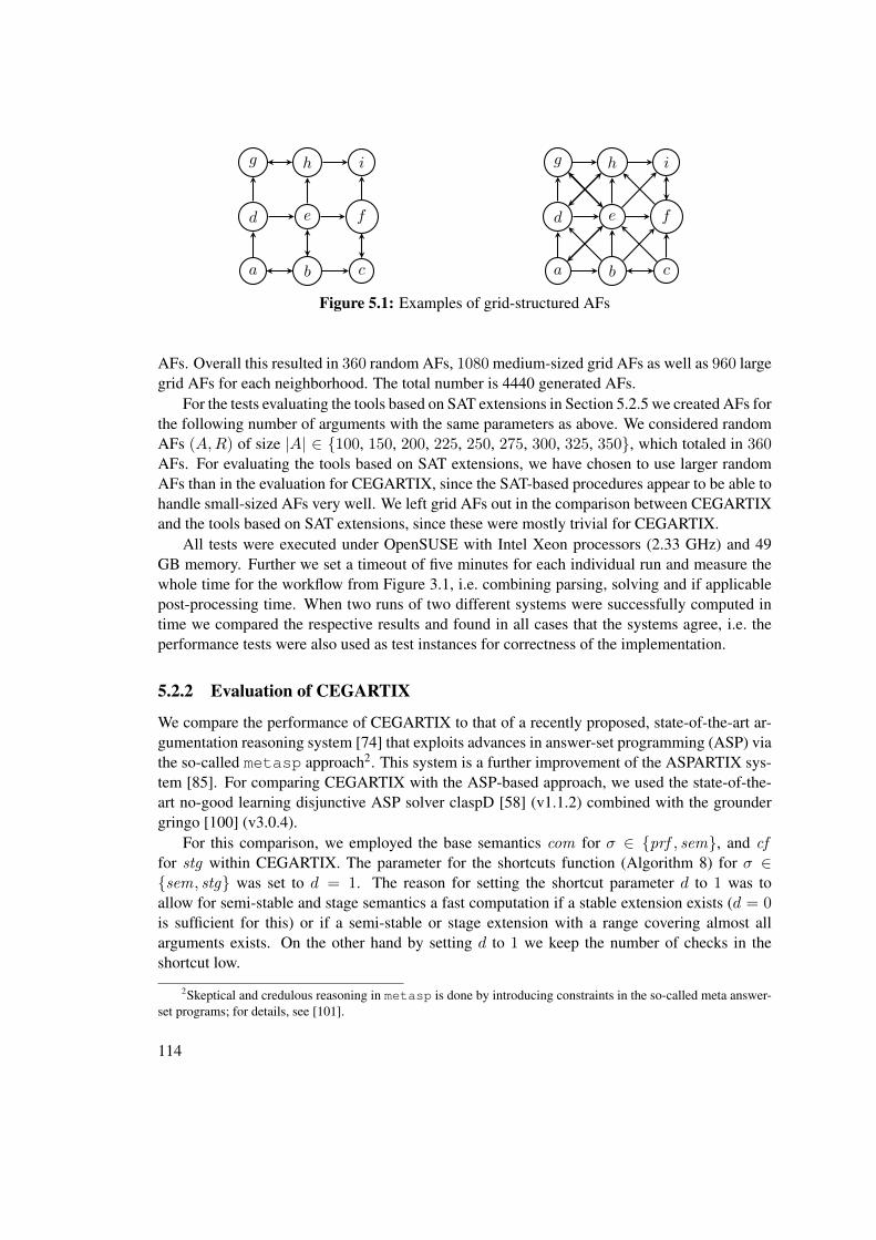
a b c

d e f

g h i

a b c

d e f

g h i

Figure 5.1: Examples of grid-structured AFs

AFs. Overall this resulted in 360 random AFs, 1080 medium-sized grid AFs as well as 960 largegrid AFs for each neighborhood. The total number is 4440 generated AFs.

For the tests evaluating the tools based on SAT extensions in Section 5.2.5 we created AFs forthe following number of arguments with the same parameters as above. We considered randomAFs (A,R) of size |A| ∈ {100, 150, 200, 225, 250, 275, 300, 325, 350}, which totaled in 360AFs. For evaluating the tools based on SAT extensions, we have chosen to use larger randomAFs than in the evaluation for CEGARTIX, since the SAT-based procedures appear to be able tohandle small-sized AFs very well. We left grid AFs out in the comparison between CEGARTIXand the tools based on SAT extensions, since these were mostly trivial for CEGARTIX.

All tests were executed under OpenSUSE with Intel Xeon processors (2.33 GHz) and 49GB memory. Further we set a timeout of five minutes for each individual run and measure thewhole time for the workflow from Figure 3.1, i.e. combining parsing, solving and if applicablepost-processing time. When two runs of two different systems were successfully computed intime we compared the respective results and found in all cases that the systems agree, i.e. theperformance tests were also used as test instances for correctness of the implementation.

5.2.2 Evaluation of CEGARTIX

We compare the performance of CEGARTIX to that of a recently proposed, state-of-the-art ar-gumentation reasoning system [74] that exploits advances in answer-set programming (ASP) viathe so-called metasp approach2. This system is a further improvement of the ASPARTIX sys-tem [85]. For comparing CEGARTIX with the ASP-based approach, we used the state-of-the-art no-good learning disjunctive ASP solver claspD [58] (v1.1.2) combined with the groundergringo [100] (v3.0.4).

For this comparison, we employed the base semantics com for σ ∈ {prf , sem}, and cffor stg within CEGARTIX. The parameter for the shortcuts function (Algorithm 8) for σ ∈{sem, stg} was set to d = 1. The reason for setting the shortcut parameter d to 1 was toallow for semi-stable and stage semantics a fast computation if a stable extension exists (d = 0is sufficient for this) or if a semi-stable or stage extension with a range covering almost allarguments exists. On the other hand by setting d to 1 we keep the number of checks in theshortcut low.

2Skeptical and credulous reasoning in metasp is done by introducing constraints in the so-called meta answer-set programs; for details, see [101].

114

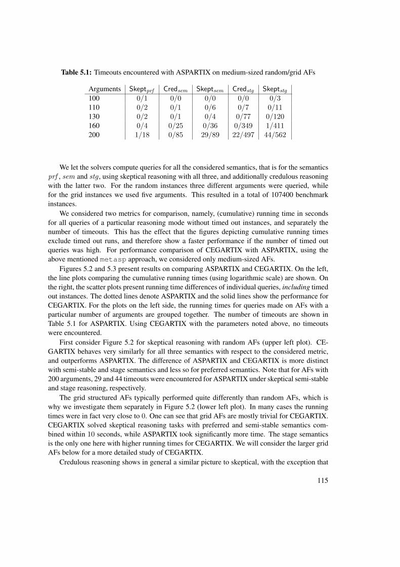
Table 5.1: Timeouts encountered with ASPARTIX on medium-sized random/grid AFs

Arguments Skeptprf Credsem Skeptsem Credstg Skeptstg100 0/1 0/0 0/0 0/0 0/3110 0/2 0/1 0/6 0/7 0/11130 0/2 0/1 0/4 0/77 0/120160 0/4 0/25 0/36 0/349 1/411200 1/18 0/85 29/89 22/497 44/562

We let the solvers compute queries for all the considered semantics, that is for the semanticsprf , sem and stg , using skeptical reasoning with all three, and additionally credulous reasoningwith the latter two. For the random instances three different arguments were queried, whilefor the grid instances we used five arguments. This resulted in a total of 107400 benchmarkinstances.

We considered two metrics for comparison, namely, (cumulative) running time in secondsfor all queries of a particular reasoning mode without timed out instances, and separately thenumber of timeouts. This has the effect that the figures depicting cumulative running timesexclude timed out runs, and therefore show a faster performance if the number of timed outqueries was high. For performance comparison of CEGARTIX with ASPARTIX, using theabove mentioned metasp approach, we considered only medium-sized AFs.

Figures 5.2 and 5.3 present results on comparing ASPARTIX and CEGARTIX. On the left,the line plots comparing the cumulative running times (using logarithmic scale) are shown. Onthe right, the scatter plots present running time differences of individual queries, including timedout instances. The dotted lines denote ASPARTIX and the solid lines show the performance forCEGARTIX. For the plots on the left side, the running times for queries made on AFs with aparticular number of arguments are grouped together. The number of timeouts are shown inTable 5.1 for ASPARTIX. Using CEGARTIX with the parameters noted above, no timeoutswere encountered.

First consider Figure 5.2 for skeptical reasoning with random AFs (upper left plot). CE-GARTIX behaves very similarly for all three semantics with respect to the considered metric,and outperforms ASPARTIX. The difference of ASPARTIX and CEGARTIX is more distinctwith semi-stable and stage semantics and less so for preferred semantics. Note that for AFs with200 arguments, 29 and 44 timeouts were encountered for ASPARTIX under skeptical semi-stableand stage reasoning, respectively.

The grid structured AFs typically performed quite differently than random AFs, which iswhy we investigate them separately in Figure 5.2 (lower left plot). In many cases the runningtimes were in fact very close to 0. One can see that grid AFs are mostly trivial for CEGARTIX.CEGARTIX solved skeptical reasoning tasks with preferred and semi-stable semantics com-bined within 10 seconds, while ASPARTIX took significantly more time. The stage semanticsis the only one here with higher running times for CEGARTIX. We will consider the larger gridAFs below for a more detailed study of CEGARTIX.

Credulous reasoning shows in general a similar picture to skeptical, with the exception that

115

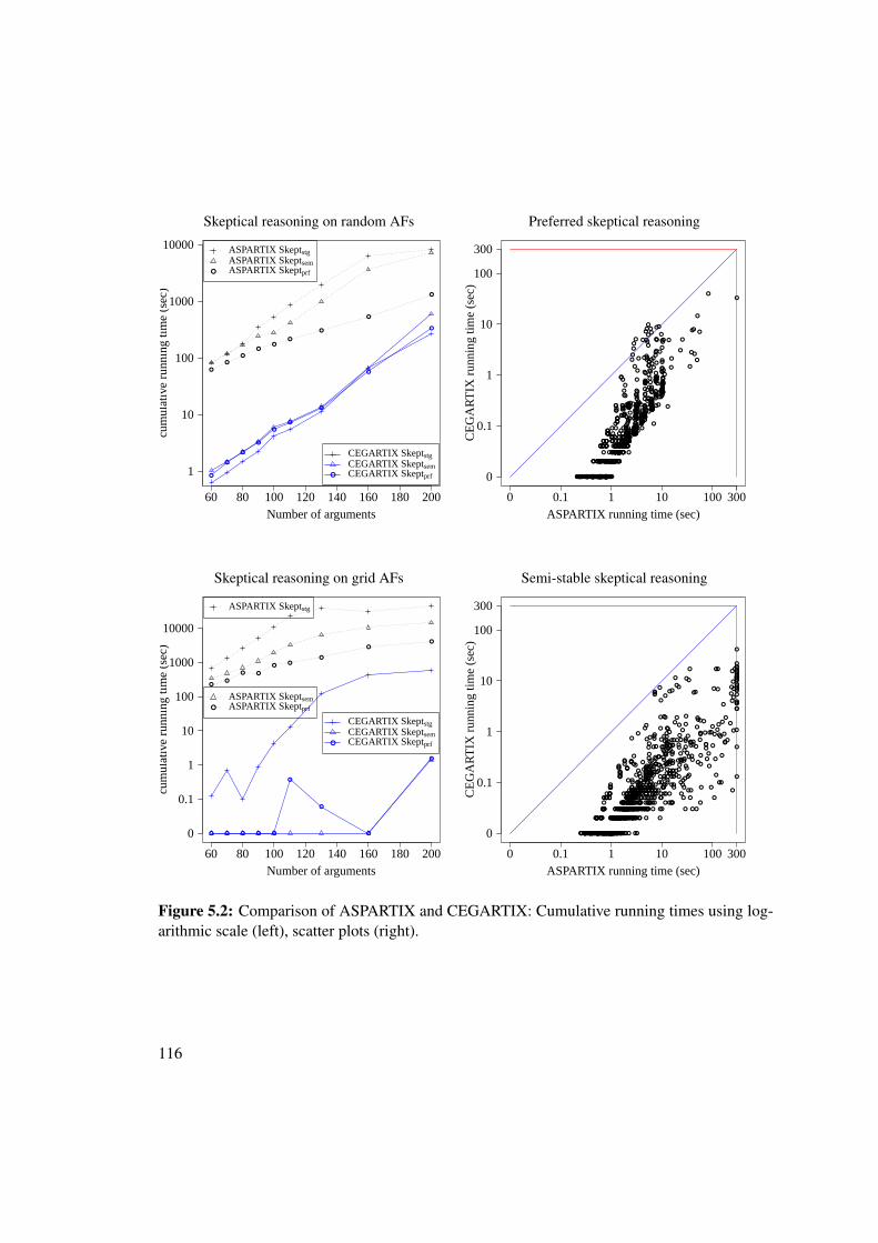
Skeptical reasoning on random AFs

Number of arguments

cum

ulat

ive

runn

ing

time

(sec

)

●

●

●

●●

●

●

●

●

●

●

●

●

●

●

●

●

●

1

10

100

1000

10000

60 80 100 120 140 160 180 200

●

ASPARTIX SkeptstgASPARTIX SkeptsemASPARTIX Skeptprf

●

CEGARTIX SkeptstgCEGARTIX SkeptsemCEGARTIX Skeptprf

Preferred skeptical reasoning

ASPARTIX running time (sec)

CE

GA

RT

IX r

unni

ng ti

me

(sec

)●●● ●●●

●●●

●●●●●●●●●●

●

●●●●

●●●

●●●

●●●

●

●

●

●

●●●●●

●

●

●

●●●

●

●

●

●

●

●

●

●

●●

●●

●

●

●

●●●

●●●●

●●

●●●●●●●

●

●

●

●●

●

●●

●

●● ●

●●●

●

●

●●●●●●●●●●●●●●●●●●●●●●●●

●

●

●

●

●

●

●

●

●●●

●

●●

●

●●●●●●

●●●

●●●

●

●●

●●

●●●

●

●●●

●

●

●●●●

●

●●●

●●

●●

●

●

●●

●

●

●

●

●

●●

●●

●

●●

●

●

●

●●

●●●

●●●●●●

●

●●●

●

●● ●●●

●●●●●●

●●

●

●●●●●●●●●●●●●●●●●

●

●●●

●●

●

●

●

●

●

●

●

●●

●

●●

●●

●●

●

●●

●

●●

●

●

●

●

●

●

●

●●

●

●

●

●●

●●

●

●

●

●

●

●

●

●

●

●

●

●

●●

●

●●

●●

●

●

●●●

●

●●

●●

●●●

●

●

●

●

●●

●

●

●

●●●

●

●●

●●

●●●●●●●●

●●

●●●●●●●●●●●

●

●●●

●

●

●

●

●

●

●

●●

●

●

●

●

●

●

●

●

●

●

●

●

●●●

●

●

●

●

●

●●

●

●

●

●

●●

●

●

●

●●●

●

●

●

●●

●●●

●●●

●

●●

●

●

●

●●

●●

●

●●

●

●●

●●

●

●

●

●●●

●

●●

●

●

●

●

●

●

●

●●●●

●

●●●●●●●●●●●●

●●●●

●●

●

●

●●●●

●

●

●

●●●

●●

●

●

●

●

●

●

●

●

●

●●

●

●

●

●

●

●

●

●

●

●

●

●●

●

●

●

●

●

●

●

●

●

●

●

●

●

●

●

●

●

●

●

●

●

●

●

●

●

●

●

●

●

●

●

●

●

●

●

●

●●

●●

●

●

●

●

●

●

●

●

●●

●●

●

●

●

●

●

●●

●

●

●

●

●

●

●

●

●

●

●

●

●

●

●

●

●●

●●●●●

●●

●

●●

●●

●●

●

●

●

●●● ●●●●●●●●●●●●●●●●●●●●●●●●●●● ●●●●●●●●●●●●●●●●●●●●●●●●●●●●●● ●●●●

●

●

●●●

●●●

●●●

●●●●●●●●●●●●●●● ●●●●●●●●●●●●●●●●●●●●●●●●●●●●●●●●●●●●●●●●●●●●●● ●●●●●●●●●●●●●● ●●

●●●●

●●

●

●●●●●●●●●●●●●●●●●●●●● ●●●●●●●●●●●

●

●●●

●

●

●

●

●

●

●

●

●

●

●

●●

●● ●●●●●●●●●●●●●●●●●●●●●●●●●●●●●●

●●●●●●●●●

●●●

●●●●●●●●●●●●●●●●●● ●

●

●

●

●

●

●

●

●●

●

●●●●●●

●

●●●

●●●

●●

●●●●

●●●●●●●●●●●●●●●●

●

●●●●●●●●●●●●●

●

●

●●●●●●●●●●●●●

●

●●●●●●●●●●

●

●●●

●●●●●●

●●●

●●●

●●●

●●●●●●●●

●

●

●

●●●● ●

●

●

●●●●

●

●●●●●●●●●●●●●

●

●●

●

●

●●

●

●

●

●●●●●●●

●●

●●

●

●●●●

●

●

●

●●

●●

●●●●●●

●●●●●●●●●●●●●●●●●●●●●

●

●●●●●●●●

0

0.1

1

10

100

300

0 0.1 1 10 100 300

Skeptical reasoning on grid AFs

Number of arguments

cum

ulat

ive

runn

ing

time

(sec

)

●●

● ●

●●

●

●

●

● ● ● ● ●

●

●

●

●

0

0.1

1

10

100

1000

10000

60 80 100 120 140 160 180 200

ASPARTIX Skeptstg

●

ASPARTIX SkeptsemASPARTIX Skeptprf

●

CEGARTIX SkeptstgCEGARTIX SkeptsemCEGARTIX Skeptprf

Semi-stable skeptical reasoning


CE

GA

RT

IX r

unni

ng ti

me

(sec

)

●● ●●●●

●●●

●●●●●●● ●●●●● ●●●

●●●

●●●

●●●

●●●

●

●

●

●

●●●

●

●

●●●

●●●

●

●

●

●●

●

●

●

●

●●●

●●●

●●●

●●●

●●●●●●●● ●●●●

● ●●

●

● ●

●

●

●●● ●●●●

●●

●●●●

●● ●●●●●● ●●●●●●

●

●

● ●

●

●

●

●

●

●

● ●

●

●● ●

●●●●●●

●●●

●● ●●

● ●

●

●

●

●

●

●

●●●

●

●● ●

●

●

●

●

●

●●

●●

●●

●

●

●●

●

●

●

●●

●●

●

●

●●

● ●●

●

●●

●●●

●● ●

●●●

●●●

● ●●

●●

●●

●●●●●

●●

●

●

●

●●●●

●●

●●●

● ●●

●●●●

●●●

●

●●

● ●●

●

●●

●

●

●

●

●

●

●

●

●

●

●●

●●

●

●

●

●

●

●

●

●

●

●

●

●

●

●

●

●

●

●

●

● ●●

●●●

●

●

●●

●

●

● ●

●

●●

●

●

●

●

●

●●

●

●●

●●●

●●●

●●

●●

●

●

●

●

●

●

●

●●

●●

●

●

●●

●●

●●●●

●●

●●

●●●

●

●

●●●●

●

●●●

●

●

●

●

●●●

●

●

●

●

●

●

●

●

●

●

●

●●

●

●

●

●

●

●●

● ●●

●

●

●

●

●

●

●●

●

●

●

●

●●

●

●●●

●

●

●

●

●

●

●

●

●

●

●

●

●

●

●●

●

●●

●●

●

●

●

●

●

●

●

●

●

●

●

●

● ●

●●●

●

●●

●

● ●

●

● ●

●

●● ●●

●●●●

● ●

●

●

●

●

●●●

●

●

● ●

●●

●

●

●●

●●

●

●●

●

●

●

●

●●●

●

●

●

●

●●

●

●

●

●

●●

●

●

●●

●

●

● ●

●●

●

●

●

●

●

●

●

●

●

● ●● ●●●

●

●

●

●

●

●

●

●●

●

●

●●

●

●

●

●

●

●

●

●

●

●

●●

●

●

●

●

●

●

●

●

●●

●

●●

●

●

●

●●●

●

●

●

●● ●

●

●●

●

●

●●●

●●● ●

●

●

●

●

●

●

●●● ●●●●●●●●●●●●●●●●●●●●●●●●●●● ●●●●●● ●●●●●●●●●●●●

●●●

●●●

●●●

●●● ●●●●●●

●●●

●●●

●●●

●●●●●●● ●●●●● ●●●●●●●●● ●●●●●●●●●●●●●●●●●●●●●●●●●●●●●●●●●●●●●●●●●●●●● ●●●●●●●●● ●● ●

●●●

●● ●●●●●●● ● ●●●●●●●● ●● ●●●● ●●●●●●

●

●

●

● ●

●

●

●

●

●

●

●

●

●

●

●●●●

●●

● ●● ●● ●●●●●●●●●● ●

●●

●●● ●●●●●●●● ●●●●

●●● ●●●●●●

●●●

●●●●●●●●●●●●●●● ●●● ●●●

● ●

●● ●●●●●●●●●●●●●

●

●●●

●●●●●●

●●●●●●●●●●●

●●

●●●●● ●●●●●●● ●●

●

●

●

● ●●

● ●●●●● ●● ● ●

●

●●●● ●●● ●●●

●●

●●●●

●●●●●●

●●●

●●●

●●●

●●●●●● ●● ●

●●●

● ●●

●●●●●● ●● ●●● ●

●

●● ● ●●● ●

●

●● ●

●

●●

●

● ●

●●

●

●●

●

●

●

●●●●● ●●

●●●

●●

● ● ●

●

●

●

●●● ●

●●

●●●

●●

●●

●●●

●●● ●●

● ●●●

●●●

● ●●●●●

0

0.1

1

10

100

300

0 0.1 1 10 100 300

Figure 5.2: Comparison of ASPARTIX and CEGARTIX: Cumulative running times using log-arithmic scale (left), scatter plots (right).

116

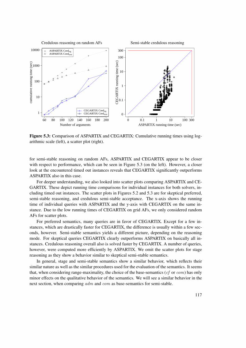
Credulous reasoning on random AFs

Number of arguments

cum

ulat

ive

runn

ing

time

(sec

)

1

10

100

1000

10000

60 80 100 120 140 160 180 200

ASPARTIX CredstgASPARTIX Credsem

CEGARTIX CredstgCEGARTIX Credsem

Semi-stable credulous reasoning


CE

GA

RT

IX r

unni

ng ti

me

(sec

)●●●●●●

●●●

●●●●●●●●●●●●●● ●

●

●

●

●●●

●●●

●●●

●

●●

●

●

●

●

●●

●●●

●

●

●●●●

●●●

●

●

● ●●

●

●●●

●●

●

●●●

●

●

●●●●

●●

●●

●●●

●●

●●

●●●●●●

●

●●●●●●●

●●

●

●●●●●●●●

●

●●●●

●

●●●●

●

●●

●

●●●●●●●

●●●●●●

●●●

●●

●

●

●

●

●●●●

●

●

●●●

●

●

●●

●

●

●

●●

●

●

●

●

●

●●●●●

●●

●●

●

●●●●●

●●

●

●●●●

●●●

●●●●●●

●●●

●

●●

●●●●

●●●●●

●

●

●

●●●●●●●●●

●●●

●

●●

●●●●●●

●

●

●●●

●

●●

●●

●●

●●●

●

●

●

●

●

●

●

●

●

●

●

● ●

●●

●

●

●●

●

●

●●●●●

●

●●

●

●

●

●●

●

●

●

●●

●●●

●

●●●

●

●●●

●●

●

●●

●

●

●

●●

●

●●●●

●

●

●●

●●

●

●●●

●

●●●●●

●

●●

●

●●

●●

●●●●●●●●●●●●●

●

●

●

●

●

●

●

●

●

●

●

●

●●

●

●

●

●

●●

●

●

●●

●

●

●

●

●

●

●

●

●

●

●

●

●

●

●●

●

●

●

●

●

●

●

●

●●

●●

●

●

●

●●

●

●

●●

●●●●

●

●

●

●

●

●

●

●●

●

●

●

●

●●

●

●

●

●

●

●

●

●●

●●●●●

●

●

●

●●●

●

●●

●●

●

●●

●●

●

●●

●

●●

●

●●●

●● ●

●

●

●

●

●

●

●

●

●●

●

●

●

●

●●

●

●

●

●●

●

●●

●

●

●

●

●●

●●

●

●●

●

●

●

●●

●

●

●

●

●

●●●

●

●●

●

●

●

●

●

●

●

●●

●

●●

●

●

●

●

●

●

●

●

●

●

●●

●●

●

●

●

●

●

●

●

●

●

●

●●

●●●●●

●●●

●

●

●

●

●●

●●

●

●

●●

●

●

●

●

●●

●●

●●●●●●●●●● ●●●●●●

●●●

●●●

●●●

●●●●●●●●●●●●●●● ●●●●●●●●●●●●●●●●●●●●●●●●●●●●●●●●● ●●●

●●●

●●●●●●●●●●●●●●●●●●●●●●●● ●●●●●●●

●●

●●●●●●●●

●

●●●●

●

●●●●

●

●●

●●●●●●●●●●●●●●●●●●●●●●●●●●●●●●

●●●●●● ●●●

●

●●●●●●●●●●●●●●●●●

●●●

●●

●●●●

●●●●●●●●●●●●●●●●●●●●●●●●●●●●●●

●●●●●●●●●●●●●●●●●●●●●●●●●

●

●●●●

●●●●●●●●

●●●

●●●●●●●●●●●

●●

●●

●●

●

●●

●●

●

●

●●

●●

●●●

●

●

●●●

●●

●●●

●●

●

●●

●

●

●

●●

●●●●●●●●●

●

●●

●●●●

●●●●

●●●●●●●●●●●●●●●●●●●●●●●●●●●●●●

0

0.1

1

10

100

300

0 0.1 1 10 100 300

Figure 5.3: Comparison of ASPARTIX and CEGARTIX: Cumulative running times using log-arithmic scale (left), a scatter plot (right).

for semi-stable reasoning on random AFs, ASPARTIX and CEGARTIX appear to be closerwith respect to performance, which can be seen in Figure 5.3 (on the left). However, a closerlook at the encountered timed out instances reveals that CEGARTIX significantly outperformsASPARTIX also in this case.

For deeper understanding, we also looked into scatter plots comparing ASPARTIX and CE-GARTIX. These depict running time comparisons for individual instances for both solvers, in-cluding timed out instances. The scatter plots in Figures 5.2 and 5.3 are for skeptical preferred,semi-stable reasoning, and credulous semi-stable acceptance. The x-axis shows the runningtime of individual queries with ASPARTIX and the y-axis with CEGARTIX on the same in-stance. Due to the low running times of CEGARTIX on grid AFs, we only considered randomAFs for scatter plots.

For preferred semantics, many queries are in favor of CEGARTIX. Except for a few in-stances, which are drastically faster for CEGARTIX, the difference is usually within a few sec-onds, however. Semi-stable semantics yields a different picture, depending on the reasoningmode. For skeptical queries CEGARTIX clearly outperforms ASPARTIX on basically all in-stances. Credulous reasoning overall also is solved faster by CEGARTIX. A number of queries,however, were computed more efficiently by ASPARTIX. We omit the scatter plots for stagereasoning as they show a behavior similar to skeptical semi-stable semantics.

In general, stage and semi-stable semantics show a similar behavior, which reflects theirsimilar nature as well as the similar procedures used for the evaluation of the semantics. It seemsthat, when considering range-maximality, the choice of the base-semantics (cf or com) has onlyminor effects on the qualitative behavior of the semantics. We will see a similar behavior in thenext section, when comparing adm and com as base-semantics for semi-stable.

117

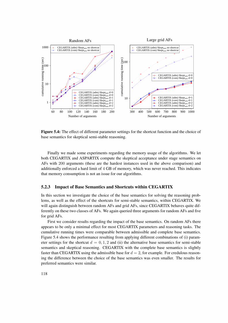
Random AFs

Number of arguments

cum

ulat

ive

runn

ing

time

(sec

)

●

●

●

●

●

●

●

●

●

1

10

100

1000

60 80 100 120 140 160 180 200

CEGARTIX (adm) Skeptsem no shortcutCEGARTIX (com) Skeptsem no shortcut

●

CEGARTIX (adm) Skeptsem d=0CEGARTIX (com) Skeptsem d=0CEGARTIX (adm) Skeptsem d=1CEGARTIX (com) Skeptsem d=1CEGARTIX (adm) Skeptsem d=2CEGARTIX (com) Skeptsem d=2

Large grid AFs

Number of arguments

cum

ulat

ive

runn

ing

time

(sec

)

●

●

●

●●

●

●

●

10

100

300 400 500 600 700 800 900 1000

CEGARTIX (adm) Skeptsem no shortcutCEGARTIX (com) Skeptsem no shortcut

CEGARTIX (adm) Skeptsem d=0CEGARTIX (com) Skeptsem d=0

● CEGARTIX (adm) Skeptsem d=1CEGARTIX (com) Skeptsem d=1CEGARTIX (adm) Skeptsem d=2CEGARTIX (com) Skeptsem d=2

Figure 5.4: The effect of different parameter settings for the shortcut function and the choice ofbase semantics for skeptical semi-stable reasoning.

Finally we made some experiments regarding the memory usage of the algorithms. We letboth CEGARTIX and ASPARTIX compute the skeptical acceptance under stage semantics onAFs with 200 arguments (these are the hardest instances used in the above comparison) andadditionally enforced a hard limit of 4 GB of memory, which was never reached. This indicatesthat memory consumption is not an issue for our algorithms.

5.2.3 Impact of Base Semantics and Shortcuts within CEGARTIX

In this section we investigate the choice of the base semantics for solving the reasoning prob-lems, as well as the effect of the shortcuts for semi-stable semantics, within CEGARTIX. Wewill again distinguish between random AFs and grid AFs, since CEGARTIX behaves quite dif-ferently on these two classes of AFs. We again queried three arguments for random AFs and fivefor grid AFs.

First we consider results regarding the impact of the base semantics. On random AFs thereappears to be only a minimal effect for most CEGARTIX parameters and reasoning tasks. Thecumulative running times were comparable between admissible and complete base semantics.Figure 5.4 shows the performance resulting from applying different combinations of (i) param-eter settings for the shortcut d = 0, 1, 2 and (ii) the alternative base semantics for semi-stablesemantics and skeptical reasoning. CEGARTIX with the complete base semantics is slightlyfaster than CEGARTIX using the admissible base for d = 2, for example. For credulous reason-ing the difference between the choice of the base semantics was even smaller. The results forpreferred semantics were similar.

118

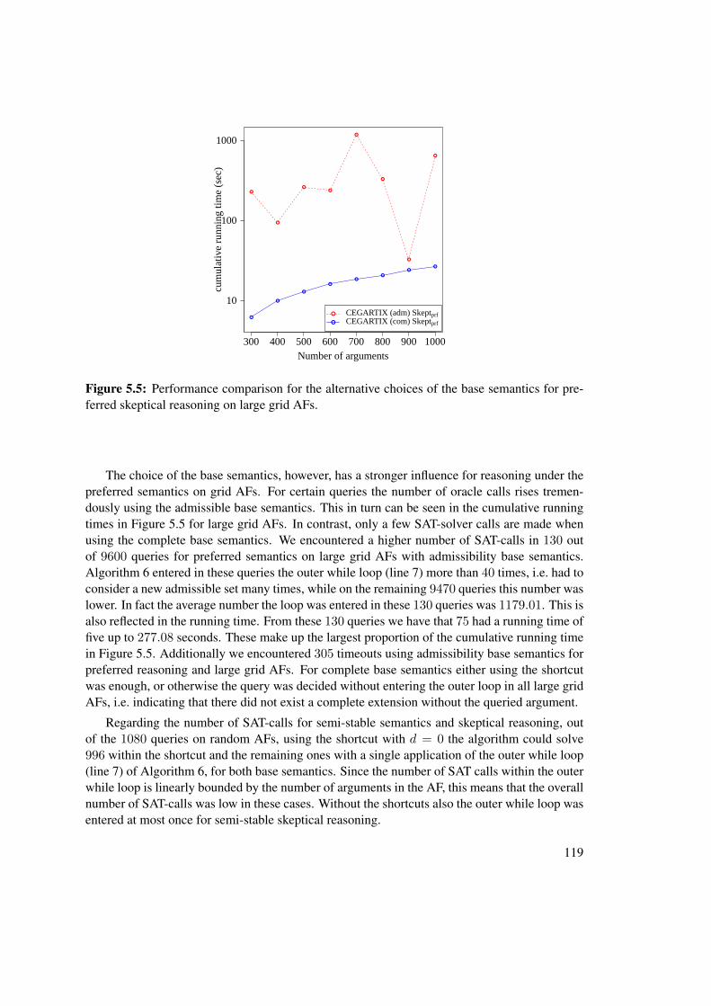
Number of arguments

cum

ulat

ive

runn

ing

time

(sec

)

●

●

●●

●

●

●

●

●

●

●

●

●●

●●

10

100

1000

300 400 500 600 700 800 900 1000

●

●

CEGARTIX (adm) SkeptprfCEGARTIX (com) Skeptprf

Figure 5.5: Performance comparison for the alternative choices of the base semantics for pre-ferred skeptical reasoning on large grid AFs.

The choice of the base semantics, however, has a stronger influence for reasoning under thepreferred semantics on grid AFs. For certain queries the number of oracle calls rises tremen-dously using the admissible base semantics. This in turn can be seen in the cumulative runningtimes in Figure 5.5 for large grid AFs. In contrast, only a few SAT-solver calls are made whenusing the complete base semantics. We encountered a higher number of SAT-calls in 130 outof 9600 queries for preferred semantics on large grid AFs with admissibility base semantics.Algorithm 6 entered in these queries the outer while loop (line 7) more than 40 times, i.e. had toconsider a new admissible set many times, while on the remaining 9470 queries this number waslower. In fact the average number the loop was entered in these 130 queries was 1179.01. This isalso reflected in the running time. From these 130 queries we have that 75 had a running time offive up to 277.08 seconds. These make up the largest proportion of the cumulative running timein Figure 5.5. Additionally we encountered 305 timeouts using admissibility base semantics forpreferred reasoning and large grid AFs. For complete base semantics either using the shortcutwas enough, or otherwise the query was decided without entering the outer loop in all large gridAFs, i.e. indicating that there did not exist a complete extension without the queried argument.

Regarding the number of SAT-calls for semi-stable semantics and skeptical reasoning, outof the 1080 queries on random AFs, using the shortcut with d = 0 the algorithm could solve996 within the shortcut and the remaining ones with a single application of the outer while loop(line 7) of Algorithm 6, for both base semantics. Since the number of SAT calls within the outerwhile loop is linearly bounded by the number of arguments in the AF, this means that the overallnumber of SAT-calls was low in these cases. Without the shortcuts also the outer while loop wasentered at most once for semi-stable skeptical reasoning.

119

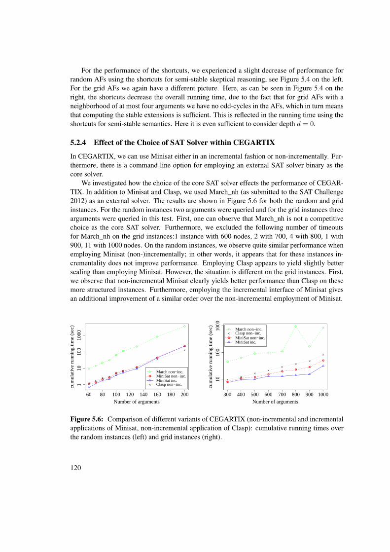
For the performance of the shortcuts, we experienced a slight decrease of performance forrandom AFs using the shortcuts for semi-stable skeptical reasoning, see Figure 5.4 on the left.For the grid AFs we again have a different picture. Here, as can be seen in Figure 5.4 on theright, the shortcuts decrease the overall running time, due to the fact that for grid AFs with aneighborhood of at most four arguments we have no odd-cycles in the AFs, which in turn meansthat computing the stable extensions is sufficient. This is reflected in the running time using theshortcuts for semi-stable semantics. Here it is even sufficient to consider depth d = 0.

5.2.4 Effect of the Choice of SAT Solver within CEGARTIX

In CEGARTIX, we can use Minisat either in an incremental fashion or non-incrementally. Fur-thermore, there is a command line option for employing an external SAT solver binary as thecore solver.

We investigated how the choice of the core SAT solver effects the performance of CEGAR-TIX. In addition to Minisat and Clasp, we used March_nh (as submitted to the SAT Challenge2012) as an external solver. The results are shown in Figure 5.6 for both the random and gridinstances. For the random instances two arguments were queried and for the grid instances threearguments were queried in this test. First, one can observe that March_nh is not a competitivechoice as the core SAT solver. Furthermore, we excluded the following number of timeoutsfor March_nh on the grid instances:1 instance with 600 nodes, 2 with 700, 4 with 800, 1 with900, 11 with 1000 nodes. On the random instances, we observe quite similar performance whenemploying Minisat (non-)incrementally; in other words, it appears that for these instances in-crementality does not improve performance. Employing Clasp appears to yield slightly betterscaling than employing Minisat. However, the situation is different on the grid instances. First,we observe that non-incremental Minisat clearly yields better performance than Clasp on thesemore structured instances. Furthermore, employing the incremental interface of Minisat givesan additional improvement of a similar order over the non-incremental employment of Minisat.

Number of arguments

cum

ulat

ive

runn

ing

time

(sec

)

●●

●●

●●

●

●

●

110

100

1000

60 80 100 120 140 160 180 200

●

March non−inc.MiniSat non−inc.MiniSat inc.Clasp non−inc.

Number of arguments

cum

ulat

ive

runn

ing

time

(sec

)

●

●●

●

●●

●

●

1010

010

00

300 400 500 600 700 800 900 1000

●

March non−inc.Clasp non−inc.MiniSat non−inc.MiniSat inc.

Figure 5.6: Comparison of different variants of CEGARTIX (non-incremental and incrementalapplications of Minisat, non-incremental application of Clasp): cumulative running times overthe random instances (left) and grid instances (right).

120

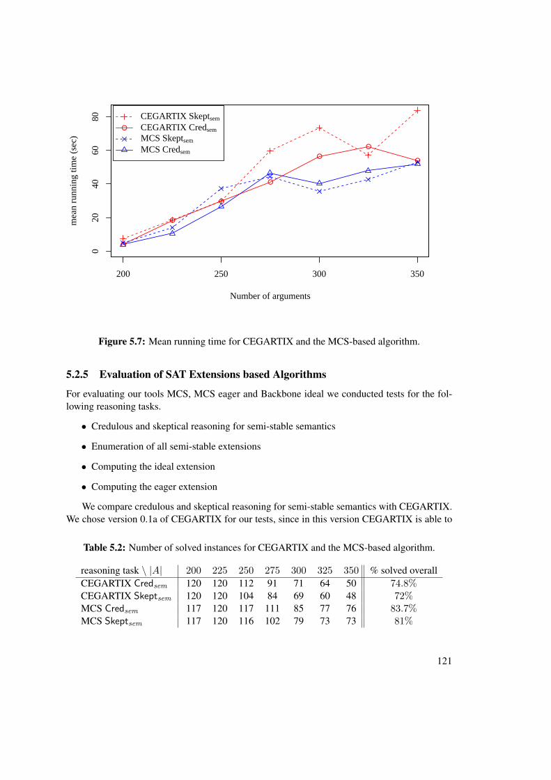
200 250 300 350

020

4060

80

Number of arguments

mea

n ru

nnin

g tim

e (s

ec)

●

●

●

●

●

●

●

●

CEGARTIX Skeptsem

CEGARTIX Credsem

MCS Skeptsem

MCS Credsem

Figure 5.7: Mean running time for CEGARTIX and the MCS-based algorithm.

5.2.5 Evaluation of SAT Extensions based Algorithms

For evaluating our tools MCS, MCS eager and Backbone ideal we conducted tests for the fol-lowing reasoning tasks.

• Credulous and skeptical reasoning for semi-stable semantics

• Enumeration of all semi-stable extensions

• Computing the ideal extension

• Computing the eager extension

We compare credulous and skeptical reasoning for semi-stable semantics with CEGARTIX.We chose version 0.1a of CEGARTIX for our tests, since in this version CEGARTIX is able to

Table 5.2: Number of solved instances for CEGARTIX and the MCS-based algorithm.

reasoning task \ |A| 200 225 250 275 300 325 350 % solved overallCEGARTIX Credsem 120 120 112 91 71 64 50 74.8%CEGARTIX Skeptsem 120 120 104 84 69 60 48 72%MCS Credsem 117 120 117 111 85 77 76 83.7%MCS Skeptsem 117 120 116 102 79 73 73 81%

121

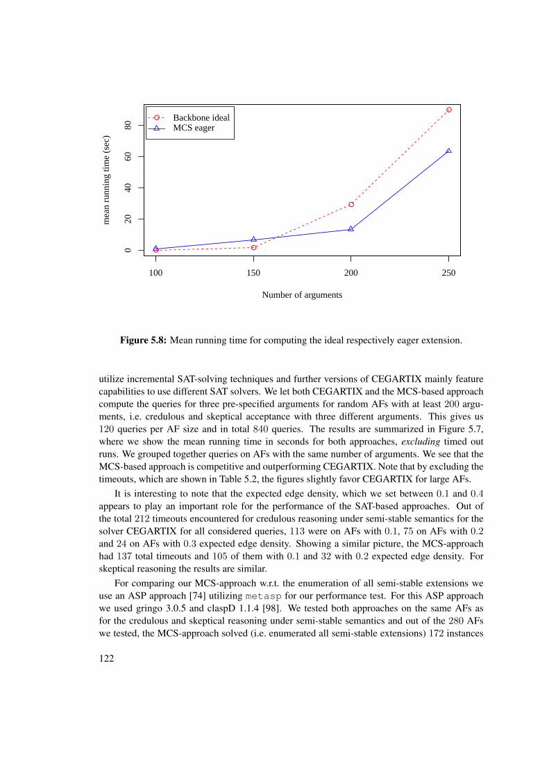
100 150 200 250

020

4060

80

Number of arguments

mea

n ru

nnin

g tim

e (s

ec)

● ●

●

●

● Backbone idealMCS eager

Figure 5.8: Mean running time for computing the ideal respectively eager extension.

utilize incremental SAT-solving techniques and further versions of CEGARTIX mainly featurecapabilities to use different SAT solvers. We let both CEGARTIX and the MCS-based approachcompute the queries for three pre-specified arguments for random AFs with at least 200 argu-ments, i.e. credulous and skeptical acceptance with three different arguments. This gives us120 queries per AF size and in total 840 queries. The results are summarized in Figure 5.7,where we show the mean running time in seconds for both approaches, excluding timed outruns. We grouped together queries on AFs with the same number of arguments. We see that theMCS-based approach is competitive and outperforming CEGARTIX. Note that by excluding thetimeouts, which are shown in Table 5.2, the figures slightly favor CEGARTIX for large AFs.

It is interesting to note that the expected edge density, which we set between 0.1 and 0.4appears to play an important role for the performance of the SAT-based approaches. Out ofthe total 212 timeouts encountered for credulous reasoning under semi-stable semantics for thesolver CEGARTIX for all considered queries, 113 were on AFs with 0.1, 75 on AFs with 0.2and 24 on AFs with 0.3 expected edge density. Showing a similar picture, the MCS-approachhad 137 total timeouts and 105 of them with 0.1 and 32 with 0.2 expected edge density. Forskeptical reasoning the results are similar.

For comparing our MCS-approach w.r.t. the enumeration of all semi-stable extensions weuse an ASP approach [74] utilizing metasp for our performance test. For this ASP approachwe used gringo 3.0.5 and claspD 1.1.4 [98]. We tested both approaches on the same AFs asfor the credulous and skeptical reasoning under semi-stable semantics and out of the 280 AFswe tested, the MCS-approach solved (i.e. enumerated all semi-stable extensions) 172 instances

122

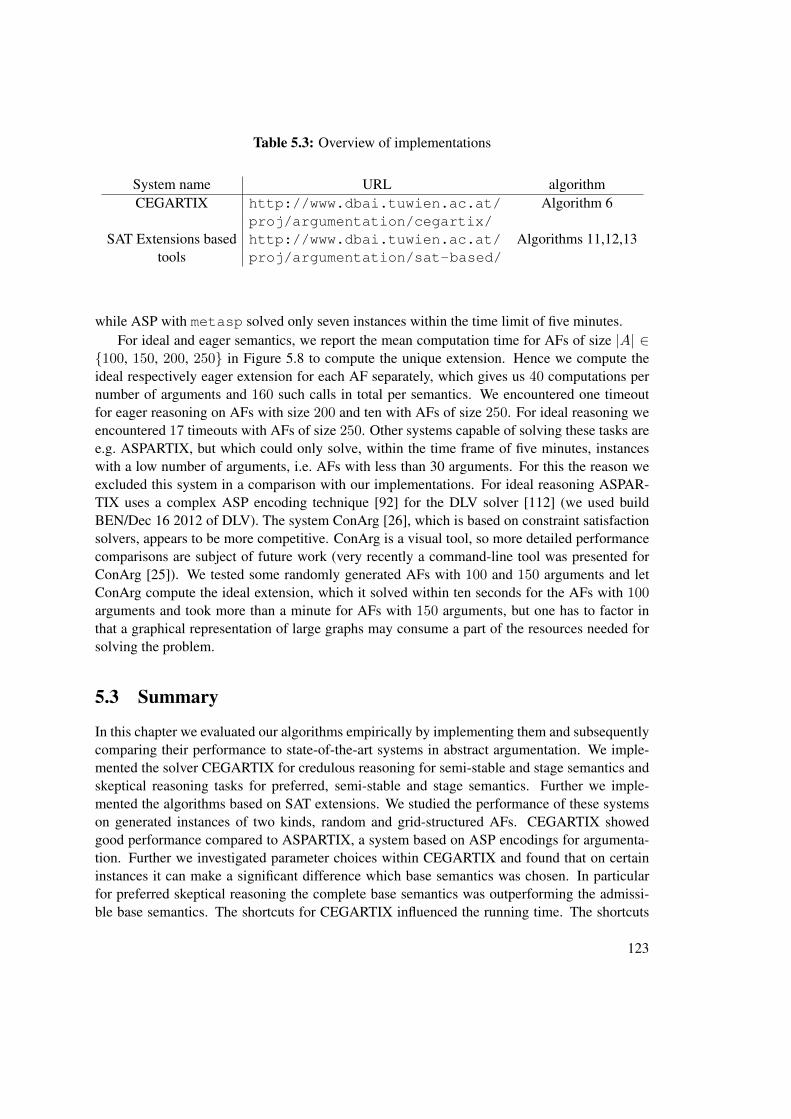
Table 5.3: Overview of implementations

System name URL algorithmCEGARTIX http://www.dbai.tuwien.ac.at/

proj/argumentation/cegartix/Algorithm 6

SAT Extensions based http://www.dbai.tuwien.ac.at/proj/argumentation/sat-based/

Algorithms 11,12,13tools

while ASP with metasp solved only seven instances within the time limit of five minutes.For ideal and eager semantics, we report the mean computation time for AFs of size |A| ∈

{100, 150, 200, 250} in Figure 5.8 to compute the unique extension. Hence we compute theideal respectively eager extension for each AF separately, which gives us 40 computations pernumber of arguments and 160 such calls in total per semantics. We encountered one timeoutfor eager reasoning on AFs with size 200 and ten with AFs of size 250. For ideal reasoning weencountered 17 timeouts with AFs of size 250. Other systems capable of solving these tasks aree.g. ASPARTIX, but which could only solve, within the time frame of five minutes, instanceswith a low number of arguments, i.e. AFs with less than 30 arguments. For this the reason weexcluded this system in a comparison with our implementations. For ideal reasoning ASPAR-TIX uses a complex ASP encoding technique [92] for the DLV solver [112] (we used buildBEN/Dec 16 2012 of DLV). The system ConArg [26], which is based on constraint satisfactionsolvers, appears to be more competitive. ConArg is a visual tool, so more detailed performancecomparisons are subject of future work (very recently a command-line tool was presented forConArg [25]). We tested some randomly generated AFs with 100 and 150 arguments and letConArg compute the ideal extension, which it solved within ten seconds for the AFs with 100arguments and took more than a minute for AFs with 150 arguments, but one has to factor inthat a graphical representation of large graphs may consume a part of the resources needed forsolving the problem.

5.3 Summary

In this chapter we evaluated our algorithms empirically by implementing them and subsequentlycomparing their performance to state-of-the-art systems in abstract argumentation. We imple-mented the solver CEGARTIX for credulous reasoning for semi-stable and stage semantics andskeptical reasoning tasks for preferred, semi-stable and stage semantics. Further we imple-mented the algorithms based on SAT extensions. We studied the performance of these systemson generated instances of two kinds, random and grid-structured AFs. CEGARTIX showedgood performance compared to ASPARTIX, a system based on ASP encodings for argumenta-tion. Further we investigated parameter choices within CEGARTIX and found that on certaininstances it can make a significant difference which base semantics was chosen. In particularfor preferred skeptical reasoning the complete base semantics was outperforming the admissi-ble base semantics. The shortcuts for CEGARTIX influenced the running time. The shortcuts

123

http://www.dbai.tuwien.ac.at/proj/argumentation/cegartix/

http://www.dbai.tuwien.ac.at/proj/argumentation/cegartix/

http://www.dbai.tuwien.ac.at/proj/argumentation/sat-based/

http://www.dbai.tuwien.ac.at/proj/argumentation/sat-based/

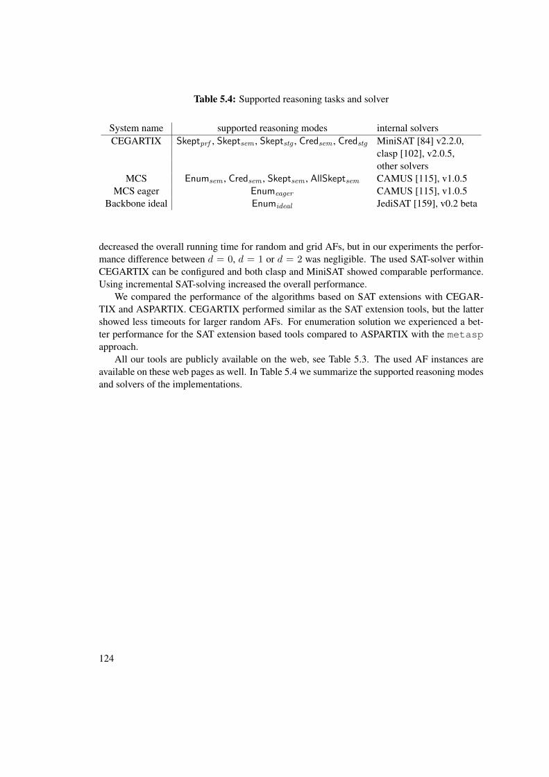
Table 5.4: Supported reasoning tasks and solver

System name supported reasoning modes internal solversCEGARTIX Skeptprf , Skeptsem , Skeptstg , Credsem , Credstg MiniSAT [84] v2.2.0,

clasp [102], v2.0.5,other solvers

MCS Enumsem , Credsem , Skeptsem , AllSkeptsem CAMUS [115], v1.0.5MCS eager Enumeager CAMUS [115], v1.0.5

Backbone ideal Enumideal JediSAT [159], v0.2 beta

decreased the overall running time for random and grid AFs, but in our experiments the perfor-mance difference between d = 0, d = 1 or d = 2 was negligible. The used SAT-solver withinCEGARTIX can be configured and both clasp and MiniSAT showed comparable performance.Using incremental SAT-solving increased the overall performance.

We compared the performance of the algorithms based on SAT extensions with CEGAR-TIX and ASPARTIX. CEGARTIX performed similar as the SAT extension tools, but the lattershowed less timeouts for larger random AFs. For enumeration solution we experienced a bet-ter performance for the SAT extension based tools compared to ASPARTIX with the metaspapproach.

All our tools are publicly available on the web, see Table 5.3. The used AF instances areavailable on these web pages as well. In Table 5.4 we summarize the supported reasoning modesand solvers of the implementations.

124

CHAPTER 6Discussion

In this chapter we recapitulate our contributions, point to important related work and give direc-tions for future research.

6.1 Summary

In this thesis we developed novel algorithms for two formalisms in abstract argumentation,Dung’s argumentation frameworks (AFs) and the more recent abstract dialectical frameworks(ADFs). We provided algorithms for solving credulous and skeptical acceptance of an argumentin an AF, as well as for enumeration of all extensions. The algorithms are capable of solvingthese tasks for the preferred, semi-stable, stage, ideal, eager and stage-ideal semantics. Furtherwe showed how to generalize the algorithms to work with ADFs for preferred and groundedsemantics.

Many existing approaches for algorithms in abstract argumentation can be classified into ei-ther direct approaches or reduction based approaches. The former aims at building a dedicatedprocedure from scratch, typically exploiting domain specific knowledge for increasing the over-all performance. The idea of the latter approach is to encode the problem at hand into anotherusually declarative language, for which sophisticated solvers exist. Many existing reductionbased approaches are monolithic in the sense that a single encoding is constructed for the prob-lem at hand. One of the main benefits of reduction approaches is that they may re-use softwareand can often be instantiated faster than direct approaches. We choose the best of the two worldsof direct and reduction approaches and developed a hybrid variant. We delegate certain complexsubtasks to search engines, but hereby do not translate the whole problem in one monolithicencoding.

The problems we solve in this thesis are all “beyond” NP, i.e. hardness was shown for almostall considered tasks for a class above NP. A purely monolithic efficient reduction approachrequires search engines matching the complexity of the problem to solve. In contrast, our novelalgorithms iteratively call engines to compute subtasks, which are less complex than the overall

125

task. We showed that the number of required calls in the worst case is related to two inherentparameters of the given AF/ADF. This means if these parameters are low, then so is the numberof required calls.

We classified our algorithms into two categories:

• search algorithms; and

• algorithms utilizing SAT extensions.

We showed that both approaches can solve numerous reasoning tasks for AFs and ADFs.The basic idea of the search algorithms to compute a reasoning task for a semantics σ is to fallback to a simpler semantics σ′, called the base semantics. From this base semantics we requirethat its maximal elements w.r.t. a preorder are exactly those in σ. Now we let the solvers com-pute candidates from the base semantics and then iteratively maximize them to find a maximalcandidate in σ. Using this approach we can solve tasks for enumerating all solutions or decidecredulous or skeptical acceptance of σ for an argument a. For AFs we applied search algorithmsfor preferred, semi-stable and stage semantics and for ADFs we applied them to preferred se-mantics.

We considered two SAT extensions in our work, the minimal correction sets (MCSes) andbackbones. We derived algorithms based on MCSes in a very natural way for the semi-stable andstage semantics. Using a simple post processor we showed how to find the eager extension andthe stage-ideal extension. For the ideal semantics we instantiated an existing algorithm usingbackbones.

Existing algorithms for computing MCSes and backbones from the SAT community rely oniterative SAT solving. We slightly adapted an algorithm for MCSes and directly used an algo-rithm for backbones for our purposes. For the computation of subtasks for our search algorithms,we can, for AFs, in all cases use a SAT-solver, since the corresponding decision problems arein NP or in coNP. For ADFs the picture is different. Here we first had to establish a clear the-oretical understanding of the computational complexity which was missing in the literature foralmost all considered problems. The result of this analysis is that the reasoning tasks for ADFsare “one step up” in the polynomial hierarchy compared to their counterparts on AFs. Thisdirectly implies that our search algorithms, under standard complexity theoretic assumptions,cannot be instantiated with a SAT-solver, unless we take an exponential blow-up into account.However we can use solvers capable of solving tasks of the second level of the polynomial hi-erarchy (e.g. solving tasks which are in ΣP

2 ). Examples of such solvers are quantified Booleanformulae (QBF) solvers or answer-set programming (ASP) solvers capable of dealing with dis-junctive ASP programs. As a side result from our complexity analysis we developed a backbonealgorithm for computing the grounded interpretation of an ADF.

A second major contribution of our complexity analysis is the investigation of BADFs withknown link types. Here we proved that the reasoning tasks on these BADFs have the samecomplexity as their counterparts on AFs. This clearly suggests to use again less powerful solversfor BADFs such as SAT-solvers or ASP solvers (and normal logic programs).

To show the feasibility of our approach we conducted experiments on prototypical imple-mentations of our algorithms for AFs. The experiments revealed a significant performance boost

126

compared to ASPARTIX, a state-of-the-art system for computing many semantics for AFs. CE-GARTIX is our prototype for instantiating the search algorithms. For the algorithms based onSAT extension, we provide a suite of tools. All programs are available online (see Table 5.3).

6.2 Related Work

Naturally no academic work exists purely in a vacuum. In this section we describe the mostimportant related works to our thesis. Algorithms applicable for problems in abstract argumen-tation are discussed in a recent survey [47]. As mentioned earlier one can distinguish betweenreduction-based and direct approaches. The former aim at translating a given problem to an-other, usually well-studied problem, for which efficient search engines are available. The goalof the latter approach is to directly develop algorithms tailored to the given problem domain. Wereview the most important related work in this regard and give further pointers to the literature.Subsequently we discuss algorithms based on decompositions of the given AF and conclude thissection with further related work.

Reduction based Approaches The main directions for reduction based approaches for ab-stract argumentation feature SAT, QBFs, answer-set programming (ASP), constraint satisfactionproblems (CSP) and equational systems. As a common feature all these formalisms specifysome form of constraints to be satisfied. By carefully choosing the right constraints one canthen implement the problems from abstract argumentation in these formalisms. We highlightparticularly important related work.

The most well-known system is probably ASPARTIX [74, 85, 92], a reduction-based ap-proach with ASP as the target language. This system features an easy-to-use interface. One sim-ply has to provide a text file with the AF as input in a very simple language. Our systems supportthis language as well (see Section 5.1). This format is sometimes also called ASPARTIX format.Many systems in abstract argumentation are compared with ASPARTIX [25, 45, 74, 129, 131].Other ASP based approaches have been collected in a recent overview paper [148].

Another approach using CSP [26] is ConArg. This system is capable of computing manysemantics and features a GUI. Reductions to equational systems have been studied in [96].

Related work in the SAT area is, for obvious reasons, very close to our work. The mostfundamental work is by Besnard and Doutre in [21], who encoded several AF semantics inBoolean formulae, such that the extensions and models correspond. Many of their encodings, orin cases key ideas of their encodings, are visible in more recent approaches. We also partiallyuse their encodings. Although [21] provided also encodings for preferred extensions, it is clearfrom the computational complexity point of view that we require for this to work more powerfulengines than SAT-solvers. In [2, 86] several problems for AFs were reduced to encodings forQBFs.

The most relevant SAT based approach is PrefSat by Cerutti et al. [45], which enumeratesall preferred labelings. In contrast to other SAT based systems, this is not a monolithic reductionapproach. This means that not a single encoding is constructed, which has as its solutions exactlythe answer to the original problem, but multiple calls to a SAT-solver are applied. Indeed theoverall scheme is similar to our search algorithms. The key difference lies actually in the use

127

of labelings instead of extensions in the Boolean encodings. Unlike CEGARTIX, the resultingsystem of their work enumerates all preferred labelings.

PrefSat encodes labelings of an AF F = (A = (x1, . . . , xn), R) by generating three vari-ables per argument, i.e. the set of variables in the constructed formula are {Ii, Oi, Ui | 1 ≤i ≤ |A|}. These then correspond in the final result naturally to a labeling. This means a three-valued labeling J corresponds to a model K if J = (I,O, U) with I = {Ii | K(Ii) = t},O = {Oi | K(Oi) = t} and U = {Ui | K(Ui) = t}. Encoding the basic constraint that forevery argument exactly one labeling is assigned can be done as follows.∧

1≤i≤|A|

((Ii ∨Oi ∨ Ui) ∧ (¬Ii ∨Oi) ∧ (¬Ii ∨ ¬Ui) ∧ (¬Oi ∨ Ui)

)Then one can encode the conditions for a labeling to be complete (see Definition 2.3.11) by

conjoining certain subformulae. For instance the formula∧1≤i≤|A|,∃(y,xi)∈R

( ∧(xj ,xi)∈R

(¬Ii ∨Oj))

encodes that if there is an attacker for the argument xi, then one creates a clause for each suchattacker xj such that if xi is assigned the labeling in (Ii is true), then xj must necessarilybe out (Oj is true). One can encode the other conditions as well in Boolean logic. Severalequivalent formulae for doing this have been investigated by Cerutti et al. [45]. In our encodingfor complete extensions (see Lemma 3.3.7 and Proposition 3.3.8) we can infer a labeling of anargument x via the value it is assigned in a model and its “range” variable x. If x is false in themodel, then x is undecided. Otherwise if x is true and x is false, then x is out. If x is true in themodel, then x is in. The labelings/extensions can be directly computed with both our and theirencoding. Comparing these encodings w.r.t. their performance is subject to future work.

The idea of the iterative SAT algorithm PrefSat is very close to our Algorithm 3. The basicmethodology is to iteratively find complete labelings and extend them to preferred labelings byiterative calls to a SAT-solver. If such a preferred labeling is found, one excludes it from futureiterations and searches for a fresh candidate. At the end all preferred labelings are enumerated.

The system PrefSat from [45] is capable of using two state-of-the-art SAT-solvers, PrecoSAT(from the 2009 SAT competition) and Glucose [5]. PrefSat was compared with ASPARTIX [85](also using metasp, see [74]) and the system presented in [131]. In the experiments the itera-tive SAT approach outperformed the other systems. We view the results of Cerutti et al. as anindependent development with many similarities to our approach. Their performance analysisdraws a similar conclusion than ours, namely that the iterative SAT scheme performs very wellcompared to monolithic systems. Thus our results and theirs complement each other and showthat the overall idea behind our approaches is beneficial for implementing hard problems arisingin abstract argumentation.

Direct Algorithms for Abstract Argumentation Direct approaches include labeling-basedapproaches [38] and game-theoretic approaches [126]. For labeling based approaches severalprocedures have been published [57, 126, 129, 130, 131, 152]. Central for these algorithms isthat if one fixes a label of some argument, then for complete labelings one can propagate the

128

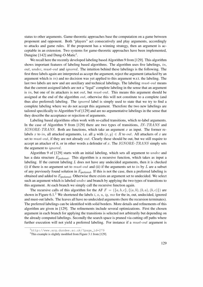
status to other arguments. Game-theoretic approaches base the computation on a game betweenproponent and opponent. Both “players” act consecutively and play arguments, accordinglyto attacks and game rules. If the proponent has a winning strategy, then an argument is ac-ceptable in an extension. Two systems for game-theoretic approaches have been implemented,Dungine [142] and Dung-O-Matic1.

We recall here the recently developed labeling based Algorithm 9 from [129]. This algorithmshows important features of labeling based algorithms. The algorithm uses five labelings, in,out, undec, must-out and ignored . The intuition behind these labelings is the following. Thefirst three labels again are interpreted as accept the argument, reject the argument (attacked by anargument which is in) and no decision was yet applied to this argument w.r.t. the labeling. Thelast two labels are new and are auxiliary and technical labelings. The labeling must-out meansthat the current assigned labels are not a “legal” complete labeling in the sense that an argumentis in, but one of its attackers is not out, but must-out . This means this argument should beassigned at the end of the algorithm out, otherwise this will not constitute to a complete (andthus also preferred) labeling. The ignored label is simply used to state that we try to find acomplete labeling where we do not accept this argument. Therefore the two new labelings aretailored specifically to Algorithm 9 of [129] and are no argumentative labelings in the sense thatthey describe the acceptance or rejection of arguments.

Labeling based algorithms often work with so-called transitions, which re-label arguments.In the case of Algorithm 9 from [129] there are two types of transitions, IN -TRANS andIGNORE -TRANS . Both are functions, which take an argument x as input. The former re-labels x to in, all attacked arguments, i.e. all y with (x, y) ∈ R to out. All attackers of x areset to must-out , if they are not already out. Clearly these should be out, but we still require toaccept an attacker of it, or in other words a defender of x. The IGNORE -TRANS simply setsthe argument to ignored .

Algorithm 9 of [129] starts with an initial labeling, which sets all argument to undec andhas a data structure Epreferred. This algorithm is a recursive function, which takes as input alabeling. If the current labeling L does not have any undecided arguments, then it is checked(i) if there is no argument set to must-out and (ii) if the arguments set to in by L are a subsetof any previously found solution in Epreferred. If this is not the case, then a preferred labeling isobtained and added to Epreferred. Otherwise there exists an argument set to undecided. We selectsuch an argument which is labeled undec and branch by applying the two types of transitions tothis argument. At each branch we simply call the recursive function again.

The recursive calls of this algorithm for the AF F = ({a, b, c}, {(a, b), (b, a), (b, c)}) areshown in Figure 6.1.2 We shortened the labels i, o, u, ig , mo for the in, out, undecided, ignoredand must-out labels. The leaves all have no undecided arguments (here the recursion terminates).The preferred labelings can be identified with solid borders. More details and refinements of thisalgorithm are given in [129]. The refinements include several optimizations. First the chosenargument in each branch for applying the transitions is selected not arbitrarily but depending onthe already computed labelings. Secondly the search space is pruned via cutting off paths wherefurther execution will not yield a preferred labeling. For instance if a must-out argument is

1http://www.arg.dundee.ac.uk/?page_id=2792This example is slightly modified from Figure 3.1 from [129].

129

http://www.arg.dundee.ac.uk/?page_id=279

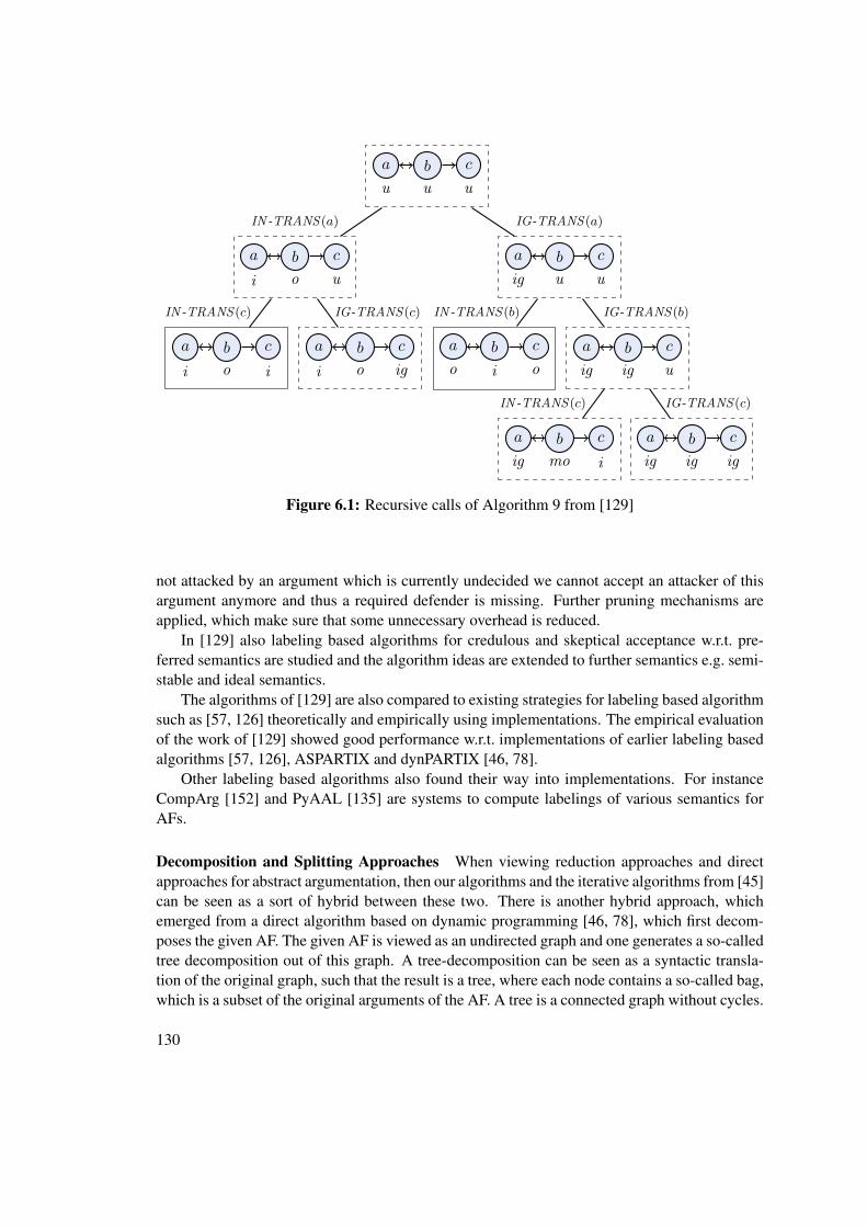
a

u

b

u

c

u

a

i

b

o

c

u

a

ig

b

u

c

u

a

i

b

o

c

i

a

i

b

o

c

ig

a

o

b

i

c

o

a

ig

b

ig

c

u

a

ig

b

mo

c

i

a

ig

b

ig

c

ig

IN -TRANS(a) IG-TRANS(a)

IN -TRANS(c) IG-TRANS(c) IN -TRANS(b) IG-TRANS(b)

IN -TRANS(c) IG-TRANS(c)

Figure 6.1: Recursive calls of Algorithm 9 from [129]

not attacked by an argument which is currently undecided we cannot accept an attacker of thisargument anymore and thus a required defender is missing. Further pruning mechanisms areapplied, which make sure that some unnecessary overhead is reduced.

In [129] also labeling based algorithms for credulous and skeptical acceptance w.r.t. pre-ferred semantics are studied and the algorithm ideas are extended to further semantics e.g. semi-stable and ideal semantics.

The algorithms of [129] are also compared to existing strategies for labeling based algorithmsuch as [57, 126] theoretically and empirically using implementations. The empirical evaluationof the work of [129] showed good performance w.r.t. implementations of earlier labeling basedalgorithms [57, 126], ASPARTIX and dynPARTIX [46, 78].

Other labeling based algorithms also found their way into implementations. For instanceCompArg [152] and PyAAL [135] are systems to compute labelings of various semantics forAFs.

Decomposition and Splitting Approaches When viewing reduction approaches and directapproaches for abstract argumentation, then our algorithms and the iterative algorithms from [45]can be seen as a sort of hybrid between these two. There is another hybrid approach, whichemerged from a direct algorithm based on dynamic programming [46, 78], which first decom-poses the given AF. The given AF is viewed as an undirected graph and one generates a so-calledtree decomposition out of this graph. A tree-decomposition can be seen as a syntactic transla-tion of the original graph, such that the result is a tree, where each node contains a so-called bag,which is a subset of the original arguments of the AF. A tree is a connected graph without cycles.

130

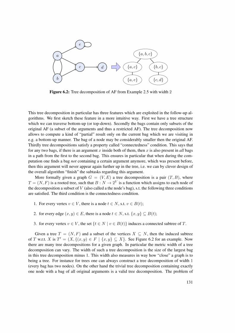
a

b

c d

e

{a, c}

{a, e}

{a, b, c}

{b, c}

{c, d}

Figure 6.2: Tree decomposition of AF from Example 2.5 with width 2

This tree decomposition in particular has three features which are exploited in the follow-up al-gorithms. We first sketch these feature in a more intuitive way. First we have a tree structurewhich we can traverse bottom-up (or top-down). Secondly the bags contain only subsets of theoriginal AF (a subset of the arguments and thus a restricted AF). The tree decomposition nowallows to compute a kind of “partial” result only on the current bag which we are visiting ine.g. a bottom-up manner. The bag of a node may be considerably smaller then the original AF.Thirdly tree decompositions satisfy a property called “connectedness” condition. This says thatfor any two bags, if there is an argument x inside both of them, then x is also present in all bagsin a path from the first to the second bag. This ensures in particular that when during the com-putation one finds a bag not containing a certain argument anymore, which was present before,then this argument will never appear again further up in the tree, i.e. we can by clever design ofthe overall algorithm “finish” the subtasks regarding this argument.

More formally given a graph G = (V,E) a tree decomposition is a pair (T,B), whereT = (N,F ) is a rooted tree, such that B : N → 2V is a function which assigns to each node ofthe decomposition a subset of V (also called a the node’s bag), s.t. the following three conditionsare satisfied. The third condition is the connectedness condition.

1. For every vertex v ∈ V , there is a node t ∈ N , s.t. v ∈ B(t);

2. for every edge (x, y) ∈ E, there is a node t ∈ N , s.t. {x, y} ⊆ B(t);

3. for every vertex v ∈ V , the set {t ∈ N | v ∈ B(t)} induces a connected subtree of T .

Given a tree T = (N,F ) and a subset of the vertices X ⊆ N , then the induced subtreeof T w.r.t. X is T ′ = (X, {(x, y) ∈ F | {x, y} ⊆ X}. See Figure 6.2 for an example. Nowthere are many tree decompositions for a given graph. In particular the metric width of a treedecomposition can vary. The width of such a tree decomposition is the size of the largest bagin this tree decomposition minus 1. This width also measures in way how “close” a graph is tobeing a tree. For instance for trees one can always construct a tree decomposition of width 1(every bag has two nodes). On the other hand the trivial tree decomposition containing exactlyone node with a bag of all original arguments is a valid tree decomposition. The problem of

131

finding an optimal tree decomposition w.r.t. width is intractable [3], but heuristics and softwareimplementations exists [128].

The approach from dynPARTIX [46, 78] now first computes a tree decomposition with apotentially low width. Then it traverses this tree decomposition in a bottom-up manner for thecomputation of preferred semantics. The concrete dynamic programming algorithm for enumer-ation of preferred extensions is somewhat technically involved. In essence so-called colorings ofthe arguments are computed in each bag, or sets of such colorings. Colorings are a data structureto hold information of the status of arguments computed so far. Then these colorings are prop-agated upwards and the new arguments from the next bag are considered. We refer the readerto [80] for details of the algorithm. A particularly important aspect of dynPARTIX is that theruntime depends on the treewidth of the decomposition.

In later works, the computation in each bag is delegated to an ASP solver in the frame-work of D-FLAT [27, 28]. First the given AF is decomposed to a tree decomposition. Then thebottom-up algorithm is applied using for each computation an ASP call. Comparing the dynamicprogramming approach using D-FLAT with our algorithms (e.g. Algorithm 1), we have in oursearch algorithms a sequence of calls to a SAT-solver for semantical (sub)problems. On the otherhand using dynPARTIX and D-FLAT one syntactically decomposes the given AF and then ap-plies a dynamic programming algorithm using ASP calls for restricted AFs. Furthermore, whenwe compare the inherent parameters used in the two approaches, then dynPARTIX and D-FLATutilize treewidth as the parameter, while we utilize semantical parameters. First experimentsfor dynPARTIX showed that if the structure of the given AF emits a tree decomposition of lowwidth, then the computation can be efficiently done.

Another related approach to the decomposition approach via tree decomposition is via split-ting [14, 15, 16]. The basic idea is to split an AF into two parts. We then have a left and rightpart. For all attackers from the right to the left side we attach to the restricted AF from the leftside auxiliary arguments, which attack those attacked arguments and back (symmetric attacks).Then the extensions are computed on this adapted framework from the left part. The auxiliaryarguments act as “gadgets” to simulate that we either may put them inside an extension or not.For each extension of the left part we adapt the right restricted framework by basically propa-gating the extension. For instance if an argument a is inside an extension E of the left part andin the original (whole) framework there is an attack (a, b) to an argument b of the right part, thenwe insert auxiliary arguments and attacks on the right framework for ensuring that b is not inthe extension. The concrete gadgets depend on the chosen semantics. We can then combine theextensions of the right part with the extension of the left part. In this way one can enumerate allextensions.

This idea was implemented and empirically evaluated in [16]. The results show that if theAF in question has certain characteristics, e.g. having a suitable SCC structure for splitting, thenthis approach increased the overall performance.

Other Related Systems and Algorithm Concepts An interesting approach for optimizingqueries for preferred semantics is studied in [114]. Here the idea is to first compute the groundedextension of an AF and then propagating the result. This may dramatically influence the runningtime. The preprocessing step can be computed in polynomial time and may cover the status of

132

many arguments. Further it was observed that if we want to check for credulous and skepticalacceptance of arguments w.r.t. the preferred semantics we can restrict the given AF only torelevant arguments for answering the query [113]. In particular one can look at the condensationof the given AF (its SCC graph, see Section 2.3.1). The condensation is a forest of rooted trees.Now it is sufficient for deciding the query to consider only those SCCs which have a path tothe one containing the argument under scrutiny. This in particular is based on the directionalityproperty of preferred semantics.

Regarding related work on algorithms for ADFs, there are two systems for ADFs. The firstis adfsys [91] and the other its successor DIAMOND [90]. Both are based on (disjunctive) ASPencodings. For more complex semantics more than one ASP call is applied or the input ADF isfirst preprocessed. This preprocessor maps a given ADF with Boolean formulae as acceptanceconditions into an ADF with functional representations. This representation essentially givesthe truth table of the formula, thus may be exponential in space w.r.t. the size of the ADF withformulae.

Another interesting approach for ADFs are translations of ADFs to AFs by Brewka, Dunneand Woltran [29] and Ellmauthaler [89]. Here translations for a fixed semantics of ADFs aregiven to a fixed semantics of AFs. They presented translations for computing ADF models viastable extensions of AFs. They also show that the stable semantics of ADFs, as defined in [34]can be translated to AFs. Such translations can also be used for analysing the complexity andfor providing algorithms.

Leaving the area of abstract argumentation there are two related works which we highlightdue to their similarities to our algorithms. The first one is an approach for the field of abduc-tion [134]. Briefly put in propositional abduction we are working with propositional formulaeand are given a knowledge base which contains our knowledge of the world. Then we havecertain observations or manifestations which we would like to have explained. Usually we aregiven a set of hypotheses, from which we may draw these explanations. The task is then to findcertain explanations of the manifestations which are consistent with our background knowledge.Typically one additionally applies certain constraints for these explanations, e.g. they shouldbe minimal w.r.t. the number of hypotheses used. Propositional abduction features problemscomplete for the second level of the polynomial hierarchy.

Pfandler, Rümmele and Szeider [134] proposed to use a so-called backdoor approach forabduction, which is based on parameterized complexity theory. Their approach encodes theproblem in a Boolean formula. In general this formula may be of exponential size w.r.t. theinput instance. However they show that this formula can be constructed in quadratic time witha constant factor that is exponential in a certain “distance” measure. This distance measuredescribes the distance of the given propositional theory in the abduction problem to the classesof Horn or Krom formulae. A clause is Horn if it has at most one positive literal and a clause isKrom if it has at most two literals. The satisfiability problem for formulae from these classes canbe decided in polynomial time. The distance is now measured in terms of the size of the smallestso-called strong backdoor set of the given theory to one of these classes. We define an auxiliaryconcept of simplifying a formula φ in CNF with a (partial) truth assignment γ, denoted as φ[γ]as follows. A clause c ∈ φ is in φ[γ] if atoms(c) ∩ dom(γ) = ∅. That is if the partial truthassignment does not set a variable of c to a value, then this clause c is present in φ[γ] unchanged.

133

If l ∈ c and γ(l) = t, then this clause is not in φ[γ]. If l ∈ c and γ(¬l) = t, then c′ = c \ {l} isin φ[γ]. No other clauses are present in φ[γ]. Briefly put, we remove all clauses already satisfiedby γ from φ. Additionally we remove all literals, which are evaluated to false from the clauses.Let C be a class of formulae in CNF. A strong C-backdoor set of a formula φ in CNF is a set ofvariables B, s.t. φ[γ] ∈ C for all possible truth assignments γ on the variables B. For instancea strong Krom-backdoor for the formula φ = (a ∨ b ∨ c) would be B = {a}. If a is set to truein a partial interpretation γ, then φ[γ] = >. Otherwise if γ(a) = f , then φ[γ] = (b ∨ c).

If we compare the approach of [134] to our algorithms, then the main difference is that in thebackdoor approach to abduction inherent parameters of the given instance determine the worstcase size of the resulting formula and in our algorithms parameters govern the worst case numberof calls to a SAT-solver, but all of the formulae in these calls can be constructed in polynomialtime.

Finally a related approach to our algorithms is the CEGAR (counter-example guided ab-straction refinement) approach [49, 50]. In our algorithms, we use the NP decision proceduresas NP oracles in an iterative fashion. Such approaches fall under the general CEGAR approachoriginating from the field of model checking. The CEGAR approach has been harnessed forsolving various other intrinsically hard reasoning problems [13, 55, 94, 105, 106, 107, 127, 141,155]. However, we are not aware of earlier work on developing CEGAR-based procedures,which are complexity-sensitive. In our algorithms if the AF in question is in a parameterizedclass of AFs which have milder complexity, then this implies a direct relation between the sizeof the AF, the parameter and the number of oracle calls.

6.3 Future Work

Optimizations and Extensions of Algorithms First of all our general scheme of search algo-rithms can be further extended to work with other semantics. In particular the novel SCC-basedstage2 [72] semantics appears intriguing. Since stage2 is based on the stage semantics an adap-tion of our search algorithm for stage semantics in an recursive SCC scheme seems to be aninteresting approach for the computationally complex stage2 semantics. Regarding SCCs ingeneral, as observed by [113] we can restrict ourselves to only relevant arguments for semanticssatisfying SCC-recursiveness [12] or directionality if we want to answer credulous or skepti-cal acceptance. It would be interesting to incorporate this optimization in our algorithms forpreferred semantics.

Further optimizations for AF algorithms include the realizability studies by Dunne et al. [65,66, 116]. They show which sets of extensions for a semantics σ are realizable, i.e. that one canconstruct an AF which has exactly the given set of sets as its σ-extensions. These kind of resultsmay be used to reduce the search space during running time of our algorithms. For instance ifwe currently have a certain set of preferred extensions already computed, then using realizabilityresults we may be able to conclude that certain kinds of extensions are not possible anymore andcan include corresponding constraints for pruning the search space. Furthermore the problemsobserved with complete base semantics for the Algorithm 6 may be explained more thoroughlyusing results from realizability.

134

Regarding algorithms for ADFs, we currently used only the admissible base semantics forpreferred semantics. Utilizing complete semantics for ADFs in the search algorithm may againlead to more efficient computation as we witnessed for AFs. Additionally we showed only howto generalize the search algorithms to preferred semantics. It would be interesting to see if othersemantics generalized from AFs, e.g. semi-stable semantics, can be captured within our generalsearch algorithm scheme.

Computational Complexity The complexity analysis of ADFs is still not finished. Recentlyan extension-based semantics for ADFs [136] was proposed. A detailed comparison of the novelextension-based semantics with the ADF semantics as defined in [31, 144] w.r.t. complexity iscurrently missing. Furthermore parametrized complexity, investigation of tractable fragmentsand backdoors [61, 79, 80, 81] are completely untouched topics for ADFs.

Implementations and Experimental Evaluation For concrete implementations we providedprograms using SAT-solvers. It would be interesting to see the difference if one uses other ora-cles such as CSP or ASP solvers instead of SAT-solvers. For ADFs our algorithms are currentlynot implemented and we may use QBF or disjunctive ASP solvers for general ADFs. For bipolarADFs we can use SAT-solvers or ASP solvers dealing with normal logic programs. For iterativeschemes it might also be interesting to try nested HEX programs [88], which offer nesting ofASP programs.

Currently there is a lack of benchmark suites for performance tests in argumentation [73].In particular AFs from applications are missing. Clearly this is highly desirable for future ex-perimentation.

General Future Work Abstract argumentation is embedded in a larger workflow. In the in-troduction we sketched this argumentation process (see Figure 1.1). Briefly put, we instantiatea framework out of a given knowledge base, compute sets of jointly acceptable arguments anddraw conclusions from them. For creating arguments several formal approaches have been stud-ied [103, 137]. For instance one can create arguments out of a knowledge bases consisting ofBoolean formulae or logical rules. In the argumentation process computing the status of abstractarguments is one intermediate step. Using knowledge from other steps of the workflow maydramatically increase the overall performance. In particular some framework structures mightnot be possible using certain instantiation schemes. Further it might be possible to augment e.g.an AF with further information from the original knowledge base and include this informationfor computing acceptability of arguments. Currently the steps are mostly viewed as independentchallenges and the process of combining knowledge from different steps is just in its infancy, butmight provide tremendous performance gains in solving problems for real world applications.

135

Bibliography

[1] Leila Amgoud and Henri Prade. Using Arguments for Making and Explaining Decisions.Artificial Intelligence, 173(3-4):413–436, 2009.

[2] Ofer Arieli and Martin W. A. Caminada. A QBF-Based Formalization of Abstract Argu-mentation Semantics. Journal of Applied Logic, 11(2):229–252, 2013.

[3] Stefan Arnborg, Derek G. Corneil, and Andrzej Proskurowski. Complexity of FindingEmbeddings in a k-tree. SIAM Journal of Algebraic Discrete Methods, 8:277–284, 1987.

[4] Roberto Asín, Robert Nieuwenhuis, Albert Oliveras, and Enric Rodríguez-Carbonell.Cardinality Networks: A Theoretical and Empirical Study. Constraints, 16(2):195–221,2011.

[5] Gilles Audemard and Laurent Simon. Predicting Learnt Clauses Quality in Modern SATSolvers. In Craig Boutilier, editor, Proceedings of the 21st International Joint Conferenceon Artificial Intelligence, IJCAI 2009, pages 399–404, 2009.

[6] Chitta Baral and Michael Gelfond. Logic Programming and Knowledge Representation.The Journal of Logic Programming, 19 & 20:73–148, 1994.

[7] Pietro Baroni, Martin W. A. Caminada, and Massimiliano Giacomin. An Introduction toArgumentation Semantics. The Knowledge Engineering Review, 26(4):365–410, 2011.

[8] Pietro Baroni and Massimiliano Giacomin. Evaluating Argumentation Semantics withRespect to Skepticism Adequacy. In Lluis Godo, editor, Proceedings of the Eight Eu-ropean Conference on Symbolic and Quantitative Approaches to Reasoning with Un-certainty, ECSQARU 2005, volume 3571 of Lecture Notes in Computer Science, pages329–340. Springer, 2005.

[9] Pietro Baroni and Massimiliano Giacomin. On Principle-Based Evaluation of Extension-Based Argumentation Semantics. Artificial Intelligence, 171(10-15):675–700, 2007.

[10] Pietro Baroni and Massimiliano Giacomin. A Systematic Classification of ArgumentationFrameworks where Semantics Agree. In Philippe Besnard, Sylvie Doutre, and AnthonyHunter, editors, Proceedings of the Second Conference on Computational Models of Argu-ment, COMMA 2008, volume 172 of Frontiers in Artificial Intelligence and Applications,pages 37–48. IOS Press, 2008.

137

[11] Pietro Baroni and Massimiliano Giacomin. Semantics of Abstract Argument Systems.In Guillermo Simari and Iyad Rahwan, editors, Argumentation in Artificial Intelligence,pages 25–44. Springer, 2009.

[12] Pietro Baroni, Massimiliano Giacomin, and Giovanni Guida. SCC-Recursiveness: AGeneral Schema for Argumentation Semantics. Artificial Intelligence, 168(1-2):162–210,2005.

[13] Clark W. Barrett, David L. Dill, and Aaron Stump. Checking Satisfiability of First-Order Formulas by Incremental Translation to SAT. In Ed Brinksma and Kim Guld-strand Larsen, editors, Proceedings of the 14th International Conference on ComputerAided Verification, CAV 2002, volume 2404 of Lecture Notes in Computer Science, pages236–249. Springer, 2002.

[14] Ringo Baumann. Splitting an Argumentation Framework. In James P. Delgrande andWolfgang Faber, editors, Proceedings of the Eleventh International Conference on LogicProgramming and Nonmonotonic Reasoning, LPNMR 2011, volume 6645 of LectureNotes in Computer Science, pages 40–53. Springer, 2011.

[15] Ringo Baumann, Gerhard Brewka, Wolfgang Dvorák, and Stefan Woltran. ParameterizedSplitting: A Simple Modification-Based Approach. In Esra Erdem, Joohyung Lee, YuliyaLierler, and David Pearce, editors, Correct Reasoning - Essays on Logic-Based AI inHonour of Vladimir Lifschitz, volume 7265 of Lecture Notes in Computer Science, pages57–71. Springer, 2012.

[16] Ringo Baumann, Gerhard Brewka, and Renata Wong. Splitting Argumentation Frame-works: An Empirical Evaluation. In Sanjay Modgil, Nir Oren, and Francesca Toni, edi-tors, Revised Selected Papers of the First International Workshop on Theories and Appli-cations of Formal Argumentation, TAFA 2011, volume 7132 of Lecture Notes in ComputerScience, pages 17–31. Springer, 2012.

[17] Trevor J. M. Bench-Capon and Paul E. Dunne. Argumentation in AI and Law: Editors’Introduction. Artificial Intelligence Law, 13(1):1–8, 2005.

[18] Trevor J. M. Bench-Capon and Paul E. Dunne. Argumentation in Artificial Intelligence.Artificial Intelligence, 171(10-15):619–641, 2007.

[19] Trevor J. M. Bench-Capon, Henry Prakken, and Giovanni Sartor. Argumentation in LegalReasoning. In Guillermo Simari and Iyad Rahwan, editors, Argumentation in ArtificialIntelligence, pages 363–382. Springer US, 2009.

[20] Marco Benedetti and Hratch Mangassarian. QBF-Based Formal Verification: Experienceand Perspectives. Journal on Satisfiability, Boolean Modeling and Computation, 5(1-4):133–191, 2008.

[21] Philippe Besnard and Sylvie Doutre. Checking the Acceptability of a Set of Arguments.In James P. Delgrande and Torsten Schaub, editors, Proceedings of the Tenth InternationalWorkshop on Non-Monotonic Reasoning, NMR 2004, pages 59–64, 2004.

138

[22] Philippe Besnard and Anthony Hunter. Elements of Argumentation. MIT Press, 2008.

[23] Philippe Besnard and Anthony Hunter. Argumentation Based on Classical Logic. InGuillermo Simari and Iyad Rahwan, editors, Argumentation in Artificial Intelligence,pages 133–152. Springer US, 2009.

[24] Armin Biere, Marijn Heule, Hans van Maaren, and Toby Walsh, editors. Handbook ofSatisfiability, volume 185 of Frontiers in Artificial Intelligence and Applications. IOSPress, 2009.

[25] Stefano Bistarelli, Fabio Rossi, and Francesco Santini. A First Comparison of AbstractArgumentation Systems: A Computational Perspective. In Domenico Cantone and Mari-anna Nicolosi Asmundo, editors, Proceedings of the 28th Italian Conference on Computa-tional Logic, CILC 2013, volume 1068 of CEUR Workshop Proceedings, pages 241–245.CEUR-WS.org, 2013.

[26] Stefano Bistarelli and Francesco Santini. ConArg: A Constraint-Based ComputationalFramework for Argumentation Systems. In Proceedings of the 23rd International Con-ference on Tools with Artificial Intelligence, ICTAI 2011, pages 605–612. IEEE, 2011.

[27] Bernhard Bliem. Decompose, Guess & Check: Declarative Problem Solving on TreeDecompositions. Master’s thesis, Vienna University of Technology, 2012.

[28] Bernhard Bliem, Michael Morak, and Stefan Woltran. D-FLAT: Declarative ProblemSolving Using Tree Decompositions and Answer-Set Programming. Theory and Practiceof Logic Programming, 12(4-5):445–464, 2012.

[29] Gerhard Brewka, Paul E. Dunne, and Stefan Woltran. Relating the Semantics of AbstractDialectical Frameworks and Standard AFs. In Toby Walsh, editor, Proceedings of the22nd International Joint Conference on Artificial Intelligence, IJCAI 2011, pages 780–785. IJCAI/AAAI, 2011.

[30] Gerhard Brewka, Thomas Eiter, and Miroslaw Truszczynski. Answer Set Programmingat a Glance. Communications of the ACM, 54(12):92–103, 2011.

[31] Gerhard Brewka, Stefan Ellmauthaler, Hannes Strass, Johannes P. Wallner, and StefanWoltran. Abstract Dialectical Frameworks Revisited. In Francesca Rossi, editor, Pro-ceedings of the 23rd International Joint Conference on Artificial Intelligence, IJCAI 2013,pages 803–809. AAAI Press / IJCAI, 2013.

[32] Gerhard Brewka and Thomas F. Gordon. Carneades and Abstract Dialectical Frame-works: A Reconstruction. In Pietro Baroni, Federico Cerutti, Massimiliano Giacomin,and Guillermo R. Simari, editors, Proceedings of the Third International Conference onComputational Models of Argument, COMMA 2010, volume 216 of Frontiers in ArtificialIntelligence and Applications, pages 3–12. IOS Press, 2010.

139

[33] Gerhard Brewka, Sylwia Polberg, and Stefan Woltran. Generalizations of Dung Frame-works and Their Role in Formal Argumentation. Intelligent Systems, IEEE, 2014. Toappear.

[34] Gerhard Brewka and Stefan Woltran. Abstract Dialectical Frameworks. In Fangzhen Lin,Ulrike Sattler, and Miroslaw Truszczynski, editors, Proceedings of the Twelfth Interna-tional Conference on Principles of Knowledge Representation and Reasoning, KR 2010,pages 102–111. AAAI Press, 2010.

[35] Uwe Bubeck. Model-based Transformations for Quantified Boolean Formulas. PhDthesis, Faculty of Electrical Engineering, Computer Science and Mathematics. Universityof Paderborn, 2010.

[36] Hans Kleine Büning and Uwe Bubeck. Theory of Quantified Boolean Formulas. InArmin Biere, Marijn Heule, Hans van Maaren, and Toby Walsh, editors, Handbook ofSatisfiability, volume 185 of Frontiers in Artificial Intelligence and Applications, pages735–760. IOS Press, 2009.

[37] Martin W. A. Caminada. Semi-Stable Semantics. In Paul E. Dunne and Trevor J. M.Bench-Capon, editors, Proceedings of the First Conference on Computational Models ofArgument, COMMA 2006, volume 144 of Frontiers in Artificial Intelligence and Appli-cations, pages 121–130. IOS Press, 2006.

[38] Martin W. A. Caminada. An Algorithm for Computing Semi-Stable Semantics. In KhaledMellouli, editor, Proceedings of the Ninth European Conference on Symbolic and Quan-titative Approaches to Reasoning with Uncertainty, ECSQARU 2007, volume 4724 ofLecture Notes in Computer Science, pages 222–234. Springer, 2007.

[39] Martin W. A. Caminada. Comparing Two Unique Extension Semantics for Formal Ar-gumentation: Ideal and Eager. In Proceedings of the 19th Belgian-Dutch Conference onArtificial Intelligence, BNAIC 2007, pages 81–87, 2007.

[40] Martin W. A. Caminada and Leila Amgoud. On the Evaluation of Argumentation For-malisms. Artificial Intelligence, 171(5-6):286–310, 2007.

[41] Martin W. A. Caminada, Walter A. Carnielli, and Paul E. Dunne. Semi-Stable Semantics.Journal of Logic and Computation, 22(5):1207–1254, 2012.

[42] Martin W. A. Caminada and Dov M. Gabbay. A Logical Account of Formal Argumenta-tion. Studia Logica, 93(2):109–145, 2009.

[43] Dan Cartwright and Katie Atkinson. Political Engagement Through Tools for Argumen-tation. In Philippe Besnard, Sylvie Doutre, and Anthony Hunter, editors, Proceedings ofthe Second Conference on Computational Models of Argument, COMMA 2008, volume172 of Frontiers in Artificial Intelligence and Applications, pages 116–127. IOS Press,2008.

140

[44] Dan Cartwright and Katie Atkinson. Using Computational Argumentation to SupportE-participation. IEEE Intelligent Systems, 24(5):42–52, 2009.

[45] Federico Cerutti, Paul E. Dunne, Massimiliano Giacomin, and Mauro Vallati. ComputingPreferred Extensions in Abstract Argumentation: A SAT-Based Approach. In ElizabethBlack, Sanjay Modgil, and Nir Oren, editors, Proceedings of the Second InternationalWorkshop on Theory and Applications of Formal Argumentation, Revised Selected pa-pers, TAFA 2013, volume 8306 of Lecture Notes in Computer Science, pages 176–193.Springer, 2014.

[46] Günther Charwat and Wolfgang Dvorák. dynPARTIX 2.0 - Dynamic Programming Argu-mentation Reasoning Tool. In Bart Verheij, Stefan Szeider, and Stefan Woltran, editors,Proceedings of the Fourth International Conference on Computational Models of Argu-ment, COMMA 2012, volume 245 of Frontiers in Artificial Intelligence and Applications,pages 507–508. IOS Press, 2012.

[47] Günther Charwat, Wolfgang Dvorák, Sarah A. Gaggl, Johannes P. Wallner, and StefanWoltran. Implementing Abstract Argumentation - A Survey. Technical Report DBAI-TR-2013-82, Technische Universität Wien, 2013.

[48] Alonzo Church. Introduction to Mathematical Logic. Princeton Landmarks in Mathemat-ics and Physics. Princeton University Press, 1996.

[49] Edmund M. Clarke, Orna Grumberg, Somesh Jha, Yuan Lu, and Helmut Veith.Counterexample-Guided Abstraction Refinement for Symbolic Model Checking. Jour-nal of the ACM, 50(5):752–794, 2003.

[50] Edmund M. Clarke, Anubhav Gupta, and Ofer Strichman. SAT-Based Counterexample-Guided Abstraction Refinement. IEEE Transactions on CAD of Integrated Circuits andSystems, 23(7):1113–1123, 2004.

[51] Michael Codish and Moshe Zazon-Ivry. Pairwise Cardinality Networks. In Kenneth L.McMillan, Aart Middeldorp, and Andrei Voronkov, editors, International Conference onLogic for Programming Artificial Intelligence and Reasoning, LPAR 2010, volume 6355of Lecture notes of Computer Science, pages 154–172. Springer, 2010.

[52] Stephen A. Cook. The Complexity of Theorem-Proving Procedures. In ConferenceRecord of Third Annual ACM Symposium on Theory of Computing (STOC-71), pages151–158, 1971.

[53] Sylvie Coste-Marquis, Caroline Devred, and Pierre Marquis. Symmetric ArgumentationFrameworks. In Lluis Godo, editor, Proceedings of the Eighth European Conference onSymbolic and Quantitative Approaches to Reasoning with Uncertainty, ECSQARU 2005,volume 3571 of Lecture Notes in Computer Science, pages 317–328. Springer, 2005.

[54] Brian A. Davey and Hilary A. Priestley. Introduction to Lattices and Order. CambridgeUniversity Press, second edition, 2002.

141

[55] Leonardo de Moura, Harald Ruess, and Maria Sorea. Lazy Theorem Proving for BoundedModel Checking over Infinite Domains. In Andrei Voronkov, editor, Proceedings of the18th International Conference on Automated Deduction, CADE-18, volume 2392 of Lec-ture Notes in Computer Science, pages 438–455. Springer, 2002.

[56] Yannis Dimopoulos and Alberto Torres. Graph Theoretical Structures in Logic Programsand Default Theories. Theoretical Computer Science, 170(1-2):209–244, 1996.

[57] Sylvie Doutre and Jérôme Mengin. Preferred Extensions of Argumentation Frameworks:Query Answering and Computation. In Rajeev Goré, Alexander Leitsch, and TobiasNipkow, editors, Proceedings of the First International Joint Conference on AutomatedReasoning, IJCAR 2001, volume 2083 of Lecture Notes in Computer Science, pages 272–288. Springer, 2001.

[58] Christian Drescher, Martin Gebser, Torsten Grote, Benjamin Kaufmann, Arne König,Max Ostrowski, and Torsten Schaub. Conflict-Driven Disjunctive Answer Set Solving.In Gerhard Brewka and Jérôme Lang, editors, Proceedings of the Tenth InternationalConference on Principles of Knowledge Representation and Reasoning, KR 2008, pages422–432. AAAI Press, 2008.

[59] Phan Minh Dung. On the Acceptability of Arguments and its Fundamental Role in Non-monotonic Reasoning, Logic Programming and n-Person Games. Artificial Intelligence,77(2):321–358, 1995.

[60] Phan Minh Dung, Paolo Mancarella, and Francesca Toni. Computing Ideal ScepticalArgumentation. Artificial Intelligence, 171(10-15):642–674, 2007.

[61] Paul E. Dunne. Computational Properties of Argument Systems Satisfying Graph-theoretic Constraints. Artificial Intelligence, 171(10-15):701–729, 2007.

[62] Paul E. Dunne. The Computational Complexity of Ideal Semantics. Artificial Intelligence,173(18):1559–1591, 2009.

[63] Paul E. Dunne and Trevor J. M. Bench-Capon. Coherence in Finite Argument Systems.Artificial Intelligence, 141(1/2):187–203, 2002.

[64] Paul E. Dunne and Martin W. A. Caminada. Computational Complexity of Semi-StableSemantics in Abstract Argumentation Frameworks. In Steffen Hölldobler, Carsten Lutz,and Heinrich Wansing, editors, Proceedings of the Eleventh European Conference onLogics in Artificial Intelligence, JELIA 2008, volume 5293 of Lecture Notes in ComputerScience, pages 153–165. Springer, 2008.

[65] Paul E. Dunne, Wolfgang Dvorák, Thomas Linsbichler, and Stefan Woltran. Characteris-tics of Multiple Viewpoints in Abstract Argumentation. In Christoph Beierle and GabrieleKern-Isberner, editors, Proceedings of the Fourth Workshop on Dynamics of Knowledgeand Belief, DKB 2013, pages 16–30, 2013.

142

[66] Paul E. Dunne, Wolfgang Dvorák, Thomas Linsbichler, and Stefan Woltran. Charac-teristics of Multiple Viewpoints in Abstract Argumentation. In Proceedings of the 14thInternational Conference on Principles of Knowledge Representation and Reasoning, KR2014, 2014. To appear.

[67] Paul E. Dunne, Wolfgang Dvorák, and Stefan Woltran. Parametric Properties of IdealSemantics. Artificial Intelligence, 202:1–28, 2013.

[68] Paul E. Dunne and Michael Wooldridge. Complexity of Abstract Argumentation. InGuillermo Simari and Iyad Rahwan, editors, Argumentation in Artificial Intelligence,pages 85–104. Springer, 2009.

[69] Wolfgang Dvorák. Computational Aspects of Abstract Argumentation. PhD thesis, ViennaUniversity of Technology, 2012.

[70] Wolfgang Dvorák. On the Complexity of Computing the Justification Status of an Argu-ment. In Sanjay Modgil, Nir Oren, and Francesca Toni, editors, Proceedings of the FirstInternational Workshop on Theory and Applications of Formal Argumentation, TAFA2011, Revised Selected Papers, volume 7132 of Lecture Notes in Computer Science, pages32–49. Springer, 2012.

[71] Wolfgang Dvorák and Sarah A. Gaggl. Computational Aspects of cf2 and stage2 Ar-gumentation Semantics. In Bart Verheij, Stefan Szeider, and Stefan Woltran, editors,Proceedings of the Fourth International Conference on Computational Models of Argu-ment, COMMA 2012, volume 245 of Frontiers in Artificial Intelligence and Applications,pages 273–284. IOS Press, 2012.

[72] Wolfgang Dvorák and Sarah A. Gaggl. Stage Semantics and the SCC-Recursive Schemafor Argumentation Semantics. Journal of Logic and Computation, 2014. To appear.

[73] Wolfgang Dvorák, Sarah A. Gaggl, Stefan Szeider, and Stefan Woltran. Benchmark li-braries for argumentation. In Sascha Ossowski, editor, Agreement Technologies, volume 8of Law, Governance and Technology Series, chapter The Added Value of Argumentation,pages 389–393. Springer, 2013.

[74] Wolfgang Dvorák, Sarah A. Gaggl, Johannes P. Wallner, and Stefan Woltran. MakingUse of Advances in Answer-Set Programming for Abstract Argumentation Systems. InHans Tompits, Salvador Abreu, Johannes Oetsch, Jörg Pührer, Dietmar Seipel, MasanobuUmeda, and Armin Wolf, editors, Proceedings of the 19th International Conference onApplications of Declarative Programming and Knowledge Management, INAP 2011, Re-vised Selected Papers, volume 7773 of Lecture Notes in Artificial Intelligence, pages114–133. Springer, 2013.

[75] Wolfgang Dvorák, Matti Järvisalo, Johannes P. Wallner, and Stefan Woltran. CEGAR-TIX: A SAT-Based Argumentation System. Presented at the Pragmatics of SAT Work-shop (PoS 2012) http://www.dbai.tuwien.ac.at/research/project/argumentation/papers/DvorakJWW2012PoS.pdf, 2012.

143

http://www.dbai.tuwien.ac.at/research/project/argumentation/papers/DvorakJWW2012PoS.pdf

http://www.dbai.tuwien.ac.at/research/project/argumentation/papers/DvorakJWW2012PoS.pdf

[76] Wolfgang Dvorák, Matti Järvisalo, Johannes P. Wallner, and Stefan Woltran. Complexity-Sensitive Decision Procedures for Abstract Argumentation. In Gerhard Brewka, ThomasEiter, and Sheila A. McIlraith, editors, Proceedings of the 13th International Conferenceon Principles of Knowledge Representation and Reasoning, KR 2012, pages 54–64. AAAIPress, 2012.

[77] Wolfgang Dvorák, Matti Järvisalo, Johannes P. Wallner, and Stefan Woltran. Complexity-Sensitive Decision Procedures for Abstract Argumentation. Artificial Intelligence,206:53–78, 2014.

[78] Wolfgang Dvorák, Michael Morak, Clemens Nopp, and Stefan Woltran. dynPARTIX- A Dynamic Programming Reasoner for Abstract Argumentation. In Hans Tompits,Salvador Abreu, Johannes Oetsch, Jörg Pührer, Dietmar Seipel, Masanobu Umeda, andArmin Wolf, editors, Proceedings of the 19th International Conference on Applicationsof Declarative Programming and Knowledge Management, INAP 2011, Revised SelectedPapers, volume 7773 of Lecture Notes in Artificial Intelligence, pages 259–268. Springer,2013.

[79] Wolfgang Dvorák, Sebastian Ordyniak, and Stefan Szeider. Augmenting Tractable Frag-ments of Abstract Argumentation. Artificial Intelligence, 186:157–173, 2012.

[80] Wolfgang Dvorák, Reinhard Pichler, and Stefan Woltran. Towards Fixed-parameterTractable Algorithms for Abstract Argumentation. Artificial Intelligence, 186:1–37, 2012.

[81] Wolfgang Dvorák, Stefan Szeider, and Stefan Woltran. Reasoning in ArgumentationFrameworks of Bounded Clique-Width. In Pietro Baroni, Federico Cerutti, Massimil-iano Giacomin, and Guillermo R. Simari, editors, Proceedings of the Third InternationalConference on Computational Models of Argument, COMMA 2010, volume 216 of Fron-tiers in Artificial Intelligence and Applications, pages 219–230. IOS Press, 2010.

[82] Wolfgang Dvorák and Stefan Woltran. Complexity of Semi-stable and Stage Semanticsin Argumentation Frameworks. Information Processing Letters, 110(11):425–430, 2010.

[83] Niklas Eén and Armin Biere. Effective Preprocessing in SAT Through Variable andClause Elimination. In Fahiem Bacchus and Toby Walsh, editors, Proceedings of theEighth International Conference on Theory and Applications of Satisfiability Testing, SAT2005, volume 3569 of Lecture Notes in Computer Science, pages 61–75. Springer, 2005.

[84] Niklas Eén and Niklas Sörensson. An Extensible SAT-Solver. In Enrico Giunchiglia andArmando Tacchella, editors, Proceedings of the Sixth International Conference on Theoryand Applications of Satisfiability Testing, SAT 2003, volume 2919 of Lecture Notes inComputer Science, pages 502–518. Springer, 2003.

[85] Uwe Egly, Sarah A. Gaggl, and Stefan Woltran. Answer-Set Programming Encodings forArgumentation Frameworks. Argument and Computation, 1(2):147–177, 2010.

144

[86] Uwe Egly and Stefan Woltran. Reasoning in Argumentation Frameworks Using Quanti-fied Boolean Formulas. In Paul E. Dunne and Trevor J. M. Bench-Capon, editors, Pro-ceedings of the First Conference on Computational Models of Argument, COMMA 2006,volume 144 of Frontiers in Artificial Intelligence and Applications, pages 133–144. IOSPress, 2006.

[87] Thomas Eiter, Giovambattista Ianni, and Thomas Krennwallner. Answer Set Program-ming: A Primer. In Sergio Tessaris, Enrico Franconi, Thomas Eiter, Claudio Gutierrez,Siegfried Handschuh, Marie-Christine Rousset, and Renate A. Schmidt, editors, Fifth In-ternational Reasoning Web Summer School, RW 2009, volume 5689 of Lecture Notes inComputer Science, pages 40–110. Springer, 2009.

[88] Thomas Eiter, Thomas Krennwallner, and Christoph Redl. HEX-Programs with NestedProgram Calls. In Hans Tompits, Salvador Abreu, Johannes Oetsch, Jörg Pührer, DietmarSeipel, Masanobu Umeda, and Armin Wolf, editors, Proceedings of the 19th InternationalConference on Applications of Declarative Programming and Knowledge Management,INAP 2011, Revised Selected Papers, volume 7773 of Lecture Notes in Computer Science,pages 269–278. Springer, 2013.

[89] Stefan Ellmauthaler. Abstract Dialectical Frameworks: Properties, Complexity, and Im-plementation. Master’s thesis, Technische Universität Wien, Institut für Informationssys-teme, 2012.

[90] Stefan Ellmauthaler and Hannes Strass. The DIAMOND System for Argumentation:Preliminary Report. In Michael Fink and Yuliya Lierler, editors, Proceedings of the SixthInternational Workshop on Answer Set Programming and Other Computing Paradigms,ASPOCP 2013, pages 97–107, 2013.

[91] Stefan Ellmauthaler and Johannes P. Wallner. Evaluating Abstract Dialectical Frame-works with ASP. In Bart Verheij, Stefan Szeider, and Stefan Woltran, editors, Proceedingsof the Fourth International Conference on Computational Models of Argument, COMMA2012, volume 245 of Frontiers in Artificial Intelligence and Applications, pages 505–506.IOS Press, 2012.

[92] Wolfgang Faber and Stefan Woltran. Manifold Answer-Set Programs and Their Applica-tions. In Marcello Balduccini and Tran Cao Son, editors, Logic Programming, KnowledgeRepresentation, and Nonmonotonic Reasoning - Essays Dedicated to Michael Gelfond onthe Occasion of His 65th Birthday, volume 6565 of Lecture Notes in Artificial Intelli-gence, pages 44–63. Springer, 2011.

[93] Alexander Felfernig, Monika Schubert, and Christoph Zehentner. An Efficient DiagnosisAlgorithm for Inconsistent Constraint Sets. Artificial Intelligence for Engineering Design,Analysis and Manufacturing, 26(1):53–62, 2012.

[94] Cormac Flanagan, Rajeev Joshi, Xinming Ou, and James B. Saxe. Theorem ProvingUsing Lazy Proof Explication. In Warren A. Hunt Jr. and Fabio Somenzi, editors, Pro-

145

ceedings of the 15th International Conference on Computer Aided Verification, CAV 2003,volume 2725 of Lecture Notes in Computer Science, pages 355–367. Springer, 2003.

[95] John Fox, David Glasspool, Vivek Patkar, Mark Austin, Liz Black, Matthew South, DaveRobertson, and Charles Vincent. Delivering Clinical Decision Support Services: There isNothing as Practical as a Good Theory. Journal of Biomedical Informatics, 43(5):831–843, 2010.

[96] Dov M. Gabbay. An Equational Approach to Argumentation Networks. Argument &Computation, 3(2-3):87–142, 2012.

[97] Sarah A. Gaggl. A Comprehensive Analysis of the cf2 Argumentation Semantics: FromCharacterization to Implementation. PhD thesis, Vienna University of Technology, 2013.

[98] Martin Gebser, Roland Kaminski, Benjamin Kaufmann, Max Ostrowski, Torsten Schaub,and Marius Schneider. Potassco: The Potsdam Answer Set Solving Collection. AI Com-munications, 24(2):105–124, 2011.

[99] Martin Gebser, Roland Kaminski, Benjamin Kaufmann, and Torsten Schaub. Answer SetSolving in Practice. Synthesis Lectures on Artificial Intelligence and Machine Learning.Morgan & Claypool Publishers, 2012.

[100] Martin Gebser, Roland Kaminski, Arne König, and Torsten Schaub. Advances in gringoSeries 3. In James P. Delgrande and Wolfgang Faber, editors, Proceedings of the EleventhInternational Conference on Logic Programming and Nonmonotonic Reasoning, LPNMR2011, volume 6645 of Lecture Notes in Computer Science, pages 345–351. Springer,2011.

[101] Martin Gebser, Roland Kaminski, and Torsten Schaub. Complex Optimization in AnswerSet Programming. Theory and Practice of Logic Programming, 11(4-5):821–839, 2011.

[102] Martin Gebser, Benjamin Kaufmann, André Neumann, and Torsten Schaub. Conflict-Driven Answer Set Solving. In M. Veloso, editor, Proceedings of the 20th InternationalJoint Conference on Artificial Intelligence, IJCAI 2007, pages 386–392. AAAI Press/TheMIT Press, 2007.

[103] Nikos Gorogiannis and Anthony Hunter. Instantiating Abstract Argumentation withClassical Logic Arguments: Postulates and Properties. Artificial Intelligence, 175(9-10):1479–1497, 2011.

[104] Michael Huth and Mark Ryan. Logic in Computer Science Modelling and Reasoningabout Systems. Cambridge University Press, 2nd edition edition, 2004.

[105] Mikolás Janota, Radu Grigore, and João Marques-Silva. Counterexample Guided Ab-straction Refinement Algorithm for Propositional Circumscription. In Tomi Janhunenand Ilkka Niemelä, editors, Proceedings of the 12th European Conference on Logics inArtificial Intelligence, JELIA 2010, volume 6341 of Lecture Notes in Computer Science,pages 195–207. Springer, 2010.

146

[106] Mikolás Janota, William Klieber, João Marques-Silva, and Edmund M. Clarke. Solv-ing QBF with Counterexample Guided Refinement. In Alessandro Cimatti and RobertoSebastiani, editors, Proceedings of the 15th International Conference on Theory and Ap-plications of Satisfiability Testing, SAT 2012, volume 7317 of Lecture Notes in ComputerScience, pages 114–128. Springer, 2012.

[107] Mikolás Janota and João Marques-Silva. Abstraction-Based Algorithm for 2QBF. InKarem A. Sakallah and Laurent Simon, editors, Proceedings of the 14th InternationalConference on Theory and Applications of Satisfiability Testing, SAT 2011, volume 6695of Lecture Notes in Computer Science, pages 230–244. Springer, 2011.

[108] Matti Järvisalo, Daniel Le Berre, Olivier Roussel, and Laurent Simon. The InternationalSAT Solver Competitions. AI Magazine, 33(1):89–94, 2012.

[109] David S. Johnson. A Catalog of Complexity Classes. In J. van Leeuwen, editor, Handbookof Theoretical Computer Science: Volume A, Algorithms and Complexity, chapter 9, pages67–161. MIT Press, 1990.

[110] Philip Kilby, John K. Slaney, Sylvie Thiébaux, and Toby Walsh. Backbones and Back-doors in Satisfiability. In Manuela M. Veloso and Subbarao Kambhampati, editors, Pro-ceedings of the 20th National Conference on Artificial Intelligence, AAAI 2005, pages1368–1373. AAAI Press / The MIT Press, 2005.

[111] James Ladyman. Understanding Philosophy of Science. Routledge, 2002.

[112] Nicola Leone, Gerald Pfeifer, Wolfgang Faber, Thomas Eiter, Georg Gottlob, SimonaPerri, and Francesco Scarcello. The DLV System for Knowledge Representation andReasoning. ACM Transactions on Computational Logic, 7(3):499–562, 2006.

[113] Beishui Liao and Huaxin Huang. Partial Semantics of Argumentation: Basic Propertiesand Empirical Results. Journal of Logic and Computation, 23(3):541–562, 2012.

[114] Beishui Liao, Liyun Lei, and Jianhua Dai. Computing Preferred Labellings by ExploitingSCCs and Most Sceptically Rejected Arguments. In Elizabeth Black, Sanjay Modgil, andNir Oren, editors, Proceedings of the Second International Workshop on Theory and Ap-plications of Formal Argumentation, TAFA 2013, Revised Selected papers, volume 8306of Lecture Notes in Computer Science, pages 194–208. Springer, 2013.

[115] Mark H. Liffiton and Karem A. Sakallah. Algorithms for Computing Minimal Unsatisfi-able Subsets of Constraints. Journal of Automated Reasoning, 40(1):1–33, 2008.

[116] Thomas Linsbichler. On the Limits of Expressiveness in Abstract Argumentation Se-mantics: Realizability and Signatures. Master’s thesis, Vienna University of Technology,2013.

[117] Florian Lonsing. Dependency Schemes and Search-Based QBF Solving: Theory andPractice. PhD thesis, Johannes Kepler University, Linz, Austria, 2012.

147

[118] Sharad Malik and Georg Weissenbacher. Boolean Satisfiability Solvers: Techniques andExtensions. In Software Safety and Security - Tools for Analysis and Verification, NATOScience for Peace and Security Series. IOS Press, 2012.

[119] Yuri Malitsky, Barry O’Sullivan, Alessandro Previti, and João Marques-Silva. A Portfo-lio Approach to Enumerating Minimal Correction Subsets for Satisfiability Problems. InProceedings of the Eleventh International Conference on Integration of Artificial Intelli-gence and Operations Research Techniques in Constraint Programming, CPAIOR 2014,2014. To appear.

[120] João Marques-Silva. The Impact of Branching Heuristics in Propositional SatisfiabilityAlgorithms. In Pedro Barahona and José Júlio Alferes, editors, Proceedings of the NinthPortuguese Conference on Artificial Intelligence, EPIA 1999, volume 1695 of LectureNotes in Computer Science, pages 62–74. Springer, 1999.

[121] João Marques-Silva, Federico Heras, Mikolás Janota, Alessandro Previti, and AntonBelov. On Computing Minimal Correction Subsets. In Francesca Rossi, editor, Proceed-ings of the 23rd International Joint Conference on Artificial Intelligence, IJCAI 2013,pages 615–622. IJCAI/AAAI, 2013.

[122] João Marques-Silva, Mikolás Janota, and Inês Lynce. On Computing Backbones ofPropositional Theories. In Helder Coelho, Rudi Studer, and Michael Wooldridge, edi-tors, Proceedings of the 19th European Conference on Artificial Intelligence, ECAI 2010,volume 215 of Frontiers in Artificial Intelligence and Applications, pages 15–20. IOSPress, 2010.

[123] João Marques-Silva, Inês Lynce, and Sharad Malik. Conflict-Driven Clause LearningSAT Solvers. In Armin Biere, Marijn Heule, Hans van Maaren, and Toby Walsh, ed-itors, Handbook of Satisfiability, volume 185 of Frontiers in Artificial Intelligence andApplications, pages 131–153. IOS Press, 2009.

[124] João Marques-Silva and Karem A. Sakallah. GRASP: A Search Algorithm for Proposi-tional Satisfiability. IEEE Transactions on Computers, 48(5):506–521, 1999.

[125] Peter McBurney, Simon Parsons, and Iyad Rahwan, editors. Argumentation in Multi-Agent Systems - Eighth International Workshop, ArgMAS 2011, Taipei, Taiwan, May 3,2011, Revised Selected Papers, volume 7543, 2012.

[126] Sanjay Modgil and Martin W. A. Caminada. Proof Theories and Algorithms for AbstractArgumentation Frameworks. In Iyad Rahwan and Guillermo R. Simari, editors, Argu-mentation in Artificial Intelligence, pages 105–132. 2009.

[127] David Monniaux. Quantifier Elimination by Lazy Model Enumeration. In Tayssir Touili,Byron Cook, and Paul Jackson, editors, Proceedings of the 22nd International Conferenceon Computer Aided Verification, CAV 2010, volume 6174 of Lecture Notes in ComputerScience, pages 585–599. Springer, 2010.

148

[128] Michael Morak. A Dynamic Programming-Based Answer Set Programming Solver. Mas-ter’s thesis, Vienna University of Technology, 2011.

[129] Samer Nofal. Algorithms for Argument Systems. PhD thesis, University of Liverpool,2013.

[130] Samer Nofal, Katie Atkinson, and Paul E. Dunne. Algorithms for Decision Problems inArgument Systems under Preferred Semantics. Artifical Intelligence, 207:23–51, 2014.

[131] Samer Nofal, Paul E. Dunne, and Katie Atkinson. On Preferred Extension Enumerationin Abstract Argumentation. In Bart Verheij, Stefan Szeider, and Stefan Woltran, editors,Proceedings of the Fourth International Conference on Computational Models of Argu-ment, COMMA 2012, volume 245 of Frontiers in Artificial Intelligence and Applications,pages 205–216. IOS Press, 2012.

[132] Alexander Nöhrer, Armin Biere, and Alexander Egyed. Managing SAT Inconsistencieswith HUMUS. In Proceedings of the Workshop on Variability Modelling of Software-Intensive Systems, pages 83–91. ACM, 2012.

[133] Christos H. Papadimitriou. Computational Complexity. Addison-Wesley, 1994.

[134] Andreas Pfandler, Stefan Rümmele, and Stefan Szeider. Backdoors to Abduction. InFrancesca Rossi, editor, Proceedings of the 23rd International Joint Conference on Arti-ficial Intelligence, IJCAI 2013, pages 1046–1052. IJCAI/AAAI, 2013.

[135] Mikolaj Podlaszewski, Martin W. A. Caminada, and Gabriella Pigozzi. An Implemen-tation of Basic Argumentation Components. In Proceedings of the 10th InternationalConference on Autonomous Agents and Multiagent Systems (AAMAS 2011), pages 1307–1308. IFAAMAS, 2011.

[136] Sylwia Polberg, Johannes P. Wallner, and Stefan Woltran. Admissibility in the AbstractDialectical Framework. In João Leite, Tran Cao Son, Paolo Torroni, Leon van der Torre,and Stefan Woltran, editors, Proceedings of the 14th International Workshop on Compu-tational Logic in Multi-Agent Systems, CLIMA 2013, volume 8143 of Lecture Notes inArtificial Intelligence, pages 102–118. Springer, 2013.

[137] Henry Prakken. An Abstract Framework for Argumentation with Structured Arguments.Argument and Computation, 1(2):93–124, 2010.

[138] Philip R. Quinlan, Alastair Thompson, and Chris Reed. An Analysis and HypothesisGeneration Platform for Heterogeneous Cancer Databases. In Bart Verheij, Stefan Szei-der, and Stefan Woltran, editors, Proceedings of the Fourth International Conference onComputational Models of Argument, COMMA 2012, volume 245 of Frontiers in ArtificialIntelligence and Applications, pages 59–70. IOS Press, 2012.

[139] Iyad Rahwan and Guillermo. R. Simari, editors. Argumentation in Artificial Intelligence.Springer, 2009.

149

[140] Emanuele Di Rosa, Enrico Giunchiglia, and Marco Maratea. Solving Satisfiability Prob-lems with Preferences. Constraints, 15(4):485–515, 2010.

[141] Roberto Sebastiani. Lazy Satisfibility Modulo Theories. Journal of Satisfiability, BooleanModeling and Computation, 3(3-4):141–224, 2007.

[142] Matthew South, Gerard Vreeswijk, and John Fox. Dungine: A Java Dung Reasoner.In Philippe Besnard, Sylvie Doutre, and Anthony Hunter, editors, Proceedings of theSecond Conference on Computational Models of Argument, COMMA 2008, volume 172of Frontiers in Artificial Intelligence and Applications, pages 360–368. IOS Press, 2008.

[143] Larry J. Stockmeyer and Albert R. Meyer. Word Problems Requiring Exponential Time.In ACM Symposium on Theory of Computing (STOC-73), pages 1–9. ACM Press, 1973.

[144] Hannes Strass. Approximating Operators and Semantics for Abstract Dialectical Frame-works. Artificial Intelligence, 205:39–70, 2013.

[145] Hannes Strass. Instantiating Knowledge Bases in Abstract Dialectical Frameworks. InJoão Leite, Tran Cao Son, Paolo Torroni, Leon van der Torre, and Stefan Woltran, editors,Proceedings of the Fourteenth International Workshop on Computational Logic in Multi-Agent Systems, CLIMA 2013, volume 8143 of Lecture Notes in Artificial Intelligence,pages 86–101. Springer, 2013.

[146] Hannes Strass and Johannes P. Wallner. Analyzing the Computational Complexity of Ab-stract Dialectical Frameworks via Approximation Fixpoint Theory. Technical Report 2,Computer Science Institute, Leipzig University, 2013.

[147] Hannes Strass and Johannes P. Wallner. Analyzing the Computational Complexity of Ab-stract Dialectical Frameworks via Approximation Fixpoint Theory. In Proceedings of the14th International Conference on Principles of Knowledge Representation and Reason-ing, KR 2014. To appear, 2014.

[148] Francesca Toni and Marek Sergot. Argumentation and Answer Set Programming. InMarcello Balduccini and Tran Cao Son, editors, Logic Programming, Knowledge Rep-resentation, and Nonmonotonic Reasoning - Essays Dedicated to Michael Gelfond onthe Occasion of His 65th Birthday, volume 6565 of Lecture Notes in Computer Science,pages 164–180. Springer, 2011.

[149] Grigori S. Tseitin. On the Complexity of Derivation in Propositional Calculus. In A. O.Silenko, editor, Studies in Constructive Mathematics and Mathematical Logic, pages115–125. 1968.

[150] Eugenio Di Tullio and Floriana Grasso. A Model for a Motivational System Grounded onValue Based Abstract Argumentation Frameworks. In Patty Kostkova, Martin Szomszor,and David Fowler, editors, Proceedings of the Fourth International Conference on Elec-tronic Healthcare, eHealth 2011, Revised Selected Papers, volume 91 of Lecture Notesof the Institute for Computer Sciences, Social Informatics and Telecommunications Engi-neering, pages 43–50. Springer, 2012.

150

[151] Bart Verheij. Two Approaches to Dialectical Argumentation: Admissible Sets and Argu-mentation Stages. In John-Jules Ch. Meyer and Linda van der Gaag, editors, Proceed-ings of the Eighth Dutch Conference on Artificial Intelligence (NAIC’96), pages 357–368,1996.

[152] Bart Verheij. A Labeling Approach to the Computation of Credulous Acceptance inArgumentation. In Manuela M Veloso, editor, Proceedings of the 20th International JointConference on Artificial Intelligence, IJCAI 2007, pages 623–628, 2007.

[153] Johannes P. Wallner, Georg Weissenbacher, and Stefan Woltran. Advanced SAT Tech-niques for Abstract Argumentation. In João Leite, Tran Cao Son, Paolo Torroni, Leonvan der Torre, and Stefan Woltran, editors, Proceedings of the 14th International Work-shop on Computational Logic in Multi-Agent Systems, CLIMA 2013, volume 8143 ofLecture Notes in Artificial Intelligence, pages 138–154. Springer, 2013.

[154] Jesse Whittemore, Joonyoung Kim, and Karem A. Sakallah. SATIRE: A New IncrementalSatisfiability Engine. In Proceedings of the 38th Design Automation Conference, DAC2001, pages 542–545. ACM, 2001.

[155] Christoph M. Wintersteiger, Youssef Hamadi, and Leonardo de Moura. Efficiently Solv-ing Quantified Bit-Vector Formulas. In Roderick Bloem and Natasha Sharygina, editors,Proceedings of the 10th International Conference on Formal Methods in Computer-AidedDesign, FMCAD 2010, pages 239–246. IEEE, 2010.

[156] Celia Wrathall. Complete Sets and the Polynomial-Time Hierarchy. Theoretical Com-puter Science, 3(1):23–33, 1976.

[157] Yining Wu and Martin W. A. Caminada. A Labelling-Based Justification Status of Argu-ments. Studies in Logic, 3(4):12–29, 2010.

[158] Lintao Zhang, Conor F. Madigan, Matthew W. Moskewicz, and Sharad Malik. EfficientConflict Driven Learning in Boolean Satisfiability Solver. In Proceedings of the Interna-tional Conference on Computer-Aided Design, ICCAD 2001, pages 279–285, 2001.

[159] Charlie Shucheng Zhu, Georg Weissenbacher, Divjyot Sethi, and Sharad Malik. SAT-based Techniques for Determining Backbones for Post-silicon Fault Localisation. InZeljko Zilic and Sandeep K. Shukla, editors, Proceedings of the IEEE International HighLevel Design Validation and Test Workshop, HLDVT 2011, pages 84–91. IEEE, 2011.

151

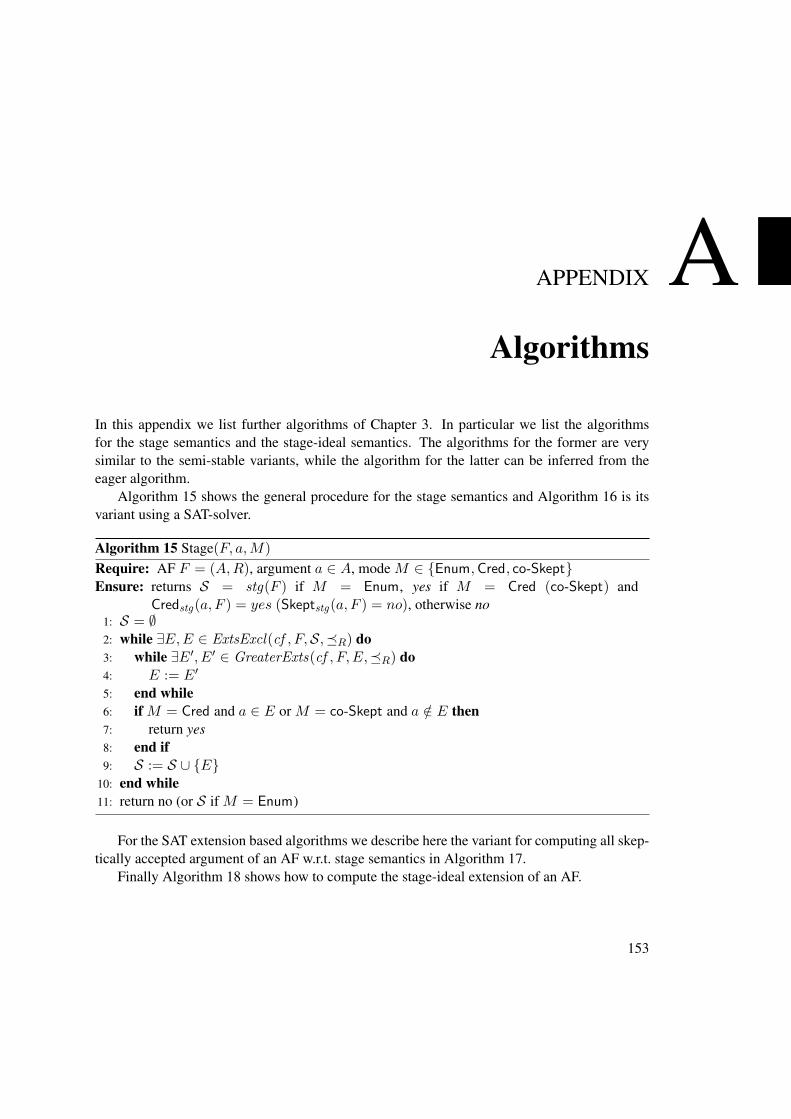
APPENDIX AAlgorithms

In this appendix we list further algorithms of Chapter 3. In particular we list the algorithmsfor the stage semantics and the stage-ideal semantics. The algorithms for the former are verysimilar to the semi-stable variants, while the algorithm for the latter can be inferred from theeager algorithm.

Algorithm 15 shows the general procedure for the stage semantics and Algorithm 16 is itsvariant using a SAT-solver.

Algorithm 15 Stage(F, a,M)

Require: AF F = (A,R), argument a ∈ A, mode M ∈ {Enum,Cred, co-Skept}Ensure: returns S = stg(F ) if M = Enum, yes if M = Cred (co-Skept) and

Credstg(a, F ) = yes (Skeptstg(a, F ) = no), otherwise no1: S = ∅2: while ∃E,E ∈ ExtsExcl(cf , F,S,�R) do3: while ∃E′, E′ ∈ GreaterExts(cf , F, E,�R) do4: E := E′



For the SAT extension based algorithms we describe here the variant for computing all skep-tically accepted argument of an AF w.r.t. stage semantics in Algorithm 17.

Finally Algorithm 18 shows how to compute the stage-ideal extension of an AF.

153

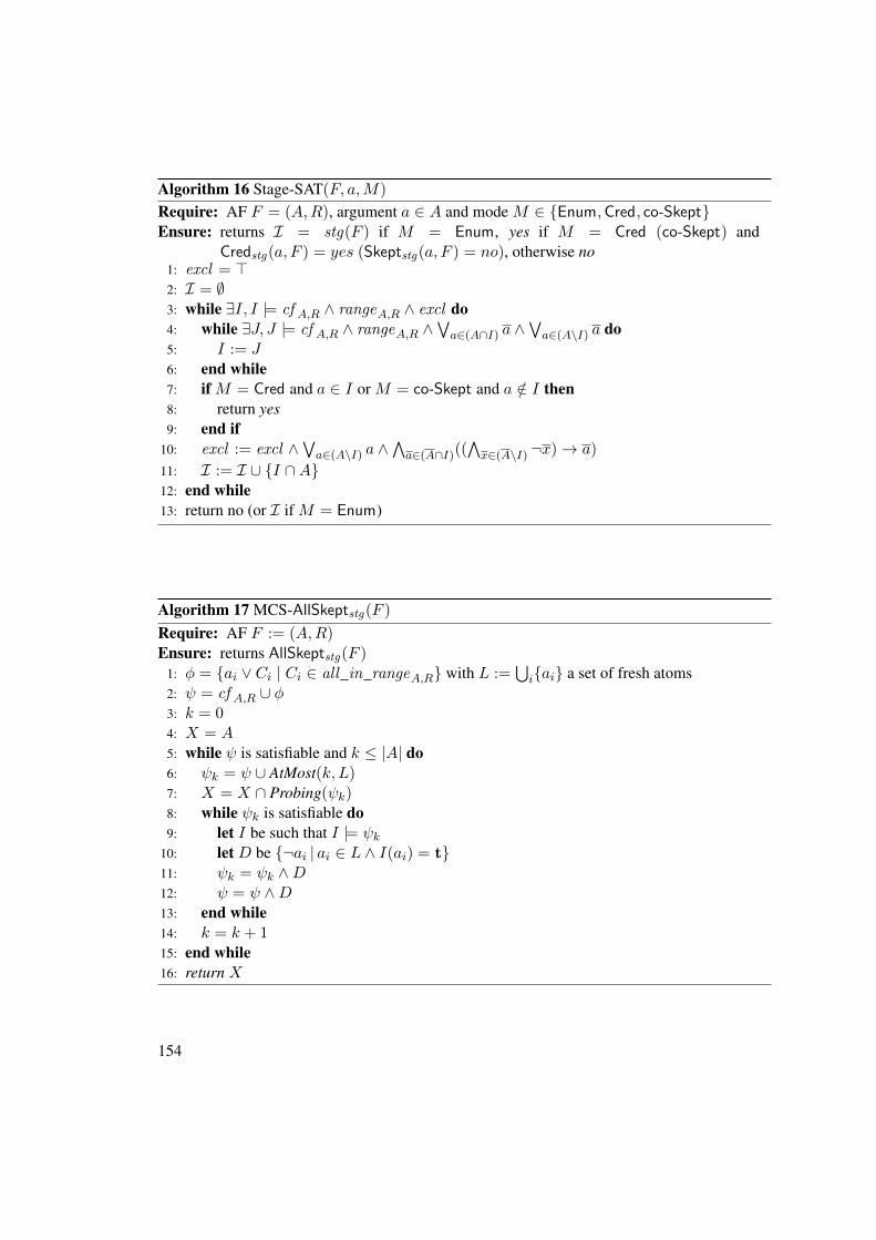
Algorithm 16 Stage-SAT(F, a,M)

Require: AF F = (A,R), argument a ∈ A and mode M ∈ {Enum,Cred, co-Skept}Ensure: returns I = stg(F ) if M = Enum, yes if M = Cred (co-Skept) and

Credstg(a, F ) = yes (Skeptstg(a, F ) = no), otherwise no1: excl = >2: I = ∅3: while ∃I, I |= cf A,R ∧ rangeA,R ∧ excl do4: while ∃J, J |= cf A,R ∧ rangeA,R ∧

∨a∈(A∩I) a ∧

∨a∈(A\I) a do


10: excl := excl ∧∨a∈(A\I) a ∧∧a∈(A∩I)((

∧x∈(A\I) ¬x)→ a)

11: I := I ∪ {I ∩A}12: end while13: return no (or I if M = Enum)

Algorithm 17 MCS-AllSkeptstg(F )

Require: AF F := (A,R)Ensure: returns AllSkeptstg(F )

1: φ = {ai ∨ Ci | Ci ∈ all_in_rangeA,R} with L :=⋃i{ai} a set of fresh atoms

2: ψ = cf A,R ∪ φ3: k = 04: X = A5: while ψ is satisfiable and k ≤ |A| do6: ψk = ψ ∪ AtMost(k, L)7: X = X ∩ Probing(ψk)8: while ψk is satisfiable do9: let I be such that I |= ψk

10: let D be {¬ai | ai ∈ L ∧ I(ai) = t}11: ψk = ψk ∧D12: ψ = ψ ∧D13: end while14: k = k + 115: end while16: return X

154

Algorithm 18 MCS-Stage-ideal(F )

Require: AF F = (A,R)Ensure: returns stg-idl(F )

1: X = MCS-AllSkeptstg(F )

2: return F |A|F (X)

155

APPENDIX BCurriculum Vitae

157

Johannes Peter WallnerCurriculum Vitae

Address: Vienna University of TechnologyInstitute of Information SystemsDatabase and Artificial Intelligence GroupFavoritenstrasse 9A-1040 Wien, Austria

Phone: +43-1-58801-18409Fax: +43-1-58801-9-18409E-Mail: [email protected]: http://www.dbai.tuwien.ac.at/user/wallner/Citizenship: AustriaBirthday: 13.5.1984

EducationUniversity

2011 - present • Ph.D. study, Vienna University of Technology.Supervisor: Stefan Woltran

2008 - 2010 •Master study, Vienna University of Technology:“Computational Intelligence”, passed with distinction.Thesis: A Hybrid Approach for Model-Based Random TestingSupervisor: Univ. Prof. Dr. Franz WotawaCo-supervisor: Univ. Ass. Dr. Bernhard Peischl

2003 - 2008 • Bachelor study, Vienna University of Technology: “Software& Information Engineering”

Participation in Doctoral Programme

2011 - present • Doctoral programme Mathematical Logic in Computer Science,Vienna University of Technology.

Participation in Doctoral Consortium/Summer School/Winter School

Feb. 2014 • Advanced Winter School on Reasoning Engines for RigorousSystem Engineering, ReRiSE 2014.

Jul. 2013 • Advanced Course on AI (ACAI) 2013 summer school; studentsession topic: Advanced Procedures for Hard Problems in Ab-stract Argumentation.

Jun. 2012 • Doctoral Consortium at the thirteenth conference on Prin-ciples of Knowledge Representation and Reasoning (KR)2012. Topic: Computational Properties of Abstract Dialecti-cal Frameworks.

Academic Working ExperienceProject Employment

Jun. 2013 - present • Project assistant in the Database and AI Group, Vienna Univer-sity of Technology.International project (Germany/Austria): Abstract DialecticalFrameworks: Advanced Tools for Formal Argumentation.Funded by Deutsche Forschungsgemeinschaft (DFG) and Aus-trian Science Fund (FWF) through project I1102Project leaders: Gerd Brewka and Stefan Woltran

Sept. 2012 - May 2013 • Project assistant in the Database and AI Group, Vienna Univer-sity of Technology.Project: SEE: SPARQL Evaluation and Extensions.Funded by WWTF – Wiener Wissenschafts-, Forschungs- undTechnologiefonds (ICT 12-015)Project leader: Reinhard Pichler

May 2011 - Aug. 2012 • Project assistant in the Database and AI Group, Vienna Univer-sity of Technology.Project: New Methods for Analyzing, Comparing, and SolvingArgumentation Problems.Funded by WWTF – Wiener Wissenschafts-, Forschungs- undTechnologiefonds (ICT 08-028)Project leader: Stefan Woltran

Other Project Activities

2012 - 2013 • Project member in bilateral project Austria/SlovakiaProject: New Directions in Abstract ArgumentationFunded by Slovenská akademická informaná agentúra (SAIA)and Österreichischer Austauschdienst (ÖAD); project number2012-03-15-0001Project coordinators: Jozef Siška, Comenius Univ. Bratislavaand Stefan Woltran

Reviewing

• ECAI 2012, ESSLLI 2013, CILC 2013 and LPNMR 2013

Professional Activities

• Fourth ASP Competition 2013, member of organizing commit-tee

• Assistance in writing project proposal (co-author): Abstract Di-alectical Frameworks: Advanced Tools for Formal Argumenta-tion, funded by DFG/FWF.

Research Visits

Apr. - Jun. 2012 • Gerhard Brewka, Leipzig University

Scientific Talks

16. Sep. 2013 • Advanced SAT Techniques for Abstract Argumentation.CLIMA’13

5. July. 2013 • SAT-based Argumentation Systems. Advanced Course on AI(ACAI) 2013, student session.

2. Apr. 2012 • Knowledge Base Change and Abstract Dialectical Frame-works. Dynamics of Argumentation, Rules and Conditionals(DARC) workshop.

28. Sept. 2011 • Making Use of Advances in Answer-Set Programming for Ab-stract Argumentation Systems. INAP’11

23. Aug. 2010 • A hybrid approach for model-based random testing. VALID’10

Awards and Grants

• ECCAI Travel Award for attending ACAI 2013

• Grant for attending doctoral consortium at KR 2012

• Distinguished Student Paper Prize for ”Complexity-SensitiveDecision Procedures for Abstract Argumentation“ at KR 2012

Teaching

• Course ”Abstract Argumentation“ at the Vienna University ofTechnology (winter 2012)

• Co-advisor for master thesis: Stefan Ellmauther, Abstract Di-alectical Frameworks: Properties, Complexity, and Implemen-tation, 2012

Language skills

• German (native)

• English (fluent)

Publications

Journals

[1] Wolfgang Dvorák, Matti Järvisalo, Johannes P. Wallner, and Stefan Woltran. Complexity-Sensitive Decision Procedures for Abstract Argumentation. Artificial Intelligence, 206:53–78, 2014.

[2] Axel Polleres and Johannes P. Wallner. On the relation between SPARQL1.1 and AnswerSet Programming. Journal of Applied Non-Classical Logics, 23(1–2):159–212, 2013.

Conferences and Workshops

[3] Hannes Strass and Johannes P. Wallner. Analyzing the Computational Complexity of Ab-stract Dialectical Frameworks via Approximation Fixpoint Theory. In Proceedings of the14th International Conference on Principles of Knowledge Representation and Reasoning,KR 2014, Vienna, Austria, July 2014. To appear.

[4] Mario Alviano, Francesco Calimeri, Günther Charwat, Minh Dao-Tran, Carmine Dodaro,Giovambattista Ianni, Thomas Krennwallner, Martin Kronegger, Johannes Oetsch, An-dreas Pfandler, Jörg Pührer, Christoph Redl, Francesco Ricca, Patrik Schneider, MartinSchwengerer, Lara K. Spendier, Johannes P. Wallner, and Guohui Xiao. The Fourth An-swer Set Programming Competition: Preliminary Report. In Pedro Cabalar and Tran CaoSon, editors, Proceedings of the Twelfth International Conference on Logic Programmingand Nonmonotonic Reasoning, LPNMR 2013, volume 8148 of Lecture Notes in ArtificialIntelligence, pages 42–53, Corunna, Spain, September 2013. Springer.

[5] Thomas Ambroz, Günther Charwat, Andreas Jusits, Johannes P. Wallner, and StefanWoltran. ARVis: Visualizing Relations between Answer Sets. In Pedro Cabalar andTran Cao Son, editors, Proceedings of the Twelfth International Conference on Logic Pro-gramming and Nonmonotonic Reasoning, LPNMR 2013, volume 8148 of Lecture Notes inArtificial Intelligence, pages 73–78, Corunna, Spain, September 2013. Springer.

[6] Günther Charwat, Giovambattista Ianni, Thomas Krennwallner, Martin Kronegger, An-dreas Pfandler, Christoph Redl, Martin Schwengerer, Lara K. Spendier, Johannes P. Wall-ner, and Guohui Xiao. VCWC: A Versioning Competition Workflow Compiler. In PedroCabalar and Tran Cao Son, editors, Proceedings of the Twelfth International Conferenceon Logic Programming and Nonmonotonic Reasoning, LPNMR 2013, volume 8148 ofLecture Notes in Artificial Intelligence, pages 233–238, Corunna, Spain, September 2013.Springer.

[7] Sylwia Polberg, Johannes P. Wallner, and Stefan Woltran. Admissibility in the AbstractDialectical Framework. In João Leite, Tran Cao Son, Paolo Torroni, Leon van der Torre,

and Stefan Woltran, editors, Proceedings of the 14th International Workshop on Compu-tational Logic in Multi-Agent Systems, CLIMA 2013, volume 8143 of Lecture Notes inArtificial Intelligence, pages 102–118, Corunna, Spain, September 2013. Springer.

[8] Johannes P. Wallner, Georg Weissenbacher, and Stefan Woltran. Advanced SAT Tech-niques for Abstract Argumentation. In João Leite, Tran Cao Son, Paolo Torroni, Leonvan der Torre, and Stefan Woltran, editors, Proceedings of the 14th International Work-shop on Computational Logic in Multi-Agent Systems, CLIMA 2013, volume 8143 of Lec-ture Notes in Artificial Intelligence, pages 138–154, Corunna, Spain, September 2013.Springer.

[9] Gerhard Brewka, Stefan Ellmauthaler, Hannes Strass, Johannes P. Wallner, and StefanWoltran. Abstract Dialectical Frameworks Revisited. In Francesca Rossi, editor, Pro-ceedings of the 23rd International Joint Conference on Artificial Intelligence, IJCAI 2013,pages 803–809, Beijing, China, August 2013. AAAI Press / IJCAI.

[10] Wolfgang Dvorák, Sarah A. Gaggl, Johannes P. Wallner, and Stefan Woltran. MakingUse of Advances in Answer-Set Programming for Abstract Argumentation Systems. InHans Tompits, Salvador Abreu, Johannes Oetsch, Jörg Pührer, Dietmar Seipel, MasanobuUmeda, and Armin Wolf, editors, Proceedings of the 19th International Conference on Ap-plications of Declarative Programming and Knowledge Management, INAP 2011, RevisedSelected Papers, volume 7773 of Lecture Notes in Artificial Intelligence, pages 114–133.Springer, 2013.

[11] Günther Charwat, Johannes P. Wallner, and Stefan Woltran. Utilizing ASP for Generatingand Visualizing Argumentation Frameworks. In Michael Fink and Yuliya Lierler, editors,Proceedings of the Fifth Workshop on Answer Set Programming and Other ComputingParadigms, ASPOCP 2012, pages 51–65, Budapest, Hungary, September 2012.

[12] Stefan Ellmauthaler and Johannes P. Wallner. Evaluating Abstract Dialectical Frameworkswith ASP. In Bart Verheij, Stefan Szeider, and Stefan Woltran, editors, Proceedings of theFourth International Conference on Computational Models of Argument, COMMA 2012,volume 245 of Frontiers in Artificial Intelligence and Applications, pages 505–506, Vi-enna, Austria, September 2012. IOS Press.

[13] Wolfgang Dvorák, Matti Järvisalo, Johannes P. Wallner, and Stefan Woltran. Complexity-Sensitive Decision Procedures for Abstract Argumentation. In Gerhard Brewka, ThomasEiter, and Sheila A. McIlraith, editors, Proceedings of the 13th International Conferenceon Principles of Knowledge Representation and Reasoning, KR 2012, pages 54–64, Rome,Italy, June 2012. AAAI Press.

[14] Wolfgang Dvorák, Sarah A. Gaggl, Johannes P. Wallner, and Stefan Woltran. MakingUse of Advances in Answer-Set Programming for Abstract Argumentation Systems. InSalvador Abreu, Johannes Oetsch, Jörg Pührer, Dietmar Seipel, Hans Tompits, MasanobuUmeda, and Armin Wolf, editors, Proceedings of the 19th International Conference on

Applications of Declarative Programming and Knowledge Management, INAP 2011, pages117–130, Vienna, Austria, September 2011.

[15] Stefan Mohacsi and Johannes P. Wallner. A hybrid approach for model-based randomtesting. In Lydie du Bousquet, Juho Perälä, and Pascal Lorenz, editors, Proceedings of theSecond International Conference on Advances in System Testing and Validation Lifecycle,VALID 2010, pages 10–15, Nice, France, August 2010. IEEE.

Miscellaneous

[16] Günther Charwat, Wolfgang Dvorák, Sarah A. Gaggl, Johannes P. Wallner, and StefanWoltran. Implementing Abstract Argumentation - A Survey. Technical Report DBAI-TR-2013-82, Technische Universität Wien, 2013.

[17] Hannes Strass and Johannes P. Wallner. Analyzing the Computational Complexity of Ab-stract Dialectical Frameworks via Approximation Fixpoint Theory. Technical Report 2,Computer Science Institute, Leipzig University, 2013.

[18] Wolfgang Dvorák, Matti Järvisalo, Johannes P. Wallner, and Stefan Woltran. CEGARTIX:A SAT-Based Argumentation System. Presented at the Pragmatics of SAT Workshop (PoS2012), 2012.

[19] Wolfgang Dvorák, Sarah A. Gaggl, Johannes P. Wallner, and Stefan Woltran. Making Useof Advances in Answer-Set Programming for Abstract Argumentation Systems. TechnicalReport DBAI-TR-2011-70, Technische Universität Wien, 2011.

[20] Johannes P. Wallner. Hybrid approach for model-based random testing. Master’s thesis,Technische Universität Wien, Institut für Informationssysteme, 2010.

Last updated: April 2, 2014

References

Associate Prof. Dr. Stefan WoltranVienna University of TechnologyInstitute of Information SystemsDatabase and Artificial Intelligence GroupFavoritenstraße 9-11A-1040 Vienna, Austria

Prof. Dr. Reinhard PichlerVienna University of TechnologyInstitute of Information SystemsDatabase and Artificial Intelligence GroupFavoritenstraße 9-11A-1040 Vienna, Austria

Prof. Dr. Gerhard BrewkaLeipzig UniversityComputer Science InstituteIntelligent Systems DepartmentAugustusplatz 1004109 Leipzig, Germany

Documents

Complexity Results and Algorithms for Argumentation · in diverse applications including legal reasoning, E-Democracy tools, medical applications and many more. An integral part of