Complexity, Language, and Life:Mathematical Approaches

Edited byJohn L. Casti and Anders Karlqvist

Springer-VerlagBerlin Heidelberg New York Tokyo

John L. Casti

International Institute for Applied Systems Analysis2361 Laxenburg, Austria

Anders Karlqvist

Swedish Academy of Sciences10110 Stockholm, Sweden

Mathematics Subject Classification (1980): 9202,9302

ISBN 3-540-16180-5 Springer-Verlag Berlin Heidelberg New York TokyoISBN 0-387-16180-5 Springer-Verlag New York Heidelberg Berlin Tokyo

© International Institute for Applied Systems Analysis, 1986AU rights reserved. No part of this publication may be reproduced, stored in a retrievalsystem, or transmitted, in any form or by any means, electronic, mechanical, photocopying,recording or otherwise, without the prior permission of the copyright owner.

Printed in Germany

Printing: Beltz, Hemsbach/BergstralleBinding: Schaffer, Griinstadt

2141/3145-543210

Preface

In May 1984 the Swedish Council for Scientific Research conveneda small group of investigators at the scientific research station atAbisko, Sweden, for the purpose of examining various conceptualand mathematical views of the evolution of complex systems. Thestated theme of the meeting was deliberately kept vague, with onlythe purpose of discussing alternative mathematically basedapproaches to the modeling of evolving processes being given as aguideline to the participants. In order to limit the scope to somedegree, it was decided to emphasize living rather than nonlivingprocesses and to invite participants from a range of disciplinaryspecialities spanning the spectrum from pure and appliedmathematics to geography and analytic philosophy.

The results of the meeting were quite extraordinary; while therewas no intent to focus the papers and discussion into predefinedchannels, an immediate self-organizing effect took place and thedeliberations quickly oriented themselves into three mainstreams: conceptual and formal structures for characterizing sys­tem complexity; evolutionary processes in biology and ecology;the emergence of complexity through evolution in natural lan­guages. The chapters presented in this volume are not the proceed­ings of the meeting. Following the meeting, the organizers felt thatthe ideas and spirit of the gathering should be preserved in somewritten form, so the participants were each requested to produce achapter, explicating the views they presented at Abisko, writtenspecifically for this volume. The results of this exercise form thevolume you hold in your hand.

Special thanks for their help in various phases of organizationsof the meeting and arrangement of the publication of this volumeare due to M. Olson, P. Sahlstrom, and R. Ouis.

December 1985 John Casti, ViennaAnders Karlqvist, Stockholm

The International Institute for Applied Analysisis a nongovernmental research institution, bringing together scien­tists from around the world to work on problems of commonconcern. Situated in Laxenburg, Austria, IIASA was founded inOctober 1972 by the academies of science and equivalent organi­zations of twelve countries. Its founders gave IIASA a uniqueposition outside national, disciplinary, and institutional bound­aries so that it might take the broadest possible view in pursuing itsobjectives:

To promote international cooperation in solving problems arisingfrom social, economic, technological, and environmentalchange

To create a network of institutions in the national member organi­zation countries and elsewhere for joint scientific research

To develop and formalize systems analysis and the sciences con­tributing to it, and promote the use of analytical techniquesneeded to evaluate and address complex problems

To inform policy advisors and decision makers about the potentialapplication of the Institute's work to such problems

The Institute now has national member organizations in thefollowing countries:

Austria - The Austrian Academy of Sciences; Bulgaria - TheNational Committee for Applied Systems Analysis and Manage­ment; Canada - The Canadian Committee for IIASA; Czecho­slovakia - The Committee for IIASA of the Czechoslovak SocialistRepublic; Finland - The Finnish Committee for IIASA; France ­The French Association for the Development ofSystems Analysis;German Democratic Republic - The Academy of Sciences of theGerman Democratic Republic; Federal Republic of Germany ­Association for the Advancement of IIASA; Hungary - TheHungarian Committee for Applied Systems Analysis; Italy - TheNational Research Council; Japan - The Japan Committee forIIASA; Netherlands - The Foundation IIASA - Netherlands;Poland - The Polish Academy of Sciences; Sweden - The SwedishCouncil for Planning and Coordination of Research; Union ofSoviet Socialist Republics - The Academy ofSciences ofthe Unionof Soviet Socialist Republics; United States of America - TheAmerican Academy ofArts and Sciences;

I:

List of Contributors

David Berlinski, Institut des Hautes Etudes Scientifiques,35 Route de Chartres, 91440 Bures-sur-Yvette, France

John L. Casti, International Institute for Applied SystemsAnalysis, A-2361 Laxenburg, Austria

Peter Gould, Department of Geography, College of Earth andMineral Sciences, The Pennsylvania State University,302 Walker Building, University Park, Pennsylvania 16802,USA

Vlf Grenander, Mittag-Leffler Institute, Auravagen 17, S-10262Djursholm, Sweden

Jeffrey Johnson, Centre for Configurational Studies, DesignDiscipline, Faculty of Technology, The Open University,Walton Hall, Milton Keynes MK7 6AA, England

Howard H. Pattee, Department of Systems Science, T. J. Wat­son School of Engineering, State University of New Yark atBinghampton, Binghampton NY 13901, USA

Robert Rosen, Department of Physiology and Biophysics,Dalhousie University, Nova Scotia, Canada, B3H 4H7

Karl Sigmund, Institute of Mathematics, University of Vienna,Strudelhofgasse 4, A-1090 Wien, Austria

Nils Chr. Stenseth, Zoological Institute, University of Oslo, POBox 1050, B1indern, Oslo 3, Norway

Rene Thorn, Institut des Hautes Etudes Scientifiques, 35 Routede Chartres. 91440 Bures-sur-Yvette, France

Table of Contents

1. Allowing, forbidding, but not requiring:a matnematic for a human world . . . . .Peter Gould

2. A theory ofstars in complex systemsJeffrey Johnson

3. Pictures as complex systemsUlf Grenander

4. A survey ofreplicator equationsKarl Sigmund

1

21

62

88

5. Darwinian evolution in ecosystems: a survey of someideas and difficulties together with some possible solu-tions . . . . . . . . . . . . . . . . . . . . . . . . .. 105Nils Chr. Stenseth

6. On system complexity: identification, measurement,and management . . . . . . . . . . . . . . .. 146John L. Casti

7. On information and complexityRobert Rosen

174

8. Organs and tools: a common theory ofmorphogenesis 197Rene Thorn

9. The language of lifeDavid Berlinski

231

10. Universal principles of measurement and languagefunctions in evolving systems 268Howard H. Pattee

Introduction

John L. Casti and Anders Karlqvist

Complexity and the Evolution of Living Systems

One of the most evident features distinguishing living from nonliving systemsis the tendency for living processes to evolve ever more complex structural andbehavioral modes during the course of time. This characteristic has been observedin lowly protozoa and in highly evolved linguistic and social communities, and hasbeen variously labeled "negentropy", "variety". "information". or just plain com­plexity. The understanding and explanation of the trend toward the complexifica­tion of living things forms the heart of any research program in the biological,social, or behavioral sciences.

How does complexity emerge and what do we even mean when we speak of asystem as being complex? In everyday language, complexity is associated withstructural features such as large numbers of system components, high levels ofconnectivity between subsystems, feedback and feedforward data paths that aredifficult to trace. and so on. Complexity is also associated with behavioral charac­teristics such as counterintuitive reactions, surprises, multiple modes of opera­tion, fast and slow system time scales, and irreproducible surprises. While thestructural features are, by and large, objective properties of the system per se,the behavioral components of complexity are decidedly subjective: what is coun­terintuitive, surprising, and so on is as much a property of the system doing theobserving as it is a feature of the process under study. Thus, any mathematicalformulations of the notion of complexity must respect the subjective, as well asthe objective, aspects of the concept. In this volume, the chapters by Rosen andCasti address both aspects of the complexity question. Casti argues that complex­ity emerges from the interaction between the system and its observer, whileRosen introduces the idea of an activation-inhibition pattern to characterize theinformational interaction, and then uses this concept to speak of complexity.Both of these chapters put forth strong arguments for the case that complexity ofliving systems is a contingent, rather than intrinsic, property of the system. andany theory of complexity management and control must start from this basis.

The explicit consideration of evolutionary processes in biology is taken up inthe chapters by Sigmund and Stenseth. Stenseth reviews the essential com­ponents of the Darwinian theory: reproduction, variation, inheritance. and selec­tion, and considers the issue of what kinds of mathematical models we need inorder to capture the Darwinian view in operational form. His conclusion is that thenumerous controversies surrounding the Darwinian paradigm in no way provide evi­dence for rejecting it, but rather point to the need to extend and improve our

XII

models in various directions. The chapter by Sigmund offers an intriguingmathematical structure suitable for capturing many of the most important featuresof evolving systems, the so-called "replicator" dynamics. The term is taken fromDawkins' work on general phenotypic evolution and here Sigmund shows how thegeneral structure of the replicator equations covers a range of evolutionaryphenomena stretching from population genetics and prebiotic evolution to popula­tion ecology and animal behavior. As a counterpoint to Darwinism, the chapter byThom presents some speculative views on the way in which energetic constraints,together with a few genericity arguments, provide a key for understanding therelations of tools and organs within the context of embryology. Thom's argument isthat constraints plus genericity force the embryo to develop along one of a verysmall number of paths characterized by archetypical geometric forms. As Thomemphasizes, such forms are imaginary entities offering no possibility for experi­mental prediction or verification; nonetheless, his claim is that they provide thebasis for major theoretical advances bypassing the traditional Darwinian view.

The degree to which the evolutionary paradigm of biology mirrors the struc­ture of a natural language is considered in the chapter by Berlinski. His point ofview is to examine the claim that life, on some level, is a language-like system. Heconcludes that if life is a language-like system, then the neo-Darwinian theory isdeficient in its repertoire of theoretical ideas. On the other hand, if life is not alanguage-like system, then the neo-Darwinian theory is singular in that it fails toexpiain or predict the properties of systems that are in some measure close tolife. During the course of making these arguments, Berlinski touches on a numberof ideas treated in the other chapters, such as complexity, randomness, informa­tion, pattern, and form.

The connection between the concept of measurement and the development ofhuman language is explored in the chapter by Pattee. He argues that it is only byviewing measurement and language in an evolutionary context that we can appreci­ate how primitive and universal are the functional principles from which ourhighly specialized forms of measurement and language arose. Pattee's position isthat the generalized functions of language and measurement form a semanticallyclosed loop, which is a necessary condition for evolution. The chapter closes withsome provocative arguments for why current theories of measurement andlanguage do not satisfy the semantic closure requirement for evolution, and asuggestion is offered for a new approach to designing adaptive systems that havethe possibility for greater evolutionary and learning potential than existing artifi­cial intelligence models.

Mathematical and Human Mairs

The role of mathematics outside of mathematics itself has always been some­what unclear and ill-defined. What has been clear is that every generation's prob­lems, especially in the social and behavioral sciences, seem to far exceed themathematical tools available, resulting in a continuing need to both develop newmathematical concepts and to examine ways in which the existing "abstract non­sense" of the pure mathematician can be recast in a form usable to the practi­tioner.

XIII

In the opening chapter of this volume. Peter Gould examines some of theproblems of mathematicizing the physical, biological, and human worlds. He pointsout that over most of history, mathematics has been driven by the problems posedby practical, everyday living, ultimately addressing the question of whethermathematics is reducible to mechanical operations on sets of objects. He concludesthat if this is so, then there is no possibility for a complete mathematicization ofthe human world.

An illustration of the way in which ideas from pure mathematics can be usedto develop a language for speaking about human processes is provided in thechapter by Johnson. In his report, classical ideas from algebraic topology areused to associate a simplicial complex with a given human situation. The connectivestructure of the complex is then employed to infer various "deep structures"associated with the social situation. During the course of developing this struc­ture, Johnson shows how the introduction of numerous concepts not entering intoclassical algebraic topology can playa significant role in teasing out the structureof the human situation.

The chapter by Grenander approaches the role of mathematics in humanaffairs from a different angle. Grenander's idea is that in order to speak aboutpictures and patterns, it is first necessary to develop an entire a.lgebra. of pat­terns. This algebra is then employed to mathematically characterize complexvisual phenomena, and forms the basis of numerous pattern formation and recogni­tion procedures. As Grenander points out, such an approach is really "mathemati­cal engineering"; we build logical structures using the algebra of patterns. just asengineers build mechanical, electrical, or other physical structures.

CHAPTER 1

Allowing, Forbidding, but not Requiring:A Mathematic for a Human World

Peter Gould

In Morris Kline's extraordinarily thoughtful Mathematics: The Loss of Cer­tainty (Kline, 1980), one aspect emerges clearly: over by far the greatest part ofits history, mathematics has been driven by the need to describe the physicalworld of things. The distinction between pure and applied mathematics did notemerge until comparatively recently; no sharp distinction was made betweenmathematics and science in the seventeenth and eighteenth centuries. and all thegreat names contributed to the vast overlapping area between the two. In brief"there was some pure mathematics but no pure mathematicians" (Kline. 1980, p281). It is unfortunate that. just as the biological and human sciences started tohive off from philosophy as separate fields of inquiry, so mathematics began todetach itself from the physical sciences. First, this means that few mathemati­cians today have ever been truly challenged by the biological and human sciences.with the result that old and inappropriate forms of mathemetics have been bor­rowed from the realm of the physical world to distort descriptions of the biologi­cal and human worlds. Second, the possibilities for creating new and appropriatequalitative mathematics have been diminished as mathematicians look increasinglyto mathematics itself, rather than to the challenges beyond their distressinglyprivate realm of discourse.

But like war and generals. mathematics is too important to leave to themathematicians. Such a statement. unless it is read correctly, will not please manymathematicians (nor did it please the generals). but it may still be consideredseriously by the few who have acquired a deep and intimate knowledge of the his­tory of their own field. Like anyone of many human endeavors. mathematics can­not reflect upon itself from the inside, but requires that creative sense of tensionthat the philosophical stance has always provided at its best. The human meaningof mathematics does not reside in mathematics, but in the larger arena of humandiscourse that places this particular, and quite peculiar, form of inquiry in rela­tion to other aspects of our intention to know.

2

A Backcloth for Thinking

P. Gould

I would like to consider some of the problems of mathematization in the phy­sical, biological, and human worlds, and I hope it will be considered appropriatethat we start with the human - the world of ourselves. This is a curious, self­reflective world, and its capacity for self-reflection, for thinking about itself, issurely its most outstanding characteristic. Atoms and animals do not conceive oflaws, nor do they generate the functional equations commonly used to describethem. In contrast, we are distinguished by that very ability. For this reason, it isperhaps appropriate to sketch a broad framework of concern within which we candiscuss mathematically more specific questions and requirements. With theresponsibility to represent the human sciences in this book, I hope you agree thatit is entirely appropriate that we first take a step backwards - a sort of intellec­tual deep breath - and think about this world that is us; think about the cre­ation of mathematics within and from out of this world; and then think about thatsudden backward twist when mathematics is used to describe the world from whichit originally arose. In doing so, it may seem that we are in a rather different realmof inquiry than some of the other contributions in this book, and yet per:haps weare always in this larger realm of thinking - even if we may not always realize it.

The mundane roots or mathematics

Not long ago, I read in L'Ezpress (17-23 fevrier, 1984) a review of Giorelloand Morini's .Fb.raboles et catastrophes: Entretiens avec Rene Thorn (1983), inwhich the reviewer wrote with great aplomb "Thus, mathematical structures havecome before their use in physics, and not the reverse". Nowhere, perhaps, is thestriking contrast between the French Cartesian approach to science, and theAnglo-Saxon empirical approach highlighted more vividly. It is the contrastbetween the creation of a priori structures into which the world is forced, andthe creation of careful descriptions of the world which later suggest appropriatemathematical structures. The reviewer's mistake is a common one, although quitenatural if the history of mathematics is not there to inform us about the facts. Asan Anglo-Saxon, and one concerned with historical veracity, let me suggest, verygenerally and up to about one hundred years ago, that far from mathematicalstructures being created for their own sake, and then being applied to areas of'scientific inquiry, the weight of evidence is for exactly the reverse. That is tosay, over most of its history mathematics has been positively driven by therequirements and difficulties posed by the problems of practical, everyday living,as well as by those appearing in the world of physical science as we know it today.Such problems range from tallying sheep, building temples and pyramids withsquare corners, surveying field boundaries after floods, and other, literally mun­dane, tasks, to creating new algebras and topological structures in order todescribe events on the quantum and cosmological scales.

Some mathematicians still know the story, but let me remind others of theinfinitesimals of Isaac Newton, the extensions to the calculus by James Maxwell,the algebras and numbers of William Hamilton that were so outrageous in theirtime, and then point to the driving force behind Lagrange, Leverrier,

11

ALLowing. Forbidding, But Not Requiring 3

Legendre ... and the literally scores of other distinguished mathematicians of theseventeenth to nineteenth centuries, who sought to describe faithfully the physi­cal world. It is the intentional, and perhaps insatiable, curiosity to describe theworld, that Greek legacy that pushes the questions to the limits (and may yet des­troy us), that invariably comes before the mathematics, that often informsmathematicians where the deep problems lie, and that nourishes those who searchfor the mathematical solutions. John von Neumann knew this well, and stated soexplicitly. And to accept this is not to deny in the least the desire of those whoseek to develop mathematics for its own sake, and in giants like Friedrich Gaussand Henri Poincare we see how both mathematics and science are illuminated by.such penetrating thinking. Yet as a geographer, I cannot help noting, in a some­what mischevious mood, that even the distribution that bears Gauss's name wasdevised to minimize the error in his instruments when he was making maps for theDuke of Hannover - a sound, descriptive enterprise going back to Babylon.

Now it is equally true that we can also point, in more recent times - the lasteighty years? - to the reverse; namely, to the prior existence of mathematicalstructures which later became not just useful, but essential for the developmentof science. For example, Albert Einstein reaches for the tensor calculus of Ricciand Levi-Givita (created only a few years before), and Walter Heisenberg strugglesto devise algebraic operations for rectangular tables of values, until Max Borntells him to go and study matrix algebra - already well-developed. In these partic­ular cases, the appropriate mathematical structures were already in place, buteven here the thinking about the physical world. from the cosmological to thequantum level, preceded the applications.

Why am I trying to direct thinking towards this brief, and necessarily super­ficial, historical review of mathematics? Because I want to point to the fact thathistorically, and even today, the physical sciences have, in general, set an impec­cable example of thinking about the phenomena of interest, and only then devis­ing and creating the mathematics that seems to be called forth by the descriptiverequirements. The things themselves suggest the mathematical structures thatmust come into being to describe the physical phenomena that falls under thescrutiny of our curious gaze. What are the only other possibilities? First, tochoose an already existing mathematical structure, and then run around the worlddesperately seeking something that will fit it. Rather like Diogenes searching foran honest man, our journals are full of reports of methodologists searching for anhonest appUcation. However, I think it is necessary to reflect whether most of thereports constitute science, in the sense that they genuinely illuminate a part ofour world.

Second, we can borrow unthinkingly the mathematical structures devised todescribe one aspect of our world, and use them, equally unthinkingly, to describeanother aspect. If we take the mathematical structures devised to describe theworlds of celestial mechanics, statistical mechanics, quantum mechanics, contin­uum mechanics ... and just plain mechanics, and then map the human worldunthinkingly onto such structures, is it possible that the human world sodescribed can look anything but mechanical? In brief, does the mathematical"language" chosen allow the description, and allow our thinking, to appear as any­thing but mechanistic?

4

The meaning or mathematics

P. GouLd

Now mechanism is a world of lawful statements, statements we make aboutthings in essentially their deterministic relations. And, simply as a stage aside, Ido not want to argue the deterministic versus the probabilistic here. Throwingsome probability distributions into the arena of methodological discourse does not,for me, solve the fundamental problems in the human sciences. It merely sweepsthem under the rug, so that the real questions of transcending both approachesrecede into concealment from our thinking. As for the purely statistical approach,which was so popular in the human sciences until a few years ago, it condemns ahuman scientist to be a calculator of moments of distributions. Quite apart fromthe shallowness of such descriptions, and the shallowness of the questions theypurport to address, I cannot think of anything more boring as a lifetime's work.

Whether we consider deterministic or probabilistic descriptions, as theyhave been traditionally expressed, both are essentially functional in form. Thismeans that the cog-wheel variables on the right-hand side of the equation turn andgrind out, mechanically, on the left-hand side either a single value, or a mean valuesmeared with a bit of variance. The mechanical coupling of the conventional binaryoperations used on the set of real numbers is essentially the same, whether themodel is deterministic or probabilistic. In the human world, we need to movebeyond this simplistic dichotomy that arises from the descriptive requirements ofthe physical and biological worlds (where they may be perfectly adequate), to thefundamental facts of consciousness, reflection, and informed choice - not simplyconditioned behavior - in the human world. The mathematics must enable non­mechanical interpretation in allowing, forbidding, but not requ1.T1.nggeometries. This, as we shall see, may be a contradiction if claims are valid thatall mathematics is ultimately mechanical by its reduction to logically consistentoperations. This, for me, is a frontier question for which I seek your mostpenetrating thought and insight. It may be, in a very deep sense, that the humanworld is not mathematizable. Which is not to say that we do not take certainaspects of the human world, and map them with enormously severe many-to-onemappings onto mechanistic structures devised in the physical world. For example,entropy maximization models (Wilson, 1970), straight out of Boltzmann, take countsof people, and counts of costs between residences and workplaces, and after someheroic assumptions, and a series of computer iterations, find a most-likely distri­bution that best fits the numbers of the journey-to-work census for a particularcity. The result is a piece of social physics whose Langrangians tell us that aresidential area far from the work places is less accessible than those close to thework places. Not terribly illuminating, and not terribly helpful when it comes toplanning changes in the structure of the city to create a more humane and equi­table world. We have crushed away so much in the mapping that constitutes ourmechanical analogy that we cannot do very much with a solution that representsthe most general case of numbers distributed in a constrained box.

This frontier question - whether the tyranny of the conventional binaryoperation forces mathematics and, therefore, the parts of our world described bymathematics, to be mechanical - this question leads us to reflect upon the meaningof mathematics itself. And here, as elsewhere in this chapter, I rely heavily upon

AUowt71.g, Forbtd,cH71.g, But Not Requtrt71.g 5

the thinking of Martin Heidegger, who has reflected so deeply upon the originalUr-meaning of so many words we use daily. Unfortunately, the words used now havemade a long journey through time from the Greek world where they were firstcoined, used, and reflected their original human meaning. To recapture one par­ticular meaning, let us read Heidegger carefully for a moment (1977, p 116):

Modern physics is called mathematical because, in a remarkable way, it makesuse of a quite specific mathematics. But it can proceed mathematically in thisway only because, in a deeper sense, it is already itself mathematical. Ta.ma.thema.ta. means for the Greeks that which man knows in advance in hisobservation of whatever is and in his intercourse with things ...

He then goes on to elaborate on the characteristic of exactitude in physics,through the use of measurement, number, and calculation, where physics is "theself-contained system of motion of units of mass related spatiotemporally". It isobvious that we are extraordinarily close to Arthur Eddington (1935) here, withphysics as a closed, self-contained system - in a sense, Heidegger's "objectsphere". But then Heidegger continues (1977, p 120):

The humanistic sciences, in contrast, indeed all the sciences concerned withlife, must necessarily be inexact Just in order to remain rigorous... Theinexactitude of the historical sciences is not a deficiency, but is only the ful­fillment of a demand essential to this type of research.

Now if the fundamental meaning of exactitude is grounded upon number and binaryoperation, and inexactitude is a necessary condition for the historical or reconsti­tutive sciences to be rigorous, we cannot approach and illuminate the humansphere through the mathematics (the ta mathemata) of the physical sciences.And let us recall that this has traditionally been a mathematics of binary opera­tions on sets of numbers - usually the reals - for which the continuum is requiredas a mathematical definition. In this classical analytical world, inexactitude maysuggest the probabilistic smearings of the statistician, but these only represent aloosening up, a fuzzying operation after the creation of deterministic operationsdevised during the classical phase of the physical sciences. Instead of trying totidy things up by the contradictory use of probabilistic smears, perhaps weshould go back to the beginning and see what the human world, with real humanbeings center stage, is trying to say to us. This return to the clearing in theforest would be in the best traditions of classical science, even though the pathdimly seen through the trees may not lead in the same direction as the one we arefollowing now. Even to think of a mathematics that transcends the conventionaldeterministic-probabilistic dichotomy may constitute a challenge to modernmathematicians who are willing to leave classical analysis behind them.

In brief, we cannot employ conventional, physically inspired forms ofmathematics in the human sciences, not if we wish to pay reverent heed to thatworld of conscious, sentient beings with the capacity to reflect upon any state­ment or description we make of them. And I use the rather poetic phrase "to payreverent heed" with Heidegger, because it is here that our word theory isgrounded in the Greek theoria (Heidegger, 1977, p 163). Its two parts are thea,meaning outward appearance, the outward appearance we hear in our own wordtheatre; and horao, which means to look attentively, to view closely. Theoria -

6 P. GouLd

theory - is to look attentively at outward appearance. But there are perhaps evendeeper roots, because with a slightly different stress the Greeks could also hearin theoria both thea. and efra. Thea is goddess, and for Parmenides atetheiaappeared as a goddess. And a-letheia is liitheia. or concealment. negated in theGreek by the a, to create unconcealment that for the Greeks was the truth. Orais reverence, respect, and honor. so theoria now becomes the "reverent payingheed to the unconcealment of what presences" (Heidegger. 1977. p 164).

And now the long journey from the Greek world to us begins. a journey of suc­cessive translations, each of which constitutes a many-to-one mapping in whichthe original meaning is crushed out and lost. The Romans translate theoria ascontemplatio. and the templum of contemplatio has in it "to cut". so that now wehear our own word. template. For what is a template but something createdbeforehand into which something later must fit - and if it does not, we cut itdown. and chop it up, and force it until it does fit - usually with inappropriateapplications of least-squares, or a myriad of other forcing acts that we euphemisti­cally call "estimation procedures".

So what do we regard as our fundamental task as biological and human scien­tists? To pay reverent heed with the Greeks to allow that which is to come out ofconcealment? Or shall we cut up and shape and force into our preexisting templatethat which is in order that it shall become that which we want it to be? And I can­not help commenting here on the contrast between the scientific approaches ofRosalind Franklin (Sayre. 1975). Barbara McClintock (Keller, 1983), and Janet Row­ley (Vines. 1984), and those a priori Roman templaters we call the model builders.The first. Rosalind Franklin, spent seven years paying reverent heed to hundredsof X-ray crystallography photographs, and the double-helix diagram was found inher notes after her early death. The second, Barbara McClintock. was ridiculedfor years because she paid reverent heed to transposable genetic fragments, untilshe was awarded the Nobel prize much later (she actually used the phrase "youhave to listen to the material"). The third. Janet Rowley. spent 25 years lookingat the translocations of chromosomes, and so opened. almost single-handedly, animportant and growing area of contemporary medical and cancer research. Is itpossible that some women in our Western culture have a gentler Greek mode ofquestioning than many of the arrogant Roman templaters?

Let me suggest that after years of Roman arrogance. we try once more thegentler Greek mode, particularly as we approach the difficult task of thinkingabout the requirements for a mathematics that will describe. and allow that whichis to come forth. without too much of the severe. a priori templating. Without,that is. so much forcing by severe many-to-one mappings of the human materialsonto constrained structures that we know in advance (ta mathemata) the socialphysics that must be the conclusion. Let us also see the process of mathematicaldescription in the larger context that constitutes human interest and inquiry. Asscientists, we must always see mathematics as part of, as a contributor to, a muchlarger endeavor. For this task, I want to use the three perspectives of JurgenHabermas (1971) as temporary pegs on which to hang our thinking. rather than asexclusive categories with which to fragment our thinking still further. As we shallsee, his perspectives are actually intertwined and connected viewpoints thatinform and shape each other.

Ii

AUOW~fl.I1. ForlJ~dd~fl.g. But Not Requ~r~fl.g

Technical. hermeneutic. and elDancipatory perspectives

7

At the start of any inquiry, we have to choose to observe some things and notothers, and so we face the severe responsibility of thinking about what consti­tutes useful and fruitful definitions. We can never, of course, be sure about theseuntil they have been tried, either to succeed or to fail in illuminating an aspect ofour world. In their own sphere, mathematicians know all about these, often facingthe same problems of trial and error, and therefore take such initial responsibili­ties seriously. Many in the human sciences do not, or they appear to think thatthe matter of definitions - of sets and operations and relations - is so obvious,even banal, that it is trivial and naive even to mention this first, but always cru­cial, step. Always crucial. in the literal sense of a crossing point, because it ishere that we take our first step along one of a number of possible paths, so thatvirtually everything we can say thereafter is founded upon the choices we makehere. We then have the further obligation of thinking about how we shall observeand record the relations between the sets, what operations we shall allow. how weshall notate the elements and operations, and even how we might express ourthoughts symbolically or graphically. All these are essentially methodologicalquestions that lie in the perspective that Habermas has termed the technical.

Even here, and not just simply as a stage aside, I think we should pause andremind ourselves, with Heidegger once again, of the deep and original meaninglying within techne. It is true that the word is the Greek for art, but it is alsomuch more, and the deeper meaning only appears when we contrast it with phusis- which we translate as "Nature", but which really means that which "resides initself" (Heidegger, 1979, p 81). Techne stands in contrast to that which resides initself, it is the knowledge of beings, "that knowledge which supports and con­ducts every human irruption into the midst of beings". There is nothing mysticalhere: like all of Heidegger's thinking it is rock hard. The human irruption into themidst of beings is simply the field zoologist trapping lemmings, the glaciologistboring into the layered ice cap, the radar beam sweeping the thunderstorm, theearth satellite gathering its harvest of pixels with its electronic scythe. Techneis the mode of human irrupting into the phusis. So we can see techne as art. butas a broad conception of art, as a human capacity to bring forth. After all, whatelse is art and science but an irrupting into, and an adding of illumination to, thephusis that is? Thus. this irrupting, technical perspective imposes an enormousresponsibility, for it determines what is brought forth in opposition to that whichresides in itself, to that which is. That human irruption means something else isbrought forth.

What, in scientific inquiry, is brought forth from the technical perspective?It is, I would aver, a text: not necessarily a text of words, but a text that may beoffered in numerical, symbolic. geometric, graphical, or pictorial form. Butwhether as ordinary language, algebraic equation, tensor, Galois lattice, geometri­cal construction, systems diagram, bubble chamber photograph, or even computeroutput (the essential evidence for the four-color theorem), it constitutes an addi­tion to Nature that was not present prior to the human act of irruption withNature. And, as human scientists, perhaps we should reflect more deeply on thefact that in the human realm our irruptions are often re-irruptions, for we inquireinto the human world constituted from both phusis and past human irruptions.

8 P. GouLd

The efficient management of a large irrigation system, for example, requires a newirruption into a prior irruption into phusis.

But the real question is what does the text mean? The ten nonlinear equa­tions of Einstein describing inertia, and centifugal and Coriolis forces have stoodas a symbolic text for 70 years: only in 1984 did Jeffrey Cohen, after 25 years oftrying with Eli Cartan's method, solve them. Now they can be given an extendedmeaning. So it is here that we have entered the hermeneutic perspective, for itis we who have to interpret and give meaning to the text. Sometimes, of course,the text may mean nothing; we can give no interpretation to the things we havecreated out of our technical definitions. I remember Hans Panofsky, the dis­tinguished theoretical meteorologist, once telling me with complete candor thatsometimes spectral decompositions of turbulent wind records mean something ­and sometimes they do not! Thanks to Joseph Fourier, we know we can alwaysdecompose any continuously differentiable function into linearly additive pieces.But it is 'We who place and impose the structure with simple linear mathematics,and this may, or may not, illuminate the complexity of the turbulence of phusis.

The hermeneutic act, the act of interpretation of text, requires that webring every scrap of knowledge, imagination, and insight to the task, and there isnothing to help us here - no books, no machines, only ourselves. But suppose wefail to interpret? To what can we ascribe our failure? Clearly, there are only twopossibilities: we have either created a text from the technical perspective that ismeaningless, or we have failed in the act of imagination. So back we circle to rede­fine and restructure our text, or we try to augment, heighten, and sharpen ourimagination to bring to light that which lies still concealed. But suppose wesucceed in our interpretation, suppose we suddenly "see" the meaning - andnotice how we use the visual metaphor of "Oh, I see!", of "Voila!", to describe thatflash of illumination when understanding first breaks through. Even now our job isincomplete, for science is shared and verifiable knowledge, and we still have topersuade others to understand as we do. This may be no easy task: in all the sci­ences, physics included, we find case after case where the same text has beengiven different interpretations, and the advocates of different views had to per­suade others that their interpretation was the ... .true one. But persuasionmeans rhetoric (Sugiura, 1983), and I use the word in its original meaning, withoutthe perjorative connotations that it has gathered today. The art of rhetoric is anold and honorable one, and it is employed constantly in science. Of what use isyour sudden seeing if you cannot persuade others to share it with you?

It is here that we find two crucial distinctions between the physical andhuman sciences - and I must let more knowledgeable people determine whether, orin what way, these distinctions characterize the biological sciences. First, thedifferences in interpretation in the physical sciences may be decided by the crit­ical experiment. This is available because of the intrinsic mathematical naturethat allows a looking ahead - the prediction of the physical sciences, in contrastto the postdiction of the historical sciences - using the adjective historical onceagain in the sense of the recreative or reconstitutive sciences. Prediction (in theabsolute sense with which it is employed in the physical sciences) is seldom avail­able to the human sciences for two reasons. First, the ethical stance does not, orshould not, allow us to treat people as objects to be experimented with. Things donot care, the atom is indifferent to its radioactive decay, the rock is unconsciousof the geologist's hammer. We do care: it is in our nature to care. Second, as

\:

ALLowing. Forbidding. But Not Requiring 9

human beings, either individually or as a social collectivity, we have the capacityto reflect upon the algebraic and geometric descriptions, and either change thegeometries, or deny the algebraic expressions through our capacity as self­reflective, conscious, and thinking beings. Such a changing and denying of thegeometry is unthinkable in the simpler and closed world of space-time, where ourdescriptions are underpinned by the assumption that unalterable laws of mass andmotion hold eternally.

But already we have slid over into the third perspective of Habermas, theemancipatory, for ethical questions and feelings of caring do not arise directly inthe technical and hermeneutic perspectives (although they may be deeplyinformed and shaped by them), and the idea that we can change the structures ofour human world in the light of such values appears meaningless in the physicalworld. Again, where the biologists lie I must leave for them to decide. So we seethat in all the sciences, the technical, hermeneutic, and emancipatory perspec­tives are intertwined, shaping and informing each other. The technical perspec­tive shapes the text to which the hermeneutic responds; for example, we inter­pret today computer-shaped texts unthinkable 30 years ago. But it also shapesthe emancipatory perspective wherein lie our value structures. Who can deny thatour values have not been changed by the technical world? When do we tell someoneof an incurable genetic disease just diagnosed by advanced technology (Connor,1983)? When do we detach someone from a life support system and let them die indignity? Moreover, these are not one-way streets: the hermeneutic perspectiveinforms the technical and emancipatory - we interpret the values of ourselves andothers - and the emancipatory informs both the technical and the hermeneutic.Let me provide a somewhat more extended, but quite concrete, example.

In a recent study of international television (Gould et al., 1984), we had tocreate sets of words at different levels of generalized meaning to describe boththe content and treatment of television programs. For example, a program likeMan and Woman might be described by two sets of words: the first describing thecontent of the program as !physical health, individual relations, sexual relations,procreation, birth control, individual health maintenance, social health mainte­nance j, and the second the way that this connected structure of subjects wastreated by !serious talk, social adjustment, ethical concern, documentary,northwest European culture I. Such treatments are very different from those suchas !TV movie comedy, light performancej, which might turn the program into anamusing farce about the sexual adventures of young doctors.

Now, given a set of TV programs, a set of descriptive words, and two peoplecoding (one a young TV executive from a major network in the US, the other ayoung Marxist from a university in Latin America), would we expect the descrip­tion of the programs in the set to be the same? In our wildest dreams, I do notthink the answer would be yes: at the technical level, the choice of descriptivewords might be different, perhaps with the Latin American coder requiring wordsnot even in the sets (these would be allowed to be added). Moreover, who candoubt that the interpretations of the derived structural texts would also differ?Why? Because both perspectives are informed and shaped by the underlying ideol­ogies that express the values within the emancipatory perspective. So what price"shared and verifiable knowledge" now? Perhaps in the human sciences we canonly have knowledge modulo the ideology? Perhaps the very phrase "human sci­ences" is an oxymoron - a phrase containing within itself a contradiction?

10

Some Traffic on the Backcloth

P. GouLd

Within this broad, reflective framework, I now consider what an appropriatemathematics for the human sciences might look like. I shall assume that we musttry to incorporate into our thinking three broad requirements. First, that anymathematical language we devise for our descriptive task shall make well-definedand operational the intuitive notions we have that structure is always central toour concern. If we talk (as we so frequently do), of the structure of an ecologicalsystem, a choral mass, a molecule, a family, a society, heart tissue, a university, agame of chess, a ballet, a conference of people concerned with the structure andevolution of systems ... and the thousands of things that form the objects of humaninquiry, we have to translate such a fundamental concept into concrete descrip­tive and operational terms. Second, we must allow our thinking to move out of thedeterministic-probabilistic dichotomy toward structures that allow, forbid, but donot require. This, it seems to me, allows the most fundamental aspect of beinghuman, namely an acknowledgment of consciousness itself, and its self-reflectivecapacity, to enter our structural descriptions. People are often parts of struc­tures, or live in them. Finally, and in keeping with the empirical Anglo-Saxonspirit, we must do our best to start with the things themselves, and try to thinkwhat they require to describe them in their structural complexity.

sets and hierarchies

To inquire is to make a choice, to choose to bring to our attention andobserve some things and not others. Of this act, it has been said that it is essen­tially theoretical - theoretical in the a priori, Roman templating sense. Of this Ihave some doubts, for it dresses simple and naked curiosity in something akin tothe Emperor's clothes. Much of our inquiry is founded upon sheer curiosity orpractical necessity, and it frequently involves bringing to our attention thingsthat we, or others, have not thought about very much before. In such situations, Ido not know how theory - in any well-developed, or even highly embryonic form ­enters at this stage. But no matter: choosing to observe some things and not oth­ers means that we choose to observe, and therefore to define, sets. That sets alsoform one of the fundamental building blocks in certain areas of mathematics shouldgive us encouragement. Perhaps we are starting in the right place.

Not that sets are always easy to define (Couclelis, 1983), and sometimes theattempts lead to ambiguities, inconsistencies, paradoxes, and sheer nonsense. Noone with actual experience in empirical research ever claimed that set definitionwas easy, quite the contrary, but if our sets are not well-defined then clearly thisis our first problem, or all else is built on sand. However, and despite ingeniouslyconstructed examples, it has been my empirical experience that set definition inactual research practice often appears fairly straightforward, although it may betime-consuming and tedious. In empirical research we define our sets extension­ally, and I have the suspicion that such extensional definitions are close to simplenaming propositions, such as "John is a man" (Kline, 1980, p 186). Difficulties seemto arise when intentional definitions are employed, perhaps closer to propositionalfunctions, such as "z is a man". Set definitions for empirical research, ratherthan simply logical speculation, may also be an aspect of a research program that

Ii

ALLowtng. Forbtddtng, But Not Requtrtng 11

comes under vigorous reappraisal if we produce an uninterpretable text from oursets on the first analysis, and we have to circle back to think again. Even at thispoint, it should be noted that such a circling back is not a vicious circle, nornecessarily a sign of initial stupidity. It is a hermeneutic circle, or perhaps weshould say spiraL because the circling back due to initial failure takes us to astarting point we were unable to reach before. If we are ignorant to begin with (aswe must be, otherwise are we genuinely inquiring?), we should be capable of learn­ing from failure. Indeed, the history of science is essentially a history of failures- some of them magnificent failures - and a history of renewed attempts to under­stand.

But ingenious paradoxes of set definitions do point to one thing: our words ofeveryday language, and the concepts they ennunciate, are often on different lev­els of generalization. For example, we feel instinctively that there is somethingawkward about the set M defined extensionally as !Algebra. Geometry, Topology,Mathematics I, for the element Mathematics is clearly at a higher level of generali­zation, say N + 1, and it covers Algebra and Geometry at level N. Where Topologylies in this hierarchical scheme is anybody's guess, but if you are going to talkmeaningfully of the structure of mathematics, you had better decide. Similarly, aset of rooms at N - 1 (the base level N is arbitrary), aggregate up to a set ofhouses at N, which aggregate into a set of neighborhoods at N + 1, which aggre­gate into a set of towns at N + 2 ... and so on. Nor do our hierarchies of cover setshave to be formed from the usual tree-splitting partitions produced byequivalence relations: dandelion at N - 2 can aggregate by well-defined and empir­ically given relations to the N - 1 level sets Vegetables, Flowers, and Weeds. Inmedical diagnosis, the N-level symptom mouth ulceration may aggregate, with otherdiagnostic elements, to many different diseases at N + 1. It is conceptually impor­tant that we define very carefully the hierarchical structure of cover sets beforewe undertake further inquiry, or we shall end up confusing elements of sets at onelevel with members of their power sets at the next (Atkin, 1974).

Backcloth for traffic

But there is a further distinction to clarify: however we eventually definethe structures that are of interest to us, it is clear that they exist for some pur­pose. However we create a structural text, and represent it algebraically as apolynomial, or even as a physical model constructed from a chemist's beads andconnecting springs, that structure must mean something for something else. Thereason it has importance for us is because it supports something, it provides ahome for something, it carries something, or it is associated with something. Inbrief, the structure matters other than for itself. It is here that we arrive at thecrucial difference between backcloth and traJ'fic - two technical terms whosedefinitions we must grasp carefully in their specific meanings. Backcloth is struc­ture, a multidimensional structure that allows and supports traffic. Backclothstructures, as multidimensional spaces, can exist without traffic: technicallytraffic, as a graded pattern, can consist of all zeros (if we happen to choose anumber system to represent it). The reverse is not true: traffic needs abackcloth, a structural geometry, to exist, to support it.

12 P. Goul.d

Even though it means anticipating some of the points we discuss later, it isuseful to have a concrete example here. Suppose we want to speak of the struc­ture of a conference - say one on Structure and Evolution of Systems. We might beable to operationalize this seemingly valid, but initially quite intuitive notion, byconsidering the connections between the participants (a well-defined set), and theset of intellectual interests, carefully sorted out into their hierarchical levels ofgenerality, and perhaps evaluated according to degrees of interest or competence.If the shared intellectual interests connect the participants, and so define astructure of the conference (perhaps one of many), what might be traffic on sucha multidimensional structure? Clearly, ideas could be one sort of traffic, especiallythose ideas requiring certain combinations of intellectual interests to exist. Aparticipant with limited professional competence in many interests that othershave as mathematicians, physicists, biologists, zoologists, archaeologists, etc.,could not have some of the ideas supported on other parts of the structure (themultidimensional geometry) of the conference.

Second, and perhaps as a result of the conference, some of the participantsmay collaborate in the future on research programs and papers. Those papers, astraffic, live on the pieces of the geometry that constitute the shared interests, orfaces, that connect them. Or, perhaps one person brings some interests fromthose that define her, and another brings some of those that define him, and theycreate a new piece of geometry (perhaps a Leftschetz prism), that can support apaper of collaborative traffic that simply could not exist before - the geometrywas not there to support it. Notice that such a structure allows (that is to say,ideas and research papers can exist if sufficient connective tissue is available inthe structure); it forbids (papers on the effect of environmental change on thesexual habits of the Australian wombat will not exist, because the supportinggeometry happens not to be there); but it does not require. Why? Because sen­tient, conscious, self-reflective human beings form an essential part of thegeometry, and they can choose to think and collaborate or not. And who couldpredict whether they do or not? Also, of course, they are parts of other struc­tures, and these geometries may also allow or forbid, but do not require in anyabsolute, law-like sense.

Or take a mathematical curriculum in a university, one of whose structuresmay be formed from a set of courses and how these are connected by the elementsthey share in common. The traffic that is supported by such a structure might bethe students, and those that try to exist on a piece of the geometry defined byvery advanced elements may not exist for very long. But this suggests (indeed, thevery meaning of the word curriculum happens to be chariot race), that studentsmay have to start on one part of the structure, and then move along or through itas they acquire the vertices that allow them to be transmitted to more advancedparts farther along the course of study. Such movement is referred to as traffictransmission (Johnson, 1982), and students will tell you that the structure, theway the pieces are connected together, affects the transmission. Is it a longchain, representing the sort of teaching that Herbert Simon called the "recapitu­lation of the field" method? Or have concerned and thoughtful mathematicianscreated an introductory course in abstract algebra, a high-dimensional. andperhaps well-connected, piece of structure that allows students to branch quicklyinto other areas of modern mathematics?

II

ALLO'Wing, Forbidding, But Not Requiring 13

How are such multidimensional geometries defined in an operational sense?Clearly, they can only be defined by connections between and on sets, but herewe face a number of choices. and I must make my definitions precise. These defini­tions are not traditional. although they were originally devised by mathematiciansto make an important distinction that has turned out. quite fortuitously, to be use­ful in empirical work. Mathematicians accustomed to traditional ways may object,but then they are the first to insist upon clarity in this realm, and are often con­descending when nonmathematicians object to their definitions. Thus. this obser­vation constitutes an appeal for mutual tolerance and forbearance.

Functions, mappings, and relations

In science. almost universally. elements of sets are connected by functions.which I shall define as injective. surjective. or bijective mappings, usually the lastbecause often the inverses exist and have empirical meaning. All of these areone-tCH>ne or many-tCH>ne. In the physical sciences, the function is used almostexclusively as a description of connections between the elements of sets. It hasbeen highly successful - it seems to describe with fidelity many aspects of thephysical world - and it has been borrowed by the biological and the human sci­ences, often constrained to linear form.

However. there is no reason why we should constrain and confine ourdescriptions to functions: we can enlarge the possibilities to mappings. wherethese allow one-ta-many and many-ta-many connections between elements of sets.Thus, all functions are mappings. but not vice-versa. But we can go further andrelax the requirement that all elements in the domain must be assigned. For exam­ple, in the injective mapping or function. we are not required to employ all the ele­ments of the co-domain. and there is no intrinsic reason, other than tradition, whywe cannot relax this requirement for the domain. Indeed. it is the next logical stepin the progression of relaxation and freeing the connective possibilities to allowmore appropriate structural descriptions. Since we have no a priori knowledgeof what these may require in any specific area of empirical inquiry, it seems pru­dent to provide for the most unconstrained description we can imagine. In thisway, we can record what is there freely, without forcing our initial observationsonto a constraining functional framework. Such an untraditional step may horrifyclassical analysts, because it takes them into an area which is no longer securedby convention. and where thinking has to start again. Others may find it morecongenial. and even useful. and be prepared to ignore the idea that utility issomehow disreputable. As noted in the first part of this essay. historically theusefulness of a concept for empirical description was considered honorable. Wemight consider returning to this tradition. Thus. we define a relation. so that allfunctions are mappings are relations, but not vice-versa.

With this highly unconstrained or free definition of connecting elements ofsets, we can represent a relation, say 71., between two sets, say P and I (perhapspeople and interests), as an incidence matrix A. where we might use 1 or 0 to indi­cate existence or nonexistence of a connection - although. in fact, any nonnumer­ical symbol, an asterisk or even a banana, could be used. Thus, 71. <; P x I. andgeometrically we represent each element in one set as a polyhedron, or simplex,whose vertices are in the other set. It is the union of the simplicial complex.

14 P. GouLet

notated Kp(I: A). made up of all the simplices, and its conjugate K1(P: A-1), that isthe backcloth. This is an important part of the text - essentially a geometric text- that we have to interpret, and to which we have to give meaning. In any empiri­cal study, it is important to examine, think about. and interpret the complex andits conjugate. and normally this is undertaken by viewing the backcloth at alldimensional levels. This is equivalent to putting on spectacles with interchange­able lenses that can see only certain dimensionaL or q. levels and above. Forexample. we can view the structure of a conference with such high-dimensionallenses or spectacles that no participant simplex comes into our view. As we grad­ually lower the q-value. or the dimensional leveL the participant simplices of vary­ing dimensionality appear and enter the complex, and gradually connect with oth­ers according to the interest vertices they share in common. The interests, ofcourse, form the conjugate structure - polyhedra of interests whose vertices aredefined by the participants.

Interestingly. the homology of the complex and conjugate are the same(Dowker. 1951), and this raises. in the particular context of empirical research.how such properties might be interpreted. For example, in a two-part invention ofJohann Sebastian Bach, a q-hole appears in the conjugate structure, where thesimplices are the notes. at q =2 (and at q =3 for the three-part invention), ahomological characteristic of the music presumably governed by the rules of har­mony and counterpoint of those days. which allowed (and perhaps forbade?) cer­tain transitions, or connections, between the notes - but did not require them.Did not require them because a human being was writing the music and could makechoices. A particular two-part invention of Bach is perhaps a form of traffic on anunderlying musical backcloth. Arnold Schonberg changes the backcloth to allowtraffic previously forbidden. Similarly. in a football (soccer) Cup Final (Gatrell andGould, 1979). it was possible to see, in 1977. the way in which defensive players ofManchester inserted themselves into the Liverpool structure to alter the homol­ogy of the game.

Of course, the aim of a football team is to break up the structure of theiropponents, and such characteristics of global structure can be captured by simplyrecording the number of pieces into which the backcloth falls at various q-levels.and the numbers of gaps that offer varying amounts of obstruction to thetransmission of traffic. Needless to say, local structure. structure within a discon­nected piece of the backcloth. may also be important, that is meaningful and capa­ble of being given empirical interpretation. Furthermore. from the dimension of asimplex, and the dimension of the space where it first joins others, we can alsoderive simple measures of eccentricity that are in intuitive accord with the ordi­nary meaning of the word. For example. a highly eccentric person in a conferenceis going to be relatively disconnected from the rest. In a seminar with students. itis good to have a high-dimensional teacher to provide the initial glue to connectthe somewhat eccentric students, and to help the student simplices in the com­plex to increase their dimensionality by the end of the seminar. Similarly, a highlyeccentric football player may be disconnected from the rest of his or her team.Notice that what a defensive player tries to do is to increase the eccentricity ofthe offensive player by reducing the dimensionality of the face connecting him tohis own team. Equally, in remote sensing. an eccentric pixel in the relation Pixelsx Radiation Bands, or A <; P x R. may indicate false transmission. or a land pixelforming an island in a large lake of water pixels.

ALLDUJing, Forbid.cl.'tng, But Not Requiring

structural similarity

15

Such concern for global and local structure raises the question of what wemean by similar structures. In global terms, the mathematician is wholly involvedhere, for the fields of homology and homotopy theory are intimately concernedwith such questions, and definitions are precise. In the finite, noncontinuous realmof empirical research, where we do not allow ourselves the luxury of things thatwe cannot observe (like the continuum of real numbers), but where we arenevertheless seeking appropriate mathematical descriptions, these rigorous viewson structural similarity may have to be enlarged (Johnson, 1981). For example, twosimplicial complexes describing two backcloth structures of empirical interestmay have the same homotopic structure (or, as it has been called in this finitearea, pseudohomotopic, or shomotopic, structure), but such general structuralsimilarity may disguise vast differences in local connection that are of greatempirical importance. The meaning lies in the substantive interpretation, not themathematics, which is the language of the text, although even these sorts of ques­tions may result in great technical difficulties. We still do not have an algorithmfor the process of combinatorial search that tells us where the holes, the homoto­pic objects, are, and what simplices form their boundaries. Thus, we may have tobe content, in an empirical sense, with simpler definitions of structural similarity- such as set-preserving properties.

For example, suppose we consider two backcloth structures composed of (a) aset of people in a small organization defined on a set of characteristic attributesor responsibilities, or A S; P x A: and (b) the same set of people in which they areconsidered both as givers and seekers of advice, or J.J. S; G x S. An interestingquestion is whether there is any similarity between the structure of responsibilityand the structure of interaction of the people within the organization. Such aquestion requires a long and careful search to answer it: first, because the initialrelations may be recorded as weighted, perhaps integer values, and a number ofbinary matrices may be derived by slicing (see below). Second, because set­preserving mappings may be sought at all dimensional levels. Now, it happened inthe research I am referring to in this example (Gould, 1984), that no set­preserving mappings (except totally trivial ones at low slicing levels), could befound, implying that one structure of the organization (the structure of the peopleand their shared responsibility), was not reflected in the structure of interaction.The question then was why? - a question that was unlikely to be even raised out­side of this particular and careful structural approach.

As we have seen, relations, and therefore structures, are described bybinary matrices A. and these may be derived by slicing weighted matrices, eitherby choosing a single slicing value a, a slicing row or column vector ai and aj • oreven a slicing matrix 9 ij . In essence, these are mappings of the form a: A .... t1,O I.Such mappings, when used to derive a series of geometric texts, often cause con­siderable discomfort to those approaching empirical problems from more conven­tional directions. Many practitioners appear to want a method, usually in the formof some sort of simplifying computer algorithm, that makes the research decisionsfor them, and gives them a strained and highly simplified text to interpret. Butthe human and biological worlds are complex, and many aspects require slow, care­ful, patient, and meticulous search to find meaningful (Le. interpretable) struc­tures. If we have integer-weighted relations, we may have to explore the

16 P. GouLd

structures with many slicing mappings, but this is actually in the best tradition ofscience, and has the advantage of keeping us very close to the original data. Inthese days of computer simplification. this is a positive asset: otherwise. we areback in a priori social physics, where everything is crushed down by least­squares to simple, usually linear, functional forms. Indeed, patient structuralsearch, by trying to find the right mappings - right in the sense that they definea structural text that is rich in interpretable possibilities - can often discloseimportant structural change that is simply obscured by conventional approaches.For example, time series of Portugal's international trade show a small dip after1974. and then a continuation of upward trends (Gould and Straussfogel. 1984). Acareful examination of a series of international trade matrices, by finding theright slicing mappings, discloses the enormous structural change that Portugalactually experienced immediately after the 1974 Revolution, by being crusheddown from a 21 to a 5 dimensional simplex. Only when Portugal was seen to go"left ... but not too left" was she allowed to reconnect into the international tradestructure and regain her former dimensionality.

Once again. this empirical example raises the important conceptual distinc­tion of backcloth and traffic. International trade, used as a crude surrogate todefine one aspect of international relations (and, therefore, international struc­ture), is actually traffic being transmitted on a backcloth, a deeper structure ofinternational connections that allows, forbids, but does not require. What are theelements of the set that form the deeper structure of international trade? Andnotice that most trade flows fairly freely today, implying that the geometry isrelatively unconstraining, and that many country simplices share a common face ofspecific vertices that allows traffic transmission. But simplices that share a faceform a star - an important part of a structure that is required for the transmis­sion of traffic on the backcloth (Johnson, 1983; and Chapter 2 herein).

The association of backcloth simplices with traffic (often in the form ofinteger numbers), implies a mapping of the set of simplices in the complex to thepositive integers, or IT: K .... Zo+, which implies that traffic can be considered as apattern on the backcloth which can be resolved as IT = rfl EEl ~ EEl rfZ EEl ...1ft EB ... rr'l; N = dimK. Such thinking leads to a rich body of concepts in alge­braic topology, and helps us to recognize that the holistic concept of change mayconsist of change in the traffic on a relatively stable backcloth, in which case weascribe change to a force (a t-force, since the pattern is graded. Le. intimatelyassociated with the dimensionality of the simplex on which it lives); or the changemay result when the backcloth or geometry itself changes.

Some Things to Think About

In this chapter, I have only had space to outline some rather broad and gen­eral aspects of current explorations toward an appropriate mathematics forempirical structural research and description. However, I would like to end with aseries of questions that I feel are certainly on the conceptual frontiers in thehuman sciences, and perhaps some of them are provocative enough to engage theattention of mathematicians.

Ii

AtLourl.ng. For61.dd1.ng. But Not Requ1.r1.ng 17

First, if traffic exists on a simplicial complex. what happens to that traffic inthe conjugate structure? Suppose we have a relation between a set of towns T =!Abisko. Kiruna ... I and a set of amenities A = !post office, country store,garage ... j, with people living as traffic on what a geographer would call a centralplace structure. For example, Mats-Qlof Karlqvist exists, let us say, on the Abiskopart of the simplicial complex, and contributes to the graded pattern n2, either asa count of 1, or perhaps as a count of the number of kronor that he spends. Butwhat happens to Mats-Qlof in the conjugate structure? This is the structurewhere the amenities are the simplices, and we have to consider how a graded pat­tern on a complex is smeared over the conjugate, and what the empirical meaningmight be.

Second, considerable attention is being paid to the old aggregation problem,that meso gap between the micro- and macro-levels that so many of us feel in ourown areas of concern and research, not the least because algebraic hierarchies ofcover sets make such questions explicit (Couclelis, 1977, 1982). It has been pro­posed, in principle, that we can characterize any thing or any person by a seriesof binary answers to a string of questions pertinent to our inquiries. Thus, at thelowest relevant level, say N - 3, we start with a series of binary strings. actuallya relation between the elements in one set (say the people in a town), and the setof pertinent characteristics (presumably carefully sorted out). To the degree thatresponses overlap, we may wish to aggregate to N - 2 by recording the integernumbers of women and men, the children in the barndaghem (kindergarten), thepolice, and so on. Since we are often filtering away information, we may also wishto consider how the detailed properties of the geographic space are also dis­carded, from reality at one end (whatever we might mean by that), to a totallyabstract geometry at the other. I use the word filter purposely, because mathema­ticians will recognize that we have been talking about filtrations at many points:for example, when we change our dimensional lenses and when we change our slic­ing parameters. But the question I want to pose is this; when we move from N - 3to N + 4, from enormous and, by definition, incomprehensible detail. to total andutterly banal aggregation and geometric abstraction, are we, in a sense, mO\Tingfrom the relation to the mapping to the function? Is this why models of socialphysics work (to the degree that they do), because they are applied at a veryhigh level of aggregation and abstraction in which all the multidimensional struc­ture has been crushed down and filtered away?

Third, there are important questions to examine concerning relationshipsbetween hierarchical structures, where often one is a structure of physicalphenomena and the other is' a structure of human control. Electrical power sys­tems, for example (Gould, 1982). start at the N - 3 level of wires. bearings. circuitbreakers, washing machines, and electrical eggbeaters. and aggregate eventuallyto the North American Power Control System at N + 5. One more eggbeater whip­ping up a souffle in New York City, and the aggregating relations produce abrownout, requiring reserve spin power in Northern Quebec to be switched in. Butparallel to this is a whole hierarchy of human control. starting with line repairpeople, and even ordinary citizens telephoning in reports of a power break causedby lightning, to international control centers switching power across frontiers.What are the relations between these? Similarly, in a big irrigation system in India(Chapman. 1983), we have hierarchies of physical structures, from high dams stor­ing water. to field channels and na.ka. (the little gates that a farmer opens or

1.8 P. GouLd

closes to flood part of a field}. Parallel to this physical structure is the hierarchyof control engineers who decide how much water to release (and even whether itshall be power for the cities today or water for the farmers tomorrow), right downthrough the local irrigation officer (a valuable post, often "bought" because it isso rich in bribery potential), to the individual farmer. To understand an irrigationsystem requires, first, a sound and appropriate structural description of theparallel, but intimately related, hierarchical structures.

Fourth, backcloth and traffic transmission can interact. For example, in athird world country overloaded lorries (Le. transmitted traffic), may pound thelaterite roads (the backcloth) to pieces. Moreover, what is a fire but thetransmission of traffic on an inflammable, hierarchical backcloth? Furnishings,like curtains at N - 3, aggregate to rooms at N - 2, to houses at N - 1, to neigh­borhoods at N ... and so on. Yet the transmission of this traffic destroys thebackcloth, and fires are often stopped by increasing the obstruction to transmis­sion by changing the structure - as every firefighter knows.

Fifth, some attention is being given today to a variety of algebras (Heyting,Free Boolean, and so on), and their lattice representations - for example, a Galoislattice of a Heyting algebra (Ho, 19B2). These are generated essentially from theuse of the AND 1\ and the OR v binary operations, and the NEGATION - on a set,and the claim has been made that because the simplices of a complex are createdfrom vertices joined together, they are actually propositions formed from 1\ AND.For example, a farmer simplex is a Tractor AND a Field AND an Irrigation pumpAND ... so on. Thus, an actual, empirically verifiable simplex is a point on a Galoislattice, or perhaps a lattice characterizing a Free Boolean algebra (Couclelis,19B3). I personally find this true, but unhelpful, and not particularly illuminating,and I wonder if the love of logic and mathematical formalism for its own sake (inmathematics perfectly legitimate and even desirable), has swamped thinking aboutwhat is required for the descriptive task of the substantive scientist? I have greatdifficulty with that OR v operation, since I cannot interpret it when I am trying tobuild, and make operational, structural texts. Structures are composed of connec­tions: this AND this AND this AND .... In marked contrast, the OR operation saysthis OR this OR this OR ... , and I feel myself as traffic, perhaps decision traffic,bouncing around from one part of a structure to another. Furthermore, if empiri­cally defined, simplicial complexes are large and difficult to comprehend, andthese are only a very small subset of the lattice of a Free Boolean algebra, thenhow are we to grasp, and ultimately interpret, the combinatorially explosive possi­bilities of the lattice vertices? In aggregating up an algebraic hierarchy of coversets, we may wish to use definitions employing v OR - in the television research,for example, the employment of any descriptive term at the N + 1 level, such asdance OR sculpture OR poetry... , may be sufficient to invoke the N + 2 levelterm Art. But that is a matter of formalizing what we want to obtain as a meaning­ful, that is, interpretable, text or description, rather than being subject to thetyranny of a binary operation because it happens to characterize a particularpropositional logic and its lattice representation.

And this leads, finally, to my last series of questions: is it true that allmathematics can be reduced to binary operations that have a few fundamentallylogical counterparts, and does this mean that all mathematics, in principle, canbe reduced to mechanical operations? For example, is the binary operation ofpath composition in homotopy theory just another version of the logical AND 1\

ALLowing, Forbid.cl.1.ng, But Not Requiring 19

operation in the propositional calculus? In brief, can the computer, by turning onand off mechanical switches, do everything in mathematics? Are mathematiciansultimately Turing's men? Are laws in the physical sciences actually contained inthe algebraic operations which are applied to the definitions made, and thenumber systems chosen (Gould, 1983)?

My intentions should not be misunderstood here: when I ask "Is mathematicsultimately mechanical, reducible to mechanical operations on sets of things", I donot mean to imply in the least that creative mathematicians are machines, thatbrilliant discoveries of proof form are somehow denigrated and dismissed. But oncean area of mathematics is broken open, developed and extended, could thosedevelopments in principle be mechanized by Turing's machine? If so, I cannotsee how the human world is mathematizable, since all the structures, ultimatelygrounded on some sort of binary operation, would have to be requiring. Whenyou do m binary opertion c 2 it requires E. But I know that the geometries of thehuman world are not requiring, and the proof of a theorem meaningful to thehuman world would imply the lack of that very capacity of consciousness thatwould allow self-reflection resulting in a choice to deny the consequences of thelogical chain. Human beings have choices: farmer polyhedra in a small valley inPortugal (Gaspar and Gould, 1981) can, but need not, produce large traffic valuesof maize, apples, olives, and animals simply because they are defined as large mul­tidimensional pieces of the structure of agriculture in the region. The capacity toreflect, to think, to alter the geometry consciously is ultimately us. Canmathematics contain within itself allowing, forbidding, but not requiring, and,therefore, not mechanical, geometries? Or is our natural language, in which wethink, and so have our being, also reducible to the software mechanisms of artifi­cial intelligence and Turing's machine that requires us to say: I (binary operation)love (binary operation) you?

References

At.kin, R. (1974) Mathematical Structure in Human Affairs (London: Heinemann Educa­t.ional Books).

Chapman, G. (1983) Underperformance in Indian irrigat.ion syst.ems: t.he problems ofdiagnosis and prescript.ion. Ge%rum 6: 23-32.

Connor, S. (1983) Gene probes find Hunt.ingt.on's Disease. New Scientist 99: 399.Couclelis, H. (1977) Urban Development Mod.els: Thward.s a General Theory, PhD

Dissert.at.ion, Universit.y of Cambridge.Couclelis, H. (1982) Philosophy in t.he const.ruct.ion of geographic realit.y, in P. Gould

and G. Olsson (Eds) A Search/or Common Ground. (London: Pion) pp 105-38.Couclelis, H. (1983) On some problems of defining set.s for Q-analysis. Environment and.

.Ff.anning B 10: 423-38.Dowker, C. (1951) Homology groups of relat.ions. Annals 0/ Mathematics 56: 84-95.Eddingt.on, A. (1935) New Pathways in Science (Cambridge: Cambridge Universit.y

Press).Gaspar, J. and Gould, P. (1981) The Cova da Beira: an applied struct.ural analysis in agri­

cult.ure and communicat.ion, in A. Pred (Ed) Space and. Time in Geography (Lund:G.W.K. Gleerup) pp 183-214.

Gat.rell, A. and Gould, P. (1979) A st.ruct.ural analysis of a game: t.he Liverpool v Man­chest.er Unit.ed Cup Final of 1977. Social Networks 2: 253-73.

Giorello, J. and Morini. S. (1983) Pa.raboles et Catastrophes: Entretiens avec Ren~

Thom (Paris: Flammarion).

zo P. GouLet

Gould, K. (1964) Structural Approaches to Communications Research, MSc Thesis. ThePennsylvania State University.

Gould, P. (1962) Electrical power failure: reflections on compatible descriptions ofhuman and physical systems. Environment and Planning B 6: 405-17.

Gould, P. (1963) Things I do not understand very well. I: Are algebraic operations laws?Environment and Ranning A 14: 1567-9.

Gould, P. and Straussfogel, D. (1964) Revolution and structural disconnection: a note onPortugal's international trade. Economia 7: 435-53.

Gould, P., Johnson, J., and Chapman, G. (1964) 1he Structure of Television (London:Pion).

Habermas, J. (1971) Knowledge and Human Interests (Boston: Beacon Press).Ho, Y. (1962) The planning process: structure of verbal descriptions, Environment and

Ranning B 9: 397-420.Heidegger, M. (1977) 1he Question Concerning Technology and other Essays (New

York: Harper and Row).Heidegger, M. (1979) Nietzsche. Vol. L' The Will to Power as Art (New York: Harper and

Row).Johnson, J. (1961) The shomotopy bottle of Q-analysis, Int. J. Man-Machine Studies

15:457-60.Johnson, J. (1962) Q-transmission in simplicial complexes, Int. J. Man-Machine Studies

16: 351-77.Johnson. J. (1963) Q-analysis: a theory of stars, Environment and Planning B 10:

457-69.Keller, E. (1963) A Feeling for the Organism (San Francisco: W. Freeman).Kline, M. (1960) Mathematics: 1he Loss of Certainty (Oxford: Oxford University Press).Sayre, A. (1975) Rosalind Franlclin and DNA (New York: W. Norton).Sugiura, N. (1963) Rhetoric and Geographers Worlds: 1he Case of Spatial Analysis,

PhD Dissertation, The Pennsylvania State University.Vines, G. (1964) Clues to cancer from a backwater of science. New Scientist 100: 10.Wilson, A. (1970) Entropy in Urban and Regional Modelling (London: Pion).

CHAPTER 2

A Theory of Stars in Complex Systems

Heavier-than-air flying machines are impossible.Lord. Kelvin

Jeffrey Johnson

Introduction

A complex system such as a company, an institution, or a nation, can bethought of as being made up of very many interrelated parts experiencing local orglobal change through time. The practical need to control social institutionsthrough planning, management, and government underlies the need to find scien­tific methods to describe and understand complex social systems, in the same waythat the requirements of engineering underlie the need to find scientific methodsto describe complex physical systems.

Let us assume that one can discriminate two kinds of data, the first concernsobserving relations between things and the second involves assigning numbers tothings. Somewhat simplistically, relational data lead to structure in an algebraicsense while numerical data lead to junctions in a statistical or analytic sense. Inother words, one has to combine both algebraic and functional methods todescribe complex systems and the ways they change.

In his methodology of Q-analysis Atkin (1974, 1977, 1981) considers systemsto consist of a relatively static backcloth which supports a relatively dynamictraffic of system activity. For example, an electrical network provides a backclothfor a traffic of electrical currents, a road system provides a backcloth for atraffic of vehicles, a university provides a backcloth for a traffic of ideas, and soon. It is argued that combinatorial structure in the backcloth constrains thebehavior of the traffic, this combinatorial structure being determined by thenotion of connectivity. Atkin's work begins with Dowker's observation that onecan construct two sets of polyhedra from a binary relation between two sets A andB (Dowker, 1951); for example, the polyhedron determined by any particular a inA has as vertices those b in B which are related to a. The notion of connectivity is

J. Joh:n.so71.

then defined in terms of the faces that polyhedra share; in other words the con­nectivity between two members of A is determined by the elements of B related toboth. This is explained in more detail on pp 23-29 and is illustrated with thevisual structure of a Tudor village and with the structure of the rectangular gridused in image processing.

The theory of Galois stars, developed on pp 29-35 and illustrated with thestructure of an image and stars in the Bedford road system, generalizes Atkin'sidea of connectivity by considering the intersection of many polyhedra in a star­like configuration. This intersection is identified as a hub polyhedron, where starsand hubs have a kind of mathematical duality related to the structure of theGalois lattice (Johnson, 1983b). It is argued that this star configuration is funda­mental in analyzing the structure of a hierarchical backcloth of polyhedra definedby relations between hierarchically aggregated sets. Traffic is defined on thishierarchical backcloth as functions mapping the polyhedra to numbers, where thetraffic functions themselves have hierarchical structure induced by thebackcloth. It is a fundamental tenet of this methodology that the star structure ofthe backcloth constrains the values the traffic functions can take on the poly­hedra - it allows and forbids, but does not require (see Chapter 1).

Within this context, in this chapter we define a general Q-system (Johnson,1982b) which is a hierarchical backcloth supporting hierarchical traffic. It issuggested that the new star structure provides a superior method of analyzing thebackcloth of Q-systems in order to understand their static, kinematic, anddynamic properties.

On pp 35-38 an introduction is given to the ideas of traffic and change beingtransmitted through the backcloth, this being illustrated by the structure of roadsystem designs constraining vehicle flows. This is followed by discussion of a viewof hierarchical structure developed during exceedingly difficult research intoclassifying television programs (Gould et al., 1984), in which the nature of hierar­chies and how they are defined to study complex systems is brieflY described. Thecone construction is introduced and used to illustrate the Non-partition Principle,The Nested Base Rule, the connectivity between words labeling elements andstructures in the hierarchy, and The Principle of Usefulness. The star structureof Tudor Lavenham is briefly discussed to illustrate the idea of hierarchical setdefinition based on combinatorial structure.

On p 46 the idea of the Q-system is introduced and the hierarchical aggrega­tion of system traffic is considered in some detail on pp 46-50. In particular, it isargued that some descriptions of complex systems which ignore the nature oftraffic aggregation over the backcloth may profoundly misrepresent the systemunder study. Thus, models of complex systems that are equations alone areunlikely to capture the complexity that is the system.

Despite fundamental questions about the nature of time having caused a revo­lution in the conception of physical dynamics. analysts of complex social systemsoften accept Newtonian clock time as an a priori reality: time is another numeri­cal variable. This flies in the face of observation that social events unfold in his­torical social time. On pp 51-60 the nature of social time and its relationship toclock time are investigated. In this context, the final section investigates the con­cept of prediction in social time and clock time, and gives eight different kinds ofpredictions that can be made. The practical necessity to tie social time to clocktime in an effective way is investigated through the idea of a clock-time window for

A Theory 0/Stars in Compte% Systems

favored events, or goals. The section ends with some speculations on heuristicsfor planning and managing complex systems, where these involve a structurebetween planned system trajectories through time and the system states (ideallythe goals) which make up the possible trajectories. In particular, it is suggestedthat stars in this structure with large numbers of simplices and high dimensionalhubs may be strategically advantageous.

As the main purpose herein is to convey ideas rather than prove mathemati­cal results which can be found elsewhere, a conscious effort is made to keep nota­tion to a minimum. Likewise, some definitions are not presented as pedantically asthey might be, preference being given to illustrating the ideas with diagrams. Allrelevant references to the details are included herein. In particular, Johnson(1981a) establishes a notation of Q-analysis, Johnson (1983a) gives a detailed dis­cussion of hierarchies in Q-analysis, Johnson (1982b) gives the complete definitionof the Q-system, Johnson (1976) and Johnson (1981b) contain theorems which showthat the road system backcloth constrains vehicular traffic flow, Johnson (1982a)gives a discussion of time in the context of q-transmission. and Johnson (1983b)presents the theory of stars. Atkin's texts (1974, 1977, and 1981) are standardreferences for Q-analysis. Other references of interest are Earl and Johnson(1981), which discusses the relationship between Q-analysis and graph theory,Gould (1980) and Beaumont and Gatrell (1982), which give pedagogic accounts, andGriffiths (1983) and Seidman (1983), which give different mathematical perspec­tives on Q-analysis. Many of these papers appear in two special issues on Q­analysis (Johnson, 1981d, and Macgill, 1983).

Polyhedra and Their Connectivity

Let 'A be a relation between two sets A and B, that is, there is a rule whichenables one to decide that a is 'A-related to b or a is not 'A-related to b, for each ain A and each b in B. For example, let A be a set of squares and B be a set of eightcrossline types, so that each square is crosshatched by four of the eight cr~ssline

types. This is illustrated in Figure 2.1, where two squares are crosshatched by theline types p, -" and 6, but square 1 also has line type f: and square 2 has line type11-. Clearly, the visual effect of these lines in combination is different to the visualeffect of the lines seperately.

Each of the squares has four line types and can be represented by atetrahedron, a polyhedron with a vertex for each line type, as shown in Figure2.2(a). Figure 2.2(b) show:;; the polyhedra drawn such that they have a commonp,-6 polyhedron, a triangle. For notation, the square 1 polyhedron is written as< p, -" 6, f: > and the square 2 polyhedron as < p, -" 6, 11- >. The shared face ofthe polyhedra is the triangle < p, -" 6 >.

In general, a polyhedron with n vertices exists in an (n -l)-dimensional[(n -l)-D] space: a point (one vertex) is O-D, a line (two vertices) is 1-D, a trian­gle (three vertices) is 2-D, a tetrahedron (four vertices) is 3-D, a pentahedron(five vertices) is 4-D, and so on. All polyhedra of dimension greater than two haveto be drawn on 2-D paper as stylized representations, see Figure 2.3.

Since squares 1 and 2 share a triangle [Figure 2.2(b)], they can be describedas two-dimensionally near, or 2-near. This idea can be generalized: let two polyhe­dra be q-near if they share at least (q + 1) vertices (Figure 2.4); that is, they

Z4

Square 2

Square 1

[IT]]

8

J. Johnson

Figure 2.1 Squares crosshat.ched by different. set.s of line t.ypes.

lal

8

(bl

8

Figure 2.2 (a) Squares 1 and 2 of Figure 2.1 represent.ed as polyhedra. (b) Squares 1and 2 share a t.riangle.

lal Ibl leI Idl

Figure 2.3 Multidimensional polyhedra represent.ed on 2-D paper: (a) t.et.rahedron, (b)pentahedron, (c) hexahedron. (d) septahedron.

share a q-dimensional fa.ce. Figure 2.5 shows how this idea can be extended: lettwo polyhedra be q-connected if and only if there is a chain of pairwise, q-nearpolyhedra between them.

For any set of polyhedra of dimension q or greater, it can be shown thatq-connectivity is an equivalence relation and so partitions the polyhedra intodisjoint equivalence classes called q-connected components. The Q-analysis

II

A Theory a/Stars 1.n Compte% Systems 25

(a) (b) (e)

Figure 2.4 (a) O-near. (b) i-near, and (c) 2-near polyhedra.

l-eonneeted

Figure 2.5 Polyhedra that are q-connected.

algorithm lists the q-connected components of a relation for each value of q. asillustrated in Figure 2.6.

Polyhedra are also called simplices, an arbitrary set of simplices is called asimplicial family. and a set of simplices which contains all the faces of its sim­plices is called a simplicial complex. Let A be a relation betweenA = !a 1 • az .....a m land B = !b 1 , b 2 , ... ,bn l. and let a (at) be a polyhedron withvertices all those members of B which are A-related to at. The set of polyhedra~a(a1.) I~ E: A I is a simplicial family denoted FA (B, A), which. together with allits faces, is a simplicial complex. denoted KA (B ,A). Let the relation A-1 between Band A be defined by the rule b A-la if and only if a A b. Then the simplicial fam­ily FB (A , A-1) is defined analogously to FA (B. A) as a set of polyhedra~a(bj) Ib j E:BI with vertices that are members of A. Similarly, KB(A. A-I) is thecomplex containing these polyhedra with all their faces. FA (B, A) and FB(A. A-1)are said to be conjugate families. and the conjugate complexes KA (B, A) andKB(A, A-1) are sometimes called the Dowker complexes (Griffiths, 1983).

Example 2.1 The English village of Lavenham is highly regarded for its wealth ofsurviving Tudor buildings; those in the Market Square are shown in Figure 2.7.Atkin and his coworkers (Atkin, 1971) defined a relation between the buildingsand the visual features listed in Table 2.1. The relation A C; B x V is defined byB1. A Vj if Vj is a visual feature of facade B1.' in which case building facades can be

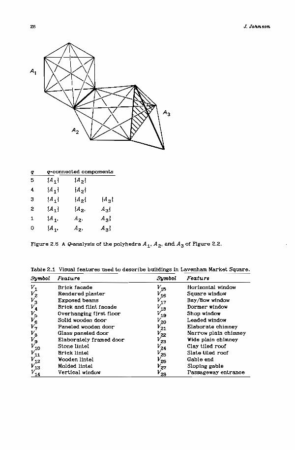
Z6 J. Joh:n.son

q q-connected compoments

5 fAll fAzl4 !A1 l !Azl3 fAll !Azl !A3 12 !A 1 1 !A z, A31

1 fA 1 •Az, A31

0 !A 1-A

z_

A31

Figure 2.6 A Q-analysis of the polyhedra A l' A z- and A 3 of Figure 2.2.

Table 2.1 Visual features used to describe buildings in Lavenham Market Square.

Symbol Feature Symbol Feature

V1 Brick facade V15 Horizontal windowVz Rendered plaster V16 Square windowV3 Exposed beams V17 Bay/Bow windowV4 Brick and flint facade V1a Dormer windowV5 Overhanging first floor V19 Shop windowVB Solid wooden door V ZO Leaded windowV7 Paneled wooden door VZ1 Elaborate chimneyVa Glass paneled door Vzz Narrow plain chimneyV9 Elaborately framed door V23 Wide plain chimneyV10 Stone lintel VZ4 Clay tiled roofV11 Brick lintel V25 Slate tiled roofVlZ Wooden lintel V26 Gable endV13 Molded lintel V27 Sloping gableV14 Vertical window Vza Passageway entrance

A Theory o/Sta.rs 10ft CompLex Systems

•-. I) .

.1, 'h· .,:" ..:

LavenhamMarket Square

Figure 2.7 Lavenham Market Square.

~BI~ Feet 100

I

Table 2.2 The visual polyhedra of some of Lavenham's buildings [the nota­tion a(B1) means building B 1 considered as a polyhedra).

Pblyherlra Visual features

a(B1) <Vz. V5. Vr. ViZ' V14. V15. V16. Vir> V1B. Vzo . VZ4 >

a(Bz) <Vi> Vr. Vii' V15>V16. Vir. V24 . Vzr>

a(B3) <Vi> Vr. Vii' V15. V16. Vir' V19. Vzo' VZZ' VZ4' Vzr >a(B4) <Vi> Vr. Vi0. V14. VZ3' VZ5>Vzr >

a(B5) <Vz· V3· V6. VB> ViZ' V15. Vir' V19. VZ1 >VZ4>VZ6 >

28 J. Joh.nson

•ilJI'iI't ~~ II I

,...~

11 1 ;11111

111,1 1 !/

~X

'l<'X~o--..=::=- - - --======'"-0---==-=-=

=- .-==

(a) (b)

Figure 2.8 Structure versus cluster: (a) Tudor house and (b) Tudor house?

considered to be polyhedra made up of their visual features, as illustrated inTable 2.2. A Q-analysis of the buildings has a major component ~B1S' B 6• Bu. B l .B 13, B 14. Bsl at q = 6. and IBls• B 6• B 1Z. B l , B 13 , B 14 , B s , B 3• B z . B g• B u ' B 16.B a, B7l at q = 5. The first of these contains buildings which conform to the popu­lar concept of a Tudor house, while the Tudor features in the second componentare somewhat more sparse. This example shows that the general concept of aTudor house and what is actually a Tudor house can be different: in terms ofappearance houses built in Tudor times have often been modified according to theneeds and customs of later generations. Thus, at any time the visual structure of atown is evolving towards a new visual structure.

It would be misguided at this stage to consider Q-analysis as just anotherclustering algorithm. Figure 2.8 shows two identical sets of visual features, butclearly 2.8(b) could not be considered a Tudor facade or, indeed, any kind offacade. To resolve this problem more structure is necessary, namely a kind ofgrammar of shapes (c/.. Stiny, 1980) to combine the Tudor features properly.

Example 2.2 Here we consider the structure of tessellated space in remote sens­ing. In a square tessellation let square s be >"-related to square s' if they share anedge or a corner. Then every square is 5-near the squares to its right. left, above,

-.. _,

·•·s s' ···

--~II

_.-'

Figure 2.9 The squares sand s' are 5-near (that is,they share a 5-dimensional polyhedral face).

A Theory o/Sta.rs tn CompLez Systems 29

and below (Figure 2.9), and it is possible to show that the tessellated plane iseverywhere 5-connected. However, Figure 2.10 shows that the tessellated plane isalso everywhere full of 5-holes because diagonally adjacent squares are only 3­near each other.

51 52

53 54

5-near

Figure 2.10 The t.essellat.ed plane is everywhere full of 5-holes (s 1 and s 3 are only 3­near, as are s2 and s 4)'

An Introduction to the Theory of Stars

Whereas q-nearness is defined by the intersection of two polyhedra, the con­cept can be extended to the intersection of many polyhedra. In Figure 2.11(a)there are six tetrahedra which share a common triangle (shaded). These tetra­hedra can be brought together at the triangle to form a star structure, as shownin Figure 2.11(b). The common triangle is called the hub of the star.

Example 2.3 Recall from Figure 2.1 the crosshatching of squares by lines of dif­ferent slopes. Figure 2.12 shows one hundred and seventeen squares, each relatedto four of the eight crosshatch line types. Close inspection of the squares showsthat each of their polyhedra has the face < (J, 7, c5 > or the face < e, ~, T) >, butno polyhedron has both these triangles as a face. Thus the squares, viewed aspolyhedra. define two distinct stars, as shown in Figure 2.13. These stars can beused to partition the squares according to the star they belong to, which revealsthe substructures shown in Figure 2.14. In this particular case the star structureis exactly relevant to the process of pattern recognition.

The concepts of star and hub can be made more precise as follows. Given anypolyhedron u in a simplicial complex KA (B ,X), let the Galois star of u, denotedstar(u), be the set of polyhedra a(a t ) which have a as a face. The Galois starthus defined is a special case of the concept of star in topology, which not onlycontains those polyhedra having u as a face, but also those polyhedra sharing one

30

(a)

(b)

J. Joh.nson

Figure 2.11 (a) Six tetrahedra share a common triangle and so (b) combine to form astar structure with the common triangle as a hub.

or more vertices with a. In this chapter the term star means only the Galois stardefined here. Given any set of polyhedra !a(a 1), a(a z) .... l, let its hub be thepolyhedron which is the intersection of the a(a1.)' Then it can be shown that a isa face of hub[star(a)] and in the special case that a = hub[star(a)J. thepolyhedron a is called a maximal hub. It can also be shown that! a(a 1)' a(a z).··· lis a subset of star[hub({ a(a 1)' a(a z) .... j)], and in the special case that!a(a 1), a(a z),··· l = star[hub<! a(a 1)' a(a z)"" m, the set of polyhedra is called amaximal staT.

Stars and hubs have a number of interesting mathematical properties. butthe most i.mportant is that in Proposition 2.1.

A Theory o/Sta.rs tn CompLe:r Systems 31

Figure 2.12 Squares crosshat.ched by four of t.he eight. lines wit.h different. slopes(ex - ").

11

(a) (b)

Figure 2.13 Stars formed by (a) (J -., - «5 polyhedra and (b) e - <- - "1 polyhedra.

Proposition 2.1!a(a i ). a(az)•... I is a maximal star with hub < b i . b z•... > in FA (B.A) if andonly if (a(b i ). a(b z).... I is a maximal star with hub < ai' a z.... > inFB (A.A-1).

3Z

(a)

J. Joh.nson

(b)

Figure 2.14 A pat.t.ern recognized by t.he star st.ruct.ure of t.he squares. (a) Squares be­longing t.o t.he e - ( - 17 st.ar and (b) squares belonging t.o t.he fJ - '1 - 6 star.

For the proof of Proposition 2.1, see Johnson (1983b, p 461).In Q-analysis, two simplices are defined to be q-near if and only if they have

a common q-face; that is, they share more than q vertices. Two simplices are q­connected if and only if there is a chain of pairwise, q-near simplices betweenthem. Thus, q-connectivity is an equivalence relation on a complex and partitionsits simplices into q-connected components and a Q-a,nalysis lists these com­ponents for each value of q. Since the hub of a set of simplices is itse~f a simplex,let the dimension of a hub be its dimension as a simplex. To maintain numericalcompatibility, let the codimension of a hub be defined as the number of namedsimplices in its star, minus one [in the case that two named simplices are identical,for example, a(a1) = a(az), then each counts separately]. Let a simplex bedefined as an n-q-simplex if its codimension is n and its dimension is q, and let aset of simplices be n-q-near if they an share an n-q-simplex.

Proposition 2.2q-nearness in Q-analysis is the special case of n-q-nearness, for n =1.

Ii'I

A Theory o/Stars in CompLez Systems 33

Proposition 2.3q-connectivity in Q-analysis is the special case of n-q-connectivity, forn = 1, defined as the transitive closure of n-q-nearness.

The literature on Q-analysis concentrates on these restrictions, but Prop­ositions 2.2 and 2.3 suggest that the Q-analysis algorithm can be extended tostructures beyond those defined by q-nearness. However, they highlight a prob­lem which is not apparent in the literature. Q-analysis claims to be a language ofstructure, but all structure analyzed through the Q-analysis algorithm is second­ary to the q -nearness function. However, the Q-analysis algorithm is but a partof the methodology of Q-analysis and most applications of Q-analysis require thediscussion to be vertex-specific. In other words, the specific vertices and sim­plices must be considered explicitly, with properties such as dimensions, q­nearness, eccentricity, etc., taking a secondary role as indica-tors.

The star structure developed in this chapter is not secondary to any mea­sure; the stars and hubs simply exist as structures in their own right. We canimpose mappings, such as dimension and codimension, on these structures, butthese are secondary. The same is not true for the q-connected component struc­tures of Q-analysis. which are secondary to the q-nearness mapping.

Example 2.4 Figure 2.15 shows a simplified version of the road system in theEnglish country town of Bedford. As a simple experiment in Q-analysis, a route wasdefined for each through-traffic pair AB, AC ,... ,HA , fA. A route Ri is related to alink L j if the route traverses that link. The roots are polyhedra connected toeach other through shared links, and links are polyhedra connected to each

o

Approx kilometers

L ..

L,

G

Figure 2.15 Major roads in the Bedford system.

34

Table 2.3 Major stars in the Bedford road system (through-traffic only).

Southern bypass west-east

J. Johnscm

<AE,AF.GE,GF,HE,HF,IE,IF><AE,AF.HE,HF,IE,IF><AE,AF.AG,IE,IF,IG>

Southern bypass east-west

<EA,EG,EH,EI,FA,FG,FH,FI><EA,EH,EI,FA,FH,FI><EA,EI,FA,FI,GA,GI>

<-><-><->

<-><-><->

Southern bypassinteracting Z-way

<AE,AF,EA,EI,FA,FI.IE,IF><AE,AF.AG,EA,FA,GA>

A, origin

<AE,AF,AG,AH,AI>

A, destination

<EA,FA,GA,HA,IA>

E, origin and destination

<AE,EA,EH,EI,HE,IE>

B, origin

<BD,BE,BF,BG,BH>

B, origin and destination

<BF,BG,BH,GB,HB>

Band C, origin

<BF,BG,BH,CG,CH>

<-> <l7,L 8,L 9·L 10,L ll><-> <L1·L9·L10·Lll,L12>

<-> <L1·Lll·L12·Lzz·L34·L35>

<-> <L 1.L l1,L 12.L 33.L 48.L 49>

<-> <L6,L7,L8·L9·L10>

<-> <L 3,L 19.L 20,L 56.L 70,L 71>

<-> <L 3.L 15,L 18.L 19·L 20>

<-> <L 3.L 15,L 18.L 72.L 73>

other through shared routes. Figure 2.16 shows those links in the system ofdimension three or more (Johnson, 1984). These data were reanalyzed by a com­puter program searching for stars and the largest star-hub pairs are listed inTable 2.3.

As with the Q-analysis, these stars show the through-traffic stIllcture to bedominated by the informal bypass south of the town, east to west and west to east.and northern origins Band c. Many British towns have a radial pattern similar toBedford, with the problem that many through-traffic routes must pass via. thetown center. which causes severe congestion. It can be seen that Bedford has asignificant substIllcture for the origins-destinations A, E, F, G, H, I through itslinks south of the center. Also, it is interesting to note how A and. to a lesserextent, E dominate this substructure, because they are at the ends of the bypasslinks. Hence many routes to and from A must share many links, to their mutual

I!'I

A Theory ofStars in Compte2: Systems

L"

Figure 2.16 Bedford road system, through traffic links with dimension 3 or more.

35

detriment [disconnected routes perform better (Johnson, 1976)]. This is a pro­perty of the backcloth, which might not be significant if A generated littletraffic. However, this is not the case; A connects Bedford with many towns to itswest and with the M1 motorway, so carrying a large volume of traffic. It isinteresting to note that since the original analysis a formal bypass has beenopened, which extends the informal southern bypass in the west to avoid the diffi­cult urban roads between I and A.

An Introduction to Traffic in Complex Systems

In complex systems one can make a distinction between qualitative data andquantitative data, the first being expressed as relations and the second beingexpressed as numerical functions. The methodology of Q-analysis makes a distinc­tion between a relatively static backcloth structure (qualitative), which supportsa relatively dynamic traffic of system activity (quantitative). Over and above this,the methodology claims that the star structure of the backcloth constrains thebehavior of the traffic - it allows and forbids, but does not require (see Chapter1). To illustrate this, the route-link structure supports a traffic of motor vehiclesand constrains this traffic in the following ways. First, the vehicles cannot travelwhere there is no road: no backcloth implies no traffic. Second, a road may existand allow vehicles to pass, but there may be none: the backcloth allows traffic,but does not require it.

The previous sections suggest that the structure of relations can be investi­gated through their families of polyhedra and the related connectivities. In the

36 J. Joh.nson

IT

----------...... IT(a)

Figure 2.17 TraffIc as a mapping from a polyhedron Lo a number.

---------..... lilT(a,)

~

--------...~ lilT(a2 )

lilT ~--------•• lilT(a3)

FIgure 2.18 IllusLraL10n of q-LransmIssIon: a change 611" on 0"1 Induces a change 611" onO"Z' which Induces a change 611" on 0"3'

first instance, the representation of traffic can be thought of as an arrow map­ping a polyhedron to a number (Figure 2.17). The theory of q-transmission (John­son, 1962a) suggests one method in which backcloth structure can constraintraffic. In its simplest case, we can define change in traffic to be transmittedfrom one polyhedron to another through a shared q-face. For example, Figure 2.18shows three polyhedra with 0"11-near O"z and O"z l-near 0"3' Thus, 0"1 and 0"3 are q­connected, but they do not share any vertices. Under some circumstances, it ispossible that a change in traffic, 611", on 0" induces a change 611" on O"z because theyare l-near. Similarly. the change on 0"2 may induce a change 611" on 0"3 becausethey are l-near. In this way. changes in traffic may be transmitted from onepolyhedron to another. with which it has no shared vertices. via intermediate con­nectivities. Figure 2.19 illustrates this for a simple road system with routesbetween A and C. Band C, and Band D. Suppose there is an accident on link L zwhich restricts its capacity. The resulting traffic flows on L 5 and L 6 decreasebecause fewer vehicles are able to travel AC in unit time. If the road system iscongested it may be that vehicles on route Be are normally slowed by congestionon L 5 and L 6 . A reduction in traffic on AB reduces congestion on links L 5 and L6 •

and hence vehicles on route BC spend less time on L 10, L 9• L 7 • and L 8 . In turn.this reduction in congestion may reduce travel time on route BD. By this argumentreduced flow on AC is l-transmitted as reduced travel time on B::. which is 1­transmit ted as reduced travel time on BD.

A Theory o/Sta.rs o£1l. Comp1e% Systems

B

37

c D

Figure 2.19 Changes t.ransmit.t.ed t.hrough a single road syst.em.

A number of theorems (Johnson, 1976) show that disconnecting the link androute structures enables road systems to perform better. Dramatic examples ofthis occur at complicated road intersections which, in Britain, are often rounda­bouts (called rotaries or traffic circles in North America). For instance, in 1973one of the roundabouts in the town of Hemel Hempstead was causing severecongestion and an experiment was devised which implemented six rnini­roundabouts and two-way flows (Figure 2.20). Intuitively, it is clear that the designbefore the experiment caused many routes to be highly connected and thereforecaused many vehicles to interact with each other, to their mutual detriment. Simi­larly, it is clear that the experiment has caused at least some pairs of routes (e.g.,ab and if) to become disconnected, to their mutual advantage. These intuitionsbecome more difficult when considering the whole intersection. However, the com­puter analysis and theorems show the new design to be significantly disconnectedand that the traffic flow must improve, as, indeed, it has:

The current. experiment. being undertaken at. t.he Plough has, in t.erms ofcapacit.y and reduction of delays, proved a success and a new lease of life hasbeen given t.o t.he junction. (The West Herts Transportation study, Hert.­fordshire Count.ry Council, 1974.)

Vehicular traffic is an example of a much more general idea; for example,Johnson and Wanmali (1981) considered a traffic of retail goods in Indian periodicmarket systems, Gould (1981) considered a traffic of electricity on an unstable

38 J. Johnson

Figure 2.20 Hemel Hempstead system: (a) preexperiment, (b) postexperiment. The post­experiment design significantly disconnects the link and route structure, therebydramatically increasing capacity.

physical backcloth in the US, Gould et al. (1984) considered a traffic of televisionprograms across a world backcloth, Atkin (1977) studied many kinds of trafficassociated with university life, and so on.

Hierarchical structure

As is well known, large complex systems often have hierarchical descriptionsin a hierarchical vocabulary. A common problem when studying such systems isthat the description may be too coarse, with insufficient detail, or too fine, withoverwhelming detail (Figure 2.21). The intermediate word problem involves findinguseful words between too high and too low a hierarchical level. This is illustratedin Figure 2.22, where the purpose is to describe television programs. Manyhierarchical schemes attempt to give exclusive classes, despite real systems hav­ing a natural cover structure with intersections (Figure 2.23). In practice,exclusive classes are not necessary and they violate natural structure in theobservations.

An intermediate word like SPORT has many things aggregated into it, and thisset can be represented in the usual Venn diagram. If this is joined to a pointrepresenting SPORT at a higher level. a cone is formed (Figure 2.24). The conerepresentation can be useful in a number of ways; for example, it gives a graphicillustration of the Non-partition Principle (Figure 2.25) and it illustrates the kindof structural requirements one would probably impose on a hierarchical scheme(Figure 2.26). These cones can also be thought of in a structural way, as illus­trated in Figure 2.27. Here the intermediate words Tudor-l, Tudor-2, and Tudor-3are connected in terms of their lower level structure. It is interesting to askwhere archetypes like TUDOR come from, see Postulates 2.1 and 2.2.

A Theory o/Stars in CompLe:z: Systems 39

The hierarchical soup ­overwhelming detail

What are the

intermediate

words?

Insufficientdetail

ANYTHING(the universe)

EVERYTHING(all minutiae)

Figure 2.21 The int.ermediat.e word problem.

ANYTHING

~f f t~

TffFootball Murder Jazz

Figure 2.22 Part. of a heirarchy for describing t.elevision programs.

FDSIVLATE 2.1 Out of the combinatorially many ways things combine, human beingsselect a relatively small subset to name.

PaSTULATE 2.2 The principle of usefulness; that is, names are given to particularcombinations because it is useful to do so.

For example, the archetype "Scrambled Tudor" did not exist before, but it doesnow because it is pedagogically useful (Figure 2.28).

40

SPORT

7\Ball games Water sport

7\/\

Level N + 2

Level N + 1

J. Joh.n.son

football water polo diving Level N

Figure 2.23 Level (N + 1) covers level N, but it aoes not partition it.

SPORT

Base (SPORT)

Figure 2.24 The hierarchical cone constructionwith apex SPORT and base the Venn diagramof the set of things aggregated to SPORT.

A Th.eory a/Stars in CompLex Systems

Figure 2.25 The Non-partition Principle.

Figure 2.26 The Nested Base Rule Ii! Af'l +1 aggregatesinto A N then base(Af> <; base(A N 1}].

41

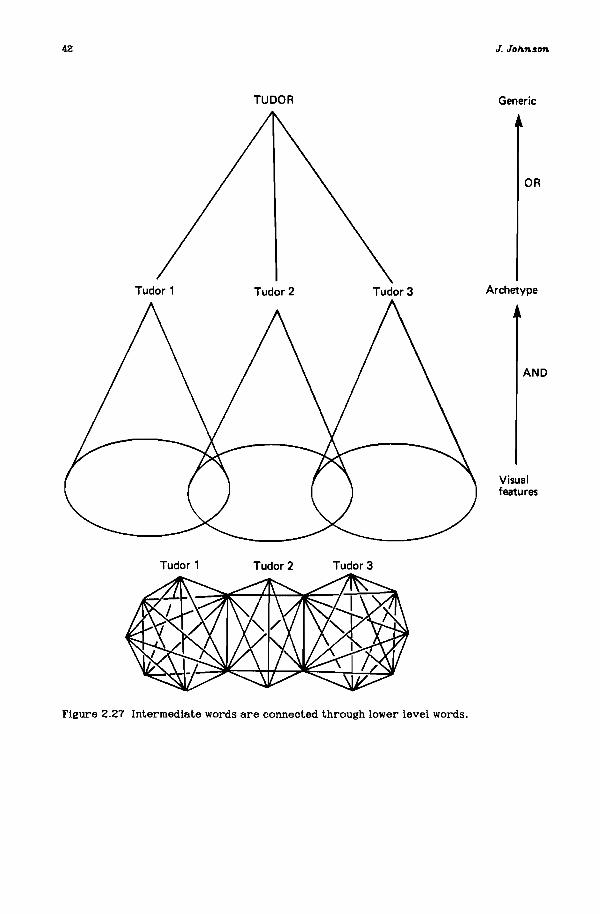
42

TUDOR

J. Joh.nson

Generic

Tudor 1 Tudor 2 Tudor 3

OR

Archetype

AND

Visualfeatures

Tudor 1 Tudor 2 Tudor 3

Figure 2.27 Intermediate words are connected through lower level words.

Ii

A Theory o/Sta.rs in CompLez Systems

-O~

-:=~~-~---

Figure 2.28 Scrambled Tudor house style (compare with Figure 2.8).

43

Example 2.5 Stars and the hierarchical definition of Tudor house style. The rela­tion between Lavenham building facades and visual features contains the stars:

<->

<->

<wooden lintel, horizontal window,square window, leaded window, clay­tiled roof><exposed beams, wooden lintel,square window, leaded window, clay­tiled roof>

which identify sets of houses that are definitely Tudor in style. It is interesting tonote that B 1 in the first does not have the feature of exposed beams in its facade;the beams are doubtless present in the Tudor construction, but they are con­cealed by plaster rendering and white paint.

The following stars are also associated with a Tudor-style house:

<B1 , B 12, B 13 , B 14,B15 >

< B 5 , B 6 , B 12, B 13 , B 15 >

<->

<->

<->

<->

<->

<wooden lintel, horizontal window,square window, leaded window, clay­tiled roof><first floor overhang, wooden lintel,square window, leaded window, clay­tiled roof><wooden lintel, vertical window,square window, leaded window, clay­tiled roof><wooden lintel, square window, leadedwindow, clay-tiled roof><exposed beams, wooden lintel, hor­izontal window, clay-tiled roof>

44 J. Joh.nson

The following stars are interesting because they contain anomalies in terms of adefinition of Tudor style:

<B 3 • B 6 , B 12• B 13, B 15 >

<B 1 , B z' B 3 , B 6 , B 15 >

<->

<->

<horizontal window, square window.leaded window. clay-tiled roof><paneled wooden door, horizontalwindow. square window, clay-tiledroof>

In the first of these, B 3 is included amoung the Tudor houses. although it appearsVictorian at first sight. In this case the leaded windows are definitely of a laterVictorian or Edwardian style which means they, at least, do not date back to Tudortimes: perhaps the descriptor leaded window requires further clarification?Another anomaly with this house is its clay-tiled roof, while the construction of itssloping gables is very similar to the Victorian cottage next door. For economic rea­sons, most Victorian houses have slate roofs, but this one has a clay-tiled roof.Perhaps it has been reroofed since Victorian times with clay tiles, or was it builtusing old clay tiles from another building?

The second star contains a mixture of Victorian and Tudor house styles. sosimilar considerations to the previous case apply. Now we have Tudor buildings fit­ted with paneled doors more characteristic of later times; again, one can speculatethat old doors have been replaced with new.

These anomalies show that house styles exist which are hybrid, neitheracceptably Tudor nor obviously Victorian. As noted before, the visual structure ofan area evolves over time as one generation after another effects repairs andimprovements. It is interesting to note that the anomalies are seldom named andthat people very often restore old properties, which involves removing visuallyincongruous features and replacing them with others more original. It may be thatinitially we name combinations of features somewhat arbitrarily, but it would seemthat once something has been recognized and named there are strong pressures tomake similar objects conform to the name.

The problem of hierarchical set definition, or classification, involves discrim­inating things which are different and aggregating things which are similar (John­son, 19B1c). Clearly, stars tell us which things are similar and are potentially veryuseful in this. However, a binary relation between, say, facades and features is notsufficient to discriminate Tudor from scrambled Tudor, because these stylesinvolve relations between the elements in the facade: Georgian style windows arearranged in vertical and horizonal rows, roofs are on top, and so on. In otherwords, there is a complicated set of rules which fit all the parts together prop­erly. Such rules can be thought of as compound propositions which take the valuetrue when things fit together properly and false when they do not. In fact. thepropositions can be subdivided in such a way that testing any of the subproposi­tions as true is sufficient to show that the compound proposition is true; the sub­propositions are linked by the conjunction OR. Furthermore, each subpropositionis a set of simple propositions involving only the conjunction AND. Any single oneof the subpropositions is effectively a set of rules to establish whether a given setof features combines properly for aggregation. Clearly. a necessary condition forthis is that the building possesses all the relevant features - that is, it has thecorrect star structure.

Ii

A Theory o/Sta.rs in Compl£:Z: Systems

Propositions and relations are effectively the same things: one saysa l • az•....a n are R-related if and only if P(a l • az•...• a n ) = true. where P definesR. This allows the definition of different polyhedra to those given by a binaryrelation: let <al' az•...•a n > be a polyhedron if and only if P(al' az•....a n ) = true.

In the case of visual features and buildings it is possible to obtain two dif­ferent sets of polyhedra: the first by observing the relation A between buildingfacades and features: the second by defining a set of propositions which testwhether a given set of features aggregates to a recognized type. By definition.the aggregation propositions can only be applied if the necessary set of verticesis present; that is. is a face of the A-polyhedron. Thus. the polyhedral analysisbecomes a necessary part of the aggregation procedure and also has considerableheuristic value in eliciting appropriate aggregation propositions. The relationalpart of an aggregation applies to what has been called the AND aggregation;archetypes are aggregated by a simple OR (Johnson. 1983a). This is illustrated inFigure 2.29.

TUDOR

/

'"

/

/

OR-aggregation

AN D-aggregation

\

\\

\

\\ ,

... ,A "

I, A'

Building ooc------ --- -­facade.. ~

\ ,... ...

" " " ....Visualfeatures

Figure 2.29 Hierarchical aggregation through AND and OR aggregations.

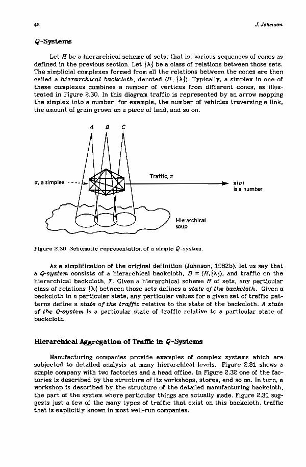
46

Q-Systems

J. Joh.nson

Let H be a hierarchical scheme of sets; that is, various sequences of cones asdefined in the previous section. Let p\j be a class of relations between those sets.The simplicial complexes formed from all the relations between the cones are thencalled a hierarchical backcloth, denoted (H, PloD. Typically, a simplex in one ofthese complexes combines a number of vertices from different cones, as illus­trated in Figure 2.30. In this diagram traffic is represented by an arrow mappingthe simplex into a number; for example, the number of vehicles traversing a link,the amount of grain grown on a piece of land, and so on.

A 8 c

Traffic,1T

Hierarchicalsoup

1T(a)is a number

Figure 2.30 Schematic representation of a simple Q-system.

As a simplification of the original definition (Johnson, 1982b), let us say thata Q-svstem consists of a hierarchical backcloth, B = (H, PloD. and traffic on thehierarchical backcloth, T. Given a hierarchical scheme H of sets, any particularclass of relations p\j between those sets defines a state of the backcloth. Given abackcloth in a particular state, any particular values for a given set of traffic pat­terns define a state of the traffic relative to the state of the backcloth. A stateof the Q-system is a particular state of traffic relative to a particular state ofbackcloth.

Hierarchical Aggregation of Traffic in Q-Systems

Manufacturing companies provide examples of complex systems which aresubjected to detailed analysis at many hierarchical levels. Figure 2.31 shows asimple company with two factories and a head office. In Figure 2.32 one of the fac­tories is described by the structure of its workshops, stores. and so on. In turn, aworkshop is described by the structure of the detailed manufacturing backcloth,the part of the system where particular things are actually made. Figure 2.31 sug­gests just a few of the many types of traffic that exist on this backcloth. trafficthat is explicitly known in most well-run companies.

A Th.eory ofSta.rs 1.n Compte:!: Systems 47

<The company>

expenditure~_---_...:..._-----_.$e

r income------.;....;.;;..;..;.;...-----....~ $i'-- profits I $p

Profits «The company» = Income «The company» - Expenditure «The company»

(a)

material consumed

______.....;.ma;.;.;;.;t;.;;e.;.;ri~a;..'~un;.;.i;.;;t..;;co;.;;.;;.st;;....__ $r(q' + q)

material consumed_------------....~ q'tonnes~ expenditure~ • $e'- wages • $w'

"--- overheads • $0'

:

q tonnes

L::-- expenditure---..;.;.;.:;..;;.;,;,;;;.;,;,;;;.;..;;...----... $e---_______w_a""g_es.....;. .~ $w

'-- overheads .. $0Manchesterfactory

Londonheadoffice

Expenditure «Bristol factory» = $w' + $0' + $[q' X r(q' + q)]Expenditure «Manchester factory» = $w + $0 + $[q X r(q' + q)]

(b)

Figure 2.31 Two relatively highly aggregate descriptions of a company, (a) more hIghlyso than (b).

Without laboring the point, Figure 2.31(b) shows that some traffic must referto more than one vertex of a polyhedron. It is clear that the unit cost of materialto ea.ch factory depends on the quantities required by both factories, since in thiskind of system unit costs usually decrease with quantity. Also, unit costs and quan­tities are usually step functions with discontinuous changes in price - even simplesystems are unlikely to be linear, or even continuous, in their traffic.

Figure 2.32 shows how the company can be described in increasing detaildown to the level of the machines used and specific articles manufactured.Although academics tend to dislike such a detailed level of description. it isinteresting to note that those responsible for complex systems. such as themanagement of a company. do. indeed, have long lists of the parts used. do knowprecisely who is employed and how much they are paid, do know how manymachines are owned and where they are, and so on. It is clear that without thisinformation the company would be unmanageable.

48

MANCHESTERFACTORY

J. Joh.nson

Stores ---

Office 6

Value of stock----------------------------_ $v

overheads_---..;..;.;.;.;.;=;;.;;,..------. $0r- material consumedWorkshop 7 • $q

'--- lathe operators---------------.~ n men

(a)

WORKSHOP 7

Lathe 4

Mn12~part D411796

~__---"'----------... d parts~ maintenance costLathe 1 • $w"""---.. ..:o..:;:p..:e;.;ra;.;t..;.o;..r..;.co,;.,st:..:..:..s • $m

(b)

Figure 2.32 Two relatively disaggregate descriptions of parts of a company. (b) more sot.han (a).

This hierarchical view of complex systems highligh ts a number of aspectsthat many analysts prefer to overlook. The most important of these is the natureof the aggregation of traffic (Johnson, 1983c) and the implications of this forpredicting future system states. Figure 2.33 is an abstraction of a system at, say.levels N + 5, N + 4. and N + 3. corresponding to a complicated organization. Letus assume the backcloth for the analysis and consider the traffic. Between level

Ii

A ThI!ory 0/Stars in Compl.ez Systems 49

N + 4 and level N + 5 the question of hierarchical aggregation may resolve itselfin terms of a function. with y =/ (% l' % 2" "'%n)' In real systems this function isprobably quite complicated, almost certainly piecewise discontinuous at manyplaces. possibly multiple-valued, depending on the system's history, and so on.Note that the expression y =1 (% l' % 2' ...• %n) almost certainly does not meany =/1(%1) +12(%2) + ... +In(%n)' except for the simplest systems, and that/ (% l' % 2'···.%n) is a function of the whole polyhedron.

Level N + 5 • ---------------------- Y Numbers

h ?

Numbers

?

Level N + 3

----------/----:.'\-----'-~ xl

G \ _x2

Level N + 4 -7 I - x3

--------1------7,----- X 4

-------:----\----7+----... Xs---------i----\.---~-----I_~ Xs

ht

/

\\

7

:-.. Numbers

..-..Figure 2.33 How does traffic aggregate relative to the backcloth?

Descending the hierarchy from level N + 4 to level N + 3 the backclothitself is more complicated - the N + 4 vertices now become N + 3 polyhedra withassociated discontinuities between some of the polyhedra. Recall that trafficbehavior depends on the star structure of the backcloth in some systems: how are

50 J. Joh.nson

these more subtle properties of the traffic aggregated? As drawn in Figure 2.33the variable %5 may depend on a combination of traffic functions defined on anumber of N + 3 level polyhedra. It is then likely that the aggregation is condi­tional on both the value of the N + 3 traffic and its supporting star structure.

Finally, one can ask how the traffic on a complex hierarchical systemis sometimes required to sustain the system. In some cases the maintenance ofrelations may consume money; for example, the backcloth that supports telecom­munications traffic also consumes income traffic - to the extent that the leastexpensive backcloth necessary to support the communication traffic is sought:telephone, telex, electronic mail, dispatch rider, etc. In other cases incometraffic is invested in creating new backcloth structures - a new factory, a newmachine, a new employee, for example. The decision to make such investmentreflects an awareness of the managers at N + 5 that $p is, indeed, determined bystructure at lower levels in the system. Since complex systems are complex theseexamples can only hint at the application of Q-system theory to real cases. How­ever, an important point remains to be made in criticism of the kind of analysisfrequently involved in the prediction of future system states of nations, interna­tional groupings, or even the world.

Figure 2.34 shows some typical variables involved in the equation of unem­ployment for Britain. Some analysts seek functional relationships between suchvariables and provide predictions on this basis. Despite such predictions beingnotoriously unreliable, there is little evidence of these analysts asking fundamen­tal questions about the methods they use: indeed, some do not even admit thatthey deliberately shut their eyes to the real system because it is too complicated.Complex systems are undeniably complicated in the numbers of elements, rela­tions, and functions they involve. This complexity involves the intimate relation­ship between traffic and stars (at least); and that complex systems are invariablyhierarchical with complicated hierarchical relations on the backcloth and traffic.Given this, a main argument in this chapter is that one will not understand com­plex systems by ignoring everything but highly aggregate numerical relationships.

People employed

?= People unemployed :F.T. Index

numbersBRITAIN --- Bankruptcies last month

~New businesses last month

Etc.

Mean income«BRITAIN>1 = '(People employed, ... )

Figure 2.34 An adequate description of a complex system?

A Theory o/Sta.rs tn CompLex Systems

An Appropriate Concept of Time for DescribingChange in Complex Systems

51

Time is implicit in our interest in systems, but too often an inappropriateNewtonian concept of time is used. Consider the pendulum in Figure 2.35 which isused to measure clock time. Suppose an observer can detect the presence orabsence of the pendulum bob at point p , and counts aloud the number of times thepresence of the bob changes to the absence of the bob at p. When the pendulumis swinging one would hear the observer saying "one, two, three, ... ", which can beused to construct a sequence of now-moments: now-l means the observer says"one", now-2 means the observer says "two", and so on. This sequence of now­moments tnow-l, now-2, now-3, ... I is totally ordered and has the usual propertiesof Newtonian time. Note that it is not the position of the bob which marks time, itis the change in position; the stationary pendulum bob cannot be used to marktime in this way.

\ ," " " ...

- - --p p

(a) (b)

Figure 2.35 The pendulum used for measuring clock time: (a) moving and (b) stal1onary.

In physics the now-moments are mapped to numbers according to theirsequential occurrence and, by a further process of abstraction, it is assumed thatsubtracting one of these numbers from another gives an appropriate measure ofduration. This view of clock time is supported by the observation that differentphysical systems give consistent durations when compared. For example, pendulumclocks, spring clocks, water clocks, candle clocks, quartz clocks, etc. all givemore-or-less coincident now-moments signifying the passing of, for example. anhour. However, these clocks have to be calibrated against each other, there beingno absolute duration. Similarly, some clocks are internally more consistent thanothers, which we interpret as being the ability to measure time more accurately.However. it can be argued that clocks do not measure time. they define time rela­tive to their now-moments. In classical physics, motion and change in motion areused to observe (pendulum) clock time in the first place; then time is subsequentlyused to define and observe motion as velocity, acceleration, etc. In other words.motion is tautologically defined by motion, or time is tautologically defined bytime, in physical systems.

The now-moments of the pendulum clock are particularly simple, with onlytwo observable states; namely, the bob is at p, and the bob is not at p. Thus the

52 J. Joh.nson

now-moments oJ a physical system can only be observed as changes in stateoJ the system.

The discrepancy between physical time and social time is well known (e.g.,Sorokin and Merton. 1937); time flies, time drags. and so on. This is sometimesinterpreted that the social system is in some way out of step with true (clock)time. However. it is equally possible to say that clock time may not be appropriatefor measuring time in social systems. Certainly, social events do not appear to betotally independent of clock time, since many human activities are defined interms of days, weeks. months. years. etc. On the other hand. historians measuresocial time by social events such as wars, treaties. births. deaths, marriages.inventions. and so on. Although they find it useful to associate such events withdates in clock time. there is seldom the suggestion that the cycles of history canbe related to exact clock-time durations.

Social events are characterized by structure; they are made up of manynecessary parts which must be combined in the correct way for the event to havehappened. Events have the property that the whole is more than the sum of theparts. For example. consider the event Workshop on Structure and Evolution ofSystems. Somewhat simplistically. suppose it is made up of the activities <travelfrom home to Abisko>, <listen to papers>. <academic discussion>. <social discus­sion>. <contemplate nature>. and <skiing>. The academic event is characterizedby <travel from home to Abisko. listen to papers. academic discussion>. presum­ably to be experienced by all participants. with all parts necessary for the eventto have happened. However. most experience a richer event: <travel to Abisko,listen to papers. academic discussion, social discussion. skiing> for the gregarioussportsperson; <travel to Abisko, listen to papers, academic discussion. contem­plate nature> for the introvert, and so on. For each of the participants, the partsof the event form by themselves or with others (evolve?) until the event is recog­nized to have happened. Some have a feeling that the event develops over a clocktime week, others may feel everything gels on the last day. In either case. it islikely that the event of participating in the workshop marks in their memory whenMay 19B4 occurred. rather than vice-versa.

Atkin has described such processes as p-events. where the number preflects the number of parts of the event (Atkin. 1974. 1977, 19B1). These p­events reflect the observation that something has changed in the system. In justthe same way that changes in the physical system of the pendulum seem to beappropriate for defining physical clock time, it does not seem unreasonable to letchanges in social systems define social time. In other words. it is suggested thatthe time appropriate to a Q-system is defined by changes in state of the Q­system. In a Q-system the past can be defined to be all states of the systemwhich have been observed, excluding the state of the system as it is beingobserved now in the present. The Juture can be defined to be all possiblestates of the Q-system and, of the many possible states in the future, only somewill be observed. A discussion of past. present, and future in logic can be found inPrior (1967). If one accepts that a Q-system can have a single state. s. at a givennow-moment (effectively a definition of now-moment), it is possible to produce akind of stochastic lattice (Figure 2.36) which corresponds to what Atkin (1979) hascalled the NOW-horizon. Let a path through this lattice be called a Q-systemtrajectory through social time. In other words, a Q-system trajectory is a set ofQ-system states !sl, ....s'" l. where s1. +1 can follow s1..

Ii

A Theory o/Stars tl'l. Compl.e:z: Systems 53

$41

/$31 II

/ ~$42

$21 - //' ----.. $32 II'

--......$1 II $44

~/

$33 ....

------ ~$22 ...

~$46

/$34 II'---.

$48

Figure 2.36 A slochaslic laltice of Q-syslem slales.

It is possible to consider Q-system trajectories as p-events which grow assuperevents of previous events [Figure 2.37(a)], where the Q-system does not "for­get" its past. However. there are many Q-systems in which earlier p-events' arelost by accident or design [Figure 2.37(b)]; for example, the erection of scaffold­ing in the construction of a building is an event which is subsequently removed asa means to the event "the building is finished". Thus, some system trajectories aredevelopments of events from events which have ceased to exist.

Figure 2.37 The developmenl of evenls from previous evenls (p-simplices arerepresenled by polygons): (a) p-evenls as superevenls of previous evenls which slillexisl; (b) lhe developmenl of evenls from previous evenls which have ceased lo exisl(evenls E l' E z. E 3 , and E 4 cease lo exisl as E 5 evolves).

54 J. Joh:nson

..(al

Figure 2.38 Changes in state determined by changes in traffic: (a) p-events as changesin traffic (p-forces); (b) changes 611" can be predicted to arrive at (7 at now-moment n(changes are q-transmitted through the fronts Fo ' F1 •...•Fn ).

In some cases. the trajectories are characterized by changes in the trafficstate without any change in the backcloth state (Figure 2.38). For example, thebackcloth to the pendulum does not change with counting the passing of now­moments and their related intervals. The theory of q-transmission (Johnson.19B2a) examines the change of traffic values over a backcloth, the general ideabeing that q-dimensional changes (q-forces) are transmitted down q­connectivities. It transpires that simplicial complexes have a transmission frontstructure which relates to the time it takes for changes to occur in the traffic.Given a q-connectivity. one might ask when a q-force at one end is q-transmitted

A Thllory ofStars in Compte% Systems 55

to the other. The answer can be given precisely as the number of transmissionfronts along the chain, which gives the tautological prediction that a q-force (achange in q-dimensional traffic) arrives at a simplex precisely at the moment itarrives [Figure 2.38(b)].

Time and Prediction in Complex Systems

Suppose every social Q-system exists in a single state when observed at anygiven clock time and that Q-systems are not observed and recorded continuouslyin clock time. The history of a social Q-system is then composed of a series ofclock-time defined states, st. In general, let the expression Os = s t! _ S t 1

represent the change of state between clock times t 1 and t 2'

The relationship between social and clock time can be schematically drawn asin Figure 2.39, in which the polygons represent simplices that are associated withchange as events. Implicit in this picture is a large amount of omitted backcloththat does not change with these events and, for simplicity, it is assumed the

events are not simultaneous. Thus, the transition from system state s t 1 to state

s t! is schematically represented by a hexagon (5-simplex) changing to an octagon(7-simplex), this change happening between clock times t 1 and t 2' If it is now t 3'

all the past events can be ordered in retrospective clock time (it is assumed),

0 0 0o 00\

----. Past ------.... Now -----..... Future

Figure 2.39 Mapping social time into clock time (Q-system events are represented aspolygons),

56 J. Johnson

but it is not always possible a priori to predict whether other events will occurbefore or after each other in future clock time. Thus, we can know what the pos­sible system states are, but we may be unable to reliably predict which will occurfirst.

In his book Multidimensional Man, Atkin (1981) speculates on some veryinteresting relationships between the dimensions of events and clock time anduses the formula (Atkin, 1978, p 292)

Pt1[p +Z) x [t +1)t=l t +1 lz

as the time ratio of structural interval to Newtonian interval to derive the rela­tionships below. Notice

is the number of t-faces of a (p + l)-simplex and the number of edges in each t­face is

Atkin also assumes hierarchically unbound time-intervals of successive B-events atsuccessive levels, with 24 h taken as a given fact. Although Atkin does not argue aprecise relationship between social time and clock time, his point that high­hierarchical, high-dimensional social events take a relatively long clock time tooccur is very convincing; for example he gives relationships between humanevents and clock time (Atkin 19B1, p 196):

Waking/sleeping LifeQuickest impression

1.34 x 10-4 s

Breath

3.4s 24h 70y

There is no doubt that many human activities relate closely to clock time andthe related physical events. Attempts to ignore clock time when traveling canresult in the social-psychic-physical disorder called jet lag; the period of gesta­tion for humans is about nine calendar months; it takes three years of study toobtain a bachelor's degree at some universities, and so on. Some of thesecorrespondences reflect biophysical properties which genuinely occur in clocktime and others are conventions which apparently depend on social considera­tions.

POSTULATE 2.3 Prediction hypotheses:(1) Some social events, for example birthdays, can be tautologically predicted in

clock time. These predictions are exact.(2) Some social events, for example gestation and birth, can be predicted in

clock time (inexactly), because physical processes are involved.(3) Some social events, for example football matches and television watching, can

be predicted in clock time because they have been planned to occur at

Ii

A TheoT1/ olSta.rs tn Compte:z: Systems 57

specific clock times. These (exact) predictions may become incorrect forother socially determined reasons and events.

(4) Some social events can be predicted in clock time on the basis of previousobservations; for example, taking an annual holiday. These predictions maybe inaccurate or incorrect.

(5) Some social events predictably must precede other events; for example, theroad must be built before people can drive along it.

(6) Some social events can be seen retrospectively as predictable from previousevents, but systematic collection of data about those previous events wouldbe impractical, for example: the car broke down; I walked home; it was fine; Iwent the long way round; I heard a bird; I looked up; I tripped; I broke myleg; I am not at work, ... the car breaking down caused me to be absent fromwork.

(7) Some events can be tautologically predicted in social time; for example, whenI am good enough I will play in the first team; when I feel better I will get outof bed.

(8) Some events seem chaotic with respect to clock time; for example, whether Iwin or lose when playing dominoes.

This can be summarized as follows: there are (at least) two types of time: they aremeasured by physical events (clock time) and social events (social time); theseevents are determined by changes in the state of physical or social Q-systems;social time can be precisely associated with clock time for past and presentevents; some social events can be precisely predicted in clock time; some socialevents can be roughly predicted in clock time; and some social events are notpredictable in clock time beyond the possibility that they might happen.

The speculations which attempt to relate future states of Q-systems to clocktime have one of the forms:

(1) The Q-system will have the state st at some unknown i, i > now.(2) The Q-system will have the states stand s1, and the former precedes the

latter in clock time.(3) The Q-system will have the state s t after some t min in clock time, where

t min < i.(4) The Q-system will have the state s t before some t max in clock time, where

t max > i.

If an event must occur before a system state s1 occurs in clock time andafter a system state st occurs in clock time, then [st, s1] is defined to be a crsystem window for that event. If it is speculated that an event will occur beforea clock time t max and after a clock time t min' then [t min' t max] is defined to be aclock-time window for that event. For example [the universe at your birth, theuniverse at your death] is a Q-system window for the event of you reading thischapter. More speculatively, [1984 AD, 2084 AD] is a clock-time window for theevent of you telling me what you think of it.

58 J. Johnson

When planners and decision makers are attempting to locate socia1 events inclock time, it will probably be helpful if (as far as possible) they arrange theirgoals (desired states of the Q-system) into:

(1) Those with time window [now, t mwel(2) Those with time window [t min' t max].(3) Those with time window [t min' ?].(4) Those with time window [now, ?].

Here t min and t max exist in clock time. The first three of these relate goals toclock time and the last states that the goals belong to the unknown clock-timefuture including, for practical purposes, never happening.

In principle. the time windows for a set of goals can be superimposed on eachother, as illustrated in Figure 2.40. With any set of goals. the intersection of theirtime windows is either empty or a subwindow in clock time. Let W be the set of allsubwindows that can be generated by the time windows for a set of goals G. Thenit is an interesting research question to ask: Does the structure of the relationbetween a set of goals G and a set of time windows W have any (heuristic) value forstrategic planning in clock time? Certainly the complex KG (W ,ft.) shows how the

.!-9I e lO

..!:.lL __ __ .. _.. _

(b)

Ie)

e51-....:::....---- ... ---- ..... ------ ... -- .... -----ee

e7e8,........:=---_ -- ------ -----

t min1

tmin3 ~12 - - - - - - .. - - . - - - - - - -. _.. - - - ?e13 .

--- -- - . -- .. _. -- -'. 7

tmin4-----~1~ -- - , -- -- - .. 7_____ ~ 1.5.. __ . _ ___ . _.. _. . .. . ?

tm...,.in-5-----:.1~-- ---- -- -- -- "'" - 7.17._ _ _ _.. _._ __ .. 7

Now

e18

{1----------:.:::....---------------7

(d) e19 7

7

Figure 2.40 Juxtaposition of time windows for future events, e1. . where the lime windowsare (a) [now, t max]; (b) [t min. t max]' (c) [t min,?], and (d) [now,?].

Ii

Social events not knowna priori to be before orafter each other in clock time.

A Th.eory o/Sta.rs in Comptez Systems

oo

o

59

Before ....__------------------------.....~ After

Figure 2.41 Quasi-ordered events in social time.

goals are related to each other through shared subwindows of clock time. Also, thecomplex Kw(a.'A -1) shows how intervals of clock time are related to each otherthrough shared goals.

The subintervals not containing other subintervals can be ordered by clock­time occurrence. wi occurring before wi +1. Let at be the set of goals that canoccur in time window w t E: W. Then the expression

1'1.

II at,t =1

the Cartesian product of the sets at. contains all those Q-system trajectorieswhich begin with a goal that can occur in w 1 and end with a goal that can occur inw n . where w1 • w 2 •...• w n have no subintervals. These trajectories could be writ­ten (all' ale .....al;. ), where ali E: a1 ; that is, the Q-system is steered toward the

goal a:;. via a set of desired system states which are, by definition. themselves

goals. Theoretically, decision makers could devise tactical sets of actions toproceed from one goal to another in a Q-system trajectory.

However. those goals which will occur a long while into the clock-time futuremay be possible in very many clock-time subwindows. Thus, the further ahead thatis planned, the more possible system states that have to be considered for tacticalplanning. Clearly, tactical planning should not be attempted beyond the ability tocope with the combinatorial possibilities.

Although events are totally ordered in historical clock time. there seems nogood reason to insist that they are necessarily totally ordered in the future. Forexample. if two events share the same clock-time window, one does not know whichwill occur first. Certainly, there is no suggestion that the events will necessarilyoccur simultaneously. Thus, one can view future events as being quasi-ordered by

60 J. Joh.nson

their occurrence in future time (Figure 2.41). In turn, this means that the stochas­tic lattice of Figure 2.36 must be revised; its vertical columns of system states areimplicitly alternatives for a single future time.

Suppose that decisions about a Q-system are made in a language which canhave a single state of the system as a vertex. Then the political part of makingdecisions consists of O-dimensional traffic on this metastructure, and choosingstrategies (sets of system states) can be viewed as p -dimensional traffic on a stra­tegy which is a system trajectory with (p + 1) states. Considered thus the stra­tegies are connected through shared system states and the system states (includ­ing the goals) are connected through shared strategies.

Speculation 2.1

The technical problem of deciding between strategies to achieve agreed goalsmay be assisted by the heuristics:

(1) High-dimensional goals in the system state versus trajectory complex may bemore attainable (strategically superior) than low-dimensional goals in thisstructure.

(2) Sets of highly connected strategies (Q-system trajectories) in the trajectoryversus system state complex may be more attainable and more manageable(strategically superior) than highly eccentric strategies.

(3) Large, high-dimensional stars will indicate significant commonality betweenmany strategies and goals.

Conclusion

In this chapter I have directed a number of arguments at different readers.To the uncommitted, I have presented a view of complex systems which I believe tobe along the correct lines, if not perfect. To those familiar with Q-analysis, I havepresented the star structure as a generalization of q-connectivity, which I believeis necessary, if not sufficient, for understanding complex systems. To statisticiansand economists I have presented here the argument that sometimes they may haveignored important backcloth structure while concentrating on functional relation­ships. To all I would say this: "heavier-than-air complex systems are possible" ­for those able to go beyond conventional methods of thinking.

References

Atkin, R.H. (1971) Research Report 1., Urban Structure Research Project (Colchester,England: Dept. of Mathematics, University of Essex).

Atkin, R.H. (1974) Mathematical Structure in Human Affairs (London: Heinemann Edu­cational Books).

Atkin, R.H. (1977) Combinatorial Connectivities in Social Systems (Basel:Birkhauser).

Atkin, R.H. (1978) Time as a pattern on a multidimensional structure. J. BiologicalStructure 1: 281-95.

Ii

A Theory o/Stars tn CompLe:r: Systems 61

Atkin. R.H. (19'79) A Kinematics for Decision Making. Mimeo (Colchester. England:Dept. of Mathematics. University of Essex).

Atkin. R.H. (1981) Multidimensional Man (Harmondsworth, England: Penguin Books).Beaumont, J. and Gatrell. A. (1982) An Introduction to Q-analysis, CATMOG 34

(Norwich, England: Geo Abstracts).Dowker. C.H. (1951) Homology groups of relations. Annals of Math 56: 85-95.Earl. C.F. and Johnson, J.H. (1981) Graph theory and Q-analysis. Environment and

Ranning B8: 36'7-91.Gould, P. (1980) Q-analysis. or a language of structure: an introduction for social scien­

tists, geographers and planners. Int. J. Man-Machine Studies 13: 169-99.Gould, P. (1981) Electrical power system failure: reflections on compatible descriptions

of human and physical systems. Environment and Ranning B8: 405-1'7.Gould, P .. Johnson. J.H., and Chapman. G. (1984) Th.e Structure of Television (London:

Pion/Methuen).Griffiths, H.B. (1983) Using mathematics to simplify Q-analysis. Environment and

Ranning B 10: 403-22.Johnson, J.H. (19'76) The Q-analysis of road intersections. Int. J. Man-Machine Studies

8: 531-48.Johnson. J.H. (1981a) Some structures and notation of Q-analysis. Environment and

Ranning B 8: 73-86.Johnson. J.H. (1981b) The Q-analysis of road traffic systems. Environment and Plan­

ning B 8: 141-89.Johnson. J.H. (1981c) Q-discrimination analysis. Environment and Planning B 8:

419-34.Johnson. J.H. (Ed) (1981d) Special issue on Q-analysis. Environment and Planning B

8(4).Johnson. J.H. (1982a) q-transmission in simplicial complexes. Int. J. Man-Machine

studies 16: 351-n.Johnson, J.H. (1982b) The logic of speculative discourse: time. prediction and strategic

planning. Environment and Planning B 9: 269-94.Johnson, J .H. (1983a) Hierarchical set definition by Q-analysis: 1. The hierarchical

backcloth. Int. J. Man-Machine Studies 18: 337-59.Johnson, J.H. (1983b) Q-analysis: a theory of stars. Environment and Planning B 10:

457-69.Johnson. J.H. (1983c) Hierarchical set definition by Q-analysis: 2. Traffic on the

hierarchical backcloth. Int. J. Man-Machine studies 18: 467-87.Johnson. J.H. (1984) Latent structure in road systems. Transportation Research B 18:

87-100.Johnson, J.H. and Wanmali, S. (1981) A Q-analysis of periodic market systems. Geo-

graphical Analysis 13: 262-75.Macglll, S. (Ed) (1983) Special issue on Q-analysis, Environment and Planning B 10(4).Prior, A. (1967) Past, Present and FUture (London: Clarendon Press).Seidman. S.B. (1983) Rethinking backcloth and traffic: perspectives from social network

analysis and Q-analysis. Environment and Planning B 10: 439-56.Sorokin, P.A. and Merton, R.K. (193'7) Social time: a methodological and functional

analysis. Amer. J. Sociology 42: 615-29.Stiny, G. (1980) Introduction to shape and shape grammars. Environment and Plan­

ning B 7: 343-51.

CHAPTER 3

Pictures as Complex Systems

Ulf Grenander

Introduction

When we try to process images - restore, analyze, or understand them - wecan approach the problem by viewing the image as a complex system of units, com­bined by certain rules of regularity. The choice of units is by no means straight­forward. Initially, it may appear that a natural choice would be the picture ele­ments (pixels), say black and white, or gray scale, or color, etc. A closer scrutiny,however, reveals this approach to be too superficial and that we must use moreintrinsic, more informative, units that lead to the construction of randomgeometries, several instances of which we study herein.

In attempting to build regular structures (random geometries) suitable forimage analysis we use the concepts and techniques of the general theory of pat­terns that has emerged in recent years. This is really mathematical engineer­ing: to build logical structures just as the engineer builds mechanical, electronic,or other physical structures. In so doing, we attempt to express our priorknowledge of the world or microworld, for example, as seen by a digital camera, ina precise mathematical form. It is reminiscent of what those in artificial intelli­gence call knowledge engineering.

Once this has been achieved for a particular system, so that we have createda picture ensemble together with a probability measure of it, we turn to theanalysis of the ensemble, and to the problems of deriving algorithms, based on theregular structure used, for image analysis. Our knowledge of how to do this is farfrom complete, but the last few years have witnessed a rapid development ofanalytical results.

One circumstance that has contributed to the increased interest in applyingtheoretical ideas of patterns to image processing is the recent advance in com­puter architecture. Computers have not just become faster and cheaper - theirfundamental architecture is also changing from purely sequential von Neumannmachines to truly parallel ones. This fits exactly the mathematical properties ofthe regular structures discussed above and makes possible hardware implementa­tions of the algorithms we are deriving.

Pictures as comptez systems 63

It is not enough to prove optimality or other properties for our algorithms.We must also demonstrate that they are computationally feasible, which is done bysystematic mathematical experiments on the computer. To date conventionalmachines, a VAX, a timeshared IMM3081, and various microcomputers have beenused. These have restricted the size of the images that can be processed, but aresufficient to establish feasibility and give an indication of what computing power isrequired for larger images.

Before we examine how to implement the above in actual cases, let us firstrelate what follows to the general theme of the book. We attempt to show whypictures should be viewed as complex systems. Space does not allow more than anoutline of this approach, but it is sufficient to illustrate the main ideas. Neverthe­less, the discussion may give the erroneous impression that it concerns only pic­ture processing; this is not true. On the contrary, many other complex systemsare being analyzed in similar terms; for example, shape formation in embryology,medical diagnostic patterns, and large software systems. All of these applicationsof general pattern theory share one essential feature: the analysis employs asunits certain concepts - the generators - that need not be directly observ­able.

It has sometimes been argued that scientific theories should only involveobservables. But this is wrong, as is obvious from even a cursory reading of thehistory of science. Instead. one could state, as Rene Thom has, that such theoriestypically use imaginary units - unobservable ones. When the theorist tries toinvent suitable units he or she strives for simplicity: thus the units shouldinteract as simply as possible. In the following, as well as for other complex sys­tems, this is achieved in the sense that they interact locally, where locality isexpressed by the connections of the u graph discussed below. It is this graphthat determines the type of regularity that characterizes the complexity of themodel. Herein, the type is given by the random geometries that are introduced.

Bear in mind that the examples given are intended as illustrations of a metho­dology of general scope. For didactic reasons we concentrate on the main princi­ples and do not present the computer programs that have been used to implementthem.

Basic Concepts in General Pattern Theory

The combinatory approach

The starting point of spectral analysis is Fourier's theorem, which statesthat the set of all functions can be generated by trigonometric functions. Thegenerators, g = A exp i (~x + Az Y + rp), where the trigonometric functions arewritten in complex form for convenience, span the set of all pictures that couldconceivably be of interest.

Fourier analysis is mentioned because it is an example of how complicatedphenomena can be described by combining simple units: the trigonometric func­tions. We know that other systems of orthogonal functions can also be used tobuild analytical methods, but we also know that only certain orthogonal systemsare natural. What system to use depends on what sort of pattern ensemble we haveat hand. The choice of generators. decisive for the success of the method of

64 U. Grenander

(3.1)

analysis that we arrive at, is difficult and requires both inventiveness and insightinto the pattern structure.

Suppose that we have selected a set. G, of generators. The generic- elementof G (the generator space) is denoted by g with suitable subscripts whenneeded. To synthesize patterns we form combinations, c = !gl' g2' .... gn j. but itrequires a good deal of thought to understand how such a c should be interpreted.Therefore, let us return to the Fourier case for guidance. If

c = !A 1 expi(Aix + A~y + \1'1)' A 2 exp i(A~x + ~y + \l'2)'··'1.

we interpret this by saying that it represents the image with the series expansion

I (x. y) = A 1 exp i (Ai x + ~ y + \1'1) + A 2 exp i (A~ x + A~ y + \1'2) + . .. .

Hence, if we have two combinations,

jc' = (g i ' g 2.... )

" - " I'C - (gl. g 2 .... ) .

they represent the same image if functional identity holds between the two series;that is

~ g1. (x.y) '" ~ g1.' (x.y) .i i

Thus, we identify two combinations, c' and c ", of generators if the identifi­cation rule R in equation (3.1) holds. or. symbolically if c' R c" is true. Weencounter many other sorts of identification rules herein, usually not linear asrule (3.1). but the important thing to remember is that one image I can beanalyzed in several combinations c. The image is what the observer can see,while c is an analysis or explanation of it.

So far, we have merely imitated Fourier analysis, but we now find a fundamen­tal difference. In the Fourier case we are free to select the generators arbi­trarily, but here we have to introduce restrictions between them. It is best toexplain this with some examples.

Example 3.1 Consider a linear spline, a piecewise linear function for which theline segments have been joined continuously. as in Figure 3.1(a). The continuitycondition is the restriction mentioned above. Here, the line segments play therole of generators and we can parameterize them, Figure 3.1(b). so that g isrepresented as the four-vector (a ,b ,k ,l), where (a ,b) is the interval on which thesegment is defined and y = l + kx is its equation.

To ensure continuity each generator emits two signals to its neighbors; one,{31' to the left and the other, {32' to the right. These signals. the bond values. aretwo-vector, in this example. The left one. (31' tells the left neighbor that the leftendpoint of the interval of definition is a and that the corresponding ordinate isl + ka. The bond value to the right says that the right endpoint is b and thecorresponding ordinate is l + kb .

We now join generators as in Figure 3.1(c). At each juncture, where-two bondvalues {3' and {3" meet, we require that a bond relation p hold, {3' p {3": in thisexample p means simply EQUAL. so that

I!'I

Ptctures as comptez systems 65

/(x)

8, b, b2 b3 b4 x

82 83 84 85

(a)

9 (8,b,k,11) 13, D 0 a13213, (8,11 + k8)

132 (b,11+ kb)

(b)

(e)

Figure 3.1 (a) A linear spline; (b) parameterized generators; and (c) linked generators.

!fJ' p fJ" <::::::;. b' = a" and l' + k'b' = l" + k"a"

fJ' = (b', l' + k'b')

fJ" = (a ". l" + k "a ")

Note that we have joined generators in a LINEAR chain; other topologies (orconnection types) are used later. Formally, we write a configuration,c = a(g1, gZ'g3'···' g,J, where gt are the generators used from G, and a, theconnector or connection graph, states how they should be joined. If p holds for allbond couples occurring in a. we say that the configuration is regular, and the setC (a,p) of all regular configurations over p is the configuration space.

Quite often one image (here = function) can be represented by two or moredifferent regular configurations. In Figure 3.1(a), for example, if we split thefourth interval (a 4' b ~ into two parts and let each subinterval support one linesegment, the image is then also represented by a five-generator configuration.Hence an image corresponds to a set of R-identified regular configurations andanalysis consists of studying this correspondence.

66 U. Grel'l.al'l.der

Example 3.2 Now let us examine how this appears in a two-dimensional (2-D) ver­sion. Figure 3.2(a). Consider again linear splines, that is piecewise linear functions(defined on the triangles), continuously joined to each other. For simplicity, weassume that the triangle system is fixed to the regular one in the figure, althoughthis is not really necessary.

y

x

(a)

(b)

Figure 3.2 (a) Two-dimensional linear splines. defined on the triangles; (b) relationshipof generators.

We can parameterize the generators as

g =(T,a,b,c) ,

which means that the linear function is defined on the triangle T and has theequation J =a + bx + cy. Since we have two types of triangles, upper and lower,

Ii

Ptctures as compLex systems 67

the generator space splits into the union G = G L U G U. Each triangle borders on

12 others: T~2' for example, has the neighbors T~3' T~3' Tb, T~2' Tiz, T~l' Til'T~l' T~2' T~2' T~3' T~~. Two neighbors can share a side, S, or a vertex, V, as inFigure 3.2(b), where g22 shares a side with g~2 and a vertex with g~3' The bondvalues in a bond couple for a side consist of two real numbers, one for the ordinateat each endpoint of the side. If the bond couple corresponds to a vertex the bondvalues need only consist of a single, real number for the single ordinate. As beforewe let p stand for EQUAL:

{J' p {J" <:::::;. {J' = {J" .

In this example. the generators have an arity of 12 (number of bonds fromthe generator). Also the connector a is a good deal more complicated than inExample 3.1. Actually, one could simplify the construction, but we do not attemptthis here. We have not included any information about the location of a T in thebond values as it is not necessary, since the triangulation was specified in advance- with nonregular triangulation this would be needed.

Example 3.3 Let us turn to a rather different pattern ensemble. Suppose weoperate on the background space Zl. the discrete 2-D torus. and use a binarybackground space ~a, 1J, say a for white and 1 for black. We want to form(discrete) horizontal lines, not extending over the whole range:r = a to:r = L - 1,and not crowding each other vertically. This pattern is wholly artificial and notparticularly interesting in itself. It does illustrate, however, some important prin­ciples in pattern synthesis and we return to it repeatedly.

How should we choose the generators? It is clear that we must let the 1­generators send signals to the a-generators vertically: keep away! But not hor­izontally, where we want contiguous segments of ones. What is required are aniso­tropic generators sending out different bonds in different directions. So, wechoose four generators and use a four-neighbor topology (NJ = 4), enumerated j =a, 1, 2, 3: the first, generator a, sends (J i = a in all directions [Figure 3.3(a)] andplays the role of white or zero; generator 1 is shown in Figure 3.3(b) and plays therole of the left endpoint of a line segment; generator 2 [Figure 3.3(c)] representsan internal point of a line segment; and generator 3 [Figure 3.3(d)] represents aright endpoint.

This is summarized in Table 3.1 (later usually referred to as the GE, for rea­sons to be discussed), which contains the respective bond values. Now we decidewhich bond couples, {Jl' {J2' are regular and introduce the bond relation p by thetruth value table (1 for true. a for false). Inspection of Table 3.2 together withFigure 3.3 shows that only such patterns as we initially decided to synthesize are,

Table 3.1 Relationship between bond coordinates and generators.

Bond coordinate, j

Generator 0

o 01 12 13 1

1

o321

2

o111

3

o123

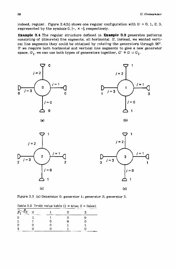
68 U. Grenander

indeed, regular. Figure 3.4(b) shows one regular configuration with G =0, 1, 2. 3,represented by the symbols O. 1-. x -I. respectively.

Example 3.4 The regular structure defined in Example 3.3 generates patternsconsisting of (discrete) line segments. all horizontal. If. instead. we wanted verti­cal line segments they could be obtained by rotating the generators through 90 0

•

If we require both horizontal and vertical line segments to give a new generatorspace. G 1• we can use both types of generators together. G' = G U G1 .

(a)

(e)

(b)

(d)

Figure 3.3 (a) Generator 0; generator 1; generator 2; generator 3.

Table 3.2 Truth value table (1 =true; 0 =false).

~ 0 1 2 3

o 1 1001 1 0 0 02 0 0 1 13 0 0 1 0

Pi.ctU1!8S CIS comptez systems 69

y=L-1 x=L-1,y=L-1•••••

• • •

• • • • • • •• • •

• • • • • • •y=o

x=O x=L-1(a)

x=L-1,y=L-1

x=L-1

1<

X

-) -J -,y=O

x=O

y=L-1

(b)

Figure 3.4 (a) Image produced by (b) configuration with G = 10, 1. 2, 31 = 10 1- x -II.

To make this general we introduce the concept of the bond structure group.Consider a generator spae GO with all its generators of arity NJ (sometimesdenoted c.» and with the bonds enumerated by bond coordinates j = 0, 1, 2, ... ,NJ - 1. The set J of NJ bonds is now subjected to permutations and we choose theset of permutations so that it forms a group (ESC, the bond structure group), butwith no other general restriction.

For example. if NJ =·4 and we allow all rotations, then we can represent thebond structure group as

o 1 2 31 2 3 0

BS'G = 2 3 0 13 0 1 2

where each row is a (cyclic) permutation of J = (0. 1, 2, 3).We now extend the original generator space GO to the extended generator

space GE produced as the set of all generators that can be obtained from GO asthe result of an arbitrary permutation. Returning to Example 3.4, we see that GEconsists of 16 elements (with duplication) and, in general

70

IGE I = IGO I X 1mG I .

U. Grenander

Starting from a generator space G and a bond relation p we have formed theconfiguration space C(R) of all regular configurations over a connecting graph a;R = < p, a >. In this chapter we concentrate on the case where a is fixed inadvance, but in other situations it is necessary to let it be variable, taking valuesin some set ~, the connection type, of possible connectors. We speak of theregularity R as comprising the local regularity, p, and the global regularity, a(or ~).

It was mentioned earlier that the configuration is an abstraction used to syn­thesize the images. An image is what an ideal observer can see, and we haveidentified some configurations in terms of an identification rule R. An image is anequivalence class

I = !c Ic E: C(R), cR col c C(R) (3.2)

of all the configurations that are R-equivalent to a fixed prototype co' The set ofall such images forms the image algebra J. It is an algebra in the sense thatgiven two images, Ii and 12 , we may be able to combine them into a new one,13 =0'0 (11.IiJ. where 0'0 is some new connector. Note, however, that this is onlypossible if R is not violated for the new 13 , Therefore, the algebraic operation isnot always defined (similar to not being allowed to divide by zero for realnumbers). In Example 3.1, if we start from the two images Ii and 12 in Figure 3.5and let the algebraic operation be the combination of I l' moved to the right, with12 , it is clear that local regularity holds for 0'0(11,12), Indeed, the right bond value

5

0 5 10

5

/'0-..0 5 10

5

V0 5 10

Figure 3.5 Images used to illustrate Example 3.1.

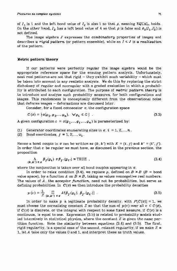
Pictures as compte:r systems 71

of /1 is 1 and the left bond value of /z is also 1 so that p. meaning EQUAL. holds.On the other hand. /2 has a left bond value of 4 so that p is false and ao(/1'/2) isnot defined.

The image algebra J expresses the combinatory properties of images anddescribes a rigid pattern (or pattern ensemble). while an / E: J is a realizationof the pattern.

Metric pattern theory

If our patterns were perfectly regular the image algebra would be theappropriate reference space for the ensuing pattern analysis. Unfortunately.most real patterns are not that rigid - they exhibit much variability - which mustbe taken into account in any realistic analysis. We do this by replacing the strictdichotomy of regular and nonregular with a graded evaluation in which a probabil­ity is attributed to each configuration. The purpose of metric pattern theory isto introduce and analyze such probability measures. for both configurations andimages. This randomness is conceptually different from the observational noisethat deforms images - deformations are discussed later.

Consider. for a fixed connecator a. the configuration space

C(a) = !a(gl' gz... ·, gn)' '\fgi E: G J .

A given configuration c = a(g 1..... gi ..... gn) is parameterized by:

(1) Generator coordinates enumerating sites in a, i = 1. 2, .... n.(2) Bond coordinates, j = 1. 2, ... , c.>i'

(3.3)

Hence a bond couple in a can be written as (k. k ') with K = (i, j) and k' = (i', j ').In order that c be regular we must have, as discussed in the previous section. theproposition

(3.4)

(3.5)

where the conjunction is taken over all bond couples appearing in a.In order to relax condition (3.4). we replace p. defined on B x B (B = bond

value space), by a function A on B x B, taking as values nonnegative real numbers.The values of A, the acceptor junction, need not be probabilities. but serve asdefining probabilities. In C(a) we then introduce the probability densities

- 1 IIp (c) - Z (1e.1e') EO' A [{3j (gi)' (3j'(gd] .

In order to make p a legitimate probability density, with P[C(a)] = 1, wemust choose the normalizing constant Z so that the sum of p (c) over all c E: C (a).if C(a) is discrete, or the integral with respect to some fixed measure. if C(a) is acontinuum, is equal to one. Expression (3.5) is related to probability models stud­ied intensively in statistical physics. where the constant Z is given the name par­tition function. Note the similarity between equations (3.4) and (3.5). The first,rigid regularity, is a special case of the second, relaxed regularity. if we make Z =1, let A take only the values 0 and 1, and interpret these as truth values.

72 U. Grenander

(3.6)

(3.7)

It is convenient to write equation (3.5) in a slightly different form, mathemat­ically equivalent, but easier to manipulate during the design of inferencemachines, discussed later; namely,

PT (c) = 1.. IT Q(g1.) n AJ-IT [~j (g1.)' ~j,(g1. ,)] .Z1.=l (1e,1e')Ea

Here Q is a density in the generator space G, A o is a fixed acceptor function, andT a positive parameter called the temperature of the pattern, in analogy withstatistical physics. If we write

A o(~, ~') = exp ao(~, ~') ,

where a o should be thought of as the affinities between bond values, we obtain

1 N {1 }p(c) =-z r:! Q(g1.)exp -T ~ aO[~j(g1.)' ~j' (gd]1. -1 (1e,1e')Ea

The role of Q is to give different emphasis to different generators. It is notthe same as the marginal distribution of all g s in the random configuration c, butis useful for easy manipulation of the probability measure when we want toincrease or decrease the occurrence of a particular generator.

What happens when T .... O? Well, if ao(~', ~") is positive, then (lIT)­a o(~', ~") becomes very large, and if it is negative, then (1/ T) ao (~', ~") becomesvery small. Hence a small T accentuates any difference in affinities between bondvalues. Certain configurations, where the bond values fit well, have large proba­bilities, and so all others are highly unlikely. Therefore, cold patterns will. withhigh probability. become regular in the sense of the bond relation

~. p r <~ aO (~', ~") = max ao (~1' ~2) .flt, 112

The opposite case, T .... co , renders the exponents in equation (3.7) close tozero, which means that the generators in c behave, almost, as an LLd. sample fromG with the marginal distribution equal to (actually proportional to) Q. Hence hotpatterns are purely random and very chaotic. It is only in this special case thatQ represents the marginal distribution.

The probability density p in equation (3.7) on C induces a probability mea­sure on J equal to the set of all, R-equivalence classes of C, so that an image I, ora set of R-equivalent configurations I E: J, I E: C, has the probability

P(/) = ~ p (c) .eEl

For any fixed T, P in equation (3.7) represents a flexible pattern. It is arelaxed form of the regularity described by an image algebra.

Example 3.5 First a simple example: suppose that G = !O, 1! with ~ j (g) == g, andthat we use the trivial identification rule R = (0, 1), so that configuration heremeans the same thing as image, and suppose the acceptor matrix is

(1.1]A = .1 1 = (aleL:k,l =0,1) .

A typical image is given in Figure 3.6, and shows little geometric activity.

P1.ctures as compLez systems 73

i -.-:.-:.-:.7.-::-:::::.7-- -;::-:.7.7.7.--- - - - - --- - - --II ••••••••••••••••••• ••••••••••• II ••••••••••••••••••• ••••••••• •••••••••• II····················· .•.... *~. *.*.****·*··1I······················· *··.**···***1I························ .•. · ·····1I························ .•••.•••..•. ,I························ .•. ·· ••• ····1,........................................ ** •••••••• ,,........ . ....•.•....•.....••...'..... .**·**····1,•••• ** •••••••••••••••••••••••••••• • •••••• ,1···*** ...•.....•................. ·······1I······ .....•••••..•...•.•.....•• *·*·*1I···· ...•....................... ···1I···· ...... .•..•....•....•...•...•.... .....•••......•.......•••••...............•..•.............••........•....••......•...•.•.........•....•.•.. ...

*•• • ••••-••• I.......................····1........................ ···1. ····1.......................······1. ·.···1••••••••••.•••••••••••••••'••••• I..........................····1........................·.···1............................. ,..................- ·,···1. ····1.................... ··1

•• ••••••••••••••• ••••••••••••••••••••

**

1***I·······I··········· .•..•..I·····················, ••••••••••••••• *••• * ••••1*···*·················*·1*····*··**·····**···*···1··*·***·········*··**·**1····*······*·***·**·**·*1·**········*·***·*·***··,*•••••••••*.**.***••*.**••••1*·········***·***·*****·*···,*••••••.•**••*•••*••*** •••••••••••••••**.**•• **.** ••*•••

•••••••*•• *••***••••••••••••••••••••••••••••

**•••••••••••••••••*••••••••••••*.*•••••••••••••*.*•••**••••••••*.**••••••••••••*•••••*•••••••••• *•• *•••••** •••••••*•••••• *•••••• * ••••••••••••••...................................•.....................•.....................••..••...•.•..........•..... ..•..•....•...............•........•.•................•.•...•• , •.••..•..•..........•..•.........•..... •........ ,...•...........,.. . , ..••..•••••....•... , ,., .•....•.....•...... . ,., .. ,

Figure 3.6 Image t.ypical of Ell:llmple 3.5.

If we increase the size of the entry a. 01 = a. 10 = .1, the picture becomes morechaotic; if we lower it the picture contains larger clumps of zeros or ones. Thiscan, of course, also be achieved by replacing A with

AT = fa.it T; k, l = 0, 1l

74 U. Gre'll.a'll.cter

Example 3.6. If we use the generators in Example 3.6 with the acceptor matrix

1.01 1.01 01]A = 1.01 .01 .01

.01 .01 1.00

and if we identify 0 with a blank and 1, 2, or 3 with a star we obtain, in one partic-ular case, the configuration shown in Figure 3.7. Note that horizontal segmentssuch as 12223 are surrounded by zeros. This configuration corresponds to theimage in Figure 3.8.

0 0 0 0 0 0 0 0 0 0 0 0 0 0 1 2 3 0 0 1 3 0 0 0 0 0 1 3 0 1 3 0

3 0 0 1 2 2 3 0 0 1 3 0 0 0 0 0 0 0 0 0 0 0 0 0 0 0 0 0 0 0 0 1

0 1 3 0 0 0 0 1 3 0 0 1 3 0 1 2 3 0 0 0 1 2 3 0 0 0 0 1 3 0 0 0

0 0 0 0 0 0 0 0 0 0 0 0 0 0 0 0 0 0 0 0 0 0 0 1 2 3 0 0 0 0 1 3

0 0 0 0 0 0 0 1 3 0 1 2 2 2 3 0 1 2 3 0 0 0 0 0 0 0 0 1 2 0 0 0

0 0 0 0 1 3 0 0 0 0 0 0 0 0 0 0 0 0 0 0 0 0 0 1 3 0 0 0 0 0 0 0

1 3 0 0 0 0 0 0 0 0 0 0 1 3 0 0 0 0 0 0 0 1 3 0 0 1 2 3 0 0 0 0

0 0 1 3 0 1 2 2 3 0 0 0 0 0 0 0 1 3 0 1 3 0 0 0 0 0 0 0 0 0 0 0

0 0 0 0 0 0 0 0 0 0 0 0 1 2 3 0 0 0 0 0 0 0 0 0 0 1 3 0 0 0 1 3

0 0 0 1 2 3 0 0 0 0 1 3 0 0 0 0 0 0 0 0 0 0 0 0 0 0 0 0 0 0 0 0

0 0 0 0 0 0 0 0 0 0 0 0 0 1 2 2 3 0 1 2 2 2 2 3 0 0 0 0 1 2 3 0

0 0 0 1 2 2 2 2 2 3 0 1 3 0 0 0 0 0 0 0 0 0 0 0 0 1 2 3 0 0 0 0

1 3 0 0 0 0 0 0 0 0 3 0 0 0 1 3 0 1 3 0 0 0 0 0 0 0 0 0 0 1 3 0

0 0 1 3 0 0 0 0 0 0 0 1 2 3 0 0 0 0 0 0 0 0 0 1 2 2 2 2 3 0 0 0

2 2 3 0 0 0 1 2 3 0 0 0 0 0 0 0 0 0 0 0 1 2 3 0 0 0 0 0 0 0 1 2

0 0 0 0 0 0 0 0 0 0 0 0 0 0 0 0 0 0 0 0 0 0 0 0 0 0 0 0 0 0 0 0

0 0 0 0 0 0 0 0 1 2 2 3 0 0 1 3 0 0 1 2 3 0 0 0 0 0 0 0 1 3 0 0

0 0 0 1 3 0 1 3 0 0 0 0 0 0 0 0 0 0 0 0 0 0 0 0 0 1 3 0 0 0 0 0

0 0 0 0 0 0 0 0 1 2 2 2 2 2 3 0 0 1 3 0 0 0 1 2 3 0 0 0 1 2 3 0

0 1 2 3 0 0 0 0 0 0 0 0 0 0 0 0 0 0 0 0 0 0 0 0 0 0 0 0 0 0 0 0

0 0 0 0 0 0 0 0 1 3 0 0 1 2 2 2 2 3 0 0 0 0 1 3 0 0 0 0 0 0 0 0

0 0 0 1 2 2 2 3 0 0 0 0 0 0 0 0 0 0 0 0 0 0 0 0 1 2 3 0 0 0 1 3

0 0 0 0 0 0 0 0 0 0 0 0 0 0 0 0 0 0 0 1 3 0 0 0 0 0 0 1 3 0 0 0

3 0 0 0 0 0 0 0 0 0 0 1 3 0 0 0 0 0 0 0 0 1 3 0 0 0 0 0 0 0 0 1

0 0 1 3 0 0 0 0 0 0 0 0 0 0 0 0 0 0 0 0 0 0 0 0 0 0 1 2 3 0- 0 0

1 3 0 0 1 3 0 1 2 3 0 0 0 1 3 0 0 0 0 1 2 3 0 0 0 0 0 0 0 0 0 0

0 0 0 0 0 0 0 0 0 0 0 0 1 0 0 0 1 3 0 0 0 0 0 0 0 0 0 1 3 0 1 3

0 0 0 1 2 3 0 0 0 0 2 3 0 1 2 3 0 0 0 0 1 2 2 3 0 0 0 0 0 0 0 0

0 0 0 0 0 0 1 2 3 0 0 0 0 0 0 0 0 0 0 0 0 0 0 0 0 0 0 0 0 0 0 0

2 2 2 3 0 0 0 0 0 0 1 3 0 1 2 3 0 0 0 0 0 1 2 2 2 3 0 0 0 0 1 2

0 0 0 0 0 0 0 1 3 0 0 0 0 0 0 0 0 0 0 0 0 0 0 0 0 0 1 3 0 a 0 0

0 0 0 1 2 3 0 0 0 0 0 1 2 0 0 0 0 1 2 0 0 0 1 2 2 3 0 0 0 a 0 0

Figure 3.7 Configuration typical of Example 3.6.

If we change the temperature from T =1 to T =10 for the situation given byFigures 3.7 and 3.8 we obtain the configuration in Figure 3.9. It is obvious how farwe are here from the local regularity p of Example 3.1. Ones occur together, theright and left endpoints appear at the wrong end, so chaos reigns. Thecorresponding image, Figure 3.10, is very hot; lines crowd each other (note, espe-cially, the top) and little stnlcture is visible. This case is used repeatedly in thefollowing as an illustrative example. The pattern itself is of no interest, but serves

Pictures eu compLez systems 75

*** ** ** *** **** ** *

** ** ** *** *** ***** **

** ***** *** **** **

** ** ** ***** **** ** **

*** ** ***** **

**** ****** ********** ** ***

** * ** ** **** *** ******

*** *** *** **

**** ** *** **** ** **

******* ** *** ******

** ****** ******* *** **

** *** ** ** *

** ***** ** *** ** ***

* ** ** *ii

*** ** *** *******

**** ** *** ***** **** **

*** ** ** ****

Figure 3.8 Image produced by the configuration of Figure 3.7.

a didactic purpose. We have not said anything about the method of pattern syn­thesis used to give these pictures. It is far from easy and is discussed later.

Deformation of images

Equation (3.7) defines a probability measure P, which serves as a prior inthe Bayesian approach. In addition to the randomness described by this prior weneed another source of randomness to deform the image, called D, a deformationmechanism:

D : J .... JD = a set of possible deformed images.

In linear inference the most common assumption is that D acts additively: theonly effect is to add random noise n to I, ]D = I + n. This is called additivenoise deformation, and is a special case of contrast deformations. Anothercontrast deformation is the symmetric binary noisy channel which works as

76 U. GrenGnder

0 3 0 0 2 3 0 1 2 2 1 1 2 3 2 1 1 0 0 1 0 0 1 1 0 1 2 2 1 0 2 31 3 3 0 0 0 1 3 1 1 2 2 2 1 2 1 2 2 3 2 0 3 2 3 1 2 3 1 0 1 2 03 2 1 2 0 1 0 0 2 2 2 2 0 2 1 3 0 2 1 1 3 3 3 3 0 0 2 0 2 0 1 23 0 2 0 1 0 0 1 3 0 1 2 1 0 3 1 3 0 3 1 2 3 0 1 2 3 3 1 0 0 1 10 0 2 2 1 2 3 0 0 0 0 0 0 1 2 2 0 1 0 0 3 2 3 3 3 1 3 0 1 3 0 01 2 0 0 0 1 3 2 2 1 3 3 0 2 0 0 0 0 0 0 3 0 0 0 1 0 2 0 0 2 2 30 2 2 3 0 0 0 2 1 3 0 1 2 0 1 3 2 1 2 1 3 3 2 1 2 2 0 0 2 3 1 30 1 0 0 0 2 3 3 0 0 2 3 1 0 0 3 3 0 1 3 1 0 1 1 1 2 2 0 0 1 2 01 0 0 0 1 1 3 2 0 3 0 0 1 3 0 2 0 0 1 2 0 0 2 3 0 0 0 3 2 0 1 22 1 0 0 0 1 0 0 1 2 3 0 1 1 0 1 3 0 3 2 2 2 1 0 1 0 0 1 3 2 1 22 3 0 0 2 2 2 3 2 0 0 1 1 1 2 1 1 1 0 0 0 3 1 2 2 2 0 1 1 1 0 00 2 2 3 0 0 1 3 0 3 1 3 1 0 2 1 0 1 3 1 2 0 0 0 0 0 1 2 0 2 0 30 0 3 1 0 1 1 0 1 0 0 0 1 0 2 0 0 1 0 1 2 3 1 0 1 3 0 1 0 0 0 01 2 2 2 0 1 3 2 1 2 2 0 0 0 0 3 0 1 0 1 2 3 2 0 1 0 3 1 1 0 0 00 0 0 1 0 0 1 3 0 0 2 3 2 0 2 2 2 1 2 0 1 3 1 3 0 3 1 2 2 1 3 02 2 1 2 3 0 0 0 0 1 0 3 3 0 0 1 0 0 0 1 3 3 2 0 1 0 0 3 0 0 1 33 0 3 3 3 1 1 3 0 0 1 3 1 0 0 3 1 0 0 2 2 1 3 0 0 1 2 0 3 0 0 01 0 2 3 1 0 0 2 1 1 3 0 3 0 3 0 2 2 1 3 3 0 0 1 1 3 0 1 0 0 0 31 3 0 0 0 0 3 2 0 3 1 3 3 3 0 0 1 0 2 0 2 1 1 0 0 0 1 3 1 3 2 20 0 2 1 3 2 3 0 0 0 0 0 0 1 2 2 3 2 2 3 1 2 0 1 2 1 0 0 0 0 3 31 3 2 3 0 1 3 3 0 0 0 0 3 3 1 0 0 0 1 0 3 2 3 2 3 3 0 3 0 0 3 01 0 1 0 3 0 0 0 1 1 2 3 3 1 3 0 0 3 1 2 2 0 0 3 2 2 2 1 0 1 0 23 3 2 2 2 1 3 1 3 0 2 2 3 1 1 2 3 1 2 1 2 2 3 3 0 0 1 0 2 2 2 00 0 0 0 1 3 0 0 1 3 2 0 2 0 0 1 0 3 3 0 0 0 0 3 0 3 1 2 0 0 0 01 1 2 3 2 3 0 0 1 0 0 0 0 0 0 0 0 0 1 2 0 1 0 1 2 3 0 2 1 0 2 02 3 0 0 0 0 0 2 3 1 2 1 2 3 1 1 2 3 0 0 3 0 1 3 2 3 0 0 2 0 2 03 0 2 2 0 0 1 3 1 1 2 0 0 2 1 0 2 3 3 3 0 0 0 0 0 0 2 3 2 0 1 23 0 1 0 3 2 0 3 0 0 3 2 1 0 3 2 3 2 3 1 2 3 0 1 1 2 2 2 1 3 2 22 0 2 0 0 0 1 1 2 1 0 3 0 3 0 1 1 2 0 0 3 2 0 1 1 3 3 0 0 0 0 00 1 2 1 3 1 2 2 3 2 1 0 2 0 3 1 0 2 2 1 1 2 3 0 0 0 1 0 2 2 3 03 0 0 0 0 0 2 0 0 3 0 1 3 3 1 3 1 0 0 0 2 3 1 1 2 0 1 2 0 0 3 11 3 2 2 3 3 0 2 1 0 2 0 0 3 1 0 2 3 2 1 2 1 3 0 0 1 1 3 0 3 0 1

Figure 3.9 Case of Figure 3.7, but with T = 10.

* ** ********** * ** **** ***** ************** ******* ****** * **** *** ******* * * *** * * ** *** *** •• ** ***** **

***** *** * ******* **** ****.*. * * * * ***

*** *** ** ************ ***** *** *** ** *** ***** **

* **** * ** * ** ** ** **** * *** ** ** ***** * ******* ***** ******* ***** ***

*** ** **** ** **** ** * *** ** * * * * **** ** *

.*** ****** * * **** * **** ** *** ***** **** ******

***** * ** * **** * * *** ****** *** ** **** ** ** *** .*** * * ***** *** * *** ** ***** * * *** .*****

***** ********* **'" ****** *** *** * ****** * ** * * * ••• *** **** ***** * ****.***** ************** * ***

** *** * * ** * ********* * ** * *** ** *** *********** * **** * ** ** ***** ** **** *** *** ... ** * *** ******** ********** * **** * * *** ** ****

********** * ** ****** * **** * * ****** ***** ** ******** ** * ** ******* *** * *

Figure 3.10 Image produced by the configuration of Figure 3.9.

Ptctures as compLex systems 77

(3.8)

follows. Let the pure image i = I (x , y) be a black and white picture so thatI(x, y) takes only two values, say 0 and 1. Then we define, for a fixed I, that forv = 0 or 1,

D {1 - e if I(x, y) = vP[I (x,y) =vII] = e if I(x,y) =l-v

Note that the probabilities of the error 1 ... 0 or the error 0 ... 1 are the same (Le.symmetric).

Sometimes we have nonrandom deformations. An important case is blurring,which acts on contrast patterns where the contrast values are in some linearspace, say, the real line, I(x, y) E R. Then the deformed image is the convolution

ID(x, y) = l: w t.,.,I(x -~, y - 77) . (3.9)t. .,.,

Usually the range of summation is small compared to L. An example is

I 1 2 if 0 sl~I,I771 shw t.,., = (2h + 1) .

o else

a rectangular window, but it is more common to have less sharp windows: w t.,.,goes to zero smoothly as I~I and 1771 become large. Another nonrandom D is themask deformation. If I(x, y) is defined for 0 s ~,77 < L then

I D = !I(x,Y)I(x,y) EMl '

where M is a sebset of 'Zl Some of the observations have become hidden from theobserver.

Before we discuss inference machines, let us summarize how we introduceregular structures:

Step 1

step 2

step 3

step 4

step 5

step 6

Choose a connector, a, which is a graph with sites where the generatorsmay reside. So far we have examined only very simple. regular connec­tors, but we later show how several levels within a can be useful.Choose a generator space, G, with special attention given to the actualmeaning of the bond values - the signals exchanged by generators. Thisis the crucial step, demanding inventiveness and intuition.Introduce the rigid regularity by a bond relation. p. corresponding tothe type of ideal patterns that we began with.Describe what the ideal observer is allowed to see by an identificationrule R. This is usually easy.Relax the regularity by replacing p with an acceptor function, as inequation (3.7).Study the deformations caused by imperfections in instrumentation andtransmission.

We are now ready to study the process of pattern inference.

78

Introducing Pattern Inference Machines

U. Gren~ncter

The starting point when constructing inference machines is the question:How can we simulate probability measures of the form (3.7)? We want a systematicmethod for generating a random sample of LLd. observations from C or J obeyingequation (3.5). In other words, we are attempting pattern synthesis.

There are two reasons why pattern synthesis plays a central role in ourapproach. The first is obvious - we want to synthesize images to judge whetherthe pattern model actually gives patterns of the type we want. The second, andthis is the more important, is that all our analyses and inferences will be based onpattern synthesis. This claim, that analysis can be done by synthesis, may appearparadoxical, but we shall show that it is true.

The Markov property

The probability measure P can be said to be regularity controlled, since itis driven by the acceptor A, which mimics the bond relation p that expresses therigid regularity. P is a very large family of measures, too large, and must be made

..... '" ,\ C\III

I

Figure 3.11 Configuration withc = a (g o.g l.g z.g 3.g 4.g fj.g 6,g 7,g 8·g g,g 10·g 11)c' = a' (gB,g9)c" = a"(go,gl. g Z. g 3,g4,gfj.g6. g 7,g10. g 11)c'" = a"'(g4. g fj.g6,g7.glO,g11)

I:'I

P1.ctures ~s compte% systems 79

specific by choosing a particular A. or a small family of As. But before this can bedone, we must first understand one fundamental property that all these Ps have incommon. For simplicity we assume that:

(1) The generator space G is finite, IG I = r < ""'.(2) The acceptor function (acceptor matrix) A takes only positive values.

Both of these conditions can be relaxed.Consider the configuration diagram in Figure 3.11. In the configuration c we

select a subconfiguration. c', and consider c as the connection of c' with theremaining subconfiguration c ".

c =ao(c',c").

Let us calculate the conditional probability using the general equation (3.5).

P( 'Ie") = P(c' and c ") =..£.JEJ... .c P(c") P(c")

The constant Z cancels since it appears in both numerator and denominator andwe obtain

with the notation k = (i. n, k' = (i ',n for the generator and bond coordinates,and where the summation extends over all generators in c'. However. a lot of fac­tors occur in both the numerator and the denominator, and so can be canceled.Indeed, all generators that are not connected with the subconfiguration c' canceland we, therefore, obtain (with obviously abbreviated notation),

[ (Ie, p) E a A]P (c ' Ic ") = ~-----------''­

I: A(Ie, Ie') Ea'"

where the new subconfiguration c = a" (g1. ,g1. .... ) (see Figure 3.11) consists of1 2

the outer boundary of c ": the set of generators that are not contained in c' butborder it. In summary, we have shown that

p(c'lc") =p(c'lc''') ;

that is, the probability depends only upon the outer boundary c'''. not on all theouter generators in c ".

This is a Markov property, generalizing the idea of a Markov chain or Markovprocess. We are, therefore, in a general sense dealing with Markov processes(sometimes called Markov random fields) and our task is to invent methods ofinference in Markov processes (partially observable).

eo

Simulation lor pattern synthesis

U. Grenanaer

To provide a pattern synthesis for a given relaxed pattern P we need analgorithm that generates a random configuration from the pattern P. No directmethod is known for doing this - we are forced to apply an indirect one. which isbased on the Markov property discussed in the previous section. Select a site i 1and consider the generator g1. there. Conditioned by the rest of the configura-

I

tion it has some probability distribution Pi' Let us update c by replacing g.1·1

with a random generator g; which has been generated from Pi . We discuss later·1 I

(p 81) exactly how to do this and only remark here that Pi I depends only upon the

immediate neighbors of gil'

Now we select another site. i z. and replace g1. e by some gi. e simulated under

the probability law Pi . Proceeding in this way we obtain a sequence of configura-2

tions. c 1 ,c Z.c 3 ,.... c t ..... which can be thought of as an ordinary Markov chain intime. The state space is C. probably of enormous cardinality. but finite underassumption (1) of the previous section.

We have not specified how the sequence i 1 • i z.... should be chosen and prefernot to do so completely yet. Suffice it to say that each site i must be visited infin­itely often during the sequence for the following reasoning to hold true. It is notdifficult for anyone familiar with Markov chains to see that the probability distri­butions of c t converge to a unique equilibrium distribution. But the probabilitydistribution P in equation (3.5) is certainly in equilibrium: just recall how weupdate Ct. Hence the limiting distribution of Ct. t .... "". is the P we want to simu­late.

It should be pointed out that while the probability distributions will con­verge. the configurations c t themselves will not. They will continue to vary dur­ing the updating and will not settle down to a particular one. Let us extend this:it is not necessary to update a single site at a time. The reasoning above remainsvalid if. at time t. we update several sites at once. so long as no two of these sitesare neighbors. At time t =1 we can update all sites in S1' at t =2 all sites in Sz.and so on. where the St. the sweep areas, are subsets of ~1. 2 ... ,. n l.

And this is where recent advances in computer technology appear as ifpreordained. If we have access to a parallel computer with many processors (pro­cessing elements or PEs) working at the same time. we can apply each PE to updat­ing each generator in a sweep area. Then we change from sweep area to sweeparea. If the sweep areas are large we can speed up the pattern synthesisdrastically.

Which sweep areas to use depends on the topology induced by the connectora. For a square lattice with NJ = 4 neighbors two sweep areas are enough. oneconsisting of the rings and the other of the crosses in Figure 3.12(a). If NJ =8 weneed four sweep areas. as in Figure 3.12(b) and indicated by the four symbols usedtherein. For a general a the number of sweep areas required equals the chromaticnumber of the graph; that is. the number of colors needed to color the graph sothat neighbors have different colors.

Sometimes we violate the condition that no two sites in a sweep area beneighbors. which improves convergence but at the cost of increased computertime for the individual updating. since the above rules do not apply and have to bereplaced by more complicated ones.

Ii

P1.ctures as compLex systems

=R)----l

I I~

(a) (b)

81

Figure 3.12 Sweep areas for connectors with (a) NJ =4 and (b) NJ =8.

The choice of sweep areas, the sweep strategy, is not well understood atpresent. Moreover, only scanty knowledge is available as to the number of itera­tions (the relaxation time) needed before the probability distributions convergesufficiently to the equilibrium distribution. Many computer experiments have beenperformed to study this and the conclusion is that warm images are easy to syn­thesize; the convergence is fast. Cold images take longer to synthesize.

These empirical results have recently been supplemented by an analyticalone. A theorem, which we quote without proof and without complete specification,states that the relaxation time

t :> a 7/ Trelax - e

where a and "'I are positive constants. It follows that as the temperature T dropsto zero, the relaxation time increases exponentially. This explains our empiricalfindings and should serve as a warning when highly rigid patterns are encoun­tered. The scheme described here is called stochastic relaxation.

stochastic relaxation for pattern inJ'erence

To see how synthesis via stochastic relaxation is directly related to syn­thesis, examine Figure 3.13. It shows a six-level configuration, viewed from theside, so that, for example, level three actually has 16 generators but appears tohave only four. The connector is fairly simple; if it were not for the horizontalconnections in the level h = 2 it would be simply a tree. The two lowest levelshave a special significance. Consider two configurations c' and c" with the con­nector of Figure 3.13 and identify them, such that c' R c ", if and only if they coin­cide at h = 1, c:1 =c 1'. This identification rule implies that the equivalenceclass of R-equivalent configurations is determined by the first level, so we can sim­ply say that the second level c2 is the image.

In the computer experiment that produced Figure 3.13, the identificationrule R was induced by an equivalence relation R on the generator space (see alsoExample 3.6). Hence, the acceptor function that appears in a bond couplebetween g 2 at h = 1 and g 1 at h = 2 can be written

R R) _ {1 if g2 belongs to the equivalence class of glA (/"1' 1"2 -

a else

82

h=5

h=4

h=3

h=2

h = 1

h=O

U. Grenander

Figure 3.13 Side view of a six-level configuration.

Here the (Js equal the gs; they are full information signals.The lowest level. h = O. plays the role of the deformed image, [D, which is

actually observed by the available instrumentation. In this example, a generatorg2 at h =1 and a generator gl at h =0 were related by the acceptor function

A({Jl,{J2) ={1 - eif gl =g2e else

In other words, D is a symmetric, binary noisy channel with error probability e.To summarize: level 0 is the deformed and observed image [D, level 1 is the

pure image [ that we want to see, and the upper levels constitute the analysis orgeneration of [. Whether we want it for its own sake or not. the analysis must beincluded in the inference procedure.

The pattern inference procedure can now be run. The generators at h = 0should be fixed as the values observed in [D; the remaining levels can be givenarbitrary values (but one can do better than that if speed is of importance). Wethen update all the sites (except for h = 0) in the total configuration using theupdating procedure described above. with some sweep strategy. After a number ofsweeps the probability distributions settle close to equilibrium. In this case. sincewe fix [D. the marginal probability measure for [, h =1, tends to equilibrate withP according to equation (3.9)

ptUI[D) .... p([I[D). as t .... DO • (3.9)

This can be immediately used for pattern inference of the Bayesian type.

Pictures as compLex systems 83

(3.10)

We started with a prior for I and simulated the posterior on the right-handside of equation (3.9). But the Markov process in time is (asymptotically) station­ary and ergodic so that we can estimate I by a procedure of averaging type.The exact form of the procedure depends upon what optimality criterion we use. Ifthe Is are binary and we adopt Hamming distance as the optimality criterion.

so that we want to find a restored image 1*. with E[d (I. l*)] a minimum, we shouldchoose 1* using rule (3.10)

l*(x,y) ={liffn(X,y)~t1/2oelse '

where we have run the inference process for the iterations t =1,2, ...• t l' andf n (x, y) is the number of iterations for which we have observed a 1 at site (x, y)in h =1. On the other hand, if G = R and we want to minimize the expected L zdistance, we should choose the restoration procedure

1 t 1

l*(x,y) =-t- 2: ci(x,y)1 t =1

Space does not allow us to discuss the refinements of such procedures. Itshould be mentioned, though, that substantial increases in the process speed cansometimes be obtained by variable temperature schemes, large sweep areas, andcareful initialization.

It is important to realize that these procedures do not simply guarantee con­vergence. They are the best possible ones under the given conditions: the pat­tern inference process exploits the available information optimality. Wehave thus seen that, just as the process can synthesize patterns, it can alsoanalyze (infer) patterns. It realizes the maxim

PATTERN ANALYSIS =PATTERN SYNTHESIS.

Let us now look at other types of pattern analysis in addition to inference.Suppose that the image has been masked from view (see the section on deformationof images, p 75): only certain sites, (x, y) E: MC can be observed (with or withoutpattern deformation). We then initialize the process by fixing the values at thesesites to be the observed values, letting the rest be arbitrary. The process is runfor a number of sweeps, level 1 observed, and the above procedure used, whichresults in optimal extrapolation from MC to all sites.

Suppose that D blurs the image by convolution, as discussed earlier, withwidth 3. Then the three lowest levels of Figure 3.13 appear as in Figure 3.14 (theupper levels are not shown as they are exactly as in Figure 3.13). Remember thatthis is a side view; the object is really a set of planes. In Figure 3.14 the twoupper levels are connected by bonds that express a deterministic relation as inequation (3.8). The two lower levels are connected by bonds that express stochas­tic relations, for example, a binary noisy channel.

Once it is realized that, because of the locality of blurring operations, wecontinue to obtain joint probabilities as before, it is clear that we can run thepattern inference process again with the lowest level, h = 0, fixed in order torestore the pure image at h = 2. In this way the picture is simultaneously

84

h=2

h=1

h=O

U. Grenander

Figure 3.14 Lowest three levels of Figure 3.13 when D blurs the image by convolutionwith width 3.

h=3

h=2

h=1

h=O

Figure 3.15 Level h =0 is the observed image and the generators at h =3 are binary.

unbLurred and cleaned of noise, as far as is possibLe given the informationcontained in I D . Consider Figure 3.15 in which, again, h = a is the observedimage. Let the generators allowed at h =3 be binary; that is, the only values areon and off.

We observe I D , fix h =a to the values observed, run the inference process anumber, t l' of sweeps, and record how many times each of the generators at thesite i were on the maximum level, h =3. If such a number is greater than t 1/2 wesay that we have recognized object i in the picture, otherwise not. This meansthat the inference process achieves optimaL pattern recognition under thegiven conditions.

Examples of inference processes

We illustrate the general procedure described above with two simple exam­ples. The programs are not described herein.

First, we discuss the pattern synthesis that underlies the picture shown inthe section on metric pattern theory. In Example 3.5 we used a 2-D toroidal

Pictures as complex systems 85

lattice of size L x L, and updated according to the scheme of rings and crosses, asshown in Figure 3.2(a); we initialized this at random. After implementing the res­toration by computer programs we ran the process to obtain optimal recognition.An example is shown in Figure 3.16, where I is the pure image. ID is the deformedimage observed by the viewer, and 1* is the restored image. The results from run­ning this pattern inference process speak for themselves.

(a) (b) (c)

Figure 3.16 (a) Pure image (I), (b) deformed image observed by lhe viewer (/D), and (c)reslored image (1*) for Example 3.5 (I is as in Figure 3.6).

(a)

..... .........

...... ........... .. .

(bl

.. ............. ..... ..

(e)

Figure 3.17 (a) Pure image (I), (b) deformed image (lD), and (c) reslored image (/*) forhorizonlalline segmenls and relaxed regularily.

86 U. Grenancter

In our second example, in which we have horizontal line segments and relaxedregularity, we developed similar computer programs. Figure 3.17(a) shows a syn­thesized pure image, 3.17(b) the deformed image, and 3.17(c) the restored one. Thelatter has recovered much of the lost structure and the error rate has beenapproximately halved.

The patterns used so far as illustrative examples were synthesized from cer­tain given generators and acceptor functions We conclude the chapter by showinga real pattern analyzed by S. Geman, D. Geman, and D. McClure (unpublished). Theimage in Figure 3.18(a) was drastically deformed by additive noise, Figure 3.18(b).The restoration algorithm produced the image shown in Figure 3.18(c).

(a) Ib)

(c)

Figure 3.18 (a) Blurred image (roadside); (b) degraded image due to additive noise; and(c) restored image inciucting the line process (1000 iterations).

The successful application of general pattern theory to picture processing,or to the analysis of other complex systems, requires a thorough examinationof the basic elements: the generators, the connector graph, and the acceptor

Pictures as compLex systems 87

functions. In addition, the corresponding soft- and hard-ware problems must besolved, challenging tasks which have been accepted by a number of researchers.The prospects look promising, but what is absolutely essential is collaborationwith other scientists who have knowlege of particular subjects: biologists, physi­cians, psychologists, linguists, and others.

The reader who wishes to learn more about this pattern theoretic researchshould consult the author's series Lectures in futtern Theory, 3 volumes,Springer Verlag, 1976, 1978, 1981.

CHAPTER 4

A Survey of Replicator Equations

Karl Sigmund

Introduction

What are the units of natural selection? This question has aroused consider­able debate in theoretical biology. Suggestions range from pieces of polynucLeo­tides. genes. or gene complexes to individuals. groups. or species. It could be.however. that different answers are correct in different contexts. depending onthe scale on which selection acts most decisively. This is somewhat analogous tophysics. where the dominant force may be gravitational, electromagnetic, orstrong or weak interparticle attractions, depending on the problem.

It is therefore convenient to consider an abstract unit of natural selection intheoretical investigations. which can be replaced by the appropriate real unit(genes, individuals. or species) in specific circumstances. This abstract unit istermed a replicator in Dawkins' book The Extended Phenotype (Dawkins. 1982).The term describes any entity which (a) can give rise to an unlimited (at Least inprinciple) sequence of copies and (b) occurs in variants whose properties mayinfluence the number of copies.

Biomathematical arguments support the usefulness of this concept. Indeed.the remarkable similarity of dynamical systems describing the action of selectionin the most diverse fields lends weight to the notion of a common mechanismunderlying these different observations. The term replicator dynamics has beenapplied to this mechanism (see Schuster and Sigmund. 1983). In the case of con­tinuous time (generations blending into ea.ch other). the dynamics ca.n bedescribed by an ordinary differential equation x =F(x) of the type

X." =x.,,[f.,,(x)-lfl]. i =l •.... n (4.1)

while for discrete time (separate generations) the dynamics are given by a differ­ence equation x -0 Tx with

(Tx)." =x." [f"'~X)]. i =1, ... ,n (4.2)

A Survey ojRlIpL1.cator Equa.tio7l.s

In both cases. the term c{l is defined by

71.c{l(x) = LXiIi (x)

1.=1

and ensures that the state x of the system remains on the unit simplex

89

(4.3)

71.371. =~x =(x 1 .···.x7l.) ER7I.: LXi = 1. xi ~O for all ij . (4.4)

1.=1

The functions 11. (x) describe the interaction of the different variants of theunderlying replicator and are specified by an appropriate biological model.

In particular, first-order interaction terms. that is linear functions11. (x) =(A x)1. defined by a matrix A = (a1.j)' where

71.(A x)1. = L a1.j x j (4.5)

j=1

lead to dynamics which have been investigated independently in (i) populationgenetics. (ii) population ecology, (iii) the theory of prebiotic evolution of self­replicating polymers. and (iv) sociobiological studies of evolutionarily stable traitsof animal behavior. Within these contexts. the dynamics describe the effects ofselection upon (i) allele frequencies in a gene pooL (ii) relative frequencies ofinteracting species. (iii) concentrations of polynucleotides in a dialysis reactor.and (iv) distributions of behavioral phenotypes in a given species.

After a brief summary of the biological background in the following section.we present a survey of the mathematical aspects of continuous- and discrete-timereplicator equations. There are many interesting results. in particular for thefirst-order case, due to the work of Akin. Hofbauer. Zeeman, and others. On pages93-94 we are concerned with some general properties of replicator equations andon pp 94-95 we discuss the existence and stability of equilibria and present sometheorems on time averages and exclusion properties. Results concerning the per­manence of the biological components of the system are presented on pp 96-98.Gradient systems for replicator equations are then described. followed by anoverview of the classification of low-dimensional phase portraits. Finally, we sum­marize the relationships between game theory and first-order replicator equa­tions.

Biological Motivation

Population genetics

Genes are the quintessential replicators. It is therefore quite appropriatethat the first systematic study of a class of replicator equations occurred in popu­lation genetics: the classic work of Fisher. Haldane. and Wright on the effects ofnatural selection upon the frequencies of alleles at a single locus of a diploid. ran­domly mating population.

Briefly. if A 1 .... ,A7I. denote the possible alleles and x 1 ..... x7I. their frequencieswithin the adult population, then random fusion of gametes yields zygotes of

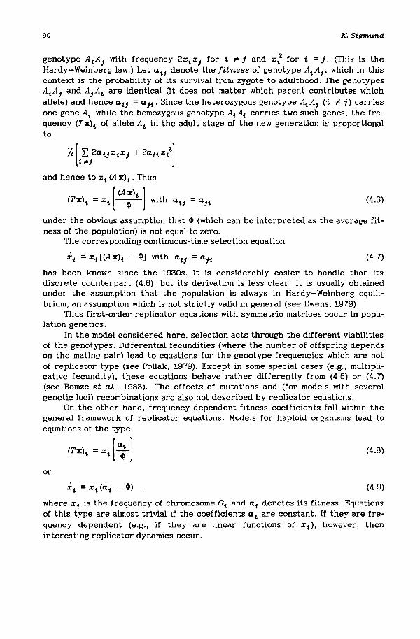
90 K. Sigmund

genotype AiAj with frequency 2xi x j for i ;t. j and x i2 for i = j. (This is the

Hardy-Weinberg law.) Let aij denote the fitness of genotype AiAj , which in thiscontext is the probability of its survival from zygote to adulthood. The genotypesAiA j and AjAi are identical (it does not matter which parent contributes whichallele) and hence aij = aji' Since the heterozygous genotype AiAj (i ;t. j) carriesone gene Ai while the homozygous genotype AiAi carries two such genes, the fre­quency (TX)i of allele Ai in the adult stage of the new generation is proportionalto

*[1: 2aijxixj + 2aHxl]i "j

and hence to xi (A X)i . Thus

[(A X)i] .

(Tx)i = xi --ep- wlth aij (4.6)

under the obvious assumption that ep (which can be interpreted as the average fit­ness of the population) is not equal to zero.

The corresponding continuous-time selection equation

xi =xi [(A x)i - ep] with aij =aji (4.7)

has been known since the 1930s. It is considerably easier to handle than itsdiscrete counterpart (4.6), but its derivation is less clear. It is usually obtainedunder the assumption that the population is always in Hardy-Weinberg equili­brium, an assumption which is not strictly valid in general (see Ewens, 1979).

Thus first-order replicator equations with symmetric matrices occur in popu­lation genetics.

In the model considered here, selection acts through the different viabilitiesof the genotypes. Differential fecundities (where the number of offspring dependson the mating pair) lead to equations for the genotype frequencies which are notof replicator type (see Pollak, 1979). Except in some special cases (e.g., multipli­cative fecundity), these equations behave rather differently from (4.6) or (4.7)(see Bomze et al., 1983). The effects of mutations and (for models with severalgenetic loci) recombinations are also not described by replicator equations.

On the other hand, frequency-dependent fitness coefficients fall within thegeneral framework of replicator equations. Models for haploid organisms lead toequations of the type

(Tx)i = Xi ( i ] (4.8)

or

(4.9)

where Xi is the frequency of chromosome Gi and a i denotes its fitness. Equationsof this type are almost trivial if the coefficients a i are constant. If they are fre­quency dependent (e.g., if they are linear functions of Xi)' however, theninteresting replicator dynamics occur.

A Survey qfRept1.c~torEqu~t1.o7l.s

Prebiotic evolution

91

Equations of type (4.8) were first studied (initially within the framework ofchemical kinetics) in an important series of papers by Eigen (1971) and Eigen andSchuster (1979) on prebiotic evolution. In this context the xi are the concentra­tions of self-replicating polynucleotides (RNA or DNA) in a well-stirred dialysisreactor with a dilution flow «P regulated in such a way that the total concentrationxl + ... + %71. remains constant (without loss of generality we can set this concen­tration equal to 1). In the absence of mutations this leads to continuous-time repli­cator equations (generation effects do not play any part, even if the initial popula­tion of molecules reproduces in some synchronized way).

Independent replication of the polymers leads to equations (4.8) with con­stant reproduction rates a1.' This implies (except in the case of kinetic degen­eracy) that all but one of the molecular species vanishes, with the loss of thecorresponding encoded information. In their search for ways of preserving the ini­tial amount of molecular information, Eigen and Schuster were led to study net­works of catalytically interacting polynucleotides. Such interactions (and thecorresponding replication rates) are usually quite complicated, but neverthelesssome rather general results have been obtained. In addition, certain special casesof linear catalytic (or inhibiting) interactions, yielding the first-order replicatorequations:

(4.10)

have been studied as approximations of more realistic chemical kinetics.The hypercycle (a closed feedback loop in which each molecular species is

catalyzed by its predecessor) has attracted particular attention (see Schuster etal., 1979, 1980; Hofbauer et al., 1980). Both the cooperation of the componentswithin a hypercycle and the strict competition between individual hypercyclessuggest that such networks may have been involved in some phases of early prebi­otic evolution. The hypercycle equation is given by

(4.11)

where the indices are taken on modulo n and the functions Hi (x) are strictly posi­tive on 871.' If the Hi are constants, k1.' the above equation then reduces to a spe­cial case of the first-order replicator equations:

Xi = Xi (k1. x 1. -1 - «P), k1. > 0

obtained if matrix A = (a1.j) in equations (4.10) is a permutation matrix:

fo 0 0 k 11

k z 0 0 0

0 kg 0 0

A =

0 0 k7l.-1 0

(4.12)

92

Animal behavior

K. S'tgmund

Taylor and Jonker (1978) were the first to introduce first-order replicatorequations into models of the evolution of animal behavior. This approach wasbased on Maynard Smith's use of game theory in the study of animal conflictswithin a species, equating strategies with behavioral phenotypes and payoffs withincrements of individual fitness.

These investigations initially centered on the notion of evolutionary stability(see Maynard Smith. 1974), which may be interpreted as game-theoretic equilibriawhich are proof against the invasion of behavioral mutants. This static approachassumed certain implicit dynamics which were soon made explicit in the form ofequations. once again of replicator type.

Let E 1 ,...•En denote the behavioral phenotypes within a population. x 1 •...• x nthe frequencies with which they occur, and aij (1 ~ i. j ~ n) the expected pay­off for an Ei-strategist in a contest against an Ej-strategist. Then, assuming ran­dom encounters, we obtain (A X)i as the average payoff for an Ei -strategist withina population in state x, and

(4.13)

as the mean payoff. In the case of asexual reproduction. the rate of increasexi / Xi of phenotype Ei is given by the difference (A x)i - x-A x. which once againyields (4.10) [or, in the discrete-time case,

[(A x)i + c]

(TX)i = xi if.l + C ' (4.14)

where C is a positive constant].The assumption of asexual reproduction at first seems rather unnatural. It

can be shown, however, that in many important examples the essential features ofthe dynamical model are preserved in the more complicated case of sexual repro­duction (see Maynard Smith, 1981; Hofbauer et al., 1982; Hines. 1980; Bornze et al.,1983; Eshel, 1982). Rather than introducing some sort of Mendelian machinerywhich, given the present state of knowledge of the genetic basis of behavior, isbound to be highly speculative, it seems reasonable to adhere to the more robustand manageable asexual model (see Schuster and Sigmund, 1984).

The corresponding replicator equations are examples of frequency­dependent sexual or asexual selection equations. Many specific types of conflict(e.g., the Hawk-Dove-Bully-Retaliator game, the War of Attrition game, and theRock-Scissors-Paper game) have been examined within this framework (see Zee­man, 1981; Bishop and Cannings, 1978; Schuster et al., 1981).

The game-dynamical aspects of the linear replicator equations (4.10) may beexpected to lead to applications in fields such as psychology and economics (seeZeeman, 1981). A justification of viewing strategies as replicators is given by Daw­kins (1982).

A Survey ofRepL1.cator Equat1.ons

Population ecology

Equations used to model ecological systems are commonly of the form

Y1. =Y1.!1.(Y1.···.Yn)' i =l.... ,n

93

(4.15)

(4.17)

(4.16)

= OJ with

where Y1. are the densities of different populations interacting through competi­tion, symbiosis, host-parasite. or predator-prey relationships. Such equations"live" on R: and are usually not of replicator type. However, relative densities doyield replicator equations. In particular, Hofbauer (1981a) has shown that theclassic (n -i)-species Lotka-Volterra equation

Y1. = Y1. (b1.n + "i:,b1.jYj)' i = 1, ....n-l

is equivalent to the first-order replicator equation (4.10) on Sn \ !x: x na1.j = b1.j - b1.n'

Y1.x1. = -'11.--' i =l..... n

l: Yjj=l

and Y n == 1. The barycentric transformation (4.17), together with a change in velo­city, maps the orbits of equations (4.16) into the orbits of equations (4.10). Whichof these equations is more convenient will depend on the problem considered. Simi­lar results hold for interactions of order higher than linear.

Sexually reproducing organisms are not replicators in the strict sense of theterm, but within ecological considerations and disregarding genotypes they may beviewed as such.

General Properties

The term 41 in equation (4.3) guarantees that the continuous-time replicatorequations (4.10) "live" on Sn' since (l:x1.) =0 on Sn' Thus. the simplex and all itsfaces (which consist of subsimplices characterized by x1. = 0 for all i in some non­trivial subset I of {l. ....n l> are invariant. In particular, the corners e1. are equili­bria. The solutions of equations (4.1) in Sn are defined for all t E: R

For the discrete-time replicator equation (4.2) to have any meaning. the term41 must be nonvanishing on Sn' It always has the same sign and we assume that the! 1. (x) are also of this sign. say positive. In this case the simplex and all of itsfaces are once again invariant. If a continuous- or discrete-time replica tor equa­tion is restricted to a face of Sn the resulting equation is again of replicator type.

We say that two vector fields rand g on Sn are equivalent if there exists afunction c : Sn ... R such that!1. (x) - g1. (x) = C (x) holds on Sn for all i. If rand gare equivalent then the restrictions x1. = x1. [f1. (x) - rp] and X1. = x1. [g1. (x) - 41]coincide on Sn' In the same way. if there exists a function c : Sn ...R+ such that! 1. (x) = C (x)g1. (x) holds on Sn for all i. then the difference equations x ... Tx with(Tx)1. =x1.! 1. (X)rp-l and (Tx)1. =x1. g 1. (x)rp-1 coincide on Sn'

In particular, we say that the n xn matrices A and B are equivalent if thevector fields A x and Bx are equivalent in the sense described above. This is the

94 K. Sigmund

(4.19)

case if and only if there exist constants C j such that a ij - bij =C j for all i andj. Equivalent matrices lead to identical first-order replicator equations. Thus,without loss of generality. we may consider only matrices with zeros in the diago­nal, for example, or matrices whose first row vanishes.

Another useful property is the quotient rule

[:: r= [:;] [fi(x) -fj(x)] (4.18)

or, in the discrete case.

~~:~; = [:; ][~; ]

for x j > O.Losert and Akin (1983) have shown that the discrete-time first-order replica­

tor equation induces a diffeomorphism from Sn into itself. This result is importantbecause it excludes the chaotic behavior caused by the noninjectivity of mappingssuch as x .... ax(l-x). However, the discrete case is still far less well-understoodthan the continuous one and may behave quite differently.

Equilibria and Their Stability

The fixed points of equations (4.1) or (4.2) in the interior of Sn are thestrictly positive solutions of

and

f 1 (x) =... =f n (x)

Xi + ... + X n =1 .

(4.20)

(4.21)

If equation (4.20) holds, the common value is cPo Similarly, the equilibria in the inte­rior of a face defined by xi =0 for some i E: !l, .... n l are the strictly positivesolutions of the analogous equations.

In particular, the inner equilibria of first-order replicator equations are thestrictly positive solutions of the linear equations (4.21) and

(4.22)

These solutions form a linear manifold. Generically. there is either one or no inte­rior equilibrium. In fact. there is an open, dense subset of n x n matrices suchthat the corresponding replicator equations admit, at most. one fixed point in theinterior of Sn and in the interior of each face (Zeeman, 1980).

In many cases it is easy to perform a local analysis around a fixed point p bycomputing the eigenvalues of its Jacobian. One such eigenvalue is cP(p); thiscorresponds to an eigenvector p which is not in the tangent space. Since we arestudying the restriction of equations (4.1) to Sn' this eigenvalue (or more pre­cisely, one of its multiplicities) is irrelevant. Thus. for example, the relevanteigenvalues of a corner e i are the n -1 values of aij -aii (j "F i).

For the hypercycle (4.12) there is always a unique fixed point p in intsn ,which is given by

A Survey ofRept1.cator Equat1.ons 95

k -11.

P1. = 2: k j- 1

and the eigenvalues of the Jacobian at p are (up to a positive factor) the nthroots of unity, except for 1 itself (see Schuster et al., 1980). It follows that pisasymptotically stable for n ,..;; 3 and unstable for n ~ 5. In fact, using IT%1. as aLjapunov function, it can be shown that p is globally stable for n ,..;; 4. For n ~ 5,numerical computations show that a periodic attractor exists, although this hasnot been proved rigorously.

Linearization around the inner equilibrium of equations (4.12) allows the useof the Hopf bifurcation technique. Zeeman (1980) has shown that for n = 3 suchbifurcations are degenerate and do not lead to periodic attractors. In fact, theequivalence of equation (4.10) for n =3 with the two-dimensional Lotka-Volterraequation (4.16) implies that it admits no isolated periodic orbit. For n ~ 4, how­ever, there exist nondegenerate Hopf bifurcations, the simplest of which is givenby

0 1 -JJ. o 10 0 1 -JJ.

-JJ. 0 0 11 -JJ. 0 0

which, for JJ. =0, reduces to the hypercycle equation with globally stable interiorequilibrium (see Hofbauer et al., 1980). De Carvalho (1984) refined this by showingthat for small JJ. > 0, the periodic orbit is globally attracting in intSn , except forthe stable manifold of the inner equilibrium.

If there is no fixed interior point, then there exists acE: R n with l:c1. =0

such that the function IT%~( (which is defined on intSn ) increases along the orbitsof equation (4.10) (Akin, 1980; Hofbauer, 1981b). It follows from Ljapunov'stheorem that each orbit x(t) in the interior of Sn has its c.> limit

c.>(x) =!y E: Sn : 3 t n .... +00 with x(tn ) .... y!contained in the boundary of Sn' This implies that there are no periodic, orrecurrent, or even nonwandering points in intsn if there is no fixed inner point.However, this does not mean that lim t -++00%1. (t) =0 for some i. Akin and Hofbauer(1982) give an example, with n =4, where the c.> limit of every interior orbit is acycle consisting of the corners 11., ez, ~, e4 , and the edges joining them. Con­versely, if the orbit x(t) is periodic in intSn or, more generally, has its c.> limit inintsn , then the time averages of this orbit

T

lim 1-J%1. (t )dt, i =1,oo.,n (4.23)T-++ooT 0

exist and correspond to an interior equilibrium of equations (4.10) (see Schusteret al., 1980). It frequently happens that an interior equilibrium is unstable andhence physically unattainable, but is nevertheless still empirically relevant as atime average.

96

Per:manence

K. Sigmund

It is often very difficult to derive a full description of the attractors ofreplicator equations. [Recall that strange attractors have been observed numeri­cally (Arneodo et al., 1980), and that there is still no proof of the existence of aunique limit cycle for the hypercycles (4.12) with n ~ 5]. More modest resultsmay be obtained in such situations by considering only whether the attractors arein the interior or on the boundary.

In particular, we say that the replicator equations (4.1) are permanent ifthere is a compact set in intSn which contains the (.) limits of all orbits starting inintSn [or, equivalently, if there is a 0 > 0 such that lim t ..+.. infx i (t) ~ 0 for all i,whenever xi (0) > 0 for all i]. Such systems are robust in a sense which is obvi­ously of great practical importance in ecology, genetics. or chemical kinetics. Onthe one hand, the state remains bounded at some distance from the boundary evenif it oscillates in some regular or irregular fashion: therefore a population (or com­ponent) within this system cannot be wiped out by small fluctuations. On theother hand, if the system starts on the boundary (Le.. with one or more com­ponents missing), then mutations introducing these components (even if only intiny quantities) spread, with the result that the system is soon safely cushionedaway from the faces of the simplex.

We must make two remarks here. First, permanence is not a stnIcturallystable property (in the same way that the asymptotic stability of a fixed point isnot necessarily structurally stable). Second, a nonpermanent system does notalways lead to the exclusion of some components. Zeeman (1980) has shown thatthere is a specific case of equation (4.10) which has an attractor on the boundaryand one in the interior. It can also happen that each interior orbit remainsbounded away from the faces, but by a threshold which depends on the orbit; forpermanence, the threshold must be uniform.

The most useful sufficient condition for permanence is the existence of afunction P .defined on Sn' with P(I) > 0 for I E: intSn and P(I) = 0 for I E: bdSn ,such that P = P~, where Y is a continuous function with the property that, for allI E: bdSn , there is some T > 0 such that

T

~JY[I(t )]dt > 0 . (4.24)o

We describe P as an average Ljapunov function. Near the boundary, Pincreases on average, so that the orbits move away from the boundary (Hofbauer,1981b).

It has been shown by Schuster et al. (1981) and by Hofbauer (1981b) that thegeneral hypercycle equations (4.11) have P(I) = x 1X 2'" X n as an averageLjapunov function and are therefore permanent. This is of great importance in therealistic design of catalytic hypercycles, whose dynamics are too complex to berepresented by equations (4.12).

Brouwer's fixed point theorem implies that a necessary condition for per­manence is the existence of a fixed point in intSn (Hutson and Vickers, 1983). Forpermanent first-order replicator equations (4.10), such an equilibrium is neces­sarily unique. Another very useful condition for the permanence of equations(4.10) is that the trace of the Jacobian at this fixed point must be strictly nega­tive (Amann and Hofbauer, 1984).

A Survey 01RepLicator Equations

Amann and Hofbauer obtained a remarkable characterization of permanencefor systems (4.10) with matrices A of the form

[0

+ 0+ 0

. + 0

where + means that the corresponding element is strictly positive and - meansthat it is negative or zero. The following conditions are equivalent for equations ofthis type:

(-1) The system is permanent.(2) There is a unique inner equilibrium p and ~(p) is strictly positive.(3) There is a vector Z E: Rn , with zi > 0 for all i, such that all components of

zA are strictly positive.(4) The matrix C obtained from A by setting cii =a i +1,i (taking indices of

modulo n), that is, by moving the first row to the bottom, is such that itsdeterminant and all its principal minors are strictly positive.

Note that -~(p) is just the trace of the Jacobian at p and that matrices suchas C, which have diagonal terms strictly positive and all other terms nonpositive,play an important role in mathematical economics.

As a special case we find that the hypercycle equation (4.12) is always per­manent. Another special case has been obtained by Zeeman (1980): the replicatorequation (4.10) with n = 3 and A of the form

[0 + -1

l-0 +j+ - 0

is permanent if and only if detA > 0 (in this case the inner equilibrium is a globalattractor). In addition, Amann and Hofbauer (1984) have used the general theoremto characterize permanence in special types of reaction networks, such as hyper­cycles of autocatalysts:

:i: = Xi (aix i + bi -1Xi -1 - ~) (4.25)

or superpositions of counter-rotating hypercycles:

(4.26)

with (a i ,bi > 0). Hofbauer (1981b) has also proved that inhomogeneous hyper­cycles

(4.27)

98 K. Stgmund

with at > O. are permanent if they have an interior equilibrium. This was done-1

using TIx:' as an average Ljapunov function. More generally, Hofbauer conjec-tures that equation (4.10) is permanent if and only if for some p with Pt > O. the

function TIxfi is an average Ljapunov function or, equivalently, if and only if forsuch a p the inequality p·A x > x·A x holds for all fixed points x in bdSn . This wasproved by Amann (1984) for the case n = 4.

It can be shown that a necessary condition for the permanence of first-orderreplicator equations with a tj ~ 0 is that an irreducible graph is obtained on draw­ing an arrow from j to i wherever a tj > 0; that is, that any two vertices can bejoined by an oriented graph (see Sigmund and Schuster. 1984). It would beinteresting to know if such a graph is necessarily Hamiltonian; that is. contains aclosed oriented path visiting each vertex exactly once. [This has been shown byAmann (1984) for the case n ~ 4 and att = 0.]

An interesting class of examples is provided by models describing the com­petition between several hypercycles. If these hypercycles are disjoint then theequation is of the form

(4.28)

where 11' is a permutation of indices containing several cycles. Such systems arenot irreducible and hence not permanent. If the cycles are all of length less than4, then one of them succeeds and the others vanish (see Schuster et al., 1980).This is probably also true for larger cycles, but has not yet been proved.

Once again. the situation is much less clear in the case of discrete-time repli­cator equations. A sufficient condition analogous to the existence of an averageLjapunov function has been given by Hutson and Moran (1982). Hofbauer (1984)has shown that the discrete hypercycle

(Tx)t =xt [kt Xt ;l +c] (4.29)

(with k t > 0) is permanent if and only if C > o.

Gradient Systems of Replicator Type

The evolutionary dynamics defined by the gradients of certain potentialfunctions are of great interest because they correspond to popular notions ofadaptive genotypic or phenotypic landscapes and yield biological models withextremum principles of a type familiar in theoretical physics. The action of selec­tion in such situations drives the state uphill along the path of steepest ascent.

Gradients depend on metrics. Shahshahani (1979) provided a geometricframework for population dynamics by using a Riemann metric instead of the moreusual Euclidean metric on S"". Replicator equations which are gradients withrespect to this metric are of considerable interest (see Akin, 1979).

Shahshahani defines the inner product of two vectors x and y in the tangentspace 1j, S"" (where p E ints",,) in the following way:

1<x.Y>p = 'E- xtYtPt

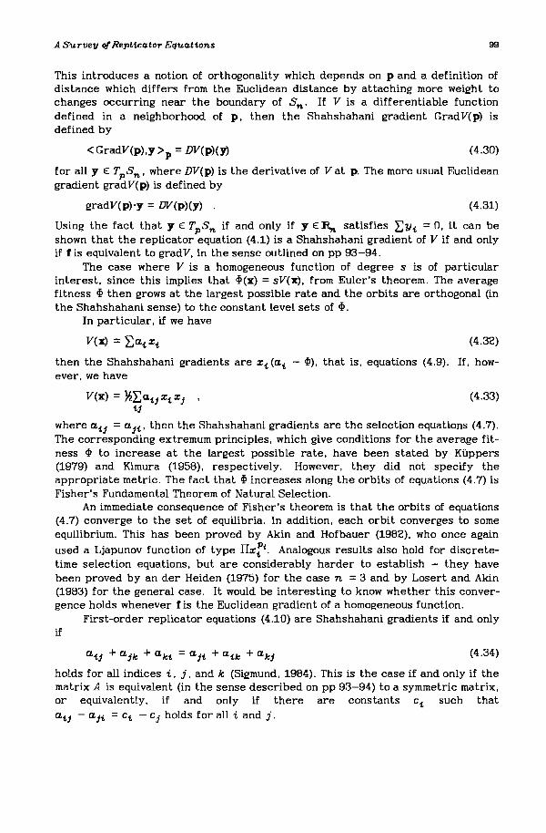
A Survey 0/RepL1.ca.tor Equa.tions 99

This introduces a notion of orthogonality which depends on p and a definition ofdistance which differs from the Euclidean distance by attaching more weight tochanges occurring near the boundary of Sn' If V is a differentiable functiondefined in a neighborhood. of p, then the Shahshahani gradient GradV(p) isdefined by

< GradV(p),y >p = DV(p)(y) (4.30)

for all y E: TpSn , where DV(p) is the derivative of Vat p. The more usual Euclideangradient gradV(p) is defined by

gradV(p)-y = DV(p)(y) . (4.31)

Using the fact that y E: Tps'", if and only if y E: R,.. satisfies L;y1. =0, it can beshown that the replicator equation (4.1) is a Shahshahani gradient of V if and onlyif r is equivalent to gradV, in the sense outlined on pp 93-94.

The case where V is a homogeneous function of degree s is of particularinterest, since this implies that CP(x) = sV(x). from Euler's theorem. The averagefitness cp then grows at the largest possible rate and the orbits are orthogonal (inthe Shahshahani sense) to the constant level sets of CP.

In particular, if we have

V(x) = 'Ea1. xi (4.32)

then the Shahshahani gradients are xi (a1. - CP), that is, equations (4.9). If, how­ever, we have

V(x) = *L:a1.j xi x j (4.33)1.j

where a1.j = a j 1.' then the Shahshahani gradients are the selection equations (4.7).The corresponding extremum principles, which give conditions for the average fit­ness cP to increase at the largest possible rate, have been stated by Kilppers(1979) and Kimura (1958), respectively. However, they did not specify theappropriate metric. The fact that cP increases along the orbits of equations (4.7) isFisher's Fundamental Theorem of Natural Selection.

An immediate consequence of Fisher's theorem is that the orbits of equations(4.7) converge to the set of equilibria. In addition, each orbit converges to someequilibrium. This has been proved by Akin and Hofbauer (1982), who once again

used a Ljapunov function of type ITxf'. Analogous results also hold for discrete­time selection equations, but are considerably harder to establish - they havebeen proved by an der Heiden (1975) for the case n = 3 and by Losert and Akin(1983) for the general case. It would be interesting to know whether this conver­gence holds whenever r is the Euclidean gradient of a homogeneous function.

First-order replicator equations (4.10) are Shahshahani gradients if and onlyif

a1.j + a jk + a ki = a j 1. + a1.k + a kj (4.34)

holds for all indices i, j, and k (Sigmund. 1984). This is the case if and only if thematrix A is equivalent (in the sense described on pp 93-94) to a symmetric matrix,or equivalently, if and only if there are constants c1. such thata1.j - aji = c1. - Cj holds for all i and j.

100

Equations of the type

X1. = %1. [g1. (%1.) - Ill]

K.S1.gmunct

(4.35)

are obviously Shahshahani gradients. If the functions g1. are monotonicallydecreasing, they model competition between replicators which inhibit their owngrowth but are otherwise independent. In this case it can be shown that thereexists a unique global attractor. More precisely, we can assume without loss ofgenerality that g 1 (0) ~ g 2(0) ~ ... ~ gn (0) > 0, in which case there exists anumber K and apE: Sn such that

gl<P 1) = ... = gm<Pm ) = K

Pi > O.···.Pm > 0, P m +1 =O, ... ,Pn =0

(4.36)

(4.37)

where m is the largest integer i with g j (0) > K. The point p is the limit. as tapproaches +00, of all orbits x(t) for which %1. (0) > 0, i = 1 •... ,m. A variant of thismodel shows that if the total concentration l;%1. is kept at a constant value c (notnecessarily equal to 1) by replacing <P by Illi c, then the number of species thatcan coexist increases with increasing c (see Hofbauer et al.. 1981). The specialcases

(4.38)

have been studied by Epstein (1979).

Classification

Except in low-dimensional cases. there is little hope of obtaining a completeclassification of first-order replicator equations (4.10) up to topologicalequivalence. Two such equations are said to be topologically equivalent if thereexists a homeomorphism from Sn onto itself which maps the orbits of one equationonto the orbits of the other equation in such a way that orientation is preserved.Two n x n matrices are described as R-equivalent if the corresponding replicatorequations are topologically equivalent.

Zeeman (1980) proposed a method for the classification of stable cases. Byanalogy to the definition of structural stability, an n Xn matrix A is said to bestable if its R-equivalence class is a neighborhood of A. Thus, small perturbationsof A do not change the top'ological structure of the corresponding replicator equa­tion. Zeeman conjectured that the stable matrices form an open dense set in thespace of n x n matrices and are divided into a finite number of R-equivalenceclasses for each n. He proved this for n = 2 and 3, and classified all correspond­ing stable replicator equations. (For n = 2 and 3 there are 2 and 19 stableclasses. respectively, up to time reversal.)

A basic requirement for the classification of equation (4.10) for n = 3 is thatthere are no limit cycles. This is a consequence of the corresponding result fortwo-dimensional Lotka-Volterra equations (see. e.g.• Coppel, 1966) and of theequivalence between such equations and first-order replicator equations(Hofbauer. 1981a). Bomze (1983) extended Zeeman's classification to coverunstable cases. obtaining 102 types of phase portraits up to time reversal.

Little is known about stable matrices for higher dimensions. apart from thefact that stability implies that all fixed points of equations (4.10) are hyperbolic

A SUMJey qfRepttcator Equat1.o""s 101

(the real parts of the eigenvalues of their Jacobians do not vanish). This wasproved by de Carvalho (1984).

Recall that, without loss of generality, the diagonal of a matrix may beassumed to contain only zeros. Let Z"" denote the class of such matrices withnonzero off-diagonal terms. Two matrices A and B in Z"" are said to be signequivalent if the corresponding off-diagonal terms have the same sign and com­binatorially equivalent if A can be made sign equivalent to B by permutatingthe indices. Zeeman (1980) showed that A and Bare combinatorially equivalent ifand only if the equations obtained by restricting the corresponding replicatorequations to the edges of S"" are topologically equivalent. Within Z"", R-equivalenceclasses are refinements of the combinatorial classes. There are 10 such combina­torial classes for n = 2 and 114 for n = 3 up to sign reversal (Zeeman, 1980). DeCarvalho (1984) has studied 19 combinatorial classes without inner equilibria as afirst step towards a classification of R-stable matrices for n =4. Another step inthis direction was taken by Amann (1984), who characterized all 4 x 4 matriceswhich lead to permanent replicator equations.

Another interesting (although highly degenerate) class of examples is pro­vided by circulant matrices (a1.J =at +l,J +1 for all i and j, counting indices onmodulo n). A partial analysis of this class is given in Hofbauer et al. (1980). It isshown that the center of S"" (Le .. the point m, where m1. =1/ n) is always anequilibrium; it is not hard to compute the eigenvalues of its Jacobian. If m is asink, then m is a global attractor; if m is a source, then all orbits converge to theboundary. Nondegenerate Hopf bifurcations occur for n ~ 4.

Connections with Game Theory

It has often been remarked that game theory is essentially static. However,the replicator equations (4.10) and (4.14) offer dynamic models for normal formgames which are symmetric in the sense that both players have the same stra­tegies and the same payoff matrix A. In fact, the dynamic extension is alreadyimplicit in the notion of an evolutionarily stable state (Maynard Smith, 1974, 1982),which is a refinement of the concept of a Nash equilibrium.

A point p E: S"" is said to be evolutionarily stable if it satisfies the followingtwo conditions:

(1) Equilibrium condition:

p-Ap ~ x-A p for all x E: S""

(2) Stability condition:

if p-Ap = x-Ap for x ~ p, then p·Ax > x·Ax .

(4.39)

(4.40)

A game can have zero, one, or several evolutionarily stable points. As shown bySelten (1985), the notion is not structurally stable: some matrices which yield evo­lutionarily stable points can be perturbed into matrices which do not. In this con­text we also refer the reader to Bomze (1985) for a thorough analysis of the rela­tion of evolutionary stability to the multitude of equilibrium concepts used in gametheory.

102 K. Sigmund

It can be shown that the following four conditions are equivalent (seeHofbauer et al., 1979; Zeeman, 1980):

(1) P is evolutionarily stable.(2) For all q E: Sn with q '" p, we have

p-A [(1 - e)p + eq] > q-A [(1 - e)p + eq]

provided that e > 0 is sufficiently small.(3) For all x'" p in some neighborhood of p, we have

p-Ax > x-Ax.

(4.41.)

(4.42)

(4) The function IIxfi is a strict local Ljapunov function at p for the replicatorequations (4.10); that is, strictly increasing along all orbits in a neighborhoodof p.

Condition (2) is probably the most intuitively obvious in a biological context:if the state of the population is p, then a fluctuation introducing a small subpopu­lation in state q becomes extinct, since the p population fares better than the qpopulation against the mixture (1 - e)p + eq.

It follows from the equivalence of (1) and (4) that any evolutionarily stablepoint p is an asymptotically stable fixed point of equations (4.10). However, theconverse is not true. In particular, (3) implies that if p E: intSn is evolutionarilystable, then it is an attractor for all orbits in intSn , and hence the unique evolu­tionarily stable point in Sn; however, Zeeman (1980) has shown that there exist3 x3 games with two asymptotically stable fixed points, one in the interior and theother on the boundary of Sn .

Akin (1980) has shown that equations (4.10) have no fixed point in intSn ifand only if there exist two strategies x and yin Sn such that x dominates y in thesense that

x·Az > y-Az

for all Z E: intSn . This result is supplemented by precise statements concerningthe support of strategies x and y and the form of global Ljapunov functions orinvariants of motion for equations (4.10).

The results obtained using the time averages (4.23) described on p 95 suggesta computational method for finding equilibria (and hence solutions) of normal formgames. These results, which can easily be extended to asymmetric games (Le.,games in which the players have different payoff matrices), should be comparedwith the classical methods (involving differential equations) for finding the solu­tions of games (see, e.g., Luce and Raiffa, 1957, p. 438).

The discrete analogues of such methods involve iterative procedures. It turnsout, however, that discrete-time replicator equations of the type (4.14) do notappear to lend themselves very well to game dynamics; in particular, an evolu­tionarily stable point need not be asymptotically stable for equations (4.14) (see,e.g., Schuster and Sigmund, 1984).

The behavior of equations (4.10) and (4.14) for zero-sum games (aij = -a ji ) isanalyzed in Akin and Losert (1984). If an interior equilibrium exists, then the con­tinuous model (4.10) has an invariant of motion. The equilibrium is stable, but notasymptotically stable, and all nonequilibrium orbits of model (4.10) in intSn have CJ

A Survey ofRepLica.tor Equa.tions 103

limits in intSn but do not converge to an equilibrium. By contrast, if the discretetime model (4.14) has an interior equilibrium then it is unstable and all nonequili­brium orbits converge to the boundary. If there is no inner equilibrium, then allorbits converge to the boundary in both discrete and continuous cases. In thediscrete case all possible attractors may be described using the notion of chainrecurrence.

References

Akin, E. (1979) The geomet.ry of population genetics. Lecture Notes In Biomathematics31 (Berlin, Heidelberg, and New York: Springer-Verlag).

Akin, E. (1960) Domination or equilibrium. Math. Biosciences 50: 239-50.Akin, E. and Hofbauer, J. (1962) Recurrence of t.he unfit.. Math. Biosciences 61: 51-63.Akin, E. and Losert., V. (1964) Evolutionary dynamics of zero-sum games. J. Math. Biol-

ogy 20: 231-56.Amann, E. (1964). Permanence for Catalytic Networks. Dissert.ation (Universit.y of

Vienna).Amann, E. and Hofbauer, J. (1965) Permanence in Lot.ka-Volt.erra and replicat.or equa­

tions. Fort.hcoming.Arneodo, A., Coullet., P., and Tressor, C. (1960) Occurrence of st.range at.t.ract.ors in

t.hree-dimensional Volt.erra equations. Physics Letters 79A: 259-63.Bishop, T. and Cannings, C. (1976) A generalized war of at.t.rition. J. Theor. Biology 70:

65-124.Bomze, 1. (1963) Lot.ka-Volt.erra equat.ions and replicat.or dynamics: a t.wo-dimensional

classification. Biol. Cybernetics 46: 201-11.Bomze, 1. (1965) Non-cooperative t.wo-person games in biology: symmet.ric cont.est.s, in

Peschel (Ed) Lotka-Volterra Approach in Dynamical Systems, Proc. Conf. Wart.­bury (Berlin: Akademieverlag).

Bomze, 1., Schust.er, P., and Sigmund, K. (1963) The role of Mendelian genetics in st.ra­t.egic models on animal behavior. J. Theor. Biology 101: 19-36.

de Carvalho, M. (1964) Dynamical S'ystems ana Game Theory. PhD Thesis (Universit.y ofWarwick).

Coppel, W. (1966) A survey of quadratic syst.ems. J. [)iff. Eqns. 2: 293-304.Dawkins, R. (1962) The E:r:tenaea Phenotype (Oxford and San Francisco: Freeman).Eigen, M. (1971) Self-organization of mat.t.er and t.he evolution of biological macro­

molecules. Die Naturwissenscha,tten 56: 465-523.Eigen, M. and Schust.er, P. (1979) The Hypercycle: A Principle Of Natural Se1.f­

Organization (Berlin and Heidelberg: Springer-Verlag).Epst.ein, M. (1979) Competit.ive coexist.ence of self-reproducing macromolecules. J.

Theor. Biology 76: 271-96.Eshel, 1. (1962) Evolutionarily st.able st.rat.egies and nat.ural selection in Mendelian popu­

lat.ions. Theor. Pop. Biol. 21: 204-17.Ewens, W.J. (1979) Mathematical Population Genetics (Berlin, Heidelberg, and New

York: Springer-Verlag).an der Heiden, U. (1975) On manifolds of equilibria in t.he selection model for multiple

alleles. J. Math. Biol. 1: 321-30.Hines, G. (1960) An evolutionarily stable st.rat.egy model for randomly mat.ing diploid

populations. J. Theor. Biology 67: 379-64.Hofbauer, J. (1961a) On t.he occurrence of limit. cycles in t.he Volt.erra-Lot.ka equation.

Nonlinear Analysis IMA 5: 1003-7.Hofbauer, J. (1961b) A general cooperation t.heorem for hypercycles. Monatsh. Math.

91: 233-40.Hofbauer, J. (1964) A difference equation model for t.he hypercycle. SIAM J. Appl. Math.

44: 762-72.

104 K. Sigmund:

Hofbauer, J., Schuster, P., and Sigmund, K. (1979) A note on evolutionarily stable stra­tegies and game dynamics. J. Theor. Biology 81: 609-12.

Hofbauer, J., Schuster, P., Sigmund, K.. and Wolff, R. (1980) Dynamical systems underconstant organization. Part 2: Homogeneous growth functions of degree 2. SlAM J.Appl. Math. 38: 282-304.

Hofbauer, J., Schuster, P., and Sigmund, K. (1981) Competition and cooperation in cata­lytic self-replication. J. Math. Biol. 11: 155-68.

Hofbauer, J., Schuster. P., and Sigmund, K. (1982) Game dynamics for Mendelian popula­tions. Biol. Col/bern. 43: 51-7.

Hutson, V. and Moran, W. (1982) Persistence of species obeying difference equations. J.Math. Biol. 15: 203-13.

Hutson, V. and Vickers, C.T. (1983) A criterion for permanent coexistence of species,with an application to a two-prey/one-predator system. Math. Biosci. 63: 253-69.

Kimura, M. (1958) On the change of population fitness by natural selection. Hered.ity12:145-67.

Kiippers, B.a. (1979) Some remarks on the dynamics of molecular self-organization.Bull. Math. Biol. 41: 803-9.

Losert, V. and Akin, E. (1983) Dynamics of games and genes: discrete versus continuoustime. J. Math. Biol. 17: 241-51.

Luce, R. and Raiffa, H. (1957) Games and. Decisions (New York: John Wiley).Maynard Smith, J. (1974) The theory of games and the evolution of animal conflicts. J.

Theor. Biology 47: 209-21.Maynard Smith, J. (1981) Will a sexual population evolve to an ESS? Amer. Naturalist

177: 1015-8.Maynard Smith, J. (1982) Evolutionary Game Theory (Cambridge: Cambridge University

Press).Pollak, E. (1979) Some models of genetic selection. Biometrics 35: 119-37.Schuster, P. and Sigmund, K. (1983) Replicator dynamics. J. Theor. Biology 100: 535-8.Schuster, P. and Sigmund, K. (1985) Towards a dynamics of social behavior: strategic

and genetic models for the evolution of animal conflicts. J. Soc. Biol. Structures.Forthcoming.

Schuster, P., Sigmund, K., and Wolff, R. (1979) Dynamical systems under constant organi­zation. Part 3: Cooperative and competitive behavior of hypercycles. J. Di.f1.Eqns. 32: 357-68.

Schuster, P., Sigmund, K., and Wolff, R. (1980) Mass action kinetics of self-replication inflow reactors. J. Math. Anal. Appl. 76: 66-112.

Schuster, P., Sigmund, K., Hofbauer, J., and Wolff. R. (1981) Self-regulation of behaviorin animal societies. Part 1: Symmetric contests. Biol. Cybern. 40: 1-6.

Shahshahani, S. (1979) A new mathematical framework for the study of linkage and selec­tion. Memoirs AMS 211.

Selten, R. (1965) Evolutionary stability in extensive two-person games. Math. Soc. Sci­ences. Forthcoming.

Sigmund, K. (1965) The maximum principle for replicator equations, in Peschel (Ed)Lotka-Volterra Approach in Dynamical Systems, Proc. Conf. Wartburg (Berlin:Akademieverlag).

Sigmund, K. and Schuster, P. (1984) Permanence and uninvadability for deterministicpopulation models, in P. Schuster (Ed) stochastic Phenomena and. ChaoticBehavior in Complez Systems (Berlin, Heidelberg, and New York: Springer­Verlag).

Taylor, P. and Jonker, L. (1976) Evolutionarily stable strategies and game dynamics.Math. Biosciences 40: 145-56.

Zeeman, E.C. (1960) Population dynamics from game theory, in Global Theory ojDynam­ical Systems, Lecture Notes in Mathematics 619 (Berlin, Heidelberg, and NewYork: Springer-Verlag). .

Zeeman, E.C. (1961) Dynamics of the evolution of animal conflicts. J. Theor. Biology 89:249-70.

CHAPTERS

Daminian Evolution in Ecosystems:A Survey of Some Ideas and DifficultiesTogether with Some Possible Solutions

Nils Chr. Stenseth

Introduction

Ecology, the biological science of environment, has not produced a synthesisof environment from its broad technical knowledge of influence of externalparameters on organisms. Before Darwin (1859), environment was consideredan organic whole. Everything in it made some contribution and has somemeaning with respect to everything else. Darwin subscribed to this view, buthis emphasis, and that of his followers, on the evolving organism struggling tosurvive, suppressed the exploration of holistic aspects of the origin ofspecies that might have been developed. After Darwin, the organism cameinto great focus, first as a comparative anatomical entity, then later withphysiological, cellular, molecular, behavioural, and genetic detail. In con­trast, the organism's environment blurred through relative inattention into afuzzy generality. The result was two distinct things (dualism), organism andenvironment, supplanting the original unified organism-environment whole(synergism). (Patten, 1982).

In a way we may say that we have two types of

... ecologies today, reflecting the tension between dualism and synergism.Population ecology, descended from Darwin, focuses on organism, and ecosys­tem ecology, in the earlier holistic tradition, deals with environment. Meldingof these two subdisciplines depends on finding the means to investigate theorganism-environment complex ... (Patten, 1982).

The Avstralian physicist and father of statistical mechanics, Ludwig E. Boltzmann,is reported (see, e.g., Maynard Smith, 1982a) to have said that the nineteenth cen­tury probably would be remembered as Darwin's Century. More than one hundredyears after the death of Charles Darwin, Boltzmann seems to be right: today weremember Darwin as the person who convinced us that evolution is a fact and asthe person who presented a theory - consistent with the facts - which explained

106 N. Ch.T. Stenseth.

the mechanism of evolution, the process of natural selection. Thus, we mean byDarwinism the theory that evolution has occurred as a result of natural selec­tion. As the above quotations from Patten (1982) show, the influence of Darwin hasnot been only positive - it lead to dualism by focusing on the individual organismrather than the mutual interaction between the organism and the environment.Nevertheless, Darwin has, of course, had a tremendously positive influence onbiology - he made us understand how organisms evolve in a fixed environmentalsetting.

What Darwin (1859) did was to transform biology into a proper science with atheoretical basis, without which the study of biology would be nothing more thanan enterprise of collecting curiosa - it would be stamp collecting. The idea ofnatural selection has helped us to organize both our data and our thoughts as tohow the living world came to be like it is today. Darwin was also one of a series ofscientists who documented that our own species, Homo sapiens, was closelyrelated - phylogenetically - to other living creatures of the Earth; man no longerhad a unique position totally separate from all other organisms.

More than one hundred years after Darwin's death and after a long period ofheavy criticism and scrutiny, the basic ideas of Darwinism still hold. Muchremains, of course, to be done in the refinement of the Darwinian theory of evolu­tion. For example, one serious difficulty is that we do not understand what reallygenerates "selective pressure".

In this chapter I present the basic ideas in the Darwinian theory of evolu­tion, concentrating on the general ideas rather than providing a detailed review ofthe mathematical formulation and the empirical tests of this theory; good reviewsof both these aspects are already available (see, e.g., Roughgarden, 1979;Futuyma, 1979). Indeed, I want to concentrate on those aspects of Darwinismwhich, to my mind, are inappropriately treated in the literature. In the latterpart of the chapter I discuss some of the difficulties we are faced with when try­ing to formulate a theory as to how selective pressure is generated. Specifically, Ioutline some of the mathematical difficulties, but I also discuss some possiblemathematical fragments useful to a theory of evolution in ecosystems.

Evolution

Microevolution, macroevolution, and phylogenetics

The idea of a changing universe has now replaced the long unquestioned viewof a static world, identical in all essentials to the creator's perfect creation.Darwin more than anyone else extended to living things, and to the human speciesitself, the notion that mutability, not stasis, is the natural order. He suggestedthat material causes are a sufficient explanation not only for physical phenomena,as Descartes and Newton already had shown, but also for biological phenomena,with all their seeming evidence of design and purpose: it was no longer necessaryto refer to the will of God or to the Aristotelian final causes. As Futuyma (1979)points out,

... by coupling undirected, purposeless variation to the blind. uncaring pro­cess of natural selection, Darwin made theological or spiritual explanationsof the life processes superfluous. Together with Marx's materialistic theory

Darwinian EvoLution in Ecosystems

of history and society and Freud's attribution of human behaviour to influ­ences over which we have little control, Darwin hewed the final planks of theplatform of mechanism and materialism.

107

Evolution, the process of changing biological structures over time, is commonlydivided into two (partly overlapping) types: micro- and macro-evolution. Bymicroevolution we mean the patterns of change that occur within a species and bymacroevolution we usually mean evolution above the species level; herein, I usemacroevolution to refer to the processes of speciation and species extinction.

Darwin held that both micro- and macro-evolution could be understood asresulting from the same process. Hence, current Darwinists hold that macroevolu­tion may be seen as the sum of microevolutionary changes. About this presumptionthere has recently been much debate and disagreement; this I return to later.

Phylogenetics is the discipline that attempts to reconstruct the genealogicalrelationships of living and extinct organisms; from such studies phylogenetic treesare constructed. These phylogenetic trees are, by definition, assumed to indicatethe evolutionary pathways that have been followed during the history of life. Phy­logeny, then, represents the evolution of a race or a genetically related group oforganisms (such as a genus, a family, or an order). Examples of such phylogenetictrees are given in Figure 5.1, and these show what seems to be a trend, at leastinitially, of increasing numbers of species (or other taxonomic categories) with theage of the group. Similarly, a closer inspection of such phylogenetic trees oftensuggests a trend toward greater complexity or toward, for example, larger size(e.g., Simpson, 1953; Gould, 1981): I return to this later.

Some observations

In 1973 Van Valen reported the results of a thorough analysis of rates ofextinction at the species, genus, and family level. On the basis of his observations,he concluded that for several groups of ecologically related organisms each had aconstant, age-independent probability of becoming extinct (see Figure 5.2). Thispattern has since become known as "The Law of Constant Extinction". There hasbeen much debate over its empirical validity (e.g., Maynard Smith, 1975, 1976a;Hallam, 1976; Van Valen, 1976, 1977; Stenseth, 1979). The present concensus is,however, that the pattern of constant age-independent extinction appears truefor many groups of organisms.

When analyzing rates of evolution (I.e., how fast phenotypic characterschange) we observe that in some cases evolution proceeds at a fairly constant butslow rate, whereas in other cases evolution proceeds at an erratic, nonconstantrate (Eldredge and Gould, 1972; Gould and Eldredge, 1977; Stanley, 1979; Schopf,1982; Schopf and Hoffman, 1983; Gould, 1983). These are facts - not speculations- and have given rise to the id.ea of distinguishing between a gradualistic and apunctualistic pattern of evolution (see Figure 5.3). This idea has, however, pro­duced much confusion (e.g., Stebbins and Ayala, 1981); what are, for example, fastand slow evolution? The distinction between a gradualistic and a punctualistic pat­tern of evolution has fostered a serious controversy over mechanisms in evolution(e.g., Gould, 1980; Williamson, 1981a; Charlesworth at al., 1982). This controversyis a real one since the punctualistic view explicitly implies (Williamson, 1981b) anotion of constancy and nonavolution over extensive periods of time.

108

1'.r--------;:I-------....;cr--------, q

N. Ch.r. Stenseth.

I . f.ld: pm n q (1' SI4rn"..)n, r.u: p x y q (JS~)

., Fdt: J• I q (, S""" .... ),wLn . Ii<k- FOIl< Jv-~~... ..,

MonophyletisrherMoiJeres Stammbaum da Organismen

aulofOlUDD. ~1II Wj."~ l'W'

Ernst Haech!/ JO',-,<.1M6

1·1.-------...b~:...--..--..----d..-------t

Figure 5.1 (a) The first phylogenetic tree of life, published by Ernst Haeckel (1866).The modern arrangement is quite different to the structure shown here.

We must also account for the observation that suggests some sort of conver­gent evolution of - or in - ecosystems of similar physical condition (e.g., Pianka,1978; Orians and Paine, 1983). It is hard to imagine how this can be explained onthe basis of the current Darwinian theory of evolution. I return to this later.

Darwinian Evo!ution in Ecosystems

MULTICELLULARLEVEL

UN ICELLU LAREUKARYOTELEVEL

PROKARYOTELEVEL

Bacteria

'~

109

Figure 5.1 (b) Phylogenetic chart of living organisms, based upon the concept of fivekingdoms. Three major grades of advancement are recognized: prokaryote, unicellulareukaryote, and multicellular. Adaptive radiation has occurred at each level. At theprokaryote level, two phyla are recognized, bacteria and blue-green algae. At the uni­cellular eukaryote level, extensive radiation has led to the formation of many differentclasses and orders, but no distinctive phyla. From some of these classes, several phylo­genetically distinct groups of multicellular organisms have arisen, only five of whichhave advanced to the grade that includes tissue differentiation and elaboration of a dis­tinctive form at the visible or macroorganism level. Three of these are basically photo­synthetic: red algae, brown algae, and the green algal (archegoniate) seed plant line.Because they resemble each other in being autotrophic (with progressive expansion ofsurface area) and, in the case of most aquatic forms, have similar reproductive pro­pagules, these three groups are placed in the plant kingdom. One line, the fungi, consistsof heterotrophic organisms that absorb rather than ingest food, and thus share withplants an expansion of surface and a sessile mode of life, The third line includes the mul­ticellular animals of Metazoa, which are heterotrophic ingestors, most of which remaincompact in bodily form and develop internal rather than external membranes of absorp­tion (based on Whittaker, 1969, and redrawn from Dobzhansky et a.t., 1977).

110 N. Ch.r. Stenseth.

Latimeroa

(\ Diplocaulus

CROSSOPTERYGIANS

1'-s-.. A',o..... - _ _.•.•..•. _.

~ ,o'''',••,~'"'"''".DiPterus~ ~~ IOsteolepis

CI>Z<t:oZQ.

o

( ~I.m.oo•

I 00 / .,.~, ~~/

AI M P"'~ I B I A N S....................../ ...... "'<, .......... ------. "

~I / q,''?' ...'"LOBE-FIN FISHES :!I / ~(~' ~Q

-'oJ '?'~ 'l.0U r, ,<,<' o'?w '"~L _ __. §

~ LABYRINTHODONTS

" ~ryOPs

, ~ ~, f: .; ~~

\ - 0" 'vLcpos ,J ,?,v q-<'"

Paiva ,: ~y..q-. '?-'(;).-<,j' ~ '?'''' ",0

c'"';:o>..o

...cB..a:I

u.~

~

"...,

Figure 5.1 (c) Generalized phylogeny of lobe-finned fish and amphibians. Devonianlobe-fins are classed in lhree groups:

(1) Dlpnoans, represenled loday by lungflshes.(2) Coelacanlhs, represenled loday by lhe living fossil Latimeria, from deep waler in

lhe weslern Indian Ocean.(3) Rhipidislians, extincl as fish allhough all land verlebrales are among lheir des­

cendanls. The lelrapods developed from primitive rhipidistians lhrough such earlyamphibians as lhe ichlhyoslegods, radiating inlo disparale groups including large,extincl amphibians, familiar living amphibians, and primitive repliles (after Col­berl. 1969).

Darw1.'",1.an EvoLut1.on l.n EcoSl/stems 111

1000 ..,..-------R-o-d-e-n-ti-a-------,

(Genera)

•••••III - •

II •••••••

•1III••I ••••

II •

1000Dinoflagellate cysts• (extinct species)

••

100~ • •... •CI> •.rJ ••E;;, •• •z

10~ •• ••

•

100

10

••••••

•••• •• ExtinctX Living

1-t----,--r---.-,.--lr--.---,---,-~.......,...lo 50 100

Age of taxon (million years)

(a)

o

(b)

10 20

Age of taxon (million years)

'T

30

Figure 5.2 Taxonomic survival curves demonstrating a fairly constant and age­independent rate of extinction (see Van Valen, 1973; Stenseth, 1979). (a) Unicellular di­noflagellate cysts; only extinct species (after Van Valen, 1973). (b) Rodent genera ­both living and extinct groups are Included (after Van Valen, 1973).

Punctuated equilibria Gradualism

CI>Ei= F

B

Phenotypiccharacter

Phenotypiccharacter

Figure 5.3 Diagrams of speciation under punctuated equilibria and gradualism. Thevertical axis Is geological time (a few tens of millions of years). The horizontal axis de­picts morphologic and genetic divergence which, for punctuated equilibria, is believedto be focused at speciation events, with long periods of Intervening stasis (species Bwould be a living fossil). For gradualism, morphologic and genetic divergence is believedto be a more or less continuous process through time. Hence species durations are in­ferred to be shorter under gradualism than under punctuated equilibria (after Schopf,1982).

112

Darwinism

The core

N. Ch.r. Stenseth.

Assume, as Darwin did, that populations consist of individuals which:

(1) On average, produce more offspring than is needed to replace them upontheir death.

(2) Have offspring which resemble their parents more than they resemble ran-domly chosen individuals in the population.

(3) Vary in heritable traits influencing reproduction and survival (Le., fitness).

We may refer to these three properties as reproduction, inheritance (or con­stancy), and variation.

Intuition then suggests that, in an ecosystem with limited resources, thoseindividuals which produce more offspring that survive until the age of reproduc­tion are favored; other individuals will not be able to establish themselves in apopulation of individuals producing as many offspring as possible that survive aswell as they can. It was this process that Darwin called natural selection.Mathematical models have been developed (see any modern evolution text, e.g.,Roughgarden, 1979) to demonstrate that the above intuitive argument is logicallycorrect. Hence, we do not today consider natural selection to be a hypothesis; itis now considered a logical consequence of the assumed properties of life. Hence.we need not test the idea of natural selection. What needs to be tested, by analyz­ing real-life data, is the assumed organization of life, as well as the patterns wededuce from the evolutionary models (for a cogent discussion of this issue. seeMaynard Smith. 197Ba). I give a particular example (the lemmings) later in thischapter.

Since only living things, by assumption, can evolve, we may define life byentities that have the three properties listed above; reproduction, inheritance,and variation. This is, within the Darwinian theory of evolution, the logical defini­tion of life.

The form, life cycle, and so on, of all currently living species are, accordingto Darwinian theory, assumed molded by this process of natural selection; that is,currently existing organisms are assumed to have evolved from previously existingorganisms through the process of natural selection. As pointed out above, Darwinsuggested two very different ideas in his Origin: the phenomenon of evolution andthe mechanism of natural selection - the latter was original, the former was not.By neo-Darwinism. we mean the theory of evolution that occurs as a result ofnatural selection, but add a theory of inheritance (Le.. Gregor Mendel's contribu­tion) and a theory of how genes spread in a population (Le.. population genetics asformulated by R.A. Fisher, J.B.S. Haldane, and S. Wright; for a review, see e.g.,Futuyma, 1979; Roughgarden, 1979).

Notice that selection may occur at several levels of organization: the unit ofselection may be the gene, the chromosome, the individual, the population, thecommunity, etc. Analysis of a variety of mathematical models demonstrates. how­ever, that selection at levels higher than the individual is far less efficient thanstandard Darwinian - or individual - selection (e.g., Maynard Smith, 1976a).Selection at lower levels may be of great importance; much work needs to be done,however. before we can understand how these various levels of selection areintegrated (see, in this connection, Sigmund, 19B5).

Darwinian EvoLution in Ecosystems 113

As already suggested, the strength and direction of the selection pressure isdetermined by the environment in which the evolutionary process occurs. Hence,selection of various types of individuals does take place within the framework ofthe ecosystem (composed of all coexisting living organisms and the physical tex­tures). I specify this later in the chapter.

Fitness

Consider first an asexually reproducing organism. Assume that each indivi­dual gives rise to B offspring per unit time which maturate within one unit time,that each of these survives a unit time with the probability s l' and that the adultssurvive a unit time with probability s2' Then, the natural definition of individuaLfitness, A, is

A = BS 1 + s2

so that

(5.1)

(5.2)

where Nt is the density of the population at time t. Thus defined, A is the netrate of population growth and therefore represents a formalization of Darwin'sfirst premise [premise (1) above].

Natural selection, in the case of an asexual population, operates so as toselect those strategies (defined by B, s l' and s2) which maximize A. This is, infact, a simple logical consequence of how populations grow in an otherwise stableenvironment [both biologically and abiotically (or physically)]. It is common toattach the label "best fit" to those individual strategies that are thus selected;these individuals are those best adapted to the environment in which they arecurrently living.

A necessary condition for a population to exist over some length of time isthat its density either is stable over time or fluctuates within some limitedbounds; so, on average, we must require some sort of ecological stability. That is,denoting the evolutionarily optimal strategy as Amax' we must require thatAmax = 1. (As is apparent, I have in this mathematical definition tacitly disre­garded the possibility of a stable limit-cycle of ecological density; I presume, how­ever, that everything I say below can be extended to such cases - but sometheoretical work is, of course, needed.)

According to the adaptationist program (see, e.g., Calow, 1983), most naturalpopulations are close to their adaptive peak most of the time. This assumptiondates back explicitly to Fisher (1930), and implicitly to Darwin (1859).

Further, it is important to realize that such a noninvadable population (seeMaynard Smith, 1982b; Stenseth, 1983a; Reed and Stenseth, 1984) does not need tobe homogeneous; indeed, it may be polymorphic - in which case the mathematicalmodels become more complicated. The fit.!:!ess definition given in (5.1) must then beextended to involve the average fitness, A, as

_ n

A = L Pi (Bis li + su)i =1

(5.3)

114 N. Chr. Stenseth

where Pi is the relative frequency of each of the various coexisting strategies i.where i = 1,2.... , n (see. e.g., Stenseth. 1984a). Assuming that

Nt +1 = ANt (5.4)

~here Nt is the total density at time t, natural selection maximizes X. but so that.>.max =1 (to comply with the constraints of ecological stability discussed above).In this case both gene-frequency changes (Le., changes in Pi; for a general treat­ment. see Roughgarden, 1979; see also Sigmund. 1985) and evolutionary changesmay occur (Le.. occurrence of new mutants; for a general treatment, see Reed andStenseth, 1984).

An equivalent formulation of natural selection may easily be given for sexu­ally reproducing populations. Thus. let Nt be the density vector of a monomorphicpopulation with different classes and sexes. Then. an ecological model for thegenetically monomorphic population with age and sex classes - analogous to model(5.2) - would, after the system has reached its stationary state (with respect toage distribution and sex ratio), be given by (see Stenseth. 1984b)

Nt +1 = ANt (5.5)

where A, a scalar. is analogous to that used in equation (5.2). That the A used inequation (5.5) is a scalar follows from Sharpe and Lotka (1911). who demonstratedthat a population always returns to the same stationary age distribution - and, Ipresume. the same sex ratio - if it is temporarily disturbed. as long as the pri­mary sex ratio, the age-specific reproductive rates, and the survival rates remainunchanged.

At the ecologically stable equilibrium (N*). A(N*) = 1. To study the processof natural selection. we must extend model (5.5) to include ecological competitionbetween wildtype strategy and mutant strategy (see Reed and Stenseth. 1984). LetHi be the density vector of the mutant strategy, then the extended model is

Nt +1 = L\(Nt · Nt)NtHi +1 = Az (Nt, Nt) Nt (5.6)

where Ai (~. 0) is equivalent to A(Nt) and Az (Nt, 0) is equal to the zero matrix.Both Ai and Az are matrices that define sexual and competitive (as well as othertypes of) interactions. These quantities therefore define the fitness of wildtypeand mutant strategies under the prevailing conditions. For a general and far morethorough treatment of this kind. but with reference to differential equations, seeReed and Stenseth (1984); a summary is given below (pp 124-127).

When establishing the expressions for ~ and Az, the genetic structure ofthe population and, for example, kin selection arguments (Hamilton, 1964a, b) can,and should. be taken into consideration. Here it suffices to note that the ecologi­cally and evolutionarily stable equilibrium will still be characterized by A =1,which means that the distribution of the various age and/or sex categories is con­stant over time; in particular, this implies that both sexes have the same relativefitness.

It is not necessary - nor, to my mind, always desirable - to formulate stan­dard population genetic models for studying evolutionary processes or phenomena.Ecological models of the kind defined by equations (5.5) and (5.6) are often moredesirable since they emphasize that. in order to understand natural selection. wemust understand the ecological interactions (both intra- and inter-specific)

Darwinian EvoLution 1.11. Ecosystems 115

between coexisting individuals (see, e.g., Stenseth and Maynard Smith, 1984); ecol­ogy is essential for understanding evolution. This formulation is not new: it datesback to the pioneers of the field (e.g., Kostitzin, 1938). I return to the importanceof ecology later.

One feature of this presentation so far should be noted: I have taken anorganismic point of view (favored, e.g., by Kostitzin, 1938) rather than thecurrently more popular genetic point of view (favored by, e.g., Fisher, 1930, andHaldane, 1932). It is my belief that the genetic point of view too easily forgets theindividual organism - the only real and objective unit in natural systems - andthus is partly responsible for the difficulties facing theoretical population genet­ics today (see, e.g., Lewontin, 1974, 1979). To my mind, the ESS approachdeveloped by Maynard Smith in a series of contributions (see, e.g., Maynard Smith,1982b) does, in effect, merge the two approaches.

Natural selection operates so as to produce a population with a strategy thatrenders the equilibrium defined by Nt = Nt + 1 = N*, and Nt =~ +1 = 0 asymp­totically stable for any possible mutant strategy. It turns out that under a varietyof biologically reasonable assumptions an asymptotically stable (N*, 0) isequivalent to maximizing A as defined by equation (5.1) (Charlesworth, 1980; Char­nov, 1982; Reed and Stenseth, 1984). Specifically, the existence of sexual repro­duction does not automatically invalidate this assertion. However, several biologi­cal situations do not give equivalence between an asymptotically stable (N*, 0) andmaximization of A; one such case was discussed by Charnov (1982) and another byReed and Stenseth (1984). However, the formulations given by equations (5.1) and(5.6) can handle a variety of biologically complicated and interesting situations.

It follows, though, that fitness is not always optimized in the strict sense ofthe word; in fact, fitness is rather difficult to define in the case of a sexuallyreproducing population. In both of the discussed cases, however, there is somequantity - a scalar, vector, or matrix - which is being maximized through evolu­tion by natural selection. As has been shown above, this quantity, which may becalled fitness, is well-defined mathematically and empirically.

Heredity and variation

Through observations on the breeding of cows, pigs, dogs, and so on, Darwincame to understand much about inheritance and variation [Le., premises (2) and(3); see p 112] in living organisms. But he never really obtained a proper under­standing of these features of life. One of his basic difficulties was that he had noconcept of a gene; that is, he had no concept of particulate inheritance. Nor hadhe any thorough understanding of how new, inheritable varieties arose and spreadthrough a population.

It was the German biologist August Weismann who provided the basis for ourcurrent understanding of these two basic features of life. Weismann is remem­bered for his opposition to Lamarck's premises of the inheritance of acquiredcharacters and for having developed the theory of germ plasma (see below). Onthis basis, August Weismann may properly be called the greatest evolutionary biol­ogist since Charles Darwin: in fact, owing to Weismann, natural selection is todayconsidered not merely one of many mechanisms that adapt organisms to theirenvironment - natural selection is considered the mechanism that brings aboutadaptations (see, e.g., Maynard Smith, 1982a).

116 N. Ch.r. Stenseth.

Weismann was always a strong supporter of Darwin and wrote that the Originof Species has excited "delight and enthusiasm in the minds of younger students"(Weismann, 1893). Unlike Darwin, however, Weismann firmly opposed the idea ofinheritance of acquired characters. In fact, he put the matter to an empirical testin a somewhat naively conceived experiment in which he cut off the tails of mice.With painstaking thoroughness. he observed five generations of progeny from tail­less parents. 901 mice in all. Needless to say (today), they all grew normal tails.

Weismann (1886, 1893) conceived the idea, arising from his observations ofthe Hydrozoa, that the germ cells of animals contain "something essential for thespecies, something which must be carefully preserved and passed on from one gen­eration to another": the theory of germ plasma was born. Its essence was that allliving things contain a special heredity substance. The general idea is stillaccepted as valid (e.g., Maynard Smith, 1983), since the overwhelming majority ofinherited differences between organisms are caused by differences between chro­mosomal genes and not cytoplasmic inheritance. Weismann, however, lacked nearlyall the experimental genetic data that now exist; he filled in the details of histheory with wide-ranging - but certainly useful - speculations that at timesbecame somewhat mystical.

Even at that time, when the writings of Gregor Mendel on genetics were lyingunnoticed, Weismann saw that, since the hereditary substances from two parentsmixed in the fertilized egg, there would be a progressive increase in the amount ofhereditary substances unless, at some stage, there was a compensating reduction.He therefore predicted that there must be a form of nuclear division in whicheach daughter nucleus receives only half the ancestral germ plasma contained inthe original nucleus. The cytological work of other investigators proved thecorrectness of this prediction and enabled Weismann, together with the others, topropose that the germ plasma was located in what were subsequently called thechromosomes of the egg nucleus. Hence, instead of germ plasma one speaks todayof chromosomes, genes, and DNA.

The theory of germ plasma is the current basis for our understanding of hownew, genetically determined traits (or varieties) arise and how they are transmit­ted to subsequent generations. Weismann assumed in his theory that any fertil­ized egg at an early stage gives rise to two independent populations of cells withinthe organism:

(1) The germ-line (or germ plasma) constituting the sex cells.(2) The soma-line constituting the body.

Weismann hypothesized that genetic changes occurring in the germ-line areindependent of genetic changes occurring in the soma-line (at least in the sensethat acquired characters are not transferred to subsequent generations).

Essentially, the distinction between the germ-line and the soma-linecorresponds to the distinction between genotype and phenotype (Johannsen,1909; see also, e.g., Dobzhansky et al., 1977). The genotype of an organism is itstotal assemblage of genes (Le., its genome), whereas the phenotype is theorganism's total assemblage of traits. The phenotype is the product of theindividual's genotype as well as its environment. The fitness - or some equivalentmeasure - of an individual is a phenotypic property determined by both theindividual's intrinsic property and the properties of the environment it is livingin. Hence, natural selection operates on the phenotype. However, through this

Darwinian EvoLution in EcoS1/ste1ns 117

natural section acting on the phenotype, the average genotypic properties of thepopulation are changed over generations, in response to (selective) pressures gen­erated by the environment: that is, there is an interplay between the individual'sintrinsic features and the features of the environment.

In Dawkins' (1976, 1982) terminology, the phenotype - as interpreted in thischapter - would be the survival machine or the replicator. Schuster and Sigmund(1983) and Sigmund (1985) present some rather useful and powerful mathematicalresults for the study of replicator dynamics in the context of evolution. They alsorelate the theory of replicator dynamics to the theory of games as applied to evo­lution (see, e.g., Maynard Smith, 1982b, 1984; see also Open Peer Commentariesby Barlow et al., 1984).

Weismann's idea is illustrated in Figure 5.4(a). This view, first presented in1886. corresponds directly to what we today call the Central Dogma of molecularbiology - "DNA -. RNA -. protein" (Crick, 1958, 1970, 1973; see also Dawkins, 1982;Stenseth, 1985a), illustrated in Figure 5.4(b). As Crick once said, "Once informa­tion has passed into proteins it cannot get out again".

(a)

(b)

Figure 5.4 The Weismannian view of inheritance (a) The Weismannian theory of the germplasma: the germ, G, is passed from one generation to another whereas each individual'ssoma, S, extinguishes when the individual dies. The process resulting in the fullydeveloped organism from a fertilized egg is called development and is indicated by thearrow from G to S. That there is no arrow from S to G signifies that inheritance isWeismannian - and not Lamarckian (with inheritance of acquired characters). (b) TheCentral Dogma of molecular biology states that information is transferred from DNA toproteins (prot.) and not the other way (see text for a discussion).

116 N. Ch.r. Stenseth.

The opposite of Weismannian inheritance is Lamarckian inheritance (afterLamarck, 1809) which allows acquired characters to be transmitted to subsequentgenerations. Most acquired characters seem to be the result of injury, disease,and old age. Therefore, a mechanism able to transmit such changes of the soma (orthe phenotype) back into the germ-line would commonly lower fitness of theoffspring. Maynard Smith (1983) suggested, in fact, that this is the functionalexplanation of why inheritance is rarely Lamarckian. He then suggested that if

... an organism had some way of telling which of its acquired characteristicswere adaptive, a mechanism for transmitting them would be favoured. Ofcourse, this is precisely what happens with learning and cultural inheritance.

From the Weismannian point of view, it appears correct to call Darwinism atheory of "chance and necessity", as Jacques Monod (1971) once did: it is a matterof cha.nce which new variant - or phenotype - arises. In particular, theoccurrences of these new variants are random events relative to those that areneeded by the organism in order to increase its phenotypic fitness as comparedwith those of other, coexisting organisms. However, those genetic variants thathave (on average) greater fitness or are such that (on average) the population ofwhich they are part is noninvadable are necessa.rily favored and maintained bynatural selection. Random gene substitutions generate new phenotypic variation ­deterministic (or, at least, nonrandom) ecological interactions determine whetherthese newly generated variants are "chosen" by natural selection or not.

Developmental Biology

If we are to understand evolution, we must remember that it is a processwhich occurs in populations, not in individuals. Individual animals may dig,swim, climb or gallop, and they do also develop, but they do not evolve. Toattempt an explanation of evolution in terms of the development of individualsis to commit precisely that error of misplaced reductionism of which geneti­cists are sometimes accused. (Maynard Smith, 1983).

Developmental biology is the scientific study of the processes which lead to theformation of a new animal or plant from cells derived from one or more parent indi­viduals. These are the processes that define the transition from G to S in Figure5.4(a); these processes, by which a fertilized egg becomes a fully developed organ­ism (Le., the soma) we collectively call development or ontogeny. Developmentand ontogeny are thus the processes by which a new generation of organisms isproduced from a parent generation of organisms.

In short: evolution produces phylogenies; development produces ontogenies:ontogeny is the life history of an individual.

The concepts evolution and development have always been very closelyrelated; indeed, the two were synonymous until the 1840s (Bowler, 1975; Patter­son, 1983). The change in meaning of evolution from development of the embryo totransmutation of species was initiated by von Baer (1828). Just as Darwin first pro­moted natural selection by analogy with artificial selection, so Haeckel (1866), whocoined the word phylogeny (see p 107), first promoted it by analogy with onto­geny. Haeckel's biogenetic law, that ontogeny recapitulates phylogeny, was also a

Darwinian EvoLution in EcoSl/stems 119

restatement of a much older tradition, the ancient idea of recapitulation or pro­gressive ascent of a ladder-like uniserial chain of being. But Haeckel clearly dif­ferentiated his evolutionary version of recapitulation from the older, nonevolu­tionary version, by pointing out that the ontogeny of the individual correspondsto, or recapitulates, only a part of phylogeny. Maynard Smith (1983, pp 41-43, hisFigure 2) gives a neat theoretical justification for why this is likely to be so.

Molecular and developmental biology show, without the slightest doubt, thatdevelopment is exceedingly complex. Unfortunately, we are largely ignorant of thebiochemical nature of events at the molecular leveL the mechanisms by which theyoccur, and especially the control processes that govern them. Development is, infact, one of the greatest mysteries in biology. There exists no theory of develop­ment comparable with the theory of evolution. Some (e.g., Futuyma, 1979) claimthat we need to understand the complexity of development at the biochemicallevel before we can understand the alterations of ontogeny which are the historyof evolution. Further, it is often claimed that if we obtain a better understandingof development, we automatically obtain a better understanding of evolution (see,e.g., discussions in Bonner, 1982).

After the publication of Darwin's Origin of Species, but before the generalacceptance of Weismann's view, problems of evolution and development were inex­tricably bound together. However, one important consequence of Weismann's con­cept of the separation of germ-line and soma-line was to render possible theunderstanding of (population) genetics, and hence evolution, without having tounderstand development. This was, at least in the short term, an immensely valu­able contribution, because the problems of heredity proved to be solvable,whereas those of development apparently were not so easily solvable. We do notneed to understand in detail how S (in Figure 5.4) developed from G as long as S isgenetically determined to some extent; the developmental process must be a map­ping process. However, whether any particular S is fit or not - or how fit it is ­is determined by the prevailing ecological conditions. Hence, it is my view thatwithout a better understanding of ecology we cannot understand evolution. In fact,I dare to claim that if we obtain a better understanding of ecology, we automati­cally obtain a better understanding of evolution; but that I return to later.

Obviously, we will eventually require a more complete understanding ofdevelopment, but we also need new concepts before we can understand it. It iscomforting, meanwhile, that Weismann was right since we can progress towardsunderstanding the evolution of adaptations without understanding how therelevant structures develop.

Properties such as morphology, demography, and behavior of fully developedorganisms, are, in a general way, the result of interactions between gene products(Le., proteins) in a particular environment. Thus, let g1. be the i th gene of anorganism and let Pj be the jth gene product (protein); in general, one gene maygive rise to several gene products; similarly, one gene product may also be theresult of several genes. Some gene products may, of course, also control the rateof production of other gene products, as well as the rates of diffusion of theseproducts between cells. In general, we can write

(5.7)

where M is the generalized morphology of the organism, E denotes the environ­ment of the organism, and

1Z0 N. Chr. Stenseth

(5.8)

Both d and p", (-) are. in general, nonlinear functions.Long ago. Maynard Smith (1960) and Maynard Smith and Sondhi (1960) did

some interesting work on such models, based on the work of Turing (1952), whichwere tested on the basis of experimental work on Drosophila (Maynard Smith andSondhi, 1961). [Later. several workers carried out similar analyses (e.g. Wolpert,1969. 1983: Oster et al.. 1980).] They found that standing waves easily resulted fora hypothesized chemical compound produced by the gene products which coulddiffuse from one cell to another (Figure 5.5): hence. some sort of prepattern wasassumed to be generated. The cells could then respond by developing. for exam­ple. a bristle if the value rose above some threshold. In this example then. thebristle configuration is denoted M whereas the gene products that produce theprepattern are the ps. A particular example is provided by Sondhi (1962) for Dro­sophila subobscura. and shown in Figure 5.5(d).

Because of the nonlinearity of the functions for M and P. small changes in Uand p may. in general. cause large as well as small changes in M. Hence. we cannotconclude from the observation of a large change in M that this is caused by a largechange in (gl.UZ ..... Um ) nor in (p1. P Z..... P n). Rene Thom (1975), of course. saidthis long ago. Many developmental biologists seem. however, not to have realizedthis simple consequence of nonlinearity in functions. Instead. they talk aboutdevelopmental constraints; for a discussion, see Alberch (1980). Oster and Alberch(1982). Lander (1982). and Bonner (1982). An illustration of this is given in Figures5.5(b) and 5.5(c); in Figure 5.5(b) a fairly large change in the threshold value pro­duces no change in M. whereas in Figure 5.5(c) a small change in the thresholdvalue produces a large change in M.

However. if evolution through natural selection brings about adaptation. wewould expect that organisms will normally be close to their adaptive peak. Thishas, in fact, commonly been assumed valid since Fisher's (1930) pioneering work inpopulation genetical theory and today forms one of the basic premises in theadaptationist research program (e.g.. Calow, 1983). Thus. greatly deviating formsare, in general, characterized by lower fitness than the wildtype (or most commonand. presumably. most well-adapted phenotype). Figure 5.6 illustrates this point:hopeful monsters or systemic mutations as envisaged by Goldschmidt (1940) - thatis, complex new adaptations arising without selection from a restructuring of thegenome - can be ruled out on probabilistic grounds; but they are not a prioriexcluded as impossible*.

This is why evolutionary biologists are not - or rather have not been - soconcerned by large mutations (Le. macromutations); recently there has. however,been some discussion. and confusion, over the importance and commonness of suchmacromutations. Questions of how often macromutations occur - and of how oftenthey are of major evolutionary importance - are ultimately empirical ones. Themost fruitful approach is a genetic analysis of related species which differ mor­phologically. Such analysis does little to suggest that mutations of large effectshave been important in evolution (see. e.g., Charlesworth et al.. 1982). Darwinists

-In fact. we know that sIngle mutatIonal events can and do gIve rIse to large phenotypIcchanges, as a vIsIt to any genetIc laboratory establishes. A rather excIting natural example ofa successful macromutatlon Is the gastrIc broodIng frog (Rheollatrachus; Tyler, 1983): Inter­medIate evolutIonary steps seem In thIs partIcular case InconceIvable.

Da.rwi.ia.n EvoLution in Ecosystems 121

l::o.;:;l.!!...ai TtJl::oU

T'

Location Location

~

CiitJ-oCll::.;:

cii

(2)H olololololololololol.I·H

~~ AAAAAA AAo tol·I·I·lolol·I·lol·lol·I·I·!

I 0\.\ 01·I·j ·1·1 ·1 ·I·j ·1·1 . I· i

(a) (b)

(d)

Prepattern

~

~! -------------Tl~·5 --------- T2I --- ---- -- T,"&~~~tJl::

AA AA AA

Location

(2)H.I.I.I.I.I.I.loj.l ol.I·H

~0 t.'.\01.1.1.1.1.1.1.I.j.I.I.j

(c)

Figure 5.5 The idea of a field, or prepattern, generated by gene products di~~usi:1g fromone cell to another. (a) A hypothetical case where a standing wave of some gene productis generated by the intrinsic dynamics of the system. The string of cells denoted 1represents a hypothetical string before the developmental process has finished (whichin this case is assumed to generate bristles if the concentration of the gene product isabove a threshold value, T. tb) A case for which a relatively large mutational change inthe threshold concentration (from T to T') has occurred. As can be see:1, 1).0 phenotypicchange results. (c) A case for which a relatively small mutational change in the thresh­old concentration (from T to T") has occurred. As can be seen, a major phenotypicchange results. The phenotypes in (a) and (c) will have disti:1ctly different patterning oftheir bristles. See, for example, Maynard Smith (1983) and the text for further discus­sion. (d) Sondhi's model of the origin of a neomorphic (new) pattern. If the first peak ofthe prepattern is between threshold levels T1 and T2' it produces the wildtype patternof bristles and ocelli (I) in Drosophila su.bobscu.ra. If the second peak exceeds thresh­old T3 , additional bristles are formed (II); bristle 0'. is doubled, and new bristles ({3) ar­ise. These new bristles are unknown in normal Drosophilids, but have a counterpart inAu.lacigaster leu.copeza (III), a member of a related family (after Sondhi, 1952, and Fu­tuyma, 1979).

122

3l:lQlc:.~u.

C2 C C c, c3Phenotypic character

N. Ch.r. Stenseth.

Figure 5.6 A hypothetical fitness curve relating a certain fitness (A) to a certainphenotypic character (c =M). The phenotype c is, in the current environment, the op­timal (or best) one. The phenotype c is the average in the current population. A smalldeviation (due to a mutation) from this average one (from c to either c1 or c) is as like­ly to produce a slightly improved phenotype as to produce a slightly deterioratedphenotype. A large mutation from c to c~ is, because the average phenotype is assumedto be close to the optimal phenotype c in the first place, likely to produce highlydeteriorated phenotypes (see text for further discussion).

also have another reason for paying most attention to mutations of small effects(Le. micromutations): even if a large mutation should produce an integrated wholeof reasonably high fitness, fine tuning by selection of mutants with small differ­ences in phenotype is always required before an exact adaptation to the currentenvironment can be achieved.

Note, however, that I have not yet said anything about how fast evolutionproceeds over time. Until now I have only considered whether new variants, aris­ing as a result of mutation, will differ much or little from their preceding parentalform. The rates of evolution I return to later in the chapter.

Ecological and Evolutionary Stability

What kind or theory do we need?

Maynard Smith (1969) once pointed out that what we need to obtain a betterunderstanding of the living world

... is first a theory of ecological permanence, and then a theory of evolution­ary ecology. The former would tell us what must be the relationships betweenthe species composing an ecosystem if it is to be 'permanent', that is if allspecies are to survive, either in a static equilibrium or in a limit cycle. Insuch a theory, the effect of each species on its own reproduction and on thatof other species would be represented by a constant or constants ...

Darwinian EvoLution in Ecosystems

In evolutionary ecology these constants become variables, but with a relaxa­tion time large compared to the ecological time scale. Each species wouldevolve so as to maximize the fitness of its members. If so, a permanent systemmight evolve to an impermanent one.

123

A new paradigm, essential for the study of evolutionary ecology, was introduced in1972 with Maynard Smith's concept of evolutionarily stable strategies, or ESS(see also Maynard Smith, 1982b; Sigmund, 1985). As defined by Maynard Smith andPrice (1973, p 15) an ESS is "a strategy such that, if most of the members of apopulation adopt it, there is no 'mutant' strategy that would give higher reproduc­tive fitness". That is, an ESS population cannot, according to this definition, beinvaded by a mutant (small or large) phenotype. Only individual selection isassumed to operate (e.g., Le6n, 1976, pp 303-304; Maynard Smith, 1982b). As inmost models for studying evolutionary changes, the ESS concept requires a con­stant environment or a long-term, consistently changing environment. MaynardSmith (1982b) has recently reviewed many of the applications of the ESS concept.

Lawlor and Maynard Smith (1976) used this method to locate a joint ESS in asystem of competing species. An ESS was, according to these authors, found at avalue of the evolutionary variable (see below) such that the actual specific growthrate is zero, and such that if we keep the equilibrium state fixed and vary onlythe evolutionary variable, negative specific growth rates result for the evolvingpopulation (Figure 5.7). That is, no mutant has a higher reproductive fitness whenit first arises. As pointed out by Schaffer (1977), the analysis performed byLawlor and Maynard Smith is identical to a method provided independently byAllen (1976). Similar approaches were also described by Case and Casten (1979),Case (1982), Case and Sidell (1983), Roughgarden et al. (1983), and Roughgarden(1983b).

r

M

r = r[xIM*);MI

Figure 5.7 An interpretation of an ESS as found by, for example, Lawlor and MaynardSmith (1976). r = (1/ x) (dx / dt) as given in the main text; X is the ecological equili­brium value (found by solving dx / dt = 0), and M is the morphology or phenotypiccharacter under evolution (see text and Reed and Stenseth, 1964, for further discus­sion).

This particular method developed by Lawlor and Maynard Smith for finding anESS works well for the simplest cases where, for example, each evolving

124 N. Ch.r. Stenseth.

species is phenotypically monomorphic; see the section on fitness above (pp113-115). However, this method is not generally applicable to more complexmodels. for example. in which we want to distinguish between different age classesor different genotypes of a species or when we want to consider models with twosexes (e.g., Le6n, 1976). Obviously. we need the ESS method discussed by Lawlorand Maynard Smith to apply to such complex. but biologically very reasonableexamples as well. Even though Allen (1976) applied his method to a sexually repro­ducing population (Le., a polymorphic one). he treated several aspects rathersuperficially. Hence. together with Jon Reed, I (Reed and Stenseth, 1984) haveextended the ESS method as originally presented by Lawlor and Maynard Smith(1976) in order to handle such cases as well.

A theory or nooinvadability or ecologically stable ecosystems

Let X = (Xl' X 2..... Xn ) denote the density vector of an established populationon, for example, an island or continent; each element refers to suitably definedgroups of organisms in terms of, for example, the density of each species. Assume.for Xl ~ O. that the dynamic behavior of these populations is described by an eco­logical model of the form

dXldt = f (X) (5.9)

characterized by a stable equilibrium at X = X. By stable. here and in the follow­ing, I mean asymptotically stable in the sense of Liapunov stability (e.g., Arnold.1973); thus, I only consider a local form of ecological stability. As is well known, asufficient condition for such stability is that all eigenvalues at equilibrium havenegative real parts; if at least one of these eigenvalues has a positive real part,the equilibrium is unstable. In the following. I regard this as a necessary condi­tion for evaluating the stability of any particular community structure. This isreasonable because if model (5.9) does not correspond to a community with locallystable equilibria, the resulting (sometimes extensive) density variations of thespecies in the community are likely to cause extinction of one or more species andthereby change the entire structure of the system described (e.g., MaynardSmith, 1974). I therefore tacitly exclude the possibility of stable limit-cycles.Someone should, however, extend the following analysis to cases with limit cycles;unfortunately. I am unable to do this myself.

To require ecological stability of the kind just described is. however, not suf­ficient when studying evolutionary stability. This is because a new species may beable to invade the community, even though it is Liapunov stable in an ecologicalsense. Much empirical material demonstrates that invasion of new species intoexisting communities is a common ecological phenomenon (e.g., Elton, 1958;MacArthur and Wilson. 1967; Diamond. 1969; MacArthur, 1972). In addition newspecies may arise as a result of sympatric speciation; new species that arise as aresult of allopatric speciation and then enter the community as new members are,in the present context, equivalent to a true ecological invasion. Finally, newphenotypes of the currently coexisting species may arise. either as a result ofmutation in situ or as a result of immigration from neighboring populations.

From this it follows that we must extend the model given by equation (5.9) sothat it also includes potential invading species (or phenotypic mutant forms), or

Darwinian EvoLution in Ecosystems 125

groups of species. Let Y =(Y1' Y2 ..... Ym ) be the density vector of those forms try­ing to invade the established community [given by model (5.9)]. Assuming, forX 1 ~ O. Yi ~ 0, an extended ecological model of the form

dX/ dt =F(X. Y)dY/dt = G(X. y) (5.10)

where F(X.O) =f (X) and G (X. 0) =0; that is. if there are no invaders. model(5.10) reduces to (5.9).

I assume that the invaders are rare to begin with. In arguments relating tomicroevolutionary changes, this seems to be a fairly reasonable assumption. Simi­lar assumptions have previously been made by MacArthur (1972) and Roughgarden(1974) when studying species packing; the limiting similarity theory (MacArthurand Levins, 1967; MacArthur. 1972; and Roughgarden. 1979) is. in fact. a specialcase of the discussed model in which whether the invaders succeed or not in theestablished community is determined by the stability of the equilibrium given byX =Xand Y =0 in model (5.10). If this equilibrium (X, 0) is Liapunov stable. noneof the deviating forms represented by Yare able to invade the established com­munity; if it is unstable, one or more of the deviating forms represented by Y caninvade and possibly establish itself in the community. The resulting new commun­ity mayor may not be stable in the sense of Liapunov stability; this must, ofcourse. necessarily be analyzed by model (5.9) (see Case. 1982).

From the assumptions made for the extended model (5.10), it follows that itsJacobian matrix (see. e.g., Arnold, 1973) evaluated at the equilibrium X = X. Y = O.has the triangular form

f of aF 1oX ay IQ sl

p = 0 ae =to Ri (5.11)

oYwhere Q =aF/ ax =aF(X, 0)/ ax =of (X>/ ax, etc. The Q-matrix is, in currentecological literature, referred to as the community or a-matrix (Levins, 1968).Reed and Stenseth (1984) suggest that R be called the invasion matrix.

Let p (,\) be the characteristic polynome for P; i.e.,

p (,\) =det(P - AI) (5.12)

where I is tl:e diagonal unity matrix, and ,\ is an eigenvalue for the system definedby model (5.10). From matrix (5.11) it follows that

p (,\) =q ('\)r (,\) (5.13)

where q and r are the characteristic polynomes for the Q- and R-matrices;notice, however._ that q corresponds to the equilibrium situation of model (5.9)defined by X =X. whereas r corresponds to the equilibrium situation of model(5.10) defined by X =X. Y =O. Hence, we must necessarily evaluate the eigen­values of Q (as is usually done in ecological community studies) as well as those ofR; all eigenvalues must have real parts less than zero in order to guarantee stabil­ity. [From this result it is, of course, obvious why I initially assumed X =X inmodel (5.9) to be a locally stable equilibrium point in the sense of Liapunov.] Avery similar approach t.o the study of community stability was taken by Case(1982) for a :ew-speeies community.

126

An interpretation or ESS

(A) Models with evolutionary variables

N. Ch.T. Stenseth.

Suppose that some of the populations in the considered community give riseto mutant phenotypic strategies and that these phenotypes depend on the valueof an evolutionary variable, M, with domain in some subspace C of lRT

. This C = Fis thought of as a constraint on the possible phenotypes; that is, a fitness set inthe sense of Levins (1968) or a phenotype set in the sense of Maynard Smith(1978a).

The evolutionary variable enters the basic ecological model as an ecologi­cal parameter. The ecological model therefore has the form

dXldt =f(X;M) . (5.14)

As above, the existence of a stable ecological equilibrium X = X(M), depending onM, is assumed. Generally, the model may have several stable equilibriajor agiven value of M; hence, there is a choice involved in the definition of X (M).Thus, depending on the particular properties of the ecological equilibrium, evolu­tion may proceed in different directions.

With the ecological parameter, M, made explicit as in model (5.14), the effectof changes in this parameter on the fitness of the evolving organisms may be stud­ied more easily. Let Yrepresent populations with mutant phenotypes correspond­ing to the parameter value M' ~ M. Then we assume an extended ecological model,in the sense of model (5.10), of the form

dXl dt = F(X. Y; M,M')

dY/dt = G(X. Y;M,M')(5.15)

with the equilibrium X = X(M), Y = O.In any particular application of this method, the relation between F and G, if

any, can be specified. Further, F and G mayor may not be specified as specificgrowth rates multiplied by the density of the particular species. In any case, itseems impossible to define F and G without a thorough understanding of the eco­logical situation - just as it would be impossible to define appropriately f in model(5.14) without a thorough ecological understanding.

It should be realized that this approach actually transforms an evolutionaryproblem into an ecological problem; whether or not a feature evolves depends onthe outcome of the (ecologi~al) competitive situation initially facing mutant forms,when they are rare. Biologically, this is of course a rather appropriate way ofviewing the problem. That is, an ecological understanding of competition seemsnecessary for understanding evolution - ecology is important.

(E) ESS, evolutionarily stable strategy

Given these models and equilibria we say that the phenotype correspondingto the parameter value M is evolutionarily stable if all M' ~ M correspond tostable (X 0) equilibria in model (5.15): this value of M we denote M* (Le. M = M*).This M* is then said to represent an ESS, if the equilibrium of model (5.15) isstable for all M' in some neighborhood region outside M in C; that is, for

Darwtntan E'Uolutton tn Ecosystems 127

all M' in some subset of C. Thus, no mutant with a parameter value different fromthat of the wildtype should be able to invade the established community when thisis at ecological equilibrium.

To my mind, this ESS method is today the most powerful technique availablefor studying the evolutionary maintenance of phenotypic features, M* [see. e.g.,equation (5.7)], where the asterisk denotes the ESS morphology. Usually, thismethod is presented as a local problem; that is, M' = M* ± t where t is a smalldeviation (or mutation) from the wildtype. M*. Using the approach developed byReed and Stenseth (1984). this ESS method may easily, and properly, be extendedto a global problem. Notice. however, that mathem,.?tically we do this by studyingthe local stability properties of the equilibrium (X 0) of model (5.10). That is, ifeX; 0) is locally stable for all mutant strategies, m E: F, where F denotes the fit­ness set (see Levins, 1968; Maynard Smith, 1978a), then M* is evolutionarily stablein a global sense.

This, then, is a precise way of analyzing - and obtaining a better understand­ing of - why the structure M (or f) came to dominate under the prevailing condi­tions; thus we may better understand why nature became how it is (see Mayr.1961; Pianka. 1978).

Some examples

(A) Sex ratio in mammals

Why is the 1:1 sex ratio so commonly observed among, for example, mammals?A structural biologist would, probably, answer this question by referring to theX -Y chromosome system which is so common among mammals (Bull, 1983). However,this is only an answer to the how question (see, e.g., Pianka, 1978; and above); theevolutionary answer to the posed why question (see Pianka, 1978; and above), firstgiven by Fisher (1930), is as follows. Assume the panmictic population to be com­posed of a majority of females. Then, it would pay, evolutionarily, to produce asurplus of sons since these would have a higher probability of finding a mate thanwould a daughter. In this way. the number of grandchildren - hence fitness ­would be maximized. SiJr.ilarly, if the panmictic population is composed of a major­ity of males. it would pay to produce a surplus of daughters since these would havea higher probability of finding a mate. Analysis demonstrates that the 1:1 sexratio is, in fact, an ESS (Maynard Smith, 1978b; Charnov, 1982). As pointed out by,for example, Maynard Smith (1978b), this argument does not depend on a mono­gamous mating system; it is valid also for harem-forming species. These argumentsdepend critically on the fact that all offspring have exactly one father and onemother; that is, at any instant in time there are exactly as many mothers as thereare fathers.

Furthermore, this argument depends critically on the existence of randommating (any unpaired individual may mate with any unpaired individual of the othersex): if inbreeding occurs, then a female-biased sex ratio will often be the ESS sexratio (Hamilton, 1967). The wood lemming (Myopus schisticolor) and the collaredlemming (Dicrostonyx groenlandicus) are interesting examples of this.

Wild populations of the wood lemming are characterized by exaggerated den­sity cycles and an excess of females (70-80% females; Kalela and Oksala, 1966).

128 N. Chr. Stenseth

Breeding experiments show that this excess of females is due to a significant pro­portion of reproductively active females producing only daughters. Fredga et al.(1976, 1977) have hypothesized a gene on an X chromosome (denoted X* in the fol­lowing) which suppresses the male determining genes on a Y chromosome andcauses a selective nondisjunction in the fetal ovary (a meiotic drive) so that onlyX* carrying eggs are produced. The X* gene is supposed to have no effect onX*X-females. No difference in litter size or in any other phenotypic characterhas been observed among the different female types (in captivity); in particular,there are no detectable differences in their fertility. Although Fredga and hisco-workers have not shown any evidence, other than circumstantial, for theexistence of a mutant X* gene, their genetic hypothesis is consistent with avail­able data.

In the system hypothesis by Fredga et al. (1976, 1977) three types of matingsare possible:

XX-females x XY-males, giving a 1:1 sex ratio.XX*-females x XY-males, giving 3 females to each male.X*Y-females x XY-males, giving only female offspring.

A similar system seems to exist for the collared lemming (see Fredga, 1983; Bull,1983).

Maynard Smith and Stenseth (1978) found that this system may be stableagainst invasion by a mutant gene suppressing the X* mutation. Hence, we should,according to this hypothesis, expect to find the female-biased system only inregions where intense inbreeding occurs. On this basis it is interesting to observethat for Dicrostonyx groenlandicus a female-biased sex ratio similar to thatobserved in Myopus schisticolor only seems to exist in places where the habitatis divided into small patches surrounded by transition habitats (sensu Stenseth,1983b; see also Thorsrud and Stenseth, 1985) that are not inhabitable.

From these theoretical studies as well as from other observations it is rea­sonable to conclude that the ecological setting seems to be of essential importancein determining what the evolutionarily optimal strategy is; yet another examplethat ecological understanding is important for a better understanding of evolution.

(B) Sex ratios in tropical butterflies

The tropical butterfly Acraea encedon also demonstrates the importance ofecology in understanding evolution. In this species, two types of female exist ­one ordinary sexual female producing broods with a 1:1 sex ratio on average andanother abnormal female producing only daughters; the males are regular. Usingstandard population-genetic arguments, it has been claimed (see, e.g., Heuch,1978) that if a population of only males and normal females is invaded by abnormalfemales, the latter outcompete the sexual females and, as a consequence, drive theentire population to extinction. This argument hinges, however, on the assumptionof density-independent rates (Stenseth, 1985c). If the population dynamics ratesare made density dependent, a stable population with both normal and abnormalfemales may easily result. That this is so may be seen using the model originallydeveloped to study pseudogamy (Stenseth et al., 1985; Stenseth and KirkendalL1985).

Darwin.ian. EvoLution. in. Ecosystems 129

Let the density of normal females (as well as the density of males) be givenby z: since the sex ratio is 1:1, 2z is the total density of the bisexual population.Let {:31 be the expected instantaneous rate of production of adult progeny (malesand females) by mated females, and J-L1 the corresponding adult mortality rate.Finally, the potential number of mated females per male is given by a. Utilizingthese quantities, it follows - for continuous reproduction - that the dynamics offemales are given by

(5.16)

(5.17)

Further, let y be the density of abnormal females, and let {:32 be the rate atwhich these females produce adult (female) progeny. The specific mortality ratefor the abnormal type is J-Lz. Let p and q (q =1 - p) measure the relative successof normal and abnormal females in obtaining matings so that p / q is the relativepairing success of sexual females; then, p / q =1 (Le., p =q =0.5) representsrandom mating, whereas p > 0.5 indicates that the two strains of females aredisproportionately chosen.

The dynamics of the two types of females in a mixed population are thengiven by

dz/dt =0.5{:31za[pz/(zp +yg)J -J-L1z

dy / dt ={:32z a[qy / (zp + yq)J - J-Lzz .

The quantities pz / (zp + yq) and qy / (zp + yq) represent the potentialproportion of mated normal and abnormal females: multiplying each quantity by agives the actual proportions mated (as would be observed in the field); in equa­tions (5.17) these proportions are multiplied by z (now intepreted as the densityof males).

Both the availability of resources (Le., the degree of density dependence)and the availability of males limit the population. This, I believe, is, in general, aproper ecological feature of sexually reproducing populations.

The stability properties of models (5.16) and (5.17) are depicted in Figure5.8. In Figure 5.9 I further demonstrate that it is the density dependences indemographic rates and in the quantities describing behavioral features thatenable stable coexistence between the two female types. However, as is obviousfrom Figure 5.9, the region of stable coexistence depicted in Figure 5.8 does notcollapse: it is the existence of a stable ecological equilibrium that becomes impos­sible without density dependences in demographic rates. And it is elementary thatan exponentially growing population cannot be maintained as such in a world oflimited resources.

(C) Character d.isplacement

Similarly, studies on character displacement (e.g., Lawlor and Maynard Smith,1976; Slatkin and Maynard Smith, 1979; Roughgarden, 1979, 1983a, b; Lundbergand Stenseth, 1985) show that ecological settings are important in determining theevolutionarily optimal strategy. As this topic has been so well-covered in the eco­logical and evolutionary literature, I do not discuss it herein, but merely remindthe reader of it.

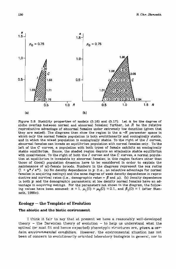
a a1.5 1.5

Po = 0.75

1.0

A1.0

1.30

C

0.5 1.58 0.5

-

Po = 0.75

1.,

~1.06 j,

X.1

3.06

I 1.41 2.23 C

1.01J< 1.66 2.25 ~

11.13 1.81 2.25.2.71\ 2.84I I

130

(a)

0.5 1.0 R

(bl

0.5 1.0

N. Chr. Stenseth.

1.5 R

Figure 5.8 Stability propert.ies of models (5.16) and (5.17). Let. a be t.he degree ofniche overlap bet.ween normal and abnormal females; furt.her, let. R be t.he relat.ivereproduct.ive advant.age of abnormal females under ext.remely low densit.les (given t.hat.t.hey are mat.ed). The diagrams t.hen show t.he region in t.he a -R paramet.er space inwhich only t.he normal female populat.ion is bot.h evolut.ionarily and ecologically st.able,and in which t.he mixed populat.ion is ecologically st.able. To t.he right. of t.he I curves,abnormal females can invade an equilibrium populat.ion wit.h normal females only. To t.heleft of t.he C curves, a populat.ion wit.h bot.h t.ypes of female exhibit.s an ecologicallyst.able equilibrium. Hence, t.he shaded region depict.s an attainable st.able equilibriumwit.h coexist.ence. To t.he right. of bot.h t.he I curves and t.he C curves, a normal popula­t.ion at. equilibrium is invadable by abnormal females; in t.his region fact.ors ot.her t.hant.hose of (local) populat.ion dynamics have t.o be considered in order t.o explain t.hemaint.enance of all-female broods. Numbers in t.he diagrams represent. t.he sex ratios(1 + y* I x*). (a) No densit.y dependence in p (Le., no select.ive advant.age for normalfemales in acquiring mat.ings) and t.he same degree of weak densit.y dependence in repro­duct.ive and survival rat.es (Le., demographic rat.es - (3 and /-1-). (b) Densit.y dependencein bot.h p and t.he demographic paramet.ers; at. low densit.y normal females have an ad­vantage in acquiring matings. For t.he paramet.ers not. shown in t.he diagram, t.he follow­ing values have been assumed: ex =1, /-1-1(0) =j.Iz(O) =0.1, and (31(0) =1 (after St.en­set.h, 1985c).

Ecology - the Template of Evolution

The abiotic and the biotic environment

I think it fair to say that at present we have a reasonably well-developedtheory - the Darwinian theory of evolution - to help us understand what theoptimal (or most fit and hence expected) phenotypic structures are, given a cer­tain environmental condition. However, the environmental situation has notbeen of concern to evolutionarily oriented laboratory biologist.s in general, nor to

DarwiniBn Evotution in Ecosystems

a1.0

Po = 0.5

c

0.5

131

oo 0.5 R

Figure 5.9 The stability properties of models (5.16) and (5.17) in the absence of densitydependence in demographic rates and in p. For a fixed Po' this stability region (see Fig­ure 5.8) remains unchanged as do the sex ratios in various parts of this region, regard­less of the degree of density dependence (as long as this degree is equal in p as well asin (3 and in j.L). However, actual densities increase in the shaded region to infinity as thedegree of density dependence diminishes to zero.

population geneticists in particular. Specifically, this was not a problem for thepioneers in the field, such as Ronald Fisher and J .B.S. Haldane: they considered,in most cases, only one species in an otherwise constant environment - and theyalmost never treated species-species interactions.

As a result, we have at present no convincing theory of ecology. This isunfortunate since, as I have pointed out above, the total environment of a givenspecies consists partly of its abiotic environment and partly of its biotic environ­ment, where the biotic component comprises other coexisting species, each ofwhich plays the same game; they are all evolving as a result of natural selection.The challenges of evolving species are faced with because of a changing abioticenvironment are likely to be of a qualitatively different kind to those of a chang­ing biotic environment (due to evolution of coexisting species). Furthermore,these evolutionary issues will probably be studied using quite different methods.

Following Maynard Smith (1982c), what we need

... is a theory which says something about natural selection, and hence aboutthe environment. Since the major component of the environment of mostspecies - in most cases - consists of other species in the ecosystem, it fol­lows that we need a theory of of ecosystems in which the component speciesare evolving by natural selection.

132 N. Chr. Stenseth

What we need in ecology is something like Weismann's general theory of develop­ment; but such a theory is hard to formulate. The building blocks must, I am con­vinced, be the Darwinian theory of evolution and a theory of ecology; the formerwe have, the latter we do not have. The data for testing such a theory would, I amsure, have to be provided by paleontology and ecology.

A question, two answers, and a possible solution

To demonstrate how difficult is the situation that evolutionary biology is in,it is worthwhile to note that it is now far easier to ask the following question thento answer it: Will evolution cease if we stop all physical disturbances - regular andirregular - of the environment due to factors like seasonal changes and randomlychanging weather conditions? It turns out, indeed, that very competent biologistsmight give quite opposite answers to this question - and that each of them willdefend their position rather strongly. Unfortunately, it is at present rather diffi­cult to say who is right. And that suggests to me that something is wrong, and thatsomething important is missing in current Darwinism. I have no doubt that it is amore solid understanding of ecology and a more synthetic theory of ecology thatare missing.

How, then, can ecology more properly be incorporated into evolutionaryarguments (and into the theory of evolution)? Van Valen (1973) suggested (in thesame paper in which he presented the "Law of Constant Extinction") the RedQueen hypothesis: the Red Queen, you will remember, explained to Alice inWonderland (Carroll, 1871) that

... it takes all the running you can do, to keep in the same place. If you wantto get somewhere else, you must run at least twice as fast as that.

Van Valen's Red Queen view of evolution then asserts that any evolutionary changein any species is experienced by coexisting species as a change of their environ­mental conditions. Hence, a species must evolve as fast as it can in order to con­tinue its existence. If the species does not evolve as fast as it can, it will becomeextinct. An "arms race" (Dawkins and Krebs, 1979) results: this I call the RedQueen type of evolution.

Darwin (1859) had very similar ideas:

the most important of all causes of evolution is one which is almost indepen­dent of ... altered physical conditions, namely, the mutual relation of organ­ism to organism ...

Furthermore, Darwin said:

... if some of these species become modified and improved, others will have tobe improved in a corresponding degree or they will be exterminated.

Van Valen (1973) claimed that his Red Queen hypothesis would explain the "Law ofConstant Extinction", but his argument was, however, not convincing (e.g., May­nard Smith, 1976a; Stenseth, 1979).

Darwinian EvoLution in Ecosystems

A Darwinian Theory of Evolution in Ecosystems

133

Previously, I have reviewed several models for the Red Queen hypothesis(Stenseth, 1979, 1985a) - some developed specifically for it and others appropri­ate for analyzing it - and I do not repeat this discussion herein. However, I doemphasize the potential prospects of the models due to Kerner (1957, 1959) on"the statistical mechanics of population dynamics" even though there are severaldifficulties with this approach (see, e.g., Maynard Smith. 1974; Stenseth. 1979.1985a; Case and Casten. 1979). In addition to the difficulties mentioned in myear­lier writings. there is yet another: the species number in the community ofinteracting organisms should be allowed to vary as a result of speciation. immigra­tion, and extinction. I do not know whether this is at all possible, but some com­petent mathematician should think about it - if advancements are made, theycould benefit evolutionary ecology greatly.

The lag load

Maynard Smith (1976a) specified the Red Queen hypothesis by introducingthe evolutionary la~ load concept. Let L i be the lag load of the i th species in anarea. Further, let Wi = (1/ xi )(dx / dt) = f i (x) be the i th species' current meanfitness [see equation (5.9); also Stenseth, 1983a] and let Wi be the maximal possi­ble fitness of the species in the current environment which it would have if allpossible favorable alleles, whether or not they are yet segre~atin~, are incor­porated. As pointed out by Stenseth and Maynard Smith (1984), Wi / Wi is. in prin­ciple, a measurable quantity; hence, L i is measurable. Using these concepts, Li isdefined as

(5.18)

A community with a fixed number or species

Assume first that a fixed number of species coexist in the community. Let6Li denote the change in unit time of the i th species' lag load. As explained byMaynard Smith (1976a), Li may be expressed as

6Li = 6e L i - OgLi (5.19)

where 0eLi is the change in the i th species' lag load due to (micro-) evolution ofthe S-l coexisting species (Le.. change in its biotic environment) and ogLi is thechange in the i th species' lag load due to its own (micro-) evolutionary approachto its adaptive peak as defined by its current environment.

Let f3 ij measure the increase in the i th species' lag load caused by a unitchange in the jth species' lag load. Then we may rewrite equation (5.19) as

6Li = 'Lf3ij 6g L i - 6g L i (5.20)j

(where, of course, f3 ii = 0). Assuming that 6g Li may be expressed as kiLi (which.in fact, is a generalized form of Fisher's fundamental theorem of natural selection;

134 N. Chr. Stenseth

(5.21)

(5.22)

see Stenseth and Maynard Smith, 1984) and putting L = (11 S) I;Li , we obtaini

dL/dt = (kIS)[I;(Lj 2;{fij) - 2;Lj ] .j i j

As pointed out by Maynard Smith (1976a), model (5.21) only has a stationaryequilibrium point if 2; {f ij == 1 for all j; if I; {fij < 1 for most j , i would decrease

i iand evolution in the community would be in what Maynard Smith called the conver-gent mode; if, however, I; {fij > 1 for most j, i would increase and evolution in

ithe community would be in what Maynard Smith called the divergent mode. Aspointed out by Stenseth (1979), these conclusions do not refer to the globalbehavior of the model since both {f and S are treated as constants - which they,of course, are not. Hence. the conclusion reached by Maynard Smith (1976a), thatthe Red Queen hypothesis seems to be implausible. is not necessarily correct (seeStenseth, 1979; and the next section).

A community with a changing number or species

Stenseth (1979) pointed out that changing the number of species in the sys­tem (as a result of speciation, immigration, and/or extinction) would, in general.change the values of {fij and thus the value of 2;{fij for the various j. In order to

istudy the effects of changing S, Stenseth and Maynard Smith (1984) studied thedynamic behavior of the following system:

- -dL I dt = (a + bL + cS)L

dS I dt = h + (d - e)i + (J - g)S

in which they argued that b < 0, h > 0 and (J - g) < 0, but with a, c, and d - eof uncertain sign. The complete dynamic behavior of model (5.22) is summarized inFigure 5.10 (for details, see Stenseth and Maynard Smith, 1984; and also Stenseth,1985a). As can be seen, both a Red Queen type of continued evolution and a sta­tionary state without any evolutionary changes may occur in a physically stableenvironment: a similar distinction also emerges in the case of some background,low-level physical noise (see Stenseth, 1985a). Stenseth and Maynard Smith (1984)suggest that the Red Queen type of coevolution corresponds to the gradualisticpattern of evolution (see pp 107-108), whereas the stationary state correspondsto the punctualistic pattern of evolution (see above).

Obviously, model (5.22) is too general to be of much help in interpreting thefossil record in any detail. However, it does demonstrate that a reasonableDarwinian model may be formulated which predicts both the gradualistic and thepunctualistic pattern, depending on the values of the parameters. This conclusionis, to my mind, important since it shows that it is not necessarily correct to say,as, for example, Gould (1980, 1982), Stanley (1975, 1979, 1982), and Stanley et at.(1983) do, that the punctualistic pattern of the fossil record cannot be predictedon the basis of Darwinism. Specifically, the analysis carried out by Maynard Smithand myself demonstrates clearly that one cannot draw conclusions regarding

Da;rwinia;n EvoLution in Ecosystems 135

[

d-e<O

[=0 [

d-e>O

t=O

>-------'---""'---s

(a) Red Queen = steady state

[

(d) Exti'netion or Explosion

[

5=0C"'=Oa<O

(b) Stationary (e) Extinction

[ ...L = 0 [ [=0

5=0c<oa>O

""'---=--_L------"'~_S

(c) Stationary or Extinction (f) Red Queen = steady state

Figure 5.10 The dynamic behavior of model (5.22) for various combinations of parame­ters. As can be seen, both the gradual Red Queen type of evolution and the stasis-plus­punctuation type may result. The dynamics of the~volutionarysystem for various valuesof a., C, and d - e are shown. Notice that the dL / dt isocline in (e) does not intersectth~ dS / dt isocline since the latter approaches an asymptote far to the left of thed.L / dt isocline.

mechanisms on the basis of observed patterns (see Maynard Smith, 1982c, for arelevant discussion).

Several other conclusions can be drawn from this analysis: first, the RedQueen hypothesis is plausible: as explained above, depending on the parameters ofthe system the Red Queen mechanism may lead to either a Red Queen type of evo­lution or to stagnation. Second, the "Law of Constant Extinction" follows from theRed Queen hypothesis. Several other applications are discussed by Stenseth(1985a). Most important in this context is the suggestion that if evolution is of theRed Queen type and continues for ever even in a physically stable environment,increasingly more complex forms (defined in some proper way) tend to evolve.

136 N. Chr. Stenseth

Two more general conclusions about evolution may be drawn from model (5.22):

(1) I have elsewhere (stenseth, 1985b) argued on the basis of this model that thetropics may properly be considered the cradle of most of the world's biota;the tropics are. however, a bad museum since the rate of extinction is highbecause of the higher species diversity.

(2) I have further suggested (Stenseth, 1985d) on the basis of this model thatevolutionary novelties are more likely to arise in environmentally unstableregions than in environmentally stable regions. Essentially, this is so becausethe pattern depicted in Figure 5.10 (b) is more likely to occur in physicallyunstable regions, whereas the pattern depicted in Figure 5.10 (a) is morelikely to occur in physically more stable regions. Some observations suggestthe validity of this prediction (Jablonski et eLL., 1983; Hickey et eLL., 1983;Zinmeister and Feldman, 1984; see also Stenseth, 1985d).

Finally, it seems plausible that this kind of Red Queen model for coevolutionin ecosystems should be able to explain observations that suggest convergent evo­lution at the community level (e.g., Orians and Paine, 1983). Much work remains tobe done in this area, though.

Environs - an alternative approach

Based on the system ecology approach (e.g., Odum, 1969, 1971), Patten andhis co-workers have taken another route (e.g., Patten, 1975, 1978, 1981, 1982,1983, 1985; Patten and Auble, 1980, 1981; Patten and Odum, 1981; Patten et eLL.,1976); Wilson's (1980) approach is along similar lines.

As in the case of the Red Queen approach (e.g., Maynard Smith. 1976a; Sten­seth and Maynard Smith, 1984), evolution is, as far as I understand, assumed toproceed by natural selection of individual organisms due to both direct andindirect effects (generating the selective pressure) of the environment. Also, as inthe model of Stenseth and Maynard Smith (1984), the ecological niche (e.g., Grin­nell, 1917, 1928; Elton, 1927; Hutchinson, 1957; Pianka, 1978; Roughgarden, 1979)is assumed to represent the point of direct contact between organisms and theirenvironment (both its abiotic and biotic parts). Patten and his co-workers (e.g.,Patten, 1981, 1983; Patten and Auble, 1980, 1981) suggest, however, a new theoret­ical concept, the environ, which is the unit of organism-environment coevolution.At least to me, this appro!'-ch seems exceedingly complex, described in a highlydeveloped system-theory jargon. However, I have a very strong feeling that itmight be important in helping us out of some of the difficulties we are faced within evolutionary theory today. This approach. linked with Van Valen's (1973) RedQueen view of evolution might provide an important advancement and should beat tempted by someone better qualified than 1.

But to hypothesize that evolution favors linearity at the ecosystem level, orthat undesirable effects of nonlinearity at the ecosystem level are selectedagainst, as Patten (1975, 1983) suggests, is - I believe - a wrong track: such aselection seems only to be possible if ecosystems, or the like, are the unit of evo­lution. And as demonstrated by Maynard Smith (1976b), group selection of thistype is likely to be far less efficient than evolution at the individual level - or atsome lower level of organization. See Stenseth (1984c) for a general discussion ofecosystem evolution.

Darwinian Evolution in Ecosystems

What kind or models do we need?

137

Previously (Stenseth, 1983a, 1985a: see also 1984c) I have discussed thekinds of mathematical models we would need in order to understand the operationof natural selection in a dynamic community which changes with respect to bothnumber and phenotypic properties of the coexisting species. This is, to my mind,the most important technical problem to solve before we can develop improvedmodels for evolution in ecosystems.

Consider a model of the kind

(5.23)

where %1. is the density of the ith species (i = 1,2, ...• S, where S is the totalnumber of coexisting species), and 11. is the specific growth rate of the i thspecies [see equation (5.9)]. For a fixed number of species, S, and nonchanging 11.'

model (5.23) is a standard population dynamics model referring to ecological time(sensu Stenseth and Maynard Smith, 1984); here %1. are the only variables. As dis­cussed above, the Ii-functions, however, change as a result of microevoluionoccurring on what might be called a population genetic time scale (sensu Stensethand Maynard Smith, 1984; see also Lawlor and Maynard Smith, 1978). For a commun­ity with a fixed number of species, 11. may reach an ESS or a CSS state (Schafferand Rosenzweig, 1978; see also Roughgarden, 1979). Several theorists contend thatit is sufficient to study few-species assemblages (e.g., Beddington and Lawton,1978). Models of many-species communities - maybe with more tightly packed sub­systems - are, however, important to analyze since we know that diffuse competi­tion does occur fairly frequently (see, e.g., Pianka, 1978, 1980).

We have mathematical techniques available for analyzing both the populationdynamic and microevolutionary changes. However, as pointed out in the previoussubsection, S is also a dynamic variable changing on a fairly slow time scale as aresult of speciation and extinction (see Stenseth and Maynard Smith, 1984). As faras I know, there is no standard analytical technique available for analyzing model(5.23) with S as a dynamic variable (but see the section on environs above)*. Thedevelopment of such techniques would, I am sure, greatly benefit evolutionary biol­ogy.

I am at present unable to recommend what sorts of mathematics should beused for analyzing the problems discussed in this chapter. However, one thing isimportant to remember whan choosing which mathematics to use in various fieldsof the natural sciences: living material is, by definition, characterized by unitshaving the properties of reproduction, inheritance, and variation (see p 112).Nonliving material is everything else. As is apparent, I have in this chapter on liv­ing material been using mathematics primarily developed for the nonliving world.That might be a serious shortcoming of all the studies I have reviewed.

I am afraid I have been very vague in my recommendations; I wish I could bemore precise and specific.

·Several good discussions of the modellng of such evolving ecosystems exist, however (e.g.,Beddlngton and Lawton, 1978; Roughgarden, 1979); see also the Interesting and relevant discus­sion presented by Johnson (1981).

138

A Synopsis of Darwinism

N. Ch.r. Stenseth.

The basic premises in the Darwinian theory of evolution (Le., Darwinism) arereprod.uction, inheritance, and variation. If a population of individuals ischaracterized by these properties, evolution may occur as a result of naturalselection; if the environmental situation changes, evolution occurs, in general, as aresult of natural selection adapting the organism to the new environmental condi­tions. In this way the population evolves closer to its adaptive peak. Where thisadaptive peak is located (Le., which phenotype corresponds to the adaptive peak)is determined by the coexisting species (i.e., the biotic properties of the environ­ment) as well as by the abiotic properties of the environment.

These microevolutionary changes brought about by natural selection due to(phenotypic) fitness differences are reflected in genotypic changes (Le., genefrequency changes) in the population. Notice, however, that many genotypicchanges may occur without any corresponding phenotypic change: this we callnon-Darwinian evolution (Kimura, 1983).

Referring to Figure 5.11. we may then say that the shape of the fitness curve(and in particular the location of the adaptive peak along the phenotype axis) isdetermined by the environment (both biotic and abiotic); since we presently haveonly vague ideas about ecology, we have only vague ideas about how this fitnesscurve is determined. The location of any individual along the phenotype axis isdetermined by the d.evelopmental processes; even though we have very vagueideas at present about developmental biology, we know that for any particulargenotype there is, in a particular environment, a particular phenotype thatdevelops. This process is a many-to-one mapping. Which genotype is selected is

", -----------2: "2 ------------enenQlc:

.-=u..

c, C c2Phenotypic character

Figure 5.11 A synopsis of Darwinian evolution in ecosystems. The phenotype c is the op­timal one under current environmental conditions (see text for further discussion). Thepositions of the fitness curve and c are determined by the environment. The positions ofthe two depicted organisms' phenotypes (c 1 and c2) are determined by their genotypesand environments. Which one is favored in the process of evolution is determined by theDarwinian process of natural selection (comparing )0.1 and 71.2),

Darwinian EvoLution in Ecosystems 139

then determined by the fitness (or some analogous property) of this phenotypecompared with other phenotypes' fitnesses. According to the theory of naturalselection. the one with the highest fitness is selected.

Since we do not understand development (and, in particular. since we do nothave a theory for development) we cannot predict the course of evolution. Buteven without such a theory for development, we can predict that evolution occursif the fitness curve changes. But without a theory for ecology we are unable tosay what is needed to change the fitness curve.

After more than one hundred years of research into the Darwinian theory ofnatural selection, we have a fairly good understanding of how natural selectionoperates for a given selective pressure. However, this is of little use when tryingto predict the long-term patterns of the fossil record, since we do not understandhow the fitness curve changes as a result of evolution in coexisting species. Thatis, we do not understand what generates the selective pressure. For that reason,study ecology! And even more, try to develop a general theory for ecology.

Then, having such a theory for ecology, we might be able to solve several ofthe current controversies in biology today and assist the solution of practicalproblems like pest control and resource management (see. e.g., Stenseth, 1983a,1984c).

Today there is certainly no indication that Darwinism ought to be rejected.The only solid experimental threats to the Darwinian view are the observations ofnonchromosomal inheritance (such as. e.g., the phenomena of cortical inheritancein ciliates; e.g., Steel, 1979; see also Brooks, 1983). Darwinists should, as MaynardSmith (1983) emphasized, not be allowed to forget these observations - doing thatwould be to reject critical evidence against one's view. However, the very reasonfor not rejecting the Darwinian view in spite of such observations is that theoverwhelming majority of inherited differences between organisms are caused bychromosomal genes - hence the Weismannian assumption holds true in the majorityof cases.

Contrary to some writers' views (Gould, 1980, 1982; Stanley, 1979; Stanley etat., 1983), the pattern of stasis-pIus-punctuation seen in the fossil record [Figure5.3(a)] certainly constitutes no reason to reject the Darwinian approach (seeabove): at best, such observations only suggest that we have to refine existingtheory (see Maynard Smith, 1982c, for a relevant discussion).

Above all, we have to bring ecology (back) into evolutionary theory - orrather, we have to study the organism-environment as a synergistic whole. Ecol­ogy and the Darwinian evolutionary theory should no longer

... remain ... separate disciplines, travelling separate paths while politelynodding at each other as they pass. (Lewonlln, 1979).

I hope that some of the studies reviewed in this chapter may help to bringecology and evolution into a closer, truly mutual relationship. Much remains to bedone - but the seeds for a unified theory of evolutionary biology are there. Mostof all, we must weed our flower-bed. Unfortunately, this is rather hard when we donot know for sure which seedlings are weeds and which seedlings are the flowerswe want to grow. I only wish I knew how to tell them apart.

140

Acknowledgements

N. Chr. Stenseth

My work on evolutionary biology has been generously funded by theNorwegian (NAVF) and Swedish (NFR) science foundations, the Nansen Foundation,and the Nordic Council for Ecology. I am grateful to the organizers of the Abiskomeeting (Anders Karlqvist, Pehr Sfillstrom, and Uno Svedin) for inviting me topresent my thoughts on the subject - hence forcing me to think through theentire field once more. Discussions with Stig Omholt were essential for summariz­ing my ideas into one figure, Figure 5.11. Tove Valmot is thanked for perfect secre­tarial work in finishing the manuscript under rather exceptional conditions:without her help, there would have been no chapter.

References

Alberch, P. (1980) Ontogenesis and morphological diversification. Am. Zool. 20: 653-67.Allen, P.M. (1976) Evolution, population dynamics and stability. Proc. Natl. Acad. Sci.

(USA) 73: 665-8.Arnold, V.I. (1973) Ordinary Differential Equations (Cambridge, MA: MIT Press).von Baer, K.E. (1828) Uber Entwicklungsgeschichte der 1'iere. Beobeachtung und

Rejtezion (Konigsberg: Borntrager).Barlow, G.W. et al. (1984) Open peer commentary - 18 separate replies to Maynard

Smith's (1984) article. Behav. Brain Sci. 7: 101-17.Beddington, J.R., and Lawton, J.H. (1978) On the structure and behaviour of ecosystems.

Colloque Ct5, suppl. no 8; 39: 39-43.Bonner, J.T. (Ed) (1982) Evolution and Development (New York: Springer Verlag).Bowler, P.J. (1975) The changing meaning of 'evolution'. J. Hist. Ideas 36: 95-114.Brooks, D.R. (1983) What's going on in evolution? A brief guide to some new ideas in evo-

lutionary theory. Can. J. Zool. 61: 2637-45.Bull, J.J. (1983) Evolution of Se:r: Determining Mechanisms (Menlo Park. CA:

Benjamin/Cummings Publ. Co.).Calow, P. (1983) Evolutionary Principles (Glasgow: Blackie).Carroll, L. (1871) Through the Looking-Glass and what Alice found there (Reprinted

in 'Alice in Wonderland', W.W. Norton Co. Inc. NY, 1971).Case, T.J. (1982) Coevolution in resource-limited competition communities. Theor. pop.

Biol. 21: 69-91.Case, T.J. and Casten, R.G. (1979) Global stability and multiple domains of attraction in

ecological systems. Am. Nat. 113: 705-14.Case, T.J. and Sidel, R. (1983) Pattern and change in the structure of model and natural

communities. Evolution 37: 832-49.Charlesworth, B. (1980) Evolution in Age Structured Populations (Cambridge, UK:

Cambridge University Press).Charlesworth, B., Lande, R., and Slatkin, M. (1982) A neo-Darwinian commentary on

macroevolution. Evolution 36: 474-98.Charnov, E.L. (1982) Parent-offspring conflict over reproductive effort. Am. Nat. 119:

736-7.Colbert, E.H. (1969) Evolution of the Vertebrates, 2nd edn (New York: Wiley).Crick, F.H.C. (1958) The biological replication of macromolecules. S'ymp. Soc. E:r:p. Biol.

12: 138-63.Crick. F.H.C. (1970) Central Dogma of molecular biology. Nature 227: 561-3.Crick, F.H.C. (1973) Project K: The complete solution of E. coli. Perspectives in Biol.

and Medicine 17: 67-70.Darwin. C. (1859) On the Origin of Species by Means of Natural Selection. or the

Preservation ofFavoured Races in the Struggle for Life (London: John Murray).

Darw1.n1.anEtJoLut1.on in EcoS1Jstems 141

Dawkins, R. (1976) The Selfish Gene (Oxford: Oxford University Press).Dawkins, R. (1982) The Extended Phenotype (San Francisco: Freeman).Dawkins, R. and Krebs, J.R. (1979) Arms races between and within species. Proc. Roy.

Soc. Lond. B 205: 489-511.Diamond, J.M. (1969) Avifaunal equilibria and species turnover rates on the Channel

Island of California. Proc. Natl. Acad. Sci. (USA) 64: 57-63.Dobzhansky, T., Ayala, F.J., Stebbins, G.L., and Valentine, J.W. (1977) Evolution (San

Francisco: Freeman).Eldredge, N. and Gould, S.J. (1972) Punctuated equilibria: an alternative to phyletic

gradualism, in T.J.M. Schopf (Ed) Models in Paleobiology (San Francisco: Freeman)pp 82-115.

Elton, C.S. (1927) Animal Ecology (London: Sidgewick & Jackson).Elton, C.S. (1958) The Ecology of Invasions by Animals and Plants (London: Methuen).Fisher, R.A. (1930) The Genetical Theory of Natural Selection (Oxford: Clarendon

Press).Fredga, K. (1983) Aberrant sex chromosome mechanisms in mammals. Evolutionary

aspects. Differentiation 23 (Suppl.): S20-S30.Fredga, K., Gropp, A., Winking, H., and Frank, F. (1976) Fertile XX- and XY-type females

in the wood lemming (Myopus schisticolor). Nature 261: 225-7.Fredga, K., Gropp, A., Winking, R., and Frank, F. (1977) A hypothesis explaining the

exceptional sex ratio in the wood lemming (Myopus schisticolor). Hereditas 85:101-4.

Futuyma, D.J. (1979) Evolutionary Biology (Sunderland, MA: Sinauer Assoc.).Goldschmidt, R.B. (1940) The Material Basis of Evolution (New Haven, CT: Yale Univer­

sity Press).Gould, S.J. (1980) Is a new and general theory of evolution emerging? Paleobiology 6:

119-30.Gould, S.J. (1981) Paleontology plus ecology as paleobiology, in R.M. May (Ed) Theoreti­

cal Ecology; Principles and Applications, 2nd edn (Sunderland, MA: SinauerAssoc.) pp 295-317.

Gould, S.J. (1982) Darwinism and the expansion of evolutionary theory. Science 216:380-7.

Gould, S.J. (1983) Punctuated equilibria in the fossil record (a reply). Science 219:439-40.

Gould, S.J. and Eldredge, N. (1977) Punctuated equilibria: the tempo and mode of evolu­tion reconsidered. Paleobiology 3: 115-51.

Grinnell, J. (1917) The niche relationships of California thrasher. Ank 21: 354-82.Grinnell, J. (1928) The presence and absence of animals. Univ. Calif. Chronicle 30:

429-50.Haeckel, E. (1866) Generelle Morphologie der Organismen, 2 vols (Berlin: G. Reimer).Haldane, J.B.S. (1932) The Causes ofEvolution (London: Longmans, Green & Co.).Hallam, A.A. (1976) The Red Queen dethroned. Nature 259: 12-3.Hamilton, W.D. (1964a) The genetical evolution of social behaviour 1. J. theor. Biol. 7:

1-16.Hamilton, W.D. (1964b) The genetical evolution of social behaviour II. J. theor. Biol. 7:

17-52.Hamilton, W.D. (1967) Extraordinary sex ratios. Science 156: 477-88.Heuch, I. (1978) Maintenance of butterfly populations with all-female broods under

recurrent extinction and recolonization. J. theor. Biol. 75: 115-22.Hickey, L.J., West, R.M., Dawson, M.R., and Choi, D.K. (1983) Arclic terrestrial biota:

paleomagnetic evidence of age disparity with mid-northern latitudes during thelate coclaceous and early tertiary. Science 221: 1153-6.

Hutchinson, G.E. (1957) A Treatise on Limnology; Vol. 1, Geography, Physics andChemistry (New York: Wiley).

Jablonski, D., Sepkoski, J.J., Bottjer, D.J., ar,d Sheehan, P.M. (1983) Onshore-offshorepatterns in the evolution of Phanerozoic shelf communities. Science 222: 1123-5.

142 N. Ch.r. Stenseth.

Johannsen, W. (1909) ET.emente der e:z:aJc:ten Erblichkeitslehre (Jena: Guslav Fisher).Johnson, L. (1981) The thermodynamic origin of ecosystems. Can. J. Fish. Aquat. Sci.

38: 571-80.Kalela, O. and Oksala, T. (1966) Sex ratio in the wood lemming, Myopus schisticolor

(Lilljeb.) in nature and captivity. Ann. Univ. Turkuensis, Ser. All, 37: 1-24.Kerner, E.H. (1957) A slatistical mechanistics of interacting biological species. Bull.

Math. Biophysics 19: 121-46.Kerner, E.H. (1959) Further considerations of the slatistical mechanistics of biological

associations. Bull. Math. Biophysics 21: 217-35.Kimura, M. (1983) The Neutral Theory of Molecular Evolution (Cambridge, UK: Cam­

bridge University Press).Kostitzin, V.A. (1938) l!:quations dlff~rentielles g~n~rales du probl~me de s~lection

naturelle. Comptes rendus 203: 156-7.Lamarck, J.B. (1809) Philosophie Zoologique (Paris: Librairie Schleicher Fnkes).Lander, G.V. (1982) Historical biology and the problem of design. J. theor. Biol. 97:

57-67.Lawlor, L.R. and Maynard Smith, J. (1976) The coevolution and slability of competing

species. Am. Nat. 110: 79-99.Le6n, J.A. (1976) Life histories as adaptive strategies. J. theor. Biol. 60: 301-35.Levins, R. (1968) Evolution in Changing Environments (Princeton, NJ: Princeton

University Press).Lewontin, R. (1974) The Genetical Basis of Evolutionary Change (New York: Columbia

University Press).Lewontin, R. (1979) Fitness, survival and optimality, in D.J. Horn, G.R. Stairs, and R.D.

Mitchell (Eds) Analysis of Ecological Systems. (Columbia: Ohio Slate UniversityPress) pp 3-21.

Lundberg, S. and Stenseth, N.C. (1985) Coevolution of competing species: convergent anddivergent evolution and crossover in character displacement. Theor. pop. Biol. (inpress).

MacArthur, R.M. (1972) Geographical Ecology: Patterns in the Distribution of .species(New York: Harper & Row).

MacArthur, R.M. and Levins, R. (1967) The limiting similarity, and character displace­ment in a patchy environment. Proc. Natl. Acad. Sci. 51: 1207-10.

MacArthur, R.M. and Wilson, E.O. (1967) The Theory of Island Biogeography (Princeton,NJ: Princeton University Press).

Maynard Smith, J. (1960) Continuous, quantized and modal variation. Proc. Roy. Soc.,Lond. B 152: 397-409.

Maynard Smith, J. (1969) The status of nee-Darwinism, in C.H. Waddington (Ed) Towardsa Theoretical Biology, Vol. Z, Sketches (Edinburgh: Edinburgh University Press) pp82-9.

Maynard Smith, J. (1972) On Evolution (Edinburgh: Edinburgh University Press).Maynard Smith, J. (1974) Models in Ecology (Cambridge, UK: Cambridge University

Press).Maynard Smith, J. (1975) The Theory of Evolution, 3rd edn (Harmondsworth: Penguin

Books).Maynard Smith, J. (1976a) A comment on the Red Queen. Am. Nat. 110: 331-8.Maynard Smith, J. (1976b) Group selection. Quart. Rev. Biol. 51: 227-83.Maynard Smith, J. (1978a) Optimization theory in evolution. Ann. Rev. Ecol. Syst, 9:

31-56.Maynard Smith, J. (1978b) The Evolution of Se:z: (Cambridge, UK: Cambridge University

Press).Maynard Smith, J. (1982a) Introduction, in J. Maynard Smith (Ed) Evolution Now (Lon­

don: MacMillan) pp 1-6.Maynard Smith, J. (1982b) Evolution and the Theory of Games (Cambridge, UK: Cam­

bridge University Press.).Maynard Smith, J. (1982c) Evolution - sudden or gradual? (Introduction to ch. 5) in J.

Maynard Smith (Ed) Evolution Now (London: Macmillan) pp 125-8.

Darwinian EvoLution in Ecosystems 143

Maynard Smith, J. (1983) Evolution and development, in B.C. Goodwin, N. Holder, and C.C.Wylie (Eds) Development and Evolution (Cambridge, UK: Cambridge UniversityPress) pp 33-46.

Maynard Smith, J. (1984) Game theory and the evolution of behaviour. Behav. BrainSci. 7: 94-101 (see reply to "Open Peer Commentary" pp. 117-125).

Maynard Smith, J. and Price, G.R. (1973) The logic of animal conflict. Nature 246: 15-8.Maynard Smith, J. and Sondhi, K.C. (1960) The genetics of pattern. Genetics 45:

1039-50.Maynard Smith, J. and Sondhi, K.C. (1961) The arrangement of bristles in Drosophila. J.

Embryol. exp. Morph. 9: 661-72.Maynard Smith, J. and Stenseth, N.C. (1978) On the evolutionary stability of the female­

biased sex ratio in the wood lemming (Myopus schisticolor): the effect of inbreed­ing. Heredity 41: 205-14.

Mayr, E. (1961) Cause and effect in biology. Science 134: 1501-6.Monod, J. (1971) Chance and Necessity: an Essay on the Natural Philosophy of

Modern Biology (New York: Knopfer).Odum, E.P. (1969) The strategy of ecosystem development. Science 164: 262-70.Odum, E.P. (1971) fundamentals ofEcology , 3rd edn (Philadelphia: Saunders).Orians, G.H. and Paine, R.T. (1983) Convergent evolution at the community level, in D.J.

Futuyma and M. Slatkin (Eds) Coevolution (Sunderland, MA: Sinauer Assoc.) pp431-59.

Oster, G. and Alberch, P. (1982) Evolution and bifurcation of developmental programs.Evolution 36: 444-59.

Oster, G., Odell, G., and Alberch, P. (1980) Mechanics, morphogenesis and evolution.Lect. Math. Li,fe Sci. 13: 165-255.

Patten, B.C. (1975) Ecosystem linearization: an evolutionary design problem. Am. Nat.109: 529-39.

Patten, B.C. (1978) Systems approach to the concept of environment. Ohio J. Sci. 78:206-22.

Patten, B.C. (1981) Environs: the superniches of ecosystems. Am. Zool. 21: 845-52.Patten, B.C. (1982) Environs: relativistic elementary particles for ecology. Am. Nat. 119:

179-219.Patten, B.C. (1983) Linearity enigmas in ecology. Ecol. Modelling 18: 155-70.Patten, B.C. (1985) Further developments toward a theory of the quantitative importance

of indirect effects in ecosystems, in B.C. Patten (Ed) System Analysis and Simu­lation in Ecology, vol. 00 (in press).

Patten, B.C. and Auble, G.T.(1980) Systems approach to the concept of niche. Synthese43: 155-81.

Patten, B.C. and Auble, G.T. (1981) Systems theory of the ecological niche. Am. Nat. 118:345-69.

Patten, B.C. and Odum, E.P. (1981) The cybernetic nature of ecosystems. Am. Nat. 118:886-95.

Patten, B.C., Bosserman, R.W., Finn, J.T., and Cale, W.G. (1976) Propagation of cause inecosystems, in B.C. Patten (Ed) System Analysis and Simulation in Ecology. Vol.4 (New York: Academic Press) pp 457-579.

Patterson, C. (1983) How does phylogeny differ from ontogeny? in B.C. Goodwin, N.Holder, and C.C. Wylie (Eds) Development and Evolution (Cambridge, UK: Cam­bridge University Press) pp 1-32.

Pianka, E.R. (1978) Evolutionary Ecology (New York: Harper & Row).Pianka, E.R. (1980) Guild structure in desert lizards. Dikos 35: 194-201.Reed, J. and Stenseth, N.C. (1984) On evolutionary stable strategies. J. theor. Biol. 108:

491-508.Roughgarden, J. (1974) Species packing and the competition function with illustrations

from coral reef fish. Theor. pop. Biol. 5: 163-86.Roughgarden, J. (1979) Theory of Population Genetics and Evolutionary Ecology: An

Introduction (New York: Macmillan).

144 N. Ch.r. Stenseth.

Roughgarden, J. (1983a) The theory of coevolution, in D.J. Futuyma and M. Slatkin (Eds)Coevolution (Sunderland, MA: Sinauer Assoc.) pp 33-64.

Roughgarden, J. (1983b) Coevolution between competitors, in D.J. Futuyma and M. Slatkin(Eds) Coevolution (Sunderland, MA: Sinauer Assoc.) pp 383-403.

Roughgarden, J., Herckel, D., and Fuentes, E.R. (1983) Coevolutionary theory and thebiogeography and community structure of Anolis, in R. Huey, E.R. Pianka, and T.Schoener (Eds) LizCLrd Ecology: Studies of CL Model OrgCLnism (Cambridge, MA:Harvard University Press) pp 371-410.

Schaffer, W.M. (1977) Evolution, population dynamics, and stablllty. Theor. pop. Biol.11: 326-9.

Schaffer, W.M. and Rosenzweig, M.L. (1978) Homage to the Red Queen. 1. Coevolution ofpredators and their victims. Theor. pop. Biol. 14: 135-57.

Schuster, P. and Sigmund, K. (1983) Replicator dynamics. J. theor. Biol. 100: 533-8.Schopf, T.J .M. (1982) A critical assessment of punctuated equilibria. 1. Duration of taxa.

Evolution 36: 1144-57.Schopf, T.J.M. and Hoffman, A. (1983) Punctuated equilibria in the fossil record. Science

219: 438-9.Sharpe, F.R. and Lotka, A.J. (1911) A problem in age distribution. Phil. MCLg. 21: 435-8.Sigmund, K. (1985) A survey of replicator equations (this volume, Chapter 4).Simpson, G.G. (1953) The MCLjor FeCLtures of Evolution (Columbia: Columbia University

Press).Slatkin, M. and Maynard Smith, J. (1979) Models of coevolution. Qu,CLrt. Rev. Biol. 54:

233-63.Sondhi, K.C. (1962) The evolution of pattern. Evolution. 16: 186-91.Stanley, S.M. (1975) A theory of evolution above the species level. Proc. NCLtl. ACCLd. Sci

(USA) 72: 646-50.Stanley, S.M. (1979) MCLcroevolution: Fb.ttern CLnd Process (San Francisco: Freeman).Stanley, S.M. (1982) Macroevolution and the fossil record. Evolution 36: 460-73.Stanley, S.M., van Valkenburgh, B., and Steneck, R.S. (1983) Coevolution and the fossil

record, in D.J. Futuyma and M. Slatkin (Eds) Coevolution (Sunderland, MA: SinauerAssoc.) pp 328-49.

Stebbins, G.L. and Ayala, F.J. (1981) Is a new evolutionary synthesis necessary? Science213: 967-71.

Steel, E.J. (1979) SomCLtic Selection CLnd AdCLptive Evolution (Toronto: Williams-WallaceProd. Intern).

Stenseth, N.C. (1979) Where have all the species gone? On the nature of extinction andthe Red Queen Hypothesis. Oikos 33: 196-227.

Stenseth, N.C. (1983a) A coevolutionary theory for communities and food web configura­tions. Oikos 41: 487-95.

Stenseth. N.C. (19B3b) Causes and consequences of dispersal in small mammals, in 1.R.Swingland and P.J. Greenwood (Eds) The Ecology of AnimCLl Movement (Oxford:Oxford University Press) pp 63-101.

Stenseth. N.C. (19B4a) Testing evolutionary predictions: a reply to Bleken and Ugland.Oikos 43: 126-8.

Stenseth, N.C. (1984b) Fitness, population growth rate and evolution in plant-grazer sys­tems: a reply to Nur. Oikos 42: 414-5.

Stenseth, N.C. (1984c) Why mathematical models in evolutionary ecology?, in J.H. Cooleyand F.B. Golley (Eds) Trends in EcologicCLl ReseCLrch for the W8Ds (New York: Ple­num Press) pp 239-87.

Stenseth, N.C. (19B5a) Darwinian evolution in ecosystems - the Red Queen view, in P.J.Greenwood, M. Slatkin, and P. Harvey (Eds) Evolution (Cambridge, UK: CambridgeUniversity Press) (in press).

Stenseth, N.C. (1985b) The tropics: cradle or museum? Oikos (in press).Stenseth, N.C. (1985c) A new hypothesis for explaining the maintenance of the all-female

broods in the African butterfly AcrCLeCL encedon (in review).Stenseth, N.C. (1985d) Origin of species in physically stressed environments (in review).

Darwinian EvoLution in Eco:rystems 145

Stenseth, N.C. and Kirkendall, L.R. (1985) On the ecological and evolutionary stability ofpseudogamy; the effect of niche-overlap between sexual and asexual females (inreview).

Stenseth, N.C. and Maynard Smith, J. (1984) Coevolution in ecosystems: Red Queen evolu­tion or stasis? Evolution 38: 870-80.

Stenseth, N.C., Kirkendall, L.R., and Moran, N. (1985) On the evolution of pseudogamy.Evolution (in press).

Thorn, R. (1975) structural Stability and Morphogenesis: An Outline oJ a GeneralTheory oJ Models (Reading, MA: W.A. Benjamin).

Thorsrud, fiT. and Stenseth, N.C. (1985) On the evolutionary stability of the female biasedsex ratio in the wood lemming (Myopus schisticolor) and the collared lemming(Dicrostony:z: groenlandicus): the effect of dispersal in a patchy environment(manuscript for publication).

Turing, A.M. (1952) The chemical basis for morphogenesis. Phil. Trans. Roy. Soc. Ser. B237: 37-72.

Tyler, M.J. (1983) Evolution of gastric brooding, Ch 10 in M.J. Tyler (Ed) The GastricBrooding Frog (London: Croom Helm).

Van Valen, L. (1973) A new evolutionary law. Evol. Theory 1: 1-30.Van Valen, L. (1976) The Red Queen lives. Nature 260: 575.Van Valen, L. (1977) The Red Queen. Am. Nat. 111: 809-10.Weismann, A. (1886) Essays upon Heredity and Kindred Biological Problems (Oxford:

Clarendon Press).Weismann, A. (1893) The Germ-Plasma: A Theory oJ Heredity (Oxford: Clarendon Press).Whittaker, R.H. (1969) Evolution of diversity in plant communities. Brookhaven Symp.

Biol. 22: 178-96.Williamson, P.G. (1981a) Paleontological documentation of speciation in Cenozoic mol­

luscs from Turkana Basin. Nature 293: 437-43.Williamson, P.G. (1981b) Morphological stasis and developmental constraints: real prob­

lems for neo-Darwinism. Nature 294: 214-5.Wilson, D.S. (1980) The Natural Selection oJ Populations and Communities (Menlo

Park, CA.: Benjamin/Cummings).Wolpert, L. (1969) Positional information and the spatial pattern of cellular differentia­

tion. J. theor. Biol. 25: 1-47.Wolpert, L. (1983) Constancy and change in the development and evolution of pattern, in

B.C. Goodwin, N. Holder, and C.C. Wylie (Eds) Development and Evolution (Cam­bridge, UK: Cambridge University Press) pp 47-58.

Zinmeister, W.J. and Feldman, R.M. (1984) Cenozoic high latitude heterogeneity of south­ern hemisphere marine fauna. Science 224: 281-3.

CHAPTER 6

On System Complexity: Identification,Measurement, and Management

John L. Casti

Complexity and Simplicityt

I have yet to see any problem, however complicated, which. whenyou looked at it the right way, did not become still more complicated.

Poul Anderson

The notion of system complexity is much like St. Augustine's description oftime: "What then is time [complexity]? If no one asks me, I know; if I wish toexplain it to one that asks, I know not." There seem to be fairly well-developed,intuitive ideas about what constitutes a complex system, but attempts to axioma­tize and formalize this sense of the complex all leave a vague, uneasy feeling ofbasic incompleteness, and a sense of failure to grasp important aspects of theessential nature of the problem. In this chapter we examine some of the rootcauses of these failures and outline a framework for the consideration of complex­ity that provides a starting point for the development of operational proceduresin the identification, characterization, and management of complex processes. Inthe process of developing this framework for speculation, it is necessary to con­sider a variety of system-theoretic concepts closely allied to the notion of com­plexity: hierarchies, adaptation, bifurcation, self-organization, and reductionism,to name but a few. The picture that emerges is that of complexity as a latent orimplicate property of a system, a property made explicit only through theinteraction of the given system with another. Just as in baseball where somepitches are balls and some are strikes, but "they ain't nothin'" until the umpirecalls them, complexity cannot be thought of as an intrinsic property of an isolated(closed) system; it is only made manifest by the interaction of the system withanother, usually in the process of measurement and/or control. In this sense, it is

tHotes and references relevant to each secl10n are given at the end of the chapter.

On System Comptez'l.ty 147

probably more meaningful to consider complexity more as a property of the inter­action than of the system, although it is clearly associated with both. The explora­tion and exploitation of this observation provides the starting point for an emer­gent theory of complex processes.

Before embarking upon a detailed consideration of complexity in natural andhuman phenomena, it is useful to consider for a moment why a deeper understand­ing of complexity, per se, is of either theoretical or practical importance. Thebasic reason is the seemingly inherent human need to simplify in order to under­stand and direct (control). Since most understanding and virtually all control isbased upon a model (mental, mathematical, physical, or otherwise) of the systemunder study, the simplification imperative translates into a desire to obtain anequivalent, but reduced, representation of the original model of the system. Thismay involve omitting some of the original variables, aggregating others, ignoringweak couplings, regarding slowly changing variables as constants, and a variety ofother subterfuges. All of these simplification techniques are aimed at reducing thedegrees of freedom that the system has at its disposal to interact with its environ­ment. A theory of system complexity would give us knowledge as to the limitationsof the reduction process. For example, it is well known that the three-body prob­lem of celestial mechanics cannot be resolved in analytic terms; however, the two­body problem is completely solvable, but a sequence of two-body problems cannotbe combined to solve the three-body problem. Thus, the complexity of the three­body problem is intrinsically greater than any sequence of two-body problems andthere is an irretrievable loss of information in passing to such a reducedrepresentation. A useful theory of system complexity would provide conditionsunder which such a decomposition would work and perhaps even suggest novel,nonphysical, simpler representations that would be valid when the "natural" sim­plifications fail.

What are the distinguishing structural and behavioral characteristics ofthose systems we intuitively think of as being complex? Perhaps the easiest wayto approach this question is to consider its converse: what features do we associ­ate with simple systems? Some of the most evident properties of simple systemsare:

Predictable behavior. There are no surprises: si.mple systems exhibit abehavior pattern that is easy to deduce from knowledge of the externalinputs (decisions) acting upon the system. If we drop a stone, it falls; if westretch a spring and let it go, it oscillates in a fixed pattern; if we put moneyi.nto a fixed-i.nterest bank account i.t grows to a sum according to an easilyunderstood and computable rule. Such predictable and intuitively well­understood behavior i.s characteristic of si.mple systems.

Complex processes, on the other hand, display counter-intuitive, seem­ingly acausal behavior full of unpredictable surprises. Taxes are lowered andunemployment and stagflation persi.st; low-cost housing projects generateslums worse than those the housing replaced; construction of freewaysresults in unprecedented traffic jams and increased commuting times. Formany people, such unpredictable and seemi.ngly capri.cious behavior definesa complex system.

148 J.L. Cast1.

• Few interactions and feedbackljeedforward loops. Simple systems gen­erally involve a small number of components, with self-interaction dominatingthe mutual interaction of the variables. For instance, primitive bartereconomies involving only a small number of goods (food, tools, weapons, cloth­ing) are generally much simpler and easier to understand than the developedeconomies of industrialized nations, in which the pathway between rawmaterial inputs and finished consumer goods follows a byzantine route involv­ing large numbers of interactions between various intermediate products,labor, and capital inputs.

Besides involving only a few variables, simple systems generally havevery few feedback/feedforward loops. Such loops enable the system to re­structure, or at least modify, the interaction pattern of its variables,thereby opening-up the possibility of a wider range of potential behaviorpatterns. As an illustration, imagine a large organization characterized bythe variables: employment stability, substitution of work by capital, and levelof individuality (personal level). Increased substitution of work by capitaldecreases the human level in the organization, which in turn may decreaseemployment stability. Such a feedback loop exacerbates any initial internalstresses, potentially leading to a collapse of the process. This type of col­lapsing loop is especially dangerous for social resilience and is a commonfeature of complex social phenomena.Centralized. decision-making. Power in simple systems is generally concen­trated in one or, at most, a few decision-makers. Political dictatorships,privately owned corporations, and the Roman Catholic Church are good exam­ples of such systems. These systems are simple because there is very littleinteraction, if any at all, between the lines of command. In addition, theeffect of the central authority's decision upon the system is usually rathereasy to trace.

By contrast, complex systems display a diffusion of real authority.There is generally a nominal, supreme decision-maker, where the buck stops,but in actuality the power is spread over a decentralized structure, with theactions of a number of units combining to generate the system behavior. Typ­ical examples include democratic governments, labor unions, and universities.Systems exhibiting distributed decision-making tend to be somewhat moreresilient and more stable than centralized structures, as they are more for­giving of mistakes by anyone decision-maker and are more able to absorbunexpected environmental fluctuations.Decomposable. Typically, a simple system involves weak interactions amongits constituent components. Consequently, if we sever some of these inter­actions the system behaves more-or-less as before. Relocating American Indi­ans to reservations produced no major effects on the dominant social struc­ture in Arizona, for example, since, for cultural reasons, the Indians wereonly weakly coupled to the local social fabric. Thus, the simple social inter­action pattern could be further decomposed and studied as two independentprocesses, the Indians and the settlers. A similar situation occurs for therestricted three-body problem, involving the Sun, Earth, and Moon. For somepurposes, this system can be decomposed by neglecting the Moon and sostudied as a simpler two-body problem.

On System CompLexity 149

On the other hand, a complex process is irreducible. Neglecting anypart of it or severing any connection usually irretrievably destroys essentialaspects of the system's behavior or structure. We have already mentionedthe unrestricted three-body problem in this regard. Other examples includethe tripartite division of the US government into executive, judicial. and leg­islative subsystems, an RLC electrical circuit, and a Renoir painting.

The picture that emerges from the foregoing considerations of simple sys­tems is a notion of complex phenomena characterized by counter-intuitivebehavioral modes that are unpredictable from knowledge of environmental inputs;by relatively large numbers of variables interacting through a rich network offeedback/feedforward connections; by decentralized decision-making structuresand a high level of functional indecomposability. Since such features are charac­teristic of many of the human systems of modern life, it is necessary to developeffective procedures for managing and planning the future course of suchprocesses. Let us briefly consider some of the issues involved in obtaining a han­dle on complex systems.

Management of the Complex

Some problems are just too complicated for rational,logical solutions. They admit of insights, not answers.

J. Wiesner

We have already noted that system complexity is a contingent property aris­ing out of the interaction I between a system S and an observer/decision-makerO. Thus, any perception and measure of complexity is necessarily a function of S,0, and I. Conditioned by the physical sciences, we typically regard S as theactive system, with 0 being a passive observer or disengaged controller. Such apicture misses the crucial point that generally the system S can also be regardedas an observer of 0 and that the interaction I is a two-way path. In other words,for a given mode of interaction I, the system S displays a certain level of complex­ity relative to 0, while at the same time 0 has a level of complexity relative to S.For the sake of definitiveness, let us denote the former as design complexity andthe latter as control complexity. It is our contention that the behavior of Sbecomes uncontrollable when these two complexity levels are too far apart; hencethe "golden rule" for management of complex systems is to arrange matters so that

design complexity = control complexity.

The distinction between design and control complexity has been blurred inthe natural sciences because of the almost universal adoption of the tacit assump­tion that the interaction I is one-way, from 0 to S. When S is a system of macro­particles as in, say, the observation of an oscillating pendulum in mechanics, it isdefensible to argue that the pendulum cannot "see" 0 or, at least. the pendulumhas no awareness of 0 as a system with which it is in interaction. Hence, there isno notion of control complexity and the regulation and management of S by 0proceeds according to classical principles. But when we pass to the microscopic

150 J.L. CasU.

and quantum levels or to the global and cosmic levels, the assumption of no controlcomplexity becomes increasingly difficult to defend. And by the time we move tosystems possessing even primitive levels of self-awareness in biology and thesocial sciences, we can no longer neglect the inherent symmetry in the interactionI. The first step in addressing management issues for complex systems is theexplicit incorporation of control complexity into the modeling and decision-makingframework.

To illustrate the above points, consider the structure associated withrepresentative government at the regional or national level. Here we have a sys­tem S composed of the political leaders (mayor, governor, etc.) interacting with asystem 0 consisting of the general public. If the complexity of S as perceived byo is high, then the public sees its leaders as taking incomprehensible actions;they see a byzantine and unwieldy governmental bureaucracy and a large numberof independent decision-makers (government agencies) affecting their day-to-daylife. In short, what would be observed is exactly what is seen in most countriestoday. On the other hand, if the political leadership were to perceive the publicas being very complex, what would their observations be? They would see a seem­ingly fickle, capricious public, composed of a large number of independent self­interest groups clamoring for more and more public goods and services. Further­more, there would be a perception that the public interest groups were connectedtogether in a rather elaborate network that could not be decomposed into simplersubgroups. Consequently, actions or decisions taken to address the interests ofone group could not be isolated in their effect, which may possibly be contrary tothe interests of another. Or, even worse, because of the dense web of intercon­nections and feedback loops comprising the public structure, unpredictable andunpleasant side effects may emerge from actions taken to satisfy some subgroups.It goes without saying that these observations form part of the everyday life ofmost public officials in the western world (and, most likely, the eastern, too).

From the above considerations, we can conclude that the crux of the problemof modern government versus its citizenry is that both the public and the govern­ing officials regard each other as complex systems. If either recognized the otheras simple, much of the tension and dissatisfaction with contemporary politicalstructures would disappear. The ideal situation would be for each to perceive theother as simple, in which case both parties would be happy. Failing this, simplegovernment with a complex public or complex government with a simple publicwould at least reduce the difficulties and tensions in one direction, but with possi­bly increased tensions in the other. Local administration in a small. rural commun­ity would be representative of the former, while a political dictatorship of somesort would be typical of the latter situation. Unfortunately, at the regional andnational level throughout most of the western world, we have the complex/complexcase, which requires a deeper consideration of how each side comes to attach thelabel "complex" to the other, before the question of complexity management canbe meaningfully addressed.

As emphasized earlier, complexity as a system property emerges from theinteraction of a given system with another. If a system S can interact with 0 in alarge number of nonequivalent ways, then S regards 0 as complex; conversely, ifS has only a small number of modes of interaction with 0, then 0 appears simple.In the governmental context, a dictatorship appears more complex to the public,because the public has many different modes of interaction with the government

On System CompLexity 151

since, in such situations, most of the agencies of day-to-day life (police, military,communications, transport, agriculture, etc.) are directly in governmental hands.Such centrally planned structures require a high level of control complexity tomaintain and are perceived as complex by other systems which have to interactwith them.

A system is counted as simple if there are only a small number of non­equivalent ways to interact with it. The pen I used to write this manuscript is asimple system to me. The only mode of interaction with it that I have available isto use it as a writing instrument; however, if I were, say, a chemical engineer, thenmany more modes become available. I could analyze the plastic compound of whichit is made, the composition of chemicals forming the ink, the design of the writingball at its tip, and so forth. So, for a chemical engineer my ballpoint pen becomesa far more complex object than it is for me.

If we adopt the position of this chapter that effective management of com­plexity consists of arranging systems so that design and control complexity areapproximately equal. preferably at a relatively high or low absolute level, then weoperationally face the question of how to formally characterize the idea of a sys­tem, an interaction between two systems, and the notion of equivalent inter­actions.

Systems, Observables, and Models

For the things of this world cannot be made knownwithout a knowledge of mathematics.

Roger Bacon

To progress beyond the obvious and trivial. it is necessary to formalize thecommon language and linguistic terms used earlier to describe system complexityand its management. Only through such a formalization can we transfer these intui­tive, but fuzzy, terms into a mathematical setting that provides the possibility ofgaining operational insight into the way complexity is generated and suggests howprocedures can be developed to cope with the complex.

For us, a system S is composed of an abstract set of states 0, together with acollection of real-valued observables f i : 0 --> R. For example, let the system Sconsist of the rotational symmetries of an equilateral triangle. There are thenseveral candidates for the abstract state space 0, as shown in Figure 6.1. Thus,there is nothing sacred about the state space 0; it is just a collection of elementsthat name, or label, the possible positions of the triangle. A typical observablefor this system would be the map f, which assigns to the state c.! E: 0 the minimalnumber of rotations through 21T/3 needed to reach c.! from the state [a, b, c].Thus, f: 0 --> ~O,1,2l cR. In this case, if we take 0 = 0 3 , then f(c.!) = c.!, but if weuse 0 = 0 1 or 0z' then f (c.!) E: 0 3 , Consequently, for the observable f it is possi­ble to code any of the states in Oz or 0 3 by an element of 0 3 ; in a certain sense,0 3 is a universal state space for this system, relative to the observable f.

152

ail1

[a,b,e] o o

J.L. CasU

b

e

e

[e,a,b] 2w/3

a b

b

D [b,e,a] 4w/3 2

e

Figure 6.1

a

In physics and engineering, it has become common practice to use (1 = R"1L asa universal state space for a system involving n observables, !Ii If=l' In fact, agood deal of the art behind mathematical modeling in the physical sciences lies ina judicious choice of observables !Ii I. so that the points of R"1L serve as a univer­sal coding scheme for the actual abstract states of S. It is both remarkable andunfortunate that this procedure works as well as it does: remarkable since thereis no a priori reason to expect that the natural world is constructed so as to uni­formly lend itself to such an encoding scheme; unfortunate, since the successes inphysics and engineering have generated a certain sense of unjustified confidencethat a similar procedure will work equally well in the social and behavioral sci­ences. It does not, which accounts for a great deal of the difficulties found inmany attempts to mimic the methods of physics when modeling human affairs. Allthat having been said, let us return to the formalization of system descriptionsand complexity.

From the (possibly infinite) set of all observables characterizing S, we selecta subset (usually finite), F = !I1,f2.... ,fNL and call F an abstraction of S. Asso­ciated with the abstraction F is a relation, or a set of relations, ell, between theobservables f i of F,

o = if;(f 1,f 2... ·,fN)

On System CompLexity 153

Such a relationship eli is termed an equation of state or a description for thesystem S. Since the observables are all real-valued functions of 0, if there are mrelations, eli: R11. -0 R m .

As a simple illustration of the preceding ideas, let the system S be thecitizenry of a country. The abstract states 0 of such a system might characterizethe political mood of the populace. For this, we could take

o =~~1' ~2'~3'~4'~5l '

where ~1 =very content, c.>z =weakly content, ~3 =divided, ~4 =some dissatis­faction, ~5 = great unrest. Two (of many) observables for this system could be f l'

the fraction of the population favorably disposed to the political party in power,and f 2' the fraction neutral or opposed to the current regime. The actual numeri­cal values of f 1 and f 2 when the system is in any state, ~ E 0, need to be deter­mined on empirical grounds. However, we always have the equation of state

eli(J1./ 2) =f 1 + f 2 - 1 =a ,for any ~ E: O.

In the above situation, there is no notion of causality. The observables of Fand the equation of state eli are simply quantities that represent our view of thesystem S; they compactly summarize our experimental and observationalknowledge of S; that is, the data. The common manner in which a causal structureis imposed upon the observables is through the recognition that in all systemsthere are noticeably different time-scales according to which the values of theobservables change. We can employ (tacitly or directly) these time-scales toinduce a notion of order, or a causal structure, upon F.

To see how a causal structure can be introduced, imagine a system S charac­terized by an abstraction F =Ul""'/Nl involving N observables. Further, assumethat observation has shown that the observables change on three time-scales,slow, medium, and fast, for example. For the sake of exposition, let the observ­ables be labeled so that

a =!f 1.···,/k 1=slow ,

u =!fk +1, .... f q 1=medium ,

y = !fq +1•...,/N 1= fast .

Let A, U, and Y represent the range of values of the observables a, u, and y,respectively. By the preceding argument, we have A c R k , U C R11., and Y c R m ,

where n =q - k and m =n - q. The causal relationship is induced by invokingthe principle that slow dynamics force, or cause, fast dynamics. Thus, we regard aand u as causing y. In common parlance, the slow variables a are generallytermed parameters, while the medium-speed, causal variables u are termedinputs (controls. decisions). The response variables yare the system outputs.

Usually, there is a feedback effect in that u, and sometimes a, is modifiedby the output y. But the important point here is that when we think of someobservables causing others, it is the rate-of-change of the observables that pro­duces the temporal ordering which we assign to the system. Thus, causality is notnecessarily a natural or intrinsic aspect of S, but rather is introduced by theway the observer perceives the various time-scales at work in the system. In theclassical physical sciences, this point is not usually particularly important and

154 J.L. CasH

becomes significant only at cosmic and quantum levels; however, in the social andbehavioral sciences it is an issue at the very outset, and partially accounts for thedifficulties in economic and social modeling of deciding what causes what, a ques­tion which lies at the heart of any sort of predictive modeling.

A better intuitive understanding of the partitioning of the system observ­ables is obtained if we employ an evolutionary metaphor. The slow variables a canbe thought of as specifying the system genotype; that is, the aspects of S thatenable us to recognize the system as S and not some other system S'. Forinstance, in an urban environment, a might code information about the local geo­graphic, cultural, political, and economic structure that allows us to know we arein Omsk rather than Tomsk. The medium-speed observables u correspond to thesystem's environment. Thus, u represents either natural environmental factorsor those created by decision-makers. Finally, the outputs y characterize the mor­phostructure, or form, of S, the so-called system phenotype. For many socialsystems, y represents the behavioral responses of S to genetic mutation (changeof a) and/or environmental fluctuation (change of u). In the urban context, u mayreflect various actions by policymakers, such as imposition of zoning restrictions,urban renewal legislation, and the like, while y would then display the effects ofthose environmental decisions, together with the given genotype (city), as newhousing developments, modifications of transport channels, redistribution ofindustry, and so forth. The important point is the relative time-scales of theprocesses.

Now let us turn to the central question of this section: how to decide whethertwo descriptions, or models, of the same system are equivalent. In the above termi­nology, we have the description

ella:U ---y ,

and the description

iiia;: U --- Y ,

both purporting to describe the same system S, and our question is whether thetwo descriptions convey the same information about S or, what amounts to thesame thing, do ell and <Ii provide independent descriptions of S?

Mathematically, the descriptions ell a and ¥a; are equivalent if there exist

maps g and h, depending on a and ci, such that the following diagram commutes:

cPaU • Y

9a,8 1 1ha,8

U • Y<1>.a

The existence, properties, and construction of the maps g _ and h _ dependa,a a,a

strongly upon the mathematical structure assumed for the sets U and Y and thedescriptions epa and eli a;' We do not discuss these matters here. A purely

mathematical treatment of the above question forms the core of singularitytheory, which is covered in detail by Golubitsky and Guillemin (1973), Lu (1976),

On System CompLe::r:tty 155

and Gibson (1979). The systems view of singularity theory as outlined above istreated in Casti (1984).

It is worthwhile to pursue. for a moment, the implications of systemequivalence. If <I>(J and ~Ii are equivalent, it means that a change of the parametera to a can be neutralized, or cancelled out, by a corresponding relabeling of theelements of the sets U and Y. Speaking metaphorically, if we regard S as an organ­ism described by <I> (J' then the genetic mutation a .... ci can be made invisible by anappropriate modification of the environment U and the phenotype Y. When put insuch terms. the notion of system equivalence is strongly reminiscent of the theoryof biological transformations originally developed by d'Arcy Thompson in the early1900s. In that theory. an attempt was made to show that a common genetic struc­ture in the past could be inferred from phenotypic equivalence in the present. Inother words. two species (y. y) with different genotypes (a #- a) in the present,would be considered to have arisen from a common ancestor (a = a) in the past. ifthere is a phenotypic transformation h which transforms one species into theother. This is clearly a special case of our diagram when the environment U is heldfixed (g =identity).

For given genotypes a and a, it may be that there exist no transformationsg and h which enable us to pass from <I> (J to ~ Ii' In this case, there exist muta­

tions a near a that result in qualitatively different phenotypic structures. Such asituation forms the underlying basis for a theory of bifurcation and catas­trophes, which we consider in more detail below.

The Emergence of Complexity

The eLectron is not. as simple as it. Looks.Sir William Bragg

The complexity of a system S is a contingent property, depending upon thenature of the observables describing S, the observables characterizing the sys­tem 0 measuring S, and their mutual interactions. Imagine that 0 sees S in anoperational mode which 0 describes by the equation of state <I> (J' Further, supposethat at another time 0 sees S in the mode qi _. If <I>n and qi _ are equivalent, in the(J ~ (Jsense described above, 0 concludes that S is manifesting essentially the samebehavior in the two modes, and 0 is able to use equally well either description tocharacterize both modes of S. On the other hand, if <I>(J ,G ~ci (Le., they are not

equivalent), 0 is unable to reduce one description to the other and regards theoperation of S as being more complex, since 0 sees more variety in the possiblemodes of S's behavior. This simple idea forms the nucleus of our main thesis that

complexity of S(relative to 0)

= the number of nonequivalent descriptions<I>(J that 0 can generate for S.

Interchanging the roles of Sand 0, the complexity of 0 relative to S is defined ina similar manner. Let us denote these two complexities as Co(S) and Cs(O),respectively. Thus, Co(S) is what we earlier termed design complexity, whileCs(O) is the control complexity of the joint system Sand O.

156 J.L.Casti

A crucial aspect of our notion of system complexity is that it is a compara­tive concept: there is a tacit assumption that in order to compute Co(S), 0 musthave available a family of descriptions of S and a method for deciding whetheror not two descriptions from the family are equivalent. If Q denotes the family ofdescriptions, the above procedure defines an equivalence relation on Q, therebypartitioning it into appropriate equivalence classes. Since, by definition, alldescriptions belonging to a given class are equivalent, the number Co(S) is justequal to the number of classes that Q is separated into by our concept of systemequivalence. To operationally implement this procedure, the following steps areneeded:

(1) Beginning with a fixed description S construct a family Q of descriptionscontaining S as a member. One fairly standard way of doing this has alreadybeen described above, when we begin with the description ~(f1•... ,fN) andisolate some observables as parameters a. The values of a then provide aparameterized family of descriptions of S.

(2) Partition Q into equivalence classes in accordance with the equivalence rela­tion ff~ff described earlier. To accomplish this task, it is necessary to employthe machinery of singularity theory, once the mathematical character of Q

and the equivalence relation are fixed.(3) Calculate CO(S) =card Q/~ =the number of classes into which Q is split by

the relation ~.

In terms of management and decision-making, it is 0 who must select the fam­ily Q and the relation ~; different selections lead to different levels of complexityas perceived by O. Similar remarks apply to the view of 0 as seen by S.

A simple example in which the above concepts are explicitly displayed iswhen ~: U ~ Y is linear with U = R n , Y = R m . In this case, ~ can be representedby an m x n matrix, once bases are chosen in U and Y. In order to parameterizethe description ~, let us suppose that we regard the first diagonal element of ~ asa parameter; that is a = [~]11' Then the family Q = !~a: R n ~ R m , a E: Ri. Nowlet P and Q be linear coordinate transformations in U and Y. respectively, andsuppose we consider an alternative description, ~Ii: that is. we change the valueof the element [cfl]l1 from a to rio We ask if !Pa -!Pa: or, what is the same thing,

does the diagram

u

p 1u

11>8------.,~~ y

1Q

-----+~ y

commute? Well-known results from matrix theory tell us that in this case ~a - cflaif and only if

rank ~a = rank ~Ii

On S'ilstem CompLezitli 157

Thus, if we let ex == min !m, n l. we can assert that

complexity ella ~ ex + 1 .

The exact complexity, of course, depends upon the structure of the fixed ele­ments of epa. If, for example, rank epa is constant for all a E: R, then complexityepa == 1. Thus,

complexity epa == number of different values that rankell a assumes as a ranges over R.

In passing, we note that the points a * E: R at which epa changes rank arewhat we earlier termed bifurcation points. They represent places where theinherent information in the description epa (here represented by the number oflinearly independent rows of epa' for example) is different from that in iJ.la • for anear a *. We return to this point in a more general context later.

In summary, complexity emerges from simplicity when alternative descrip­tions of a system are not reducible to each other. For a given observer, the moresuch inequivalent descriptions he or she generates, the more complex the systemappears. Conversely, a complex system can be simplified in one of two ways:reduce the number of potential descriptions (by restricting the observer's meansof interaction with the system) and/or use a coarser notion of system equivalence,thus reducing the number of equivalence classes. The first strategy is exemplifiedby a decision-maker who listens to only a few advisors before making a decisionrather than gathering a full spectrum of views on a particular issue; a failure todig deep enough to get all the facts surrounding a situation before taking actionwould be representative of the second approach to simplification. Bothapproaches are considered in more detail below, but first let us examine some ofthe ways in which the complexity of a system can change in a natural manner.

The Evolution of Complexity

In short, the notion of structure is comprised of three key ideas: the ideaof wholeness, the idea of transformation, and the idea of self-regulation.

J. Piaget

It has been recognized, at least since the work of Turing and von Neumann onself-reproducing machines, that in order for a system to evolve to a higher level ofcomplexity, it is necessary for the system to contain its own self-description. Wemight well ask why it would not be possible to design a self-reproducing systemwith given functional characteristics using hardware alone, without also requiringan internal linguistic description of what it is doing. The answer lies in the condi­tions for reliability, adaptation, growth, and evolution that we use to characterizecomplex systems; we are not interested in a system whose natural tendency is todegenerate or lose its function. Systems that contain their own genetic descrip­tion are one known type of organization that allows survival and evolution despiteerrors within the system, or even errors in the description. In general, we have

158 J.L. Cast'#.

only a feeble understanding of the explicit conditions for the linguistic descrip­tions needed to achieve the threshold of reliability and adaptability necessary forsurvival and evolution.

In the above view, a complex system is a composite consisting of a physicalstructure (the hardware) carrying out functions under the instructions of aninternal description of itself (the software). This situation would be well under­stood, as it is in computer science, if it were not for the fact that in most systemsof interest the hardware and software are contained in the same physical struc­ture. A key problem in the understanding of complex processes is the way inwhich the dynamic modes of the system interact with the linguistic modes, and themanner in which these complementary modes are combined to provide an externalobserver with some level of complexity, as outlined earlier. If we regard a mea­surement process as a physical structure that executes a rule which relates asystem to an element of its description, then the encoding of dynamical processesto linguistic structures is very closely related to measurement. On the other hand,the decoding and physical execution of a genetic description is a problem ofinterpretation.

The measurement/interpretation complementarity can be very easily demon­strated by examining ordinary human speech. We can either say what we mean orwe can examine how we have said it, but we can't do both simultaneously. We canrepresent physical structures as descriptions only when we recognize that thestructures are obeying a coherent set of rules, which we call a language. And it isin this language that we formulate our concepts of complexity or simplicity. Theirony in this picture is that the natural language we use to identify complexitymay cause us to interpret inherently simple events, as seen by the internallanguage of our self-describing system, as complex messages in our interpretativenatural language. An important component in the management of complexity is theinstitution of procedures to bring the internal and natural languages much closer,and so to prevent the external observer from receiving a message that is notreally in the system itself.

Considerations of structure and description also bear heavily upon the emer­gent complexity arising out of lower level, simpler processes. If we think of theevolutionary process. in general, as a mapping of environmental variety and con­straints into the structure of the evolving system in the form of organizing princi­ples and coded information, then it is possible to distinguish three quite distinctevolutionary strategies: the phylogenetic. ontogenetic, and sociogenic. Let usconsider these strategies in light of our earlier remarks.

Phylogenetic. This strategy involves random genetic mutations and gene mix­ing which are tested in their phenotypic forms by interaction with environ­mental stresses. The successful structures (if any) result in the blind.natural selection of the corresponding genotypes. In terms of our earlier for­malism, the map tfl a. : U --> Y is modified by purely random changes in a withfuture mutations of a entirely unaffected by the resulting phenotypesYa (u). Such a strategy is enormously profligate and slow, permitting rapidenvironmental fluctuations to reduce the viability of species before the phy­logenetic mapping can catch up as, for example, with the extinction of thedinosaurs.

On System CompLe:z:tfy 159

Ontogenetic. If the system has some means of storing the results of muta­tions in a. for example. with some neurophysiological structure like a brain,then instead of random genetic changes, we have selective trial-and-errorprobings of the environment. In short, the genetic changes are directed bywhat has gone before in a process called learning. Such an ontogeneticstrategy permits a more rapid and refined process of information generationabout the environment; there is an adaptive mechanism by which successfulphenotypic characteristics are fed back to the gene pool to promote furthergenotypic changes. We might think of this feedback or learning mechanism asembodied in the neural code of the system, as opposed to its genetic code.However, this strategy also has its drawbacks, principally the fact that theinformation is stored in the system and goes out of existence with its death.Sociogenic. This strategy is associated with systems that are not only social,as in various insect societies. but also sociocultural, which involves not only apermanent social organization, but also an arbitrary symbolic coding of therole relationships in the society. At this level. the sociogenic strategy ofevolution involves an additional code, the normative code, which is storedoutside the physical system itself. Thus, the information about the environ­ment does not die with the system and, in fact. can be passed on to newsystems without their having to first directly experience the actual environ­mental interactions. In this strategy, besides the advantage of extra-somaticstorage of information, there is the possibility of the systemrestructuring itself very rapidly when environmental pressures become greatenough.

In the sociogenic strategy, we pass from a variation of the genetic codeto mutations of the normative code, which guides the social and psychologicaldevelopment of new generations. Instead of a gene pool comprising thesystem's stock of coded information, there is an idea pool which is a reser­voir of the culture's templates for the coordination and integration of indivi­dual actions and interactions. New ideas or ideologies are continuallygenerated as mutations, subject to various selection pressures, with repro­ductive success measured by the perpetuation of one normative system andsocial structure as opposed to others.

As a simple illustration of sociocultural evolution, consider the develop­ment of societal regulatory mechanisms; that is, the dominant political struc­tures. The appearance of democratic forms of social regulation represents,from the purely objective point of view of cybernetics, the evolution of amore adaptive political structure. For example. a more extensive idea pool,fuller information and feedback channels in the system, and a more extensivemapping of the internal as well as external states of the system and environ­ment.

Of special importance is the balance between those institutional struc­tures and processes designed to maintain a given structure and thosedesigned to enable better adaptation to environmental conditions. The formerstructures are much more strongly incorporated into the micro- and macro­structure of the political system than the latter: hence, pressures tend tomount until the old structure can be changed only through potentially de­structive revolution - a singularly poor strategy for evoluton.

160 J.L. CasH.

Our previous consideration of system complexity as a property of theinteraction between a system and its observer/regulator applies at each level ofthe above evolutionary scheme. However, we can also think of the emergence of' anew type of system complexity as we pass from the phylogenetic to sociogenicstrategies. This is an evolution not of the complexity displayed by a fixed system,but rather a qualitative change of the type of system from individual, nonlearningunits to social collections of adaptive units, each system type requiring its owncomplexity concept. We touch on some of these distinctions in the next sectionwhich deals with the interrelationships between system complexity and the con­cepts of adaptation, hierarchy, and bifurcation.

Complex Systems: Adaptation, Hierarchy, and Bifurcation

There is nothing in the whole world that is permanent. Everythingflows onward; all things are brought into being with a changing

nature; the ages themselves glide by in constant movement.Ovid (Metamorphoses)

Treatments of complexity often place great emphasis upon various behavioralor structural characteristics of a system, which, if present, offer supposed primafacie evidence that the system is complex, by whatever interpretation the authoris advocating. Three of the most commonly cited characteristics are:

• Adaptability. The capacity for the system to monitor its environment and toreconfigure itself on the basis of its observations in order to more effec­tively perform its function.Hierarchy. The tendency for the system to be structurally organized in astratified manner so that information and activities at lower levels are com­bined as inputs to higher levels, while overall direction and control passesfrom higher to lower levels.

• Bifurcation and novelty. The tendency for complex processes to spontane­ously display a shift from one behavioral or structural mode to another, aslevels of organization increase. These surprises or emergent noveltiesrepresent points of bifurcation where a previous description of the systembreaks down and a new description, not reducible to the old, is required.

While it should be clear by now that we do not hold to the view that any ofthe above features is an infallible indicator of complexity, it certainly is true thatmany complex phenomena are hierarchically structured, do display emergentbehavioral modes, and can adapt to new situations. Consequently, it is of interestto examine how well these system properties can be accommodated to the complex­ity concept introduced earlier in this chapter.

Adaptation

Consider the capability of a system to adapt to changing conditions in theenvironment. This is a functional concept involving at least some subsystemschanging their functional behavior to accommodate the new environment. A

On System CompLexity 161

political system granting voting rights to women in response to egalitarian socialcurrents, as in Switzerland in recent times, is the type of adaptive change a com­plex system can often make. So is the way in which banks have been introducedinto modern economic structures as an adaptation to provide for intertemporalexchanges in disequilibrium. Here, a subsystem whose previous function was onlyto act as a storehouse of wealth, has changed its function to provide credit andother services which allow an economy to sustain a continual state of disequili­brium. One might say, even, that all adaptation arises as a result of a principle offunction change, whereby subsystems created for one function begin to perform aquite different function when the system perceives the new function to be evolu­tionarily more advantageous than the old. The classical biological example of thiskind of shift is the evolution of the human eye, which cannot confer any survivaladvantage until it sees and cannot see until it is highly evolved and complex.Thus, it is difficult to imagine how such an organ could arise as the result ofminute differential changes in a fixed organ, even over millions of years. It is muchmore reasonable to suppose that originally the eye performed a function quite dif­ferent from sight and an accidental feature of this proto-eye was that it was pho­tosensitive. As time wore on, the photosensitivity feature became more and moreevolutionarily advantageous and the original function of the eye was lost.

The picture of adaptation as being a system response to changed cir­cumstances leads to the basic evolutionary equation

variation + selection =adaptation,

expressing the fact that, in order to adapt, the system must have many potentialmodes of behavior and a procedure for evaluating the relative fitness of the vari­ous alternatives in a given environment. One of the difficulties with complexhuman social systems is that redundancy at the genetic level, which gives thecapacity for independent variations, is too limited. As a result, there is too littleroom for trying new approaches and for exploring alternative pathways to a givenfunctional goal when operating circumstances change. Systems suc~ as largenuclear power plants, national economies, major ecosystems, and the like have lit­tle, if any, degrees of freedom in their structure or design with which to experi­ment. The consequences of a failure are too great to allow the evolutionary equa­tion to operate effectively, at least in its natural mode. In our view, until moreresilient design policies are employed for such large-scale systems, the only possi­ble way to escape this prison of hypotheticality is by way of mathematical modelsand computer exploration of alternative systems, rather than by relying uponnature's trial-and-error. On balance this is probably a better strategy anyway,since we don't have millions or even hundreds of years to find solutions to ourenergy, economic, and environmental problems. But the potential Achilles heel inthe computer simulation strategy is that it is totally dependent upon theexistence of faithful models of reality, expressible in mathematical terms. Thus,the weight of the entire edifice is concentrated upon the need to develop a sci­ence of modeling and effective procedures for the identification of "good" modelsof human and natural phenomena.

To incorporate the above ideas into our earlier formalism, we must introducea feedback mechanism through which environmental fluctuations are sensed bythe system and used to generate exploratory variations in the system's

:162 J.L. Ceut'!.

"genomes". Recalling that the basic description (or model) of the system is givenby a family of relations

4Ja.:U -->Y •

inclusion of adaptive capabilities requires two steps:

(1) Feedback/feedjorward loops. The system genome a is now thought of asbeing at least partially determined by either current and past states of theenvironment (feedback), in which case a = a [u (t - T)] and/or uponpredicted future states of the environment (feedforward). In the latterevent. a = a [u (t + T)]. Here T is some time-lag, while u denotes thepredicted future environmental state. There are good arguments for bothfeedback and feedforward mechanisms in adaptive structures and. mostlikely. any truly self-organizing complex structure develops both modes forcoping with environmental change.

(2) Selection procedure. Implicit in the above feedback/feedforward mechanismis a selection procedure; the environment is sensed and predicted and a ruleis applied which tells the system how to modify its genome to best fit thechanged circumstances. Thus, the feedback/feedforward loops representboth random and directed search in the space of the genomes, together witha procedure to weed out the "good" genetic patterns from the "bad".

At this point it is useful to note the distinction between the adaptive capa­bility of an individual system and the effect that the association of individuals in asociety has on this capacity. Basically, the adaptive capacity of an individual isreduced, but group adaptive capacity is increased as individuals join together incellular societies. The key point here is that the group capacity is increased, buton a much longer time-scale than that for individuals. Thus, individual companiesjoin together to form a multinational conglomerate. thereby gaining a group abilityto respond to global economic fluctuations that no individual member could easilyaccommodate. but on a much longer time-scale than the reaction time of a typicalfirm. It is probably fair to say that higher-level associations only arise throughdefects in the adaptive capability of individuals. More than any other factor. it isthis limited adaptive capacity of individuals that gives rise to the hierarchicalorganizations so typically present in complex systems.

Hierarchy

The failure of individual subsystems to be sufficiently adaptive to changingenvironments results in the subsystems forming a collective association that. as aunit, is better able to function in new circumstances. Formation of such an associ­ation is a structural change; the behavioral role of the new conglomerate is afunctional change; both types of change are characteristic of the formation ofhierarchies. It has been argued by Simon (1969, 1981), as well as others, that evo­lution favors those systems that display stable, intermediate levels of structure.Furthermore, a complex system is incomprehensible unless we can simplify it byusing alternative levels of description. A digital computer illustrates both typesof hierarchies, where we have structural or hardware levels from microchips to

On System CompLe:r:ity 163

functional units like disc drives, terminals, processors, and so on. On the descrip­tive side. we have the system software which describes what the structural levelsare to do. using a series of descriptive levels from machine languages to high-level.natural-language programming languages.

In a hierarchical structure, the various levels of organization refer primarilyto different ways in which it is possible for us to interact with the system. Le.nonequivalent types of state descriptions generate different hierarchical levels.It is not possible, for instance. to understand the machine language operationsrepresented by a particular BASIC statement without moving away from the levelof BASIC to the more microscopic level of machine instructions. The two descrip­tions are incompatible in much the same way that it is impossible to understand abiological organism by studying its individual atoms and molecules. Of course. thesame situations occur repeatedly in economics under the rubric micro-macroproblems. as well as in urban studies, psychology. sociology. and many other areas.

It is interesting to note that in hierarchical organizations. the organizationalcharacteristics look the same at each level. in that the dynamics and structuralinteractions at each level appear to be models of each other. This feature wasnoted long ago by Haeckel in his bioenergetic law - "ontogeny recapitulates phy­logeny". expressing the observation that each organism carries the entire historyof the phylum within itself. Other examples of this principle abound: computerprograms and their subroutines. a symphony and its various movements, a neuralnetwork and the associated network of genetic control, a book and its componentchapters. and so on. Some of these hierarchies are structural, while others arefunctional, and it appears safe to say that the central problem of hierarchytheory is the understanding of the relation between the structural and thedescriptive (or functional) levels. Most of the classical physical sciences have con­centrated upon structural decompositons, culminating in today's multimillion-dollarsearches for the ultimate particles of matter. This is suitable for the study ofphysics. but for an understanding of living systems (biological, human. social) it isnecessary to look for junctional decompositions: the new reductionism will bebased upon units of function and description. not units of structure.

How can the preceding concepts of hierarchical levels be incorporated intoour mathematical formulation? At the structural level. the atoms of our modelingformalism are the real-valued observables f i : 0 .... R, where 0 is the system's setof abstract states. In a loose sense, !Ii! are the state variables of the model.Structural hi.erarchies are formed by combi.ning these state vari.ables, ei.ther byaggregati.on or di.saggregation. into new quantities. Imagine that we have n observ­abies that can be collectively written f = (f 1•... .17\.). A hi.erarchy is formed byprescribing a rule for combining these quantities into m new observables,1 = !I1.fz.···.fm l: that is each Ii = Ii (f1 •... ,f7\.). Diagrammatically, we have

n

·1f

----+. R

1I

----+. Ri

164 J.L. Cast'!.

in which, the map {1 is either an imbedding or a projection of R7I. --> R'Tfl, dependingupon whether n < m or n > m. The interesting part of the diagram involves themap ex and the new state space n. Since (n, j) represent a different hierarchicallevel than (OJ), it is generally the case that 0 -.t 0; that is, the set of statesappropriate for characterizing the system at a given level is not generally thestate set appropriate for another level. But the diagram makes it clear that thereis some flexibility in passing from 0 to O. We can either choose ex, thereby fixingthe new state set 0, or we can choose 0 and then determine ex from the relation{1 0 f =j 0 ex. The picture sketched above provides a prototypical framework forall structural stratifications that involve the introduction of hierarchies throughaggregation and disaggregation.

The descriptive stratification proceeds on the basis that the system activityis determined by the equation of state that links its observables. Thus, the func­tion that the system performs is described by the rule

Earlier, we subdivided the observables using cause-and-effect arguments andwrote this relationship as

<{la: U -->Y.

Now let us consider what is implied when the system passes to a new descriptivelevel at which a new function is performed. In our context it can mean only onething: the equation of state <{l has been modified to a new equation ¥, possibly (butnot necessarily) with a change of observables from f --> j; that is, in diagrammaticform

u

4>8y~

1h

~ Y4>8

We have already discussed the ramifications of this diagram and note here onlythat the appearance of a new functional hierarchical level is abstractly the sameas the occurrence of a bifurcation in the system description. Consequently, theemergence of new functional hierarchies is completely intertwined with the con­cept of system bifurcation, and an understanding of the system's functional levelsof organization can only occur through a deeper investigation of the number andtype of its bifurcation points.

Bifurcation. Error, and Surprise

Earlier, we considered the situation in which there were two descriptions ofa given system, say cfl a and ~ -, and addressed the question of when we could mean-a _ _

ingfully say that cfl a was equivalent to <{lei' It was argued that <{la ~ <{lei if maps g

and h could be found such that the diagram above commutes. In other words,

Ii

On System CompLexity 165

cI>~ ~ ~ci if a change of genotype a .... a. can be neutralized by appropriatechanges, g and h. of the environment and phenotype. respectively. If no such gand h exist (within some appropriate class of maps), then a is called a bifuTca­tion point for the description cji (or. equivalently, a. is a bifurcation point for thedescription <P). We then define the complexity of the system in terms of thenumber of bifurcation points. So in this sense, a system S is more complex than asystem S' if our description of S contains more bifurcation points than ourdescription for S'. Thus, the concept of system complexity and the idea of a bifur­cation are intimately linked at the very outset of our theory: increased complex­ity can only emerge at a bifurcation point and. conversely. every bifurcation pointgives rise to a new mode of system behavior that is not reducible (Le. understand­able) in terms of the old. Now let us consider a quite different way in which bifur­cations can generate emergent behavior when two systems are made to interactwith each other.

Consider the simple situation in which we have (} = the real numbers R. andthe observables 1 = (f 1.....1n)' are defined as

It: R-RT .... i th coefficient in the

decimal expansion of T

i =1,2.... ,n.

Then, clearly, T l' T Z E: R are equivalent with respect to the observables 1 whenT 1 and TZ agree in the first n terms of their decimal expansions. Now choosenumbers Ti ,T:2 such that

Now we let the i-system interact with the 2-system through multiplication; that is.we form the products T 3 = (T 1 T Z) and T 3 = (TiTz) and find that, in general.T 3 f'IT3 ; that is, the equivalence classes under 1 are split by the interaction(Le., by the dynamics). In other words. the interaction generates a bifurcation ofthe 1 -classes, a bifurcation that we usually call round-off eTTOT. in the above con­text. It is instructive to examine the source of this so-called error.

To see the way the error is introduced in the above situation, let us considera numerical example. Let T 1 = 123, T i = 124. T z = 234, and T:2 = 235. and use1 = (f 1.1z); that is, the equivalence relation generated by 1 is such that twonumbers are equivalent if they agree in the first two places. Here we have T 1 T Z(= 28782) ,t. IT! T Z (= 29140), a discrepancy with our expectation based on theI-equivalence. Our surprise at finding T 1 TZ f' IT! T Z occurs because the set ofobservables 1 = (f l' 1 z) is too limited, thereby causing an unrealistic expectationconcerning the interaction between the 1- and 2-systems. If we had expanded theset of observables to the set j = (f 1.1z.1~. then no such discrepancy wouldhave occurred. since there would be no equivalence, at all. of T l' T i under j. So.the entire source of our observed error is purely from the incompleteness in thedescription of the system.

The preceding arguments are entirely general: error (or surprise) alwaysinvolves a discrepancy between the objects (systems) open to interaction and theabstractions (models, descriptions) closed to those same interactions. The remedyis equally clear, in principle: just supplement the description by adding moreobservables to account for the unmodeled interactions. In this sense. error and

166 J.L. C~stt

surprise are indistinguishable from bifurcations. A particular description is inade­quate to account for uncontrollable variability in equivalent states and we need anew description to remove the error.

It is interesting to note that since bifurcation and error/surprise are identi­cal concepts, and that complexity arises as a result of potential for bifurcation,we must conclude that complexity implies surprise and error; that is, to say a sys­tem displays counter-intuitive behavior is the same as saying that the system hasthe capacity for making errors, although the error is not intrinsic to an isolatedsystem, but occurs when a system interacts with another.

Models, Complexity, and Management

The man who draws up a program for t.he fut.ure is a reactionary.Karl Marz:

It has been said that the reason we construct models is to be able to say"because". Coping with complexity involves the creation of faithful models of notonly the system to be managed, but also of the management system itself. As wehave continually emphasized, complexity, its identification and control, is aninteractive concept between the system and its manager and it is impossible forthe management system to effectively regulate the controlled system without hav­ing a concept (read: model) of itself, as well as of the system to be managed. Thisself-description is essential if the management system is to survive in the face ofinevitable error and environmental disturbances of the type discussed above. Inour earlier terms, effective complexity management reduces to the simpleprescription

design complexity = control complexity.

But, what is involved in reaching this state of system-theoretic nirvana?One aspect we can be certain of is that the search for effective management

of complexity does not necessarily involve simplifying the process to be regulated.As Einstein pointed out, things should be as simple as possible, but no simpler,which we could translate as reducing the design complexity to the level of thecontrol complexity, but no lower. Turning this argument around, we can also thinkof increasing the complexity of the management system to bring it into line withthe design complexity of the system. Thus, effective complexity management mayinvolve either simplifying or complexifying, depending upon the circumstances.But, in either case, it is first necessary to have means for assessing the levels ofcomplexity of the two interacting systems. Thus, we must begin to develop theframework for a theory of models, one that includes effective methods for identi­fying the complexity of interacting systems and the means by which the conflict­ing complexity levels can be brought into harmonious balance.

Imagine, for a moment, that such a theory of models already exists and con­sider the types of mangement strategies that would serve to balance design andcontrol complexities at some acceptably high level. First, we note that it is notsufficient simply to equalize the complexity levels of the system and its

On System CompLexity 167

observer/controller. They must be balanced at a sufficiently high level: if I sim­plify a Chopin piano sonata by requiring that it be played only on the white keys, Ihave certainly reduced its complexity level to the level of my observational ability(complexity) to understand the piece. However, I obtain very little pleasure fromthis kind of complexity balance; the variety that makes the piece interesting hasbeen destroyed and I would probably benefit more with no system at all toobserve. In this situation, it is far more reasonable to raise the complexity level ofmy observing system to match the level of the piece, which presumably alreadyexists at a high enough level to perform its intended function. So, any managementscheme must begin by taking into account the absolute level at which the designand control complexities are to be equalized.

In terms of general control strategies. there are two complementaryapproaches. One is to develop bifurcation-free and bifurcation-generating feed­back policies. As has been noted elsewhere, feedback laws have the effect ofchanging the internal structure of the system they regulate. Of course, in our con­text this means that any feedback policy has the potential to change the designcomplexity of the controlled system. Some illustrations of how this can be doneare discussed in Casti (1980), although from the somewhat different perspective ofoptimal control theory, not the more general setting discussed here.

From a management point of view, there are some disadvantages to using feed­back policies, the principle one being that any error-actuated feedback law doesnot even begin to act until the system is already out of control; that is, if there isno error, the system is not being regulated at all. For many engineering systemsthis situation is quite satisfactory, but in social and behavioral processes we can­not usually be so sanguine about error-actuated control. Generally. in suchsystems we would like to anticipate difficulties and take action now to avoid pro­jected malfunctions later. In human systems, we cannot afford the luxury of wait­ing for the system to fail before we take remedial action. This basic principleleads to the idea of anticipatory control and .feedforward policies.

The most important feature of anticipatory control systems is that themanager must have a model of the system to be regulated, and his or her actionsare dictated by the regularities between the behavior of the system, aspredicted by the model (which is run on a time-scale faster than real-time), andthe actual, observed system behavior at the future time of the modeL prediction.The prediction and observation are then correLated and the modeL recalibrated.Leading to the idea of adaptive controL Surprisingly, there seems to have beenvery little study of such processes, although some recent work by Rosen (1979,1984) promises to redress this imbaLance of knowLedge between feedback andfeedforward regulators.

From the above, the broad outline of a research program for compLexitymanagement begins to emerge, and consists of the following major components:

(1) A Theory of Models. There is a need for deveLopment of a sufficiently richtheoretical framework for mathematically representing processes in thesociaL, behavioraL, and culturaL environment. This theory must of necessityincLude methods for identifying relevant observables, state spaces, and equa­tions of state, as weLL as provide a basis for formaLLy incorporating the com­plexity, adaptation. hierarchy, and emergence concepts discussed above.

168 J.L. ClIsti

(2) Anticipatory Control. A deep investigation into the nature of feedforwardpolicies as opposed to feedback is needed, in order to provide the means forbalancing complexity levels between the manager/decision-maker/observer and the system under consideration. Such an investigation willinclude studies of adaptive mechanisms, as well as the role of anticipatorypolicies in reducing/generating bifurcations in the managed system descrip­tions.

Each of these points need considerable elaboration before they can consti­tute a plan for a truly creative research program. But already it is clear thatcreative research is what is needed if any progress at all is to be made in the com­plexity management problem. And here the emphasis is on the word creative: nopedestrian, pull-the-pieces-off-the-shelf-and-put-them-together type of programwill suffice. New ideas and new approaches are the only currency of this realm. Itseems appropriate to close by stating a few general features that serve to identifywhat we mean by creative research, as opposed to the pedestrian. Our advice toanyone contemplating creative research is to:

• Avoid the research literature.• Avoid practitioner's problems.• Never put high hopes on any study for any useful information.• Never plan - especially not in the long term.• Never apply for a research grant.• Never give up if everyone thinks you are wrong.

Give up immediately when they think you are right.

As Nietzsche said, "that which needs to be proved cannot be worth much", so intoday's world I won't hold my breath waiting for any putative "research" organiza­tions to adopt even one of the foregoing principles as part of their official postureand manifesto. Nonetheless, the closer an individual researcher comes to adher­ence to these guidelines. the closer he or she will be to a position from which tocrack the nut of system complexity and its management.

Notes and references

Complexity and simplicity

A delailed consideration of lhe conlention lhal syslem complexily necessarilyrelales lo lhe inleraction of a given syslem wilh ils observer/describer/conlroller isfound in

Phillips, W. and Thorson, S. (1975) Complexily and policy planning, in SystemsThinking and the Quality of Life, Proc. Soc. for General S'ystems ResearchAnnu.al Meeting.

This paper is nolable for ils review of various concepls of complexily in lhe field ofsocial syslem managemenl and for ils conclusion lhal " ... no adequale characlerizationof lhe complexily of a syslem can be given wilhoul specifying lhe class of observersdealing wilh lhe syslem, as well as lhe specific purposes of lhe observers". The aulhor'sargumenls supporling lhis view of complexily culminale in lhe conlenlion lhal "which­ever approach we lake lo modeling lhe ouler environmenl - lhe policy problem - lhe

II

1.

1I[

On System CompLexity 169

complexity characteristic of the system is contingent upon our description of the rela­tions between the inner environment and the outer. It is a function of the theories webring to bear upon problems and the way we view the environment".

Some further views along the same lines were expressed by one of the cyberneticspioneers, W. Ross Ashby, in

Ashby, W.R. (1973) Some peculiarities of complex systems. Cybernetics Medicine9: i-B.

In this paper, Ashby remarked that "a system's complexity is purely relative to a givenobserver; I reject the attempt to measure an absolute, or intrinsic, complexity; but thisacceptance of complexity as something in the eye of the beholder is, in my opinion, theonly workable way of measuring complexity".

Basically, the same points have been emphasized in the philosophy of scienceliterature from a somewhat more fundamental perspective; see, for example,

Quine, W.v.O. (1964) On simple theories of a complex world, in J. Gregg and F.Harris (Eds) Form and Strategy in Science (Dordrecht: Reidel),

Wimsatt, W. (1972) Complexity and organization, in K. Schaffner and R. Cohen (Eds)Studies in the Philosophy ofSciences. Vol. XX (Reidel, Boston),

and the classic paper

Simon, H., (1969) The architecture of complexity, in Sciences of the Artificial(Cambridge, MA: MIT Press).

Management of the complex

The concepts of design and control complexity were introduced by Gottinger in thesomewhat different context of an automata-theoretic treatment of complexity. For arecent account of his ideas see

Gottinger, H. (1983) Coping with Complexity (Dordrecht: Reidel).

This work represents an approach to the problem of system complexity originally ini­tiated by John Rhodes in

Rhodes, J. (1971) Application of Automata Theory and Algebra (Berkeley, CA:Lecture Notes, Department of Mathematics, University of California).

The importance of the symmetry of the interaction between the system and itsobserver/controller has been particularly emphasized in

Rosen, R. (1984) Anticipatory Systems (London: Pergamon),

and

Rosen, R. (1978) Fundamentals of Measurement and Representation of NaturalSystems (New York: Elsevier).

For a discussion of some of the important matters arising from the interactionspresent in the political process see

Kirby, M.J.L. (1980) Reflections on Management of Government Within a Demo­cratic Society in the 1-9805, Parts I Be II. (Ottawa: Plaunt Lectures, CarltonUniversity) .

170 J.L. Casti

Works emphasizing similar aspects of complexity in social and behavioral areas include

Winthrop, H. (1972) Social systems and social complexity in relation to interdisci­plinary policymaking and planning. Policy Sciences 3: 405-420,

Winham, G. (1976) Complexity in international negotiation, in D. Druckman (Ed)Negotiations (Beverly Hills: Sage PubL Co.),

as well as the Phillips and Thorson article cited earlier.

Systems, observables, and models

A thorough exposition of the ideas surrounding observables, abstractions. andequations of state is found in the Rosen books cited earlier.

The fast-slow distinction as a means of inducing causality is a special case ofhierarchical ordering, but in time rather than space. For a discussion of this crucialpoint, see the book

Fraser, J.T. (1978) Time as Conflict (Basel: Birkhauser).

Additional discussion of the macro-micro problem is found in

Allen, T.F.H. and Starr, T. (1982) Hierarchy (Chicago: University of ChicagoPress).

Use of an evolutionary metaphor to characterize human systems is far from new,dating back at least. to Herbert Spencer and the social Darwinists. A modern attempt tomimic biology as a guide to social development is

Corning, P. (1983) The Synergism ffypothesis (New York: McGraw-Hill).

In the economic area, the evolutionary metaphor has been quite well-developed in

Nelson, R. and Winter, S. (1982) An Evolutionary Theory of Economic Change(Cambridge, MA: Harvard University Press),

Boulding, K. (1981) Evolutionary Economics (Beverly Hills: Sage PubL).

Singularity theory is treated from a mathematical point of view in

Golubitsky, M. and Guillemin, V. (1973) Stable Mappings and their Singularities(New York: Springer),

Lu. Y.C. (1976) Singularity Theory (New York: Springer).

Gibson, C. (1979) Singular Points ofSmooth Mappings (London: Pitman).

The connection between these mathematical results and the theory of equivalent systemsIs made in

Cast!, J. (1984) System Similarity and Laws ofNature IIASA WP-84-1 (Laxenburg,Austria: International Institute for Applied Systems Analysis).

The emergence of complexity

For a discussion of the interrelationship between the idea of system complexity aspresented here, and the concepts of system error and entropy. see Chapter 5 in Rosen(1978), cited earlier.

Many attempts have been made to define the complexity of a system in terms of pro­perties of the system alone, such as number of components, density of internal

On System CompLexity

interactions, and so forth. Some machine-theoretic efforts along these lines are

171

Bremermann, H. (1974) Complexity of automata, brains and behavior, in S. Levin(Ed) Lecture Notes in Biomathematics, Vol. 4 (Berlin: Springer),

Bremermann, H. (1974) Algorithms, complexity, transcomputability, and theanalysis of systems, in W. Reidel, W. Handler, and M. Spreng (Eds) Proc. F'i,J'thCongress of the Deutsche Gesellscha,ft.fUr Kybernetik (Munich: Oldenbourg),

Gaines, B. (1976) On the complexity of causal models. IEEE Tran. S'yst. Man 8(

Oyber. SMC-6: 56-59,

George, L. (1977) Tests for system complexity. Int. J. Gen. S'yst. 3: 253-258.

In addition to missing the crucial point that complexity depends upon the interaction ofa system with another rather than upon the system itself, an annoying aspect of suchstudies is the way in which the extremely useful term complexity has been usurped bythe computer-orientation of such authors and taken to mean something very specific inthe context of machines and algorithms. This situation is by no means new, as the com­puter industry has a long and deplorable history of taking useful terms and concepts,such as information, system, and systems analyst, and then warping the terms to such anextent that their original meanings are totally lost. Normally this distorting processcould be dismissed with a casual shrug, as is done in mathematics, for instance, but forthe fact that the computer-industry propaganda machines effectively promote their newmeaning of these terms to the general public, thereby creating considerable confusionas to the more general, and far more useful interpretations of these important concepts.

A fascinating article involving the use of complexity in assessing aesthetic experi­ence is

Goguen, J. (1977) Complexity of hierarchically organized systems and the struc­ture of musical experiences. Int. J. Gen. S'yst. 3: 233-251.

This article introduces the concept of conditional complexity, based upon past experi­ences and expectations, and then applies the idea to develop a theory of surprise formusical compositions. For purposes of aesthetic satisfaction, the author concludes thatif the conditional complexity of a piece is too low, then our expectations are too easilyand too often fulfilled to maintain our interest, whereas if the conditional complexity istoo high, our expectations are too often frustrated to permit much listening satisfac­tion. This argument leads to an aesthetic law of the mean for musical complexity.

The evolution of complezity

System complexity depends upon whether the system is regarded as an object or asa description, a theme explored in detail in

Lofgren, L. (1977) Complexity of systems: a foundational study. Int. J. Gen. Syst. 3:197-214.

The stability and evolutionary potential of self-describing complex systemsdepends also upon the complementary relation between the dynamic (structural) andlinguistic (functional) modes of system description. This relationship is inextricablyintertwined with the epistemological problem of measurement. For a detailed considera­tion of these matters, see

Pattee, H. (1977) Dynamic and linguistic modes of complex systems. Int. J. Gen.Syst. 3: 259-266.

A discussion of the severat types of evotutionar'y strategies is found in

17Z J.L. Ca.stt

Buckley, W. (1977) Sociocultural systems and the challenge of sociobiology, in H.Haken (Ed) Synergetics: a Workshop (Berlin: Springer).

Complez systems: adaptation. hierarchy, and bij'urcation

A detailed exploration of biological adaptation as a metaphor for human systems isgiven in

Rosen. R. (1975) Biological systems as paradigms for adaptation. in R. Day (Ed)Adaptive Economic Models (New York: Academic Press).

Rather thorough expositions of the nature of adaptive mechanisms in bothengineering and living systems are found in the works

Holland, J. (1975) Adaptation in Natural and Artij'icial Systems (Ann Arbor:University of Michigan Press).

Conrad. M. (1983) Adaptability: The S'i.gnij'icance of Variability from Molecule toEcosystem (New York: Plenum).

The initial steps toward a theory of anticipatory control involving feedforwardloops are outlined in

Rosen. R. (1978) On anticipatory systems: I & II. J. Social &: Biol. Structures 1:155-180.

It is worthwhile to note that the formalism for anticipatory control is in the same spiritas the so-called bounded rationality models in economics. See. for example,

Day, R.H. (1985) Disequilibrium economic dynamics: a post-schumpeterian contri­bution. J. Econ. Behavior and Org. (to be published in 1985).

and

Simon. H.A. (1981) The Sciences of the Artificial (2nd edn) (Cambridge. MA: MITPress).

The appearance of hierarchical organizational structures in natural, as well asman-made systems is discussed from several viewpoints in

H. Pattee (Ed) (1973) Hierarchy Theory (New York: Braziller).

See also

Jantsch, E. (1980) The SelJ'-Organizing Universe (Oxford: Pergamon),

as well as the Allen and Starr book cited earlier.The emergence of new structures and behavioral modes through parameter fluc­

tuations and environmental variability is discussed in some detail in

Prigogine. I., Allen. P .. and Herman. R. (1977) Long term trends and the evolutionof complexity, in E. Laszlo and J. Bierman (Eds) Goals in a Global Community(New York: Pergamon),

Prigogine, I. (1980) From Being to Becoming: 'I'i.me and Complezity in the Physi­cal Sciences (San Francisco: Freeman).

The concept of surprise as a system bifurcation is explored in

On System Compl.ezity 173

Casti. J. (1982) Topological methods for social and behavioral sciences. Int. J.Gen. S'yst. 8: 187-210.

A nontechnical consideration of the same circle of ideas and their applied significanceis considered in

Holling, C.S. (Fall 1983) Surprise? IIASA Options (Laxenburg, Austria: Interna­tional Institute for Applied Systems Analysis).

A formal theory of surprises, using ideas from algebraic topology, is put forth in

Atkin, R.H. (1981) A theory of surprises. Environment &- Planning E, 8: 359-365.

While Atkin's theory does not explicitly employ the idea of a system bifurcation, the con­cept is implicit in his work and a mathematical unification of the two approaches wouldbe a valuable exercise, shedding additonallight on the essential aspects of a nonproba­bilistic theory of surprises.

Models, comple:r:ity, and management

The question of complexity management is hardly a new one. A nontechnical intro­duction to some of the important managerial issues that arise is

Beer, S. (1970) Managing modern complexity. FUtures 2: 245-257.

It is often held that the objective of system management is to stabilize a process in theface of a fluctuating environment and, in this context, that stability and complexity arepositively correlated. Discussions of the pros and cons of this dubious argument arefound in

Chadwick, G.F. (1977) The limits of the plannable: stability and complexity in plan­ning and planned systems. Environment and Planning A 9: 1189-1192,

Pimm, S. (1984) The complexity and stability of ecosystems. Nature 307: 321-326.

The question of bifurcation-free feedback control laws is taken up in

Casti, J. (1980) Bifurcations, catastrophes and optimal control, IEEE Tran. Auto.Control, AC-25: 1008-1011.

For a discussion of how linear feedback control laws alter internal system structure, see

Casti, J. (1977) Dynamical S'ystems and their Application: Linear Theory (NewYork: Academic Press).

The connection between feedback and feedforward control laws and the effect that eachtype has on the alteration of system structure is pursued in

Kalman, R. (1971) Kronecker invariants and feedback, in L. Weiss (Ed) OrdinaryDifferential Equations (New York: Academic Press).

The problems of anticipatory control are developed in

Rosen, R. (1979) Anticipatory systems in retrospect and prospect. General Sys­tems 24: 11-23.

See also the Rosen works cited earlier.

CHAPTER 7

On Information and Complexity

Robert Rosen

Introduction

We introduce the rather wide-ranging considerations which follow with a dis­cussion of the concept of information and its role in scientific discourse. Eversince Shannon began to talk of information theory (by which he meant a proba­bilistic analysis of the deleterious effects of propagating signals through chan­nels; cf. Shannon and Weaver, 1949), the concept has been relentlessly analyzedand reanalyzed. The time and effort expended on these analyses must surely rankas one of the most unprofitable investments in modern scientific history; not onlyhas there been no profit, but also the currency itself has been debased to worth­lessness. Yet, in biology, for example, the terminology of information intrudesitself insistently at every level; code, signal, computation, recognition. It may bethat these informational terms are simply not scientific at all; that they are a tem­porary anthropomorphic expedient; a lacon de parler which merely reflects theimmaturity of biology as a science, to be replaced at the earliest opportunity bythe more rigorous terminology of force, energy, and potential which are the pro­vince of more mature sciences (Le. physics), in which information is never men­tioned. Or, it may be that the informational terminology which seems to forceitself upon us bespeaks something fundamental; something that is missing fromphysics as we now understand it. We take this latter viewpoint, and see where itleads us.

In human terms, information is easy to define; it is anything that is or can bethe answer to a question. Therefore, we preface our more formal considerationswith a brief discussion of the status of interrogatives, in logic and in science.

The amazing fact is that interrogation is not ever a part of formal logic,including mathematics. The symbol "?" is not a logical symbol, as, for instance, are"v", "1\.", "3", or "Y'; nor is it a mathematical symbol. It belongs entirely toinformal discourse and, as far as I know, the purely logical or formal character ofinterrogation has not been investigated. Thus, if information is indeed connectedin an intimate fashion with interrogation, it is not surprising that it has not been

On Informatton ana CompLeztty 175

formally characterized in any real sense. There is simply no existing basis onwhich to do so.

I do not intend to go deeply here into the problem of extending formal logic(always including mathematics in this domain) so as to include interrogatives. WhatI want to suggest here is a relation between our informal notions of interrogationand the familiar logical operation "~"; the conditional, or the implication, opera­tion. Colloquially, this operation can be rendered in the form "If A, then B". Myargument involves two steps. First, that every interrogative can be put into a kindof conditional form:

If A, then B?

(where B can be an indefinite pronoun like who, what, etc., as well as a definiteproposition); and second, and most important, that every interrogative can beexpressed in a more special conditional form, which can be described as follows.Suppose I know that some proposition of the form

If A. then B

is true. Suppose I now change or vary A; that is, replace A by a new expression,oA. The result is an interrogative, which I can express as

If oA, then oB ?

Roughly, I am treating the true proposition "If A. then B", as a reference, and Iam asking what happens to this proposition if I replace the reference expressionA by the new expression oA. I could, of course, do the same thing with B in thereference proposition; replace it by a new proposition oB and ask what happensto A. I assert that every interrogative can be expressed this way, in what I call avariationaLjorm.

The importance of these notions for us lies in their relation to the externalworld; most particularly in their relation to the concept of measurement, and tothe notions of causality to which they become connected when a formal or logicalsystem is employed to represent what is happening in the external world; that is,to describe some physical or biological system or situation.

Before discussing t.his, I want to motivate the two assertions made above,regarding the expression of arbitrary interrogatives in a kind of conditional form.I do this by considering a few typical examples, and leave the rest to the readerfor the moment.

Suppose I consider the question

"Did it rain yesterday?"

First, I write it as

"If (yesterday), then (rain)?"

which is the first kind of conditional form described above. To find the variationalform. I presume I know that some proposition like

"If (today). then (sunny)"

176 R. Rosen

is true. The general variational form of this proposition is

"If o(today), then o(sunny)?"

Then, if I put

o(today) =(yesterday).

o(sunny) = (rain)

I have, indeed, expressed my original question in the variational form. A littleexperimentation with interrogatives of various kinds taken from informaldiscourse (of great interest are questions of classification, including existenceand universality) should serve to make manifest the generality of the relationbetween interrogation and the implicative forms described above; of course, thiscannot be proved in any logical sense since, as noted above, interrogation remainsoutside logic.

It is clear that the notions of observation and experiment are closely relatedto the concept of interrogation. That is why the results of observation and experi­ment (Le. data) are so generally regarded as being information. In a formal sense,simple observation can be regarded as a special case of experimentation; intui­tively, an observer simply determines what is, while an experimenter systemati­cally perturbs what is. and then observes the effects of his or her perturbation.In the conditional form. an observer is asking a question which can generally beexpressed as

"If (initial conditions), then (meter readings)?"

In the variational form, this question may be formulated as follows: assuming theproposition

"If (initial conditions =0). then (meter readings =0)"

is true (this establishes the reference, and corresponds to calibrating themeters), we ask

"If o(initial conditions = 0). then o(meter readings = O)?"

where. simply

o(initial conditions =0) =(initial conditions)

and

o(meter readings = 0) = (meter readings).

The experimentalist. essentially, takes the results of observation as the refer­ence and asks, in variational form. simply

"If o(initial conditions), then o(meter readings)?"

The theoretical scientist, on the other hand, deals with a different class ofquestion; namely. those that arise from assuming a oB (which may be B itself) andasking for the corresponding oA. These are questions that an experimentalist can­not approach directly, not even in principle. It is the difference between the twokinds of questions which distinguishes between experiment and theory, as well asthe difference between the explanatory and predictive roles of theory itself;clearly. if we give oA and ask for the consequent oB, we are predicting, whereasif we assume oB and ask for the antecedent oA. we are explaining.

On Injbrmllt1.on lind CompLe:a:1.ty 177

It should be noted that exactly the same duality arises in mathematics andlogic themselves; that is, in purely formal systems. Thus, a mathematician can ask(informally): If (I make certain assumptions), then (what follows)? Or, themathematician can start with a conjecture, and ask: If (Fermat's Last Theorem istrue), then (what initial conditions must I assume to construct explicitly a proof)?The former is analogous to prediction, the latter to explanation.

When formal systems (Le. logic and mathematics) are used to construct imagesof what occurs in the world, then interrogations and implications become associ­ated with ideas of causality. Indeed, the whole concept of natural law dependsprecisely on the idea that causal processes in natural systems can be made tocorrespond with implication in some appropriate, descriptive inferential system(e.g. Rosen, 1964, where this theme is developed at great length).

But the concept of causality is itself a complicated one; a fact largely over­looked in modern scientific discourse, to its cost. That causality is complicatedhas already been pointed out by Aristotle, for whom all science was animated by aspecific interrogative: Why? He said explicitly that the business of science was toconcern itself with "the why of things". In our language, these are just the ques­tions of theoretical science: If (B), then (what A)? and hence we can say Bbecause A. Or, in the variational form, ()B because ()A.

However, Aristotle argued that there were four distinct categories of causa­tion; four ways of answering the question why. These categories, which he calledmaterial cause, formal cause, efficient cause, and final cause, are not inter­changeable. If this is so (and I argue below that, indeed, it is), then there arecorrespondingly different kinds of information, associated with different causalcategories. These different kinds of information have been confused, mainlybecause we are in the habit of using the same mathematical language to describeeach of them; it is from these inherent confusions that much of the ambiguity andmurkiness of the concept of information ultimately arises. Indeed, we can say morethan this: the very fact that the same mathematical language does not (in fact,cannot) distinguish between essentially distinct categories of causation meansthat the mathematical language we have been using is, in itself. somehow fundamen­tally deficient, and that it must be extended by means of supplementary struc­tures to eliminate those deficiencies.

The Paradigm of Mechanics

The appearance of Newton's Principia toward the end of the seventeenthcentury was surely an epochal event. Though nominally the theory of physical sys­tems of mass points, it was much more. In practical terms, by showing how themysteries of the heavens could be understood on the basis of a few simple, univer­sal laws. it set the standards for explanation and prediction which have beenaccepted ever since. It unleashed a feeling of optimism almost unimaginable today;it was the culmination of the entire Renaissance. More than that: in addition toproviding a universal explanation for specific physical events, it also provided alanguage and a way of thinking about systems which has persisted, essentiallyunchanged, to the present time; what has changed has only been the technicalmanifestation of the language and its interpretation. In this language, the wordinformation does not appear in any formal, technical sense; we have only wordslike energy, force, potential, work, and the like.

178 R. Rosen

It is important to recognize the twin roles played by Newtonian mechanics inscience: as a reductionistic ultimate and as a paradigm for representing systemsnot yet reduced to arrangements of interacting particles. "The essential feature ofthis paradigm is the employment of a mathematical language with an inherent dual­ity, which we may express as the distinction between internal states anddynamical laws. In Newtonian mechanics, the internal states are represented bypoints in some appropriate manifold of phases, and the dynamical laws representthe internal or impressed forces. The resulting mathematical image is thus what iscalled nowadays a dynamical system. However, the dynamical systems arising inmechanics are mathematically rather special ones, because of the way phases aredefined (they possess a symplectic structure). Through the work of people likePoincare, Birkhoff, Lotka, and many others over the years, however, this dynami­cal system paradigm, or its numerous variants, has come to be regarded as theuniversal vehicle for the representation of systems which could not, technically,be described in terms of mechanics; systems of interacting chemicals, organisms,ecosystems, and many others. Even the most radical changes occurring within phy­sics itself, like relativity and quantum theory, manifest this framework; in quantumtheory, for instance, there was the most fundamental modification of what consti­tutes a state, and how it is connected to what we can observe and measure; butotherwise, the basic partition between states and dynamical laws is relentlesslymaintained. Roughly, this partition embodies a distinction between what is insideor intrinsic (the states) and what is outside (the dynamical laws, which are formalgeneralizations of the mechanical concept of impressed force).

This, then, is our inherited mechanical paradigm, which in its many techni­cal variants or interpretations has been regarded as a universal language fordescribing systems and their effects. The variants take many forms; automatatheory, control theory, and the like, but they all conform to the same basic frame­work first exhibited in the Principia.

Among other things, this framework is regarded as epitomizing the concept ofcausality. We examine this closely here, because it is important when we considerthe concept of information within this framework.

Mathematically, a dynamical system can be regarded simply as a vector fieldon a manifold of states; to each state, there is an assigned velocity vector (inmechanics it is, in fact, an acceleration vector). A given state (representing whatthe system is intrinsically like at an instant) together with its associated tangentvector (which represents what the effect of the external world on the system islike at an instant) uniquely determine how the system will change state, or move intime. This translation of environmental effects into a unique tangent vector isalready a causal statement, in some sense; it translates into a more perspicuousform through a process of integration, which amounts to solving the equations ofmotion. More precisely, if a dynamical system is expressed in the familiar form

(7.1)

in which time does not generally appear as an explicit variable (but only implicitlythrough its differential or derivation, dt), the process of integration manifeststhe explicit dependence of the state variables xi = Xi (t) on time,

t

xi(t) = J f i [X 1(i), ... ,Xn (i)]di + Xi (to) (7.2)to

On Informa.tion a.nd CompLexity 179

This is a more traditional kind of causal statement, in which the state at time t istreated as an effect, and the right-hand side of equation (7.2) contains the causeson which this effect depends.

Before going further, let us take a look at the integrands in equation (7.2),which are the velocities or rates of change of the state variables. The mathemati­cal character of the entire system is determined solely by the form of these func­tions. Hence, we can ask: What is it that expresses this form (Le. what determineswhether our functions are polynomials, or exponentials, or of some other form)?And given the general form (polynomial, say), what is it that picks out a specificfunction and distinguishes it from all others of that form?

The answer, in a nutshell, is parameters. As I have written the system (7.1)above, no such parameters are explicitly visible, but they are at least tacit in thevery writing of the symbol f i' Mathematically, these parameters serve as coordi­nates for function spaces; just as any other coordinate, they label or identify theindividual members of such spaces. They thus playa very different role to thestate variables, which constitute the arguments or domains of the functions thatthey identify.

Here we find the first blurring. For the parameters which specify the formof the functions f i can, mathematically, be thrown in as arguments of the func­tions f i themselves; thus, we could (and in fact always do) write

(7.3)

where a i are parameters. We could even extend the dynamical equations (7.1) bywriting dai / dt =0 (if the ai are indeed independent of time); thus, mathemati­cally we can entirely eradicate any distinction between the parameters and thestate variables.

There is still one further distinction to be made. We pointed out above thatthe parameters a i represent the effects of the outside world on the intrinsic sys­tem states. These effects involve both the system and the outside world. Thus,some of the parameters must be interpreted as intrinsic too (the so-called consti­tutive parameters), while others describe the state of the outside world. Theselatter obey their own laws, not incorporated in equation (7.1), so they are, fromthe standpoint of equation (7.1), simply regarded as functions of time and mustbe posited independently. They constitute what are variously called inputs, con­trols, or forcings. Indeed, if we regard the states [xi (t)]. or any mathematicalfunctions of them, as corresponding outputs (that is, output as a function of inputrather than just of time) we pass directly to the world of control theory.

So let us review our position. Dividing the world into state variables plusdynamical laws amounts to dividing the world into state variables plus parameters,where the role of the parameters is to determine the form of the functions, whichin turn define the dynamical laws. The state variables are the arguments of thesefunctions, while the parameters are coordinates in function spaces. Further, wemust partition the parameters themselves into two classes; those which areintrinsic (the constitutive parameters) and those which are extrinsic; that is,which reflect the nature of the environment. The intrinsic parameters are intui­tively closel~ connected with the system identity; that is, with the specificnature or character of the system itself. The values they assume might, for exam­ple, tell us whether we are dealing with oxygen, carbon dioxide. or any otherchemical species, and, therefore, cannot change without our perceiving that a

180 R. Rosen

change of species has occurred. The environmental parameters, as well as thestate variables, however, can change without affecting the species of the system.

These distinctions cannot be accommodated with the simple language of vec­tor fields on manifolds; that language is too abstract. We can only recapture thesedistinctions by (a) superimposing an informal layer of interpretation on the for­mal language, as we have done above, or (b) changing the language itself, to renderit less abstract. Let us examine how this can be done.

In order to have names for the various concepts involved, I call the constitu­tive parameters, which specify the forms of the dynamical laws. and hence thespecies of system with which we are dealing, the system genome; the remainingparameters, which reflect the nature of the external world, I call the systemenvironment, and the state variables themselves I call phenotypes. This ratherprovocative terminology is chosen to deliberately reflect corresponding biologicalsituations; in particular, I have argued (cf. Rosen, 1978) that, viewed in this light.the genotype-phenotype dualism which is regarded as so characteristically bio­logical has actually a far more universal currency.

The mathematical structure appropriate to reflect the distinctions we havemade is that of genome-parameterized mappings from a space of environments to aspace of phenotypes; that is, mappings of the form

fg:E -'OF

specified in such a way that given any initial phenotype. environment-pius-genomedetermines a corresponding trajectory. Thus, we have no longer a simple manifoldof states, but rather a fiber-space structure in which the basic distinctionsbetween genome, environment, and phenotype are embodied from the beginning.Some of the consequences of this scenario are examined in Rosen (1978, 1983); wecannot pause to explore them here.

Now we are in a position to discuss the actual relation between the Newtonianparadigm and the categories of causation described earlier. In brief, if we regardthe phenotype of the system at time t as effect, then

(1) Initial phenotype is material cause.(2) Genome g is formal cause.(3) f g (a), as an operator on the initial phenotype. is efficient cause.

Thus, the distinctions we have made between genome, environment, and phenotypeare directly related to the old Aristotelian categories of causation. As we shallsoon discover, that is why these distinctions are so important.

Note that one of the Aristotelian categories is missing from the above; thereis no final cause. Ultimately. this is the reason why final cause has been ban­ished from science; the Newtonian paradigm simply has no room for it. Indeed, it isevident that any attempt to superimpose a category of final causation upon theNewtonian world would effectively destroy the other categories within it.

In a deep sense, the Newtonian paradigm has led us to the notion that we mayeffectively segregate the categories of causation in our system descriptions.Indeed, the very concept of system state segregates the notion of material causefrom other categories of causation, and tells us that it is correct to deal with allaspects of material causation independent of other categories: likewise with theconcepts of genome and environment. 1, in fact, claim that this very segregation

On Informa.tion a.nd CompLexity 161

into independent categories of causation is the heart of the Newtonian para­digm. When stated in this way. however. the universality of the paradigm perhapsno longer appears so self-evident.

Information

We said above that information is, or can be, the answer to a question, andthat a question can generally be put in the variational form: If oA. then oB? Thisserves as the connecting bridge between information and the Newtonian paradigm.In fact, it has played an essential role in the historical development of Newtonianmechanics and its variants, under the rubric of virtual displacements.

In mechanics, a virtual displacement is a small, imaginary change imposed onthe configuration of a mechanical system. white the impressed forces are keptfixed. The animating question is: If such a virtural displacement is made undergiven circumstances, then what happens? The answer, in mechanics. is the well­known Principle of Virtual Work: if a mechanical system is in equilibrium, thenthe virtual work done by the impressed forces as a result of the virtual displace­ment must vanish. This is a static (equilibrium) principle. but it can readily beextended from statics to dynamics, where it is known as D'Alembert's Principle.In the dynamical case, it leads directly to the differential equations of motion of amechanical system when the impressed forces are known. Details can be found inany text on classical mechanics.

In what follows. we explore the effect of such virtual displacements on theapparently more general class of dynamical systems of the form

(7.4)

There is, however. a close relationship between the general dynamical systems(7.4) and those of Newtonian mechanics; indeed, the former systems can beregarded as arising out of the latter by the imposition of a sufficient number ofnonholonomic constraints. [1]

As we have already noted, the language of dynamical systems, like that ofNewtonian mechanics. does not include the word information; the study of suchsystems revolves around the various concepts of stability. However. in one of hisanalyses of oscillations in chemical systems, Higgins (1967) drew attention to thequantities

u ij (x 1.· ... Xn ) = a/ aX j (dxi / dt) .

These quantities, which he called cross-couplings if i -F j and self-couplings ifi = j. arise fundamentally from the conditions which govern the existence ofoscillatory solutions to equations (7.4). It turns out that it is not so much the mag­nitudes as the signs of these quantities that are important. In order to have a con­venient expression for the signs of these quantities, he proposed that we call thejth state variable. Xj' an activator of the ith. in the state (xf ,.... x~). wheneverthe quantity

uij(xf, ..·.x~) = -aa [ddXi

] D D >0x j t (x 1 ..... x n )

182 R. Rose""

and an inhibitor whenever

uij(xf ,... , x~) < 0 .

Now. activation and inhibition are informational terms. Thus. Higgins' ter­minology provides an initial hint as to how dynamical language might be related toinformational language. through the Rosetta stone of stability.

Now let us examine what Higgins' terminology implies. If Xj activates xi in aparticular state. then a (virtual) increase in x j increases the rate oj change of xior. alternatively. a (virtual) decrease of x j decreases the rate of change of xi' Itis, intuitively, eminently reasonable that this is the role of an activator. Con­versely. if x j inhibits xi' it means that an increase in x j decreases the rate ofchange of xi' etc.

Thus, the n 2 functions. U ij (X 1 .... , x""); i. j = 1 ..... n. constitute a form ofinformational description for the dynamical system (7.4). which I have elsewhere(Rosen. 1979) called an activation-inhibition pattern. As we have noted. such apattern concisely represents the answers to the variational questions: If we makea virtual change in x j • what happens to the rate of production of xi?'

There is no reason to consider only the quantities U ij . We can. for instance.go one step further. and consider the quantities

U ijk (x 1.· ... x"") = a/ aXk [a/ aXj (dx i / dt)] .

Intuitively, these quantities measure the effect of a (virtual) change in x k on theextent to which x j activates or inhibits xi' If such a quantity is positive in anyparticular state. it is reasonable to call Xk an agonist of x j with respect to xi; ifnegative. an antagonist. That is, if Uijk is positive. a (virtual) increase in xk

increases or facilitates the activation of xi by x j • etc. The quantities uijk thusdefine another layer of informational interaction, which we may call anagonist-antagonist pattern.

We can iterate this process. in fact to infinity. to produce at each state r afamily of n r functions. u ij ... r (x 1 ..... x",,). Each layer in this increasing sequencedescribes how a (virtual) change of a variable at that level modulate~ the proper­ties of the preceding level.

So far we have considered only the effects of virtual changes in state vari­ables. Xj' on the velocities. dxi/dt. at various informational levels. We could simi­larly consider the effects of virtual displacements at these various levels on thesecond derivatives, d2xi/dt2 (i.e. on the accelerations of Xi)' the third deriva­tives d3x i / dt 3, and so on. Thus. we have a doubly infinite web of informationalinteractions. defined by the functions

u;')'r (x,.. x.J = a~J a~j ::~]If we start from the dynamical equations (7.4). then nothing new is learned

from these circumlocutions beyond. perhaps. a deeper insight into the relationsbetween dynamical and informational ideas. Indeed, given any layer of informa­tional structure. we can proceed to succeeding layers by mere differentiation. andto antecedent layers by mere integration. Thus, knowledge of any layer in thisinfinite array of layers determines a!l of them and, in particular, the dynamicalequations themselves. If we know, for instance, the activation-inhibition pattern

On Information and CompLe:rity 163

u ij (x 1"'" x n ), we can reconstruct the dynamical equations (7.4) through the rela­tionship

ndf i = L uijdxj (7.5)

j =1

(note in particular that the differential form on the right-hand side resembles ageneralized work). and then set the function f i (x 1 •...• X n ) so determined equal tothe rate of change. dx i I dt , of the i th state variable.

However, our ability to do all this depends fundamentally on the exact­ness of the differential forms which arise at every level of our web of infor­mational interaction, and which relate each level to its neighbors. If the formsin equation (7.5) are not exact, there are no functions fi(x 1 "",xn ) whose dif­ferentials are given by it, and hence no rate equations of the form (1.4). In sucha situation, the simple relationship between the levels in our web breaks downcompletely; the levels become independent of each other, and must be positedseparately. So two systems could have the same activation-inhibition patterns,but vastly different agonist-antagonist patterns, and hence manifest entirely dif­ferent behaviors.

To establish firmly these ideas. let us examine what is implied by the require­ment that the differential forms

nL uijdxj

j =1

defined by the activation-inhibition pattern be exact. The familiar, necessaryconditions for exactness here take the form

a aa;- u ij = a;- ui/ck j

for all i, j, k = 1, ... , n. Intuitively, these conditions mean that the relations ofagonism and activation are entirely symmetrical (commutative); that X/c as anagonist of the activator x j is exactly the same as x j as an agonist of the activatorx k ; and similarly for all other levels.

Clearly, such situations are extremely degenerate in informational terms.They are so because the requirement of exactness is highly nongeneric for dif­ferential forms. Thus. these very simple considerations suggest a most radical con­clusion: that the Newtonian paradigm, with its emphasis on dynamical laws,restricts us from the outset to an extremely special class of systems. and thatthe most elementary informational considerations force us out of that class.We explore some of the implications of this situation in the following section.

Meanwhile. let us consider some of the ramifications of these informationalideas that hold even within the confines of the Newtonian paradigm. These con­cern the distinctions made in the preceding section between environment, pheno­type, and genome; the relations of these distinctions to different categories ofcausation; and the correspondingly different categories of information whichthese causal categories determine.

First, let us recall that according to the Newtonian paradigm, every relationbetween physical magnitudes (Le. every equation of state) can be represented as agenome-parameterized family of mappings

184 R. Rose""

from environments to phenotypes. It is worth noting specifically that everydynamical law or equation of motion is of this form, as is shown by

dz/dt =fg(x, (I) . (7.6)

(7.7)

Here, in traditional language, x is a vector of states, a is a vector of external con­trols (which together with states constitutes environment), and the phenotype isthe tangent vector dz /dt attached to the state x .[2] In this case, then, thetangent vector or phenotype constitutes effect; the genome g is identified withformal cause, state x with material cause, and the operator f g ( ... , a) with efficientcause.

By analogy with the activation-inhibition networks and their associatedinformational structures, described above, we can consider formal quantities ofthe form

o( 0 ) [~(effect)]cause dt

As always, such a formal quantity represents an answer to a question: If (cause isvaried), then (what happens to effect)? This is the same question as we asked inconnection with the definition of activation-inhibition networks and their corre­lates, but now set in the wider context to which our analysis of the Newtonianparadigm has led us. That is, we may now virtually displace any magnitude whichaffects the relation (7.6), whether it be a genomic magnitude, an environmentalmagnitude, or a state variable. In a precise sense, the effect of such a virtual dis­placement is measured by the quantity (7.7).

It follows that there are indeed different kinds of information. What kind ofinformation we are dealing with depends on whether we apply the virtual displace­ment to a genomic magnitude (associated with formal cause), an environmental mag­nitude (efficient cause), or a state variable (material cause). Formally, we can nowdistinguish at least the following three cases:

(1) Genomic information,

o [~(effect)]o(genome) dt

(2) Phenotypic information,

o(st~te) [:t (effect)] .

(3) Environmental information,

o(Co~trOl) [:t (effect)] .

We confine ourselves herein to these three, which generalize only theactivation-inhibition patterns described above.

We now examine an important idea; namely, the three categories definedabove are not equivalent. Before justifying this assertion, we must briefly dis­cuss what is meant by equivalent. In general, the mathematical assessment of theeffects of perturbations (Le. of real or virtual displacements) is the province of

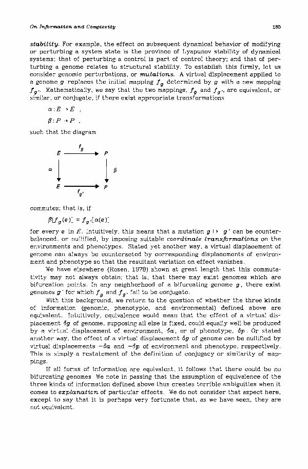
On Information and CompLezity 185

stability. For example, the effect on subsequent dynamical behavior of modifyingor perturbing a system state is the province of Lyapunov stability of dynamicalsystems: that of perturbing a control is part of control theory; and that of per­turbing a genome relates to structural stability. To establish this firmly, let usconsider genomic perturbations, or mutations. A virtual displacement applied toa genome g replaces the initial mapping 1g determined by g with a new mapping19 ,· Mathematically, we say that the two mappings, 19 and 19 ', are equivalent, orsimilar, or conjugate, if there exist appropriate transformations

a:E-·E

such that the diagram

E'g p•

·1 1(3

E ~ p

'g'commutes; that is, if

,B[fg(e)] = 19

,[a(e)]

for every e in E. Intuitively, this means that a mutation g 1-) g' can be counter­balanced, or nullified, by imposing suitable coordinate transformations on theenvironments and phenotypes. Stated yet another way, a virtual displacement ofgenome can always be counteracted by corresponding displacements of environ­ment and phenotype so that the resultant variation on effect vanishes.

We have elsewhere (Rosen, 1978) shown at great length that this commuta­tivity may not always obtain; that is, that there may exist genomes which arebifurcation points. In any neighborhood of a bifurcating genome g, there existgenomes g' for which 19 and 1g' fail to be conjugate.

With this background, we return to the questio!1 of whether the three kindsof information (genomic, phenotypic, and environmental) defined above areequivalent. Intuitively. equivalence would mean that the effect of a virtual dis­placement og of genome, supposing all else is fixed, could equally well be producedby a virtual displacement of environment, oa, or of phenotype, op. Or statedanother way, the effect of a virtual displacement og of genome can be nullified byvirtual displacements -oa and -op of e::vironment and phenotype, respectively.This is simply a restatement of the definition of conjugacy or similarity of map­pings.

If all forms of information are equivalent, it follows that there could be nobifurcating genomes. We note in passing that the assumption of equivalence of thethree kinds of information defined above thus creates terrible ambiguities when itcomes to explanation of particular effects. We do not consider that aspect here,except to say that it is perhaps very fortunate that, as we have seen, they arenot equivalent.

165 R. Rosen

Let us examine one immediate consequence of the nonequivalence of genomic,environmental, and phenotypic information, and of the considerations which cul­minate in that conclusion. Long ago (cf. von Neumann, 1951: Burks, 1966) von Neu­mann proposed an influential model for a self-reproducing automaton, and subse­quently, for automata which grow and develop. This model was based on the famoustheorem of Turing (1936), which established the existence of a universal computer(universal Turing machine). From the existence of such a universal computer, vonNeumann asserted that there must also exist a universal constructor. Basically, heargued that computation (Le. following a program) and construction (following ablueprint) are both algorithmic processes, and that anything holding for one classof algorithmic processes necessarily holds for any other class. This universal con­structor formed the central ingredient of the self-reproducing automaton.

Now, a computer acts, in the language we have developed above, through themanipulation of efficient cause. A constructor, if the term is to bear any resem­blance to its intuitive meaning, must essentially manipulate material cause. Theinequivalence of the two categories of causality, in particular manifested by thenonequivalence of environmental and phenotypic information, means that we can­not blithely extrapolate from results pertaining to efficient causation into therealm of material causation. Indeed, in addition to invalidating von Neumann'sspecific argument, we learn that great care must be exercised in general whenarguing from purely logical models (Le. from models pertaining to efficient cause)to any kind of physical realization, such as developmental or evolutionary biology(which pertain to material cause).

Thus, we realize how significant are the impacts of informational ideas, evenwithin the confines of the Newtonian paradigm, in which the categories of causa­tion are essentially segregated into separate packages. We now consider what hap­pens when we vacate the comforting confines of the Newtonian paradigm.

An Introduction to Complex Systems

Herein, I call any natural system for which the Newtonian paradigm is com­pletely valid a simple system, or mechanism. Accordingly, a complex system isone which, for one reason or another, resides outside this paradigm. We havealready seen a hint of such systems in the preceding section; for example, sys­tems whose activation-inhibition patterns Utj do not give rise to exact differen­tials LUtjdxj' However, some further words of motivation must precede a conclu­sion that such systems are truly complex (Le. reside fundamentally outside theNewtonian paradigm). We must also justify our very usage of the term complex inthis context.

What I have been calling the Newtonian paradigm ultimately devolves upon theclass of distinct mathematical descriptions which a system can have, and therelations which exist between these descriptions. As noted earlier, the basis ofsystem description arising in this paradigm is the fundamental dualism betweenstates and dynamical laws. Thus, the mathematical objects which can describenatural systems comprise a category which may be called general dynamical sys­tems. In a formal sense, it appears that any mathematical object resides in thiscategory, because the Newtonian partition between states and dynamical lawsexactly parallels the partition between propositions and production rules (rules of

On In/Drmatton and CompLexity 167

inference) which presently characterize all logical systems and logical theories.However, we argue that, although this category of general dynamical systems islarge, it is not everything, and, indeed, it is far from large enough.

The Newtonian paradigm asserts much more than simply that every image of anatural system must belong to a given category. It asserts certain relationshipsbetween such images. In particular (and this is the reductionistic content of theparadigm), it asserts that among these images there is the universal one, whicheffectively maps on all the others. Intuitively, this is the master description orultimate description, in which every shred of physical reality has an exactmathematical counterpart; in category-theoretic terms, it is much like a freeobject (a generalization of the concept of free semigroup, free group, etc.).[3]

There is still more. The ingredients of this ultimate description, by theirvery nature, are themselves devoid of internal structure; their only changeableaspects are their relative positions and velocities. Given the forces actingbetween them, as Laplace noted long ago, everything that happens in the externalworld is in principle predictable and understandable. From this perspective,everything is determined; there are no mysteries, no surprises, no errors, noquestions, and no information. This is as much true for quantum theory as for clas­sical; only the nature of state description has changed. And it applies to every­thing, from atoms to organisms to galaxies.

How does this universal picture manifest itself in biology? First, from thestandpoint of the physicist, biology is concerned with a rather small class ofextremely special (indeed, inordinately special) systems. In the theoreticalphysicist's quest for general and universal laws, there is thus not much contactwith organisms. As far as he or she is concerned, what makes organisms special isnot that they transcend the physicist's paradigms, but rather that their specifi­cation within the paradigm requires a plethora of special constraints and condi­tions, which must be superimposed on the universal canons of system descriptionand reduction. The determination of these special conditions is an empirical task;essentially someone else's business. But it is not doubted that the relationshipbetween physics and biology is the relationship between the gener~l and the par­ticular.

The modern biologist, in general, avidly embraces this perspective.[4] Histor­ically, biology has only recently caught up with the Newtonian revolution whichswept the rest of natural philosophy in the seventeenth century. The three­century lag arose because biology has no analog of the solar system; no way tomake immediate and meaningful contact with the Newtonian paradigm. Not untilphysics and chemistry had elaborated the technical means to probe microscopicproperties of matter (including organic matter) was the idea of molecular biologyeven thinkable. And this did not happen until the 1930s.

At present, there is still no single inferential chain which links any impor­tant effect in physics to any important effect in biology. This is a fact; a datum; apiece of information. How are we to understand it? There are various possibilities.Kant, long ago, argued that organisms could only be properly understood in termsof final causes or intentionality; hence, from the outset he suggested that organ­isms fall completely outside the canons of Newtonian science, which are applicableto everything else. Indeed, the essential telic nature of organisms precluded eventhe possibility that a "Newton of the grassblade" would come along, and do forbiology what Newton did for physics. Another possibility is the one we have

188 R. Rosen

already mentioned; we have simply not yet characterized all those special condi­tions which are necessary to bring biology fully within the scope of universal phy­sical principles. Yet a third possibility has developed within biology itself. as aconsequence of theories of evolution: it is that much of biology is the result ofaccidents which are in principle unpredictable and hence governed by no lawsat all.[5] In this view biology is as much a branch of history as of science. Atpresent, this last hypothesis lies in a sort of doublethink relation with reduction­ism; the two are quite inconsistent, but do allow modern biologists to enjoy thebenefits of vitalism and mechanism together.

Yet a fourth view was expressed by Albert Einstein, who wrote in a letter toLeo Szilard: "One can best appreciate, from a study of living things, how primitivephysics still is".

So, the present prevailing view in biology is that the Newtonian canons areindeed universal, and we are lacking only knowledge of the special conditions andconstraints which distinguish organisms from other natural systems within thosecanons. One way of describing this with a single word is to assert that organismsare complex. This word is not well defined, but it does connote several things. Oneof these is that complexity is a system property, no different from any other pro­perty. Another is that the degree to which a system is complex can be specifiedby a number, or set of numbers. These numbers may be interpreted variously asthe dimensionality of a state space, or the length of an algorithm, or as a cost intime or energy incurred in solving system equations.

On a more empirical level, however, complexity is recognized differently, andcharacterized differently. If a system surprises us, or does something we have notpredicted, or responds in a way we have not anticipated; if it makes errors; if itexhibits emergence of unexpected novelties of behavior, we also say that the sys­tem is complex. In short, complex systems are those which behave counter­intuitively.

Sometimes, of course, surprising behavior is simply the result of incompletecharacterization; we can then hunt for what is missing, and incorporate it into oursystem description. In this way, the planet Neptune was located from unexplaineddeviations of Uranus from its expected trajectory. But sometimes this is not thecase; in the apparently analogous case of the anomalies of the trajectory of theplanet Mercury, for instance, no amount of fiddling within the classical scenariosucceeded and only a massive readjustment of the paradigm itself (via generalrelativity) availed.

From these few words of introduction, we can conclude that the identificationof complexity with situations where the Newtonian paradigm fails is in accord withthe intuitive connotation of the term, and is an alternative to regarding as com­plex any situation which merely is technically difficult within the paradigm.

Now let us see where information fits into these considerations. We recallthat information is the actual or potential response to an interrogative, and thatevery interrogative can be put into the variational form: If oA, then oB? TheNewtonian paradigm asserts, among other things, that the answers to such interro­gatives follow from dynamical laws superimposed on manifolds of states. In theirturn, these dynamical laws are special cases of equations of state, which link orrelate the values of system observables. Indeed, the concept of an observable was

On Information ana CompLexity 189

the point of departure for our entire treatment of system description andrepresentation (cf. Rosen, 1978); it was the connecting link between the world ofnatural phenomena and the entirely different world of formal systems which weuse to describe and explain.

However, the considerations we have developed above suggest that this worldis not enough. We require also a world of variations, increments, and differentialsof observables. It is true that every linkage between observables implies acorresponding linkage between differentials, but as we have seen, the converse isnot true. We are thus drawn to the notions that a differential relation is a general­ized linkage and that a differential form is a type of generalized observable. A dif­ferential form which is not the differential of an observable is thus an entitywhich assumes no definite numerical value (as an observable does), but which canbe incremented.

If we do think of differential forms as generalized observables. then we mustcorrespondingly generalize the notion of equation of state. A generalized equationof state thus becomes a linkage or relation between ordinary observables and dif­ferentials or generalized observables. Such generalized equations of state are thevehicles which answer questions of our variational form: If 6A, then tiB?

But as we have repeatedly noted, such generalized equations of state do notusually follow from systems of dynamical equations, as they do in the Newtonianparadigm. Thus, we must find some alternative way of characterizing a system ofthis kind. Here is where the informational language introduced above comes to thefore. Let us recall, for instance, how we defined the activation-inhibition net­work. We found a family of functions u ij (Le. of observables) which could bethought of in the dynamical context as modulating the effect of an increment dXj

on that of another increment df i' That is, the values of each observable. u ij •

measure precisely the extent of activation or inhibition which x j exerts on therate at which xi is changing.

In this language. a system falling outside the Newtonian paradigm (Le. a com­plex system) can have an activation-inhibition pattern, just as a dynamical (Le.simple) system does. Such patterns are still families of functions (observables),u ij ' and the pattern itself is manifested by the differential forms

{.)i = 2;uij dxj

But in this case, there is no global velocity observable. f i' that can be inter­preted as the rate of change of xi: there is only a velocity increment. It shouldbe noted explicitly that u ij ' which define the activation-inhibition pattern, neednot be functions of xi alone, or even functions of them at all. Thus, the differen­tial forms which arise in this context are different from those with whichmathematicians generally deal, and which can always be regarded as cross sectionsof the cotangent bundle of a definite manifold of states.

The next level of information is the agonist-antagonist pattern, Uijk' In thecategory of dynamical systems, this is completely determined by theactivation-inhibition pattern, and can be obtained from the latter by differentia­tion:

190 R. Rosen

In our world of generalized observables and linkages, U tjle are independent ofU tj ' and must be posited separately; in other words, complex (non-Newtonian) sys­tems can have identical activation-inhibition patterns, but quite differentagonist-antagonist patterns.

Exactly the same considerations can also be applied to every subsequentlayer of the informational hierarchy; each is now independent of the others, andso must be posited separately. Hence a complex system requires an infinitemathematical object for its description.

We cannot examine herein the mathematical details of the considerationssketched so briefly above. Suffice it to say that a complex system, defined by ahierarchy of informational levels of the type described, is quite a different objectto a dynamical system. For one, it is quite clear that there is no such thing as aset of states, assignable to such a system once and for all. From this alone, wemight expect that the nature of causality in such systems is vastly different towhat it is in the Newtonian paradigm; we come to this in a moment.

The totality of mathematical structures of the type we have defined aboveforms a category. In this category the class of general dynamical systems consti­tutes a very small subcategory. We are suggesting that the former provides a suit­able framework for the mathematical imaging of complex systems, while the latter,by definition, can only image simple systems or mechanisms. If these considera­tions are valid (and I believe they are), then the entire epistemology of ourapproach to natural systems is radically altered, and it is the basic notions ofinformation which provide the natural ingredients.

There is, however, a profound relationship between the category of generaldynamical (I.e. Newtonian) systems, and the larger category in which it is embed­ded. This can only be indicated here, but it is important indeed. Namely, there is a;>recise sense in which an informational hierarchy can be approximated, locallyand temporarily, by a general dynamical system. With this notion of approximationthere is an associated notion of limit, and hence of topology. Using these ideas, itcan be shown that what we call the category of complex systems is the completion,or limiting set, of the category of simple (I.e. dynamical) systems.

The fact that complex systems can be approximated (albeit locally and tem­porarily) by simple ones is crucial. It ex;>lains precisely why the Newtonian para­digm has been so successful, and why, to this day, it represents the only effectiveprocedure for dealing with system behavior. But in general, it is apparent that itcan usually supply only approximations, and in the universe of complex systemsthis amounts to re;>lacing a complex system with a simple subsystem. Some of theprofound consequences are considered in detail in Rosen (1978).

This relationship between complex systems and simple ones is, by its verynature, without a reductionistic counter;>art. Indeed, what we presently under­stand as physics is seen in this Light as the science of simple systems. Therelation between physics and biology is thus not at all the relation of general to';)e.rticulac; in fact, quite the contrary. It is not biology, but physics, which is toospecial. We can see from this perspective that biology and physics (I.e. contem­jJorary physics) develop as two divergent branches from a theory of complex sys­tems, which as yet can be glimpsed only very imperfectly.

The category of simple systems is, however, still the only one that we knowhow to use. But to study complex systems by means of approximating simple sys­tems resembles the position of early cartographers, who were attempting to map a

On Informa.tion a.nd CompLexity 191

sphere while armed only with pieces of planes. Locally, and temporarily, theycould do very well, but globally, the effects of the topology of the sphere becomeprogressively important. So it is with complexity; over short times and only a fewinformational levels, we can always make do with a simple (Le. dynamical) picture.Otherwise, we cannot; we must continually replace our approximating dynamicswith others as the old ones fail. Hence another characteristic feature of complexsystems; they appear to possess a multitude of partial dynamical descriptions,which cannot be combined into one single complete description. Indeed, in earlierwork (Rosen, 1977), we took this as the defining feature of complexity.

I add a brief word about the status of causality in complex systems, andabout the practical problem of determining the functions which specify theirinformational levels. Complex systems do not possess anything like a state setwhich is fixed once and for all. Also, the categories of causality becomeintertwined in a way which is not possible within the Newtonian paradigm. Intui­tively, this follows from the independence of the infinite array of informationallayers which constitutes the mathematical image of a complex system. Variation ofany particular magnitude connected with such a system typically manifests itselfindependently in many of these layers, and thus reflects itself partly as materialcause, partly as efficient cause, and even partly as formal cause in the resultantvariation of other magnitudes. We feel that it is, at least for the most part, thisinvolvement of magnitudes simultaneously in each of the causal categories whichmakes biological systems so refractory to the Newtonian paradigm.

Also, this intertwining of the categories of causation in complex systemsmakes the direct interpretation of experimental results of the form: If c5A, thenc5B, extremely difficult. If we are correct so far, such an observational result asit stands is far too coarse to have any clear-cut meaning. In order to be meaning­ful, an experimental proposition of this form must isolate the effect of a variationc5A on a single informational level, keeping the others clamped. As might beappreciated, this will in general not be an easy task. In other words, the experi­mental study of complex systems cannot be pursued with the same tools and ideasthat are appropriate for simple systems.

One final conceptual remark is also needed. As mentioned earlier, theNewtonian paradigm has no room for the category of final causation. This categoryis closely linked to the notion of anticipation, which in turn is linked to the abilityof systems to possess internal predictive models of themselves and their environ­ments, which can be utilized for the control of present actions. We have argued atgreat length elsewhere (cf. Rosen, 1984) that anticipatory control is indeed a dis­tinguishing feature of the organic world. and have described some of the uniquefeatures of such anticipatory systems. Herein we have shown that for a system tobe anticipatory, it must be complex. Thus, our entire treatment of anticipatorysystems becomes a corollary of complexity. In other words, complex systems canadmit the category of final causation in a perfectly rigorous, scientifically accept­able way. Perhaps this alone is sufficient recompense for abandoning the comfort­ing confines of the Newtonian paradigm, which has served so well over the centu­ries. It will continue to serve us well, provided we recognize its restrictions andlimitations. as well as its strengths.

192

Notes

R. Rosen

[1] Newton's original particle mechanics, or vectorial mechanics, is hard to apply tomany practical problems, and was early on (through the work of people like Eulerand Lagrange) transmuted into another form, generally called analytical mechan­ics. This latter form is usually used to deal with extended matter (e.g. rigidbodies). In particle mechanics, the rigidity of a macroscopic body is a consequenceof interparticle forces, which must be explicitly taken into account in describingthe system. Thus, if there are N particles in the system (however large N may be)there is a phase space of 6N dimensions, and a set of dynamical equations whichexpresses for each particle the resultant of all forces experienced by that parti­cle. In analytical mechanics, on the other hand, any rigid body can be completelydescribed by giving only six configurational coordinates (e.g. the coordinates ofthe center of mass, and three angles of rotation about the center of mass), how­ever many particles it contains. From the particulate approach the internal forceswhich generate rigidity are replaced by constraints; supplementary conditions onthe configuration space which must be identically satisfied. Thus, the passage fromparticle mechanics to analytical mechanics involves a partition of the forces in anextended system into two classes: (a) the internal or reactive forces, which holdthe system together, and (b) the impressed forces, which push the system around.The former are represented in analytical mechanics by algebraic constraints, thelatter by differential equations in the configuration variables (six for a rigidbody).

A system in analytical mechanics may have additional constraints imposedupon it by specific circumstances; for example, a ball may roll on a table top. Itwas recognized long ago that these additional constraints (which, like all con­straints, are regarded as expressing the operation of reactive forces) can be oftwo types, which were called by Hertz holonomic and nonholonomic. Both kinds ofconstraints can be expressed locally, in infinitesimal form, as

nl: tit (x1,···,xn )dzt = 0

t '" 1

where Xl"'" X n are the configuration coordinates of the system. For a holonomicconstraint, the above differential form is exact; that is, the differential of someglobal function <p(x 1'"'' x n ) is defined over the whole configuration space. Thus,the holonomic constraint translates into a global relation

<p(x 1"'" Xn ) = constant .

This means that the configurational variables are no longer independent, and thatone of them can be expressed as a function of the others. The constraint thusreduces the dimension of the configuration space by one, and therefore reducesthe dimension of the phase space by two.

A nonholonomic constraint, on the other hand, does not allow us to eliminate aconfigurational variable in this fashion. However, since it represent'l a relationbetween the configuration variables and their differentials, it does allow us toeliminate a coordinate of velocity, while leaving the dimension of the configurationspace unaltered. That is, a nonholonomic constraint serves to eliminate one degreeof freedom of the system. It thus also eliminates one dimension from the space ofimpressed forces which can be imposed on the system without violating the con­straint.

Similarly, if we impose r independent nonholonomic constraints on our sys­tem, we (a) keep the original dimension of the configuration space; (b) eliminate rcoordinates of velocity, and thus reduce the dimensionality of the phase space byr; and (c) similarly, reduce by r the dimensionality of the set of impressed forceswhich can be imposed on the system.

On Iftjbrm~t1.oft~ftlt Complez1.tll 193

Let us express these facts mathematically. A nonholonomic constraint can beexpressed locally in the general form

tp[Zl, ... ,Zn. ~1 ..... ~: ] =0

which can (locally) be solved for one of the velocity coordinates (dz1 / dt, say).Thus, it can be written in the form

~1 = t[Zl' z2' .... zn. d;t2 .... , d;; ]

= >I'(zl' a)

where we have written a. = (z2'"'' dzn / dt). [At this point the reader is invited tocompare this relation with equation (7.6) in the main text.]

Likewise. if there are r nonholonomic constraints, these can be expressedlocally by r equations

dzt/dt =tt(zl' .... zr.a.) i =l..... r

where now a is the vector (zr +l, ... ,zn' dZr +l/dt ,... ,dzn /dt). These equations ofconstraint, which intuitively arise from the reactive forces holding the systemtogether, now become more and more clearly the type of equations we always use todescribe general dynamical or control systems.

Now what happens if r = n? In this case. the constraints leave us only oned.egree oj freed.om; they d.etermine a vector field. on the configuration space.There is in effect only one impressed. force that can be imposed on such a system,and its only effect is to move the system; once moving, the motion is determinedentirely by the reactive forces. and not by the impressed. force. Mathematically,the situation is that of an autonomous dynamical system, whose manifold of states isthe conJ'i,guration space of the original mechanical system.

This relationship between dynamics and mechanics is quite different from theusual one. in which the manifold of states is thought of as generalizing the mechani­cal notion of phase, and the equations of motion as generalizing the impressed.force. In the above interpretation. however, it is quite different; the manifold ofstates correspond now to mechanical conJ'i,gurations. and the equations of motioncome from the reactive forces.

[2] The reader should be most careful not to confuse two kinds of propositions, whichare equivalent mathematically but completely different epistemologically andcausally. On the one hand, we have a statement like

dz/dt =fg(z, a) .

This is a local proposition. linking a tangent vector or velocity dz / dt to a statez. a genome g. and a control a. Each of these quantities is derived from observ­abIes assuming definite numerical values at any instant of time, and it is theirvalues at a common instant which are related by this proposition.

On the other hand, the integrated form of these dynamical relations ist

z(t) = J fg[z,a(T)]dT .to

This relationship involves time e:r:plicitly and links the values of observables atone instant with values (assumed by these and other observables) at otherinstants.

Each of these epistemically different propositions has its own causal struc­ture. In the first, we treat the tangent vector dz /dt as effect and define itscausal antecedents as we have done. In the integrated form, on the other hand, wetake z (t) as effect and find a correspondingly different causal structure. In gen­eral, the mathematical or logical equivalence of two expressions of linkage or

194 R. Rosen

relationship in physical systems does not at all connote that their causal struc­tures are identical. This is merely a manifestation of what was discussed earlier,that the mathematical language we use to represent physical reality hasabstracted away the very basis on which such causal discriminations can be made.

[3] It should be recognized that this reductionistic part of the Newtonian paradigm canfail for purely mathematical reasons. If it should happen that there is no way toeffectively map the master description onto some partial description, then this isenough to defeat a reductionistic approach to those system behaviors with whichthe partial description deals. This is quite a different matter from the one we areconsidering here, in which no Newtonian master description e:r:ists, and the pro­gram fails for epistemological reasons, rather than mathematical ones.

[4] This statement is not simply my subjective assessment. In 1970 there appeared avolume entitled Biology and the Future of Man, edited by Philip Handler (1970),then President of the National Academy of Sciences of the USA. The book went togreat lengths to assure the reader that it spoke for biology as a science; that in itbiologists spoke with essentially one voice. At the outset, it emphasized that thevolume was not prepared as a (mere) academic exercise, but for serious pragmaticpurposes:

Some years ago, the Committee on Solence and Public Polley of the NationalAcademy of Sciences embarked on a series of 'surveys' of the scientific dis­ciplines. Each survey was to commence with an appraisal of the 'state of theart'.... In addition, the survey was to assess the nature and strength of ournational apparatus for continuing attack on those major problems, e.g., thenumbers and types of laboratories, the number of scientists In the field, thenumber of students, the funds available and their sources, and the majorequipment being utilized. Finally. each survey was to undertake a projectionof future needs for the national support of the discipline In question toassure that our national effort In this regard Is optimally productl ve....

To address these serious matters, the Academy proceeded as follows:

.... Panels of distinguished scientists were assigned subJects.... Each panelwas glven a general charge... as follows:

The prime task of each Panel Is to prOVide a pithy summary of the status ofthe specific sub-field of science which has been assigned. This shOUld be aclear statement of the prime scientific problems and the major questionscurrently confronting Investigators In the field. Included should be an Indi­cation of the manner In whloh these problems are being attacked and howthese approaohes may change within the foreseeable future. What trends canbe visualized for tomorrow? What lines of Investigation are likely to sub­side? Which may be expected to advance and assume greater Importance? ...Are the questions themselves ... likely to change significantly? ... Havingstated the major questions and problems, how close are we to the answers?The sum of these discussions, panel by panel, should constitute the equivalentof a complete overview of the highlights of current understanding of the LifeSciences.

There were twenty-one such Panels established, spanning the complete gamutof biological sciences and the biotechnologies. The recruitment for these Panelsconsisted of well over 100 eminent and influential biologists, mostly members of theAcademy. How the panelists themselves were chosen is not indicated, but there isno doubt that they constituted an authoritative group.

In due course, the Panels presented their reports. How they were dealt withis described in colorful terms:

.... In a gruelling one week session of the Survey Committee... each reportwas merciLessLy exposed to the criticism of all the other members.... Eachreport was then rewritten and subjected to the search.ing, sometimes SCClth.­ing, criticisms of the members of the parent Committee on Science and Public

On Information and CompLexity

Polley. The reports were again revised In the llght of this exercise. Finally,the Chairman of the Survey Committee... devoted the summer of 1968 to thefinal editing and revising of the final work.

195

Thus we have good grounds for regarding the contents of this volume as con­stituting a truly authoritative consensus, at least, as of 1970. There are no minor­ity reports; no demurrals; biology does indeed seem guaranteed here to speak withone voice.

What does that voice say? Here are a few characteristic excerpts:

The theme of this presentation Is that llfe can be understood In terms of thelaws that govern and the phenomena that characterize the Inanimate, physi­cal universe and, Indeed, that at Its essence llfe can be understood onLy Inthe language of chemistry. [emphasis added]

A little further along, we find this:

Untll the laws of physics and chemistry had been eluoldated, it was not pos­sibLe even to formuLate the Important, penetrating questions concerning thenature of llfe.... The endeavors of thousands of llfe scientists... have gonefar to document the thesis... (that) llvlng phenomena are Indeed Intell1glbleIn physical terms. And although muoh remains to be learned and understood,and the detalls of many processes remain elusive, those engaged In suchstudies hold no doubt that answers will be forthcoming In the reasonablynear future. Indeed, onLy two major questions remain enshrouded In a cloakof not quite fathomable mystery: (1) the origin of llfe... and (2) themind-body problem... yet (the extent to which biology Is understood) evennow constitutes a satisfying and exciting tale. [emphases added]

Still further along, we find things like this:

Whlle gLorying In how far we have come, these chapters also reveal howlarge Is the task that lles ahead.... If (molecular biology) Is exploited withVigor and understanding... a shining, hopeful future lles ahead. [emphasisadded]

And this:

Molecular biology prOVides the closest Insight man has yet obtained of thenature of llfe - and therefore, of himself.

And this:

It will be evident that the huge Intellectual triumph of the past decade will, Inall llkellhood, be surpassed tomorrow - and to the everlasting benefit ofmankind.

It is clear from such rhapsodies that the consensus reported in this volume is notonly or even mainly a scientific one; it is an emotional and aesthetic one. Andindeed, anyone familiar with the writings of Newton's contemporaries and succes­sors will recognize them.

The volume to which we have alluded was published in 1970. But it is most sig­nificant that nothing fundamental has changed since then.

[5] In the inimitable words of Jacques Monod (1971, pp 42-43):

We can assert today that a universal theory, however oompletely successfulIn other domains, could never encompass the biosphere, Its structure and Itsevolution as phenomena deducible from first principles.... The thesis I shallpresent... Is that the biosphere does not contain a predictable class ofobjects or events but constitutes a particular occurrence, compatible withfirst principles but not deducible from these principles, and thereforeessentiaLLy unpredictabLe. [emphasis added]

196

References

R. Rosen

Burks, A. (1966) Theory of Self-Reproducing Automata (Urbana, 1L: University of Illi­nois Press).

Handler, P. (Ed) (1970) Biology and the Future of Man (Oxford: Oxford UniversityPress).

Higgins, J. (1967) Oscillating chemical reactions. J. Ind. IJc Eng. Chem. 59: 18-62.Monod, J. (1971) Chance and Necessity (New York: Alfred A. Knopf).von Neumann, J. (1951) The general and logical theory of automata, in L.A. Jeffress (Ed)

Cerebral Mechanisms in Behavior (New York: John Wiley & Sons) pp 1-41.Rosen, R. (1977) Complexity as a system property. Int. J. General Systems 3: 227-32.Rosen, R. (1978) Fundamentals of Measurement and Representation of Natural Sys­

tems (New York: Elsevier).Rosen, R. (1979) Some comments on activation and inhibition. Bull. Math. Biophysics 41:

427-45.Rosen, R. (1983) The role of similarity principles in data extrapolation. Am. J. Physiol.

244: R591-9.Rosen, R. (1985) Anticipatory Systems (London: Pergamon Press) in press.Shannon, C. and Weaver, W. (1949) The Mathematical Theory oJ Communication

(Urbana, 1L: University of Illinois Press).Turing, A.M. (1936) On computable numbers. Proc. London Math. Soc. Ser. 2, 42: 230-65.

CHAPTER 8

Organs and Tools: A Common Theory of Morphogenesis

Rene Thorn

Introduction: Toward a Comprehensive Biological Theory

At the beginning of the sixteenth century, people began to anatomize deadbodies and discovered organs for which the putative function had to be found. Thesimplest method of establishing this was to associate the organ with a tool, whichapparently naive procedure led, nevertheless, to striking successes. Within thatcentury, Harvey showed the heart to be a pump that sent blood through naturalpipes, the blood vessels. The skeleton (bones. joints, and muscles) provided obvi­ous mechanical interpretations (a member acting as a lever, for instance); and thelungs were compared to a pair of bellows (with the obvious omission of the funda­mental physiological function of gas exchange between air and blood). All thesemechanical analogies led to Descartes' theory of the animal machine. It was onlywith our noblest organ. the brain (the seat of the soul). that these analogicalexplanations met with difficulties: How could consciousness and thinking be gen­erated inside this apparently amorphous gray or white substance? But themechanical imagery was to achieve, around 1950, its most notable success. Thealmost simultaneous appearance, in the middle of the twentieth century, of com­puters and molecular biology developed the idea that the genetic material, DNA.was the analogue of a computer program for the development of an adult organismfrom an egg. This interpretation offered a new, important breakthrough: previ­ously the mechanical analogy had constantly raised the problem of biological finai­ity. How could all these organs, so beautifully adapted to their function and ofsuch a huge efficiency, be formed, apparently by themselves. during embryologicaldevelopment? Was it not necessary to postulate the assistance of a "genius ", ademiurge who had to direct and control the whole process of epigenesis? The pro­position that the complete structure of the organism might be encoded in thegenomic nucleotide sequence of DNA solved the problem: one had only to admitthat DNA, playing the role of the demiurge, directed the full development of theembryo, exactly as an engineer dictates orders to his or her subordinates in amanufacturing plant. Thus, teleology could be rendered more acceptable under the

198 R. Thom

new term of teleonomy. This idea gained acceptance as soon as it was discoveredthat the traduction mechanism, DNA ... protein, was effectively a code, in thetechnical sense of the word; to any triple of nucleotides there corresponds onlyone amino acid. But, in the initial case of metazoa embryonic development, thesituation is entirely different: one has to understand how the genetic informationsupposedly included in DNA can render itself in the three-dimensional (3-D)organic structure of the embryo (and later of the adult). (Here I am referring tothe Metazoa; the case of Procaryotes is somewhat different.) As a result, allmodern biological thought has been trapped in the fallacious homonym associatedwith the phrase "genetic code", and this abuse of language has resulted in a stateof conceptual sterility, out from which there is little hope of escape.

To achieve some progress in solving this difficulty, only a major theoreticaljump will be of any help. And theory cannot exist - in biology no less than in anyother discipline - without introducing imaginary entities. After all, life itself, inthe usual reductionist view, cannot be anything other than an imaginary concept.Thus, in the organ-tool conceptualization, it may be more sensible to reverse thesense of the explanation; instead of explaining the organ by the tool, could we notexplain the tool by the organ? This has already been suggested by many vitalistphilosophers, such as Bergson. Could the intuitive imagination which led Homofaber to build his extraordinarily efficient tools - centuries before the appear­ance of modern science - be none other than the manifestation through phylo­genetic evolution of some biological unconsciousness? A simple idea can be takenhere as evidence: the tool. generally, extends the action, and the action, in itsessential motor structure, is genetically inherited. We have here to reconsider theLamarckian axiom: function creates the organ. Not, as is often trivially stated,that organs are created and develop as the result of the frequent performance ofa function, but in a more abstract, platonic sense. All the regulatory properties ofan organic structure rely on some geometric properties of a "figure of regulation"which lies in some abstract space of metabolic activities. A function is then aregulatory apparatus of a formal, dynamic nature insuring homeostasis of somephysiologically important character (or parameter), such as chemical energy con­tent, oxygen content, organic waste content, etc. The performance of such a func­tion may involve a wide variety of physicochemical agents as well as the mostdiverse organs. When all these functions perform correctly, they insure canaliza­tion of the metabolic state of the system around a specific attractor (the figure ofregulation).

The aim of theoretical biology is to describe (with the utmost accuracy possi­ble) this geometric object. We are certainly still very far from this, but as anapproximate procedure, we may try to give local descriptions associated with aspecific function, using the data of partial models of the following type. If the fig­ure of regulation is described as an invariant, closed object of flow X in a space ofvery high dimension 0, a function may be given by an auxiliary dynamic (M; Y),

where Y is a flow in a phase space M of low dimension, and we have a smooth mapF(Oz) ... M such that for any :z: E: 0, with y = F(:z:), the image vector F'(X;:z:) isvery near Y(y). Moreover, the image dynamics (M; Y) have to be algebraically sim­ple (as in catastrophe theoretic modeling). The local coordinates in Y have biologi­cal meaning; they insure that the semiotic character of life is the most importantvalue to be defended against the potentially deadly threats of external stresses.[Here we have the axiologic character of these imaginary entities. frequently

OrgCJns end ThoLs 199

described mathematically by a potential function, following Kergosien's terminol­ogy (1984).] Of course, the use of such imaginary entities produces difficult philo­sophical and methodological problems. In fundamental physics, most basic notions(such as mass, force, fields, etc.) are also imaginary, but their existence is madelegitimate by their implication in highly accurate quantitative laws. In biology wecannot expect such a justification; but, at least, we may introduce our imaginaryentities in to qualitatively stable models. In the same way as physical laws arefrequently the results of symmetry constraints, we may try to impose as rigorouslyas possible constraints for the spatiotemporal propagation of our entities. Practi­cally, all these constraints arise as the consequences of a single principle, theprinciple of locality, which can be stated as follows: any local process inside aliving being has to be explained as a result of only local deterministic processes.Action at a distance is prohibited (e.g., pure magic).

In its most general formulation, the principle of locality could be stated notonly with respect to the usual space-time dimensions, but also to all semiotic (ima­ginary) spaces in which our imaginary entities are embodied. However, this wouldexclude any kind of qualitative discontinuity in the behavior of such entities; sucha restriction is too stringent and one has to allow that at exceptional loci discon­tinuities of a qualitative character may occur (catastrophes), in the same way assound propagation has to accept the presence of shock waves. But, in such cases,the discontinuities themselves have to be explained in terms of local deterministicprocesses (this justifies the importance of catastrophe theoretic formalism).

Salient Forms and Pregnances

The concepts used in such analyses are of two kinds:

(1) Salient forms, that is forms which are defined by a sharp boundary in theirbackground space. Molecules, cells, organs, and organisms are salient forms,with well-defined spatiotemporal localization. Most of these forms are clearlyindividualized and in space any two have to be disjoint (impenetrability).

(2) Pregnances denote all field-like entities; they are not localized so two dis­tinct pregnances may be present at the same point of space-time withoutinteracting. Pregnances propagate in space, according to local deterministicprinciples [for instance, partial differential equations (PDE) for physicalfields]. Any pregnance involves some energy content and, as such, any pro­pagating pregnance is also an energy flux. (In some sense, the concept ofenergy is the most general physical pregnance.) Biological pregnances aresometimes subjectively defined (as life, fear, etc.); objectively, they pro­pagate in space-time via material support or appropriate salient forms (thesupport of these forms may be material or field-like; olfactory signals are ofthe first kind, visual and auditory of the second).

Interactions between salient forms and pregnances may be described as fol­lows (cf. Thom, 1983). Pregnances emanate from salient forms called source forms.They may invest other salient forms, in which they create a change of internalstate with, sometimes, perceptible effects (the so-called figurative effect); gen­erally, invested salient forms become secondary, induced source forms for thesame pregnance. Subjective pregnances propagate from salient form to salient

200 R. 7ll.om

form by two modes of action; action by contiguity (contact) and action by similar­ity. Objective pregnances propagate only by contact (the axiom of locality). Usingthis ontology of salience and pregnances, we may establish the following classifica­tion of local processes:

(1) A salient form invested. by a pregnance. This may be subjective; for exam­ple, a subject under the influence of fear communicated by nearby subjects.Or it may be objective, such as excitation of an atom (salient form) by anelectromagnetic field (a physical pregnance); microbial contagion of an animalis another example, the contagious disease being here an objective preg­nance. The fact that the pregnance is carried by specific salient forms (thebacteria) is no reason to exclude a contagious disease from the pregnanceconcept.

(2) Emission of a pregnance by a salient form. An infested individual may pro­pagate a contagious disease. In fact, it should be realized that in order for aform to be salient, it has to be carried to an observer by a physical field(such as light or sound).

(3) Interaction of a pregnance with a salient form. Here we are basically con­cerned with physical flows that satisfy, locally, the invariance of the kineticmomentum. If we immerse a solid (s) in such a flow, then the topology of theflow may be drastically changed according to the position of s inside the flow.This type of interaction is the basis of the notion of preprogram, developedbelow.

(4) Pregnance-pregnance interactions. Little is known in general about suchinteractions, except the case where the pregnances are described by poten­tial functions on the same space, where the catastrophe theoretic formalismmay be valid. In particular, a pregnance may interact with itself in such away as to create shocks (that is salient forms), but these rarely materializeas independent entities.

(5) Interactions between salient forms. I believe that such interactions canalways be described as an exchange of pregnances between the forms.

Interactions of type (5) are the only ones recognized in modern biology (forinstance, communications between cells). The logicist ideal is to eliminate preg­nances and reduce them to contiguity processes that involve only contact, absorp­tion, or emission of material bodies. But physical fields are not matter andbiochemical interpretation of the great pregnances (the effects) is still very farfrom being achieved.

As said earlier, any physiological function has, in practice, a large number ofbiochemical carriers (even inside the same individual); this renders the biochemi­cal interpretation of pregnances very difficult, although a complete theory shouldalso explain the variations of biochemical support of a given function within, forinstance, the animal kingdom. Thus, a comparative evolutionary physiology isneeded, which should parallel, and complete, the comparative evolutionaryembryology. Here, quite certainly, historical events played an important role, andaccounting for their importance would require much painful study.

Among the imaginary entities that must be introduced are the classical epi­genetic gradients of embryology. Nobody knows the biochemical basis for ananimal's cephalocaudal gradient, but nobody can doubt its importance. On this

Orga""s a""a Thots :lO1

basis alone, the theoretical introduction of pregnances seems to me in need of nofurther justification. But, of course, in each specific case one has to find con­straints to the propagation of pregnances. Do they need specific salient forms toinvest? What kind of partial differential equation, if any, must they satisfy to pro­duce smooth propagation? If the physicochemical basis of the pregnance is known(molecular diffusion, electromagnetic fields, etc.) such constraints may be esta­blished. If the basis is unknown, one may have to rely only on a locality axiom, act­ing in a purely qualitative way. In such cases, it may be impossible to build a modelin the usual quantitative sense of the word, but we may, nevertheless, arrive at ametaphor which, while not allowing strict control of the situation, could bringabout a better understanding of the phenomena.

The Notion of Preprogram

In my book Structural Stability and Morphogenesis (Thom, 1972) I pro­posed that the major accidents of early embryology (gastrulation, etc.) could beexplained by mechanisms of type (4), where initially we have only epigenetic gra­dients unfolding some singularity of a potential that is of metabolic origin. Such aconcept is acceptable only in a static situation, in which the inner fluxes ofenergy within the embryo may be neglected. As soon as some inner circulationarises, then kinetic variations of these fluxes have to be taken into consideration;this corresponds to the somewhat mysterious process denoted internalization ofan external 'Variable in my previous work (Thom 1972). This is why any coherenttheory of morphogenesis has to account for how a propagative flux of energy canbe modified in its topology under a variation of the boundary constraints. This isthe object of the classical obstacle problem in PDE theory (see, for instance,Arnol'd's book, Catastrophe Theory, 1984). I propose to summarize all that weneed in the following metatheorem.

We consider a domain U in some Euclidean space R"" +1(x; y); with x aspecific, real coordinate, and y E: R"". Suppose that the domain U meets the slicea ,..;; x ,..;; 1 along some set B and suppose that U is crossed by an energy (ormaterial) flow which propagates in the sense of increasing x. This flow emanatesfrom a source situated distantly in the negative x half-space. We suppose that theboundary BB can be subjected to a deformation

G: B x I ~ R"" +1, a < x < 1 ,

depending on the parameter s E: I, leaving the edges fixed, B r'I [x = 0, 1]. Letm (s; y), y E: R"", be the asymptotic density of the energy flow for a value s of thedeforming parameter [if s is time, then the deformation G(s) is supposed to beinfinitely slow with respect to the speed of the flow]. For any s, the boundaryG (s) is impenetrable to the flow, which must always be tangent to the boundary.Let C be the set of critical values of the smooth, real-valued function m (s; y) inthe plane (s; m). Then, by the genericity assumption, the set C is a smooth curvewith normal crossings as the only singularities, and its projection on the s-axisadmits only fold points (f) as critical points (Figure 8.1). Proof of thismetatheorem requires showing that the associated map F which transforms thefunction space of the deformation G (s) into the function space of the densitym (s; y) is sufficiently surjective to permit transversality of the m functionswhich are not generic. I do not know to what extent theorems of this type are

202 R. Thom

found in the current literature. It should be observed, also, that the spatialframework in which this theorem was stated may allow any kind of interpretation,whatever the propagating process we began with.

m

r s

Figure 8.1 Arcs of maxima (-); arcs of index n -1(--); 1" = slopping poinl.

In applications to morphogenesis, U is the usual domain of 3-D Euclideanspace. We consider, on the curve C, those arcs J associated with the maxima of thedensity m (s; y), and we restrict ourselves to only fairly sharp maxima, with verylow intervening thresholds. The standard fold point of C is the junction of a J-arcwith an arc of index one in the density m (s; y). If the parameter s denotes time,then for a value sO for which a maximum lJ.(s) disappears. we have at the dispari­tion point two possible situations:

(1) The disparition point (sO; Y) is a fold point of C; there the maximum fJ- of mcoincides with a saddle of index one, according to a local model of the type

m(s;Y) =m(so;y) + (s - sO)Y1 + yf + L (Yj)2l<j <11.-1.

for local coordinates Y l' Yj in Y, and m (sO; Y) -;. O. Then the fold point inthe (s; m) plane is a flex point (with horizontal tangent) of the graph of thefunction m (s 0; Y 1)' Hence it belongs to the basin of some other maximum 1" ofm(so; Y1; Yj)' whose local flow captures the disappearing flow (Figure 8.2).

(2) At the disparition point (sO; Y). the local intensity m (so; Y) vanishes. This is,strictly speaking, not a generic situation, but it is of utmost practical impor­tance; it corresponds to the task of stopping entirely the local flow.

These two situations can be symbolized by the two graphs 1A and 1B in Figure8.3. By reversing the sense of time, we obtain the two symmetric morphologies 2Aand 2B in Figure 8.3. These four morphologies playa fundamental role in classify­ing organs and tools according to their main functions. In the technical world, oneof the most frequent preprograms occurs when a solid (s) is immersed in a materialflow; here the control space U may be the full 6-D space describing all positions ofU. If we consider k-D families of the positions of s we may obtain in such a controlspace higher singularities than those described above. For instance, in a 2-D U we

Orgllns lind ThoLs

m T

203

y y

Figure 8.2 Capture of a disappearing maximum j.J. by a higher maximum T.

1A: Confluence of the two flows

2A: Ramification of a flow

Figure 8.3 Morphologies lA, lB, 2A, and 2B.

1B: End of a flow

2B: Birth of a flow

may have points where a flow may possess a triple ramification (stably in lJ), butusually the solid s is constrained in a low-dimensional family of positions.

This notion of preprogram appears as a dynamical metaphor for the classicnotion of gatekeeper due to Kurt Lewin (1951), the founder of topological psychol­ogy; that is. an individual whose position in a society allows him or her to modifydeeply the structure and the intensity of some particular economic (or communica­tional) flow. The basi.c aim of this chapter is to show the ubiquity of preprogramsin biological organization; in that respect, DNA - in my view - is no longer theprogram directing the whole development and regulation of the organism. It is apreprogram - with, undoubtedly, some central character - but a preprogramamong many, as practically any organ has the same preprogramming capacity.

Organs and Tools as Preprograms: ATaxonomy

Let us return to the four canonical morphologies in Figure 8.3. The morphol­ogies 1A and 1B are of a concentrating, converging character; morphologies 2A and2B are, on the contrary, of a ramifying, diverging character. Generally, one maysay that for life and technical needs, convergence is more important than diver­gence. In fact, as we shall see, even in the ramifying case 2A at least one of thecreated flows (usually the "upper" one) is strictly canalized.

204

Morphology lB: End of a flow

R. Thom

We start with the simplest of the morphologies, 1B (Figure 8.3). If the sparameter is spatial, not temporal, then morphology 1B has the character of spa­tially limiting a flow. This means that the flow runs across a spatial domain U lim­ited by a compact surface W such that the density m(s; y) of the flow is zero out­side W. In simpler terms, the surface W is a wall containing the flow in its interior.If, as earlier, we denote O:c as the direction of the flow, then, for almost all valuesof x, the projection of the wall W onto Ox is regular, and the flow has a productstructure H x I defined by this projection on any (sufficiently small) interval Iaround the regular value x o' The flow is encapsulated in a tube of section H and issaid to be canalized.. In most cases, the 2-D section is a disk and the wall Wappears as a tubular neighborhood of some central trajectory; we call such a situa­tion a simple canalization.

Most flows that occur in living or inanimate nature almost always exhibit sim­ple canalization; the same is a fortiori true of the flows used in human technology(pipes, electric conductors, etc.). The only exceptions are the global fluid flowssuch as the oceanic currents (e.g., Gulf stream) or atmospheric wind.

Canalization - the underlying concept of Waddington's (1957) notion of"chreod" - may be given a metaphoric description in terms of a potential well. A3-D potential well limited by two vertical walls is a good representation of the bedof a simple canalized flow (for a section x = cst). It is sometimes convenient totreat the potential well as a smooth, parabolic well (Figure 8.4). This amounts toreplacing the original density function m (x; y) (y is the transverse coordinate inthe section) by a potential function V(y; x), which may be roughly taken as theopposite; that is -Tn (x ; y) = V(y; x) (Figure 8.5). Also, to describe generic singu­larities of simple canalized flows, we can use the catastrophe theoretic formalismon the family of potential functions V(y; x), where y is the internal variable and xthe control variable. This leads to the morphologies lA, 1B, 2A, and 2B given ear­lier (Figure 8.3).

m

y

Figure 6.4 Simple canalized flow.

Orgllns lind ThoLs

v

Figure 8.5 Equivalent parabolic well for the flow in Figure 8.4.

Canalized morphology lB

205

Let us then consider morphology lB for simple canalized flows; we take herethe s parameter as being Ox, a spatial coordinate. The spatial end of a flow pro­vides a paradox, as matter and energy cannot disappear at the end point. The flowmay disappear as the result of a phase transition (as for rivers that flow fromMoroccan Atlas and disappear by evaporation in the hot sands of the Sahara). Itmay disappear as a canalized flow, like those sewers near the Riviera beaches atwhich ends the waste is left to diffuse freely in the ambient water; a similar situa­tion is that of industrial chimneys, where the smoke diffuses freely in the atmo­sphere. (Here the flow really ends in a generalized ramifying morphology, cf. Fig­ure 8.7 and the discussion of morphology 2A below.) If the flow is not permanent,but starts (and finishes) at definite times, then another solution may exist: thetubular neighborhood of the canalization may extend itself as a tubular neighbor­hood of the end point singularity. This leads to a partial expansion of the endpoint, which bounds a spatial domain in which the matter carried by the flow mayaccumulate (Figure 8.6). This is the origin of the container morphology, of whichwe can cite a large number of examples, both biological and technological. A vase,for instance, is the material realization of a potential well in which solid or liquidmay be stored; if the flow is gaseous, then the container has to be closed (the gasnot being sufficiently subject to gravity). Sometimes closure of a pipe occurs byfixing a specific solid obstacle, such as the cork on a bottle neck; here elasticityof the cork symbolizes the expanded end point. In organic morphology, for exam­ple, the stomach and the bladder are such containing organs; the cell itself, insideits membrane, can be considered as such a receptacle. Nothing is more fundamen­tal, both in life and technology, than this requirement of canalization and contain­ment; if the technique of nuclear fusion is still ineffective, it is because we do notknow how to contain a plasma. [1]

206

-C)Figure 8.6 Origin of a container as an enlarged end point of a canalized flow.

R. Tham

A very interesting case of morphology 18 occurs in blood coagulation: here anaccidental gap in a canalizing wall is repaired by the transported flow itself. Anexample of this being partially achieved in technology is the vaLve. Manufacturersof tubeless tires have also been able, at least partially, to mimic this process.

Morphology 2B: birth or a now

According to the well-known maxim, ex nihiLo nihiL, a flow cannot be bornout of nothing. A natural example of morphology 28 is the source of a spring: liquidwater, previously circulating below ground, suddenly appears and creates aspring. Here we have, before the water surfaces, a subterranean concentration ofsmall streams converging towards the source point. This is the opposite morphol­ogy to the diffusion morphology that occurs when canalization discontinues (a con­vergent, ramifying process as opposed to the diverging ramification of diffusion,Figure 8.7).

Source point

Hidden generalized confluence

Figure 8.7 Birth of a flow (morphology 2B).

The case of phase transition described for morphology 18 occurs also for 2B.For instance, an electric bulb is a light source in which the light field is producedby thermal energy due to the Joule effect in the filament. Sun, as a light source,emits energy produced by nuclear reactions and gravitational collapse.

Examples of concentration processes providing sources are frequent in biol­ogy, such as capillaries anastomosing into veins: the funneL is a typical prepro­gram transforming a noncanalized flow into a simple canalized one. The umbreLLa isalso a preprogram creating a canalization within a noncanalized flow (rain), buthere the inside of the canalized domain has zero flow (in principle). An important

Org(I7~S lind Thots 207

case is that in which the liquid of the flow emanates from a reservoir where it hasbeen stored. The usual appliance for creating alternately the morphologies 2B and1B is the cock. This reversibility constraint is expressed in the Hamiltonian char­acter of the control dynamics in the V control space of the cock; the cock isrotated, and the coupling of the Hamiltonian dynamics with the irreversibility ofthe effect (opening or closing) appears in the helicoidal nature of the screwthread. The door is a similar preprogram in which the control dynamics is also arotation. Biologically, the function of the cock is taken over by ring-like musclesknown as sphincters; here we have in the wall surface a reversible enlarging ofan end point. In terms of physical fields. such as light. we think of the lightsource; the light flow exhibits a kind of inner canalization due to the ray struc­ture. so any opaque object imbedded in the field acts as a preprogram. Placing ascreen across a ray-bundle stops the light flow; removing the screen allows thelight to flow again. The concentration of a ray-bundle by a converging lens at thefocal point is also a form of sharp canalization (but of limited duration). In general.the theory of a total apparent contour, viewing an object along all possible direc­tions, can be considered as the preprogramming capability of any opaque object ina fixed bundle of parallel light rays. When we move this object according to thefull rotation group 80(3), we obtain, in the 3-D control space, V =80(3), a bifur­cation set with known generic singularities. which Kergosien has aptly named theobturation set. Some of these singularities (of codimension one) correspond tostopping (or creating) the flow of light through some hole in the body. The differ­ence in morphologies 2B and 1B corresponds to the classic opposition found inphysiology between inhibition and excitation. The energetic fluxes which areexcited or inhibited may have the most varied organic or biophysical supports.but the metaphor of the cock remains in each case valid.

Morphology 1A: Confluence of two nOWB

For noncanalized flows. the dichotomic junction of 1A (Figure B.3) does notpresent a problem; it amounts to mixing two flows. Joining two pipes with a junc­tion piece (such as the French culotte) is the simplest example of morphology 1A(Figure B.B). But such simplicity is a little fallacious; if we have strict canalization.then owing to the presence of a potential well the genericity assumption rendersthe situation asymmetrical. Generally, one of the flows that arrives at the con­fluency point is in a metastable flex point of the potential well and so is capturedby the lower potential flow. This occurs in the geosphere, for instance, when thetributary river reaches the main valley. V-shaped by glaciation, to produce thewater falls of a suspended valley (often. nowadays, a hydroelectric plant is builtbelow the falls). Hence, generically, morphology lA is energetically favorable (andperhaps always entropically favorable).

There are numerous examples of confluences of flows in the biosphere (veinsanastomoses. confluency of the bile duct with the intestine. etc.); at a higherlevel, we have phagocytosis between cells and predation among animals. But here.again. there is an asymmetrical situation where one of the individuals, the preda­tor, is endowed with intentionality. Among superior animals predation becomes aconflict and hence frequently dramatic (the agon).

Between two solid bodies. the junction morphology may be realized by using

Z08

Figure B.B Confluence of two pipes (morphology lA).

R. Thom

an auxiliary object (such as binding string) or a chemical (e.g. glue). But, in gen­eral at least, a partial congruence of some parts of the bodies' surfaces isrequired.

lIorphology 2A: dichotomic rami1i.cation

Reversing the junction morphology of two pipes can be done, but it requiresenergy to work efficiently (for example, higher fluid pressure is required up­stream). A natural stream, like a river, is generally canalized by its own flow, theriver-bed being limited by the higher banks (and valley slopes). This canalizationis strong inasmuch as the flow is fast and there is a large downhill slope, whichresults in strong erosive power. But for simple canalized flows, ramification isenergetically unfavorable because it requires lifting a part of the flow to an upperminimum (Figure B.9). This is demonstrated by the fact that, generally, naturaldrainage systems usually develop confluences and only rarely ramifications. Whenthe latter do occur, as in delta-heads, this expresses the fact that the river haslost its erosive, hence its canalizing, power. In flat areas, the canalization is fre­quently man-made, with artificial dams. In fact, ramification of a stream is oftenobtained by building a dam (provided with sluices) across the river, and forcingpart of the flow into an artificial canal (as frequently occurs for irrigation).

It is very important that the ramifying morphology 2A, requiring energy, ismore difficult to realize than the confluency lA; we discuss later some philosophi­cal implications of this. For the present, it suffices to say that the requiredenergy for ramification may be furnished immediately by the flow itself, as inexplosive processes (e.g. the electric spark), but then the ramification itself isnot strictly controlled and may repeat itself. possibly giving rise to a divergent,infinitely ramifying process (Figure 6.7). If we require a ramification of type 2A

Orga:n.s lind Thals 209

v

x

Figure 8.9 Creal1ng an aux1l1ary flow from lhe main flow (ramifying morphology 2A).

that is strictly controlled, then we must use a preprogram which enables somepart of the energy carried by the main flow to force the derived flow into thealternative canal (Figure 8.10). If this diverted flow must be raised above the levelof the main flow, we can no longer use a fixed preprogram (like the dam above).and have to use a moving preprogram. The standard example here is the Noria,the millwheel used in the Middle East to lift the water of a river into a higher irri­gation canal (the Archimedes screw is another device for the same purpose).

Original flow

Figure 8.10 Creal1ng morphology 2A.

210

Moving Preprograms

R. Thom

In the preceding section, we considered a fixed solid s within a stationaryflow, in which it is obvious that s is subjected to forces emanating from thecurrent. but the control is such that s remains at rest. Suppose we allow s to moveinside some space U; then under the pressure of the fluid. s moves and develops acoupling with the fluid. It is predictable that this interaction will achieve anasymptotic regime, described by an attractor for the motion of s in U. The sim­plest case (for a nonpoint attractor) is a closed trajectory (the only nontrivialattractor if U is l-D). An example is when a millwheel is moved by a current; wemay consider that the kinetic energy of the wheel (and its axis) is a ramifiedbranch of the full energy flow of the current. Conversely, if we give to s a periodicmotion. then the fluid may take a stationary regime. This is the principle behindthe propulsion of boats by paddle-wheels or propellers. The pu.mp is such a mov­ing preprogram, which couples the push-pull periodic motion of the piston withthe irreversible character of the valves, and so transfers this motion to a periodicpushing of the fluid.

A priori, the formation of such moving preprograms seems to require humanparticipation, but geological examples show that such preprograms may occurquite naturally. A river erodes its banks and sometimes a detached rock may betrapped by the ambient current in a circular movement (forming a pothole). (Wediscuss later the theory of periodic, oscillatory movements entrained by a con­tinuous flow.) Moving preprograms are among the most ancient tools used by man­kind. For example, the knife blade (or ax) is a tool used to cut or split a solid intotwo parts. In catastrophe theoretic formalism. the blade can be considered as adual cusp associated with the potential

V = x 4 / 4 + u.x 2 /2 + vx

as shown in Figure B.ll. Its interaction with the potential well canalizing the bodycreates a scission of the potential welL For the sieve (or net) we have a materialflow moving across the mesh with particles separated according to their size rela­tive to that of the threshold magnitude, the mesh of the sieve.

x

v

Figure 8.11 Potential associated on theMaxwell line of the dual cusp.

For many normal tools, in fact, we implicitly use the principle of relativity ofmovement; instead of placing a fixed obstacle inside a moving flow. we have a mov­ing preprogram thrown against the treated body at rest. Which seems to show thatthe relativity principle was innately used much earlier than Galileo or Einstein...

Org~ns ~nd 7boLs 211

Continuing these general considerations, I suggest that due to this fundamen­tal asymmetry between morphologies 2A and lA, the symbolism of the movementdirection of 1A might be a cultural universal. The transition of 2 units --. 1 unit isalways easier than the reverse, 1 --. 2. For instance, we may place in a basket dif­ferent objects with no difficulty at all, but if we want to extract from the basket aspecific object. we have to choose this object from the whole set of containedobjects. This requires the use of some gestaltist, perceptive criterion which istransformed into a motor preprogram by the mind's activity. Even without choos­ing, we have, in order to achieve morphology 2A, to lift the basket and turn it insuch a way that the contents fall to the ground. Here we meet with, perhaps, twoof the most difficult questions in physics: the origin of time irreversibility and thenature of the second principle of thermodynamics. Remember that for the originof irreversibility in Boltzmann's H-theorem, we have the Ansatz that twomolecules are freely independent before colliding, but after collision they form asingle system united by correlations: that is, morphology 1A is preferred to 2A. Inthe same spirit, Gibbs considered the following paradox. Consider two balloonsjoined by a pipe (Figure 8.12), with a cock to allow the contents to mix. If, initially,the contents are chemically different gases, mixing produces an increase inentropy. If the two balloons contain the same gas at the same temperature, mixinggives no entropy increase. To explain the result, SchrOdinger had to invoke thequantum principle of indiscernability of particles! (For in the second case,quantum-wise, nothing happens and so the mixing is imaginary... ) From theviewpoint of qualitative dynamics, the superiority of 1A over 2A is obvious. For ifwe allow some coupling between two differential systems (M1 :X1 ), (M2 :X2 ) (notationof p 198) so that the product structure (M 1 :X1 ) x (M2 :X2) is (in general) unstable:it breaks under the weakest form of coupling (at the slightest resonance). Thesplit property of the system and the split systems form a set of infinite codimen­sions in the function space of flows on M1 X M2' One cannot avoid the general feel­ing that if we explain the spatial individuality of a system by some form of canaliz­ing dynamics, then placing all these systems inside the same huge potential wellstrongly impairs each individual dynamics. To extract a specific system from themelting pot requires restoring its canalizing dynamics, which cannot be donewithout time, cunning, and energy. In this metaphor, extracting the chosen systemrequires the use of qualitative properties of the system, which (a) are specific toit and (b) resist the perturbations due to mixing. Hence the use of a sieve: werediscover here Maxwell's demon as an antidote to the second principle.

Figure 8.12 Mixing of two gases from two balloons (Gibbs' paradox).

ZiZ R. Thom

Entraining an Oscillator by a Continuous Flow:The Dynamical Origin of the Cybernetic Loop

The millwheel

The motion of a millwheel in a steady current is apparently smooth; but amore detailed analysis can be achieved if we consider a wheel with one singleblade. Then the rotation of the system can be decomposed into two periods:

(1) The blade enters the water, receives energy from the current, and deliversit to the system; this is the entraining phase of the period.

(2) The blade enters the air, the wheel rotates by inertia (invariance of angularmomentum), but as the system has to overcome friction or other consumingdemands, it loses some energy (not enough to prohibit it from reentering thecurrent); this is the retrojlux phase (since the blade is moving in the oppo­site direction to the current).

p

Retroflux

I I phase

I II I

'W /1'I I

q I IMain flux

III 0 qyI Entraining

phase

Figure 8.13 Fully anharmonic entrainment of an oscillator by a continuous flow: q, spa­tial coordinate; p , associate momentum. The total area, A, of the hysteresis loop dividedby the total length, T, of the period is equal to the gained energy, E.

So the complete cycle of the blade is divided into the two phases, entrainingand retroflux, with short, catastrophic transitional periods in between (Figure8.13). (Here the discontinuities affect second-order derivatives.) As a millwheelusually has many blades breaking the rotational symmetry, the total movement is asuperposition of all the cycles; hence the final movement appears smooth. Notealso that the retroflux phase is the one in which the system delivers usefulenergy (cf., the example of the Noria, quoted above). If this useful energy isdirected to a preprogram acting up-stream on the entraining flow itself, then wehave the classical cybernetic loop of retroaction, as exemplified by Watt's regula­tor for steam engines.

OrgCl1U Clnd ThoLs

The violin string under the bow

213

When the string moves in the same direction as the bow, the relative velocityis less and the friction coefficient greater; this is the entraining phase. When thestring moves in the opposite direction, the relative velocity is larger and the fric­tion coefficient smaller: this is the retroflux phase. Overall, the string receiveskinetic energy from the bow, dissipated through friction; due to the catastrophictransitions between the two phases, the oscillation is strongly anharmonic, whichensures the richness of the timbre of the emitted sound.

The clock's escapement

Here again a detailed analysis of the escapement mechanism reveals anentraining period, where the pendulum travels in the same direction as the cog­wheel moved by the falling weight, and a phase of retroflux , where the pendulummoves in the opposite direction.

Harm.onicity Versus Anharmonicity of Oscillations:The van der Pol Theory

Consider the standard potential of the cusp singularity

V = %4/4 - 'l.L%2/2 + v% .

The first derivative in %, Vz =%3 - 'l.L% + v, defines in the (v; %) plane (here the% axis is vertical!) the smooth curve C of equations Vz =0, v ='l.L% - %3. For posi­tive values of u, this curve has the well-known S-shape wiggle which defines thecusp catastrophe: it has fold points of coordinates % = ± 1/""3, v = ± 2/3"'3,respectively. The upper and lower branches of C (% >1/ v'3,'% < -1/ "'3, respec­tively) correspond to minima of potential V and so are stable regimes for thedynamics defined by -gradz V. The middle arc (-1/3 < % < 1/3) corresponds toan unstable regime (V maximum). For u going to 0 and becoming negative, thecurve C(u) unfolds its wiggle and becomes a simple curve of negative slope,dx / dv. The limiting case is u = 0, where C(O) has a flex at 0 with a verticaltangent (the wiggle disappears).

We consider now the dynamics defined by -gradV with respect to the hyper­bolic metric ds 2 = dx 2 - k dv 2 , with k positive. The components of this gradientare:

% = %3 - U% + V v = -:r/k

For k going to + "", this dynamics tends towards a constrained dynamics, whichadmits the stable arcs of the curve C (u) as a slow manifold. Set u = (k - 1)/ k,then for any positive k, the flow admits the origin 0 as the only singularity. Thelinear parts of the flow at 0 (x = -u.% + v and v = -:r / k) define the (2,2) matrix

I-~k ~I

214

v

R. Thana

Figure 6.14 Continuous deformation of an attracting cycle born by Hopf bifurcation intoan hysteresis loop (van der Pol theory). Intermediate cycles are provided by "rivers"flowing into the cycle and prefigurating the stable branches of the associated charac­teristic.

with the characteristic polynomial in s, s2 + u.s + 1/ k. For negative u. and smallIu. I. with k < 1, gradv has 0 as a repelling focus: hence for -gradV there is anattracting focus. As u. passes through 0 and k through +1. we obtain the standardHopf bifurcation, which transforms this attracting focus into a repelling one andcreates an attracting cycle G (k). A more detailed study shows that for k increas­ing to +00, this cycle develops into the hysteresis loop H associated with the wig­gle C(l) (Figure 8.14). We conclude from this brief study that an hysteresis loop oftype H can be deformed (in a continuous family of easy definition. depending onthe parameter k) into an interior smooth cycle which may later concentrate intoan attracting focus; that is, a return towards the organizing center (u. =v =O.V =x 4/4) of the cusp catastrophe.

Organs and ThoLs

JIorphological versus cybernetical approach

Z15

The general metatheorem stated on pp 201-203 gives some credence to theapparently common belief that any regulatory procedure can be described by adiagram involving only excitations and inhibitions of specific operations (Le.,opening and closing of apertures). For any path in a control space may be given aslight deformation to the characteristic of a preprogram, in such a way that itadmits only the four singularities lA, lB, 2A, and 2B. But the interpretation ofconfluences lA or ramifications 2A may lead to difficulties if the branches arequalitatively distinct or if the relative intensities of fluxes play an important rolelater. In this respect, the problem of concatenation of preprograms is important;it occurs each time a branch arising from a ramification 2A is so directed as to actby local diffeomorphism in the control space of a subsequent preprogram. In suchcases, genericity assumptions may be kept valid by applying the composition ofgeneric smooth maps. But this would require having converging morphologies only,and not diverging ones [Dufour theorem (1977)]; it is a fact that in most ramifyingprocesses 2A only one branch is of interest (it bears some pregnance, some value).Moreover, as we shall see in the "budding process" described later, optimalityconstraints may impair the transversality requirement.

Biological Finality and the Dynamics of We

In this section, we discuss what may be considered as profound analogiesbetween primitive forms of teleological construction and the basic processes ofbiological replication, at the cellular and organic levels. We first describe thisconstruction with an example of a technical nature.

lIillwheels and diversion canals

The first millwheels were originally built on river banks and were rotatedonly by the natural current. But people quickly became aware that they couldobtain a much higher efficiency if the mill was built on a steeper river gradient.Hence the idea of creating an artificial fall, by diverting water further up-streaminto a canal of very low gradient, and allowing it to enter the main stream via theblades of the millwheel. It should be noted that this idea was developed with prac­tically no scientific or technical knowledge. (It occurred certainly in the earlyMiddle Ages, perhaps even in Antiquity ... after all, beavers also know how to builddams.)

To build the diversion canal, the river has to be dammed with varying aper­ture levels (sluices) to allow the excess of water to flow through the original riverbed; this is a case of the ramifying morphology 2A. Between the dam and themillwheel(s) the stream is in a state of bimodality. Where the canal water reentersthe river bed, a junction of morphology lA occurs. In considering the bimodality ofthe gravitational potential energy, it is natural to use a hysteresis loop, hi

216 R. Thom

(Figure 8.15), which can be obtained by folding into an S-shape (cliff) the original.smooth, linear slope of the stream. This can be done at the cost of introducing, forthe side SD of the loop h l' a fictive retroflux, which precisely describes the con­taining effect of the dam and the ensuing lack of kinetic energy in the mainstream.

Diversion canal

Effect of dam /

Fictive retrofluxMain flow

Figure 8.15 Hysteris loop h 1 associated with a diversion canal.

IRetroflux

u

Millwheel--1----'

Diversion canal

/

Main streamz

Figure 8.16 Millwheel entrained by an artificial water fall.

As explained earlier, the millwheel has itself an hysteresis loop H. Since theinternal energy of the wheel is taken from the potential energy of the river, itsenergy is considered as negative in terms of the axis z. Figure 8.16, so con­structed, may be considered as resulting from the concatenation of the two hys­teresis loops h 1 and H, with coincidence of the vertical movements associatedwith the transitions (a) direct flux to retroflux for h 1 and (b) retroflux to directflux for H. The two cofold lines meet at 0, but have to spatially coincide. Theenergy of falling water in the segment Fa is transferred to the wing of the wheel

Orga,'n~ and 7boL~

Figure 8.17 Section of but.t.erfly cat.ast.rophecorresponding t.o Figure 1.16.

217

entering the fall along VO. Note that between the two loops hi and H, there is asaddle connection at 0, common point of the two loops.

The process by which a ramification of type 2A occurs up-stream with thecreation of an auxiliary loop is a typical, primitive form of teleological activity. Itis also, in some sense, a primitive model of cell replication if we consider an hys­teresis loop to be a 2-D geometric cell. Note, finally, that the folding of thecharacteristic corresponds to passing from a simple cusp singularity to a but­terfly one, subject to the constraint that the corresponding path in control spacehas to be of the type which expresses that the two-fold extreme points coincide.In a standard plane section of the butterfly bifurcation locus this path meets thecentral double point (Figure 8.17).

Dynamics of We: A Bird's Eye View

The metabolism of living things is - at a given instant - a kind of stationarymetabolic regime, represented in a space of biochemical parameters as an attrac­tor for a flow; this metabolic activity is entrained by an energetic flux of dissipa­tive nature. For Earth, energy comes from solar light and finally degradates intothermal energy; it is believed that in the initial, primitive soup energy sourceswere of a chemical and radiative nature. This flux had to be canalized; how are weto imagine the walls of this canalization? A general answer can be provided as fol­lows. The chemical reactions involved in biochemistry are fundamentally of twovery different types: first, fast, stoichiometric reactions involving small metabol­ites colliding freely in an aqueous medium; second, nonstoichiometric reactions

218 R. Thom

involving macromolecules. These latter polymerizations, or degradations and depo­lymerizations. are much slower than those of the first type. Spatial regionsin which macromolecules are more densely concentrated have a much slowermetabolism than those free regions in which free collision dominates. Owing to theadherence of small molecules to macromolecules, free collisions are rarer in themacromolecular regions. The turbulent attractor, of large dimension. whichcharacterizes the free region degenerates in macromolecular regions to a quasi­point attractor (a stationary state). Of course. even in macromolecular regionssmall metabolites do interact; but owing to their adherence to macromolecules,which in general exhibit an ordered configuration. the free collisions become spa­tially guided, hence canalized. There are well known examples of this in organellessuch as chloroplasts and mitochondria. As a result. we may consider the energyflux in living matter as a kind of stream canalized between banks provided bymetabolic states of macromolecular regions. Moreover. life is itself a spatiallycanalized phenomenon. Of course. the formation of cells different from the sur­rounding medium may be purely due to a phase transition. as when two liquidscease to be miscible (formation of lipid bilayers as membranes); but such nucleihave to be metrically controlled and replicate regularly by schizogenesis. Hencethe very likely conjecture that biochemical canalization (by macromolecules) andspatial canalization (by membranes) had to be strongly coupled initially; whichmeans that membranes have to be spanned by regularly ordered macromolecules.As the limiting membrane is relatively fixed (neglecting such phenomena as pseu­dopodia, pinocytosis. etc.), it must be colonized by macromolecules such as thosewhich form a cytoskeleton. Although this limiting cytoskeleton has to increase ininterphase by polymerization. we may suppose that the growth is a relativelyordered process, allowing us to define for any point of the membrane its temporaltrajectory (mathematically, the cytoskeleton defines a connection). Hence themembrane can be considered as the fixed bank of the energetic flux due to themetabolism of small molecules. We have to consider the total cytoskeleton as amacromolecular system susceptible to biochemical vibrations; the period of such avibration - entrained by the ambient energy flux - is the cell replication cycle,in which one cell becomes two (morphology 2A). If the membrane is considered tobe at rest, some parts of the cytoskeleton must still be internal to the cell andexhibit variation. Here the analogy with the millwheel becomes relevant. The axisof the millwheel must be bound to the fixed banks. although. at the same time. ithas to rotate; and it carries blades which must fully interact with the current.These properties strongly suggest that the axis of the millwheel is realized - inour metaphor - by genomic DNA. We justify this analogy by developing the meta­phor; that is. by describing more precise relationships between biochemical andspatial canalization.

In a biphasic entrained system. we distinguish between the entrainmentphase and the retroflux phase. In classic descriptions of the mitotic cycle, the G1

and S phase have to be considered as the entraining phase (synthesis and poly­merization of macromolecules). The G2 phase is the retroflux period, with progres­sive deceleration of the metabolism. Mitosis proper (Le. spatial scission) is thecatastrophe that enables the passage from retroflux to entraining. But the mainproblem for life is to transform the chemical, dissipative current into a spatialcurrent. Suppose the available energy exists outside the cell in the form ofspecific molecules (e.g. glucose); then capturing this energy would be relatively

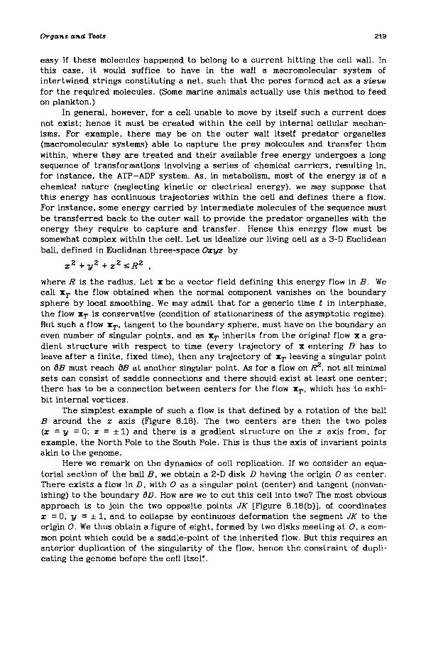
Orga",s a",ct Toots 219

easy if these molecules happened to belong to a current hitting the cell wall. Inthis case, it would suffice to have in the wall a macromolecular system ofintertwined strings constituting a net, such that the pores formed act as a sievefor the required molecules. (Some marine animals actually use this method to feedon plankton.)

In general, however, for a cell unable to move by itself such a current doesnot exist; hence it must be created within the cell by internal cellular mechan­isms. For example, there may be on the outer wall itself predator organelles(macromolecular systems) able to capture the prey molecules and transfer themwithin, where they are treated and their available free energy undergoes a longsequence of transformations involving a series of chemical carriers, resulting in,for instance, the ATP-ADP system. As, in metabolism, most of the energy is of achemical nature (neglecting kinetic or electrical energy), we may suppose thatthis energy has continuous trajectories within the cell and defines there a flow.For instance, some energy carried by intermediate molecules of the sequence mustbe transferred back to the outer wall to provide the predator organelles with theenergy they require to capture and transfer. Hence this energy flow must besomewhat complex within the cell. Let us idealize our living cell as a 3-D Euclideanball, defined in Euclidean three-space Oxyz by

x 2 + Y 2 + z 2 ~ R 2 ,

where R is the radius. Let I be a vector field defining this energy flow in B. Wecall IT the flow obtained when the normal component vanishes on the boundarysphere by local smoothing. We may admit that for a generic time t in interphase,the flow IT is conservative (condition of stationariness of the asymptotic regime).But such a flow IT_ tangent to the boundary sphere, must have on the boundary aneven number of singular points, and as IT inherits from the original flow I a gra­dient structure with respect to time (every trajectory of I entering B has toleave after a finite, fixed time), then any trajectory of IT leaving a singular pointon oB must reach aB at another singular point. As for a flow on R 2 , not all minimalsets can consist of saddle connections and there should exist at least one center:there has to be a connection between centers for the flow IT' which has to exhi­bit internal vortices.

The simplest example of such a flow is that defined by a rotation of the ballB around the z axis (Figure 8.18). The two centers are then the two poles(x = y = 0; z = ± 1) and there is a gradient structure on the z axis from, forexample, the North Pole to the South Pole. This is thus the axis of invariant pointsakin to the genome.

Here we remark on the dynamics of cell replication. If we consider an equa­torial section of the ball B, we obtain a 2-D disk D having the origin 0 as center.There exists a flow in D, with 0 as a singular point (center) and tangent (nonvan­ishing) to the boundary aD. How are we to cut this cell into two? The most obviousapproach is to join the two opposite points JK [Figure 8.18(b)], of coordinatesx =0, y =± 1, and to collapse by continuous deformation the segment JK to theorigin O. We thus obtain a figure of eight, formed by two disks meeting at 0, a com­mon point which could be a saddle-point of the inherited flow. But this requires ananterior duplication of the singularity of the flow, hence the constraint of dupli­cating the genome before the cell itself.

R. Thom

N North Pole

s

(a)

South Pole

J

K

(b)

Figure B.18 (a) Rot.ation of a ball around t.he z-axis; (b) breaking a cycle int.o t.wo re­qUires preliminary duplication of t.he cent.ral singular point.s.

How can the singularity 0 duplicate itself? Here the mathematician's goal isto replace the cybernetic execution of a program by sheer analytic continuation.The simplest approach is to consider the initial flow in D (the one of concentriccircles centered at 0) as given by the linear pencil of equation

%2 + y2 - T 2t, t = 0 .

defining the line at infinity. Now let this line at infinity approach and passthrough 0 as the axis Oy. Biologically, this means that the genome moves to theboundary wall and that the wall, extending to infinity as a straight line, mustnecessarily break (Figure 8.19). The flow is then given by the meTamorphicpotential

V = %2 + y2

2y

the flow lines of which are given by a very similar equation

%2 + y2H = - = cst

2%

Then the mirror axis Oy assumes the role of the mitotic equatorial plane and bothgenomes separate to create two distinct cells. Of course, the idea that replication

Orga:ns and: 7boLs

y

Figure 8.19 Two pencils of orthogonal circles.

)(

221

occurs through some kind of analytic continuation. where an inducer structure.being in contact with a competent medium. extends itself into a similar structureis difficult to imagine (although the centriole is not very far from achieving this).We know how life has solved the problem; it has anticipated the splitting of thegenome along Oy by replacing the single molecule 0 with a dipole system of axesparallel to Oy (note that a dipole flow is very similar to the flow defined by theHamiltonian H). By some reflection principle. this dipole creates across the mir­roring axis Oy a new dipole homologous to the preceding one, thus producing aquadrupole (Figure 8.20). Now this menage Ii quatre reorganizes as two dipoles ofaxes parallel to Ox, thus allowing the dividing line OJ: to be different from themirroring line Oy: the reader has probably recognized here the fork-like natureof the DNA semi-conservative mechanism of replication. [2] As for breaking theenvelope, this phenomenon is well known for the nuclear wall in Eukaryotes(although it occurs very posteriorly to DNA duplication). Obviously the genomehas very different structures and functions in Prokaryotes as opposed toEukaryotes.

Z22

y

R. Thom

-1

•

•+1

o

+1•

•-1

x

Figure 8.20 Quadrupole composed of two dipoles.

The Genetic Code

If we believe the metaphor that direct flux represents the dissipative energyflow of small metabolites and retroflux the polymerization of macromolecules, thenthere should be in the cell a catastrophe locus where the local regime shifts fromentraining to retroflux. It is likely that the ribosomes are those organelles inwhich such a change happens; polymerization occurs also along the DNA string, inthe synthesis of Messenger RNA. I propose that the locus of trajectories of theMessenger RNA strings, when they retreat from the DNA chain, can be consideredas a surface having the genome as boundary line (perhaps the genome in itsactivated state can be considered as an edge of regression of a singular surface:one sheet carrying the necessary precursors, the other the synthesized strings).In the spherical model B, the RNA strings move along a helicoidal surface with, asthe director curve, a spiral drawn on a cone with Oz as the axis and S (South Pole)as the vertex. In extending itself, the RNA string finally contacts ribosomeswhich, on this conical surface, are regularly situated at generator lines (Figure8.21). The conical surface can be considered as a conveyor belt bringing precur­sor material to the growing wall. Passing through the ribosomes, of course, theRNA string is translated into an amino acid chain.

The dynamics of the system may be more intelligible if we remember the toysthat children used to make when domestic heating was provided by coal stoves.The children cut from cardboard a spiraL which they attached to the top of aknitting needle stuck in a cork placed on the stove (Figure 8.22). The spiral washeld in a delicate equilibrium, its center on the top of the needle; the cardboard

Orga.ns a.nd ThoLs

String of Messenger RNA

-------

Figure 6.21 Helicoidal surface on which RNA st.rings move.

spiral comprises t.wo opposite gradients which, along wit.h its own weight and theascending hot air, cause it to rotate around the needle.

tAscending warm air

Figure 6.22 Illust.ration of t.he dynamics of Figure 6.21.

Of course, biochemists say that aU the reactions involving DNA .... RNA .... pro­teins may be realized in vitro, in the presence of the necessary precursors, ATP,ribosomes, and the relevant enzymes. This proves, perhaps, only that the enzymes

ZZ4 R. Thain

are able to direct locally the energy flow in such a way as to provide in a micro­environment the necessary energetic configuration. Anyway, the kinetics in vivoare considerably faster than in vitro.

Perhaps to understand the origin of the genetic code we should consider theribosomal reading mechanism as a modulated sieve: in a flow of amino acid precur­sors the ribosome is a funnel constructed such that the shape of the bottom holeis determined by the triplet structure of the Messenger RNA. One may well ima­gine proto-biotes living in a flow of useful molecules and able to modify the topol­ogy of the capturing sieve according to the nature of the incident molecules. Ini­tially, we can imagine that a specific molecular flow creates a puffing of a specificpart of the chromosome, leading to exploitation of this flow or triggering, by aconvenient sieve-like preprogram, a regulatory synthesis of proteins. One has toimagine a phonemic ritualization of such a process involving "puffs" only threenucleotides long. Such a number is, in fact, the least number of elements able todelineate a planar hole, the bottom of the ribosome funnel. But here, of course, weentertain yet more speculation...

Dynamics of Development in Metazoa

Here, we are interested in the embryology of triploblastic animals - ver­tebrates in particular, recalling the basic scheme expounded in Thom (1972). Thefirst differentiation splits entoderm from mesectoderm; it is interpreted as theresult of a cusp catastrophe, in which the lower regime represents the subject,the predator (entoderm), and the upper the object, the prey (ectoderm). Themesoderm's function is to capture the prey; that is, to push it to the fold point K(the mouth; Figure 8.23). This is the result of performing a hysteresis loopbetween the upper and lower regimes [pumping energy from the entodermalreserves (liver) to catch the prey]. But the presence of bilateral symmetryquickly complicates the morphology; axial mesoderms (notochords) and paraaxialmesoderms (somites) appear which split into three parts (dermatome, clerotome,and myotome) and later form vertebrae around the neural tube created by neuru­lation; and finally lateral mesoderms appear (kidneys, gonads. and the two lateralsheets, somatopheure and splanchnopleure, enclosing the coelom). The first cycle(the dorsal one) essentially develops the voluntary muscles and bones; the second(the ventral one) the involuntary muscles and vascular system (in particular, theheart).

The central theme is that the main functional hysteresis loop of Figure 8.23splits into two according to Figure B.24. A dorsal cycle involves chasing and ingest­ing the prey; a ventral cycle involves digesting the prey, storing the chemicalenergy produced by digestion, and delivering this energy to the motor organs(essentially, blood circulation). I suspect that, at least for the higher vertebratesfrom fishes to mammals, this splitting process takes place via. the budding of aloop described earlier. The fundamental hysteresis loop OAKL of the mesodermthen becomes a smooth loop [by decreasing the k coefficient of van der Pol'stheory we may produce a continuous family of concentric cycles, a conservativedynamics that is within the rectangle of the hysteresis loop, Figure B.25(a)]. Nowthe straight line t = a of the model is an internal image of the symmetry axis; itoccupies the direction v - x = cst, near to the upper left corner A [Figure

Organs and Thots

A p PreyK Mouth

Predator

Figure 8.23 Fundamental cycle of t.he mesoderm.

Head T F Food

0 .... ,A ... G Gut

Muscles M....

~I' 0 ' Digestion

Heart H L Liver (reserves)

Figure 8.24 Split.t.ing t.he mesodermal fundamental cycle into t.wo: t.he dorsal (FAMT) andvent.ral (AGLH).

8.25(b)]; the stable regime within the little triangle BAC describes the notochord(singularity of the elliptic umbilic)

V =zy (z + Y - c )

10.2In the paraaxial mesoderm (somites), the constant c vanishes, and theline v =z - z A acts as a mirroring axis for the tangent dynamics of A; thecenters of the concentric cycles are pushed towards the boundary, at the cornerA. As a result, a symmetric dynamics is formed by reflection on the symmetricangle [Figure 8.25(c)]; the centers then move away from A (as in mitosis) and thedorsal cycle is created [and also, symmetrically, the ventral cycle, Figure 8.25(d)].This describes the classic process of neural induction, where the mesodermalplate induces by contact the formation of neural tissue in the overlying ectoderm.The cell budding process occurs both in the induced ectoderm and in the inducermesoderm (but in opposite directions). In the latter tissue, after the centers havemoved away, one may obtain attracting cycles both in the dorsal and in the ventraloscillator, thus realizing a torus [Figure 8.25(d)]. A further degeneracy toward l-Dresonance may explain, by breaking the quotient circle periodically, the meta­meric splitting into somites. And by unfolding each somite along the cephalocaudal

226

A

(a)

v-x = cst

A C

o

(b)

R. Thana

(e) (d)

(e, )

Figure 8.25 (a) Continuous family of concentric cycles within the hysteresis loop;(b) the notochord; (c) axial dynamics (general); (d) paraaxial dynamics (somites);(e\) sclerotome, (ell) dermatome. (e

lll) myotome.

gradient. we may find an interpretation of the ternary splitting (sclerotome, der­matome, and myotome) arising later in somites [Figure B.25(e\-e

Il1)]. Later in the

development, the fusion of sclerotome and myotome is a suggestive image for thecanonical vertebrae [Figure 8.25(0], with the neural arch enclosing the neuraltube, and the haemal arch enclosing the dorsal aorta. The internal regimes of thesomtatopleure [Figure 8.25(h)] and the splanchopleure [Figure 8.25(i)] are purelydorsal and ventral, respectively (here the conservative character of the flowdisappears). The last regime. in its most cephalic part. keeps some oscillatorycharacter (attracting cycle) which manifests itself in the cardiac cells by elemen­tary contractions (note that the periods of this last cycle may have nothing incommon with the previously considered cycles).

To explain the intermediate development of lateral mesoderm (nephrotomes.gonads) one has to postulate that some further budding of the system of loopsoccurs. For instance, at the vertex L of the ventral rectangle (Figure 8.26. lower

Organs and ThoLs

- Haemal arch

227

(f)

(hI

(91

(i)

Figure 8.25 (cant.) (f) schema of vertebrae; (g) germinaldynamics; (h) somatopleure; and (1) splanchnopleure.

right) a new loop may be born by further budding (LKPO); LJ( represents produc­tion of waste material and OP symbolizes the external world. The edge KP is the(catastrophic) excretion of waste into the external world. The retroflux arrowsPQ and QL represent, respectively, the loss of energy due to production of wasteand the necessary injection of inorganic material (such as water and oxygen) forproducing waste material (urine, carbon dioxide). Gonads are also related to thisrepelling cycle; but the germinal line cells emanate in general from the splanchno­pleure, very near the origin A. Here again. one may conjecture that the return togerminal dynamics occurs via the straightening of the fundamental S­characteristic of the first catastrophe (ectoderm-entoderm), leading to theV = %4/4 organizing center, and then allowing the two roots emanating from zeroto develop Hopf bifurcations, in such a way as to develop for each pair of sym­metrical roots a figure of eight [Figure 8.25(g)].

Another very important budding process is the cephalic loop extending fromthe upper left vertex T into TBIS (Figure 8.26, upper left). The edge TBrepresents tracking the prey; the retroarrow IB represents the projectionemanating from the eye to the external object (the active pregnance of seeing); ISis the progressive localization of the prey, and ST its spatial localization by sen­sory inputs. This model invokes the concept that underlies the whole embryology;there is a kind of symbolic physiological blastula, the cells of which are hys­teresis loops, causally related by the identity of the same energetic flow. Thisblastula forms by successive mitoses (budding) of an original "cell" the fundamen­tal hysteresis loop of the mesoderm. As the basic physiological constraints are thesame for the whole animal kingdom, one may suspect that this physiological blas­tula is a universal structure within animal embryology (and, perhaps, also its tem­poral method of formation). But the coupling with spatial unfoldings (ill-defined,

R. Thom

0 ELIMINATION LOOP

/K

Liver /L "

0/Waste

(+Iungs) /' v (+ CO2)

Fresh /water

/of prey ~y DORSAL LOOPsensory m~ut

'" Head Foodr/ /

"-+ F" " Mouth VENTRAL LOOP

. I / Ingesting /.:J ~ ~ the prey / Gut

/ L. " G"~ /

/ I'Germinal/center L..--------f---+--...

Blood Hcirculation

M jMuscles

Lookingfor prey

'"8,Brain

Imaginary ~(being I •

the prey)

Q / pExternalworld(biodegradationof organic wastes;photosynthesis)

Figure 8.26 The physiological blastula.

both qualitatively and quantitatively) creates the variety of Ehuplans observedin nature. To take a single - striking - example, let us consider the starfish,which develops from a bilaterally symmetric larva into an organism of five-foldsymmetry. In vertebrates, the cephalocaudal axis is mapped on the vertex A ofthe physiological blastula, with a tendency to unfold along the diagonal TAL (mouthin the head, T; anus at the caudal extremity, L). When the starfish undergoesmetamorphosis, its cephalocaudal axis is spatially vertical (the mouth-anus axis);it is mapped along the ventral diagonal AL of the symbolic blastula. But the dorsaldiagonal AT (devoted to prehension activity) is mapped in the adult along the hor­izontal circle dual (perpendicular) to the central vertical axis, and it is there bro­ken into a five-order symmetry. Such huge geometrical remodelings of the bodyobviously necessitate an almost total lysis of the organic structure duringmetamorphosis.

Organs and ThoLs

Concluding Remarks

229

I hope to have shown in this chapter how the consideration of very crudeenergetic constraints, together with some genericity assumptions, may increaseour understanding of tools, organs, and embryology. Of course, orthodox scientistsmay say that such ideas are not usefuL as they do not allow experimental predic­tion or verification. To that I would like to answer that I do not claim here to pur­sue scientific data, my only aim being to revive the concept of natural philosophy.

Notes

[1] As pointed out on pp 201-211, complete vanishing of a flow is a nongeneric situa­tion. Hence It Is extremely difficult to produce preprograms that allow simultane­ous perfect opening and closing of a flow. This is why, in almost all cases, shut offfaucets do leak - a truth any owner of an apartment (or country house) can hardlydoubt. This necessary dependence of life processes on nongeneric situations suchas perfect containment has led some thinkers (e.g., J. Monod in his celebratedChance and Necessity) to appeal to contingence and randomness to explain theorigin of life. But we should not forget the constraints which control propagationsof specific physical entities; already in optics, total absence of light (full dark­ness) is relatively easy to obtain in a stable way. A solid body (a crystal forinstance) is a closed set In Euclidean space to a very good approximation. Molecu­lar biology Is undoubtedly correct to express the importance of these constraintsdue to molecular bindings, and hence to the underlying spatial geometry.

[2] In this passage from dipole to quadrupole by symmetry, the symmetry is not onlyspatial, but also internal (the symmetrical equivalent of a +1 charge Is a -1charge). In organic epigenesis such an internal symmetry cannol exist betweencells; as a result, the symmetry plane of bilateral embryos is frequently also theseparation plane of twin embryos. This appears in double-monster teratology(Siamese tWins, spina bifida, etc.). Note thal if we have In the (x; v) plane thedipole field defined by the potential V = x/ (x Z + v Z) lhen the fold map y .... xdefined by x = Y Z induces on the (y; v) plane a field defined by the meromorphicpotential

W = yZ/(y4 + v Z)

This is precisely the type of potential that occurs in our consideration of van derPol theory, pp 213-214.

References

Arnol'd, V.I. (1984) Catastrophe Theory (Berlin: Springer) translated from Russian.Dufour, J.P. (1977) Sur la si.abilit~ des diagrammes d'applicalions diff~rentiables,Ann.

Sc. Ecole Norm. Sup. (4) 10 (2): 153-74.Kergosien. Y. (1984) S~miotique de la Nature, 3e Sl!minaire de Biologie thl!orique,

(AMTB) Sol1gnac (Paris: Editions du CNRS).Lewin, K. (1951) Psychological ecology, In Field Theory in Social Sciences (New York:

Harper and Brothers) pp 174-87.SchrOdinger, E. (1957) statistical Thermodynamics (Cambridge: Cambridge Universily

Press).Thorn, R. (1972) Stabilit~structurelle et Morphogen~se(Paris: Intereditions).

230 R. Thom

Thom, R. (1963) Human psychism us animal psychism, in E. de Grolier (Ed.) Glossogenet­ics (Paris: Harwood Academic Publishers).

Waddington. C.H. (1957) The Strategy oj the Genes (London: Allen and Unwin).

This text is partly taken from a translation into English of a lecture given in French atthe StSminaire Andr~ LichntSrowicz, Coll~ge de France Paris, 1963-64, under the title Lanotion d.e programme en Biologie, to appear in Collection Interd.isciplinaire, editedby Pierre Delattre, Maloine, Paris.

CHAPTER 9

The Language of Life

David Berlinski

Introduction

In the spring of 1984, I delivered two lectures at IIASA under the title TheLanguage of Life. Dianne Goodwin was kind enough to prepare a verbatim tran­script of my talks; I have used the months since then to purge the written recordof what I said of its incoherence, vagrant inaccuracies, and general slovenliness.

This chapter is at once long and terse - an unhappy combination, and onethat makes severe demands of the reader. Many arguments are highly compressedand must be elaborated before they appear convincing. I have not hesitated tomake use of mathematical concepts in expressing myself; but I draw no mathemati­cal conclusions. I thus run the risk of alienating the general reader even as I anta­gonize the mathematician. For these reasons, it may be helpful if in this introduc­tion I endeavor to place this chapter in a somewhat wider personal and intellectualcontext.

As it stands, The Language of Life represents a draft of one-third of alarger work entitled Language, Life and Logic. Another part of that more ambi­tious project was delivered at IIASA two years ago as a set of lectures. The writtenrecord of those lectures, which I hope to publish separately as a working paper, isentitled Classification and its Discontents.

My aim in Language, Life and Logic is to explore a certain complicated com­mon ground that holds between language, on the one hand, and the graphic arts,on the other. These are the classic systems of representation of the human imagi­nation. In both, there is a curious division between the system's syntactic andsemantic structures: a theory, for example, consists of a finite set of sentences,the sentences of words; paint and then pigment comprise a painting; and yet,words and sentences, paints and pigments, manage, somehow, to cohere and, then,in a miraculous act of self-transcendence, to make contact with a distinct and dif­ferent external world. The problems of theoretical biology, it might seem, havenothing much to do with issues that arise in the philosophy of language or the phi­losophy of art. Not so. A gene comprises a linear array of nucleotides that undercertain conditions expresses a protein or set of proteins. The proteins, in turn,

232 D. BerL1.nsk1.

are organized to form a structure as complicated as a moose or a mouse. Thenucleotides are plainly alphabetic or typographic in character; the organism itselfis rich, complex, complete, continuous, unlike an alphabet. How is it, then, thatsuch typographic structures as DNA manage to express so much that is not typo­graphic at all? This is a question quite similar to questions that might be raisedabout language itself, or works of the graphic arts; and when it is pursued, certainmetaphors and quite peculiar images begin drifting from one subject to the other.There is the notion of meaning, of course, which is common to language, art, andlife; but also the idea that life is itself a language-like system; or that art isorganic. The relations of satisfaction, representation, and expression, while for­mally distinct, of course, nonetheless display points of contact. In order toexplain how it is that a painting may represent a face, for example, one hasrecourse to the notion of a metaphor, a concept from the philosophy of languageand linguistics; to make sense of gene expression, one deals in concepts such ascode, codon, information, and regulation. In a general way, a theory, a painting,and a gene belong to the class of interpreted or significant typographic objects. Itis for this reason that it has seemed to me profitable to explore some of the con­cerns of theoretical biology and the philosophy of art and language in a singlevolume.

Within the context of this chapter, my aim is to explore the ramifications ofa controlling metaphor: the idea that life comprises a language-like system. I dothis against the background of the neo-Darwinian theory of evolution - the mostglobal and comprehensive scheme of thought in theoretical biology. My argumentat its most general is constructed as a dilemma: if life is a language-like system,then certain concepts are missing from Darwinian thought; if not, then Darwinianthought is suspicious in the sense that its principles do not naturally apply to cog­nate disciplines. The intellectual pattern to this chapter is thus one of movementbetween two unyielding points, a kind of whiplash.

Part One establishes the historical and contemporary background toDarwinian thought; and makes the argument that much of biology cannot bereduced to physics. In Part Two, I consider the confluence of certain concepts:distance in the metric spaces of organisms and of strings, metric spaces in phase,complexity, simplicity, Kolmogorov complexity, the ideas of a weak theory, and alanguage-like system. Part Three plays off concepts of probability against thehypothesis that molecular biological words are high in Kolmogorov complexity ­with results that are inconclusive. In Part Four, I examine evolution or biologicalchange as a process involving paths of proteins. The discussion is set in themathematical contexts of ergodic theory and information theory. In manyrespects, the classical concepts of information and entropy are most natural indiscussing topics such as the generation of protein paths by means of stochasticdevices; but there is a connection between Kolmogorov complexity and entropy inthe sense of information theory, which remains to be explored. Almost all of PartFour represents a tentative exploration of concepts that require, and will nodoubt receive, a far fuller mathematical treatment.

Many of the points that I make in this paper I first discussed with M. P.Schutzenberger in Paris in 1979 and 1980. Indeed, it was our intention and hope topublish jointly a monograph on theoretical biology. This has not come to pass. Still,

The Language ofLife 233

to the extent that my ideas are interesting, they are his; to the extent that theyare not. they are mine.

John Casti read the penultimate draft of this essay and discovered anynumber of embarrassing errors. I am grateful for his stern advice, which I haveendeavored to heed.

PART ONE

A System of Belief

The natural thought that theoretical biology comprises a kind of intellectualLapland owes much to the idea that biology itself is somehow a derivative science,an analogue to automotive engineering or dairy management, and, in any case,devoid of those special principles that lend to the physical or chemical sciencestheir striking mahogany lustre. This is the position for which J.J.C. Smart (1963)provided a classic argument in Philosophy and Scientific Realism.[l] Analyticphilosophers, for the most part, agree that nothing in the nature of things com­pels them to learn organic chemistry; Feyerabend, Putnam, and Kuhn have won­dered whether any discipline can properly be reduced to anything at all; and,then, whether anything is ever scientific, at least in the old-fashioned and hon­orific sense of that term.[2] Naive physicists - the only kind - are all too happyto hear that among the sciences physics occupies a position of prominence denied,say, to urban affairs or agronomy. The result is reductionismfrom the top down,a crude but still violently vigorous flower in the philosophy of science. The physi­cist or philosopher, with his eye fixed on the primacy of physics, thus needs tosense in the other sciences - sociology, neurophysiology, macrame, whatever ­intimations of physics, however faint. This is easy enough in the case of biochemis­try: chemistry is physics once removed; biochemistry, physics at a double dis­tance. Doing biochemistry, the theoretician is applying merely the principles ofchemistry to living systems: like the Pope, his is a reflected radiance.

In 1831, the German chemist Uriel Wohler synthesized urea, purely anorganic compound - the chief ingredient in urine, actually - from a handful ofchemicals that he took from his stock and a revolting mixture of dried horseblood. lt was thus that organic chemistry was created: an inauspicious beginning,but important, nonetheless, if only because so many European chemists were con­vinced that the attempt to synthesize an organic compound would end inevitably infailure. The daring idea that all of life - I am quoting from James Watson's text­book (1965), The Molecular Biology of the Gene - will ultimately be understood interms of the "coordinative interaction of large and small molecules" is now a com­monplace among molecular biologists, a fixed point in the wandering system oftheir theories and beliefs. The contrary thesis, that living creatures go quitebeyond the reach of chemistry, biochemists regard with the alarmed contemptthey reserve for ideas they are prepared to dismiss but not discuss. FrancisCrick, for example, devotes fully a third of his little monograph, Of Molecules andMen, to a denunciation of vitalism almost ecclesiastical in its forthrightness and

Z34 D. Bert1.nsk1.

utter lack of detail.[3] Like other men, molecular biologists evidently derive somesatisfaction from imagining that the orthodoxy they espouse is ceaselessly underattack.

Theoretical biologists still cast their limpid and untroubled gaze over a worldorganized in its largest aspects by Darwinian concepts; and so do high-schoolinstructors in biology - hardly a group one would think much inclined to the ideaof the survival of the fittest; but unlike the theory of relativity. which Einsteinintroduced to a baffled and uncomprehending world in 1905. the Darwinian theoryof evolution has never quite achieved canonical status in contemporary thought,however much like a cold wind over water its influence may have been felt ineconomics, sociology, or political science. Curiously enough, while molecular genet­ics provides an interpretation for certain Darwinian concepts - those differencesbetween organisms that Darwin observed but could not explain - the Darwiniantheory resists reformulation in terms either of chemistry or physics. This is apoint apt to engender controversy. Woodger, Hempel, Nagel, and Quine cast reduc­tion as a logical relationship: given two theories, the first may directly bereduced to the second when a mapping of its descriptive apparatus and domain ofinterpretation allows the first to be derived from the second. I am ignoringdetails, now. The standard and, indeed, the sole example of reduction successfullyachieved involves the derivation of thermodynamics from statistical mechanics. Inrecent years, philosophers have come to regard direct reduction with some unhap­piness. There are problems in the interpretation of historical terms: theNewtonian concept of mass, for example; and theories that once seemed cut fromthe same cloth now appear alarmingly incommensurable. Kenneth Schaffner hasprovided a somewhat more elaborate account of reduction: his definition runs tofive points.[4] By a corrected theory, he means a theory logically revived to bringit into conformity with current interpretations: Newton upgraded. for example.His general scheme for reduction, then, is this:

(1) All of the terms in the corrected theory must be matched to terms in thereducing theory - a requirement of completeness.

(2) The corrected theory must be deducible from the larger theory, given theexistence of suitable reduction functions - a requirement of deriva.bility.

(3) The corrected theory must indicate why the original theory was incorrect ­a requirement of epistemological insight.

(4) The original theory must be explicable in terms of the reducing theory - arequirement of cogency.

(5) The original and corrected theories must resemble each other - a require­ment of inteUectural symmetry.

In the case of theoretical biology, to speak crisply of deriving. say. molecularbiology from biochemistry is rather like endeavoring to cut steel with butter:there is a certain innocence to the idea that molecular biology has anything like adiscernable logical structure. What one actually sees is a mass of descriptivedetail, a bewildering plethora of hypothetical mechanisms, much by way of anecdo­tal evidence. a few tiresome concepts, and an array of metaphors drawn from phy­sics, chemistry, information theory, and cybernetics. The definition of reductionjust cited is, in addition. incomplete, its flagrant inapplicability aside. In Men­delian genetics, the concept of a gene is theoretical, and genes figure in that

The Language 01 L1/e 235

theory as abstract entities. To what should they be pegged in molecular geneticsin order to reduce the first theory to the second? DNA, quite plainly, but howmuch of the stuff counts as a gene? "Just (enough) to act as a unit of function,"argues Michael Ruse, a philosopher whose commitment to prevailing orthodoxy is amodel of steadfastness.[5] The functions that he has in mind are biochemical: thecapacity to generate polypeptides; but to my way of thinking, the reductionachieved thus is illicit. In biochemistry, the notion of a unit of function is otiose,unneeded elsewhere. To the extent that molecular genetics is biochemistry, itdoes not reflect completely Mendelian genetics; to the extent that it does, it isnot biochemistry, but biochemistry beefed-up by extrinsic concepts, a conceptualpadded shoulder. What holds in a limited way for molecular genetics holds in amuch larger way for molecular biology. Concepts such as code and codon, informa­tion, complexity, replication, self-organization, stability, negative entropy(grotesque on any reckoning), transformation, regulation, feedback, and control ­the stuff required to make molecular biology work - are scarcely biochemical: thebiochemist following some placid metabolic pathway need never appeal to them.Population genetics, to pursue the argument outward toward increasing generality,is a refined and abstract version of Darwin's theory of natural selection, applieddirectly to an imaginary population of genes: selection pressures act directly onthe molecules themselves, a high wind that cuts through the flesh of life to reachits buzzing core. Has one achieved anything like a reduction of Darwinian thoughtto theories that are essentially biochemical, or even vaguely physical? Hardly.The usual Darwinian concepts of fitness and selection appear unvaryingly in place.These are ideas, it goes without saying. that do not figure in standard accounts ofbiochemistry, which very sensibly treat of valences and bonding angles, enzymesand metabolic pathways. fats and polymers - anything but fitness and naturalselection. To Schaffner's list of five, then, I would add a sixth: no Teduction bymeans of inflation - a contingent and cautionary restriction that, for the timebeing at least, enforces a stern separation between biology and mathematical phy­sics.

The Darwinian theory of evolution is the great, global organizing principle ofbiology, however much molecular biologists may occupy themselves locally indetermining nucleotide sequences, synthesizing enzymes, or cloning frogs. Thosebiologists who look forward to the withering away of biology in favor of biochemis­try and then physics are inevitably neo-Darwinians, and the fact that this theory- theiT theory - is impervious to reduction they count as an innocent incon­sistency. If mathematical physics offers a vision of reality at its most comprehen­sive, the Darwinian theor.y of evolution, like psychoanalysis, Marxism, or theCatholic Faith, comprises, instead, a system of belief. Like Hell itself, which issaid to be protected by walls that are seven miles thick, each such system looksespecially sturdy from the inside. Standing at dead center, most people have con­siderable difficulty in imagining that an outside exists at all.

The Historical Background

Charles Darwin completed his masterpiece, On the QTigin of Species, in1859. He was then forty-nine, ten years younger than the century, and not a maninclined to hasty publication. In the early 1830s, he had journeyed to the islands

Z36 D. Bert1.1l.slc1.

of the South Atlantic as a naturalist aboard H.M.S. The Beagle. The stunning diver­sity of plant and animal life that he saw there impressed him deeply. Prevailingbiological thought had held that each species is somehow fixed and unalterable.Looking backward in time along a line of dogs, it is dogs all the way. Five years inthe South Atlantic suggested otherwise to Darwin. The great shambling tortoisesof the Galapagos, surely the saddest of all sea-going creatures, and countless sub­species of the common finch, seemed to exhibit a pattern in which the spokes ofgeographic variation all radiated back to a common point of origin. The detailedsketches that Darwin made of the Galapagos Finch, which he later published in Onthe Origin of Species, show what caught his eye. Separated by only a few hun­dred miles of choppy ocean, each subspecies of the finch belongs to a single fam­ily; and yet, Darwin noted, one group of birds had developed a short, stubby beak:another, living northward, a long, pointed, rather Austrian sort of nose. The varia­tions among the finch were hardly arbitrary: birds that needed long noses gotthem. By 1837, Darwin realized that what held for the finch might hold for therest of life and this, in turn, suggested the dramatic hypothesis that far frombeing fixed and frozen. the species that now swarm over the surface of the Earthevolved from species that had come before in a continuous. phylogenetic,saxophone-like slide.

What Darwin lacked in 1837 was a theory to account for speciation, but thegreat ideas of fitness and natural selection evidently came to him before 1842, forby 1843 he had prepared a version of his vision, and committed it to print in theevent of his death. He then sat on his results in an immensely slow, self-satisfied,thoroughly constipated way until news reached him that A.R. Wallace was about tomake known his theory of evolution. Wallace, so far as I know, had never traveledto the South Atlantic, sensibly choosing, instead, to collect data in the EastIndies, and, yet, considering the same problem that had earlier vexed Darwin. hehad hit on precisely Darwin's explanation. The idea that Wallace might hog theglory was too much for the melancholic Darwin: he lumbered into print just monthsahead of his rival; but in science, as elsewhere, even seconds count.

The theory that Darwin proposed to account for biological change is a con­ceptual mechanism of only three parts. It involves, in the first instance, theobservation that living creatures vary naturally. Each dog is a member of a com­mon species and thus dog-like to the bone; but every dog is doggish in his own way:some are fast. others slow, some charming, and others bad from the first, suitableonly for crime. Darwin wrote before the mechanism of genetic transmission wasunderstood, but he inclined to the view that variations in the plant and animalkingdoms arise by chance, and are then passed downward from fathers to sons.

The biological world, Darwin observed, striking now for the second point tohis three-part explanation. is arranged so that what is needed for survival is gen­erally in short supply: food, water, space, tenure. Competition thus ensues, withevery living thing scrambling to get his share and keep it. The struggle for lifefavors those organisms whose variations give them a competitive edge. Such is thenotion of fitness. Fast feet make for fitness among the rabbits, even as a featherylayer of oiled down makes the Siberian swan a fitter foul. At any time, thosecreatures fitter than others are more likely to survive and reproduce. The win­nowing in life effected by competition Darwin termed natural selection.

The La.ngua.ge 01L'!/e 237

Working backward, Darwin argued that present forms of life, various andwonderful as they are, arose from common ancestors; working forward, that biolog­ical change, the transformation of one species to another, is the result of smallincrements that accumulate, step by inexorable step, across the generations, untilnatural selection recreates a species entirely. The Darwinian mechanism is bothrandom and determinate. Variations occur without plan or purpose - the luck ofthe draw; but Nature, like the House, is aggressive; organized to cash in on theodds.

The Central Dogma

Everthing that lives, lives just once. To pass from fathers to sons is to passfrom a copy to a copy. This is not quite immortality, even if carried on forever, butit counts for something, as every parent knows. The higher organisms reproducethemselves sexually, of course, and every copy is copied from a double template.Bacteria manage the matter alone, and so do the cells within a complex organism,which often continue to grow and reproduce after their host has perished,unaware, for a brief time, of the gloomy catastrophe taking place around them. Itis possible, I suppose, that each bacterial cell contains a tiny copy of itself, withthe copy carrying yet another copy; biologists of the early eighteenth century,irritated and baffled by the mystery of it all, actually thought of reproduction inthese terms: peering into crude, brass-rimmed microscopes, they persuaded them­selves that on the thin, stained glass, they actually saw a homunculus; the morediligent proceeded to sketch what they seemed to see. The theory that emergedhad the great virtue of being intellectually repugnant. Much more likely, at leaston the grounds of reasonableness and common sense, is the idea that the bacterialcell contains what Erwin Schroedinger called a code script - a sort of cellularsecretary organizing and recording the gross and microscopic features of the cell.Such a code script would be logically bound to double duty. As the cell divides intwo, it, too, would have to divide without remainder, doubling itself to accommodatetwo bacterial cells where formerly there was only one, Divided, and thus doubledwithout loss, each code script would require powers sufficient to organize anewthe whole of each bacterial celL The code script that Schroedinger (1945) antici­pated in his moving and remarkable book, What is Life? - he wrote in the 1940s ­turns out to be DNA, a long and sinewy molecule shaped rather like a spiral in twostrands. The strands themselves are made of stiff sugars, and stuck in the sugars,like beads in a sticky string, are certain chemical bases: adenine, cytosine, gua­nine, and thymine: A, C, T, and G, in the now universal abbreviation of biochemists,It is the alternation of these bases along the backbone of DNA that allows themolecule to store information,

One bacterial cell splits in two: each is a copy of the first. All that physicallypasses from cell to cell is a strand of DNA: the message that each generation sendsfaithfully into the future is impalpable, abstract almost, a kind of hidden humagainst the coarse wet plops of reproduction, gestation, and birth itself. JamesWatson and Francis Crick provided the correct description of the chemical struc­ture of DNA in 1952. They knew, as everyone did, that somehow the bacterial cell

238 D. BerLi7l.ski

in replication sends messages to each of its immediate descendents. They did notknow how. As it turned out, the chemical structure of DNA, once elaborated, sug­gests irresistably a mechanism both for self-replication and the transmission ofinformation. In the cell itself, strands of DNA are woven around each other andby an ingenious twist of biochemistry matched antagonistically: A with T, and Cwith G. At reproduction, the cell splits the double strand of DNA. Each half floatsfor a time, a gently waving genetic filament; chemical bonds are then repaired aseach base fastens to a new antagonist, one simply picked from the ambient brothof the cell and clung to, as in a single's bar. The process complete, there are nowtwo strands of double-stranded DNA where before there was only one.

What this account does not provide is a description of the machinery bywhich the genetic code actually organizes a pair of new cells. To the biochemist,the bacterial cell appears as a kind of small sac enclosing an actively throbbingbiochemical factory; its products are proteins chiefly - long and complexmolecules composed, in their turn, of twenty amino acids. The order and composi­tion of the amino acids along a given chain determines which protein is which. Thebacterial cell somehow contains a complete record of the right proteins, as well asthe instructions required to assemble them directly. The sense of genetic identitythat marks E. Coli as E. Coli and not some other bug must thus be expressed inthe amino acids by means of information stored in the nucleotides.

The four nucleotides, we now know, are grouped in a triplet code of 64 codonsor operating units. A particular codon is composed of three nucleotides. The aminoacids are matched to the codons: C-G-A, for example, to arginnine. In the transla­tion of genetic information from DNA to the proteins, the linear ordering of thecodons themselves serves to induce a corresponding linear ordering first onto anintermediary, messenger RNA, and then onto the amino acids themselves - this viayet another messenger, transfer RNA. The sequential arrangement of the aminoacids finally fixes the chemical configuration of the cell.

Molecular biologists often allude to the steps so described as the CentralDogma, a queer choice of words for a science.

The dour Austrian monk, Gregor Mendel, founded the science of genetics onpurely a theoretical notion of a gene, which he likened to a bead on a string. InDNA, one looks on genetics bare: the ultimate unit of genetic information is thenucleotide. All that makes for difference, and hence for charm, in the naturalworld, and which is not the product of culture, art, artifice, accident, or hardwork, all this, which is brilliantly expressed in maleable flesh, is a matter of anordering of four biochemical letters along two ropey strands of an immemorialacid.

The Central Dogma describes genetic replication; but the concepts that itscouts plainly illuminate Darwinian theory from within. Whether as the result ofradiation or chemical accident, letters in the genetic code may be scrambled; oneletter shifted for another; entire codons replaced, deleted, or altered. These aregenetic mutations: arbitrary, because unpredictable; and yet enduring, becausethey are variations in the genetic message. The theory by which Darwin proposedto account for the origin of species and the nature of biological diversity nowadmits of expression in a single English sentence. Evolution, or biological change,so the revised, the neo-Darwinian theory, runs, is the result of natural selectionworking on random mutations.

Th.e La.ngua.ge 0/L1/e

PART TWO

Evolutionary Theories

239

The popular view of evolution tends to be a tight shot on a tame subject: thedinosaur, who did not make it; the shark, who did; but the maturation of an organ­ism is itself much like the evolution of a species; only our intimate acquaintancewith its precise and unhesitating character suggests, misleadingly, I think, thatthe two processes differ in degree of freedom. Psychology, economics, urbanaffairs, anthropology, political science, and history also describe processes thatbegin in a state of satisfying and undemanding simplicity, and end later witheverything complex, unfathomable, chaotic. The contrast to physics is sobering.

The dynamics of evolutionary theories are often divided into two conceptualstages. In economics, there are macro- and micro-economic theories, aggregatedemand versus the theory of the firm; within linguistics, language at the continu­ous level of speech, and language some levels below, discrete, a matter of the con­catenation of words or morphemes. Biology, too, is double-tiered: above, the organ­ism prances; unseen, below, at a separate level, its life is organized around thealphabetic nucleotides.

Metric Spaces

By a metric space S I mean a space upon which a function

d:SxS ... R+

has been defined, assigning to each pair of points s, s' in S a nonnegative realnumber - the distance d (s, s ') - and satisfying the usual axioms:

d (s, s ') =0 <::::::;> s =s'

d(s, s') =d(s', s)

d (s, s ') + d (s " s ") 2: d (s, s ")

Double Metrics

(9.1)

(9.2)

(9.3)

The distance between organisms

The disciplines of comparative anatomy and systematic zoology classifycreatures into ever-larger sets and sets of sets: individuals (dogs, say), species,genera, families, orders, classes, phyla, taxa, and kingdoms. The classificationitself forms an algebraic lattice, with individuals acting as the system's atoms.Comparative anatomists and zoologists bring an exquisitely refined and elaborateintuition to the task of sorting the various biological creatures into appropriatecategories: the obvious cases leap to the eye; at the margins of the system, wherethe whale resides, difficult matters are decided by reference to historical andcomparative anatomy, parallel structure, common organization, biological traits,and, often, levels of biological achievement. If the image of a lattice is for the

240 D. Bert1.nsk1.

moment taken literally, then each level of the lattice, from the atoms upward,comprises a set or ensemble: of individuals, in the first instance, of sets of indivi­duals, in the second. An ensemble at any distinct level of the lattice, I assume,satisfies equations (9.1)-(9.3), and counts thus as a metric space.

The distance between strings

DNA is a string drawn from a four-letter alphabet; proteins are strings offixed length composed of 20 amino acids; as such, both strings belong to a widerfamily of string-like objects: computer programs written in a given language, thesentences of a natural language, formal systems; and acquire by osmosis a distinctconceptual and mathematical structure. It makes little difference whether stringsof DNA or strings of amino acids are taken as fundamental; and, in any case, Ioften alternate between the two. By an alphabet A I mean a fixed and finite col­lection of elementary entities called words; by the universe 0/ strings over afinite alphabet, the set of all finite sequences A * whose elements lie in A.

The natural distance between words W =w 1,,,wm , V = v 1 ... v n (W, VEA) isInl + InJ - 2 x Itl, where k is the maximum of the length of a word U = ul...Ut,

which is a subword both of Wand V. For example, let W = cadbabbd, V = xcaaba.An appropriate U is U =caab; hence D(W ,V) =8 + 6 - 2 x k.

Grantham (1974) has proposed a definition of distance in a Euclidean metricspace of proteins based on properties of composition, polarity, and volume; butthe theory of evolution suggests that changes in biological strings come aboutthrough mutations - random flash points at which letters are scrambled. Somestrings may change in a large-hearted way, with whole blocks of letters wheelingand shifting like cavalry horses; but the least mechanism to which these opera­tions may be resolved is the simple one of erasure and substitution - deletion andinsertion. The elementary processes of evolution at the molecular level lend to thenatural metric a certain simple plausibility in the face of fancy competition. T =A*, then, is a typographic metric space; dr' its natural distance.

Metric spaces in phase

M and M*, suppose, are two metric spaces; g: M -> M* assigns to each point pin M a distinct point P* in M*. M and M* are in phase under g if g acts roughlyto preserve distances: for any ~ > 0, there exists a rp > 0, such that for all p andq in M

dM(P, q) < rp -> d M- [g (P), g (q)] < ~

g is thus uniformly continuous on M; rp is, of course, a function of ~. It oftenhappens that a particular mapping between metric spaces is especially natural ­for reasons that are not mathematical. The English alphabet, for example, makesfor two metric spaces: strings of letters, sets of words. Strings of letters areclose if they agree in spelling; words if they agree in meaning. Small typographicchanges give rise to large differences in meaning: these metric spaces are not inphase. This observation is often regarded as a paradox in the context of theoreti­cal biology. In an important and influential article, King and Wilson recount evi­dence showing that chimpanzee and human polypeptide sequences are more than

The Language ofL'Ve 241

99 percent identical; the species appear further apart than a comparativeanalysis of their polypeptide chains might otherwise suggest.[6]

Complexity

Complexity and simplicity, like Yin and Yang, are metaphysical duals; exceptfor a vagrant connection to intuition, it hardly makes a difference what is calledwhich. Mathematicians and philosophers are interested in complexity for theirown ends; so are theoretical biologists, who in their better moments are quitecapable of evincing a sense of Heraclitian awe when confronted with the intrica­cies of the protozoan swim bladder. Simple counting principles often seem as ifthey might provide a general scheme for the measurement of complexity. Supposethat X is a nonempty set of objects and that A, B. C, ... are constructed from theelements of X by certain specified operations - concatenation, for example. Canwe not then say that the complexity C (x) of any object is a measure of the numberof its distinct elements and the separate and specifiable relations between them?C (x) would be a monotonically increasing function of the square of the number ofdistinct elements in any given construction. Simple, no? And intuitively satisfy­ing?

Apparently not. Label the parts of an ordinary watch in an obvious alpha­betic fashion; and the binary relations between its parts as well. The watch whenworking, let me suppose, has a complexity measured at C; but so, then, does thewatch when not working - when not assembled, in fact, binary relations being freefor the asking. Examples of this sort, when extended and made precise, suggestultimately that any complex object belongs to an embarrassingly large equivalenceclass of objects precisely equal in point of complexity.

statistical mechanical complexity

A system of identical particles moving within a fixed, bounded, and finitevolume of space constitutes a configuration; never having seen the blue smokefrom a cigar spontaneously collect in but one corner of a warm room, the thought­ful physicist - pipe, slippers, Beagle-eyes, an air of earnest confusion - concludesthat not all configurations are equally probable; yet if there are N configurationsPr(N.,) = Nt / N - this for each i. This incompatibility between what one sees andwhat one gets is known as Boltzmann's paradox, an unhappy name if only becauseno real paradox is forthcoming; but an unhappiness nonetheless. Distinct confi­gurations, Boltzmann argued, may be grouped into states; what the altogethermore elegant Gibbs called ensembles. Within thermodynamics - statisticalmechanics from above - the entropy S of a system appears perpetually in theascendancy and tends inexorably to a maximum; statistically, Boltzmann reasoned,S is thus proportional to

S=klogW; (9.4)

where k is Boltzmann's constant, and Wa measure of those configurations compati­ble with a given state - complexions as they are called in old-fashioned texts.Configurations are alike in point of probability: not so complexions; the probabil­ity of finding a mechanical system in a given state is proportional to the number of

242 D. Bertinski

distinct complexions realizing that state. At equilibrium, the complexions are at amaximum; and so, too, the entropy, which functions as a kind of ectoplasmic mea­sure of ra.ndomness or disorder.

Complexity under a classification

Statistical mechanics has a good point to its credit, and implies a second.Certain states of a physical system may be multiply realized; their number, ifcounted, makes for a measure of sorts. What is measured within statistical mechan­ics is plainly not complexity; the description of entropy as disorder serves only toexplain the whole business to the baffled undergraduate. with the explanationrapidly withdrawn by the time he enters graduate school. Still, I am struck by theextent to which the mathematical definition of entropy is made possible by anenterprising reorganization of the way in which mechanical systems are classified;in assessing complexity, a concept with a brutish family resemblance to disorder,the classification may well come first.

An example? Of course. I shall pass glowing colored slides about shortly. Con­sider the set of all functions j :Rn .... R. Those smooth functions whose criticalpoints are nondegenerate are known as Morse junctions and are at once open,dense. and locally stable in C OO(Rn , R). Any Morse function may be expressed incanonical form: if x is a critical point of j, there exists a number k such that in aneighborhood of x, and after a suitable change in coordinates,

(9.5)

Such is Morse's lemma. Their mathematical docility suggests that the Morse func­tions are simple. if anything is; but the Morse functions are simple beca.use theyare Morse functions, and not Morse functions because they are simple; simplicityis a derivative quality, like color, contingent upon a classification, and unremarkedotherwise.

The concept of a degenerate singularity makes for a simple classification onthe space of smooth functions C oo(Rn , R); but a set of objects may be simple undera classification even if the classification is itself unpleasantly complex. Writingsome years ago, Smale asked whether there exists a least Baire set V in the spaceof all dynamical systems Dyn(M) on a compact manifold M, whose elements might bequalitatively described "by discrete numerical and algebraic invariants".[7] Thequestion as posed admitted of a simple answer: no. What is needed, Smale later con­cluded, is a sequence of nested subsets Vi [Dyn(M)], where k is relatively small, Vi

open, and V k dense. As i increases, more of Dyn(M) is swallowed; as i decreases.stability and regularity properties come to the fore. It is for V 1 that Axiom A issatisfied, nonwandering sets are finite, and the transversality condition is met. V 1thus consists of "the simplest, best-behaved, nontrivial class of dynamical sys­tems "; but nothing in Smale's organization of Dyn(M) is simple at all.

A set is a.bsolutely simple under a classification if it is at once open, dense.and locally stable; under this definition simplicity does not come in degrees.Often, suitable sets turn out to be merely of the first Baire category, the best onecan do; sets that are dense need not be stable, and vice versa. First category setsand sets of measure zero coincide in the case of countable sets; but not beyond.

Th.e Language 01 L1/e Z43

From the point of view of statistical mechanics. simplicity and complexity areconcepts that involve configurations; complexity under a classification is a matterof routine: what is complex is singular. unusual. These notions may be broughtinto alignment - but only for a certain class of objects. An object A is dissectiveonly when it may be decomposed to a finite stock of parts in a finite number ofsteps. The mammalian eye is a dissective structure: so is the whole of a mouse. amoose, or a mole; but curves and concepts. the real numbers. the coast of Britain,sea-green sea-waves, and. perhaps. the entire bizarre universe of elementary par­ticles, are indissective. A dissective object is thus composed of its parts takentogether under a certain distinctive relationship. Say that A is composed of a l'

aZ..... an under R. By a relational alternative to R I mean a single permutation ofthe parts of A. If A. for example. contains but two parts. a and b. say. under therelationship R (a, b), R (b ,a) is a relational alternative to R - the only one in fact.Given R, I denote by R* the full set of all relational alternatives to R. If A isdissective it is R* that forms its complexion class: the set of all sets of its partsunder all and only their relational alternatives.

An elementary partition of a complexion class splits the class as a whole intoequivalence classes; relative to a partition. complexity and simplicity are attri­butes of equivalence classes. and are judged simply by size. To the extent that[Et ] is larger than [Ej ]. it is simpler as well; and vice versa. Almost all structuresin theoretical biology may be dissected to a finite. although very large. base; inthis sense. biological complexity and simplicity have pliant finite measures.

The mammalian eye, for example, is a dissective structure. Its parts (on onelevel of dissection, at least) are proteins, which are arranged in various delicateand precise ways. I am ignoring. now, any dynamic considerations and thinkinginstead of the mammalian eye as a static object. The complexion class to the mam­malian eye consists of all and only those rearrangements of proteins that compriserelational alternatives to the mammalian eye itself.

What makes an eye distinctively an eye, rather than some assembly of jelly­like proteins. is obviously the fact that it is capable of sight. This invocation offunction sounds an unavoidably Aristotelian note; but without some concept suchas function or purpose. theoretical biology loses much of its point. Let me parti­tion the relational alternatives to the mammalian eye into equivalence classes onthe simple basis of function. In the full complexion class, those structures thatare capable of sight fall to one side; and those that are blind and stare sight­lessly, fall to the other. Complexity and simplicity appear as matters of relativesize: the larger the equivalence class, the simpler the structures. Given the deli­cacy of the mammalian eye, most of its relational alternatives will be incapable ofsight: like the Morse functions. these complexions are simple structures; butagain, simple because they are sightless. and not sightless because they are sim­ple.

Complexity in strings

Of the 2n binary sequences of length n, some, such as

0, O. 0, 0, 0 .... (9.6)

Z44

seem simpler than others.

O. 0.1, O. 1 ....

D. BerU7Ioskt

(9.7)

for example; yet the most natural probability distribution over the space of n­place binary strings assigns to both the same probability: 2-710 . It goes against thegrain. mine. at any rate. to reckon (9.6) as likely as (9.7). especially when n islarge; but nothing in the sequences themselves indicates obviously the point ofdistinction.

The goal of science, Rene Thom has suggested. is to reduce the arbitrarinessof description; substitute data for description, and the apothegm gains my assent.A law of nature is data made compact: F =ma. said once and for all, the whole ofan observed or observable world compressed into just four symbols. A series ofobservations compactly described is rational; if rational. not random. This curiousbut compelling chain of deductions prompted Kolmogorov to argue that randomnessin binary sequences or strings migh t be measured by the degree to which suchstrings admit of a simpler description.[8] In following this line. Kolmogorov tookthe first step toward severing information theory from its unwholesome connectionto the theory of probability. If S is a binary string its length is measured in bits:an n -place binary string is n bits long. By a simpler description of S, Kolmo­gorov meant a string D shorter than S such that D describes S by acting as theinput to a fixed computer that generates S. Strings that cannot be compactlydescribed are complex, random. or information-rich; strings that can. are not;of these adjectives. only the second preserves even a vagrant connection betweenthe concept that it connotes and what is being measured. This rather inelegantidea makes plain the felt difference between a string of n Os. and a mixed string.Sequence (9.6), for example, may be expressed by a program. speaking loosely.whose length is logzn + C. If n =32, logzn =5: the relevant instruction is sim­ply to write or compute 0 25 times. C measures what little is needed to carry outthe instructions; 32 - 5 = 27, the compactness of the program. The shortest pro­gram that computes a mixed sequence such as sequence (9.7). by way of contrast.may well be close to 32 bits in length: to compute the sequence. the computer mustfirst store it precisely.

The details? They have been changing since Kolmogorov first spoke. oracle­like, on the subject in a note published in 1967; like a snake engulfing an egg. thetheory of recursive functions is engaged in swallowing algorithmic informationtheory, a development that I deplore. but accept as inevitable. Consider the set ofall n-place binary strings A* over a binary alphabet A and let TM be a fixed com­puter - a Turing machine, say; g is a general input-output function on TM map­ping strings onto strings. The compleXity of a string S of length n is the lengthof the shortest binary string D that generates Sunder TM by means of g. What­ever the complexity of S, D will plainly be maximally complex, and. hence.entirely random. Otherwise, it would not be the shortest description of S. All fin­ite length strings quite obviously have a finite measure of complexity; and only fin­itely many distinct strings of the same length have the same finite measure of com­plexity. Quite surprisingly, the decision problem for complexity is recursivelyunsolvable; this result follows almost directly from the unsolvability of the haltingproblem for Turing machines. Like truth, randomness is a property that remainsineluctably resistant to recursive specification.

The La.l1.gua.ge 01L1/e 245

If all else fails. a binary sequence of length n may be generated by a binarysequence of length n: there are 2l1. such algorithms. and 2l1. -1 - 2 algorithmsshorter than this. On any reasonable interpretation of complexity. algorithmswithin a fixed integer k of n itself must be reckoned random or complex or nearlyso. Thus 2l1. -k -t - 2/2l1. algorithms have a complexity less than n - k; and arehence nonrandom or simple. If k = 10. this ratio is roughly 1 in 1000; of 1000binary sequences of length n. only one can be compressed into a program morethan ten bits shorter than itself. Hence:

Theorem 9.1 The set of random sequences of length n in the space A* of allbinary sequences of length n is generic in A * .

These random sequences are simple under a classification because they are typi­cal, but complex in a stronger and more absolute sense because they are randomor information-rich. In this context. genericity is a finite measure of size. Thenumber of purely random strings grows exponentially with n. of course. If mostbinary sequences are random. the appearance of sequence (9.6) prompts a naturalstochastic surprise: sequences such as (9.7) are what one expects. The definitionof Kolmogorov complexity may be directly extended to recursively enumerablesets; sets of strings especially, and hence languages.

Language-like Systems

When it comes to language. there is syntax and semantics. Phonetics is theprovince of the specialist; pragmatics remains a pale albino dwarf. To semanticsbelongs the concept of meaning; to syntax. the concept of a well-formed formula ora grammatical sentence. The reference to logic is happy if only because ithighlights the fact that language-like systems go beyond the natural languages.Any language no doubt exists primarily to convey meaning: but meaning inmathematics is a matter of a model - an extrinsic object.

The construction of strings within a language-like system involves con­catenating or associating simpler strings; any finite string may be dissected to afinite set of least elements. Going up. concatenation: going down, finite dissection;retrograde motion of this sort suggests that language-like systems on this level berepresented algebraically as semigroups. Let A be any nonempty set of objects ­words. for example. or letters, or numbers. A has the structure of a semigroup ifthere exists a mapping A x A .... A such that for all a. b, and c in A

(aob)oc = ao(boc) .

In English words go over to sentences from left to right; in Hebrew. from right toleft; but in any case, one step at a time. Let A be a finite set of words now. withwords understood implicitly as the least elements of a natural language: and let A*be the set of all finite sequences (a 1 .... ,al1.) whose elements !al, ... ,al1.~ lie in A.To endow A* with the structure of a semigroup. it suffices to define an associativemapping A* x A* .... A* : easy enough. If

8 1 = (al ... ·. am)

246

and

then

8 1 0 8 2 = (c1'···. cm +7I.) •

where

C1. = a1.; c m +j = b j •

i =1. 2, ...• m; j =1. 2 ..... n

D. BerL1.7I.sk1.

A* is at once a free-semigroup over a finite alphabet and a universal language:no sequences are left out.

Almost all language-like systems are large in the sense that they have manydistinct strings. Meditating on the matter in the late 1950s. and regularlythereafter. Noam Chomsky argued that every natural language is infinite by virtueof its recursive mechanisms - conjunction and alternation. for example - and.simultaneously. that such mechanisms are recursive by virtue of the fact thatevery natural language is infinite. Both halves to this argument. taken together.describe a closed circle in space. Whatever the truth, language-like systems. ifthey are infinite, are countably infinite and no bigger.[9]

Going further toward a definition of a language-like system involves the bad­lands beyond triviality. Linguistics. the French linguist Maurice Gross once provo­catively remarked. admits of but a single class of crucial experiments. Nativespeakers of a given language are able to determine whether a given sentence isgrammatical. Experiments of this sort exist because no language-like systemencompasses the whole of a set of strings drawn on a finite alphabet - a curiousand interesting fa.et, which the sheer concept of communication might otherwisenot suggest. The distinction between grammatical and ungrammatical stringsinduces a primitive classification on a language-like system; and reflects an evenstronger principle of fastidiousness: the vast majority of language-like strings arenot grammatical at all and represent syntactic gibberish. The fastidiousness oflanguage-like systems is yet again a fact: it would be easy. if unrewarding, todesign an artificial language in which most strings were grammatical. From thepoint of view of grammar. the strings of a natural language are complex under theclassification of strings into grammatical and ungrammatical sets. With the stringsarrayed in front of the mind's bleak and rheumy eye. in ascending order. bylength, with sets of strings stacked like an inverted pyramid. the grammaticalstrings in a language-like system appear as nothing more than a thin smudge; theyare thus complex under this classification because they are singular. unusual.The origins of this bit of natural history are to be discovered. no doubt, in thealgorithmic properties of the human brain: in order to store a natural language.the brain must first represent it - in the form of recursive rules. for example.This suggests that language-like systems are low in point of Kolmogorov complex­ity; and from this point of view, simple.

A natural language. I have already observed. realizes two metric spaces (cf. p240); but the informal example that I gave involved the concept of meaning, and

The La:n.gua.ge ofL1,fe Z47

not grammar. No matter: the point carries over to the case at hand - andcomprises the third of three queer natural facts that nothing in the concepts ofgrammar or communication obviously implies. Thus, let T be a typographic metricspace of strings under the natural metric; the same set of strings comprises asecond metric space under the degenerate distance function d*: if sand s' areboth grammatical. d* (s . s ') = 0; if not, d* (s . s ') = 00. These are the natural and(degenerate) grammatical metric spaces of a language-like system. In a language­like system, natural and grammatical metric spaces are plainly not in phase.

Two models or generation

Linguistics is a rebarbative, hair shirt of a subject; and grammar a vexingproperty. Linguists, for reasons of their own. are often interested in the weakestof generative devices that specify all and only the sentences of a naturallanguage.

Representation by grammar

A phrase structure grammar is a quadruple G = (A,T,S.P). where A issome finite alphabet of symbols: T. a distinguished subset of A - the set of so­called terminal symbols; S, a distinguished initial symbol; and P. a finite set ofproduction rules of the form u ..... 'IJ; U is a nonempty set of nonterminal symbols,and 'IJ some specified string of characters. The set of all strings of terminal sym­bols constitutes a phrase structure language - a proper subset of the set of allstrings A* defined over A.

By a context-free production rule. I mean one in which u may occur in anycontext - in effect, a rule in which u figures in isolation. Correspondingly, thereare context-free grammars.

Example 9.1 Let A = (a, b), T = (a ,b), and P be the two rules S ..... ab; S ..... a..Sb.This grammar generates all and only the strings of the form a nb n.

Representation by systems 0/ equations

Consider the context-free grammar G whose production rules are S ..... a..Sl:1 •and S ..... c, where T = (a, c), and S is an initial symbol. Let the variable / t rangeover terminal symbols. The action of the production rules may be mimicked by anequation:

S =/1 +/z+ ... +/n .

where addition is construed as set theoretic union. For G,

S=aSa +c.

Replacing S by SO = c ,

S (1) = aca + c .

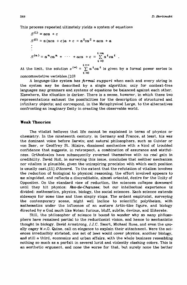
248

This process repeated ultimately yields a system of equations

S(1) =aea + e

S(2) =a (aea + e)a + e =a 2ea 2 + aea + a

t =nS(n) =anea n + ... + aea + e = L: atea t

t=O

D. Berttnskt

t=ooAt the limit. the solution s(oo) = L: a tea t is given by a formal power series in

t=Ononcommutative variables.[lO]

A language-like system has formal support when each and every string inthe system may be described by a single algorithm; only for context-freelanguages may grammars and systems of equations be balanced against each other.Elsewhere, the situation is darker. There is a sense. however, in which these tworepresentations exhaust the possibilities for the description of structured andinfinitary objects; and correspond, in the Metaphysical Large, to the alternativesconfronting an imaginary Deity in creating the observable world.

Weak Theories

The vitalist believes that life cannot be explained in terms of physics orchemistry. In the nineteenth century, in Germany and France, at least. his wasthe dominant voice before Darwin; and natural philosophers. such as Cuivier orvon Baer, or Geoffrey st. Hilaire. dismissed mechanism with a kind of troubledconfidence that suggests, in retrospect. a combination of assurance and wistful­ness. Orthodoxies have subsequently reversed themselves with no real gain incredibility. David Hull, in surveying this issue, concludes that neither mechanismnor vitalism is plausible. given the uninspiring precision with which each positionis usually cast.[ll] D'Aeeord. To the extent that the refutation of vitalism involvesthe reduction of biological to physical reasoning, the effort involved appears tome misguided. and reflects a discreditable. almost oriental, desire for the Unity ofOpposites. On the standard view of reduction. the sciences collapse downwarduntil they hit physics: Rez-de-Chausee; but our intellectual experience isdivided: mathematics. physics. biology, the social sciences. Each science extendssideways for some time and then simply stops. The ardent empiricist. surveyingthe contemporary scene. might well incline to scientific polytheism. withmathematics under the influence of an austere Artin-like figure. and biologydirected by a God much like Wotan: furious, bluff. subtle. devious. and illiterate.

Still, the philosopher of science is bound to wonder why so many philoso­phers have remained partial to the reductionist vision, and hence to mechanisticthought in biology. David Armstrong, J.J.C. Smart, Michael Ruse. and even the usu­ally cagey W.v.O. Quine, call on elegance to explain their attachment. Were the sci­ences irreducibly striated, one set of laws would cover physics. another biology.and still a third, economics and urban affairs. with the whole business resemblingnothing so much as a parfait in several lurid and violently clashing colors. This isan aesthetic argument, and none the worse for that. but surely none the better

The La:ngua.ge 01Life 249

either. If elegance is inadequate as a motive, intellectual anxiety, realized uncons­ciously, is not.

Vitalism commences from the conviction that nothing in our experience ismuch like the life that ripples and bubbles so abundantly over an entire planet,and nowhere else, apparently. Now mathematical physics is not only the pre­eminent discipline of our time - it is where the laws are. Evolutionary theories inbiology are weak in the sense that they are not directly sustained by the author­ity of physics; and, worse, weaker still in being counterphysical. Thermodynamicarguments count against the very existence of the structures that they are meantto explain. Fact heavy, law poor, such theories remain surprisingly resistant toconfirmation. Were biology an aspect merely of physics, the sceptic would getshort shrift: there, the answer to whether what works, works, is simply that itdoes.

Science is unavoidably general. To say that copper conducts electricity isweakly to imply the counterfactual conditional that were anything much likecopper it would conduct electricity as well. It has often appeared to philosophersof science that specifying what it means for something - an :c, say - to be muchlike copper inevitably comes to claiming that, among other things, :c conductselectricity. Still, the similarity in structure between two domains of discourse ­computer programs and natural languages, for example - may be obvious ongrounds other than the fact that they share the same laws.

When I speak of a theory, I follow the logician's lead: a theory consists of aconsistent set of sentences in a given language; the set-theoretic or algebraicstructures in which a theory is satisfied comprise its models. Two models thatshare the same structure are isomorphic and hence elementarily equivalent in thesense that they satisfy the same sets of sentences. What I am after is a weakernotion entirely - partial similarity in structure. I know of no way, unfortunately,to define this concept so that the definition applies equably to biology, and, say,geology; I suspect, in fact, that partial similarity in structure will require a defini­tion with indefinitely many separate clauses. Whatever the details, similarity instructure is bound to be a matter of degree, so that it makes sense of sorts to sayof two models that they are at a certain distance, one from the other. In this waya family fM1.l. i = 1, 2 .... of (possibly) first-order models may be given an appropri­ate and empirical metric structure.

Suppose that T is a theory holding in M; and let M* be a model at some fixeddistance from M. By the symmetric difference T I T* of T I mean the number offormulas T* of T that fail to hold in M* when T is interpreted in M*.

A theory T is general, I shall say. if for any e > 0, there exists a 6 >a (afunction of e, of course) such that

d(M,M*) < 0 .... TIT* < e (9.8)

Generality in my sense is a kind of stability; and as Dr Johnson remarks, thesoul must ultimately repose in the stability of the truth.

To see an analogy between the operations of life, on the one hand, and theoperations of language, on the other, is to raise the question whether the laws ofbiology have a natural and legitimate interpretation in linguistic terms. I am myselfindifferent to the fate of the Darwinian theory, and perfectly prepared tobelieve, along with Wickramasinghe and the luckless Hoyle, that life originated inouter space, or that the Universe-as-a-Whole is alive and breathing stertorously;

250 D. Berti1l.ski

but if Darwinian theories work in life, they should work elsewhere - in language­like systems, I should think. Should they fail there, this may be taken as evidencefor the inadequacy of Darwinian theories, or as evidence for the inadequacy of theanalogy that prompted the comparison in the first place.

I stress this point if only because it has so often been misunderstood.

Life as a language-like system

It was von Neumann who gave to the idea that life is like language a part of itscurious current cachet. The last years of his life he devoted to a vast and clumsyorchestration of cellular automata. showing in a partial fashion that when properlyprogrammed they could, like abstract elephants, reproduce themselves. Someyears before, McCulloch and Pitts had constructed a series of neural nets in orderto simulate simple reflex action; Kleene demonstrated that their nets had thepower of finite automata and were capable of realizing the class of regular events;von Neumann's automata had the full power of Turing machines. Michael Arbib, E.F.Codd. G.T. Herman, A. Lindenmayer, and many others, have carried this work for­ward, with results that asymptotically approach utter irrelevance.[12] Yet theanalogy between living systems and living languages has not lost any of its brassycharm. There is information, of course, which is apparently what the genes store;replication, coding; messages abound in the bacterial cell, with E. Coli, in particu­lar. busy as a telephone switchboard. So striking has the appropriation of termi­nology become, that some biologists now see the processes of life, in all their gran­deur, as the effort of a badly protected and vulnerable bit of genetic material tokeep talking for all eternity.

Unlike an argument, an analogy stands or falls in point of plausibility; goodarguments in favor of bad analogies are infinitely less persuasive than bad argu­ments in favor of good analogies. Certainly the proteins, to stick with one class ofchemicals, may be decomposed to a finite base - the 20 amino acids. The precise,delicate, dance-like steps that are involved in their formation suggest, moreover,that they satisfy some operation as abstract as concatenation. On the other hand,the number of possible proteins, although large, is finite; but one of the joys ofanalogical reasoning is the vagueness with which the line between success orfailure may be drawn.

The grammatical strings of a language-like system are low in Kolmogorov com­plexity, and so are not random. Such is the fastidiousness of a language-like sys­tem. What of the proteins? If they are random, it makes little sense to think ofthem as biological words or sentences. Jacques Monod, whose metaphysical attitudetoward biology suggested nothing so much as a kind of chirpy bleakness, drewattention to the random character of the proteins in 12 hasa.rd. et la. necessite;his argument has been gravely accepted by many molecular biologists.[13] In fact,the evidence leading to his conclusion is fragmentary; the standards of random­ness to which he appealed, imprecise. Thus it struck Monod that knowing, say, 249amino acid residues in a chain 250 residues in length, one could yet not predictthe last member of the chain; much the same is true for English sentences, ofcourse; it is, in any case, simply untrue that protein strands exhibit such wantondegrees of freedom. Within protein chemistry, there are many instances of whatappear to be strong internal regularities: palindromic patterns, for example.

The Lmngumge 0/L'/,fe Z51

Nonetheless, I am in sympathy with Monod to this extent: it is unlikely that theanalogy between life and language will be profitably pursued on the atomistic levelof the nucleic acids or the proteins themselves.

PART THREE

Arguments Good and Bad

The theory of evolution is haunted by an image and an observation: the first,that of the hapless chimpanzee, typewriter-bound, endeavoring, quite by chance,to strike off the first twenty lines of Hamlet's soliloquy: the second, the commentof an anonymous Jansenist logician, who remarked, quite sensibly, "that it wouldbe sheer folly to bet even ten coppers against 10000 gold pieces that a childarranging at random a printer's supply of letters would compose the first twentylines of Virgil's Aneid". Image and observation do not quite cohere into a singleargument: it is clear in neither case how the imagined stochastic experiment is tostop. Still, the notion of randomness yet lies at the center of evolutionarythought, and there it sits, toad-like and croaking. On the simplest and most intui­tive conception of probability, what can occur is weighted against the backgroundof what might occur: five diamonds: all other combinations of the cards. In poker,there are 2598960 five-card hands, but only 5148 flushes. It is their ratio thatone might expect to observe as cards are actually dealt; but in the longest of longruns, the passage to the limit gives content to the intuitive idea that a number ofsuccessive trials will converge to a particular real number: 0.002, for example, ifflushes are being counted.

One of the curiosities of the very notion of probability is the inescapabilityof the improbable. The laws of thermodynamics, to take a notorious example, areanisotropic: they go in one direction; downhill, as it happens, a circumstance withwhat appears to be overwhelming personal support. Statistical mechanics providesa brilliant and persuasive explanation for thermodynamic laws; yet Poincar~

demonstrated, in an absurdly easy proof, that any statistical mechanical confi­guration, of whatever degree of implausibility - k molecules of gas, for example,occupying 1/V of the total volume V of a finite and bounded container - is boundto recur, in all its vividness, poignant symmetry, and complexity, given enoughtime. Physicists often explain the discrepancy between thermodynamics and sta­tistical mechanics by arguing that the time involved is very long. No doubt.

The evolution of life on this planet is, as Darwin realized, not a hurriedaffair. Early on, Darwinian biologists got rid of the theological limits set to the ageof the Earth by Bishop Ussher and others in the seventeenth century; the scalewithin which Darwinian evolution might have worked is bounded by perhaps fivebillion years. Nineteenth century biologists assumed that whatever else one mightsay about Darwinian biology, it would not fail for lack of time; this thesis twentiethcentury biologists have carried over intact.

Five billion years is apt to seem long if one is counting the minutes; but it isnot long enough to sample on a point by point basis a space whose cardinality isroughly 1015 - touching base with a new point at every second, say; and yet thereare 20250 possible proteins - a number larger by far than the expected life of the

D. Berttnskt

universe measured in seconds. In a space of this size, the odds against discover­ing a specific protein - fishing it from an urn, say - are prohibitive: 1 in 20Z50.

I spoke hastily just now of a specific protein: if a.ny protein will do. the oddsimprove: in a uniform probability space tat l. Pr(al v a 2 '" v at} =1. The dis­tinguished British biologist Peter Medawar has seized upon this point, and com­menced happily to trot, but in what I think is the wrong direction.[14] "Biolo­gists," he writes, "in certain moods are apt to say that organisms are madlyimprobable objects or that evolution is a device for generating high degrees ofimprobability. I am uneasy about this entire line of thought," he continues, "forthe following reason:

Everyone will concede that in the games of whist or bridge anyone particularhand is Just as unlikely to turn up as any other. If I pick up and inspect a par­ticular hand and then declare myself utterly amazed that such a hand shouldhave been dealt to me, considering the fantastic odds against it, I should betold by those who have steeped themselves in mathematical reasoning that itsprobability cannot be measured retrospectively, but only against a priorexpectation ... For much the same reason, it seems to me profitless to speakof natural selection's 'generating improbability' ... it is silly to be thunder­struck by the evolution of organ A if we should have been Just as thunder­struck by a turn of events that had led to the evolution of B or C instead."

Medawar is roughly right about probability: the fallacy to which he refers isthe error of retrospective specification; and consists precisely in reading backinto an original sample space information revealed only on the realization of a par­ticular event. In poker, a deal distributes n hands of equal probability: 1 in2598960, as it happens. This sample space is retrospectively specified if one handin particular is contrasted with the full set of 2598959 hands that remain, andprobabilities assigned to the partition so created; what appears initially as oneamong equiprobable events becomes under retrospective specification an improb­able event in a sample space of only two points. It is embarrassing for an author topoint such things out. Still, Medawar is wrong in the general conclusions that hedraws from this paragraph. Card sharps and statisticians are little interested inthe set of all five-card sequences. In poker, sequences are initially partitionedinto equivalence classes of uneven size: a royal straight flush, of which there arefour, a straight flush, four of a kind, a full house, a straight, three of a kind. twopairs, and, then, finally, whatever is left - the vast majority. There are four waysto achieve a royal straight flush; many more ways in which to realize a full house.Since they are specified in advance, partitions in poker carry no taint of retro­spection; and plainly, in poker there is only a rough correlation between theinternal character of sequences within a partition and their payoffs: what isimportant here, as elsewhere, is the classification, which is very largely arbi­trary.

Medawar's argument, on its face, thus involves rather an uninspiring mistake,but it is not yet a mistake in evolutionary thought. The human eye, a chastenedMedawar might argue. turning his back on his own analogy between life and thecards, represents one arrangement of its constituents: any other might have doneas well. In admiring the structure that results, we suffer from misplaced awe, likea toad contemplating a dog. Does this argument carry conviction eye-wise? Is itreasonable to suppose that any other arrangement of the eye's constituents wouldresult in an eye? In anything at all? The question sounds an unavoidably Aristo-

Th.e Language 01 Life 253

telian note: an eye is an organ with a specific function - sight, most obviously; aneye-like configuration does not count as an eye unless it can see. To frame thediscussion thus is to answer the question immediately, at least on the level ofintuition; but what I have said must not be confused with an argument in refuta­tion.

Vmble proteins

Linguistics is possible if only because human beings have strong and reliableintuitions about natural languages. The polypeptides are alien strings, accessibleonly through an arduous act of the biochemical imagination. Grammar effects asegregation of strings in a language-like system; beyond grammar, aloof, untouch­able, there is meaning; the two concepts do not coincide. Some grammaticalstrings, in a natural language, at least, are grammatical and meaningless; others,meaningful but ungrammatical; but meaning and grammar belong together, yokedpairs in the same corner of some dimly understood conceptual space. An algebraicsystem of strings in which no distinctions of meaning and grammar are recognizedis profligate; and pointless because of its profligacy.

In a preanalytic sense, the concept of meaning indicates a kind of coherence;and has a usefulness of application in domains other than language. A life weLL­spent is meaningful: its parts and patterns are ordered; fuLL with life, biologicalcreatures are filled with meaning, a kind of blunt, irrefrangible purpose; in death,this meaning disappears, and what is left, the corpse and its grim constituents,appears aLL at once to lose the integrity of the creature itself, and becomes,instead, a thing among other things, an object merely. To the vitalist, livingcreatures instantiate some unique property that remains stubbornly unseen else­where - in the domain of objects studied by mathematical physics, for example; indeath, this property vanishes, Like a fluid evaporating. In mechanistic thought,the passage from Life to death is rather like a phase transition, a singularity ofsorts in the trajectory of the organism, a disabling and permanent catastrophe,that reflects, as it must, only a change in the constituents of the organism, a vari­ation in its underlying pattern. The concept of a complexion, whichfigures in statistical mechanics, provides a useful measure of meaning. The com­plexion set to a biological organism represents those relational alternatives of itsbiological parts that correspond to living systems. The unalterable fact that livingsystems die and hence do not persist indicates that some of their complexions failto preserve life and hence meaning; in fact, the number of meaningless complex­ions must be significant: most of the arbitrary rearrangements of a complex organ- a mammal, say - result in nothing more than a botch - a circumstance withwhich every surgeon is familiar. The Central Dogma of molecular biology estab­lishes a relationship between strings of nucleotides and strings of proteins; to theextent that the whole of a biological organism may be resolved into its protein-likeparts, the Central Dogma establishes a larger, more indirect, relationship betweenmolecular biological order and order in the larger sense of life. This relationshiphas an inverse: if only certain forms of life have meaning, this, too, is reflected, asit must be, in the universe of molecular biological strings - on the level of stringensembles, for example. If certain protein ensembles are meaningful, and not oth­ers, this suggests, but does not imply, that the same distinction is palpable on thelevel of the individual proteins themselves. The term viable I mean as a biological

D. Bert1.nsk1.

coordinate to the Siamese concepts of meaning and grammar; a protein is viableonly when it achieves a certain minimum level of biological organization and useful­ness. What level? What kind of organization? Usefulness in what respect and towhat degree? Who knows?

F'ullloads, fair loads, fair samples

In a natural language, sentences decompose to words; words to letters. Gram­matical constraints hold weakly at the level of English words. The set of all word­like combinations of English letters of fixed length n, I shall say, make up a fullload; the set of all grammatical words, a fair Load. Within molecular biology, a fullload corresponds to all possible proteins of normal length: a set whose cardinalityis 2025°. To the fair loads in English correspond the viable proteins in molecularbiology. How large is the biological fair load? Again, who knows? Whatever its ulti­mate size, those proteins that have already been synthesized in the course of bio­logical history are viable if anything is: nothing succeeds like success. This set isa fair sample of a fair load. Its size Murray Eden calculates at 2052 . The taskthat he sets himself is the infinitely delicate one of drawing inferences about thefair load from its fair sample.[15]

Between the fair sample of a fair load, and the fair load itself, is the differ­ence between what is and what might be; between the fair load and the full load,the difference between biology and mathematics. In English, the differencebetween the fair load and the full load is as absolute as death. Any two words ofEnglish thus resemble each other more than they are likely to resemble a wordgenerated at random from the letters of the English alphabet. In the case of thepolypeptides, Murray Eden writes:

Two hypot.heses suggest. t.hemselves. Eit.her funct.1onally useful prot.eins arevery common t.o t.his space, so t.hat. almost. any polypept.1de one is likely t.o findhas a useful funct.1on t.o perform, or else t.he t.opology appropriat.e t.o t.hisprot.ein space is an import.ant. feat.ure of t.he explorat.1on: t.hat. is, t.here exist.scertain st.rong regularit.1es for finding pat.hs t.hrough t.his space.

In asking whether the viable proteins are common in the space of all polypep­tides, Eden is asking, in effect, whether the fair sample is marked by discernablestatistical regularities. "We cannot now discard the first hypothesis," he adds,"but there is certain evidence which seems to be against it: if all polypeptidechains were useful proteins, we would expect that existing proteins would exhibitvery different distributions of amino acids." Statistical tests appear to show thatpairs of proteins are drawn from a common stock. His example involves the alphaand beta human hemoglobin chain. One form of hemoglobin has 146 amino acid resi­dues, the other 140. The two chains may be set down, side by side, and matched,residue by residue. They agree at 61 points; there are 76 points at which theydiffer, and 9 points at which no match is possible because the chains are not ofthe same length. It is plausible that one chain was derived from the other, or thatboth were derived from a common ancestor. What is curious about these pairs ofproteins, however, is the fact that even though the chains do not agree completelYin the order of their amino acids, they do agree in their distribution; reasonenough, Eden argues, to suppose that the proteins themselves are drawn from astatistically significant fair sample.

The criticism of this historically important argument, I leave as an exercise.

(9.11)

The La.n.gua.ge 01Li/e

Delicate inferences

In What is Li,fe?, Schroedinger argued that living systems must haverecourse to what he dubbed an "aperiodic crystal" in order to store information.Crystals are repetitive, regular, and information poor; the order of a living systemis specific. irregular. information rich. There is a certain splendid effulgence tothe vocabulary of theoretical biology that it would be uncharitable not to cherish.H.P. Yockey identifies order with Kolmogorov complexity; and so does R.M. Thomp­son, a mathematician who in writing on theoretical biology alternates betweeninformation theory and a pious endeavor to communicate to the reader his appre­ciation for the many faces of Krishna.[16] On the other hand, G.J. Chaitin andR.M. Bennett identify biological order with algorithmic simplicity. A division ofintuition on so fundamental a point may suggest a degree of conceptual confusionapproaching the schizophrenic.

If biological words are characterized by a high degree of Kolmogorov com­plexity, could time and chance have combined to discover a structure comparable,say. to cytochrome c or any of the modern hemoglobin chains? This is the ques­tion raised by the redoubtable H.P. Yockey: the problem as posed has but twoparameters.[17] In the beginning the primeval soup, which I always imagine asrather a viscous, Borscht-like fluid, contained perhaps 1044 amino acid molecules.There is, inevitably, an element of fantasy to all quantitative calculations of thissort. At each second, over the course of 1 x 109 years, an indefatigable stochasticDeity arranges and then rearranges the 1044 amino acid residues in sequenceswhose length N = 101. There are

20101 or 2.535 x 10131 (9.9)

such sequences. The odds against discovering anyone in particular thus stand at 1in 2.535 x 10131. Not all residues, however, are equally probable. Save for a verylarge set of strings of small probability, the number of sequences of length N is

a NH (9.10)

where

n.H =- L PJ loga PJ

J =1

Here PJ measures the probability of the jth residue, and a = 2, so that H ismeasured in bits.

In the end - the details are not important to my argument - Yockey con­cludes that

H =4.153 bitsl residue

the number of 101 place sequences is

24 .153 )(101 =1.6067 X 10126 .

(9.12)

(9.13)

"Information theory," he remarks, "shows that, in this case, the actual number ofsequences is smaller than the total possible number by a factor of 105 ". Now thereare, in all, 3.6 x 1061 families of cytochrome c sequences; in order to obtain anyone of them by chance, Yockey argues, it would be necessary to repeat an elemen­tary stochastic experiment 3.15 x 1058 times on 108 separate planets "in order to

D. BerLind:i

have a reasonable expectation of selecting at least once a member of the ensembleof 3.8 x 1061 cytochrome c sequences in only ten of them".

From nothing, nothing, the Darwinian doubters have always claimed; and Ihave been there with the best of them; but this argument, couched as it is largelywithin the algorithmic theory of complexity stands on what seems to me dubiousground:

(1) A binary string is random to the extent that its shortest program is roughlyof the same length as the string itself; this definition trades only in countingbits. Now, the impulse to assert that contemporary proteins are random owesmuch, I think, to the rather primitive idea that life, if complex, requires com­plex constituents or atoms; I have suggested something similar in arguing thatthe proteins inherit a grammatical distinction from the structures that theyconstitute. Kolmogorov complexity, however, is ill-defined on any level of bio­logical organization past the molecular; but even if a mammal or a molluskcould be represented as a binary string, nothing suggests that those stringswould be high in Kolmogorov complexity. Quite the contrary. Life in the large,on the level of the organism itself, is organized with what appears to be briskalgorithmic efficiency. Living creatures are simple in the sense of Kolmogorovcomplexity; but complex under the classification of their complexions. In thissense, they behave much as a language-like system. This observation is com­patible with the thesis that protein strings are, nonetheless. high in Kolmo­gorov complexity; but it is compatible, too, with the contrary thesis that pro­tein strings reflect the complexity of life by means of their organizationand not their complexity. Nothing in the concept of Kolmogorov complexitymeasures the algorithmic organization of a string or set of strings; twoequally complex strings may well differ in their time complexity to theextent that only one is polynomially bounded.

(2) The difference between the space of available proteins, and the small subsetactually chosen by evolution, makes for a trite contrast; yet what lends tocytochrome c its position of statistical distinction? "Because of the very fun­damental function of the cytochromes," Yockey writes, " ... the histones andother proteins, which are believed to be of very ancient and even pre­cellular origin, one cannot relax the specificity requirement derived fromcytochrome c" [emphasis added]. In generous conversation, Yockey has ampli­fied this point by suggesting that the specific protein chains necessary forlife correspond to the set of words in a language - fair and not full loads; acurious remark inasmuch as words in a natural language are low, and not high,in Kolmogorov complexity. Still, I am sympathetic to the drift of this line; butthe difficulty goes beyond the problems of an imperfect analogy. Certainclasses of proteins. Yockey argues, are necessary for life. Such are theinformation-rich, complex strands; other strands are specific in the limitedsense that they are statistically unlikely: "only a tiny fraction of the (avail­able) sequences will carry specificity." It follows by Theorem 9.1 (p 245)that specificity and complexity are not the same thing: the set of complexstrands (of a given length) is in the majority; their emergence is probabilisti­cally favorable, indeed, unavoidable. Cytochrome c, considered simply as acomplex protein. is no more likely to appear than any other complex protein;but no less likely either. Having discovered cytochrome c, quite by chance,

Th.e Language 01L1,fe 257

Life might have made do with any other protein of comparable complexity. Ifby specificity. Yockey means statistical unlikelihood in a uniform samplespace - the space of all complex proteins. for example - his surprise at theemergence of cytochrome c is attributable to retrospective specification; ifnot. what then is specificity. the mysterious middle term to his argument? Ifthe specific proteins have some independent description. Yockey does notprovide it; and their size. apart from suggesting that it is low. he does notcalculate.

PART FOUR

Der Prozess

The evidence in favor of the thesis that proteins are random sequences ofamino acids is exiguous; and random words may well be grouped into nonrandomsequences. This suggests that the close study of the statistical properties of cer­tain proteins may involve a kind of dense conceptual myopia. something thatreflects a passionate absorption in minutiae. The process by which evolution instrings takes place, on the other hand. is macroscopic and global. an energeticprobabilistic swarming over sample spaces that are never specified by means ofmechanisms that are never clarified.

Biological paths

Life loiters over two metric spaces. The first is alphabetic; the second, zoo­logical. Evolution comprises a drama in the large, at the zoological level; but theCentral Dogma requires that any change in the large be mirrored by an alphabeticchange, and so the process is doubled as it is divided. To talk blithely of evolutionin strings is to assume the completion of the two first steps in biological evolution:the emergence of life-like systems from inorganic matter; and the adventitiouscreation of the modern biological system of replication and genetic information. Anexplanation of these steps I cede to the forces of the Night: my more limited con­cern is with evolution as a process that takes place once the genetic machinery isthrobbing moistly. In evolution at the molecular level. one amino acid is droppedfrom a protein string, another is inserted: make way!. move over!. get out!, getlost.'. to cast the operations in easily understood terms; even if the process ismore complicated, it may mathematically be resolved into discrete and finitesteps. Whatever the details. proteins change over time; and the changes leadingto their creation may be regarded as a path P = Pl. P 2' ...• Pn or proteinsequence. Suppose that A comprises the full stock of 20 amino acids; AI. the setof all words of amino acids precisely 250 points in length; and A*, the set of allfinite sequences drawn over A I. I assume - an assumption note! - that A* hasthe structure of a language-like system under the binary and associative operationof protein concatenation. where concatenation has precisely its usual linguisticmeaning.

D. Bert1.nslc1.

stochastic processes

Let S be a system and X the set of its states or configurations. State transi­tions are represented by a transformation T: X ... X. an artifice expressing theaction of the system's laws of evolution. If TsH =TsTt • [TtER] is a flow. orgroup action of R on X.

On the Darwinian theory, evolution is at its secret heart stochastic; it isnatural, therefore, to specialize the concept of a process to the case in which X isa measure space, T a measure preserving transformation. This is the domainchiefly of ergodic theory. Its underlying. indeed, fundamental, object is a proba­bility space (X.B. u). where X is a set of states. B a cr-algebra of measurable sub­sets of X, and u a countably additive nonnegative set function on B. u{X) is. ofcourse, 1. Let T be an invertible injection from X onto X; if u (T --1-E) = u (E) forall E in B, T is a measure-preserving transformation; the system (X. B, u. T), abasic probability space. [18]

By the orbit of a measure-preserving transformation T, I mean the extendedhistory of a single point % under T from the infinite past to the infinite future: atrajectory from void to void. Artificially truncated at %. the system is in an initialstate or condition. A real valued function f:X ... R, whose values correspond tof (%). f (Tz), f (TZ%), .•. acts to measure a system along its orbit; the class of suchmeasurements is defined only to the extent that f is itself measurable:

_ N-if (%) = lim 1/ N E f (Tic %) (9.14)

N--.. 1c=O

is thus the time mean of the system;

!fdu (9.15))(

its space mean: systems in which the two coincide for every measurable functionare ergodic.

Example 9.2 Let A be an alphabet of n symbols ai' az..... an' with probabilitiesPi' Pz..... Pn' such that P1. > O. and Ep1. = 1. The product space nil consists ofthe set of all two-sided sequences in n; the various probabilities assigned to eachsequence induce a measure u on nil. The shift transformation (J%)n =%71. +i ismeasure preserving; the system that results is a finite-valued stationary stochas­tic process with identically distributed terms.

Example 9.3 Let M =(a1.j) be an n x n stochastic matrix. Let P =(pi•...•Pn) bea row probability vector fixed by M:

pM =p .

Keep the product space and shift transformation from Example 9.2; UM may beextended to a countably additive measure on the algebra generated by cylindersets; by the Caratheodory-Hopf theorem. UM thus forms a measure on the BorelFields of nil.

Example 9.2 models. say. a doubly infinite series of coin flips. each with probabil­ity of one-half; Example 9.3. a regular Markov chain. where p measures the a

(9.16)

ThAI Language 0/LVe

priori probability of each symbol, M, the transition probabilities from one symbolto another.

Entropy

Consider a source consisting of a finite alphabet A and an associated stringof symbols, ... %O%l%Z •.•• where each %1. is an element of A. Symbols appear insequence with a fixed probability P1.; if the probabilities are independent. theaverage entropy per symbol is

nH = - ~ P1. logz P1. .

1.=1

H is at its maximum if each P1. = 1/ n. In general. the probability that a particu­lar symbol appears in sequence may depend on symbols that have gone before.This is true if the source is a finite-state Markov device. Let A I be the ensembleof all doubly infinite sequences drawn on A; the cross section on A I of sequencesthat coincide at a finite number of points a1. =%t ' where t1. represents any set of,integers. is a cylinder set. Now if A contains k letters, the number of n-termsequences over A is k n; and each sequence is a cylinder in the larger space AI. Itis the cylinder that has a fixed probability Pr(C): the set of all n -term sequencesrepresents a finite probability space, k n points in size. The average amount ofinformation per symbol sent out by a source of this sort is

Hie = - 1/ k ~ Pr(C) logz Pr(C)CEC.

the entropy of the source itself

H = lim -1/ k ~ Pr(C) 10gzPr(C)Ie....... CEC.

(9.17)

(9.18)

The concept of a source may be specialized to the case of a measure­preserving system under ergodic constraints.[19]

The Shannon-Macmillan theorem

A source puts out sequences; at any given time, there will be only finitelymany - A n in fact, if A is a finite alphabet. and n is the length of each sequence.Finite length sequences are cylinders in the infinite probability space determinedby the source; they inherit a probability structure. If n is sufficiently large,there exists an arbitrarily small ~ and ~ > 0 such that the n-term sequences maybe separated into two groups. For the first

~ogzPr(C)/n + HI < ~

for the second.

This is Shannon's theorem. a result in mathematics that appears to add an authorin regular periods. In any case, sequences of the first group are characterized by

D. Bert1.7I.~k1.

the fact that (lin) logzPr(C) is arbitrarily close to - H. The probability of anysuch sequence C1. is thus 2-H ; the number of such sequences is 271.H. and

comprises a very small share of the total number a 71. = 271. loga,ll of availablesequences: a happy result. In coding a channel of communication, attention needbe directed only to a tiny sample of the output.

The Stochastic Structure of an Evolutionary Source

In considering evolution as a stochastic process, the object of study becomesbiological paths; and not biological words - stray proteins, say, or bits of nucleicacids. The full set of paths in evolutionary space comprises an infinitely large setof strings, if only because evolution appears unbounded as a natural language. Thesheer stress on the notion of randomness in popular accounts of evolutionarythought suggests at first that something like a pure Bernoulli process may under­lie the whole business, an extended coin flip by means of a coin with 202150

separate faces. This is obviously absurd. Evolution is a process by which anensemble of strings changes over time. Each string is composed of points - aminoacids, in fact; the probability that any particular point will change is arbitrarybut low; there is little likelihood that aLL points in a string will change simultane­ously. Transition probabilities in a neighborhood N of a set of proteins E are thusconcentrated in that neighborbood.

If an ensemble of proteins occupies a certain finite set of states A1.' its evo­lution comprises a finite state Markov process - a stochastic source satisfyingthe hypothesis of the Shannon-Macmillan theorem.

Trapping problems

The entropy of a source is a measure of its stochastic character: H at itsmaximum represents a high degree of uncertainty; all messages are equally prob­able. The hypothesis of the neo-Darwinian theory is that evolutionary sources arelargely random. What this means is, in fact, not entirely clear; but it surely impliesthat H is relatively large. Let HMax thus be the imagined entropy of an evolu­tionary source. "If the process of manufacturing messages", Chomsky and Millerremark, "were completely random, the product would bear little resemblance toactual utterances in a natural language".[20] Going backward, if the utterances ofa natural language are regular, their source is not random. To the extent that afair sample of evolutionary paths is regular, the fair load is regular as well. Asource specificaLLy designed to generate the fair load of protein paths has thusan entropy H

H <HMax . (9.19)

In itself, this is neither controversial nor surpnsmg; if the degree of proteinregularity is small. the difference between Hand HMax is negligible; if large. anevolutionary source over-generates. The real issue is a matter of degree, a ques­tion of finesse. Linguistics. of course, suggests that if H is very much lower thanHMax' over-generation becomes inordinate; a stochastic source cannot, in general,converge on any natural language whose complexity is beyond the recursive

Th.e Language 01L'f/e 261

capacity of finite-state automata; but while life may be a language-like system. it isnot necessarily like a natural language, Chinese, say, or even Esperanto.

Hemoglobin chains

Statistical entropy is a measure of uncertainty; and a measure, too, of thenumber of alternative messages - my use of the word is metaphoric - that a sto­chastic source may generate. H at a relative maximum indicates that a source maysend out multiple messages, a kind of energetic babble; at a relative minimum, H isconstrained - by the rules of grammar, for example, or the laws of logic. In thecase of life, Murray Eden observes, path lengths between proteins are most obvi­ously limited by time, and evolution must be achieved within bounds set by thenumber of generations in the history of an organism. Meandering paths betweenproteins are temporally inaccessible. The alpha and beta hemoglobins, Edenargues, were derived by a process of evolution, one from the other; a pathbetween the two sequences must thus exist. Eden calculates that this path at itsshortest requires something like 120 separate steps, where each step involves aspecific point mutation.[21] The population size of hemoglobin proteins - the fairsample - is, he estimates, 106 ; the rate of mutation 10-6. Each step in this pathcorresponds to a positive gain in fitness: movement upward along a local gradientof relative perfection. In a conservative sense, it would take roughly 2700000 gen­erations to convert a population of 106 alpha hemoglobin chains to a population ofbeta hemoglobin chains. So far, so good.

If certain paths, of whatever length, are inaccessible to life, a stochasticsource is occluded. This is certainly what the hypothesis that life is a language­like system implies; it is implied. too. by the fact that contemporary hemoglobinchains exhibit relatively little variance: certain possible paths are deficientlyviable, ungrammatical in a sense. Nature, in passing from one chain to another,has evidently rather a small target in mind.

2700000 generations for the evolution of a protein is short: twice thatnumber is long. Let k be a point midway between these numbers. If FK; comprisesan initial set of 106 hemoglobin chains, PHG is the full load of protein paths [Ptj ],

whose initial terms P1j all lie within FK;. The number of targeted protein paths inPHG is small: so much to do, so much to see. The number of targeted protein pathsthat reach their target within k generations is vastly smaller: so much to do, solittle time. If the entropy of a stochastic source is great. the untargeted meander­ing paths are apt to be favored; by contraposition, this implies that the sourceentropy for an evolutionary system is rather low; constrained. in fact, by thechoice of time and targets; but what expresses these constraints, the Darwiniantheory does not say.

Weizenbaum Theory [22]

It is a peculiarity of molecular biological strings that, like the elements of anatural language, they realize two spaces. These are spaces with distinct and dif­ferent metrics: there is no reason to suppose that they are in phase. Evolution asa process works most directly on biological organisms, which must perish or per­severe in the face of circumstance. To the extent that evolution is a process bywhich organisms converge over time to some local (or global) optimal. the

262 D. Bert1.ns1c1.

processes of convergence that are sketched broadly in life must have some sub­stantial echo at the molecular biological level, where words and strings hold sway.The relationship between metric spaces that this pattern exemplifies is quite gen­eral - the province, in fact, of Weizenbaum theory. Thus let M and N be twometric spaces. each with its own natural metric; points in M are labeled t l' t 2' ... ,

tn ; points in N, e 1 , e 2 , ... , en: f:M .... N is a mapping between points in M andpoints in N - a bijection, to make matters trivially simple. M and N are arbitrary,and admit of obvious specification:

(1) M is a typographic metric space; N, the space of biological organisms (see p240).

(2) M is a typographic metric space under the natural metric on words; N. thesame space under distance defined in terms of meaning or grammar (see pp245-248).

(3) M is a typographic metric space; N, a space of algorithms.

Thus f might map linear sequences of DNA or proteins, or sets of suchsequences. onto organisms, or sets of organisms; equally, f might map a linearstring of letters onto a sentence, with a fixed meaning in a natural language; oronto an algorithm in a given computer language such as Algol; then, too, f mightmap fixed strings in an assembly language onto a computer program. In each ofthese cases. f does not preserve metrics; M and tv are not necessarily in phase.

In addition to the natural metric on M, there exists an induced metric dN (1. )

on M defined by the following relationship:

dN (1.)<J -le •f -le ') = dN(e.e ') . (9.20)

The Weizenbaum experiment

To specify a Weizenbaum experiment. it is necessary to provide M with a pro­bability transition system Pr determining for each point t in M the probabilitythat t will change to t '; and an initial probability distribution Pro' A dis­tinguished element e* IE N is fixed from the first. Within the context of molecu­lar biology. transition probabilities are focused on relatively nearby strings - thisbecause point mutations result in string-like changes of a short typographic dis­tance. In a biological Weizenbaum experiment, this fact is respected to the extentthat the typographic metric space and the probability transition system are mutu­ally in accord: probabilities follow typographic neighborhoods. Elsewhere. proba­bilities and distances are adjusted accordingly.

A point to is selected in accordance with the initial probability distributionPro over M. The distance dN (0) from f (t 0) to e* is measured; the system engagedfor i = 1. 2, 3, ... ; as t1.-1 moves to t1.' the distance dN (1.) between f(t1.) and e* isrecorded. The outcome of the Weizenbaum experiment is the sequence

dN(O)' dN (l)····· dN(n) .

The Weizenbaum experiment is successful if:

The La.l'l.gua.ge 01L1,fe Z63

Condition W For d'N(O) at an average distance from e* the sequence tdN(.£)Jconverges to a neighborhood of O.

Condition W, when met, implies that tdN(t)1 is both stable and oriented. Thegraph of a sequence of points constitutes a trajectory; the set of trajectories in Nthat are at once stable and oriented is of measure zero. A successful Weizenbaumexperiment thus establishes that Pr(M) cannot be arbitrary with respect to itsinduced metric structure. In particular. points that are far in the inducedmetric have small transition probabilities: those probabilities that count must beconcentrated on nearby objects - nearby in the sense of the induced metric. Onthe other hand, transition probabilities over molecular biological strings are, onthe neo-Darwinian theory, focused on neighborhoods that are nearby in a naturalmetric.

It is perhaps for this reason that, with the exception of life itself, no onehas ever seen a successful Weizenbaum experiment.

Eigenvalues or natural selection

In Darwinian thought, the effects of randomness are played off against whatbiologists call the constructive effects of natural selection, a mechanism thatphilosophers have long regarded with sullen suspicion. Wishing to know why aspecies that represents nothing more than a persistent snore throughout the longnight of evolution should suddenly (or slowly) develop a novel characteristic, thephilosopher will learn from the definition of natural selection only that thosecharacteristics that are relatively fit are relatively fit in virtue of the fact thatthey have survived, and that those characteristics that have survived have sur­vived in virtue of the fact that they are relatively fit. This is not an intellectualexercise calculated to inspire confidence.

Natural selection is a force-like concept; and, as such, acts locally if it actsat all. Mathematicians often assume that evolution proceeds over a multidimen­sional fitness surface, something that resembles a series of hills and valleys; agreat deal that is theoretically unacceptable is often hidden in a description of itstopology. But I am anticipating my own argument. In speaking of locality, I mean toevoke the physicists's unhappiness at action at a distance. Strings that are farapart should be weak in mutual influence; this is a spatial constraint. Then again,no string should be influenced by a string that does not yet exist. This is a tem­poral constraint, a rule against deferred success. The historical development of acomplex organ such as the mammalian ear involved obviously a very long sequenceof precise historical changes. Comparative anatomy suggests that the reptilian jawactually migrated earward in the course of evolution. It is very difficult to under­stand why each of a series of partial changes in the anatomy of the reptilian jawshould have resulted in a net increase in fitness bejbre the advent of the mam­malian ear. Certain genes within the bacterial cell, to take another example, "areorganized into larger units under the control of an operator, with the geneslinearly arranged in the order in which the enzymes to which they give rise areutilized in a particular metabolic pathway".[23] The genetic steps required toorganize an operon cluster do not "confer any selective advantage to the pheno­type so that individual steps are independent".[23] The rule against deferred

D. Bert1.ft.d:1.

success functions as a prophylactic against the emergence of teleological or Aris­totelian thought in theoretical biology. [23]

I have pictured evolution on the molecular level as a process involving paths;natural selection acts to induce a statistical drift on some paths, and not others;those paths involving a positive gain in fitness are favored. At any particular time,at any particular place, one has an ensemble E of protein strings, embedded, so tospeak, in an underlying probabilistic structure, a measure-preserving system, tokeep to the concepts already introduced. To this structure, natural selection isgrafted, and acts, presumably in virtue of a property that may be represented bythe action of a real-valued, measure-theoretic function: thus 1 (:r:). 1 (T:r:), 1 (rr:r:) ,... are successive local calculations of fitness under the action of the system'stransformation, the eigenvalues to the system. Suppose now we consider afinite-state system consisting of an alphabet of 26 letters; and the set ofsequences Ie places in length. There are, of course, 26A: such sequences. Eachletter 0.1. E: A occurs with a fixed and independent probability Pi' The shifttransformation moves a given string one place to the left. In effect, this system issimply the finite-state stationary process with identically distributed terms men­tioned in the example already discussed; and may be represented as a linear arrayof Ie squares. An initial probability distribution fixes the configuration of the sys­tem for the first (integral) moment; at each subsequent step, every squarechanges: the odds in favor of any particular letter appearing are 1/26. If doublyinfinite in extent, this system models the play of Ie 26-sided dice continued fromthe indefinite past to the indefinite future.

What are the chances. one might ask (with a marked lack of breathlessness inmy own case), that a system of this sort - a pure Bernoulli process - could con­verge on a particular sentence of English? Following Mannfred Eigen, let us sup­pose that the sentence in question is TAKE ADVANTAGE OF MISTAKES. so that Ie is23; this is the target sentence - S.

Even here, poised between irrelevance and imprecision, delicate and impor­tant biological questions arise.[24] Thus, while it makes sense of sorts to say thatfor every string. there exists a target - there would be many target sentences ­it makes far less sense to say, as Eigen does. that there exists a target for everystring - just one. in fact. Fixed in advance, a target so singular would seem suspi­ciously like a goal and hence streng verboten in evolutionary thought. How mightsuch a target be represented and by what means might its influence be transmit­ted to strings? These are not trivial questions.

In any event. nothing in Eigen's own example quite indicates why a stochasticsystem with a target sentence, however defined, should stop when it has reachedits goal. This, however, is a trivial defect. easily made good by the construction ofan evaluation measure. Suppose, for the sake of simplicity, that fitness involvesonly a mapping from strings to 0 and 1: at S. 1 (S) = 1, elsewhere, f is O. Anevaluation measure serves to size up strings in point of fitness as they appear: atS, where f (S) = 1, it orders the system simply to stop; at all other strings, thecommand is to mush on.

Stochastic device, target sentence, fitness function, and evaluation measure,taken as a quartet. comprise an Eigen system. The enterprising Professor WilliamR. Bennett Jr has calculated that an Eigen system would require a virtually infin­ite amount of time to reach even a simple target sentence - a number roughly atrillion times greater than the life of the universe In the same spirit. Murray

The LClnguClge 01L1,fe Z65

Eden has figured that life would require something like 1013 blubbery tons of E.Coli "if one expected to find a single ordered gene pair in 5 billion years ". Thetrouble is not simply one of finding the right letters: it is also the problem of notlosing them once they are found.

What more, then, is needed? The opportunity, Stephen Jay Gould remarks,for the system to capitalize on its partial successes. Curiously enough, this isEigen's answer as well, a bizarre example of independent origin and convergentconfusion. As Eigen works though his example, his system is designed to retainthose random changes that fit the target sentence. Looking at the record ofEigen's own simulation, we see that quite by chance the letter A appears in thefirst generation in the right place on the sequence. It stays intact, A'ish so tospeak, for the rest of the simulation. When an E pops up, it, too, gets glued to thesystem.

The result is an advanced Eigen system, and an improvement over the hope­lessly slow Eigen system already described. Under the advanced Eigen system, fit­ness is no longer an all or nothing affair; f thus takes values, let us say, betweeno and 1. Scanning every new string, the evaluation measure selects those stringsSot such that f (Sot) > f (Sot -1)' These the system retains until it finds a stringsuperior in point of fitness. The result is a sequence of strings the ascends infitness. At S, as before, the system stops.

An advanced Eigen system may well reach a target system in rather a shorttime: unfortunately, in theoretical biology, as elsewhere, the Question is notwhether but how. To the extent that fitness is purely a local property, it is diffi­cult to understand why every ascending sequence should necessarily converge toa neighborhood of 1, and hence indirectly toward S. A string that only partiallyconforms to S is locally no fitter than a string that remains resolutely unlike S.On the other hand, if each of the ascending sequences converge to S it is veryhard to see that fitness is a local property, and hard thus to understand what it isthat an evaluation measure manages to measure. What is unacceptable is the obvi­ous and tantalizing idea that an evaluation measure judges fitness by calculatingthe distance between random strings and a target sentence: distance is not alocal property; an evaluation measure so constructed would plainly be respondingto signals sent from the Beyond, a clear case of action at a distance. The problemof discovering a target sentence remains unchanged, hopeless. In fact, this is pre­cisely what the advanced Eigen system actually measures, since an arbitrary sen­tence in which A appears in the second position is judged fit only because it iscloser to the target sentence than it might otherwise be. When the matter is care­fully explained, theoretical biologists understand at once that the very concept ofa target sentence constitutes a beery and uninvited guest in evolutionary thought.I have taken the argument a step further by insisting that evaluation measuresthemselves be purely local.

Need I insist that the situation is made no better if instead of a specific tar­get sentence I talk of systems set for success when they reach any sentencewhatsover? I suppose, since it may at first appear easier to design a system thatby randomly changing letters, in what Eigen hopefully calls the evolution game,approximates an arbitrary English sentence instead of just one. The illusion ofease is ill-gotten, of course: a target sentence is a minor stand-in for a major con­cept. If no particular target sentence is fixed in advance, then any sentence ofEnglish, once reached, makes for success. Simply to stop, the system must have an

Z66 D. BerLinsA:i

abstract characterization of all the English sentences. Of these, there are infin­itely many. A system bouncing briskly from one set of random permutations toanother, no less than the linguist or logician, thus requires nothing less than agrammar of the English language if it is not to keep babbling forever.

I have described grammars in terms of the notion of formal support; theseconcepts receive no definition in Darwinian theory.

Notes

[1] See my review of Michael Ruse's The Philosophy qf Biology, in Philosophy ofSci­ence 41, Number 4, December 1974, for a discussion of Smart's position, andrelat.ed issues.

[2] See, for example, Thomas Kuhn (1970) The Structure qf Scientf,fic Revolutions(Chicago: Universit.y of Chicago Press), a book which has prompt.ed a vast. secon­dary lit.erat.ure and much merit.ed soul-searching among analytic philosophers ofscience.

[3] ''Those who are oppressed by t.heir own reputations," Dr Johnson remarks, ''willperhaps not. be comforted by hearing t.hat. t.heir cares are unnecessary." FrancisCrick (1966) 0/ Molecules and Men (Seat.t.le: Universit.yof Washington Press).

[4] I discuss reductionism from t.he perspective of atomistic t.heories in Berlinski(forthcoming) The Rise qfDi.j'Jerential 7bpology (Boston: Birkhaeuser Boston). Seealso Kennet.h Schaffner (1967) Approaches to reduction. Philosophy qfScience 34(1): 137-47.

[5] Michael Ruse has argued for his t.horoughly incoherent. position in Ruse (1973) ThePhilosohy of Biology (London: Hut.chinson). The concept. of evolution was, ofcourse, in t.he European air for at. least. a cent.ury before Darwin wrot.e. Europeanbiologist.s are yet. unreconciled t.o Darwin. In t.his regard, see Pierre Grasse(1977) Evolution of Living Organisms (New York: Academic Press). The fact.s ofmolecular biology, it. is wort.h st.ressing, are not. in disput.e: it. is t.heir int.erpreta­tion t.hat. remains clouded. The cent.ral role of DNA, in particular, has t.roubledmany t.hought.ful observers. ''To at.tribut.e such powers t.o a single substance",Grasse remarks ''however complicat.ed it.s molecular st.ruct.ure, is in my view aber­rant.."

[6] M.C. King and A.C. Wilson (1975) Evolution at. t.wo levels in humans and chimpanzees.Science 88 (4184).

[7] S. Smale (1980) The Mathematics of'1'f.me (New York: Springer).[8] A. Kolmogorov (1967) Logical basis for information t.heory and probabilit.y t.heory.

IEEE Transactions on In,formation TheoT1/ IT - 14 (5). I have pat.t.erned my dis­cussion on: G.J. Chaitin (1974) Information-t.heoretic computational complexit.y.IEEE Transactions on In,formation TheoT1/, IT - 20 (1). The int.erest.ed readershould consult. Chait.1n's ot.her papers, and relevant. papers by Solovay. Chaitin'sbibliography may be consult.ed for details.

[9] See, for example, Noam Chomsky (1972) Language and Mtnd (New York: Harcourt,Brace Javonovich).

[10] The idea of represent.1ng cont.ext.-free languages by means of a syst.em of equationsin noncommutative variables is due to M.P. Schut.zenberger. See M. Gross (1972)Mathematical Models in Linguistics (New Jersey: Prentice-Hall) for details. I aminclined to t.hink t.hat. t.he Deit.y, in creating t.he observable world, hesitat.edbet.ween programming or painting t.he whole business. As a programmer, he wouldhave chosen a set. of recursive rules; as a paint.er, a syst.em of simultaneous equa­tions.

[11] David Hull (1974) Philosophy qf Biological Sciences (New Jersey: Prent.ice-Hall),alt.hough staid, contains a compet.ent. discussion of many of t.hese issues.

The La.ngua.ge 01L1/e

[12] See, for example, L. Lofgren (1975) On the formalizability of learning and evolu­tion. in Suppes, Henkin. Joja, and Mosil (Eds) Logic. Methodology a.nd PhilosophyofScience (Amsterdam: North-Holland).

[13] J. Monod (1971) Cha.nce a.nd Necessity (New York: Alfred Knopf).[14] See Peter Medawar (1977) The Life Sciences (London: Wildwood House).[15] MUITi!lY Eden (1967) Inadequacies of neo-Darwinlan evolution as a scientific theory,

in P. Moorhead and M. Kaplan (Eds) Ma.thema.tica.L Cha.Llenges to Neo-Da.rwinism(Philadelphia: The Wistar Institute Press).

[16] R.M. Thompson (1981) Mecha.nistic a.nd Non-Mecha.nistic Science (Lynbrook, NewYork: Bala Books).

[17] H.P. Yockey (1977) A calculation of the probability of spontaneous biogenesis byinformation theory. Journa.L Of Theoretica.L Biology 67.

[18] See K. Petersen (1983) Ergodic Theory (Cambridge: Cambridge University Press)for details.

[19] My discussion follows that of A.I. Khinchine (1957) Ma.thema.tica.l Founda.tions ofInforma.tion Theory (New York: Dover Publications).

[20] N. Chomsky and G. Miller (1963) Finitary models of language use, in Luce, Bush. andGalanter (Eds) Ha.ndbook of Ma.thema.tica.L Psychology (New York: John Wiley &Sons).

[21] Eden. op. cit.[22] The idea of the Weizenbaum experiment is due to M.P. Schutzenberger.[23] Eden, op. cit.[24] See, for example, Eigen (1971) Self-organization of matter and the evolution of

biological macromolecules. Die Na.turwissenscha,ften 10. Together with RuthWinker, Eigen has recently (1981) pUblished a popular account of his thoughtunder the title The La.ws of the Ga.me (New York:.Harper & Row).

References

Grantham, R. (1974) Science. 185, 62.Schroedinger, E. (1945) Wha.t is Life? (New York: Macmillan).Smart. J.J.C. (1963) Philosophy a.nd Scientific Rea.Lism (London: Routledge and Kegan

Paul).Watson, J.D. (1965) Molecula.r Biology of the Gene (New York: Benjamin) p 67.

CHAPTER 10

Universal Principles of Measurement andLanguage Functions in Evolving Systems

H.H. Pattee

The ability to construct measuring devices and to predict the results ofmeasurements using models expressed in formal mathematical language is now gen­erally accepted as the minimum requirement for any form of scientific theory. Themodern cultural development of these skills is usually credited to the Newtonianepoch, although traces go back at least 2000 years to the Milesian philosophers. Inany case, from the enormously broader evolutionary perspective, covering wellover three billion years, the inventions of measurement and language are commonlyregarded as only the most recent and elaborate form of intelligent activity of themost recent and elaborate species.

In this discussion I argue that such a narrow interpretation of measurementand language does not do justice to their primitive epistemological character, andthat only by viewing them in an evolutionary context can we appreciate how primi­tive and universal are the functional principles from which our highly specializedforms of measurement and formal languages arose. I present the view that thegeneralized functions of language and measurement form a semantically closed loopwhich is a necessary condition for evolution, and I point out the irreducible com­plementarity of construction and function for both measuring devices and linguis­tic strings. Finally, I discuss why current theories of measurement, perception,and language understanding do not satisfy the semantic closure requirement forevolution, and I suggest approaches to designing adaptive systems which mayexhi­bit more evolutionary and learning potential than do existing artificial intelligencemodels.

My approach is to generalize measurement and linguistic functions by examin­ing both the most highly evolved cognitive systems and the simplest liVing systemsthat are known to have the potential to evolve, and abstracting their essential andcommon measurement and linguistic properties. I want to emphasize that when Ispeak of molecular language strings and molecular measuring devices I am not con­structing a metaphor. Quite the contrary, I mean to show that our most highlyevolved languages and measuring devices are only very specialized and largely

Un1.ver~at Pr1.nc1.pte~ 0/Mea~urement and Language Funct1.on~ 269

arbitrary realizations of much simpler and more universal functional principles bywhich we should define languages and measurements.

Generalized Measurement

The classical scientific concept of measurement requires a distinct physicalmeasuring device that selectively interacts with the system being measured,resulting in output that has a symbolic interpretation, usually numbers. Mostscientists regard the output of a number as an essential requirement and. indeed.numbers are required if the language of science is restricted to mathematics. Ifthe laws are expressed by equations of motion, then the initial conditions must benumbers if we are to use the equations to predict other numbers. However.without questioning the enormous advantages of numbers and formal mathematicalrepresentations of laws, it is obvious that measurements are possible withoutnumerical outputs (e.g., Nagel, 1932). For example, timing. navigating, surveying,weighing, and even counting were once accomplished by iconic, mimetic, or analogrepresentations. Today the trend is away from the outputs of traditional labora­tory measuring devices with visible numerical scales and toward transducers thatfeed computers and robots directly. In all cases the type of output from a mea­surement is chosen according to the particular functional requirements of the sys­tem as a whole.

The essential point is that while the selection of input patterns. the choiceof output actions, and the relation of input to output in any measuring device islargely arbitrary, the only fundamental requirements for useful measurements arethe precision and reproducibility, or local invariances, of the input-outputrelation, and the functional value of the entire operation to the system doingthe measuring. The requirement of reproducibility means that the measuring de­vice must be isolatable from the system being measured, and resettable, so thatthe measurement process can be repeated an arbitrary number of times to givethe same output for the same input pattern. However, such an abstract descrip­tion of measurement is incomplete, since it omits the crucial requirement of sys­tem function, or the value of the measurement.

From the abstract definition of measurement alone we would conclude thatany relatively fixed or constrained set of particles in a physical system qualifiesas a measuring device if we interpret pattern as simply the initial conditions ofthe free particles and action as the alteration of their free trajectories after col­lision with the constrained set. Thus, we might say that a rock in a stream mapsthe input flow pattern to the output action of turbulence, or say that in crystalgrowth the constraint of a dislocation on a crystal surface maps the patterns ofmolecular collisions to the specific action of binding more of its own constituents.However, we do not normally call these cases measurement processes. By con­trast, the pattern recognition required for specific substrate binding and cata­lytic action of cellular enzymes I would call a measurement, even by the mostrigorous definitions that apply to highly specialized, artificial devices. How do Ijustify this? Clearly, the enzyme's action is more complicated than crystalgrowth. but I do not see the level of complexity of the measuring device as theonly criterion; for example, calipers are a simple. artificial constraint. that we

Z70 H.H. Pattee

may use to measure size. The only distinction I find convincing is that of systemfunction or, more specifically, that of pattern-action mapping that supports thepersistence or survival of the system. and subsidiarily of the measuring con­straints that make up the system. In other words, there must be functional clo­sure. It is necessary that the enzyme serves a function in the cell for its patternrecognition and catalytic action to be called a measurement. This is still too broada definition, since it gives no clues as to the characteristics of function. otherthan survival, that are required of measurement. We must specify some furtherconditions on this mapping from patterns to actions that are necessary for effi­cient or effective measurements. Are there also conditions on the way that suc­cessful systems of measuring devices interact? Let us consider what is common tosome extreme examples of successful measuring devices.

Measurem.ent as a Classification

The most important, and yet the most deceptive, aspect of our highly evolvedartificial measurements is the feeling we have as intelligent observers that weknow what attribute we are measuring independently of the measuring constraints.This is a half-truth. We usually have an abstract concept of what attributes wewish to measure and design the constraints of the measuring device so that its out­put action expresses these attributes and minimizes all others. Since the outputaction is designed to be very simple, we often tacitly assume that the correspond­ing input patterns are very simple. For example, we think of temperature as asimple property of a gas, but our thinking does not change the complex molecularcollisions of the gas. This is actually a useful deception in building classicalmodels, although it leads to erroneous results in quantum mechanics. In fact. themeasuring device necessarily interacts physically with all of the system's innu­merable degrees of freedom, and it is precisely because of the innumerable inter­nal constraints of that particular device that only a few degrees of freedom areavailable for the output actions.

It is primarily this property of mapping complex input patterns to simpleoutput actions that distinguishes useful measurement functions from merely com­plex physical constraints. Without this complex-to-simple or many-to-one mappingprocess we would not be able to identify equivalence classes of events and, conse­quently, we would not be able to construct simple models of the world. I would gofurther and claim that this classification property of measurement is anepistemological necessity. Without classification, knowledge of events would notbe distinguished from the events themselves, since they would be isomorphicimages of each other. This also implies symmetry in time, and measurement must bean irreversible process.

From a broad biological perspective, the entire nervous system has evolvedfor the principle function of quickly and reliably mapping the ineffably complexconfigurations and motions of the environment to a very few vital actions; that is,run, fight, eat, sleep, mate, play, etc. Although these actions can be decomposedinto complex subroutines, the decision is still which of only a small number ofactions to employ. The entire organism can therefore qualify as an extreme caseof a generalized measuring device. Let me return now to the other extreme of evo­lution and consider measuring devices at the molecular level.

Un1.ve,.sal Pr1.nc1.ptes 0/ Measurement and Language F'unct'f.ons 2'71

At the cellular level we have the example of the single enzyme molecule. Theaction of an enzyme, like the action of an artificial measuring device, may bedescribed very simply. Generally, it is the catalysis of one particular covalentbond and, consequently, we might think of the corresponding input pattern simplyas one particular substrate molecule. But this would miss the essential property ofan effective measuring device, which is to reduce the complexity of input inter­actions by means of its internal constraints. When we speak of an enzyme as highlyspecific it is another way of saying that it recognizes or distinguishes very com­plex input patterns.

This ability to recognize complex input patterns and, as a consequence, exe­cute a simple action requires physical constraints of a special type. Since themany-to-one mapping is arbitrary, the constraints must arbitrarily couple theconfigurations available for fitting the input pattern to the motions of the de­vice that produces the output actions. In physics these are called nonholonomic ornonintegrable constraints. A holonomic constraint is a restriction on the confi­gurations of a set of particles, such as occurs in forming a crystal from a solutionof molecules. This freezing-out of configurational degrees of freedom necessarilyfreezes-out the corresponding motions of the crystallized molecules, so that wesee the constrained system as a rigid solid. A nonholonomic constraint may bedefined as a restriction on the motions of the particles without a correspondingrestriction in the particle configurations. In other words, a formal expression ofa nonholonomic constraint appears as a peculiar equation of motion for selectedvelocity components, where certain configurational variables serve as initial con­ditions. However, we cannot generally eliminate any configurational variables ofthe system by using these relations because of the nonintegrability of the equa­tions of constraint. This results in a flexible or allosteric configuration. What wecall machines are made up of holonomic, rigid parts that are coupled by nonholo­nomic, moving linkages. In such machines more configurations of the parts areallowed kinematically than are allowed in the dynamic motions of the parts (e.g.,Pattee, 1972b). In proteins it is these nonholonomic constraints that couple thecomplex configurations or patterns of the substrate to the allosteric motions caus­ing catalytic actions.

The complexity of patterns that can be usefully distinguished clearlydepends, in part, on the complexity of the internal constraints of the measuringdevice that fits the pattern. What is not so clear, but equally important for recog­nition, is that the output action must be simple and repeatable. In fact, we canimagine a complex fit that requires complex constraints without any correspond­ing simple action, as in a pile of gravel. We also speak of complex actions resultingfrom complex constraints, as in the weather. But it is only when complex inter­actions result in simple, repeatable actions that we speak of recognizing patterns.Enzymes require hundreds of amino acid residues to fold into a structure which wesay fits the substrate; but any solid has molecules that physically fit each otherjust as well, yet we do not generally picture solids as pattern recognizers. It isonly the simple catalytic action that establishes the fit interaction as a patterncandidate; but I would again argue that the only objectifiable existence ofpatterns is ultimately established by some form of system closure. That is,the distinguishing property of measurement constraints is that their

272 RH. PcJttee

pattern-action mapping supports the system that is necessary to synthesizethese constraints. Since this is such a fundamental condition. let me discuss it inmore detail. We shall see that for evolution to be possible. functional closure mustbe more complex than just autocatalytic cycles.

Function Requires Construction

Returning now to the human level we can say that the primary function ofmeasurement is to map the ineffably complex interactions of the physical worldinto attributes which are necessary for our survival in this world. To realize thisfunction, it is obviously necessary for us to pay attention to these attributes.This justifies the epistemological illusion of thinking about the world in terms ofthese measured attributes; that is, in terms of the simple outputs of the measur­ing devices rather than the complex inputs. In the everyday use of observationsand measurements there is no survival value in analyzing the inner details ofmeasuring devices. In other words performance of measurements does not benefitfrom analysis of the constraints of the measuring device.

In fact, if one analyzes the measurement constraints using a microphysicaldescription. the measurement function unavoidably disappears into ameasurement-free physical system with more degrees of freedom. On the otherhand, it is from this more detailed physical system that the complex measure­ment constraints must have been synthesized in the first place. This meansthat we must have control over physical details of constructing measurement de­vices even though we do not want or need knowledge of these details while weactually perform measurements. The measurement activity therefore requiresboth functional primitives, in the sense that any analysis of the constraints ofthe measurement device necessarily obliterates the essential classification action,and constructional primitives, in the sense that knowledge of the function ofthe device can result in no necessary rules for synthesizing the device's con­straint.

This apparently improbable interrelation between genes and enzymes is thesimplest case of what I call semantic closure (Pattee, 1982). By general semanticclosure I mean the relation between two primitive constraints, the generalizedmeasurement-type constraints that map complex patterns to simple actions andthe generalized linguistic-type constraints that control the sequential construc­tion of the measurement constraints. The relation is semantically closed by thenecessity for the linguistic instructions to be read by a set of measuring devicesto produce the specified actions or meaning. The semantic closure principle issupportable from several levels:

(1) As an empirically based generalization from the facts of molecular biology.(2) As a theoretical requirement based on the logic of heritable systems (e.g. von

Neumann, 1966; Polanyi, 1968).(3) As an epistemological condition necessary for the distinction between matter

and symbol (Pattee, 1982).

It may also be stated. as a complementarity principle. that the properties ofmeasurement and language cannot be adequately defined individually, but form anirreducible. complementary pair of concepts.

U'/'L1.versaL Pr1.'/'Lc1.pLes 01Measureme'/'Lt a'/'Ld La'/'Lguage FU'/'LcHo'/'LS

Generalized Language

273

There is common agreement on many of the universals of language structurl?(e.g., Hockett, 1966). Natural and formal languages are discrete, one-dimensional(l-D) strings of elements from a small alphabet. The strings are further con­strained by lexical and syntactic rules which may be very simple or very complex.These rules may be precise and explicit, as in formal languages, or ambiguous anddifficult to formulate as in natural languages. Language strings are constructedand read sequentially, although all natural languages also have the essentialmetalinguistic ability to reference themselves out of sequence; that is, to con­struct strings that refer to other strings in the language. From what is known ofthe structure of the gene it appears to qualify fully as a natural language system(e.g., Pattee, 1972a).

When it comes to language function it is more difficult to find simple gen­eralizations, let alone common agreement. Language unquestionably has manyfunctions; for example, memory, instruction, communication, modeling, thought,problem-solving, prediction, planning, etc. What I am proposing is not inconsistentwith any of these functions. However, my criteria for functions in both measure­ment and language are based on the most primitivl? conditions for evolvable sys­tems. These include:

(1) The ability to construct and coordinate measuring devices and other func­tional structures under the control of a heritable description (Le., geneticcontrol).

(2) The ability to modify function by changing the description (Le., mutability).(3) A heritable process for evaluating the description-construction system as a

whole (Le., natural selection).

The impressive techniques of molecular biology have shown us in some detailhow present cells accomplish these processes, so in a phenomenological sensethey are no longer considered problems by biologists. However, there remain theessential mysteries of how such cellular systems came to exist and how multicellu­lar systems develop. That is, how does such a coordinated set of linguistic instruc­tions and measuring constraints evolve from a nonliving physical world and how aresuch intricate multicellular morphologies constructed and maintained by theselinguistic and measurement devices? I comment on approaches to these problemsin the last section but, since I have no solutions, for the present I assume theexistence of cells and simply generalize from the structure of linguistic con­straints and how they function in the cell system.

We considered the basic function of measurement devices as mapping complexpatterns to simple actions. In cells, these actions are typically the catalysis of asingle bond; in effect, the smallest change that can be made in the constraints of amolecular system. However, this small change is only made if a complicated set ofother constraints is satisfied, namely the recognition of the substrate molecule. Ina linguistic device the functions are quite different. The function of the linearsequence is to control the sequence of actions necessary to construct the measur­ing device, but it does this through the simplest possible type of constraint, thechain of single bonds. At the other extreme of language constraints, we find thatone principle function of our spoken and written languages is to give instructions;

274 H.H. Pa.ttee

and it is an impressive fact, often taken for granted, that by forming discretestrings from about 30 types of simple marks we can effect the construction ofalmost any conceivable pattern. whether it is in the brain, in the actions of thebody, or in the construction of artifacts. How these transformations take placefrom the simple, l-D string of constraints to the physical structures and actionsrepresented by these strings is almost a total mystery for natural language, eventhough we find we are able to know the meaning from the strings. But by contrast.at the molecular level we know in great detail how the genetic strings aretransformed into the structures and actions represented by the strings, but wehave no way of deriving the meaning of any string; that is, of how to tell from thegenetic message alone what the function is of the protein it describes.

A generalized language might therefore be characterized as a simple chain ofconstraints that controls the construction of complex patterns. If we try to for­malize this further, as we did with measurement, we might be tempted to say thatlinguistic devices map a domain of l-D constraints to a range of n -D patterns.However. this would be a misleading abstraction. In the case of the measuring de­vice, it is the actual constraints of the device itself that recognize the input pat­tern and are physically responsible for the output action. Therefore, by sayingthat the device maps the input pattern to output action we mean that it is respon­sible for dynamically executing the mapping. On the other hand, a string ofconstraints in a language is dynamically inactive. Language strings are pure confi­gurations; that is, they have no significant motions or velocity components. Thus.symbol strings are rate independent in the sense that their meaning, or what theycontrol, does not depend on how fast they are read.

Semantic Closure

We explained earlier how the action of measurement constraints is function­ally primitive, since analysis of the details of the constraints interferes with themeasurement function. In a similar way the meaning of a linguistic string is func­tionally primitive, since analysis of the mechanisms of production of the stringinterferes with the meaning. In practice, we look at the results of a measurementand do not confuse ourselves with the constructional details of the measuring de­vice. Similarly, when we generate linguistic strings we focus on the meaning, notthe mechanics of production.

This complementary primitiveness of measurement and linguistic meaning isnot only an observable fact of biology but also, I believe, an epistemological neces­sity. As we said earlier, it is essential that we be able to directly picture theworld from what we perceive or from the outputs of measuring devices without hav­ing to also know the physical details of the perceiving or measuring constraints asparts of the nonmeasuring interactions of the physical world. This requirement ofsemantic primitiveness of perception and measurement accounts for what I call theepistemic illusion of the reality of the world, which is not involved with the com­plex and largely arbitrary constraints that execute perception and measurement.The alternative possibility, that we must analyze these measurement constraints,only leads to irrelevant details at best or an infinite regress at worst. In a comple­mentary sense it is essential that we be able to directly grasp the meaning of

U7l.twrsaL Prt7l.ctpLfls of Measureme7l.t a7l.d La7l.guage FU7l.ctto7l.S 275

linguistic strings without becoming involved with the complex and largely arbi­trary details of the constraints that generate and interpret strings. Just as inthe case of measurement. this requirement of semantic primitiveness of languageaccounts for the epistemic illusion that strings have an intrinsic meaning indepen­dent of the dynamical constraints that generate them or that they ultimately con­trol. Only through semantic closure do these two primitives complement eachother and form an autonomous, evolvable system. The semantic closure principleallows us to treat the action of a measuring device as primitive because thedetails of its construction are accounted for by a linguistic string, while themeaning of the linguistic string can be treated as primitive because the detailsof interpretation are accounted for by a set of measuring devices. For me, it isthis fundamental relation between the relative primitives of measurement andlanguage constraints that distinguishes evolvable or epistemic systems from nor­mal physical systems. In the final sections I elaborate on why this closure princi­ple offers more promise for models of evolvable systems than other approaches.Before doing this, let me summarize the properties of generalized measurementand language.

Properties of generalized measurement

(1) Measuring devices are localized, isolatable. resettable structures withrepeatable actions.

(2) Measuring devices have no intrinsic output actions. but may be triggered tosimple actions by specific input patterns (nonholonomic constraints).

(3) Measurement constraints obey all physical laws, but are not derivable fromlaws (generated by system function).

(4) Measuring devices are constructed sequentially under the control of linguis­tic constraints. but a complete. finite set of measuring devices is necessaryto read linguistic strings (semantic closure).

(5) Measuring devices execute a many-te-one mapping from complex input pat­terns to simple output actions (classification).

(6) Measuring devices do not occur in isolation. but form functional. coherentsets within a system.

(7) The value and quality of any measurement is a system property determinedby the survival of the system in which it functions.

(8) Beyond these properties, the domain of input patterns, the range of outputactions. the choice of mapping. and many other aspects of measuring devicesare largely arbitrary.

Properties of generalized language

(1) Language structures are discrete. 1-D strings made up of a small number oftypes of elements.

(2) Language strings have no intrinsic actions, but may trigger action in measur­ing devices (nonholonomic constraints).

276 n.n. Pattee

(3) Linguistic strings obey all physical laws, but are not derivable from laws(generated by system function).

(4) A complete, but finite, set of measuring devices is necessary.to read andinterpret linguistic strings.

(5) Linguistic instructions are necessary to control the synthesis of this inter­preting set (semantic closure), as well as the synthesis of other functionalcomponents of a system.

(6) Language strings are transcribed sequentially, independently of rate, butthey may reference themselves out of sequence (metalanguage).

(7) The value and meaning of any linguistic string is a system property deter­mined by the survival of the system that it controls.

(8) Beyond these properties, the physical structure, the choice of alphabet, theunits of meaning, and many other aspects of language strings are largely arbi­trary.

Models of Evolution

How can these primitive closure requirements for measurement and languagebe incorporated into a model of an evolving or learning system? How would such amodel differ from previous models? Let us begin with the second question. Manymore or less literal simulations of genetically controlled, self-reproducing systemshave been studied, beginning with von Neumann's self-reproducing automaton inwhich he first explicitly recognized the need for a genetic description as well as auniversal constructor that must read and execute this description if evolution isto produce increasingly complex systems. However, von Neumann (1966) was moreinterested in the logical or linguistic aspects of the model than in the physicalaspects of pattern recognition and measurement. He was well aware of this neglectof the physical aspects of the problem ("... one has thrown half the problem outthe window and it may be the more important half."), but at that time (ca. 1948)the Turing concept of computation was well-developed, while molecular biology wasstill a great mystery.

Many later simulations of evolution have been attempted for the purpose ofimproving the adaptation or optimization process in formal or artificial systems(e.g., Bremermann, 1962; Fogel et at., 1966; Klopf and Gose, 1969; Holland, 1975;Barto, 1984). Only a few models of evolution have been constructed to help concep­tualize and test the postulates of neo-Darwinian theory (e.g., Moorehead andKaplan, 1967; Conrad and Pattee, 1970). In all but one of these models. the processof natural selection is accomplished by fitness criteria which are explicit andpreestablished by the programmer. In the Conrad and Pattee model no explicit fit­ness criteria were introduced. Instead, a set of general conditions or rules ofinteraction between organism and environment were defined, such as conservationof metabolic resources. However, the nature of the environment with respect tothe organisms was preestablished; that is, no genetically modifiable measurementconstraints were introduced in this model. Thus, in the eXisting models of evolu­tion the environment has been represented as a fixed, objective framework thatproduces the selection pressures on the populations of organisms. Our presentcomplementary view of language and measurement requires the epistemic conditionthat the organism can only respond directly to the simple output of measurements

U1'l.tversClL Prt1'l.ctpLes 01 MeClsureme1'l.t Cl1'l.ct LCl1'l.guClge FU1'l.cHo1'l.s

of the environment. As we have seen, these simple outputs are a consequence ofcomplex constraints resulting from genetically controlled syntheses. However,there is no explicit relation of the gene string to the input-output mapping of themeasuring device. Gene strings that construct measuring devices cannot bethought of as programs that manipulate data structures in a computer. In thelatter case, every program instruction must be completely explicit. Explicitactions require that all types of inputs, outputs. and hardware operations bepreestablished. By contrast, in the organism it is the genetic instructions thatconstruct the hardware that determines all the inputs, outputs, and actions.Genetic consequences are therefore entirely implicit. One cannot assign an ele­ment of the gene to an element of action, yet this is the central requirement of aprogram or effective procedure in computation. Furthermore, simply to say thatthe architecture of present computers is totally unlike the architecture of organ­isms is a misleading understatement, since even the concept of architecture playsan entirely different role in organisms to that in computers. For these reasonsany form of computational metaphor for organisms must be treated with skepti­cism.

Up until quite recently the predominant view of genetic control has beenvery much like the view of computation as an explicit program control of datastrings in memory. The alternative view that morphogenesis depends both onautonomous dynamics (archetypes) and internal constraints (chreods) for whichgenes provide only local switching forces is well known (Waddington, 1968), but formany years lacked empirical evidence and a conceptually clear, formal model.Currently, such topological and dynamical models of morphogenesis are more popu­lar largely because of the application of elegant mathematical formalizations of thesingularities, bifurcations, degeneracies, and instabilities of dynamical systems.These mathematical and physical theories of continuous systems arose from com­pletely distinct concepts and methodologies to those of the computational modelsof morphogenesis, yet they have also led to models for the growth of many types ofbiological patterns as well as impressive claims for more general powers (e.g.,Thom, 1975; Prigogine, 1980; Eigen and Schuster, 1979; Haken, 1981). However, inspite of these significant contributions to mathematical and physical theory, biol­ogists usually perceive the excitement over these formal models as coming morefrom the physicists and mathematicians who are impressed with the complex pat­terns that can be generated from such simple equations and boundary conditions.The problem is that molecular genetics is itself so well-established at the founda­tions of biology that dynamical models are not likely to be useful until they canincorporate these linguistic constraints into their models of evolution anddevelopment. While some of these dynamical models have helped clarify measure­ment constraints (e.g. Prigogine, 1980). none of them has directly contributed tothe genotype-phenotype closure relation that is necessary for evolution.

It is also instructive to review current theories of cognitive activities at theother end of the evolutionary scale where the subjects of interest are perception,action, learning, language, knowledge, and other forms of intelligent activity. It issignificant that here also we find two opposing schools, one based on explicitlinguistic strings and the other on implicit measurement dynamics. The first schoolarose from logic and computation theory, and is now dominated by the paradigm ofthe computer as the universal symbol system that can model cognitive tasks suchas pattern recognition. classification, learning, and understanding natural

Z78 n.H. P~ttee

language. It is the claim of the computationalists or information processors thatthese tasks can be understood as purely linguistic or string-processing activitieswithout reference to measurement or any physical dynamics, except as preesta­blished input and output transducers for the strings. These computationalmodelers appear to have a principled commitment to the epistemic illusion charac­teristic of linguistic constraints that strings contain implicate meaningful informa­tion. and that by processing these strings with a sufficiently clever rewriting ofthe rules. this meaning can be explicated (e.g., Newell, 1980; Pylyshyn, 1980). In asomewhat less principled way, the information processors are committed to thecomplementary epistemic illusion of measurement that only the simple outputaction need be entered into their models, and that the origin of the complexdynamical constraints that generate these simple outputs need not be consideredas a part of their cognitive process.

The opposing school. which arose from the ecological physics approach of J.J.Gibson (1979) takes the other extreme of basing their models on a principledavoidance of linguistic constraints, which they argue are neither essential formapping perception to action nor for the construction of measurement con­straints. Ecological physics models are based on extensions of the dynamicalsingularity theories of physics (e.g., Turvey and Carello, 1981; Turvey and Kugler,1984), and understandably emphasize perception-action models rather thangenetic control or language understanding.

Both the information processing and the ecological physics schools of cogni­tive modeling appear to have committed themselves to their exclusive methodologi­cal principles without serious consideration of the empirical facts of developmentand evolution. In effect. the information processors are committed to the principlethat discrete strings possess intrinsic meanings independent of the physicaldynamics that generate the strings, while the ecological physicists are committedto the principle that physical dynamics possess intrinsic meanings independent ofthe genetic strings that have constructed the dynamical constraints. One simple.but very frustrating, fact of evolution is that natural selection does not follow thephysical or logical principles of most other scientific models. but operates onlythrough opportunistic and even haphazard experiments. Survival depends onbalancing many highly interrelated, qualitative system properties such as speed,reliability, efficacy, recovery from error, efficiency, and adaptabiity. Thus,although it may be technically efficient for us to recognize shape by computationon a string of data obtained by an arbitrary scanning of the shape, the enzyme ismuch quicker using direct 3-D template recognition with no computation whatso­ever; and although it is technically possible to cast a machine from a 3-D templatewith no string processing, the enzyme is constructed more reliably by sequentiallyprocessing a gene string. At the cognitive level why should this opportunisticstrategy be different? We can recognize the number of rocks in a pile directly ifthere are less than 6 or 7, but we must count them sequentially if there are more.In a fraction of a second we directly recognize our complex friends in a crowd. butmay have to follow long strings of inductions to identify a simple mineral in a rock.The brain, like the cell, has clearly evolved the power both to directly perceivepatterns (measure) and to process strings (compute).

To me, the effort to model the brain as exclusively one or the other type ofconstraint may be useful engineering - in principle it can be done - but that isnot our problem. Our problem with the nervous system is to understand the

UniversaL Principles 01 Measurement and Language Functions 279

functional interrelation of direct perceptions and language necessary for effica­cious action and learning. just as the problem with the cell is to understand thefunctional interrelations of gene strings and cellular dynamical constraints neces­sary for development and evolution. These interrelations are certainly very com­plex and largely unknown. but what is perhaps the most fundamental evolutionaryfact we already know, and that is the meaninglessness of strings or dynamicstaken in isolation. From the evolutionary perspective it is only the semantic clo­sure of genotypic language strings and phenotypic measurement dynamics thatdefines any biological organism in the first place. Whether any physical strings ordynamical constraints can be said to form a language or a measuring device, orwhether either has function or meaning can only be decided in terms of its originand function in the life of the organism.

Conditions for Artificial Evolving Systems

I now come to the question of how this semantic closure property of measure­ment and language can be incorporated into an artificial system. Although languageand measurement are complementary primitives they do not relate symmetrically.We pointed out that measurement constraints are dynamically active withoutlinguistic inputs. even though they may have been constructed under linguisticconstraints. Measurement devices physically execute the mapping from input pat­terns to output actions. This means that a system of measuring constraints, onceconstructed, can perform complex dynamical tasks without further linguistic con­trol. In other words. the specific actions of measurement systems do not require aprogram to run them. By contrast. a linguistic constraint has no intrinsic dynam­ics. it is rate independent, and it therefore can execute no rule or action byitself. Every action of a linguistic system must therefore have an external rule orprogram step to execute it. In effect this is how computation is defined. Only astring that is mapped into another string by means oj an effective procedure canqualify as formal computation; but a measurement by itself is not an effective pro­cedure since it has no explicit input. Conrad and Hastings (1985) have proposednaming such direct transformation a new computational primitive. but since thereis no explicit input. they must use a nonstandard definition of computation.Gibbsonians often refer to measurement constraints as "smart machines" thataccomplish their function without computation. to contrast them with string pro­cessing that requires smart programming if any useful output is to result.

I am proposing that any model of an evolutionary process must clearlyrepresent and functionally distinguish language and measurement constraints (Le.,the genotype and phenotype) and must preserve the properties and relations ofeach. This includes the construction of the measuring devices under the con­straints of the linguistic strings and the reading of these strings by measuringdevices. It must also include the ability of the strings to gradually or suddenlymodify the inputs. outputs. and mappings of the measuring devices and must allowthe representation of measuring devices to function under an autonomous dynam­ics once they have been constructed. This latter condition is difficult to fulfill inan artificial model since the function of a measuring device depends on its inter­actions with an environment. If we try to simulate the natural environment, themodel becomes very complex and yet is incomplete. On the other hand. if we

280 H.H. PGttee

invent too simple an artificial environment, the measurement mapping becomestrivial. The engineering approach is to have the model adapt to the real naturalenvironment, but this requires the construction of real measuring devices undergenetic control. This may be practical, but one could question its status as anexplanatory model, or even a model at all, since it would appear to be a real evolv­ing system. One more pedagogic-type model might utilize an artificial environmentthat could be gradually modified in the hope of inducing new measurements by theorganism. What are the simplest conditions under which we can expect such emer­gent behavior?

It appears obvious that the simulation of language constraints on a computeris simpler than the simulation of measurements. However, there is an enormousdifference between natural languages and artificial programming languages, whichis easily recognized, but not understood. Typically, computer languages do nottolerate mutations or recombinations, whereas genes and natural languages dependon such changes for evolution and creative expression. One difference which maybe significant is the lack of complementary measurement constraints in currentcomputer architectures. Since linguistic constraints have no intrinsic dynamics,the computer does nothing unless given a program step. Furthermore, this stepmust be explicit; that is, the mapping from the domain of program steps to therange of output actions must be unconditionally defined in advance. This totaldependency on linguistic inputs results in a total intolerance to the absence ofinputs or to inputs with syntactical error. It also follows from the requirement ofexplicitness in the program steps that errors are also explicit; that is, changes ininput-output mappings cannot be gradual. Natural systems, on the other hand,operate with measurement constraints under autonomous dynamics that do notrequire linguistic inputs for their function. Furthermore, this function dependsonly implicitly on the linguistic strings that controlled their construction; that is,the mapping from strings to measurement function cannot be specified as asequence of unconditionally defined steps as in a program. Each linguistic stepcontributes to the final function only in conjunction with the contributions ofother steps so that no single linguistic input step can be assigned an unconditionalconsequence in the output action. This input-output relation can be observedmost directly in the folding transformation that converts the linguistic string con­straints of the polypeptide's primary structure into the 3-D globular structure ofa functioning enzyme. The significant result of this transformation is that a muta­tion or recombination of the linguistic string may result in all degrees of func­tional change, from virtually no change, to gradual or continuous change, todiscontinuous change, to a new function. This same variability in meaning occurs innatural language where a single change in a letter or word may result in no changeof meaning, a shift of meaning, or an entirely new meaning.

The nature of this relation between description and function or betweenlanguage and meaning is certainly the most crucial and yet the most puzzlingaspect of any epistemic or evolutionary system. It is a problem as old as philoso­phy and even now it is not clear that a complete explanatory model is possible. Myonly conclusion from this discussion is that unless an artificial system containsrepresentations of the constraints of both generalized language and generalizedmeasurement, as well as the complementary relations between them that I havedescribed as semantic closure, the model is not likely to evolve similarly to livingsystems or to contribute significantly to the theory of evolution.

281

References

Barto, A. (1984) st.mulation E:z:periments with Goal-seeking Adaptive El87llents. Pi.nalReport, JUne WOO-August 1983 (Avionics Lab., Air Force Wright. AeronauticalLab, Wright.-Patterson Air Force Base, Ohio 45(33).

Bremermann. H.J. (1962) Optimization t.hrough evolution and recombination, in M.C.Yovit.s. G.T. Jacobi, and G.D. Goldst.ein (Eds) SeIJ'-OrganizingSystems (Washington,DC: Spartan Books).

Conrad, M. and Hastings, H.M. (1985) Scale change and t.he emergence of informationprocessing primitives. J. Theoret. Biol. (in press).

Conrad, M. and Pat.t.ee, H.H. (1970) Evolut.ion experiments wit.h an art.ificial ecosyst.em. J.Theoret. Biol. 28: 393-409.

Eigen, M. and Schust.er, P. (1979) The H1IPercycle: A Principle of Natural SeIJ'­Organization (Heidelberg, Berlin, New York: Springer).

Fogel, L.J., Owens, A.J., and Walsh, M.J. (1966) Artificial Intelligence Through Simu­lated Evolution (New York: Wiley).

Gibson, J.J. (1979) The Ecological Approach to asual Perception (Bost.on: Houghton­Mifflin).

Haken, H. (1981) Synergetics: is self-organization governed by universal principles?, inE. Jant.sch (Ed) The Evolutionary asion, AAAS Select.ed Symposium 61 (Boulder,CO: West.view Press).

Hocket.t.. E. (1966) The problem of universals in language, in J.H. Greenberg (Ed)Universals ofLanguage (Cambridge: MIT Press) pp 1-29.

Holland, J. (1975) Adaptation in Natural and Arti,ficialSystems (Ann Arbor, MI: Michi­gan Universit.y Press).

Klopf, A.H. and Gose, E. (1969) An evolutionary pat.t.ern recognition net.work, IEEETrans. ofSystems Science and Cybernetics 5: 247-50.

Moorehead, P .S. and Kaplan. M.M. (Eds) (1967) Mathematical Challenges to the Neo­.Da.rwinian Interpretation of Evolution (Philadelphia: The Wistar Instit.ut.ePress).

Nagel, E. (1932) Measurement.. Reprint.ed in Danto, A. and Morganbesser, S. (1960) Phi­losophy ofScience (New York: World Publishing Co.).

von Neumann, J. (1966) Theory of SeIJ'-Reproducing Automata. Edit.ed and complet.ed byA.W. Burks (Urbana, Ill; Universit.y of Illinois Press).

Newell, A. (1980) Physical symbol syst.ems, Cognitive Science 4: 135-83.Pat.t.ee, H. (1972a) The nat.ure of hierarchical cont.rols in living mat.t.er, in R. Rosen (Ed)

Foundations of Mathematical Biology, Vol. 1 (New York: Academic Press) pp1-22.

Pat.t.ee, H. (1972b) Physical problems of decision-making const.raint.s. Int. J. Neuro­science 3: 99-106.

Pat.t.ee, H. (1982) Cell psychology: an evolutionary approach to t.he symbol-mat.t.er prob­lem. Cognition and Brain Theory 5(4): 325-41.

Polanyi, M. (1968) Life's irreducible st.ruct.ure. Science 160: 1308-12.Prigogine, J. (1980) From Being to Becoming: Time and Complezity in the Physical

Sciences (San Francisco: W.H. Freeman & Co).Pylyshyn. Z. (1980) Computation and cognition: issues in t.he foundat.ions of cognitive sci­

ence. The Behavioral and Brain Sciences 3: 111-69.Thom, R. (1975) structural Stability and Morphogenesis (Reading, MS: W.A. Benjamin).Turvey, M. and Carello. C. (1981) Cognition: t.he view from ecological realism. Cognition

10: 313-21.Turvey, M. and Kugler, P. (1984) An ecological approach t.o percept.ion and action, in

H.T.A. Whiting (Ed) Hu.man Motor Actions: Burnstein Reassessed (Amst.erdam:Nort.h Holland Publishing Co).

Waddington, C.H. (1968) The basic ideas of biology, in C.H. Waddingt.on (Ed) Towards aTheoretical Biology I. Prolegomena (Edinburgh: Edinburgh Universit.y Press) pp1-32.