SEMINAR II

Complexity in classical poetry

Author : Martina Čehovin

Advisor : dr. Rudi Podgornik

Department of Physics, University of Ljubljana

December 8, 2004

Abstract

In this paper I'm trying to introduce the experiment that has been made on classical Greek and Latin poetry by mapping samples of some defining literary works from that era. As we will see, it's possible to prove that syntax of the poems increases in complexity from Greek to Latin poetry. The technique or better function (mutual information function) that has been and is used for studying symbol series (e. g. DNA) is borrowed from the information theory. In this paper we will also look at the theory behind this function and some differences with the correlation function.

1

Contents 1. Introduction ..........................................................................3 2. Mutual information function and correlation function.........3

2.1 Relation between M(d) and Γ(d) for binary sequences ...5 2.2 Markov Chain and regular language ...............................6 2.3 Weak correlation in ternary sequences............................9 2.4 Finite-size effect: overestimation of M(d).....................11 2.5 Symbolic noise ..............................................................11

3. Mutual information function and classical poetry .............12

3.1 Introduction to classical poetry .....................................14 3.2 MIF and alphabet in classical poetry.............................14 3.3 Result and discussion ....................................................14

4. Conclusion..........................................................................18 5. References ..........................................................................18

2

1. Introduction

What we want is to study a symbolic sequence. The study of DNA has been influential in symbolic sequences studies. More exactly it has been revolving around the long-range correlation (its power spectrum scales as 1/dα , where d is the distance between symbols in the sequence and α ~ 1) in DNA. So all this stimulated the study of written languages and music with similar techniques. Most of the previous studies of letter sequences in natural languges or nucleotide sequences in DNA polymers were focused on entropy. In some cases, the nearest-neighbor correlation using conditional probabilities were studied. It has been shown that [3] the Mutual information function M(d) is a more suitable way to study this kind of sequences as the more frequently used correlation function Γ(d). It is even proven that there exists a relationship between these two functions for binary sequences. But this is already another story. We really have to start at the beginning, because this theory is unknown to most of us.

After introducing Mutual information function we will introduce the classical poetry itself but it's maybe a good idea to tell at this point that the whole study revolves around the verse form of HEXAMETER, that we will introduce properly further on. The whole literary work will have its syllables replaced with only three different signs; long and short syllable and pause, with which we can still describe its rhythm. But it's still to early to start with classical poetry, since we should first define and explain the tool we will use - Mutual information function. 2. Mutual information function and correlation function

First we have to define the mutual information function and renew our knowledge of the correlation function. I'm going to use one of the interpretations that have been made for M(d) (2.2), but there are other, too. We can say that all the interpretations are related to the same notion of dependence and correlation. The mutual information function is a measure of the dependence between two variables. If the two variables are independent, the mutual information between them is zero. In case the two variables are strongly dependent, e.g. one of them is a function of the other, the mutual information between them is large.

The correlation function (2.1) is another frequently used method to measure dependence. The difference between them is the dependence they measure. Correlation function measures the linear dependence, while the mutual information measures the general dependence. This difference leads to different methods in choosing the independent variables. Another difference between the two functions is that the correlation can't be applied at symbolic sequences, but only to numeric ones, while the mutual information can be applied to both. This enables us to a more complete characterization of symbolic sequences.

Now we want to define the function in a more strict way for finite sequences {xi} (i = 1, 2,…, N), where xi ∈ {a α }(α = 1, 2,…, K), the variable set. The correlation function is

(2.1)

2

( ) ( )d a a P d aα β αβ α αα β α

⎛ ⎞Γ ≡ − ⎜

⎝ ⎠∑∑ ∑ P ⎟

Both the single-site probabilities {Pα } and the joint probabilities for two sites {Pαβ(d) } are accumulated from the single sequence to be analized. The (site-to-site) mutual information function is defined as

3

[ ]1 ( )

( ) ( ) logK K P d

M d P dP Pαβ

αβα β α β

≡ ∑∑ (2.2)

The block-to-block mutual information is defined as the mutual information between two

L-blocks (blocks of length L), separated by distances of d. It is similar to the site-to-site mutual information function except that Pα are the probabilities for L-blocks and Pαβ(d) are the joint probabilities for two L-blocks:

[ ] ( )

( ) ( ) logL LK K

L P dM d P d

P Pαβ

αβα β α β

≡ ∑∑

In this paper, we will consider mostly the site-to-site M(d) (and the superscript is dropped). For better understanding at this point, we will make an illustrated comparison between the two functions and their effect on L-block. Fig.1 shows the M(d)[L] (L =1,2,3,4) and Γ(d) for the binary sequences generated by nearest-neighbor cellular automaton rule 110. What shows up is that the Γ(d) can have negative or positive values, while the M(d) remains always non-negative. We can even see a periodicity of 14 in the sequences (the peak at d = 14).

Fig.1. Γ(d) and M(d)[L] (L=1, 2, 3, 4) for spatial sequences generated by cellular automaton rule 110 (or the following rule 000→ 0, 001→ 1, 010→ 1, 011→ 1, 100→ 0, 101→ 1 and 111→ 0 ). The sequences lenghts are N = 400, 1600, 6400 and 25,600, respectively for incresing L.

If we look at the definition of the correlation function we see that the probabilities are weighted by the variable values. The result of which is that correlation function generally is not directly related to mutual information function. As we saw before, it is possible that the value of the correlation function is equal zero at a given distance d, while the mutual

4

information function can have a different value at that distance. But there is a special case where the joint ditribution is Gaussian and the two functions are directly related to each other. 2.1 Relation between M(d) and Γ(d) for binary sequences

In this section we will look at the case of a binary sequence and how the probabilities of the joint for two sites is reduced from four to two. The consequence is that we can directly relate the correlation function to the mutual one. If we write the correlation function for a binary sequence:

, 2

11 1( ) ( )d P d PΓ = −where P11(d) is a joint probability for having two symbol 1's separated by distance d and P1 is the probability for having symbol 1.

If we don't take in account the different constraints, our mutual information has to be a function of all four joint probabilities. This constraints are a consequence of calculation for the two variables whose joint probabilities are extracted from the same stacionary sequence. First we can say that the sequence has no direction for the purposes of Mutal information function. And if this is true, this gives the symmetry constraint:

( ) ( )P d P dαβ βα= ,

for α,β ∈ (0,1). If we now consider the definition of the joint probability, we have

1

0( )P Pα αβ

β =

= ∑ d

The interesting thing about this formula is that the right-hand side of the equation is a function of distance d, while the left-hand side is not. The consequence is that the function form of the two expressions Pαβ(d) should be such that they cancel each other's d-dependent form.

Then there is the normalization condition, but it turns out that it is equivalent to the condition ∑αPα=1 and will not provide more reductions.

If we sum up. The first constraint provides one reduction, and the second provides two reductions, so the number of independent joint probabilities is only one.

If we carry out the details, we get

01 10 1 11( ) ( ) ( )P d P d P P d= = −

00 1 11( ) (1 2 ) ( )P d P P d= − + . In term of correlation function, these become

211 1( ) ( )P d d P= Γ +

(2.3) 200 0( ) ( )P d d P= Γ +

01 10 0 1( ) ( ) ( )P d P d d P P= = −Γ + So if we now write the relation between mutual information function and the correlation function for binary sequences, we get the form:

5

[ ]

2 21 0 2

12 210 1

1 ( ) / 1 ( ) / ( )( ) ( ) log log 11 ( ) /

d P d P dM d d PPd P P

⎡ ⎤ ⎡ ⎤+ Γ + Γ ⎛ ⎞Γ⎣ ⎦ ⎣ ⎦= Γ + +⎜ ⎟− Γ ⎝ ⎠

20 0 12

0 0

( ) ( )log 1 2 log 1d dP P PP P

⎛ ⎞ ⎛Γ Γ+ + + −⎜ ⎟ ⎜

⎝ ⎠ ⎝ 1P⎞⎟⎠

.

It is possible to approximate the equation above for when the correlation function decays

to zero at longer distances and both Γ(d) / (PαPβ ) are small. Now if we look at this limit case, we found that only second-order terms remain:

22

2 20 1 0 1 0 1

( ) 1 1 1 1 ( )( )2 2d dM d

P P P P P P⎛ ⎞ ⎛Γ Γ

≈ + + =⎜ ⎟ ⎜⎝ ⎠ ⎝

⎞⎟⎠

.

We can notice from this equation that the mutual information function decays to zero

faster than the corresponding correlation function. So for example, if Γ(d) ~ 1/dγ, then M(d)~ 1/d2γ, where γ is characteristic of a spectrum. Which is important result in the study of symbolic noise.

If the sequences have more than two symbols, both functions receive additional contributions from more independent joint probability. So in these cases any relation between the two power law functions will depend on a particular assumption made about the joint probabilities. 2.2 Markov Chain and regular language

To better understand the dependence among the joint probability Pαβ(d)'s for binary sequences we will now look at some examples of Markov chain and a regular language. Logically before illustrating anything, we have to tell something about the Markov chain and its characteristics. A Markov chain is a special class of state model that includes different possible states and possible transitions from one state to another (in our examples marked with arrows). The weight assigned to each arrow is either the probability that something in the state at the arrow's tail moves to the state at the arrow's head, or the percentage of things at the arrow's tail which move to the state at the arrow's head. At each time step, something in one state must either remain where it is or move to another state. The sum of the arrows into (or out of) a state must be one. The state vector X(t) in a Markov model traditionally lists either the probability that a system is in a particular state at a particular time or the percentage of the system which is in each state at a given time. X(t) is the probability distribution vector and must sum to one.

If we now list all three properties which identify a state model as being the Markov chain: 1) The Markov assumption: the probability of one's moving from state i to state j is independent of what happened after moving to state j and how one got to state i. This probability is fixed pij and is called a transition probability. 2) Conservation: the sum of the probabilities out of a state must be one. 3)The vector X(t) is a probability distribution vector which describes the probability of the system being in each of the states at time n.

6

A Markov

the states andThe exam

This kind ofabsorbing stadiagram in thmatrix T of a

2 2 2 2

2 2 2 2

X X

X X

A OB I

⎛⎜⎝

Fig. 3

diagr In genera

arrange the tr

Now let »Service at tcustomer at a

Fig. 2 a) General transition matrix for a bynary markov chain. b) Example of a transition matrix. c) The state diagram for the example of transition matrix.

system can be illustrated(Fig. 2) by a state transition diagram, which shows all transition probabilities. There is also transition matrix T. ple of Markov chain that we will need is called an Absorbing Markov chain. chain has states that are called »absorbing«. When the system enters an te, the system remains in it. We can identify an absorbing state from a state at they have loops with weight one. If we examine the structure of the transition n absorbing chain (Fig. 3), we see it can be decomposed into blocks of the form

. ⎞⎟⎠

a) Example of a transition matrix for an absorbing Markov chain b) The state am for the example (missing arrows indicate zero probability.).

l, if a Markov chain has a absorbing states and b non-absorbing states, we can

ansition matrix to have the form . bxb bxa

axb axa

A OB I

⎛ ⎞⎜ ⎟⎝ ⎠

us look at a model of continuous stochasticity. The one we need is called he checkout counter«. For now let us start with a model of service for one check counter. At any time t there are only two possible states that the system

7

can be in; let us them call them »being served« or »finished being served« and when an individual has finished being served, that person stays in that state (the absorbing state). Let N(t) be the number of individuals at the checkout at time t and here N(t) has only two possible values (0,1). The state »being served« corresponds to N(t)=1, while N(t)=0 corresponds to »finished being served«. Let us write the time-dependent transition probabilities for this

system, let ( )( )t

p tX

q t⎛

= ⎜⎝ ⎠

⎞⎟ be the time-dependent distribution vector for states »being served«

p(t) and »finished being served« q(t); that is, p(t) = P[N(t)=1] and q(t) = P[N(t)=0] . It is because p(t) represents the probability of »being served«, we can expect that the

service will be eventually completed so lim ( ) 0t

p t→∞

= , which gives . 0

lim ( )1t

X t→∞

⎛ ⎞= ⎜ ⎟

⎝ ⎠Let us now return to our examples of Markov chain in connection with the mutual

information and correlation function. So we said that for Markov chains, the one-step transition probabilities Tα→β are given and all the d-step transition probabilities can be derived from the one-step transition probabilities. The correlation function as well as the joint probabilities Pαβ(d) decay exponentially with distance d.

Let us now look at a example of Markov chain with one-step transition probabilities :

T0→ 0 = p T0→ 1 = 1 - p T1→ 0 = 1 T1→ 1 = 0

If we write this transition probabilities in a matrix, we get something similar, to what we

saw before.

0 10 11 1 0

p pT = −⎛ ⎞⎜ ⎟⎝ ⎠

,

8

T0→the

where Tαβ = Tαjoint pobabilitie

matrix gives the

the dth power o

T

If we now multPαβ(d) that we c

( )P d

⎛⎜⎜

= ⎜⎜⎜⎝

From wher

( if 1αβδ = αIt is possibl

0_A, 0_B and 1for the example

Until now function, introdapplied) and wehow the transialphabet we wiWhat we want the special case

2.3 Weak c

Again we independent, if

Fig.4 (A) A simple Markov chain with transition probabilities 0 = p, T0→ 1 = 1 – p, T1→ 0 = 1, T1→ 1 = 0. (B) A regular language similar to Markov chain in (A). And is an exact Markov chain by the original definition.

→β . The d-th power of this matrix gives the d-step transition probabilities. The s is then: Pαβ(d) = Pα(Td) αβ. For the eigenvalue 1 the left eigenvector of the

invariant probabilities of the symbols( 0 11 1,

2 2pP P

p p−

= =− −

). The form of

f the one-step transition matrix is : 1 1 1 (1 )1 ( 1 )1 1 1 12 2

dd p p pp

pp p− − −⎛ ⎞ ⎛− +

= +⎜ ⎟ ⎜− −− −⎝ ⎠ ⎝

− ⎞⎟⎠

iply the first row with P0 and the second with P1, we get the joint probabilities an write in one matrix:

( ) ( )

( )( )( )

2 22 2

2

2 22 2

1 1 1 1( 1 ) ( 1 )(2 ) (2 )2 2

11 1 1( 1 ) ( 1 )(2 ) (2 )2 2

d d

d d

p p pp pp pp p

pp p pp pp pp p

− − − ⎞+ − + − − + ⎟− −− − ⎟⎟−− − − ⎟− − + + − +⎟− −− − ⎠

e the formula P d 1( ) ( 1) ( ) in Eq. (2.3) indeed holds

β= , and if 0= α β≠ ). d P Pαβδ

αβ α β−= − Γ +

e to to consider the sequence in the Fig.(4B) as a sequence with three symbols: . On this case we have a 3-by-3 transition matrix instead of the 2-by-2 we had above. we have been talking about the difference between MIF and Correlation uced Markov chain (to better understeand to what kind of structure Mif can be have seen the possible transition in between binary and ternary sequences and

tion matrix changes form from 2-by-2 to 3-by-3. As we already said, the ll be dealing with in sampling classical poetry is composed of three symbols. to know more about are ternary sequences and maybe even what happens in when the Correlation function is equal to zero and MIF has a finite value.

orrelation in ternary sequences

start with some definitions. Call two variables{aα} and {bβ} linearly ∑αβaαbβPαβ = (∑αaα Pα)(∑β bβPβ) for all α, β and generally independent if

9

Pαβ = PαPβ all α, β. Where the linear independence is equivalent to the zero correlation function and generally independent to zero mutual information. Let us now examine ternary sequences and look at the constraints apply to M(d) when Γ(d) = 0 . We will call two sites having zero correlation but non-zero mutual information weakly correlated, instead of using »linearly independent but generally dependent«.

If we apply the same logic (and symmetry condition) as we did before for the binary sequence, we see that our nine joint probabilities for two-site ternary sequences are reduced to three independent function densities. (Choose P00(d), P11(d) and P22(d) as the three independent functions.)

It is easy to show that for α≠β and as the third index γ≠α≠β, the other joint probabilities become:

( )1 1( ) ( ) ( ) ( )2 2

P d P d P d P d P P Pαβ γγ αα ββ γ α β⎡ ⎤= − − + − + +⎣ ⎦

Now let us set the correlation function Γ(d) equal to zero (as we said before):

( )211 12 21 22 1 20 ( ) ( ) 2 ( ) 2 ( ) 4 ( ) 2d P d P d P d P d P P= Γ = + + + − +

2 2

00 0 11 1 22 22 ( ) ( ) 2 ( )P d P P d P P d P⎡ ⎤ ⎡ ⎤ ⎡= − − − + −⎣ ⎦ ⎣ ⎦ ⎣2 ⎤⎦

2

What we notice is that P11(d) is no longer an independent function (now it's related to

P00(d) and P22(d) ) and it has the form of

2 2

11 00 0 22 2 1( ) 2 ( ) 2 ( )P d P d P P d P P⎡ ⎤ ⎡ ⎤= − + − +⎣ ⎦ ⎣ ⎦ But still two joint probabilities are independent function (P00(d) and P22(d))

2 2

01 00 0 22 2 0 13 1( ) ( ) ( )2 2

P d P d P P d P P P⎡ ⎤ ⎡ ⎤= − + + − + +⎣ ⎦ ⎣ ⎦

2 2

02 00 0 22 2 0 21 1( ) ( ) ( )2 2

P d P d P P d P P P⎡ ⎤ ⎡ ⎤= − + − +⎣ ⎦ ⎣ ⎦

2 2

12 00 0 22 2 1 21 3( ) ( ) ( )2 2

P d P d P P d P PP⎡ ⎤ ⎡ ⎤= − + + − + +⎣ ⎦ ⎣ ⎦

10

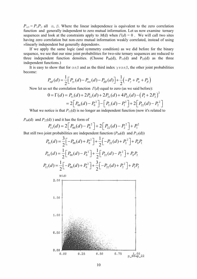
There is an

0. First randomP22 < P2 and frall are non-nega

2.4 Finite-s

So if we wprobabilities {P{cαβ} devided bin the case of particular casenumber of the s

If we leave of the magnitud

as c cαβ αβδ =

where K = ∑α1is why the finit

2.5 Symbolic Dynamic systeorganized critibehind this is thBut let us contisequences, evenumerical valuesuch correlationmethod can't bethe mutual infosites are generaThe Fourier trcharacterizing asuch as white their correlatiostandard way measurements a

Fig.5 Mutual information function versus P00+P22 in ternary sequences when Γ(d) = 0.

easy experiment to show what are possible mutual information values if Γ(d) = ly choose P0 and 0 < P2 < 1 - P0, then randomly choose 0 < P00 < P0 and 0 < om that calculate the rest of the joint probabilities from equation above. And if tive it is possible to calculate the mutual information.

ize effect: overestimation of M(d)

ant to calculate mutual information, we have to have the value of the joint αβ} or in other words the numbers of occurrence for the joint configuration y the total number of counting N, where N is the length of the sequence. But a finite number countings some problems arise. It is shown that in that

we get overestimation that is approximately K(K-2)/2N, where K is the tates for each variable. out all the derivations we get that for the typical fluctuation of the countings is e of the square root of a variable value ( c cαβ αβδ ∼ , are defined

cα− β and c c cα αδ = − α ) . Then

c cα αδ ∼

( 2( ) ( )2

K KM d M dN

)−− ≈

is the total number of states for the variable. K is always grater than 2 and this e-size effect is always overstimation of the mutual information.

noise

ms with expended spatial degress of freedom naturally evolve into self-cal structures of states which are barely stable. There are suggestions that e occurrence of 1/f noise.

nue slowly. As we already said correlation function does not apply to symbolic n if sometimes the correlation of a particular symbol is calculated (the is one if the symbol is present and zero if not). So we have K symbols, for K functions.This is equivalent to Γα(d) = Pαα(d)- Pα

2, where α =1,2,…,K. This used to calculate correlation between different symbols (Pαβ (d)). We see that rmation function (MIF) for such calculation is equal zero if and only if two lly independent or Pαβ = PαPβ for all α,β. ansformation (power spectra) and correlation function are important for nd classifying numeric random sequences or noise. There are different noises,

noise, brownian noise and 1/f noise (they can be distinguished by the form of n function and power spectra). But we have to be aware that there is no to measure correlation in symbolic sequences and that none of this re important for application to DNA molecules and other biopolymers.

11

Wentian Li [3] proposed the name symbolic noise for those symbolic sequences with large value of single-site entropy but many possible forms of MIF. It was further suggested that if the MIF for a symbolic sequences decays to zero even at the nearest neighbor. This kind of sequences can be considered as the symbolic counterpart for white noise. In the case that the MIF decays very slowly the sequences might be something similar to the 1/f α noise, so we can call it symbolic 1/f noise. For the better understanding it's a good idea to look up at some examples in the real world. The simplest examples are letter sequences of natural language text, nucleotide sequences of DNA or RNA molecules and other. And the logical question that follows is what kind of noise are the sequences we are talking about. From this calculation it is visible that the MIF in figure 4 somehow decays in a way in the middle of power low and exponential function (short distances). But it's still possible to approximate the function form by a power law form: M(d) ~ 1/d3. . Till now there was no good name for this kind of (symbolic) noise. The only thing we can be sure of is that it’s not a symbolic 1/f noise, because the correlation measure decays too fast.

Fig.6 Site-to-site M(d) for letter sequences (28 symbols) from (1) Shakepeare's play Hamlet; (2) Associated Press news articles; (3) the five books of Moses from the Bible in German; (4) 11 plays by Shakepeare. The dashed line is an inverse power law function 1/d3. The dotted lines are estimated residual values of M(d) according to K(K - 2)/2N

12

3. Mutual information function and classical poetry 3.1 Introduction to classical poetry For easier understanding of what we will be analizing it's a good idea to make a short overview of the ancient poetry. Of course we will also explain the methodology used to map the verses into a symbolic sequences.

Homer's Iliada and Odysey are two of the chosen works for representing classical greek poetry. Homer is said to be the first to have used the HEXAMETER (a verse of six meters or foots in the above listed works). If we look at these works linguisticaly we notice that there are a lot of formulae (strings of words that repeat themselves in both poems) and epithets (exp. »owl-eyed Athena«). This forms are used to help with the poems rhythm. It is important to say that the hexameter wasn't only used for epic poetry, but also for geners like didactic poetry. An example of such poet was Hesoid who used it in Theogony in an attempt to explain the origins of the universe and the »family tree« of the greek gods. The last example from greek literature that was used is Theocritus's Idylls with which he tried to draw a picture of the simple countryside lifestyle. This and other authors from Syracuse were part of Virgil's inspiration. Something interesting to point out is that both Homer and Hesiod have written in an artificial language that was reserved for poetry and Theocritus used a local dialect. It is also true that the older poetry had a tendency to take distance from the everyday speech because of the search for the rhythm.

As in greek poetry, we will now analize three latin poets: Lucretius, Vergil and Ovid. Lucretius in On the nature of things explains the order in the universe and human's relation to it (his use of the verse is similar to that of Hesiod), Vergil's epic poem Aeneida, which is somehow similar to Odyssey, but lacks formulae and epithets, and didactic Georgics, an agricultural advices book, and in the end Ovid's Metamorphoses that is a collage of myths about gods, semigods and heroes.

Hexameter is, as we said before, a verse of six meters whose basic feature is the diactyl (one long sylable followed by two short ones). Graphically it's represented by:

__ uu | __ uu | __ uu | __ uu | __ uu | __ u,

where __ indicates the long sylable and U the short ones. Another basic feature of the hexameter is a spondee (represented by __ __ ). Note that the different foots are separated by vertical bars. The first foot can be either of the two. So it can be

__ uu | __ uu | __ uu | __ uu | __ uu | __ u or

__ __ | __ __ | __ __| __ __ | __ uu | __ u.

Every foot is formed by a biceps. This last is formed by the first half always long and second half being either short or long.

Another possible hexameter feature is the caesura (pausa). It's usual for the pause to be at the end of word and sometimes even coincides with the foot end. Let us now analyze a verse from the first book in the Aeneida:

Arma virumque cano, Troiae qui primus ab oris and is thus:

__ uu | __ uu | __ ⇑ u| __ uu | __ uu | __ u,

13

where the ⇑ indicates the caesura and in the verse above coincides with the comma. Now we can write the above verse with arsis and thesis (Ta, ta), which are the so called up and down beats.

ARma virUMque caNO, TroiAE qui PRImus ab Oris or

TA-ta-ta TA-ta-ta TA ⇑ ta TA-ta-ta TA-ta-ta TA-ta. It shows that it is convient to map the hexameter into a symbolic time series using a trinary system ( long 0, short 1, pausa 2). For this paper R. Mansilla and E. Bush [1] mapped the first 100 verses of the all listed works. 3.2 Mif and the alphabet for classical poetry

Now that we have became familiar with some basic concepts of both MIF and mapping poetry, we can write (for this work) the alphabet A = {0, 1, 2}, where α, β ∈ A. If we recall the MIF form:

( )

( ) ( ) lnK K P d

M d P dP Pαβ

αβα β α β

≡ ∑∑ .

It's obvious that our sequences are not infinite, but large enough to allow stable statistical estimations of Pαβ (d) , Pα and Pβ.

Such function as the one above have often a periodic behavior. A widely used methode to study those kinds of behavior Fourier spectra (for time series analysis), which is represented in the frequency domain. This representation can easily reveal patterns that can indicate periodical behavior. 3.3 Result and discussion

After introducing the MIF and deciding the way to map the verses, let us now analyse the results Marsilla and Bush got from their analysis.

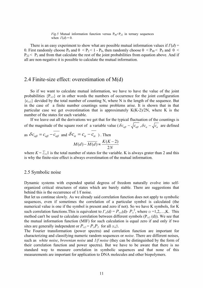
We'll start by analysing the behaviour of MIF related to each verse. In fig. 3.1.a and 3.1.b the change that happened from greek to latin poetry is noticable. The peak at d = 2 is much more pronounced in the Vergil's work. This peak is related to the long syllable common to the dactyl and spondee and the substitution between them. The next peak in Iliad (d=9) almost disappears in Latin poetry, because the verse there is more relaxed. The last big change is that the peak d = 17 in Iliade moves to d = 16 in the Aeneida. This shift is related to the use and the position of the pause. If we take a closer look to the structure of the verse, they used

partial information function (PIF, ( )

( ) ( ) lnP P dM d P d

P Pαβ

αβ αβα β

≡ ).

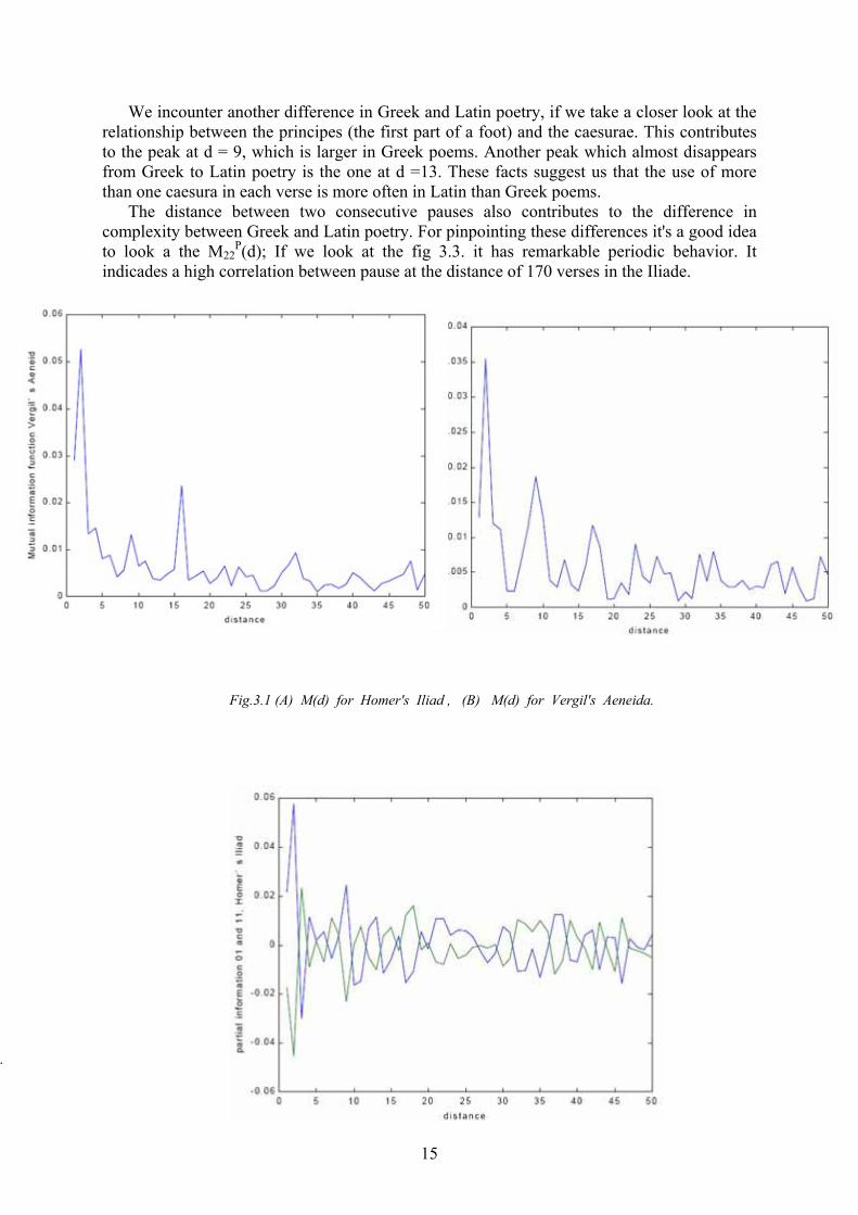
A remarkable property of function M01P(d) and M11

P(d) is that their graphs are mirror images of each other with respect to the horizontal axis. The important consequence of the above property ( M01

P(d) + M11P(d) = 0) is that they don't contribute to MIF. This means that

the peak noticed at the distance d = 2, 9 in the MIF of every poem is contribution to the remainder PIF.

14

We incounter another difference in Greek and Latin poetry, if we take a closer look at the relationship between the principes (the first part of a foot) and the caesurae. This contributes to the peak at d = 9, which is larger in Greek poems. Another peak which almost disappears from Greek to Latin poetry is the one at d =13. These facts suggest us that the use of more than one caesura in each verse is more often in Latin than Greek poems.

The distance between two consecutive pauses also contributes to the difference in complexity between Greek and Latin poetry. For pinpointing these differences it's a good idea to look a the M22

P(d); If we look at the fig 3.3. it has remarkable periodic behavior. It indicades a high correlation between pause at the distance of 170 verses in the Iliade.

.

Fig.3.1 (A) M(d) for Homer's Iliad , (B) M(d) for Vergil's Aeneida.

15

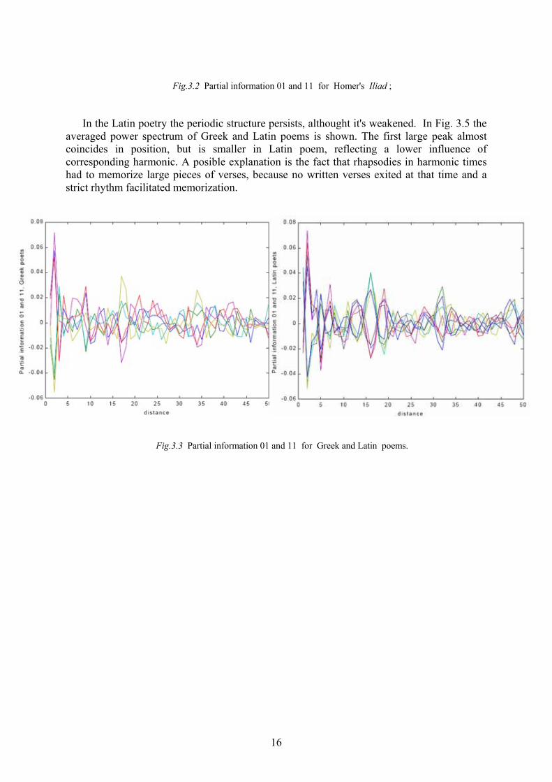
In the Latin poetryaveraged power spectrcoincides in positioncorresponding harmonhad to memorize largestrict rhythm facilitated

Fig.3.2 Partial information 01 and 11 for Homer's Iliad ;

the periodic structure persists, althought it's weakened. In Fig. 3.5 the um of Greek and Latin poems is shown. The first large peak almost , but is smaller in Latin poem, reflecting a lower influence of ic. A posible explanation is the fact that rhapsodies in harmonic times pieces of verses, because no written verses exited at that time and a memorization.

Fig.3.3 Partial information 01 and 11 for Greek and Latin poems.

16

Fig.3.4 (A) Partial information 22 for Homer's Iliad , (B ) Partial information 22 for Homer's Odissey and (C) Partial information 22 for Lucretiu's Nature of Things.

17

Fig

4. Conclus The use that wthat the strucAnd we can There are difintroduction oIt is importanstudy of natuother researcsymbolic sequ 5. Referen [1] R.MansillAssociation fwas held at N[2] W. Li, MuSFI-89- 008, [31] W. Li, MPhysics, Vol.[42] M. Gardfluctation, Sc [5] Douglas DAmerica, (19

.3.5 Avarage power spectrum for Greek and Latin poems; The Latin is green.

ion

as illustrated in this paper is only one possible use of the MIF. The results show ture changes or better increases in complexity from the Greek to Latin poetry. notice some major differences even in the evolution of the Greek poetry itself. ferent explanation of why is so. One of the explanations for this increase is the f writing in poetry instead of memorizing large parts of poems. t to point out the MIF is mostly used for DNA researching. Nevertheless the

ral languages opens the area of the »speech« of artificial intelligence and many hes that were almost not possible before the start of use of this method for ences analysis.

ces

a, E. Bush, Increase of Complexity from Greek to Latin Poetry, submitted to or Integrative Studies Journal, Interdisciplinary Studies and Complexity which ational Autonomuos University of Mexico, (2001) tual inforation function of natural language texts, Santa Fe Institute preprints,

(1989) utual inforation function versus Correlation functions, Journal of Statistical

6, (1990) ner, Mathematical Ggames: White and brown music, fractal curves and 1/f i. Am 238(4): 16-32 (1978)

. Mooney, A course in mathematical modeling, Mathematical Association of 99)

18