COMPLEXITY-DISTOR TRADEOFFS IN AND VIDEO - USCsipi.usc.edu/~ortega/PhDTheses/KrisdaLengwehasatit.pdf · COMPLEXITY-DISTOR TION TRADEOFFS IN IMA GE AND VIDEO COMPRESSION b y ... CA)

COMPLEXITY-DISTORTION TRADEOFFS IN IMAGE AND VIDEO

COMPRESSION

by

Krisda Lengwehasatit

A Dissertation Presented to the

FACULTY OF THE GRADUATE SCHOOL

UNIVERSITY OF SOUTHERN CALIFORNIA

in Partial Ful�llment of the

Requirements for the Degree

DOCTOR OF PHILOSOPHY

(ELECTRICAL ENGINEERING)

May 2000

Copyright 2000 Krisda Lengwehasatit

Contents

List of Figures v

List of Tables xiii

Abstract xiv

1 Introduction 1

1.1 Overview of compression . . . . . . . . . . . . . . . . . . . . . . . 1

1.2 Rate-distortion and complexity . . . . . . . . . . . . . . . . . . . 3

1.3 Variable Complexity Algorithm (VCA) . . . . . . . . . . . . . . . 5

1.4 Discrete Cosine Transform Algorithms . . . . . . . . . . . . . . . 7

1.4.1 De�nition of DCT . . . . . . . . . . . . . . . . . . . . . . 7

1.4.2 Exact vs. Approximate DCT . . . . . . . . . . . . . . . . 9

1.4.3 VCA DCT . . . . . . . . . . . . . . . . . . . . . . . . . . . 13

1.4.4 Computationally Scalable DCT . . . . . . . . . . . . . . . 16

1.4.5 Thesis Contributions . . . . . . . . . . . . . . . . . . . . . 16

1.5 Motion Estimation . . . . . . . . . . . . . . . . . . . . . . . . . . 17

1.5.1 Example: Conventional Exhaustive Search . . . . . . . . . 18

1.5.2 Fast Search vs. Fast Matching . . . . . . . . . . . . . . . . 20

1.5.3 Fixed vs. Variable Complexity . . . . . . . . . . . . . . . . 22

1.5.4 Computationally Scalable Algorithms . . . . . . . . . . . . 23

1.5.5 Thesis Contributions . . . . . . . . . . . . . . . . . . . . . 24

1.6 Laplacian Model . . . . . . . . . . . . . . . . . . . . . . . . . . . 25

ii

2 Inverse Discrete Cosine Transform 29

2.1 Formalization of IDCT VCA . . . . . . . . . . . . . . . . . . . . . 30

2.1.1 Input Classi�cation . . . . . . . . . . . . . . . . . . . . . . 31

2.2 Proposed VCA for IDCT . . . . . . . . . . . . . . . . . . . . . . . 34

2.2.1 Sequential Classi�cation . . . . . . . . . . . . . . . . . . . 34

2.2.2 Greedy Optimization . . . . . . . . . . . . . . . . . . . . . 35

2.2.3 Tree-structured classi�cation (TSC) . . . . . . . . . . . . . 37

2.2.4 Optimal Tree-structured Classi�cation (OTSC) . . . . . . 39

2.2.5 Computation of 2-D IDCT . . . . . . . . . . . . . . . . . . 43

2.2.6 2-D Dyadic Classi�cation . . . . . . . . . . . . . . . . . . . 44

2.3 Results . . . . . . . . . . . . . . . . . . . . . . . . . . . . . . . . . 45

2.3.1 Results Based on Image Model . . . . . . . . . . . . . . . 47

2.3.2 Real Image Data Results . . . . . . . . . . . . . . . . . . . 50

2.4 Distortion/decoding time tradeo�s . . . . . . . . . . . . . . . . . 54

2.5 Rate-Complexity-Distortion Quadtree Optimization . . . . . . . . 58

2.6 Summary and Conclusions . . . . . . . . . . . . . . . . . . . . . . 63

3 Forward Discrete Cosine Transform 65

3.1 Exact VCA DCT . . . . . . . . . . . . . . . . . . . . . . . . . . . 66

3.1.1 Input Classi�cation: Pre-transform Deadzone Test . . . . . 66

3.1.2 Optimal Classi�cation . . . . . . . . . . . . . . . . . . . . 71

3.2 Approximate DCT . . . . . . . . . . . . . . . . . . . . . . . . . . 72

3.2.1 SSAVT Review . . . . . . . . . . . . . . . . . . . . . . . . 73

3.2.2 Error Analysis of SSAVT . . . . . . . . . . . . . . . . . . . 75

3.2.3 APPROX-Q DCT . . . . . . . . . . . . . . . . . . . . . . . 80

3.2.4 APPROX-Q Error Analysis . . . . . . . . . . . . . . . . . 84

3.3 Results and Hybrid Algorithms . . . . . . . . . . . . . . . . . . . 86

3.3.1 Approx-SSAVT (ASSAVT) . . . . . . . . . . . . . . . . . . 87

3.3.2 Approx-VCA DCT . . . . . . . . . . . . . . . . . . . . . . 89

3.3.3 ASSAVT-VCA DCT . . . . . . . . . . . . . . . . . . . . . 89


4 Motion Estimation: Probabilistic Fast Matching 91

4.1 Partial Distance Fast Matching . . . . . . . . . . . . . . . . . . . 92

4.2 Hypothesis Testing Framework . . . . . . . . . . . . . . . . . . . . 96

4.3 Parameter Estimation . . . . . . . . . . . . . . . . . . . . . . . . 100

4.3.1 Model Estimation for ROW . . . . . . . . . . . . . . . . . 101

4.3.2 Model Estimation for UNI . . . . . . . . . . . . . . . . . . 102

4.4 Experimental Results . . . . . . . . . . . . . . . . . . . . . . . . . 106

4.4.1 VCA-FM versus VCA-FS . . . . . . . . . . . . . . . . . . 107

4.4.2 UNI versus ROW . . . . . . . . . . . . . . . . . . . . . . . 109

4.4.3 Scalability . . . . . . . . . . . . . . . . . . . . . . . . . . . 110

4.4.4 Temporal Variation . . . . . . . . . . . . . . . . . . . . . . 112

4.4.5 Overall Performance . . . . . . . . . . . . . . . . . . . . . 113

4.5 HTFM for VQ . . . . . . . . . . . . . . . . . . . . . . . . . . . . . 113


5 Motion Estimation: PDS-based Candidate Elimination 119

5.1 PDS-based Candidate Elimination . . . . . . . . . . . . . . . . . . 120

5.1.1 Ideal Candidate Elimination . . . . . . . . . . . . . . . . . 122

5.1.2 Reduced Steps Candidate Elimination . . . . . . . . . . . 123

5.2 Suboptimal CE-PDS . . . . . . . . . . . . . . . . . . . . . . . . . 126

5.2.1 Computationally Nonscalable Fast Search . . . . . . . . . 126

5.2.2 Computationally Scalable Fast Search . . . . . . . . . . . . 128

5.3 Multiresolution Algorithm . . . . . . . . . . . . . . . . . . . . . . 130


Bibliography 136

List of Figures

1.1 (a) Video encoding and (b) decoding system. . . . . . . . . . . . . 2

1.2 Variable complexity algorithm scheme. . . . . . . . . . . . . . . . 5

1.3 A fast (a) DCT (b) IDCT algorithm introduced by Vetterli-Ligtenberg

where 'Rot' represents the rotation operation which takes inputs

[x; y] and produces outputs [X; Y ] such that X = x cosQ+ y sinQ

and Y = �x sinQ+ y cosQ, C4 = 1=p2. . . . . . . . . . . . . . . 10

1.4 Frequency of nonzero occurrence of 8x8 quantized DCT coeÆcients

of \lenna" image at (a) 30.33 dB and (b) 36.43 dB. . . . . . . . . 14

1.5 Frequency of nonzero occurrence of 8x8 quantized DCT coeÆcients

of 10 frames for \Foreman" at QP=10 (a) I-frame (b) P-frame. . . 14

1.6 Motion estimation of i-th block of frame t predicted from the best

block in the search region � in frame t-1. . . . . . . . . . . . . . . 18

1.7 Summary of ST1 algorithm where (a) and (b) depict spatial and

spatio-temporal candidate selection, respectively. Highlighted blocks

correspond to the same spatial location in di�erent frames, (c) illus-

trates the local re�nement starting from the initial motion vector

found to be the best among the candidates. . . . . . . . . . . . . 22

1.8 Rate-Distortion using standard-de�ned DCT ('dashed') and R-D

for SSAVT ('solid') for �2 = 100 with varying QP at 3 block sizes,

i.e., 4x4, 8x8 and 16x16. The rate and distortion is normalized to

per pixel basis. . . . . . . . . . . . . . . . . . . . . . . . . . . . . 28

2.1 TSC pseudo code for testing upper 4 branches of Fig. 1.3 (b) in

stage 2. . . . . . . . . . . . . . . . . . . . . . . . . . . . . . . . . 38

v

2.2 TSC diagram showing zero information of classes after all-zero test

and 4-zero tests. . . . . . . . . . . . . . . . . . . . . . . . . . . . . 39

2.3 TSC diagram showing zero information of classes after 2-zero test

and 1-zero tests. The most right-handed class after 2-zero test

is further classi�ed into 9 classes which are tensor products of

descendent classes shown, i.e., A B = f(Ai \ Bj)g8 i;j where

A = fAig; B = fBig. Therefore, the number of leaves is 3+3+(3x3)= 15. . . . . . . . . . . . . . . . . . . . . . . . . . . . . . . . . . . 40

2.4 Diagram showing possible choices for classi�cation at level 2 where

A, B represent testing with M [1010] and M [0101], respectively. . 41

2.5 Another diagram when the result from level 1 is di�erent. . . . . . 41

2.6 Content of bitmap after �rst (row-wise) 1-D IDCT where 'x' rep-

resents nonzero coeÆcient. . . . . . . . . . . . . . . . . . . . . . . 43

2.7 Dyadic classi�cation scheme. A DCT input of size NxN is classi�ed

into all-zero, DC-only (K1), low-2x2 (K2),..., low-N2xN

2(KN=2), and

full-NxN (KN ) classes. . . . . . . . . . . . . . . . . . . . . . . . 44

2.8 Number of additions (a) and the number of multiplications (b)

needed for �2 = 100 and 700, using OTSC ('solid'), Greedy ('dashed'),

Ideal fast IDCT ('dashed-dotted'), and Ideal matrix multiplication

('light-solid'). The OTSC and Greedy are optimized for each QP. 47

2.9 Total complexity (a) and the number of tests (b) needed for �2 =

100 and 700 using OTSC ('solid') and greedy ('dashed') algorithms. 48

2.10 (a) Complexity-distortion and (b) Rate-complexity curves for dif-

ferent algorithms, i.e., greedy ('dotted') and 2-D dyadic ('dashed'),

for DCT size 16x16 ('x'), 8x8 ('o') and 4x4 ('*') at �2 = 100. The

complexity unit is weighted operations per 64 pixels. . . . . . . . 49

2.11 Normalized estimated complexity for \lenna" using CW with all-

zero test algorithm ('+'), CW with all-zero test for the �rst 1-D

IDCT and ac-zero test for the second 1-D IDCT ('x'), FW algo-

rithm ('*'), and OTSC algorithm ('o'). . . . . . . . . . . . . . . . 50

2.12 Normalized actual time complexity (only IDCT algorithm part) for

\lenna" using CW with all-zero test algorithm ('+'), CW with all-

zero test for the �rst 1-D IDCT and ac-zero test for the second 1-D

IDCT ('x'), FW algorithm ('*'), and OTSC algorithm ('o'). . . . . 51

2.13 Normalized actual time complexity (total decoding time) for \lenna"

using CW with all-zero test algorithm ('+'), CW with all-zero test

for the �rst 1-D IDCT and ac-zero test for the second 1-D IDCT

('x'), FW algorithm ('*'), OTSC algorithm ('o'). OTSC for lenna

at MSE 14.79 ('{'), and OTSC for lenna at MSE 60.21 ('-.'). . . . 52

2.14 Normalized actual time complexity (total decoding time) for ba-

boon image using CW with all-zero test algorithm ('+'), CW with

all-zero test for the �rst 1-D IDCT and ac-zero test for the second

1-D IDCT ('x') , FW algorithm ('*'), OTSC algorithm ('o'), and

OTSC for lenna with MSE 14.79 ('{') . . . . . . . . . . . . . . . . 53

2.15 The complexity (CPU clock cycle) of the IDCT + Inv. Quant.

normalized by the original algorithm in TMN at various PSNRs

(di�erent target bit rates) using OTSC ('4') and combined dyadic-OTSC ('*'). . . . . . . . . . . . . . . . . . . . . . . . . . . . . . 54

2.16 Distortion versus (a) estimated IDCT complexity (b) experimen-

tal decoding time of \lenna" using �xed quantizer encoder and

OTSC decoder ('o'), Lagrange multiplier results ('x'), encoder fol-

lows Lagrange multiplier results but decoder uses a single OTSC

for MSE=60.66 ('*') and MSE=14.80 ('+'), respectively. . . . . . 56

2.17 (a) Complexity-Distortion curve obtained from C-D ('x') and R-D

('*') based optimization. (b) Rate-Distortion curve achieved when

C-D ('x') and R-D ('*') based optimization. The complexity is

normalized by the complexity of the baseline Vetterli-Ligtenberg

algorithm. . . . . . . . . . . . . . . . . . . . . . . . . . . . . . . . 57

2.18 Quadtree structures of four 16x16 regions and the corresponding

representative bits. . . . . . . . . . . . . . . . . . . . . . . . . . . 59

2.19 Constant-complexity rate-distortion curves. When complexity con-

straint is loosen, the rate-distortion performance can be better.

'dashed' curves show unconstrained complexity result. . . . . . . . 61

2.20 Constant-rate complexity-distortion curves at 200 Kbps and 300

Kbps. As rate is more constrained, C-D performance gets worse. . 62

2.21 Constant-distortion rate-complexity curves at MSE = 30 and 50.

As distortion requirement is more rigid, the R-C performance be-

comes worse. . . . . . . . . . . . . . . . . . . . . . . . . . . . . . . 63

3.1 Geometric representation of dead-zone after rotation. . . . . . . . 68

3.2 Proposed VCA algorithm. . . . . . . . . . . . . . . . . . . . . . . 69

3.3 Comparisons of original and pruned algorithms for di�erent distor-

tions (a) number of additions, (b) number of multiplications. The

DCT lower bound corresponds to computing only the subset of co-

eÆcients that will be non-zero after quantization. The VCA lower

bound corresponds to pruning subject to the classi�cation mecha-

nisms of Section 3.1.2, i.e., we can only prune subsets of coeÆcients

which are tested jointly. . . . . . . . . . . . . . . . . . . . . . . . 70

3.4 Complexity(clock cycle)-distortion comparison with \lenna" JPEG

encoding. . . . . . . . . . . . . . . . . . . . . . . . . . . . . . . . 72

3.5 Additional distortion (normalized by the original distortion) when

using SSAVT at various levels of the pixel variance �2. . . . . . . 76

3.6 Rate-complexity-distortion functions of SSAVT. The R-C-D results

of SSAVT and ideal dyadic test are very close and hence cannot be

visually distinguished in the �gure. . . . . . . . . . . . . . . . . . 78

3.7 Total complexity and the number of tests needed for SSAVT al-

gorithms and 2-D dyadic at �2 = 100 and 700. 2-D dyadic is

considered as an ideal case for the SSAVT where reduced classes

are 100% detected. . . . . . . . . . . . . . . . . . . . . . . . . . . 79

3.8 (a) Complexity-distortion and (b) Rate-complexity curves for dif-

ferent algorithms, i.e., SSAVT ('solid') and 2-D dyadic ('dashed'),

for DCT size 16x16 ('x'), 8x8 ('o') and 4x4 ('*') at �2 = 100. 2-D

dyadic is considered as an ideal case for the SSAVT where reduced

classes are 100% detected. . . . . . . . . . . . . . . . . . . . . . . 80

3.9 The approximate DCT algorithm. . . . . . . . . . . . . . . . . . . 81

3.10 Rate-Distortion curve of 512x512 lenna image JPEG coding us-

ing various DCT algorithms. Note that at high bit rate coarser

approximate algorithm performances deviate from the exact DCT

performance dramatically. The quantization dependent approxi-

mation can maintain the degradation level over wider range of bit

rate. . . . . . . . . . . . . . . . . . . . . . . . . . . . . . . . . . . 83

3.11 Additional distortion (normalized by original distortion) using ap-

proximate DCT algorithms #1 ('�'), #2 ('5'), #3 ('o'), #4 (''),and #5 ('�') at various pixel variance �2. . . . . . . . . . . . . . 85

3.12 The complexity (CPU clock cycle) of the DCT + Quant. normal-

ized by the original algorithm in TMN at various PSNRs (di�erent

target bit rates) of original DCT ('+'), SSAVT ('o'), Approx-Q

('4'), ASSAVT ('2'), Approx-VCA ('5'), and ASSAVT-VCA ('*'). 87

3.13 Additional distortion (normalized by original distortion) using the

ASSAVT with 2x10�4 target deviation from the original distortion

('- -'), SSAVT ('{'), at QP = 10 ('o') and 22 ('*'), respectively. . . 88

4.1 Subset partitionings for 128 pixels subsampled using a quincunx

grid into 16 subsets for partial SAD computation. Only highlighted

pixels are used to compute SAD. Two types of subsets are used

(a) uniform subsampling (UNI) and (b) row-by-row subsampling

(ROW). Partial distance tests at the i-th stage are performed after

the metric has been computed on the pixels labeled with i (corre-

sponding to yi). . . . . . . . . . . . . . . . . . . . . . . . . . . . . 94

4.2 Complexity-Distortion of reduced set SAD computation with ROW

DTFM ('dotted') and without DTFM ('solid') using (a) ES and (b)

ST1 search, averaged over 5 test sequences. Points in each curve

from right to left correspond to j�j = 256, 128, 64 and 32, respec-

tively. Note that there is a minimal di�erence between computing

the SAD based on 256 and 128 pixels. For this reason in all the

remaining experiments in this work we use at most 128 pixels for

the SAD computation. . . . . . . . . . . . . . . . . . . . . . . . . 95

4.3 (a) Scatter plot between MAD (y-axis) and PMADi (x-axis) and

(b) corresponding histograms of MAD�PMADi. These are plot-

ted for 16 stages of UNI subsampling, with number of pixels ranging

from 8 (top left) to 128 (bottom right). We use UNI subsampling

and ES on the \mobile &calendar" sequence. Similar results can

be obtained with other sequences, search methods and subsampling

grids. . . . . . . . . . . . . . . . . . . . . . . . . . . . . . . . . . . 97

4.4 Empirical pdf ofMAD�PMADi (estimation error) obtained from

histogram of training data (solid line) and the corresponding para-

metric model (dashed line). HTFM terminates the matching metric

computation at stage i if PMADi �MADbsf > Thi. . . . . . . . 99

4.5 (a)�2i and (b) ~�2

i of ROW computed from the de�nition (mean

square) ('solid') and computed from the �rst order moment ('dashed').

The left-most points in (a) are Ef(PMAD1 � PMAD2)2g and

2EfjPMAD1 � PMAD2jg2. . . . . . . . . . . . . . . . . . . . . . 103

4.6 (a) �2i ('solid') and 2�2

i ('dashed') of MAD estimate error at 15

stages using ES and UNI, respectively. The left-most points shows

Ef(PMAD1�PMAD2)2g and 2EfjPMAD1�PMAD2jg2 for each

sequence. (b) Ratio of �2i =�

21 for each sequence. Note that this ratio

is nearly the same for all sequences considered. . . . . . . . . . . 105

4.7 Example of tracking of statistics �i under UNI subsampling. Note

that the approximated values track well the actual ones, even though

the parameters do change over time. We use several di�erent se-

quences to provide the comparison. This serves as motivation for

using online training, rather than relying on precomputed statistics. 107

4.8 Complexity-Distortion curve for �rst 100 frames of \mobile" se-

quence (a) with MSE of the reconstructed sequence and (b) with

residue energy as distortion measures and search without test ('o'),

partial distance (SAD� test) ('*') and combined hypothesis-SAD�

test ('x') each curve at �xed Pf labeled on each curve and varying

� from 0.01-4. . . . . . . . . . . . . . . . . . . . . . . . . . . . . . 108

4.9 Complexity-distortion of HTFM with ES and variance estimation

on-the- y, ROW ('solid') and UNI ('dashed'), (a) PSNR degrada-

tion vs. clock cycle and (b) residue energy per pixel vs. number of

pixel-di�erence operations. Both clock cycle and number of pixel-

di�erence operations are normalized by the result of ES with ROW

DTFM. It can be seen that UNI HTFM performs better than ROW

HTFM. The transform coding mitigates the e�ect of the increase of

residue energy in the reconstructed frames. The testing overhead

reduces the complexity reduction by about 5%. The complexity

reduction is upto 65% at 0.05 dB degradation. . . . . . . . . . . 110

4.10 Complexity-distortion of UNI HTFM with variance estimation on-

the- y of (a) 2-D Log search and (b) ST1 search. The axes are clock

cycle and PSNR degradation normalized/compared to the 2-D Log

search (a) or ST1 search (b) with ROW DTFM. The complexity

reduction is upto 45% and 25% at 0.05 dB degradation for 2-D Log

and ST1 search, respectively. . . . . . . . . . . . . . . . . . . . . . 111

4.11 Frame-by-frame speedup factor for ES using ROW and DTFM

('�'), and ROW HTFM ('o') with Pf = 0.1 and 0.01 dB degra-

dation. . . . . . . . . . . . . . . . . . . . . . . . . . . . . . . . . 112

4.12 Frame-by-frame speedup factor for 2-D Log search using ROW and

no FM ('*'), DTFM ('�'), and ROW HTFM ('o') with Pf = 0.2

and 0.04 dB degradation. . . . . . . . . . . . . . . . . . . . . . . 113

4.13 Frame-by-frame speedup factor for ST1 algorithm using ROW and

no FM ('*'), DTFM ('�'), and ROW HTFM ('o') with Pf = 0.3

and 0.12 dB degradation. . . . . . . . . . . . . . . . . . . . . . . . 114

4.14 Complexity-distortion of HTFM VQ with vector size (a) 8 for i.i.d.

source and (b) 16 (4x4) for high-high band of \lenna" image. . . . 117

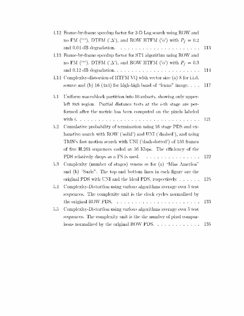
5.1 Uniform macroblock partition into 16 subsets, showing only upper-

left 8x8 region. Partial distance tests at the i-th stage are per-

formed after the metric has been computed on the pixels labeled

with i. . . . . . . . . . . . . . . . . . . . . . . . . . . . . . . . . . 121

5.2 Cumulative probability of termination using 16 stage PDS and ex-

haustive search with ROW ('solid') and UNI ('dashed'), and using

TMN's fast motion search with UNI ('dash-dotted') of 150 frames

of �ve H.263 sequences coded at 56 Kbps. The eÆciency of the

PDS relatively drops as a FS is used. . . . . . . . . . . . . . . . 122

5.3 Complexity (number of stages) versus m for (a) \Miss America"

and (b) \Suzie". The top and bottom lines in each �gure are the

original PDS with UNI and the ideal PDS, respectively. . . . . . . 125

5.4 Complexity-Distortion using various algorithms average over 5 test

sequences. The complexity unit is the clock cycles normalized by

the original ROW PDS. . . . . . . . . . . . . . . . . . . . . . . . 133

5.5 Complexity-Distortion using various algorithms average over 5 test

sequences. The complexity unit is the the number of pixel compar-

isons normalized by the original ROW PDS. . . . . . . . . . . . . 135

List of Tables

1.1 Pro�le of component in MPEG2 encoder for the sequence \mo-

bile& calendar". ES: exhaustive search, ST1: a spatio-temporal

fast search [4], PDS: partial distance search. . . . . . . . . . . . . 3

1.2 Number of operations required to compute a 1-D size N DCT using

various fast algorithms (the number in the brackets is obtained

when N=8). . . . . . . . . . . . . . . . . . . . . . . . . . . . . . . 11

1.3 Notation Table . . . . . . . . . . . . . . . . . . . . . . . . . . . . 19

2.1 Weight for di�erent logical operations. . . . . . . . . . . . . . . . 46

3.1 Number of operations required for proposed approximate algorithms

where Alg. No. i corresponds to using the transform matrix Poi. . 82

4.1 Total time for encoding 150 frames and PSNR. . . . . . . . . . . . 115

4.2 cont. Total time for encoding 150 frames and PSNR. . . . . . . . 116

5.1 Number of PSAD metric computation stages for di�erent PDS vari-

ation for 150 frames of H.263 sequences coded at 56 Kbps. . . . . 124

5.2 Results of 2-FCE complexity reduction with respect to the original

PDS. . . . . . . . . . . . . . . . . . . . . . . . . . . . . . . . . . . 127

5.3 Results of 8-FCE (2 stage PSAD per 1 step testing). . . . . . . . 128

5.4 Result of using UBC's Fastsearch option. . . . . . . . . . . . . . . 128

5.5 Result of 2-Step with Threshold when m = 1 and t = 1. . . . . . . 130

5.6 Results of MR1-FCE and MR2-FCE complexity reduction at t =

0:8 with respect to the original multiresolution algorithm. . . . . . 133

xiii

Abstract

With the emergence of the Internet, a broader range of information transmission

such as text, image, video, audio, etc. is now ubiquitous. However, the growth

of data transferring is not always matched by the growth in available channel

bandwidth. This has raised the importance of compression especially for images

and video. As a consequence, compression standards for image and video have

been developed since the early 90's and have become widely used. Those stan-

dards include JPEG [1] for still image coding, MPEG1-2 [2] for video coding and

H.261/263 [3] for video conferencing.

We are motivated by observing that general purpose workstations and PCs

have increased their speed to a level where performing compression/decompression

in software of images and even video, can be done eÆciently at, or near, real-time

speed. Examples of this trend include software-only decoders for the H.263 video

conferencing standard, as well as the wide use of software implementations of

the JPEG standard to exchange images over the Internet. This trend is likely to

continue as faster processors become available and innovative uses of software, for

example usage of JAVA applets, become widespread. Optimizing the performance

of the algorithms for the speci�c case of software operation is becoming more

important.

In this thesis we investigate variable complexity algorithms. The complexities

of these algorithms are input-dependent, i.e., the type of input determines the

complexity required to complete the operation. The key idea is to enable the

algorithm to classify the inputs so that unnecessary operations can be pruned.

The goal of the design of the variable complexity algorithm is to minimize the

average complexity over all possible input types, including the cost of classifying

the inputs. We study two of the fundamental operations in standard image/video

compression, namely, the discrete cosine transform (DCT) and motion estimation

xiv

(ME).

We �rst explore variable complexity in inverse DCT by testing for zero inputs.

The test structure can also be optimized for minimal total complexity for a given

inputs statistics. In this case, the larger the number of zero coeÆcients, i.e.,

the coarser the quantization stepsize, the greater the complexity reduction. As a

consequence, tradeo�s between complexity and distortion can be achieved.

For direct DCT we propose a variable complexity fast approximation algo-

rithm. The variable complexity part computes only DCT coeÆcients that will

not be quantized to zeros according to the classi�cation results (in addition the

quantizer can bene�t from this information by by-passing its operations for zero

coeÆcients ). The classi�cation structure can also be optimized for a given in-

put statistics. On the other hand, the fast approximation part approximates the

DCT coeÆcients with much less complexity. The complexity can be scaled, i.e.,

it allows more complexity reduction at lower quality coding, and can be made

quantization-dependent to keep the distortion degradation at a certain level.

In video coding, ME is the part of the encoder that requires the most com-

plexity and therefore achieving signi�cant complexity reduction in ME has always

been a goal in video coding research. There have been several algorithms with

variable complexity for ME. However, most of the research concentrate on reduc-

ing the number of tested vector points. We propose two fast algorithms based

on fast distance metric computation or fast matching approaches. Both of our

algorithms allow computational scalability in distance computation with graceful

degradation in the overall image quality. The �rst algorithm exploits hypothesis

testing in fast metric computation whereas the second algorithm uses thresholds

obtained from partial distances in hierarchical candidate elimination.

xv

Chapter 1

Introduction

1.1 Overview of compression

All current image and video compression standards are based on the same concept

of transform based coding, illustrated by Figure 1.1. Basic building blocks of a

transform based image/video encoder include (i) blocking, where data is parti-

tioned into a smaller unit known as block (with size 8x8 pixels) or macroblock

(16x16 pixels), (ii) motion estimation (ME) in predictive mode of video coding

to exploit the temporal redundancy, (iii) Discrete Cosine Transform (DCT) to

decompose the signal into its di�erent frequency components, (iv) quantization to

reduce the amount of information down to a level suitable for the channel (while

introducing distortion) and (v) entropy coding to compress the quantized data

losslessly. The decoding operation performs entropy decoding, inverse quantiza-

tion, inverse DCT (IDCT) and motion compensation, sequentially to obtain the

reconstructed sequence.

Typically, standards de�ne only the syntax of the bit-stream and the decod-

ing operation. They normally leave some room for performance improvement via

better bit allocation at the encoders. Usually the more recent standards which

provide better compression performance, have also more funtionalities and require

more complex operation. With the existing standards, the coding gain comes at

the price of signi�cant complexity at major components of the basic structure such

1

DCT Quantization

InverseQuantization

Frame Buffer MotionCompensation

MotionEstimation

EntropyEncoding

Inverse DCT

+

+MV

-

(a)

InverseQuantization

Frame Buffer MotionCompensation

EntropyDecoding

Inverse DCT +

MV

(b)

Figure 1.1: (a) Video encoding and (b) decoding system.

as DCT, inverse DCT and motion estimation. With the advent of real-time ap-

plications such as video conferencing, complexity issues of the codec have become

more important. In many applications, including decoding on general purpose

computers or on portable devices, signi�cant complexity reduction is needed be-

fore video can be supported, especially if high resolution is required. Table 1.1

shows an example of a typical pro�le of computational complexity, listing the

percentage of time spent in each of the major components in MPEG2 encoding.

We can see that in a video encoding system, motion estimation is the most time

consuming task. With fast motion search, one can achieve speedups of a factor

of 4-5. However, the complexity still remains signi�cant. Besides ME, video en-

coders have to perform DCT/IDCT, which is also a major complexity component.

In Chapter 2-5, we will study the complexity-distortion tradeo� of these two com-

ponents (DCT and ME) based on a variable complexity algorithm framework in

which the complexity is input-dependent. We will propose algorithms such that

2

Table 1.1: Pro�le of component in MPEG2 encoder for the sequence \mobile&

calendar". ES: exhaustive search, ST1: a spatio-temporal fast search [4], PDS:

partial distance search.

component ES ES-PDS ST1 ST1-PDS

Motion estimation 86.6% 69.3% 22.9% 20.2%

Quant. + Inv.Quant 3.7% 8.3% 20.0% 21.7%

DCT + IDCT 1.9% 5.9% 13.0% 12.6%

Others 7.8% 16.5% 44.1% 45.5%

Relative total time 1 0.44 0.2142 0.2106

their structure can be optimized for a given type of input sequences or images, so

that the total complexity is minimal on the average sense.

1.2 Rate-distortion and complexity

In information theory, entropy is de�ned as a measure of the amount of infor-

mation contained in random data. The amount of information can be expressed

in terms of the number of bits needed to represent the data, so that more bits

are needed to represent data containing more information. Entropy represents

the amount of average information of a random source and also serves as a lower

bound for the average code length needed to represent that source. The entropy

of a random sequence �X is de�ned as

H( �X) = �Xx

p(�x) log p(�x) bits

where p(�x) is probability mass function. An entropy encoder maps source symbol

to codeword, E : �x ! c(�x). From information theory one cannot compress data

beyond the entropy (Shannon's source coding theorem). If we want to further

compress the data, distortion must be introduced as a tradeo� and the goal is

to �nd the minimal rate for a given distortion (Shannon's Rate-Distortion theo-

rem [5]), i.e., one wants to �nd a coder with minimal rate for a given distortion

constraint. Similar to the entropy, the rate-distortion function is de�ned as the

3

minimum rate such that the average distortion satis�es a distortion constraint.

Image and video compression algorithms aim at achieving the best possible

Rate-Distortion (R-D) performance. Three main approaches are typically con-

sidered to improve R-D performance, namely, better transformation ([6, 7, 8]),

quantization bit allocation ([9, 10, 11]), and eÆcient entropy coding ([12]). There

are a number of algorithms that provide high eÆciency in each of these areas.

Examples include using the wavelet transform with progressive quantization and

eÆcient entropy coding ([13, 14, 15, 16, 17, 18]), DCT with optimal thresholding

and quantization [19], DCT with progressive coding [20], variable block size DCT

[21], etc. Moreover, in all the above methods, complexity is not taken into account

explicitly.

Shannon's Rate-Distortion theorem provides only an asymptotic result which

is only valid for in�nite memory coders. Typically, encoders with longer memory,

more computational power and larger context statistics can perform better than

encoders using less resources. In complexity-constrained environment, such as in

software implementation of real-time video en/de-coding systems and in battery-

limited pervasive devices, complexity becomes a major concern in addition to

rate-distortion performance. Normally, one would prefer to have a system that

encodes or decodes with higher frame rate with a small degradation in picture

quality rather than to have a slightly better rate-distortion performance with much

more complexity or delay. Thus, in order to achieve the best of rate-distortion-

complexity performance, all three factors must be explicitly considered together.

With the fast increase in the clock speed and performance of general purpose

processors, software-only solutions for image and video encoding/decoder are of

great interest. Software solutions result in not only cheaper systems, since no

specialized hardware needs to be bought, but also provide extra exibility as com-

pared to a customized hardware. In a software implementation, there are many

factors that impact the computational complexity in addition to the number of

arithmetic operations. For example, conditional logic, memory access or caching,

all have an impact in overall speed. However, most of the work that has studied

complexity issues has focused on arithmetic operation (additions and multiplica-

tions), and generally has not considered other factors. The work by Gormish [22]

4

and Goyal [23] are examples of research that addresses complexity-rate-distortion

tradeo�s. In this research the transform block size is used to control the com-

plexity, i.e., when the block size increases, the required complexity also increases

while rate-distortion performance improves. Note, however, that complexity is

determined only by the block size, and therefore, it is constant regardless of the

input. Thus, as in most earlier work in this topic, complexity is analyzed only as

a worst-case. Instead, in this thesis we will concentrate on algorithms designed

to perform well on average.

1.3 Variable Complexity Algorithm (VCA)

In this work, we are interested in reducing the computational complexity of an

algorithm, where complexity could be measured as actual elapsed time, CPU

clock cycle or the number of operations consumed by the process. We develop

algorithms with input-dependent complexity (see Fig. 1.2), such that for some

types of input the complexity is signi�cantly reduced, whereas for some other types

the complexity may be larger than the original complexity (i.e., that achieved with

an input-independent algorithm). For example, the IDCT does not have to be

performed if the input block is all zero. The overhead cost of testing for the all-zero

block is then added to the complexity of not-all-zero block, but, if the percentage

of all-zero block is large enough, the complexity savings can outweigh the testing

overhead. The same can be applied to more sophisticated VCAs in which the

�nal goal is to achieve less complexity on the average. We will show that by using

VCAs, it is possible to achieve a better complexity-distortion performance for a

given rate than reported in [22].

Classifier

Algorithm 1

Algorithm 2

Algorithm N

input output

Figure 1.2: Variable complexity algorithm scheme.

5

In order to de�ne an eÆcient VCA, as depicted in Fig. 1.2, it will be necessary

to study 3 issues:

1. Input Classi�cation

In order for the complexity of an operation to be variable, the input must

be classi�ed into di�erent classes where each class requires di�erent amount

of computation to complete the operation. Conceptually, we can say that

a di�erent algorithm (a \reduced algorithm") is associated with each class.

The complexity of each reduced algorithm may not be the same and depends

on the input class. The classi�cation scheme thus plays an important role

in VCA framework. This idea is similar to entropy coding where the code-

length of the codeword corresponding to each input symbol can be di�erent.

2. Optimization

The goal of the input classi�cation is to achieve average-case complexity that

is below the complexity achieved when no classi�cation is used and a single

algorithm is used for all inputs. However, the classi�cation process itself

comes at the cost of additional complexity. Therefore, we use statistical in-

formation to design a classi�cation algorithm such that the total complexity

including the classi�cation cost is minimum on the average. This is achieved

by eliminating those classi�cation tests that are not worthwhile, i.e., those

that increase the overall complexity. This is analogous to the entropy code

design problem where the codebook is designed in such a way that the av-

erage code-length is smaller than the �xed length code. Normally, symbols

with higher probability are given shorter codewords and rare symbols are

assigned longer codewords. However, in the complexity case, there are two

factors in determining the total complexity, namely, the cost of classi�ca-

tion and the cost of the reduced algorithms, which vary for di�erent types

of input. Unlike the entropy coding, here it is not possible to guarantee

that the most likely inputs are assigned the least complex algorithms, since

the complexity is a function of the input itself. Thus, in minimizing the

complexity, we will consider both classi�cation cost and reduced algorithm

complexity along with the input statistics.

6

3. Computational scalability

In order to gain additional complexity reduction, it may be necessary to

sacri�ce to some extent the quality of the algorithm. Normally, computa-

tional scalability can be introduced in an algorithm at the cost of increased

distortion, or higher rate for the same distortion. The complexity-distortion

tradeo�s are analogous to rate-distortion tradeo�s, i.e., for a given complex-

ity constraint, we want to �nd an algorithm which yields the smallest dis-

tortion while satisfying the complexity budget. This complexity-distortion

problem is more open than its rate-distortion counterpart because the com-

plexity depends on the platform the system is running on. In this thesis,

we present computationally scalable algorithms which perform reasonably

well on Unix and PC platforms, but our methods can be easily extended to

small embedded machine.

In this dissertation, we present variable complexity algorithms (VCA) for 3

main components of standard video coders, namely, IDCT, DCT and motion

estimation. For each of these algorithms we studied the three main issues discussed

above. In Sections 1.4 and 1.5, we give a comprehensive literature survey of

DCT/IDCT and motion estimation, and provide summaries of our contributions.

1.4 Discrete Cosine Transform Algorithms

1.4.1 De�nition of DCT

The Discrete Cosine Transform (DCT) [24], �rst applied to image compression in

[25], is by far the most popular transform used for image compression applications.

Reasons for its popularity include not only its good performance in terms of energy

compaction for typical images but also the availability of several fast algorithms.

Aside from the theoretical justi�cations of the DCT (as approximation to the

Karhunen-Loeve Transform, KLT, for certain images [24]) our interest stems from

the wide utilization in di�erent kinds of image and video coding applications.

The well-known JPEG and MPEG standards use DCT as their transformation to

7

decorrelate input signal (see [1]). Even with the emergence of wavelet transforms,

DCT has still retained its position in image compression. While we concentrate

on the DCT, most of our developments are directly applicable to other orthogonal

transforms.

The N point DCT �X of vector input �x = [x(0); x(1); :::; x(N � 1)]T is de�ned

as �X = DN � �x where DN is the transformation matrix of size NxN with elements

DN(i; j)

DN(i; j) =ci

2� cos

(2j + 1)i�

2N(1.1)

where ci =

8<:

1p2

for i = 0

1 for i > 0

Conversely, the inverse transform can be written as �x = DNT � �X given the

orthogonality property. The separable 2-D transforms are de�ned as

X = DN � x �DNT

and x = DNT �X �DN;

respectively, where X and x are now 2-D matrices. This means that we can

apply DCT or IDCT along rows �rst then across columns of the resulting set of

coeÆcients, or vice versa, to obtain the 2-D transform. Each basis in the DCT

domain represents an equivalent frequency component of the spatial domain real

data sequence. After applying the DCT to a typical image, DCT coeÆcients in

the low frequency region contain most of the energy. Therefore, DCT has a good

energy compaction performance.

Computing the DCT/IDCT directly following the de�nition requires N2 mul-

tiplications for a 1-D transform. There have been many fast algorithms proposed

to reduce the number of operations. There are two ways to categorize these fast

algorithms. First, they can be categorized as either exact or approximate algo-

rithms depending on whether the transform result follows the DCT de�nition or

(slightly) di�ers from the de�nition, respectively. Second, they can be categorized

based on their complexities. If the complexities are �xed regardless of the input,

8

they are �xed complexity algorithm. On the other hand, if the complexity is

input dependent, they are variable complexity algorithms (VCAs), i.e., there are

di�erent algorithms for di�erent types of input (see Figure 1.2). Another related

issue is computational scalability where the complexity can be adjusted with the

penalty of distortion tradeo�s. We now review previously proposed algorithms for

fast implementation of DCT/IDCT, classifying them according to the approaches

that are used.

1.4.2 Exact vs. Approximate DCT

Exact Algorithms

Since elements in the DCT transformation matrix are based on sinusoidal func-

tions, signi�cant reductions in complexity can be achieved. For example, with

the availability of the well known Fast Fourier Transform (FFT), one can obtain

the DCT using the FFT and some pre-post processings as shown in [26] and [27].

A direct DCT computation fast algorithm was �rst proposed by Chen et al. in

[28]. Since then, there are several other fast DCT algorithms proposed such as

[29], [30] and [31], which aim at achieving the smallest number of multiplications

and additions. The minimal number of multiplications required for a 1-D DCT

transform was derived by Duhamel et. al. in [32]. Loe�er et. al. in [33] achieves

this theoretical bound for size-8 DCT. An example of fast algorithm based on

Vetterli-Ligtenberg's algorithm [29] for 1-D size-8 DCT and IDCT is depicted in

Figures 1.3(a) and (b), respectively. This algorithm requires 13 multiplications

and 29 additions and the structure is recursive, i.e., the top 4 branches starting

from the 2nd stage correspond to a size-4 DCT. Table 1.2 shows the complexity

of various other algorithms for DCT computation in terms of number of additions

and multiplications.

It has been shown that a fast algorithm for 2-D requires less arithmetic opera-

tions than using 2 fast 1-D algorithms separately ([34], [35]). Similar to 1-D DCT,

the theoretical bound for higher dimension was derived by Feig and Winograd in

[36] and the bound can be achieved as pointed out by Wu and Man in [37] by

incorporating 1-D algorithm of [33] to a 2-D algorithm by Cho and Lee in [38].

9

X0

X4

X6

X2

X7

X1

X3

X5

Rot

+

- π16

+ Rot

+3π

16

+

-

C4

C4

C4

x[0]

x[1]

x[2]

x[3]

x[4]

x[5]

x[6]

x[7]

where is subtraction from and is addition to.

Rot2π

16

1ststage 2ndstage 3rd stage

xe[0]

xe[1]

xe[2]

xe[3]

xo[0]

xo[1]

xo[2]

xo[3]

xe1[0]

xe1[1]

xe2[0]

xe2[1]

xo1[0]

xo1[1]

xo2[0]

xo2[1]

C4

(a)

X0

X4

X6

X2

X7

X1

X3

X5

Rot

+

- π16

+ Rot

+3π

16

+

-

C4

C4

C4

C4

x0

x1

x2

x3

x4

x5

x6

x7

where is subtraction from and is addition to.

Rot2π

16

1ststage 2ndstage 3rd stage

y0

y1

y2

y3

y4

y5

y6

y7

z0

z1

z2

z3

z4

z5

z6

z7

(b)

Figure 1.3: A fast (a) DCT (b) IDCT algorithm introduced by Vetterli-Ligtenberg

where 'Rot' represents the rotation operation which takes inputs [x; y] and pro-

duces outputs [X; Y ] such that X = x cosQ+ y sinQ and Y = �x sinQ+ y cosQ,

C4 = 1=p2.

10

Table 1.2: Number of operations required to compute a 1-D size N DCT using

various fast algorithms (the number in the brackets is obtained when N=8).

Algorithm multiplications additions

matrix multiplication N2 [64] N(N � 1) [56]

Chen et.al'77 [28] N log2N � 3N=2 + 4 [16] 3N(log2N � 1)=2 + 2 [26]

Wang'84 [30] N(34log2N � 1) + 3 [13] N(7

4log2N � 2) + 3 [29]

Lee'84 [31] N2log2N [12] 3N

2log2N �N + 1 [29]

Duhamel'87 [32]

(Theoretical bound) N=2� log2N � 2 [11] n/a

Moreover, there are several other algorithms aiming for di�erent criteria. For

example, an algorithm for fused MULTIPLY/ADD architecture introduced in

[39], a time-recursive algorithm [40] and a scaled DCT algorithm which computes

a scaled version of the DCT, i.e., in order to get the exact DCT the scaling factor

must be introduced in the quantization process. A scaled DCT algorithm proposed

in [41] gives a signi�cant reduction of the number of multiplications. Research is

still ongoing on the topic of fast algorithms, but current goals in this research may

involve criteria other than adds and multiplies, e.g., providing favorable recursive

properties [42]. Some of them avoid multiplications by using a look-up table [43].

It is also worth mentioning the work by Merhav and Bhaskaran [44] in which

image manipulations such as scaling and inverse motion compensation are done

in the transform domain. This saves some computations as compared to doing

the inverse transform, processing, and then the forward transform separately. The

gain can be achieved given the sparseness of the combined scaling and transform

matrix.

Approximate Algorithms

All of the above algorithms have aimed at computing the exact DCT with minimal

number of operations. However, if the lower bound in the number of operations

has been reached, obviously it is no longer possible to reduce the complexity

while maintaining an exact algorithm. One way to further reduce the number of

11

operations is to allow the resulting computed coeÆcients to be di�erent from their

de�ned values, i.e., allow some errors (distortions) in the DCT computation. The

following approaches are representative of those proposed in the literature.

One approach is to compute some of the DCT coeÆcients which represent

low frequencies. Empirically, for typical images most of the energy is in the low

frequencies as can be seen in Figs. 1.4 and 1.5. Thus, ignoring high frequency

coeÆcients still results in acceptable reconstructed images in general. Earlier, a

related work on computing the DFT with a subset of inputs/outputs is proposed

by Burrus et.al [45]. This work analyses the number of operations required for

the Discrete Fourier Transform (DFT) and provides an algorithm with minimal

number of operations (so-called \pruned DFT") for the case where only a subset of

input or output points are needed. This is achieved by pruning all the operations

that become unnecessary when only a subset of input/output points is required.

However, the work was restricted to the case where the required subset is known

or �xed and where the required input/output points are always in order. For

the DCT, one could compute only the �rst 4 coeÆcients of a size-8 DCT as in

[46]. An alternative is to preprocess the data to get rid of empirically unnecessary

information before performing a smaller size DCT. In [47] and [48], the simple

Haar subband decomposition is used as the preprocessing. Then a size-4 DCT is

performed on low band coeÆcients and the result is scaled and used as the �rst 4

coeÆcients of a size-8 DCT. For IDCT, a reduced size input in which only DC, 2x2

or 4x4 DCT coeÆcients are used to reconstruct the block has been implemented

in [46]. Similarly, the reduced size output IDCT can also be used ([49, 50]) for

applications such as reduced resolution decoder and thumbnail viewing. However,

for video applications the motion drift problem can seriously deteriorate the video

quality when an approximate IDCT is used instead of the exact one.

Another approach is to use the distributed arithmetic concept. DCT coeÆ-

cients can be represented as a sum of the DCT of each input bit-plane, which can

be easily computed by a look-up table [51]. Since the contribution of the least

signi�cant bit-plane of input is small, and most likely the LSB represents noise

in image capturing process, the operation for those bit-planes can be removed.

This idea originally came from DFT computation in [52] where it is called SNR

12

update. In [53], a class of approximate algorithms which is multiplication-free are

proposed, and the error is analyzed. This method is similar to the distributed

arithmetic approach in the sense that all DCT coeÆcients (not just a subset of

coeÆcients) are computed, but with less accuracy.

1.4.3 VCA DCT

One common feature in all the fast algorithms discussed above (both exact DCT

and approximate DCT) is that they aim at reducing the complexity of a generic

direct or inverse DCT, regardless of the input to be transformed. This is obvious

in the case of exact algorithms, since these have a �xed number of computations.

Even for the approximate algorithms we just discussed, any input is computed in

the same way, even though obviously some blocks su�er from more error than oth-

ers. Therefore complexity is estimated by the number of operations which is the

same for every input. In other words, all of the above algorithms lack adaptivity

to the type of input. In this thesis we consider as possible operations not only

typical additions/multiplications but also other types of computer instructions

(for example if, then, else) such that additional reductions in complexity are

possible, in an average sense, if the statistical characteristics of the inputs are

considered.

To explain the improved performance achieved with input dependent algo-

rithms, consider the analogy with vector quantization (VQ). In VQ, the input can

be a combination of many sources with di�erent characteristics, e.g., background

area, edge area and detail area for image. It was shown in [54] that by �rst clas-

sifying the source into di�erent classes and then applying a VQ designed for each

class, the rate-distortion performance is better than having a single VQ codebook.

In the same context, [55] shows that by classifying a block of image into di�erent

classes with di�erent VQ codebook reduces the overall computational complexity

on the average.

In the case of DCT, we motivate the bene�ts of input-dependent operation

by considering the sparseness of quantized coeÆcients in Figs. 1.4 and 1.5. Note

that, as expected, the high frequency coeÆcients are very likely to be zero. This

will also be the case for the di�erence images encountered in typical video coding

13

1

2

3

4

5

6

7

8 12

34

56

78

0

0.2

0.4

0.6

0.8

1

(a)

1

2

3

4

5

6

7

8 12

34

56

78

0

0.2

0.4

0.6

0.8

1

(b)

Figure 1.4: Frequency of nonzero occurrence of 8x8 quantized DCT coeÆcients of

\lenna" image at (a) 30.33 dB and (b) 36.43 dB.

12

34

56

78 1

23

45

67

8

0

0.2

0.4

0.6

0.8

1

Nonzero histogram of I−frame "Foreman"

(a)

12

34

56

78 1

23

45

67

8

0

0.01

0.02

0.03

0.04

0.05

0.06

0.07

Nonzero histogram of P−frame "Foreman"

(b)

Figure 1.5: Frequency of nonzero occurrence of 8x8 quantized DCT coeÆcients of

10 frames for \Foreman" at QP=10 (a) I-frame (b) P-frame.

scenarios (e.g. P and B frames in MPEG), where the percentage of zero coeÆcients

is likely to be even higher (see Fig. 1.5).

Therefore, for IDCT, it is straightforward to check the content of an input

block which has already been transformed and quantized. Taking advantage of

the sparseness of the quantized DCT coeÆcients can be easily done and is a widely

used technique in numerous software implementations of IDCT available in pub-

lic domain software such as the JPEG implementation by the Independent JPEG

Group [46], the MPEG implementation by U.C.Berkeley [56], vic, the UCB/LBL

14

Internet video conferencing tool [57], or TMN's H.263 codec [58]. All these imple-

mentations take into account the sparseness to achieve image decoding speed-up

by checking for all-zero rows and columns in the block to be decoded, since these

sets do not require a transform to be performed. Also checking for DC-only rows

and columns is useful since the transform result is simply the constant scaled DC

vector.

In all these approaches there is a trade-o� given that additional logic is required

to detect the all-zero rows and columns and so the performance of the worst case

decoding is worse than if tests were not performed. However the speed up for the

numerous blocks having many zeros more than makes up for the di�erence and, on

average, these simple schemes achieve faster decoding for \typical" images. This

simple all-zero test method makes the IDCT algorithm become a VCA since the

complexity of IDCT operations for each input block depends on the class of that

block, and the class is determined by the number of zeros in the block.

Another example of VCAs is by Froitzheim andWolf [59] (FW), which formally

addresses the problem of minimizing the IDCT complexity in an input dependent

manner, by deciding, for a given block, whether to do IDCT along the rows or

the columns �rst. Di�erent blocks will have di�erent characteristics and in some

one of the two approach, row �rst or column �rst, may be signi�cantly faster.

A more sophisticated classi�cation of inputs for 2-D IDCT is proposed in [60]

for software MPEG2 decoders with multimedia instructions. The input blocks

are classi�ed into 4 classes which are (1) block with only DC coeÆcient, (2)

block with only one nonzero AC coeÆcient, (3) block with only 4x4 low frequency

components and (4) none of the above. The �rst 3 classes are associated with

reduced algorithms that require less operations than the algorithm for class (4)

(which uses the baseline DCT algorithm).

For the case of forward DCT, an example of block-wise classi�cation can be

found in [61], where each block is tested prior to the DCT transform to deter-

mine whether its DCT coeÆcients will be quantized to zero or not. Given the

values of the input pixels x(i; j) the proposed test determines whether the sum

of absolute values exceeds a threshold which is dependent on the quantization

and the con�dent region. However, this work has the limitation of assuming a

15

single quantizer is used for all the DCT coeÆcients (thus it is better suited for for

interframe coding scenarios) and can classify only all-zero DCT block.

1.4.4 Computationally Scalable DCT

Algorithms in which the complexity can be scaled depending on the level of ac-

curacy, or the distortion, can be called scalable complexity algorithm. Therefore,

scalable complexity algorithms are also approximate algorithms. In the context

of IDCT, the scalability can be achieved by introducing distortion at either the

decoding or encoding side. The decoder can perform approximate IDCT opera-

tion and obtain a lower quality reconstruction, or the encode can assign coarser

quantization parameters to produce more DCT coeÆcients quantized to zero and

therefore enable a faster decoding. Thus, in general, low quality images lead to

low complexity decoding. In the case of predictive video coding, the encoder

based scalability is preferred in order to maintain the synchronization between

the encoder and decoder. In [62], optimal quantization assignment at the encoder

is studied to obtain minimal distortion for a given decoding time budget.

For DCT, the mechanism to control the complexity is by adjusting the ac-

curacy of the transform which in turns re ects in the degradation in the coding

performance. Examples of this approach are Girod's [63] in which a DCT block

is approximated using only DC and �rst two AC component. The approximation

error is then obtained from the sum of absolute di�erence between the original

block and the block reconstructed using only 3 DCT coeÆcients. This error is

compared with a threshold which is a function of the quantization parameter and

a desired level of accuracy. Pao & Sun [64] proposed a statistical sum of absolute

value testing (SSAVT) which classi�es the DCT block into several reduced output

classes with controllable degree of con�dence.

1.4.5 Thesis Contributions

In chapter 2, we study the bene�ts of input-dependent algorithms for the IDCT

where the average computation time is minimized by taking advantage of the

16

sparseness of the input data. We show how to construct several IDCT algo-

rithms. We show how, for a given input and a correct model of the complexity of

the various operations, we can achieve the fastest average performance. Since the

decoding speed depends on the number of zeros in the input, we then present a for-

mulation that enables the encoder to optimize its quantizer selection so as to meet

a prescribed \decoding time budget". This leads to a complexity-distortion opti-

mization technique which is analogous to well known techniques for rate-distortion

optimization. In our experiments we demonstrate signi�cant reductions in decod-

ing time. As an extension of this work, we address the generalized quadtree

optimization framework proposed in [21] by taking the complexity budget into

account and using a VCA IDCT to assess the complexity cost. Therefore, we

have a complete rate-complexity-distortion tradeo� in the sense that not only

quantization parameter but also the block size are optimally selected for the best

rate-complexity-distortion performance. The work in this chapter was published

in part in [65] and [62].

In chapter 3, we propose two classes of algorithms to compute the forward

DCT. The �rst one is a variable complexity algorithm in which the basic goal is

to avoid computing those DCT coeÆcients that will be quantized to zero. The

second one is an algorithm that approximates the DCT coeÆcients, without using

oating point multiplications. The accuracy of the approximation depends on

the quantization level. These algorithms exploit the fact that for compression

applications (i) most of the energy is concentrated in a few DCT coeÆcients and

(ii) as the quantization step-size increases an increased number of coeÆcients is set

to zero, and therefore reduced precision computation of the DCT may be tolerable.

We provide an error analysis for the approximate DCT compared to SSAVT DCT

[64]. We also propose 3 hybrid algorithms where SSAVT, approximate DCT, and

VCA approaches are combined. This work was published in part in [66].

1.5 Motion Estimation

Motion estimation (ME) is an essential part of well-known video compression

standards, such as MPEG1-2 [2] and H.261/263 [3]. It is an eÆcient tool for video

17

compression that exploits the temporal correlation between adjacent frames in a

video sequence. However, the coding gain comes at the price of increased encoder

complexity for the motion vector (MV) search. Typically ME is performed on

macroblocks (i.e., blocks of 16�16 pixels) and its goal is to �nd a vector pointing toa region in the previously reconstructed frame (reference frame) that best matches

the current macroblock (refer to Fig. 1.6). The most frequently used criterion to

determine the best match between blocks is the sum of absolute di�erences (SAD).

frame t-1 t

ith block

mv

+-

DCT/Qresidue

Γ

Figure 1.6: Motion estimation of i-th block of frame t predicted from the best

block in the search region � in frame t-1.

1.5.1 Example: Conventional Exhaustive Search

We start by introducing the notation that will be used throughout the thesis

(refer to Table 1.3). Let us consider the i-th macroblock in frame t. For a given

macroblock and candidate motion vector ~mv, let the sum of absolute di�erence

18

Table 1.3: Notation Table

It(nx; ny) intensity level of (nx; ny) pixel relative to

the upper-left-corner pixel of the macroblock.

B the set of pixels constituting a macroblock

� a subset of B

~mv = (mvx; mvy) a candidate motion vector

� = f ~mvg the set of allowable ~mv in a search region

e.g., mvx; mvy 2 f�16;�15:5; :::; 15; 15:5gg: � � a set of ~mv actually tested for a given search scheme

matching metric be denoted as SAD( ~mv; �), where1

SAD( ~mv; �) =X

(nx;ny)2�jIt(nx; ny)� It�1(nx +mvx; ny +mvy)j; (1.2)

and where � is a subset of the pixels in the macroblock. This notation will allow

us to represent the standard SAD metric based on the set B of all pixels in a

macroblock, as well as partial SAD metrics based on pixel subsets �. A ME

algorithm will return as an output the best vector for the given search region and

metric, MV �( ; �), i.e. the vector out of those in the search region � � that

minimizes the SAD computed with � � B pixels,

MV �( ; �) = arg min~mv2

SAD( ~mv; �):

In the literature, a search scheme is said to provide an optimal solution if it

produces MV �(�; B), i.e., the result is the same as searching over all possible ~mv

in the search region (�) and using a metric based on all pixels in the macroblock

(B), MV �(�; B) can typically be found using an exhaustive full search (ES). In

this thesis, we will term \exhaustive" any search such that = � regardless of

the particular � chosen.

In general, motion search is performed by computing the SAD of all the vectors

1Note that, since our approach will be the same for all macroblocks in all motion-compensatedframes, we will not consider explicitly the macroblock and frame indices (i and t) unlessnecessary.

19

in the search region sequentially (following a certain order, such as a raster scan

or an outward spiral), one vector at a time. For each vector, its SAD is compared

with the SAD of the \best found-so-far" vector. Without loss of generality, let us

assume that we are considering the i-th candidate vector in the sequence, ~mvi for

i = 1; :::; j�j, and we use B for the SAD computation. Thus we de�ne the \best

found-so-far" SAD as

SADbsf( i; B) = min~mv2 i

SAD( ~mv;B)

where i =Sij=1f ~mvjg � � is the set of vectors that have already been tested up

to ~mvi and the associated \best found-so-far" vector is denoted by MVbsf ( i; B).

Note that when all vectors in the search region have been tested, MV �(�; B) is

equal to MVbsf(�; B).

To complete the encoding process MV � is transmitted. The residue block,

which is the di�erence between the motion estimated block and the current block,

is transformed, quantized, entropy coded and then sent to the decoder, where the

process is reversed to obtain the reconstructed images.

1.5.2 Fast Search vs. Fast Matching

The computational complexity of motion search is a major concern for block-

based video encoding systems with limited computation power resources. We now

provide a quick overview of fast ME techniques. Our goal is to provide a rough

classi�cation of the various strategies that have been used to reduce complexity,

and also to classify and clarify the novelty of the algorithms that will be introduced

in Chapters 4 and 5.

The total complexity of the ME process depends on (i) the number of candidate

vectors in the search region, �, and (ii) the cost of the metric computation to be

performed for each of the candidates (e.g., computing a SAD based on the set B

will be more costly than using a subset � 2 B.) Thus, fast ME techniques are

based on reducing the number of candidates to be searched (fast search) and/or

the cost of the matching metric computation (fast matching).

20

Fast search (FS)

In order to improve the eÆciency of the search, fast ME algorithms can restrict

the search to a subset of vectors � �. This subset of vectors can be pre-

determined and �xed as in [67] or it can vary as dictated by the speci�c search

strategy and the characteristics of the macroblock. Examples of the latter case

are 2-D log search [68], conjugate directions and one-at-a-time search [69], new

three step search [70], gradient descent search [71], and center-biased diamond

search [72], which all exploit in various ways the assumption that the matching

di�erence is monotonically increasing as a particular vector moves further away

from the desired global minimum. For example, 2-D log search starts from a

small set of vectors uniformly distributed across the search region and moves on

to the next set more densely clustered around the best vector from the previous

step (if there is a change in direction, otherwise, the next set would be the same

farther apart). A good initial point can also be used to reduce the risk of being

trapped in local minima. Approaches to �nd a good initial point include hierar-

chical and multiresolution techniques [73, 74, 75, 76, 77]. Another successful class

of techniques seeks to exploit the correlations in the motion �eld, e.g., MVs of

spatially and temporally neighboring blocks can be used to initialize the search

as in [4] (referred to as the ST1 algorithm) and [78]. The ST1 algorithm employs

the spatial and temporal correlation of motion vectors of adjacent macroblocks.

It starts with the best candidate motion vectors from a set of neighboring mac-

roblock both spatially and temporally, if available (Fig. 1.7 (a)). Then it performs

local re�nement on a small 3x3 window search until it reaches the minimum point

(Fig. 1.7 (b)). In general, ST1 algorithm achieves a higher speed-up than 2-D log

search, with also lower overall residue energy.

Fast matching (FM)

Another approach for fast ME, which can also be combined with a FS technique,

consists of devising matching criteria that require less computation than the con-

ventional sum of absolute di�erence (SAD) or mean square error (MSE). One

example of this approach consists of computing a partial metric, e.g., the SAD

based on � � B [67]. Of particular relevance to our work are the partial distance

21

XMV1

MV2 MV3MV4 MV5MV3

MV4 MV1

MV2

X

t-1 tt

* * * * ** * * * *

* * * * ** * * * *

mvinit

(a) (b) (c)

Figure 1.7: Summary of ST1 algorithm where (a) and (b) depict spatial and

spatio-temporal candidate selection, respectively. Highlighted blocks correspond

to the same spatial location in di�erent frames, (c) illustrates the local re�nement

starting from the initial motion vector found to be the best among the candidates.

search techniques, which have also been proposed in the context of VQ [79, 54].

In a partial distance approach the matching metric is computed on successively

larger subsets of B but the computation is stopped if the partial metric thus

computed is found to be greater than the total metric of the \best found-so-far"

vector. For example if SAD( ~mvi; � � B) > SADbsf( i�1; B) there is no need

to complete the metric computation and calculate SAD( ~mvi; B). Many imple-

mentations of FS algorithms include this partial distance technique to speed up

their metric computation. Other early termination criteria have been proposed

in [80]. Alternatively, matching metrics other than SAD or MSE can also be

used. For example, in [81], adaptive pixel truncation is used to reduce the power

consumed. In [82], the original (8-bit) pixels are bandpass �ltered and edges are

extracted, with the �nal result being a binary bit-map that is used for matching.

Other approaches include hierarchical feature matching [83], normalized minimum

correlation techniques [84], minimax matching criterion [85].

1.5.3 Fixed vs. Variable Complexity

We can also classify ME techniques into �xed complexity algorithm (FCA) and

variable complexity algorithm (VCA). The complexity in FCA is input-independent

and remains constant (e.g., a ME technique with �xed � and ), while in this work

we will consider VCA, where complexity is input dependent (e.g. � and are dif-

ferent for each macroblock and/or frame.) The goal when designing a VCA is

then to achieve low complexity in the average case. Thus, we expect the \worst

22

case" complexity of the VCA to be higher than that of a comparable FCA, but

hope that on the average, a VCA will have lower complexity. In practice, this

is done by making reasonable, though typically qualitative, assumptions about

the characteristics of typical sequences. For example, consider the algorithm of

[4], which, as indicated earlier, exploits the correlations in the motion �eld. For

this algorithm, performing ME in a scene with smooth motion (e.g. a scene with

panning) tends to require less complexity (and to be closer to the optimal ES

result) than �nding the motion �eld for a scene with less correlated motion (e.g.

a scene with several independent moving objects). Thus, such an algorithm pro-

vides a good average case performance under the assumption that typical video

sequences have predominantly smooth motion. For similar reasons, algorithms in

[68, 69, 70, 72] perform well for sequences with small motions.

A second example of a VCA algorithm can be found in the partial distance ap-

proach discussed earlier. The underlying assumption here is that the distribution

of SADs for typical blocks has large variance, with few vectors having SAD close

to the minimum (i.e. the SAD of the optimal vector). Thus, on average one can

expect to eliminate many bad candidate vectors early (those having large metric)

and thus to achieve a reduction in overall complexity. Once again this is mak-

ing an implicit assumption about the statistical characteristics of these matching

metrics for typical blocks. In this thesis we argue that substantial gains can be

achieved by making these assumptions explicit, and therefore our probabilistic

stopping criterion for the metric computation will be based on explicit statistical

models of the distribution of SAD and partial SAD values (see Chapter 4).

1.5.4 Computationally Scalable Algorithms

Finally, we consider the computational scalability property, which is a desirable

feature in many applications (e.g., to operate the same algorithm in di�erent plat-

forms, or to run at various speeds in the same platform). Computational scalabil-

ity allows to trade-o� speed with performance (e.g., the energy of the prediction

residue in the case of ME). There has been some recent interest in computation

scalability in the context of video coding in general and ME in particular. For

example, [86] addresses computationally constrained motion estimation where the

23

number of vectors to be searched (the size of ) is determined by a complexity

constraint based on a Lagrangian approach. This technique adopts an idea similar

to that in [87] but using complexity rather than rate as a constraint.

1.5.5 Thesis Contributions

In this thesis, we will focus on FM approaches based on the partial distance

technique. In Chapter 4 we propose a novel fast matching algorithm to help

speedup the computation of the matching metric, e.g., the sum of absolute dif-

ference (SAD), used in the search. Our algorithm is based on a partial distance

technique in which the reduction in complexity is obtained by terminating the

SAD calculation once it becomes clear that the SAD is likely to exceed that of the

best candidate so far. This is achieved by using a hypothesis testing framework

such that we can terminate the SAD calculation early at the risk of missing the

best match vector. Furthermore, we discuss how the test structure can be opti-

mized for a given set of statistics, so that unnecessary tests can be pruned. This

work was �rst introduced in [88] and further re�ned in [89].

It should be emphasized that the FM techniques we propose can be applied

along with any FS strategy and any other additive metrics such as MSE. We

also note that, while our experimental results are provided for a software im-

plementation, focusing on FM approaches may also be attractive in a hardware

environment. For example, from a hardware architecture point of view, some FS

designs have the drawback of possessing a non-regular data structure, given that

the blocks that have to be searched in the previous frame depend on the selection

of initial point. Thus the set of candidates considered varies from macroblock to

macroblock. Conversely, ES algorithms have the advantage of operating based on

a �xed search pattern (this could also facilitate parallelizing the algorithm). In

general, FS algorithms such as that in [4] will have to be modi�ed for hardware

implementation, with one of the main goals being to minimize the overhead, even

though it is relatively small, due to the non-regularity of the algorithm. As an

alternative, if the goal is an eÆcient hardware design one may choose to design

an eÆcient FM approach (e.g., [81, 90, 91, 92, 93]) and combine it with a simple

search technique, such as ES.

24

In Chapter 5, we present a new class of fast motion estimation techniques

that combine both fast search and fast matching based on partial distances. In

these algorithms, the computation of the matching metric is done in parallel

for all candidates. Unlike other fast search techniques that eliminate candidates

based on the spatial location of the candidate, this technique uses only the partial

distance to eliminate candidates, thus increasing the chance to discover an isolated

global minimum. We also propose two multiresolution algorithms based on this

technique to help speedup the computation and achieve performance comparable

to other fast search techniques.

1.6 Laplacian Model

As mentioned in Section 1.3, the optimization of the VCAs has to take into account

the statistics of the input. There are basically two approaches to acquire those

statistics, namely, parametric and non-parametric. In the non-parametric case,

the probability of an event of interest is obtained directly from the data. For

parametric case, a model of the image is assumed and characterized by a set of

parameters. The statistics thus can be obtained from the parameterized model.

In Chapter 2 and 3, we will use both approaches to evaluate the performance of

the proposed algorithms.

In this section, we will address the image modelling assumption used through-

out this thesis. Similar to [22], we model a DCT coeÆcient in a 2-D block as an

independent random variable of Laplacian source, i.e., the p.d.f. of X(u; v) can

be written as

fX(u;v)(x) =�(u;v)

2e�(u;v)jxj (1.3)

where �(u;v) is the Laplacian parameter of X(u; v), the DCT coeÆcient in position

(u; v).

In VCA, the complexity savings mostly come from DCT coeÆcients quantized

to zero. Therefore, given that uniform quantization, with stepsize 2QP (QP is

a quantization parameter) and deadzone in the region (�2QP; 2QP ), is used for

all DCT coeÆcients, the probability of X(u; v) being quantized to zero can be

25

written as

pz(u; v) = PrfbjX(u; v)j=2QP c = 0g

= PrfjX(u; v)j < 2QPg

= 2(1� e�(u;v)2QP ) (1.4)

Furthermore, in the case of residue frames, the model parameter �(u;v) can

be obtained directly in the spatial domain. From [64], it has been observed

that the correlation between pixels in residue frames can be approximated to

be separable horizontally and vertically. Thus the correlation can be expressed

as r(m;n) = �2�jmj�jnj where m and n are horizontal and vertical displacement,

� is the correlation coeÆcient, and �2 is the pixel variance. From our observa-

tion on �ve H.263 test sequences (\Miss America", \Suzie", \Mother&Daughter",

\Foreman" and \Salesman"), the average correlation coeÆcient ranges from 0.92

to 0.97. Therefore, in our simulation we use the value 0.9. Let the correlation

matrix be denoted by R and written as

R =

266666666664

1 � �2 �N�1

� 1 � � � � �N�2

�2 � 1 �N�3

.... . .

...

�N�1 �N�2 � � � 1

377777777775

Therefore, from [94], the variance of the DCT coeÆcients can be derived as

[�2X(u;v)] = �2[DNRD

tN](u;u)[DNRD

tN](v;v) = �2[�2N(u;v)] (1.5)

where DN is again the DCT matrix of size N , and the scaling factor �N2(u; v) is

a function of N and (u; v). For example, for DCT of size 8 and � = 0:9, �82(u; v)

26

is

[�82(u; v)] =

266666666664

38:2606 6:2219 2:1408 0:3383

6:2219 1:0118 0:3481 � � � 0:0550

2:1408 0:3481 0:1198 0:0189...

. . ....

0:3383 0:0550 0:0189 � � � 0:0030

377777777775

(1.6)

where [�82(u; v)] represents a square matrix with elements �8

2. Therefore, we

can �nd the probability of a zero quantized DCT coeÆcient from the variance in

pixel domain as

pz(u; v) = 2(1� e�

p2QP

�N(u;v)� ) (1.7)

Rate and Distortion

For the sake of completeness, we �nally show the rate and distortion of this

Laplacian DCT source with uniform quantization presented earlier in this section.

The probability of DCT coeÆcients in bin (2QPi; 2QP (i + 1)) can be expressed

as

pi =Z 2QP (i+1)

2QPifX(u;v)(x)dx

The rate can be approximated by the entropy

R(u; v) = �Xi

pi log pi

= e�2�QP (1 +2�QP�

1� e�2�QP)� log(1� e�2�QP ); (1.8)

and therefore, the total block rate is

Rblk =X(u;v)

R(u; v); (1.9)

where � = log2 e and � =

p(2)

��N (u;v).

For midpoint reconstruction in each quantization bin, the distortion can also

27

be derived as

D(u; v) = �Xi6=0

Z 2QP (i+1)

2QPi(x�QP (2i+ 1))2fX(u;v)(x)dx +

Z 2QP

�2QPx2fX(u;v)(x)dx

= �2�2N(u; v)�

2QPe�2�QP (3� e�2�QP )

�(1� e�2�QP )� 3e�2�QPQP 2 (1.10)

Dblk =X(u;v)

D(u; v) (1.11)

where Dblk is total block MSE.

0 10 20 30 40 50 600

0.1

0.2

0.3

0.4

0.5

0.6

0.7

0.8Rate−Distortion for σ2 = 100

:SSAVT

:Original

:DCT 16x16

:DCT 8x8

:DCT 4x4

Distortion (mse)

Rat

e (b

it/pi

xel)

Figure 1.8: Rate-Distortion using standard-de�ned DCT ('dashed') and R-D for

SSAVT ('solid') for �2 = 100 with varying QP at 3 block sizes, i.e., 4x4, 8x8 and

16x16. The rate and distortion is normalized to per pixel basis.

The R-D curves obtained from (1.9) and (1.11) are shown in Fig. 1.8 for

di�erent block sizes. It can be seen that larger block sizes give better coding

eÆciency.

28

Chapter 2

Inverse Discrete Cosine

Transform

In this chapter, we propose fast VCA algorithms for IDCT. We treat IDCT before

DCT because it is conceptually easier to explain the problem in that case and the

VCA framework can be more easily introduced. For example, if the information

about the position of the zero DCT coeÆcients is available, some operations in-

volved with those zero coeÆcients can be pruned. The key idea of VCA IDCT is

based on this concept such that knowledge of the position of the zero coeÆcients

is used to prune the DCT algorithm. For typical images, this classi�cation in-

tuitively should give signi�cant complexity reduction since high frequency DCT

components tends to be quantized to zero (see Fig. 1.4 and 1.5). The speedup

can be even more signi�cant for lower quality images or in the P-frames of video

sequences.

We propose 2 novel classi�cation schemes, namely, sequential and tree-structured

classi�cation (TSC). We also discuss the design goal for optimal classi�cation for

both schemes. The best test structure is selected to achieve minimal average

complexity for a given input statistics. For the above two classi�cations, we will

consider only a 1-D IDCT for simplicity. However, the algorithms can be eas-

ily extended to the separable 2-D transform. Next we consider a heuristic 2-D

dyadic classi�cation similar to [60] as an alternative for faster but coarser classi-

�cation. This method can be combined with other 1-D VCA IDCTs mentioned

29

above. Some experimental results on di�erent image model parameters and on

real image and video data are also shown.

The distortion/decoding time tradeo� problem is posed. The goal is to mini-

mize the distortion with the constraint of a given decoding time budget, under the

assumption that the IDCT at the decoder is VCA. The problem is solved using

Lagrange multiplier techniques that provide the optimal quantization assignment

for each block of image, i.e., the assignment that minimizes distortion under the

given decoding time budget. In addition, a generalized rate-complexity-distortion

(R-C-D) optimization framework using quadtree structure is proposed. Beside

the quantization parameter, we allow the encoder to select the quadtree structure

as an additional degree of freedom in the R-C-D tradeo�s.

2.1 Formalization of IDCT VCA

Our goal is to de�ne a VCA version of the IDCT that can achieve minimal average

complexity. We �rst select a baseline algorithm (which gives an exact IDCT for

any input). We have chosen the algorithm used in [58] (similar to Fig. 1.3(b))

as our baseline algorithm because it requires the minimum number of operations.

This algorithm uses �xed point arithmetic while still keeping enough accuracy to

be compliant with the JPEG standard. The number of operations when apply-

ing this 1-D IDCT to an 8x8 block of a 2-D image along the row and column

sequentially is as follows: 176 multiplications (11 multiplications per 1-D IDCT

after factoring out division by 2p2 to the last stage), 536 additions and 240 bit-

wise shifting operations(which replace the divisions by 8 and are used to maintain

accuracy).

This baseline algorithm is then pruned according to the classi�cation informa-

tion available about the inputs. We refer to pruned algorithms as \reduced IDCT"

(RIDCT) algorithms. Each RIDCT is designed for each class such that it uses

the minimal number of operations for the given class. The combined classi�cation

and RIDCTs is, thus, a VCA.

The accuracy of information obtained from classi�cation is also a factor to

determine the minimal operation numbers, e.g., a coarse classi�cation will not

30

provide exact information about whether each coeÆcient is zero, and thus will

limit the number of operations that can be pruned. In order to obtain precise

information, �ner classi�cations are generally required. Therefore, the goal of

our formalization is to explore the tradeo�s between classi�cation accuracy and

classi�cation cost overhead. This is achieved in the average sense by taking the

cost of classi�cation and the statistics of frequency of occurrence of each class into

account for a given image or set of images.

2.1.1 Input Classi�cation

We de�ne a class of inputs to be a set of input vectors having zero coeÆcients

at certain positions. Let Xj be the j-th DCT coeÆcient in the 1-D input DCT

vector and �zi be a vector representing the i-th class of input, elements in the �zi

vector represent zero positions in the input vector, i.e.,

�zi = Z[ij]7j=0; where ij =

8<:

0 if Xj = 0

1 if Xj is unknown(2.1)

It is clear that a larger number of zeros results in potentially faster IDCT

implementations, since operations such as multiplication by zero and sum with a

zero value need not be performed. For example, with a size-8 input vector, an

all zero input (i.e., class Z[00000000]) would require no operations while a class

Z[11111111] input would require the maximum number of operations. However,

for each input class one can �nd many RIDCT algorithms which give the exact

IDCT output, e.g., one can apply RIDCT of Z[11111111] to Z[00000000] or any

other classes and still get the correct IDCT results. Let Ai = fAjgJ(i)j=1 be the

set of RIDCTs that provide exact IDCT computation for class �zi. There are J(i)

RIDCT algorithms for class �zi. The one with minimal complexity is de�ned as

A�i = arg min

Aj2Ai

c(Aj)

where c(Aj) is complexity of Aj. Note here that the complexity is measured in a

unit of interest, which is not restricted to be an arithmetic complexity measure.

The most appropriate unit of complexity which can be used directly to judge

31

the performance of a system is the elapsed time or the CPU clock cycle spent in

the process. For example, the classi�cation, even though it may not involve any

arithmetic operations, does require other types of instructions, and thus has a

certain complexity cost. (In this work, we will use \cost" or \complexity" instead

of \complexity cost".)

In order to further motivate the concept of classi�cation, let us denote a prim-

itive class in which all components are known as �si, i.e.,

�si = S[ij]7j=0; where ij =

8<:

0 if Xj = 0

1 if Xj 6= 0(2.2)

�si is the input bitmap of the i-th primitive class. Note that the main di�erence

between classes �si and �zi is that the former assumes that some coeÆcients are

non-zero, while in the latter those coeÆcients were not known to be zero or non-

zero. Note also that the class �zi consists of primitive classes that share the same

information about the zero of certain DCT coeÆcients (j, when ij = 0). The

cardinality of the set depends on the number of untested coeÆcients (j, when

ij = 1). Note here that beside zero-nonzero based classi�cation, one can also

classify the input di�erently, e.g., an input with coeÆcients value 1 or -1 which

requires no operations for multiplication, etc. However, for simplicity we consider

only zero-nonzero based classi�cation.

The input bitmap can be obtained as a by-product of entropy decoding. Specif-

ically, when zero-run length coding is employed (in JPEG and MPEG), this

bitmap information is computationally cheap to obtain. However, the mapping

between an input bitmap and a corresponding reduced algorithm (classi�cation) is

not so straightforward. For better visualization, we assume that the classi�cation

and the reduced algorithms are two separate operations. For example, for a DCT

vector of size 8, there are 256 possible primitive classes. Brute force mapping of

the bitmap to a corresponding reduced algorithm would require a large memory

storage for 256 possible RIDCTs. In the case where we have a smaller number of

RIDCTs due to memory space limitations, the problem of RIDCTs selection needs

to be studied. In our implementation we get rid of the storage dependency by

considering a single algorithm which consists of operations conditionally pruned

32

by testing their corresponding inputs. Therefore, the memory requirement is no

longer an issue, but the designs of classi�cation and RIDCTs are coupled.

At this point, we can generalize the de�nition of \class" in (2.1) to be any set

of primitive classes. Therefore, starting with the space of all possible primitive

classes, we can partition this space into groups of classes. Let us denote one such

partition as g 2 G where G is the set of all possible partitions of the set of primitiveclasses. Let Ng be the number of resulting classes in g, and g(i), i = 0; :::; Ng� 1,

represent the classes of input which are members of g. Each class g(i) has an

associated minimal complexity RIDCT A�i . In order to formulate the minimal

complexity VCA problem, the classi�cation cost has to be taken into account.

Let Sg be a classi�cation structure for g, Sg 2 Sg which is the set of all possible

testing structures resulting in partition g, and Sg == fSg(0); :::; Sg(Ng�1)g whereSg(j) is the cost of classifying class g(j). Therefore, our goal can be formalized as

Formulation 1 (Minimal Complexity VCA) The goal is to �nd a partition

g� and a corresponding classi�cation structure, S�g which gives the best tradeo�

between complexity reduction by RIDCT and the complexity of the classi�cation

itself. In other words, we want to �nd g; Sg such that the average complexity, T ,

is minimized

T � = ming2G

minSg2Sg

Ng�1Xi=0

(c(Sg(i)) + c(A�g(i))) � Pg(i); (2.3)

where Pg(i) be the probability of inputs in class g(i) occuring1, c(Sg(i)) be the cost

of operations necessary to perform the test Sj.

This involves two minimizations over (i) possible partitions, G, and (ii) test

structure, Sg. It can also be viewed as a tradeo� between the �neness of classi�ca-tion and the classi�cation cost. The more precise the class is (smaller group), the

more compact the corresponding RIDCTs, i.e.,P

j2g(i) Pj � c(A�j) � Pg(i) � c(A�

g(i))

for Pg(i) =P

j2g(i) Pj based on the assumption that c(A�j) � c(A�

g(i)); 8j 2 g(i).

However the more classi�cation cost, i.e.,P

j2g(i) Pj � c(Sj) � Pg(i) � c(Sg(i)). With-

out any further restrictions, the solution of this optimization problem is very

1This probability can be measured from typical training image data or can be obtained froma model of typical images.

33

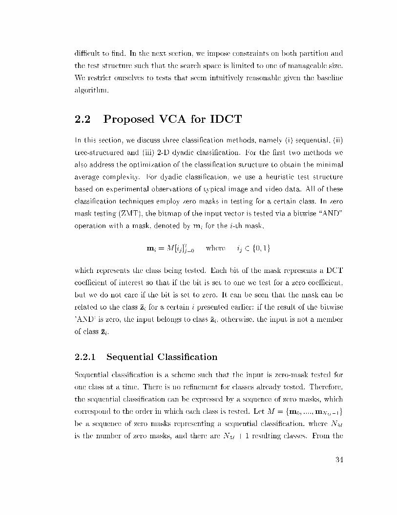
diÆcult to �nd. In the next section, we impose constraints on both partition and

the test structure such that the search space is limited to one of manageable size.

We restrict ourselves to tests that seem intuitively reasonable given the baseline

algorithm.

2.2 Proposed VCA for IDCT

In this section, we discuss three classi�cation methods, namely (i) sequential, (ii)

tree-structured and (iii) 2-D dyadic classi�cation. For the �rst two methods we

also address the optimization of the classi�cation structure to obtain the minimal

average complexity. For dyadic classi�cation, we use a heuristic test structure

based on experimental observations of typical image and video data. All of these

classi�cation techniques employ zero masks in testing for a certain class. In zero

mask testing (ZMT), the bitmap of the input vector is tested via a bitwise \AND"

operation with a mask, denoted by �mi for the i-th mask,

�mi =M [ij ]7j=0 where ij 2 f0; 1g

which represents the class being tested. Each bit of the mask represents a DCT

coeÆcient of interest so that if the bit is set to one we test for a zero coeÆcient,

but we do not care if the bit is set to zero. It can be seen that the mask can be

related to the class �zi for a certain i presented earlier: if the result of the bitwise

'AND' is zero, the input belongs to class �zi, otherwise, the input is not a member

of class �zi.

2.2.1 Sequential Classi�cation

Sequential classi�cation is a scheme such that the input is zero-mask tested for

one class at a time. There is no re�nement for classes already tested. Therefore,

the sequential classi�cation can be expressed by a sequence of zero masks, which

correspond to the order in which each class is tested. Let M = f �m0; ::::; �mNM�1gbe a sequence of zero masks representing a sequential classi�cation, where NM

is the number of zero masks, and there are NM + 1 resulting classes. From the

34

previous subsection, we know that �zi is a class tested by �mi. However, it is

possible that some primitive classes in �zi are also members of �zi�1 which will

be tested �rst. Therefore, the actual set of primitive classes tested at step i,

denoted by �di, is �zi � [i�1j=0�zj. The last class (default class) after the last test is

�dNM+1 = C8 � [NM�1j=0 �zj, where C8 = [255j=0�sj is the set of all primitive classes.

Without loss of generality, let us reuse the notation for the minimal complexity

reduced algorithm, A�i , for class

�di. Therefore, we can write the expression for

the average complexity of the sequential classi�cation IDCT as

Tseq =NM�1Xi=0

(c(ZMT )�(i+1)+c(A�i ))�Pd(i)+(c(ZMT )�NM+c(A�

NM+1))�Pd(NM+1)

(2.4)

where c(ZMT ) is the cost of zero masking test and Pd(i) is the probability of class

�di. Since the cost of ZMT is the same for every mask, the testing cost for the

i-th mask is (i+1) times the ZMT cost since there must be i+1 ZMT prior to the

i-th mask. The term outside the summation in (2.4) represents the cost for the

default class. Therefore, we can formalize the complexity minimization based on

sequential test as

Formulation 2 (Optimal Sequential Classi�cation VCA) The goal is to �nd

the optimal zero mask sequence M� such that the total average complexity is min-

imal. In other words, we want to minimize

T �seq = min

M2MTseq (2.5)

whereM is the set of all possible zero mask sequences M .

2.2.2 Greedy Optimization

The problem formulation is fairly straightforward but in order to obtain the op-

timal solution, exhaustive search is unavoidable. One can view the exhaustive

search as a tree search in which the tree grows to all possible directions. The time

required for exhaustive search can be reduced by using the knowledge of the re-

dundancy between zero masks, i.e., the fact that, as mentioned earlier, set �zi and

�zj for given i and j may have a non-empty intersection. Thus, the path to a node

35

that corresponds to a subset of previous nodes can be omitted. Yet, it is still time

consuming to �nd the optimal solution and it may not be practical to look for it

when the size of the input vector is larger than 8. Finding suboptimal solutions

is thus a more attractive alternative. Algorithms such as the M-algorithm [95], in

which only M best paths are kept at each iteration, can be used. In this work, we

use an even simpler and faster approach than the M-algorithm.

We use a greedy approach, in which the class that gives maximal complexity

savings is tested �rst, and then the classes with less computational saving are

tested later, until no further savings can be achieved from the classi�cation, i.e.,

the savings from using a RIDCT is outweighed by the cost of testing. When

that point is reached the default algorithm is applied to the remaining (untested)

classes. Prior to performing a greedy optimization, the statistics of each class �si,

for all i are assumed to be known. Let Ps(i) denote the probability of a primitive

class �si. Let us de�ne the complexity savings of reduced algorithm A�i of class �zi

by ~ci = c(A8) � c(A�i ), where A8 represents the baseline algorithm. The Greedy

approach can be described as follows.

Algorithm 1 (Greedy Optimization)

Step 1: Assume known probabilities of all primitive classes, Ps(i); 8 i. Initial-ize the list of sequential tests M as an empty set. Set NM = 0.

Step 2: Find class i such that the incremental complexity savings is maxi-

mal, i.e., i� = argmax �mi =2NM�~ci where �~ci = ~ci � Pd(i) � c(ZMT ) � Puntested and

Puntested = PrfC8 � [NM�1i=0 dig.

Step 3: If �~ci� > 0 put �mi as the last element in M and increment NM by 1.

Otherwise, stop.

Step 4: If NM = 256, stop. Otherwise go to Step 2.

The calculation of Pd(j) in Step 4 has to take into account the redundancy of

previous zero mask tests by excluding the probability of the primitive classes that

have already been tested.

36

2.2.3 Tree-structured classi�cation (TSC)

In this subsection, we propose an alternative to sequential classi�cation. Unlike

sequential classi�cation where the tested classes are not re�ned or tested again,

the tree-structured classi�cation (TSC) allows hierarchical testing in which tested

classes can be further classi�ed for more accurate positions of zeros, which also

implies better RIDCTs. The key idea of TSC is to exploit the structure of the

baseline algorithm in classi�cation. Consider the baseline full version of the IDCT

algorithm we have chosen, which is shown in Fig. 1.3(b). In this IDCT algorithm

there are three stages of operations, each of which involves 2, 4 and 8 input

coeÆcients, respectively. This tree-like structure provides a natural way of hier-

archically classifying the data, going from coarse to �ne classi�cation, i.e., ZMTs

that test a larger group of coeÆcients and then smaller and smaller groups.

In Fig. 1.3(b), let us consider the issue of grouping �rst. Needless to say, when

all 8 coeÆcients are zero, all branches up to stage 3 can be pruned. Given that 4

out of 8 coeÆcients are zero, the two scenarios that give the largest reductions in

complexity will correspond to the cases when (X7; X1; X3; X5) or (X0; X4; X6; X2)

are all zero, since branches of zero coeÆcients in stage 1 and stage 2 can be

pruned. For the case when 2 coeÆcients are zero, (X2; X6), (X1; X7), (X3; X5)

and (X0; X4) give the four minimal complexity RIDCTs since the corresponding

operations of these 4 pairs in stage 1 can be pruned. When only one coeÆcient

of those pairs is zero, stage 1 operation can be partially pruned. From these, we

can �nd, for the case when any number of coeÆcients is zero, the grouping with

maximal complexity reduction which is a combination of the above 4, 2 and 1

coeÆcients.

As far as the test structure is concerned, in order to achieve the above group-

ing with maximal eÆciency regardless of the statistics of the input (assuming a

uniform distribution of the input classes), groups with lower complexity RIDCT

should be tested before groups with larger complexity RIDCT. In this case, the

all-zero input class must be tested �rst. Then the two 4-zero classes, the four

2-zero classes and �nally the eight 1-zero classes are tested in succession. This

hierarchical testing results in at most 15 tests before a certain class can be iden-

ti�ed. An example of pseudo code for testing 2 coeÆcients at the second stage of

37

the upper 4 branches of Figure 1.3(b) is shown in Figure 2.1.

if(X2==0 and X6==0)

z0 = z3 = y0z1 = z2 = y1

/********* save computation for y2 and y3 ***********/

else if(X0==0 and X4==0)

z0 = y3, z1 = y2z2 = �y2, z3 = �y3

/********* save computation for y0 and y1 ***********/

else z0 = y0 + y3z1 = y1 + y2z2 = y1 � y2z3 = y0 � y3

/********* performing full version for this part ***********/

Figure 2.1: TSC pseudo code for testing upper 4 branches of Fig. 1.3 (b) in stage

2.

This TSC is illustrated in Figs. 2.2 and 2.3. For simplicity in explanation,

we denote Ci0i1i2i3i4i5i6i7 as a class of input obtained from TSC. The classi�cation

information ij indicates the following.

ij =

8>>>>>><>>>>>>:

Ek k 2 f1; 2; :::g means that at least one of coeÆcients indexed

with a given Ek is nonzero

0; 1 means that xj is \known" to be zero or nonzero

U means xj can be either zero or nonzero (unknown)

As an example, CE1UE20E10E2U means that at least one of fx0; x4g and one of

fx2; x6g must be nonzero, x1 and x7 are unknown, and x3 and x5 are both known

to be zeros. Thus, in order to perform IDCT correctly an RIDCT must assume

that all coeÆcients except x3 and x5 are zero. Note that the class in the example

above can be represented as Zc[01110111] \ Zc[11011101] \ Z[11101011], whereZc[:] is a complement of set Z[:]. The newly introduced notation is obviously more

concise.

Fig. 2.2 illustrates the tree-structured classi�cation of size 8 DCT coeÆcients.

Each node represents a class with some knowledge about the positions of zero

coeÆcients. Descendents of each node are the results of �ner classi�cations, i.e.,

they contain more information about zero coeÆcients than their parent nodes. For

38

CUUUUUUUU

C00000000 CE1E1E1E1E1E1E1E1

C0E10E10E10E1 CE1E2E1E2E1E2E1E2CE10E10E10E10

all-zero test

quadruplet test

⊗

Figure 2.2: TSC diagram showing zero information of classes after all-zero test

and 4-zero tests.

simplicity, in the �gure the tree is grown to the level of 4-zero classes only. Finer

classi�cations are shown in Fig. 2.3 where 2-zero and 1-zero tests are performed.

It can be veri�ed that a total of 256 primitive classes can be obtained with this

TSC if the tree is constructed from all-zero level down to 1-zero test level, i.e.,

combining Fig. 2.2 and 2.3.

Every nodes of the tree in Fig. 2.2 and 2.3 has an associated RIDCTs. The

RIDCTs for those classes are based on pruning only operations that involve co-

eÆcients that are known to be zero. Thus, we cannot prune operations involving

coeÆcient labeled with U or Ek unless we are willing to have a non-exact IDCT.

2.2.4 Optimal Tree-structured Classi�cation (OTSC)

Note that in Section 2.2.3, we outlined the classes that are induced by testing in

a hierarchical manner, starting with tests on 4 coeÆcients and continuing with

two and then one coeÆcient. At each node, in order to classify to 3 classes,

two logical operations must be performed. For example, class CE1E1E1E1can be

classi�ed to C0E10E1and CE1UE1U using AND logic between the input bitmap and

the mask M [1010]: if the result is zero, the input belongs to C0U0U , otherwise it

belongs to CE1UE1U . Then CE1UE1U is further classi�ed to CE10E10 and CE1E2E1E2

by performing an AND of the input bitmap withM [0101]: if the result is zero, the

39

CE1E1E1E1

C0E10E1 CE10E10

CE1E3E1E3

C0001

C0100

C0101

C0010

C1000

C1010

CE10E11

CE11E10

CE11E11

C0E31E3

C1E30E3

C1E31E3

⊗

Figure 2.3: TSC diagram showing zero information of classes after 2-zero test and

1-zero tests. The most right-handed class after 2-zero test is further classi�ed into

9 classes which are tensor products of descendent classes shown, i.e., A B =

f(Ai \ Bj)g8 i;j where A = fAig; B = fBig. Therefore, the number of leaves is

3+3+(3x3) = 15.

input belongs to CE10E10, otherwise it belongs to CE1E2E1E2. However, the order

in which M [0101] and M [1010] are applied can be switched, and the resulting

3 classes can still be obtained. However, the complexities of both orderings are

di�erent when the frequency of occurence of the resulting classes is taken into

account. For example, in the above example, if class CE10E10 occurs more often

than C0E10E1, then regardless of RIDCTs complexity2 it is better to apply the

mask M [0101] before M [1010].

Therefore, for optimal TSC tests, ordering has to be carefully chosen. Fur-

thermore, we allow more freedom to perform only one logic operation at a node

to classify only 2 classes, e.g., in the above example, we can choose to have only

the second test performed on CE1E1E1E1to get CE10E10 and CUE1UE1

. Thus, the

goal of our optimization procedure is to �nd the best classi�cation, that is, to

determine (i) the best order in which to apply the tests and (ii) which tests it is

worth performing (in the sense of reducing the average complexity).

In Figs. 2.4, we show the possible choices for testing 4 coeÆcients. We denote

the two logic comparisons by A and B. In the �gure there are �ve possible choices

which are A-B, B-A, A only, B only and no-test. Each choice results in di�erent

classi�cations except A-B and B-A which have the same �nal result. Given the

2In our work, the RIDCTs complexity has to be taken into account in order to obtain minimaltotal complexity.

40

CE1E1E1E1

CE1UE1UC0E10E1 CE10E10 CUE1UE1

C0E10E1 CE10E10 CE1E2E1E2

&0101 == 0 ?&1010 == 0 ?

&0101 == 0 ? &1010 == 0 ?

A B

B A

Figure 2.4: Diagram showing possible choices for classi�cation at level 2 where A,

B represent testing with M [1010] and M [0101], respectively.

CUUUU

CE1UE1UC0U0U CU0U0 CUE1UE1

C0U0U CE10E10 CE1E2E1E2

&0101 == 0 ?&1010 == 0 ?

&0101 == 0 ? &1010 == 0 ?

A B

B A

CU0U0 C0E10E1 CE2E1E2E1

Figure 2.5: Another diagram when the result from level 1 is di�erent.

statistics of the input, we can then compare the complexity including the test to

�nd the best choice on the average sense. The complexities of the �ve choices as

shown in Fig. 2.4 are

TA�B = c(SA)PE1E1E1E1+ c(SB)PE1UE1U +

c(A�0101)P0E10E1

+ c(A�1010)PE10E10 + c(A�

1111)PE1E2E1E2

TB�A = c(SB)PE1E1E1E1+ c(SA)PUE1UE1

+

c(A�0101)P0E10E1

+ c(A�1010)PE10E10 + c(A�

1111)PE1E2E1E2

TA�only = c(SA)PE1E1E1E1+

c(A�0101)P0E10E1

+ c(A�1111)PE1UE1U

TB�only = c(SB)PE1E1E1E1+

c(A�1010)PE10E10 + c(A�

1111)PUE1UE1

41

Tno�test = c(A�1111)PE1E1E1E1

We can perform the comparison of these 5 choices at all level of testing i.e.,

all-zero, 4-zero, 2-zero and 1-zero test. In the case, where A-only, B-only or no-

test are chosen in the previous level of zero testing, the current level will start

with a class which no information has been obtained, see Fig.2.5. From the TSC

tree in Fig. 2.2 and 2.3 we compare all possible combinations of 5 choices in every

node to �nd the test structure with minimal complexity.

For consistency with previous formalization, let H be rede�ned as a set of

choices at each node in Fig. 2.2 and 2.3.

H = fh0; h1; fh2i ; h34i; h34i+1; h34i+2; h

34i+3g3i=0g

where hli 2 fA� B; B� A; A� only; B � only; no � testg is the choice selected at

level l and node i. There are 4 levels corresponding to all-zero, 4-zero, 2-zero and

1-zero test. If the previous level performs classi�cation with less than 3 classes,

not all of next level choices are available. For example, if h1 = A� only, the

resulting classi�cation is fCE10E10E10E10; CUE2UE2UE2UE2g then h21 has no value be-

cause the class C0E10E10E10E1is not classi�ed but included in CUE2UE2UE2UE2

. Also

h34; h35; h

36; h

37 have no values either. Thus our optimization goal can be formalized

as

Formulation 3 (Optimal Tree-Structured Classi�cation VCA) The goal is

to �nd H� from all possible combinations H such that the overall complexity is

minimal i.e., we minimize the average complexity

T �TSC(binary)(P ) = min

H2HTTSC(binary)(H;P ) (2.6)

for a given statistics of input classes.

Let H� represent an optimized TSC (OTSC) algorithm which can be found

by searching overall possible test structure space, H, satisfying the above binaryTSC framework.

42

2.2.5 Computation of 2-D IDCT

As mentioned earlier, there are several approaches to classify a 2-D DCT input

block using the previously proposed algorithms. For example, we can directly test

the coeÆcients in a 2-D block as in [60]. We can also apply OTSC to each row of

input in the row-wise 1-D IDCT and then apply the OTSC for each column of the

row-wise IDCT output in the column-wise 1-D IDCT. For simplicity, we choose

to perform the latter (separable 2-D IDCT). Note that, we can have di�erent

OTSCs for di�erent row and column positions but the overhead of caching di�erent

functions in the software implementation outweighs the complexity reduction of

having more OTSCs for di�erent row/column statistics. Thus we use the same

algorithm for all rows/columns.

X X X X XX X XX

X

X

X

X

X

X

X X X X XX X XX

X

X

X

X

X

X X XX X X X X

X X X X X

X X X X X

X X XX X X X X

DCT

rowwise

Figure 2.6: Content of bitmap after �rst (row-wise) 1-D IDCT where 'x' represents

nonzero coeÆcient.

Except for the 2-D dyadic classi�cation in Section 2.2.6, the TSC and se-

quential classi�cation schemes require re-classi�cation for the intermediate result

between the 1-D separable IDCTs. After the rowwise 1-D IDCT, the input to

the columnwise 1-D IDCT has to be classi�ed again. The bitmap for the second

IDCT can be approximated very accurately from the �rst bitmap as shown in

Figure 2.6. The approximation relies on the fact that if at least one frequency

component is nonzero it is more likely that all the outputs from the IDCT (i.e.

the result of applying the IDCT to the row or column) will be all di�erent from

zero. There are very unlikely cases where magnitude cancellation occurs at some

output points and the output is zero even though there were non-zero inputs but

we ignore these cases. The complexity savings from this bitmap implementation

is about 5% over direct coeÆcient testing.

43

2.2.6 2-D Dyadic Classi�cation

In the above proposed classi�cation schemes, i.e., Sequential Classi�cation and

TSC, 1-D IDCT is the target the classi�cations are applied on. They both can

be extended to 2-D classi�cation but the complexity is also increased and the

optimization process may become impractical. Therefore, we propose an alterna-

tive classi�cation in which a block of 2-D DCT coeÆcients is classi�ed instead of

classifying each row/column separately. We propose 2-D dyadic classi�cation in

which an NxN DCT block is classi�ed into all-zero, DC-only, low-2x2, low-4x4,

low-8x8, .... , N2xN

2, and full-NxN classes. For each of these classes, a corre-

sponding 1-D RIDCT is applied along the nonzero rows and then all columns.

The testing order follows the above list. The reason behind this classi�cation is

from the fact that in typical image high frequency components are more likely to

be quantized to zero. Figure 2.7 shows how the classi�cation works.

INPUT

KNKN/2

K1

KN/2

all-zero

K2

Figure 2.7: Dyadic classi�cation scheme. A DCT input of size NxN is classi�ed

into all-zero, DC-only (K1), low-2x2 (K2),..., low-N2xN

2(KN=2), and full-NxN

(KN) classes.

When the baseline algorithm has a recursive structure in the sense that larger

size IDCT computation consists of smaller sizes IDCT computations, we can ex-

press the complexity of the RIDCTs, accordingly. For example, the Chen,Smith

&Fralick [28] or the Vetterli-Ligtenberg [29] (Fig. 1.3) algorithms can be decom-

posed to a normal half-size IDCT (type II) and a half-size IDCT of type IV [24]

and the normal half-size IDCT can be further decomposed and so on. Therefore,

it is equivalent to having smaller size IDCTs as the RIDCTs. The complexity

44

for each class tested by dyadic classi�cation on an NxN DCT block can then be

written as

c(A�i ) = (N +

N

2log2 N�i+1)KN=2log2 N�i+1 (2.7)

for class i = 1; 2; :::; log2N + 1 where KN is the complexity of DCT/IDCT of

size N and when i = 0, c(A�0) = 0 for all-zero block. The term that multiplies

K represents the number of rows and columns on which 1-D reduced IDCT is

performed. Here, we use a separable reduced size 1-D IDCT to perform 2-D

IDCT. The reduced rowwise transform is performed only for rows with nonzero

coeÆcients. Then the reduced columnwise transform is applied to all columns. In

terms of classi�cation structure, it can be seen that, unlike the greedy approach,

the order of classi�cation (or threshold testing) is �xed and the closed form com-

plexity expressions of the reduced algorithms are known. Let Bi denote class i

input. Thus, the complexity of Bi can be written as

Tdyadic(Bi) = c(A�i ) + i � Tdtest (2.8)

where Tdtest represents the testing cost (2-D zero mask or series of 1-D zero mask

tests). For simplicity, we assume that Tdtest is constant for all classes. From (2.8),

the average complexity can be expressed as

�Tdyadic =log2 N+1X

i=1

(Tdyadic(Bi) � Pr(Bi) (2.9)

where Pr(Bi) is the probability of class Bi which is a function of QP, �2 and N .

2.3 Results

In our experiments we implement a real software image decoder using the OTSC.

For sequential testing, we only implement a greedy optimization based on an

image model.

The main problem now is obtaining accurate models for the costs of the opera-

tions used in ZMT, and RIDCT, such as addition, multiplication, shift, OR, NOT,

45

Table 2.1: Weight for di�erent logical operations.

Operation Weight

Addition 1

Binary Shift 1

Binary OR 1

Multiplicatio 3

Conditional Branching 5

IF, etc. While this may be relatively straightforward in hardware implementa-

tions or for assembly language level programming, it is more complicated if we

use a high level programming language, since the e�ect of memory accesses, size

of the code and so forth are more diÆcult to characterize. This problem is very

diÆcult to solve since it highly depends on compiler and machine architecture. To

obtain more accurate estimates one could resort to an assembly language imple-

mentation or to measuring the average time complexity for each of the possible

classi�cation trees directly. This latter approach would clearly be too complex

and still would not guarantee an exact cost measure, since many di�erent factors

a�ect the runtime performance.

For the sake of practicality, we just use a set of approximated weights for the

operations involved. By feeding these approximated parameters into our search

algorithms we can get a fairly accurate approximation to the optimal solution.

We have used a Sun Sparcstation 5 running Solaris 2.5 with the gcc compiler, and

Pentium 450 MHz running WindowNT 4.0 with Visual C++ compiler. We use

the assessment in Table 2.1 for each operation [96].

Note that one IF statement consists of comparing to zero and a jump operation.

One more thing to be considered here is memory access. Whenever one variable

is involved in an operation, there is either a read-in or write-out time. However,

since this memory access can be highly optimized using an optimization option by

the compiler, we do not take that into account. We emphasize this issue because

our costs are only approximated and very machine dependent. Hence, we do not

guarantee that the result of the OTSC will be the same for all environments.

46

2.3.1 Results Based on Image Model

In this section we assume that the image characteristic to be tested follows the

model presented in Section 1.6 (assuming INTER-frame coding). Therefore, given

that the model parameter is known, the probability of X(u,v) being zero (pz(u; v))

can also be computed. Thus, we can obtain the average complexity of any algo-

rithms. We perform our experiments on di�erent values of the model parameter

and the quantization parameter.

First we will show the results of both the greedy and OTSC compared to that of

an ideal algorithm in which the classi�cation comes for free. That is, we assume

we know the exact position of the zeros in the input so that all corresponding

operations can be pruned without any testing overhead. Fig. 2.8 shows the number

of additions and multiplications as functions of the quantization parameter (QP)

of the Greedy and OTSC compared to the ideal case. In addition to using the

Vetterli-Ligtenberg algorithm (Fig. 1.3 (b)) as the baseline algorithm, we show

the ideal case when direct matrix multiplication method is used instead. It can

be seen that in all cases the ideal direct matrix multiplication is inferior to the

ideal fast search based algorithm.

0 5 10 15 20 25 300

0.1

0.2

0.3

0.4

0.5

0.6

0.7

0.8

0.9

1

QP

Normalized additions

OTSC

Greedy

Ideal Fast

Ideal Direct

:σ2 = 700

:σ2 = 100

(a)

10 12 14 16 18 20 22 24 26 28 300

0.1

0.2

0.3

0.4

0.5

0.6

0.7

0.8

0.9

1

QP

Normalized Multiplications

OTSC

Greedy

Ideal Fast

Ideal Direct

:σ2 = 700

:σ2 = 100

(b)

Figure 2.8: Number of additions (a) and the number of multiplications (b) needed

for �2 = 100 and 700, using OTSC ('solid'), Greedy ('dashed'), Ideal fast IDCT

('dashed-dotted'), and Ideal matrix multiplication ('light-solid'). The OTSC and

Greedy are optimized for each QP.

47

0 5 10 15 20 25 300

0.2

0.4

0.6

0.8

1

QP

Total Normalized Complexity

OTSC

Greedy

:σ2 = 700

:σ2 = 100

(a)

0 5 10 15 20 25 300

1

2

3

4

5

6

7x 10

5

QP

Number of Tests

OTSC

Greedy

:σ2 = 700

:σ2 = 100

(b)

Figure 2.9: Total complexity (a) and the number of tests (b) needed for �2 = 100

and 700 using OTSC ('solid') and greedy ('dashed') algorithms.

One can also observe that in terms of number of additions and multiplications,

the OTSC requires less operations than the Greedy approach. This is because

the ability to re�ne the tests within OTSC allows better classi�cation than the

greedy approach. The result of the OTSC in terms of number of additions and

multiplications is very close to the ideal case at high quantization and moves

away from the ideal as �ner quantization is used, see Fig. 2.8. This can be easily

explained since in the low rate region most of the quantized DCTs are zero and

therefore the zero tests become very eÆcient. On the other hand, at high rate

there are less zero DCTs, thus resulting in a waste of zero mask test computations.

Also in Fig. 2.9, the complexity reduction of the OTSC comes at the price of

using numerous tests (as can be seen in Fig. 2.9 (b)), which essentially makes

the algorithm very machine-dependent, i.e., the total cost could vary a lot from

machine to machine. On the other hand, the number of tests (bit map testings)

required by the greedy approach is much less than OTSC, thus compensating its

larger number of multiplications and additions and resulting in similar overall

complexity.

We emphasize that the greedy approach performs very close to the OTSC in

terms of total complexity while the number of tests is much less. Therefore, it

can be accurately used as an indicator of the complexity of the OTSC at various

48

block sizes with much less optimization e�ort. We show the distortion-complexity

and rate-complexity (R-C) performance of di�erent IDCT algorithms at di�erent

QP and block sizes in Figure 2.10 (a) and (b), respectively.

0 5 10 15

x 106

0

10

20

30

40

50

60

70

80Complexity−Distortion for σ2 = 100

Complexity per 64 pixels

Dis

tort

ion

(mse

)

:Dyadic Ideal

:Greedy

:DCT 16x16

:DCT 8x8

:DCT 4x4

(a)

0 5 10 15

x 106

0

0.2

0.4

0.6

0.8

1

1.2

1.4Rate−Complexity for σ2=100


Rat

e (b

it/pi

xel)

:Dyadic Ideal

:Greedy

:DCT 16x16

:DCT 8x8

:DCT 4x4

(b)

Figure 2.10: (a) Complexity-distortion and (b) Rate-complexity curves for dif-

ferent algorithms, i.e., greedy ('dotted') and 2-D dyadic ('dashed'), for DCT size

16x16 ('x'), 8x8 ('o') and 4x4 ('*') at �2 = 100. The complexity unit is weighted

operations per 64 pixels.

From Figure 2.10 (a), we can see that, for a given distortion, which block size

gives the least complexity depends on �2 and QP . It can be seen that at low

distortion, smaller block size is cheaper than large block size, whereas the reverse

is true at high distortion. From Figure 2.10 (b), it can be seen that as rate becomes

small, the complexity di�erence between each block size becomes smaller as well.

Therefore, the conclusion is that using large block sizes at low rates results in

comparable complexity and distortion performances to using smaller block size.

The C-D and R-C results of 2-D dyadic are also shown in Fig. 2.10 (a) and

(b), respectively. At this point, we can also compare the 2-D dyadic testing to

the greedy approach. We can see that at high rate the dyadic test requires higher

complexity than the greedy algorithm because the classi�cation is coarser for

the higher frequency components. However, at lower rate the complexity of the

dyadic test is lower since there are fewer tests in the dyadic test and the test is

performed on a whole 2-D block, instead of each row or column, thus resulting in

more eÆcient classi�cation cost. In fact, the 2-D test can be performed eÆciently

49

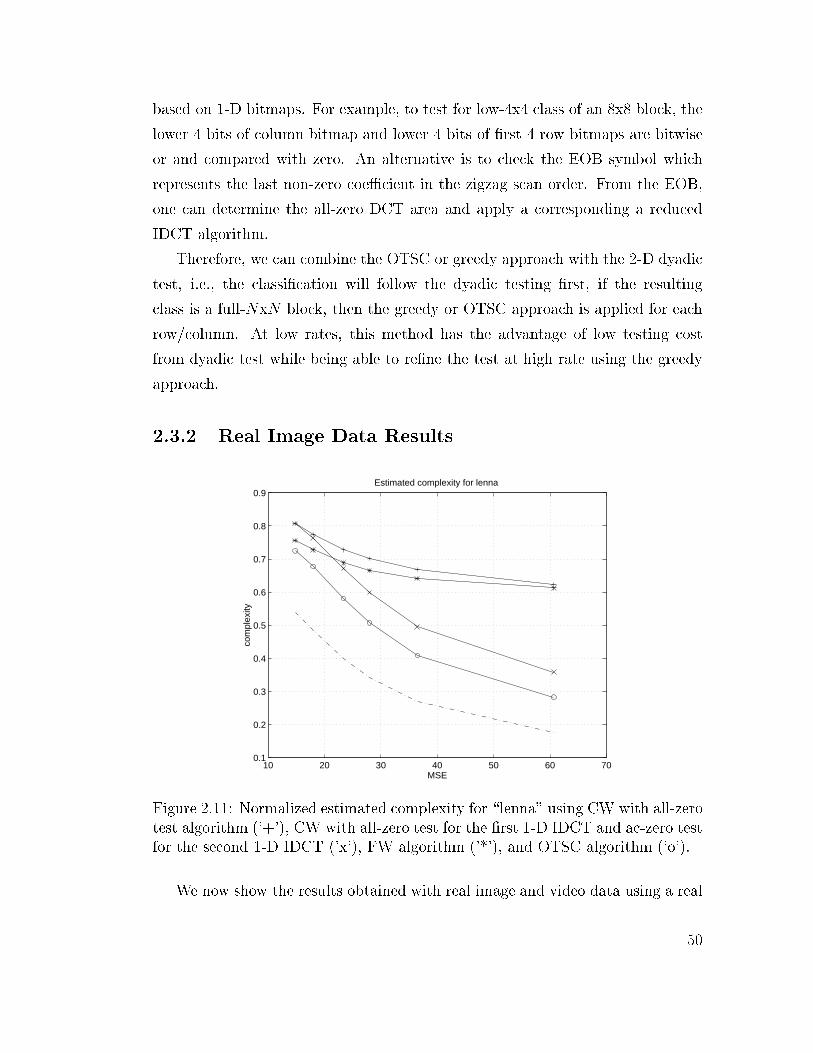
based on 1-D bitmaps. For example, to test for low-4x4 class of an 8x8 block, the

lower 4 bits of column bitmap and lower 4 bits of �rst 4 row bitmaps are bitwise

or and compared with zero. An alternative is to check the EOB symbol which

represents the last non-zero coeÆcient in the zigzag scan order. From the EOB,

one can determine the all-zero DCT area and apply a corresponding a reduced

IDCT algorithm.

Therefore, we can combine the OTSC or greedy approach with the 2-D dyadic

test, i.e., the classi�cation will follow the dyadic testing �rst, if the resulting

class is a full-NxN block, then the greedy or OTSC approach is applied for each

row/column. At low rates, this method has the advantage of low testing cost

from dyadic test while being able to re�ne the test at high rate using the greedy

approach.

2.3.2 Real Image Data Results

10 20 30 40 50 60 700.1

0.2

0.3

0.4

0.5

0.6

0.7

0.8

0.9

MSE

com

plex

ity

Estimated complexity for lenna

Figure 2.11: Normalized estimated complexity for \lenna" using CW with all-zero

test algorithm ('+'), CW with all-zero test for the �rst 1-D IDCT and ac-zero test

for the second 1-D IDCT ('x'), FW algorithm ('*'), and OTSC algorithm ('o').

We now show the results obtained with real image and video data using a real

50

10 20 30 40 50 60 700.35

0.4

0.45

0.5

0.55

0.6

0.65

0.7

0.75

0.8

0.85

MSE

com

plex

ity

Actual experimental time for lenna (algorithm time)

Figure 2.12: Normalized actual time complexity (only IDCT algorithm part) for

\lenna" using CW with all-zero test algorithm ('+'), CW with all-zero test for

the �rst 1-D IDCT and ac-zero test for the second 1-D IDCT ('x'), FW algorithm

('*'), and OTSC algorithm ('o').

image and video decoder. First we show the result of OTSC on image data (see

Fig. 2.11). The results show the estimated complexity comparison between (i)

IDCT based on our proposed method (OTSC), (ii) the baseline algorithm (CW)

with all-zero test, (iii) the baseline (CW) algorithm with all-zero test for the �rst

1-D IDCT and AC-zero test for the second 1-D IDCT (since after the �rst 1-D

IDCT, it is more likely for typical images that only the DC coeÆcient in the

1D vector is non-zero) and (iv) the FW method, for various mean squared error

values obtained by changing the quantization parameter. We use the example

quantization table from the JPEG standard [1]. All the values are normalized by

the complexity of the baseline algorithm without all-zero test. Next, the actual

implementation times are shown for IDCT algorithm part (Fig. 2.12) and total

decoding time (Fig. 2.13), which includes the time for read-in and write-out of the

input data. Also shown in Fig. 2.14 is the mismatch case, i.e., we use the IDCT

algorithm optimized for a speci�c image at a certain quality factor for a di�erent

image and/or quality factor.

51

10 20 30 40 50 60 700.55

0.6

0.65

0.7

0.75

0.8

0.85

0.9

MSE

com

plex

ity

Actual experimental time for lenna (total decoding time)

Figure 2.13: Normalized actual time complexity (total decoding time) for \lenna"

using CW with all-zero test algorithm ('+'), CW with all-zero test for the �rst

1-D IDCT and ac-zero test for the second 1-D IDCT ('x'), FW algorithm ('*'),

OTSC algorithm ('o'). OTSC for lenna at MSE 14.79 ('{'), and OTSC for lenna

at MSE 60.21 ('-.').

Our proposed method (OTSC algorithm) achieves up to 50% complexity re-

duction for the IDCT part. When there is a mismatch between the statistics of

the training data and those of the actual data being processed, the performance

can be degraded. Another source of mismatch comes from the assessment for the

cost of each operation, which must be precise enough to maintain the consistency

between the estimated complexity and the actual complexity. As seen for both

experimental results, even with mismatches, the optimized algorithm is a little

bit inferior because of the lack of an exact model for the complexity. However, if

our estimation for cost of operations is precise enough, a conclusion drawn from

the result when applying optimized IDCT algorithm for \lenna" with MSE 60.21

could be that the degradation for using an algorithm optimized for a higher MSE

(which overestimates the number of zeros) is less than the degradation for an al-

gorithm optimized for a lower MSE (which underestimates the number of zeros).

This may not be true for other types of images. Also it has to be pointed out that

52

50 100 150 200 250 300 3500.7

0.75

0.8

0.85

0.9

0.95

1

MSE

norm

aliz

ed c

ompl

exity

Actual Experimented time (total decoding time)

Figure 2.14: Normalized actual time complexity (total decoding time) for baboon

image using CW with all-zero test algorithm ('+'), CW with all-zero test for the

�rst 1-D IDCT and ac-zero test for the second 1-D IDCT ('x') , FW algorithm

('*'), OTSC algorithm ('o'), and OTSC for lenna with MSE 14.79 ('{')

our current implementation has concentrated mostly on the issue of structuring

the tests, and thus uses a very simple programming style. Our goal at this stage

was to implement all the algorithms with a similar style so that a fair comparison

is possible.

The results of the combined 2-D dyadic and OTSC IDCT are shown in Fig. 2.15

using TMN's codec [58] and coding 249 frames of the \Foreman" sequence at

di�erent target bit rates. The inverse quantization complexity is also considered

since there is an overhead cost of bitmap generation for both OTSC and dyadic.

It can be seen from Fig. 2.15 that the combined dyadic-OTSC gets an extra 6-9%

complexity reduction from the OTSC. An explanation is that the 2-D classi�cation

is cheaper than separate 1-D classi�cation, if it matches the statistics of the data

well. In typical image and video data, nonzero coeÆcients tend to cluster around

DC component. That is why we observe extra speedup using dyadic classi�cation.

We now discuss the issue of statistical estimation. One scenario to obtain the

statistics for the proposed VCA IDCTs in a practical encoding system would be to

53

0.45 0.5 0.55 0.6 0.65 0.727

27.5

28

28.5

29

29.5

30

30.5

31

31.5IDCT + inverse quantization complexity results of "foreman"

Normalized complexity

PS

NR

50 Kbps

40 Kbps

30 Kbps

20 Kbps

OTSCDyadic+OTSC

Figure 2.15: The complexity (CPU clock cycle) of the IDCT + Inv. Quant.

normalized by the original algorithm in TMN at various PSNRs (di�erent target

bit rates) using OTSC ('4') and combined dyadic-OTSC ('*').

have the encoder send side information about the optimized tree-structure zero-

test IDCT algorithm to the decoder along with the data, such that the decoder

can do the IDCT operation with the minimum complexity. However, this comes

with the price of bit rate overhead. As an alternative, a tree-structured or greedy

optimization can be performed at the decoding end using the past statistics of

input data. This seems to be more compatible with the existing image and video

standards. However, there is an issue of run-time algorithm change. It is impos-

sible to compile the optimal IDCT at run-time. Therefore, instead of optimizing

the VCA on the y, a more practical way is to have a set of pre-optimized VCAs

that covers a wide range of image statistics at run-time and choose the one with

smallest complexity for the image being operated.

2.4 Distortion/decoding time tradeo�s

As we mentioned earlier for the scalability issue, one way to achieve IDCT com-

putational scalability is by changing QP at the encoder side. This can be applied

to the case where a limited complexity decoder is the major concern. The C-D

tradeo� will be addressed, i.e., within a given computational complexity at the

54

decoder, the encoder adjusts the quantization parameter such that the distortion

is minimized while satisfying the complexity constraint. Note that this requires

the encoder to have enough information about the operation at the decoder end

in order to change the QP accordingly.

As described in the previous section a VCA implementation of the IDCT can

be obtained given a \typical" set of input images. As is clear from the results, the

coarser the quantization the faster the decoder can run. Thus, a decoder based

on a VCA IDCT is inherently computationally scalable. Unlike the JPEG case in

which the quantization parameter is �xed for all blocks in a coded image, for video

encoding standards such as MPEG1-2 or H.261-3 the encoder can adjust its quan-

tization parameter on every macroblock in order to try to �nd the best picture

quality for a given bit budget. The same idea can be applied to a complexity-

distortion (C-D) framework where the encoder can control the decoding speed by

assigning to each block one out of several available quantizers (coarser quantizers

result in faster operation). The question then arises on how to optimally select

those quantization steps for a given decoding time budget. This leads to a formula-

tion where the encoder operates based on a complexity-distortion (C-D) tradeo�,

rather than on the traditional rate-distortion (R-D) tradeo�. As an application,

one could for instance store images to be downloaded by di�erent types of hosts

so that the slower hosts can access lower quality images, which can be decoded

more quickly. Similarly, the quality of the decoded images can be selected based

on the load of the shared host. The problem can be formalized as �nding the

quantizer assignment fj; igopt such that

Xj

Dj(i) is minimized whileXj

Tj(i)) < Tbudget;

where Tbudget is the total time (or complexity) budget, Dj(i) and Tj(i) are, respec-

tively, the distortion and decoding time when quantizer i is used for block j. The

problem can be solved using the well-known Lagrangian multiplier method [9]

fj; igopt = argminfj;ig

(Xj

Dj(i) + � �Xj

Tj(i)) (2.10)

55

where � � 0 is the Lagrange multiplier, which will have to be adjusted so that

the budget is met.

10 20 30 40 50 60 700.2

0.3

0.4

0.5

0.6

0.7

0.8

MSE

com

plex

ity

Estimated complexity/distortion curve

(a)

10 20 30 40 50 60 700.55

0.6

0.65

0.7

0.75

0.8

0.85

MSE

com

plex

ity

Experimental distortion/complexity curve

(b)

Figure 2.16: Distortion versus (a) estimated IDCT complexity (b) experimental

decoding time of \lenna" using �xed quantizer encoder and OTSC decoder ('o'),

Lagrange multiplier results ('x'), encoder follows Lagrange multiplier results but

decoder uses a single OTSC for MSE=60.66 ('*') and MSE=14.80 ('+'), respec-

tively.

Figs. 2.16 and 2.17 summarize our results. In this experiment, we design six

OTSC algorithms for six di�erent quantization parameters based on the statistics

of the test image. The OTSC design is based on the approach discussed in the

previous section. We then have the complexity and distortion for each block and

each quantizer, as required by the Lagrange optimization of (2.10). For a given

�, we �nd the quantizer that minimizes (2.10) for each block. Finally, we repeat

the minimization at di�erent values of � until the complexity constraint is met.

Therefore, the encoder applies di�erent quantizers for di�erent blocks according

to the optimization result. The quantizer information must also be sent to the

decoder for proper inverse quantization. At the decoder side, the OTSC algorithm

that corresponds to the quantizer selected for the block is used. However, in most

of the cases, having many OTSCs at the decoder results in excessive overhead. A

more practical approach is to have a single OTSC optimized for a single quantizer

and to use this OTSC for all blocks.

56

10 15 20 25 30 35 40 45 50 55 600.25

0.3

0.35

0.4

0.45

0.5

0.55

0.6

0.65

0.7

0.75

MSE

com

plex

ity

Comparison of complexity between comp./dist. and rate/dist.

(a)

10 15 20 25 30 35 40 45 50 55 600.2

0.3

0.4

0.5

0.6

0.7

0.8

0.9

1

MSE

rate

(bp

p)

Comparison of rate between comp./dist. and rate/dist.

(b)

Figure 2.17: (a) Complexity-Distortion curve obtained from C-D ('x') and R-D

('*') based optimization. (b) Rate-Distortion curve achieved when C-D ('x') and

R-D ('*') based optimization. The complexity is normalized by the complexity of

the baseline Vetterli-Ligtenberg algorithm.

Fig. 2.16 indicates that quantizer allocation for each block optimized for com-

plexity results in very signi�cant reductions in complexity. As expected, the C-D

allocation outperforms the other methods. Note that in Fig. 2.16 (a) we compare

the C-D allocation when multiple quantization-dependent algorithms are used

and when a single algorithm is used (OTSC optimized for �ne quantizer or coarse

quantizer). When a coarse quantizer is used the performance is very close to that

of the multiple algorithm approach. This result is consistent with the previous

result in Fig. 2.13 where we can use an OTSC optimized for a coarse quantizer for

blocks coded with �ner quantization with only small degradation in C-D perfor-

mance. For the actual decoding tests we thus use a single algorithm. Each point

in the C-D optimized curves is obtained with a given parameter �.

One may argue that the complexity can be controlled via rate control since in

general, the quantizer is determined by bit budget. If the bit budget is small, a

coarse quantizer will be used, which in turn results in more DCT coeÆcients being

set to zero, so that decoder with VCA IDCT will be faster. However, Figs. 2.17 (a)

and (b) demonstrate how a complexity driven quantizer allocation results in better

C-D performance than its rate driven counterpart. Even though C-D and R-D

curves from both C-D based and R-D based optimization are close together, as

57

expected better performance can be observed when the correct budget constraint

parameter is used. However, we may also use a rate budget constraint instead of

a complexity constraint to obtain sub-optimal C-D performance.

2.5 Rate-Complexity-Distortion Quadtree Opti-

mization

There are only a few works addressing the rate-complexity-distortion tradeo�s.

Among those are [22] and [23] in which the complexity is considered as a factor

to determine the R-D performance, and can be varied by changing the size of

the block transform. In [23], the convexity of the R-D-C curve of Gauss-Markov

sources is proved. Furthermore, in [23] the C-D comparison for a given rate

between KLT and DCT is shown. An interesting conclusion can be drawn that

with this particular source the C-D curve of the DCT is better. However, in

these works the complexity is not input-dependent, i.e., it considers the worst-

case scenario which implies the complexity is a function of the block size. If we use

the variable complexity approaches proposed in the previous sections, it can be

seen that the C-D relation also follows a similar tradeo� as R-D when QP changes

(see Figure 2.10(a)) whereas (see Figure 2.10(b)) the R-C have the tradeo� when

the block size, not QP, varies. It is true because when the block size is larger, the

complexity required for block transform is also larger while the rate is smaller as a

result of the transform coding gain, and vice versa. However, since the number of

available block sizes is limited, in order to obtain a convex hull of the R-C curve,

the Lagrange multiplier method can be used as it is in R-D applications [9]. In

[97] and [21], quadtree-based coding is used for better R-D performance by using

a di�erent block size for di�erent regions and types of inputs. In [21], the R-D

optimization criterion is used with the optimal tree pruning algorithm [98]. The

optimization already incorporates the fact that the encoder has to send the block

size information to the decoder.

In this section, we present a more general R-C-D tradeo� based on the La-

grange multiplier technique, which incorporates the selection of QP and block size.

We will �rst formalize a problem similar to the optimal quadtree based coding of

58

1

001

0

1

010

1

0

1

000

0

Figure 2.18: Quadtree structures of four 16x16 regions and the corresponding

representative bits.

[21], with an additional constraint on the complexity. Then the QP as well as the

block size are optimally selected for each block of the image or the video frame.

The complexity constraint is the target total decoding time at the decoder.

We use the same notations as [21]. Based on Figure 2.18, let Xn;i denote the

i-th DCT block at level n. As in the �gure, the leaves (smallest blocks) correspond

to a block size of 4x4, the middle nodes represent 8x8 blocks and the root of each

tree corresponds to block size of 16x16. Let n = 0; 1; 2 represent blocks of size

4x4, 8x8 and 16x16, respectively. The scheme can be generalized to smaller block

size (i.e., 1x1 block) or larger block size such that level n corresponds to block

size 2nx2n. However, given the limitation on computation, we use only 3 block

sizes. The side information needed to be sent to the decoder about the structure

of the quadtree is '0' if the block is not split and '1' otherwise. If the parent node

at level n + 1 is split, then there are 4 children blocks, i.e., Xn;i for i = 0; 1; 2; 3.

Let rk(Xn;i); dk(Xn;i) and tk(Xn;i) denote the bits, distortion and complexity of

Xn;i in block k. The quadtree optimization is based on the bottom up approach

in [98], in which the decision is made on whether smaller blocks with suboptimal

R-C-D operating points are better o� merged for better R-C-D performance.

The goal of the optimization is to minimize the total distortion �D such that

the total rate �R and complexity �T are under their respective budget constraints Rb

and Tb. Using the Lagrange multiplier method, we can convert this constrained

problem into an unconstrained problem by minimizing the following objective

function

minXk

dk + �rXk

rk + �tXk

tk (2.11)

59

where �r and �t are Lagrange multipliers controlling the tradeo�s between R-

D and C-D, respectively. These parameters need to be searched such that the

constraints are met.

The optimization of the quadtree can be described as follows. Assume that

the optimal rate, distortion and complexity of block k at level n are known to be

r�k(Xn;i); d�k(Xn;i) and t

�k(Xn;i) for i = 0; 1; 2; 3. These four subtrees will be merged

if

dk(Xn+1) + �rrk(Xn+1) + �ttk(Xn+1) �3Xi=0

[d�k(Xn;i) + �rr�k(Xn;i) + �tt

�k(Xn;i)]

(2.12)

where the left side is the minimal cost function (over all possible quantizer choices)

for the parent node. Then the optimal rate, distortion and complexity of level

n + 1 are updated and the optimization proceeds to the next level. When the

merge decision is made, a one-bit side information has to be sent to the decoder

as well. Therefore, the new suboptimal solution at level n+ 1 becomes

r�k(Xn+1) =

8<:

1 + rk(Xn+1) if merge

1 +P3

k=0 r�k(Xn;i) if split

(2.13)

The resulting distortion and complexity are

d�k(Xn+1) =

8<:

dk(Xn+1) if mergeP3k=0 d

�k(Xn;i) if split

(2.14)

t�k(Xn+1) =

8<:

tk(Xn+1) if mergeP3k=0 t

�k(Xn;i) if split

(2.15)

The process continues until the root node is reached and the optimal quadtree

of every region in an image is computed. Then the Lagrange parameters �r

and �t are adjusted, and the whole process repeats until the bit budget and the

complexity budget constraint are met. There are several methods for adjusting

the Lagrange multipliers. In this work, we use the linear approximation algorithm

proposed in [99] in which the Lagrange multipliers are shrunk (by a factor < 1)

and expanded ( by a factor 1= ) when the total constrained quantity is below or

60

0 100 200 300 400 500 600 700 8000

10

20

30

40

50

60

70

80

90Rate−Distortion Tradeoffs

Dis

tort

ion

(mse

)

Rate (Kbps)

5e5 Ops

10e5 Ops

No comp. const.

Figure 2.19: Constant-complexity rate-distortion curves. When complexity con-

straint is loosen, the rate-distortion performance can be better. 'dashed' curves

show unconstrained complexity result.

above the budget, respectively. Using this algorithm, we can generate constant-

complexity R-D curves and constant-rate C-D curves. In order to �nd constant

distortion R-C curves, we rewrite (2.11) as

min1

�r

Xk

dk +Xk

rk +�t

�r

Xk

tk (2.16)

which can be viewed as a rate minimization problem with distortion and com-

plexity constraint. Then, the linear approximation can be applied to �nd the new

Lagrange multipliers, i.e., 1

�rand �t

�r.

Figures 2.19-2.21 show experimental results of the quadtree optimization for

the �rst 30 INTER frames of the \Miss America" sequence. We can select the

QP out of 5 possible choices, namely, 4, 10, 16, 22 and 28, and 3 block sizes are

allowable for the DCT, i.e., 4x4, 8x8 and 16x16. As in [21], we do not take the bits

necessary for motion vector coding into consideration since it can be considered as

a �xed overhead expense and depends on the motion estimation. The distortion

is in the unit of MSE and the complexity is the estimated number of operations3.

3Since the complexity depends on machine and load condition, we only use the estimatenumber of operation as it provides framework for future development.

61

0 5 10 15

x 105

20

30

40

50

60

70

80Complexity−Distortion Tradeoffs

Dis

tort

ion

(mse

)

Complexity (Operations)

200 Kbps

300 Kbps

Figure 2.20: Constant-rate complexity-distortion curves at 200 Kbps and 300

Kbps. As rate is more constrained, C-D performance gets worse.

In Figure 2.19, we show R-D curves for constant complexities. It can be seen that

when the complexity constraint is more limited, the R-D performance is degraded.

As the complexity budget becomes tighter, the coder is forced to use smaller block

size or coarser quantization. We also show the result of the optimal R-D quadtree

optimization without complexity constraint, which gives the best R-D result.

In Figures 2.20 and 2.21, constant-rate C-D curves and constant-distortion R-

C curves are shown. Again, it can be seen that when one parameter of the R-C-D

triplet is more strictly limited, the tradeo� functions of other 2 parameters get

worse. For example, as the rate budget becomes tighter, a larger block size and

a larger QP tend to be chosen. As a result, complexity increases whereas the

larger QP means more distortion. On the other hand, as distortion requirement

is more demanding, smaller QP and larger block size are likely to be selected.

Consequently, higher rate and higher complexity are unavoidable. In addition,

note that all the results follow the convexity theorem in [23].

In the case of real-time encoding, in order to avoid the DCT computational

load for all 3 block sizes that are necessary for computing the rate and distortion

information, a fast approximate DCT (as will be presented in chapter 3) can

be employed. In addition, the encoder may assume that the decoder uses only

the dyadic testing for IDCT, instead of combined dyadic and OTSC. Therefore,

62

2 3 4 5 6 7 8 9 10 11

x 105

100

150

200

250

300

350

400Rate−Complexity Tradeoffs

Rat

e (K

bps)

Complexity (Operations)

mse=50

mse=30

Figure 2.21: Constant-distortion rate-complexity curves at MSE = 30 and 50. As

distortion requirement is more rigid, the R-C performance becomes worse.

the complexity evaluation can be done faster without actually testing the DCT

coeÆcients.

2.6 Summary and Conclusions

We formalized a variable complexity algorithm for IDCT by discussing the clas-

si�cation problem and the reduced complexity algorithms that can exploit the

knowledge obtained from the classi�cation. Then, we presented a sequential clas-

si�cation technique using zero mask test as a tool for testing. We proposed a

greedy optimization to select the order in which the classes should be tested by

sequential classi�cation that achieve an acceptable suboptimal solution with re-

duced complexity. We provided R-C-D results for a given input model and at

di�erent block sizes. Next, we proposed an alternative tree-structured classi�-

cation that exploits the structure of the baseline algorithm in the classi�cation

process. Given the statistics of the input, we showed how to construct an optimal

classi�er based on the tree-structured concept. The experimental results show

signi�cant complexity savings for typical images at low rates. We also proposed a

combined algorithm in which the heuristic 2-D dyadic classi�cation is performed

�rst based on observation of empirical data, and the VCA IDCT can be applied

63

later for �ner classi�cation. The result gives extra 5% complexity reduction com-

pared to the OTSC. This implies that since the image and video content is in

general similar, one can apply a heuristic VCA IDCT without much degrada-

tion compared to the optimal solution. Also, the 2-D classi�cation gives better

classi�cation gain at low rate.

Finally, we addressed the problem of distortion/decoding time tradeo� using

OTSC. The problem is solved using a Lagrange multiplier technique for optimal

quantization selection at the encoder side. We extended this work to quadtree

optimization for rate-complexity-distortion tradeo�. We showed some experimen-

tal results on a video sequence where the goal is to minimize the distortion in

a rate and complexity constrained environment. Using VCA approaches, it may

be possible to use larger block sizes eÆciently, thus improving the coding gain.

The applicability of these techniques is not limited to DCT. There are also some

works trying to achieve fast inverse wavelet transform, e.g., work by Fernandez

and Ortega in [100], where a similar tree-structure classi�cation for a VCA im-

plementation of inverse wavelet transform is proposed.

64

Chapter 3

Forward Discrete Cosine

Transform

In this chapter, we propose 2 classes of fast DCT algorithms, namely a VCA

approach and an approximate approach. In the VCA approach, we try to deter-

mine, from the set of inputs or intermediate outputs of the operations, which set

of outputs will be quantized to zero. The classi�cation is performed in a hierarchi-

cal manner. We also show how to optimize the test structure for a given training

data, with techniques similar to those presented for IDCT. However, the complex-

ity saving of this approach at high bit rate coding (for both MPEG2 and JPEG)

are very marginal. Therefore, we resort to lossy approximate DCT algorithms

in which, instead of selectively computing a subset of the DCT, all DCT coeÆ-

cients are approximated. These algorithms are multiplication-free, thus yielding

great reduction in complexity, and the degree of approximation can be selected

based on the quantization level, so that the complexity is quantization depen-

dent. The error analysis is also presented. Unlike VCA, at high bit rate, the

approximate DCT still manifests signi�cant gain (e.g., around 30% reduction in

computation time) with a slight degradation in R-D performance. As a bench-

mark for the performance, Pao and Sun's statistical sum of absolute value test

(SSAVT) is reviewed. The error analysis of SSAVT is then derived to explain

the good performance of SSAVT. Finally, we introduce several hybrid algorithms,

e.g., combined approximate and VCA, combined SSAVT and approximate DCT,

65

and combined SSAVT, approximate and VCA DCT. The experimental results for

low-bit rate coding (H.263) show signi�cant gain of more than 50% complexity

saving using the combined algorithm, as compared with a standard fast DCT

algorithm.

3.1 Exact VCA DCT

Our goal is to avoid the computation of those coeÆcients that will be later quan-

tized to zero. The main diÆculty is that DCT coeÆcients which are quantized to

zero are not known unless they have already been computed. If the zero (to be

quantized to zero) coeÆcients are known, only a subset of output needs to be com-

puted and only necessary operations are performed. We now explore an algorithm

which can deal with nonuniform quantization and allows a �ner classi�cation of

the inputs.

3.1.1 Input Classi�cation: Pre-transform Deadzone Test

The problem of determining whether the output DCTs will be quantized to zero

can be viewed geometrically as that of determining whether the input vector is

in the dead-zone region of the corresponding quantizers or not (see Figure 3.1).

Since the DCT is an orthonormal transform, if the input is in the dead-zone so

is the output. In Figure 3.1, the dead-zone is the solid rectangle in the (y1; y2)

output coordinate and corresponds to the region where the DCT coeÆcients are

quantized to zero. The input coordinate is (x1; x2). The test region equivalent to

[61] (see Chapter 1 is shown as a dashed square which is equivalent to thresholding

the absolute sum of the input.

Let x(i) be an input element from the spatial domain input vector �x, and let

�X be the corresponding DCT output vector. Let �Q and �q be a vector of the

quantization and a vector of the thresholds for the coeÆcients in the input. �Q

can also be viewed as the vector of deadzone boundary. We present a test region

based on the following test,

66

Formulation 4 (Pre-transform Deadzone Test) We want to �nd �q with max-

imal hypercube volume,Qi q(i), satisfying the triangle inequality jDNj � �q < j �Q=2j

such that if input jx(i)j < q(i)=2 , 8 i, then X(i) � Q(i); 8 i, i.e., �X will be

quantized to zero and, thus, can be ignored.

jDNj is the elementwise absolute value of the DCT matrix of size NxN. The

solution to the above can be obtained numerically by searching over all values of

�q. Note that the ideal test would be one such that the dead-zone corresponding to

the test �t as close as possible within the dead-zone corresponding to the actual

quantization. This test region is equivalent to a tilted solid square in the dead-

zone in Figure 3.1. For simplicity, we use a square dead-zone i.e. q(i) = q for all i,

since its resulting volume is almost as large as the maximal non-square dead-zone.

In order to perform this test we will need to compute at most N absolute values,

N comparisons and N � 1 logical operations.

This test classi�es the input into 2 classes to which we assign either full op-

eration DCT or no operation DCT. Consider now the baseline fast algorithm in

Figure 1.3. It can be seen that the computation is divided into three stages. From

Figure 1.3, let

D8 =

26666664

H31 0 0 0

0 H32 0 0

0 0 H33 0

0 0 0 H34

37777775

24 H2

1 0

0 H22

35H1

1

where H11 has dimension 8� 8, H2

1 and H22 have dimension 4� 4 and H3

1;H32;H

33

and H34 are 2 � 2 matrices. Therefore, we can write the output of each stage as

follows,

H11�x = [ �x21

�x22]t; (3.1)2

4 H21 0

0 H22

35H1

1�x = [�x31 �x32 �x

33 �x

34]t: (3.2)

Let us denote �x11 = �x. Therefore, �xij represents the j-th output vector from

stage i. From the above, we can apply the proposed test method at the beginning

67

y1

y2 x1

x2

Q/2

q

q

Figure 3.1: Geometric representation of dead-zone after rotation.

of each stage, i.e., testing �x11 before H11 operation, �x

21 and �x22 before H

21 and H

22,

and (�x31; �x32; �x

33; �x

34) before (H

31;H

32;H

33;H

34). Let the associated threshold vectors

be denoted by q11, (q21,q

22), and (q31 ; q

32; q

33; q

34), respectively. The test structure is

shown in Fig. 3.2. Starting from the root of the diagram, at each test, if the

condition is satis�ed no further operations are performed and coeÆcients at the

end of paths starting from the test are set to zero. Otherwise, we continue toward

the leaves.

In computing the thresholds of each test, we must incorporate the remain-

ing operations need to be done after each stage, e.g., q11 is computed from the

DCT matrix, D8, while q21 is computed based on the remaining transformation of2

4 H31 0

0 H32

35H2

1 and q22 is computed based on

24 H3

3 0

0 H34

35H2

2.

Note that this classi�cation is not restricted to detecting all-zero blocks as

in [61] and can thus be used to determine whether subsets of the output co-

eÆcients will be zero. This method can also be extended to a separable 2-D

DCT (row-column 1-D DCT) with the use of Kronecker (or tensor) product, i.e.,

DN � x �DtN = (DN DN)�x, where �x is a row-column scanned 1-D vector from

the matrix x, and the thresholds are obtained in the same manner. Furthermore,

hierarchical classi�cation for a non-separable 2-D DCT is possible by simply post-

multiplying (3.1) and (3.2) with H1t1 and H1t

1

24 H2

1 0

0 H22

35t

, respectively.

However, when the proposed VCA, which is based on the triangular inequality,

is used for larger vector size the eÆciency of detecting input in the dead-zone

greatly decreases. We will show how the vector dimension a�ect the eÆciency of

68

x

xi qi< i∀,

xie

qie< xi

oqio<

S1xe xo

Se So

xe1xe2 xo1 xo2

xie

qie1< xi

eqie2< xi

oqio1< xi

oqio2<

Se1 Se2 So1 So2

X0 X4 X2 X6 X1 X7 X3 X5

Figure 3.2: Proposed VCA algorithm.

the test. Our threshold designing problem is equivalent to the problem of �tting

the biggest circle into the output dead-zone in Fig. 3.1. Assume the dead-zone is

shrunk to a square with the width equal to the narrowest side of the dead-zone,

then the ratio of the biggest sphere area and dead-zone area (2-D) is �=4. For a

size n input vector, let V Æn be the volume of the sphere, and let V 2

n be the volume

of the pre-transform dead-zone. It can be derived that

V Æn

V 2

n

=

Qni=2

R �=2��=2 cos

n(�) d�

2n; (3.3)

69

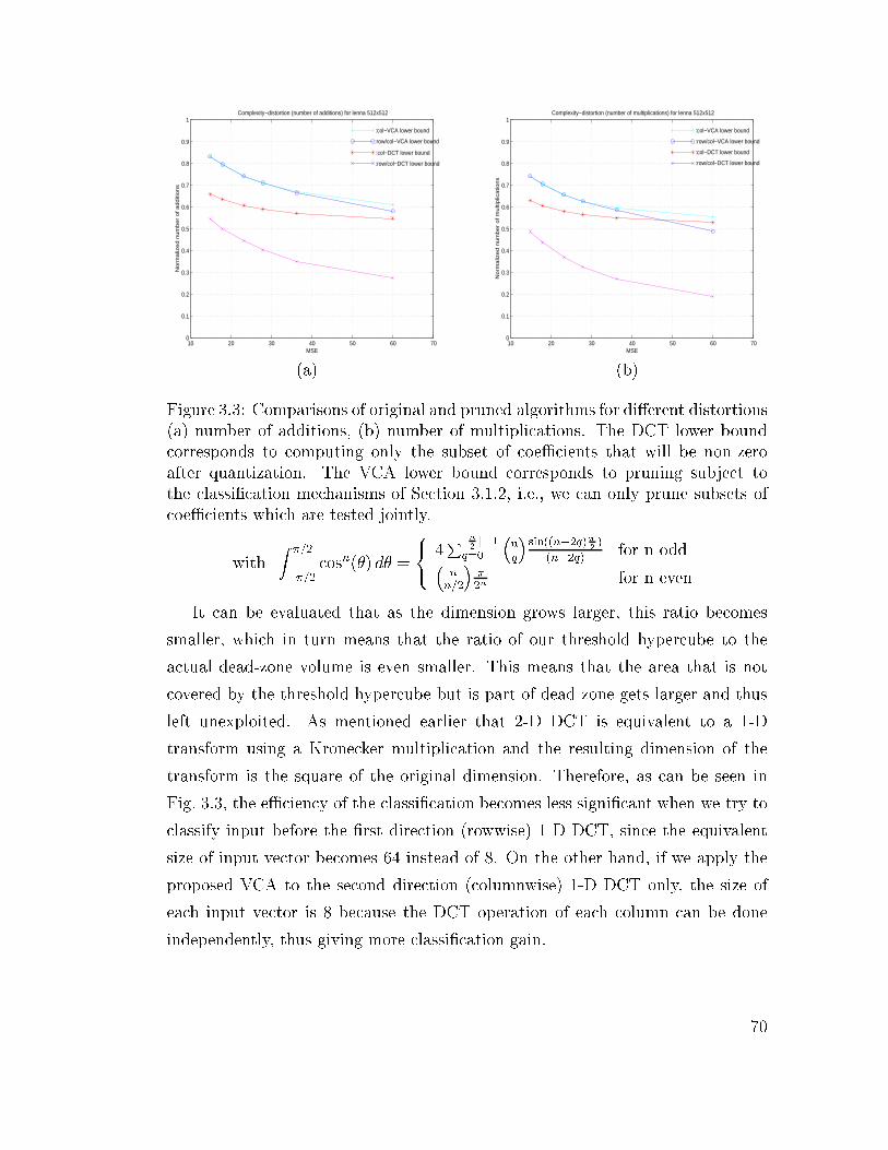
10 20 30 40 50 60 700

0.1

0.2

0.3

0.4

0.5

0.6

0.7

0.8

0.9

1Complexity−distortion (number of additions) for lenna 512x512

MSE

No

rma

lize

d n

um

be

r o

f a

dd

itio

ns

:col−VCA lower bound

:row/col−VCA lower bound

:col−DCT lower bound

:row/col−DCT lower bound

(a)

10 20 30 40 50 60 700

0.1

0.2

0.3

0.4

0.5

0.6

0.7

0.8

0.9

1Complexity−distortion (number of multiplications) for lenna 512x512

MSE

No

rma

lize

d n

um

be

r o

f m

ulti

plic

atio

ns

:col−VCA lower bound

:row/col−VCA lower bound

:col−DCT lower bound

:row/col−DCT lower bound

(b)

Figure 3.3: Comparisons of original and pruned algorithms for di�erent distortions

(a) number of additions, (b) number of multiplications. The DCT lower bound

corresponds to computing only the subset of coeÆcients that will be non-zero

after quantization. The VCA lower bound corresponds to pruning subject to

the classi�cation mechanisms of Section 3.1.2, i.e., we can only prune subsets of

coeÆcients which are tested jointly.

withZ �=2

��=2cosn(�) d� =

8<:

4Pbn

2c�1

q=0

�n

q

�sin((n�2q)�

2)

(n�2q)for n odd�

n

n=2

��2n

for n even

It can be evaluated that as the dimension grows larger, this ratio becomes

smaller, which in turn means that the ratio of our threshold hypercube to the

actual dead-zone volume is even smaller. This means that the area that is not

covered by the threshold hypercube but is part of dead-zone gets larger and thus

left unexploited. As mentioned earlier that 2-D DCT is equivalent to a 1-D

transform using a Kronecker multiplication and the resulting dimension of the

transform is the square of the original dimension. Therefore, as can be seen in

Fig. 3.3, the eÆciency of the classi�cation becomes less signi�cant when we try to

classify input before the �rst direction (rowwise) 1-D DCT, since the equivalent

size of input vector becomes 64 instead of 8. On the other hand, if we apply the

proposed VCA to the second direction (columnwise) 1-D DCT only, the size of

each input vector is 8 because the DCT operation of each column can be done

independently, thus giving more classi�cation gain.

70

The result of the classi�cation is shown in terms of number of operations as

normalized by the fast algorithm in Figure 1.3, which is used for separable row-

column 1-D DCT. We encode the \lenna" image of size 512x512 using di�erent

quantization parameters to obtain the complexity at di�erent qualities for the

decoded images. The DCT computation is exact and the only distortion is that

introduced by quantization. The results of pruning for each quantization level

are shown in Figure 3.3 (a), (b). In these �gures, the classi�cation costs are not

included in order to see the eÆciency of the pre-transform deadzone test compared

to the ideal case where all input points inside the deadzone are detected. Thus

the results indicate the minimal achieveable complexities or the lower bounds. In

Figs. 3.3, we see that the lower bound on complexity reduction using our proposed

VCA is close to the ideal case when applied to the column 1-D DCT only.

3.1.2 Optimal Classi�cation

When the complexity of the tests is taken into account the total complexity can

be higher than that of the original �xed complexity algorithm, as seen in Fig-

ure 3.4. As in Chapter 2, we optimize the classi�cation such that only tests that

provide reductions in average complexity are kept (i.e., the savings achieved when

operations are skipped outweigh the overhead of testing for all inputs). This

optimization is based on training on a set of images and is performed through

exhaustive search (since the number of tests involved is small.)

We use \baboon", \boat", \creek" and \lake" as training data to design the

VCA at each quantization parameter for \lenna" image. The result of both esti-

mated complexity and CPU clock1 savings are shown in Figure 3.4. We use the

same set of weights for operations as in Table 2.1. It can be seen that when the

quantization parameter is small, i.e., in the low MSE region, the complexity is the

same as that of the original �xed complexity algorithm. This means that there

is no test in the algorithm because in the optimization process it is determined

that the tests would not result in any savings. On the other hand, in the high

MSE region, given that there will be more zero outputs, there is something to be

1The implementation is run on a Sun Ultra-1 running Solaris 2.5.

71

10 20 30 40 50 60 70 800.7

0.75

0.8

0.85

0.9

0.95

1

1.05

1.1Complexity−Distortion from implementation

Nor

mal

ized

com

plex

ity (

clk.

/clk

.)

MSE

:Unoptimized VCA

:Optimized VCA

:Simulated Optimized VCA

:Reduced 4x4

:SB−DCT LL

:Approx−Q

Figure 3.4: Complexity(clock cycle)-distortion comparison with \lenna" JPEG

encoding.

gained from the VCA approach as will be seen later in this chapter.

From our results we can see that the gains are modest due in part to the over-

head involved in testing. However a major reason for the lack of more signi�cant

gains is the fact that we are still computing an exact DCT, when in fact at high

MSEs an approximate DCT would be acceptable given that data is going to be

coarsely quantized.

3.2 Approximate DCT

The DCT can be approximated using a subband decomposition as in [48] and

[47]. This approach exploits the fact that, with appropriate post-processing, the

DCT coeÆcients can be obtained after the subband decomposition, and in typical

natural images one can disregard high frequency subband components without

greatly a�ecting the accuracy of the calculated DCT. Therefore, the DCT coef-

�cients can be approximated from post-processing only low frequency subband

coeÆcients. Because a simple subband decomposition can be used (Haar �lters

for example) the overhead for pre-processing is small. A subband decomposition

72

hence can be viewed as a pre-processing that reduces the interdependencies among

the inputs and gives some clues about what information can be disregarded.

Instead of approximating the whole DCT block with a subset of DCT coeÆ-

cients, another approach is to estimate all the coeÆcients but with less accuracy.

In this section, we �rst give a review of the statistical sum of absolute value test-

ing (SSAVT) [64], and analyze the distortion contributed by the approximation.

Also, our proposed approximate algorithm is described, and its error analysis is

discussed.

3.2.1 SSAVT Review

We �rst review the SSAVT [64] algorithm. From the Laplacian model for residue

pixels presented in Section 1.6, we have that the variance of each pixel is (see

(1.5))

�2X(u;v) = �2�2

N(u; v)

where �2N(u; v) is a function of the correlation coeÆcient of spatial domain pixels.

We can �nd the variance of each DCT coeÆcient from the scaled version of the

spatial-domain variance. In [64], the residue pixels are modeled in spatial domain

to be Laplacian distributed with zero mean as in (1.3). This assumption is also

applicable to some extent to pixels in INTRA coded frames. Thus, in this work

we apply the Laplacian model to INTRA coding. Since the fundamental idea of

the SSAVT is to allow looser thresholding by introducing a probabilistic criterion

(as opposed to the deterministic criterion in [61]), a model mismatch for I-frames

would only result in a small deviation in the probabilistic criterion from the ac-

tual one. From this Laplacian assumption, we can estimate �2 from the Sum of

Absolute Value (SAV) as

� �p2 � SAV=N2 (3.4)

where N2 is the number of pixels in an NxN block. In the case of a P-frame, the

SAV can be obtained as a by-product of the motion estimation, since the Sum of

Absolute Di�erence (SAD) is computed and compared in order to �nd the best

motion vector. However, it is worth mentioning that the SAD corresponding to a

macroblock can only be used to obtain a value of � that will be the same for all

73

four 8x8 blocks. In an advanced prediction mode (OBMC), the SAD of each block

is computed and therefore we can have di�erent � for each block. Alternatively,

it would be possible to explicitly compute the SAD for each of the subblocks so

as to have a di�erent � for each.

The key to reducing the complexity comes from the fact that given the model

we can always �nd the range of values that the DCT coeÆcient will take with some

probability. For example, the probability that a value will fall within (�3�; 3�) isabout 99%, and as a result, we can skip the computation of a certain coeÆcient

if the value is 99% sure to be quantized to zero. The testing would then consist

of checking if

3�X(u;v) < 2QP +DZ; (3.5)

where QP and DZ are the quantization parameter and the additional deadzone

factor, respectively. That is, the 99% probability interval is completely embedded

in the deadzone.

3�N(u; v)� < (2QP +DZ)

SAV < (2QP +DZ) �N2=(3p2�N(u; v)) (3.6)

Equation (3.6) is from (3.4). Therefore, the test is equivalent to a threshold

testing of the SAV . The con�dence level can also be changed depending on the

complexity reduction versus accuracy tradeo�. Furthermore, from (1.6) it can

be seen that the variances are decreasing from the DC to higher frequency AC

coeÆcients. This implies that if a lower frequency DCT is determined to be zero,

so are all higher frequency DCTs. As a result, the classi�cation can be performed

by testing the SAV with a set of thresholds which corresponds to classifying the

output 8x8 DCT block to i) all-zero, ii) DC-only, iii) low-4x4, and iv) all-64. For

each of the test, �8(0; 0);�8(1; 0) and �8(4; 0) are used in (3.6), respectively.

The result of this classi�cation is very promising. Only a slightly degradation

in PSNR is observed because the distortion caused by not computing high fre-

quency components is compensated by the corresponding bit savings. We now

provide an analysis of the distortion introduced by the SSAVT that was not pro-

vided by the original authors [64] and which will help us evaluate the degradation

74

introduced by the SSAVT and compare it with that of our proposed approximate

algorithms.

3.2.2 Error Analysis of SSAVT

For each outcome of the SAV test, a corresponding reduced output DCT is ap-

plied. We can then consider the reduced output DCT as an approximation of the

exact DCT. For example, the equivalent transform matrix of the low-4x4 DCT is24 I4 0

0 0

35D8 where I4 is the 4x4 identity matrix. In words, it is D8 with all the

lower 4 rows, and rightmost 4 columns, set to zero. Therefore, di�erent approxi-

mate DCTs are used for di�erent values of �2. Let fTh0; Th1; :::; ThGg be a set ofthresholds de�ned as functions of QP for classifying an input into G classes (e.g.,

for the SSAVT, G is 4) where Th0 is 0 and ThG = 1. The i-th reduced output

DCT is applied if Thi�1 � � < Thi. where � is the approximation of � computed

from the SAV and

Thi =2QP +DZ

3 max(u;v)2Bi

�N(u; v)(3.7)

where Bi is a set of output coeÆcients computed. Therefore, the block distortion

of class i input can be expressed as

Dssavt(Bi) =X

(u;v)2BiD(u; v) +

X(u;v)=2Bi

�2�2N(u; v) (3.8)

where D(u; v) is obtained from (1.10).

The �rst term is the sum of the distortion of coeÆcients that are computed,

and the second term corresponds to the coeÆcients that are computed and thus

are not coded. Figure 3.8 shows the normalized increase in distortion using the

SSAVT at various �2 and QP (ratio between the second term and the �rst term

of (3.8)). This result is based on the assumption that the variance of the signal

can be perfectly estimated from the SAV.

It can be seen that the increases in distortion have a seesaw shape as a function

of the pixel variance. This can be explained as follows. For a given QP, there is a

set of thresholds that speci�es which reduced DCT will be used within a certain

75

100

101

102

103

0

0.02

0.04

0.06

0.08

0.1

0.12Normalized Additional Distortion for SSAVT

pixel variance σ2

QP=10

QP=20

QP=30

Figure 3.5: Additional distortion (normalized by the original distortion) when

using SSAVT at various levels of the pixel variance �2.

interval. At the beginning of each new interval, an algorithmwhich computes more

coeÆcients is selected thus pushing the distortion down, and as the �2 grows, the

extra distortion starts to become larger again. For the SSAVT algorithm, there

are 3 thresholds. After the third threshold has been exceeded (at the right end

of each curves in Fig. 3.8), there is no additional distortion since all 64 DCTs are

always computed. As an extension to [64], we perform SSAVT for all possible

reduced output DCTs, i.e., we also consider low-2x2 output class as well. In other

words, c(A�i ) will have the form shown in (2.7).

The reduction in computation and the increase in distortion from computing

only a subset of DCT coeÆcients has a bene�t in that the overall rate required

to code the DCT coeÆcients is reduced. Therefore, the rate and complexity of a

class g input can be written as

Rssavt(Bi) =X

(u;v)2BiR(u; v) (3.9)

Tssavt(Bi) = c(A�i ) + i � c(Av); (3.10)

when Thi � � < Thi + 1.a c(Av) is the cost for SAV threshold testing.

In order to �nd �Dssavt, �Rssavt, and �Tssavt, the average values of distortion, rate

and complexity, the probability of the outcomes of the SAV test has to be taken

76

into account. For a given model of the source, the variance �2 cannot be perfectly

estimated by the SAV. The mean absolute sum m = SAV=N2 can be viewed as

a random variable representing the time average of the source. It can be derived

from the model of the source (�rst order Markov source) that the mean of m is

Efmg = �=p2

and the variance is

�2m = Ef(m� Efmg)2g = �2(

1

N2+2((N2 � 1)��N2�2 � �N

2+1)

N4(1� �)2);

where, again, � is the correlation coeÆcient of the source.

Let us denote the approximation of �2 based on m and �2 = 2m2. This �2 is

tested with a set of thresholds fTh0; Th1; :::; ThGg where G = log2N + 1 for all

possible reduced output DCT. The probability of each outcome of the threshold

test can be written as

Pi =Z Thi+1

Thi

f2m2(x)dx

=Z pThi+1=2

pThi=2

fm(x)dx (3.11)

where fm(x) is the p.d.f. of m. From [88] (see also Chapter 2), the di�erence

between the partial mean of absolute pixel di�erence (PMAD) and the actual

mean of absolute pixel di�erence (MAD) is modeled as a Laplacian distribution.

Therefore, in this thesis, we assume thatm has a truncated Laplacian distribution

with mean and variance as above, i.e.,

fm(x) =

8<:

�s2Le��jx�Efmgj for x > 0

0 otherwise

where L =R10 �me

��jx�Efmgj is a constantnormalization factor that ensures that

a valid p.d.f. is obtained and �m = �m=p2. Thus, the complexity, rate and

77

distortion can be expressed in a similar fashion to (2.9) as

�TSSAV T =log2 N+1X

i=1

Pi � Tdyadic(Bi) (3.12)

�RSSAV T =log2 N+1X

i=1

Pi �Rdyadic(Bi) (3.13)

�DSSAV T =log2 N+1X

i=1

Pi �Ddyadic(Bi) (3.14)

Note that all the above quantities are functions of QP, �2 and N . The R-C-D

characteristic of the SSAVT is shown in Figure 3.6.

050

100150

200

0

5

10

15

x 106

0

0.5

1

1.5

2

2.5

distortion (mse)

Rate−Complexity−Distortion of SSAVT

complexity

σ2=700

σ2=500

σ2=300

σ2=100

rate

(bi

t/pix

el)

Figure 3.6: Rate-complexity-distortion functions of SSAVT. The R-C-D results of

SSAVT and ideal dyadic test are very close and hence cannot be visually distin-

guished in the �gure.

Figure 3.7 shows the complexity comparison between the SSAVT and the 2-D

dyadic classi�cation. Since the DCT and IDCT operations are transpositions of

each other, the 2-D dyadic classi�cation for IDCT in Chapter 2 can be considered

as the ideal case for SSAVT where all instances of reduced output DCT are 100%

correctly detected. The addition and multiplication results follow a similar trend

as the total complexity curve, and are thus omitted here. The R-D function of the

SSAVT is already shown in Figure 1.8. It can be seen that the R-D performance

78

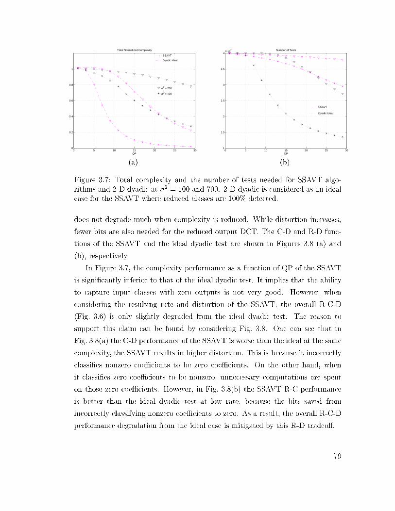
0 5 10 15 20 25 300

0.2

0.4

0.6

0.8

1

QP

Total Normalized Complexity

SSAVT

Dyadic ideal

:σ2 = 700

:σ2 = 100

(a)

0 5 10 15 20 25 301

1.5

2

2.5

3

3.5

4x 10

4

SSAVT

Dyadic Ideal

QP

Number of Tests

(b)

Figure 3.7: Total complexity and the number of tests needed for SSAVT algo-

rithms and 2-D dyadic at �2 = 100 and 700. 2-D dyadic is considered as an ideal

case for the SSAVT where reduced classes are 100% detected.

does not degrade much when complexity is reduced. While distortion increases,

fewer bits are also needed for the reduced output DCT. The C-D and R-D func-

tions of the SSAVT and the ideal dyadic test are shown in Figures 3.8 (a) and

(b), respectively.

In Figure 3.7, the complexity performance as a function of QP of the SSAVT

is signi�cantly inferior to that of the ideal dyadic test. It implies that the ability

to capture input classes with zero outputs is not very good. However, when

considering the resulting rate and distortion of the SSAVT, the overall R-C-D

(Fig. 3.6) is only slightly degraded from the ideal dyadic test. The reason to

support this claim can be found by considering Fig. 3.8. One can see that in

Fig. 3.8(a) the C-D performance of the SSAVT is worse than the ideal at the same

complexity, the SSAVT results in higher distortion. This is because it incorrectly

classi�es nonzero coeÆcients to be zero coeÆcients. On the other hand, when

it classi�es zero coeÆcients to be nonzero, unnecessary computations are spent

on those zero coeÆcients. However, in Fig. 3.8(b) the SSAVT R-C performance

is better than the ideal dyadic test at low rate, because the bits saved from

incorrectly classifying nonzero coeÆcients to zero. As a result, the overall R-C-D

performance degradation from the ideal case is mitigated by this R-D tradeo�.

79

0 5 10 15

x 106

0

10

20

30

40

50

60

70

80Complexity−Distortion for σ2 = 100


Dis

tort

ion

(mse

):SSAVT

:Dyadic Ideal

:DCT 16x16

:DCT 8x8

:DCT 4x4

(a)

0 5 10 15

x 106

0

0.2

0.4

0.6

0.8

1

1.2

1.4Rate−Complexity for σ2=100


Rat

e (b

it/pi

xel)

:SSAVT

:Dyadic Ideal

:DCT 16x16

:DCT 8x8

:DCT 4x4

(b)

Figure 3.8: (a) Complexity-distortion and (b) Rate-complexity curves for di�erent

algorithms, i.e., SSAVT ('solid') and 2-D dyadic ('dashed'), for DCT size 16x16

('x'), 8x8 ('o') and 4x4 ('*') at �2 = 100. 2-D dyadic is considered as an ideal

case for the SSAVT where reduced classes are 100% detected.

b

SSAVT is an example of the superior performance of approximation approaches

as compared to exact VCA approaches. However, in the next section, as an al-

ternative to the SSAVT in which only a subset of the outputs is computed, we

propose another class of approximate algorithms in which all the outputs are

computed at an accuracy lower than the minimum requirement of the standard

DCT.

3.2.3 APPROX-Q DCT

Here we introduce an approximate algorithm (see also [66]) where in the DCT

coeÆcient computation we replace the multiplications with additions and binary

shifts in a manner that is quantization dependent. For large QP, a coarse approxi-

mate DCT is used because even if the error in coeÆcient computation is large, the

large quantization step means that their quantized representation will introduce

even more error. Similarly, �ner approximate DCT is used when QP is small. Our

proposed approximate DCT is shown in �gure 3.9. This �gure is derived from the

fast DCT in 1.3 by simplifying the operations. The matrix po ranges from the

80

x0

x1

x2

x3

x4

x5

x6

x7

POi

W0X0

W4X4

W2X2

W6X6

W5X5

W1X1

W7X7

W3X3

Figure 3.9: The approximate DCT algorithm.

identity matrix, po1 =

24 q1 0

0 I

35, to more complex matrix po2,po3,po4,and po5

shown below.

po2 =

26666666664

q1 �0t �0t �0t �0t

�0 1 0 1=8 �1=8�0 �1=8 1 1=8 0

�0 0 �1=8 1 1=8

�0 1=8 1=8 0 1

37777777775

po3 =

26666666664

q2 �0t �0t �0t �0t

�0 1 1=8 1=8 �1=8�0 �1=8 1 1=8 �1=8�0 �1=8 �1=8 1 1=8

�0 1=8 1=8 �1=8 1

37777777775

po4 =

26666666664

q3 �0t �0t �0t �0t

�0 1 1=8 1=8 �1=4�0 �1=8 1 1=4 �1=8�0 �1=8 �1=4 1 1=8

�0 1=4 1=8 �1=8 1

37777777775

81

Table 3.1: Number of operations required for proposed approximate algorithms

where Alg. No. i corresponds to using the transform matrix Poi.

Alg. No. Additions Multiplication Binary Shifts

1 24 0 2

2 33 0 7

3 38 0 8

4 42 0 12

Vetterli's [29] 29 13 0

po5 =

26666666664

q3 �0t �0t �0t �0t

�0 1 1=8 1=8 �3=16�0 �1=8 1 3=16 �1=8�0 �1=8 �3=16 1 1=8

�0 3=16 1=8 �1=8 1

37777777775

where

q1 =

24 1 �1=21=2 1

35

q2 =

24 1 �3=81=2 1

35

q3 =

24 1 �3=83=8 1

35

�0 = [ 0 0 ]

The number of operations required for these approximate DCTs are shown in

Table 3.1.

Let an approximate DCT matrix using one of the above approximations be de-

noted by (Dapprox). After these approximations, if one wants to obtain the exact

DCT coeÆcient values, the post-transform matrix would be D8 �Dapprox�1. This

post-transform matrix gets closer to the identity matrix (up to scaling factors) as

the approximation gets more accurate. The scaling factors needed at the output

can be found to be diag(D8 �Dapprox�1), and can be absorbed in quantization,

82

i.e., in our approximate DCT, the post-transform is approximated by setting o�-

diagonal elements to zero leaving only the diagonal elements as scaling factors.

Since this algorithm is lossy, the approximation introduces more distortion to

the reconstructed images. The rate-distortion curves of these approximate DCTs

using JPEG coding are shown in Figure 3.10.

0 0.5 1 1.526

28

30

32

34

36

38Rate−Distortion of different DCT alg. for "lenna"

SN

R

Bit per pixel

:SB−DCT LL

:Exact DCT:Approx−Q DCT

:Approx#5:Approx#4:Approx#3

:Approx#2

:Approx#1:Reduced 4x4

Figure 3.10: Rate-Distortion curve of 512x512 lenna image JPEG coding using

various DCT algorithms. Note that at high bit rate coarser approximate algo-

rithm performances deviate from the exact DCT performance dramatically. The

quantization dependent approximation can maintain the degradation level over

wider range of bit rate.

In this experiment, we encode the \lenna" image with JPEG compression

using the example quantization matrix [1]. It can be seen that, as expected, in

the high distortion region the increase in distortion introduced by the approximate

DCTs does not a�ect performance because it is less than the distortion due to

quantization. Therefore, we develop an algorithmwhich is quantization parameter

dependent (shown as a solid line, Approx-Q, in Figure 3.10) in which the selection

of the approximate algorithm is made at the beginning of the encoding process

depending on the quantization parameter. It uses a coarser DCT approximation

algorithm for low quality coding and �ner DCT approximation for high quality

coding for small degradation. The degradation of the decoded image introduced

by the approximate DCT is 0.12 dB at 0.18 bpp, 0.15 dB at 0.91 bpp and 0.64 dB

83

at 3.17 bpp. From Figure 3.10, it is obvious that even with the Approx#2, the R-

D curve is better than other reduced complexity approximate algorithms such as

pruned DCT (computing only low frequency 4x4 DCT) and subband DCT (using

low-low subband [48]). This is because we do not lose high frequency information

which is present at high rates.

3.2.4 APPROX-Q Error Analysis

We now analyze the additional distortion introduced by the approximation of the

DCT and, based on that, we show how to automatically select which (coarser

or �ner) approximate DCT should be used for a given QP and �2 . Our goal

is selecting the algorithm to ensure that the resulting overall distortion does not

exceed a certain level.

Let us denote the transform matrix of the i-th approximate DCT by Di, the

input spatial domain block x, and the DCT computed by this reduced matrix by

Xi. Therefore, the di�erence between the exact and approximate computation

can be written as

e = X� Xi

= DxDt � DixDti

= (D� Di)x(D� Di)t

= EixEti (3.15)

where Ei = D� Di is the approximation error matrix. With a similar analysis to

that in Section 1.6, the variance of the error in DCT domain can be derived as

�2e(u; v) = �2[EiRE

ti ](u;u)[EiRE

ti ](v;v) = �2�2

i (u; v); (3.16)

where R is the correlation matrix of the input vector and �2i (u; v) is a scaling

constant that is a function of the approximation matrix. In general �2i (u; v) should

be much smaller than �2N(u; v), since their ratio is the relative additional distortion

introduced by the approximation. The total block approximate error can be

84

written as De(q),

De(q) = �2X(u;v)

�2q(u; v) (3.17)

We can model this approximation error as an additive white Gaussian noise

(AWGN) that is to be added to another AWGN error due to quantization, i.e.,

from the approximate quantized DCT, ~X can be written as

~X = X+ nq + na

where nq is a Gaussian r.v. modeling the error due to quantization and na repre-

sents another Gaussian r.v. representing the approximation error. It is reasonable

to assume that nq and na are independent. Therefore, the distortion can be ex-

pressed in terms of the summation of the original distortion and the distortion

from approximation.

DAPPROX(QP; �2; N) =

X(u;v)

D(u; v) +De(q) (3.18)

0 100 200 300 400 500 600 70010

−8

10−7

10−6

10−5

10−4

10−3

10−2

10−1

Normalized Additional Distortion for Approx−DCT

pixel variance σ2

solid: QP=2

dashed:QP=10dotted:QP=30

#1

#3

#2

#4

#5

Figure 3.11: Additional distortion (normalized by original distortion) using ap-

proximate DCT algorithms #1 ('�'), #2 ('5'), #3 ('o'), #4 (''), and #5 ('�')at various pixel variance �2.

Figure 3.11 shows the approximation error results of the 5 approximate DCT

algorithms normalized by the distortion due to quantization. It can be seen that

85

not only the approximation error depends on the QP, it also increases as the pixel

variance �2 grows, i.e., for a �xed pixel variance the additional error ratio increases

as quantization stepsize decreases. Furthermore, for a �xed QP, the additional

error ratio increases with pixel variance. However, for a given approximate al-

gorithm, QP still plays a bigger role in the resulting error. Therefore, we can

systematically select which approximate algorithm to be used for a given QP and

�2, so as to ensure that the approximation error is below a certain limit, i.e.,

the q-th algorithm is selected if De(q) < �X(u;v)

D(QP; �2; N)

where � is the level of desired additional error . For example, when coding a

frame with �xed QP for all blocks, low variance blocks (associated with low activ-

ity) require less accurate DCT approximation whereas high variance blocks must

use �ner approximation in order to maintain the same level of additional error

throughout the entire frame.

3.3 Results and Hybrid Algorithms

In this section we discuss a series of hybrid algorithms which combine the strengths

of each the previously proposed algorithms. Experimental results are shown based

on the baseline H.263 TMN's codec [58] used to encode 249 frames of the \Fore-

man" sequence at di�erent target bit rates. The Visual C++ compiler with op-

timization option is used. The CPU clock cycles spent in both the DCT and

quantization are measured because for the VCA exact DCT, not only the DCT

can be prunned but also the quantization for those zero coeÆcients can be omit-

ted. For Approx-Q, since the approximated coeÆcients have to be scaled, the

extra scaling operation has to be done in the quantization process thus a�ecting

the overall complexity. However, it will be seen later that the speedup from the

DCT part is much more signi�cant than the slowdown in quantization for the

Approx-Q case. As can be seen in Fig. 3.12, the speedup of the Approx-Q is

much higher than the VCA exact algorithm with only 0.01-0.06 dB degradation.

86

0.2 0.3 0.4 0.5 0.6 0.7 0.8 0.9 1 1.1 1.227

27.5

28

28.5

29

29.5

30

30.5

31

31.5DCT + quantization complexity results of "foreman"

PS

NR

Normalized complexity

50 Kbps

40 Kbps

30 Kbps

20 Kbps

ASSAVT−VCA

Approx−VCA

ASSAVT SSAVTApprox−Q VCA

Figure 3.12: The complexity (CPU clock cycle) of the DCT + Quant. normalized

by the original algorithm in TMN at various PSNRs (di�erent target bit rates) of

original DCT ('+'), SSAVT ('o'), Approx-Q ('4'), ASSAVT ('2'), Approx-VCA

('5'), and ASSAVT-VCA ('*').

3.3.1 Approx-SSAVT (ASSAVT)

We �rst combine the SSAVT and the Approx-Q DCT in such a way that the SAV

is �rst tested and the input is thus classi�ed in the same manner as the SSAVT.

Then the reduced DCT is approximated using the approximate algorithm. That

is, we use approximate algorithms also for the reduced dimension DCTs used in

SSAVT. The total block distortion for this combined algorithm, which we call

ASSAVT, can be expressed as

DASSAV T (QP; �2; N) =

X(u;v)2Bi

[D(u; v) + �2�2i (u; v)] +

X(u;v)=2Bi

�2�2N(u; v) (3.19)

The �rst summation on the right side is the distortion plus approximation er-

ror of the computed coeÆcients. The second term is for uncomputed coeÆcients.

Figure 3.13 shows the result of ASSAVT with the target approximation error at

2x10�4 of the original distortion. For simplicity, this experiment assumes that the

variance of the input is perfectly estimated by the SAV. Therefore, the class that

the input belongs to is deterministic. Therefore, the estimated SSAVT distortion

87

is known with certainty. In practice, the estimation of the pixel variance is ran-

dom, thus resulting in a probabilistic estimation of the SSAVT distortion. The

actual deviation from the SSAVT distortion must be averaged over the support

of the estimated pixel variance. In Figure 3.13, it can be seen that the additional

distortion follows the SSAVT seesaw-shaped results except that it can now be

kept under the speci�ed error bound. Thus, when the error from SSAVT becomes

too small, i.e., suÆcient coeÆcients are computed for the given �, then we can

observe the error due to the approximation. Except in those cases, the additional

error due to approximation is negligible. Moreover, these situations occur when

error is small, anyway, and therefore adding the approximate algorithm to SSAVT

is always bene�cial.

100

101

102

103

10−6

10−5

10−4

10−3

10−2

10−1

100

Normalized Additional Distortion by ASSAVT

pixel variance σ2

QP=10

QP=22

:ASSAVT

:SSAVT

Figure 3.13: Additional distortion (normalized by original distortion) using the

ASSAVT with 2x10�4 target deviation from the original distortion ('- -'), SSAVT

('{'), at QP = 10 ('o') and 22 ('*'), respectively.

We apply the ASSAVT to the DCT subroutine of the TMN [58] H.263 codec

with some modi�cations. First, the reduced DCT, i.e., 2x2-DCT and 4x4-DCT,

use Approx#4 and Approx#5, respectively. This follows the result in Fig 3.13 that

as the variance �2 gets larger, the error becomes larger too. This also results in

larger size DCT after SSAVT classi�cation. Therefore, in order to maintain a small

error, �ner approximation algorithm has to be used. For DC-only class, the DC

coeÆcient can be computed precisely using only additions and a binary shift. For

88

the full DCT class, we use the APPROX-Q algorithm presented earlier in which

the selection of the approximate algorithm is quantization parameter dependent.

The quantization can also be done faster using the result of SSAVT classi�cation,

i.e., the high frequency DCT components do not need to be quantized if they are

not computed. Note that the approximate algorithm assignment can be changed

according to the performance degradation requirement. In our experiments, we

simply select a scheme that gives reasonable complexity reduction and degradation

tradeo�s.

The results of the proposed ASSAVT as compared to SSAVT are shown in

Figure 3.12. The CPU clock cycle of both DCT and quantization are measured as

mentioned above. It can be seen that the ASSAVT can obtain 47-55 % complexity

reduction, as compared to 17-33% reduction by the SSAVT, while the coding

performance is degraded only by 0.04-0.14 dB as compared to 0.02-0.08 dB by

SSAVT with respect to the exact algorithm.

3.3.2 Approx-VCA DCT

It is worthwhile pointing out here that since the structure of the approximate DCT

algorithm is similar to the fast algorithm in Figure 1.3 we can apply the classi�-

cation structure and the optimization technique to obtain the optimal VCA as in

Section 3.1 for the Approx-Q DCT algorithm presented in Section 3.2. The algo-

rithm is now data-dependent and will be called Approx-VCA DCT. Experimental

results are also shown in Fig. 3.12. In this experiment, we also take advantage

of the zero information from the VCA in the quantization process as mentioned

earlier, i.e., if the resulting coeÆcients from VCA are zero, no quantization oper-

ation is needed. In practice, one could combine VCA DCT and quantization into

one subroutine, but for simplicity we still separate them and simply introduce a

zero test before quantizing each coeÆcient.

3.3.3 ASSAVT-VCA DCT

Finally, we can combine SSAVT, Approx-Q and VCA exact DCT into one al-

gorithm. Based on the ASSAVT in Section 3.3.1, we modify the approximate

89

algorithm in the case of all-8x8 class to have pre-transform deadzone test capa-

bility as in Approx-VCA. The result is also shown in Fig. 3.12. It can be seen

that the C-D result is improved from the ASSAVT by about 8-10%. However,

when compared to the Approx-VCA algorithm, the ASSAVT-VCA improves just

a very small fraction at low rates and shows almost no improvement at high rate.

This is because the SSAVT classi�cation eÆciency drops at high rates.


We have proposed two techniques for fast VCA DCT computation. The �rst

one computes exact DCT coeÆcients in a VCA manner by checking on the pre-

transform deadzone region. This algorithm is hierarchical in the sense that the

classi�cation can be broken down to smaller group of coeÆcients. However, the

drawback of this algorithm is the eÆciency of the pre-transform deadzone drops

rapidly as the dimension of the transform grow. Thus we apply it only to the

second 1-D DCT. At high rate, this algorithm shows almost no gain. The sec-

ond technique was then considered. Unlike the �rst approach, the resulting DCT

output is not exact. We gave a review of the reduced DCT using SSAVT classi�ca-

tion and analyzed the performance. Then we proposed an approximate algorithm

that computes all the DCT coeÆcients in a block with less accuracy than in the

exact case. The complexity reduction comes from using cheaper arithmetic opera-

tion (no multiplications) with the sacri�ce in slightly poorer coding performance.

Finally, we showed some experimental results and suggested several hybrid algo-

rithms that combine all the above mentioned algorithms.

It can be seen that the result of approximate techniques are much more promis-

ing than the exact algorithms in terms of complexity at the cost of only a slight

degradation in picture quality. Since the DCT cannot be computed exactly using

any �xed precision computer, the error is already introduced. Also, the quantiza-

tion e�ect masks out the computational error in the case of low rate. This results

in a slight decrease in the overall performance. Another conclusion is that using

the statistical model, such as SSAVT, allows more classi�cation gain with a small

coding performance degradation.

90

Chapter 4

Motion Estimation: Probabilistic

Fast Matching

In this chapter, we propose a matching algorithm for motion estimation that uses

probabilistic stopping criterion based on the partial distance search [79]. It can

be categorized as a computationally scalable Fast Matching (FM) algorithm. The

basic idea is to stop the computation of the matching metric when the partial

metric indicates that the total metric is likely to exceed that of the best candidate

so far. This allows us to save in computation when \bad" candidate vectors are

being tested, since these can be discarded before all pixels in the macroblock have

been used to compute the metric. To achieve this goal we formalize a hypothesis

testing framework where the decision to stop the metric computation is done

based on probabilistic models of the distribution of the actual metric based on

the calculated partial metric. We select a given probability of error (i.e., missing

a \good" vector) based on these models and by varying this probability we can

achieve a computationally scalable calculation. From the nature of the test, we will

refer to the original partial distance search as determinictic testing fast matching

(DTFM) as opposed to the hypothesis testing fast matching (HTFM) ([88],[101])

for the proposed algorithm.

This chapter is organized as follows. In Section 4.1, the original partial dis-

tance algorithm is reformalized and a new macroblock partitioning is introduced.

In Section 4.2, we provide a formal description of the hypothesis testing framework

91

that forms the basis of our algorithm. We model our variables of interest and as-

sume that their second order statistics are known. With a given error probability

or probability of false alarm, we design the hypothesis testing such that the error

probability meets the requirements. We also show simulation results on some test

sequences where we assume all necessary statistics of a particular sequence are

known to the encoder. In Section 4.3, since each sequence has di�erent character-

istics which are unknown to the encoder before the encoding process takes place,

we discuss how to obtain the statistics adaptively during the encoding. As an

extension to [86], we propose an alternative computationally scalable Fast Search

(FS) in Section 4.4.1 which can be combined with our HTFM. Finally, in Section

4.4, we show the result of our proposed HTFM with adaptive parameter estima-

tion as compared to DTFM using ES, 2-D Log search [68] and ST1 search [4].

Finally, concluding remarks are given in Section 4.6.

4.1 Partial Distance Fast Matching

In this work, we use SAD as the matching criterion1 (refer to Table 1.3 for nec-

essary notations). In all our experiments SAD calculations are based on at most

128 pixels out of the 256 pixels of a macroblock. As in [67], this subset �q � B

is obtained by subsampling using a quincunx grid (see Fig. 4.1.) As shown by

Fig. 4.2, this particular subsampling tends to provide suÆcient accuracy for the

SAD calculation (see [67, 4]), i.e., the overall MSE does not increase signi�cantly

if we use �q instead of B.

Our work is based on splitting each set �q into b subsets of pixels, yi, for

i 2 f1; 2; :::; bg, such thatSbi=1 yi = �q and yi \ yj = � for i 6= j (see for example

Fig. 4.1). Let us de�ne xi =Sij=1 yj. During the SAD calculation of ~mvj, we

compare the partial calculation of the SAD, SAD( ~mvj; xi) with the best SAD

obtained out of all previously tested candidates, SADbsf( j�1; �q). If the partial

SAD is greater than SADbsf , we can terminate the computation and continue to

1Note, however, that our approach could be easy generalized to other additive distancemetrics such as MSE (see for example our work in applying this approach to searching of aVector Quantizer codebook in [101]).

92

the next vector. Otherwise, we compute SAD( ~mvj; xi+1) for the next stage and

perform the test again. If no early termination occurs, the process repeats until

the �nal stage, b, is reached.

There are many possible ways to partition �q into subsets yi. In this work, we

propose two methods, which both have jyij = 8, 8i, and thus result in 16 stages

of testing: these are the uniform partition (UNI)2 and the row-by-row partition

(ROW) shown in Fig.4.1(a) and 4.1(b), respectively. In Fig.4.1(a), the partition

is designed such that the correlation between SAD( ~mv; �q) and SAD( ~mv; xi) is

maximum, given that the pixels are uniformly spaced. This results in fewer pixel

comparisons on the average, since early termination is more likely. However,

for a hardware implementation, UNI may not be desirable as it results in more

irregular memory access patterns. Conversely, ROW (see Fig.4.1 (b)) provides a

more regular memory access that could simplify the implementation, although we

can expect ROW to be worse than UNI in terms of producing a reliable estimate

of the total SAD.

To simplify the notation, when there is no ambiguity we omit to write the

terms ~mvj, j�1 and B. Also we use PSADi to represent the partial SAD at

stage i, i.e., SAD( ~mv; xi) for i = 0; :::; b � 1. Note that the partial SAD can be

computed recursively as

PSADi+1 = PSADi + SAD( ~mv; yi) (4.1)

where PSAD0 = 0 and PSADb = SAD.

It is clear from (4.1) that PSADi � SAD, for 8i. Therefore, if PSADi is

greater than the SADbsf , there is no need to complete the SAD computation and

we can move on to evaluate the next vector. Otherwise, we compute PSADi+1

and perform the test again. As a result the MV � obtained by the partial distance

method is obviously the same as that obtained by computing directly the full

metric. Thus we call this technique a deterministic testing fast matching (DTFM),

2During the reviewing process of our paper [89], we became aware of the work by Chengand Sun [102], which independently proposed using a uniform partition (dithering pattern pixeldecimation). It is important to note, however, that neither this or other FM works use a variablenumber of pixels for matching.

93

1 5 1 5 1 5 1 5

9 13 9 13 9 13 9 13

7 3 7 3 7 3 7 3

15 11 15 11 15 11 15 11

2 6 2 6 2 6 2 6

10 14 10 14 10 14 10 14

8 4 8 4 8 4 8 4

16 12 16 12 16 12 16 12

1 5 1 5 1 5 1 5

9 13 9 13 9 13 9 13

7 3 7 3 7 3 7 3

15 11 15 11 15 11 15 11

2 6 2 6 2 6 2 6

10 14 10 14 10 14 10 14

8 4 8 4 8 4 8 4

16 12 16 12 16 12 16 12

(a)

1 1 1 1 1 1 1 1

2 2 2 2 2 2 2 2

3 3 3 3 3 3 3 3

4 4 4 4 4 4 4 4

5 5 5 5 5 5 5 5

6 6 6 6 6 6 6 6

7 7 7 7 7 7 7 7

8 8 8 8 8 8 8 8

9 9 9 9 9 9 9 9

10 10 10 10 10 10 10 10

11 11 11 11 11 11 11 11

12 12 12 12 12 12 12 12

13 13 13 13 13 13 13 13

14 14 14 14 14 14 14 14

15 15 15 15 15 15 15 15

16 16 16 16 16 16 16 16

(b)

Figure 4.1: Subset partitionings for 128 pixels subsampled using a quincunx grid

into 16 subsets for partial SAD computation. Only highlighted pixels are used

to compute SAD. Two types of subsets are used (a) uniform subsampling (UNI)

and (b) row-by-row subsampling (ROW). Partial distance tests at the i-th stage

are performed after the metric has been computed on the pixels labeled with i

(corresponding to yi).

as it deterministically provides the optimal solution. Note that in this work we

call \optimal" the motion vector that is obtained with SAD computed from �q

(i.e., 128 pixels). Therefore a solution based on xi � �q will tend to be \sub-

optimal" since we cannot guarantee that it will produce the same motion vector

selection obtained using �q. The DTFM approach can be summarized as follows

Algorithm 2 (DTFM)

Step 1: At the beginning of motion search for a particular block, compute the

SAD of the �rst candidate MV, assign it to SADbsf and set MVbsf accordingly.

Step 2: Every time a new ~mv is considered, as dictated by the FS strategy, set

SAD to zero. Set i = 0. If there is no next unevaluated vector, MV � =MVbsf .

Step 3: Compute PSADi

Step 4: If i < b, go to step 5, else let SAD = PSADb and go to step 6.

Step 5: If PSADi � SADbsf , we eliminate the current candidate and go to

step 2. Otherwise, let i = i+ 1 and repeat step 3.

Step 6: If SAD < SADbsf , SADbsf = SAD and MVbsf = ~mv. Go to step 2.

94

0 0.1 0.2 0.3 0.4 0.5 0.6 0.7 0.8 0.9 1−0.45

−0.4

−0.35

−0.3

−0.25

−0.2

−0.15

−0.1

−0.05

0Complexity−distortion for full search

normalized clock cycle

PS

NR

deg

rada

tion

(a)

0.2 0.3 0.4 0.5 0.6 0.7 0.8 0.9 1−0.4

−0.35

−0.3

−0.25

−0.2

−0.15

−0.1

−0.05

0Complexity−distortion for ST1 search


PS

NR

deg

rada

tion

(b)

Figure 4.2: Complexity-Distortion of reduced set SAD computation with ROW

DTFM ('dotted') and without DTFM ('solid') using (a) ES and (b) ST1 search,

averaged over 5 test sequences. Points in each curve from right to left correspond

to j�j = 256, 128, 64 and 32, respectively. Note that there is a minimal di�erence

between computing the SAD based on 256 and 128 pixels. For this reason in all

the remaining experiments in this work we use at most 128 pixels for the SAD

computation.

The partial distance technique we have just described is well-known and is

implemented in many actual software implementations, where ROW subsampling

is typically used (e.g. [58],[103]). The complexity savings of this technique come

from the possibility of early termination in Step 5. The amount of complexity

reduction varies depending on the nature of the sequence. Also, since we can use

DTFM with any FS algorithm, the eÆciency of the FS algorithm will a�ect the

savings stemming from DTFM. For example, for eÆcient FS algorithms the tested

MVs are likely to have small SAD and their SAD values will tend to be fairly

similar. Therefore there is less chance to terminate the matching computation

at an early stage, and the bene�ts of DTFM will be reduced. In general, the

complexity reduction contributed by DTFM can be signi�cant, e.g., about 3-5

times speedup in the ES case. In Fig.4.2, complexity-distortion (C-D) results with

and without DTFM are compared. The C-D curves are obtained by changing the

set �. One can observe that the relative gain in using DTFM is lower when a fast

search algorithm is used (see also Table 1.1).

95

4.2 Hypothesis Testing Framework

In this section, we propose an algorithm, hypothesis testing fast matching (HTFM),

that enables additional complexity savings as compared to DTFM by allowing an

early termination of the SAD calculation based on the likelihood that the SAD

will be greater than SADbsf , given the current PSADi. This complexity reduc-

tion over DTFM comes with the cost of potentially not �nding the best motion

vector for some blocks, which leads to an increase in the energy of the motion

compensated predicted frame.

In our formulation, we will use the mean absolute di�erence (MAD) de�ned

as MAD = SAD=jBj, where jBj is the number of pixels in set B. Similarly, we

write the \best-found-so-far" MAD as MADbsf = SADbsf=jBj and the partial

MAD as PMADi = PSADi=jxij. It is worth noting that SAD is always greater

than or equal to PSADi but MAD can be either greater or smaller than PMADi.

Our proposed approach comes from the observation that the PMAD becomes

increasingly correlated with the MAD as the partial metric computation pro-

ceeds to more stages, i.e., more and more pixels are used. For example, consider

Fig.4.3(a) where scatter plots of MAD vs. PMADi are shown. It can be seen that

there is a high correlation and PMADi is an increasingly good estimate of MAD

as i grows. The histograms of the di�erence between MAD and the PMADs are

also shown in �gure 4.3(b). From these �gures we can conclude that the following

are good approximations: (i) the partial MAD is a good estimate of the �nal

MAD, i.e., EfMADjPMADig � PMADi, and (ii) there exists a reliable model

for the error, and this model is about the same for any values of PMAD, i.e.,

pMADjPMADi(x) � pMAD�PMADi

(x� PMADi).

In DTFM, we stopped the metric computation as soon as PSADi was greater

than SADbsf . In HTFM, given the PMADi at the i-th stage we want to decide

whether the MAD is likely to be larger than MADbsf . If that is the case, we can

terminate the matching distance computation early, with the risk that the actual

MAD may turn out to be smaller than MADbsf . We refer to this risk as the

probability of false alarm, PF . More formally, our goal is

Formulation 5 (HTFM) Given PMADi at the i-th stage (i = f1; 2; :::; bg) and

96

0 50 1000

50

100

0 50 1000

50

100

0 50 1000

50

100

0 50 1000

50

100

0 50 1000

50

100

0 50 1000

50

100

0 50 1000

50

100

0 50 1000

50

100

0 50 1000

50

100

0 50 1000

50

100

0 50 1000

50

100

0 50 1000

50

100

0 50 1000

50

100

0 50 1000

50

100

0 50 1000

50

100

0 50 1000

50

100

(a)

−40 −20 0 200

0.05

0.1

−40 −20 0 200

0.05

0.1

−40 −20 0 200

0.05

0.1

−40 −20 0 200

0.05

0.1

−10 0 100

0.1

0.2

−10 0 100

0.1

0.2

−10 0 100

0.1

0.2

−10 0 100

0.1

0.2

−5 0 50

0.2

0.4

−5 0 50

0.2

0.4

−5 0 50

0.2

0.4

−5 0 50

0.2

0.4

−5 0 50

0.5

−5 0 50

0.5

−5 0 50

0.5

−5 0 50

0.5

(b)

Figure 4.3: (a) Scatter plot between MAD (y-axis) and PMADi (x-axis) and (b)

corresponding histograms of MAD�PMADi. These are plotted for 16 stages of

UNI subsampling, with number of pixels ranging from 8 (top left) to 128 (bottom

right). We use UNI subsampling and ES on the \mobile &calendar" sequence.

Similar results can be obtained with other sequences, search methods and sub-

sampling grids.

97

MADbsf , we want to decide between the following two hypotheses:

H0 : MAD < MADbsf

H1 : MAD �MADbsf

such that the constraint

PF � Pr(H0jdecide H1) < Pf is satis�ed.

where Pf is the targeted PF .

If H1 is chosen, we stop the SAD computation. Otherwise, we compute

PMADi+1 and perform another hypothesis testing at the i + 1-th stage. Note

that we could formulate the problem using the Neyman-Pearson criterion in

which Pr(decide H1jH0)Pr(H0) (probability of false alarm) is constrained and

Pr(decide H0jH1)Pr(H1) (probability of missed detection) is minimized. How-

ever, the resulting decision rule turns out to be the same. Also, we treatMADbsf

and PMADi as constants rather than assuming some prior distribution for them.

Thus, we only need to consider and model the conditional probability of MAD

given PMADi. PF can then be rewritten as (see also Fig. 4.4),

PF =Z MADbsf

�1pMADjPMADi

(x)dx =Z MADbsf�PMADi

�1pMAD�PMADi

(x)dx

Given this probability, we can �nd a threshold parameter, Thi, such that PF is

less than some threshold Pf ,

Z �Thi

�1pMAD�PMADi

(x)dx = Pf (4.2)

so that the decision rule becomes (see Fig.4.4)

PMADi �MADbsf

H1

><H0

Thi (4.3)

Now we can replace the PSAD testing at step 5 of Algorithm 2 (DTFM)

by (4.3). As illustrated in �gure 4.4, Pr(H0jdecide H1) is the area under the

p(MADjPMADi)(x) function to the left of MADbsf . In general, we could select

98

−10 −5 0 5 100

0.05

0.1

0.15

0.2

0.25

0.3

Hypothesis testing at stage i

MAD*

PMADi

Thi

MAD−PMADi

Perr

Pf − P

err

Figure 4.4: Empirical pdf of MAD � PMADi (estimation error) obtained from

histogram of training data (solid line) and the corresponding parametric model

(dashed line). HTFM terminates the matching metric computation at stage i if

PMADi �MADbsf > Thi.

di�erent Pf thresholds for each stage in the hypothesis testing. However, for

simplicity, we �x Pf to a constant at all stages in our experiments.

From the histogram in Fig.4.3(b) we can model the di�erence between MAD

and PMADi as a random variable with Laplacian distribution, i.e., p(MAD�PMADi)

(x) =�i2e��ijxj where �i is the Laplacian parameter for stage i. We found that this model

is accurate for many test sequences and FS methods. With a Laplacian model,

the threshold (4.2) can be written as a function of �i and Pf as follows

Thi =

8<:

� 1

�iln(2Pf) Pf � 0:5

� 1

�iln2(1� Pf) Pf > 0:5

(4.4)

Note that the Thi of each stage is di�erent because the model (and therefore �i)

is di�erent even if the same Pf is used for each stage.

So far, we have formalized a hypothesis testing framework based on likelihood

testing of PMAD. However, there is a situation where it is useful to combine

HTFM and DTFM. In some cases PSADi is already larger than SADbsf but our

probabilistic estimate indicates that PMADi is not large enough to be eliminated

(for example if Pf is very small), i.e., PSADijXj=jxij � SADbsf < ThijXj butPSADi > SADbsf . This would result in computing successive re�nements of

99

PMAD. This situation happens more in the last few stages and when SADbsf

has a small value, i.e., when we are close to �nding the best point in the search

region . Therefore, in order to take full advantage of all information available at

a certain stage, our HTFM also incorporates the partial SAD test in conjunction

with the likelihood test at each stage. The HTFM, thus, can be summarized as

Algorithm 3 (HTFM)

Same as Algorithm 2 except that Step 5 is replaced by:

Step 5 If PSADi � SADbsf or PMADi > MADbsf + Thi, we eliminate the

current candidate and go to step 2. Otherwise, let i = i+ 1 and repeat step 3.

The proposed HTFM technique reduces matching metric computation cost,

but introduces an overhead due to the hypothesis test at each stage (one more

comparison and two additions). While this additional complexity is outweighed

in general by the gain from early termination, it is also possible to optimize

the testing. Thus some tests could be pruned with the goal of minimal overall

complexity for a speci�c data with known statistics, i.e., the probability mass

distribution of being terminated at certain stage as in [88]. However, we have

found that the optimization does not give signi�cant speedup, therefore, we do

not discuss nor elaborate this issue in this thesis.

4.3 Parameter Estimation

In Section 4.2, we assumed that the conditional p.d.f. of MAD given PMADi

at stage i is known, so that the appropriate thresholds can be derived from this

distribution. In practice, however, these statistics are not known a priori for

a particular sequence. A possible solution would be to select in advance these

probability distributions, through training over a set of video sequences. However,

we have observed that the statistics of di�erent sequences can di�er signi�cantly,

depending on the frequency content of each frame, motion of objects in a frame

and the FS techniques used. For example, a frame consisting of only low spatial

frequency components tends to have less MAD estimation error than a frame

with high frequency components. A frame with many moving objects causing

100

uncorrelated motion vector also gives higher MAD estimation error. Moreover,

with initialization-re�nement approaches to FS (e.g. [4]), the MAD estimation

error is smaller than for ES because the statistics based on a set of candidate

vectors that are already expected to be good (i.e., their SAD will be close to

the optimal one). For these reasons, we focus on approaches that estimate the

probability models on line, with updates taking place every few frames in a video

sequence, under the assumption that the statistics do not change rapidly over a

small group of frames.

We model the conditional density to be a Laplacian distribution with pa-

rameter �i. Thus we will only need to estimate the �i's in order to update the

HTFM thresholds. Furthermore, �i is related to the variances, �2i = Ef(MAD�

PMADi)2g, and the �rst order absolute moments, �i = EfjMAD � PMADijg

by

�i =q2=�2

i = 1=�i (4.5)

Therefore, obtaining any one of these three parameters is equivalent. Obviously,

obtaining exact statistics would require that we compute the full MAD for each

block, so that no fast matching speed up would be possible for the training frame.

We now propose two training techniques for fast approximation of the threshold

parameters for both ROW and UNI subsampling. In both techniques, our goal is

to maintain the speed up due to DTFM while estimating the statistics reliably.

4.3.1 Model Estimation for ROW

Assume that when using DTFM for one block, the SAD calculation is terminated

at stage t. In this case we have no information about PMADi for i > t, but,

given that we terminated early, the corresponding PMADt can be thought to be

a good approximation of the overall true MAD. Thus, our estimate ~�2i for �2

i

can be computed by assuming that for each block MAD ' PMADt, so that our

estimated error variance is

~�2i = Etjif(PMADt � PMADi)

2g for t > i

� 2EtjifjPMADt � PMADijg2 with the Laplacian assumption(4.6)

101

The update algorithm then becomes

Algorithm 4 (Variance estimation for ROW)

Step 1:For a selected training frame, for every tested MV, perform DTFM in

SAD calculation but also save jPMADt � PMADij for i < t where t is the stage

of DTFM termination.

Step 2:Compute ~�2i from 2EtjifjPMADt � PMADijg2.

Step 3:Compute �i =q2=~�2

i and update thresholds for HTFM using this new

estimate set of variances and (4.4).

Thus for the training frames, we collect PMAD data only before the DTFM

termination. The result of variances obtained this way is shown in Fig.4.5 averaged

over 150 frames for each of the test sequences (ES is used in the experiment).

Two main observations can be made from Fig.4.5. First, it can be seen that

~�2i is obviously lower than the �2

i , thus resulting in smaller value of Thi for a

given targeted Pf which means that Pr(SAD < SADbsf jdecide H1) is larger.

Therefore, in order to obtain the same probability of error, Pf must be set to a

smaller value. Second, we can further reduce the complexity of the data collec-

tion/manipulation and using linear interpolation to �nd �2i for i 6= f1; 2; 4; 8g by

only computing �21 ; �

22; �

24, and �2

8 .

4.3.2 Model Estimation for UNI

In general, we can still use Algorithm 4 to approximate the model parameters for

UNI subsampling. However, a better estimate �2i of the true variance �

2i can be

obtained in this case. Let us consider the pixel at position ~k = (kx; ky) and denote

d(~k) the pixel di�erence at that position,

d(~k) = jIt(~k)� It�1(~k + ~mv)j

We can write PMADi as

PMADi =X~k2xi

d(~k)=jxij (4.7)

102

0 5 10 150

100

200

300

400

500

600

700

Variance of MAD estimate error, σ2i

E{(

MA

D−

PM

AD

i)2 } an

d 2E

{|M

AD

−P

MA

Di|}

2

stage(i)

:mobile

:football

:flower

:cheer

:bicycle

(a)

0 5 10 150

20

40

60

80

100

120

140

160

180

200

New Variance of MAD estimate error, ~σ2i

Et{(

PM

AD

t−P

MA

Di)2 }

and

2Et{|

PM

AD

t−P

MA

Di|}

2

stage(i)

:mobile

:football

:flower

:cheer

:bicycle

(b)

Figure 4.5: (a)�2i and (b) ~�

2i of ROW computed from the de�nition (mean square)

('solid') and computed from the �rst order moment ('dashed'). The left-most

points in (a) are Ef(PMAD1 � PMAD2)2g and 2EfjPMAD1 � PMAD2jg2.

103

Consider the �rst two stages, PMAD1 and PMAD2. Because the pixels are

uniformly spaced we can assume that the pixel di�erence, d(~k), is an i.i.d. random

sequence with average MAD and variance �2d. Hence, PMAD1 and PMAD2 can

be viewed as time averages. Therefore, we have

Ef(PMAD1 � PMAD2)2g = �2

d(jx2j � jx1j)=jx2jjx1j

= �21(jx2j � jx1j)=jx2j (4.8)

= �22(jx2j � jx1j)=jx1j

where �2i for i = 1; 2 are as de�ned previously. Therefore, using (4.8) for the �rst

two test stages (jx2j = 16 and jx1j = 8), we can approximate �21 as 2Ef(PMAD1�

PMAD2)2g. Besides, PMAD1�PMAD2 can also be modeled to have Laplacian

distribution. Hence its variance can be obtained without a square operation from

the �rst order moment (expected absolute value), i.e., we can approximate �21 by

�21 ' 4EfjPMAD1 � PMAD2jg2 = �2

1 :

Our experiments (see Fig. 4.6(a)) show that this is a fairly accurate approximation.

To approximate the variances at other stages, �2i , we observe that (see Fig.4.6(b))

the ratios between the �rst stage variance �21 and other �2

i are almost constant

regardless of the sequence and FS scheme used (see Fig. 4.6(b)). A possible

explanation is based on the i.i.d. assumption of the pixel residue. From (4.7),

it can be derived that the ratio of variances of PMADi and PMADj does not

depend on �2d but a function of only i and j. Since we can approximate pixels

under UNI as i.i.d., it makes sense to see consistent ratios among all test sequences.

As a result, in our approach we only estimate �21 and obtain the remaining �2

i by

applying the scaling factors shown in Fig. 4.6(b). We also note (see Fig. 4.6(a))

that the variances can be estimated fairly accurately from the �rst order moment,

�2i .

Therefore, the algorithm to estimate model parameter for UNI can be sum-

marized as

Algorithm 5 (Variance estimation for UNI)

104

0 5 10 150

50

100

150

200

250

300Variance of MAD estimate error

E{(

MA

D−

PM

AD

i)2 } an

d 2E

{|M

AD

−P

MA

Di|}

2

stage(i)

:mobile

:football

:flower

:cheer

:bicycle

(a)

0 5 10 150

0.5

1

1.5

2

2.5Normalized variance of MAD estimate error

stage(i)

E{(

MA

D−

PM

AD

i)2 }/2E

{|P

MA

D1−

PM

AD

2|}2

:mobile

:football

:flower

:cheer

:bicycle

(b)

Figure 4.6: (a) �2i ('solid') and 2�

2i ('dashed') of MAD estimate error at 15 stages

using ES and UNI, respectively. The left-most points shows Ef(PMAD1 �PMAD2)

2g and 2EfjPMAD1 � PMAD2jg2 for each sequence. (b) Ratio of

�2i =�

21 for each sequence. Note that this ratio is nearly the same for all sequences

considered.

105

Step 1: For a selected training frame, for every tested MV, always compute

PMAD1 and PMAD2 and save jPMAD1 � PMAD2j. (DTFM or HTFM tests

can be used for the following stages.)

Step 2: Compute �21 = 4EfjPMAD1 � PMAD2jg2. Compute other �2

i by

dividing 2�21 with ratios in Fig. 4.6(b).

Step 3: Compute �i =q2=�2

i and update thresholds for HTFM using this

new estimate set of variances and (4.4).

This variance approximation technique is fast because the only data we have

to collect is PMAD1�PMAD2 and we can apply DTFM test (when no previous

statistics are available) or HTFM test (using previous HTFM test parameters) at

stage 2, 3 and so on, i.e., we still gain some computation saving while performing

the training. Once again, the limitation of Algorithm 5 is that the i.i.d. assump-

tion is only reasonable when using UNI. For ROW, it is obvious that we cannot

apply the UNI parameter estimation technique.

Finally, to demonstrate the e�ectiveness of our online training scheme we show

in Fig. 4.7 a comparison between the � obtained by online training and the actual

error variances for the corresponding frames. Our results show that these methods

provide a good approximation without a signi�cant impact in the complexity of

the training frames. In our experimental results these training techniques will be

used as appropriate and the corresponding training overhead will be included in

the measured computation cost.

4.4 Experimental Results

We discuss the conditions of our experiments �rst. We use 5 test sequences,

namely, \Mobile&Calendar", \Football", \Flower", \Cheer" and \Bicycle". All

of them are 150 frames of size 360 by 240. We encode them with an MPEG2

coder based on the \mpeg2encode" source code of [103]. We use frame prediction

mode only (in MPEG2 there are other modes of motion compensation such as

�eld and dual-prime prediction). The range of motion search is -15 to 15. We set

the target rate at 5 Mbps. All the results are generated on a PentiumII 300 MHz

processor.

106

0 100 200 300 400 500 600 7000

10

20

30

40

50

60real model parameter vs. approximation

σ2 1 and

σ2 6

frame number

bicycle flower football cheer mobile

σ26

σ21

:true value

:approx. value

Figure 4.7: Example of tracking of statistics �i under UNI subsampling. Note that

the approximated values track well the actual ones, even though the parameters

do change over time. We use several di�erent sequences to provide the compar-

ison. This serves as motivation for using online training, rather than relying on

precomputed statistics.

In addition to ES for the best motion vector, we also use 2-D log search [68]

and ST1 algorithm [4] as fast search techniques. We use each one of these three

FS algorithms at integer pel motion accuracy. In order to obtain half-pel motion

accuracy, we perform a one step search over a small 3x3 window (on half-pel

grid) around the best integer motion vector from the FS algorithms. We compare

results between these three techniques with and without our HTFM using either

UNI or ROW. This allows us to assess how our FM algorithm performs when a

more eÆcient FS is also used.

4.4.1 VCA-FM versus VCA-FS

We compare the proposed VCA under FM approaches with that of the FS coun-

terpart based on the idea in [86]. Unlike [86], we use ST1 algorithm [4] which

also belongs to initialize-re�ne approach as the baseline algorithm. Similar to

[86], we trade o� computational complexity and distortion during the re�nement

107

steps. The goal is to minimize the distortion under a constraint on the compu-

tational complexity. In the re�nement process, the complexity constraint limits

how far the local search goes. The Lagrange multiplier approach is used to get an

unconstrained minimization for both parts.

108

49.4

49.5

49.6

49.7

49.8

49.9

50

No.operations

Rec

onst

ruct

ed M

SE

Complexity−Distortion for ’mobile’ 100 frames

3.0 4.0 5.0 6.0 7.0 8.0 9.0x

SAD* test no testPf=1%Pf=5%

Pf=10%

Pf=15%

Pf=20%

(a)

108

264

266

268

270

272

274

No.operations

Res

idue

ene

rgy

Complexity−Distortion for ’mobile’ 100 frames

3.0 4.0 5.0 6.0 7.0 8.0 9.0x

SAD* test no testPf=1%

Pf=5%

Pf=10%

Pf=15%

Pf=20%

(b)

Figure 4.8: Complexity-Distortion curve for �rst 100 frames of \mobile" sequence

(a) with MSE of the reconstructed sequence and (b) with residue energy as dis-

tortion measures and search without test ('o'), partial distance (SAD� test) ('*')

and combined hypothesis-SAD� test ('x') each curve at �xed Pf labeled on each

curve and varying � from 0.01-4.

At a particular re�nement iteration i, before starting the search for the minimal

SAD within a 3x3 window centered around the current best result, we test if the

Lagrangian cost condition

Ji�1 = di�1 + �ti�1 > Ji = di + �ti (4.9)

is met, where � is the Lagrange multiplier, and di and ti are the minimal distortion

(SAD) and total complexity at the i-th iteration, respectively. If this condition is

satis�ed, the search continues, otherwise we terminate the search and return the

vector with the minimal SAD so far. The variable complexity comes from early

terminations of the re�nement iteration before the original stop condition is met,

i.e., before having a minimal SAD point in the center of a 3x3 window. � is the

factor that indicates how early the termination occurs and can be adjusted to

108

make the total complexity meet a certain budget. Intuitively, the iteration termi-

nates if the reduction in distortion is outweighed by the monotonically increasing

complexity, this will prevent further re�ning of a motion vector if the current

residue energy is already small relative to the additional complexity required in

the search.

Experimental results in terms of number of operations for di�erent pairs of

(Pf ; �) are shown in �gure 4.8. We obtain the model parameter for HTFM \o�-

line", i.e., without using Algorithm 5 or 4. For each curve, the Pf is �xed while

the value of � changes to obtain the C-D tradeo�s. It can be seen that using

� allow scalability to ST1 algorithm with DTFM. However, by considering two

parameters � and Pf together, the best performance in terms of C-D tradeo� is

to �x � to zero and changing only Pf . This implies that the VCA-FS yields worse

complexity-distortion tradeo� than the VCA-FM. Therefore, in the next section,

we show only the result of our VCA-FM HTFM.

4.4.2 UNI versus ROW

In Figure 4.9 (a), we show the complexity-distortion of 5 test sequences using ES

motion estimation with the HTFM. The units of complexity is the actual CPU

clock cycles spent in motion estimation normalized by the same quantiy using

ROW DTFM. The distortion is in terms of PSNR degradation from the DTFM

(both ROW and UNI result in the same quality). If UNI is applied to DTFM,

the resulting complexity is poorer, as can be seen by isolated points on 0 dB line.

However, with HTFM, the UNI complexity is less than ROW by about 15% as the

pixel di�erence saving overcomes the data access complexity and the likelihood of

making wrong decision is smaller due to the reduced estimation error variance.

Also shown in Figure 4.9 (b) the same result as (a) but the number of pixel-

di�erence operations is shown instead of the CPU clock cycle, and the average

energy of residue pixel instead of the reconstructed PSNR degradation. It can be

seen that the savings measured in terms of number of pixel-di�erence are always

greater by about 5% because this measure does not take the complexity of search

strategy, the test (DTFM or HTFM test), and parameter estimation into account.

109

0.3 0.4 0.5 0.6 0.7 0.8 0.9 1 1.1 1.2 1.3−0.1

−0.09

−0.08

−0.07

−0.06

−0.05

−0.04

−0.03

−0.02

−0.01

0Complexity−distortion for full search


qu

alit

y d

eg

rad

atio

n (

dB

)

:mobile

:football

:flower

:cheer

:bicycle

(a)

0.2 0.3 0.4 0.5 0.6 0.7 0.8 0.9 1

1

1.02

1.04

1.06

1.08

Complexity−distortion for full search

normalized pixel−difference operation

no

rma

lize

d r

esi

du

e e

ne

rgy

:mobile

:football

:flower

:cheer

:bicycle

(b)

Figure 4.9: Complexity-distortion of HTFM with ES and variance estimation

on-the- y, ROW ('solid') and UNI ('dashed'), (a) PSNR degradation vs. clock

cycle and (b) residue energy per pixel vs. number of pixel-di�erence operations.

Both clock cycle and number of pixel-di�erence operations are normalized by the

result of ES with ROW DTFM. It can be seen that UNI HTFM performs better

than ROW HTFM. The transform coding mitigates the e�ect of the increase of

residue energy in the reconstructed frames. The testing overhead reduces the

complexity reduction by about 5%. The complexity reduction is upto 65% at 0.05

dB degradation.

Therefore, it can be seen that the DTFM with UNI yields lower number of pixel-

di�erence operations than ROW, but the actual CPU clock cycle is higher. It

can also be seen that the decrease in reconsructed frame quality is less than the

increase in residue energy as a result of the e�ect of bit allocation of remaining

bits from motion vector coding to transform coding.

4.4.3 Scalability

In Fig.4.9 and 4.10, we show the computational scalability of the HTFM. In order

to obtain a complexity-distortion curve we plot the complexity and distortion

pair at di�erent Pf values (ranging from 0.05 to 0.30 for UNI, and 0.01 to 0.20

for ROW.) For ROW we have to select lower Pf due to the underestimation of �2i

by ~�2i . Therefore, the real probability of error is larger than the targeted Pf . The

statistics are updated using the proposed methods every GOP of size 15. Both

110

0.5 0.6 0.7 0.8 0.9 1 1.1 1.2−0.2

−0.15

−0.1

−0.05

0

0.05Complexity−distortion for 2−D Log search


qu

alit

y d

eg

rad

atio

n (

dB

)

:mobile

:football

:flower

:cheer

:bicycle

(a)

0.6 0.7 0.8 0.9 1 1.1 1.2 1.3−0.35

−0.3

−0.25

−0.2

−0.15

−0.1

−0.05

0

0.05Complexity−distortion for ST1 search


qu

alit

y d

eg

rad

atio

n (

dB

)

:mobile

:football

:flower

:cheer

:bicycle

(b)

Figure 4.10: Complexity-distortion of UNI HTFM with variance estimation on-

the- y of (a) 2-D Log search and (b) ST1 search. The axes are clock cycle and

PSNR degradation normalized/compared to the 2-D Log search (a) or ST1 search

(b) with ROW DTFM. The complexity reduction is upto 45% and 25% at 0.05

dB degradation for 2-D Log and ST1 search, respectively.

complexity and distortion are normalized by the complexity and distortion values

of ROW DTFM.

Given that, as mentioned earlier, the UNI performs better than ROW, in

Fig 4.10(a) and 4.10(b), we only show complexity-distortion using UNI HTFM

for 2-D Log search and ST1 search, respectively. We can see that even though the

results are not as good as for the ES case, we still gain complexity reduction with

these FS algorithms. For example, we achieve a 45% complexity reduction with

around 0.05 dB loss for 2-D Log search and a 25% complexity reduction for ST1

search. In terms of subjective quality, we observe no perceptual di�erence between

DTFM and the HTFM at this level of degradation. In all experiments, one can see

that the complexity-distortion performance of HTFM on the \Football" sequence

is the worst because the high motion content results in high MAD estimation error

variance. Therefore, ideally the HTFM works the best for sequence with low MAD

estimation error variance. In other words, the residue has to be relatively smooth,

which implies smooth moving objects with smooth background content.

111

4.4.4 Temporal Variation

0 50 100 1500

2

4

6

8

10

12Speeding up gain in full search

frame number

:HTFM, Pf 0.1

:DTFM

Figure 4.11: Frame-by-frame speedup factor for ES using ROW and DTFM ('�'),

and ROW HTFM ('o') with Pf = 0.1 and 0.01 dB degradation.

Figs. 4.11, 4.12 and 4.13 show frame by frame speedup in clock cycle average for

\Mobile" and \Football" using ES, 2-D Log search and ST1 search, respectively.

Speedup is computed by comparing with the original FS algorithm (2-D Log or

ST1 search) without FM. The Pf for HTFM is set to 0.1 or 10% for ES, 20% and

30% for 2-D Log and ST1 search, respectively. One can see that with fast model

parameter estimation which takes place in the �rst P-frame of a GOP (size 15), we

still perform almost as well as DTFM. By comparing Figs. 4.11 and 4.13, we can

see that with an eÆcient FS algorithm, the extra speedup from DTFM is smaller,

and thus speedup from HTFM algorithm is more diÆcult to get. Otherwise, the

Pf can be set to larger value for greater speedup but that comes with the price

of relatively larger distortion increase. It can also be seen from Fig. 4.13 that in

some frames, the DTFM results in slower motion estimation (speedup less than

1). This is because the candidates being evaluated by ST1 are all almost equally

good, thus resulting in almost no early terminations. This case is not observed

by HTFM because of the probabilistic testing. In such case, the Pf can be set to

as high as 40-50% without much PSNR degradation since any of the candidates

evaluated by the FS are equally good.

112

0 50 100 1501

1.5

2

2.5

3

3.5

4Speeding up gain in 2−D log search

frame number

:HTFM, Pf 0.2

:DTFM

Figure 4.12: Frame-by-frame speedup factor for 2-D Log search using ROW and

no FM ('*'), DTFM ('�'), and ROW HTFM ('o') with Pf = 0.2 and 0.04 dB

degradation.

4.4.5 Overall Performance

Table 4.1 and 4.2 show the results in terms of total encoding time (seconds) needed

to encode 150 frames of 5 test sequences using i) jBj = 128 pixels without FM,

ii) jBj = 128 pixels with ROW DTFM iii) jBj = 64 pixels with ROW DTFM, iv)

jBj = 32 pixels with ROW DTFM, v) UNI HTFM Pf = 20%, vi) UNI HTFM

Pf = 30% , and vii) UNI HTFM Pf = 40% (all HTFM results are based on 128

pixels). Once again, we can see that the relative speedup due to FM is much

more signi�cant when using ES rather than a FS. Furthermore, we can see that

in general our HTFM with Pf = 30% provides speedup as good as or better than

using 64 pixels with ROW DTFM but with less distortion.

4.5 HTFM for VQ

Hypothesis testing fast matching can also be applied to VQ nearest neighborhood

search. In VQ, the encoder must search for a codeword or code vector with

distance nearest to an input vector. The matching metric normally used is the

Euclidean distance between the input and the codeword, de�ned as d(x;y) =

kx � yk2 =Pk

m=1(xm � ym)2, where x is the input vector of dimension k and

113

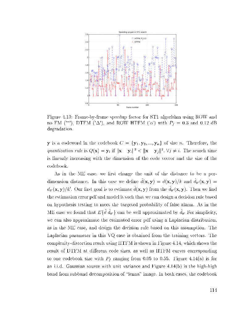
0 50 100 1500.8

1

1.2

1.4

1.6

1.8

2

2.2

2.4

2.6Speeding up gain in ST1 search

frame number

:HTFM, Pf 0.3

:DTFM

Figure 4.13: Frame-by-frame speedup factor for ST1 algorithm using ROW and

no FM ('*'), DTFM ('�'), and ROW HTFM ('o') with Pf = 0.3 and 0.12 dB

degradation.

y is a codeword in the codebook C = fy1;y2; :::;yng of size n. Therefore, the

quantization rule is Q(x) = yi if kx� yik2 < kx� yjk2, 8j 6= i. The search time

is linearly increasing with the dimension of the code vector and the size of the

codebook.

As in the ME case, we �rst change the unit of the distance to be a per-

dimension distance. In this case we de�ne ~d(x;y) = d(x;y)=k and ~dk0(x;y) =

dk0(x;y)=k0. Our �rst goal is to estimate ~d(x;y) from the ~dk0(x;y). Then we �nd

the estimation error pdf and model it such that we can design a decision rule based

on hypothesis testing to meet the targeted probability of false alarm. As in the

ME case we found that Ef ~dj ~dk0g can be well approximated by ~dk0 For simplicity,

we can also approximate the estimated error pdf using a Laplacian distribution,

as in the ME case, and design the decision rule based on this assumption. The

Laplacian parameter in this VQ case is obtained from the training vectors. The

complexity-distortion result using HTFM is shown in Figure 4.14, which shows the

result of DTFM at di�erent code sizes, as well as HTFM curves corresponding

to one codebook size with Pf ranging from 0.05 to 0.55. Figure 4.14(a) is for

an i.i.d. Gaussian source with unit variance and Figure 4.14(b) is the high-high

band from subband decomposition of \lenna" image. In both cases, the codebook

114

Table 4.1: Total time for encoding 150 frames and PSNR.

sequence FM ST1 Log ES

sec. PSNR sec. PSNR sec. PSNR

128 pels 37.78 32.4619 43.79 32.1536 472.75 32.3670

DTFM (128 pels) 35.42 32.4619 39.33 32.1536 152.37 32.3670

DTFM (64 pels) 33.63 32.1194 35.54 31.3711 98.25 31.9531

DTFM (32 pels) 32.58 31.9322 33.59 30.9696 71.05 31.6990

HTFM 20% 34.44 32.4518 35.14 32.1612 84.59 32.36

HTFM 30% 33.78 32.4218 34.50 32.1436 80.39 32.3385

mobile

HTFM 40% 33.52 32.3548 34.11 32.0778 77.88 32.2721

128 pels 39.05 40.4285 44.72 40.0528 449.64 40.5188

DTFM (128 pels) 37.75 40.4285 42.19 40.0528 231.80 40.5188

DTFM (64 pels) 34.40 40.2436 36.34 39.7743 129.63 40.3235

DTFM (32 pels) 32.69 40.1621 33.62 39.6797 88.31 40.2269

HTFM 20% 36.39 40.3264 36.70 39.8961 102.43 40.4645

HTFM 30% 35.16 40.2576 35.64 39.8524 93.38 40.4341

football

HTFM 40% 34.25 40.1938 34.92 39.7897 87.94 40.3937

128 pels 37.75 35.3020 44.67 34.6225 466.02 35.3124

DTFM (128 pels) 35.75 35.3020 40.69 34.6225 148.64 35.3124

DTFM (64 pels) 33.19 35.0397 35.71 33.7696 94.88 35.0197

DTFM (32 pels) 32.37 34.9337 33.41 33.2857 68.80 34.9056

HTFM 20% 34.67 35.2834 35.81 34.6291 92.80 35.2976

HTFM 30% 34.00 35.2499 35.24 34.6072 87.78 35.2548

ower

HTFM 40% 33.50 35.1884 34.66 34.5820 82.23 35.1661

is designed using the LBG [104] algorithm from training vectors which are i.i.d.

Gaussian and typical images, respectively.

We can see that unlike the ME case, in which the equivalent codebook size

is �xed by the search region, in this VQ case the size of the codebook can be

chosen to meet a complexity-distortion requirement. Note, however, that in order

to operate in a computation scalable mode, in the DTFM case the codebook size

has to be modi�ed, while scalability is achieved with a constant codebook size for

the HTFM case. In Figure 4.14, complexity-distortion performance achieved by

HTFM is approximately the same as that achieved with DTFM using di�erent

codebook size within a certain range. This is due to several factors. First, the

115

Table 4.2: cont. Total time for encoding 150 frames and PSNR.

sequence FM ST1 Log ES

sec. PSNR sec. PSNR sec. PSNR

128 pels 42.61 35.0416 47.30 35.27 464.34 35.01

DTFM (128 pels) 40.67 35.0416 43.34 35.00 175.66 35.01

DTFM (64 pels) 37.96 34.9403 39.26 34.8811 107.44 34.9068

DTFM (32 pels) 36.77 34.9051 37.37 34.8461 77.58 34.8624

HTFM 20% 39.21 35.01 39.30 34.9610 92.25 35.00

HTFM 30% 38.31 34.9662 38.60 34.9319 86.29 34.9879

cheer

HTFM 40% 37.66 34.9219 37.85 34.9011 83.32 34.9712

128 pels 42.28 35.1687 47.58 34.4392 461.28 35.1983

DTFM (128 pels) 40.47 35.1687 45.04 34.4392 224.13 35.1983

DTFM (64 pels) 36.78 34.8938 38.99 34.0651 128.43 34.8431

DTFM (32 pels) 35.06 34.7540 36.16 33.9563 87.87 34.6779

HTFM 20% 37.66 34.9628 39.56 34.3932 102.76 35.1574

HTFM 30% 36.89 34.8585 38.42 34.3518 93.73 35.1083

bicycle

HTFM 40% 36.18 34.7495 37.53 34.2934 87.95 35.0401

speedup from using DTFM alone is already large, i.e., about 3 to 4 times faster

than the original MSE computation. More than 90% of the distance computations

are terminated early by DTFM, and most of the terminations occur at early stages.

Second, the HTFM introduces more overhead cost for testing while providing

more early termination at �rst few stages. However, the number of additional

early termination is relatively small compared to the overall gain achieved by

DTFM. Finally, the vector dimension in VQ case is still far less than in the ME

case (16x16 macroblock). Thus, a few extra early terminations at an earlier stage

are outweighed by the overhead cost for extra testing. Therefore, in order to

get the maximum speedup performance, in our experiment for subband data VQ,

Figure 4.14(b), we apply the HTFM test to the �rst one quarter of dimensions

and simply use the DTFM test for the rest. As a conclusion, the HTFM for

VQ, even though it does not provide a signi�cant speedup over DTFM, provides

computational scalability for a given �xed codebook, while scalability can only be

achieved with di�erent codebook sizes with DTFM.

116

0.06 0.08 0.1 0.12 0.14 0.16 0.18 0.2 0.22 0.240.5

1

1.5

2

2.5

3

3.5

4

4.5

5x 10

8 Gaussian with σ2 = 1.0 vector size 8

MSE

Tot

al c

lock

cyc

le:DTFM

:N= 8192

: 6144

: 4096

: 2048

: 1024

(a)

7 7.5 8 8.5 9 9.5 10 10.50

1

2

3

4

5

6

7

8

9

10x 10

7 Distortion−Complexity of HH band "lenna" vector size 4x4

tota

l clo

ck c

ycle

MSE

: DTFM

:N=8192

: 4096

: 2048

: 1024

(b)

Figure 4.14: Complexity-distortion of HTFM VQ with vector size (a) 8 for i.i.d.

source and (b) 16 (4x4) for high-high band of \lenna" image.


To summarize the HTFM, we propose a fast motion estimation by using fast

matching in variable complexity framework where the number of pixels used in

calculation varies depending on the likelihood that the MAD which is estimated

by partial MAD will be larger than the \best found-so-far" SAD. The complexity

is input-dependent i.e. it varies depending on the nature of sequences, and is

adjustable by the degree of probability to make wrong decision. We formalize

the problem with the assumption of the knowledge of the distribution of the

MAD estimation error. Then the hypothesis testing is applied to minimize the

probability of error. We call this novel algorithm HTFM.

We can apply HTFM to the matching criterion computation of any FS algo-

rithm and also the nearest neighbor search for VQ encoding. However, in the case

of ME the complexity reductions as observed from our experiment are less when

more eÆcient FS is used because the set of considered MVs becomes so highly

competitive that it is more diÆcult to predict which vector would win. Neverthe-

less, with a fast search algorithm we still achieve signi�cant complexity reduction

e.g., 45% with 0.1 dB PSNR degradation of the reconstructed sequences for 2-D

Log search whereas we get 65% complexity saving for ES case. Therefore, our

117

algorithm allows a complexity-distortion tradeo� in fast matching that was not

achieved by previous work. For example, in [67], attempts to reduce the complex-

ity are done with reduced but �xed complexity algorithm, i.e. the complexity is

not input-dependent. We also show the result of using reduced subset fast match-

ing with DTFM. However, our HTFM still performs better. While other authors

[86] have studied variable complexity approaches, these were targetting the C-D

trade-o� in FS, rather than FM as we propose.

118

Chapter 5

Motion Estimation: PDS-based

Candidate Elimination

In this chapter we propose algorithms that perform both FM and FS approaches

for motion estimation simultaneously using the technique of PDS-based candidate

elimination. Similar to the HTFM in Chapter 4, this approach is based on the par-

tial distance search (PDS) [79] in which the SAD calculation is broken into several

steps, and at each step the partial SAD is updated and the calculation is allowed

to stop once it is clear that the SAD will be greater than the best-so-far SAD.

However, in the proposed approach, instead of using the PDS algorithm to pro-

vide early termination of SAD computation of candidates evaluated sequentially,

in this work, SAD of several candidates are computed simultaneouly step-by-step

and at each step some of them are eliminated from the pool of candidates based

on their potential to become the best candidate. The proposed algorithm can be

viewed as a path search algorithm where the goal is to �nd a path with minimal

SAD which represents the best candidate. Unlike the HTFM in Chapter 4, we do

not have a model of the relationship between the partial and the full SAD. We

use a simpler threshold for the likelihood testing. In addition, we also propose a

multiresolution approach in which the spatial dependency is used to help reduce

the number of candidates considered in early stages. Only few candidates consid-

ered as representatives of their neighbors are evaluated. If these representatives

show the tendency to be good motion vectors, their neighbors will be evaluated

119

next. We propose two variants of the multiresolution approach, i.e., breadth-�rst

and depth-�rst algorithms, respectively.

This chapter is organized as follows. In Section 5.1, we propose the ideal

dynamic programming which achieves minimal complexity in terms of arithmetic

operations. In Section 5.2, faster, albeit, suboptimal, variations of the multiple

step PDS approach are proposed. In Section 5.3, the multiresolution algorithms

are presented. The complexity-distortion results of all the proposed algorithms

are also shown in this section. The conclusions are drawn in Section 5.4.

5.1 PDS-based Candidate Elimination

The complexity reduction from the PDS when applying to various search strategies

can vary widely (e.g. 10-80%) depending on two major factors, namely, (i) how

the macroblock B is partitioned, and (ii) what fast search (FS) algorithm is used.

In the HTFM approach of Chapter 4, we propose a uniform partition (UNI) as a

better method for macroblock partitioning as compared to row-by-row partition

(ROW) in that it requires fewer pixel comparisons on the average. Therefore, in

this work, we will also use the UNI scheme. In this chapter we also provide some

experimental results on H.263 sequences in which we calculate the SAD using up

to 256 pixel instead of 128 pixel as in the MPEG2 case in Chapter 4 (Fig. 4.1).

The UNI partitioning for H.263 sequences is thus shown in Fig. 4.1.

In order to better visualize the e�ect of macroblock partitioning and associated

FS algorithm, the cumulative probability of early termination in a 16-stage PDS

is shown in Figure 5.2. The cumulative probability is de�ned as

Ft(i) = Prft � ig

where t is the stage in which the termination occurs, and t = 1; 2; :::; 16. From

Figure 5.2, the average number of stages required before the PDS termination

can be easily seen from the area above each curve, Eftg =R(1� Ft(i))di. This

average termination stage varies from sequence to sequence. Furthermore, it can

be seen from the �gure that the average termination stage using UNI is less than

120

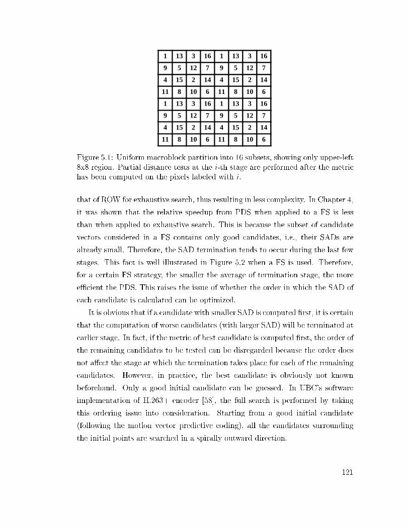
1 13 3 16 1 13 3 16

9 5 12 7 9 5 12 7

4 15 2 14 4 15 2 14

11 8 10 6 11 8 10 6

1 13 3 16 1 13 3 16

9 5 12 7 9 5 12 7

4 15 2 14 4 15 2 14

11 8 10 6 11 8 10 6

Figure 5.1: Uniform macroblock partition into 16 subsets, showing only upper-left

8x8 region. Partial distance tests at the i-th stage are performed after the metric

has been computed on the pixels labeled with i.

that of ROW for exhaustive search, thus resulting in less complexity. In Chapter 4,

it was shown that the relative speedup from PDS when applied to a FS is less

than when applied to exhaustive search. This is because the subset of candidate

vectors considered in a FS contains only good candidates, i.e., their SADs are

already small. Therefore, the SAD termination tends to occur during the last few

stages. This fact is well illustrated in Figure 5.2 when a FS is used. Therefore,

for a certain FS strategy, the smaller the average of termination stage, the more

eÆcient the PDS. This raises the issue of whether the order in which the SAD of

each candidate is calculated can be optimized.

It is obvious that if a candidate with smaller SAD is computed �rst, it is certain

that the computation of worse candidates (with larger SAD) will be terminated at

earlier stage. In fact, if the metric of best candidate is computed �rst, the order of

the remaining candidates to be tested can be disregarded because the order does

not a�ect the stage at which the termination takes place for each of the remaining

candidates. However, in practice, the best candidate is obviously not known

beforehand. Only a good initial candidate can be guessed. In UBC's software

implementation of H.263+ encoder [58], the full search is performed by taking

this ordering issue into consideration. Starting from a good initial candidate

(following the motion vector predictive coding), all the candidates surrounding

the initial points are searched in a spirally outward direction.

121

0 2 4 6 8 10 12 14 160

0.1

0.2

0.3

0.4

0.5

0.6

0.7

0.8

0.9

1Cumulative prob. of termination

stage number

:foreman

:miss_am

:salesman

:mthr_dotr

:suzie

solid : ROW

dashed: UNI

dash−dotted: FS & UNI

Figure 5.2: Cumulative probability of termination using 16 stage PDS and ex-

haustive search with ROW ('solid') and UNI ('dashed'), and using TMN's fast

motion search with UNI ('dash-dotted') of 150 frames of �ve H.263 sequences

coded at 56 Kbps. The eÆciency of the PDS relatively drops as a FS is used.

5.1.1 Ideal Candidate Elimination

The dynamic programming is proposed as one way to achieve the minimal number

of pixel comparison operations, which would correspond to the case when as if

the best candidate is evaluated �rst. The basic idea of the ideal elimination is to

update only a candidate with the smallest value of the partial SAD (PSAD) at a

time. Using the same notation as in Chapter 4, the ideal candidate elimination

algorithm is summarized as follows.

Algorithm 6 (Ideal Candidate Elimination (ICE-PDS))

Step 1:Set SAD� to in�nity. Compute the PSAD1 of every candidate in the

search region. Set the stage index, n(i), of every candidate to one, i.e., n(i) = 1

for all i candidates.

Step 2:Select candidate, i�, with smallest value of PSAD satisfying i) PSAD <

SAD� and ii) n(i�) < 16. If no such candidate exists, return with the SAD� result.

Step 3:Compute PSADn(i�)+1 of this candidate. Set n(i�) = n(i�) + 1.

Step 4:If n(i�) = 16, compare the PSAD with SAD� and select the minimal

to be the next SAD� and the corresponding best-so-far MV, ~MV�.

122

Step 4:Repeat Step 2.

It can be veri�ed that with this method, every candidate is terminated as earliest

as possible since the PSAD will remain not updated as long as it is not the minimal

PSAD at any given time. However, this algorithm requires multiple access to

each of the candidates as well as determining the one with minimal PSAD at each

step. These two overhead components may result in higher complexity than for

the sequential candidate evaluation approach.

5.1.2 Reduced Steps Candidate Elimination

One way to reduce the amount of overhead mentioned above is to limit the number

of times each candidate is considered. This is done by reducing the number of

stages at which the PSAD calculation can be stopped. In this chapter, we propose

a two-step CE-PDS. In the �rst step we compute the partial SAD of all candidates

up to stage m. Then the candidate with minimal PSADm is predicted to be the

best vector and therefore its SAD is computed �rst by continuing SAD calculation

from stage m. Then other candidates' SADs are computed using the PDS. Note

that we can also apply the PDS technique in the �rst step. The stage number

where termination occurs in the �rst step (Step 1 of Algorithm 7), n(j), must be

kept as the starting point from which the second step SAD calculation takes o�.

The algorithm is summarized as follows.

Algorithm 7 (Two-Step Candidate Elimination (2-CE-PDS))

Step 1: With a preselected m value, �nd MV �(�; xm) using PDS and keep

the partial SAD, SAD( ~mvj; xn(j)) where n(j) � m is de�ned above for the j-th

candidate.

Step 2: Update SAD(MV �(�; xm); B) �rst, set it to SADbsf and use PDS to

compute SAD( ~mvj; B) 8j; ~mvj 6=MV �(�; xm), starting from PSADn(j).

This method does not employ an initialization technique like other FS al-

gorithms. It is based solely on the matching metric. With this algorithm, the

memory corresponding to the search area has to be accessed only twice. In Ta-

ble 5.1, the complexity in terms of the number of stages in the SAD calculation (or

123

equivalently, number of pixel comparison operation) of the 2-CE-PDS algorithm

is shown and compared with the original PDS and the ideal PDS in which the

best candidate is found �rst. Note that all algorithms result in the same rate-

distortion performance. The experiment is based on UBC's TMN version 3.2 [58].

The experimental environment is as follows, 56 Kbps target bit rate, code �rst

150 frames of each sequence, search distance 5x5 around the initial guess (o�set)

motion vector, code I and P-frame only, and use full search1. There are 16 stage

in computing SAD as in Figure 5.1. The complexity in the unit described above

reduces from the original PDS with UNI by the amount of 0.5-5% when m = 1

as compared to the ideal PDS complexity reduction which is about 1-7.5%.

Table 5.1: Number of PSAD metric computation stages for di�erent PDS variation

for 150 frames of H.263 sequences coded at 56 Kbps.H.263 Orig. PDS Orig. PDS Ideal PDS 2-CE-PDS

sequences (ROW) (UNI) (UNI) m = 1 mmin

miss am 3214159 3015848 2944313 2962825 2955141

foreman 3528755 3407654 3151037 3222447 3181377

salesman 2355461 2166800 2144171 2154860 2150489

mthr dotr 2975387 2725827 2680578 2700361 2690790

suzie 3930649 3740283 3585322 3618637 3596301

Figure 5.3 shows the complexity of the 2-CE-PDS algorithm with di�erent

values of m. The value of m controls the tradeo� between the complexities of the

computations before and after them-th stage. Clearly, ifm is small, we have a less

accurate guess of the best candidate, whereas ifm is large, we get a good guess but

spend more on computation in the �rst step. However, with the optimal value of

m, mmin, the minimal complexity is just less than 1% over the ideal PDS result for

all sequences. The value of mmin for \Miss America", \Foreman", \Salesman",

\Mother&Daughter", \Suzie" are 5, 5, 8, 8 and 4, respectively. The value of

mmin can be related to the cumulative probability of termination in Fig. 5.2.

In sequences where the initial candidate is not good enough, the termination

can occur at any stage (see \Suzie") whereas with good initial candidate the

termination tends to be seen earlier (see \Salesman"). With the former type

1The processor type is Pentium II 450 MHz with Windows NT 4.0.

124

of sequences, the �rst step PDS signi�cantly helps reducing the complexity by

�nding a good guess of initial candidate. For the latter type of sequences where

the initial \guess" is good enough, in order to get even better initial candidate,

the number of stages m needs to be larger. However, the di�erence between the

original PDS (UNI) and the ideal PDS is already small (from 1-10%) because

of the good initial candidate provided by the original algorithm, thus using any

small value of m yields similar results. Therefore, for simplicity, m = 1 would be

a good choice.

0 5 10 152.94

2.95

2.96

2.97

2.98

2.99

3

3.01

3.02x 10

6

m

com

plex

ity

"miss_am" result of two stage PDS

(a)

0 5 10 153.58

3.6

3.62

3.64

3.66

3.68

3.7

3.72

3.74

3.76x 10

6

m

com

plex

ity

"suzie" result of two stage PDS

(b)

Figure 5.3: Complexity (number of stages) versus m for (a) \Miss America" and

(b) \Suzie". The top and bottom lines in each �gure are the original PDS with

UNI and the ideal PDS, respectively.

One can further generalize the two-step algorithm to an algorithm having an

arbitrary number of step (P-CE-PDS), i.e., we divide the calculation into p steps,

for each step we update the best partial SAD �rst. Letm(i), i = 1; :::; p, denote the

SAD calculation stage at which step i stops, and m(1) < m(2) < ::: < m(p) = b,

i.e., xm(p) = B. The p-step PDS can be written as

Algorithm 8 (P-Step Candidate Elimination (P-CE-PDS))

Step 1: Assume there are p steps to compute SAD. The i-th step stops at

stage m(i), i = 1; ::; p. Set i = 1

Step 2: FindMV �(�; xm(i)) using PDS and keep the partial SAD, SAD( ~mvj; xn(j))

where n(j) � m(i) for the j-th candidate.

125

Step 3: Compute SAD(MV �(�; xm(i)); xm(i+1)) �rst, set it to SADbsf and

�nd MV �(�; xm(i+1)) using PDS by computing SAD( ~mvj; xm(i+1)) for other j-th

candidate starting from PSADn(j).

Step 4: i = i + 1. If i < p repeat Step 3. Otherwise, return MV �(�; B).

When the number of the steps of the P-PDS is equal to number of steps of

the PDS, this algorithm is equivalent to the ICE-PDS in Algorithm 6. However,

from our preliminary result the additional speedup using P-CE-PDS does not

signi�cantly improve 2-CE-PDS results. Also, it can be seen that even with the

ideal PDS, the additional speedup is small when the original algorithm already

starts with a good initial candidate, as in our experiment. In order to achieve

further complexity reduction, we have to resort to a fast search which may not

reach a global minimum vector.

5.2 Suboptimal CE-PDS

In this section, we further motivate a suboptimal solution using the result of the

CE-PDS algorithms. Unlike other FS algorithms, which have an assumption of

monotonically increasing error surface as the distance between a candidate and the

local minimum grows, we reduce the number of the candidates tested using their

own partial metric information. The key idea would be analogous to a tree growing

where only a few branches are kept at a given stage. We propose 2 techniques to

limit the number of branches grown, one is computationally nonscalable and the

other is computationally scalable.

5.2.1 Computationally Nonscalable Fast Search

We start with an example on 2-CE-PDS. In the Step 2 of Algorithm 7 we up-

date the SAD of candidates whose PSADm has been computed, i.e., for those

candidates terminated before stage m, the SAD computation is never completed.

This makes sense because it is likely that candidates surviving the �rst step PDS

will be good candidates. We can then generalize this idea to p-step which can be

summarized as follows using the same notation as previously.

126

Algorithm 9 (P-Step Fast CE-PDS (P-FCE))

Step 1: Assume there are p steps to compute SAD. The i-th step stops at

stage m(i), i = 1; ::; p, and xm(p) = B. Set i = 1, and 1 = �.

Step 2: Find MV �( 1; xm(i)) using PDS and keep the partial SAD of the j-th

candidate, SAD( ~mvj; xn(j)), only for those whose n(j) = m(i).

Step 3: Update SAD(MV �( i; xm(i)); xm(i+1)) �rst, set it to SADbsf .

Step 4: Let i+1 = f ~mvjjn(j) = m(i)g. Find MV �( i+1; xm(i+1)) using PDS

by updating SAD( ~mvj; xm(i+1)) 8j. Update n(j).Step 5: i = i + 1. If i < p repeat Step 3. Otherwise, return MV �( p; xm(p)).

Table 5.2: Results of 2-FCE complexity reduction with respect to the original

PDS.Sequences SNR mmin Complexity % comp. CPU clk. % clk.

di�erence (# stages) reduction cycle ratio reduction

miss am 0 dB 3 1030878 67.9% 1853/3277 43.5%

foreman -0.01 dB 4 1566098 55.6% 2157/3719 42.0%

salesman 0 dB 3 808212 65.7% 1545/2687 42.5%

mthr dotr +0.01dB 3 1049889 64.7% 1807/3108 41.9%

suzie +0.02dB 4 1695524 56.9% 2362/3607 34.5%

The intrinsic complexity of this algorithm stems from having to test whether

a candidate is quali�ed for the next step PSAD computation or not. As there

are more steps, this cost becomes larger and may outweigh the reduction of pixel

comparisons. Therefore, similar to the discussion in the previous section, only

2-step FCE is considered. In Table 5.2, the result of 2-FCE with optimal value of

m is shown. It can be seen that the complexity reduction, in terms of number of

stages and the actual execution time, is obviously promising, with near optimal

motion search performance.

Table 5.3 shows the result of 8-Step FCE with 2 stage interval between steps.

We can see that the number of stage operation is further reduced but the total

CPU clock cycle increases by 1-5% because of more testing operations overhead

for valid candidates in each step. Therefore, our conclusion is that using 2 step

suÆces for signi�cant speedup gain in terms of the execution time.

Table 5.4 shows the result of the fast search implemented in TMN H.263

codec [58]. It can be seen that even though our algorithm shows near optimal

127

Table 5.3: Results of 8-FCE (2 stage PSAD per 1 step testing).

Sequences SNR Complexity % comp. CPU clk. % clk.

di�erence (no. of stages) reduction cycle ratio reduction

miss am +0.01 dB 811838 74.7% 1983/3277 39.5%

foreman -0.04 dB 1055540 70.1% 2145/3719 57.7%

salesman 0 dB 663683 71.8% 1740/2687 35.2%

mthr dotr -0.01dB 796422 73.2% 1889/3108 39.2%

suzie -0.01dB 1142971 70.9% 2187/3607 39.4%

Table 5.4: Result of using UBC's Fastsearch option.

Sequences SNR Complexity %comp. CPU clk. % clk.


miss am -0.02 1139316 64.5% 1689/3277 48.5%

foreman -0.11 1225935 65.3% 1702/3719 54.2%

salesman 0 816724 65.3% 1399/2687 47.9%

mthr dotr -0.05 1004437 66.2% 1543/3108 50.4%

suzie -0.04 1267551 67.8% 1749/3607 51.5%

performance and less number of stage computation, in terms of execution time our

algorithm is a bit inferior. This is due to extra clock cycles spent on candidates

testings before computing the next step PSAD and multiple memory access for

the search area. Another disadvantage of this algorithm is that the complexity

is not scalable, i.e., the complexity-distortion operating point is �xed. Therefore,

in order to be able to compare the performance with UBC's fast search at the

same execution time or same distortion, we resort to a computationally scalable

solution which allows signi�cant speeding up gain with the sacri�ce in some quality

degradation.

5.2.2 Computationally Scalable Fast Search

To further reduce the complexity, we can limit the number of candidates passing

to the next stage either by comparing the PSAD with a threshold or selecting only

a limited number of candidates with the least PSAD. In this work, we choose to

128

follow the �rst approach because of simplicity in implementation. If the second

approach is to be used, an extra complexity for sorting must be taken into account

which will lessen the overall speedup. Consider the 2-step algorithm, after the �rst

step we have an information of the best partial metric. Also, after updating the

best partial SAD to obtain SADbsf , we can surmise that the �nal SAD would

have the value around (strictly equal or less) the SADbsf . We can then set up a

threshold with the value proportional to the SADbsf and the number of stage left

in the 2nd step. Speci�cally, the threshold, T , is de�ned as

T = t � SAD(MV �(�; xm); B) �m=16

where t is a control parameter to adjust the tradeo� between the complexity

and quality. The threshold is proportional to the linearly scaled version of the

best-so-far SAD. Unlike Algorithm 7, in this scheme we only test for the PSAD

thresholding. We do not test the value of n(j), in order to maintain a reasonable

complexity. In fact, for t less than or equal to 1, all the candidates that do not

survive the �rst step PDS will also fail the threshold testing. For t greater than

1, the scheme allow more candidates to be considered even if they fail the �rst

stage PSAD.

The computationally scalable algorithm can be summarized as follows.

Algorithm 10 (2-Step with Threshold Fast CE-PDS (2T-FCE))

Step 1: FindMV �(�; xm) using PDS and keep the partial SAD, SAD( ~mvj; xn(j))

8 ~mvj 2 � where n(j) � m for the j-th candidate.

Step 2: Update SAD(MV �(�; xm); B) �rst, set it to SADbsf and �ndMV �( ; B)

using the PDS where = f ~mvjjSAD( ~mvj; xn(j)) < Tg where n(j) is the startingstage for candidate j.

Note that this 2-step algorithm can be easily extended to a p-step version.

Table 5.5 shows the result of applying Algorithm 10 with m = 1 and t = 1. One

can see that in most cases, we perform better than the UBC's fast search algorithm

in both SNR and complexity (both execution time and number of operations).

Besides, our algorithm is computationally scalable, i.e., the complexity can be

made smaller by adjusting t to be smaller. As a result of smaller t, the quality

129

Table 5.5: Result of 2-Step with Threshold when m = 1 and t = 1.

Sequences SNR Complexity %comp. CPU clk. % clk.


miss am -0.02 647465 79.9% 1505/3277 54.1%

foreman -0.08 839797 76.2% 1655/3719 55.5%

salesman -0.03 581914 75.3% 1488/2687 44.6%

mthr dotr -0.02 657439 77.9% 1524/3108 50.9%

suzie +0.01 831575 78.8% 1621/3607 55.1%

will be slightly degraded. Examples of the complexity-distortion behavior of the

algorithm will be provided in the next section.

5.3 Multiresolution Algorithm

The proposed CE-PDS algorithm can be viewed as a variance of multiresolution

algorithm (see [75], [77], etc.) where the pyramid decomposition and subsampling

without anti-aliasing �lter are used2. In general, the variable block size multires-

olution algorithm can be implemented using the PDS technique. In the simplest

scheme where no �ltering operation is performed prior to subsampling, the coars-

est resolution motion search is equivalent to searching over a subsampled grid

of pixel using PSADn such that xn correspond to the subsampled pixels in the

lowest resolution. In a �ner resolution, the center of the search is obtained from

the result of the coarser resolution search and the e�ective search area in the �ner

resolution can be reduced. The PSAD of candidates on the grid of �ner resolution

are then evaluated using a corresponding subset of pixel. The coarsest resolution

grids come from the set of pixels in the �rst set of the UNI partitioning. Each

set of pixels can be considered as one polyphase of the data. A �ner resolution

consists of more polyphases than a coarser resolution.

However, one advantage of the original multiresolution approach is the use of

correlation between matching metrics of adjacent motion vectors to speedup the

2As discussed in [77] lack of an anti-aliasing �lter is not crucial in pyramid coding.

130

search. In our algorithms in previous sections, this fact is not taken into con-

sideration, thus resulting in redundant computations for candidates in the same

neighborhood with similar matching metric values. Therefore, in this section, we

propose algorithms that in addition to allowing scalable complexity based on our

previous method, also take advantage of the candidate vector correlation as in the

conventional multiresolution approach. There are several ways to obtain compu-

tational scalability. For example, the constraint of �nding the best candidate in a

particular resolution can be loosened in such a way that a \good" but not optimal

candidate can be chosen if it can be found much faster than the optimal one. An

approach is to allow more than one candidate to be the center of the search in

the �ner resolution using the partial metric criterion. This can be viewed as a

soft-decision on what the initial candidate should be in the next resolution. We

use a threshold approach similar to Algorithm 10 where the threshold is computed

�rst from the initial motion vector at the center of the search region in the �nest

resolution. At the coarsest resolution, we compute the �rst stage PSAD on the

coarsest grid. Candidates with PSAD less than the �rst threshold are then con-

sidered for the next step/resolution PSAD, as well as their neighbors in the �ner

resolution.

The order of the search in �ner resolutions can be performed by a breadth-�rst

or a depth-�rst approach. In breadth-�rst, the update of the partial metrics is per-

formed for all candidates in the next level �rst before continuing to the following

level. In depth-�rst, there are only two steps in partial metric computation, i.e.,

the update of partial metric is from the current resolution to the �nest resolution.

We propose two algorithms in Algorithm 11 and 12 corresponding to the breadth-

�rst and depth-�rst approaches, respectively. Prior to describing the algorithm,

let us introduce some new notations. Let us assume that there are R levels of

resolution. Each resolution is obtained from subsampling the �ner resolution by

a factor of four. The macroblock is thus partitioned such that x1 consists of only

pixels in the coarsest resolution and there exist xn(r) for resolution r such that

pixels in xn(r) correspond to pixels in resolution r (n(1) = 1). In our experiment

for H.263 sequences, there are 3 resolutions and n(1) = 1; n(2) = 4,and n(3) = 16

(refer to Figure 5.1). Let r be the set of candidates on the subsampled grid at

131

the r-th resolution. Let �r( ~mv) be the set of motion vectors in the neighbor-

hood of ~mv in the r-th resolution, i.e., they are ~mv + [�2R�r;�2R�r] where Ris the level number of the �nest resolution. From these notations, the proposed

multiresolution (MR) algorithms can be summarized as follows.

Algorithm 11 (Breadth-First Multiresolution (MR1-FCE))

Step 1:Find the SAD of the initial motion vector, set it to SADbsf . Compute

T (r) for r = 1; :::; R from T (r) = SADbsf � 1=4(R�r) � t. Set r = 1.

Step 2:Compute SAD( ~mv; x1) using PDS, 8 ~mv 2 1. r r + 1.

Step 3:If SAD( ~mv; xn(r�1)) < T (r�1), i) use PDS to update to SAD( ~mv; xn(r))

and ii) compute the neighboring SAD(~v; xn(r)) using PDS 8~v 2 �r( ~mv).Step 4:r r + 1. If r < R, repeat step 3. Otherwise, go to step 5.

Step 5:If SAD( ~mv; xn(R�1)) < T (R�1), i) use PDS to update to SAD( ~mv; xn(R))

and ii) compute SAD(~v; xn(R)) using PDS 8 ~v 2 �R( ~mv).Step 6:Return MVbsf as the best motion search result.

Algorithm 12 (Depth-First Multiresolution (MR2-FCE))

Step 1:The same as Step 1 in MR1-FCE.


Step 3:If SAD( ~mv; xn(r�1)) < T (r�1), i) use PDS to update to SAD( ~mv; xn(R))

and remove ~mv from the list of the candidate to be processed, and ii) compute the

neighboring SAD(~v; xn(r)) using PDS 8 ~v 2 �r( ~mv) .Step 4:r r + 1. If r < R, repeat step 3. Otherwise, go to step 5.


In both algorithms, the SADbsf and MVbsf are updated with the PDS at

the �nest resolution. In MR2-FCE, the number of steps for SAD calculation for

each candidate is at most two since the update is always to the �nest resolution.

The advantage of this approach is less number of data access (only twice) but

the computation could be higher for some candidates which have small PSAD at

early stages and large PSAD at later stages.

In Table 5.6, the result of the proposed multiresolution algorithms are shown

for t = 1:0 and compared with the conventional multiresolution algorithm that

use only one candidate as initial point in each resolution. It can be seen that

132

Table 5.6: Results of MR1-FCE and MR2-FCE complexity reduction at t = 0:8

with respect to the original multiresolution algorithm.

MR1-FCE MR2-FCE

Sequences SNR % clk. SNR % clk.

di�erence increase di�erence increase

miss am +0.31 dB 29.1% +0.32 dB 23.7%

foreman +0.73 dB 44.1% +0.82 dB 51.8%

salesman +0.04 dB 37.9% +0.04 dB 27.6%

mthr dotr +0.29 dB 25.7% +0.28dB 19.6%

suzie +0.56 dB 22.2% +0.56 dB 18.9%

the SNR is improved with the cost of extra computation. However, our proposed

algorithm is also computationally scalable.

0.4 0.45 0.5 0.55 0.6 0.65 0.7 0.75 0.8−0.09

−0.08

−0.07

−0.06

−0.05

−0.04

−0.03

−0.02

−0.01

0

0.01Complexity−Distortion average over 5 test sequences

dB d

iffer

ence

from

orig

inal

normalized CPU clock cycle

:TMN FS

:2−FCE

:2T−FCE

:HTFM

:MR1−FCE

:MR2−FCE

Figure 5.4: Complexity-Distortion using various algorithms average over 5 test

sequences. The complexity unit is the clock cycles normalized by the original

ROW PDS.

As shown in Fig. 5.4 and 5.5, the complexity-distortion curves of these two

MR algorithms with varying t from 0.8 to 2 is compared with the scalable 2T-

FCE and the nonscalable method 2-FCE from Table 5.2. The UBC's fast search

[58], and the complexity scalable hypothesis testing fast matching (HTFM) are

133

also shown in the �gures. Note that the results of the conventional multiresolu-

tion algorithm do not �t in the range displayed in Figure 5.4. The experimental

environment is the same as before. The result is averaged over 5 test sequences

which are \Miss America", \foreman", \salesman", \mother & daughter", and

\suzie". One can see that 3 of our proposed algorithms (2T-FCE, MR1-FCE

and MR2-FCE) outperform the fast algorithm in TMN3.0 and the HTFM at low

quality-low complexity region. Furthermore, MR1-FCE and MR2-FCE perform

almost equally well. In particular, MR1-FCE performs better at low quality (lower

thresholds) while MR2-FCE performs better at high quality area (higher thresh-

olds). This is reasonable because at high thresholds, there are more candidates

passing to the �ner resolutions, thus resulting in more overhead if there are many

steps in PSAD calculation as in MR1-FCE. Compared to 2T-FCE, the proposed

MR algorithms do not signi�cantly achieve further speedup. This is due to the

small search distance limit which has been set to �5 from the initial candidate at

the �nest resolution, i.e., only �1 at the coarsest resolution. If the search area is

larger, the gain from MR approach will be clearer. The result in terms of num-

ber of pixel comparisons is shown in Figure 5.5. It can be seen that since this

measure does not take the other complexity such as data access, PSAD testing,

candidate selection, boundary checking, etc. into account, which contribute about

20% margin in the clock cycle measure.


We have presented a novel algorithm (PT-FCE) that takes advantage of the par-

tial metric information to determine which candidates are worth to be fully eval-

uated. This algorithm can be viewed as a generalized version of multiresolution

approach in the sense that the partial metric is obtained from a subset of pixel in

a macroblock that corresponds to a certain resolution, and at each resolution the

candidates to be considered are not necessary spatially related to the best can-

didate in the coarser resolution. Furthermore, the algorithm is computationally

scalable, i.e., the complexity can be adjusted to meet the computational constraint

with some sacri�ce on poorer motion estimation performance. The result shows

134

0.2 0.25 0.3 0.35 0.4 0.45 0.5 0.55 0.6 0.65−0.09

−0.08

−0.07

−0.06

−0.05

−0.04

−0.03

−0.02

−0.01

0

0.01Complexity−Distortion average over 5 test sequences

dB d

iffer

ence

from

orig

inal

normalized no. stage operation

:TMN FS

:2−FCE

:2T−FCE

:HTFM

:MR1−FCE

:MR2−FCE

Figure 5.5: Complexity-Distortion using various algorithms average over 5 test

sequences. The complexity unit is the the number of pixel comparisons normalized

by the original ROW PDS.

that in terms of complexity-distortion tradeo� this novel algorithm (2T-FCE) out-

performs the hypothesis testing algorithm (HTFM) with also less sophisticated

algorithm.

Then, we propose two algorithms (MR1-FCE and MR2-FCE) that also use the

spatial information in deciding the candidates to be evaluated. These algorithms

possess a similar parent-child relationship as in the pyramid-based multiresolution

approach without anti-aliasing �ltering. They thus take advantage of spatial

correlation of motion vectors to speedup the search. It also performs better than

the original multiresolution because it allows soft-decision to be made based on

partial metric. Thus, it is computationally scalable depending on the threshold

factor that control the complexity-distortion tradeo�. The result shows that this

approach performs little bit better than 2T-FCE. However, when the search area

becomes larger, the di�erence in performance will be more visible.

135

References

[1] W. Pennebaker and J. Mitchell, JPEG Still Image Data Compression Stan-

dard. Van Nostrand Reinhold, 1994.

[2] J. Mitchell, W. Pennebaker, C. E. Fogg, and D. J. LeGall, MPEG Video

Compression Standard. New York: Chapman and Hall, 1997.

[3] S. G. 16, \H.263 video coding for low bit rate communication," tech. rep.,

ITU-T, 1997.

[4] J. Chalidabhongse and C.-C. Kuo, \Fast motion vector estimation us-

ing multiresolution-spatio-temporal correlations," IEEE Trans.Cir.Sys. for

Video Tech., April 1997.

[5] T. M. Cover and J. A. Thomas, Elements of Information Theory. Wiley-

Interscience, 1991.

[6] M. Antonini, M. Barlaud, P. Mathieu, and I. Daubechies, \Image coding

using wavelet transform," IEEE Trans. on Image Proc., 1992.

[7] Wavelet and Subband Coding. Prentice Hall P T R, 1995.

[8] K. Ramchandran, Z. Xiong, K. Asai, and M. Vetterli, \Adaptive transforms

for image coding using spatially varying wavelet packets," IEEE Trans. on

Image Proc., 1996.

[9] Y. Shoham and A. Gersho, \EÆcient bit allocation for an arbitrary set of

quantizers," IEEE Trans. on Signal Proc., vol. 36, pp. 1445{1453, Sept.

1988.

[10] K. Ramchandran, A. Ortega, and M. Vetterli, \Bit allocation for dependent

quantization with applications to multiresolution and MPEG video coders,"

IEEE Trans. on Image Proc., 1994.

[11] L.-J. Lin and A. Ortega, \Bit-rate control using piecewise approximated

rate-distortion characteristics," IEEE Trans. on Circ. and Sys. for Video

Tech., 1998.

136

[12] C. Chrysa�s and A. Ortega, \EÆcient context-based entropy coding for

lossy wavelet image compression," in In Proc. of DCC'97.

[13] J. M. Shapiro, \Embedded image coding using zerotrees of wavelet coeÆ-

cients," IEEE. Trans. on Signal Processing, 1993.

[14] D. Taubman and A. Zakhor, \Multirate 3-D subband coding of video,"

IEEE Trans. on Image Proc., 1994.

[15] A. Said and W. A. Pearlman, \A new, fast, and eÆcient image codec based

on set partitioning in hierarchical trees," IEEE Trans. on Circ. and Sys. for

Video Tech., 1996.

[16] H.-J. Wang and C.-C. Kuo, \A multi-Threshold wavelet coder (MTWC) for

high �delity image compression," 1997.

[17] J. Li and S. Lei, \An embedded still image coder with rate-distortion opti-

mization," IEEE Trans. on Image Proc., 1999.

[18] B.-B. Chai, J. Vass, and X. Zhuang, \Signi�cant-linked connected compo-

nent analysis for wavelet image coding," IEEE Trans. on Image Proc., 1999.

[19] M. Crouse and K. Ramchandran, \Joint thresholding and quantizer selection

for transform image coding: Entropy-constrained analysis and applications

to baseline JPEG," IEEE Trans. on Image Proc., 1997.

[20] J. Li, J. Li, and C.-C. Kuo, \Layered DCT still image compression," IEEE

Trans. on Circ. and Sys. for Video Tech., 1997.

[21] G. J. Sullivan and R. L. Baker, \EÆcient quadtree coding of images and

video," in Proc. of ICASSP'91, 1991.

[22] M. J. Gormish, Source Coding with Channel, Distortion and Complexity

Constraints. PhD thesis, Stanford University, Mar. 1994.

[23] V. Goyal and M. Vetterli, \Computation distortion characteristics of block

transform coding," in Proc. of ICASSP'97, (Munich, Germany), Apr. 1997.

[24] K. Rao and P. Yip, Discrete Cosine Transform, Algorithms, Advantages,

Applications. Academic Press, 1990.

[25] T. N. N. Ahmed and K. R. Rao, \Discrete cosine transform," IEEE Trans.

on Computer, 1974.

[26] M. Narasimha and A. Peterson, \On the computation of the discrete cosine

transform," IEEE Trans. on Comm., 1978.

137

[27] J. J.-I. Hong, Discrete Fourier, Hartley and Cosine Transforms in Signal

Processing. PhD thesis, Columbia University, 1993.

[28] C. S. Wen-Hsiung Chen and S. Fralick, \A fast computational algorithm for

the discrete cosine transform," IEEE Trans. on Comm., 1977.

[29] A. Ligtenberg and M. Vetterli, \A discrete fourier/cosine transform chip,"

IEEE J. on Selected Areas in Comm., vol. SAC-4, pp. 49{61, Jan 1986.

[30] Z. Wang, \Fast algorithms for the discrete w transform and for the discrete

fourier transform," IEEE Trans. on Signal Proc., vol. ASSP-32, pp. 803{816,

Aug. 1984.

[31] B. Lee, \A new algorithm to compute the discrete cosine transform," IEEE

Trans. on Signal Proc., vol. ASSP-32, pp. 1243{1245, December 1984.

[32] P. Duhamel and H. H'Mida, \New 2n DCT algorithms suitable for VLSI

implementation," in Proc. of ICASSP'87, (Dallas), p. 1805, Apr 1987.

[33] C. Loe�er, A. Ligtenberg, and G. Moschytz, \Practical fast 1-D DCT al-

gorithms with 11 multiplications," in In Proc. of ICASSP'89.

[34] E. Feig and E. Linzer, \Discrete cosine transform algorithms for image data

compression," in Proc. of Electronic Imaging'90, p. 84, 1990.

[35] M. Vetterli, \Tradeo�s in the computation of mono and multi-dimensional

DCTs," tech. rep., Ctr. fo Telecommunications Research, Columbia Univer-

sity, June 1988.

[36] E. Feig and S. Winograd, \On the multiplicative complexity of discrete

cosine transform," IEEE Trans. on Information Theory, 192.

[37] H. R. Wu and Z. Man, \Comments on "fast algorithms and implementation

of 2-D discrete cosine transform," IEEE Trans. on Circ. and Sys. for Video

Tech., 1998.

[38] N. I. Cho and S. U. Lee, \A fast 4x4 DCT algorithm for the recursive 2-D

DCT,"

[39] E. Linzer and E. Feig, \New scaled DCT algorithms for fused MULTI-

PLY/ADD architectures," in Proc. of ICASSP'91, vol. 4, pp. 2201{2204,

1991.

[40] V. Srinivasan and K. J. R. Liu, \Vlsi design of high-speed time-recursive

2-D DCT/IDCT processor for video applications," IEEE Trans. on Circ.

and Sys. for Video Tech., 1996.

138

[41] Y. Arai, T. Agui, and M. Nakajima, \A fast DCT-SQ scheme for images,"

Trans. of IEICE, vol. 71, p. 1095, Nov 1988.

[42] C. W. Kok, \Fast algorithm for computing discrete cosine transform," IEEE

Trans. on Signal Proc., 1997.

[43] V. S. Dimitrov, G. A. Jullien, and W. C. Miller, \A new DCT algorithm

based on encoding algebraic integers," in Proc. of ICASSP'98.

[44] N. Merhav and V. Bhaskaran, \Fast algorithms for DCT-domain

image down-sampling and for inverse motion compensation," IEEE

Trans.Circ.Sys. for Video Tech., vol. 7, no. 3, pp. 458{475, June 1997.

[45] H. V. Sorensen and C. S. Burrus, \EÆcient computation of the dft with only

a subset of input or output points," IEEE Trans. on Signal Proc., 1993.

[46] \The independent JPEG's group software JPEG, version 6."

ftp://ftp.uu.net.

[47] A. Hossen and U. Heute, \Fast approximation DCT: Basic-idea, error anal-

ysis, application," in Proc. of ICASSP'97.

[48] S. Jung, S. Mitra, and D. Mukherjee, \Subband DCT: De�nition, analysis,

and applications," IEEE Trans. on Circ. and Sys. for Video Tech., 1996.

[49] J. Bao, H. Sun, and T. Poon, \Hdtv down-conversion decoder," IEEE Trans.

on Consumer Electronics, 1996.

[50] J. Song and B.-L. Yeo, \Fast extraction of spatially reduced image sequences

from MPEG-2 compressed video," IEEE Trans. on Circ. and Sys. for Video

Tech., 1999.

[51] J. B. Lipsher, \Asynchronous DCT processor core," Master's thesis, Univ.

of Cal. Davis.

[52] J. Winograd and S. Nawab, \Incremental re�nement of DFT and STFT

approximations," IEEE Signal Proc. Letters, 1995.

[53] W. K. Cham and F. S. Wu, \Compatibility of order-8 integer cosine trans-

forms and the discrete cosine transform," in Proc. of IEEE Region 10 Conf.

on Computer and Communication Systems, 1990.

[54] A. Gersho and R. M. Gray, Vector Quantization and Signal Compression.

Kluwer Acad. Pub., 1992.

139

[55] K. S. Wang, J. O. Normile, H. Wu, and A. A. Rodriguez, \Vector-

quantization-based video codec for software-only playback on personal com-

puters," Multimedia Systems 2(5), pp. 191{203, 1994.

[56] \MPEG video software decoder, v2.2."

http://bmrc.berkeley.edu/projects/mpeg/mpeg play.html.

[57] \vic:UCB/LBL video conferencing tool."

ftp://ftp.ee.lbl.gov/conferencing/vic/.

[58] C. University of British Columbia, \Tmn h.263+ encoder version 3.0,"

http://www.ee.ubc.ca

/image/h263plus/.

[59] K. Froitzheim and H. Wolf, \A knowledge-based approach to JPEG ac-

celeration," in Proc. of IS&T/SPIE Symp. on Electr. Imaging Science and

technology, (San Jose), Feb. 1995.

[60] E. Murata, M. Ikekawa, and I. Kuroda, \Fast 2D IDCT implementation

with multimedia instructions for a software MPEG2 decoder," in Proc. of

ICASSP'98.

[61] X. Bo and Z. Xulong, \A new algorithm for the implementation of h.263

video coding," IEEE Trans. on Circ. and Sys. for Video Tech., To appear.

[62] K.Lengwehasatit and A.Ortega, \Distortion/decoding time tradeo�s in soft-

ware DCT-based image coding," in Proc. of ICASSP '97, 1997.

[63] B. Girod and K. W. Stuhlm�uller, \A content-dependent fast DCT for low

bit-rate video coding," in Proc. of ICIP'98.

[64] I.-M. Pao and M.-T. Sun, \Modeling DCT coeÆcients for fast video encod-

ing," IEEE Trans. on Circ. and Sys. for Video Tech., 1999.

[65] K. Lengwehasatit and A. Ortega, \DCT computation with minimal average

number of operations," in Proc. of VCIP'97, (San Jose, CA), Feb. 1997.

[66] K.Lengwehasatit and A.Ortega, \DCT computation based on variable com-

plexity fast approximations," in Proc. of ICIP'98.

[67] B. Liu and A. Zaccarin, \New fast algorithms for the estimation of block

motion vectors," IEEE Trans.Cir.Sys. for Video Tech., vol. 3, pp. 148{157,

April 1993.

[68] J. Jain and A. Jain, \Displacement measurement and its application in

interframe image coding," IEEE Trans. on Comm., 1981.

140

[69] R. Srinivasan and K. Rao, \Predictive coding based on eÆcient motion es-

timation," IEEE Trans.Comm., vol. COMM-33, pp. 888{895, August 1985.

[70] R. Li, B. Zeng, and M. Liou, \A new three-step search algorithm for block

motion estimation," IEEE Trans.Circ.Sys. for Video Tech., vol. 4, pp. 438{

442, August 1994.

[71] L.-K. Liu and E. Feig, \A block-based gradient descent search algorithm for

block motion esitmation in video coding," IEEE Trans.Circ.Sys. for Video

Tech., vol. 6, pp. 419{422, August 1996.

[72] J. Y. Tham, S. Ranganath, and M. Ranganath, \A novel unrestricted center-

biased diamond search algorithm for block motion estimation," IEEE Trans.

on Circ. and Sys. for Video Tech., vol. 8, pp. 369{377, August 1998.

[73] M. Bierling, \Displacement estimation by hierarchical block matching," in

Proc. of VCIP'88.

[74] F. Dufaux and M. Kunt, \Multigrid block matching motion estimation with

an adaptive local mesh re�nement," in Proc. of VCIP'92.

[75] S. Zafar, Y. Q. Zhang, and B. Jabbari, \Multiscale video representation

using multiresolution motion compensation and wavelet decomposition,"

IEEE J. on Sel. Areas in Comm., 1993.

[76] Y. Q. Zhang and S. Zafar, \Motion-compensated wavelet transform coding

for color video compression," IEEE Trans. on Circ. and Sys. for Video Tech.,

1992.

[77] K. M. Uz, M. Vetterli, and D. J. LeGall, \Interpolative multiresolution

coding of advanced television with compatible subchannels," IEEE Trans.

on Circ. and Sys. for Video Tech., vol. 1, pp. 86{99, March 1991.

[78] J.-B. Xu, L.-M. Po, and C.-K. Cheung, \Adaptive motion tracking block

matching algorithm for video coding," IEEE Trans. on Circ. and Sys. for

Video Tech., vol. 9, pp. 1025{1029, October 1999.

[79] C.-D. Bei and R. M. Gray, \An improvement of the minimum distortion

encoding algorithm for vector quantization," IEEE Trans. on Comm., 1985.

[80] Y.-C. Lin and S.-C. Tai, \Fast full-search block-matching algorithm or

motion-compensated video compression," IEEE Trans. on Comm., 1997.

[81] Z.-L. He, K.-K. Chan, C.-Y. Tsui, and M. L. Liou, \Low power motion

estimation design using adaptive pixel truncation," in In Proc. of Int'l Symp.

on Low Power Electronics and Design 1997, pp. 167{172.

141

[82] B. Natarajan, V. Bhaskaran, and K. Konstantinides, \Low-

complexity block-based motion estimation via one-bit transforms," IEEE

Trans.Circ.Sys. for Video Tech., vol. 7, pp. 702{706, August 1997.

[83] X. Lee and Y.-Q. Zhang, \A fast hierarchical motion-compensation scheme

for video coding using block feature matching," IEEE Trans.Circ.Sys. for

Video Tech., vol. 6, pp. 627{634, December 1996.

[84] M. Khosravi and R. Schafer, \Low complexity matching criteria for im-

age/video applications," ICIP'94, pp. 776{780, November 1994.

[85] M.-J. Chen, L.-G. Chen, T.-D. Chiueh, and Y.-P. Lee, \A new block-

matching criterion for moion estimation and its implementation," IEEE

Trans. on Circ. and Sys. for Video Tech., vol. 5, pp. 231{236, June 1995.

[86] F. Kossentini and Y.-W. Lee, \Computation-constrained fast MPEG-2 en-

coding," IEEE Signal Proc. Letters, vol. 4, pp. 224{226, August 1997.

[87] F. Chen, J. Villasenor, and D. Park, \A low-complexity rate-distortion

model for motion estimation in h.263," Proc.ICIP'96, vol. 2, pp. 517{520.

[88] K. Lengwehasatit, A. Ortega, A. Basso, and A. Reibman, \A novel compu-

tationally scalable algorithm for motion estimation," in Proc. of VCIP'98.

[89] K. Lengwehasatit and A. Ortega, \Probabilistic partial distance fast match-

ing algorithms for motion estimation," Accepted for publication in IEEE

Trans on Circ. and Sys. for Video Tech., 1999.

[90] V. L. Do and K. Y. Yun, \A low-power vlsi architecture for full-search block-

matching motion estimation," IEEE Trans. on Circ. and Sys. for Video

Tech., 1998.

[91] V. Bhaskaran and K. Konstantinides, Image and Video Compression Stan-

dards: Algorithms and Architectures 2nd Edition. Boston: Kluwer Aca-

demic Publishers, 1997.

[92] P. Pirsch, N. Demassieux, and W. Gehrke, \VLSI architecture for video

compression - A survey," Proceedings of IEEE, vol. 83, pp. 220{246, Febru-

ary 1995.

[93] H. Yeo and Y. H. Hu, \A novel modular systolic array architecture for full-

search block matching motion estimation," IEEE Trans. on Circ. and Sys.

for Video Tech., vol. 5, pp. 407{416, October 1995.

[94] A. K. Jain, Fundamentals of Digital Image Processing. Prentice Hall, 1989.

142

[95] F. Jelinek and J. B. Anderson, \Instrumentable tree encoding of information

sources," IEEE Trans. on Info. Th., 1971.

[96] D.A.Patterson and J.L.Hennessy, Computer Architecture : a Quantitative

Approach 2nd Ed. Morgan Kaufmann Publishers, 1996.

[97] C. T. Chen, \Adaptive transform coding via quadtree-based variable block-

size DCT," in Proc. of ICASSP'89, 1989.

[98] P. A. Chou, T. Lookabaugh, and R. M. Gray, \Optimal pruning with ap-

plications to tree-structured source coding and modeling," IEEE Trans. on

Info. Th., 1989.

[99] G. Cheung, \Optimal bit allocation strategy for joint source/Channel coding

of scalable video," Master's thesis, Electrical Engineering and Computer

Sciences, U.C. Berkeley, 1998.

[100] P. Fernandez and A. Ortega, \An input dependent algorithm for the inverse

discrete wavelet transform," in In Proc. of 32nd Asilomar Conf.

[101] K. Lengwehasatit and A. Ortega, \Complexity-distortion tradeo�s in vector

matching based on probabilistic partial distance techniques," in Proc. of

Data Compression Conference, DCC'99, (Snowbird, UT), Mar. 1999.

[102] F.-H. Cheng and S.-N. Sun, \New fast and eÆcient two-step search algo-

rithm for block motion estimation," IEEE Trans. on Circ. and Sys. for

Video Tech., vol. 9, pp. 977{983, October 1999.

[103] M. S. S. Group, \Mpeg2 video codec version 1.2," http://www.creative.net

/�tristan/MPEG/mssg/mpeg2vidcodec v12.tar.gz.

[104] Y. Linde, A. Buzo, and R. M. Gray, \An algorithm for vector quantizer

design," IEEE Trans. on Comm., 1980.

143

Documents

COMPLEXITY-DISTOR TRADEOFFS IN AND VIDEO - USCsipi.usc.edu/~ortega/PhDTheses/KrisdaLengwehasatit.pdf · COMPLEXITY-DISTOR TION TRADEOFFS IN IMA GE AND VIDEO COMPRESSION b y ... CA)