Louisiana State UniversityLSU Digital Commons

LSU Doctoral Dissertations Graduate School

2002

Complexity and heuristics in ruled-basedalgorithmic music compositionNigel GweeLouisiana State University and Agricultural and Mechanical College, ngwee1@lsu.edu

Follow this and additional works at: https://digitalcommons.lsu.edu/gradschool_dissertations

Part of the Computer Sciences Commons

This Dissertation is brought to you for free and open access by the Graduate School at LSU Digital Commons. It has been accepted for inclusion inLSU Doctoral Dissertations by an authorized graduate school editor of LSU Digital Commons. For more information, please contactgradetd@lsu.edu.

Recommended CitationGwee, Nigel, "Complexity and heuristics in ruled-based algorithmic music composition" (2002). LSU Doctoral Dissertations. 2190.https://digitalcommons.lsu.edu/gradschool_dissertations/2190

COMPLEXITY AND HEURISTICSIN

RULE-BASED ALGORITHMIC MUSIC COMPOSITION

A Dissertation

Submitted to the Graduate Faculty of theLouisiana State University and

Agricultural and Mechanical Collegein partial fulfillment of the

requirements for the degree ofDoctor of Philosophy

in

The Department of Computer Science

byNigel Gwee

Mus.B., University of Western Australia, 1979M.M., Drake University, 1989

Ph.D., Louisiana State University, 1996M.S., Louisiana State University, 1998

December 2002

© Copyright 2002Nigel GweeAll rights reserved

i i

In Loving Memoryof

Mdm. Gwee Kwee Neo

i i i

ACKNOWLEDGMENTS

I am most grateful to Professor Sukhamay Kundu for indispensable help, without which this

dissertation could not have been written. I thank also Professor Jan Herlinger for being my friend and

mentor, long before my interest in algorithmic music composition began. I am indeed fortunate in having

such an erudite committee who have been most encouraging to me in the preparation of this

dissertation. I thank each and every one of them warmly: Professors Donald Kraft, Doris Carver,

Jianhua Chen, and Michael Khonsari.

Finally, to my wife Frances, thank you for understanding, as only you can, that I could only do

“one thing at a time.” Even though I may have been grappling in this dissertation with exponential

complexities, you knew my work habits were linear.

i v

PREFACE

I first came to grips with automated composition species counterpoint when I was a graduate student in

music. I had the privilege of attending Professor Jan Herlinger’s class in medieval counterpoint, in

which we wrote exercises in species counterpoint. We soon learnt that writing a technically correct

melody was only the first, and relatively easy, step. Species counterpoint, for all its simplicity,

provided not inconsiderable challenges to the students’ musical creativity. Just for a lark, I began

writing computer programs that could, as a start, churn out countermelodies to cantus firmi. I thought,

we could insert the creativity later. Giving computers the creative touch turned out to be far more

difficult that I had expected, and set me thinking for long after the final class of Professor Herlinger’s

counterpoint course, and for long after I presented my musicology dissertation. In this computer science

dissertation, we investigate to what extend machine intelligence can approximate human intelligence

in the realm of music composition.

In the first chapter, we introduce species counterpoint and justify its use as our compositional

model: its rule-based approach facilitates computational expression. We hold that the key to

successful algorithmic music composition lies in creating works that are not merely “correct,” but sound

like they were composed by a human being. In chapter 2, we show how, by adding “artistry” rules to the

existing rule set, and by using what we term fuzzy rule application, we can give human-like guidance in

choosing among computer-generated musical output.

The rest of the dissertation can be divided into two principal parts. In the first part, we lay

theoretical foundations by discussing complexity issues in rule-based generation of melodies (chapters 3

and 4); these theoretical underpinnings justify our practical approach to the music problem in the

subsequent part, where we use our concepts of artistry rules and fuzzy rule application to reflect human

preferences, and develop algorithms to produce our desired human-like music (chapters 5 and 6).

More specifically, issues discussed in the first part (chapters 3 and 4) include descriptions of

several formal problems. In chapter 3, we define restricted music composition problems that can be

efficiently solved by the finite state machine; in chapter 4, we show why more general problems are

v

intractable, and prove that they belong in the NP-complete and other important complexity classes. In

the second part (chapters 5 and 6), we discuss several algorithms adopted from machine learning to

achieve certain goals. In chapter 5, we describe two methods to model human preferences: the “Jeppesen

Experiment,” whereby we calculate rule weights based on examples of an expert (here Knud Jeppesen);

and training an artificial neural network to approximate an expert’s ranking of melodies. We apply

these, and related, techniques in chapter 6, where we develop two algorithms to produce music; these

algorithms rest upon our acknowledgment of the intractability of the general music problem, which we

established in chapter 4.

Throughout the dissertation, we have tried to provide musical examples with which most

musicians can relate. Our attempt to link the computational complexity of music composition with

problems in other fields involving computation will, we hope, indicate to both computer scientists and

musicians that they have much in common. It was no accident that in Classical times, mathematics was

nothing more nor less than arithmetic, geometry, astronomy, and music.

v i

TABLE OF CONTENTS

ACKNOWLEDGMENTS . . . . . . . . . . . . . . . . . . . . . . . . . . . . . . . . . . . . . . . . . . . . . . . . . . . . . . . . . . . . . . . . . . . i v

PREFACE . . . . . . . . . . . . . . . . . . . . . . . . . . . . . . . . . . . . . . . . . . . . . . . . . . . . . . . . . . . . . . . . . . . . . . . . . . . . . . . . . . v

LIST OF TABLES . . . . . . . . . . . . . . . . . . . . . . . . . . . . . . . . . . . . . . . . . . . . . . . . . . . . . . . . . . . . . . . . . . . . . . . . . . . x

LIST OF FIGURES . . . . . . . . . . . . . . . . . . . . . . . . . . . . . . . . . . . . . . . . . . . . . . . . . . . . . . . . . . . . . . . . . . . . . . . . . xi

LIST OF EXAMPLES . . . . . . . . . . . . . . . . . . . . . . . . . . . . . . . . . . . . . . . . . . . . . . . . . . . . . . . . . . . . . . . . . . . . . . x i i i

LIST OF PROBLEMS . . . . . . . . . . . . . . . . . . . . . . . . . . . . . . . . . . . . . . . . . . . . . . . . . . . . . . . . . . . . . . . . . . . . . . . xv

LIST OF THEOREMS . . . . . . . . . . . . . . . . . . . . . . . . . . . . . . . . . . . . . . . . . . . . . . . . . . . . . . . . . . . . . . . . . . . . . xvii

LIST OF LEMMATA . . . . . . . . . . . . . . . . . . . . . . . . . . . . . . . . . . . . . . . . . . . . . . . . . . . . . . . . . . . . . . . . . . . . . . xviii

LIST OF ALGORITHMS . . . . . . . . . . . . . . . . . . . . . . . . . . . . . . . . . . . . . . . . . . . . . . . . . . . . . . . . . . . . . . . . . . . xix

LIST OF LISTINGS . . . . . . . . . . . . . . . . . . . . . . . . . . . . . . . . . . . . . . . . . . . . . . . . . . . . . . . . . . . . . . . . . . . . . . . . . xx

ABSTRACT . . . . . . . . . . . . . . . . . . . . . . . . . . . . . . . . . . . . . . . . . . . . . . . . . . . . . . . . . . . . . . . . . . . . . . . . . . . . . . xxi

CHAPTER 1. INTRODUCTION . . . . . . . . . . . . . . . . . . . . . . . . . . . . . . . . . . . . . . . . . . . . . . . . . . . . . . . . . . . . . . 11.1. Previous Work on Algorithmic Music Composition . . . . . . . . . . . . . . . . . . . . . . . . . . . . . . . . . . . . . . . 21.2. Species Counterpoint . . . . . . . . . . . . . . . . . . . . . . . . . . . . . . . . . . . . . . . . . . . . . . . . . . . . . . . . . . . . . . . 3

CHAPTER 2. RULES OF MUSICAL STYLE AND GRAMMAR . . . . . . . . . . . . . . . . . . . . . . . . . . . . . . . . . . . . 62.1. Correctness Rules . . . . . . . . . . . . . . . . . . . . . . . . . . . . . . . . . . . . . . . . . . . . . . . . . . . . . . . . . . . . . . . . . . . . 6

2.1.1. Rule Redundancy and Indispensability . . . . . . . . . . . . . . . . . . . . . . . . . . . . . . . . . . . . . . . . . . . . 72.2. Artistry Rules . . . . . . . . . . . . . . . . . . . . . . . . . . . . . . . . . . . . . . . . . . . . . . . . . . . . . . . . . . . . . . . . . . . . . . 112.3. Rule Application: Crisp and Fuzzy . . . . . . . . . . . . . . . . . . . . . . . . . . . . . . . . . . . . . . . . . . . . . . . . . . . . 12

2.3.1. Implementation of Fuzzy Rule Application . . . . . . . . . . . . . . . . . . . . . . . . . . . . . . . . . . . . . . . 142.3.2. Rule Weights . . . . . . . . . . . . . . . . . . . . . . . . . . . . . . . . . . . . . . . . . . . . . . . . . . . . . . . . . . . . . . . . . 15

2.4. Summary . . . . . . . . . . . . . . . . . . . . . . . . . . . . . . . . . . . . . . . . . . . . . . . . . . . . . . . . . . . . . . . . . . . . . . . . . . 16

CHAPTER 3. SPECIES COUNTERPOINT AND THE FINITE STATE MODEL . . . . . . . . . . . . . . . . . . . . . 173.1. Restricted Problems Efficiently Solvable by the Finite State Model . . . . . . . . . . . . . . . . . . . . . . 17

3.1.1. Non-Deterministic Finite State Machine to Solve HM2PAL RESTRICTED . . . . . . . . . . . 183.1.2. Non-Deterministic Finite State Transducer for Output Related to HM2PAL RESTRICTED . . . . . . . . . . . . . . . . . . . . . . . . . . . . . . . . . . . . . . . . . . . . . . . . . . . . . . . . . . . . . 243.1.3. Weighted Finite State Transducers to Solve the Optimization Problem . . . . . . . . . . . . . . 28

3.2. Restricted Problems That Cannot Be Solved by the Finite State Model . . . . . . . . . . . . . . . . . . . . 323.3. Summary . . . . . . . . . . . . . . . . . . . . . . . . . . . . . . . . . . . . . . . . . . . . . . . . . . . . . . . . . . . . . . . . . . . . . . . . . . 35

CHAPTER 4. INTRACTABLE PROBLEMS IN SPECIES COUNTERPOINT . . . . . . . . . . . . . . . . . . . . . . . 364.1. NP-Complete Music Problems . . . . . . . . . . . . . . . . . . . . . . . . . . . . . . . . . . . . . . . . . . . . . . . . . . . . . . . . 36

4.1.1. Formal Definitions of PAL-Related Decision Problems . . . . . . . . . . . . . . . . . . . . . . . . . . . . . 374.1.2. NP-Completeness Proofs . . . . . . . . . . . . . . . . . . . . . . . . . . . . . . . . . . . . . . . . . . . . . . . . . . . . . . . . 414.1.3. An Alternative Proof of the NP-Completeness of PAL . . . . . . . . . . . . . . . . . . . . . . . . . . . . . 46

v i i

4.1.4. An Intractable Rule Redundancy Decision Problem . . . . . . . . . . . . . . . . . . . . . . . . . . . . . . . . . 484.2. Other Intractable Music Problems . . . . . . . . . . . . . . . . . . . . . . . . . . . . . . . . . . . . . . . . . . . . . . . . . . . . . 50

4.2.1. Enumeration Music Problems . . . . . . . . . . . . . . . . . . . . . . . . . . . . . . . . . . . . . . . . . . . . . . . . . . . . 504.2.2. Number Music Problems . . . . . . . . . . . . . . . . . . . . . . . . . . . . . . . . . . . . . . . . . . . . . . . . . . . . . . . . 524.2.3. Optimization Music Problems . . . . . . . . . . . . . . . . . . . . . . . . . . . . . . . . . . . . . . . . . . . . . . . . . . . 55

4.3. Summary . . . . . . . . . . . . . . . . . . . . . . . . . . . . . . . . . . . . . . . . . . . . . . . . . . . . . . . . . . . . . . . . . . . . . . . . . . 63

CHAPTER 5. MODELING HUMAN PREFERENCES IN MUSIC COMPOSITION . . . . . . . . . . . . . . . . . 645.1. The Jeppesen Experiment . . . . . . . . . . . . . . . . . . . . . . . . . . . . . . . . . . . . . . . . . . . . . . . . . . . . . . . . . . . . 64

5.1.1. Complexity Analysis of the Jeppesen Experiment . . . . . . . . . . . . . . . . . . . . . . . . . . . . . . . . . . 705.1.2. Related Jeppesen Problems . . . . . . . . . . . . . . . . . . . . . . . . . . . . . . . . . . . . . . . . . . . . . . . . . . . . . . 73

5.2. Training an Artificial Neural Network to Predict Human Evaluation of Melodies . . . . . . . . . . 755.2.1. Non-Increasing Scores of Partial Countermelodies . . . . . . . . . . . . . . . . . . . . . . . . . . . . . . . . . 79

5.3. Summary . . . . . . . . . . . . . . . . . . . . . . . . . . . . . . . . . . . . . . . . . . . . . . . . . . . . . . . . . . . . . . . . . . . . . . . . . . 80

CHAPTER 6. HEURISTIC ALGORITHMS BASED ON FUZZY RULE APPLICATION . . . . . . . . . . . . . 816.1. Best-First Search with Branch-and-Bound Pruning Algorithm . . . . . . . . . . . . . . . . . . . . . . . . . . . 816.2. Genetic Algorithm . . . . . . . . . . . . . . . . . . . . . . . . . . . . . . . . . . . . . . . . . . . . . . . . . . . . . . . . . . . . . . . . . . 87

6.2.1. Musical Gestures and Schemata . . . . . . . . . . . . . . . . . . . . . . . . . . . . . . . . . . . . . . . . . . . . . . . . . 976.3. Exhaustive and Heuristic Algorithms Compared . . . . . . . . . . . . . . . . . . . . . . . . . . . . . . . . . . . . . . 1026.4. Summary . . . . . . . . . . . . . . . . . . . . . . . . . . . . . . . . . . . . . . . . . . . . . . . . . . . . . . . . . . . . . . . . . . . . . . . . . 103

CHAPTER 7. CONCLUSION . . . . . . . . . . . . . . . . . . . . . . . . . . . . . . . . . . . . . . . . . . . . . . . . . . . . . . . . . . . . . . 1047.1. Future Work . . . . . . . . . . . . . . . . . . . . . . . . . . . . . . . . . . . . . . . . . . . . . . . . . . . . . . . . . . . . . . . . . . . . . . . 105

REFERENCES . . . . . . . . . . . . . . . . . . . . . . . . . . . . . . . . . . . . . . . . . . . . . . . . . . . . . . . . . . . . . . . . . . . . . . . . . . . . 107

APPENDIX A. RULES OF SPECIES COUNTERPOINT . . . . . . . . . . . . . . . . . . . . . . . . . . . . . . . . . . . . . . . . 111A.1. Rules of First Species Counterpoint in Two Parts . . . . . . . . . . . . . . . . . . . . . . . . . . . . . . . . . . . . . . 111

A.1.1. Melody Rules . . . . . . . . . . . . . . . . . . . . . . . . . . . . . . . . . . . . . . . . . . . . . . . . . . . . . . . . . . . . . . . . 111A.1.2. Harmony Rules . . . . . . . . . . . . . . . . . . . . . . . . . . . . . . . . . . . . . . . . . . . . . . . . . . . . . . . . . . . . . . 115A.1.3. Counterpoint Rules . . . . . . . . . . . . . . . . . . . . . . . . . . . . . . . . . . . . . . . . . . . . . . . . . . . . . . . . . . . 116A.1.4. Artistry Rules . . . . . . . . . . . . . . . . . . . . . . . . . . . . . . . . . . . . . . . . . . . . . . . . . . . . . . . . . . . . . . . 118

A.2. Indispensable Rules with respect to Cantus Firmi <D, E, C#, D>, <a, D, F, E, D, C#, D>, and <D, F, E, D, G, F, a, G, F, E, D> . . . . . . . . . . . . . . . . . . . . . . . . . . . . . . . . . . . . . . . . . . . . . . . . . . . . . . . . . . 119

APPENDIX B. COUNTERPOINTS IN THE JEPPESEN EXPERIMENT . . . . . . . . . . . . . . . . . . . . . . . . . . 124

APPENDIX C. COUNTERPOINTS IN ARTIFICIAL NEURAL NETWORK TRAINING . . . . . . . . . . 139C.1. The 100 Training and Validation Exemplars . . . . . . . . . . . . . . . . . . . . . . . . . . . . . . . . . . . . . . . . . . 139C.2. Partially Filled Countermelodies to Satisfy the Assumption of the Best-First Algorithm . 146C.3. Comparisons between the Expert’s and the Neural Network’s Evaluations of the ValidationExemplars, within Various Grading Schemes . . . . . . . . . . . . . . . . . . . . . . . . . . . . . . . . . . . . . . . . . . . . . 149

C.3.1. Neural Network with 40 Input Nodes . . . . . . . . . . . . . . . . . . . . . . . . . . . . . . . . . . . . . . . . . . 150C.3.2. Neural Network with 60 Input Nodes . . . . . . . . . . . . . . . . . . . . . . . . . . . . . . . . . . . . . . . . . . 151

APPENDIX D. IMPLEMENTATION OF MUSIC COMPOSITION ALGORITHMS . . . . . . . . . . . . . . . . 152D.1. Inheritance Hierarchies and Navigability of the Classes . . . . . . . . . . . . . . . . . . . . . . . . . . . . . 152

D.1.1. General Interactions . . . . . . . . . . . . . . . . . . . . . . . . . . . . . . . . . . . . . . . . . . . . . . . . . . . . . . . . . . 152D.1.2. Best-First Search Engine and Genetic Algorithm Classes . . . . . . . . . . . . . . . . . . . . . . . . . 154D.1.3. Interactions with the Backpropagation Artificial Neural Network . . . . . . . . . . . . . . . 155

vi i i

D.2. Source Code for Generate-and-Test, Best-First Search, and Fill-in-the-Blanks Algorithms 156D.2.1. Generate-and-Test . . . . . . . . . . . . . . . . . . . . . . . . . . . . . . . . . . . . . . . . . . . . . . . . . . . . . . . . . . . 156D.2.2. Best-First Search with Branch-and-Bound Pruning . . . . . . . . . . . . . . . . . . . . . . . . . . . . . . 157D.2.3. Fill-in-the-Blanks Algorithm Used in the Jeppesen Experiment . . . . . . . . . . . . . . . . . . . 159

D.3. Genetic Algorithm . . . . . . . . . . . . . . . . . . . . . . . . . . . . . . . . . . . . . . . . . . . . . . . . . . . . . . . . . . . . . . . . 161

APPENDIX E. OUTPUT OF PROGRAMS USING GENERATE-AND-TEST, BRANCH-AND-BOUND,AND GENETIC ALGORITHMS . . . . . . . . . . . . . . . . . . . . . . . . . . . . . . . . . . . . . . . . . . . . . . . . 167

E.1. Two Genetic Algorithm Outputs with Rules Weighted to Favor Jeppesen’s Preferences . . . . . 167E.1.1. Average Schema and Population Fitness, and Estimated Bounds on Occurrences ofInstances . . . . . . . . . . . . . . . . . . . . . . . . . . . . . . . . . . . . . . . . . . . . . . . . . . . . . . . . . . . . . . . . . . . . . . . . . . 176

E.2. Genetic Algorithm Performance in Second Species, and First Species in Three Parts . . . . . . . . 178E.2.1. Output to Cantus Firmus <D, a, G, F, E, D, F, E, D> in Second Species with One AddedPart . . . . . . . . . . . . . . . . . . . . . . . . . . . . . . . . . . . . . . . . . . . . . . . . . . . . . . . . . . . . . . . . . . . . . . . . . . . 178E.2.2. Output to Cantus Firmus <D, a, G, F, E, D, F, E, D> in First Species with Two AddedParts . . . . . . . . . . . . . . . . . . . . . . . . . . . . . . . . . . . . . . . . . . . . . . . . . . . . . . . . . . . . . . . . . . . . . . . . . . . 181

E.3. Effect of Trained Neural Networks on the Execution of the Best-First Algorithm . . . . . . . . . . 185E.3.1. Best-First Algorithm Output to Cantus Firmus <d, c, h, c, h, a, h, a, F#, G>, with Trained Neural Network Evaluation That Is Not Non-Increasing with respect to Partial Melody Length . . . . . . . . . . . . . . . . . . . . . . . . . . . . . . . . . . . . . . . . . . . . . . . . . . . . . . . . . . . . . 185E.3.2. Best-First Algorithm Output to Cantus Firmus <d, c, h, c, h, a, h, a, F#, G>, with Trained Neural Network Evaluation That Is (Almost) Non-Increasing withrespect to Partial Melody Length . . . . . . . . . . . . . . . . . . . . . . . . . . . . . . . . . . . . . . . . . . . . . . . . . . . . 192

VITA . . . . . . . . . . . . . . . . . . . . . . . . . . . . . . . . . . . . . . . . . . . . . . . . . . . . . . . . . . . . . . . . . . . . . . . . . . . . . . . . . . . . 200

ix

LIST OF TABLES

3.1. Complexity of various properties of and operations with finite state machines . . . . . . . . . . . . . . . . 35

4.1. Complexity classes of PAL-related problems . . . . . . . . . . . . . . . . . . . . . . . . . . . . . . . . . . . . . . . . . . . . . . 63

5.1. Artificial neural network prediction of expert ratings based on various grading schemes . . . . . . . . 77

A.1. Melody rules of first species counterpoint in two parts . . . . . . . . . . . . . . . . . . . . . . . . . . . . . . . . . . . . . 111

A.2. Harmony rules of first species counterpoint in two parts . . . . . . . . . . . . . . . . . . . . . . . . . . . . . . . . . . . 115

A.3. Counterpoint rules of first species counterpoint in two parts . . . . . . . . . . . . . . . . . . . . . . . . . . . . . . . . 116

A.4. Artistry rules of first species counterpoint in two parts . . . . . . . . . . . . . . . . . . . . . . . . . . . . . . . . . . . . 118

C.1. Specifications of the neural networks trained with various grading schemes . . . . . . . . . . . . . . . . . 149

C.2. Comparison of expert’s and network’s grades under various grading schemes (40 input nodes) . . 150

C.3. Comparison of expert’s and network’s grades under various grading schemes (60 input nodes) . . 151

E.1. Average schema and population fitness, and estimated bounds of schema (a) “a aa * * * * * * * * *”;(b) “* * g f e * * * * * *”; (c) “* * * * * * * h d c# d” . . . . . . . . . . . . . . . . . . . . . . . . . . . . . . . . . . . . . . . . . . . . . . 176

x

LIST OF FIGURES

2.1. An algorithmic music composition system . . . . . . . . . . . . . . . . . . . . . . . . . . . . . . . . . . . . . . . . . . . . . . . . . 14

3.1. Non-deterministic finite state machine for an instance of HM2PAL RESTRICTED . . . . . . . . . . . . . 19

3.2. Processing of cantus firmi (a) <D, E, D, C#, D> and (b) <D, C#, E, D> by the non-deterministic finitestate machine of figure 3.1 . . . . . . . . . . . . . . . . . . . . . . . . . . . . . . . . . . . . . . . . . . . . . . . . . . . . . . . . . . . . . . . . . . 21

3.3. Additional information stored to solve the enumeration problem . . . . . . . . . . . . . . . . . . . . . . . . . . . . 23

3.4. Modified finite state machine to enforce two extra rules . . . . . . . . . . . . . . . . . . . . . . . . . . . . . . . . . . . . 28

3.5. Computing the optimal countermelody to cantus firmus <D, E, D, C#, D, C#, D> . . . . . . . . . . . . . . . 31

3.6. Deriving m = 2 best countermelodies to the cantus firmus <D, E, D, C#, D, C#, D> . . . . . . . . . . . . . . 34

4.1. Three distinct vertex covers ({a, b}, {a, c}, and {c, d}) for a graph G . . . . . . . . . . . . . . . . . . . . . . . . . . . 49

4.2. Correspondences between edges in (and not in) G and rejection and acceptance sets . . . . . . . . . . . . . . 50

4.3. NP-completeness proof transformation hierarchy for PAL-related problems . . . . . . . . . . . . . . . . . . 55

5.1. System to produce counterpoint and to train an artificial neural network . . . . . . . . . . . . . . . . . . . . . . 75

5.2. Artificial neural network architecture to learn human musical preferences . . . . . . . . . . . . . . . . . . . 77

5.3. Artificial neural network with input information on cantus firmus and countermelody . . . . . . . . . . 78

6.1. Search tree for the generation of countermelodies to the cantus firmus <D, E, C#, D> . . . . . . . . . . . 83

6.2. Comparison of the number of nodes visited during the search of a four-note countermelody . . . . . . 84

6.3. Pruned search tree produced by the branch-and-bound algorithm for cantus firmus <D, E, C#, D> 86

6.4. Generation of optimal countermelodies by the genetic algorithm to <D, F, E, D, G, F, a, G, F, E, D> 91

6.5. Generation of optimal countermelodies by the genetic algorithm to <d, c, h, c, h, a, h, a, F#, G> . 93

6.6. Generation of optimal countermelodies by the genetic algorithm to <D, a, G, F, E, D, F, E, D>(second species, two parts) . . . . . . . . . . . . . . . . . . . . . . . . . . . . . . . . . . . . . . . . . . . . . . . . . . . . . . . . . . . . . . . . . . 96

6.7. Generation of optimal countermelodies by the genetic algorithm to <D, a, G, F, E, D, F, E, D> (firstspecies, three parts) . . . . . . . . . . . . . . . . . . . . . . . . . . . . . . . . . . . . . . . . . . . . . . . . . . . . . . . . . . . . . . . . . . . . . . . 97

6.8. Lower- and upper-bound estimates of the number of occurrences of schema “a aa * * * * * * * * *” . 100

6.9. Lower- and upper-bound estimates of the number of occurrences of schema “* * g f e * * * * * *” . . . 100

6.10. Lower- and upper-bound estimates of the number of occurrences of schema “* * * * * * * h d c# d” 101

xi

6.11. Comparison of the average fitnesses of the population and of schema (a) “a aa * * * * * * * * *”, (b)“* * g f e * * * * * *”, and (c) “* * * * * * * h d c# d” . . . . . . . . . . . . . . . . . . . . . . . . . . . . . . . . . . . . . . . . . . . . . . 101

D.1. Navigability between the application and analyzer classes . . . . . . . . . . . . . . . . . . . . . . . . . . . . . . . 152

D.2. Navigability between the analyzer, search engine, and genetic algorithm classes . . . . . . . . . . . . 153

D.3. Navigability between analyzer, search engine, and rules manager classes . . . . . . . . . . . . . . . . . . . 153

D.4. Classes used by the best-first search engine class . . . . . . . . . . . . . . . . . . . . . . . . . . . . . . . . . . . . . . . . . 154

D.5. Classes used by the genetic algorithm class . . . . . . . . . . . . . . . . . . . . . . . . . . . . . . . . . . . . . . . . . . . . . . 154

D.6. Navigability between the neural network based analyzer, best-first search engine, and rulesmanager classes . . . . . . . . . . . . . . . . . . . . . . . . . . . . . . . . . . . . . . . . . . . . . . . . . . . . . . . . . . . . . . . . . . . . . . . . . . . 155

D.7. Navigability between the neural network based analyzer, genetic algorithm search engine, andrules manager classes . . . . . . . . . . . . . . . . . . . . . . . . . . . . . . . . . . . . . . . . . . . . . . . . . . . . . . . . . . . . . . . . . . . . . . 155

D.8. Interface between the neural net rules manager and the neural network . . . . . . . . . . . . . . . . . . . . . . 156

xii

LIST OF EXAMPLES

1.1. The following cantus firmi and countermelodies . . . . . . . . . . . . . . . . . . . . . . . . . . . . . . . . . . . . . . . . . . . . . 4

2.1. Shown below in if-then form . . . . . . . . . . . . . . . . . . . . . . . . . . . . . . . . . . . . . . . . . . . . . . . . . . . . . . . . . . . . . 6

2.2. Consider the following instance of SIMPLE RULE REDUNDANCY . . . . . . . . . . . . . . . . . . . . . . . . . . . 8

2.3. In the following collection of acceptance sets . . . . . . . . . . . . . . . . . . . . . . . . . . . . . . . . . . . . . . . . . . . . . . . . 8

2.4. In the following instance of SIMPLE RULE INDISPENSABILITY . . . . . . . . . . . . . . . . . . . . . . . . . . . . 10

2.5. Here are two instances of correct but inartistic melodies . . . . . . . . . . . . . . . . . . . . . . . . . . . . . . . . . . . . 11

2.6. The Tonality Rule is an artistry rule defined as follows . . . . . . . . . . . . . . . . . . . . . . . . . . . . . . . . . . . . 11

2.7. The following melodies are “bad” and “good” . . . . . . . . . . . . . . . . . . . . . . . . . . . . . . . . . . . . . . . . . . . . . 12

2.8. In the following melody by Jeppesen . . . . . . . . . . . . . . . . . . . . . . . . . . . . . . . . . . . . . . . . . . . . . . . . . . . . . . 12

2.9. Given the following four competing countermelodies . . . . . . . . . . . . . . . . . . . . . . . . . . . . . . . . . . . . . . . 15

3.1. The following notations of counterpoints taken from Jeppesen . . . . . . . . . . . . . . . . . . . . . . . . . . . . . . . . 17

3.2. Consider the following concrete instance of HM2PAL RESTRICTED . . . . . . . . . . . . . . . . . . . . . . . . . . 18

3.3. Given the finite state machine constructed in example 3.2 . . . . . . . . . . . . . . . . . . . . . . . . . . . . . . . . . . . 20

3.4. Running the finite state machine shown in figure 3.1 . . . . . . . . . . . . . . . . . . . . . . . . . . . . . . . . . . . . . . . 22

3.5. For cantus firmus <D, E, D, C#, D>, the answer is “yes” for K = 1 . . . . . . . . . . . . . . . . . . . . . . . . . . . . . 24

3.6. Countermelodies produced by the finite state transducer . . . . . . . . . . . . . . . . . . . . . . . . . . . . . . . . . . . . 25

3.7. Consider the following four melodic fragments . . . . . . . . . . . . . . . . . . . . . . . . . . . . . . . . . . . . . . . . . . . . 27

3.8. Output of the modified finite state transducer . . . . . . . . . . . . . . . . . . . . . . . . . . . . . . . . . . . . . . . . . . . . . 27

3.9. Figure 3.5 illustrates output of the finite state transducer . . . . . . . . . . . . . . . . . . . . . . . . . . . . . . . . . . . 29

3.10. Consider again the finite state transducer . . . . . . . . . . . . . . . . . . . . . . . . . . . . . . . . . . . . . . . . . . . . . . . . 32

3.11. Consider the application of Lewin’s and the Stepwise Motion Rules . . . . . . . . . . . . . . . . . . . . . . . . 34

4.1. An instance of PAL is the following . . . . . . . . . . . . . . . . . . . . . . . . . . . . . . . . . . . . . . . . . . . . . . . . . . . . . . 39

4.2. The fuzzy version of the instance of PAL . . . . . . . . . . . . . . . . . . . . . . . . . . . . . . . . . . . . . . . . . . . . . . . . . . 39

4.3. Two instances of the marriage problem are as follows . . . . . . . . . . . . . . . . . . . . . . . . . . . . . . . . . . . . . . 42

4.4. Consider the following two instances of 3DM . . . . . . . . . . . . . . . . . . . . . . . . . . . . . . . . . . . . . . . . . . . . . . 43

xi i i

4.5. Consider the following instance of HM3PAL . . . . . . . . . . . . . . . . . . . . . . . . . . . . . . . . . . . . . . . . . . . . . . 44

4.6. Consider, however, the following instance of HM3PAL . . . . . . . . . . . . . . . . . . . . . . . . . . . . . . . . . . . . . 45

4.7. Consider the following instance of BOUNDED TILING . . . . . . . . . . . . . . . . . . . . . . . . . . . . . . . . . . . . . 47

4.8. Consider the following instance of VERTEX COVER . . . . . . . . . . . . . . . . . . . . . . . . . . . . . . . . . . . . . . . 49

4.9. Consider the following instance of PAL ENUM . . . . . . . . . . . . . . . . . . . . . . . . . . . . . . . . . . . . . . . . . . . . 51

4.10. The corresponding instance of FUZZY PAL ENUM . . . . . . . . . . . . . . . . . . . . . . . . . . . . . . . . . . . . . . . . 52

4.11. An instance of 3DM ENUM that corresponds to the second instance of 3DM . . . . . . . . . . . . . . . . . . . 52

4.12. Using the instance of HM3PAL transformed above from the second instance of 3DM . . . . . . . . . . . 52

4.13. The instance of K FUZZY PAL corresponding to the instance of FUZZY PAL DECISION . . . . . . . 54

4.14. Consider the following instance of FUZZY PAL OPTIMIZATION . . . . . . . . . . . . . . . . . . . . . . . . . . 57

4.15. Consider the following instance of PAL MINIMAL RULE SUBSET . . . . . . . . . . . . . . . . . . . . . . . . . . 61

5.1. The following shows (a) a training exemplar represented as (b) a string of values in [0, 1] . . . . . . . 78

6.1. Figure 6.1 shows the search tree for the generation of countermelodies . . . . . . . . . . . . . . . . . . . . . . . . 82

6.2. Consider the following (grammatically incorrect) melody . . . . . . . . . . . . . . . . . . . . . . . . . . . . . . . . . . 83

6.3. Figure 6.2 illustrates the number of nodes searched in forward and reverse order . . . . . . . . . . . . . . . 84

6.4. The pruned search tree produced for the cantus firmus <D, E, C#, D> . . . . . . . . . . . . . . . . . . . . . . . . . 85

6.5. The best-first search algorithm produced the following optimal countermelodies . . . . . . . . . . . . . . 87

6.6. We illustrate below how crossover and selection operations produced the optimal countermelody 89

6.7. We compare the outputs of the best-first search and genetic algorithms . . . . . . . . . . . . . . . . . . . . . . . 89

6.8. The following is the output of the genetic algorithm . . . . . . . . . . . . . . . . . . . . . . . . . . . . . . . . . . . . . . . 90

6.9. The genetic algorithm produced the following optimal countermelodies . . . . . . . . . . . . . . . . . . . . . . 91

6.10. The following is output of the random algorithm . . . . . . . . . . . . . . . . . . . . . . . . . . . . . . . . . . . . . . . . . 94

6.11. We performed two runs of the genetic algorithm . . . . . . . . . . . . . . . . . . . . . . . . . . . . . . . . . . . . . . . . . . 94

6.12. Figures 6.8–10 compare lower- and upper-bound estimates . . . . . . . . . . . . . . . . . . . . . . . . . . . . . . . . . . 99

xiv

LIST OF PROBLEMS

2.1. SIMPLE RULE REDUNDANCY . . . . . . . . . . . . . . . . . . . . . . . . . . . . . . . . . . . . . . . . . . . . . . . . . . . . . . . . . . 8

2.2. SIMPLE RULE INDISPENSABILITY . . . . . . . . . . . . . . . . . . . . . . . . . . . . . . . . . . . . . . . . . . . . . . . . . . . . . . 9

3.1. HM2PAL RESTRICTED . . . . . . . . . . . . . . . . . . . . . . . . . . . . . . . . . . . . . . . . . . . . . . . . . . . . . . . . . . . . . . . . . 18

3.2. HM2PAL RESTRICTED ENUM . . . . . . . . . . . . . . . . . . . . . . . . . . . . . . . . . . . . . . . . . . . . . . . . . . . . . . . . . . 22

3.3. K HM2PAL RESTRICTED . . . . . . . . . . . . . . . . . . . . . . . . . . . . . . . . . . . . . . . . . . . . . . . . . . . . . . . . . . . . . . . 23

3.4. HM2PAL OPTIMIZATION . . . . . . . . . . . . . . . . . . . . . . . . . . . . . . . . . . . . . . . . . . . . . . . . . . . . . . . . . . . . . 28

3.5. HM2PAL mOPTIMIZATION . . . . . . . . . . . . . . . . . . . . . . . . . . . . . . . . . . . . . . . . . . . . . . . . . . . . . . . . . . . . 31

4.1. PAL . . . . . . . . . . . . . . . . . . . . . . . . . . . . . . . . . . . . . . . . . . . . . . . . . . . . . . . . . . . . . . . . . . . . . . . . . . . . . . . . . . 37

4.2. HM3PAL . . . . . . . . . . . . . . . . . . . . . . . . . . . . . . . . . . . . . . . . . . . . . . . . . . . . . . . . . . . . . . . . . . . . . . . . . . . . . . 37

4.3. HM2PAL . . . . . . . . . . . . . . . . . . . . . . . . . . . . . . . . . . . . . . . . . . . . . . . . . . . . . . . . . . . . . . . . . . . . . . . . . . . . . . 38

4.4. LPAL . . . . . . . . . . . . . . . . . . . . . . . . . . . . . . . . . . . . . . . . . . . . . . . . . . . . . . . . . . . . . . . . . . . . . . . . . . . . . . . . . . 38

4.5. FUZZY PAL DECISION . . . . . . . . . . . . . . . . . . . . . . . . . . . . . . . . . . . . . . . . . . . . . . . . . . . . . . . . . . . . . . . . 39

4.6. PAL MIN CHANGES . . . . . . . . . . . . . . . . . . . . . . . . . . . . . . . . . . . . . . . . . . . . . . . . . . . . . . . . . . . . . . . . . . . 40

4.7. FUZZY PAL EXTENSION DECISION . . . . . . . . . . . . . . . . . . . . . . . . . . . . . . . . . . . . . . . . . . . . . . . . . . . 40

4.8. GEN PAL . . . . . . . . . . . . . . . . . . . . . . . . . . . . . . . . . . . . . . . . . . . . . . . . . . . . . . . . . . . . . . . . . . . . . . . . . . . . . 41

4.9. GEN FUZZY PAL DECISION . . . . . . . . . . . . . . . . . . . . . . . . . . . . . . . . . . . . . . . . . . . . . . . . . . . . . . . . . . . 41

4.10. 3DM . . . . . . . . . . . . . . . . . . . . . . . . . . . . . . . . . . . . . . . . . . . . . . . . . . . . . . . . . . . . . . . . . . . . . . . . . . . . . . . . . 42

4.11. BOUNDED TILING . . . . . . . . . . . . . . . . . . . . . . . . . . . . . . . . . . . . . . . . . . . . . . . . . . . . . . . . . . . . . . . . . . . 46

4.12. FINITE AUTOMATA INTERSECTION . . . . . . . . . . . . . . . . . . . . . . . . . . . . . . . . . . . . . . . . . . . . . . . . . . 48

4.13. VERTEX COVER . . . . . . . . . . . . . . . . . . . . . . . . . . . . . . . . . . . . . . . . . . . . . . . . . . . . . . . . . . . . . . . . . . . . . . 48

4.14. PAL RULE SUBSET . . . . . . . . . . . . . . . . . . . . . . . . . . . . . . . . . . . . . . . . . . . . . . . . . . . . . . . . . . . . . . . . . . . 48

4.15. MINIMUM TEST SET . . . . . . . . . . . . . . . . . . . . . . . . . . . . . . . . . . . . . . . . . . . . . . . . . . . . . . . . . . . . . . . . . . 50

4.16. PAL ENUM . . . . . . . . . . . . . . . . . . . . . . . . . . . . . . . . . . . . . . . . . . . . . . . . . . . . . . . . . . . . . . . . . . . . . . . . . . 51

4.17. FUZZY PAL ENUM . . . . . . . . . . . . . . . . . . . . . . . . . . . . . . . . . . . . . . . . . . . . . . . . . . . . . . . . . . . . . . . . . . . 51

4.18. 3DM ENUM . . . . . . . . . . . . . . . . . . . . . . . . . . . . . . . . . . . . . . . . . . . . . . . . . . . . . . . . . . . . . . . . . . . . . . . . . . 52

xv

4.19. K PAL . . . . . . . . . . . . . . . . . . . . . . . . . . . . . . . . . . . . . . . . . . . . . . . . . . . . . . . . . . . . . . . . . . . . . . . . . . . . . . . 53

4.20. K FUZZY PAL . . . . . . . . . . . . . . . . . . . . . . . . . . . . . . . . . . . . . . . . . . . . . . . . . . . . . . . . . . . . . . . . . . . . . . . . 53

4.21. FUZZY PAL OPTIMIZATION . . . . . . . . . . . . . . . . . . . . . . . . . . . . . . . . . . . . . . . . . . . . . . . . . . . . . . . . . . 56

4.22. PAL MINIMAL RULE SUBSET . . . . . . . . . . . . . . . . . . . . . . . . . . . . . . . . . . . . . . . . . . . . . . . . . . . . . . . . . 59

5.1. FAVOR JEPPESEN 0-1 . . . . . . . . . . . . . . . . . . . . . . . . . . . . . . . . . . . . . . . . . . . . . . . . . . . . . . . . . . . . . . . . . . 70

5.2. KNAPSACK . . . . . . . . . . . . . . . . . . . . . . . . . . . . . . . . . . . . . . . . . . . . . . . . . . . . . . . . . . . . . . . . . . . . . . . . . . 70

5.3. FAVOR JEPPESEN INTEGER . . . . . . . . . . . . . . . . . . . . . . . . . . . . . . . . . . . . . . . . . . . . . . . . . . . . . . . . . . . 71

5.4. INTEGER PROGRAMMING . . . . . . . . . . . . . . . . . . . . . . . . . . . . . . . . . . . . . . . . . . . . . . . . . . . . . . . . . . . . . 72

5.5. INTEGER PROGRAMMING B . . . . . . . . . . . . . . . . . . . . . . . . . . . . . . . . . . . . . . . . . . . . . . . . . . . . . . . . . . . 72

5.6. FAVOR JEPPESEN . . . . . . . . . . . . . . . . . . . . . . . . . . . . . . . . . . . . . . . . . . . . . . . . . . . . . . . . . . . . . . . . . . . . . 73

5.7. FAVOR JEPPESEN K . . . . . . . . . . . . . . . . . . . . . . . . . . . . . . . . . . . . . . . . . . . . . . . . . . . . . . . . . . . . . . . . . . . 74

5.8. FAVOR JEPPESEN OPTIMIZATION . . . . . . . . . . . . . . . . . . . . . . . . . . . . . . . . . . . . . . . . . . . . . . . . . . . . . 74

xvi

LIST OF THEOREMS

3.1. There is an algorithm to test “w ∈ L (M)” in time O (|Q|2|w|) . . . . . . . . . . . . . . . . . . . . . . . . . . . . . . 20

3.2. There is no polynomial algorithm to construct an equivalent deterministic finite state machine . 22

4.1. HM3PAL is NP-complete . . . . . . . . . . . . . . . . . . . . . . . . . . . . . . . . . . . . . . . . . . . . . . . . . . . . . . . . . . . . . . . 42

4.2. PAL is NP-complete . . . . . . . . . . . . . . . . . . . . . . . . . . . . . . . . . . . . . . . . . . . . . . . . . . . . . . . . . . . . . . . . . . . . 44

4.3. HM2PAL is NP-complete . . . . . . . . . . . . . . . . . . . . . . . . . . . . . . . . . . . . . . . . . . . . . . . . . . . . . . . . . . . . . . . 44

4.4. FUZZY PAL DECISION is NP-complete . . . . . . . . . . . . . . . . . . . . . . . . . . . . . . . . . . . . . . . . . . . . . . . . . . 45

4.5. PAL MIN CHANGES is NP-complete . . . . . . . . . . . . . . . . . . . . . . . . . . . . . . . . . . . . . . . . . . . . . . . . . . . . 45

4.6. PAL RULE SUBSET is NP-complete . . . . . . . . . . . . . . . . . . . . . . . . . . . . . . . . . . . . . . . . . . . . . . . . . . . . . . 49

4.7. PAL ENUM is #P-complete . . . . . . . . . . . . . . . . . . . . . . . . . . . . . . . . . . . . . . . . . . . . . . . . . . . . . . . . . . . . . . 52

4.8. FUZZY PAL ENUM is #P-complete . . . . . . . . . . . . . . . . . . . . . . . . . . . . . . . . . . . . . . . . . . . . . . . . . . . . . . 52

4.9. K PAL is NP-complete in the strong sense . . . . . . . . . . . . . . . . . . . . . . . . . . . . . . . . . . . . . . . . . . . . . . . . . 54

4.10. K FUZZY PAL is NP-complete in the strong sense . . . . . . . . . . . . . . . . . . . . . . . . . . . . . . . . . . . . . . . . . 54

4.11. FUZZY PAL OPTIMIZATION is NP-equivalent . . . . . . . . . . . . . . . . . . . . . . . . . . . . . . . . . . . . . . . . . . 59

4.12. PAL MINIMAL RULE SUBSET is NP-equivalent . . . . . . . . . . . . . . . . . . . . . . . . . . . . . . . . . . . . . . . . . 62

5.1. FAVOR JEPPESEN 0-1 is NP-complete . . . . . . . . . . . . . . . . . . . . . . . . . . . . . . . . . . . . . . . . . . . . . . . . . . . 70

5.2. FAVOR JEPPESEN INTEGER is NP-complete . . . . . . . . . . . . . . . . . . . . . . . . . . . . . . . . . . . . . . . . . . . . . 73

5.3. FAVOR JEPPESEN K is NP-hard . . . . . . . . . . . . . . . . . . . . . . . . . . . . . . . . . . . . . . . . . . . . . . . . . . . . . . . . 74

5.4. FAVOR JEPPESEN OPTIMIZATION is NP-hard . . . . . . . . . . . . . . . . . . . . . . . . . . . . . . . . . . . . . . . . . . 74

xvii

LIST OF LEMMATA

4.1. FUZZY PAL EXTENSION DECISION is in NP . . . . . . . . . . . . . . . . . . . . . . . . . . . . . . . . . . . . . . . . . . . . 46

4.2. K PAL is NP-complete . . . . . . . . . . . . . . . . . . . . . . . . . . . . . . . . . . . . . . . . . . . . . . . . . . . . . . . . . . . . . . . . . . 54

4.3. FUZZY PAL OPTIMIZATION is NP-hard . . . . . . . . . . . . . . . . . . . . . . . . . . . . . . . . . . . . . . . . . . . . . . . . 56

4.4. FUZZY PAL OPTIMIZATION is NP-easy . . . . . . . . . . . . . . . . . . . . . . . . . . . . . . . . . . . . . . . . . . . . . . . . 56

4.5. PAL MINIMAL RULE SUBSET is NP-hard . . . . . . . . . . . . . . . . . . . . . . . . . . . . . . . . . . . . . . . . . . . . . . . 59

4.6. PAL MINIMAL RULE SUBSET is NP-easy . . . . . . . . . . . . . . . . . . . . . . . . . . . . . . . . . . . . . . . . . . . . . . . . 59

5.1. FAVOR JEPPESEN INTEGER is NP-hard . . . . . . . . . . . . . . . . . . . . . . . . . . . . . . . . . . . . . . . . . . . . . . . . . 72

xviii

LIST OF ALGORITHMS

2.1. Discovering indispensable rules, given a cantus firmus set (CFSet) and a rule set (RFSet) . . . . . . . 10

3.1. Building a non-deterministic finite state machine from rule specifications . . . . . . . . . . . . . . . . . . . . 18

3.2. Testing acceptance of a cantus firmus (CF) by a non-deterministic finite state machine (M) . . . . . . 20

3.3. Solving the enumeration problem by a non-deterministic finite state machine (M) . . . . . . . . . . . . . 23

3.4. Testing acceptance of a cantus firmus (CF) and outputting a state predecessor list (Pred) by a non-deterministic finite state machine (M) . . . . . . . . . . . . . . . . . . . . . . . . . . . . . . . . . . . . . . . . . . . . . . . . . . . . . . . 25

3.5. Constructing a valid countermelody (CM) from a non-deterministic finite state transducer (M) . . 26

3.6. Outputting the score of the optimal countermelody to cantus firmus CF by a weighted non-deterministic finite state transducer M . . . . . . . . . . . . . . . . . . . . . . . . . . . . . . . . . . . . . . . . . . . . . . . . . . . . . . . 30

3.7. Outputting the m best countermelodies to cantus firmus CF by a weighted non-deterministic finitestate transducer M . . . . . . . . . . . . . . . . . . . . . . . . . . . . . . . . . . . . . . . . . . . . . . . . . . . . . . . . . . . . . . . . . . . . . . . . . 33

4.1. Solving FUZZY PAL OPTIMIZATION using the solution to FUZZY PAL EXTENSION DECISIONas an oracle . . . . . . . . . . . . . . . . . . . . . . . . . . . . . . . . . . . . . . . . . . . . . . . . . . . . . . . . . . . . . . . . . . . . . . . . . . . . . . . 57

4.2. Solving PAL MINIMAL RULE SUBSET using the solution to PAL RULE SUBSET . . . . . . . . . . . . . . 60

5.1. Procedure for the Jeppesen Experiment . . . . . . . . . . . . . . . . . . . . . . . . . . . . . . . . . . . . . . . . . . . . . . . . . . . . 64

5.2. Procedure to train an artificial neural network to reflect human preferences . . . . . . . . . . . . . . . . . . . 75

6.1. Generate-and-test algorithm to produce valid countermelodies (L) to cantus firmus CF . . . . . . . . . 82

6.2. Best-first algorithm to produce an optimal countermelody to cantus firmus CF . . . . . . . . . . . . . . . . . 85

D.1. Implementation of the generate-and-test algorithm . . . . . . . . . . . . . . . . . . . . . . . . . . . . . . . . . . . . . . 156

D.2. Implementation of the best-first branch-and-bound algorithm . . . . . . . . . . . . . . . . . . . . . . . . . . . . . 157

D.3. Implementation of the algorithm used to find alternative countermelodies for the JeppesenExperiment . . . . . . . . . . . . . . . . . . . . . . . . . . . . . . . . . . . . . . . . . . . . . . . . . . . . . . . . . . . . . . . . . . . . . . . . . . . . . . 159

D.4. Class methods of an object-oriented implementation of the genetic algorithm . . . . . . . . . . . . . . . 162

D.5. Fitness scaling in the CScaledRouletteWheel class . . . . . . . . . . . . . . . . . . . . . . . . . . . . . . . . . . . . . . . 165

xix

LIST OF LISTINGS

5.1. Initial valid data set . . . . . . . . . . . . . . . . . . . . . . . . . . . . . . . . . . . . . . . . . . . . . . . . . . . . . . . . . . . . . . . . . . . 65

5.2. Data set with one blank . . . . . . . . . . . . . . . . . . . . . . . . . . . . . . . . . . . . . . . . . . . . . . . . . . . . . . . . . . . . . . . . 66

5.3. Solutions for data set with one blank . . . . . . . . . . . . . . . . . . . . . . . . . . . . . . . . . . . . . . . . . . . . . . . . . . . . . 66

5.4. Solutions for data set with one blank, adjusted rule weights . . . . . . . . . . . . . . . . . . . . . . . . . . . . . . . . . 67

5.5. Data set with two blanks . . . . . . . . . . . . . . . . . . . . . . . . . . . . . . . . . . . . . . . . . . . . . . . . . . . . . . . . . . . . . . . 67

5.6. Solutions for data set with eleven blanks, adjusted rule weights . . . . . . . . . . . . . . . . . . . . . . . . . . . . . 68

A.1. Output of algorithm 2.1 for cantus firmus <D, E, C#, D> . . . . . . . . . . . . . . . . . . . . . . . . . . . . . . . . . . . 119

A.2. Output of algorithm 2.1 for cantus firmus <a, D, F, E, D, C#, D> . . . . . . . . . . . . . . . . . . . . . . . . . . . . 120

A.3. Output of algorithm 2.1 for cantus firmus <D, F, E, D, G, F, a, G, F, E, D> . . . . . . . . . . . . . . . . . . . . 122

B.1. Jeppesen’s countermelody and alternatives . . . . . . . . . . . . . . . . . . . . . . . . . . . . . . . . . . . . . . . . . . . . . . 124

C.1. Training and validation exemplars . . . . . . . . . . . . . . . . . . . . . . . . . . . . . . . . . . . . . . . . . . . . . . . . . . . . . 139

C.2. Partially filled countermelodies for network training to produce non-increasing scores . . . . . . . . 146

E.1. Genetic algorithm output to cantus firmus <D, F, E, D, G, F, a, G, F, E, D> with rules weighted tofavor Jeppesen’s choice: optimal countermelodies found in seven iterations . . . . . . . . . . . . . . . . . . . . . . 167

E.2. Genetic algorithm output to cantus firmus <D, F, E, D, G, F, a, G, F, E, D> with rules weighted tofavor Jeppesen’s choice: optimal countermelodies found in three iterations . . . . . . . . . . . . . . . . . . . . . . 171

E.3. Genetic algorithm output to cantus firmus <D, a, G, F, E, D, F, E, D> in second species, one addedpart . . . . . . . . . . . . . . . . . . . . . . . . . . . . . . . . . . . . . . . . . . . . . . . . . . . . . . . . . . . . . . . . . . . . . . . . . . . . . . . . . . 179

E.4. Genetic algorithm output to cantus firmus <D, a, G, F, E, D, F, E, D> in first species, two added parts . . . . . . . . . . . . . . . . . . . . . . . . . . . . . . . . . . . . . . . . . . . . . . . . . . . . . . . . . . . . . . . . . . . . . . . . . . . . . . . . . . 181

E.5. Best-first algorithm output to cantus firmus <d, c, h, c, h, a, h, a, F#, G>, without non-increasingtrained network evaluation . . . . . . . . . . . . . . . . . . . . . . . . . . . . . . . . . . . . . . . . . . . . . . . . . . . . . . . . . . . . . . . . 186

E.6. Best-first algorithm output to cantus firmus <d, c, h, c, h, a, h, a, F#, G>, with almost always non-increasing trained network evaluation . . . . . . . . . . . . . . . . . . . . . . . . . . . . . . . . . . . . . . . . . . . . . . . . . . . . . . 193

xx

ABSTRACT

Successful algorithmic music composition requires the efficient creation of works that reflect human

preferences. In examining this key issue, we make two main contributions in this dissertation: analysis

of the computational complexity of algorithmic music composition, and methods to produce music that

approximates a commendable human effort. We use species counterpoint as our compositional model,

wherein a set of stylistic and grammatical rules governs the search for suitable countermelodies to

match a given melody.

Our analysis of the complexity of rule-based music composition considers four different types of

computational problems: decision, enumeration, number, and optimization. For restricted versions of the

decision problem, we devise a polynomial algorithm by constructing a non-deterministic finite state

transducer. This transducer can also solve corresponding restricted versions of the enumeration and

number problems. The general forms of the four types of problems, however, are respectively NP-

complete, #P-complete, NP-complete in the strong sense, and NP-equivalent. We prove this by first

reducing from the well known Three-Dimensional Matching problem to the music composition decision

problem, and then by reducing among the music problems themselves.

In order to compose music both correct and human-like, we formulate new “artistry” rules to

supplement traditional rules of musical style and grammar. We also propose the fuzzy application of

these artistry rules, to complement the crisp application of the traditional rules. We then suggest two

methods to model human preferences: (1) distinguish an expert’s compositions from alternative

compositions by determining rule weights; (2) train an artificial neural network to reflect an expert’s

musical preferences through the latter’s evaluations of a set of compositions. We were able to

approximate that elusive factor of human preference with better than 75% accuracy.

To solve the optimization problem, we adapt two different search algorithms: best-first search

with branch-and-bound pruning (for m ≥ 1 optimal solutions), and a genetic algorithm (for m ≥ 1 near-

optimal solutions). Through these algorithms, we test the techniques of rule weightings and of trained

neural networks as evaluation functions. Our adaptation of the genetic algorithm produced optimal

countermelodies in execution time favorably comparable to that taken by the best-first algorithm.

xxi

CHAPTER 1. INTRODUCTION

How well can a computer program compose music? How much can it learn from human example? Can its

music be both technically correct and artistic? In attempting to answer such questions, we examine the

process of music composition from the point of view of computational theory and machine learning. We

use as our musical model the genre known as species counterpoint, which is a pedagogical method for

composing music in the style of Palestrina, one of the foremost composers of the sixteenth century. We

describe species counterpoint formally as rule-based music composition problems, analyze the

computational complexity of these problems, and formulate practical algorithms to solve them. We

also investigate how to improve upon the purely mechanical process of composition in order to produce

music with some degree of artistry, i.e., music that shows human qualities. We hold that the key to

successful algorithmic music composition lies in efficiently creating output that reflects human

preferences.

We choose species counterpoint as the representative music problem for several reasons. This

musical genre has long been highly regarded by composers and music educators. As a teaching tool, it is

sufficiently abstract yet general enough that its methods suggest solutions to other more practical

compositional styles. Its gradated mode of instruction facilitates systematic learning. The formulation

of the five different species (see section 1.2) and the rules governing them are sufficiently precise as to

lend themselves suitable for the rigorous approach we shall be undertaking.

In examining issues of automated music composition, we address various concerns of computer

science as well as of music. By applying complexity analysis, we wish to lay a foundation upon which

further examination rests: analysis from the perspective of machine intelligence shows us how closely

we can model human thought processes; development of efficient music composition algorithms

provides invaluable teaching aids to musicians.

The problem of musical composition is interesting in its own right, but here we also seek to link

the problems in music composition with well-known non-trivial problems in other domains. We shall

show that the species counterpoint problem (and its variants) belongs among the NP-complete group of

problems, and shares with them the intriguing property of problems that are complete with respect to a

complexity class: An efficient solution (if it exists) to the species counterpoint problem will also give us

an efficient solution to all NP problems.

1

1.1. Previous Work on Algorithmic Music Composition

We have investigated the use of fuzzy set theory as heuristics for aesthetic evaluation of melodies,

and incorporated these heuristics in efficient searches for valid and artistic melodies (Gwee 1998,

2002a, 2002b). We have also identified instances of the problem that are solvable efficiently by the

finite state machine model, and those that are NP-complete (Gwee 2001).

Among other authors who have explored automated counterpoint composition, Schottstaedt

(1989) introduced a heuristic based on “penalty points” to circumvent the combinatorial explosion

inherent in an exhaustive tree search. Hörnel (1998) used tools from machine learning, e.g., neural

networks, to provide computers human-like capabilities in learning and musical composition (Hörnel

1998).

One of the earliest attempts at a general algorithmic approach to composing music was that of

Guido of Arezzo who in his Micrologus (1025–26 or 1028–32) devised a method to derive a melody from

any given text (Guido 1955). Guido’s method was based on what we would now call the “generate and

test” model.

Among more contemporary researchers, Hiller and Isaacson (1959) proposed a non-deterministic

method of composition, which they applied to various styles of music, including species counterpoint.

They built a piece of music by applying a set of rules to candidate melodic elements that were

determined by randomly generated numbers. In this way, they avoided an exhaustive search. Hiller

and Isaacson, together with Schottstaedt, all considered a problem solved when they were able to

obtain a single solution that best agreed with given rules.

Ames (1982) introduced the notion of preference ranking in the search for solutions, which he

called “comparative search.” He rejected Hiller’s and Isaacson’s non-deterministic method of random

selection and based his decisions on stylistic criteria (Ames 1982, 1983).

Mathews (1965) proposed deterministic algorithms based on pitch quantization. Like Hiller’s,

Mathew’s compositional method was rule-based. Ebcioglu (1988) also used a rule-based expert system to

harmonize four-part chorales, and Temperley and Sleator (1999) used a preference rule system to

analyze meter and harmony in common-practice music.

The majority of published studies on computer music composition emphasized musical methods

and results, rather than theoretical computer science issues. The earlier researchers especially spent

2

much time in overcoming hardware problems. In this dissertation, we take a different perspective and

present hardware-independent analysis based on computational complexity theory.

1.2. Species Counterpoint

Species counterpoint was developed by the eighteenth-century theorist Johann Joseph Fux and widely

disseminated as a teaching method in his treatise entitled Gradus ad parnassum (“Steps to Parnassus,”

Fux 1725). The method is based on adding one or more melodic parts, called the “countermelod(y/ies)”

to a given primary melody, called the cantus firmus [pl. cantus firmi]. The countermelodies and cantus

firmi are strings of elements from a given set of musical notes called a gamut. Fux designated five

gradated classes or species of writing styles: first species is the simplest, and fifth species is the most

complex.

In a typical scenario, the teacher gives a student a cantus firmus, and requires the latter to

compose a suitable countermelody. Throughout, the student is expected to adhere to a given set of rules

of musical style and grammar. In first species counterpoint with one added part, the student provides a

single note of the countermelody for each note of the cantus firmus. When the student becomes proficient

in first species with one added part, he/she progresses to two added parts for the cantus firmus, then

further to second species with one added part, and so on. In first species with one added part, each note

of the added part sounds together with a single note of the cantus firmus, so too for first species with

two added parts; in second species with one added part, two notes sound in succession in the added part

for each note of the cantus firmus; in second species with two added parts, one added part moves note-

by-note with the cantus firmus, and the other added part moves with two notes in succession with one

note of the cantus firmus; in third species with one added part, four notes of the added part move in

succession to one note of the cantus firmus; in third species with two added parts, the movements of the

added parts are analogous to those of the added parts in the second species; in fourth species with one

added part, the notes of the added part change in-between changes of notes of the cantus firmus; in the

fourth species with two added parts, the movements are analogous once again to those of the other

species already described. The culmination of this study is fifth species with one or more added parts,

also known as free counterpoint. It is easy to understand the progression of difficulty as we advance

among the species and the number of added parts. Naturally, different rules are necessary for each

species, but certain musical principles hold consistently throughout. We shall thus confine ourselves at

the moment to first species.

3

Example 1.1. The following cantus firmi and countermelodies in various species and various number of parts are from Jeppesen (1931):

First species, two parts:countermelody: a aa g f e d c h d c# dcantus firmus: D F E D G F a G f E D

(Jeppesen 1931, 112)First species, three parts:countermelody 1: d c e f g aa d c# dcountermelody 2: D F E D E F a A Dcantus firmus: D a G F E D F E D

(Jeppesen 1931, 177)Second species, two parts:countermelody: a h c d e d f F G a b F a h c# dcantus firmus: D a G F E D F E D

(Jeppesen 1931, 117)Second species, three parts:countermelody 1: d a aa g e f e d e f d e d c b a d c# dcountermelody 2: a F G a b a a E F G acantus firmus: D F E D G F a G F E D

(Jeppesen 1931, 179)Third species, two parts: countermelody: D E F G a h c d e d h c d c h a h c d e f g aa g f e c d e f g G a h c d e d h c# d

cantus firmus: D F E D G F a G F E D

(Jeppesen 1931, 126–127)Third species, three parts:countermelody 1: D a G F G a h c d e d c d e f g G d c b a F G a E a G F# countermelody 2: D D E A Bb D C# D cantus firmus: D F G a G F E D

(Jeppesen 1931, 180–181)Fourth species, two parts: countermelody: a d c h e d c b a d c# dcantus firmus: D F E D G F a G F E D

(Jeppesen 1931, 134)Fourth species, three parts:countermelody 1: d c h e d c b a d c# dcountermelody 2: D F G a G F D A Dcantus firmus: D a G F E D F E D

(Jeppesen 1931, 188) �

From the computational point of view, the search for suitable countermelodies to a given cantus

firmus is inherently exponential in nature, approximately proportional to |gamut||cantus firmus|(i.e.,

exponential in the cantus firmus length, with the base the size of the gamut). Thus, extending the

length of a cantus firmus by just one note results in considerably more than twice the number of

computations. In our analysis, we clarify which variants of the general search problem are the most

4

“difficult” to solve, which are the “easiest,” and which are the most “practical,” whose solutions are

efficiently computed yet musical. We identify various types of intractable music problems: Decision,

Enumeration, Number, and Optimization. These correspond respectively to the NP-complete, #P-

complete, “strong sense” NP-complete, and NP-equivalent complexity classes (Garey and Johnson 1975,

95).

From the artistic point of view, we investigate to what extent we may teach a machine to

compose music that appears human-like to a listener. This is the musical equivalent of the Turing

imitation game, where a computer program tries to fool a person that the latter is communicating with

another human. Species counterpoint is an ideal model with which to study this issue because of its

structure and well-established rule set. As the basis for composing music both correct and human-like,

we propose modifying the traditionally crisp application of the rules of musical style and grammar.

5

CHAPTER 2. RULES OF MUSICAL STYLE AND GRAMMAR

What makes composing species counterpoint, and all other forms of music for that matter, particularly

challenging is having to comply with strict rules at the same time one is giving free artistic expression.

From the example of sixteenth-century composers, Fux and other scholars established rules that

determine correctness of proposed countermelodies in a species counterpoint exercise. The rules can be

divided into three categories, based on the musical aspects they control: melody, harmony and

counterpoint. We introduce a new category, called “artistry,” to encompass new rules that we shall use

to model human musical preferences (see appendix A, section A.1 for a definition of all the rules we

have used in the computation of countermelodies in first species, two parts).

In the following sections, we group the melody, harmony, and counterpoint rules under the

single heading “correctness” rules, and our new rules under the heading “artistry” rules. The correctness

rules are what historically have determined the stylistic and grammatical veracity of student

solutions not only in species counterpoint exercises, but also in more “practical” styles of music.

2.1. Correctness Rules

Among the correctness rules, some dictate what notes may follow other notes in the countermelody

(melody rules); other determine what notes of the countermelody may sound simultaneously with that

of the given melody (harmony rules); yet others govern the combined harmonic and melodic aspects

(counterpoint rules).

Example 2.1. Shown below in if-then form are examples each of harmony, melody, and counterpoint rules, followed by examples of violations of these rules.

Dissonant Melodic Intervals Rule (melody rule):If noten of the countermelody is p and noten+1 of the countermelody is qThen the interval type (p, q) is major or the interval type (p, q) is minor

Preserve Pentachord Rule (harmony rule):If note1 of a given melody is p and note’1 of the countermelody is qThen the interval type (p, q) is perfect and the interval size (p, q) is fifth

Parallel Fifths [and Octaves] Rule (counterpoint rule):If noten of a given melody is p and note’n of the countermelody is q

and noten+1 of a given melody is r and note’n+1 of the countermelody is s and the interval (p, q) is perfect fifth [perfect octave]

Then the interval (r, s) is not perfect fifth [perfect octave]

The following countermelody violates the Dissonant Melodic Intervals Rule because notes E and b span the interval of a diminished fifth.

6

D E b a G F E D

The following two countermelodies (CM 1 and CM 2) to the same cantus firmus violate the Preserve Pentachord Rule. Notes D and F of cantus firmus CF and CM 1 are a minor third apart; correct is CM 2, which produces the perfect fifth.

CM 1: F a G F E DCF: D F E D C# D

CM 2: a a G F E DCF: D F E D C# D

The opening two harmonies of the following counterpoint violate the Parallel Fifths Rule. The interval D-a is a perfect fifth, hence the next interval must not be another perfect fifth, which it here is.

CM: a h a G F E DCF: D E F E D C# D �

2.1.1. Rule Redundancy and Indispensability

At this point, one may ask two related questions: “Are any rules redundant?” and “Are any rules

indispensable?” For simplicity, we shall qualify this question by adding “… with respect to a given

cantus firmus set.” A rule is redundant if some other rule eliminates the same countermelodies it does,

and at least one more; a rule is indispensable if, without it, at least one countermelody would otherwise

be accepted.

Straightforward and efficient procedures are available for determining the existence of such

rules. Knowing whether there are redundant or indispensable rules for a group of cantus firmi may or

may not always be useful, however. Furthermore, the more exacting problem of finding the smallest

necessary and sufficient rule set is intractable: we discuss this in chapter 4, sections 4.1.4 and 4.2.3.

We shall call sets of countermelodies accepted by a particular rule acceptance sets; similarly,

we shall call sets of countermelodies rejected by a particular rule rejection sets. It should be clear that

the acceptance and rejection sets of a particular rule are disjoint, and their union constitute the set of all

valid countermelodies with respect to a given cantus firmus; therefore, the complement of the

acceptance set is the rejection set, and vice versa. We formally define the simpler problem of rule

redundancy as follows (SIMPLE RULE REDUNDANCY; see chapter 3, section 3.1 for an explanation of

the format used here).

7

Problem 2.1. SIMPLE RULE REDUNDANCY INSTANCE:

A cantus firmus set CFSet = {cf1, cf2, … , cfm};a rule set RSet = {r1, r2, … , rn};a collection of “acceptance sets” Acceptr, cf, r ∈ RSet,

which is the set of countermelodies for cf ∈ CFSet that rule r accepts. QUESTION:

Is there a proper subset RSet’ ⊂ RSet such that∀ cf ∈ CFSet, ∀ r’ ∈ RSet’, ∀ r ∈ RSet, Acceptr’, cf ⊂ Acceptr, cf ?

We are concerned here with eliminating rules whose set of countermelodies it accepts is a

proper superset of the acceptance set of some other rule. These rules are redundant since they are less

restrictive than some other rule. The intersection of the acceptance sets of the remaining rules gives the

same set of countermelodies as those accepted by the application of all rules. The answer to the question

immediately follows: if some redundant rules were found, the answer is “yes,” otherwise “no.” The time

complexity for achieving this is O (n2 (max|Accept|)2). Note that this procedure does not necessarily

yield a minimal rule set, however. We shall show later (chapter 4, section 4.2.3) that this more

ambitious problem of finding the minimal rule set is intractable.

Example 2.2. Consider the following instance of SIMPLE RULE REDUNDANCY:

CFSet = {cf1};RSet = {r1, r2, r3, r4}; Acceptr1,cf1 = {1, 2, 3, 6};Acceptr2,cf1 = {1, 3, 4, 5, 6};Acceptr3,cf1 = {1, 3, 4, 6};Acceptr4,cf1 = {1, 2, 3, 5, 6}.

The answer in this instance is “yes”: r2 and r4 are redundant (Acceptr2,cf1 ⊃ Acceptr3,cf1 and Acceptr4,cf1 ⊃ Acceptr1,cf1), and so RSet’ = {r1, r3}. The intersection of the acceptance sets of r1 and r3 is also the intersection of all four acceptance sets: {1, 3, 6}. In this instance, the above RSet’ happens also to be the minimal subset, with respect to the similarity of their intersecting acceptance sets with the intersection of the acceptance sets of all four rules. But notice, {r1, r2} and {r3, r4} are also minimal subsets. �

In general, however, eliminating redundancy as described above does not necessarily result in minimal

subsets, as example 2.2 shows.

Example 2.3. In the following collection of acceptance sets no one acceptance set properly contains elements of any other set, yet any two of them comprise a minimal subset, with respect to the similarity of their intersection ({1}) with the intersection of all the acceptance sets:

8

CFSet = {cf1};RSet = {r1, r2, r3}; Acceptr1,cf1 = {1, 2, 3};Acceptr2,cf1 = {1, 4, 5};Acceptr3,cf1 = {1, 6}. �

Identifying redundant rules may not always be practical, since often very large acceptance sets

are involved: this size is generally exponential in the length of the cantus firmus. The alternative is to

examine the nature of the rules themselves to discover possibly redundant rules. For example, the rule

that prohibits all repeated notes is obviously more restrictive than the rule that allows repeated but

once in a countermelody; the Recovery Rule would make rules prohibiting a succession of leaps in the

same direction redundant (Two Leaps in Succession and More Than Two Leaps in Succession Rules); a

stronger form of the recovery rule, one that demands specifically a step in the opposite direction follow

a leap, would make both the original Recovery and also Symmetric Leaps Rules redundant. Identifying

other, less obvious, redundancies requires musical knowledge beyond that of the rules themselves: it

might well be that Lewin’s Rule makes cadential rules redundant, but this can be ascertained only by

examining more closely the musical implications of both rules.

From the musical and aesthetic standpoint it may be desirable to remove redundant rules. From

the computational standpoint, however, we might want to retain those redundant rules that

nevertheless result in early pruning. Lewin’s Rule, for example, might be found to make quite a number

of other rules redundant, but we might still want to retain the latter if they manage to eliminate

partial countermelodies higher in the search tree than does Lewin’s Rule.

The related problem in finding indispensable rules, on the other hand, is amenable to

computation without further musical knowledge. This problem can be defined as follows (SIMPLE

RULE INDISPENSABILITY).

Problem 2.2. SIMPLE RULE INDISPENSABILITY INSTANCE:

A cantus firmus set CFSet = {cf1, cf2, … , cfm};a rule set RSet = {r1, r2, … , rn};a collection of “acceptance sets” Acceptr, cf, r ∈ RSet,

which is the set of countermelodies for cf ∈ CFSet that rule r accepts;. QUESTION:

Is there a proper subset RSet’ ⊆ RSet such that

9

∃ cf ∈ CFSet, ∀ r’ ∈ RSet’, Acceptr,cf – Acceptr’,cf ≠ ∅ ?∩r ∈ (RSet – {r’})

Example 2.4. In the following instance of SIMPLE RULE INDISPENSABILITY, RSet’ = {r1} consists of the one indispensable rule, without which countermelody 7 could be accepted. On the other hand, in example 2.3, no indispensable rule as here defined can be found.

CFSet = {cf1};RSet = {r1, r2, r3, r4}; Acceptr1,cf1 = {1, 2, 3, 4, 6};Acceptr2,cf1 = {1, 3, 4, 6, 7};Acceptr3,cf1 = {1, 2, 3, 6, 7};Acceptr4,cf1 = {1, 3, 5, 6, 7}. �

In a more practical setting, we can apply algorithm 2.1 to discover indispensable rules.

Algorithm FindIndispensableRules Input: CFSet, RSet.Output: RSet’ ⊆ RSet. 1. RSet’ := ∅2. for each cf ∈ CFSet

Determine numSolutions with all rules appliedfor each rule r ∈ RSet

Determine numSolutions’ with all rules except rule r appliedif numSolutions’ > numSolutions

Add rule r to RSet’.

Algorithm 2.1. Discovering indispensable rules, given a cantus firmus set (CFSet) and a rule set (RFSet)

Using this algorithm, we have determined that for cantus firmi <D, E, C#, D>, <a, D, F, E, D, C#, D>,

and <D, F, E, D, G, F, a, G, F, E, D>, the following rules are indispensable: Ficta Notes, Lewin’s,

Dissonant Melodic Intervals, Other Inadmissible Intervals, Repeated Notes, Climax, Chromatic

Resolution, Symmetric Leaps, Dissonant Harmonic Intervals, Unisons, Preserve Pentachord, Parallel

Fifths and Octaves, Exposed Fifths and Octaves, Simultaneous Leaps, and Final Cadence. Note that

the rule entitled Symmetric Leaps is one of our own: it prohibits leaps in one direction being followed

immediately by a leap of the same size and type in the opposite direction. This was designed to

prevent obvious melodic symmetry, a trait quite foreign to this style of melodic writing. For the cantus

firmus <a, D, F, E, D, C#, D> this rule uniquely rejected two countermelodies: <D, F, D, G, F, E, D> and

<D, a, D, G, F, E, D>. See appendix A, section A.2 for more details on these determinations.

10

For sheer number of unique rejections, two rules stand out: Lewin’s Rule and Dissonant Harmonic

Intervals Rule. For the cantus firmus <D, F, E, D, G, F, a, G, F, E, D>, Lewin’s Rule uniquely rejected 1752

countermelodies and as a result lessened by 45471 the total number of partial countermelodies that

would otherwise have had to be analyzed; the Dissonant Harmonic Intervals Rule uniquely rejected

31027 countermelodies and lessened by 1255179 the total number of partial countermelodies analyzed.

Giving these two rules the first opportunities at analyzing partial countermelodies would certainly

reduce the number of applications of the other rules although this does not generally result in more

efficient pruning of the search tree. For more efficiency, new correctness rules would have to be devised

that uniquely eliminate short partial countermelodies.

2.2. Artistry Rules

Music students learn how to apply the correctness rules by writing exercises in species counterpoint.

They soon discover, however, that mere correct application of these rules does not guarantee a musical

result. Unfortunately too, these rules can be easily programmed in a machine to produce “correct”

melodies in overwhelming quantities that would boggle the mind of even the most mechanically

inclined student. Needless to say, only a minute proportion of these mass-produced melodies are

artistic.

Example 2.5. Here are two instances of correct but inartistic melodies. Melody (a) is monotonous and has a limited range (a minor third in the space of seven notes); melody (b) begins too squarely and predictably (observe the ascending sequence of thirds):

(a ) D E D E D C# D(b) D F E G F a G F E D �

With the aim of composing artistic music, we have added some of our own rules. These

additions, which we call artistry rules, are rules that are mainly based on musical preferences of

modern-day listeners. They are therefore heuristic in nature, and we do not claim that they are

historically valid.

Example 2.6. The Tonality Rule is an artistry rule defined as follows:

Tonality Rule:If (the mode of the given melody is lydian) or (the mode is dorian)Then any note of the countermelody is not h

Under this rule, melody (a) is to be preferred over melody (b) because it has “b” as the second note, instead of “h,” as in melody (b):

11

(a ) D b a G F E D(b) D h a G F E D �

2.3. Rule Application: Crisp and Fuzzy

In evaluating a student’s effort, the teacher traditionally applies the correctness rules crisply, i.e., if

the student violates any of the rules at any point in the countermelody, the teacher fails the entire

countermelody—just as would an English teacher an entire sentence should it break just one grammar

rule. Crisp application of rules takes the form:

If violation of rule r by countermelody m is yes [no]Then merit µr of countermelody m is bad [good]

In crisp rule application, a rule is either “violated” or “not violated.” The countermelody is either

“bad” or “good,” with respect to the rule in question.

Example 2.7. The following melodies are “bad” and “good,” with respect to the Dissonant Melodic Intervals Rule. Melody (a) is “bad” because G#–F is an augmented second; melody (b) is “good,” because there are no augmented or diminished intervals (the note G# has been corrected to G). What a difference a single note makes!

(a ) D F E G F a G# F E D(b) D F E G F a G F E D �

In most cases, however, such crisp rule application is too severe. What we have regarded as

correctness rules resulted from historical observations, and were designed to capture “normal” practice.

Clearly, composers of the period did not always abide by them—ironically several of their works

would have failed many an elementary species counterpoint test.

Example 2.8. In the following melody by Jeppesen, the opening leap of a perfect fifth should be followed by movement in the opposite direction, possibly a G. Jeppesen, however, follows the upward leap with a further upward motion to a b.

D a b a G D F E D �

This suggests that a less rigid adherence to these rules would be truer to their spirit. As a first step

towards our goal of human-like music composition, therefore, we propose the fuzzy application of a

subset of these rules. Fuzzy application of rules takes the form:

If violation of rule r by countermelody m is complete [somewhat/a little / slightly]Then merit µr of countermelody m is bad [not so good/mediocre / not bad]

In this case, a rule can be “completely violated,” “somewhat violated,” “a little violated,” etc.

Consequently, the countermelody can be “bad,” “not so good,”, “mediocre,” etc. Thus, if the Recovery

12

Rule were so applied, Jeppesen’s melody in example 2.8 would have violated the rule only “slightly,”

and thus his melody would still be considered “not bad,” provided it violated no other rule.

Fuzzy rule application enables us to quantify the degree of rule satisfaction, which we shall

normalize to stay within [0..1], as per fuzzy set theory convention. The Tonality Rule could be satisfied

to, say, the degree 0.8 if, out of ten notes of a lydian or dorian melody, there occur two instances of the

note h. Such a melody would then be considered partially good, instead of completely

bad—“acceptable with reservation.”

Some of our new artistry rules are more naturally expressed with a view to fuzzy application.

For example, the two observations

If for any note n of countermelody m, degree of repetition (n) is not very high Then the note variety of m is quite high

and

If the note variety of countermelody m is quite high Then merit µnote variety of countermelody m is good

result in the artistry rule we have called “Note Variety,” e.g.:

If for any note n of countermelody m, degree of repetition (n) is not very high Then merit µnote variety of countermelody m is good

Under this rule, melody (a) of example 2.5 (<D, E, D, E, D, C#, D>) would fare poorly: the

unimaginative repetition of the first two notes, especially of the D, results in the monotony described in

the example above.

It is clear that musical rules play a central role in an algorithmic music composition system. In

this dissertation, we explore this role in detail, viewing an algorithmic music composition system as an

expert system. From this point of view, we require three specialists: the domain expert (the musician),

the systems designer, and the programmer. The domain expert in species counterpoint expresses

knowledge in the form of musical rules. The systems designer, in consultation with the domain expert,

selects rules for fuzzy application, and formulates the determination of melodic merit by the

application of these selected rules (see this and chapter 5); the designer also formulates the search

engines and algorithms for the system (chapter 6). The programmer implements, tests, and maintains

the system, initiating a cycle that loops back to the music expert and system designer (fig. 2.1). In this

dissertation, we shall base our use of fuzzy rules on a simple formulation, described in the next section.

13

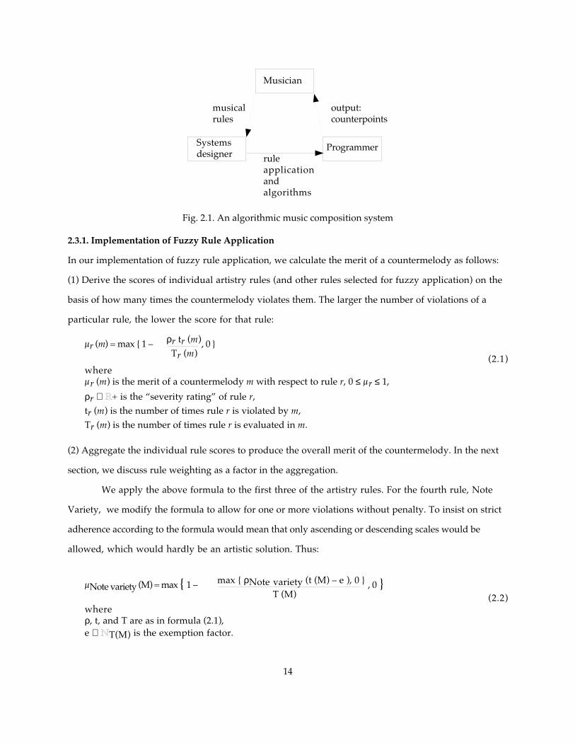
Musician

Systemsdesigner

Programmer

musicalrules

rule applicationandalgorithms

output:counterpoints

Fig. 2.1. An algorithmic music composition system

2.3.1. Implementation of Fuzzy Rule Application

In our implementation of fuzzy rule application, we calculate the merit of a countermelody as follows:

(1) Derive the scores of individual artistry rules (and other rules selected for fuzzy application) on the

basis of how many times the countermelody violates them. The larger the number of violations of a

particular rule, the lower the score for that rule:

µr (m) = max { 1 – , 0 }ρr tr (m)Tr (m) (2.1)

whereµr (m) is the merit of a countermelody m with respect to rule r, 0 ≤ µr ≤ 1,

ρr ∈ R+ is the “severity rating” of rule r, tr (m) is the number of times rule r is violated by m,Tr (m) is the number of times rule r is evaluated in m.

(2) Aggregate the individual rule scores to produce the overall merit of the countermelody. In the next

section, we discuss rule weighting as a factor in the aggregation.

We apply the above formula to the first three of the artistry rules. For the fourth rule, Note

Variety, we modify the formula to allow for one or more violations without penalty. To insist on strict

adherence according to the formula would mean that only ascending or descending scales would be

allowed, which would hardly be an artistic solution. Thus:

µNote variety (M) = max { 1 – , 0 } max { ρNote variety (t (M) – e ), 0 }T (M) (2.2)

whereρ, t, and T are as in formula (2.1),e ∈ NT(M) is the exemption factor.

14

Currently we have kept ρ = 1 a fixed quantity for all the four rules, and used e = 3. Thus, the score for

melody (b) in example 2.6 (<D, h, a, G, F, E, D>) under the Tonality Rule is derived as follows:

µTonality = max { 1 – 1/7, 0 } = 0.86. The score for melody (a) of example 2.5 (<D, E, D, E, D, C#, D>) is

µNote variety = max { 1 – max { ( 4 – 3 ), 0 } / 7, 0 } = 0.86. In this example, there were four violations:

three for the repetitions of the note “D”, and one for the repetition of the note “E”.

We have used the above evaluation method (with modifications for certain rules) to guide

heuristic searches for countermelodies. In the subsequent discussion, we refer to rules applied crisply as

crisp rules and those applied as described in section 2.3.1 as fuzzy rules. See chapter 6 for a description

of an exhaustive search algorithm (chapter 6, section 6.1), and for our use of the best-first branch-and-

bound and genetic algorithms (chapter 6, sections 6.1, 2); all three applications use the notion of crisp

and fuzzy rules for their respective evaluation functions.

2.3.2. Rule Weights

Humans compose music to a large extent by trial-and-error under the guidance of appropriate rules.

Algorithmic music composition systematizes this process, but remains dependent upon the same rules.

No rule set, however, can fully capture all the subtleties of a historical style, even for a simple model

like species counterpoint. Moreover, as complexity analysis will indicate (chapter 4), a program armed

with these rules can often produce a surfeit of countermelodies, albeit correct. A skilled composer has no

trouble eliminating from consideration a large number of these, and even discriminate among many

artistic possibilities. Clearly, the composer relies on more than just explicit rules in the decision-

making process.

Example 2.9. Given the following four competing countermelodies (CM 1–4) for cantus firmus CF, most musicians would prefer countermelody CM 1 over the other three, for all that CM 3 is the most “correct” if we include Lewin’s Rule in judging these countermelodies.

CM 4: a a a h a C# DCM 3: D E D E D C# DCM 2: a E F E D C# DCM 1: a a F E D C# DCF: D C# D G F E D �

To develop methods that more closely reflect expert preferences, we next consider the notion of

rule weights, whereby we can distinguish among the relative importance of each rule. Not all rules are

equal in importance, at least in the minds of composers and most listeners. Some are fundamental, and

these are best applied crisply, to enforce the notion that no melody should ever violate them; others

15

are fairly significant, but their violation by a melody is not always fatal; yet others represent

qualities that are nice to have but not absolutely essential. No masterpiece is perfect, but their very

imperfection reflects their human artistry. Assigning weightings to rules that are less than

fundamental allows us to reflect human artistry.

After assigning each of these rules a numerical weighting, the easiest way to calculate the

overall merit of a countermelody would be to find the weighted average of the evaluations of all these

rules. The formula for the overall merit of a countermelody m is thus:

∑wr n

r=1

∑ wr µr (m)

r=1

n

µ (m) =

(2.3)whereµ (m) is the overall merit of countermelody m,n is the total number of rules,wris the weighting of rule r, 1 ≤ r ≤ n, w ≥ 0,µr is the merit of m with respect to rule r, 1 ≤ r ≤ n.

We use rule weights to calculate a countermelody’s merit in a method to model human preferences

(chapter 5, section 5.1).

2.4. Summary

The challenge in species counterpoint composition is in having to comply with melody, harmony, and

counterpoint rules (“correctness” rules). These rules, unfortunately, while ensuring to some degree the

correctness of a counterpoint solution, fall far short of ensuring artistic results. Our introduction of

artistry rules, together with the concept of the fuzzy application of rules, addresses this difficulty.

We also considered the issue of rule redundancy and indispensability. We found that two rules

in particular, Lewin’s and the Dissonant Harmonic Intervals Rules, accounted for a significant number of

rejections of potential solutions.

16

CHAPTER 3. SPECIES COUNTERPOINT AND THE FINITE STATE MODEL

Applying fuzzy rules is only a first step in the process of musical composition. This overall

compositional process is quite computationally intensive, as we now show over this and the next

chapter. We shall formally define several problems based on species counterpoint. We then prove that

the more general among them belong to the NP-complete and other similarly complex categories,

whereas more restricted, but still musically useful, problems can be solved efficiently using simple

models like the finite state machine. In this chapter we discuss the restricted problems solvable on

simple models; in the next chapter we discuss the more general problems.

In confining our analysis to first species counterpoint, we have not lost generality. To encompass

the other species, we need not define entirely new problems, but simply alter the format of the cantus

firmus; to obtain second species (two notes in the added melody to one in the cantus firmus) or fourth

species (predominantly syncopated movement in the added part), we modify the given cantus firmus to

repeat every note; to obtain third species (four notes in the added melody to one in the cantus firmus),

we modify the cantus firmus to repeat every note thrice. For the fourth species, we specify the rules

accordingly to obtain the predominantly syncopated movement; for the fifth species, we repeat the

cantus firmus notes as many times as we wish to subdivide their beat.

Example 3.1. The following notations of counterpoints taken from Jeppesen (1931) show how to represent second and fourth species counterpoint by altering the format of the cantus firmus (compare the notation in example 1.1).

Second species, two parts:countermelody: a h c d e d f F G a b F a h c#(c#) dcantus firmus: D D a a G G F F E E D D F F E E D

(Jeppesen 1931, 117)Fourth species, two parts: countermelody: a a d d c c h h e e d e c c b a d d c# dcantus firmus: D D F F E E D D G G F F a a G G F F E E D

(Jeppesen 1931, 134) �

3.1. Restricted Problems Efficiently Solvable by the Finite State Model

The simplest problems are those dependent upon a history of a fixed number of notes in a single added

part. We have defined one such version (HM2PAL RESTRICTED) in a standard format, which we shall

use throughout this dissertation: we first describe the components of an instance of the problem, and

then ask a question about an instance that requires a yes/no answer. For the more general form of this

problem (HM2PAL), see chapter 4, section 4.1.1.

17

Problem 3.1. HM2PAL RESTRICTED INSTANCE:

A finite set S;c ∈ N;

a sequence CF ∈ Sc;H: (S x S)→{0, 1};M: (S x S)→{0, 1};a function R: Sn x Sn → {0, 1}, n ∈ N

where R is defined as follows:R (<cf1, cf2, … , cfc>, <m1, m2, … , mc >)

= 1 if H (cfi, mi) = 1, 1 ≤ i ≤ candM (mi, mi+1) = 1, 1 ≤ i ≤ c – 1

= 0 otherwise.QUESTION:

Is there a CP ∈ Sc such that R (CF, CP) = 1?

We shall show that this problem can be solved efficiently by using one of the simplest of

computational models: the finite state machine. The input string is the cantus firmus, and arrival at

the final state corresponds to a “yes” answer to this instance of the problem.

3.1.1. Non-Deterministic Finite State Machine to Solve HM2PAL RESTRICTED

From the rule specifications, we construct a non-deterministic finite state machine. The general method

is as follows (algorithm 3.1).

(1) Create a start state (labeled “s”). (2) Create a distinct state for each permissible harmonic interval. For ease of subsequent modifications, we label the state “cm/cf”, where “cm” is the note of the countermelody and “cf” that of the cantus firmus.(3) Create transitions between source and destination states, with labels denoting cantus firmus notes (corresponding to the “cf” term in the destination state), wherever cmsource to cmdestination is a permissible melodic interval. From the start state, create transitions corresponding to the first note of the cantus firmus. (4) Designate final states.

Algorithm 3.1. Building a non-deterministic finite state machine from rule specifications

Example 3.2. Consider the following concrete instance of HM2PAL RESTRICTED: Its gamut consists of the following notes: C#, D, E, F, G, a, and h. The only permissible harmonic intervals are major and minor thirds, perfect fourths and fifths, major and minor sixths, and unison only on D. The only permissible melodic intervals are seconds and thirds. We can even stipulate the following additional restrictions, not accommodated for in HM3PAL RESTRICTED’s instance specification: No parallel perfect fifths are ever allowed, the first harmonic interval must be either a unison or a perfect fifth with the cantus firmus, which will always begin on D, and the final interval must be a unison on D. We now build the non-deterministic finite state machine for this instance, according to algorithm 3.1.

18

In step (2) of algorithm 3.1, the two possible beginning harmonies are “D/D” and “a/D”. For this instance, it is necessary to distinguish these two states (that are used only for the initial note of the countermelody/cantus firmus) from two more states with similar intervals, but which indicate later notes of the counterpoint; this we have done so by labeling these latter states “D/D’” (final state) and “a/D’” respectively.

For step (3), there is a transition between state “a/D” to state “G/E” (labeled “E”), but there is no transition between state “a/D” to state “E/C#” because this would cause an inadmissible melodic interval of the fourth; neither is there a transition between state “a/D” to state “h/E” because this would cause parallel perfect fifths.

Using algorithm 3.1, we produce a finite state machine for the above instance to produce correct countermelodies (fig. 3.1). �

E/C# a/C# F/D G/E a/Fa/D’ h/D h/E h/G

D/D’

D/D a/D

S

D

DE

E

C#

ED

C#

C#E

F E

C#

EF

C#

D

FG

C# F DE

G

F E

Fig. 3.1. Non-deterministic finite state machine for an instance of HM2PAL RESTRICTED

Computational theory tells us that both non-deterministic and the corresponding deterministic

finite state machines are equally powerful. Furthermore, given a non-deterministic finite state

machine as above, there exists an algorithm to verify whether there is a correct countermelody for a

given cantus firmus without having to construct a deterministic version, and that algorithm is

19

polynomial in the number of states and in the length of the given cantus firmus. This is formalized in

theorem 3.1 (Lewis and Papadimitriou 1998, 107).

Theorem 3.1. If M = (Q, ∑, ∆, q0, F) is a non-deterministic finite state machine, then there is

an algorithm to test “w ∈ L (M)” in time O (|Q|2|w|).

We now implement this algorithm to test membership of a string (cantus firmus CF) in the

language of the non-deterministic finite state machine (M). Our implementation applies the dynamic

programming technique to compute sets of reachable states after having read a partial string

(algorithm 3.2, after Lewis and Papadimitriou 1998, 106).

Algorithm TestCFInput: M = (Q, ∑, ∆, q0, F), CF = <cf1, cf2, … , cfc>.Output: result ∈ {accept, reject}.1. S0 := {q0}2. for n from 1 to c

Sn := ∪ {q: p ∈ Sn–1, (p, cfn, q) ∈ ∆}3. if Sc ∩ F ≠ ∅

result := acceptelse

result := reject.

Algorithm 3.2. Testing acceptance of a cantus firmus (CF) by a non-deterministic finite state machine (M)

For a fixed gamut and fixed harmony and melody rules, we need construct a corresponding (non-

deterministic) machine only once at the outset. Having constructed the finite state machine, we can

store its specification for subsequent use.

Example 3.3. Given the finite state machine constructed in example 3.2, and the cantus firmus <D, E, D, C#, D>, the answer is “yes, there is/are countermelodies that satisfy/ies all the rules,” but given the cantus firmus <D, C#, E, D>, the answer is “no, there are not.” The set of states Sn processed by TestCF for <D, E, D, C#, D>, and for <D, C#, E, D>, and their respective paths, are shown in figure 3.2. �

For restricted music decision problems solvable by the finite state machine, the following

complexity analysis applies: If the length of the cantus firmus is fixed, or if the application of rules is

limited to a fixed lookback distance, the number of states of the finite state machine and the required

number of steps to solve an instance of the problem are both polynomially bounded, as shown below:

20

1) All cantus firmi (“CF”) of fixed length LEN with LEN –1 history:

Number of states of an Non-Deterministic FSM: O ( |S|LEN ).Number of steps to search: O ( |S|2LEN ).

2) All cantus firmi of any length with fixed length history k (k < |CF|):

Number of states of an Non-Deterministic FSM: O ( |S|k+1 ).Number of steps to search: O ( |S|2k+2 . |CF| ).

(a )

n cfn Sn Path

0 S0 = {s} s

1 D S1 = {a/D, D/D} a/D D/D

2 E S2 = {G/E} G/E

3 D S3 = {F/D, h/D, a/D’} F/D h/D a/D’

4 C# S4 = {E/C#, a/C#} E/C# a/C#

5 D S5 = {D/D’, F/D, h/D} D/D’ F/D h/D

Since D/D’ ∈ F, result = accept.

(b)

n cfn Sn Path

0 S0 = {s} s

1 D S1 = {D/D, a/D} D/D a/D

2 C# S2 = {E/C#} E/C#

3 E S3 = {G/E} G/E

4 D S4 = {F/D, a/D’, h/D} F/D a/D’ h/D

Since neither F/D, a/D’, nor h/D is a final state, result = reject.

Fig. 3.2. Processing of cantus firmi (a) <D, E, D, C#, D> and (b) <D, C#, E, D> by the non-deterministic finite state machine of figure 3.1

21

Although for every non-deterministic finite state machine, there is an equivalent deterministic

finite state machine, and one that can process a cantus firmus in strictly linear time, there is a vast

difference in the space requirements, as the number of states of the latter may be exponential (the

power set of the number of states of the non-deterministic machine corresponding approximately to the

number of acceptable harmonies, is exponentially larger). Also, the construction of the equivalent

minimal deterministic finite state machine is super-polynomial in time complexity unless P = NP, as

theorem 3.2 suggests (Lewis and Papadimitriou, 1998, 330, there expressed as a corollary).

Theorem 3.2. There is no algorithm polynomial in both input and output that, given a non-deterministic finite state machine, constructs an equivalent minimum-state deterministic finite state machine, unless P = NP.

The corresponding enumeration problem asks the question: “How many valid countermelodies

are there?” We define it as follows (HM2PAL RESTRICTED ENUM).

Problem 3.2. HM2PAL RESTRICTED ENUMINSTANCE:

A finite set S;c ∈ N;

a sequence CF ∈ Sc;H: (S x S)→{0, 1};M: (S x S)→{0, 1};a function R: Sn x Sn → {0, 1}, n ∈ N

where R is defined as follows:R (<cf1, cf2, … , cfc>, <m1, m2, … , mc >)

= 1 if H (cfi, mi) = 1, 1 ≤ i ≤ candM (mi, mi+1) = 1, 1 ≤ i ≤ c – 1

= 0 otherwise.QUESTION:

How many sequences CP ∈ Sc are there such that R (CF, CP) = 1?

Using the non-deterministic finite state machine, the number of valid counterpoints can be computed by

storing at each state arrived an integer value reflecting the number of partial paths leading to it,

which is the sum of all partial paths to the states in its predecessor list (algorithm 3.3).

Example 3.4. Running the finite state machine shown in figure 3.1, the answer in the problem instance with cantus firmus <D, E, D, C#, D> is “one,” because there is only one path leading to the goal state (corresponding to the transitions a/D–>G/E–>F/D–>E/C#–>D/D’); for cantus firmus <D, C#, E, D>, the answer is obviously “zero.” Figure 3.3 illustrates the additional information needed to solve the enumeration problem. In this instance, the single final state D/D’ shows only one partial path; had F/D been also a final state, the number of valid countermelodies would have been three. �

22

Algorithm EnumerateCMInput: M = (Q, ∑, ∆, q0, F), CF = <cf1, cf2, … , cfc>.Output: rnumCountermelodies.1. S0 := {q0}2. NumPathsTo (q0) := 13. for n from 1 to c

Sn := ∪ {q: p ∈ Sn–1 , (p, cfn, q) ∈ ∆}for each s ∈ Sn

NumPathsTo (s) := ∑p∈ Sn–1 NumPathsTo (p ∈ Sn–1 , (p, cfn, s) ∈ ∆)4. F’ := Sc ∩ F5. if F’ ≠ ∅

numCountermelodies := ∑f∈ F’ NumPathsTo (f)else

numCountermelodies := 0.

Algorithm 3.3. Solving the enumeration problem by a non-deterministic finite state machine (M)

n cfn Sn Path

0 S0 = {s} s

1 D S1 = {a/D, D/D} a/D(1) D/D(1)

2 E S2 = {G/E} G/E(1)

3 D S3 = {F/D, h/D, a/D’} F/D(1) h/D(1) a/D’(1)

4 C# S4 = {E/C#, a/C#} E/C#(1) a/C#(2)

5 D S5 = {D/D’, F/D, h/D} D/D’(1) F/D(3)h/D(2)

Fig. 3.3. Additional information stored to solve the enumeration problem (compare example 3.3). The notation, e.g., a/C#(2) indicates that there are two paths leading to the state a/C# reached after the transition labeled “C#”.

The number problem asks the question: “Are there at least K countermelodies?” (K HM2PAL

RESTRICTED).

Problem 3.3. K HM2PAL RESTRICTED INSTANCE:

A finite set S;c, K ∈ N;

a sequence CF ∈ Sc;

23

H: (S x S)→{0, 1};M: (S x S)→{0, 1};a function R: Sn x Sn → {0, 1}, n ∈ N

where R is defined as follows:R (<cf1, cf2, … , cfc>, <m1, m2, … , mc >)

= 1 if H (cfi, mi) = 1, 1 ≤ i ≤ candM (mi, mi+1) = 1, 1 ≤ i ≤ c – 1

= 0 otherwise.QUESTION:

Are there at least K sequences CP ∈ Sc such that R (CF, CPi) = 1, 1 ≤ i ≤ K?

The question can be answered by counting the number of distinct paths leading to the goal state.

Example 3.5. For cantus firmus <D, E, D, C#, D>, the answer is “yes” for K = 1, “no” for K > 1; for cantus firmus <D, C#, E, D>, the answer is “no” for any non-zero K. Using the same adaptation as for the enumeration problem, we can easily answer this question, by inspecting the sum of the number of partial paths to the final states in Sc. �

3.1.2. Non-Deterministic Finite State Transducer for Output Related to HM2PAL RESTRICTED

By means of a simple modification to the finite state machine as constructed above, we obtain a finite

state transducer, a machine that is capable of outputting a suitable countermelody to a given cantus

firmus. We can adopt either the Moore (Moore 1956) or the Mealy (Mealy 1955) machine, since both

models are equivalent. In the Moore machine, the states specify the output, whereas in the Mealy

machine, the transitions specify the output. Using our convention of naming the states as “cm/cf”, where

“cm” is a note of the countermelody and “cf” is a note of the cantus firmus, the Moore machine would

produce “cm” at each state, and the Mealy machine would produce at the transition the “cm” specified

in the destination state. For the Moore machine, the start state produces a null character.

We use this transducer to produce a valid countermelody to a cantus firmus, if one exists, by

storing additional information in the form of a list of predecessor states (represented as Preds,n in

algorithm 3.4 below). We then use this list to reconstruct a valid countermelody, after ascertaining its

existence by first running the transducer. The first part of the algorithm extends TestCF to produce the

predecessor states list and the (possibly empty) set of final states reached after processing the input

string (algorithm 3.4). For each state reached in the processing of the input string, the algorithm

TestCF2 produces its predecessor list, which is a state of sets reached prior to the current state. We use

24

these sets of states to reconstruct a valid countermelody by starting with a final state that also belongs

to the final set of states produced by TestCF2 (algorithm 3.5). Notice that this algorithm produces some

valid countermelody from possibly several valid ones. Which countermelody it produces depends on

non-deterministic choices of states from the set of final states F’ and from the predecessor states list.

Algorithm TestCF2Input: M = (Q, ∑, ∆, q0, F), CF = <cf1, cf2, … , cfc>.Output: result ∈ {accept, reject},

F’ ⊆ F,Pred: (Q x N)→2Q.

1. S0 := {q0}2. Predq0,0 := {} // start state has no predecessor3. for n from 1 to c

Sn := ∪ {q: p ∈ Sn–1 , (p, cfn, q) ∈ ∆}for each s ∈ Sn

Preds,n := ∪ {p ∈ Sn–1 , (p, cfn, s) ∈ ∆}4. F’ := Sc ∩ F5. if F’ ≠ ∅

result := acceptelse

result := reject.

Algorithm 3.4. Testing acceptance of a cantus firmus (CF) and outputting a state predecessor list (Pred) by a non-deterministic finite state machine (M)

Building the transducer, testing a cantus firmus, and deriving a valid countermelody still

requires only polynomial computing time. The time complexity is O (|CF||Q|2) = O (|CF||S|4).

Should we desire a strictly linear computing time, we need to convert this non-deterministic machine

into a deterministic one. In this case, as with the non-deterministic finite state machine (section 3.1.1),

the number of states in the deterministic model may again become exponential in the size of the gamut,

and the construction itself will again be super-polynomial, unless P = NP.

Example 3.6. Countermelodies produced by the finite state transducer for cantus firmi <D, C#, D, F, E, D, C#, D>, <D, E, D, C#, D>, and <D, F, E, D, C#, D> are shown below:

1.Countermelody: D E F a G F E D Cantus firmus: D C# D F E D C# D

2. Countermelody: a G F E DCantus firmus: D E D C# D

3.Countermelody: No countermelody possibleCantus firmus: D F E D C# D �

25

Algorithm ConstructCMInput: M = (Q, ∑, ∆, q0, F),

CF = <cf1, cf2, … , cfc>.Output: CM = <cm1, … , cmc>.Assumption: TestCF2 accepts CF. 1. TestCF2 (M, CF, result, F’, Pred)2. f := some s ∈ F’3. cmc := Out (M, f ∈ F’)4. p := f5. for n from c–1 to 1

p’ := some s ∈ Predp, n+1 cmn := Out (M, p’ ) p := p’.

Subprogram OutInput: M = (Q, ∑, ∆, q0, F),

q ∈ Q, q = <cm, cf>, cm, cf ∈ ∑. Output: cm.

Algorithm 3.5. Constructing a valid countermelody (CM) from output of an accepting non-deterministic finite state transducer (M)

With more information regarding the relative merits of the allowable intervals, both melodic

and harmonic, it would also be possible to solve the corresponding optimization problem, which asks

the question: “What is the best countermelody?” As it stands, the answer to all instances for which the

answer to the decision problem is “yes” is the set of all the possible countermelodies, because they are

all equally good.

The finite state transducer constructed for the instance specified in example 3.2 can be modified

to enforce two extra rules that are commonly observed in much of the music composed during the

sixteenth century and beyond: the Recovery Rule and the Leading-tone Rule (defined in appendix A as

part of the Diatonic Resolution Rule).

• Recovery Rule (A leap must be followed by a step in the opposite direction):

If noten of the countermelody is p and noten+1 of the countermelody is q and noten+2 of the countermelody is r

Then if ascending (p, q) is truethen descending (q, r) is true and interval size (q, r) is second

and if descending (p, q) is true then ascending (q, r) is true and interval size (q, r) is second.

26

• Leading-tone Rule (The leading tone (C#) must rise):

If noten of the countermelody is C# Then noten+1 of the countermelody is D.

Example 3.7. Consider the following four melodic fragments:

(a) (i) D b c ( i i ) D b a

(b)( i ) … C# A … (i i ) … C# D …

Melody (a) (i) violates the Recovery Rule because the ascending leap D–b is followed by further ascending motion; melody (a) (ii) is correct according to this rule: after the ascending leap, the melody falls (by a step) in the opposite direction. Melodies (b) (i) and (ii) both have a C#, which is the leading-tone in the dorian mode and has to rise stepwise to D, and not go anywhere else; thus, melody (b) (ii) is correct, but melody (b) (i) is not. Note that this definition of the Recovery Rule is the stronger form of the more common definition (for the latter definition, see appendix A; for a further illustration of this rule, see chapter 2, example 2.8). �

The modified finite state transducer for the above instance of HM2PAL RESTRICTED would

then require many more states to reflect direction and size of approach (fig. 3.4). The process is

otherwise straightforward, if somewhat tedious. Although much more complicated than the original

transducer, a correct countermelody can still be computed in polynomial time.

Example 3.8. Output of the modified finite state transducer (fig. 3.4) to cantus firmi <D, E, D, C#, D, F, E, D, C#, D, E, D, C#, D> and <D, C#, D, E, F, G, E, F, D, C#, D> are given below:

1. (2 possible solutions: countermelody 1 and 2):countermelody 1: a G F E F a G F E F G F E Dcountermelody 2: a G F E F a G h a F G F E Dcantus firmus: D E D C#D F E D C# D E D C# D

2. (2 attempted solutions):countermelody 1: D E F G a h G a h a ? (no continuation is possible)countermelody 2: D E F G a h G a F ? (no continuation is possible)cantus firmus: D C# D E F G E F D C# D

3.countermelody: D E F G a h G a F G F E Dcantus firmus: D C# D E F G E F D E D C#D �

27

S

D/D’ a/D’

E/C# 2b

G/E 2a

D

C# E

D/D

F/D 2b

D

E/C# 3a

a/C# 2b

F/D 2a

a/D 2b

h/D 3b

a/F 2b

h/G 3b

C#

D FG

C#

a/C# 3b

E/C# 2a

G/E 2b

a/F 3b

C#E

F

D

F/D 3a

h/D 2b

D

C# EF

E

a/C# 2a

a/F 2a

C#

F

h/E 2b

h/G 2b

D

E G

F

D

C#

DF

G

E

E

C#

G/E 3a

EF

DD

E G

C#

FEF

C#D

F

Fig. 3.4. Modified finite state machine to enforce two extra rules

3.1.3. Weighted Finite State Transducers to Solve the Optimization Problem

In the optimization problem (HM2PAL OPTIMIZATION), we would like to find the “best”

countermelody, according to a criterion based on weights given to various harmonies and melodic

progressions.

Problem 3.4. HM2PAL OPTIMIZATION INSTANCE:

A finite set S;c ∈ N;

a sequence CF ∈ Sc;H: (S x S)→{0, 1};M: (S x S)→{0, 1};ValH: (S x S)→N0;

ValM: (S x S)→N0;

a function R: Sn x Sn → {0, 1}, n ∈ N

28

where R is defined as follows:R (<cf1, cf2, … , cfc>, <m1, m2, … , mc >)

= 1 if H (cfi, mi) = 1, 1 ≤ i ≤ candM (mi, mi+1) = 1, 1 ≤ i ≤ c – 1

= 0 otherwise.QUESTION:

What is the optimal sequence CP ∈ Sc that satisfies R (CF, CP) = 1and produces α =

Σi=1

c( ValH (cfi, mi) + ValM (cfi, mi) ) ] ?max [

CP

We can extend the functionality, although not the language recognition power, of the finite state

transducer to compute such “optimal” countermelodies. We establish the optimization criterion by

assigning weights to each state and transition, corresponding to the weights of the harmonies and

melodic progressions specified in the optimization problem; the optimal countermelody, then, is that

countermelody accumulating the highest aggregate of these weight values in the processing of the

cantus firmus. An extension to the dynamic programming method of determining string acceptance by a

non-deterministic finite state transducer enables us to derive the optimal countermelody in polynomial

time. As with Floyd’s all-pairs shortest path algorithm (Floyd 1962), the method involves storing the

optimal partial score for partial strings attained in the set of states reachable at that point. This

exploits, as does Floyd’s algorithm, the principle of optimality, which states that all subinstances of

an optimal solution are also optimal. In the following algorithm (3.6), we assign weights to harmonies

(corresponding to states); a simple extension would enable us to assign weights to melodic movements as

well. We shall use the output of this algorithm to construct the optimal countermelody, hence the need

to output F’ ⊆ F and Pred. As with Floyd’s algorithm, we implement this algorithm with |Q| by |Q|

matrices, but this time with two such matrices. Since any state may be arrived at more than once

(unlike Floyd’s algorithm on graphs, note repetition is possible), we need to store two matrices, and

alternate them when calculating optimal partial paths.

Example 3.9. Figure 3.5 illustrates output of the finite state transducer (see figure 3.1) with cantus firmus <D, E, D, C#, D, C#, D>; suppose all harmonies have the weight of 1, except for the harmony F/D, which has a weight of 2. There are then three valid countermelodies: <a, G, F, E, F, E, D>, <a, G, F, a, F, E, D>, and <a, G, F, E, D, E, D>. Of these, the first two are optimal, both with a cumulative score of 9 (fig. 3.5). Note that at level n = 5, Pred (F/D)5 could be either {E/C#} or {a/C#};

29

we arbitrarily chose {E/C#}; had we chosen {a/C#} instead, we would have obtained <a, G, F, a, G, F, E> as an optimal countermelody. �

Algorithm OptimalScoreInput: M = (Q, ∑, ∆, q0, F),

CF = <cf1, cf2, … , cfc>.Output: result ∈ {accept, reject},

optimalScore,F’ ⊆ F,Pred: (Q x N)→2Q. AccumulatedScore: (Q x N)→N

// accumulated score of a state during construction of partial melody1. S0 := {q0}2. AccumulatedScore (q0, 0) := 03. Predq0,0 = {}4. for n from 1 to c

Sn := ∪ {q: p ∈ Sn–1 , (p, cfn, q) ∈ ∆}for each s ∈ Sn

maxP := p: AccumulatedScore (p, n–1) = max [AccumulatedScore (p’, n–1)] p’ ∈ Sn–1 , (p’, cfn, s) ∈ ∆

AccumulatedScore (s, n) := AccumulatedScore (maxP, n–1) + Val (M, s)Preds,n := {maxP}

5. F’ := Sc ∩ F6. if F’ ≠ ∅

result := acceptoptimalScore := max (AccumulatedScore (p’, c) )

p’ ∈ F’else

result := rejectoptimalScore := undefined.

Subprogram ValInput: M = (Q, ∑, ∆, q0, F),

q ∈ Q, q = <cm, cf, v>, v ∈ N.Output: v.

Algorithm 3.6. Outputting the score of the optimal countermelody to cantus firmus CF by a weighted non-deterministic finite state transducer M

The algorithm to construct the optimal countermelody is similar to ConstructCM (algorithm

3.5), except here Pred always yields a singleton set. Recall that in ConstructCM, we always chose one

state among possibly several at each predecessor level; here, we simply take the single element in each

predecessor set.

30

n cfn Sn Optimal predecessor states Optimal CP

0 {s} s

1 D {a/D, D/D} a/D(1) D/D(1) a

2 E {G/E} G/E(2) G

3 D {F/D, a/D’, h/D} F/D(4) a/D’(3) h/D(3) F

4 C# {E/C#, a/C#} E/C#(5) a/C#(5) E

5 D {D/D’, F/D, h/D} D/D’(6) F/D(7) h/D(6) F

6 C# {E/C#, a/C#} E/C#(8) a/C#(8) E

7 D {D/D’, F/D, h/D} D/D’(9) F/D(10) h/D(9) D

non-optimal predecessor stateoptimal predecessor stateoptimal predecessor state of notes of optimal countermelody

Fig. 3.5. Computing the optimal countermelody to cantus firmus <D, E, D, C#, D, C#, D>

We can also adapt algorithm 3.6 to output the m best countermelodies (algorithm 3.7, to solve

problem HM2PAL m OPTIMIZATION).

Problem 3.5. HM2PAL m OPTIMIZATION INSTANCE:

A finite set S; c, m ∈ N;

a sequence CF ∈ Sc;H: (S x S)→{0, 1};M: (S x S)→{0, 1};ValH: (S x S)→N0;

ValM: (S x S)→N0;

a function R: Sn x Sn → {0, 1}, n ∈ N where R is defined as follows:R (<cf1, cf2, … , cfc>, <m1, m2, … , mc >)

= 1 if H (cfi, mi) = 1, 1 ≤ i ≤ candM (mi, mi+1) = 1, 1 ≤ i ≤ c – 1

= 0 otherwise.

31

QUESTION: What are the m optimal sequences CPj ∈ Sc that satisfy R (CF, CPj) = 1, 1 ≤ j ≤ mand produce

Σi=1

c( ValH (cfi, mi) + ValM (cfi, mi) ) ] α1 = max [

CP

Σi=1

c( ValH (cfi, mi) + ValM (cfi, mi) ) ] α2 = max [

CP–CP1

…

Σi=1

c( ValH (cfi, mi) + ValM (cfi, mi) ) ] ?αm = max [

CP–CP1–…–CPm–1

Here we store information not only for the best partial countermelody, but for the m best partial

countermelodies. Using a max heap to compute the m best partially accumulated scores, the time

complexity of this algorithm is O (|CF||Q|(m|Q|log (m|Q|) + m log m) ) = O (|CF||Q|2 m (log m + log

|Q|) = O (|CF||S|4 m (log m + log |S|) ).

Example 3.10. Consider again the finite state transducer (fig. 3.1), with cantus firmus <D, E, D, C#, D, C#, D>, and assume again, as in example 3.9, all harmonies are equally weighted with the value of 1, except for F/D, which has the weight of 2. Storing accumulated scores enables us to derive the m = 2 best countermelodies <a, G, F, E, F, E, D> and <a, G, F, a, G, F, E> (fig. 3.6). �

3.2. Restricted Problems that Cannot Be Solved by the Finite State Model

A finite state machine/transducer can implement only those rules that govern a fixed number of notes.

With its fixed number of states (hence the adjective “finite”), this simple computational model cannot

implement rules that govern notes spanning the entire length of the countermelody, or in fact all rules

that govern a number of notes that is any non-constant function of the length of the countermelody. This

length is variable, since it depends on the cantus firmus, whose length in turn is not fixed. For such rules,

there does not seem to be available any less powerful model than the most general computing model

itself, the Turing machine. Furthermore, these rules actually preclude the possibility of a polynomial

solution (see PAL and related problems, defined in chapter 4). This may cause some surprise, since the

validation of a countermelody by any one rule is never more than a linear function of its length.

32

Algorithm mBestInput: M = (Q, ∑, ∆, q0, F), CF = <cf1, cf2, … , cfc>, m ∈ N,

Val: Q→N,.// value of a stateOutput: result ∈ {accept, reject},

optimalScores = <opt1, opt2, … , optm>, opti ∈ N, 1 ≤ i ≤ m, // best m optimal scores

finalStates = <fin1, fin2, … , finm>, fini ∈ Q, 1 ≤ i ≤ m, // final states of the m optimal countermelodies

predListq,i = <q1, q2, …>, q, qn ∈ Q, 1 ≤ i ≤ c. // predecessor states of state q at step i

AccumulatedScore: (Q x N x N)→N. // accumulated best m scores of a state 1. S1 := ∪ {q: (q0, cf1, q) ∈ ∆}

2. for each s ∈ S1 Insert q0 into predLists,1 AccumulatedScore (s, 1, 1) := Val (M, s)

3. for n from 2 to cSn := ∪ {q: p ∈ Sn–1 , (p, cfn, q) ∈ ∆}

for each s ∈ Sn predLists,n := <>

for each p ∈ Sn–1 , (p, cfn, s) ∈ ∆ Index (p) := 1

for i from 1 to m // find the m best among all predecessors to smaxAccumulatedScore := 0for each p ∈ Sn–1 , (p, cfn, s) ∈ ∆, Index (p) ≤ |predListp,n–1|

if AccumulatedScore (p, n-1, Index (p) ) > maxAccumulatedScore maxAccumulatedScore := AccumulatedScore (p, n-1, Index (p) ) Index (p) := Index (p) + 1maxPi := p

if maxPi is defined Insert maxPi at end of predLists,n AccumulatedScore (s, n, i) := maxAccumulatedScore + Val (M, s)

4. F’ := Sc ∩ F

5. if F’ ≠ ∅result := acceptfor i from 1 to m

for each p ∈ F Index (p) := 1

maxAccumulatedScore := 0for each p ∈ F’

if AccumulatedScore (p, c, Index (p) ) > maxAccumulatedScoremaxAccumulatedScore := AccumulatedScore (p, c, Index (p) ) optimalState := pIndex (p) := Index (p) + 1

if optimalState is definedopti := maxAccumulatedScorefini := optimalState

elseresult := rejectfinalStates := ∅ .

Subprogram ValInput: M = (Q, ∑, ∆, q0, F), q ∈ Q, q = <cm, cf, v>, v ∈ N.Output: v.

Algorithm 3.7. Outputting the m best countermelodies to cantus firmus CF by a weighted non-deterministic finite state transducer M

33

n cfn Sn Optimal predecessor states m = 2 best CP’s

0 {s} s

1 D {a/D, D/D} a/D(1) D/D(1) a a

2 E {G/E} G/E(2) G G

3 D {F/D, a/D’, h/D} F/D(4) a/D’(3) h/D(3) F F

4 C# {E/C#, a/C#} E/C#(5) a/C#(5, 4) E a

5 D {D/D’, F/D, h/D} D/D’(6) F/D(7, 7) h/D(6, 5) F F

6 C# {E/C#, a/C#} E/C#(8, 8) a/C#(8, 8) E E

7 D {D/D’, F/D, h/D} D/D’(9, 9) F/D(10, 10) h/D(9, 9) D D

non-optimal predecessor stateoptimal predecessor stateoptimal predecessor state of notes of optimal countermelody

Fig. 3.6. Computing m = 2 best countermelodies to the cantus firmus <D, E, D, C#, D, C#, D>

Two rules that encompass the entire length of the melody are Lewin’s Rule (Lewin 1983) and

the Stepwise Motion Rule:

• Lewin’s Rule: For every non-final note m of a melody, there should exist a note n between m and the final note fi of the melody such that the musical interval m–n is a descending step if m is higher than fi, and an ascending step if m is lower than fi.

• Stepwise Motion Rule: Stepwise motion must predominate in a melody.

From the computational point of view, the complexity of validation of a countermelody by

these two rules is O (|countermelody|).

Example 3.11. Consider the application of Lewin’s and the Stepwise Motion Rule to the following counterpoints (countermelodies 1–3 are alternative solutions to the cantus firmus):

countermelody 3: D b a G F E Dcountermelody 2: a b a G F E Dcountermelody 1: D a A C# D E Dcantus firmus: a D F E D C# D

34

Countermelody 1 has an interval of a fourth between a and E: according to Lewin’s Rule, this space must be filled up by G and F, as done by countermelodies 2 and 3, both of which do not violate the rule. Countermelody 1 also transgresses the Stepwise Motion Rule: of the six melodic intervals, three are leaps (D–a, a–A, A–C#), far too high a proportion. Countermelody 2 consists entirely of stepwise motion, and thus does not violate this rule, but runs afoul of the Note Variety Rule, should the latter be applied. Countermelody 3 has the best balance of leap and step (one leap and five steps). The aim of both Lewin’s Rule and the Stepwise Motion Rule is to maintain smoothness; a countermelody that violates one rule often violates the other, as here. �

3.3. Summary

The non-deterministic finite state machine solves the decision problem HM2PAL RESTRICTED; the

non-deterministic finite state transducer can additionally output countermelodies. Adjustments to this

model result in the solution to the corresponding enumeration and number problem. A weighted finite

state transducer can be used to output the optimal countermelody, and also the m best countermelodies.

These machine models also solve their respective problems efficiently. Table 3.1 shows the

results of time complexity analysis presented in this chapter.

Table 3.1. Complexity of various properties of and operations with finite state machines

Property, activity Complexity

1. Testing membership in a non-deterministic finite state automaton O (|Q|2|w|)2. Number of states of an NDFSM with fixed-length CF, |CF|–1 history O (|S||CF|)3. Number of states of an NDFSM with fixed-length history k < |CF| O (|S|k+1)4. Deriving a valid countermelody with a finite state transducer O (|CF||S|4)5. Deriving m best countermelodies with a finite state transducer O (|CF||S|4

m (log m + log |S|) )

Finite state machines can solve music composition problems that require the retention of a

history of no more than a fixed number of notes. When the cantus firmus length is variable, this model

is inadequate. When the computational complexity of rule validation is non-constant, the music

composition problem becomes intractable, as we show in the next chapter.

35

CHAPTER 4. INTRACTABLE PROBLEMS IN SPECIES COUNTERPOINT

The species counterpoint problem in general is computationally extremely complex. We have seen that

the addition of rules that govern notes spanning entire lengths of countermelodies causes the problem to

be unsolvable by finite state machines. Indeed, it may prevent the problem from being solvable

efficiently at all. In this chapter, we shall identify and define several variations of these problems.

The form of these definitions enables us to prove their membership in specific complexity categories by

linking them to known problems with similar complexity properties.

The most extensively researched of the complexity categories is that known as “NP-complete.”

We begin by discussing intractable music composition problems that belong to this category. We then

define intractable music problems that belong to related complexity categories. These are the

enumeration, number, and optimization problems, which we shall show to belong to the respective #P-

complete, “strong sense” NP-complete, and NP-equivalent complexity classes.

To prove the membership of these problems to the respective intractability classes, we use

reduction techniques, some first described by Garey and Johnson (1979). We shall then be in a position to

outline a hierarchy of proofs of NP-completeness and other complexity properties with respect to

reductions from previously known problems with similar complexity properties.

4.1. NP-Complete Music Problems

NP-complete problems are the most well-known among the intractable problems. They are called NP

(for “non-deterministic polynomial”) because for each of them, if a solution were proposed for a

particular instance, that solution could be verified in a length of time of no more than a polynomial

factor of the input length of the problem itself. They are called NP-complete because they are in some

sense the most complex of these non-deterministic polynomial problems: if the NP-complete problems

were somehow shown to be solvable in polynomial time, then all problems in NP are also solvable in

polynomial time.

Many problems in algorithmic music composition can be shown to be NP-complete, and in this

chapter we examine several such problems. We begin by defining the most general problem, which we

call PAL, then we derive two specialized versions, called HM3PAL and HM2PAL respectively. In

chapter 3, section 3.1, we defined a restricted form of HM2PAL for which we presented a polynomial

solution based on the finite state machine model.

36

We cast the three problems named above (PAL, HM3PAL, and HM2PAL) as decision problems,

viz., those problems with output of either “yes” or “no.” This allows us to incorporate the problems into

the context of NP-completeness theory, which is limited to decision problems. The general problem

that we call “PAL” is one that, given a gamut of notes, a cantus firmus constructed from notes of this

gamut, the number of parts to be added, and a set of rules providing the necessary and sufficient

conditions for a solution consisting of the previously specified number of added parts, asks the question

whether it is possible to create the specified number of added parts that satisfy the given rules.

The more restricted HM3PAL problem specializes the general problem to two added parts, and

to two musical rules only: one pertaining to a harmonic feature and the other to a melody feature. The

other specialized HM2PAL problem also specifies two rules, as for HM3PAL, but restricts the problem

to a single added part. Both these problems are prefixed with “HM-” to indicate that they are based

on two rule types: harmony and melody. We define each of these problems in the following section

(4.1.1).

4.1.1. Formal Definitions of PAL-Related Decision Problems

The definitions below (PAL, HM3PAL, HM2PAL, etc.) use the format as used in chapter 3, section 3.1.

Since these are decision problems, the question in each case requires a yes/no answer.

Problem 4.1. PAL INSTANCE:

A finite set S; c, p ∈ N;

a sequence CF ∈ Sc;a function R: Sn x (Sn)p → {0, 1}, n ∈ N, whose computation is bounded by a polynomial in n*p.

QUESTION: Is there a p-tuple of sequences CP ∈ (Sc)p such that R (CF, CP) = 1?

Problem 4.2. HM3PAL INSTANCE:

A finite set S; positive integers c, d, c > 1, 1 ≤ d < c; (d is used to indicate the desired extent of

melodic measurement between notes in the same part [see definition of R])a sequence CF ∈ Sc;a function H: S x S x S → {0, 1}; (signifying “allowable” harmonic intervals);a function M: S x S → {0, 1}; (signifying “allowable” melodic intervals);a function R: Sn x (Sn)2 → {0, 1}, n ∈ N

where R is defined as follows:R (<cf1, cf2, … , cfc>, <<m11, m12, … , m1c >, <m21, m22, … , m2c >>)

= 1

37

if H (cfi, m1i, m2i) = 1, 1 ≤ i ≤ candM (m1i, m1j) = 1, 1 ≤ i < j ≤ c, j – i ≤ dandM (m2i, m2j) = 1, 1 ≤ i < j ≤ c, j – i ≤ d

= 0 otherwise.QUESTION:

Is there a CP ∈ (Sc)2 such that R (CF, CP) = 1?

Problem 4.3. HM2PAL INSTANCE:

A finite set S; positive integers c, d, c > 1, 1 ≤ d < c; (d is used to indicate the desired extent of

melodic measurement between notes in the same part [see definition of R])a sequence CF ∈ Sc;a function H: S x S → {0, 1}; (signifying “allowable” harmonic intervals);a function M: S x S → {0, 1}; (signifying “allowable” melodic intervals);a function R: Sn x Sn → {0, 1}, n ∈ N

where R is defined as follows:R (<cf1, cf2, … , cfc>, <m1, m2, … , mc >)

= 1 if H (cfi, mi) = 1, 1 ≤ i ≤ candM (mi, mj) = 1, 1 ≤ i < j ≤ c, j – i ≤ d

= 0 otherwise.QUESTION:

Is there a CP ∈ Sc such that R (CF, CP) = 1?

An even more formal definition of these problems uses the concept of languages, and the notion of

acceptance or rejection by Turing machines. Thus, LPAL defines the language corresponding to PAL.

Problem 4.4. LPAL = {<S, CF, CP, R>: S is a finite set,CF is a sequence <cf1, cf2, … , cfc> over S,

R: Sn x (Sn)p → {0, 1}, n, p ∈ N, is a function whose computation is bounded by a polynomial in n*p,

andthere exists a CP’ for which R (CF, CP’) = 1}.

A Turing machine determines membership of a proposed instance; an NP problem is one in which a

succinct certificate exists with which a non-deterministic Turing machine can verify, in a number of

steps no greater than a polynomial factor of the input which encodes that instance, whether that input

belongs in the language. For ease of explanation, we adopt the less formal definitions presented here.

38

Example 4.1. An instance of PAL is the following:

S = {FF, GG, A, Bb, B, C, C#, D, E, F, G, a, b, h, c, c#, d, e, f, f#, g, aa}c = 10p = 1CF = <d, c, h, c, h, a, h, a, F#, G>R is effected by the melody, harmony, and counterpoint rules (see appendix A, section A.1).

The answer to this problem is “yes.” �

PAL and HM3PAL are NP-complete. We could prove this in the following order: first show

that HM3PAL is NP-complete by reduction from a known NP-complete problem called “Three-

Dimensional Matching” (abbreviated to “3DM,” proven NP-complete by Karp [1972]). Then we may use

this result to show that PAL is NP-complete. We may also use this result to show that HM2PAL is NP-

complete. This latter result is rather unusual, because of the better-known NP-complete

problems—3SAT, 3DM, and 3-MATROID INTERSECTION—their two-dimensional counterparts,

2SAT, 2DM, and 2-MATROID INTERSECTION, are all tractable.

The above decision problems used crisp rules. It is straightforward to create their fuzzy rule

counterparts. For example, FUZZY PAL DECISION is the fuzzy rule equivalent of PAL.

Problem 4.5. FUZZY PAL DECISION INSTANCE:

A finite set S; c, p ∈ N;α ∈ N0;

a sequence CF ∈ Sc;a set of functions (“crisp rules”) R = {ru1, ru2, … , rur}, rui: Sn x (Sn)p → {0, 1}, n ∈ N, 1 ≤ i ≤ r,

a set of functions (“fuzzy rules”) A = {a1, a2, … , aq}, ai: Sn x (Sn)p → N0,n*p, n ∈ N, 1 ≤ i ≤ qwhere the computation of each element of R and A is bounded polynomially in n*p.

QUESTION: Is there a CP ∈ (Sc)p such that rui (CF, CP) = 1, 1 ≤ i ≤ rand

Σi=1

qai (CF, CP) ≥ α?

Example 4.2. The fuzzy version of the instance of PAL in example 4.1 is:

S, c, p, CF, R as for example 4.1, A is effected by the four artistry rules (see appendix A, section A.1.4), α = 34.

The answer to this instance is “yes,” but “no” if α = 36. �

39

Naturally, several variants of these decision problems come to mind: they include one that asks

about possible solutions that are similar to a given solution, correct or otherwise (PAL MIN

CHANGES), and another that asks about complete solutions given a partial one (FUZZY PAL

EXTENSION DECISION). The PAL MIN CHANGES problem relates to problems of melodic similarity

and clustering; the FUZZY PAL EXTENSION DECISION problem relates to a practical application to

favor an expert’s choice among alternatives (see the “Jeppesen Experiment”, chapter 5, section 5.1).

Problem 4.6. PAL MIN CHANGESINSTANCE:

A finite set S; c, p ∈ N;

a sequence CF ∈ Sc;a p-tuple of sequences CP ∈ (Sc)p;a function R: Sn x (Sn)p → {0, 1}, n ∈ N, whose computation is bounded by a polynomial in n*p;

a function Dist: (Sn)p x (Sn)p → N0, n ∈ N, whose computation is bounded polynomially in n*p;

k ∈ N0.QUESTION:

Is there a p-tuple of sequences CP’ ∈ (Sc)psuch thatR (CF, CP’) = 1andDist (CP, CP’) ≤ k?

Problem 4.7. FUZZY PAL EXTENSION DECISION INSTANCE:

A finite set S; c, p ∈ N;α ∈ N0;

a sequence CF ∈ Sc;a set of functions (“crisp rules”) R = {ru1, ru2, … , rur}, rui: Sn x (Sn)p → {0, 1}, n ∈ N, 1 ≤ i ≤ r,

a set of functions (“fuzzy rules”) A = {a1, a2, … , aq}, ai: Sn x (Sn)p → N0,n*p, 1 ≤ i ≤ qwhere the computation of each element of R and A is bounded polynomially in n*p;

a p-tuple of sequences PM = <<mel11, mel12, … , mel1c>, <mel21, mel22, … , mel2c>, … ,<melp1, melp2, … , melpc>>, where each sequence in PM is over S ∪ {λ}.

QUESTION: Is there a p-tuple of sequences CP’ = <<mel’11, mel’12, … , mel’1c>, <mel’21, mel’22, … ,

mel’2c>, … , mel’p1, mel’p2, … , mel’pc>, where each sequence in CP’ is over S and melxy ≠ λ→melxy = mel’xy, 1 ≤ x ≤ p, 1 ≤ y ≤ c,

such thatrui (CF, CP’) = 1, 1 ≤ i ≤ r

40

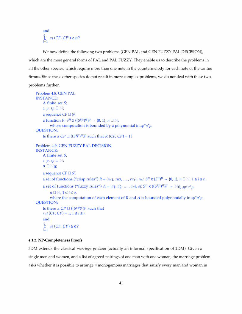
and

Σi=1

qai (CF, CP’) ≥ α?

We now define the following two problems (GEN PAL and GEN FUZZY PAL DECISION),

which are the most general forms of PAL and PAL FUZZY. They enable us to describe the problems in

all the other species, which require more than one note in the countermelody for each note of the cantus

firmus. Since these other species do not result in more complex problems, we do not deal with these two

problems further.

Problem 4.8. GEN PAL INSTANCE:

A finite set S; c, p, sp ∈ N;

a sequence CF ∈ Sc;a function R: Sn x ((Ssp)n)p → {0, 1}, n ∈ N,

whose computation is bounded by a polynomial in sp*n*p.QUESTION:

Is there a CP ∈ ((Ssp)n)p such that R (CF, CP) = 1?

Problem 4.9. GEN FUZZY PAL DECISION INSTANCE:

A finite set S; c, p, sp ∈ N;α ∈ N0;

a sequence CF ∈ Sc;a set of functions (“crisp rules”) R = {ru1, ru2, … , rur}, rui: Sn x (Sn)p → {0, 1}, n ∈ N, 1 ≤ i ≤ r,

a set of functions (“fuzzy rules”) A = {a1, a2, … , aq}, ai: Sn x ((Ssp)n)p → N0, sp*n*p,

n ∈ N, 1 ≤ i ≤ q,where the computation of each element of R and A is bounded polynomially in sp*n*p.

QUESTION: Is there a CP ∈ ((Ssp)c)p such that rui (CF, CP) = 1, 1 ≤ i ≤ rand

Σi=1

qai (CF, CP) ≥ α?

4.1.2. NP-Completeness Proofs

3DM extends the classical marriage problem (actually an informal specification of 2DM): Given n

single men and women, and a list of agreed pairings of one man with one woman, the marriage problem

asks whether it is possible to arrange n monogamous marriages that satisfy every man and woman in

41

the problem (see example 4.3 for instances of the marriage problem). With 3DM we may imagine three

different sexes (of n elements each) and a list of three-way matches. We then ask the question whether

it is possible to arrange n groupings that are “monogamous” and mutually acceptable. The marriage

problem can be solved in polynomial time, and is therefore tractable. 3DM, on the other hand, is NP-

complete.

Example 4.3. Two instances of the marriage problem are as follows:

(a )men = {a, b, c, d}women = {e, f, g, h}pairings = {<a, g>, <b, e>, <c, f>, <d, e>}

(b)men = {a, b, c, d}women = {e, f, g, h}pairings = {<a, g>, <b, e>, <b, h>, <c, f>, <d, e>}

The answer is “no” to the first instance, “yes” to the second (matching = {<a, g>, <b, h>, <c, f>, <d, e>}). �

Garey and Johnson (1978, 46) define 3DM as follows:

Problem 4.10. 3DM INSTANCE:

A set Ma ⊇ W x X x Y, where W, X, and Y are disjoint sets, each having q elements. QUESTION:

Does Ma contain a matching, that is, a subset Ma’ ⊇ Ma such that |Ma’| = q and no two elements of Ma’ are repeated in any coordinate?

To prove that HM3PAL is NP-complete, we first argue that it is an NP problem, i.e., it is

solvable by a non-deterministic polynomial algorithm. This is relatively easy to do, as is the case of

many NP-completeness proofs. We then show that 3DM polynomially reduces to HM3PAL, i.e., that

for any instance of 3DM, we can convert it to an instance of HM3PAL in polynomial time such that a

“yes” answer for that instance of 3DM results in a “yes” answer for the corresponding HM3PAL instance,

and such that a “no” answer results in a “no” answer for the corresponding HM3PAL instance.

Theorem 4.1. HM3PAL is NP-complete.

Proof: HM3PAL ∈ NP since a non-deterministic algorithm need only guess at a CP and evaluate R (CF, CP). The entire process can be accomplished in time polynomially bounded in c.

To show that HM3PAL is NP-hard, we transform an instance of 3DM to one of HM3PAL . Let W, X, and Y be disjoint sets having the same number q of elements, and Ma ⊇ W x X x Y be

an instance of 3DM. We shall construct an instance of HM3PAL: a finite set S, a sequence CF = <cf1, cf2, … , cfc> on S, and functions H and M

42

such that there is a sequence CP = <mel11, mel12, … , mel1c, mel21, mel22, … , mel2c> on S

such that R (CF, CP) = 1 if and only if Ma contains a matching Ma’ ⊇ Ma. Let i = W ∪ X ∪ Y. Let c = q. Let d = q – 1. (together with M’s definition, ensures no notes are repeated in each melody)Let CF = <cf1, cf2, … , cfc>, cfi ∈ W and cfi ≠ cfj whenever i ≠ j, 1 ≤ i ≤ c, 1 ≤ j ≤ c.

I.e., the elements of CF are a permutation of all the elements of W.Define H as follows:

H (z1, z2, z3) =1 if <z1, z2, z3> ∈ Ma

= 0 otherwise.Define M as follows:

M (z1, z2) = 1 if z1 ≠ z2= 0 otherwise.

It can be verified that this is a polynomial transformation, and that there is a CP such that R (CF, i) = 1 if and only if there is a matching Ma’ ⊇ Ma. �

The following example (4.4) illustrates a transformation from 3DM to HM3PAL.

Example 4.4. Consider the following two instances of 3DM:

(a )W = {a, b, c, d}X = {e, f, g, h}Y = {i, j, k, l}Ma = {<a, g, j>, <b, e, i>, <b, h, j>, <b, h, k>, <c, f, l>, <d, e, k>}

(b)W = {a, b, c, d}X = {e, f, g, h}Y = {i, j, k, l}Ma = {<a, g, j>, <b, e, i>, <b, h, i>, <b, h, k>, <c, f, l>, <d, e, k>}

The answers to the two instances are “no” and “yes,” respectively. The following is a matching for the second instance:

Ma’ = {<a, g, j>, <b, h, i>, <c, f, l>, <d, e, k>}

Transforming the second instance gives the following instance of HM3PAL:

S = {A, B, C#, D, E, F, G, a, b, c#, d, e}c = 4d = 3H = {<c#, E, A>, <c#, a, A>, <b, G, B>, <e, E, C#>, <c#, a, C#>, <d, F, D>}M = {<z1, z2>: z1 ≠ z2}CF = <A, B, C#, D> �

43

Once we have shown that HM3PAL is NP-complete, we can readily prove that the more

general problem PAL is NP-complete. We do so by reducing from the now “known” NP-complete problem

HM3PAL since the latter is a special case of the former.

Theorem 4.2. PAL is NP-complete.

Proof: Clearly, PAL is in NP. Restrict to HM3PAL by allowing only instances in which c > 1, p = 2, and R combines the functions H and M as specified. �

We next prove that HM2PAL is NP-complete, also by reducing from HM3PAL.

Theorem 4.3. HM2PAL is NP-complete.

Proof: HM2PAL ∈ NP since a non-deterministic algorithm need only guess at a CP and evaluate R (CF, CP) for 1 ≤ i ≤ c. The entire process can be accomplished in time polynomially bounded in c. To show that HM2PAL is NP-hard, we transform HM3PAL to HM2PAL as follows:

Let (S = S, c = c, d = d, CF = CF, H = H, M = M) be an instance of HM3PAL. We shall construct an instance (S’, c’, d’, CF’, H’, M’) of HM2PAL

such that there is a sequence CP’ = <mel1, mel2, … , melc> on S’ such that RHM2PAL (CF, CP) = 1 if and

only if there is a sequence CP = <mel11, mel12, … , mel1c, mel21, mel22, … , mel2c> on S such that RHM3PAL (CF, CP) = 1, where RHM2PAL and RHM3PAL refer to the R defined in HM2PAL and HM3PAL respectively. Let S’ = {a, b, ab, ba: a, b ∈ S}.Let c’ = c. Let d’ = d.Let CF’ = CF.Let H’ = {<a, bc, x>: <a, b, c, x> ∈ H}.Let M’ = {<ac, bd, z>: <a, b, x>, <c, d, y> ∈ M, z = 1 if x = y = 1, z = 0 otherwise}.

This is clearly a polynomial transformation of complexity O (|H| + |S|2 + |M|2). �

Example 4.5. Consider the following instance of HM3PAL :

S = {a, b, c, d}d = 1H = {<a, b, c, 1>, <b, c, d, 1>, <_,_,_, 0>} M = {<a, b, 1>, <b, c, 1>, <_, _, 0>} CF = <a, b, c>.

A transformation gives the following instance of HM2PAL:

S’ = {a, b, c, d, aa, bb, cc, dd, ab, ba, ac, ca, ad, da, bc, cb, bd, db, cd, dc}d = 1H’ = {<a, bc, 1>, <b, cd, 1>, <–,–, 0>}M’ = {<ab, bc, 1>, <ba, cb, 1>, <aa, bb, 1>, <bb, cc, 1>, <_,_, 0>}CF’ = <a, b, c>.

An example of a counterpoint in the above instance of HM3PAL is:

44

CM2: c a bCM1: b c aCF: a b c

whose equivalent in HM2PAL is:

CM’: bc ca abCF’: a b c

Both these counterpoints will not be accepted in both problems. In fact, for the above instances of HM3PAL and HM2PAL, no valid counterpoint is possible. Thus, the answer to the above instances of HM3PAL and HM2PAL is “no”. �

Example 4.6. Consider, however, the following instance of HM3PAL:

S = {a, b, c, d}d = 1H = {<a, b, c, 1>, <b, c, d, 1>, <_,_,_, 0>} M = {<a, b, 1>, <b, c, 1>, <c, d, 1>, <_, _, 0>} CF = <a, b>.

whose transformation into HM2PAL yields:

S’ = {a, b, c, d, aa, bb, cc, dd, ab, ba, ac, ca, ad, da, bc, cb, bd, db, cd, dc}d = 1H’ = {<a, bc, 1>, <b, cd, 1>, <–,–, 0>}M’ = {<ab, bc, 1>, <ba, cb, 1>, <aa, bb, 1>, <bb, cc, 1>,

<ac, bd, 1>, <ca, db, 1>, <bc, cd, 1>, <cb, dc, 1>, CF’ = <a, b>.

The answer to this instance is “yes”. There is one solution (for each of these instances of HM3PAL and HM2PAL):

HM3PAL:CM2: c dCM1: b cCF: a b

HM2PAL:CM’: bc cdCF’: a b �

We next prove that FUZZY PAL DECISION and PAL MIN CHANGES are NP-complete. To

show that the problems are in NP is trivial. We describe only the reductions necessary to complete the

proof.

Theorem 4.4. FUZZY PAL DECISION is NP-complete.

Proof: Restrict to PAL by allowing only instances having α = 0 and A = ∅ . �

Theorem 4.5. PAL MIN CHANGES is NP-complete.

45

Proof: Restrict to PAL by allowing only instances having Dist (CP, CP’) ∈ {0} and k = 0, with arbitrary CP. I.e., we ignore the distance component of the problem. �

We next show that FUZZY PAL EXTENSION DECISION is an NP problem. The reason we

included this problem is to provide a lemma to prove the theorem that the PAL-related optimization

problem—we shall call FUZZY PAL OPTIMIZATION—is NP-equivalent (theorem 4.11, section 4.2.3).

Lemma 4.1. FUZZY PAL EXTENSION DECISION is in NP.

Proof: A non-deterministic algorithm need only guess at a CP to complete PM, check that it extends PM in linear time, and verify it by applying the polynomially bounded rules. The entire process can be accomplished in time polynomially bounded in c*p*r*q. �

Note that FUZZY PAL DECISION is really a special case of FUZZY PAL EXTENSION

DECISION, with PM as the empty sequence; thus, FUZZY PAL EXTENSION DECISION can be easily

proven to be NP-complete as well. But its membership in NP is sufficient to prove NP-equivalence of

FUZZY PAL OPTIMIZATION (section 4.2.3).

4.1.3. An Alternative Proof of the NP-Completeness of PAL

Another NP-complete problem that can be polynomially transformed to PAL is the so-called

BOUNDED TILING problem. In this problem, we are asked whether it is possible to cover an s by s

square with various unit-length tiles given the tiling of the first row, and restrictions on which tiles

may be placed adjacent to each other both horizontally and vertically. It is defined as follows

(problem 4.11).

Problem 4.11. BOUNDED TILING INSTANCE:

A tiling system D = <D, H, V> whereD is a finite set of “tiles”;H: D x D → {0, 1};V: D x D → {0, 1};

s > 0;a function f0: {0, … , s – 1}→D.

QUESTION: Is there a function f: {0, 1, … , s – 1}x {0, 1, … , s – 1}→D such that

f (m, 0) = f0 (m), 0 ≤ m < s;<f (m, n), f (m+1, n)> ∈ H, 0 ≤ m < s – 1, 0 ≤ n < s;<f (m, n), f (m, n+1)> ∈ V, 0 ≤ m < s, 0 ≤ n < s – 1?

It is easy to see that D corresponds to S; H and V correspond to two rules in R (one governing melodic

progressions and the other governing harmonies); s = |CF| = p + 1; and f0 corresponds to CF.

46

Example 4.7. Consider the following instance of BOUNDED TILING:

D = {C#, D, E, F, G, a}H = {<C#, C#, 1>, <C#, D, 1>, <C#, E, 0>, <C#, F, 0>, <C#, G, 0>, <C#, a, 0>,

<D, C#, 1>, <D, D, 1>, <D, E, 1>, <D, F, 0>, <D, G, 1>, <D, a, 0>, <E, C#, 0>, <E, D, 1>, <E, E, 1>, <E, F, 1>, <E, G, 0>, <E, a, 1>, <F, C#, 0>, <F, D, 0>, <F, E, 1>, <F, F, 1>, <F, G, 1>, <F, a, 0>, <G, C#, 0>, <G, D, 0>, <G, E, 0>, <G, F, 1>, <G, G, 1>, <G, a, 1>, <a, C#, 0>, <a, D, 0>, <a, E, 0>, <a, F, 0>, <a, G, 1>, <a, a, 1>}

V = {<C#, C#, 0>, <C#, D, 0>, <C#, E, 1>, <C#, F, 0>, <C#, G, 0>, <C#, a, 0>,<D, C#, 0>, <D, D, 0>, <D, E, 0>, <D, F, 1>, <D, G, 0>, <D, a, 0>, <E, C#, 0>, <E, D, 0>, <E, E, 0>, <E, F, 0>, <E, G, 1>, <E, a, 1>, <F, C#, 0>, <F, D, 0>, <F, E, 0>, <F, F, 0>, <F, G, 0>, <F, a, 1>, <G, C#, 0>, <G, D, 1>, <G, E, 0>, <G, F, 0>, <G, G, 0>, <G, a, 0>, <a, C#, 0>, <a, D, 0>, <a, E, 1>, <a, F, 0>, <a, G, 0>, <a, a, 0>}

s = 3f0 = <D, C#, D>.

Transforming this gives the following instance of PAL:

S = {C#, D, E, F, G, a}c = 3p = 2CF = <D, C#, D>CP = <CM1, CM2>R (CF, CP) is such that only melodic movement of stepwise or unison motion is allowed, and only harmonies of consonant thirds and fourths are allowed.

The function R is described informally using musical terminology, but corresponds exactly to the combined effect of functions H and V of the BOUNDED TILING instance.

The answer to the BOUNDED TILING instance is “yes”: the following two tilings are valid:

(a ) (b)a a a a G aF E F F E FD C# D D C# D

These are also exactly the valid counterpoints for the corresponding PAL instance. �

In BOUNDED TILING, the size of the quadrant we are asked to tile is bounded by s; in the

unbounded version of BOUNDED TILING, we are asked to tile an infinite quadrant. It is interesting to

note that the unbounded version of this problem is undecidable.

The reader might also wish to consider the similarity of PAL with the following NP-complete

problem (FINITE STATE AUTOMATA INTERSECTION; Garey and Johnson 1979, 266; Kozen 1977),

which also involves the acceptance of strings by an external function, in this case a deterministic finite

state machine:

47

Problem 4.12. FINITE STATE AUTOMATA INTERSECTION INSTANCE:

A sequence A1, A2, … , An of deterministic finite state machines, all with the input alphabet ∑.QUESTION:

Is there a string x ∈ ∑* accepted by Ai, 1 ≤ i ≤ n?

In PAL, the function R (CF, CP) could be viewed as a deterministic Turing machine, and R (CF, CP) = 1

means that the machine accepts CP (with respect to CF) and R (CF, CP) = 0 means that the machine

rejects CF.

4.1.4. An Intractable Rule Redundancy Decision Problem

We return briefly to problems we introduced in chapter 2, section 2.1.1, viz., that of determining

redundancy and indispensability in rule sets. Here we discuss a more demanding version of these two

problems and prove that it is NP-complete. Recall that the simpler problems involved determining the

existence of a proper subset of the rules that did not duplicate the selectivity of any other rule in the

subset, and determining the existence of a set of rules that were uniquely responsible for the elimination

of some candidate countermelodies. We found there that the practical methods used did not always

yield optimal results: a great deal depended on the acceptance sets themselves. This would lead us to

suspect that the general problem might be intractable. We now define the generalized decision problem

(PAL RULE SUBSET) as that of determining the existence of a subset of specified size that succeeds in

eliminating the same countermelodies as would all the rules combined. First we define a related NP-

complete problem, VERTEX COVER (Garey and Johnson 1978, 46).

Problem 4.13. VERTEX COVER INSTANCE:

A graph G = (V, E) and a positive integer K ≤ |V|.QUESTION:

Is there a vertex cover of size K or less for G, i.e., a subset V’ ⊆ V such that |V’| ≤ K and, for each edge {u, v} ∈ E, at least one of u and v belongs to V’?

Our definition of PAL RULE SUBSET follows (problem 4.14).

Problem 4.14. PAL RULE SUBSET INSTANCE:

A cantus firmus set CFSet = {cf1, cf2, … , cfm};a rule set RSet = {r1, r2, … , rn};a collection of “Acceptance sets” Acceptr, c, 1 ≤ r ≤ n, 1 ≤ c ≤ m, which is the set of countermelodies for cfc ∈ CFSet that rule rr accepts;a positive integer K ≤ |RSet|.

QUESTION: Is there a subset RSet’ ⊆ RSet, |RSet’| ≤ K

48

such that∩ Acceptr, c

1≤r≤|RSet’|= ∩ Accepts, c

1≤s≤|RSet| , 1 ≤ c ≤ m ?

Theorem 4.6. PAL RULE SUBSET is NP-complete.

Proof: PAL RULE SUBSET is in NP, because given RSet’, checking the condition in the question can be accomplished in polynomial time. To prove PAL RULE SUBSET is NP-hard, restrict to VERTEX COVER. Note that for each Acceptr, c we have Rejectr, c = complement of Acceptr, c, where Rejectr, c is the set of countermelodies rejected by rule rr. Then, the intersection of all the acceptance sets = complement of the union of all the rejection sets (this follows from the definitions of acceptance and rejection sets made in chapter 2, section 2.1.1). Given an instance of VERTEX COVER, we create an instance of PAL RULE SUBSET as follows: let m = 1, let RSet = V, Rejectr, 1 = set of all edges incident on the corresponding vertex; the integer K is identical for both problems. �

Example 4.8. Consider the following instance of VERTEX COVER (fig. 4.1):

G = (V, E); V = {a, b, c, d}; E = { {a, c}, {a, d}, {b, c} }.

The transformation gives us the following instance of PAL RULE SUBSET:

m = 1; RSet = {r1, r2, r3, r4}; Reject1,1 = { ac, ad }; Reject2,1 = { bc }; Reject3,1 = { ac, bc };Reject4,1 = { ad }.

The answer for both problems is “yes” for K ≥ 2, “no” otherwise. There are three minimal vertex covers: {a, b}, {a, c}, are {c, d}; the three minimal rule sets are, of course, {r1, r2}, {r1, r3}, and {r3, r4} (fig. 4.1).

Observe that edges in G incident upon a particular vertex correspond to countermelodies rejected by the corresponding rule, while edges in G not incident upon a vertex correspond to countermelodies accepted by the corresponding rule, but rejected by some other rule/s. Also, all possible edges in G not actually in G correspond to countermelodies accepted by all the rules, or equivalently, the intersection of all the acceptance sets (fig. 4.2). �

a b

cd

a b

cd

a b

cd

a b

cd

(a) (b) (c) (d)

Fig. 4.1. Three distinct vertex covers ({a, b}, {a, c}, and {c, d}) for a graph G (represented in 4.1a); (b)–(d) illustrate the effect of the three vertex covers.

49

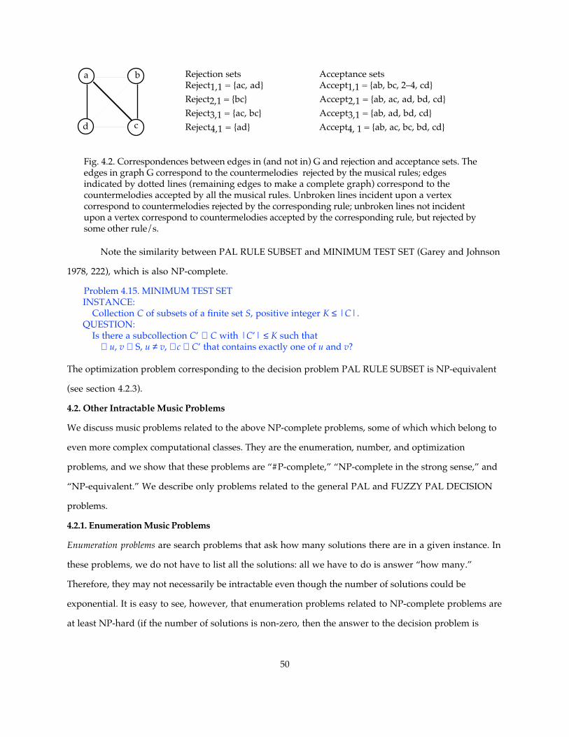
a b

cd

Rejection sets Acceptance setsReject1,1 = {ac, ad} Accept1,1 = {ab, bc, 2–4, cd}Reject2,1 = {bc} Accept2,1 = {ab, ac, ad, bd, cd}Reject3,1 = {ac, bc} Accept3,1 = {ab, ad, bd, cd}Reject4,1 = {ad} Accept4, 1 = {ab, ac, bc, bd, cd}

Fig. 4.2. Correspondences between edges in (and not in) G and rejection and acceptance sets. The edges in graph G correspond to the countermelodies rejected by the musical rules; edges indicated by dotted lines (remaining edges to make a complete graph) correspond to the countermelodies accepted by all the musical rules. Unbroken lines incident upon a vertex correspond to countermelodies rejected by the corresponding rule; unbroken lines not incident upon a vertex correspond to countermelodies accepted by the corresponding rule, but rejected by some other rule/s.

Note the similarity between PAL RULE SUBSET and MINIMUM TEST SET (Garey and Johnson

1978, 222), which is also NP-complete.

Problem 4.15. MINIMUM TEST SET INSTANCE:

Collection C of subsets of a finite set S, positive integer K ≤ |C|.QUESTION:

Is there a subcollection C’ ⊆ C with |C’| ≤ K such that ∀ u, v ∈ S, u ≠ v, ∃ c ∈ C’ that contains exactly one of u and v?

The optimization problem corresponding to the decision problem PAL RULE SUBSET is NP-equivalent

(see section 4.2.3).

4.2. Other Intractable Music Problems

We discuss music problems related to the above NP-complete problems, some of which which belong to

even more complex computational classes. They are the enumeration, number, and optimization

problems, and we show that these problems are “#P-complete,” “NP-complete in the strong sense,” and

“NP-equivalent.” We describe only problems related to the general PAL and FUZZY PAL DECISION

problems.

4.2.1. Enumeration Music Problems

Enumeration problems are search problems that ask how many solutions there are in a given instance. In

these problems, we do not have to list all the solutions: all we have to do is answer “how many.”

Therefore, they may not necessarily be intractable even though the number of solutions could be

exponential. It is easy to see, however, that enumeration problems related to NP-complete problems are

at least NP-hard (if the number of solutions is non-zero, then the answer to the decision problem is

50

“yes”, otherwise “no”). They may be intractable even if P = NP, so they belong to an interesting

complexity category. Valiant (1979, 1979b) introduced the complexity class #P, which contains

enumeration problems for which a non-deterministic polynomial algorithm exists that can guess

exactly the number of distinct solutions. The most difficult of the #P problems are the #P-complete

problems: they are those to which all other #P problems are Turing-reducible. To prove that a problem

is #P-complete, we may perform a special kind of Turing reduction known as parsimonious

transformation (first used by Simon [1975]): one in which the number of solutions of the transformed

instance is the same as that the original instance.

The enumeration music composition problems related to the PAL and FUZZY PAL DECISION

are PAL ENUM and FUZZY PAL ENUM. In the enumeration problems, we would like to know how

many solutions there are for a given cantus firmus. Some cantus firmi are more fruitful than others, and

if we could quickly determine their potential yield, we could adapt our search strategies accordingly; a

teacher of species counterpoint would know better the variety of answers to expect from students.

Problem 4.16. PAL ENUM INSTANCE:

As for PAL.QUESTION:

How many sequences CP are there such thatR (CF, i) = 1?

Problem 4.17. FUZZY PAL ENUM INSTANCE:

As for FUZZY PAL DECISION.QUESTION:

How many sequences CP are there such thatrui (CF, CP) = 1, 1 ≤ i ≤ rand

Σi=1

qai (CF, CP) ≥ α?

Example 4.9. Consider the following instance of PAL ENUM (compare example 4.1):

S = {FF, GG, A, Bb, B, C, C#, D, E, F, G, a, b, h, c, c#, d, e, f, f#, g, aa}c = 10p = 1CF = <d, c, h, c, h, a, h, a, F#, G>R combines the effect of the melody, harmony, and counterpoint rules (see appendix A, section A.1).

The answer for this instance of PAL ENUM is “55” (for the output of these 55 countermelodies, see appendix E, section E.3.2). �

51

Example 4.10. The corresponding instance of FUZZY PAL ENUM is:

S = {FF, GG, A, Bb, B, C, C#, D, E, F, G, a, b, h, c, c#, d, e, f, f#, g, aa}c = 10p = 1CF = <d, c, h, c, h, a, h, a, F#, G>R combines the effect of the melody, harmony, and counterpoint rules (see appendix A, section A.1)α = 34.

The answer for this instance is “17”. �

Theorem 4.7. PAL ENUM is #P-complete.

To prove this we need to define the enumeration problem associated with 3DM (let us call it

3DM ENUM).

Problem 4.18. 3DM ENUMINSTANCE:

As for 3DM.QUESTION:

How many matchings does M contain?

Example 4.11. An instance of 3DM ENUM that corresponds to the second instance of 3DM in example 4.4 would have the answer “1”. �

Proof (theorem 4.7): 3DM ENUM is #P-complete (Garey and Johnson 1979, Moret 1997). The transformation from 3DM ENUM to the enumeration version of HM3PAL (call it HM3PAL ENUM) is parsimonious, since clearly only those matchings in 3DM ENUM correspond to acceptable solutions in HM3PAL ENUM, and vice versa. The NP-completeness proof of PAL was a “restriction” proof by reduction from HM3PAL; consequently the transformation from HM3PAL ENUM to PAL ENUM is (strictly) parsimonious. �

Example 4.12. Using the instance of HM3PAL transformed above from the second instance of 3DM of example 4.4, the corresponding HM3PAL ENUM instance would have the answer “1” as well. �

Theorem 4.8. FUZZY PAL ENUM is #P-complete.

Proof: Restrict to PAL ENUM by allowing only instances having α = 0 and A = ∅ . This is a strictly parsimonious transformation, as are all “restriction” proofs (Moret 1997). �

4.2.2. Number Music Problems

A number problem is one in which the description of an instance contains one or more numbers whose

magnitude cannot be bounded by any polynomial in the size of the instance, using what is commonly

agreed as a reasonable encoding scheme of the instance. By “reasonable” we include almost all encoding

schemes except the unary encoding scheme; the most common reasonable scheme is binary because of its

ideal use in computers. A dynamic programming approach applied to these problems would still be

52

inefficient, all appearances to the contrary. For example, the well-known dynamic programming

solution to the KNAPSACK problem has a time complexity of Θ (nW), where n is the number of items

that can be stolen and W is the maximum capacity of the knapsack. Although it may appear that the

dynamic programming solution has a polynomial complexity (and a very good linear one at that),

unfortunately W is a number, or magnitude, and using a reasonable encoding scheme for it would render

the complexity of the solution exponential, not polynomial. Such solutions that are polynomial with

respect to the magnitude of some aspect of the input, but not necessarily to the size, are referred to as

pseudo-polynomial.

The number music problems related to the problems we have already defined are NP-complete

in the strong sense (terminology introduced by Garey and Johnson [1978]). These are decision problems

that cannot be solved even by a pseudo-polynomial algorithm, unless P = NP. Note, however, that the

definition of strong-sense NP-completeness implies that all NP-complete problems that are not number

problems are also NP-complete in the strong sense. Thus, the NP-complete problems defined in section

4.1 are all also NP-complete in the strong sense.

The related number music problems are K PAL and K FUZZY PAL. As defined below, these

number problems are similar in usefulness to the enumeration problems. Solutions to these problems

enable us to predict the fruitfulness of various cantus firmi.

Problem 4.19. K PAL INSTANCE:

A finite set S; c, p, K ∈ N;

a sequence CF ∈ Sc;a function R: Sn x (Sn)p→{0, 1}, n ∈ N, whose computation is bounded by a polynomial in n*p.

QUESTION: Are there at least K p-tuple of sequences CP ∈ (Sc)psuch thatR (CF, CPi) = 1, 1 ≤ i ≤ K?

Problem 4.20. K FUZZY PAL INSTANCE:

A finite set S; c, p ∈ N; K ∈ N0;

α ∈ N0;

a sequence CF ∈ Sc;

53

a set of functions (“crisp rules”) R = {ru1, ru2, … , rur}, rui: Sn x (Sn)p→{0, 1}, n ∈ N, 1 ≤ i ≤ r,

a set of functions (“fuzzy rules”) A = {a1, a2, … , aq}, ai: Sn x (Sn)p→N0,n*p, n ∈ N, 1 ≤ i ≤ qwhere the computation of each element of R and A is bounded polynomially in n*p.

QUESTION: Are there at least K p-tuple of sequences CP∈ (Sc)p such thatrui (CF, CPj) = 1, 1 ≤ i ≤ r, 1 ≤ j ≤ Kand

Σi=1

qai (CF, CPj) ≥ α , 1 ≤ j ≤ K?

Example 4.13. The instance of K FUZZY PAL corresponding to the instance of FUZZY PAL DECISION of example 4.2 has the answer “yes” if K = 17, but “no” for K > 17. �

In the following proofs, we again only show the reductions.

Lemma 4.2. K PAL is NP-complete.

Proof: Restrict to PAL by allowing only instances having K = 1. �

Theorem 4.9. K PAL is NP-complete in the strong sense.

Proof: K PAL is a number problem, since Max [I] = K and there exists no polynomial pol such that K ≤ pol (Length [I] ) for all I ∈ DK-PAL, where Max [I] is the magnitude of the largest number in problem instance I and Length [I] is the number of symbols used to describe problem instance I using a reasonable encoding scheme (definition by Garey and Johnson [1979, 92]). By Lemma 4.1, K PAL is NP-complete, proved by using a polynomial transformation from PAL by restricting K PAL to the subproblem with K = 1. With this restriction, Max [I] ≤ Length [I], and the subproblem of K PAL made up of all those instances satisfying this inequality is itself NP-complete. It follows that K PAL is NP-complete in the strong sense. �

Theorem 4.10. K FUZZY PAL is NP-complete in the strong sense.

Proof: Restrict to K PAL by allowing only instances having α = 0 and A = ∅ . �

We show below a partial reduction tree (fig. 4.3), which includes the polynomial

transformations we used in our proofs of the NP-complete music problems. The root problem is SAT (the

first problem proven to be NP-complete [Cook 1971]), and our tree shows the branch containing 3SAT

(proved NP-complete by Cook [1971]) and leading to 3DM, which we used to prove the NP-completeness

of HM3PAL. An analogous tree could be constructed for the reductions used in the enumerated versions of

these problems.

54

PAL

FUZZY PAL DECISION

SAT

3SAT

3DM

HM3PAL

PAL MIN CHANGES K PAL

K FUZZY PALFUZZY PAL EXTENSION DECISION

Fig. 4.3. NP-completeness proof transformation hierarchy for PAL-related problems

4.2.3. Optimization Music Problems

An optimization (sometimes referred to as combinatorial optimization) problem is one in which we seek

a solution that satisfies either a maximal or minimal condition. For example, an optimization music

problem requires a countermelody that has the highest possible merit. The complexity category to

which related optimization music problems belong will be shown to be NP-equivalent: these problems

are defined to be both NP-hard and NP-easy. An NP-hard problem is one to which every NP problem is

Turing reducible (equivalently, to which any NP-complete problem is Turing reducible); an NP-easy

problem is one which is Turing reducible to any NP problem. The terms “NP-equivalent” and “NP-easy”

were introduced by Garey and Johnson (1979) to encompass problems that are as difficult and as easy as

the NP-complete problems, within a polynomial factor; NP-equivalent problems are not necessarily

NP-complete themselves, because they are not necessarily decision problems.

The optimization problems are the decision problems modified to contain both fuzzy and crisp

rules; this combination of fuzzy and crisp rules is the basis of algorithms to reflect human preferences.

Our subsequent discussions on creating “human-like” music rest upon the problem we call FUZZY PAL

OPTIMIZATION.

55

Problem 4.21. FUZZY PAL OPTIMIZATION INSTANCE:

A finite set S; c, p ∈ N;

a sequence CF ∈ Sc;a set of functions (“crisp rules”) R = {ru1, ru2, … , rur}, rui: Sn x (Sn)p → {0, 1}, n ∈ N, 1 ≤ i ≤ r,

a set of functions (“fuzzy rules”) A = {a1, a2, … , aq}, ai: Sn x (Sn)p → N0,n*p, n ∈ N, 1 ≤ i ≤ qwhere the computation of each element of R and A is bounded polynomially in n*p.

QUESTION: What is the optimal p-tuple of sequences CP ∈ (Sc)p that satisfies rui (CF, CP) = 1, 1 ≤ i ≤ rand produces M =

Σi=1

qai (CF, CP) ] ?max [

CP

Lemma 4.3. FUZZY PAL OPTIMIZATION is NP-hard.

Proof: The Turing reduction from FUZZY PAL DECISION to FUZZY PAL OPTIMIZATION is straightforward. The solution to the optimization problem tells us the maximum possible value of α (call it αopt) in the decision problem, and the answer to the decision problem depends on the actual value of α in a given instance (call it α’): “yes” if α’ ≤ αopt, “no” otherwise. �

Lemma 4.4. FUZZY PAL OPTIMIZATION is NP-easy.

Proof: We present a constructive proof by showing a Turing reduction to FUZZY PAL EXTENSION DECISION. We use the solution to FUZZY PAL EXTENSION DECISION as an oracle to compute the optimal score M and then to derive the optimal sequence CP. To begin, notice that M ranges from 0 to c*p*r, and can be discovered for any instance of the problem with a polynomial number of calls to the FUZZY PAL EXTENSION DECISION oracle, using binary search: we start the search by querying the oracle for α = c*p*r/2 , and proceed by successively modifying α according to the oracle’s answers, always giving PM as the empty sequence. The complexity of deriving the optimal score in this way is no more than a polynomial in log (c*p*r) = (log c + log p + log r), since FUZZY PAL EXTENSION DECISION is in NP; let this optimal score be opt. If opt = 0, we are done, for any CP will do; otherwise, continue as follows: Build CP by querying the oracle, from now on always giving α = opt. We derive CP by building upon PM, each time querying the oracle for the validity of our choice of an element from S. The maximum number of queries is c*p*|S|; thus, the complexity of deriving CP is no more than a polynomial in c*p*|S|. The entire procedure queries the oracle a polynomial number of times, and therefore the entire reduction from FUZZY PAL OPTIMIZATION to FUZZY PAL EXTENSION DECISION runs in polynomial time. By definition, then, FUZZY PAL OPTIMIZATION is NP-easy. �

We now present the algorithm that is used in the above constructive proof of this theorem and

call it PALOptimization; it calls two subfunctions, FindOptimalCountermelodyGrade and

FindOptimalCountermelody. Both these subfunctions rely on an oracle, which is the putative solution

for the decision problem FUZZY PAL EXTENSION DECISION.

56

Algorithm PALOptimizationInput: S, CF, c, p, R, A.Output: optimalCountermelody.1. α := FindOptimalCountermelodyGrade (S, CF, c, p, R, A)2. optimalCountermelody := FindOptimalCountermelody (S, CF, c, p, R, A, α).

Subprogram FindOptimalCountermelodyGradeInput: S, CF, c, p, R, A.Output: α.1. for i from 1 to p

for j from 1 to cCP [i][j] := λ

2. low := 03. high := c*p*|S|4. while low ≤ high

mid := l (low + high)/2 m if ORACLE (S, CF, R, A, CP, mid) = “yes”

low := mid + 1else

high := mid - 1 5. α := high.

Subprogram FindOptimalCountermelodyInput: S, CF, c, p, R, A, α.Output: optimalCountermelody. 1. for i from 1 to p

for j from 1 to coptimalCountermelody [i][j] := empty

2. for i from 1 to pfor j from 1 to c

for each s ∈ SoptimalCountermelody [i][j] := sif ORACLE (S, CF, R, A, optimalCountermelody, α) = “yes”

break.

Algorithm 4.1. Solving FUZZY PAL OPTIMIZATION using the solution to FUZZY PAL EXTENSION DECISION

Example 4.14. Consider the following instance of FUZZY PAL OPTIMIZATION:

S= {C, C#, D, E, F}c = 4, p = 1, r = number of “crisp rules” (see appendix A, sections A.1.1–3), q = 3 CF = <D, E, C#, D>R is equivalent to the set of “crisp” rules (see appendix A, sections A.1.1–3)A is equivalent to the set consisting of the Tonality, Final in Leaps of Fourths and Fifths, and False Relations artistry rules (see appendix A, section A.1.4).

As outlined in the above proof, querying the FUZZY PAL EXTENSION DECISION oracle occurs in two stages:

57

Stage 1 (finding α):

QUESTION ANSWER

Is there a p-tuple of sequences CP’ = <<mel’11, mel’12, … , mel’1c>, <mel’21, mel’22, … ,mel’2c>, … , mel’p1, mel’p2, … , mel’pc>, where each sequence in CP’ is over S and melxy ≠ λ→melxy = mel’xy, 1 ≤ x ≤ p, 1 ≤ y ≤ c,

such thatrui (CF, CP’) = 1, 1 ≤ i ≤ rand

Σi=1

qai (CF, CP’) ≥ α?

Note: 0 ≤ α ≤ 12.

α = 6 yes9 yes11 yes12 no

CONCLUSION: α = 11.

Stage 2 (finding CP):

QUESTION ANSWER

Is there a p-tuple of sequences CP’ = <<mel’11, mel’12, … , mel’1c>, <mel’21, mel’22, … ,mel’2c>, … , mel’p1, mel’p2, … , mel’pc>, where each sequence in CP’ is over S and melxy ≠ λ→melxy = mel’xy, 1 ≤ x ≤ p, 1 ≤ y ≤ c,

such thatrui (CF, CP’) = 1, 1 ≤ i ≤ rand

Σi=1

qai (CF, CP’) ≥ 11?

PM = <C, λ, λ, λ> no<C#, λ, λ, λ> no<D, λ, λ, λ> yes<D, C, λ, λ> yes<D, C, C, λ> no<D, C, C#, λ> no<D, C, D, λ> no<D, C, E, λ> yes<D, C, E, C> no<D, C, E, C#> no<D, C, E, D> yes

CONCLUSION: The optimal CP is <D, C, E, D>. �

58

Theorem 4.11. FUZZY PAL OPTIMIZATION is NP-equivalent.

Proof: Since FUZZY PAL OPTIMIZATION is both NP-hard and NP-easy, by definition it is NP-equivalent. �

Finally, we consider the optimization problem related to the decision problem PAL RULE

SUBSET. Recall that in this problem we wanted to know if there was a rule subset of a given size that

eliminated the same countermelodies to a given cantus firmus as that by the entire rule set. In the

optimization version of this problem, we wish to know the smallest such subset that would eliminate

the same countermelodies. We now define PAL RULE SUBSET and prove that it is NP-equivalent.

Problem 4.22. PAL MINIMAL RULE SUBSETINSTANCE:

A cantus firmus set CFSet = {cf1, cf2, … , cfm};a rule set RSet = {r1, r2, … , rn};a collection of “Acceptance sets” Acceptr, c, 1 ≤ r ≤ n, 1 ≤ c ≤ m,

which is the set of countermelodies for cfc ∈ CFSet that rule rr accepts. QUESTION:

What is the minimal subset RSet’ ⊆ RSetsuch that

∩ Acceptr, c 1≤r≤|RSet’|

= ∩ Accepts, c1≤s≤|RSet| , 1 ≤ c ≤ m ?

Lemma 4.5. PAL MINIMAL RULE SUBSET is NP-hard.

Proof: Use a Turing reduction from PAL RULE SUBSET to PAL MINIMAL RULE SUBSET. �

Lemma 4.6. PAL MINIMAL RULE SUBSET is NP-easy.

Proof: We use the solution to the decision problem PAL RULE SUBSET as an oracle first to find the size of the minimal subset, and then to build this minimal subset, using a technique similar to that used in the NP-easiness proof of FUZZY PAL OPTIMIZATION. The first part of the proof requires no more than log2 |RSet| calls to the oracle. Suppose the size of the minimal rule set was found to be K’. We then proceed to build this minimal rule set, starting with the empty set. To determine which rules belong in this minimal rule set, we try adding each rule in turn to the minimal rule set. For each candidate rule considered for inclusion, we create modified acceptance sets of the rules that have not yet been added to the minimal rule set by removing those countermelodies implicitly rejected by the candidate rule and by rules that have already been determined to belong to the minimal rule subset. We present to the oracle the modified rule set which consists of RSet less the candidate rule and rules that have been determined to belong to the minimal rule set, the modified acceptance sets of rules not in the minimal rule set, and as the integer K the value of K’ (found in the first part of the proof) less the current size of the minimal rule set, and less one. If the oracle answers “yes”, we accept the candidate rule for inclusion into the minimal rule subset, otherwise we reject it. We proceed thus until the integer K becomes 0, in which case we cease asking the oracle (since the problem is not defined for K = 0), and instead select the final rule to be added to the minimal rule set by observing which one results in the remaining modified acceptance sets all becoming equal to the intersection of the original acceptance sets. In building the minimal rule subset in this way, the maximum number of calls to the oracle is |RSet|. �

59

We now present the algorithm that is used in the above constructive proof of this theorem,

which solves the optimization problem along similar lines as did the algorithm to solve FUZZY PAL

OPTIMIZATION. We call this present algorithm PALMinSubset, which calls two subfunctions,

FindMinSubsetSize and FindMinSubset. Both these subfunctions rely on an oracle, which is the

putative solution for the decision problem PAL RULE SUBSET.

Algorithm PALMinSubsetInput: CFSet, RSet, Acceptr,c, 1 ≤ r ≤ |RSet|, 1 ≤ c ≤ |CFSet|.Output: RSet’.1. K := FindMinSubsetSize (CFSet, RSet, Accept)2. RSet’ := FindMinSubset (CFSet, RSet, Accept, K).

Subprogram FindMinSubsetSizeInput: CFSet, RSet, Acceptr,c, 1 ≤ r ≤ |RSet|, 1 ≤ c ≤ |CFSet|.Output: K.1. low := 12. high := |RSet|3. while low ≤ high

mid := j (low + high)/2 k if ORACLE (CFSet, RSet, Accept, mid) = “yes”

high := mid - 1else

low := mid + 14. K := low.

Subprogram FindMinSubsetInput: CFSet, RSet, Acceptr,c, 1 ≤ r ≤ |RSet|, 1 ≤ c ≤ |CFSet|, K.Output: RSet’.1. RSet’ := {}2. K’ := K - 13. for i from 1 to |RSet|

tempRSet := RSet’ ∪ {ri}for j from i to |RSet|

for k from i to |CFSet|Accept’j,k := Acceptj,k ∩ Acceptr,k , 1 ≤ r ≤ tempRSet

if K’ > 0if ORACLE (CFSet, RSet - tempRSet, Accept’, K’) = “yes”

K’ := K’ - 1RSet’ := tempRSet

else // K’ = 0

1≤s≤|RSet|if Accept’j,k = ∩ Accepts,k, 1 ≤ k ≤ |CFSet|

RSet’ := tempRSetbreak.

Algorithm 4.2. Solving PAL MINIMAL RULE SUBSET using the solution to PAL RULE SUBSET

60

Example 4.15. Consider the following instance of PAL MINIMAL RULE SUBSET:

A single element CFSet, m = 1, RSet = {a, b, c, d, e}, Acceptance sets as follows:

Rule Acceptance seta {1, 3, 4, 5, 6, 7, 8}b { 3, 4, 5, 6, 7 }c { 2, 3, 4, 5, 6, 7, 8}d { 3, 4, 5, 7, 8}e { 3, 4, 5, 6, 8}

Queries to the oracle occur in two stages:

Stage 1 (finding the size of the minimal subset);

QUESTION ANSWER

Is there a subset RSet’ ⊆ RSet, |RSet’| ≤ Ksuch that

∩ Acceptr, c 1≤r≤|RSet’|

= ∩ Accepts, c1≤s≤|RSet| , 1 ≤ c ≤ m ?

Note: The possible values of K are in [1, 5].

K’ = 3? yes

K’ = 2? no

CONCLUSION: K’ = 3.

Stage 2 (building the minimal subset of size 3):

QUESTIONIs there a subset RSet’ ⊆ RSet, |RSet’| ≤ 3such that

∩ Acceptr, c 1≤r≤|RSet’|

= ∩ Accepts, c1≤s≤|RSet| , 1 ≤ c ≤ m ?

given

RSet = {b’, c’, d’, e’} // (Add rule a to CURRENT MINIMAL SUBSET = {}?)Rule (Modified) Acceptance setb’ {3, 4, 5, 6, 7 }c’ {3, 4, 5, 6, 7, 8}d’ {3, 4, 5, 7, 8}e’ {3, 4, 5, 6, 8}K = 2

ANSWER: no

61

RSet = {a’, c’, d’, e’} // (Add rule b to CURRENT MINIMAL SUBSET = {}?)Rule (Modified) Acceptance seta ’ {3, 4, 5, 6, 7}c’ {3, 4, 5, 6, 7}d’ {3, 4, 5, 7}e’ {3, 4, 5, 6 }K = 2

ANSWER: yes

RSet = {a’, d’, e’} // (Add rule c to CURRENT MINIMAL SUBSET = {b}?)Rule (Modified) Acceptance seta ’ {3, 4, 5, 6, 7}d’ {3, 4, 5, 7}e’ {3, 4, 5, 6 }K = 1

ANSWER: no

RSet = {a’, c’, e’} // (Add rule d to CURRENT MINIMAL SUBSET = {d}?)Rule (Modified) Acceptance seta ’ {3, 4, 5, 7}c’ {3, 4, 5, 7}e’ {3, 4, 5 }K = 1

ANSWER: yes

(Add rule e to CURRENT MINIMAL SUBSET = {b, d}?)a ’ {3 4 5}c’ {3 4 5}

Accepts, c1≤s≤|RSet|

, 1 ≤ c ≤ ma’ = c’ = {3, 4, 5} =

Accept rule e

CONCLUSION: Minimal rule subset = {b, d, e}. �

Note that in the second stage in building the minimal rule subset, once a rule has been considered for

inclusion in the minimal rule set but rejected because of a negative reply from the oracle, that rule need

not ever again be considered. Thus, in the instance in example 4.15, rules “a” and “b”, having drawn

negative responses from the oracle when considered initially for inclusion into the current empty rule

subset, need not be considered in subsequent attempts. Eliminating from consideration such rules,

however, does not improve the efficiency of the procedure by any order of magnitude.

Theorem 4.12. PAL MINIMAL RULE SUBSET is NP-equivalent.

Proof: Since MINIMAL RULE SUBSET is both NP-hard and NP-easy (lemmata 4.5, 4.6), by definition it is NP-equivalent. �

62

4.3. Summary

Rules that govern notes spanning entire countermelodies render the counterpoint composition problem

intractable. Among intractable music composition problems, we identified and classified such problems

as decision, enumeration, number, and optimization problems. Initially proving NP-completeness of one

decision music composition problem, HM3PAL, by reduction from 3DM (and alternatively, from

BOUNDED TILING), we established a hierarchy of proofs that show all related compositional

problems to be intractable as well. Table 4.1 summarizes the complexity classes to which the music

problems discussed in this chapter belong:

Table 4.1. Complexity classes of PAL-related problems

Problem Type Complexity class

1. PAL Decision NP-complete2. HM2PAL Decision NP-complete3. HM3PAL Decision NP-complete4. FUZZY PAL DECISION Decision NP-complete5. PAL MIN CHANGES Decision NP-complete6. PAL ENUM Enumeration #P-complete7. FUZZY PAL ENUM Enumeration #P-complete8. K PAL Number Strong sense NP-complete9. K FUZZY PAL Number Strong sense NP-complete10. FUZZY PAL OPTIMIZATION Optimization NP-equivalent

The general problems dealing with rule redundancy and indispensability, PAL RULE SUBSET

and PAL MINIMAL RULE SUBSET, are also intractable. We proved this initially by reduction from

VERTEX COVER.

63

CHAPTER 5. MODELING HUMAN PREFERENCES IN MUSIC COMPOSITION

In the classic Turing imitation game, a computer program tries to fool a person that its discourse springs

from another human being. We now try to write a program that can fool a person that its music, too,

springs from the creative imagination of another human being. For this to happen, that music needs to

reflect human preferences. We present two methods that use fuzzy rules to model such preferences: in

the first method (the “Jeppesen Experiment”), we collect a set of melodies composed by an expert, and

determine the relative importance the expert placed upon the various rules used in the compositional

process by calculating their weights (for our use of rule weights, see chapter 2, section 2.3.2); in the

second method, we train an artificial neural network to predict how a particular listener might

evaluate test melodies. We shall then be able to imbue heuristic methods (described in chapter 6) with

the ability to make choices among alternatives that reflect what a human expert might possibly

select.

5.1. The Jeppesen Experiment

In this method, we infer rule preferences directly from examples of a human expert. We first collect

countermelodies composed by an expert in species counterpoint; then we generate alternative

countermelodies at various points of the original compositions, and apply the fuzzy evaluation of a

predetermined set of rules. We assign weights to these rules in such a way that they favor the choice

the expert actually made over the alternatives. The goal is to create a weighted rule set that reflects

the expert’s value system. An authority on this style of music who has written a considerable corpus is

the Danish musicologist Knud Jeppesen (1931).

We carried out an experiment according to the procedure described in algorithm 5.1.

1. Select fuzzy rules.2. Fuzzify any remaining crisp rules violated by Jeppesen’s solutions.3. valid weight vector := <1, 1, …>.4. valid data set := Jeppesen’s original solutions.5. num blanks := 1.6. do

Prepare (data set, num blanks)if Adjust (weight vector, data set) is successful

valid weight vector := weight vector valid data set := data set increment num blanks

while num blanks ≤ |CF| and Adjust was successful.7. output valid weight vector and valid data set.

Algorithm 5.1. Procedure for the Jeppesen Experiment

64

In the experiment, we wanted to find a fuzzy rule weight vector that would favor one of

Jeppesen’s solutions to the cantus firmus <D, F, E, D, G, F, a, G, F, E, D>. The four fuzzy rules we used

were the artistry rules, and for Jeppesen’s solution in this instance (<a, aa, g, f, e, d, c, h, d, c#, d>) there

was no need to fuzzify any crisp rule. The initial valid weight vector was therefore <1, 1, 1, 1> to

weight each of the four fuzzy rules equally. The initial valid data set comprised Jeppesen’s solution

and the cantus firmus (listing 5.1). Listing 5.2 shows the data set with a single blank (characterized in

algorithm 5.1 as the output by subroutine Prepare), where “*” indicates blanks, or the opportunity for

alternatives. With the initially equally weighted fuzzy rules, the countermelody <a, aa, g, f, e, d, *,

h, d, c#, d> yielded two alternatives (Jeppesen’s solution is the second among these) that tied for the

highest score (listing 5.3). By adjusting the weight of the NoteVariety Rule by doubling it (i.e., weight

vector = <1, 1, 1, 2>), Jeppesen’s solution became the best choice among all alternatives (shown in listing

5.4 is Jeppesen’s solution followed by the formerly tied-for-first, now relegated to second-best,

alternative). Since we were able to adjust the weights successfully with one blank, we proceeded to

create a new data set with two blanks. Listing 5.5 shows the data set with two blanks. For this data

set, no further weight adjustments were necessary to preserve Jeppesen’s solution as the best. In fact, the

same weight vector was valid for all subsequent data sets with three and more blanks. The final data

set comprised a single countermelody with eleven blanks (corresponding to the eleven notes of the cantus

firmus), which essentially served to ask for all possible solutions to the cantus firmus. For this final

data set, there were 76 solutions. With the weight vector thus calculated, Jeppesen’s solution still

prevailed (shown in listing 5.6 is Jeppesen’s solution, followed by four alternatives that tied for second

place).

The need to increase the weightage of the NoteVariety rule in this instance indicates to some

extent that, for this cantus firmus at least, Jeppesen laid greater emphasis on note variety than he did

on, say, “false relations.” See appendix E, section E.1 for output of the genetic algorithm (chapter 6,

section 6.2) based on rules weighted according to the outcome of this instance of the Jeppesen

experiment: the genetic algorithm succeeded in finding the optimal countermelody (Jeppesen’s) very

quickly.

Listing 5.1. Initial valid data set

a aa g f e d c h d c# d D F E D G F a G F E D

65

Listing 5.2. Data set with one blank

* aa g f e d c h d c# dD F E D G F a G F E Da * g f e d c h d c# dD F E D G F a G F E Da aa * f e d c h d c# dD F E D G F a G F E Da aa g * e d c h d c# dD F E D G F a G F E Da aa g f * d c h d c# dD F E D G F a G F E Da aa g f e * c h d c# dD F E D G F a G F E Da aa g f e d * h d c# dD F E D G F a G F E Da aa g f e d c * d c# dD F E D G F a G F E Da aa g f e d c h * c# dD F E D G F a G F E Da aa g f e d c h d * dD F E D G F a G F E Da aa g f e d c h d c# *D F E D G F a G F E D

Listing 5.3. Solutions for data set with one blank

Countermelody: a aa g f e d * h d c# dCantus firmus: D F E D G F a G F E DAlpha cut: 0.0

Rule ρ w Tonality 1.0 1.0 Final in Leaps of 4ths and 5ths 1.0 1.0 False Relations 1.0 1.0 Note Variety 1.0 1.0

*** 1. Countermelody: a aa g f e d e h d c# d Cantus firmus: D F E D G F a G F E D

Rule Violations µ Tonality 00000001000 0.909091Final in Leaps of 4ths and 5ths 00000000000 1.000000 False Relations 00000000000 1.000000Note Variety 00001100100 0.727273

----------Overall rating: 0.909091

*** 2. Countermelody: a aa g f e d c h d c# d Cantus firmus: D F E D G F a G F E D

Rule Violations µ Tonality 00000001000 0.909091 Final in Leaps of 4ths and 5ths 00000000000 1.000000 False Relations 00000010000 0.909091

66

(listing 5.3 continued)

Note Variety 00000100100 0.818182 ----------

Overall rating: 0.909091 Number of solutions: 2.

Listing 5.4. Solutions for data set with one blank, and adjusted rule weights

Countermelody: a aa g f e d * h d c# dCantus firmus: D F E D G F a G F E DAlpha cut: 0.0

Rule ρ w Tonality 1.0 1.0 Final in Leaps of 4ths and 5ths 1.0 1.0 False Relations 1.0 1.0 Note Variety 1.0 2.0

*** 1. Countermelody: a aa g f e d c h d c# d Cantus firmus: D F E D G F a G F E D

Rule Violations µ Tonality 00000001000 0.909091 Final in Leaps of 4ths and 5ths 00000000000 1.000000 False Relations 00000010000 0.909091 Note Variety 00000100100 0.818182

----------Overall rating: 0.890909

*** 2. Countermelody: a aa g f e d e h d c# d Cantus firmus: D F E D G F a G F E D

Rule Violations µ Tonality 00000001000 0.909091 Final in Leaps of 4ths and 5ths 00000000000 1.000000 False Relations 00000000000 1.000000 Note Variety 00001100100 0.727273

----------Overall rating: 0.872727

Number of solutions: 2.

Listing 5.5. Data set with two blanks

* * g f e d c h d c# dD F E D G F a G F E Da * * f e d c h d c# dD F E D G F a G F E Da aa * * e d c h d c# dD F E D G F a G F E Da aa g * * d c h d c# dD F E D G F a G F E Da aa g f * * c h d c# dD F E D G F a G F E Da aa g f e * * h d c# d

67

(listing 5.5 continued)

D F E D G F a G F E Da aa g f e d * * d c# dD F E D G F a G F E Da aa g f e d c * * c# dD F E D G F a G F E Da aa g f e d c h * * dD F E D G F a G F E Da aa g f e d c h d * * D F E D G F a G F E D

Listing 5.6. Solutions for data set with eleven blanks, and adjusted rule weights

Countermelody: * * * * * * * * * * *Cantus firmus: D F E D G F a G F E DAlpha cut: 0.0

Rule ρ w Tonality 1.0 1.0 Final in Leaps of 4ths and 5ths 1.0 1.0 False Relations 1.0 1.0 Note Variety 1.0 2.0

*** 1. Countermelody: a aa g f e d c h d c# d Cantus firmus: D F E D G F a G F E D

Rule Violations µ Tonality 00000001000 0.909091 Final in Leaps of 4ths and 5ths 00000000000 1.000000 False Relations 00000010000 0.909091 Note Variety 00000100100 0.818182

----------Overall rating: 0.890909

*** 2. Countermelody: a a G F E D A B D C# D Cantus firmus: D F E D G F a G F E D

Rule Violations µ Tonality 00000001000 0.909091 Final in Leaps of 4ths and 5ths 00000000000 1.000000 False Relations 00000000000 1.000000 Note Variety 10000100100 0.727273

----------Overall rating: 0.872727

*** 3. Countermelody: a D G F E D A B D C# D Cantus firmus: D F E D G F a G F E D

Rule Violations µ Tonality 00000001000 0.909091 Final in Leaps of 4ths and 5ths 00000000000 1.000000 False Relations 00000000000 1.000000 Note Variety 01000100100 0.727273

----------

68

(listing 5.6 continued)

Overall rating: 0.872727*** 4. Countermelody: a aa g f e f e h d c# d Cantus firmus: D F E D G F a G F E D

Rule Violations µ Tonality 00000001000 0.909091 Final in Leaps of 4ths and 5ths 00000000000 1.000000 False Relations 00000000000 1.000000 Note Variety 00011000100 0.727273

----------Overall rating: 0.872727

*** 5. Countermelody: a aa g f e d e h d c# d Cantus firmus: D F E D G F a G F E D

Rule Violations µ Tonality 00000001000 0.909091 Final in Leaps of 4ths and 5ths 00000000000 1.000000 False Relations 00000000000 1.000000 Note Variety 00001100100 0.727273

----------Overall rating: 0.872727

Number of solutions: 5.

Notice that in proceeding with an increasing number of blanks in our data set, we produce sets of

countermelodies that are successively supersets of those produced with fewer blanks. Unlike in the

above experiment, it may happen that no valid weight vector can be found that makes Jeppesen’s

solution the best among new alternatives occasioned by a larger number of blanks, in which case we will

have to be satisfied with a sub-optimal solution related to a data set with a smaller number of blanks

than we would like. The optimal solution for a single cantus firmus, as above, is to have a weight vector

that makes Jeppesen’s solution prevail among all alternatives (num blanks = cantus firmus length). The

ultimate optimal solution is a weight vector valid for all cantus firmi attempted by Jeppesen.

We implemented this experiment by using the best-first search algorithm (described in chapter

6, section 6.1; for the implementation of the “fill in the blanks” algorithm, see appendix D, section

D.2.3). In each iteration of stage (6) of our procedure, we might have used this algorithm to generate all

alternatives for all the instances with num blanks filled. The algorithm automatically outputs the

alternatives in non-increasing order of merit, and it was not necessary for it to generate all possibilities,

only alternatives that included Jeppesen’s choice for us to know where the latter stands in each

instance. In the above experiment, Jeppesen’s choice always appeared as the best countermelody (either

69

tied or alone), both before and after weight adjustment, and we needed only to ask the best-first

algorithm to produce the best countermelody. This was sufficient for us to ensure that Jeppesen’s choice

was indeed favored above all alternatives after a suitable rule weight adjustment. In a less fortuitous

instance, we might have to ask for the two, or three, etc., best countermelodies, and at the worst, for all

alternatives. In appendix B, we show all the alternatives that could be generated at each iteration of

stage (6) of our procedure.

5.1.1. Complexity Analysis of the Jeppesen Experiment

In general, adjusting the rule weights in order to make Jeppesen’s solutions rate higher than the

alternatives can be formalized as problems that can be shown to relate closely to various forms of the

INTEGER PROGRAMMING problem, which in turn have been shown to be NP-complete or NP-hard by

several authors (Karp [1972], Sahni [1974], Borosh and Treybig [1976], Kannan and Monma [1978],

Papadimitriou [1981]). The simplest problem we have identified is what we have named FAVOR

JEPPESEN 0-1. This corresponds to the problem of whether or not to include a particular rule into a set

of equally weighted rules.

Problem 5.1. FAVOR JEPPESEN 0-1 INSTANCE:

A collection of finite string sets JM = { {jepp1, m11, m12, … , m1m1 }, {jepp2, m21, m22, … , m2m2}, … , {jeppn, mn1, mn2, … , mnmn} },

jeppi, mi1, mi2, … ∈ String, 1 ≤ i ≤ n;

a set of rules R = {R1, R2, … , Rr}, Ri: String→Z, 1 ≤ i ≤ r.QUESTION:

Is there a function w: R→{0, 1} such that

∑ (w (R) R (jeppk) ) ≥ max { ∑ (w (R) R (m ) ) }, 1 ≤ k ≤|JM|, ∑ w (R) > 0 ?kmk

kmk R∈ RR∈ R R∈ R

Theorem 5.1. FAVOR JEPPESEN 0-1 is NP-complete.

The proof of the above theorem restricts the problem to an instance of KNAPSACK (proven NP-

complete by Karp [1972]).

Problem 5.2. KNAPSACK INSTANCE:

Finite set U, for each u ∈ U a size s (u) ∈ N and a value v (u) ∈ N,

and positive integers B and K.QUESTION:

Is there a subset U’ ⊂– U such that

70

∑ s (u) ≤ Bu ∈ U’and such that

u ∈ U’∑ v (u) ≥ K ?

Proof (theorem 5.1): FAVOR JEPPESEN 0-1 is clearly in NP, a “guess” can easily be verified in polynomial time. To show that it is NP-hard, restrict it to KNAPSACK by allowing only instances in which

JM = { {jepp1, m11}, {jepp2, m21} }; R = {R1, R2, … , R|U|, R|U|+1}; Ri (jepp1) = v (ui), and Ri (m11) = 0, 1 ≤ i ≤ |U|; R|U|+1 (jepp1) = 0, and R|U|+1 (m11) = K; Ri (jepp2) = 0, and ri (m21) = s (ui), 1 ≤ i ≤ |U|; R|U|+1 (jepp2) = B, and R|U|+1 (m21) = 0; �

In this reduction, JM consists of two pairs of melodies. R contains |U| + 1 rules: with respect to

the set containing jepp1, the evaluations of the first |U| rules correspond to v (ui), while the

evaluation of the last rule corresponds to K; with respect to the set containing jepp2, the evaluations of

the first |U| rules correspond to s (ui), while the evaluation of the last rule corresponds to B.

In the definition of FAVOR JEPPESEN 0-1, note that the range space of the rules (represented

as functions) differs from that in the definition of PAL and related problems. If desired, the range space

of all rules could be restricted to [0..maxi{|jeppi|}], and in the proof specify further that max [|jepp1|,

|jepp2|] = maxi [v (ui)]. This will not alter the complexity of FAVOR JEPPESEN 0-1.

A more general problem is the following, where the chosen rules are allowed to be unequally

weighted (FAVOR JEPPESEN INTEGER). The proof of lemma 5.1 transforms a version of INTEGER

PROGRAMMING, proved NP-hard by Sahni (1974).

Problem 5.3. FAVOR JEPPESEN INTEGER INSTANCE:

A collection of finite string sets JM = { {jepp1, m11, m12, … , m1m1 }, {jepp2, m21, m22, … , m2m2}, … , {jeppn, mn1, mn2, … , mnmn} },

jeppi, mi1, mi2, … ∈ String, 1 ≤ i ≤ n;

a set of rules R = {R1, R2, … , Rr}, Ri: String→Z, 1 ≤ i ≤ r.QUESTION:

Is there a function w: R→Z such that

∑ (w (R) R (jeppk) ) ≥ max { ∑ (w (R) R (m ) ) }, 1 ≤ k ≤|JM|, ∑ w (R) > 0 ?kmk

kmk R∈ RR∈ R R∈ R

71

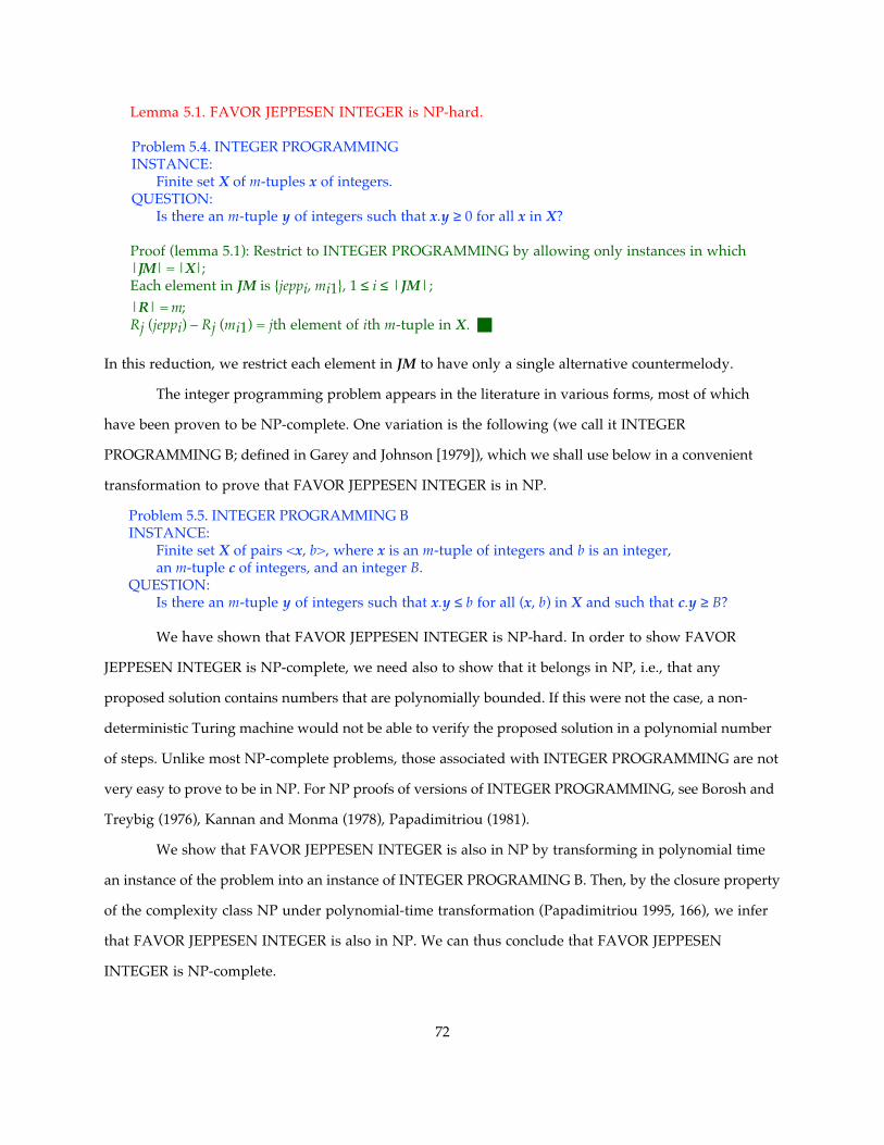
Lemma 5.1. FAVOR JEPPESEN INTEGER is NP-hard.

Problem 5.4. INTEGER PROGRAMMING INSTANCE:

Finite set X of m-tuples x of integers. QUESTION:

Is there an m-tuple y of integers such that x.y ≥ 0 for all x in X?

Proof (lemma 5.1): Restrict to INTEGER PROGRAMMING by allowing only instances in which|JM| = |X|;Each element in JM is {jeppi, mi1}, 1 ≤ i ≤ |JM|; |R| = m;Rj (jeppi) – Rj (mi1) = jth element of ith m-tuple in X. �

In this reduction, we restrict each element in JM to have only a single alternative countermelody.

The integer programming problem appears in the literature in various forms, most of which

have been proven to be NP-complete. One variation is the following (we call it INTEGER

PROGRAMMING B; defined in Garey and Johnson [1979]), which we shall use below in a convenient

transformation to prove that FAVOR JEPPESEN INTEGER is in NP.

Problem 5.5. INTEGER PROGRAMMING B INSTANCE:

Finite set X of pairs <x, b>, where x is an m-tuple of integers and b is an integer, an m-tuple c of integers, and an integer B.

QUESTION: Is there an m-tuple y of integers such that x.y ≤ b for all (x, b) in X and such that c.y ≥ B?

We have shown that FAVOR JEPPESEN INTEGER is NP-hard. In order to show FAVOR

JEPPESEN INTEGER is NP-complete, we need also to show that it belongs in NP, i.e., that any

proposed solution contains numbers that are polynomially bounded. If this were not the case, a non-

deterministic Turing machine would not be able to verify the proposed solution in a polynomial number

of steps. Unlike most NP-complete problems, those associated with INTEGER PROGRAMMING are not

very easy to prove to be in NP. For NP proofs of versions of INTEGER PROGRAMMING, see Borosh and

Treybig (1976), Kannan and Monma (1978), Papadimitriou (1981).

We show that FAVOR JEPPESEN INTEGER is also in NP by transforming in polynomial time

an instance of the problem into an instance of INTEGER PROGRAMING B. Then, by the closure property

of the complexity class NP under polynomial-time transformation (Papadimitriou 1995, 166), we infer

that FAVOR JEPPESEN INTEGER is also in NP. We can thus conclude that FAVOR JEPPESEN

INTEGER is NP-complete.

72

Theorem 5.2. FAVOR JEPPESEN INTEGER is NP-complete.

Proof: We first show a polynomial-time transformation of FAVOR JEPPESEN INTEGER to INTEGER PROGRAMMING B. Restrict to INTEGER PROGRAMMING B by allowing only instances in which m = |R|, x = 0 and b = 0 for all (x, b) in X; ci = ∑k Ri (jeppk) – ∑k maxkmk [Ri (mkmk)], for each ci in c, 1 ≤ i ≤ m; B = 0. Then, since INTEGER PROGRAMMING B is in NP, FAVOR JEPPESEN INTEGER is also in NP, by the closure property under polynomial-time transformation of NP. This, together with lemma 5.1, implies that FAVOR JEPPESEN INTEGER is NP-complete. �

In INTEGER PROGRAMMING, we require integer solutions, and this requirement makes the

problem NP-complete. On the other hand, LINEAR PROGRAMMING, wherein we accept any real

number solution, is a polynomial-time problem (Dobkin et al. [1976]), for which efficient algorithms

have been devised (see Dantzig [1963], Khachiyan [1979], and Karmarkar [1984]). Since FAVOR

JEPPESEN INTEGER is really INTEGER PROGRAMMING in disguise, if we accept any real number

solution, we could easily adapt algorithms for LINEAR PROGRAMMING to solve a tractable version

of FAVOR JEPPESEN INTEGER, which we shall call FAVOR JEPPESEN.

Problem 5.6. FAVOR JEPPESEN INSTANCE:

A collection of finite string sets JM = { {jepp1, m11, m12, … , m1m1 }, {jepp2, m21, m22, … , m2m2}, … , {jeppn, mn1, mn2, … , mnmn} },

jeppi, mi1, mi2, … ∈ String, 1 ≤ i ≤ n;

a set of rules R = {R1, R2, … , Rr}, Ri: String→Z, 1 ≤ i ≤ r.QUESTION:

Is there a function w: R→R such that

∑ (w (R) R (jeppk) ) ≥ max { ∑ (w (R) R (m ) ) }, 1 ≤ k ≤|JM|, ∑ w (R) > 0 ?kmk

kmk R∈ RR∈ R R∈ R

5.1.2. Related Jeppesen Problems

In this section, we consider related problems, and indicate why they are also intractable if we require

integer solutions. In the decision problems for the Jeppesen Experiment, we asked about the existence of

a function that would evaluate Jeppesen’s compositions favorably against all alternatives. What we

really would like to know in this experiment is, of course, what that function is, if it exists. Better yet,

if possible, we would like to know the function whose evaluation maximizes the scores of Jeppesen’s

compositions. To define the optimization problem that asks these questions, we proceed in the same

way that led to the optimization problem related to PAL. As a preliminary to the optimization

problem formulation, we define the following number problem (FAVOR JEPPESEN K).

73

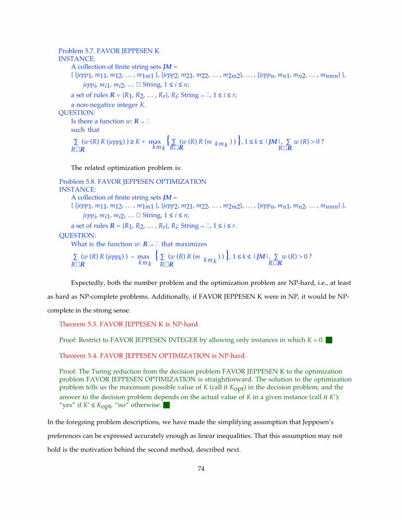
Problem 5.7. FAVOR JEPPESEN K INSTANCE:

A collection of finite string sets JM = { {jepp1, m11, m12, … , m1m1 }, {jepp2, m21, m22, … , m2m2}, … , {jeppn, mn1, mn2, … , mnmn} },

jeppi, mi1, mi2, … ∈ String, 1 ≤ i ≤ n;

a set of rules R = {R1, R2, … , Rr}, Ri: String→Z, 1 ≤ i ≤ r;a non-negative integer K.

QUESTION: Is there a function w: R→Z such that

R∈ R∑ (w (R) R (jeppk) ) ≥ K + max { ∑ (w (R) R (m ) ) }, 1 ≤ k ≤ |JM|, ∑ w (R) > 0 ?

kmkkmk

R∈ R R∈ R

The related optimization problem is:

Problem 5.8. FAVOR JEPPESEN OPTIMIZATION INSTANCE:

A collection of finite string sets JM = { {jepp1, m11, m12, … , m1m1 }, {jepp2, m21, m22, … , m2m2}, … , {jeppn, mn1, mn2, … , mnmn} },

jeppi, mi1, mi2, … ∈ String, 1 ≤ i ≤ n;

a set of rules R = {R1, R2, … , Rr}, Ri: String→Z, 1 ≤ i ≤ r.QUESTION:

What is the function w: R→Z that maximizes

R∈ R∑ (w (R) R (jeppk) ) – max { ∑ (w (R) R (m ) ) }, 1 ≤ k ≤ |JM|, ∑ w (R) > 0 ?

kmkkmkR∈ R R∈ R

Expectedly, both the number problem and the optimization problem are NP-hard, i.e., at least

as hard as NP-complete problems. Additionally, if FAVOR JEPPESEN K were in NP, it would be NP-

complete in the strong sense.

Theorem 5.3. FAVOR JEPPESEN K is NP-hard.

Proof: Restrict to FAVOR JEPPESEN INTEGER by allowing only instances in which K = 0. �

Theorem 5.4. FAVOR JEPPESEN OPTIMIZATION is NP-hard.

Proof: The Turing reduction from the decision problem FAVOR JEPPESEN K to the optimization problem FAVOR JEPPESEN OPTIMIZATION is straightforward. The solution to the optimization problem tells us the maximum possible value of K (call it Kopt) in the decision problem, and the answer to the decision problem depends on the actual value of K in a given instance (call it K’): “yes” if K’ ≤ Kopt, “no” otherwise. �

In the foregoing problem descriptions, we have made the simplifying assumption that Jeppesen’s

preferences can be expressed accurately enough as linear inequalities. That this assumption may not

hold is the motivation behind the second method, described next.

74

5.2. Training an Artificial Neural Network to Predict Human Evaluation of Melodies

In this second method, we train a backpropagation neural network to predict human evaluations of

counterpoints. We present a listener with a fairly comprehensive set of melody-countermelody

combinations (henceforth referred to as counterpoint/s) and ask him/her to evaluate them as

consistently as possible. The listener’s evaluations become part of the training data for an artificial

neural network. The goal is to be able to use the output of the trained network to rank, as the listener

might, other test melodies.

To gather network data and to train the network, we used the procedure described in algorithm

5.2.

1. A human expert (“Expert 1”) composes a set of m cantus firmi. 2. for each of these m cantus firmi

Generate a set of “correct” countermelodies (“Palestrina 1”, using the generate-and-test method: see chapter 6, section 6.1)

and their respective violations of each artistry rule (“Palestrina 2”). 3. Randomly select n examples from the countermelodies generated.

Randomize the order of these n examples. for each of the n examples

Another human expert (“Expert 2”) evaluates by giving a numerical grade ∈ [0..1]. Classify the numerical grades under various letter-grading schemes:

e.g., melodies with scores between 0.9 and 1.0 receive an “A,” 0.8 and 0.89 a “B,” etc. 4. Randomly partition the resulting set of counterpoints, rule violations, and Expert 2’s grades

into disjoint training and validation sets. Train a backpropagation neural network application with this data;

the network learns the function f: (counterpoints x rule violations)→grades. Prevent overfitting of the training data by means of a common cross-validation technique.

Algorithm 5.2. Procedure to train an artificial neural network to reflect human preferences

The above procedure is illustrated in figure 5.1. See appendix C, section C.1 for the training and

validation data used in the above experiment.

Expert 1

Expert 2

Palestrina 1 Palestrina 2

cantusfirmus

= counterpoint+ countermelody ruleviolations

evaluations

training set

validation set

Fig. 5.1. System to produce counterpoint and to train an artificial neural network to predict an expert’s evaluation of new counterpoints

75

In our experiment we began with m = 10 cantus firmi, two for each of five modes, or scale

patterns that are the basis of the musical style we are trying to emulate. In step (3) we randomly chose

n = 100 examples, 10 per cantus firmus. We then partitioned these 100 examples into 80 training and 20

validation examples with various letter-grading schemes.

The experiment yielded the following results with respect to the validation set (table 5.1). In

(a) we trained the artificial neural network separately for each cantus firmus, and input the diagnoses

of four artistry rules; in (b) we trained the network once for each grading scheme, and provided as input

additional information on the cantus firmus and on the countermelody. The first grading scheme (0, 0.5,

1.0) corresponds to a “pass-fail” grading; grading schemes 2, 3, and 5 used arbitrary partitions into five

classes (the cutoff points are shown); grading schemes 4, 6, and 7 used partitions into five classes

produced by Kohonen mapping (Kohonen 1982, 1984), fuzzy c-means (Bezdek 1981), and histogram

equalizer algorithms, respectively; finally, grading scheme 8 used partitions into ten classes (cutoff

points 0, 0.1, 0.2, … , 0.9). Each unit difference between the expert’s rating and the artificial neural

network output was counted as a unit error, and the total error was the sum of these errors over the 20

exemplars; the average error was the total error divided by the number of validation exemplars (20);

the percentage error was the total error divided by the maximum possible error over the 20 exemplars.

Note that a grading scheme may have a lower total (and average) error than another scheme, but have

a higher percentage error, as shown in the first two schemes. It will be observed that the separately

trained networks, in pooling their results, as shown in (a), fared slightly better on the whole than

networks trained with input information on the cantus firmus and countermelodies, but trained once for

all cantus firmi, as shown in (b).

With separately trained networks, grading schemes 1, 2, 3, and 8 resulted in better than 75%

prediction accuracy (using the percentage error reckoning). In all cases, grading schemes 5–7 resulted in

fairly equal distribution of grades, and apparently higher error. Nevertheless, results are as yet

inconclusive, and we have yet to determine which grading scheme, if any, would yield reliable

predictive performance by the artificial neural network. See appendix C, section C.3 for detailed

comparisons between the expert’s and the neural network’s outputs within these various grading

schemes. The architectures of the artificial neural network are illustrated in figures 5.2 and 5.3.

76

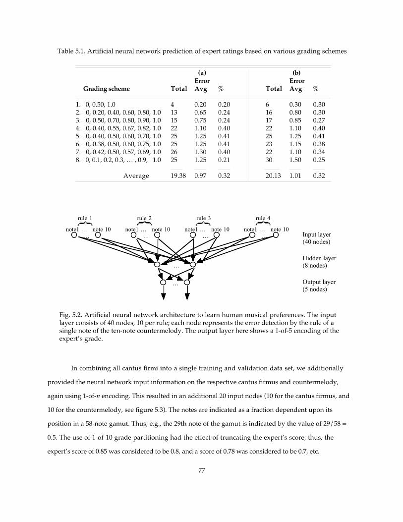
(a) (b) Error Error

Grading scheme Total Avg % Total Avg %

1. 0, 0.50, 1.0 4 0.20 0.20 6 0.30 0.302. 0, 0.20, 0.40, 0.60, 0.80, 1.0 13 0.65 0.24 16 0.80 0.303. 0, 0.50, 0.70, 0.80, 0.90, 1.0 15 0.75 0.24 17 0.85 0.274. 0, 0.40, 0.55, 0.67, 0.82, 1.0 22 1.10 0.40 22 1.10 0.405. 0, 0.40, 0.50, 0.60, 0.70, 1.0 25 1.25 0.41 25 1.25 0.416. 0, 0.38, 0.50, 0.60, 0.75, 1.0 25 1.25 0.41 23 1.15 0.387. 0, 0.42, 0.50, 0.57, 0.69, 1.0 26 1.30 0.40 22 1.10 0.348. 0, 0.1, 0.2, 0.3, … , 0.9, 1.0 25 1.25 0.21 30 1.50 0.25

Average 19.38 0.97 0.32 20.13 1.01 0.32

Table 5.1. Artificial neural network prediction of expert ratings based on various grading schemes

…note1 … note 10

… … …

…

…

Input layer(40 nodes)

Hidden layer(8 nodes)

Output layer(5 nodes)

rule 1 rule 2 rule 3 rule 4

note1 … note 10 note1 … note 10 note1 … note 10

Fig. 5.2. Artificial neural network architecture to learn human musical preferences. The input layer consists of 40 nodes, 10 per rule; each node represents the error detection by the rule of a single note of the ten-note countermelody. The output layer here shows a 1-of-5 encoding of the expert’s grade.

In combining all cantus firmi into a single training and validation data set, we additionally

provided the neural network input information on the respective cantus firmus and countermelody,

again using 1-of-n encoding. This resulted in an additional 20 input nodes (10 for the cantus firmus, and

10 for the countermelody, see figure 5.3). The notes are indicated as a fraction dependent upon its

position in a 58-note gamut. Thus, e.g., the 29th note of the gamut is indicated by the value of 29/58 =

0.5. The use of 1-of-10 grade partitioning had the effect of truncating the expert’s score; thus, the

expert’s score of 0.85 was considered to be 0.8, and a score of 0.78 was considered to be 0.7, etc.

77

…note1 … note 10

… … …

…

…

Input layer(60 nodes)

Hidden layer(15 nodes)Output layer(5 nodes)

counter-melody rule 1 rule 2 rule 3

note1 … note 10 note1 … note 10 note1 … note 10…

cantus firmus

note1 … note 10…

rule 4

note1 … note 10

Fig. 5.3. Artificial neural network with input information on cantus firmus and countermelody. The output layer here shows a 1-of-5 encoding of the expert’s grade.

Example 5.1. The following shows (a) a training exemplar represented as (b) a string of values in [0, 1] (here spaced across several lines for clarity) for neural net input and output nodes. In (b), the first row is the error detection by the Tonality, Final in Leaps of Fourths and Fifths, False Relations, and Note Variety rules, represented as 10-bit vectors; e.g., the first two rules detected no errors, but the False Relations rule detected an error in the sixth and eighth notes of the countermelody. The next two rows show the cantus firmus and the countermelody , and the final row shows the expert’s score in 1-of-10 representation.

(a) countermelody/cantus firmus expert’s scoreD E D E G F E F a G 0.65d c h c h a h a F# G

(b) 0 0 0 0 0 0 0 0 0 0 0 0 0 0 0 0 0 0 0 0 0 0 0 0 0 1 0 1 0 0 1 1 0 1 1 1 0 0 0 0 0.534483 0.482759 0.465517 0.482759 0.465517 0.413793 0.465517 0.413793 0.344828 0.362069 0.241379 0.293103 0.241379 0.293103 0.362069 0.310345 0.293103 0.310345 0.413793 0.362069 0 0 0 0 0 0 1 0 0 0 �

We have also trained the neural network using partially filled countermelodies (more on this

latter topic in section 5.2.1). See appendix C, section C.2 for the input data formatted using partially

filled countermelodies.

It should be noted that the function computed by the artificial neural network is implicit: there

is no way to derive the actual weights (i.e., wR in formula [2]), or even to determine the nature, linear

or otherwise, of the computation of the overall merit of a countermelody. It is also not possible to

analyze precisely the complexity of this method.

All told, training an artificial neural network is more an art than a science. We can suggest

several training variations: train the network on a more restricted rule set by asking the expert to

78

evaluate countermelodies based only on given criteria (note variety, smoothness of melody, etc.);

restrict training sets to one or two different cantus firmi only; train using non-experts whose

discriminatory powers may not be as acute as those of an expert’s but may show decided preferences

nevertheless. Regarding the latter, experiments on non-experts suggest, for example, that certain

individuals evaluate exemplars based solely on tessitura (average pitch of a melody): one subject

manifestly preferred low-lying melodies, while in contrast another individual preferred just the

opposite.

Despite their unique difficulties, artificial neural networks have a singular advantage in that

they are robust mechanisms in the face of noisy or contradictory data—quite appropriate for use in our

situation, as music experts are notoriously inconsistent. For example, music experts often rate two very

similar melodies very differently, and this poses a problem if the available rules are not able to

distinguish the two melodies; to differentiate exemplars as much as possible, we have suggested

inputting not only the rule evaluations, but also information on the cantus firmus and countermelody;

this results in a more comprehensive feature set.

5.2.1. Non-Increasing Scores of Partial Countermelodies

We intend to use the evaluations of a trained network in algorithms to produce countermelodies, using

the best-first and genetic algorithms (chapter 6). If using the neural network for countermelody

evaluations, both algorithms naturally expect the network to evaluate complete countermelodies; the

best-first algorithm, in addition, requires the network to evaluate partial countermelodies (see

algorithm 6.2). Since the original training data was based on the expert’s evaluations of complete

countermelodies, we need to extend the training data set to give the network the ability to evaluate

partial countermelodies as well.

Here is the method we used to prepare partial countermelodies and their appropriate scores:

for each exemplar, based on a single n-note cantus firmus, create n-1 exemplars comprising the same

expert rating together with the partial melodies consisting of the [nth], [(n-1)th, n th], [(n-2)th, (n-

1)th, and nth], … , [2nd, 3rd, … , and nth] notes of the original melody, respectively. We use this

enhanced training set to train the network to output the same grade for any partial countermelody as for

the complete countermelody. See appendix C, section C.2 for an example of a data set configured this

way (using only training and validation examples in the mixolydian mode).

79

Such a trained network can then be used in the best-first branch-and-bound algorithm without

contradiction of one of the algorithm’s requirements: that the predicted score should be non-increasing

as we descend a branch on the search tree. This is because partial countermelodies tend to have fewer

rule violations, and hence a higher score, than would a longer countermelody lower down in the same

branch of the search tree. As appendix E, section E.3 shows, a network trained with partial

countermelodies clearly produces more consistent evaluations with respect to partial countermelodies

than does one trained only on complete countermelodies.

5.3. Summary

In order to be convincingly human-like, music produced algorithmically must reflect human preferences.

We describe two methods to achieve this. Performing the Jeppesen Experiment, we weight a set of

selected fuzzy rules to reflect an expert’s value system; adopting a machine learning approach, we train

an artificial neural network by an expert’s grading of a set of countermelodies, using the diagnosis of

artistry rules. Certain aspects of the Jeppesen Experiment involves yet another set of intractable

problems, shown to be such by reduction from INTEGER PROGRAMMING and KNAPSACK.

In artificial neural network training, partitioning of the grades according to various grading

schemes affects prediction accuracy. Non-increasing grades of partial countermelodies, with respect to

the length of these countermelodies, is also a vital issue if the network’s output is to be used in the best-

first branch-and-bound algorithm, described in the next chapter.

80

CHAPTER 6. HEURISTIC ALGORITHMS BASED ON FUZZY RULE APPLICATION

When faced with difficult problems like those described in chapter 4, we have four options. The first

option is simply to avoid such problems entirely. The second is to solve easier versions of these

problems: this we have done by identifying those versions that are solvable efficiently by finite state

transducers (chapter 3). The third is to attempt only small instances of the intractable problem: solve

for short cantus firmi, for which even exhaustive search does not take intolerably long a time to

complete. The fourth is to find approximate algorithms and settle for near-optimal countermelodies.

We describe here two heuristic methods for the third and fourth options.

The first of our two heuristic methods applies a best-first search with branch-and-bound

pruning. It improves upon a straightforward “generate-and-test” exhaustive tree search with pruning,

which is the “brute-force” approach that serves as a benchmark for proposed improvements in all

search algorithms. The second method applies a genetic algorithm to obtain approximately optimal

results. This method adapts an algorithm based on biological evolutionary principles that has been

used successfully in many optimization problems. Although we originally designed our methods to solve

the optimization problem of composing counterpoint, they can easily be adapted to solve the other

three problems we have identified, viz., decision, enumeration, and number.

Both heuristic methods use fuzzy rule application (chapter 2, section 2.3). We can choose among

using either the weighted average of all fuzzy rules (applying formula[2.3], with all rules equally

weighted, with weights individually adjusted, or determined by means of the method described in the

Jeppesen Experiment), or the output of a trained artificial neural network. For the implementation of

these methods, see appendix D, sections D.2–3.

6.1. Best-First Search with Branch-and-Bound Pruning Algorithm

The best-first search with branch-and-bound pruning algorithm is an improvement over an exhaustive

search algorithm. Exhaustive algorithms are rarely practical for all but small instances. Yet, they

serve usefully as a benchmark against which other, possibly more efficient, algorithms can be

measured. We therefore first describe an exhaustive algorithm for the species counterpoint problem.

Our version of the exhaustive algorithm performs a tree search method with pruning (the

generate-and-test method) and incorporates the notion of crisp and fuzzy rule application. We apply

the set of crisp rules to every note that is considered in the construction of a countermelody. At any point

in the construction of this countermelody, as soon as a crisp rule is broken, we abandon that (partial)

81

countermelody, and backtrack to consider another countermelody. In this way, we avoid exploring many

futile branches. If, however, a fuzzy rule is broken, we keep a tally on the frequency of violation of that

rule. A countermelody that does not break any crisp rules emerges with a score depending on the degree

it satisfies all the fuzzy rules. We may thus rank all “correct” countermelodies. We can also express the

merit of a countermelody by an interval of values representing a “fuzzy” score; in this case we can adopt

the preference ranking method based on a fuzzy measure of “leftness” relations (Kundu 1997). For the

derivation of such values, and the application of preference ranking, see Gwee (1998).

Algorithm 6.1 shows a recursive implementation of the generate-and-test algorithm. See

appendix D, section D.2.1 for a more efficient iterative implementation of this algorithm.

Algorithm GenerateAndTest Input: finite set of notes S, cantus firmus CF. Output: list of melodies L.1. for each note n ∈ S 2. Extend m by adding n as a prefix3. if m does not satisfy all the rules

Remove n from m else

if m is a complete melody Add a copy of m to L Remove n from m

elseGenerateAndTest (S, CF).

Algorithm 6.1. Generate-and-test algorithm to produce valid countermelodies (L) to cantus firmus CF

Example 6.1. Figure 6.1 shows the search tree for the generation of countermelodies to cantus firmus <D, E, C#, D>. Numbers above each node indicate the depth-first order in which the node was created. The algorithm generates countermelodies in reverse and paths starting from leaves at the lowest level to the topmost level nodes represent “correct” countermelodies. In this example, the algorithm found five correct countermelodies: <D, C, E, D>, <a, E, E, D>, <a, G, E, D>, <D, E, e, d>, and <d, c, e, d>. Numbers in leaf nodes of correct countermelodies indicate the score of that countermelody. Thus, the optimal countermelodies are <D, C, E, D> and <d, c, e, d>, with a score of 0.97. �

Pruning in the manner illustrated in example 6.1 enables us to abandon fruitless searches on

extensions of any faulty substrings. Besides pruning, we have found other means of improving upon the

straightforward exhaustive search. We may order the rules to apply the more selective rules before

the less selective ones: since once any rule is broken in the construction of a countermelody, no further

application of other rules or further exploration of the countermelody is necessary. For example, it may

be expedient to allow such a (computationally) simple rule as the Dissonant Harmonic Intervals Rule to

82

evaluate a proposed countermelody before most other rules, owing to its high selectivity (see chapter 2,

section 2.1.1). Such ordering of the rules, while cutting down on extraneous rule application, will not

improve the efficiency of the search algorithm by any order of magnitude. For this to happen, we still

need to be able to prune the search tree more extensively and preferably at higher levels.

D a d

E

A C E G h e

D.97

d.97

a.94

D.94

a.91

e

E c e g hh

1

2

3 4

5

6

7

8

9

10

12 13

14

15

16

1711 18

19

20 21 22

h

Fig. 6.1. Search tree for the generation of countermelodies to the cantus firmus <D, E, C#, D>. Paths starting from leaves at the lowest level to the topmost level nodes represent “correct” countermelodies. There are five correct countermelodies, and two optimal countermelodies: <D, C, E, D> and <d, c, e, d>. The two optimal countermelodies have a score of 0.97. Nodes are labeled 1, 2 … 19 in the depth-first order.

We can facilitate such earlier pruning by constructing countermelodies in reverse: the cadence

rules (Final Cadence Rule and Approach to Cadence Rule) are among the most selective of the rules and

can eliminate many branches very early on; Lewin’s Rule (Lewin 1983), another relatively selective

rule, can be most effective if applied to a reversed countermelody (example 6.2).

Example 6.2. Consider the following (grammatically incorrect) melody:

a F G a b a G F D

The error lies in the last two notes of the melody: the cadence rules and Lewin’s Rule require that the penultimate note be a step away from the final note (here, only E or C# would be valid). If this melody were built in the normal order (i.e., successively a, F, G, etc.), very many alternatives will be considered correct, until the penultimate note is reached. In this case, all alternatives with F and D as the final pair of notes would ultimately be rejected. On the other hand, if this melody were built in reverse (i.e., successively D, F, etc.), no branch extending beyond the sequence D–F would be admitted. Here in fact only branches extending beyond D–E and D–C# would be considered. �

In sum, if a melody were built front to back (as illustrated in example 6.2), very many alternatives

present themselves at the beginning, many of which will ultimately be rejected; if the melody were

83

built back to front, very few alternatives are correct at the outset, and fewer fruitless branches will be

explored.

The difference in the number of nodes visited during the search between a forward and a reverse

scanning order is drastically shown in example 6.3, which illustrates the benefits in search efficiency of

early pruning of the search tree brought about by searching a reverse melody with application of rules

that are extremely selective on the ending portion of the melody.

(a )

Level Nodes searched:

1 56

2 562 = 3136

3 563 = 175616

4 56 * 175616 = 9834496

Total: 10013304

C# E

FF aaa…

FF aaa… FF aaa…

C# EC# E C# E

DD D D D D D D

(b)

… …

…………

D

C# E

FF

aaaaaa

aaa aaa aaa aaa

FF

FF FF FF

FF

Level Nodes searched:

1 56

2 56

3 56 * 2 = 112

4 56 * 112 = 6272

Total: 6496

Fig. 6.2. Comparison of the number of nodes visited during the search of a four-note countermelody with a gamut of 56 notes, given the application of only the cadence rules in (a) forward order; (b) reverse order

Example 6.3. Figure 6.2 illustrates the number of nodes searched in forward and reverse order, respectively. A forward order search examined 10013304 nodes, while a reverse order search examined only 6496. �

84

The best-first search algorithm improves upon the exhaustive search by selectively exploring

branches of the search tree (algorithm 6.2). Unlike the exhaustive search, which systematically, but

blindly, searches branches in a set order (e.g., leftmost- and depth-first), the best-first search tries its

best to avoid fruitless explorations by applying fuzzy rule heuristics. Use of these heuristics also

enables the user to abbreviate the search by specifying a threshold fuzzy rating, or to ask for only the m

best melodies.

Algorithm BestFirst Input: finite set of notes S , cantus firmus CF. Output: optimal_melody.1. for each note n ∈ S

Create partial melody m by making n its first noteif bound (m, CF) > 0 // bound computes the merit of m w.r.t. CF,

node := <m , bound (m, CF) > // and returns 0 if m is ungrammaticalEnqueue node into priority queue PQ // priority based on bound (m, CF ) and |m |

2. found := false3. optimal_melody := blank4. while not found and PQ is not empty

Dequeue node from PQ // priority queue ensures the best is chosen firstif |node .m | < |CF |

for each note n in SCreate partial melody m’ from node . m extended by addition of n if bound (m’, CF) > 0

node2 := < m’, bound (m’, CF) > Enqueue node2 into PQ

elseoptimal_melody := node .mfound := true.

Algorithm 6.2. Best-first algorithm to produce an optimal countermelody to cantus firmus CF

The algorithm performs a best-first search and places a bound on each node by calculating the

fuzzy score of the partial countermelody (see figure 6.3). The bounds computed are such that they are

non-increasing with the level of the nodes, and are therefore upper bounds. In case of a tie in the bounds

between nodes in the same level, the lexicographical ordering prevails, and between nodes at different

levels, the node at the lower level is chosen for expansion. The rationale for the latter criterion is that

melodies nearer completion stand a better chance of obtaining the best ultimate score.

Example 6.4. The pruned search tree produced for the cantus firmus <D, E, C#, D> is shown in figure 6.3 (compare the search tree traversed by the exhaustive algorithm for the same cantus firmus, figure 6.1). Stored in each node are the musical note and the bound, with only nodes of non-zero bounds shown; as with figure 6.1, the numbers above each node indicate the order in which the nodes are created. This algorithm in general explores fewer nodes than does the exhaustive algorithm: in this instance, nodes in lighter shade were not explored. The optimal countermelodies are: <D, C, E, D> and

85

<d, c, e, d>. For output of the best-first and genetic algorithms to the cantus firmus <D, F, E, D, G, F, a, G, F, E, D>, using rules weighted to favor Jeppesen’s preferences, see appendix B (output for num blanks = 11) and appendix E, section E.1. �

D1

a1

d1

E1

A.94

C.97

E.94

G.94

h.91

e.94

D.97

d.97

a.94

e1

E.94

h.91

c.97

e.97

g.94

hh.91

1 2 3

4

5 6 7 8 9 10 12 13 14 15 16 17

11

18 1920

Fig. 6.3. Pruned search tree produced by the branch-and-bound algorithm for cantus firmus <D, E, C#, D>. Paths starting from leaves at the lowest level to the topmost level nodes represent “correct” melodies. Optimal countermelodies here are <D, C, E, D> and <d, c, e, d>.

To evaluate complete countermelodies and to calculate the bounds of partial countermelodies,

we may use the output of an artificial neural network trained to reflect an expert’s preferences. As we

pointed out in chapter 5, section 5.2.1, if we do so, we need to preserve the integrity of the best-first

search algorithm: it is crucial that the artificial neural network produce non-increasing scores with

respect to any partial countermelody when descending a particular branch of the search tree. We have

attempted to train networks to produce consistent scores in this respect (see appendices C and E, sections

C.2 and E.3). Despite our best intentions in training the neural network with partial melodies, however,

it turned out that its evaluations were not always non-increasing. In our implementation of the best-

first algorithm, we had to allow for this, and so directed the algorithm to keep open the possibility

that a more recent complete melody may actually have a higher score than an earlier one; if

evaluation scores were absolutely non-increasing, the algorithm could assume that no more recently

completed melody could ever be better than previous ones. See appendix E, section E.3.1 for an instance

where a neural network not producing non-increasing output misleads the best-first algorithm into

outputting suboptimal countermelodies ahead of some optimal ones, subverting the mechanism behind

its main advantage over an exhaustive search. On the other hand, a neural network trained on data

86

prepared as described in chapter 5, section 5.2.1 (almost) succeeds in producing non-increasing output

with respect to the partial countermelodies; the best-first algorithm that uses such a neural network

runs (almost) as expected, with (most) optimal countermelodies output before suboptimal ones

(appendix E, section E.3.2).

Example 6.5. The best-first search algorithm produced the following optimal countermelodies to the cantus firmus <d, c, h, c, h, a, h, a, F#, G>. The evaluation function used a neural network trained on the same cantus firmus. The grading scale was based on the 0–0.2–0.4–0.6–0.8–1.0 partitioning, which gave about the best predictive ability (see chapter 5, section 5.2). The third countermelody (<D, E, G, F, G, F, E, F, a, G>) actually also belonged to the validation set used in the training of the network; using the current grading scale, the expert gave the same grade to this countermelody. The absence of an “A”-grade countermelody might be due to the fact that the highest grade obtained for all training data corresponding to this cantus firmus was only a “B”.

Countermelody Grade1. D E G E G F E F a G "B"2. D F G E G F E F a G "B"3. D E G F G F E F a G "B"4. D F G F G F E F a G "B"5. D E G E G F G F a G "B"6. G E G E G F G F a G "B"7. D F G E G F G F a G "B"8. d e g e g f g f aa g "B" �

6.2. Genetic Algorithm

Both the exhaustive and branch-and-bound algorithms conduct thorough and deterministic searches.

The common enemy of both these algorithms is the combinatorial explosion of the search space size;

their dedication to thoroughness condemns both algorithms to long and possibly fruitless searches.

Using a completely different search method, genetic algorithms model evolutionary processes to search

equally large spaces in less thorough but more expedient ways. In part randomized, these algorithms

use historical information to set up favorable conditions for promising solutions to manifest themselves.

In its most common implementation, a genetic algorithm maintains a set of strings each encoding

a candidate solution to the problem (in genetic algorithm terminology, a population of chromosomes).

Each candidate solution is assessed according to some fitness criterion. Through an iterative process,

solutions that are “more fit” stand a better chance of preservation than those that are “less fit”; fitter

solutions also stand a better chance of participating in the creation of new candidate solutions (in

biological systems, these correspond to survival and reproduction). It is hoped that in the course of

many iterations (epochs), a steadily improving set of solutions emerges, ultimately resulting in an

optimal or near-optimal solution.

87

We have developed a system using the genetic algorithm to produce approximately optimal

counterpoints to given cantus firmi. The chromosomes represent the candidate melodies and the genes

are the various notes themselves: thus, the four-gene chromosome “D C E D” represents the melody <D,

C, E, D>. In our implementation, we have used the technique of fitness scaling (Goldberg 1989, 76) to

avoid premature convergence (see appendix D, algorithm D.5).

The basic genetic algorithm randomly generates an initial population. If all possible encodings

are valid, then all chromosomes produced are also valid. In the case of species counterpoint, however,

valid chromosomes (corresponding to countermelodies) are not necessarily musically valid: in the

majority of cases, the countermelody would violate one or more crisp rules. By our system of melodic

evaluation, such randomly produced chromosomes would form initial populations with very low,

probably zero, average fitness. Subsequent epochs would result in no better than random string

generation. In order to give the algorithm a more promising start, we introduce domain specific

modifications not just to ensure valid strings, but also to create highly diversified initial populations

with relatively high average fitness (as far as reasonably possible). We do so by allowing several

initialization attempts for each chromosome, with the hope of producing at least some chromosomes

with non-zero fitness. With initial non-zero fitness populations, we then have the option of retaining

optimal melodies in future generations using the elitist model, or we may store such optimal melodies so

that, even if they do not survive, we ultimately will have all optimal melodies that have been

created during the execution of the algorithm. The sample outputs of the genetic algorithm in appendix

E, sections E.1–2 all show non-zero fitness initial populations.

As we had for the best-first algorithm we have here several options for evaluation functions.

Burton and Vladimirova (1999) classify music composition genetic algorithm systems by the evaluation

functions they use: deterministic mathematical functions (Horner and Goldberg 1991; Ralley 1995); user-

determined (Biles 1994; Horowitz 1994); formalistic, i.e., rule-based (McIntyre 1994; Horner and Ayers

1995; Thywissen 1996); and neural network-based (Gibson and Byrne 1991).

We have used evaluation functions characterizing the latter two classifications listed above,

and our functions are based on methods described in chapter 5. The rule-based evaluation functions use

fuzzy rules weighted to favor Jeppesen’s choice for the cantus firmus <D, F, E, D, G, F, a, G, F, E, D> (see

chapter 5, section 5.1). Two runs of the genetic algorithm succeeded in producing the optimal

88

countermelody: <a, aa, g, f, e, d, c, h, d, c#, d> (this was also Jeppesen’s choice). The first run took seven

iterations, while the second took only three (appendix E, section E.1).

Example 6.6. We illustrate below how crossover and selection operations produced the optimal countermelody <a, aa, g, f, e, d, c, h, d, c#, d> in the second run of the genetic algorithm to the cantus firmus <D, F, E, D, G, F, a, G, F, E, D> (only the ancestors to the optimal countermelody are shown here):

Generation Countermelody Fitness Operation AncestryInitial 0. a aa g f e f e h d c# d 0.87 INITIAL 4. aa d g f e f e h d c# d 0.84 INITIAL

11. d a e f e d c h d c# d 0.80 INITIAL14. d c e f e d c h d c# d 0.78 INITIAL18. a a h d e d c h d c# d 0.76 INITIAL19. d d c d e d c h d c# d 0.75 INITIAL

1. 0. a aa g f e f e h d c# d 0.87 CROSSOVER 0 4 2. aa d g f e f e h d c# d 0.84 SELECTION 4

11. d a e f e d c h d c# d 0.80 CROSSOVER 19 1114. d c e f e d c h d c# d 0.78 CROSSOVER 14 18

2. 1. a aa g f e f e h d c# d 0.87 CROSSOVER 2 017. d c e f e d c h d c# d 0.78 CROSSOVER 14 11

3. 0. a aa g f e d c h d c# d 0.89 CROSSOVER 17 1 �

We may also make arbitrary weight assignments. In this latter case, we could give equal

weights to all but perhaps one of the fuzzy rules to see if by giving emphasis to that one rule, whether

the set of optimal melodies could change. Not unexpectedly, this was found to be so (example 6.7).

Example 6.7. We compare the outputs of the best-first search and genetic algorithms to cantus firmus <D, F, E, D, G, F, a, G, F, E, D> (Jeppesen 1931, 112). The best-first algorithm produced the same optimal countermelodies to satisfy (a) rules equally weighted, and (b) rules weighted to give preference to the Stepwise Motion Rule, but a different optimal countermelody when (c) the Note Variety Rule was given preference. In comparison, the genetic algorithm quite quickly produced the same optimal countermelodies with equally weighted rules (further illustrated in figure 6.4). The grade for each countermelody is the weighted average of the individual rule scores.

Best-first algorithm

(a) Equally weighted fuzzy rulesCountermelody Grade

1. aa aa g f e d c e d c# d 0.8890912. a a G F E D C E D C# D 0.8890913. a a G F E D C B D C# D 0.8890914. aa aa g f e d c h d c# d 0.889091

89

(b) Preference for Stepwise Motion Rule1. aa aa g f e d c e d c# d 0.8931822. a a G F E D C E D C# D 0.8931823. a a G F E D C B D C# D 0.8931824. aa aa g f e d c h d c# d 0.893182

(c) Preference for Note Variety Rule1. a aa g f e d c h d c# d 0.861364

Genetic algorithm

crossover rate: 0.6mutation rate: 0.1max num initialization attempts: 20max num crossover attempts: 20max num mutation attempts: 20fitness multiple: 1.2population size: 100max num iterations: 50

Countermelody Grade Iteration 1. a a G F E D C E D C# D 0.89 Initial population2. a a G F E D C B D C# D 0.89 Initial population3. aa aa g f e d c h d c# d 0.89 24. aa aa g f e d c e d c# d 0.89 3 �

It is not surprising, however, that the genetic algorithm does not always produce optimal solutions to

instances of the species counterpoint problem, or all the possible optimal solutions. Perhaps more

typical are the results shown in example 6.8.

Example 6.8. The following is the output of the genetic algorithm to cantus firmus <D, F, E, D, G, F, a, G, F, E, D> (same cantus firmus as for example 6.7), evaluated by (a) equally weighted rules, rules weighted with preference for (b) Stepwise Motion, and for (c) Note Variety, respectively:

(a) Equally weighted fuzzy rules Countermelody Grade Iteration 1. a aa g f e d c h d c# d 0.89 19

(b) Preference for Stepwise Motion Rule 1. d d e f e d c h d c# d 0.87 26

(c) Preference for Note Variety Rule 1. aa aa g f e a c h d c# d 0.85 8 �

The other evaluation function we used is based on a trained neural network that reflects the

choice of one particular expert, and exploits the diagnostic feedback of fuzzy rules. In order to generate

good rhythms, Gibson and Byrne (1991) rely on the proximity of candidate rhythms to “good” ones to

guide their evaluations; but in order to generate good countermelodies, similarly relying on the

90

proximity of candidate countermelodies to “good” ones as an indication of fitness is extremely risky. See

example 2.7 for an illustration of the difference a single semitone can make to a countermelody.

0.9

0.8

0.7

0.6

0.5

0.4

0.3

0.2

0.1

Fitness

Iteration

0 1 2 3 4 5 6 7 8 9 1 0 1 1 1 2 1 3 1 4 1 5 1 6 1 7 1 8 1 9 2 0 2 1 2 2 2 3 2 4 2 5 2 6 2 7 2 8 2 9 3 0

Average population fitness

a a G F E D C E D C# Da a G F E D C B D C# D

aa aa g f e d c h d c# d

aa aa g f e d c e d c# d

Fig. 6.4. Generation of optimal countermelodies by the genetic algorithm to cantus firmus <D, F, E, D, G, F, a, G, F, E, D>

Example 6.9. The genetic algorithm produced the following optimal countermelodies to the cantus firmus <d, c, h, c, h, a, h, a, F#, G>, the same one for which the best-first algorithm produced the output shown in example 6.5. The evaluation function was carried out by the same trained neural network as for the best-first algorithm. For the initial population, each chromosome was allowed a maximum of 50 initialization attempts to produce a countermelody of non-zero fitness. With relatively short cantus firmi, this often results in several very fit chromosomes in the initial population: notice the presence of several optimal countermelodies in the initial population. Notice also the speed with which the set of eight optimal countermelodies was produced (fig. 6.5). This set is the same set as that produced by the best-first algorithm.

crossover rate: 0.6mutation rate: 0.1max num initialization attempts: 50max num crossover attempts: 20max num mutation attempts: 20fitness multiple: 1.2population size: 50

91

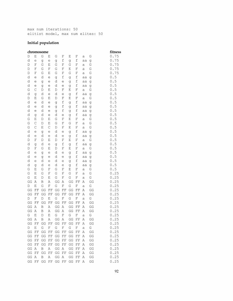
max num iterations: 50elitist model, max num elites: 50

Initial population

chromosome fitness D E G E G F E F a G 0.75 d e g e g f g f aa g 0.75 D F G E G F G F a G 0.75 D F G F G F E F a G 0.75 D F G E G F G F a G 0.75 d e d e g f g f aa g 0.5 d e g e d e g f aa g 0.5 d e g e d e g f aa g 0.5 G C D E D F E F a G 0.5 d g d e d e g f aa g 0.5 D E G E D F E F a G 0.5 d e d e g f g f aa g 0.5 d e d e g f g f aa g 0.5 d e d e g f g f aa g 0.5 d g d e d e g f aa g 0.5 G E D E G F E F a G 0.5 G C D E G F G F a G 0.5 G C E C D F E F a G 0.5 d e g e d e g f aa g 0.5 d e d e d e g f aa g 0.5 D F D E D F E F a G 0.5 d g d e g f g f aa g 0.5 D F G E D F E F a G 0.5 d e g e d e g f aa g 0.5 d e g e d e g f aa g 0.5 d e d e d e g f aa g 0.5 d g d e d e g f aa g 0.5 G E G F G F E F a G 0.5 G E G F G F G F a G 0.25 G E D E G F G F a G 0.25 GG A B A GG A GG FF A GG 0.25 D E G F G F G F a G 0.25 GG FF GG FF GG FF GG FF A GG 0.25 GG FF GG FF GG FF GG FF A GG 0.25 D F D E G F G F a G 0.25 GG FF GG FF GG FF GG FF A GG 0.25 GG A B A GG A GG FF A GG 0.25 GG A B A GG A GG FF A GG 0.25 G E D E G F G F a G 0.25 GG A B A GG A GG FF A GG 0.25 GG FF GG FF GG FF GG FF A GG 0.25 D E G F G F G F a G 0.25 GG FF GG FF GG FF GG FF A GG 0.25 GG FF GG FF GG FF GG FF A GG 0.25 GG FF GG FF GG FF GG FF A GG 0.25 GG FF GG FF GG FF GG FF A GG 0.25 GG A B A GG A GG FF A GG 0.25 GG FF GG FF GG FF GG FF A GG 0.25 GG A B A GG A GG FF A GG 0.25 GG FF GG FF GG FF GG FF A GG 0.25

92

Countermelody Grade Iteration 1. D E G E G F E F a G "B" Initial population2. d e g e g f g f aa g "B" Initial population 3. D F G E G F G F a G "B" Initial population 4. D F G F G F E F a G "B" Initial population 5. D E G F G F E F a G "B" 26. G E G E G F G F a G "B" 2 7. D F G E G F E F a G "B" 2 8. D E G E G F G F a G "B" 7 �

0.8

0.7

0.6

0.5

0.4

Fitness

Iteration

0 1 2 3 4 5 6 7 8 9 1 0 1 1 1 2 1 3 1 4 1 5 1 6 1 7 1 8 1 9 2 0 2 1 2 2 2 3 2 4 2 5 2 6 2 7 2 8 2 9 3 0

Average population fitness

D E G E G F E F a Gd e g e g f g f aa g D F G E G F G F a G D F G F G F E F a G

D E G F G F E F a GG E G E G F G F a GD F G E G F E F a G

D E G E G F G F a G

Fig. 6.5. Generation of optimal countermelodies by the genetic algorithm to cantus firmus <d, c, h, c, h, a, h, a, F#, G>. The average fitness of the population was derived by the same process of “grade-point averages” used in schools and colleges to convert letter grades to numerical scores.

In using a trained neural network as the fitness evaluator, we are limited to chromosomes of

length equal to the length of the cantus firmi used in the training of the network, since the architecture

of the network was initially determined by this length. Furthermore, for the best predictive ability,

we need to use cantus firmi that are not too different from the ones used in the training of the network.

Further experiments with more cantus firmi can extend the utility of this evaluation method.

93

We compared the performance of the genetic algorithm with a quasi-random algorithm that at

each iteration randomly generated a new population. While this random algorithm succeeded in

producing some reasonably good countermelodies, it took a long time to do so, since for each randomly

produced population a considerable number of attempts were necessary to ensure that the constituent

chromosomes represented valid countermelodies. The genetic algorithm, on the other hand, (quasi-)

randomly generated a population only at the beginning; for the rest of the time, its evolutionary

processes took over and in a relatively short time produced a variety of good countermelodies. Also, the

genetic algorithm always produced populations with higher average fitness than did the randomized

algorithm.

Example 6.10. The following is output of the random algorithm for the same cantus firmus as for example 6.7 (<D, F, E, D, G, F, a, G, F, E, D>). The random algorithm ran for 200 iterations, generating one countermelody per iteration, and was allowed 20 attempts per countermelody. Weighted rules gave preference for stepwise motion. Shown are the progressively better countermelodies generated in the course of the algorithm: only one optimal countermelody was found (iteration 124).

Countermelody Grade Iteration 1. aa d g f g d f e d c# d 0.74 22. aa f g f e a c h d c# d 0.75 83. d d c f g d f e d c# d 0.78 134. a a G F C D F E D C# D 0.85 645. aa aa g f e d c e d c# d 0.89 124 �

In the above outputs of the genetic algorithm, it will be observed that we began with the

benefit of reasonably fit initial populations, thanks to the multiple initialization attempts at creating

valid chromosomes. Even so, there is no guarantee that all initial populations have a reasonable level

of fitness. Unless we spend an inordinate amount of time in generating an initial population by

increasing the number of initialization attempts, it may still be possible that initial populations have

very low fitness. This is especially true of more complex species (like second species), or of species with

more than one added part, where for each cantus firmus, they are very more possible countermelodies

compared to our simple first species with one added part.

Example 6.11. We performed two runs of the genetic algorithm to cantus firmus <D, a, G, F, E, D, F, E, D> (Jeppesen 1931, 117) to produce counterpoint in second species with one added part, and in first species with two added parts. The initial populations for both runs had very low fitness, and in both cases contained only a single chromosome that actually had a non-zero fitness. Yet, with the elitist model, the valid initial chromosomes survived and thus seized the opportunity to foster more and more valid and fit offspring.

In the run to produce second species with one added part, despite an initial population of low average fitness (for more details see appendix E, section E.2.1), the genetic algorithm succeeded in finding several near-optimal countermelodies. Several rules had to be fuzzified in order to render

94

Jeppesen’s solution valid (Lewin’s, Recovery, Outline Tritone in Four, Harmonic Range, Unisons, and Simultaneous Leaps Rules); these rules returned an aggregate score of 0.99 for Jeppesen’s solution. The following shows the final population, and Jeppesen’s solution. Figure 6.6 illustrates the generation of the optimal countermelodies.

Countermelody Grade Iteration 1. a f c d e E a b c G F a D F E C# D 0.99 162. d f c d e E a b c G F a D F E C# D 0.99 223. a f c d e h a b c G F a D F E C# D 0.99 224. a f c d e E a h c G F a D F E C# D 0.99 265. a f c d e d a b c G F a D F E C# D 0.99 276. d f c d e h a b c G F a D F E C# D 0.99 297. a d c d e E a b c G F a D F E C# D 0.99 308. a f c d e h a h c G F a D F E C# D 0.99 329. a b c f e E a b c G F a D F E C# D 0.99 3410. d f c d e E a h c G F a D F E C# D 0.99 4011. a d c d e h a h c G F a D F E C# D 0.99 4112. d f c d e d a b c G F a D F E C# D 0.99 4113. d f c d e h a h c G F a D F E C# D 0.99 4414. a f c d e h a d c G F a D F E C# D 0.99 4615. d b c f e E a b c G F a D F E C# D 0.99 4616. d f c d e d a h c G F a D F E C# D 0.99 4617. a h c d e E a b c G F a D F E C# D 0.99 4818. a b c f e E a h c G F a D F E C# D 0.99 4919. a b c d e E a b c G F a D F E C# D 0.99 4920. a d c d e h a b c G F a D F E C# D 0.99 50

Jeppesen’s solution

a h c d e d f F G a b F a h c# - d 0.99

In the run to produce counterpoint in first species with two added parts, the genetic algorithm again produced several near-optimal countermelodies, despite a poor start (for more details see appendix E, section E.2.2). Here also, several rules had to be fuzzified in order to render Jeppesen’s solution valid (Lewin’s, Stepwise Motion, Recovery, Unisons, and Simultaneous Leaps Rules); these rules returned an aggregate score of 0.91 for Jeppesen’s solution. Figure 6.7 illustrates the generation of the optimal countermelodies.

Countermelody pair Grade Iteration

1. D D G a G F D C# D d d e f c d aa a d 0.92 18

2. D D G a G F D C# D d d e d c d aa a d 0.92 34

Jeppesen’s solution

d c e f g aa d c# d D F E D E F a A D 0.91 �

95

1

0.9

0.8

0.7

0.6

0.5

0.4

0.3

0.2

0.1

0

Fitness

Iteration

0 1 2 3 4 5 6 7 8 9 1 01 11 21 31 41 51 61 71 81 92 02 12 22 32 42 52 62 72 82 93 03 13 23 33 43 53 63 73 83 94 04 14 24 34 44 54 64 74 84 95 0

Average population fitness

a f c d e E a b c G F a D F E C# D

d f c d e E a b c G F a D F E C# D a f c d e h a b c G F a D F E C# D

a f c d e E a h c G F a D F E C# D

a f c d e d a b c G F a D F E C# D

d f c d e h a b c G F a D F E C# D

a d c d e E a b c G F a D F E C# D

a f c d e h a h c G F a D F E C# D

a b c f e E a b c G F a D F E C# D

d f c d e E a h c G F a D F E C# D

a d c d e h a h c G F a D F E C# D d f c d e d a b c G F a D F E C# D

d f c d e h a h c G F a D F E C# D

a f c d e h a d c G F a D F E C# D d b c f e E a b c G F a D F E C# D d f c d e d a h c G F a D F E C# D

a h c d e E a b c G F a D F E C# D

a b c f e E a h c G F a D F E C# D a b c d e E a b c G F a D F E C# D

a d c d e h a b c G F a D F E C# D

Fig. 6.6. Generation of optimal countermelodies by the genetic algorithm to cantus firmus <D, a, G, F, E, D, F, E, D> (second species, two parts)

96

0.9

0.8

0.7

0.6

0.5

0.4

0.3

0.2

0.1

0

Fitness

Iteration0 1 2 3 4 5 6 7 8 9 1 01 11 21 31 41 51 61 71 81 92 02 12 22 32 42 52 62 72 82 93 03 13 23 33 43 53 63 73 83 94 04 14 24 34 44 54 64 74 84 95 0

Average population fitness

D D G a G F D C# D d d e f c d aa a d

D D G a G F D C# D d d e d c d aa a d

Fig. 6.7. Generation of near-optimal countermelodies by the genetic algorithm to cantus firmus <D, a, G, F, E, D, F, E, D> (first species, three parts)

6.2.1. Musical Gestures and Schemata

Applying the genetic algorithm to music composition requires justification. We have tried to provide

some by comparing its performance with a random generation of countermelodies (example 6.10). In this

section, we consider how the Schema Theorem (Holland 1975) might provide a mathematical

characterization of the process of countermelody generation by, and hence another justification for, the

genetic algorithm.

Consider again the countermelodies generated in example 6.6 (cantus firmus <D, F, E, D, G, F, a,

G, F, E, D>, with rules weighted to favor Jeppesen’s preferences). Examining the various substrings that

constitute the optimal countermelody found in the third generation (<a, aa, g, f, e, d, c, h, d, c#, d>), we

observe that the following substrings figure prominently in previous generations: “a aa …”, “… g f e

…”, and “… h d c# d”. They are present, not only in the above ancestral strings, but also in other highly

fit strings, as can be verified from appendix E, listing E.2.

These observations are quite consistent with the Schema Theorem, in which context the three

substrings can be characterized respectively as schemata (similarity templates) (a) “a aa * * * * * * *

97

* *”, (b) “* * g f e * * * * * *”, and (c) “* * * * * * * h d c# d”, where the symbol ‘*’ indicates “don’t

care.” These schemata represent well-known musical gestures (short, easily recognizable phrases):

schema (a) is the opening octave leap; schema (b) is simply the descending scale pattern outlining a

third; and schema (c) is a common cadential pattern in the dorian mode. These three schemata qualify

as building blocks (fit schemata [based on the average fitness of all its representative strings] with

short defining lengths [distance between the first and last specific string position]). Of these, schema

(a) is among the fittest and shortest of the schemata throughout the first three generations; its length

is in fact the shortest for schemata that represent meaningful musical gestures. The fittest schema with

the longest defining length and highest order (number of fixed positions) present in these generations is

“a aa g f e * * h d c# d”. This schema can be described musically as a pattern beginning with an

opening octave leap followed by stepwise motion in the opposite direction (as per the “strict” form of

the Recovery Rule), and closing with a well-known dorian mode cadential pattern: most musicians will

agree that this makes for a very satisfying melody.

The Schema Theorem estimates, for a particular schema, a lower bound on the number of

chromosomes representing this schema at a particular generation. This estimate is based on several

factors: crossover and mutation rates, and, in the previous generation, the number of chromosomes

representing this schema, average fitness of all chromosomes representing this schema, and average

fitness of all chromosomes. Thus:

Estlower [m (s, t)] ≥ (fs (t - 1)/fpop (t - 1) ) m (s, t - 1) [1 - pc (defLen (s)/(len - 1) )] (1 - pm)order (s) (6.1)

whereEstlower [m (s, t)] is the lower-bound estimate of the number of chromosomes representing schema s at generation t, fs (t - 1) is the average fitness of all chromosomes representing schema s at generation t - 1, fpop (t - 1) is the average fitness of all chromosomes in the population at generation t - 1, m (s, t - 1) is the number of chromosomes representing schema s at generation t - 1, pc is the crossover rate (0 ≤ pc ≤ 1), defLen (s) is the defining length of schema s, len is the length of the chromosome, pm is the mutation rate (0 ≤ pm ≤ 1), order (s) is the order of schema s.

The Schema Theorem estimates only the lower bound because it considers only the destructive aspects of

the crossover and mutation operations. By considering otherwise, we can estimate the upper bound as

follows:

98

Estupper [m (s, t)] = (a) estimate of the number of chromosomes representing s selected into generation t + (b) estimate of the number of chromosomes resulting from the crossover operation

involving chromosomes representing s + (c) estimate of the number of chromosomes resulting from the crossover operation

involving chromosomes not representing s + (d) estimate of the number of chromosomes resulting from the mutation operation

involving chromosomes not representing s

In (b), we assume that the crossover operation does not destroy any representative of schema s. We also

assume that the mutation operation does not destroy any representative of s surviving into the current

generation. On the other hand, we shall ignore the relatively low probability that the crossover and

mutation operations will produce a chromosome representing schema s ([c] and [d]). Then,

(a) = (fs (t - 1)/fpop (t - 1) ) m (s, t - 1) (1 - pc)(b) = (fs (t - 1)/fpop (t - 1) ) m (s, t - 1) (pc)

Thus, we arrive at an estimate of the upper bound:

Estupper [m (s, t)] ≤ (fs (t - 1)/fpop (t - 1) ) m (s, t - 1) (6.2)whereEstupper [m (s, t)] is the upper-bound estimate of the number of chromosomes representing schema s at generation t, fs (t - 1) is the average fitness of all chromosomes representing schema s at generation t - 1, fpop (t - 1) is the average fitness of all chromosomes in the population at generation t - 1, m (s, t - 1) is the number of chromosomes representing schema s at generation t - 1.

Example 6.12. Figures 6.8–10 compare lower- and upper-bound estimates of the number of occurrences of schema (a) “a aa * * * * * * * * *”, (b) “* * g f e * * * * * *”, and (c) “* * * * * * * h d c# d”, during the first 20 iterations of a genetic algorithm run to the cantus firmus <D, F, E, D, G, F, a, G, F, E, D> (example 6.6). For each of the schemata, the actual number of representatives compares quite closely to the lower- and upper-bound estimates.

Figure 6.11 compares average fitnesses of the population, and the three schemata. The increase of average fitness of representatives of the schemata corresponds to the increase of the average population fitness. Notice that in this instance, the schema with the shortest defining length and order (“a aa * * * * * * * * *”) also tends to have the highest average fitness.

An unfortunate mutation occurring in the ninth generation produced a zero-fitness chromosome (“a aa g f e d c e d c# d”). The mutation operation apparently altered the fourth gene from the end (from “h” to “e”), which resulted in a chromosome that represented the first two schemata but excluded the third. This explains the dip in the average fitnesses of the first two schemata in the ninth generation, from which recovery was immediate (fig. 6.11). Compare also the effect on the upper- and lower-bound estimates for these schemata (figs. 6.8–10).

See appendix E, table E.1 for the schemata fitnesses, population fitness, and schemata occurrences used to derive the bounds estimates (equations 6.1–2). �

99

2 0

1 0

0

quantity

generation

1 2 3 4 5 6 7 8 9 10 11 12 13 14 15 16 17 18 19 20

schema "a aa * * * * * * * * *"

lower bound

upper bound

actual m (s, t)

Fig. 6.8. Lower- and upper-bound estimates of the number of occurrences of schema “a aa * * * * * * * * *” during the first 20 iterations of a genetic algorithm run to the cantus firmus <D, F, E, D, G, F, a, G, F, E, D>

2 0

1 0

0

quantity

generation

1 2 3 4 5 6 7 8 9 10 11 12 13 14 15 16 17 18 19 20

schema "* * g f e * * * * * *"

lower bound

upper bound

actual m (s, t)

Fig. 6.9. Lower- and upper-bound estimates of the number of occurrences of schema “* * g f e * * * * * *” during the first 20 iterations of a genetic algorithm run to the cantus firmus <D, F, E, D, G, F, a, G, F, E, D>

100

2 0

1 0

0

quantity

generation

1 2 3 4 5 6 7 8 9 10 11 12 13 14 15 16 17 18 19 20

schema "* * * * * * * h d c# d"

lower bound

upper bound

actual m (s, t)

Fig. 6.10. Lower- and upper-bound estimates of the number of occurrences of schema “* * * * * * * h d c# d” during the first 20 iterations of a genetic algorithm run to the cantus firmus <D, F, E, D, G, F, a, G, F, E, D>

0.890.880.870.860.850.840.830.820.81

0.80.790.780.770.760.750.740.730.72

Average fitness

Generation

0 1 2 3 4 5 6 7 8 9 1 01 11 21 31 41 51 61 71 81 92 0

Fitness comparison

population

"a aa *********"

"**g f e******"

"*******h d c# d"

Fig. 6.11. Comparison of the average fitnesses of the population and of schema (a) “a aa * * * * * * * * *”, (b) “* * g f e * * * * * *”, and (c) “* * * * * * * h d c# d” during the first 20 iterations of a genetic algorithm run to the cantus firmus <D, F, E, D, G, F, a, G, F, E, D>

101

The Schema Theorem was one of the first attempts to justify mathematically the efficacy of

genetic algorithms. Here, we have observed how it may characterize the creation of countermelodies.

We believe that these albeit brief observations warrant further research on the relationship between

musical gestures and schemata.

6.3. Exhaustive and Heuristic Algorithms Compared

The exhaustive generate-and-test method suffers from two drawbacks: it is impractical for long cantus

firmi, and even for short ones, one has to wait for the algorithm to produce the entire set of correct

countermelodies before being able to evaluate their relative merit. The best-first search with branch-

and-bound pruning algorithm addresses both drawbacks by its selective exploration of the search tree.

This algorithm, in conjunction with fuzzy rule application, produces countermelodies in order of merit

(based on preference criteria of a particular listener), and avoids wasting time searching for inferior

countermelodies. At the worst, however, this algorithm degenerates to an exhaustive search: it may

turn out that the heuristics are not effective to begin with, or else a particular cantus firmus may defeat

all attempts at smart searching. Also, we have seen that its selective search ability is seriously

undermined if its evaluation function (such as a trained neural network) fails to produce non-increasing

scores along any path down the search tree.

Both the exhaustive search and the best-first algorithms guarantee optimal solutions, but the

latter still takes a very long time to process cantus firmi of any significant length. The exhaustive

search technique quickly yields a considerable number of solutions, but since it does not produce them in

order of merit, one must still wait for the entire set of countermelodies before sorting them. The genetic

algorithm often appears the best compromise, producing near-optimal solutions in a relatively short

time. On the other hand, some runs may not produce even a single successful counterpoint. See appendix

E for sample outputs of the best-first and genetic algorithms, using various evaluation methods (trained

neural network, and explicitly weighted rules).

Implementations of these methods will not only be useful in helping the musician by producing

high quality countermelodies that can be subsequently assessed or verified according to criteria of

interest to the expert, but can also be used to solve other complexity-related problems. For example, the

rules and gamut can easily be modified to solve, among other problems, the Three-Dimensional

Matching problem. We do so along the lines of the transformation we described (chapter 4, section 4.1.2)

in the NP-completeness proof: we write a system to create first species with two added parts, with an

102

appropriate gamut, and create rules that ensure all notes are distinct. We can even have an

optimization version of the matching problem, where various matchings can have different

“happiness” ratings, and the goal is to find the happiest matching.

6.4. Summary

Exhaustive searches for valid countermelodies are practical only for short cantus firmi, owing to the

intractability of the problem. Two heuristic algorithms to solve the species counterpoint optimization

problem are the best-first branch-and-bound, and genetic algorithms. In these algorithms, fuzzy rule

application provides the basis for heuristic searches.

Experiments with various rule weightings, including that produced by a simplified application

of the Jeppesen Experiment, produced promising results. So also with the output of a trained neural

network. If its output is to be used in the best-first algorithm, however, the issue of non-increasing scores

of partial countermelodies in the network output needs to be observed.

103

CHAPTER 7. CONCLUSION

In this dissertation, we investigated machine intelligence applied to music. Using species counterpoint

as our musical model, we examined both theoretical and practical aspects of algorithmic music

composition. We related general music problems to a vast realm of difficult problems by deriving their

complexity classes. We formalized various species counterpoint problems as decision, enumeration,

number, and optimization problems. We then proved NP-completeness, #P-completeness, “strong sense”

NP-completeness, and NP-equivalence of these formalized problems, inferring that efficient solutions

of these music problems give us efficient solutions of many other problems, including NP and NP-

complete problems. On the other hand, the addition of these music problems to the growing lists of NP-

complete and related problems lends further weight to the strong belief among researchers that P ≠ NP.

We showed how restricted versions of the decision problem can be solved efficiently by using

the finite state machine model. Straightforward extensions to the basic finite state model enabled us to

solve enumeration, number, and even optimization versions of the decision problem, and also to output

desired countermelodies. We then investigated what specific aspects render these problems unsolvable

not only by finite state machines, but also insolvable efficiently by any computational model at all.

Producing even one correct countermelody for a cantus firmus is thus a non-trivial problem. But

even more interesting is the challenge of producing human-like music. To meet this challenge, we

formulated new rules for species counterpoint, called “artistry” rules, and proposed fuzzy rule

application to represent more accurately the intent and nature of these and other rules. We argued that

this extension to crisp rule application enabled us to approximate human musical preferences, and we

supported our claim by performing experiments to tune the weights of fuzzy rules directly by means of

the “Jeppesen Experiment” and indirectly by backpropagation neural network learning. We thereby

obtained heuristic measures, which can then be used in solving more general and intractable problems.

To solve the intractable music optimization problem, we developed programs using two

algorithms: a branch-and-bound optimizing algorithm, and an adaptation of genetic algorithms as an

approximating alternative to the branch-and-bound algorithm. In these algorithms, the tuned fuzzy

rules guide the search process.

We now summarize the key ideas expressed, and contributions made, in this dissertation:

a) Fuzzy application of existing rules as a basis of artistic machine composition of music. Such

application of certain rules is truer to their spirit than their traditional crisp treatment.

104

b) New “artistry rules” to reflect modern tastes in music. These rules are especially suitable for fuzzy

application and for use in machine learning of human musical tastes.

c) Efficient solution of restricted decision, enumeration, number, and optimization problems using the

finite state machine model. We showed how to construct finite state machines to implement certain

types of rules that are amenable to efficient solutions.

d) Intractability of the general compositional problem and related problem classes. We distinguished

which kinds of problems are intractable, and which are not. For those that are intractable, we proved

their intractability, thus showing their close connection with interesting non-musical problems.

e) Intractability of the generalized rule redundancy and rule indispensability problem. Simple but

suboptimal rule elimination is tractable, but the general optimization problem is not.

f) Methods to reflect human musical preferences. We outlined a procedure to capture the rule

preferences of an expert by an iterative process of rule weight tuning. The general problem of weight

tuning is non-trivial, and in some formulations, even intractable. On the other hand, artificial neural

network training offers a more efficient but suboptimal solution. We outlined a procedure to train a

backpropagation neural network to reflect an expert’s preferences through fuzzy rule input.

g) Heuristic algorithms to produce human-like musical compositions, using possibly the above methods

of reflecting human musical preferences. We explored the use of genetic algorithms and found that its

performance compared favorably with exhaustive and best-first search algorithms.

7.1. Future Work

Results from the application of our artistry rules suggest that several more need to be identified. This

would enable a more accurate description of human musical preferences, and promote more

comprehensive feature input for neural network training. In addition to rules whose weightings can be

adjusted to reflect human preferences, we could also devise methods to tune these and other rules to

reflect the element of surprise or thwarted expectation that characterize great musical works;

apparently the desire to be surprised is deeply rooted in nature (Werner and Todd 1997).

From a music theoretic standpoint, we might consider whether any of the numerous rules are

redundant, or what would be a sufficient subset of the rules. As we have indicated, this problem in

general is intractable. As shown for the intractable compositional problems, we could perhaps be less

ambitious here, too. In chapter 2, we showed a way to measure the selectivity of rules, and we could use

this data to optimize the order of rule application to reduce somewhat the computational demands in

105

evaluating candidate countermelodies. What would be desirable are more correctness rules that

eliminate shorter partial candidate countermelodies that would in any case be eliminated further

down in the search tree.

Our theoretical discussions have largely centered around time-complexity issues. There

remains, however, a vast amount of space-complexity issues still waiting to be explored with respect to

the music compositional, and perhaps the rule redundancy, problems. Specifically, the issues involve

log space and P-space completeness. This is quite significant because P-space completeness is an even

stronger measure of intractability than is NP-completeness. Also interesting is the question whether

the transformations we used in the NP-completeness and related proofs are also log space

transformations. Jones (1973) and Stockmeyer and Meyer (1973) have observed that the polynomial

transformations used in most NP-completeness proofs are also log-space transformations.

We have presently developed application programs for a subset of the instructional corpus of

species counterpoint, namely, first and second species: two and three parts, fourth species: two parts.

Although they illustrate satisfactorily the hypotheses we made, it would be interesting to see how

these algorithms scale up to the more complex species, especially fifth species with more than two

parts.

Species counterpoint is a pedagogical basis for more concrete musical styles. We would like to

see how our analysis applies to these other styles, in particular, four-part common-practice harmony,

and two- and three-part counterpoint in the style of J. S. Bach. The exponential difficulty should be

even more apparent in these more complicated styles. The overriding factor remains human artistry.

106

REFERENCES

Ames, Charles. 1982. Protocol: Motivation, design, and production of a composition for solo piano. Interface 11(4):213–238.

____. 1983. Stylistic automata in Gradient. Computer Music Journal 7(4):45–56.

Bezdek, J. C. 1981. Pattern recognition with fuzzy objective function algorithms. New York: Plenum Press.

Biles, John A. 1994. GenJam: A genetic algorithm for generating jazz solos. Proceedings of the 1994 International Computer Music Conference. 131–137. San Francisco, CA: International Computer Music Association.

Borosh, I., and L. B. Treybig. 1976. Bounds on positive integral solutions of linear Diophantine equations. Proceedings of the American Mathematical Society, vol. 55 no. 2, 299–304.

Burton, Anthony R., and Tanya Vladimirova. 1999. Generation of musical sequences with genetic techniques. Computer Music Journal 23(4):59–73.

Camurri, Antonio, Giovanni De Poli, and Davide Rocchesso. 1995. A taxonomy for sound and music computing. Computer Music Journal 19(2):4–5.

Cook, Stephen A. 1971. The complexity of theorem-proving procedures. Proceedings of the Third Annual ACM Symposium on Theory of Computing. 151–158. New York: Association for Computing Machinery.

Dantzig, G. B. 1963. Linear programming and extensions. Princeton, N. J.: Princeton University Press.

Dobkin, D., R. Lipton, and S. Reiss. 1976. Linear programming is P-complete. Excursions into geometry, same authors, Report No. 71, Department of Computer Science, Yale University. New Haven, CT.

Ebcioglu, Kemal. 1988. An expert system for harmonizing four-part chorales. Computer Music Journal 12(3):43–51.

Floyd, Robert W. 1962. Algorithm 97: Shortest path. Communications of the ACM 5 (6):345.

Fux, Johann Joseph. 1725. Gradus ad parnassum. Translated by Alfred Mann. Steps to Parnassus: The Study of Counterpoint. Revised edition, 1965. London: Dent.

Garey, Michael R., and David S. Johnson. 1978. Strong NP-completeness results: Motivation, examples, and implications. Journal of the ACM 25:499–508.

____. 1979. Computers and intractability: A guide to the theory of NP-completeness. 20th printing, 1999. New York: Freeman.

Gibson, P. M., and J. A. Byrne. 1991. Neurogen, Musical composition using genetic algorithms and co-operating neural networks. Proceedings of the Second International Conference on Artificial Neural Networks. 309–313. Stevenege, England: Institute of Electrical Engineers.

107

Goldberg, David E. 1989. Genetic algorithms in search, optimization, and machine learning. Reading, MA: Addison-Wesley.

Gross, Dorothy. 1984. Computer applications to music theory: A retrospective. Computer Music Journal 8(4):35–42.

Guido of Arezzo. [1025–26 or 1028–32] 1955. Micrologus (Little discourse). Edited by Joseph Smits van Waesberghe. Corpus scriptorum de musica 4. Rome: American Institute of Musicology.

Gwee, Nigel. 1998. Fuzzy techniques in rule-based composition of species counterpoint. Master’s thesis, Louisiana State University, Baton Rouge.

____. 2001. An NP-complete music problem. Proceedings of the 39th annual ACM-SE Conference. 184–190. Athens, GA.

____. 2002a. Capturing human musical preferences with fuzzy application of rules. Proceedings of the 40th annual ACM-SE Conference. 139–146. Raleigh, NC.

____. 2002b. Effective heuristics for algorithmic music composition. Proceedings of the International Conference on Artificial Intelligence. Vol. III. 1027–1033. Las Vegas, NV.

Hiller, Lejaren A., Jr., and Leonard M. Isaacson. 1959. Experimental music: Composition with an electronic computer. New York: McGraw-Hill.

Holland, John H. 1975. Adaptation in natural and artificial systems. Ann Arbor, MI: University of Michigan Press. Reprinted Cambridge, MA: MIT Press (1992).

Hörnel, Dominik. 1998. A multi-scale neural-network model for learning and reproducing chorale variations. Melodic similarity: Concepts, procedures, and applications. Computing in musicology 11. Edited by Walter B. Hewlett and Eleanor Selfridge-Field. Cambridge, MA: MIT Press. 141–157.

Horner, Andrew, and Lydia Ayers. 1995. Harmonization of musical progressions with genetic algorithms. Proceedings of the 1995 International Computer Music Conference. 483–484. San Francisco, CA: International Computer Music Association.

Horner, Andrew, and David E. Goldberg. 1991. Genetic algorithms and computer-assisted music composition. Proceedings of the 1991 International Computer Music Conference. 479–482. San Francisco, CA: International Computer Music Association.

Horowitz, Damon. 1994. Generating rhythms with genetic algorithms. Proceedings of the 1994 International Computer Music Conference. 142–143. San Francisco, CA: International Computer Music Association.

Jeppesen, Knud. 1931. Kontrapunkt (vokalpolyfoni). Copenhagen: Wilhelm Hansen. Translated by Glen Haydon, with a new introduction by Alfred Mann, as Counterpoint: The polyphonic vocal style of the sixteenth century. New York: Prentice-Hall (1939). Republished New York: Dover (1992).

Jones, N. D. 1973. Reducibility among combinatorial problems in log n space. Proceedings of the 7th Annual Princeton Conference on Information Sciences and Systems. 547–551.

108

Kannan, R., and C. L. Monma. 1978. On the computational complexity of integer programming problems. Lecture notes in economics and mathematical systems, 161–172. New York: Springer-Verlag.

Karmarkar, N. 1984. A new polynomial-time algorithm for linear programming. Combinatorica 4: 373–395.

Karp, Richard M. 1972. Reducibility among combinatorial problems. Complexity of Computer Computations. Edited by R. E. Miller and J. W. Thatcher. New York: Plenum Press. 85–104.

Khachiyan, L. G. 1979. A polynomial algorithm for linear programming. Doklady Akademii Nauk SSSR 244, 1093–1096. Translated in Soviet Math. Doklad 20, 191–194 (1979).

Kohonen, Teuvo. 1982. Self-organized formation of topologically correct feature maps. Biological Cybernetics 66:59–69.

____. 1984. Self-organization and associative memory. London: Springer-Verlag.

Kozen, D. 1977. Lower bounds for natural proof systems. Proceedings of the 18th Annual Symposium on Foundations of Computer Science, 254–266.

Kundu, Sukhamay. 1997. Min-transitivity of fuzzy leftness relationship and its application to decision making. Fuzzy Sets and Systems 86:357–367.

Lewin, David. 1983. An interesting global rule for species counterpoint. In Theory Only 6(8):19–44.

Lewis, Harry R., and Christos H. Papadimitriou. 1998. Elements of the theory of computation. Upper Saddle River, NJ: Prentice-Hall.

Mathews, Max V. 1965. Pitch quantizing for computer music. Journal of the Acoustical Society of America 38.

McIntyre, Ryan A. 1994. Bach in a box: The evolution of four-part baroque harmony using the genetic algorithm. Proceedings of the IEEE Conference on Evolutionary Computation. 852–857. Washington, DC: IEEE.

Mealy, G. H. 1955. A method for synthesizing sequential circuits. Bell System Technical Journal 34(5):1045–1079.

Moore, E. F. 1956. Gedanken experiments on sequential machines. Automata Studies. Princeton, NJ: Princeton University Press. 129–153.

Moret, Bernard M. 1997. The theory of computation. Reading, MA: Addison-Wesley.

Papadimitriou, Christos H. 1981. On the complexity of integer programming. Journal of the ACM 28(4):765–768.

____. 1995. Computational complexity. Reprint. Reading, MA: Addison-Wesley.

Ralley, David. 1995. Genetic algorithms as a tool for melodic development. Proceedings of the 1995 International Computer Music Conference. 501–502. San Francisco, CA: International Computer Music Association.

109

Roads, Curtis. 1980. Artificial intelligence and music. Computer Music Journal 4(2);13–25.

Sahni, Sartaj. 1974. Computationally related problems. SIAM Journal on Computing 3(4):262–279.

Schottstaedt, William. 1989. Automatic counterpoint. Current directions in computer music research, ed. Max V. Mathews and John R. Pierce, 199–214. Cambridge, MA: MIT Press.

Simon, Janos. 1975. On some central problems in computational complexity. PhD Thesis, Department of Computer Science, Cornell University, Ithaca, New York.

Stockmeyer, L. J., and A. R. Meyer. 1973. Word problems requiring exponential time. Proceedings of the 5th Annual ACM Symposium on Theory of Computing. 1–9.

Temperley, David, and Daniel Sleator. 1999. Modeling meter and harmony: A preference-rule approach. Computer Music Journal 23(1):10–27.

Thywissen, Kurt. 1996. GeNotator: An environment for investigating the application of genetic algorithms in computer-assisted composition. Proceedings of the 1996 International Computer Music Conference. 274–277. San Francisco, CA: International Computer Music Association.

Valiant, Leslie G. 1979. The complexity of computing the permanent. Theoretical Computer Science 8:189–201.

____. 1979b.The complexity of enumeration and reliability problems. SIAM Journal on Computing 8(3):410–421.

Werner, Gregory M., and Peter M. Todd. 1997. Too many love songs: Sexual selection and the evolution of communication. Proceedings of the Fourth European Conference on Artificial Life. 434–443. Cambridge, MA: MIT Press.

110

APPENDIX A. RULES OF SPECIES COUNTERPOINT

In section A.1 we describe the rules commonly used in first species counterpoint with one added part. In

section A.2 we show the output of the algorithm designed to discover indispensable rules, with respect

to specific cantus firmi.

A.1. Rules of First Species Counterpoint in Two Parts

We categorize these rules as “melody,” “harmony,” and “counterpoint.” We also list here under the

heading “Artistry Rules” four additional rules that we have proposed. The rules are described both

informally, and using if-then syntax.

A.1.1. Melody Rules

These rules govern the countermelody only: the cantus firmus is not affected by these rules. Some of the

rules prescribe what notes are allowed at certain positions in the countermelody, others describe the

relationship between adjacent notes, yet others affect notes with respect to the entire span of the

countermelody.

Table A.1. Melody rules of first species counterpoint in two parts

Rule Description

1. Rests Disallow rests.If note of the countermelody is pThen p is not rest.

2. Final Note The last note of a melody must be at the interval of either an octave,perfect fifth, or unison with the last note of the cantus firmus.If note of the cantus firmus is p and note' of the countermelody is q

and last (p) is true and last (q) is trueThen interval (p, q) is perfect octave

or interval (p, q) is perfect fifthor interval (p, q) is perfect unison.

3. Allow CertainFicta Notes

Allow C#, c#, cc#, Eb, eb, eeb, FF#, F#, f#, ff#, Bb.If note of the countermelody is p Then vera (p) is true

or p is C# or p is c# or p is cc# or p is Eb or p is eb or p is eebor p is FF# or p is F# or p is f# or p is ff# or p is Bb.

111

(table A.1 continued)

4. Ficta Notes In the dorian mode, the notes FF#, F#, f#, ff# are allowed if they lead bydownward step to the penultimate note of the melody. If the mode of the cantus firmus is dorian and antepenultimate(countermelody) is FF#|F#|f#|ff#Then penultimate (countermelody) is EE|E|e|ee.

5. B flats Allow Bb, b, and bb only in the dorian mode.If note of the countermelody is p and the mode of the cantus firmus is notdorianThen p is not Bb and p is not b and p is not bb.

6. Lewin’s For every non-final note p of a melody, there should exist a note q between p and the final note r of the melody such that the musicalinterval p–q is a descending step if p is higher than r, and an ascendingstep if p is lower than r. If noten of the countermelody is p

and final (countermelody) is rand higher than (p, r) is true

Then exists (q = noten+i of the countermelody) and lower than (q, p) and interval size (p, q) is second.

If noten of the countermelody is p and final (countermelody) is rand lower than (p, r) is true

Then exists (q = noten+i of the countermelody) and higher than (q, p) and interval size (p, q) is second.

7. Melodic Range Disallow a melodic range exceeding a 13th.If the lowest note of the countermelody is p and the highest note of thecountermelody is qThen greater than ( interval size (p, q), thirteenth) is false.

8. DissonantMelodicIntervals

Disallow augmented or diminished intervals.If noten of the countermelody is p and noten+1 of the countermelody is q Then the interval type (p, q) is major or the interval type (p, q) is minor.

9. OtherInadmissibleIntervals

Disallow compound intervals, 7ths, or ascending leaps of a major 6th. If noten of the countermelody is p and noten+1 of the countermelody is q Then less than (interval size (p, q), ninth)

and not interval size (p, q) is seventh and not (interval (p, q) is major sixth

and ascending (p, q) ).

112

(table A.1 continued)

10. Repeated NotesOnce Only

Allow repeated notes only once in the course of a melody. If noten of the countermelody is p and noten+1 of the countermelody is q

and notem of the countermelody is r and notem+1 of thecountermelody is s and p = q and r = s

Then n = m.

11. Repeated Notes Stronger version of Rule 9: disallow all repeated notes. If noten of the countermelody is p and noten+1 of the countermelody is q Then p ≠ q.

12. Successive MinorSeconds

Disallow successive minor 2nds.If noten of the countermelody is p and noten+1 of the countermelody is q

and noten+2 of the countermelody is r and interval (p, q) is minor second

Then interval (q, r) is not minor second.

13. Stepwise Motion Stepwise motion should predominate. (see also Note Variety rule)If number of steps (countermelody) is steps and number of leaps(countermelody) is leaps Then steps >> leaps.

14. Recovery A leap in one direction should be followed by motion in the oppositedirection. If noten of the countermelody is p

and noten+1 of the countermelody is q and noten+2 of the countermelody is r

Then if ascending (p, q) is true then descending (q, r) is true

and if descending (p, q) is true then ascending (q, r) is true.

15. More Than TwoLeaps inSuccession

Disallow more than two ascending/descending leaps in succession. If noten of the countermelody is p

and noten+1 of the countermelody is q and noten+2 of the countermelody is r and noten+3 of the countermelody is s and ( ( ascending (p, q) and ascending (q, r) and ascending (r, s) ) or (descending (p, q) and descending (q, r) and descending (r, s) )and greater than (interval size (p, q), second)and greater than (interval size (q, r), second)

Then greater than (interval size (r, s), second) is false.

113

(table A.1 continued)

16. Two Leaps inSuccession

Disallow two ascending/descending leaps in succession, in which thesecond is larger than the first. If noten of the countermelody is p

and noten+1 of the countermelody is q and noten+2 of the countermelody is r and ( ( ascending (p, q) and ascending (q, r) )

or (descending (p, q) and descending (q, r) ) )and greater than (interval size (p, q), second)and greater than (interval size (q, r), second)

Then greater than (interval size (q, r), interval size (p, q) ) is false.

17. Outline Tritonein Three

Disallow successions of three notes that outline the tritone. If noten of the countermelody is p

and noten+2 of the countermelody is q Then interval (p, q) is not augmented fourth.

18. Outline Tritonein Four

Disallow successions of four notes that outline the tritone. If noten of the countermelody is p

and noten+3 of the countermelody is q Then interval (p, q) is not augmented fourth.

19. Two Fourths orFifths

Disallow successions of fourths or fifths.If noten of the countermelody is p

and noten+1 of the countermelody is q and noten+2 of the countermelody is r

Then not (interval size (p, q) is fourth and interval size (q, r) is fourth )and not (interval size (p, q) is fifth and interval size (q, r) isf i f th )

20. Approach toCadence

Governs the correct approach to cadences in the respective modes. If antepenultimate (countermelody) is p and penultimate (countermelody)is q and final (countermelody) is r

and interval (q, r) is minor secondThen interval size (p, q) is second or (interval size (p, q) is third anddescending (p, q) is true and ascending (q, r) is true) or (interval size (p, q)is third and ascending (p, q) is true and descending (q, r) is true).

21. Climax Disallow more than one occurrence of the highest note of the melody. If noten of the countermelody is p

and notem of the countermelody is q and highest (p) is true and highest (q) is true

Then n = m.

114

(table A.1 continued)

22. ChromaticResolution

Chromatic notes must resolve. If noten of the countermelody is p

and noten+1 of the countermelody is q Then if sharped (p)

then ascending (p, q) is true and interval (p, q) is minor second

and if flatted (p)then descending (p, q) is true

and interval (p, q) is minor second.

23. DiatonicResolution

Sharped notes must resolve by ascending step. If noten of the countermelody is p

and noten+1 of the countermelody is q Then if sharped (p)

then ascending (p, q) is true and interval (p, q) is minor second.

24. Symmetric Leaps A leap from a note in one direction should not be followed by leap in theopposite direction to that same note. If noten of the countermelody is p and noten+1 of the countermelody is qand noten+2 of the countermelody is r and greater than ( interval size (p,q), second) is true Then p ≠ r.

A.1.2. Harmony Rules

Harmony rules govern the relationships between notes of the cantus firmus and the countermelody. Only

notes of both parts that sound simultaneously are affected.

Table A.2. Harmony rules of first species counterpoint in two parts

Rule Description

1. HarmonicRange

Disallow more than one occurrence of the harmonic interval of thetwelfth. If noten of the cantus firmus is p

and noten of the countermelody is q and notem of the cantus firmus is r and notem of the countermelody is s and n ≠ m

Then not (interval size (p, q) is twelfth and interval size (r, s) istwelfth).

115

(table A.2 continued)

2. DissonantHarmonicIntervals

Disallow augmented and diminished harmonic intervals, and intervalsof the 2nd, 4th, 7th, 9th, and 11th.If noten of the cantus firmus is p and noten of the countermelody is q

and interval type (p, q) is pq and interval size (p, q) is pq_size Then pq is not augmented and pq is not diminished

and pq_size is not second and pq_size is not fourth and pq_size is not seventh and pq_size is not ninth and pq_size is not eleventh.

3. Unisons Disallow harmonic intervals of the unison except at the beginning or end. If noten of the cantus firmus is p and noten of the countermelody is q andinterval (p, q) is perfect unison Then n = 1 or n = length (cantus firmus).

4. PreservePentachord

The first harmonic interval should be either a unison, perfect fifth, oroctave.If note1 of the cantus firmus is p and note'1 of the countermelody is q

and interval (p, q) is pq Then pq is perfect unison of pq is perfect fifth or pq is perfect octave.

A.1.3. Counterpoint Rules

Counterpoint rules govern both the horizontal movement and vertical relationships of the

countermelody and the cantus firmus. These rules are local in nature, in that they govern a finite number

of notes at a time.

Table A.3. Counterpoint rules of first species counterpoint in two parts

Rule Description

1. ParallelFifths andOctaves

Disallow parallel perfect fifths and octaves.If noten of the cantus firmus is p and noten of the countermelody is q

and noten+1 of the cantus firmus is r and noten+1 of thecountermelody is s and the interval (p, q) is perfect fifth

Then the interval (r, s) is not perfect fifth. If noten of the cantus firmus is p and noten of the countermelody is q

and noten+1 of the cantus firmus is r and noten+1 of thecountermelody is s and the interval (p, q) is perfect octave

Then the interval (r, s) is not perfect octave.

116

(table A.3 continued)

2. ExposedFifths andOctaves

Disallow exposed fifths and octaves.If noten of the cantus firmus is p and noten of the countermelody is q

and interval size (p, q) is fifth or interval size (p, q) is octave Then exposed (p, q) is false.

3. ParallelThirds andSixths

Disallow more than five parallel thirds and sixths. If noten+i of the cantus firmus is pi+1 and noten+i of the countermelody isqi+1,

0 ≤ i ≤ 5and interval size (pi, qi) is third, 1 ≤ j ≤ 5

Then not (interval size (p6, q6) is third). If noten+i of the cantus firmus is pi+1 and noten+i of the countermelody isqi+1,

0 ≤ i ≤ 5and interval size (pi, qi) is sixth, 1 ≤ j ≤ 5

Then not (interval size (p6, q6) is sixth).

4. Simulta-neous Leaps

Disallow simultaneous leaps in the same direction in both the cantusfirmus and the added melody. If noten of the cantus firmus is p and noten of the cantus firmus is q

and noten+1 of the countermelody is r and noten+1 of thecountermelody is s and greater than (interval size (p, q), second) is true and greater than (interval size (r, s), second) is true

Then not (ascending (p, q) is true and ascending (r, s) is true) and not (descending (p, q) is true and descending (r, s) is true).

5. Simulta-neousFourths

Disallow simultaneous leaps of the fourth in both the cantus firmus andthe added melody.If noten of the countermelody is p and noten+1 of the countermelody is qand noten of the cantus firmus is r and noten+1 of the cantus firmus is s Then not (interval size (p, q) is fourth and interval size (r, s) is fourth).

117

(table A.3 continued)

6. FinalCadence

Enforces the cadential formulae for the various modes.If interval (penultimate (countermelody), penultimate (cantus firmus) ) ismajor sixth Then interval (final (countermelody), final (cantus firmus) ) is perfectoctave. If interval (penultimate (countermelody), penultimate (cantus firmus) ) isminor third Then interval (final (countermelody), final (cantus firmus) ) is perfectunison. If interval (penultimate (countermelody), penultimate (cantus firmus) ) isminor tenth Then interval (final (countermelody), final (cantus firmus) ) is perfectoctave. If interval (penultimate (countermelody), penultimate (cantus firmus) ) ismajor third Then interval (final (countermelody), final (cantus firmus) ) is perfectf i f th .

A.1.4. Artistry Rules

We present here four rules we have formulated to reflect preferences of an expert who contributed to

experiments we carried out to reflect human musical preferences (appendices B, C). These rules hold no

claim to historical accuracy, therefore.

Table A.4. Artistry rules of first species counterpoint in two parts

Rule Description

1. Tonality Melodies in the dorian and lydian modes should prefer b and bb over hand hh.If the mode of the cantus firmus is dorian or the mode is lydian Then any note of the countermelody is not h and is not hh.

2. Final inLeaps ofFourths andFifths

Leaps of fourths and fifths should preferably involve the final or itsoctave equivalent.If noten of the countermelody is p and noten+1 of the countermelody is q

and interval size (p, q) is fourth or interval size (p, q) is fifth Then p is final (cantus firmus) or q is final (cantus firmus)

or (interval (p, final (cantus firmus) ) is perfect octave) or (interval (q, final (cantus firmus) ) is perfect octave).

118

(table A.4 continued)

3. FalseRelations

In the dorian mode, notes C and c are best avoided if they occur close tothe cadence.In the mixolydian mode, notes F and f are best avoided if they occur closeto the cadence.If the mode of the cantus firmus is dorian and note of the countermelody isn and close to cadence (n) is true Then n is not C and n is not c. If the mode of the cantus firmus is mixolydian and note of thecountermelody is n and close to cadence (n) is true Then n is not F and n is not f.

4. NoteVariety

The same note should not be heard too many times in a melody.If for any note n of countermelody m, degree of repetition (n) is lowThen merit µnote variety of m is good. If for any note n of countermelody m, degree of repetition (n) is averageThen merit µnote variety of m is average. If for any note n of countermelody m, degree of repetition (n) is highThen merit µnote variety of m is poor.

A.2. Indispensable Rules with respect to Cantus Firmi <D, E, C#, D>, <a, D, F, E, D, C#, D>, and <D, F,E, D, G, F, a, G, F, E, D>

Using the algorithm described in chapter 2, section 2.1, we discovered the indispensable rules with

respect to the following three cantus firmi: <D, E, C#, D>, <a, D, F, E, D, C#, D>, and <D, F, E, D, G, F,

a, G, F, E, D>. The indispensable rules are those that, without which, at least one more countermelody

would have been admitted. Listings A.1–3 show the output of algorithm 2.1 applied on the three cantus

firmi.

Listing A.1. Output of algorithm 2.1 for cantus firmus <D, E, C#, D>

Cantus firmus: <D, E, C#, D>Gamut: {R, FF, GG, A, Bb, B, C, C#, D, E, F, G, a, b, h, c, c#, d, e, f, f#, g, aa}Alpha cut: 0

Rule ρ wTonality 1.0 1.0Final in Leaps of 4ths and 5ths 1.0 1.0False Relations 1.0 1.0 Note Variety 1.0 1.0

With all rules applied, No. countermelodies accepted: 2No. countermelodies analyzed: 184

countermelodiesRule disabled analyzed accepted uniquely rejected

1. Rests 184 2 02. Final Note 391 2 0

119

(listing A.1 continued)

3. Allow Certain Ficta Notes 184 2 04. Ficta Notes 230 4 25. B flats 184 2 06. Lewin’s 322 7 57. Melodic Range 184 2 08. Dissonant Melodic Intervals 184 2 09. Other Inadmissible Intervals 184 2 010. Repeated Notes Once Only 184 2 011. Repeated Notes 207 2 012. Successive Minor Seconds 184 2 013. Stepwise Motion 184 2 014. Recovery 184 2 015. More Than Two Leaps in Succession 184 2 016. Two Leaps in Succession 184 2 017. Outline Tritone in Three 184 2 018. Outline Tritone in Four 184 2 019. Two Fourths or Fifths 184 2 020. Approach to Cadence 184 2 021. Climax 184 2 022. Chromatic Resolution 184 2 023. Diatonic Resolution 184 2 024. Symmetric Leaps 184 2 025. Harmonic Range 184 2 026. Dissonant Harmonic Intervals 276 4 227. Unisons 184 2 028. Preserve Pentachord 184 6 429. Parallel Fifths and Octaves 184 2 030. Exposed Fifths and Octaves 184 2 031. Parallel Thirds and Sixths 184 2 032. Simultaneous Leaps 184 2 033. Simultaneous Fourths 184 2 034. Final Cadence 253 2 0

Indispensable rules for cantus firmus <D, E, C#, D>: 4. Ficta Notes6. Lewin’s26. Dissonant Harmonic Intervals28. Preserve Pentachord

Listing A.2. Output of algorithm 2.1 for cantus firmus <a, D, F, E, D, C#, D>

Cantus firmus: <a, D, F, E, D, C#, D>Gamut: {R, FF, GG, A, Bb, B, C, C#, D, E, F, G, a, b, h, c, c#, d, e, f, f#, g, aa}Alpha cut: 0

Rule ρ wTonality 1.0 1.0Final in Leaps of 4ths and 5ths 1.0 1.0False Relations 1.0 1.0 Note Variety 1.0 1.0

120

(listing A.2 continued)

With all rules applied, No. countermelodies accepted: 12No. countermelodies analyzed: 1012

countermelodiesRule disabled analyzed accepted uniquely rejected

1. Rests 1012 12 02. Final Note 1219 12 03 Allow Certain Ficta Notes 1012 12 04. CheckForFictaNotes 1679 25 135. B flats 1012 12 06. Lewin’s 5060 160 1487. Melodic Range 1012 12 08. Dissonant Melodic Intervals 1012 12 09. Other Inadmissible Intervals 1035 14 210. Repeated Notes Once Only 1012 12 011. Repeated Notes 1380 23 1112. Successive Minor Seconds 1012 12 013. Stepwise Motion 1012 12 014. Recovery 1012 12 015. More Than Two Leaps in Succession 1012 12 016. Two Leaps in Succession 1012 12 017. Outline Tritone in Three 1012 12 018. Outline Tritone in Four 1012 12 019. Two Fourths or Fifths 1012 12 020. Approach to Cadence 1012 12 021. Climax 1012 18 622. Chromatic Resolution 1104 14 223. Diatonic Resolution 1012 12 024. Symmetric Leaps 1035 14 225. Harmonic Range 1012 12 026. Dissonant Harmonic Intervals 4738 97 8527. Unisons 1357 13 128. Preserve Pentachord 1012 25 1329. Parallel Fifths and Octaves 1219 14 230. Exposed Fifths and Octaves 1012 12 031. Parallel Thirds and Sixths 1012 12 032. Simultaneous Leaps 1127 16 433. Simultaneous Fourths 1012 12 034. Final Cadence 1702 23 11

Indispensable rules for cantus firmus <a, D, F, E, D, C#, D>: 4. Ficta Notes6. Lewin’s9. Other Inadmissible Intervals11. Repeated Notes21. Climax22. Chromatic Resolution24. Symmetric Leaps26. Dissonant Harmonic Intervals

121

(listing A.2 continued)

27. Unisons28. Preserve Pentachord29. Parallel Fifths and Octaves32. Simultaneous Leaps34. Final Cadence

Listing A.3. Output of algorithm 2.1 for cantus firmus <D, F, E, D, G, F, a, G, F, E, D>

Cantus firmus: <D, F, E, D, G, F, a, G, F, E, D>Gamut: {R, FF, GG, A, Bb, B, C, C#, D, E, F, G, a, b, h, c, c#, d, e, f, f#, g, aa} Alpha cut: 0

Rule ρ wTonality 1.0 1.0Final in Leaps of 4ths and 5ths 1.0 1.0False Relations 1.0 1.0 Note Variety 1.0 1.0

With all rules applied, No. countermelodies accepted: 76No. countermelodies analyzed: 4853

countermelodiesRule disabled analyzed accepted uniquely rejected

1. Rests 4853 76 02. Final Note 5060 76 03. Allow Certain Ficta Notes 4853 76 04. CheckForFictaNotes 9499 206 1305. B flats 4853 76 06. Lewin’s 50324 1828 17527. Melodic Range 4853 76 08. Dissonant Melodic Intervals 6808 129 539. Other Inadmissible Intervals 5152 103 2710. Repeated Notes Once Only 4853 76 011. Repeated Notes 11730 129 5312. Successive Minor Seconds 4853 76 013. Stepwise Motion 4853 76 014. Recovery 4853 76 015. More Than Two Leaps in Succession 4853 76 016. Two Leaps in Succession 4853 76 017. Outline Tritone in Three 4853 76 018. Outline Tritone in Four 4853 76 019. Two Fourths or Fifths 4853 76 020. Approach to Cadence 4853 76 021. Climax 4853 117 4122. Chromatic Resolution 5842 107 3123. Diatonic Resolution 4899 76 024. Symmetric Leaps 6693 93 1725. Harmonic Range 4853 76 026. Dissonant Harmonic Intervals 1260032 31103 3102727. Unisons 12420 169 9328. Preserve Pentachord 4853 135 59

122

(listing A.3 continued)

29. Parallel Fifths and Octaves 7015 118 4230. Exposed Fifths and Octaves 6647 90 1431. Parallel Thirds and Sixths 4853 76 032. Simultaneous Leaps 9177 153 7733. Simultaneous Fourths 4853 76 034. Final Cadence 13041 248 172

Indispensable rules for cantus firmus <D, F, E, D, G, F, a, G, F, E, D>: 4. Ficta Notes6. Lewin’s8. Dissonant Melodic Intervals9. Other Inadmissible Intervals11. Repeated Notes21. Climax22. Chromatic Resolution24. Symmetric Leaps26. Dissonant Harmonic Intervals27. Unisons28. Preserve Pentachord29. Parallel Fifths and Octaves30. Exposed Fifths and Octaves32. Simultaneous Leaps34. Final Cadence

123

APPENDIX B. COUNTERPOINTS IN THE JEPPESEN EXPERIMENT

To the cantus firmus <D, F, E, D, G, F, a, G, F, E, D> one of Jeppesen’s solutions was <a, aa, g, f, e, d, c, h,

d, c#, d>, which we used to generate alternative countermelodies (see chapter 5, section 5.1). We

applied the rule weight vector <w1, w2, w3, w4> to the four artistry rules: <Tonality, Final in Leaps of

Fourths and Fifths, False Relations, Note Variety>. Shown below are the outputs for data sets

comprising partially filled countermelodies starting with one blank at each note position, followed

successively by partially filled countermelodies with two blanks, and so on. For each countermelody

generated, the output also shows the respective rule scores (1. Tonality; 2. Final in Leaps of Fourths and

Fifths; 3. False Relations; 4. Note Variety), followed by the aggregate scores. In all instances,

Jeppesen’s solution appears, and in most cases, as first in a list of alternatives, where more than one

alternative exists for the blank/s.

Listing B.1. Jeppesen’s countermelody and alternatives

Jeppesen’s Countermelody: <a, aa, g, f, e, d, c, h, d, c#, d>Cantus firmus: <D, F, E, D, G, F, a, G, F, E, D>

Output for data set with num blanks = 1, weight vector = <1, 1, 1, 1>:

Countermelody: Rule scores: 1. 2. 3. 4. Aggregate score

* aa g f e d c h d c# d1. a aa g f e d c h d c# d 0.91 1.00 0.91 0.82 0.912. aa - g f e d c h d c# d 0.91 1.00 0.91 0.73 0.89Number of solutions: 2. a * g f e d c h d c# d1. a aa g f e d c h d c# d 0.91 1.00 0.91 0.82 0.91Number of solutions: 1.

a aa * f e d c h d c# d1. a aa g f e d c h d c# d 0.91 1.00 0.91 0.82 0.91Number of solutions: 1.

a aa g * e d c h d c# d1. a aa g f e d c h d c# d 0.91 1.00 0.91 0.82 0.91Number of solutions: 1.

a aa g f * d c h d c# d1. a aa g f e d c h d c# d 0.91 1.00 0.91 0.82 0.91Number of solutions: 1.

a aa g f e * c h d c# d1. a aa g f e d c h d c# d 0.91 1.00 0.91 0.82 0.91Number of solutions: 1.

124

(listing B.1 continued)

a aa g f e d * h d c# d1. a aa g f e d e h d c# d 0.91 1.00 1.00 0.73 0.912. a aa g f e d c h d c# d 0.91 1.00 0.91 0.82 0.91Number of solutions: 2.

a aa g f e d c * d c# d1. a aa g f e d c h d c# d 0.91 1.00 0.91 0.82 0.91Number of solutions: 1.

a aa g f e d c h * c# d1. a aa g f e d c h d c# d 0.91 1.00 0.91 0.82 0.91Number of solutions: 1.

a aa g f e d c h d * d1. a aa g f e d c h d c# d 0.91 1.00 0.91 0.82 0.91Number of solutions: 1.

a aa g f e d c h d c# *1. a aa g f e d c h d c# d 0.91 1.00 0.91 0.82 0.91Number of solutions: 1.

Output for data set with num blanks = 1, weight vector = <1, 1, 1, 2>:

Countermelody: Rule scores: 1. 2. 3. 4. Aggregate score

* aa g f e d c h d c# d1. a aa g f e d c h d c# d 0.91 1.00 0.91 0.82 0.892. aa - g f e d c h d c# d 0.91 1.00 0.91 0.73 0.85Number of solutions: 2.

a * g f e d c h d c# d1. a aa g f e d c h d c# d 0.91 1.00 0.91 0.82 0.89Number of solutions: 1.

a aa * f e d c h d c# d1. a aa g f e d c h d c# d 0.91 1.00 0.91 0.82 0.89Number of solutions: 1.

a aa g * e d c h d c# d1. a aa g f e d c h d c# d 0.91 1.00 0.91 0.82 0.89Number of solutions: 1.

a aa g f * d c h d c# d1. a aa g f e d c h d c# d 0.91 1.00 0.91 0.82 0.89Number of solutions: 1.

a aa g f e * c h d c# d1. a aa g f e d c h d c# d 0.91 1.00 0.91 0.82 0.89Number of solutions: 1.

a aa g f e d * h d c# d1. a aa g f e d c h d c# d 0.91 1.00 0.91 0.82 0.892. a aa g f e d e h d c# d 0.91 1.00 1.00 0.73 0.87Number of solutions: 2.

a aa g f e d c * d c# d1. a aa g f e d c h d c# d 0.91 1.00 0.91 0.82 0.89Number of solutions: 1.

125

(listing B.1 continued)

a aa g f e d c h * c# d1. a aa g f e d c h d c# d 0.91 1.00 0.91 0.82 0.89Number of solutions: 1.

a aa g f e d c h d * d1. a aa g f e d c h d c# d 0.91 1.00 0.91 0.82 0.89Number of solutions: 1.

a aa g f e d c h d c# *1. a aa g f e d c h d c# d 0.91 1.00 0.91 0.82 0.89Number of solutions: 1.

Output for data set with num blanks = 2, weight vector = <1, 1, 1, 2>:

Countermelody: Rule scores: 1. 2. 3. 4. Aggregate score

* * g f e d c h d c# d1. a aa g f e d c h d c# d 0.91 1.00 0.91 0.82 0.892. aa - g f e d c h d c# d 0.91 1.00 0.91 0.73 0.853. aa d g f e d c h d c# d 0.91 1.00 0.91 0.73 0.854. aa f g f e d c h d c# d 0.91 1.00 0.91 0.73 0.855. d - g f e d c h d c# d 0.91 1.00 0.91 0.64 0.826. d c g f e d c h d c# d 0.91 0.91 0.91 0.64 0.80Number of solutions: 6.

a * * f e d c h d c# d1. a aa g f e d c h d c# d 0.91 1.00 0.91 0.82 0.892. a - e f e d c h d c# d 0.91 0.91 0.91 0.64 0.80Number of solutions: 2.

a aa * * e d c h d c# d1. a aa g f e d c h d c# d 0.91 1.00 0.91 0.82 0.89Number of solutions: 1.

a aa g * * d c h d c# d1. a aa g f e d c h d c# d 0.91 1.00 0.91 0.82 0.89Number of solutions: 1.

a aa g f * * c h d c# d1. a aa g f e d c h d c# d 0.91 1.00 0.91 0.82 0.89Number of solutions: 1.

a aa g f e * * h d c# d1. a aa g f e d c h d c# d 0.91 1.00 0.91 0.82 0.892. a aa g f e f e h d c# d 0.91 1.00 1.00 0.73 0.873. a aa g f e d e h d c# d 0.91 1.00 1.00 0.73 0.87Number of solutions: 3.

a aa g f e d * * d c# d1. a aa g f e d c h d c# d 0.91 1.00 0.91 0.82 0.892. a aa g f e d e h d c# d 0.91 1.00 1.00 0.73 0.87Number of solutions: 2.

a aa g f e d c * * c# d1. a aa g f e d c h d c# d 0.91 1.00 0.91 0.82 0.89Number of solutions: 1.

126

(listing B.1 continued)

a aa g f e d c h * * d1. a aa g f e d c h d c# d 0.91 1.00 0.91 0.82 0.89Number of solutions: 1.

a aa g f e d c h d * *1. a aa g f e d c h d c# d 0.91 1.00 0.91 0.82 0.89Number of solutions: 1.

Output for data set with num blanks =3, weight vector = <1, 1, 1, 2>:

Countermelody: Rule scores: 1. 2. 3. 4. Aggregate score

* * * f e d c h d c# d1. a aa g f e d c h d c# d 0.91 1.00 0.91 0.82 0.892. aa - g f e d c h d c# d 0.91 1.00 0.91 0.73 0.853. aa d g f e d c h d c# d 0.91 1.00 0.91 0.73 0.854. aa f g f e d c h d c# d 0.91 1.00 0.91 0.73 0.855. d - g f e d c h d c# d 0.91 1.00 0.91 0.64 0.826. d a e f e d c h d c# d 0.91 0.91 0.91 0.64 0.807. a - e f e d c h d c# d 0.91 0.91 0.91 0.64 0.808. d c g f e d c h d c# d 0.91 0.91 0.91 0.64 0.809. d c e f e d c h d c# d 0.91 1.00 0.91 0.55 0.7810. d - e f e d c h d c# d 0.91 1.00 0.91 0.55 0.7811. d - c f e d c h d c# d 0.91 0.91 0.91 0.55 0.76Number of solutions: 11.

a * * * e d c h d c# d1. a aa g f e d c h d c# d 0.91 1.00 0.91 0.82 0.892. a - e f e d c h d c# d 0.91 0.91 0.91 0.64 0.803. a - c d e d c h d c# d 0.91 1.00 0.91 0.55 0.784. a - h d e d c h d c# d 0.82 1.00 0.91 0.55 0.76Number of solutions: 4.

a aa * * * d c h d c# d1. a aa g f e d c h d c# d 0.91 1.00 0.91 0.82 0.89Number of solutions: 1.

a aa g * * * c h d c# d1. a aa g f e d c h d c# d 0.91 1.00 0.91 0.82 0.89Number of solutions: 1.

a aa g f * * * h d c# d1. a aa g f e d c h d c# d 0.91 1.00 0.91 0.82 0.892. a aa g f e f e h d c# d 0.91 1.00 1.00 0.73 0.873. a aa g f e d e h d c# d 0.91 1.00 1.00 0.73 0.87Number of solutions: 3.

a aa g f e * * * d c# d1. a aa g f e d c h d c# d 0.91 1.00 0.91 0.82 0.892. a aa g f e f e h d c# d 0.91 1.00 1.00 0.73 0.873. a aa g f e d e h d c# d 0.91 1.00 1.00 0.73 0.87Number of solutions: 3.

a aa g f e d * * * c# d1. a aa g f e d c h d c# d 0.91 1.00 0.91 0.82 0.892. a aa g f e d e h d c# d 0.91 1.00 1.00 0.73 0.87Number of solutions: 2.

127

(listing B.1 continued)

a aa g f e d c * * * d1. a aa g f e d c h d c# d 0.91 1.00 0.91 0.82 0.89Number of solutions: 1.

a aa g f e d c h * * *1. a aa g f e d c h d c# d 0.91 1.00 0.91 0.82 0.89Number of solutions: 1.

Output for data set with num blanks = 4, weight vector = <1, 1, 1, 2>:

Countermelody: Rule scores: 1. 2. 3. 4. Aggregate score

* * * * e d c h d c# d1. a aa g f e d c h d c# d 0.91 1.00 0.91 0.82 0.892. aa - g f e d c h d c# d 0.91 1.00 0.91 0.73 0.853. aa d g f e d c h d c# d 0.91 1.00 0.91 0.73 0.854. aa f g f e d c h d c# d 0.91 1.00 0.91 0.73 0.855. d - g f e d c h d c# d 0.91 1.00 0.91 0.64 0.826. d a e f e d c h d c# d 0.91 0.91 0.91 0.64 0.807. d c g f e d c h d c# d 0.91 0.91 0.91 0.64 0.808. a - e f e d c h d c# d 0.91 0.91 0.91 0.64 0.809. d - e f e d c h d c# d 0.91 1.00 0.91 0.55 0.7810. d a c d e d c h d c# d 0.91 1.00 0.91 0.55 0.7811. d c e f e d c h d c# d 0.91 1.00 0.91 0.55 0.7812. a - c d e d c h d c# d 0.91 1.00 0.91 0.55 0.7813. a - h d e d c h d c# d 0.82 1.00 0.91 0.55 0.7614. d a h d e d c h d c# d 0.82 1.00 0.91 0.55 0.7615. d - c f e d c h d c# d 0.91 0.91 0.91 0.55 0.7616. d - c d e d c h d c# d 0.91 1.00 0.91 0.45 0.75Number of solutions: 16.

a * * * * d c h d c# d1. a aa g f e d c h d c# d 0.91 1.00 0.91 0.82 0.892. a - e f e d c h d c# d 0.91 0.91 0.91 0.64 0.803. a - c d e d c h d c# d 0.91 1.00 0.91 0.55 0.784. a - h d e d c h d c# d 0.82 1.00 0.91 0.55 0.76Number of solutions: 4.

a aa * * * * c h d c# d1. a aa g f e d c h d c# d 0.91 1.00 0.91 0.82 0.89Number of solutions: 1.

a aa g * * * * h d c# d1. a aa g f e d c h d c# d 0.91 1.00 0.91 0.82 0.892. a aa g f e f e h d c# d 0.91 1.00 1.00 0.73 0.873. a aa g f e d e h d c# d 0.91 1.00 1.00 0.73 0.87Number of solutions: 3.

a aa g f * * * * d c# d1. a aa g f e d c h d c# d 0.91 1.00 0.91 0.82 0.892. a aa g f e f e h d c# d 0.91 1.00 1.00 0.73 0.873. a aa g f e d e h d c# d 0.91 1.00 1.00 0.73 0.87Number of solutions: 3.

a aa g f e * * * * c# d1. a aa g f e d c h d c# d 0.91 1.00 0.91 0.82 0.892. a aa g f e f e h d c# d 0.91 1.00 1.00 0.73 0.873. a aa g f e d e h d c# d 0.91 1.00 1.00 0.73 0.87Number of solutions: 3.

128

(listing B.1 continued)

a aa g f e d * * * * d1. a aa g f e d c h d c# d 0.91 1.00 0.91 0.82 0.892. a aa g f e d e h d c# d 0.91 1.00 1.00 0.73 0.87Number of solutions: 2.

a aa g f e d c * * * *1. a aa g f e d c h d c# d 0.91 1.00 0.91 0.82 0.89Number of solutions: 1.

Output for data set with num blanks = 5, weight vector = <1, 1, 1, 2>:

Countermelody: Rule scores: 1. 2. 3. 4. Aggregate score

* * * * * d c h d c# d1. a aa g f e d c h d c# d 0.91 1.00 0.91 0.82 0.892. aa - g f e d c h d c# d 0.91 1.00 0.91 0.73 0.853. aa d g f e d c h d c# d 0.91 1.00 0.91 0.73 0.854. aa f g f e d c h d c# d 0.91 1.00 0.91 0.73 0.855. d - g f e d c h d c# d 0.91 1.00 0.91 0.64 0.826. d c g f e d c h d c# d 0.91 0.91 0.91 0.64 0.807. d a e f e d c h d c# d 0.91 0.91 0.91 0.64 0.808. a - e f e d c h d c# d 0.91 0.91 0.91 0.64 0.809. d c e f e d c h d c# d 0.91 1.00 0.91 0.55 0.7810. d - e f e d c h d c# d 0.91 1.00 0.91 0.55 0.7811. d a c d e d c h d c# d 0.91 1.00 0.91 0.55 0.7812. a - c d e d c h d c# d 0.91 1.00 0.91 0.55 0.7813. a - h d e d c h d c# d 0.82 1.00 0.91 0.55 0.7614. d a h d e d c h d c# d 0.82 1.00 0.91 0.55 0.7615. d - c f e d c h d c# d 0.91 0.91 0.91 0.55 0.7616. d - c d e d c h d c# d 0.91 1.00 0.91 0.45 0.75Number of solutions: 16.

a * * * * * c h d c# d1. a aa g f e d c h d c# d 0.91 1.00 0.91 0.82 0.892. a - e f e d c h d c# d 0.91 0.91 0.91 0.64 0.803. a - c d e d c h d c# d 0.91 1.00 0.91 0.55 0.784. a - h d e d c h d c# d 0.82 1.00 0.91 0.55 0.76Number of solutions: 4.

a aa * * * * * h d c# d1. a aa g f e d c h d c# d 0.91 1.00 0.91 0.82 0.892. a aa g f e f e h d c# d 0.91 1.00 1.00 0.73 0.873. a aa g f e d e h d c# d 0.91 1.00 1.00 0.73 0.87Number of solutions: 3.

a aa g * * * * * d c# d1. a aa g f e d c h d c# d 0.91 1.00 0.91 0.82 0.892. a aa g f e f e h d c# d 0.91 1.00 1.00 0.73 0.873. a aa g f e d e h d c# d 0.91 1.00 1.00 0.73 0.87Number of solutions: 3.

a aa g f * * * * * c# d1. a aa g f e d c h d c# d 0.91 1.00 0.91 0.82 0.892. a aa g f e f e h d c# d 0.91 1.00 1.00 0.73 0.873. a aa g f e d e h d c# d 0.91 1.00 1.00 0.73 0.87Number of solutions: 3.

129

(listing B.1 continued)

a aa g f e * * * * * d1. a aa g f e d c h d c# d 0.91 1.00 0.91 0.82 0.892. a aa g f e f e h d c# d 0.91 1.00 1.00 0.73 0.873. a aa g f e d e h d c# d 0.91 1.00 1.00 0.73 0.87Number of solutions: 3.

a aa g f e d * * * * *1. a aa g f e d c h d c# d 0.91 1.00 0.91 0.82 0.892. a aa g f e d e h d c# d 0.91 1.00 1.00 0.73 0.87Number of solutions: 2.

Output for data set with num blanks = 6, weight vector = <1, 1, 1, 2>:

Countermelody: Rule scores: 1. 2. 3. 4. Aggregate score

* * * * * * c h d c# d1. a aa g f e d c h d c# d 0.91 1.00 0.91 0.82 0.892. aa - g f e d c h d c# d 0.91 1.00 0.91 0.73 0.853. aa d g f e d c h d c# d 0.91 1.00 0.91 0.73 0.854. aa f g f e d c h d c# d 0.91 1.00 0.91 0.73 0.855. d - g f e d c h d c# d 0.91 1.00 0.91 0.64 0.826. d c g f e d c h d c# d 0.91 0.91 0.91 0.64 0.807. d a e f e d c h d c# d 0.91 0.91 0.91 0.64 0.808. a - e f e d c h d c# d 0.91 0.91 0.91 0.64 0.809. d c e f e d c h d c# d 0.91 1.00 0.91 0.55 0.7810. d - e f e d c h d c# d 0.91 1.00 0.91 0.55 0.7811. d a c d e d c h d c# d 0.91 1.00 0.91 0.55 0.7812. a - c d e d c h d c# d 0.91 1.00 0.91 0.55 0.7813. a - h d e d c h d c# d 0.82 1.00 0.91 0.55 0.7614. d a h d e d c h d c# d 0.82 1.00 0.91 0.55 0.7615. d - c f e d c h d c# d 0.91 0.91 0.91 0.55 0.7616. d - c d e d c h d c# d 0.91 1.00 0.91 0.45 0.75Number of solutions: 16.

a * * * * * * h d c# d1. a aa g f e d c h d c# d 0.91 1.00 0.91 0.82 0.892. a aa g f e f e h d c# d 0.91 1.00 1.00 0.73 0.873. a aa g f e d e h d c# d 0.91 1.00 1.00 0.73 0.874. a - c d e f e h d c# d 0.91 1.00 1.00 0.64 0.845. a - e f e d c h d c# d 0.91 0.91 0.91 0.64 0.806. a - e f e d e h d c# d 0.91 0.91 1.00 0.55 0.787. a - c d e d c h d c# d 0.91 1.00 0.91 0.55 0.788. a - h d e f e h d c# d 0.82 1.00 1.00 0.55 0.789. a - h d e d c h d c# d 0.82 1.00 0.91 0.55 0.76Number of solutions: 9.

a aa * * * * * * d c# d1. a aa g f e d c h d c# d 0.91 1.00 0.91 0.82 0.892. a aa g f e f e h d c# d 0.91 1.00 1.00 0.73 0.873. a aa g f e d e h d c# d 0.91 1.00 1.00 0.73 0.87Number of solutions: 3.

a aa g * * * * * * c# d1. a aa g f e d c h d c# d 0.91 1.00 0.91 0.82 0.892. a aa g f e f e h d c# d 0.91 1.00 1.00 0.73 0.873. a aa g f e d e h d c# d 0.91 1.00 1.00 0.73 0.87Number of solutions: 3.

130

(listing B.1 continued)

a aa g f * * * * * * d1. a aa g f e d c h d c# d 0.91 1.00 0.91 0.82 0.892. a aa g f e f e h d c# d 0.91 1.00 1.00 0.73 0.873. a aa g f e d e h d c# d 0.91 1.00 1.00 0.73 0.87Number of solutions: 3.

a aa g f e * * * * * *1. a aa g f e d c h d c# d 0.91 1.00 0.91 0.82 0.892. a aa g f e f e h d c# d 0.91 1.00 1.00 0.73 0.873. a aa g f e d e h d c# d 0.91 1.00 1.00 0.73 0.87Number of solutions: 3.

Output for data set with num blanks = 7, weight vector = <1, 1, 1, 2>:

Countermelody: Rule scores: 1. 2. 3. 4. Aggregate score

* * * * * * * h d c# d1. a aa g f e d c h d c# d 0.91 1.00 0.91 0.82 0.892. a aa g f e f e h d c# d 0.91 1.00 1.00 0.73 0.873. a aa g f e d e h d c# d 0.91 1.00 1.00 0.73 0.874. aa - g f e d c h d c# d 0.91 1.00 0.91 0.73 0.855. aa d g f e d c h d c# d 0.91 1.00 0.91 0.73 0.856. aa f g f e d c h d c# d 0.91 1.00 0.91 0.73 0.857. d a c d e f e h d c# d 0.91 1.00 1.00 0.64 0.848. a - c d e f e h d c# d 0.91 1.00 1.00 0.64 0.849. aa - g f e d e h d c# d 0.91 1.00 1.00 0.64 0.8410. aa - g f e f e h d c# d 0.91 1.00 1.00 0.64 0.8411. aa d g f e d e h d c# d 0.91 1.00 1.00 0.64 0.8412. aa f g f e d e h d c# d 0.91 1.00 1.00 0.64 0.8413. aa d g f e f e h d c# d 0.91 1.00 1.00 0.64 0.8414. aa f g f e f e h d c# d 0.91 1.00 1.00 0.64 0.8415. d c g f e f e h d c# d 0.91 0.91 1.00 0.64 0.8216. d c g f e d e h d c# d 0.91 0.91 1.00 0.64 0.8217. d - g f e d c h d c# d 0.91 1.00 0.91 0.64 0.8218. d a e f e d c h d c# d 0.91 0.91 0.91 0.64 0.8019. a - e f e d c h d c# d 0.91 0.91 0.91 0.64 0.8020. d c g f e d c h d c# d 0.91 0.91 0.91 0.64 0.8021. d c e f e d e h d c# d 0.91 1.00 1.00 0.55 0.8022. d - c d e f e h d c# d 0.91 1.00 1.00 0.55 0.8023. d - g f e f e h d c# d 0.91 1.00 1.00 0.55 0.8024. d - g f e d e h d c# d 0.91 1.00 1.00 0.55 0.8025. d a e f e d e h d c# d 0.91 0.91 1.00 0.55 0.7826. d - c f e d e h d c# d 0.91 0.91 1.00 0.55 0.7827. a - e f e d e h d c# d 0.91 0.91 1.00 0.55 0.7828. d c e f e d c h d c# d 0.91 1.00 0.91 0.55 0.7829. a - c d e d c h d c# d 0.91 1.00 0.91 0.55 0.7830. d a c d e d c h d c# d 0.91 1.00 0.91 0.55 0.7831. d - e f e d c h d c# d 0.91 1.00 0.91 0.55 0.7832. d a h d e f e h d c# d 0.82 1.00 1.00 0.55 0.7833. a - h d e f e h d c# d 0.82 1.00 1.00 0.55 0.7834. d - e f e d e h d c# d 0.91 1.00 1.00 0.45 0.7635. d - c f e d c h d c# d 0.91 0.91 0.91 0.55 0.7636. a - h d e d c h d c# d 0.82 1.00 0.91 0.55 0.7637. d a h d e d c h d c# d 0.82 1.00 0.91 0.55 0.7638. d - c d e d c h d c# d 0.91 1.00 0.91 0.45 0.75Number of solutions: 38.

131

(listing B.1 continued)

a * * * * * * * d c# d1. a aa g f e d c h d c# d 0.91 1.00 0.91 0.82 0.892. a aa g f e f e h d c# d 0.91 1.00 1.00 0.73 0.873. a aa g f e d e h d c# d 0.91 1.00 1.00 0.73 0.874. a - c d e f e h d c# d 0.91 1.00 1.00 0.64 0.845. a - h d e f c e d c# d 0.91 1.00 0.91 0.64 0.826. a - G a h d c e d c# d 0.91 1.00 0.91 0.64 0.827. a - e f e d c h d c# d 0.91 0.91 0.91 0.64 0.808. a - e f e d e h d c# d 0.91 0.91 1.00 0.55 0.789. a - c d e d c h d c# d 0.91 1.00 0.91 0.55 0.7810. a - h d e f e h d c# d 0.82 1.00 1.00 0.55 0.7811. a - h d e d c h d c# d 0.82 1.00 0.91 0.55 0.76Number of solutions: 11.

a aa * * * * * * * c# d1. a aa g f e d c h d c# d 0.91 1.00 0.91 0.82 0.892. a aa g f e f e h d c# d 0.91 1.00 1.00 0.73 0.873. a aa g f e d e h d c# d 0.91 1.00 1.00 0.73 0.87Number of solutions: 3.

a aa g * * * * * * * d1. a aa g f e d c h d c# d 0.91 1.00 0.91 0.82 0.892. a aa g f e f e h d c# d 0.91 1.00 1.00 0.73 0.873. a aa g f e d e h d c# d 0.91 1.00 1.00 0.73 0.87Number of solutions: 3.

a aa g f * * * * * * *1. a aa g f e d c h d c# d 0.91 1.00 0.91 0.82 0.892. a aa g f e f e h d c# d 0.91 1.00 1.00 0.73 0.873. a aa g f e d e h d c# d 0.91 1.00 1.00 0.73 0.87Number of solutions: 3.

Output for data set with num blanks = 8, weight vector = <1, 1, 1, 2>:

Countermelody: Rule scores: 1. 2. 3. 4. Aggregate score

* * * * * * * * d c# d1. a aa g f e d c h d c# d 0.91 1.00 0.91 0.82 0.892. a aa g f e f e h d c# d 0.91 1.00 1.00 0.73 0.873. a aa g f e d e h d c# d 0.91 1.00 1.00 0.73 0.874. aa - g f e d c h d c# d 0.91 1.00 0.91 0.73 0.855. aa d g f e d c h d c# d 0.91 1.00 0.91 0.73 0.856. aa f g f e d c h d c# d 0.91 1.00 0.91 0.73 0.857. aa - g f e d c e d c# d 1.00 1.00 0.91 0.64 0.848. a - c d e f e h d c# d 0.91 1.00 1.00 0.64 0.849. d a c d e f e h d c# d 0.91 1.00 1.00 0.64 0.8410. aa - g f e f e h d c# d 0.91 1.00 1.00 0.64 0.8411. aa - g f e d e h d c# d 0.91 1.00 1.00 0.64 0.8412. aa - g f e f c e d c# d 1.00 1.00 0.91 0.64 0.8413. aa d g f e f e h d c# d 0.91 1.00 1.00 0.64 0.8414. aa f g f e f c e d c# d 1.00 1.00 0.91 0.64 0.8415. aa d g f e f c e d c# d 1.00 1.00 0.91 0.64 0.8416. aa f g f e d c e d c# d 1.00 1.00 0.91 0.64 0.8417. aa d g f e d c e d c# d 1.00 1.00 0.91 0.64 0.8418. aa f g f e d e h d c# d 0.91 1.00 1.00 0.64 0.8419. aa d g f e d e h d c# d 0.91 1.00 1.00 0.64 0.8420. aa f g f e f e h d c# d 0.91 1.00 1.00 0.64 0.8421. a - G a h d c e d c# d 0.91 1.00 0.91 0.64 0.8222. d c G a h d c e d c# d 0.91 1.00 0.91 0.64 0.82

132

(listing B.1 continued)

23. d a G a h d c e d c# d 0.91 1.00 0.91 0.64 0.8224. a - h d e f c e d c# d 0.91 1.00 0.91 0.64 0.8225. d c g f e d e h d c# d 0.91 0.91 1.00 0.64 0.8226. d - G a h d c e d c# d 0.91 1.00 0.91 0.64 0.8227. d c g f e f e h d c# d 0.91 0.91 1.00 0.64 0.8228. d a h d e f c e d c# d 0.91 1.00 0.91 0.64 0.8229. d - g f e d c h d c# d 0.91 1.00 0.91 0.64 0.8230. d a e f e d c h d c# d 0.91 0.91 0.91 0.64 0.8031. d c g f e d c h d c# d 0.91 0.91 0.91 0.64 0.8032. a - e f e d c h d c# d 0.91 0.91 0.91 0.64 0.8033. d - g f e d e h d c# d 0.91 1.00 1.00 0.55 0.8034. d c e f e d e h d c# d 0.91 1.00 1.00 0.55 0.8035. d - g f e f c e d c# d 1.00 1.00 0.91 0.55 0.8036. d - g f e f e h d c# d 0.91 1.00 1.00 0.55 0.8037. d - c d e f e h d c# d 0.91 1.00 1.00 0.55 0.8038. d - g f e d c e d c# d 1.00 1.00 0.91 0.55 0.8039. d a e f e d e h d c# d 0.91 0.91 1.00 0.55 0.7840. a - e f e d e h d c# d 0.91 0.91 1.00 0.55 0.7841. d - c f e d e h d c# d 0.91 0.91 1.00 0.55 0.7842. d c g f e d c e d c# d 1.00 0.91 0.91 0.55 0.7843. d c g f e f c e d c# d 1.00 0.91 0.91 0.55 0.7844. d a c d e d c h d c# d 0.91 1.00 0.91 0.55 0.7845. a - c d e d c h d c# d 0.91 1.00 0.91 0.55 0.7846. d - e f e d c h d c# d 0.91 1.00 0.91 0.55 0.7847. d c e f e d c h d c# d 0.91 1.00 0.91 0.55 0.7848. a - h d e f e h d c# d 0.82 1.00 1.00 0.55 0.7849. d a h d e f e h d c# d 0.82 1.00 1.00 0.55 0.7850. d c e f e d c e d c# d 1.00 1.00 0.91 0.45 0.7651. d - e f e d e h d c# d 0.91 1.00 1.00 0.45 0.7652. d - e f e d c e d c# d 1.00 1.00 0.91 0.45 0.7653. d - c d e f c e d c# d 1.00 1.00 0.91 0.45 0.7654. d a h d e d c h d c# d 0.82 1.00 0.91 0.55 0.7655. d - c f e d c h d c# d 0.91 0.91 0.91 0.55 0.7656. a - h d e d c h d c# d 0.82 1.00 0.91 0.55 0.7657. d - c d e d c h d c# d 0.91 1.00 0.91 0.45 0.7558. d - c f e d c e d c# d 1.00 0.91 0.91 0.45 0.75Number of solutions: 58.

a * * * * * * * * c# d1. a aa g f e d c h d c# d 0.91 1.00 0.91 0.82 0.892. a aa g f e f e h d c# d 0.91 1.00 1.00 0.73 0.873. a aa g f e d e h d c# d 0.91 1.00 1.00 0.73 0.874. a - c d e f e h d c# d 0.91 1.00 1.00 0.64 0.845. a - h d e f c e d c# d 0.91 1.00 0.91 0.64 0.826. a - G a h d c e d c# d 0.91 1.00 0.91 0.64 0.827. a - e f e d c h d c# d 0.91 0.91 0.91 0.64 0.808. a - e f e d e h d c# d 0.91 0.91 1.00 0.55 0.789. a - c d e d c h d c# d 0.91 1.00 0.91 0.55 0.7810. a - h d e f e h d c# d 0.82 1.00 1.00 0.55 0.7811. a - h d e d c h d c# d 0.82 1.00 0.91 0.55 0.76Number of solutions: 11.

a aa * * * * * * * * d1. a aa g f e d c h d c# d 0.91 1.00 0.91 0.82 0.892. a aa g f e f e h d c# d 0.91 1.00 1.00 0.73 0.873. a aa g f e d e h d c# d 0.91 1.00 1.00 0.73 0.87Number of solutions: 3.

133

(listing B.1 continued)

a aa g * * * * * * * *1. a aa g f e d c h d c# d 0.91 1.00 0.91 0.82 0.892. a aa g f e f e h d c# d 0.91 1.00 1.00 0.73 0.873. a aa g f e d e h d c# d 0.91 1.00 1.00 0.73 0.87Number of solutions: 3.

Output for data set with num blanks = 9, weight vector = <1, 1, 1, 2>:

Countermelody: Rule scores: 1. 2. 3. 4. Aggregate score

* * * * * * * * * c# d1. a aa g f e d c h d c# d 0.91 1.00 0.91 0.82 0.892. a aa g f e f e h d c# d 0.91 1.00 1.00 0.73 0.873. a aa g f e d e h d c# d 0.91 1.00 1.00 0.73 0.874. aa - g f e d c h d c# d 0.91 1.00 0.91 0.73 0.855. aa d g f e d c h d c# d 0.91 1.00 0.91 0.73 0.856. aa f g f e d c h d c# d 0.91 1.00 0.91 0.73 0.857. aa - g f e d c e d c# d 1.00 1.00 0.91 0.64 0.848. a - c d e f e h d c# d 0.91 1.00 1.00 0.64 0.849. d a c d e f e h d c# d 0.91 1.00 1.00 0.64 0.8410. aa - g f e f e h d c# d 0.91 1.00 1.00 0.64 0.8411. aa - g f e d e h d c# d 0.91 1.00 1.00 0.64 0.8412. aa - g f e f c e d c# d 1.00 1.00 0.91 0.64 0.8413. aa d g f e f e h d c# d 0.91 1.00 1.00 0.64 0.8414. aa f g f e f c e d c# d 1.00 1.00 0.91 0.64 0.8415. aa d g f e f c e d c# d 1.00 1.00 0.91 0.64 0.8416. aa f g f e d c e d c# d 1.00 1.00 0.91 0.64 0.8417. aa d g f e d c e d c# d 1.00 1.00 0.91 0.64 0.8418. aa f g f e d e h d c# d 0.91 1.00 1.00 0.64 0.8419. aa d g f e d e h d c# d 0.91 1.00 1.00 0.64 0.8420. aa f g f e f e h d c# d 0.91 1.00 1.00 0.64 0.8421. a - G a h d c e d c# d 0.91 1.00 0.91 0.64 0.8222. d c G a h d c e d c# d 0.91 1.00 0.91 0.64 0.8223. d a G a h d c e d c# d 0.91 1.00 0.91 0.64 0.8224. a - h d e f c e d c# d 0.91 1.00 0.91 0.64 0.8225. d c g f e d e h d c# d 0.91 0.91 1.00 0.64 0.8226. d - G a h d c e d c# d 0.91 1.00 0.91 0.64 0.8227. d c g f e f e h d c# d 0.91 0.91 1.00 0.64 0.8228. d a h d e f c e d c# d 0.91 1.00 0.91 0.64 0.8229. d - g f e d c h d c# d 0.91 1.00 0.91 0.64 0.8230. d a e f e d c h d c# d 0.91 0.91 0.91 0.64 0.8031. d c g f e d c h d c# d 0.91 0.91 0.91 0.64 0.8032. a - e f e d c h d c# d 0.91 0.91 0.91 0.64 0.8033. d - g f e d e h d c# d 0.91 1.00 1.00 0.55 0.8034. d c e f e d e h d c# d 0.91 1.00 1.00 0.55 0.8035. d - g f e f c e d c# d 1.00 1.00 0.91 0.55 0.8036. d - g f e f e h d c# d 0.91 1.00 1.00 0.55 0.8037. d - c d e f e h d c# d 0.91 1.00 1.00 0.55 0.8038. d - g f e d c e d c# d 1.00 1.00 0.91 0.55 0.8039. d a e f e d e h d c# d 0.91 0.91 1.00 0.55 0.7840. a - e f e d e h d c# d 0.91 0.91 1.00 0.55 0.7841. d - c f e d e h d c# d 0.91 0.91 1.00 0.55 0.7842. d c g f e d c e d c# d 1.00 0.91 0.91 0.55 0.7843. d c g f e f c e d c# d 1.00 0.91 0.91 0.55 0.7844. d a c d e d c h d c# d 0.91 1.00 0.91 0.55 0.7845. a - c d e d c h d c# d 0.91 1.00 0.91 0.55 0.7846. d - e f e d c h d c# d 0.91 1.00 0.91 0.55 0.7847. d c e f e d c h d c# d 0.91 1.00 0.91 0.55 0.7848. a - h d e f e h d c# d 0.82 1.00 1.00 0.55 0.78

134

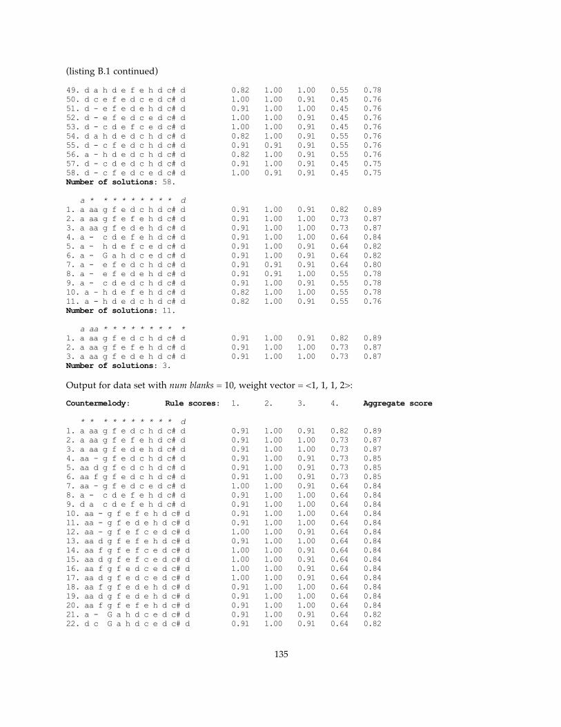
(listing B.1 continued)

49. d a h d e f e h d c# d 0.82 1.00 1.00 0.55 0.7850. d c e f e d c e d c# d 1.00 1.00 0.91 0.45 0.7651. d - e f e d e h d c# d 0.91 1.00 1.00 0.45 0.7652. d - e f e d c e d c# d 1.00 1.00 0.91 0.45 0.7653. d - c d e f c e d c# d 1.00 1.00 0.91 0.45 0.7654. d a h d e d c h d c# d 0.82 1.00 0.91 0.55 0.7655. d - c f e d c h d c# d 0.91 0.91 0.91 0.55 0.7656. a - h d e d c h d c# d 0.82 1.00 0.91 0.55 0.7657. d - c d e d c h d c# d 0.91 1.00 0.91 0.45 0.7558. d - c f e d c e d c# d 1.00 0.91 0.91 0.45 0.75Number of solutions: 58.

a * * * * * * * * * d1. a aa g f e d c h d c# d 0.91 1.00 0.91 0.82 0.892. a aa g f e f e h d c# d 0.91 1.00 1.00 0.73 0.873. a aa g f e d e h d c# d 0.91 1.00 1.00 0.73 0.874. a - c d e f e h d c# d 0.91 1.00 1.00 0.64 0.845. a - h d e f c e d c# d 0.91 1.00 0.91 0.64 0.826. a - G a h d c e d c# d 0.91 1.00 0.91 0.64 0.827. a - e f e d c h d c# d 0.91 0.91 0.91 0.64 0.808. a - e f e d e h d c# d 0.91 0.91 1.00 0.55 0.789. a - c d e d c h d c# d 0.91 1.00 0.91 0.55 0.7810. a - h d e f e h d c# d 0.82 1.00 1.00 0.55 0.7811. a - h d e d c h d c# d 0.82 1.00 0.91 0.55 0.76Number of solutions: 11.

a aa * * * * * * * * *1. a aa g f e d c h d c# d 0.91 1.00 0.91 0.82 0.892. a aa g f e f e h d c# d 0.91 1.00 1.00 0.73 0.873. a aa g f e d e h d c# d 0.91 1.00 1.00 0.73 0.87Number of solutions: 3.

Output for data set with num blanks = 10, weight vector = <1, 1, 1, 2>:

Countermelody: Rule scores: 1. 2. 3. 4. Aggregate score

* * * * * * * * * * d1. a aa g f e d c h d c# d 0.91 1.00 0.91 0.82 0.892. a aa g f e f e h d c# d 0.91 1.00 1.00 0.73 0.873. a aa g f e d e h d c# d 0.91 1.00 1.00 0.73 0.874. aa - g f e d c h d c# d 0.91 1.00 0.91 0.73 0.855. aa d g f e d c h d c# d 0.91 1.00 0.91 0.73 0.856. aa f g f e d c h d c# d 0.91 1.00 0.91 0.73 0.857. aa - g f e d c e d c# d 1.00 1.00 0.91 0.64 0.848. a - c d e f e h d c# d 0.91 1.00 1.00 0.64 0.849. d a c d e f e h d c# d 0.91 1.00 1.00 0.64 0.8410. aa - g f e f e h d c# d 0.91 1.00 1.00 0.64 0.8411. aa - g f e d e h d c# d 0.91 1.00 1.00 0.64 0.8412. aa - g f e f c e d c# d 1.00 1.00 0.91 0.64 0.8413. aa d g f e f e h d c# d 0.91 1.00 1.00 0.64 0.8414. aa f g f e f c e d c# d 1.00 1.00 0.91 0.64 0.8415. aa d g f e f c e d c# d 1.00 1.00 0.91 0.64 0.8416. aa f g f e d c e d c# d 1.00 1.00 0.91 0.64 0.8417. aa d g f e d c e d c# d 1.00 1.00 0.91 0.64 0.8418. aa f g f e d e h d c# d 0.91 1.00 1.00 0.64 0.8419. aa d g f e d e h d c# d 0.91 1.00 1.00 0.64 0.8420. aa f g f e f e h d c# d 0.91 1.00 1.00 0.64 0.8421. a - G a h d c e d c# d 0.91 1.00 0.91 0.64 0.8222. d c G a h d c e d c# d 0.91 1.00 0.91 0.64 0.82

135

(listing B.1 continued)

23. d a G a h d c e d c# d 0.91 1.00 0.91 0.64 0.8224. a - h d e f c e d c# d 0.91 1.00 0.91 0.64 0.8225. d c g f e d e h d c# d 0.91 0.91 1.00 0.64 0.8226. d - G a h d c e d c# d 0.91 1.00 0.91 0.64 0.8227. d c g f e f e h d c# d 0.91 0.91 1.00 0.64 0.8228. d a h d e f c e d c# d 0.91 1.00 0.91 0.64 0.8229. d - g f e d c h d c# d 0.91 1.00 0.91 0.64 0.8230. d a e f e d c h d c# d 0.91 0.91 0.91 0.64 0.8031. d c g f e d c h d c# d 0.91 0.91 0.91 0.64 0.8032. a - e f e d c h d c# d 0.91 0.91 0.91 0.64 0.8033. d - g f e d e h d c# d 0.91 1.00 1.00 0.55 0.8034. d c e f e d e h d c# d 0.91 1.00 1.00 0.55 0.8035. d - g f e f c e d c# d 1.00 1.00 0.91 0.55 0.8036. d - g f e f e h d c# d 0.91 1.00 1.00 0.55 0.8037. d - c d e f e h d c# d 0.91 1.00 1.00 0.55 0.8038. d - g f e d c e d c# d 1.00 1.00 0.91 0.55 0.8039. d a e f e d e h d c# d 0.91 0.91 1.00 0.55 0.7840. a - e f e d e h d c# d 0.91 0.91 1.00 0.55 0.7841. d - c f e d e h d c# d 0.91 0.91 1.00 0.55 0.7842. d c g f e d c e d c# d 1.00 0.91 0.91 0.55 0.7843. d c g f e f c e d c# d 1.00 0.91 0.91 0.55 0.7844. d a c d e d c h d c# d 0.91 1.00 0.91 0.55 0.7845. a - c d e d c h d c# d 0.91 1.00 0.91 0.55 0.7846. d - e f e d c h d c# d 0.91 1.00 0.91 0.55 0.7847. d c e f e d c h d c# d 0.91 1.00 0.91 0.55 0.7848. a - h d e f e h d c# d 0.82 1.00 1.00 0.55 0.7849. d a h d e f e h d c# d 0.82 1.00 1.00 0.55 0.7850. d c e f e d c e d c# d 1.00 1.00 0.91 0.45 0.7651. d - e f e d e h d c# d 0.91 1.00 1.00 0.45 0.7652. d - e f e d c e d c# d 1.00 1.00 0.91 0.45 0.7653. d - c d e f c e d c# d 1.00 1.00 0.91 0.45 0.7654. d a h d e d c h d c# d 0.82 1.00 0.91 0.55 0.7655. d - c f e d c h d c# d 0.91 0.91 0.91 0.55 0.7656. a - h d e d c h d c# d 0.82 1.00 0.91 0.55 0.7657. d - c d e d c h d c# d 0.91 1.00 0.91 0.45 0.7558. d - c f e d c e d c# d 1.00 0.91 0.91 0.45 0.75Number of solutions: 58.

a * * * * * * * * * *1. a aa g f e d c h d c# d 0.91 1.00 0.91 0.82 0.892. a - G F E D A B D C# d 0.91 1.00 1.00 0.73 0.873. a D G F E D A B D C# d 0.91 1.00 1.00 0.73 0.874. a aa g f e f e h d c# d 0.91 1.00 1.00 0.73 0.875. a aa g f e d e h d c# d 0.91 1.00 1.00 0.73 0.876. a - G F E D C B D C# d 0.91 1.00 0.91 0.73 0.857. a D G F E D C B D C# d 0.91 1.00 0.91 0.73 0.858. a - G F C D C E D C# d 1.00 1.00 0.91 0.64 0.849. a - c d e f e h d c# d 0.91 1.00 1.00 0.64 0.8410. a - G F E D C E D C# d 1.00 1.00 0.91 0.64 0.8411. a D G F C D C E D C# d 1.00 1.00 0.91 0.64 0.8412. a D G F E D C E D C# d 1.00 1.00 0.91 0.64 0.8413. a - h d e f c e d c# d 0.91 1.00 0.91 0.64 0.8214. a - G a h d c e d c# d 0.91 1.00 0.91 0.64 0.8215. a - e f e d c h d c# d 0.91 0.91 0.91 0.64 0.8016. a - e f e d e h d c# d 0.91 0.91 1.00 0.55 0.7817. a - c d e d c h d c# d 0.91 1.00 0.91 0.55 0.7818. a - h d e f e h d c# d 0.82 1.00 1.00 0.55 0.7819. a - h d e d c h d c# d 0.82 1.00 0.91 0.55 0.76Number of solutions: 19.

136

(listing B.1 continued)

Output for data set with num blanks = 11, weight vector = <1, 1, 1, 2>:

Countermelody: Rule scores: 1. 2. 3. 4. Aggregate score

* * * * * * * * * * *1. a aa g f e d c h d c# d 0.91 1.00 0.91 0.82 0.892. a - G F E D A B D C# d 0.91 1.00 1.00 0.73 0.873. a D G F E D A B D C# d 0.91 1.00 1.00 0.73 0.874. a aa g f e f e h d c# d 0.91 1.00 1.00 0.73 0.875. a aa g f e d e h d c# d 0.91 1.00 1.00 0.73 0.876. D Bb C F E D A B D C# d 0.91 0.91 1.00 0.73 0.857. a - G F E D C B D C# d 0.91 1.00 0.91 0.73 0.858. aa - g f e d c h d c# d 0.91 1.00 0.91 0.73 0.859. aa f g f e d c h d c# d 0.91 1.00 0.91 0.73 0.8510. aa d g f e d c h d c# d 0.91 1.00 0.91 0.73 0.8511. a D G F E D C B D C# d 0.91 1.00 0.91 0.73 0.8512. aa - g f e d e h d c# d 0.91 1.00 1.00 0.64 0.8413. D - G F E D A B D C# d 0.91 1.00 1.00 0.64 0.8414. a - c d e f e h d c# d 0.91 1.00 1.00 0.64 0.8415. a - G F E D C E D C# d 1.00 1.00 0.91 0.64 0.8416. a - G F C D C E D C# d 1.00 1.00 0.91 0.64 0.8417. aa - g f e f e h d c# d 0.91 1.00 1.00 0.64 0.8418. d a c d e f e h d c# d 0.91 1.00 1.00 0.64 0.8419. aa - g f e f c e d c# d 1.00 1.00 0.91 0.64 0.8420. aa - g f e d c e d c# d 1.00 1.00 0.91 0.64 0.8421. aa d g f e d c e d c# d 1.00 1.00 0.91 0.64 0.8422. a D G F C D C E D C# d 1.00 1.00 0.91 0.64 0.8423. a D G F E D C E D C# d 1.00 1.00 0.91 0.64 0.8424. aa d g f e d e h d c# d 0.91 1.00 1.00 0.64 0.8425. aa f g f e f c e d c# d 1.00 1.00 0.91 0.64 0.8426. aa d g f e f c e d c# d 1.00 1.00 0.91 0.64 0.8427. aa f g f e f e h d c# d 0.91 1.00 1.00 0.64 0.8428. aa d g f e f e h d c# d 0.91 1.00 1.00 0.64 0.8429. aa f g f e d e h d c# d 0.91 1.00 1.00 0.64 0.8430. aa f g f e d c e d c# d 1.00 1.00 0.91 0.64 0.8431. D - C F E D A B D C# d 0.91 0.91 1.00 0.64 0.8232. d - G a h d c e d c# d 0.91 1.00 0.91 0.64 0.8233. a - h d e f c e d c# d 0.91 1.00 0.91 0.64 0.8234. d a G a h d c e d c# d 0.91 1.00 0.91 0.64 0.8235. d c G a h d c e d c# d 0.91 1.00 0.91 0.64 0.8236. d a h d e f c e d c# d 0.91 1.00 0.91 0.64 0.8237. a - G a h d c e d c# d 0.91 1.00 0.91 0.64 0.8238. d c g f e d e h d c# d 0.91 0.91 1.00 0.64 0.8239. d c g f e f e h d c# d 0.91 0.91 1.00 0.64 0.8240. d - g f e d c h d c# d 0.91 1.00 0.91 0.64 0.8241. D - A F E D C B D C# d 0.91 1.00 0.91 0.64 0.8242. D - G F E D C B D C# d 0.91 1.00 0.91 0.64 0.8243. d a e f e d c h d c# d 0.91 0.91 0.91 0.64 0.8044. a - e f e d c h d c# d 0.91 0.91 0.91 0.64 0.8045. d c g f e d c h d c# d 0.91 0.91 0.91 0.64 0.8046. D - G F C D C E D C# d 1.00 1.00 0.91 0.55 0.8047. D - G F E D C E D C# d 1.00 1.00 0.91 0.55 0.8048. D - A F E D A B D C# d 0.91 1.00 1.00 0.55 0.8049. d - g f e d e h d c# d 0.91 1.00 1.00 0.55 0.8050. d - c d e f e h d c# d 0.91 1.00 1.00 0.55 0.8051. d - g f e f e h d c# d 0.91 1.00 1.00 0.55 0.8052. d - g f e f c e d c# d 1.00 1.00 0.91 0.55 0.8053. d c e f e d e h d c# d 0.91 1.00 1.00 0.55 0.8054. d - g f e d c e d c# d 1.00 1.00 0.91 0.55 0.80

137

(listing B.1 continued)

55. d - c f e d e h d c# d 0.91 0.91 1.00 0.55 0.7856. d c g f e f c e d c# d 1.00 0.91 0.91 0.55 0.7857. a - e f e d e h d c# d 0.91 0.91 1.00 0.55 0.7858. d c g f e d c e d c# d 1.00 0.91 0.91 0.55 0.7859. d a e f e d e h d c# d 0.91 0.91 1.00 0.55 0.7860. a - c d e d c h d c# d 0.91 1.00 0.91 0.55 0.7861. d c e f e d c h d c# d 0.91 1.00 0.91 0.55 0.7862. d a c d e d c h d c# d 0.91 1.00 0.91 0.55 0.7863. d - e f e d c h d c# d 0.91 1.00 0.91 0.55 0.7864. a - h d e f e h d c# d 0.82 1.00 1.00 0.55 0.7865. d a h d e f e h d c# d 0.82 1.00 1.00 0.55 0.7866. d - c d e f c e d c# d 1.00 1.00 0.91 0.45 0.7667. d - e f e d c e d c# d 1.00 1.00 0.91 0.45 0.7668. d - e f e d e h d c# d 0.91 1.00 1.00 0.45 0.7669. d c e f e d c e d c# d 1.00 1.00 0.91 0.45 0.7670. d a h d e d c h d c# d 0.82 1.00 0.91 0.55 0.7671. a - h d e d c h d c# d 0.82 1.00 0.91 0.55 0.7672. D - C F E D C B D C# d 0.91 0.91 0.91 0.55 0.7673. d - c f e d c h d c# d 0.91 0.91 0.91 0.55 0.7674. d - c d e d c h d c# d 0.91 1.00 0.91 0.45 0.7575. D - C F E D C E D C# d 1.00 0.91 0.91 0.45 0.7576. d - c f e d c e d c# d 1.00 0.91 0.91 0.45 0.75Number of solutions: 76.

138

APPENDIX C. COUNTERPOINTS IN ARTIFICIAL NEURAL NETWORK TRAINING

We show here the data and configurations used in neural network training (chapter 5, section 5.2):

C.1. The 100 training and validation exemplars.

C.2. The above data reconfigured as partially filled countermelodies for the training of networks to

produce non-increasing scores with respect to partial countermelody lengths.

C.3. Comparisons between the expert’s and the neural network’s outputs on the validation exemplars,

within various grading schemes.

C.1. The 100 Training and Validation Exemplars

In training the artificial neural network to compute a function of rule scores, we used 100 counterpoints.

Using the Palestrina program, we first generated ten distinct cantus firmi, two for each of five modes,

ending on the notes D, E, F, G, and a, respectively. For each of the cantus firmi, we further generated ten

grammatically correct countermelodies in first species. All the melodies had a length of ten notes.

Listing C.1 groups the countermelodies by their respective modes (dorian, phrygian, lydian,

mixolydian, and aeolian), and presents the original evaluations by the expert.

Listing C.1. Training and validation exemplars

TRAINING DATA

Dorian mode

Counterpoint Expert evaluation

d d c d e f e d c# d D F E D C# D E F E D 0.72

d d g f e d c d c# d D F E D C# D E F E D 0.5

d d c d e d c d c# d D F E D C# D E F E D 0.4

d d e f e h c d c# d D F E D C# D E F E D 0.55

d d g f e h c d c# d D F E D C# D E F E D 0.55

D D E A Bb A B D C# D D a G F G a G F E D 0.4

139

(listing C.1 continued)

D C B A B C E D C# D D a G F G a G F E D 0.65

D C E D B C B D C# D D a G F G a G F E D 0.5

D C Bb A B C E D C# D D a G F G a G F E D 0.5

D D E D C A B D C# D D a G F G a G F E D 0.67

d d g f e f e d c# d D F E D C# D E F E D 0.7

D D G F E B C D C# D D F E D C# D E F E D 0.4

d c g f e d c d c# d D F E D C# D E F E D 0.5

D D E A B A B D C# D D a G F G a G F E D 0.3

D D E D B C B D C# D D a G F G a G F E D 0.45

D D GG A B C E D C# D D a G F G a G F E D 0.5

Phrygian mode

Counterpoint Expert evaluation

e d e c d e f e d e E F G a h G a G F E 0.97

e d e c d g f e d e E F G a h G a G F E 0.75

E D E C D E F C D E E F G a h G a G F E 0.45

e d h c d g f e d e E F G a h G a G F E 0.7

E D E F G d c h a h E F G a h G a G F E 0.5

e d e hh aa g f e d e E F G G a h a G F E 0.4

140

(listing C.1 continued)

h a h E F G c h a h E F G G a h a G F E 0.65

e a h d c d c h a h E F G G a h a G F E 0.45

h a e d c d c h a h E F G G a h a G F E 0.32

e d e d c d f e d e E F G G a h a G F E 0.8E D E C D E F E D E E F G a h G a G F E 0.69

e a h c d g f e d e E F G a h G a G F E 0.8

E A B C B C F E D E E F G a h G a G F E 0.5

h a h d c d f e d e E F G G a h a G F E 0.77

e d e h c d f e d e E F G G a h a G F E 0.82

E D E B C D F E D E E F G G a h a G F E 0.65

Lydian mode

Counterpoint Expert evaluation

f e d f e d e f g f F c b a G G C D E F 0.6

f e d f e d e aa g f F c b a G G C D E F 0.6

FF FF GG A C B A FF GG FF F c b a G G C D E F 0.45

f e g f g d e aa g f F c b a G G C D E F 0.57

FF FF GG FF C B A FF GG FF F c b a G G C D E F 0.5

c d e f g cc hh aa g f c F G a b a G F E F 0.47

g aa hh aa g cc hh aa g f c F G a b a G F E F 0.3

141

(listing C.1 continued)

c f e c d f e f g f c F G a b a G F E F 0.62

g cc hh aa g f e aa g f c F G a b a G F E F 0.5

g aa hh aa g aa e f g f c F G a b a G F E F 0.28

F E D C B GG A FF GG FF F c b a G G C D E F 0.3

f e d c e d e aa g f F c b a G G C D E F 0.55

f e d c e d e f g f F c b a G G C D E F 0.6

c d h c d f e f g f c F G a b a G F E F 0.55

g f e f g f e aa g f c F G a b a G F E F 0.75

g cc hh aa g aa e f g f c F G a b a G F E F 0.45

Mixolydian mode

Counterpoint Expert evaluation

g aa ee dd cc hh aa g f# g G d c h a G a h a G 0.85

g f e d e h c d c# d G d c h a G a h a G 0.45

g f aa g f e c d c# d G d c h a G a h a G 0.45

g f g d e hh aa g f# g G d c h a G a h a G 0.45

GG GG A D C B A GG FF# GG G d c h a G a h a G 0.8

D E D E D F E F a G d c h c h a h a F# G 0.57

d e d e d e g f aa g d c h c h a h a F# G 0.38

142

(listing C.1 continued)

d e hh aa d e g f aa g d c h c h a h a F# G 0.35

D E D E G F E F a G d c h c h a h a F# G 0.65

D E D C D F E F a G d c h c h a h a F# G 0.55

GG GG A GG C B A GG FF# GG G d c h a G a h a G 0.67

g f aa g cc hh aa g f# g G d c h a G a h a G 0.55

G F a G F E F E F# G G d c h a G a h a G 0.5

d e d e g f g f aa g d c h c h a h a F# G 0.45

aa aa hh aa g aa g f aa g d c h c h a h a F# G 0.25

d e hh aa g aa g f aa g d c h c h a h a F# G 0.3

Aeolian mode

Counterpoint Expert evaluation

aa d e f g aa g aa hh aa a h c a h a E F# G# a 0.62

A GG FF A GG D C A B A a h c a h a E F# G# a 0.6

aa g e f g aa g aa hh aa a h c a h a E F# G# a 0.75

e d e f g aa g aa hh aa a h c a h a E F# G# a 0.52

a G a e d c h a h a a h c a h a E F# G# a 0.42

a G h a G c h a h a a e d c h a E F# G# a 0.85

aa g f aa g cc hh aa hh aa a e d c h a E F# G# a 0.5

143

(listing C.1 continued)

A A B A GG D C A B A a e d c h a E F# G# a 0.45

aa g hh aa hh cc hh aa hh aa a e d c h a E F# G# a 0.7

e a h a d c h a h a a e d c h a E F# G# a 0.67

A GG A C B D C A B A a h c a h a E F# G# a 0.92

e d e f g cc hh aa hh aa a h c a h a E F# G# a 0.7

a D E F E F G a h a a h c a h a E F# G# a 0.47

a a h a d c h a h a a e d c h a E F# G# a 0.45

aa g hh aa g cc hh aa hh aa a e d c h a E F# G# a 0.45

aa g f aa g aa g aa hh aa a e d c h a E F# G# a 0.6

VALIDATION DATA

Dorian mode

Counterpoint Expert evaluation

D D C F E B C D C# D D F E D C# D E F E D 0.45

d d c h e d c d c# d D F E D C# D E F E D 0.55

D D E A B C B D C# D D a G F G a G F E D 0.65

D A Bb A B C E D C# D D a G F G a G F E D 0.65

Phrygian mode

Counterpoint Expert evaluation

e d h c d e f e d e E F G a h G a G F E 0.77

144

(listing C.1 continued)

E D E D B C F E D E E F G a h G a G F E 0.57

e aa g hh aa g f e d e E F G G a h a G F E 0.6

e a h d c d f e d e E F G G a h a G F E 0.95

Lydian mode

Counterpoint Expert evaluation

FF FF GG C B GG A FF GG FF F c b a G G C D E F 0.35

f e g f e d e aa g f F c b a G G C D E F 0.77

C D E D G F E a G F c F G a b a G F E F 0.52

g aa hh aa dd cc hh aa g f c F G a b a G F E F 0.3

Mixolydian mode

Counterpoint Expert evaluation

G G a G F E F E F# G G d c h a G a h a G 0.58

g f e d c d c d c# d G d c h a G a h a G 0.75

D E G F G F G F a G d c h c h a h a F# G 0.58

D E G F G F E F a G d c h c h a h a F# G 0.6

Aeolian mode

Counterpoint Expert evaluation

aa d e f g cc hh aa hh aa a h c a h a E F# G# a 0.57

aa g e f g cc hh aa hh aa a h c a h a E F# G# a 0.55

145

(listing C.1 continued)

a G h a d c h a h a a e d c h a E F# G# a 0.3

aa g f e d c h a h a a e d c h a E F# G# a 0.9

C.2. Partially Filled Countermelodies to Satisfy the Assumption of the Best-First Algorithm

Listing C.2 shows the mixolydian exemplars reconfigured as partially filled countermelodies for the

training of networks to produce non-increasing scores of partial countermelodies with respect to length.

Expert’s scores are shown as percentages, as 1-of-10 bit vectors (000000001 represents an expert’s score of

0.9 and above, 0000000010 a score between 0.8 and 0.89, etc.), and as 1-of-5 bit vectors (based on the

second grade partition shown in table 5.1: 00001 represents an expert’s scores of 0.8 and above, 00010 a

score between 0.6 and 0.79, 00100 between 0.40 and 0.59, 01000 between 0.2 and 0.39, and 10000 between

0.0 and 0.19). Partial countermelodies receive the same score as their full counterparts; where identical

partial countermelodies have full counterparts with different scores, these partial countermelodies

receive the higher/highest of these different scores, with subsequent duplicate entries removed (e.g.,

see partial countermelodies nos. 41–52 in the training set, and nos. 15–17 in the validation set).

Listing C.2. Partially filled countermelodies for network training to produce non-increasing scores

Cantus firmus: <d, c, h, c, h, a, h, a, F#, G>

Mixolydian mode training data

(Partial) countermelody Expert’s 1-of-10 representation 1-of-5 representationscore of expert’s score of expert’s score

1. D E D E G F E F a G 0.65 0000001000 000102. d e d e g f g f aa g 0.45 0000100000 001003. D E D C D F E F a G 0.55 0000010000 001004. D E D E D F E F a G 0.57 0000010000 001005. d e hh aa g aa g f aa g 0.3 0001000000 010006. aa aa hh aa g aa g f aa g 0.25 0010000000 010007. d e hh aa d e g f aa g 0.35 0001000000 010008. d e d e d e g f aa g 0.38 0001000000 01000

9. – E D E G F E F a G 0.65 0000001000 0001010. – e d e g f g f aa g 0.45 0000100000 0010011. – E D C D F E F a G 0.55 0000010000 0010012. – E D E D F E F a G 0.57 0000010000 0010013. – e hh aa g aa g f aa g 0.3 0001000000 0100014. – aa hh aa g aa g f aa g 0.25 0010000000 01000 15. – e hh aa d e g f aa g 0.35 0001000000 0100016. – e d e d e g f aa g 0.38 0001000000 01000

146

(listing C.2 continued)

17. – – D E G F E F a G 0.65 0000001000 0001018. – – d e g f g f aa g 0.45 0000100000 0010019. – – D C D F E F a G 0.55 0000010000 0010020. – – D E D F E F a G 0.57 0000010000 0010021. – – hh aa g aa g f aa g 0.3 0001000000 0100022. – – hh aa g aa g f aa g 0.25 0010000000 01000 23. – – hh aa d e g f aa g 0.35 0001000000 0100024. – – d e d e g f aa g 0.38 0001000000 01000

25. – – – E G F E F a G 0.65 0000001000 0001026. – – – e g f g f aa g 0.45 0000100000 0010027. – – – C D F E F a G 0.55 0000010000 0010028. – – – E D F E F a G 0.57 0000010000 0010029. – – – aa g aa g f aa g 0.3 0001000000 0100030. – – – aa g aa g f aa g 0.25 0010000000 01000 31. – – – aa d e g f aa g 0.35 0001000000 0100032. – – – e d e g f aa g 0.38 0001000000 01000

33. – – – – G F E F a G 0.65 0000001000 0001034. – – – – g f g f aa g 0.45 0000100000 0010035. – – – – D F E F a G 0.55 0000010000 0010036. – – – – D F E F a G 0.57 0000010000 0010037. – – – – g aa g f aa g 0.3 0001000000 0100038. – – – – g aa g f aa g 0.25 0010000000 01000 39. – – – – d e g f aa g 0.35 0001000000 0100040. – – – – d e g f aa g 0.38 0001000000 01000

41. – – – – – F E F a G 0.65 0000001000 0001042. – – – – – f g f aa g 0.45 0000100000 0010043. – – – – – aa g f aa g 0.3 0001000000 0100044. – – – – – e g f aa g 0.38 0001000000 01000

45. – – – – – – E F a G 0.65 0000001000 0001046. – – – – – – g f aa g 0.45 0000100000 00100

47. – – – – – – – F a G 0.65 0000001000 0001048. – – – – – – – f aa g 0.45 0000100000 00100

49. – – – – – – – – a G 0.65 0000001000 0001050. – – – – – – – – aa g 0.45 0000100000 00100

51. – – – – – – – – – G 0.65 0000001000 0001052. – – – – – – – – – g 0.45 0000100000 00100

Mixolydian mode validation data

(Partial) countermelody Expert’s 1-of-10 representation 1-of-5 representationscore of expert’s score of expert’s score

1. D E G F G F E F a G 0.6 0000001000 000102. D E G F G F G F a G 0.58 0000010000 00100

147

(listing C.2 continued)

3. – E G F G F E F a G 0.6 0000001000 000104. – E G F G F G F a G 0.58 0000010000 00100

5. – – G F G F E F a G 0.6 0000001000 000106. – – G F G F G F a G 0.58 0000010000 00100

7. – – – F G F E F a G 0.6 0000001000 000108. – – – F G F G F a G 0.58 0000010000 00100

9. – – – – G F E F a G 0.6 0000001000 0001010. – – – – G F G F a G 0.58 0000010000 00100

11. – – – – – F E F a G 0.6 0000001000 0001012. – – – – – F G F a G 0.58 0000010000 00100

13. – – – – – – E F a G 0.6 0000001000 0001014. – – – – – – G F a G 0.58 0000010000 00100

15. – – – – – – – F a G 0.6 0000001000 00010

16. – – – – – – – – a G 0.6 0000001000 00010

17. – – – – – – – – – G 0.6 0000001000 00010

148

C.3. Comparisons between the Expert’s and the Neural Network’s Evaluations of the Validation Exemplars, within Various Grading Schemes

We show here the detailed comparisons between the expert’s grading and the neural network’s trained

output, based on the grading schemes described in chapter 5, section 5.2, and illustrated in table 5.1. For

each grading scheme, we compare the grades imposed on each of the twenty validation exemplars.

Section C.3.1 shows the outputs of neural networks with 40 input nodes, and section C.3.2 of networks

with 60 input nodes. The specifications of the networks trained in the respective sections are given in

table C.1 (both specifications are identical except for the number of input nodes).

Table C.1. Specifications of the neural networks trained with various grading schemes. The number of output nodes specified here corresponds to the network trained on the 1-of-5 partitions; the network trained on the pass-fail grading scheme would have 2 output notes, and the network trained on the 1-of-10 grading scheme would have 10 output nodes. Output of networks (a) and (b) are described in sections C.3.1 and C.3.2, respectively.

(a ) (b)network type: back propagation back propagation

with validation and epoch training, with validation and epoch training,nodes with bias term nodes with bias term

learning rate 0.1 0.1momentum term 0.1 0.1error threshold 0.1 0.1no. iterations until error threshold is achieved until error threshold is achieved

or until validation error increases or until validation error increasesno. layers 3 3no. inputs 40 60no. middle layer nodes 8 15no. outputs 5 5layer connections maximal maximal

149

C.3.1. Neural Network with 40 Input Nodes

The 40 input nodes correspond to the errors detected by the four artistry rules, indicated in a 1-of-10

vector: one for each note of the countermelody, whose length is 10. The network architecture of all

networks trained in this section is the one shown in figure 5.2. The following table (C.2) shows the

neural network’s evaluation of the 20 validation exemplars, represented as seven grading schemes

(indicated as “1.” through “7.”) corresponding to those shown in table 5.1. For each grading scheme, the

output reflects the composite evaluations of ten separately trained networks, one for each of the ten

different cantus firmi used in the training and validation sets.

Table C.2. Comparison of expert’s and network’s grades of 20 validation exemplars under various grading schemes (40 input nodes)

1. 2. 3. 4. 5. 6. 7. 8.

ExpANN Exp ANN Exp ANN Exp ANN ExpANN ExpANN Exp ANN Exp ANN

1. F P C C F D D C D C D C D C 0.4 0.52. P P C C D D C D C C C C C C 0.5 0.53. P P B C D D C C B C B B B C 0.6 0.54. P P B C D D C D B C B B B C 0.6 0.55. P P B A C D B D A B A C A A 0.7 0.96. P P C C D D C D C C C B B C 0.5 0.57. P F B C D F C D B D B D B F 0.6 0.68. P P A B A C A C A A A A A A 0.9 0.79. F F D D F F F D F F F D F C 0.3 0.310. P P B C C D B F A C A C A B 0.7 0.511. P P C B D C D F C A C B C A 0.5 0.712. F F D D F F F C F F F B F F 0.3 0.313. P P C C D D C B C C C A B C 0.5 0.514. P F B C C F B B A D A B A C 0.7 0.415. P F C C D F C C C F C C B F 0.5 0.316. P P B B D D C C B C B C B B 0.6 0.517. P P C B D C C C C A C A B A 0.5 0.718. P P C B D C C B C A C A C A 0.5 0.719. F F D B F F F D F A F D F A 0.3 0.420. P P A B A D A D A B A D A B 0.9 0.6

150

C.3.2. Neural Network with 60 Input Nodes

In addition to having 40 input nodes as for the network used in section C.3.1, the networks here consist of

additional input nodes giving information on each of the ten notes of the cantus firmus and of the

countermelody, for a total of 60 input nodes. The network architecture for all networks trained in this

section is the one shown in figure 5.3. As did table C.2, the following table (C.3) shows the evaluations

according to the seven grading schemes shown in table 5.1. For each grading scheme, the output reflects

the evaluations of a single network, trained on all 80 training and 20 validation exemplars.

Table C.3. Comparison of expert’s and network’s grades of 20 validation exemplars under various grading schemes (60 input nodes)

1. 2. 3. 4. 5. 6. 7. 8.

ExpANN Exp ANN Exp ANN Exp ANN ExpANN ExpANN Exp ANN Exp ANN

1. F P C C F D D C D D D C D C 0.4 0.52. P P C C D D C D C C C C C C 0.5 0.53. P P B C D D C D B C B C B C 0.6 0.54. P P B C D D C D B C B C B C 0.6 0.55. P P B B C D B B A A A B A A 0.7 0.56. P P C B D D C D C B C B B B 0.5 0.47. P P B C D D C C B D B B B A 0.6 0.58. P P A C A D A D A C A C A C 0.9 0.59. F P D B F D F C F B F B F A 0.3 0.510. P P B C C D B C A A A C A B 0.7 0.511. P P C B D D D C C C C C C B 0.5 0.412. F F D C F F F F F C F C F F 0.3 0.413. P P C C D D C D C C C C B C 0.5 0.514. P F B B C F B D A D A B A A 0.7 0.415. P F C C D F C D C F C D B D 0.5 0.516. P F B C D F C C B C B C B B 0.6 0.417. P P C C D F C D C D C D B A 0.5 0.418. P P C B D F C D C A C B C A 0.5 0.419. F F D C F F F D F D F D F D 0.3 0.420. P F A C A F A D A D A D A D 0.9 0.4

151

APPENDIX D. IMPLEMENTATION OF MUSIC COMPOSITION ALGORITHMS

We discuss here the implementation of the two music composition algorithms discussed in the text,

including the exhaustive algorithm (chapter 6, sections 6.1–3). All algorithms are modules of the

overall program we call “Palestrina,” after the great sixteenth-century composer whose style species

counterpoint emulates. We programmed Palestrina in C++ using object-oriented design and

implementation, and show here the key objects and methods used.

D.1. Inheritance Hierarchies and Navigability of the Classes

In this section, we outline also inheritance hierarchies and describe the navigability between the main

classes in the Palestrina application. We have omitted a considerable amount of detail and have

shown only what is relevant to the discussion in the main text.

D.1.1. General Interactions

The main classes in the Palestrina program are the following (base classes):

CApplication, CAnalyzer, CRulesManager, CRules, CBaseSearchEngine. In the following, whenever a

base class is referenced, the reader is asked to add the phrase “and its subclasses …” where

appropriate. The CApplication class and its subclasses provide the external interface. These

application classes invoke the CAnalyzer class to convert external data into internal form and set up

the required data structures. The CAnalyzer calls in turn the various algorithms to generate and

diagnose countermelodies (fig. D.1).

CPalestrinaComposerApp

C12OptBestFirstSEApp

…

CAnalyzer

COptimizedBestFirstSearchEngine

…

C12OptFillBlanksBestFirstSEApp CFillBlanks12Analyzer

… …

Fig. D.1. Navigability between the application and analyzer classes

The CAnalyzer directly runs the generate-and-test algorithm, and uses CBaseSearchEngine to run the

best-first search algorithm and to interface with the genetic algorithm classes (fig. D.2).

152

CAnalyzer CBaseSearchEngine

CGeneticAlgorithmAnalyzer12 CGeneticAlgorithmSearchEngine12 CGADriverInterface12

CGADriverInterfaceCGeneticAlgorithmSearchEngine

…

…

CGADriverInterface12

CPalGA<…>

t_AbstractGA<…>

CPalGA12

CGADriverInterface

… …

Fig. D.2. Navigability between the analyzer, search engine, and genetic algorithm classes

Both the analyzer and search engine classes rely on the CRulesManager to obtain the various CRules’s

responses to the various countermelodies submitted for approval (fig. D.3).

COptimizedSearchEngine

CAnalyzer

C12OBSSearchEngineAnalyzer

…

CBaseSearchEngine

COptimizedBestFirstSearchEngine

…

CFillBlanks12Analyzer COptimizedBestFirstFillBlanksSearchEngine

…

C12RulesManager

Fig. D.3. Navigability between analyzer, search engine, and rules manager classes

Further details of the class hierarchies are quite complex: here we shall only attempt to

describe other classes used by the classes mentioned in the main text and in the subsequent sections

(CAnalyzer, COptimizedSearchEngine, COptimizedBestFirstSearchEngine,

COptimizdBestFirstFillBlanksSearchEngine, and t_CAbstractGA).

153

D.1.2. Best-First Search Engine and Genetic Algorithm Classes

The best-first search engine class implements the best-first search algorithm using the priority queue

and a dynamic list to retain information on the partial countermelodies in the process of conducting the

search. Figure D.4 shows the classes used by the best-first search engine class.

COptimizedSearchEngine

…

CBaseSearchEngine

COptimizedBestFirstSearchEngine

CChainedList*

CChainedListNode

CChainedListNode

CChainedListNodeCNoteInterval

CNoteInterval

CNoteInterval

CChainedListNode

CNoteInterval

optimizedNodeInfo optimizedNodeInfo..

priority_queue

optimizedNodeInfo

...

COptimizedBestFirstFillBlanksSearchEngine

Fig. D.4. Classes used by the best-first search engine class

The genetic algorithm controls a population class that in turn maintains a population of

hypotheses, consisting of chromosomes composed of genes. The population class also regenerates itself

at each iteration of the algorithm with the probabilistic assistance of a roulette wheel class. Figure

D.5 shows the objects used by the genetic algorithm class:

CPalGA<…>

t_AbstractGA<…>

CPalGAXY

…

t_AbstractPopulationType<…>

CBasePalPop<…>

…

t_AbstractRouletteWheel<…>

CRouletteWheel<…> orCScaledRouletteWheel<…>

t_ChromosomeType<…>

t_CHypothesis<…>

t_GeneType<…>

Fig. D.5. Classes used by the genetic algorithm class

154

D.1.3. Interactions with the Backpropagation Artificial Neural Network

One choice of evaluation function for the best-first search and genetic algorithms is the output of a

trained neural network. We made the connection with the neural network through the rules manager

class, which communicates with the neural network through a driver class (see below). The best-first

search classes then call upon the rules manager to evaluate candidate countermelodies, while the

genetic algorithm classes invoke the rules manager indirectly through the analyzer (figs. D.6–7).

COptimizedSearchEngine

CAnalyzer

C12OBSSearchEngineNeuralnetAnalyzer

…

CBaseSearchEngine

CNeuralNetOptimizedBestFirstSearchEngine

…

C12NeuralNetRulesManager

CNeuralNetEngine CHitVector

Fig. D.6. Navigability between the neural network based analyzer, best-first search engine, and rules manager classes. Compare figure D.7.

CGeneticAlgorithmNeuralNetAnalyzer12(t_ga5.h)

C12NeuralNetRulesManager(CNeuralNetRulesManagers.h)

CGeneticAlgorithmSearchEngine12(t_ga5.h)

CGeneticAlgorithmAnalyzer12(t_ga5.h)

CNeuralNetAnalyzer(CNeuralNetAnalyzers.h)

CGADriverInterface12(t_gaDriverInterface.h)

CPalGA12(t_PopBasedPalGA.h)

Fig. D.7. Navigability between the neural network based analyzer, genetic algorithm search engine, and rules manager classes.

155

Note that in both figures D.6 and 7, it is the neural net rules manager that communicates with the

neural network, through CBPWithValidationEpochBiasedFunction, a driver class that acts as a go-

between for the neural network (fig. D.8).

C12NeuralNetRulesManager CBPWithValidationEpochBiasedFunction

CBiasedEpochBackpropNetwork

CNeuralNetInterfaceC12RulesManager

…

CBPDriver

…

CAdalineNetwork

Fig. D.8. Interface between the neural net rules manager and the neural network

D.2. Source Code for Generate-and-Test, Best-First Search, and Fill-in-the-Blanks Algorithms

We next present class methods used by the various classes (described above) to implement the key

algorithms used in this dissertation: Generate-and-Test, Best-First Search with Branch-and-Bound

Pruning, and the Fill-in-the-Blanks algorithms. As with the design descriptions in the above sections,

we have confined ourselves to the higher level methods, and have omitted lower level details.

D.2.1. Generate-and-Test

For the psuedocode of this algorithm, see algorithm 6.1. The algorithm to generate and test candidate

melodies is a method in CAnalyzer (algorithm D.1).

void CAnalyzer::GenerateAndTest (void) { short curLevel;fuzzyBoolean result;short initVal = 0;vector <short> index (fNumCantusFirmusNotes, initVal);curLevel = 0;while (curLevel >= 0) {

AddToLists (fNoteArray.at (index.at (curLevel)));result = fRulesManager->AnalyzeData ();if ((result == kError) || (curLevel == (fNumCantusFirmusNotes - 1))) {

if (result != kError)PrintGoodMelody ();

RemoveLastItemFromLists ();while ((curLevel >= 0) && (index.at (curLevel) == fUpperSearchLimitIndex)) {

if (curLevel > 0)RemoveLastItemFromLists ();

index.at (curLevel) = 0;--curLevel;

}if (curLevel >= 0)

index.at (curLevel) = index.at (curLevel) + 1;} // if ((result == kError) || (...))

156

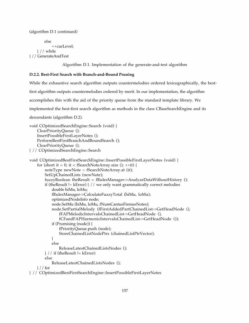
(algorithm D.1 continued)

else ++curLevel;

} // while} // GenerateAndTest

Algorithm D.1. Implementation of the generate-and-test algorithm

D.2.2. Best-First Search with Branch-and-Bound Pruning

While the exhaustive search algorithm outputs countermelodies ordered lexicographically, the best-

first algorithm outputs countermelodies ordered by merit. In our implementation, the algorithm

accomplishes this with the aid of the priority queue from the standard template library. We

implemented the best-first search algorithm as methods in the class CBaseSearchEngine and its

descendants (algorithm D.2).

void COptimizedSearchEngine::Search (void) { ClearPriorityQueue ();InsertPossibleFirstLayerNotes (); PerformBestFirstBranchAndBoundSearch ();ClearPriorityQueue ();

} // COptimizedSearchEngine::Search

void COptimizedBestFirstSearchEngine::InsertPossibleFirstLayerNotes (void) {for (short it = 0; it < fSearchNoteArray.size (); ++it) {

noteType newNote = fSearchNoteArray.at (it);SetUpChainedLists (newNote); fuzzyBoolean theResult = fRulesManager->AnalyzeDataWithoutHistory ();if (theResult != kError) { // we only want grammatically correct melodies

double hiMu, loMu;fRulesManager->CalculateFuzzyTotal (hiMu, loMu);optimizedNodeInfo node;node.SetMu (hiMu, loMu, fNumCantusFirmusNotes);node.SetPartialMelody (fFirstAddedPartChainedList->GetHeadNode (),

fFAPMelodicIntervalsChainedList->GetHeadNode (),fCFandFAPHarmonicIntervalsChainedList->GetHeadNode ());

if (Promising (node)) {fPriorityQueue.push (node);StoreChainedListNodePtrs (chainedListPtrVector);

}else

ReleaseLatestChainedListsNodes (); } // if (theResult != kError)else

ReleaseLatestChainedListsNodes ();} // for

} // COptimizedBestFirstSearchEngine::InsertPossibleFirstLayerNotes

157

(algorithm D.2 continued)

void COptimizedBestFirstSearchEngine::PerformBestFirstBranchAndBoundSearch (void) {fNumMelodiesFound = 0;fTiePossible = true; // used to allow tied melodies to be includedfPrevMu = 0;fGoOn = true;while (! fPriorityQueue.empty () && fGoOn) {

optimizedNodeInfo parent;parent = fPriorityQueue.top ();fPriorityQueue.pop ();if (Leaf (parent))

ProcessLeaf (parent);else

ProcessInternalNode (parent);} // whileDeleteChainedListNodePtrs (chainedListPtrVector);

} // COptimizedBestFirstSearchEngine::PerformBestFirstBranchAndBoundSearch

void COptimizedBestFirstSearchEngine::ProcessLeaf (const optimizedNodeInfo& leafNode) { ++fNumMelodiesFound;AnalyzeCompleteMelody (leafNode); double curMu;leafNode.GetMu (curMu);if (curMu >= fAlphaCut) {

if (fNumMelodiesFound <= fNumMelodiesRequired)PrintGoodMelody ();

elseif (Equal (curMu, fPrevMu))

PrintGoodMelody (); else

fGoOn = false;} // if curMu >= fAlphaCutelse

fGoOn = false;fPrevMu = curMu;

} // COptimizedBestFirstSearchEngine::ProcessLeaf

void COptimizedBestFirstSearchEngine::ProcessInternalNode (const optimizedNodeInfo& parent) {for (short it = 0; it < fSearchNoteArray.size (); ++it) {

noteType newNote = fSearchNoteArray.at (it);SetUpPartialChainedLists (parent, newNote); fuzzyBoolean theResult = fRulesManager->AnalyzeDataWithoutHistory ();if (theResult != kError) {

double hiMu, loMu;fRulesManager->CalculateFuzzyTotal (hiMu, loMu);optimizedNodeInfo child;child = parent;child.SetLevel (parent.GetLevel () + 1);child.SetMu (hiMu, loMu, fNumCantusFirmusNotes); child.SetPartialMelody (fFirstAddedPartChainedList->GetHeadNode (),

158

(algorithm D.2 continued)

fFAPMelodicIntervalsChainedList->GetHeadNode (),fCFandFAPHarmonicIntervalsChainedList->GetHeadNode ());

if (Promising (child)) {fPriorityQueue.push (child);StoreChainedListNodePtrs (chainedListPtrVector);

} // if (Promising (child))else

ReleaseLatestChainedListsNodes ();} // if (theResult != kError)else

ReleaseLatestChainedListsNodes ();} // for it

} // COptimizedBestFirstSearchEngine::ProcessInternalNode

Algorithm D.2. Implementation of the best-first branch-and-bound algorithm

D.2.3. Fill-in-the-Blanks Algorithm Used in the Jeppesen Experiment

The implementation of the algorithm to find alternative solutions at various points in the

countermelody, indicated by blanks, uses the best-first algorithm to generation these alternatives. We

created COptimizedBestFirstFillBlanksSearchEngine, a subclass of the class that handled the best-

first search (see above), COptimizedBestFirstSearchEngine. Only two protected methods had to be

overridden for this subclass: InsertPossibleFirstLayerNotes and ProcessInternalNode (algorithm D.3).

For the description of the Jeppesen Experiment that uses this algorithm, see chapter 5, section 5.1.

void COptimizedBestFirstFillBlanksSearchEngine::InsertPossibleFirstLayerNotes (void) {noteType noteSpecified;if ((noteSpecified = ((CNote *) (fGivenFirstAddedPartList->GetNthItem (1)))->GetNoteType ())

!= unknownNote) { // not a wildcard noteSetUpChainedLists (noteSpecified); fuzzyBoolean theResult = fRulesManager->AnalyzeDataWithoutHistory ();if (theResult != kError) { // we only want grammatically correct melodies

double hiMu, loMu;fRulesManager->CalculateFuzzyTotal (hiMu, loMu);optimizedNodeInfo node;node.SetMu (hiMu, loMu, fNumCantusFirmusNotes);node.SetPartialMelody (fFirstAddedPartChainedList->GetHeadNode (),

fFAPMelodicIntervalsChainedList->GetHeadNode (),fCFandFAPHarmonicIntervalsChainedList->GetHeadNode ());

if (Promising (node)) {fPriorityQueue.push (node);StoreChainedListNodePtrs (chainedListPtrVector);

}else

ReleaseLatestChainedListsNodes (); } // if

159

(algorithm D.3 continued)

else ReleaseLatestChainedListsNodes ();

} // if not a wildcard noteelse { // wildcard note

for (short it = 0; it < fSearchNoteArray.size (); ++it) {noteType newNote = fSearchNoteArray.at (it);SetUpChainedLists (newNote); fuzzyBoolean theResult = fRulesManager->AnalyzeDataWithoutHistory ();if (theResult != kError) { // we only want grammatically correct melodies

double hiMu, loMu;fRulesManager->CalculateFuzzyTotal (hiMu, loMu);optimizedNodeInfo node;node.SetMu (hiMu, loMu, fNumCantusFirmusNotes);node.SetPartialMelody (fFirstAddedPartChainedList->GetHeadNode (),

fFAPMelodicIntervalsChainedList->GetHeadNode (),fCFandFAPHarmonicIntervalsChainedList->GetHeadNode ());

if (Promising (node)) {fPriorityQueue.push (node);StoreChainedListNodePtrs (chainedListPtrVector);

}else

ReleaseLatestChainedListsNodes (); } // ifelse

ReleaseLatestChainedListsNodes ();} // for

} // else wildcard note} // COptimizedBestFirstFillBlanksSearchEngine::InsertPossibleFirstLayerNotes

void COptimizedBestFirstFillBlanksSearchEngine::ProcessInternalNode (const optimizedNodeInfo& parent) {

noteType nextNoteSpecified;if ((nextNoteSpecified = ((CNote *)

(fGivenFirstAddedPartList->GetNthItem (parent.GetLevel () + 1)))->GetNoteType ()) != unknownNote) { // not a wildcard noteSetUpPartialChainedLists (parent, nextNoteSpecified); fuzzyBoolean theResult = fRulesManager->AnalyzeDataWithoutHistory ();if (theResult != kError) {

double hiMu, loMu;fRulesManager->CalculateFuzzyTotal (hiMu, loMu);optimizedNodeInfo child;child = parent;child.SetLevel (parent.GetLevel () + 1);child.SetMu (hiMu, loMu, fNumCantusFirmusNotes); child.SetPartialMelody (fFirstAddedPartChainedList->GetHeadNode (),

fFAPMelodicIntervalsChainedList->GetHeadNode (),fCFandFAPHarmonicIntervalsChainedList->GetHeadNode ());

if (Promising (child)) {fPriorityQueue.push (child);

160

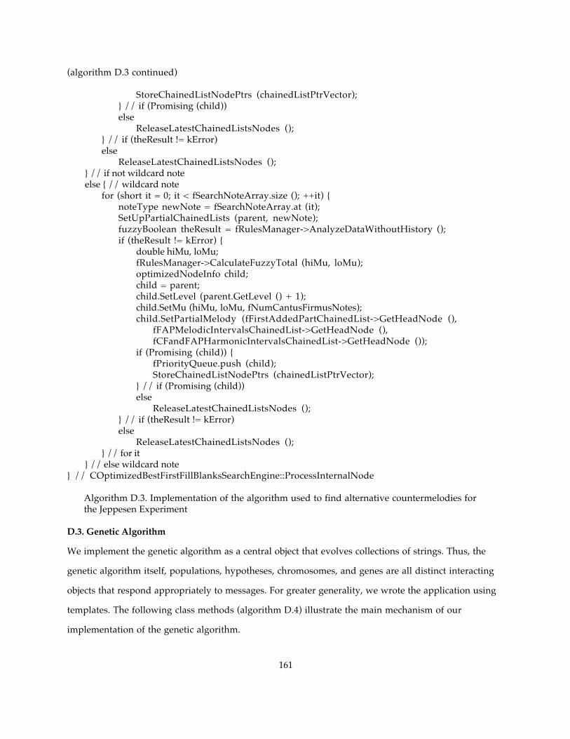
(algorithm D.3 continued)

StoreChainedListNodePtrs (chainedListPtrVector);} // if (Promising (child))else

ReleaseLatestChainedListsNodes ();} // if (theResult != kError)else

ReleaseLatestChainedListsNodes ();} // if not wildcard noteelse { // wildcard note

for (short it = 0; it < fSearchNoteArray.size (); ++it) {noteType newNote = fSearchNoteArray.at (it);SetUpPartialChainedLists (parent, newNote);fuzzyBoolean theResult = fRulesManager->AnalyzeDataWithoutHistory ();if (theResult != kError) {

double hiMu, loMu;fRulesManager->CalculateFuzzyTotal (hiMu, loMu);optimizedNodeInfo child;child = parent;child.SetLevel (parent.GetLevel () + 1);child.SetMu (hiMu, loMu, fNumCantusFirmusNotes); child.SetPartialMelody (fFirstAddedPartChainedList->GetHeadNode (),

fFAPMelodicIntervalsChainedList->GetHeadNode (),fCFandFAPHarmonicIntervalsChainedList->GetHeadNode ());

if (Promising (child)) {fPriorityQueue.push (child);StoreChainedListNodePtrs (chainedListPtrVector);

} // if (Promising (child))else

ReleaseLatestChainedListsNodes ();} // if (theResult != kError)else

ReleaseLatestChainedListsNodes ();} // for it

} // else wildcard note} // COptimizedBestFirstFillBlanksSearchEngine::ProcessInternalNode

Algorithm D.3. Implementation of the algorithm used to find alternative countermelodies for the Jeppesen Experiment

D.3. Genetic Algorithm

We implement the genetic algorithm as a central object that evolves collections of strings. Thus, the

genetic algorithm itself, populations, hypotheses, chromosomes, and genes are all distinct interacting

objects that respond appropriately to messages. For greater generality, we wrote the application using

templates. The following class methods (algorithm D.4) illustrate the main mechanism of our

implementation of the genetic algorithm.

161

template < typename T = default_type, typename T2 = t_ChromosomeType < T >, typename T3 = T > void t_CAbstractGA < T, T2, T3 >::MainEventLoop (void) {

unsigned long numIterations = 0;Evaluate (0);while (fAllTimeBestHypothesis < fFitnessThreshold && numIterations < fMaxIterations) {

fPopulation->CreateNewGeneration ();Evaluate (++numIterations);

} }

template < typename T = default_type, typename T2 = t_ChromosomeType < T >, typename T3 = T > void t_CAbstractGA < T, T2, T3 >::Evaluate (unsigned long iteration) {

vector < t_CHypothesis < T, T2 > >::iterator h;for (h = fPopulation->begin (); h != fPopulation->end (); ++h) {

if (fAllTimeBestHypothesis < * h) { fAllTimeBestHypothesis = * h;

}}

}

template < typename T, typename T2 = t_ChromosomeType < T >, typename T3 = T >void t_AbstractPopulationType < T, T2, T3 >::CreateNewGeneration (void) {

SetUpCycle ();Select ();Crossover ();Mutate ();Update ();

}

template < typename T, typename T2 = t_ChromosomeType < T >, typename T3 = T >void t_AbstractPopulationType < T, T2, T3 >::SetUpCycle (void) {

fWheel->SetUpWheel (*this);fNewGeneration.clear ();fNewGeneration.reserve (fNumHypotheses);

} // t_AbstractPopulationType::SetUpCycle

template < typename T, typename T2 = t_ChromosomeType < T >, typename T3 = T >void t_AbstractPopulationType < T, T2, T3 >::Select (void) {

for (short i = 0; i < fNumElites; ++i) {DoSelect ();

}} // t_AbstractPopulationType::Select

template < typename T, typename T2 = t_ChromosomeType < T >, typename T3 = T >inline void t_AbstractPopulationType < T, T2, T3 >::DoSelect (void) {

fNewGeneration.push_back (at (fWheel->ProbabilisticallySelectedIndex ()));} // t_AbstractPopulationType::DoSelect

162

(algorithm D.4 continued)

template < typename T, typename T2 = t_ChromosomeType < T >, typename T3 = T > void t_AbstractPopulationType < T, T2, T3 >::Crossover (void) {

for (short i = 0; i < fNumCrossoverPairs; ++i) {short index, index2;index = fWheel->ProbabilisticallySelectedIndex (); // choose two chromosomes for crossoverindex2 = fWheel->ProbabilisticallySelectedIndex ();t_CHypothesis < T, T2 > h3 (fChromosomeSize), h4 (fChromosomeSize);DoCrossover (at (index).GetChromosome (), at (index2).GetChromosome (),

h3.GetChromosome (), h4.GetChromosome ());fNewGeneration.push_back (h3);fNewGeneration.push_back (h4);

}} // t_AbstractPopulationType::Crossover

template < typename T, typename T2 = t_ChromosomeType < T >, typename T3 = T >void t_AbstractPopulationType < T, T2, T3 >::Mutate (void) {

for (short i = 0; i < fNumMutations; ++i) {DoMutate (fNewGeneration.at (rand () % fNumHypotheses).GetChromosome ());

} // forif (BiasedToss (fProbabilityOfSingleMutation)) {

DoMutate (fNewGeneration.at (rand () % fNumHypotheses).GetChromosome ());} // if

} // t_AbstractPopulationType::Mutate

template < typename T, typename T2 = t_ChromosomeType < T >, typename T3 = T >void t_AbstractPopulationType < T, T2, T3 >::Update (void) {

std::vector < t_CHypothesis < T, T2 > >::iterator h;for (h = fNewGeneration.begin (); h != fNewGeneration.end (); ++h) {

h->SetFitness (CalculateFitness (Decode (h->GetChromosome ())));}* this = fNewGeneration;stable_sort (begin (), end (), greater < t_CHypothesis < T, T2 > >());

} // t_AbstractPopulationType::Update

template < typename T, typename T2 = t_ChromosomeType < T >, typename T3 = T >inline T2 t_AbstractPopulationType < T, T2, T3 >::Decode (const T2& chromosome) {

return chromosome; } // t_AbstractPopulationType::Decode

template < typename T, typename F, typename T2 = t_ChromosomeType < T >, typename T3 = T >inline double t_BasePopulationType < T, F, T2, T3 >::CalculateFitness (const T2& c) {

return fFitnessFunction (c); } // t_BasePopulationType::CalculateFitness

163

(algorithm D.4 continued)

template < typename T, typename F, typename P = CTautology, typename P2 = P, typename P3 = P, typename T2 = t_ChromosomeType < T >, typename T3 = T >

void CBasePalPop < T, F, P, P2, P3, T2, T3 >::Crossover (void) {// Probabilistic pick couples, for each apply DoCrossover and add offspring to fNewGenerationfor (short i = 0; i < fNumCrossoverPairs; ++i) {

short crossoverIndex;t_CHypothesis < T, T2 > h3 (fChromosomeSize), h4 (fChromosomeSize);unsigned long numFailedAttempts = 0; do {

short index, index2;index = fWheel->ProbabilisticallySelectedIndex ();index2 = fWheel->ProbabilisticallySelectedIndex ();crossoverIndex = DoCrossover (at (index).GetChromosome(), at(index2).GetChromosome (),

h3.GetChromosome (), h4.GetChromosome ());} while ((! fPredicate2 (h3.GetChromosome (), crossoverIndex)

|| ! fPredicate2 (h4.GetChromosome (), crossoverIndex)) && (++numFailedAttempts < fMaxCrossoverTries));

if (numFailedAttempts < fMaxCrossoverTries) {fNewGeneration.push_back (h3);fNewGeneration.push_back (h4);

}else {

short index, index2;index = fWheel->ProbabilisticallySelectedIndex ();index2 = fWheel->ProbabilisticallySelectedIndex ();fNewGeneration.push_back (at (index));fNewGeneration.push_back (at (index2));

}}

} // CBasePalPop::Crossover

template < typename T, typename F, typename P = CTautology, typename P2 = P, typename P3 = P, typename T2 = t_ChromosomeType < T >, typename T3 = T >

inline short CBasePalPop < T, F, P, P2, P3, T2, T3 >::DoCrossover (const T2& c, const T2& c2, T2& c3, T2& c4) {

return c.Crossover (c2, c3, c4); } // CBasePalPop::DoCrossover

template < typename T, typename F, typename P = CTautology, typename P2 = P, typename P3 = P, typename T2 = t_ChromosomeType < T >, typename T3 = T >

inline void CBasePalPop < T, F, P, P2, P3, T2, T3 >::DoMutate (T2& c) { c.MutateWithMaxNumAttempts (fPredicate3);

} // CBasePalPop::DoMutate

Algorithm D.4. Class methods of an object-oriented implementation of the genetic algorithm. DoCrossover, DoMutate, and CalculateFitness are null methods in the abstract class t_AbstractPopulationType, and are defined in descendant classes t_BasePopulationType and CBasePalPop.

164

In an attempt to prevent premature convergence, we employed the technique of fitness scaling

(chapter 6, section 6.2). We designed roulette wheel classes that determined which chromosomes were

to be selected for the next generation. In the subclass “CScaledRouletteWheel,” we overrode the

method “SetUpWheel” (see method “SetUpCycle” in algorithm D.4) to use fitness scaling (algorithm

D.5); this part of the algorithm is based on Goldberg (1989, 79).

template < typename T, typename T2 >void CScaledRouletteWheel < T, T2 >::SetUpWheel (const populationType& population) {

double rawMin, rawMax, rawAvg;FindPopMinMaxAvg (population, rawMin, rawMax, rawAvg);double gradient, intercept; CalculateScalingCoefficients (rawMin, rawMax, rawAvg, gradient, intercept);double frontier = fMin = 0;for (short i = 0; i < population.size (); ++i) {

frontier += (gradient * ( population [ i ].GetFitness () ) + intercept);fWheel [i] = frontier;

} // forfMax = frontier;

} // CScaledRouletteWheel::SetUpWheel

template < typename T, typename T2 >void CScaledRouletteWheel < T, T2 >::FindPopMinMaxAvg (const populationType& population, double& rawMin, double& rawMax, double& rawAvg) {

rawMin = numeric_limits < double >::max (); rawMax = 0;double totalFitness = 0;populationType::const_iterator h;for (h = population.begin (); h != population.end (); ++h) {

double fitness = h->GetFitness ();if (fitness < rawMin) rawMin = fitness;if (fitness > rawMax) rawMax = fitness;totalFitness += fitness;

}rawAvg = (population.size () ? totalFitness / population.size () : 0);

} // CScaledRouletteWheel::FindPopMinMaxAvg

template < typename T, typename T2 >void CScaledRouletteWheel < T, T2 > :: CalculateScalingCoefficients (double rawMin, double rawMax, double rawAvg, double& gradient, double& intercept ) {

double delta;if (rawMin > ( fFitnessMultiple * rawAvg - rawMax) / (fFitnessMultiple - 1.0) ) {

delta = rawMax - rawAvg;gradient = (fFitnessMultiple - 1.0) * rawAvg / delta;intercept = rawAvg * (rawMax - fFitnessMultiple * rawAvg) / delta;

}else {

delta = rawAvg - rawMin;gradient = rawAvg / delta;intercept = -rawMin * rawAvg / delta;

165

(algorithm D.5 continued)

}} // CScaledRouletteWheel::CalculateScalingCoefficients

Algorithm D.5. Fitness scaling in the CScaledRouletteWheel class. The method “SetUpWheel” prepares for its fitness-scaled probabilistic spin by calculating the gradient and intercept through the private method “CalculateScalingCoefficients”.

166

APPENDIX E. OUTPUT OF PROGRAMS USING GENERATE-AND-TEST, BRANCH-AND-BOUND, AND GENETIC ALGORITHMS

We list here the output of the Palestrina application to various cantus firmi, using the exhaustive,

best-first branch-and-bound, and genetic algorithms. These outputs have been referred to in chapters 5

and 6. They are as follows: E.1. Two genetic algorithm outputs to cantus firmus <D, F, E, D, G, F, a, G, F,

E, D>. with rules weighted to favor Jeppesen’s preferences; E.2.1. Genetic algorithm output to cantus

firmus <D, a, G, F, E, D, F, E, D> in second species with one added part; E.2.2. Genetic algorithm output

to cantus firmus <D, a, G, F, E, D, F, E, D> in first species with two added parts; E.3.1. Best-first

algorithm to cantus firmus <d, c, h, c, h, a, h, a, F#, G>, with trained neural network evaluation that is

not non-increasing with respect to partial countermelody length; E.3.2. Best-first algorithm to cantus

firmus <d, c, h, c, h, a, h, a, F#, G>, with trained neural network evaluation that is (almost) non-

increasing with respect to partial countermelody length.

E.1. Two Genetic Algorithm Outputs with Rules Weighted to Favor Jeppesen’s Preferences

Listing E.1 shows the output of the genetic algorithm based on rules weighted according to the instance

of the Jeppesen experiment described in chapter 5, section 5.1, giving preference to the Note Variety

rule. The genetic algorithm produced the optimal countermelody in just seven iterations; this optimal

countermelody is also Jeppesen’s.

Listing E.1. Genetic algorithm output to cantus firmus <D, F, E, D, G, F, a, G, F, E, D> with rules weighted to favor Jeppesen’s choice: optimal countermelodies found in seven iterations

Cantus firmus: D F E D G F a G F E D crossover rate: 0.6 mutation rate: 0.1 max num init tries: 50 max num crossover tries: 20 max num mutation tries: 20 fitness multiple: 1.2 population size: 50 num iterations: 50 elitist model, max num elites: 50Initial hypotheses:chromosome fitnessa a G F E D A B D C# D 0.872727 a aa g f e d e h d c# d 0.872727 a a G F E D A B D C# D 0.872727 a a G F E D C B D C# D 0.854545 aa aa g f e d c h d c# d 0.854545 aa aa g f e d c h d c# d 0.854545 a a G F C D C E D C# D 0.836364 a a c d e f e h d c# d 0.836364 a a G F C D C E D C# D 0.836364 aa d g f e f c e d c# d 0.836364 a a G F C D C E D C# D 0.836364

167

(listing E.1 continued)

aa aa g f e f c e d c# d 0.836364 aa d g f e d e h d c# d 0.836364 a D G F C D C E D C# D 0.836364 a D G F C D C E D C# D 0.836364 D D A F E D C B D C# D 0.818182 d d G a h d c e d c# d 0.818182 d a G a h d c e d c# d 0.818182 d c G a h d c e d c# d 0.818182 a a G a h d c e d c# d 0.818182 D D C F E D A B D C# D 0.818182 a a h d e f c e d c# d 0.818182 d d G a h d c e d c# d 0.818182 a a G a h d c e d c# d 0.818182 d d c d e f e h d c# d 0.8 d d g f e d c e d c# d 0.8 d a e f e d c h d c# d 0.8 d c g f e d c h d c# d 0.8 d d g f e d c e d c# d 0.8 d c e f e d e h d c# d 0.8 d c g f e d c h d c# d 0.8 d d c d e f e h d c# d 0.8 D D G F E D C E D C# D 0.8 a a h d e f e h d c# d 0.781818 d c g f e f c e d c# d 0.781818 a a h d e f e h d c# d 0.781818 d d c d e f c e d c# d 0.763636 d d c f e d c h d c# d 0.763636 d a h d e d c h d c# d 0.763636 d d c f e d c h d c# d 0.763636 D D C F E D C B D C# D 0.763636 d d c f e d c h d c# d 0.763636 d a h d e d c h d c# d 0.763636 d d c f e d c h d c# d 0.763636 d d c f e d c h d c# d 0.763636 d d c d e d c h d c# d 0.745455 d d c f e d c e d c# d 0.745455 D D C F E D C E D C# D 0.745455 d d c f e d c e d c# d 0.745455 C a G F C D C GG D GG a 0

Average fitness: 0.789455

Performing genetic algorithm: Please wait!

iteration fitnessaverage best

local global0. 0.789455 0.872727 0.8727271. 0.750545 0.872727 0.8727272. 0.803636 0.872727 0.8727273. 0.8 0.872727 0.8727274. 0.802182 0.872727 0.8727275. 0.805455 0.872727 0.8727276. 0.796364 0.872727 0.8727277. 0.789091 0.890909 0.8909098. 0.802545 0.890909 0.8909099. 0.808 0.890909 0.89090910. 0.794182 0.890909 0.89090911. 0.803273 0.890909 0.89090912. 0.802182 0.890909 0.890909

168

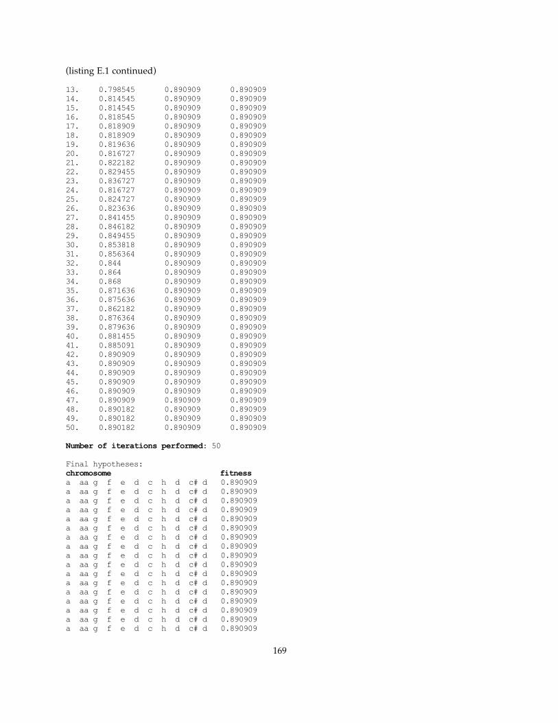
(listing E.1 continued)

13. 0.798545 0.890909 0.89090914. 0.814545 0.890909 0.89090915. 0.814545 0.890909 0.89090916. 0.818545 0.890909 0.89090917. 0.818909 0.890909 0.89090918. 0.818909 0.890909 0.89090919. 0.819636 0.890909 0.89090920. 0.816727 0.890909 0.89090921. 0.822182 0.890909 0.89090922. 0.829455 0.890909 0.89090923. 0.836727 0.890909 0.89090924. 0.816727 0.890909 0.89090925. 0.824727 0.890909 0.89090926. 0.823636 0.890909 0.89090927. 0.841455 0.890909 0.89090928. 0.846182 0.890909 0.89090929. 0.849455 0.890909 0.89090930. 0.853818 0.890909 0.89090931. 0.856364 0.890909 0.89090932. 0.844 0.890909 0.89090933. 0.864 0.890909 0.89090934. 0.868 0.890909 0.89090935. 0.871636 0.890909 0.89090936. 0.875636 0.890909 0.89090937. 0.862182 0.890909 0.89090938. 0.876364 0.890909 0.89090939. 0.879636 0.890909 0.89090940. 0.881455 0.890909 0.89090941. 0.885091 0.890909 0.89090942. 0.890909 0.890909 0.89090943. 0.890909 0.890909 0.89090944. 0.890909 0.890909 0.89090945. 0.890909 0.890909 0.89090946. 0.890909 0.890909 0.89090947. 0.890909 0.890909 0.89090948. 0.890182 0.890909 0.89090949. 0.890182 0.890909 0.89090950. 0.890182 0.890909 0.890909

Number of iterations performed: 50

Final hypotheses:chromosome fitnessa aa g f e d c h d c# d 0.890909 a aa g f e d c h d c# d 0.890909 a aa g f e d c h d c# d 0.890909 a aa g f e d c h d c# d 0.890909 a aa g f e d c h d c# d 0.890909 a aa g f e d c h d c# d 0.890909 a aa g f e d c h d c# d 0.890909 a aa g f e d c h d c# d 0.890909 a aa g f e d c h d c# d 0.890909 a aa g f e d c h d c# d 0.890909 a aa g f e d c h d c# d 0.890909 a aa g f e d c h d c# d 0.890909 a aa g f e d c h d c# d 0.890909 a aa g f e d c h d c# d 0.890909 a aa g f e d c h d c# d 0.890909 a aa g f e d c h d c# d 0.890909 a aa g f e d c h d c# d 0.890909

169

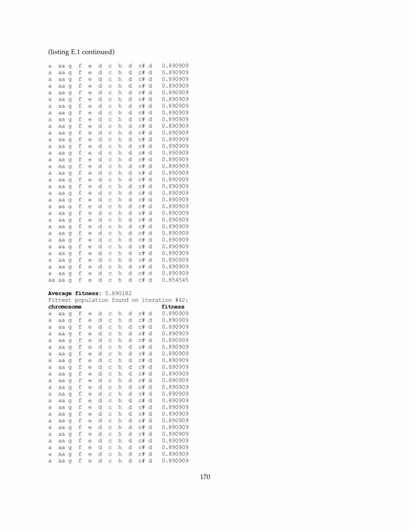
(listing E.1 continued)

a aa g f e d c h d c# d 0.890909 a aa g f e d c h d c# d 0.890909 a aa g f e d c h d c# d 0.890909 a aa g f e d c h d c# d 0.890909 a aa g f e d c h d c# d 0.890909 a aa g f e d c h d c# d 0.890909 a aa g f e d c h d c# d 0.890909 a aa g f e d c h d c# d 0.890909 a aa g f e d c h d c# d 0.890909 a aa g f e d c h d c# d 0.890909 a aa g f e d c h d c# d 0.890909 a aa g f e d c h d c# d 0.890909 a aa g f e d c h d c# d 0.890909 a aa g f e d c h d c# d 0.890909 a aa g f e d c h d c# d 0.890909 a aa g f e d c h d c# d 0.890909 a aa g f e d c h d c# d 0.890909 a aa g f e d c h d c# d 0.890909 a aa g f e d c h d c# d 0.890909 a aa g f e d c h d c# d 0.890909 a aa g f e d c h d c# d 0.890909 a aa g f e d c h d c# d 0.890909 a aa g f e d c h d c# d 0.890909 a aa g f e d c h d c# d 0.890909 a aa g f e d c h d c# d 0.890909 a aa g f e d c h d c# d 0.890909 a aa g f e d c h d c# d 0.890909 a aa g f e d c h d c# d 0.890909 a aa g f e d c h d c# d 0.890909 a aa g f e d c h d c# d 0.890909 a aa g f e d c h d c# d 0.890909 a aa g f e d c h d c# d 0.890909 aa aa g f e d c h d c# d 0.854545

Average fitness: 0.890182Fittest population found on iteration #42:chromosome fitnessa aa g f e d c h d c# d 0.890909 a aa g f e d c h d c# d 0.890909 a aa g f e d c h d c# d 0.890909 a aa g f e d c h d c# d 0.890909 a aa g f e d c h d c# d 0.890909 a aa g f e d c h d c# d 0.890909 a aa g f e d c h d c# d 0.890909 a aa g f e d c h d c# d 0.890909 a aa g f e d c h d c# d 0.890909 a aa g f e d c h d c# d 0.890909 a aa g f e d c h d c# d 0.890909 a aa g f e d c h d c# d 0.890909 a aa g f e d c h d c# d 0.890909 a aa g f e d c h d c# d 0.890909 a aa g f e d c h d c# d 0.890909 a aa g f e d c h d c# d 0.890909 a aa g f e d c h d c# d 0.890909 a aa g f e d c h d c# d 0.890909 a aa g f e d c h d c# d 0.890909 a aa g f e d c h d c# d 0.890909 a aa g f e d c h d c# d 0.890909 a aa g f e d c h d c# d 0.890909 a aa g f e d c h d c# d 0.890909

170

(listing E.1 continued)

a aa g f e d c h d c# d 0.890909 a aa g f e d c h d c# d 0.890909 a aa g f e d c h d c# d 0.890909 a aa g f e d c h d c# d 0.890909 a aa g f e d c h d c# d 0.890909 a aa g f e d c h d c# d 0.890909 a aa g f e d c h d c# d 0.890909 a aa g f e d c h d c# d 0.890909 a aa g f e d c h d c# d 0.890909 a aa g f e d c h d c# d 0.890909 a aa g f e d c h d c# d 0.890909 a aa g f e d c h d c# d 0.890909 a aa g f e d c h d c# d 0.890909 a aa g f e d c h d c# d 0.890909 a aa g f e d c h d c# d 0.890909 a aa g f e d c h d c# d 0.890909 a aa g f e d c h d c# d 0.890909 a aa g f e d c h d c# d 0.890909 a aa g f e d c h d c# d 0.890909 a aa g f e d c h d c# d 0.890909 a aa g f e d c h d c# d 0.890909 a aa g f e d c h d c# d 0.890909 a aa g f e d c h d c# d 0.890909 a aa g f e d c h d c# d 0.890909 a aa g f e d c h d c# d 0.890909 a aa g f e d c h d c# d 0.890909 a aa g f e d c h d c# d 0.890909 Its average fitness: 0.890909List of successively fitter hypotheses as the population evolved:a a G F E D A B D C# D 0.872727 0a aa g f e d c h d c# d 0.890909 7Best hypothesis first found:

a aa g f e d c h d c# d 0.890909 7

Another run of the genetic algorithm, this time using a smaller population size (20), also produced the

optimal countermelody. Here we also asked the program to append information on the chromosomes to

enable us to track the evolution of the individual chromosomes (INITIAL: chromosome created in the

initial population; SELECTION: chromosome probabilistically selected from the previous generation

[followed by the number of the chromosome in that previous generation]; CROSSOVER: chromosome

created by crossover [ordinal number of the parents also indicated]; MUTATION: chromosome created

by mutation). See chapter 6, section 6.2 for an outline of the evolution of the optimal countermelody

(Jeppesen’s choice: <a, aa, g, f, e, d, c, h, d, c#, d>).

Listing E.2. Genetic algorithm output to cantus firmus <D, F, E, D, G, F, a, G, F, E, D> with rules weighted to favor Jeppesen’s choice: optimal countermelodies found in three iterations. Shown also is additional information to enable tracking of ancestry of individual chromosomes.

Cantus firmus: D F E D G F a G F E D crossover rate: 0.6 mutation rate: 0.1 max num init tries: 50

171

(listing E.2 continued)

max num crossover tries: 20 max num mutation tries: 20 fitness multiple: 1.2 population size: 20 num iterations: 50 elitist model, max num elites: 20Initial hypotheses:chromosome fitness operationa aa g f e f e h d c# d 0.872727 INITIAL a D G F C D C E D C# D 0.836364 INITIAL aa f g f e f e h d c# d 0.836364 INITIAL d a c d e f e h d c# d 0.836364 INITIAL aa d g f e f e h d c# d 0.836364 INITIAL a a G F C D C E D C# D 0.836364 INITIAL d c G a h d c e d c# d 0.818182 INITIAL d a G a h d c e d c# d 0.818182 INITIAL d a G a h d c e d c# d 0.818182 INITIAL d a G a h d c e d c# d 0.818182 INITIAL D D A F E D A B D C# D 0.8 INITIAL d a e f e d c h d c# d 0.8 INITIAL a a e f e d c h d c# d 0.8 INITIAL a a h d e f e h d c# d 0.781818 INITIAL d c e f e d c h d c# d 0.781818 INITIAL d a c d e d c h d c# d 0.781818 INITIAL d d c f e d c h d c# d 0.763636 INITIAL d a h d e d c h d c# d 0.763636 INITIAL a a h d e d c h d c# d 0.763636 INITIAL d d c d e d c h d c# d 0.745455 INITIAL

Average fitness: 0.805455

Performing genetic algorithm: Please wait!

iteration fitnessaverage best

local global0. 0.81 0.87 0.871. 0.80 0.87 0.872. 0.81 0.87 0.873. 0.74 0.89 0.894. 0.84 0.89 0.895. 0.72 0.89 0.896. 0.82 0.89 0.897. 0.86 0.89 0.898. 0.87 0.89 0.899. 0.83 0.89 0.8910. 0.86 0.89 0.8911. 0.85 0.89 0.8912. 0.86 0.89 0.8913. 0.86 0.89 0.8914. 0.89 0.89 0.8915. 0.89 0.89 0.8916. 0.89 0.89 0.8917. 0.89 0.89 0.8918. 0.89 0.89 0.8919. 0.89 0.89 0.8920. 0.89 0.89 0.8921. 0.89 0.89 0.8922. 0.89 0.89 0.8923. 0.89 0.89 0.89

172

(listing E.2 continued)

24. 0.89 0.89 0.8925. 0.89 0.89 0.8926. 0.89 0.89 0.8927. 0.89 0.89 0.8928. 0.89 0.89 0.8929. 0.85 0.89 0.8930. 0.89 0.89 0.8931. 0.89 0.89 0.8932. 0.89 0.89 0.8933. 0.85 0.89 0.8934. 0.89 0.89 0.8935. 0.85 0.89 0.8936. 0.89 0.89 0.8937. 0.89 0.89 0.8938. 0.85 0.89 0.8939. 0.89 0.89 0.8940. 0.89 0.89 0.8941. 0.89 0.89 0.8942. 0.89 0.89 0.8943. 0.89 0.89 0.8944. 0.85 0.89 0.8945. 0.89 0.89 0.8946. 0.89 0.89 0.8947. 0.89 0.89 0.8948. 0.89 0.89 0.8949. 0.89 0.89 0.8950. 0.89 0.89 0.89

Number of iterations performed: 50

Final hypotheses:chromosome fitness operation ancestrya aa g f e d c h d c# d 0.89 SELECTION 8 a aa g f e d c h d c# d 0.89 SELECTION 12 a aa g f e d c h d c# d 0.89 SELECTION 18 a aa g f e d c h d c# d 0.89 SELECTION 4 a aa g f e d c h d c# d 0.89 SELECTION 15 a aa g f e d c h d c# d 0.89 SELECTION 5 a aa g f e d c h d c# d 0.89 SELECTION 8 a aa g f e d c h d c# d 0.89 SELECTION 18 a aa g f e d c h d c# d 0.89 CROSSOVER 14 3 a aa g f e d c h d c# d 0.89 CROSSOVER 14 3 MUTATION a aa g f e d c h d c# d 0.89 CROSSOVER 13 19 a aa g f e d c h d c# d 0.89 CROSSOVER 13 19 a aa g f e d c h d c# d 0.89 CROSSOVER 5 17 a aa g f e d c h d c# d 0.89 CROSSOVER 5 17 MUTATION a aa g f e d c h d c# d 0.89 CROSSOVER 2 14 a aa g f e d c h d c# d 0.89 CROSSOVER 2 14 a aa g f e d c h d c# d 0.89 CROSSOVER 7 4 a aa g f e d c h d c# d 0.89 CROSSOVER 7 4 a aa g f e d c h d c# d 0.89 CROSSOVER 8 16 a aa g f e d c h d c# d 0.89 CROSSOVER 8 16

Average fitness: 0.89Fittest population found on iteration #15:chromosome fitness operation ancestrya aa g f e d c h d c# d 0.89 SELECTION 8 a aa g f e d c h d c# d 0.89 SELECTION 12 a aa g f e d c h d c# d 0.89 SELECTION 10 a aa g f e d c h d c# d 0.89 SELECTION 5

173

(listing E.2 continued)

a aa g f e d c h d c# d 0.89 SELECTION 0 a aa g f e d c h d c# d 0.89 SELECTION 14 a aa g f e d c h d c# d 0.89 SELECTION 17 a aa g f e d c h d c# d 0.89 SELECTION 14 a aa g f e d c h d c# d 0.89 CROSSOVER 8 0 a aa g f e d c h d c# d 0.89 CROSSOVER 8 0 a aa g f e d c h d c# d 0.89 CROSSOVER 16 9 a aa g f e d c h d c# d 0.89 CROSSOVER 16 9 a aa g f e d c h d c# d 0.89 CROSSOVER 2 0 a aa g f e d c h d c# d 0.89 CROSSOVER 2 0 a aa g f e d c h d c# d 0.89 CROSSOVER 11 10 a aa g f e d c h d c# d 0.89 CROSSOVER 11 10 a aa g f e d c h d c# d 0.89 CROSSOVER 9 7 MUTATION a aa g f e d c h d c# d 0.89 CROSSOVER 9 7 a aa g f e d c h d c# d 0.89 CROSSOVER 10 7 a aa g f e d c h d c# d 0.89 CROSSOVER 10 7 Its average fitness: 0.89List of successively fitter hypotheses as the population evolved:a aa g f e f e h d c# d 0.87 INITIAL 0a aa g f e d c h d c# d 0.89 CROSSOVER 17 1 3Best hypothesis first found:a aa g f e d c h d c# d 0.89 CROSSOVER 17 1 3

****0. 0.81, 0.87, 0.87chromosome fitness operation

0. a aa g f e f e h d c# d 0.87 INITIAL 1. a D G F C D C E D C# D 0.84 INITIAL 2. aa f g f e f e h d c# d 0.84 INITIAL 3. d a c d e f e h d c# d 0.84 INITIAL 4. aa d g f e f e h d c# d 0.84 INITIAL 5. a a G F C D C E D C# D 0.84 INITIAL 6. d c G a h d c e d c# d 0.82 INITIAL 7. d a G a h d c e d c# d 0.82 INITIAL 8. d a G a h d c e d c# d 0.82 INITIAL 9. d a G a h d c e d c# d 0.82 INITIAL 10. D D A F E D A B D C# D 0.80 INITIAL 11. d a e f e d c h d c# d 0.80 INITIAL 12. a a e f e d c h d c# d 0.80 INITIAL 13. a a h d e f e h d c# d 0.78 INITIAL 14. d c e f e d c h d c# d 0.78 INITIAL 15. d a c d e d c h d c# d 0.78 INITIAL 16. d d c f e d c h d c# d 0.76 INITIAL 17. d a h d e d c h d c# d 0.76 INITIAL 18. a a h d e d c h d c# d 0.76 INITIAL 19. d d c d e d c h d c# d 0.75 INITIAL ***1. 0.80, 0.87, 0.87

chromosome fitness operation ancestry 0. a aa g f e f e h d c# d 0.87 CROSSOVER 0 4 1. a a G F E D C E D C# D 0.84 SELECTION 5 MUTATION 2. aa d g f e f e h d c# d 0.84 SELECTION 4 3. aa f g f e f e h d c# d 0.84 CROSSOVER 4 2 4. aa d g f e f e h d c# d 0.84 CROSSOVER 4 2 5. aa d g f e f e h d c# d 0.84 CROSSOVER 0 4 6. d a c d e f e h d c# d 0.84 CROSSOVER 3 12 7. d a G a h d c e d c# d 0.82 CROSSOVER 8 16 8. D D A F E D A B D C# D 0.80 SELECTION 10 9. D D A F E D A B D C# D 0.80 SELECTION 10 10. a a e f e d c h d c# d 0.80 SELECTION 12 11. d a e f e d c h d c# d 0.80 CROSSOVER 19 11 12. a a e f e d c h d c# d 0.80 CROSSOVER 3 12

174

(listing E.2 continued)

13. a a h d e f e h d c# d 0.78 SELECTION 13 14. d c e f e d c h d c# d 0.78 CROSSOVER 14 18 15. d a h d e d c h d c# d 0.76 SELECTION 15 MUTATION 16. a a h d e d c h d c# d 0.76 CROSSOVER 14 18 17. d d c f e d c h d c# d 0.76 CROSSOVER 8 16 18. d d c d e d c h d c# d 0.75 SELECTION 19 19. d d c d e d c h d c# d 0.75 CROSSOVER 19 11 ****2. 0.81, 0.87, 0.87

chromosome fitness operation ancestry 0. a aa g f e f e h d c# d 0.87 SELECTION 0 MUTATION 1. a aa g f e f e h d c# d 0.87 CROSSOVER 2 0 2. aa d g f e f e h d c# d 0.84 SELECTION 2 3. aa d g f e f e h d c# d 0.84 SELECTION 5 4. aa d g f e f e h d c# d 0.84 CROSSOVER 2 0 5. aa d g f e f e h d c# d 0.84 CROSSOVER 5 10 6. a a c d e f e h d c# d 0.84 CROSSOVER 10 6 MUTATION 7. aa d g f e f e h d c# d 0.84 CROSSOVER 5 4 8. aa d g f e f e h d c# d 0.84 CROSSOVER 5 4 9. d a e f e d c h d c# d 0.80 SELECTION 11 10. D D A F E D A B D C# D 0.80 SELECTION 9 11. d a e f e d c h d c# d 0.80 CROSSOVER 14 11 12. a a e f e d c h d c# d 0.80 CROSSOVER 5 10 13. d a e f e d c h d c# d 0.80 CROSSOVER 10 6 14. a a e f e d c h d c# d 0.80 CROSSOVER 16 12 15. a a h d e f e h d c# d 0.78 SELECTION 13 16. a a h d e f e h d c# d 0.78 SELECTION 13 17. d c e f e d c h d c# d 0.78 CROSSOVER 14 11 18. d a h d e d c h d c# d 0.76 SELECTION 15 19. a a h d e d c h d c# d 0.76 CROSSOVER 16 12 ***3. 0.74, 0.89, 0.89

chromosome fitness operation ancestry 0. a aa g f e d c h d c# d 0.89 CROSSOVER 17 1 1. a aa g f e f e h d c# d 0.87 SELECTION 0 MUTATION 2. a aa g f e f e h d c# d 0.87 CROSSOVER 1 14 3. a aa g f e f e h d c# d 0.87 CROSSOVER 7 0 4. aa d g f e d c h d c# d 0.85 CROSSOVER 12 3 5. aa d g f e f e h d c# d 0.84 SELECTION 5 6. aa d g f e f e h d c# d 0.84 CROSSOVER 7 0 7. aa d g f e f e h d c# d 0.84 CROSSOVER 12 2 8. a a e f e d c h d c# d 0.80 SELECTION 12 9. a a e f e d c h d c# d 0.80 SELECTION 14 10. a a e f e d c h d c# d 0.80 SELECTION 12 MUTATION 11. a a e f e d c h d c# d 0.80 CROSSOVER 1 14 12. a a e f e d c h d c# d 0.80 CROSSOVER 12 2 13. a a e f e d c h d c# d 0.80 CROSSOVER 12 16 14. d c e f e d c h d c# d 0.78 SELECTION 17 15. a a h d e f e h d c# d 0.78 SELECTION 15 16. a a h d e f e h d c# d 0.78 SELECTION 15 17. a a h d e f e h d c# d 0.78 CROSSOVER 12 16 18. d c e f e f e h d c# d 0.00 CROSSOVER 17 1

19. a a e f e f e h d c# d 0.00 CROSSOVER 12 3

175

E.1.1. Average Schema and Population Fitness, and Estimated Bounds on Occurrences of Instances

The following tables (E.1–3) shows the average schema and population fitness, derived from the second

run of the genetic algorithm to cantus firmus <D, F, E, D, G, F, a, G, F, E, D> as described in section E.1.

We used this to estimate the lower- and upper-bounds on occurrences of representatives of schemata “a

aa * * * * * * * * *”, “* * g f e * * * * * *”, and “* * * * * * * h d c# d” (chapter 6, section 6.2.1).

Table E.1. Average schema and population fitness, and estimated bounds of schema (a) “a aa * * * * * * * * *”; (b) “* * g f e * * * * * *”; (c) “* * * * * * * h d c# d”

(a) Schema “a aa * * * * * * * * *”

t schema pop- schema lower upper schemafitness ulation occurrence bound bound occurrence(s, t-1) fitness (s, t-1) estimate estimate (s, t)

(t-1) [schema [schemaoccurrence occurrence(s, t)] (s, t)]

1 0.87 0.81 1 0.82 1.07 12 0.87 0.80 1 0.83 1.09 23 0.87 0.81 2 1.64 2.15 44 0.88 0.74 4 3.60 4.73 75 0.87 0.84 7 5.54 7.27 86 0.88 0.72 8 7.42 9.75 107 0.88 0.82 10 8.21 10.78 118 0.89 0.86 11 8.61 11.31 109 0.89 0.87 10 7.79 10.23 1210 0.82 0.83 12 8.98 11.80 711 0.89 0.86 7 5.52 7.24 412 0.89 0.85 4 3.19 4.19 713 0.89 0.86 7 5.52 7.24 1014 0.89 0.86 10 7.88 10.35 1815 0.89 0.89 18 13.71 18.00 2016 0.89 0.89 20 15.23 20.00 2017 0.89 0.89 20 15.23 20.00 2018 0.89 0.89 20 15.23 20.00 2019 0.89 0.89 20 15.23 20.00 2020 0.89 0.89 20 15.23 20.00 20

176

(table E.1 continued)

(b) Schema “* * g f e * * * * * *”

t schema pop- schema lower upper schemafitness ulation occurrence bound bound occurrence(s, t-1) fitness (s, t-1) estimate estimate (s, t)

(t-1) [schema [schemaoccurrence occurrence(s, t)] (s, t)]

1 0.85 0.81 3 2.02 3.15 52 0.85 0.80 5 3.39 5.29 83 0.85 0.81 8 5.37 8.37 84 0.86 0.74 8 5.96 9.28 125 0.86 0.84 12 7.89 12.30 136 0.87 0.72 13 10.04 15.65 167 0.87 0.82 16 10.91 17.00 178 0.87 0.86 17 11.06 17.23 189 0.87 0.87 18 11.57 18.03 1810 0.78 0.83 18 10.85 16.92 1611 0.87 0.86 16 10.35 16.14 1412 0.86 0.85 14 9.10 14.19 1613 0.87 0.86 16 10.35 16.14 1614 0.88 0.86 16 10.44 16.28 2015 0.89 0.89 20 12.83 20.00 2016 0.89 0.89 20 12.83 20.00 2017 0.89 0.89 20 12.83 20.00 2018 0.89 0.89 20 12.83 20.00 2019 0.89 0.89 20 12.83 20.00 2020 0.89 0.89 20 12.83 20.00 20

177

(table E.1 continued)

(c) Schema “* * * * * * * h d c# d”

t schema pop- schema lower upper schemafitness ulation occurrence bound bound occurrence(s, t-1) fitness (s, t-1) estimate estimate (s, t)

(t-1) [schema [schemaoccurrence occurrence(s, t)] (s, t)]

1 0.80 0.81 13 6.88 12.80 162 0.80 0.80 16 8.61 16.01 193 0.81 0.81 19 10.28 19.11 204 0.74 0.74 20 10.76 20.0 205 0.84 0.84 20 10.76 20.0 206 0.72 0.72 20 10.76 20.0 207 0.82 0.82 20 10.76 20.0 208 0.86 0.86 20 10.76 20.0 209 0.87 0.87 20 10.76 20.0 2010 0.87 0.83 19 10.69 19.87 2011 0.86 0.86 20 10.76 20.0 2012 0.85 0.85 20 10.76 20.0 2013 0.86 0.86 20 10.76 20.0 2014 0.86 0.86 20 10.76 20.0 2015 0.89 0.89 20 10.76 20.0 2016 0.89 0.89 20 10.76 20.0 2017 0.89 0.89 20 10.76 20.0 2018 0.89 0.89 20 10.76 20.0 2019 0.89 0.89 20 10.76 20.0 2020 0.89 0.89 20 10.76 20.0 20

E.2. Genetic Algorithm Performance in Second Species, and First Species in Three Parts

We assess the performance of the genetic algorithm in the following two sections in more complex forms

of species counterpoint, namely, second species in two parts, and first species in three parts. The number

of possible solutions is considerably increased; for example, there are thousands of optimal solutions to

the first instance below.

E.2.1. Output to Cantus Firmus <D, a, G, F, E, D, F, E, D> in Second Species with One Added Part

Despite an initial population with very low average fitness, the genetic algorithm succeeded in finding

several near-optimal countermelodies within 50 iterations (compared to Jeppesen’s solution, which the

fuzzified rules gave a score of 0.99: see example 6.9). Notice that the single valid countermelody in the

178

initial population is not optimal, so the optimal countermelodies all must have evolved from either

crossover or mutation.

Listing E.3. Genetic algorithm output to cantus firmus <D, a, G, F, E, D, F, E, D> in second species, one added part

Cantus firmus: D a G F E D F E DAlpha cut: 0Lewin's rule (second species) ro1: 1 w: 1 bonus: 0Law of recovery ro1: 1 w: 1 bonus: 0Outline tritone in four ro1: 1 w: 1 bonus: 0Harmonic range ro1: 1 w: 1 bonus: 0Unisons (second species) ro1: 1 w: 1 bonus: 0Simul skip same direction ro1: 1 w: 1 bonus: 0Unisons on weak beats approached by leap (second species) ro1: 1 w: 1 bonus: 0 crossover rate: 0.6 mutation rate: 0.1 max num init tries: 50 max num crossover tries: 20 max num mutation tries: 20 fitness multiple: 1.2 population size: 100 num iterations: 50 max num no change before stopping: 3 elitist modelInitial hypotheses:chromosome fitness a f c d e E a b c G F a c F E C# D 0.97 h g c g e E c h e E F D d f e c# d 0 c# h E aa A R h a h a G F C Bb F D a 0 GG c# GG R h R aa g Bb Bb e a G F d c# d 0 FF d D d d c a h G F FF c F aa A C# D 0 A f# a D C# g E D Bb D B e d GG d e a 0 B g C FF B f E F G F D d f d e aa a 0 GG C c a Bb c F f# a A D FF E e c# c# d 0 c F h f B F b G c B A e a d e c# d 0 E A Bb B h c d h c F b G B D C# C# D 0 c# FF R FF FF E R G FF a aa C g f e c# d 0 A c h F FF f# G a G F e f E a a c a 0 e G d R G a C# aa h h A Bb G a e R a 0 D G F D F G E c h c# g aa C f# b f a 0 f# A GG d g f# e g c b a h a e a G D 0 e R Bb A B h a R FF C F E a h c# c# d 0 a d B A C B c# G h c h B D C A FF a 0 C# E D F D b F G d c# E a c# C a h a 0 d Bb h c h E d C F g F Bb B E e a a 0 R c# B A GG A C FF A C GG D A D E C# D 0 B b FF F E a D aa Bb F f d f aa g aa a 0 FF C g Bb e FF Bb FF A GG FF A FF C R Bb a 0 GG B R GG G C D E F G d G C Bb d c# d 0 f# C C Bb C# Bb b a D E G C e c C c a 0 E F F C# FF Bb c# h FF h h b c g B C# D 0 R G e d E C# e C F C B h C# c# C c a 0 g R C Bb R FF c R c# FF g c h d e c# d 0 F f h F f# h aa aa B R G f D E FF f# a 0 FF R aa f# C# F c# GG C# a FF G c# G GG aa a 0 R a R B R FF Bb B G F E C A D C# C# D 0 R f h f# g D Bb E c C F FF F D C d d 0 c# F C c h a F c B h B A G F C C a 0 E F aa FF Bb G d aa B A E h E c g R a 0

179

(listing E.3 continued)

B G b a d F a c B GG FF FF A B d c# d 0 e c aa e a G R Bb D g R c# f# e A C# D 0 a d G D b F c h a FF F b B A C# D a 0 f D b a b F FF GG C Bb A D GG G d c# d 0 a F GG g GG d C A GG E f A a c# D C# D 0 Bb e c d D F c f c b a f b C E C# D 0 d G b a h B E D C# d D E F E C# C# D 0 c e h g d a h Bb d c# G F C c d e a 0 f# g e GG G GG A FF C GG Bb GG A B C# C# D 0 D a E G C F a E c b a F Bb b B C# D 0 Bb A g g FF A c# C A F a G F FF a c# d 0 Bb c A G Bb GG B C f a d c h c# d D a 0 c c G h b f c# GG d a F D h E e c# d 0 c d e d R G A g b f c F e f# a c# d 0 R e C# f f# d aa C A C FF F h a E h d 0 R D A C GG A Bb FF F E E D GG A D C# D 0 b A F f c# F D C# B C B h B A E C# D 0 C# C c b A B G d Bb D a A Bb B E C# D 0 f# g F R Bb aa B B f# D R C# E E C# C# D 0 D E F D C E E g G c d aa f c e c# d 0 c c C c g f b G aa g c C C G h c# d 0 E a A A A E D F C d G a B B GG D a 0 a h c E C c a f e c# e h c G c R a 0 C# GG f# D b E a D e B E g f B E C# D 0 R G R f# FF c c d a f G G C# e B F a 0 Bb GG g d b FF aa C# h Bb C c# B c# aa f# a 0 b F g D G f B GG B A C A h c h c# d 0 B C b aa R F A g f# B f c# F f Bb B a 0 A B b Bb Bb Bb c B f g f C# E g D C# D 0 D B A E a h c C A C D a GG R D C# D 0 c# aa h g D h e e d D GG FF C B A C# D 0 c# e C# C# C f# FF c# f# c# a C B b C# f a 0 F FF f# b D c# f# b B c GG a B C# Bb f# a 0 C C c a b Bb D F D C# A a A B C# C# D 0 a d h G R g GG C h GG e e h c# d c# d 0 g g c f# B FF g e f# c D FF A E aa FF a 0 a g c D e a F FF GG D b F Bb G E Bb a 0 GG g aa R aa g g R R a g A C# FF aa f# a 0 d aa e aa e Bb e FF f# F D d g c b f a 0 f d E b D C# c# B B f E a F h A C# D 0 b C c# R FF F b e f f G F B E h e a 0 E a c# g f aa f c E B g FF E e c F a 0 a g E c h e d D E D d e c a h c# d 0 C D C d G d a h c b a h a F E C# D 0 a C# E c A Bb B A D G h B D Bb A C# D 0 Bb aa a c# c C G E b a f aa h c d c# d 0 GG G Bb Bb c# g A C C E d f# B D A C# D 0 d D A Bb C G F FF C A F E D G E C# D 0 FF F FF c Bb Bb G g d h d h c h a c# d 0 h g aa a c# GG e A FF b D h F f g Bb a 0 F b c# B g b R C# c g b e h aa A C# D 0 D a h e d g aa f a c# E h d D E C# D 0 C FF R A C FF FF R a FF e a d c e c# d 0 E B d a h d a G R f# C C E c e c# d 0 h B e g F a C c h c d D d B F a a 0 c# c# GG F C# G g E c a C B D C B C# D 0 aa R g c# Bb h C# A aa d h E h a e c# a 0 F e a e h c d b F R g e aa e F f# a 0 c# E D a d FF C R F a F D E a A R a 0 f e b h d C# E h c D G F h d c# c# d 0

180

(listing E.3 continued)

FF G C R F G F D G D e h g d c# c# d 0 h F e f# R FF f FF b d E e D f# f# B a 0 aa f c E FF Bb aa C Bb e R A e e E e a 0 D F GG R A Bb GG FF A Bb C Bb E h G FF a 0 b GG F a GG B e B a E h B A B C# C# D 0 aa FF h c# g D b e FF c# f D b f B C# D 0 a B d f C# C# e F c# f a A Bb e c# c# d 0

Average fitness: 0.0097

Optimal countermelodies Grade Iteration 1. a f c d e E a b c G F a D F E C# D 0.99 162. d f c d e E a b c G F a D F E C# D 0.99 223. a f c d e h a b c G F a D F E C# D 0.99 224. a f c d e E a h c G F a D F E C# D 0.99 265. a f c d e d a b c G F a D F E C# D 0.99 276. d f c d e h a b c G F a D F E C# D 0.99 297. a d c d e E a b c G F a D F E C# D 0.99 308. a f c d e h a h c G F a D F E C# D 0.99 329. a b c f e E a b c G F a D F E C# D 0.99 3410. d f c d e E a h c G F a D F E C# D 0.99 4011. a d c d e h a h c G F a D F E C# D 0.99 4112. d f c d e d a b c G F a D F E C# D 0.99 4113. d f c d e h a h c G F a D F E C# D 0.99 4414. a f c d e h a d c G F a D F E C# D 0.99 4615. d b c f e E a b c G F a D F E C# D 0.99 4616. d f c d e d a h c G F a D F E C# D 0.99 4617. a h c d e E a b c G F a D F E C# D 0.99 4818. a b c f e E a h c G F a D F E C# D 0.99 4919. a b c d e E a b c G F a D F E C# D 0.99 49

20. a d c d e h a b c G F a D F E C# D 0.99 50

E.2.2. Output to Cantus Firmus <D, a, G, F, E, D, F, E, D> in First Species with Two Added Parts

As with E.2.1, the initial population has very low average fitness, also containing only one valid

countermelody. Again, the near-optimal countermelodies produced in this run of the genetic algorithm

must have evolved from either crossover or mutation.

Listing E.4. Genetic algorithm output to cantus firmus <D, a, G, F, E, D, F, E, D> in first species, two added parts

Cantus firmus: D a G F E D F E DAlpha cut: 0Lewin's rule ro1: 1 w: 1 bonus: 0Stepwise motion should predominate ro1: 1 w: 1 bonus: 0Law of recovery ro1: 1 w: 1 bonus: 0Unisons ro1: 1 w: 1 bonus: 0Simul skip same direction ro1: 1 w: 1 bonus: 0 crossover rate: 0.6 mutation rate: 0.1 max num init tries: 50 max num crossover tries: 20 max num mutation tries: 20 fitness multiple: 1.2 population size: 100 num iterations: 50

181

(listing E.4 continued)

max num no change before stopping: 3 elitist modelInitial hypotheses:chromosome fitness d D G a G F D C# D a d e f c d aa a d 0.89 b f# e F f C G e f B C C C# c GG GG c# c# 0 g C A g FF D D h b f d C FF d c g c# h 0 FF D b C# GG g R aa R c# A G d e h C# f GG 0 c# aa g Bb a f aa R C FF f C Bb A a F D FF 0 G aa C c a G b A a G h E A C B C c# d 0 E f# g d E F c e d c# D G C G c A a E 0 a FF b e d g G D GG D R f# E B B a R c 0 GG f e h c C# C# B g f f R Bb aa GG C# f d 0 f E h R c# GG D C# C# C# e e a C h a c# c# 0 c aa f A e G a f d e E Bb F f Bb D Bb D 0 f# R E R Bb g aa g d G c# R E f Bb a d a 0 c h a b C# GG c b F E aa B R f E aa R d 0 D R F C C# D b e c aa c# e B aa FF B C R 0 A e d a C b f A a c# Bb FF d R E h C# D 0 G e h f# f# F c c# D h c b d B a F B a 0 h aa h D e GG GG d C# R F A D B C F e f 0 B A B FF d F c G Bb FF C g aa aa d aa R h 0 D F b c C R a G d A c G A a G A B D 0 GG F h c# e f F R b a h g aa G a f C# h 0 e f h aa h c# aa g h E h C E e aa f# E C 0 D g b E R E F Bb D a C c E FF f a D GG 0 R d b a c F b C a D F G d e f b c D 0 D c C Bb B C# c F F f# A F f# FF A a d G 0 c# aa A f# d f B Bb aa F c# a E GG B b F a 0 C# A E B C# R GG A D B E C E A C# A c# d 0 D c# GG G G c E FF a aa E d R GG G c D d 0 Bb F D D F d c# C# a GG d f# G Bb E e A D 0

182

(listing E.4 continued)

R f FF aa D e Bb c# d FF B FF FF g aa f C# a 0 R c# GG h c# b c a a A FF R B f# F f c d 0 A aa D D d aa F C Bb aa C# F FF b c# a c# A 0 h F G D d F c e C GG d e c h b a F g 0 a d R GG C FF A F d f C# GG aa G GG C GG D 0 C A C# FF R GG D C# d h A E a F B D R a 0 E h c# R aa aa f# f# D d c# e f# G f# C D d 0 C F f g E e g F C F F R c# c# d a C# F 0 c# FF h c h e B R D F GG e GG R Bb e GG d 0 e G FF f h G R f# g aa C A c# b F aa E a 0 e h A B C e F b e g A C# f# A f# c# B FF 0 A C b G A F e c# d f# GG a c# B h FF A D 0 C# h F C# h aa FF A Bb FF a Bb g Bb g C D FF 0 f R A g D c# e G Bb Bb f FF B Bb aa FF e d 0 R A f f A a D a D c E A h e c# d f a 0 c e E a c c# C# E a FF A E F b D Bb c# d 0 c# C E D C A A B E f# FF C D G F A C# C 0 G A F E R a G A d C# D C# g A C h aa R 0 G f A aa a G C E D E R A D a C# b e C 0 d C# D Bb G A R C# C# g E B B d FF C A B 0 C# h C c# c f# aa g A c# f# R f# c# G c c# h 0 D R g D A FF GG Bb a e G F d GG F a FF D 0 G R F b a D C# c# g F Bb FF B a R f b g 0 FF d e c# g c D E d F F E c e G b G a 0 aa e f# C# a f# e a d f# g FF C c# C aa FF B 0 D Bb Bb c# aa c# c c# D C# e b C c# a c c# a 0 b a c E R a GG A e B C# E g c# h C G GG 0 aa R e C Bb b R G F f# G C C# C# F FF B f 0 G FF A f B A F FF d Bb aa Bb f# GG G a R D 0 h D c# f# d D FF D E B C# f Bb g Bb b E g 0

183

(listing E.4 continued)

A D E a h R B c# d f# FF GG A GG D A E a 0 d C# B f# G h a e d GG GG g f# e aa FF C D 0 h h D E C D d e a f d E aa c b a c# d 0 C c# g g b C# A GG FF A Bb GG C GG g b d c# 0 D A D B A a F C c# b f Bb A C D a G b 0 C b f# aa E a G GG d A B R a f# G A e a 0 E a G F f# F c a aa FF a d FF c FF A C# E 0 A F e d f# Bb A A d f Bb FF h FF C# F f# D 0 B D B GG B G D a a A F D a GG B D C# D 0 e R c# e f h F C# c# GG aa Bb f# C# C# A R FF 0 F f# e aa f# aa a e a G FF h a h d c# C# D 0 C# e E F f e a GG c# R Bb A c# f# B E E g 0 E b f C# aa aa a b d G FF G h d d e FF a 0 d Bb Bb h FF F aa f# a E e GG D G GG h f d 0 E f# G C# C g h F d A g E c C f# G aa a 0 d G FF d aa Bb D d f# h Bb E G e c# a aa C# 0 FF e F e F aa f# F D f c# d Bb f A C# GG d 0 f G g B c C e d a GG g G f# D Bb G D D 0 FF f e G B G FF c# d f E E G f# h a A D 0 b R c c f# B aa E c c# A A c# E e FF c# e 0 f# aa c f G F D B a C d GG f c b d a d 0 C FF C D d D a c# d b c e d e b c e a 0 R c# A D B e D Bb a Bb C G R c Bb FF R d 0 c# b Bb A E F D GG c F h b c G a D E f 0 FF d aa a h d c C# d f F a D G b R c a 0 f# FF C# Bb b F f# A D D A Bb FF f b B c# d 0 GG d G R c# f# b FF F d d c C# F c# C# b A 0 G GG aa F e G C f# f FF C# f C f c A a R 0 h Bb Bb f# d C# FF A D F G B g C# GG R c# a 0 b A h A h B A FF d Bb D c e f B C FF D 0

184

(listing E.4 continued)

a C g aa B Bb F Bb G G b f c GG C# Bb F g 0 g D aa aa h c# C GG e E A R C D d R g d 0 f Bb R f d D Bb B F d f f d c# GG b Bb R 0 aa FF d c# h B F G D c Bb e D e f# c a a 0 E B Bb GG FF R F aa C f# C# aa A b F f# C# f 0 f a R aa C Bb a d R G A G C E c f aa f 0 F F FF b D GG C# A d h a a GG e h a d a 0 a e g d e f c e d D c b a A F Bb h a 0 R h C g aa g f# b D f f# E a C# c B aa d 0 C# e B D C GG FF F C# D b h a c h a b F 0 c# D b c C c# A FF h c# d c# F G f c# c# c 0 R f# C# G g b c b c# g FF R R C f D h g 0

Average fitness: 0.0089

Optimal countermelodies Grade Iteration 1. D D G a G F D C# D d d e f c d aa a d 0.92 18

2. D D G a G F D C# D

d d e d c d aa a d 0.92 34

E.3. Effect of Trained Neural Networks on the Execution of the Best-First Algorithm

The best-first algorithm assumes that the score of an individual partial countermelody does not

increase when that partial countermelody is subsequently filled. With trained neural network output

this is often difficult to satisfy. In the first place, the countermelodies used for training the neural

network are always completely filled. In chapter 5, section 5.2.1 we described a method of training the

network on partial countermelodies, by configuring the training data in such a way that the partial

form of the countermelodies always have scores at least as high as do the complete countermelodies.

We show here the effects of such training.

E.3.1. Best-First Algorithm Output to Cantus Firmus <d, c, h, c, h, a, h, a, F#, G>, with Trained Neural Network Evaluation That Is Not Non-Increasing with respect to Partial Melody Length

The network was trained on 80 training exemplars, using 1-of-5 representation of the expert’s scores,

based on the second grading scheme shown in table 5.1. This was the same network used for the genetic

185

algorithm output in example 6.4. This network was unsatisfactory for use by the best-first search

algorithm, as scores were not non-increasing with respect to partial countermelody length. This misled

the algorithm to output several optimal countermelodies after suboptimal ones. In listing E.5, we show

the partial countermelodies stored and their scores maintained by the priority queue, as well as the

complete countermelodies. Note that the first of the eight optimal countermelodies appears only after

32 suboptimal countermelodies appear.

Listing E.5. Best-first algorithm output to cantus firmus <d, c, h, c, h, a, h, a, F#, G>, without non-increasing trained network evaluation. Also shown is the state of the priority queue with respect to partial countermelodies and their scores. Next to each valid countermelody are the individual scores of the four artistry rules (Tonality, Final in Leaps of Fourths and Fifths, False Relations, and Note Variety, respectively) and the neural network evaluation (to be interpreted as follows: 0.75: B, 0.5: C, 0.25: D).

Cantus firmus: d c h c h a h a F# GGamut: {R, FF, GG, A, Bb, B, C, C#, D, E, F, G, a, b, h, c, c#, d, e, f, f#, g, aa} 1. 0.5 GG 2. 0.5 G 3. 0.5 d 4. 0.5 g 5. 0.5 A GG 6. 0.5 FF A GG 7. 0.5 GG FF A GG 8. 0.25 FF GG FF A GG 9. 0.25 A GG FF A GG 10. 0.5 a G 11. 0.5 F a G 12. 0.5 E F a G 13. 0.5 G F a G 14. 0.5 F E F a G 15. 0.5 D F E F a G 16. 0.5 E F E F a G 17. 0.5 G F E F a G 18. 0.5 C D F E F a G 19. 0.5 E D F E F a G 20. 0.5 F D F E F a G 21. 0.5 a D F E F a G 22. 0.5 D C D F E F a G 23. 0.5 E C D F E F a G 24. 0.5 G C D F E F a G 25. 0.5 C D C D F E F a G 26. 0.5 E D C D F E F a G 27. 0.5 F D C D F E F a G 28. 0.5 a D C D F E F a G 29. 0.5 G C D C D F E F a G *** 1. G C D C D F E F a G 1 1 0.8 0.6 0.530. 0.5 D F D C D F E F a G *** 2. D F D C D F E F a G 1 1 0.8 0.6 0.531. 0.5 D E D C D F E F a G 32. 0.5 G E D C D F E F a G *** 3. D E D C D F E F a G 1 1 0.8 0.6 0.5

186

(listing E.5 continued)

*** 4. G E D C D F E F a G 1 1 0.8 0.6 0.533. 0.5 C E C D F E F a G 34. 0.5 G C E C D F E F a G *** 5. G C E C D F E F a G 1 1 0.8 0.6 0.535. 0.5 C G C D F E F a G 36. 0.5 E G C D F E F a G 37. 0.5 F G C D F E F a G 38. 0.5 a G C D F E F a G 39. 0.5 G C G C D F E F a G *** 6. G C G C D F E F a G 1 0.9 0.8 0.6 0.540. 0.5 D E G C D F E F a G 41. 0.5 G E G C D F E F a G *** 7. D E G C D F E F a G 1 1 0.8 0.6 0.5*** 8. G E G C D F E F a G 1 1 0.8 0.6 0.542. 0.5 D F G C D F E F a G *** 9. D F G C D F E F a G 1 1 0.8 0.6 0.543. 0.5 D E D F E F a G 44. 0.5 G E D F E F a G 45. 0.5 C D E D F E F a G 46. 0.5 E D E D F E F a G 47. 0.5 F D E D F E F a G 48. 0.5 a D E D F E F a G 49. 0.5 G C D E D F E F a G *** 10. G C D E D F E F a G 1 1 0.8 0.6 0.550. 0.5 D E D E D F E F a G 51. 0.5 G E D E D F E F a G *** 11. D E D E D F E F a G 1 1 0.8 0.5 0.5*** 12. G E D E D F E F a G 1 1 0.8 0.5 0.552. 0.5 D F D E D F E F a G *** 13. D F D E D F E F a G 1 1 0.8 0.5 0.553. 0.5 C G E D F E F a G 54. 0.5 E G E D F E F a G 55. 0.5 F G E D F E F a G 56. 0.5 a G E D F E F a G 57. 0.5 G C G E D F E F a G *** 14. G C G E D F E F a G 1 0.9 0.8 0.6 0.558. 0.5 D F G E D F E F a G *** 15. D F G E D F E F a G 1 1 0.8 0.5 0.559. 0.5 D E G E D F E F a G 60. 0.5 G E G E D F E F a G *** 16. D E G E D F E F a G 1 1 0.8 0.5 0.5*** 17. G E G E D F E F a G 1 1 0.8 0.5 0.561. 0.5 D a D F E F a G 62. 0.5 E a D F E F a G 63. 0.5 G a D F E F a G 64. 0.5 C D a D F E F a G

187

(listing E.5 continued)

65. 0.25 E D a D F E F a G 66. 0.25 F D a D F E F a G 67. 0.25 a D a D F E F a G 68. 0.5 a E a D F E F a G 69. 0.5 C G a D F E F a G 70. 0.5 E G a D F E F a G 71. 0.5 F G a D F E F a G 72. 0.5 a G a D F E F a G 73. 0.5 D F D F E F a G 74. 0.5 G F D F E F a G 75. 0.5 C D F D F E F a G 76. 0.5 E D F D F E F a G 77. 0.5 F D F D F E F a G 78. 0.5 a D F D F E F a G 79. 0.5 G C D F D F E F a G *** 18. G C D F D F E F a G 1 1 0.8 0.6 0.580. 0.5 D F D F D F E F a G *** 19. D F D F D F E F a G 1 1 0.8 0.5 0.581. 0.5 D E D F D F E F a G 82. 0.5 G E D F D F E F a G *** 20. D E D F D F E F a G 1 1 0.8 0.5 0.5*** 21. G E D F D F E F a G 1 1 0.8 0.5 0.583. 0.5 C G F D F E F a G 84. 0.5 E G F D F E F a G 85. 0.5 F G F D F E F a G 86. 0.5 a G F D F E F a G 87. 0.5 G C G F D F E F a G *** 22. G C G F D F E F a G 1 0.9 0.8 0.6 0.588. 0.5 D E G F D F E F a G 89. 0.5 G E G F D F E F a G *** 23. D E G F D F E F a G 1 1 0.8 0.5 0.5*** 24. G E G F D F E F a G 1 1 0.8 0.5 0.590. 0.5 D F G F D F E F a G *** 25. D F G F D F E F a G 1 1 0.8 0.5 0.591. 0.25 a E F E F a G 92. 0.25 E G F E F a G 93. 0.25 F G F E F a G 94. 0.25 a G F E F a G 95. 0.5 F G F a G 96. 0.5 E F G F a G 97. 0.25 G F G F a G 98. 0.25 a E F G F a G 99. 0.5 aa g 100. 0.5 f aa g 101. 0.5 g f aa g 102. 0.5 e g f aa g 103. 0.5 f g f aa g 104. 0.25 aa g f aa g 105. 0.5 d e g f aa g 106. 0.25 e d e g f aa g 107. 0.25 g d e g f aa g 108. 0.25 aa d e g f aa g

188

(listing E.5 continued)

109. 0.25 g f g f aa g 110. 0.25 D a E F E F a G 111. 0.25 E a E F E F a G 112. 0.25 G a E F E F a G 113. 0.25 C D a E F E F a G 114. 0.25 E D a E F E F a G 115. 0.25 F D a E F E F a G 116. 0.25 a D a E F E F a G 117. 0.25 a E a E F E F a G 118. 0.75 E G a E F E F a G 119. 0.75 F G a E F E F a G 120. 0.75 a G a E F E F a G 121. 0.25 d e d e g f aa g 122. 0.25 g e d e g f aa g 123. 0.25 e d e d e g f aa g 124. 0.25 g d e d e g f aa g 125. 0.25 aa d e d e g f aa g 126. 0.5 d e d e d e g f aa g *** 26. d e d e d e g f aa g 1 1 0.9 0.5 0.5127. 0.5 d g d e d e g f aa g *** 27. d g d e d e g f aa g 1 1 0.9 0.5 0.5128. 0.25 e g e d e g f aa g 129. 0.25 aa g e d e g f aa g 130. 0.5 d e g e d e g f aa g *** 28. d e g e d e g f aa g 1 1 0.9 0.5 0.5131. 0.25 d aa d e g f aa g 132. 0.25 g aa d e g f aa g 133. 0.25 e d aa d e g f aa g 134. 0.25 g d aa d e g f aa g 135. 0.25 aa d aa d e g f aa g 136. 0.25 e g aa d e g f aa g 137. 0.25 aa g aa d e g f aa g 138. 0.25 D F G F E F a G 139. 0.25 G F G F E F a G 140. 0.25 C D F G F E F a G 141. 0.25 E D F G F E F a G 142. 0.25 F D F G F E F a G 143. 0.25 a D F G F E F a G 144. 0.5 G C D F G F E F a G *** 29. G C D F G F E F a G 1 1 0.8 0.6 0.5145. 0.5 D E D F G F E F a G 146. 0.5 G E D F G F E F a G *** 30. D E D F G F E F a G 1 1 0.8 0.5 0.5*** 31. G E D F G F E F a G 1 1 0.8 0.5 0.5147. 0.5 D F D F G F E F a G *** 32. D F D F G F E F a G 1 1 0.8 0.5 0.5148. 0.75 E G F G F E F a G 149. 0.75 F G F G F E F a G 150. 0.75 a G F G F E F a G 151. 0.75 D E G F G F E F a G 152. 0.5 G E G F G F E F a G *** 33. D E G F G F E F a G 1 1 0.8 0.5 0.75

189

(listing E.5 continued)

153. 0.75 D F G F G F E F a G *** 34. D F G F G F E F a G 1 1 0.8 0.5 0.75*** 35. G E G F G F E F a G 1 1 0.8 0.4 0.5154. 0.25 D E G F E F a G 155. 0.25 G E G F E F a G 156. 0.25 C D E G F E F a G 157. 0.25 E D E G F E F a G 158. 0.25 F D E G F E F a G 159. 0.25 a D E G F E F a G 160. 0.5 G C D E G F E F a G *** 36. G C D E G F E F a G 1 1 0.8 0.6 0.5161. 0.5 D F D E G F E F a G *** 37. D F D E G F E F a G 1 1 0.8 0.5 0.5162. 0.5 D E D E G F E F a G 163. 0.5 G E D E G F E F a G *** 38. D E D E G F E F a G 1 1 0.8 0.5 0.5*** 39. G E D E G F E F a G 1 1 0.8 0.5 0.5164. 0.75 E G E G F E F a G 165. 0.75 F G E G F E F a G 166. 0.75 a G E G F E F a G 167. 0.75 D E G E G F E F a G 168. 0.5 G E G E G F E F a G *** 40. D E G E G F E F a G 1 1 0.8 0.5 0.75169. 0.75 D F G E G F E F a G *** 41. D F G E G F E F a G 1 1 0.8 0.5 0.75*** 42. G E G E G F E F a G 1 1 0.8 0.4 0.5170. 0.25 D a E F G F a G 171. 0.25 E a E F G F a G 172. 0.25 G a E F G F a G 173. 0.25 C D a E F G F a G 174. 0.25 E D a E F G F a G 175. 0.25 F D a E F G F a G 176. 0.25 a D a E F G F a G 177. 0.25 a E a E F G F a G 178. 0.25 E G a E F G F a G 179. 0.25 F G a E F G F a G 180. 0.25 a G a E F G F a G 181. 0.25 D a G F E F a G 182. 0.25 E a G F E F a G 183. 0.25 G a G F E F a G 184. 0.25 C D a G F E F a G 185. 0.25 E D a G F E F a G 186. 0.25 F D a G F E F a G 187. 0.25 a D a G F E F a G 188. 0.75 E G a G F E F a G 189. 0.75 F G a G F E F a G 190. 0.75 a G a G F E F a G 191. 0.25 a E a G F E F a G 192. 0.25 e g f g f aa g 193. 0.25 aa g f g f aa g 194. 0.25 d e g f g f aa g

190

(listing E.5 continued)

195. 0.25 g e g f g f aa g 196. 0.25 e d e g f g f aa g 197. 0.25 g d e g f g f aa g 198. 0.25 aa d e g f g f aa g 199. 0.5 d e d e g f g f aa g *** 43. d e d e g f g f aa g 1 1 0.8 0.5 0.5200. 0.5 d g d e g f g f aa g *** 44. d g d e g f g f aa g 1 1 0.8 0.5 0.5201. 0.75 e g e g f g f aa g 202. 0.75 aa g e g f g f aa g 203. 0.75 d e g e g f g f aa g *** 45. d e g e g f g f aa g 1 1 0.8 0.5 0.75204. 0.25 E G F G F a G 205. 0.25 F G F G F a G 206. 0.25 a G F G F a G 207. 0.25 D E G F G F a G 208. 0.25 G E G F G F a G 209. 0.25 C D E G F G F a G 210. 0.25 E D E G F G F a G 211. 0.25 F D E G F G F a G 212. 0.25 a D E G F G F a G 213. 0.5 G C D E G F G F a G *** 46. G C D E G F G F a G 1 1 0.8 0.6 0.5214. 0.25 D E D E G F G F a G 215. 0.25 G E D E G F G F a G *** 47. D E D E G F G F a G 1 1 0.8 0.5 0.25*** 48. G E D E G F G F a G 1 1 0.8 0.5 0.25216. 0.25 D F D E G F G F a G *** 49. D F D E G F G F a G 1 1 0.8 0.5 0.25217. 0.75 E G E G F G F a G 218. 0.75 F G E G F G F a G 219. 0.75 a G E G F G F a G 220. 0.75 D E G E G F G F a G 221. 0.75 G E G E G F G F a G *** 50. D E G E G F G F a G 1 1 0.8 0.5 0.75*** 51. G E G E G F G F a G 1 1 0.8 0.4 0.75222. 0.75 D F G E G F G F a G *** 52. D F G E G F G F a G 1 1 0.8 0.5 0.75223. 0.25 E a G F G F a G 224. 0.25 a E a G F G F a G 225. 0.25 G F G F G F a G 226. 0.25 E G F G F G F a G 227. 0.25 F G F G F G F a G 228. 0.25 a G F G F G F a G 229. 0.25 D E G F G F G F a G 230. 0.25 G E G F G F G F a G *** 53. D E G F G F G F a G 1 1 0.8 0.5 0.25*** 54. G E G F G F G F a G 1 1 0.8 0.4 0.25

191

(listing E.5 continued)

231. 0.25 g aa g f aa g 232. 0.25 e g aa g f aa g 233. 0.25 aa g aa g f aa g 234. 0.25 d e g aa g f aa g 235. 0.25 g e g aa g f aa g 236. 0.25 e d e g aa g f aa g 237. 0.25 g d e g aa g f aa g 238. 0.25 aa d e g aa g f aa g 239. 0.75 e g e g aa g f aa g 240. 0.75 aa g e g aa g f aa g 241. 0.25 g aa g aa g f aa g 242. 0.25 e g aa g aa g f aa g 243. 0.25 aa g aa g aa g f aa g 244. 0.25 GG FF GG FF A GG 245. 0.25 FF GG FF GG FF A GG 246. 0.25 A GG FF GG FF A GG 247. 0.25 GG FF GG FF GG FF A GG 248. 0.25 A GG FF GG FF GG FF A GG 249. 0.25 B A GG FF GG FF A GG 250. 0.25 GG A GG FF A GG 251. 0.25 FF GG A GG FF A GG 252. 0.25 A GG A GG FF A GG 253. 0.25 GG FF GG A GG FF A GG 254. 0.25 A GG FF GG A GG FF A GG 255. 0.25 GG A GG A GG FF A GG 256. 0.25 B A GG A GG FF A GG 257. 0.25 FF GG A GG A GG FF A GG 258. 0.25 A GG A GG A GG FF A GG 259. 0.25 A B A GG A GG FF A GG 260. 0.25 GG A B A GG A GG FF A GG *** 55. GG A B A GG A GG FF A GG d c h c h a h a F# G 1 1 1 0.4 0.25maxQSize: 18Priority queue size: 0chainedListPtrVector size: 0

Number of solutions: 55.

E.3.2. Best-First Algorithm Output to Cantus Firmus <d, c, h, c, h, a, h, a, F#, G>, with Trained Neural Network Evaluation That Is (Almost) Non-Increasing with respect to Partial Melody Length

The network was trained on data shown in appendix C, section C.1, using 1-of-5 representation of the

expert’s scores, again based on the second grading scheme shown in table 5.1. This resulted in output by

the neural network that almost always had non-increasing scores (listing E.6; exceptions noted in the

listing), with most of the optimal countermelodies output before suboptimal ones. Countermelodies 13

and 40 are optimal but they appear after suboptimal countermelodies; see the 65th and 9th entries in

the priority queue for the cause of these anomalies (the partial countermelodies for these two optimal

countermelodies both at these points in the processing received a score of 0.5, which is less than the

192

score of the complete countermelodies). Notice that this trained network differs from the one used in

the previous output (E.3.1), and the optimal countermelodies output are also different.

Listing E.6. Best-first algorithm output to cantus firmus <d, c, h, c, h, a, h, a, F#, G>, with almost always non-increasing trained network evaluation. Also shown is the state of the priority queue with respect to partial countermelodies and their scores. Next to each valid countermelody are the individual scores of the four artistry rules (Tonality, Final in Leaps of Fourths and Fifths, False Relations, and Note Variety, respectively) and the neural network evaluation (to be interpreted as follows: 0.75: B, 0.5: C, 0.25: D).

Cantus firmus: d c h c h a h a F# GGamut: {R, FF, GG, A, Bb, B, C, C#, D, E, F, G, a, b, h, c, c#, d, e, f, f#, g, aa}

(listing E.6 continued) 1. 0.75 GG 2. 0.75 G 3. 0.75 d 4. 0.5 g 5. 0.75 A GG 6. 0.75 FF A GG 7. 0.75 GG FF A GG 8. 0.5 FF GG FF A GG 9. 0.5 A GG FF A GG 10. 0.75 a G 11. 0.75 F a G 12. 0.75 E F a G 13. 0.5 G F a G 14. 0.5 F E F a G 15. 0.5 D F E F a G 16. 0.75 E F E F a G 17. 0.75 G F E F a G 18. 0.75 a E F E F a G 19. 0.75 D a E F E F a G 20. 0.5 E a E F E F a G 21. 0.5 G a E F E F a G 22. 0.75 C D a E F E F a G 23. 0.75 E D a E F E F a G 24. 0.75 F D a E F E F a G 25. 0.75 a D a E F E F a G 26. 0.75 E G F E F a G 27. 0.75 F G F E F a G 28. 0.75 a G F E F a G 29. 0.75 D E G F E F a G 30. 0.5 G E G F E F a G 31. 0.75 C D E G F E F a G 32. 0.75 E D E G F E F a G 33. 0.75 F D E G F E F a G 34. 0.75 a D E G F E F a G 35. 0.75 G C D E G F E F a G *** 1. G C D E G F E F a G 1 1 0.8 0.6 0.7536. 0.75 D E D E G F E F a G 37. 0.75 G E D E G F E F a G *** 2. D E D E G F E F a G 1 1 0.8 0.5 0.75*** 3. G E D E G F E F a G 1 1 0.8 0.5 0.7538. 0.75 D F D E G F E F a G *** 4. D F D E G F E F a G 1 1 0.8 0.5 0.75

193

(listing E.6 continued)

39. 0.75 D F G F E F a G 40. 0.5 G F G F E F a G 41. 0.75 C D F G F E F a G 42. 0.75 E D F G F E F a G 43. 0.75 F D F G F E F a G 44. 0.75 a D F G F E F a G 45. 0.75 G C D F G F E F a G *** 5. G C D F G F E F a G 1 1 0.8 0.6 0.7546. 0.75 D E D F G F E F a G 47. 0.75 G E D F G F E F a G *** 6. D E D F G F E F a G 1 1 0.8 0.5 0.75*** 7. G E D F G F E F a G 1 1 0.8 0.5 0.7548. 0.75 D F D F G F E F a G *** 8. D F D F G F E F a G 1 1 0.8 0.5 0.7549. 0.75 D a G F E F a G 50. 0.5 E a G F E F a G 51. 0.5 G a G F E F a G 52. 0.75 C D a G F E F a G 53. 0.75 E D a G F E F a G 54. 0.75 F D a G F E F a G 55. 0.75 a D a G F E F a G 56. 0.5 E G a G F E F a G 57. 0.5 F G a G F E F a G 58. 0.5 a G a G F E F a G 59. 0.75 E G E G F E F a G 60. 0.75 F G E G F E F a G 61. 0.75 a G E G F E F a G 62. 0.5 D E G E G F E F a G 63. 0.75 G E G E G F E F a G *** 9. G E G E G F E F a G 1 1 0.8 0.4 0.7564. 0.5 D F G E G F E F a G *** 10. D E G E G F E F a G 1 1 0.8 0.5 0.5*** 11. D F G E G F E F a G 1 1 0.8 0.5 0.565. 0.5 E G F G F E F a G 66. 0.75 F G F G F E F a G 67. 0.75 a G F G F E F a G 68. 0.5 D F G F G F E F a G *** 12. D F G F G F E F a G 1 1 0.8 0.5 0.569. 0.5 D E G F G F E F a G 70. 0.75 G E G F G F E F a G *** 13. G E G F G F E F a G 1 1 0.8 0.4 0.75*** 14. D E G F G F E F a G 1 1 0.8 0.5 0.571. 0.5 a E a G F E F a G 72. 0.5 E G a E F E F a G 73. 0.5 F G a E F E F a G 74. 0.75 a G a E F E F a G 75. 0.5 a E a E F E F a G 76. 0.5 C D F E F a G 77. 0.5 E D F E F a G 78. 0.5 F D F E F a G

194

(listing E.6 continued)

79. 0.5 a D F E F a G 80. 0.5 D C D F E F a G 81. 0.5 E C D F E F a G 82. 0.5 G C D F E F a G 83. 0.5 C D C D F E F a G 84. 0.5 E D C D F E F a G 85. 0.5 F D C D F E F a G 86. 0.5 a D C D F E F a G 87. 0.5 G C D C D F E F a G *** 15. G C D C D F E F a G 1 1 0.8 0.6 0.588. 0.5 D F D C D F E F a G *** 16. D F D C D F E F a G 1 1 0.8 0.6 0.589. 0.5 D E D C D F E F a G 90. 0.5 G E D C D F E F a G *** 17. D E D C D F E F a G 1 1 0.8 0.6 0.5*** 18. G E D C D F E F a G 1 1 0.8 0.6 0.591. 0.5 C E C D F E F a G 92. 0.5 G C E C D F E F a G *** 19. G C E C D F E F a G 1 1 0.8 0.6 0.593. 0.5 C G C D F E F a G 94. 0.5 E G C D F E F a G 95. 0.5 F G C D F E F a G 96. 0.5 a G C D F E F a G 97. 0.5 G C G C D F E F a G *** 20. G C G C D F E F a G 1 0.9 0.8 0.6 0.598. 0.5 D F G C D F E F a G *** 21. D F G C D F E F a G 1 1 0.8 0.6 0.599. 0.5 D E G C D F E F a G 100. 0.5 G E G C D F E F a G *** 22. D E G C D F E F a G 1 1 0.8 0.6 0.5*** 23. G E G C D F E F a G 1 1 0.8 0.6 0.5101. 0.5 D F D F E F a G 102. 0.5 G F D F E F a G 103. 0.5 C D F D F E F a G 104. 0.5 E D F D F E F a G 105. 0.5 F D F D F E F a G 106. 0.5 a D F D F E F a G 107. 0.5 G C D F D F E F a G *** 24. G C D F D F E F a G 1 1 0.8 0.6 0.5108. 0.5 D F D F D F E F a G *** 25. D F D F D F E F a G 1 1 0.8 0.5 0.5109. 0.5 D E D F D F E F a G 110. 0.5 G E D F D F E F a G *** 26. D E D F D F E F a G 1 1 0.8 0.5 0.5*** 27. G E D F D F E F a G 1 1 0.8 0.5 0.5111. 0.5 C G F D F E F a G 112. 0.5 E G F D F E F a G

195

(listing E.6 continued)

113. 0.5 F G F D F E F a G 114. 0.5 a G F D F E F a G 115. 0.5 G C G F D F E F a G *** 28. G C G F D F E F a G 1 0.9 0.8 0.6 0.5116. 0.5 D E G F D F E F a G 117. 0.5 G E G F D F E F a G *** 29. D E G F D F E F a G 1 1 0.8 0.5 0.5*** 30. G E G F D F E F a G 1 1 0.8 0.5 0.5118. 0.5 D F G F D F E F a G *** 31. D F G F D F E F a G 1 1 0.8 0.5 0.5119. 0.5 D a D F E F a G 120. 0.5 E a D F E F a G 121. 0.5 G a D F E F a G 122. 0.5 C D a D F E F a G 123. 0.5 E D a D F E F a G 124. 0.5 F D a D F E F a G 125. 0.5 a D a D F E F a G 126. 0.5 C G a D F E F a G 127. 0.5 E G a D F E F a G 128. 0.5 F G a D F E F a G 129. 0.5 a G a D F E F a G 130. 0.5 a E a D F E F a G 131. 0.5 D E D F E F a G 132. 0.5 G E D F E F a G 133. 0.5 C D E D F E F a G 134. 0.5 E D E D F E F a G 135. 0.5 F D E D F E F a G 136. 0.5 a D E D F E F a G 137. 0.5 G C D E D F E F a G *** 32. G C D E D F E F a G 1 1 0.8 0.6 0.5138. 0.5 D E D E D F E F a G 139. 0.5 G E D E D F E F a G *** 33. D E D E D F E F a G 1 1 0.8 0.5 0.5*** 34. G E D E D F E F a G 1 1 0.8 0.5 0.5140. 0.5 D F D E D F E F a G *** 35. D F D E D F E F a G 1 1 0.8 0.5 0.5141. 0.5 C G E D F E F a G 142. 0.5 E G E D F E F a G 143. 0.5 F G E D F E F a G 144. 0.5 a G E D F E F a G 145. 0.5 G C G E D F E F a G *** 36. G C G E D F E F a G 1 0.9 0.8 0.6 0.5146. 0.5 D F G E D F E F a G *** 37. D F G E D F E F a G 1 1 0.8 0.5 0.5147. 0.5 D E G E D F E F a G 148. 0.5 G E G E D F E F a G *** 38. D E G E D F E F a G 1 1 0.8 0.5 0.5*** 39. G E G E D F E F a G 1 1 0.8 0.5 0.5

196

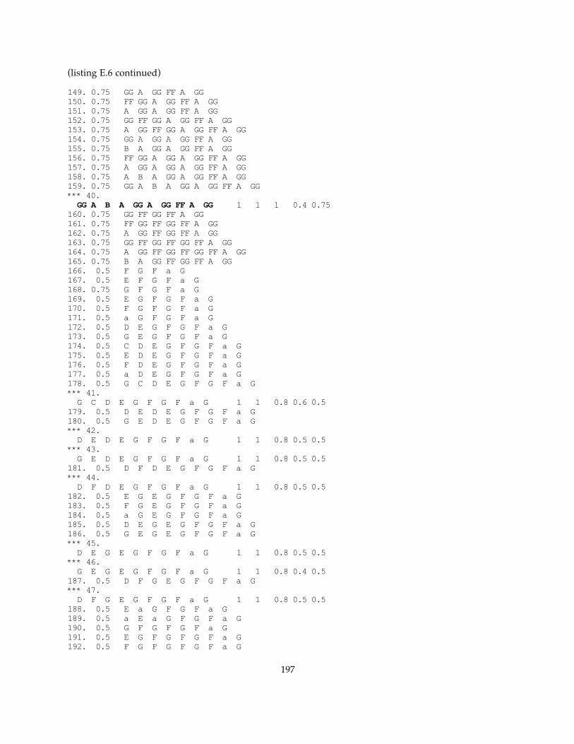
(listing E.6 continued)

149. 0.75 GG A GG FF A GG 150. 0.75 FF GG A GG FF A GG 151. 0.75 A GG A GG FF A GG 152. 0.75 GG FF GG A GG FF A GG 153. 0.75 A GG FF GG A GG FF A GG 154. 0.75 GG A GG A GG FF A GG 155. 0.75 B A GG A GG FF A GG 156. 0.75 FF GG A GG A GG FF A GG 157. 0.75 A GG A GG A GG FF A GG 158. 0.75 A B A GG A GG FF A GG 159. 0.75 GG A B A GG A GG FF A GG *** 40. GG A B A GG A GG FF A GG 1 1 1 0.4 0.75160. 0.75 GG FF GG FF A GG 161. 0.75 FF GG FF GG FF A GG 162. 0.75 A GG FF GG FF A GG 163. 0.75 GG FF GG FF GG FF A GG 164. 0.75 A GG FF GG FF GG FF A GG 165. 0.75 B A GG FF GG FF A GG 166. 0.5 F G F a G 167. 0.5 E F G F a G 168. 0.75 G F G F a G 169. 0.5 E G F G F a G 170. 0.5 F G F G F a G 171. 0.5 a G F G F a G 172. 0.5 D E G F G F a G 173. 0.5 G E G F G F a G 174. 0.5 C D E G F G F a G 175. 0.5 E D E G F G F a G 176. 0.5 F D E G F G F a G 177. 0.5 a D E G F G F a G 178. 0.5 G C D E G F G F a G *** 41. G C D E G F G F a G 1 1 0.8 0.6 0.5179. 0.5 D E D E G F G F a G 180. 0.5 G E D E G F G F a G *** 42. D E D E G F G F a G 1 1 0.8 0.5 0.5*** 43. G E D E G F G F a G 1 1 0.8 0.5 0.5181. 0.5 D F D E G F G F a G *** 44. D F D E G F G F a G 1 1 0.8 0.5 0.5182. 0.5 E G E G F G F a G 183. 0.5 F G E G F G F a G 184. 0.5 a G E G F G F a G 185. 0.5 D E G E G F G F a G 186. 0.5 G E G E G F G F a G *** 45. D E G E G F G F a G 1 1 0.8 0.5 0.5*** 46. G E G E G F G F a G 1 1 0.8 0.4 0.5187. 0.5 D F G E G F G F a G *** 47. D F G E G F G F a G 1 1 0.8 0.5 0.5188. 0.5 E a G F G F a G 189. 0.5 a E a G F G F a G 190. 0.5 G F G F G F a G 191. 0.5 E G F G F G F a G 192. 0.5 F G F G F G F a G

197

(listing E.6 continued)

193. 0.5 a G F G F G F a G 194. 0.5 D E G F G F G F a G 195. 0.5 G E G F G F G F a G *** 48. D E G F G F G F a G 1 1 0.8 0.5 0.5*** 49. G E G F G F G F a G 1 1 0.8 0.4 0.5196. 0.5 a E F G F a G 197. 0.5 D a E F G F a G 198. 0.5 E a E F G F a G 199. 0.5 G a E F G F a G 200. 0.5 C D a E F G F a G 201. 0.5 E D a E F G F a G 202. 0.5 F D a E F G F a G 203. 0.5 a D a E F G F a G 204. 0.5 E G a E F G F a G 205. 0.5 F G a E F G F a G 206. 0.5 a G a E F G F a G 207. 0.5 a E a E F G F a G 208. 0.5 aa g 209. 0.5 f aa g 210. 0.5 g f aa g 211. 0.25 e g f aa g 212. 0.5 f g f aa g 213. 0.25 aa g f aa g 214. 0.5 g f g f aa g 215. 0.5 e g f g f aa g 216. 0.5 aa g f g f aa g 217. 0.5 d e g f g f aa g 218. 0.5 g e g f g f aa g 219. 0.5 e d e g f g f aa g 220. 0.5 g d e g f g f aa g 221. 0.5 aa d e g f g f aa g 222. 0.5 d e d e g f g f aa g *** 50. d e d e g f g f aa g 1 1 0.8 0.5 0.5223. 0.5 d g d e g f g f aa g *** 51. d g d e g f g f aa g 1 1 0.8 0.5 0.5224. 0.5 e g e g f g f aa g 225. 0.5 aa g e g f g f aa g 226. 0.5 d e g e g f g f aa g *** 52. d e g e g f g f aa g 1 1 0.8 0.5 0.5227. 0.25 g aa g f aa g 228. 0.25 e g aa g f aa g 229. 0.25 aa g aa g f aa g 230. 0.25 d e g aa g f aa g 231. 0.25 g e g aa g f aa g 232. 0.25 e d e g aa g f aa g 233. 0.25 g d e g aa g f aa g 234. 0.25 aa d e g aa g f aa g 235. 0.25 e g e g aa g f aa g 236. 0.25 aa g e g aa g f aa g 237. 0.25 g aa g aa g f aa g 238. 0.25 e g aa g aa g f aa g 239. 0.25 aa g aa g aa g f aa g 240. 0.25 d e g f aa g 241. 0.25 e d e g f aa g 242. 0.25 g d e g f aa g

198

(listing E.6 continued)

243. 0.25 aa d e g f aa g 244. 0.25 d e d e g f aa g 245. 0.25 g e d e g f aa g 246. 0.25 e d e d e g f aa g 247. 0.25 g d e d e g f aa g 248. 0.25 aa d e d e g f aa g 249. 0.25 d e d e d e g f aa g *** 53. d e d e d e g f aa g 1 1 0.9 0.5 0.25250. 0.25 d g d e d e g f aa g *** 54. d g d e d e g f aa g 1 1 0.9 0.5 0.25251. 0.25 e g e d e g f aa g 252. 0.25 aa g e d e g f aa g 253. 0.25 d e g e d e g f aa g *** 55. d e g e d e g f aa g 1 1 0.9 0.5 0.25254. 0.25 d aa d e g f aa g 255. 0.25 g aa d e g f aa g 256. 0.25 e d aa d e g f aa g 257. 0.25 g d aa d e g f aa g 258. 0.25 aa d aa d e g f aa g 259. 0.25 e g aa d e g f aa g 260. 0.25 aa g aa d e g f aa g maxQSize: 15Priority queue size: 0chainedListPtrVector size: 0

Number of solutions: 55.

199

VITA

Nigel Gwee received a bachelor of music (piano) degree from the University of Western Australia in

1979. He came to the United States to pursue graduate studies and in 1989 completed a master of music

(voice) degree from Drake University, Iowa, and in 1998 a master of science (systems science) degree

from Louisiana State University, Baton Rouge.

In 1996, he received a doctoral degree in musicology from Louisiana State University. His

dissertation won the Josephine A. Roberts LSU Alumni Association Distinguished Dissertation Award

in the Arts, Humanities, and Social Sciences for the year of 1996.

200