CHAPTER 1

BASIC TOOLS

In which we meet the probability sample and the R language.

1.1 GOALS OF INFERENCE

1.1.1 Population or process?

The mathematical development for most of statistics is model-bused, and relies on specifying a probability model for the random process that generates the data. This can be a simple parametric model, such as a Normal distribution, or a complicated model incorporating many variables and allowing for dependence between observa- tions. To the extent that the model represents the process that generated the data, it is possible to draw conclusions that can be generalized to other situations where the same process operates. As the model can only ever be an approximation, it is important (but often difficult) to know what sort of departures from the model will invalidate the analysis.

Complex Surveys: A Guide to Analysis Using R. By Thomas Lumley Copyright @ 2010 John Wiley & Sons, Inc. 1

2 BASICTOOLS

The analysis of complex survey samples, in contrast, is usually design-based. The researcher specifies a population, whose data values are unknown but are regarded as fixed, not random. The observed sample is random because it depends on the random selection of individuals from this fixed population. The random selection procedure of individuals (the sample design) is under the control of the researcher, so all the probabilities involved can, in principle, be known precisely. The goal of the analysis is to estimate features of the fixed population, and design-based inference does not support generalizing the findings to other populations.

In some situations there is a clear distinction between population and process inference. The Bureau of Labor Statistics can analyze data from a sample of the US population to find out the distribution of income in men and women in the US. The use of statistical estimation here is precisely to generalize from a sample to the population from which it was taken.

The University of Washington can analyze data on its faculty salaries to provide evidence in a court case alleging gender discrimination. As the university’s data are complete there is no uncertainty about the distribution of salaries in men and women in this population. Statistical modelling is needed to decide whether the differences in salaries can be attributed to valid causes, in particular to differences in seniority, to changes over time in state funding, and to area of study. These are questions about the process that led to the salaries being the way they are.

In more complex analyses there can be something of a compromise between these goals of inference. A regression model fitted to blood pressure data measured on a sample from the US population will provide design-based conclusions about associations in the US population. Sometimes these design-based conclusions are exactly what is required, e.g., there is more hypertension in blacks than in whites. Often the goal is to find out why some people have high blood pressure: is the racial difference due to diet, or stress, or access to medical care, or might there be a genetic component?

1.1.2 Probability samples

The fundamental statistical concept in design-based inference is the probability sum- ple or random sample. In everyday speech, “taking a random sample” of 1000 individuals means a sampling procedure when any subset of 1000 people from the population is equally likely to be selected. The technical term for this is a “simple random sample”. The Law of Large Numbers implies that the sample of 1000 people is likely to be representative of the population, according to essentially any criteria we are interested in. If we compute the mean age, or the median income, or the proportion of registered Republican voters in the sample, the answer is likely to be close to the value for the population.

We could also end up with a sample of 1000 individuals from the US population, for example, by taking a simple random sample of 20 people from each state. On many criteria this sample is unlikely to be representative, because people from states with low populations are more likely to be sampled. Residents of these states have a similar age distribution to the country as a whole but tend to have lower incomes and

GOALS OF INFERENCE 3

be more politically conservative. As a result the mean age of the sample will be close to the mean age for the US population, but the median income is likely to be lower, and the proportion of registered Republican voters higher than for the US population. As long as we know the population of each state, this stratified random sample is still a probability sample. Yet another approach would be to choose a simple random sample of 50 counties from the US and then sample 20 people from each county. This sample would over-represent counties with low populations, which tend to be in rural areas. Even so, if we know all the counties in the US, and if we can find the number of households in the counties we choose, this is also a probability sample.

It is important to remember that what makes aprobability sample is the procedure for taking samples from a population, not just the data we happen to end up with.

The properties we need of a sampling method for design-based inference are as follows:

1. Every individual in the population must have a non-zero probability of ending up in the sample (written ni for individual i)

2. The probability ni must be known for every individual who does end up in the sample.

3. Every pair of individuals in the sample must have a non-zero probability of both ending up in the sample (written nij for the pair of individuals (i, j ) ) .

4. The probability nij must be known for every pair that does end up in the

The first two properties are necessary in order to get valid population estimates; the last two are necessary to work out the accuracy of the estimates. If individuals were sampled independently of each other the first two properties would guarantee the last two, since then nij = X i nj , but a design that sampled one random person from each US county would have ni > 0 for everyone in the US and nij = 0 for two people in the same county. In the survey package, as in most software for analysis of complex samples, the computer will work out nij from the design description, they do not need to be specified explicitly.

The world is imperfect in many ways, and the necessary properties are present only as approximations in real surveys. A list of residences for sampling will include some that are not inhabited and miss some that have been newly constructed. Some people (me, for example) do not have a landline telephone, others may not be at home or may refuse to answer some or all of the questions. We will initially ignore these problems, but aspects of them are addressed in Chapters 7 and 9.

sample.

1.1.3 Sampling weights

If we take a simple random sample of 3500 people from California (with total population 35 million) then any person in California has a 1/10000 chance of being sampled, so ni = 3500/3500000 = 1/10000 for every i. Each of the people we sample represents 10000 Californians. If it turns out that 400 of our sample have high

4 BASICTOOLS

blood pressure and 100 are unemployed, we would expect 400 x 10000 = 4 million people with high blood pressure and 100 x 10000 = 1 million unemployed in the whole state. If we sample 3500 people from Connecticut (population 3,500,000), all the sampling probabilities are equal to 3500/3500000 = 1/1000, so each person in the sample represents 1000 people in the population. If 400 of the sample had high blood pressure we would expect 400 x 1000 = 400000 people with high blood pressure in the state population.

The fundamental statistical idea behind all of design-based inference is that an individual sampled with a sampling probability of ni represents l/ni individuals in the population. The value l/ni is called the sampling weight.

This weighting or “grossing up” operation is easy to grasp for a simple random sample where the probabilities are the same for every one. It is less obvious that the same rule applies when the sampling probabilities can be different. In particular, it may not be intuitive that the sampling probabilities for individuals who were not sampled do not need to be known.

Consider measuring income on a sample of one individual from a population of N , where ni might be different for each individual. The estimate (fincome) of the total income of the population (Tincome) would be the income for that individual multiplied by the sampling weight:

1 Tincome = - x incomei.

ni

This will not be a very good estimate, since it is based on only one person, but it will be unbiased: the expected value of the estimate will equal the true population total. The expected value of the estimate is the value of the estimate when we select person i, times the probability of selecting person i , added up over all people in the population

N

= C i n c o m e i

= Tincome. i=l

The same algebra applies with only slightly more work to samples of any size. The l/ni sampling weights used to construct the estimate cancel out the xj probability that this particular individual is sampled. The estimator of the population total is called the Horvitz-Thompson estimator [63] after the authors who proposed the most general form and a standard error estimate for it, but the principle is much older.

Estimates for any other population quantity are derived in various ways from estimates for a population total, so the Horvitz-Thompson estimator of the population total is the foundation for all the analyses described in the rest of the book. Because of the importance of sampling weights and the inconvenience of writing fractions it

GOALS OF INFERENCE 5

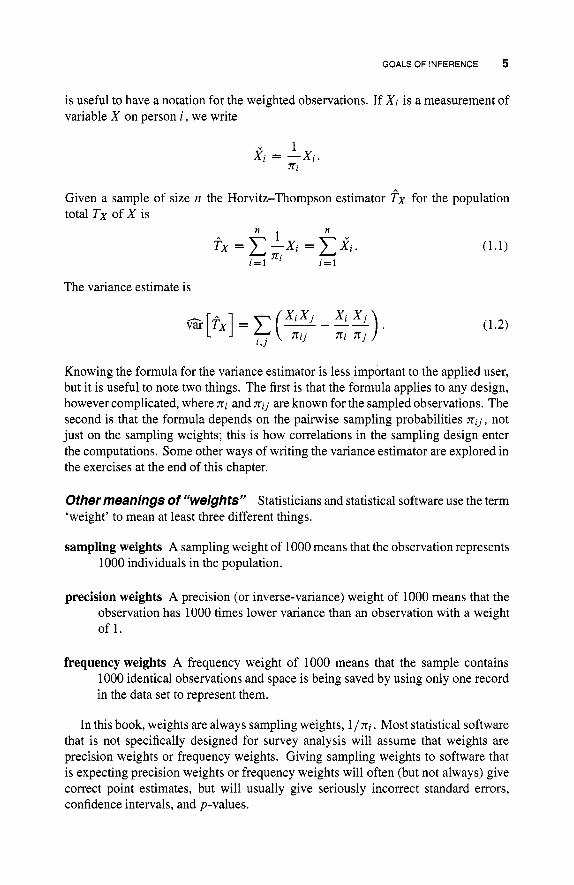
is useful to have a notation for the weighted observations. If X i is a measurement of variable X on person i, we write

Given a sample of size y1 the Horvitz-Thompson estimator fx for the population total Tx of X is

n

The variance estimate is

Knowing the formula for the variance estimator is less important to the applied user, but it is useful to note two things. The first is that the formula applies to any design, however complicated, where ni and n i j are known for the sampled observations. The second is that the formula depends on the pairwise sampling probabilities njj , not just on the sampling weights; this is how correlations in the sampling design enter the computations. Some other ways of writing the variance estimator are explored in the exercises at the end of this chapter.

Other meanings of “weights” Statisticians and statistical software use the term ‘weight’ to mean at least three different things.

sampling weights A sampling weight of 1000 means that the observation represents 1000 individuals in the population.

precision weights A precision (or inverse-variance) weight of 1000 means that the observation has 1000 times lower variance than an observation with a weight of 1.

frequency weights A frequency weight of 1000 means that the sample contains 1000 identical observations and space is being saved by using only one record in the data set to represent them.

In this book, weights are always sampling weights, l/nj. Most statistical software that is not specifically designed for survey analysis will assume that weights are precision weights or frequency weights. Giving sampling weights to software that is expecting precision weights or frequency weights will often (but not always) give correct point estimates, but will usually give seriously incorrect standard errors, confidence intervals, and p-values.

6 BASICTOOLS

1.1.4 Design effects

A complex survey will not have the same standard errors for estimates as a simple random sample of the same size, but many sample size calculations are only conve- niently available for simple random samples. The design effect was defined by Kish (1965) as the ratio of a variance of an estimate in a complex sample to the variance of the same estimate in a simple random sample [75].

If the necessary sample size for a given level of precision is known for a simple random sample, the sample size for a complex design can be obtained by multiplying by the design effect. While the design effect will not be known in advance, some useful guidance can be obtained by looking at design effects reported for other similar surveys.

Design effects for large studies are usually greater than 1 .O, implying that larger sample sizes are needed for complex designs than for a simple random sample. For example, the California Health Interview Survey reports typical design effects in the range 1.4-2.0. It may be surprising that complex designs are used if they require both larger samples sizes and special statistical methods, but as Chapter 3 discusses, the increased sample size can often still result in a lower cost.

The other ratio of variances that is of interest is the ratio of the variance of a correct estimate to the incorrect variance that would be obtained by pretending that the data are a simple random sample. This ratio allows the results of an analysis to be (approximately) corrected if software is not available to account for the complex design. This second ratio is sometimes called the design effect and sometimes the misspecification effect.

That is, the design effect compares the variance from correct estimates in two different designs, while the misspecification effect compares correct and incorrect analyses of the same design. Although these two ratios of variances are not the same, they are often similar for practical designs. The misspecification effect is of relatively little interest now that software for complex designs is widely available, and it will not appear further in this book.

1.2 AN INTRODUCTION TO THE DATA

Most of the examples used in this book will be based either on real surveys or on simulated surveys drawn from real populations. Some of the data sets will be quite large by textbook standards, but the computer used to write this book is a laptop dating from 2006, so it seems safe to assume that most readers will have access to at least this level of computer power. Links to the source and documentation for all these data sets can be found on the web site for the book.

Nearly all the data are available to you in electronic form to reproduce these analyses, but some effort may be required to get them. Surveys in the United States tend to provide (non-identifying, anonymized) data for download by anyone, and the datasets from these surveys used in this book are available on the book’s web site in directly usable formats. Access to survey data from Britain tends to require much filling in of forms, so the book’s web site provides instructions on where

AN INTRODUCTION TO THE DATA 7

to find the data and how to convert it to usable form. These national differences partly reflect the differences in copyright policy in the two countries. In the US, the federal government places materials created at public expense in the public domain; in Britain, the copyright is retained by the government.

You may be unfamiliar with some of the terminology in the descriptions of data sets, which will be described in subsequent chapters.

1.2.1 Real surveys

NHANES. The National Health and Nutrition Examination Surveys have been conducted by the US National Center for Health Statistics (NCHS) since 1970. They are designed to provide nationwide data on health and disease, and on dietary and clinical risk factors. Each four-year cycle of NHANES recruits about 28000 people in a multistage sample. These participants receive an interview and a clinical exam, and have blood samples taken. Several hundred data variables are available in the public use data sets.

FRS. The Family Resources Survey collects information on the incomes and cir- cumstances of private households in the United Kingdom. It was designed to collect information needed by the Department for Work and Pensions. The survey first sam- ples 1848 postcode sectors from Great Britain, stratified by geographic region and by some employment and income variables. The postcode sectors are sampled with probability proportional to the number of mailing addresses with fewer than 50 mail items per day, an estimate of the number of households. Within each postcode sector a simple random sample of households is taken. A few variables from the Scottish subset of FRS have been made available by the PEAS project at Napier University (aftel some modification to p~otec‘i anonymity).

NHIS. The National Health Interview Survey, conducted by the National Center for Health Statistics is the oldest of the major health-related surveys in the United States. The National Health Survey Act (1956) provided “for a continuing survey and special studies to secure accurate and current statistical information on the amount, distribution, and effects of illness and disability in the United States and the services rendered for or because of such conditions.” NHIS plans to sample about 35000 households, containing about 87500 people, each year, but the survey is designed so that the results will still be useful if the sampling has to be curtailed because of budget shortfalls, as happened in 2006 and 2007. NHIS, unlike NHANES, is restricted to self-reported information and does not make clinical or biological measurements on participants. NHIS was the first major survey to include instructions for analysis using R.

SIP/? The Survey of Income and Program Participation is a series of panel surveys conducted by the US Census Bureau, with panels of US households recruited in a multistage sampling design. The sample size has varied from about 14000 to about 37000 households. SIPP asks questions about income and about participation

8 BASICTOOLS

in government support programs such as food stamps. The same households are repeatedly surveyed over time to allow economic changes to be measured more accurately.

CHIS. The California Health Interview Survey samples households from California by random-digit dialing within geographic regions. The survey is conducted every two years and samples 40000-50000 households. Unlike the surveys above, which are conducted by government agencies, CHIS is conducted by the Center for Health Policy Research at the University of California, Los Angeles. CHIS asks questions about health, risk factors for disease, health insurance, and access to health care.

SHS. The Scottish Household Survey interviews about 3 1000 households every two years. Individual households are sampled in densely populated areas of Scotland; in the rest of the country a two-stage sample is used. The first stage samples census enumeration districts, which contain an average of 150 households, then the second stage samples households within these districts. The survey covers a wide range of topics such as housing, income, transport, and social services. Data from a subset of variables has been made generally available (after some further modification to protect anonymity) by the PEAS project at Napier University.

BRFSS. The Behavioral Risk Factor Surveillance System is a telephone survey of behavioral risk factors for disease. The survey is conducted by most US states using materials supplied by the National Center for Health Statistics. The number of states involved has increased from 15 in 1984 to all 50 in 2007 (plus the District of Columbia, Guam, Puerto Rico, and the US Virgin Islands) and the sample size from 12000 to 430000. It is now the world’s largest telephone survey.

1.2.2 Populations

Evaluating and comparing analysis methods requires realistic data where the true answer is known. We will use some complete population data to create artificial probability samples, and compare the results of our analyses to the population values. Population data are also useful for illustrating design and preprocessing calculations that are done before the survey data reach the public use files.

Election data. Voting data for the US presidential elections is available for each county. We will try to predict the result from samples of the data and use the voting data from previous elections to improve predictions.

NWTS. Wilms’ tumor is a rare childhood cancer of the kidney, curable in about 90% of cases. Most children in the United States with Wilms’ tumor participate in randomized clinical trials conducted by the National Wilms’ Tumor Study Group. Data from these studies [54,38] has been used extensively in research on two-phase epidemiological studies by Norman Breslow and co-workers, and some of this data

OBTAINING THE SOiTWARE 9

is now publically available. In our analyses the focus is on estimating the risk of relapse after initially successful treatment.

Crime in Washington. The Washington Association of Sheriffs and Police Chiefs collects data on crimes reported to police in Washington (the state, not the city). The data are reported broken down by police district and by type of crime.

API. The California Academic Performance Index is computed from standardized tests administered to students in California schools. In addition to academic per- formance data for the schools there are a wide range of socio-economic variables available. These data have been used extensively to illustrate the use of survey soft- ware by Academic Computing Services at the University of California, Los Angeles.

PBC. Primary biliary cirrhosis is a very rare liver disease that is treatable only by transplantation. Before transplantation was available, the Mayo Clinic conducted a randomized trial of what turned out to be a completely ineffective treatment. The data from 312 participants in the trial and 106 patients who did not participate was used to create a model for predicting survival that is still used in scheduling liver transplants. As the Mayo Clinic was a major center for treatment of primary biliary cirrhosis these 41 8 patients represent essentially the entire population in the nearby states. The de-identified public version of the dataset was created by Terry Therneau in conjunction with his development of software for survival analysis. It has become a standard teaching and research example.

1.3 OBTAINING THE SOFTWARE

R is probably the most widely used software for statistical research and for distributing new statistical methods. The design of R is based closely on Bell Labs’ S, one of the first systems for interactive statistical computing. John Chambers, the main designer of S, received the Software Systems Award from the Association for Computing Machinery

For the S system, which has forever altered how people analyze, visualize, and manipulate data.

The drawback is, of course, that users of S and R have to alter how they analyze, visualize, and manipulate data; the learning curve may sometimes be steep. R does not have a point-and-click GUI interface, and the programming is more flexible but also more complex than the macro languages of most statistical packages.

Although all the code needed to do analyses will be presented in this book, it is not all explained in detail and readers who are not familiar with R would benefit from reading an introductory book on the language. A comprehensive list of books on R is given on the R Project web page. Fox [47] is written for social scientists and Dalgaard [37] for health scientists. Chambers [32] covers more advanced programming and design philosophy for R code.

10 BASIC TOOLS

1.3.1 Obtaining R

Windows or Macintosh users can download R from the Comprehensive R Archive Network (CRAN) at the central site, h t t p : / / c r a n . r - p r o j e c t . org, or at one of many mirror sites around the world ( h t t p : / / c r a n . r - p r o j e c t . org/mirrors . html. Most Linux distributions provide precompiled versions of R through their package systems, and users on other Unix and Unix-like systems can easily compile R from the source code available from CRAN. New versions of R come out frequently, and you should update your installation at least once a year.

System adminstrators installing R for multiple users, or people wishing to compile R from the source code, should read the R Installation and Administration manual available on CRAN.

1.3.2 Obtaining the survey package

An important feature of R is the huge collection of add-on packages written by users, with the number of available packages doubling about every 18 months. In particular, R itself has no features for design-based inference and survey analysis; all the analysis features in this book come from the survey package (Lumley [99, loll).

These packages can most easily be installed from inside R, using the Packages menu on the Windows version of R, or the Packages & Data menu on the Macintosh version. Some chapters in this book also make use of other add-on packages for graphics, imputation, and database access. These will be installed in the same way. When you use a contributed R package for published research, please cite the package (as journal policies permit). The c i t a t i o n 0 function shows the preferred citation for a package or generates a default one if the author has not specified.

The examples in this book used version 3.10-1 of the survey package and were run in R version 2.7.2. The home page for the survey package ( h t t p : / / f a c u l t y . washingt on. edu/ t lumley/survey) will have information about any changes for newer versions of the package as they are released. Nearly all code should continue to run without modification, but there are likely to be small changes in the formatting of output.

1.4 USING R

This section provides a brief overview of getting data into R and doing some simple computations. Further introductory material on R can be found in Appendix B.

1.4.1 Reading plain text data

The simplest format for plain text data has one record per line with variable names in the first line of the file, with variables separated by commas. Files with this structure often have names ending . csv. Most statistical packages and databases can easily export data as comma-separated text.

> nwts <- read. csv("C:/svybook/nwts/nwts-share. csvl') > summary(nwts)

t r e l t sur r e l a p s Min. : 0,01095 Min. : 0.01095 Min. :O.OOOO 1st Qu.: 4.94182 1st Qu.: 6.24093 1st qu.:O.OOOO Median : 9.77139 Median :10.36003 Median :O.OOOO Mean : 9.64874 Mean :10.32634 Mean :0.1709 3rd Qu.:14.01095 3rd qu.:14.42847 3rd Qu.:O.OOOO Max. :22.50240 Max. :22.50240 Max. :1.0000 [ . . . output t runca ted . . . ] > head (nwt s)

t s u r r e l aps dead study s tage unfav.pat unfavO 1 21.88090 21.88090 0 0 3 I I 1 2 11.28268 11.28268 0 0 3 2 0 0 3 22.11362 22.11362 0 0 3 1 I I 4 8.02464 8.02464 0 0 3 2 0 0 5 20.49829 20.49829 0 0 3 2 0 0 6 14.39562 14.39562 I 1 3 2 0 1 I... output t runca ted . . . 1 > names(nwts)

t r e l

11 t r e 1 ' I t s u r I( 'I r e 1 aps II dead 'I If study I' [SI st age" "unf av . pa t It "unf avo" age 'I "yr , r eg i s "

[Ill "specwgt" "tumdian" > nrowhwts) [ I 1 3915 > ncol(nwts) 111 12

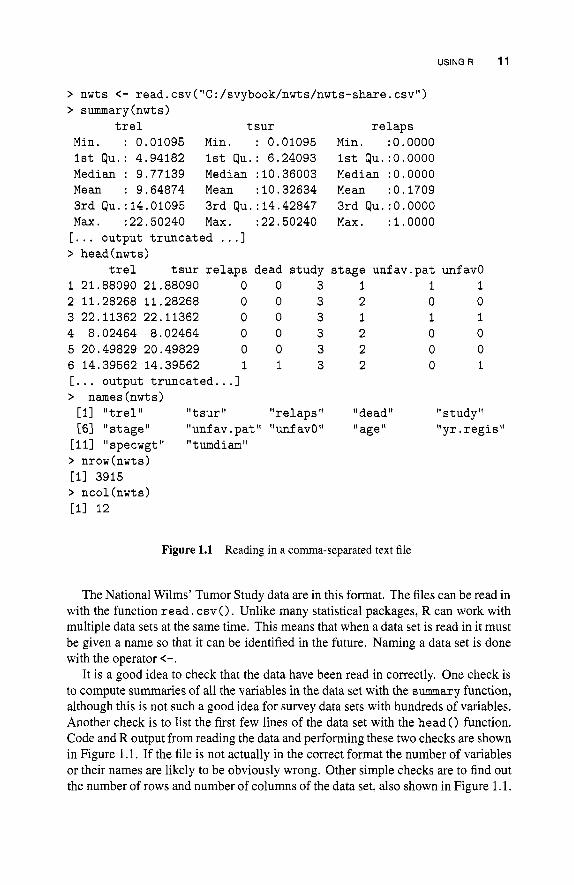
Figure 1.1 Reading in a comma-separated text file

The National Wilms' Tumor Study data are in this format. The files can be read in with the function read . csv () . Unlike many statistical packages, R can work with multiple data sets at the same time. This means that when a data set is read in it must be given a name so that it can be identified in the future. Naming a data set is done with the operator <-.

It is a good idea to check that the data have been read in correctly. One check is to compute summaries of all the variables in the data set with the summary function, although this is not such a good idea for survey data sets with hundreds of variables. Another check is to list the first few lines of the data set with the h e a d o function. Code and R output from reading the data and performing these two checks are shown in Figure 1.1, If the file is not actually in the correct format the number of variables or their names are likely to be obviously wrong. Other simple checks are to find out the number of rows and number of columns of the data set, also shown in Figure 1.1.

12 BASIC TOOLS

The > notation at the beginning of each line is the R prompt, not part of the code to be entered. If this prompt changes to a + sign, it means that R is waiting for the line of input to be finished, which may indicate that parentheses or quotation marks have been left open on the previous line. The "Escape" key will cancel the incomplete line of input. In the examples in this book the prompt will only be shown in transcripts that include R output; examples of R code without output will omit the prompt.

1.4.2 Reading data from other packages

R can read data saved in binary formats from SPSS and Stata, and the format produced by PROC XPORT in SAS. NHANES data are now distributed in the PROC XPORT format, as are data from BRFSS. The Inter-University Consortium for Political and Social Research (ICPSR) and the SodaPop archive at Pennsylvania State University often provide data sets in Stata and SPSS formats, saving the effort needed to construct variable names and value labels for data read in as plain text.

The R functions for reading data in these formats are in the foreign package. This package is part of the R distribution, but is not automatically loaded into memory when R starts. To load the package from the package library, type

library(f oreign)

When the package is loaded all its functions and help pages become available. The functions readexport 0, read.dta0, and read.spss0 will read SAS XPORT, Stata, and SPSS files, respectively. These functions take a file name as the first argument, and read. d t a O and read. spss 0 have other options that control the handling of dates and factors.

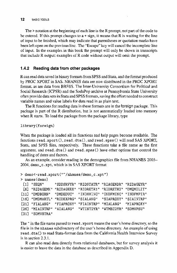
As an example, consider reading in the demographics file from NHANES 2003- 2004, demo-c . xpt, which is in SAS XPORT format

> demo<-read.xport (""/nhanes/demo-c.xpt") > names (demo) [I] IISEQN" "SDDSRVYR" "RIDSTATR" "RIAGENDR" "RIDAGEYR" [ 61 'I RID AGEMN I' 'I RID AGEEX I' I' RIDRETHI I' I' RIDRETH2 'I I' DMQMILIT I'

[ll] "DMDBORN" "DMDEDUC" I' INDHHINC" "INDFMINC" "INDFMPIR" [I61 "DMDMARTL" "RIDEXPRG" "SIALANG" "SIAPROXY" "SIAINTRP" [2 11 I' FI ALANG 'I I' FI APROXY 'I 'I FI AINTRP I' 'I MI ALANG 'I "MIAPROXY I' [261 "MIAINTRP" "AIALANG" "WTINT2YR" "WTMEC2YR" "SDMVPSU" [3 11 I' SDMVSTRA"

The " in the file name passed to read. xport means the user's home directory, so the file is in the nhanes subdirectory of the user's home directory. An example of using read. dtaO to read Stata-format data from the California Health Interview Survey is in section 2.3.1.

R can also read data directly from relational databases, but for survey analysis it is easier to leave the data in the database as described in Appendix D.

USING R 13

1.4.3 Simple computations

Since more than one data set can be loaded at a time, referring to a variable requires saying which data set it is in. The demo-c . xpt data set from NHANES that was loaded above is called demo, so the age variable RIDAGEYR is called demo$RIDAGEYR. The $ is like the possessive “’s”; demo$RIDAGEYR is demo’s RIDAGEYR variable.

Subsets of a variable can be indicated by

0 Positive numbers: demo$RIDAGEYR [lo0 : 1501 is observations 100 to 150 of the variable.

0 Negative numbers: demo$RIDAGEYR [-c (1 : 10, 100 : IOOO)] is all the ob- servations except 1 to 10 and 100 to 1000. The function c 0 collects its arguments into a single vector.

0 Logical (TRUUFALSE) vectors: demo$RIDAGEYR [demo$RIAGENDR==ll are the ages of the men (RIAGENDR is gender). Note the use of == rather than just = for testing equality.

The repeated use of $ in the same expression can become tedious, and the example for logical subsets can be written more compactly as

with(demo , RIDAGEYR [RIAGENDR==I] )

where with (1 specifies a particular data set as the default place to look up variables. The $ notation allows single variables to be specified, but it is also necessary to refer

to groups of variables. In the example in section 2.3.1, chis-adult [,420:4991 refers to columns 420 to 499 of the California Health Interview Survey adult data set. A data set can be subscripted in both rows and columns: the numbers before the comma indicate rows and the numbers after the comma indicate columns, following the usual matrix notation in mathematics. Omitting the number before the comma means that all rows are used, and all columns when the number after the comma is omitted. Subsets of a data set can also be constructed with the subset 0 function, for example, kids <- subset (demo, RIDAGEYR < 18). Variables in the subset expression will first be searched for in the data set, the $ notation is not needed.

New variables can be created in a data set with the same $ notation. For example, to create a variable indicating age less than 18

demo$underl8 <- demo$RIDAGEYR < 18

Missing data. Missing data are indicated by NA. It is useful to think of this as “Don’t Know”, so that l+NA is NA, NA==2 is NA, and even NA==NA is NA (to test for NA use is .naO). Simple statistical functions such as mean(>, s d 0 , andmedian0 give NA as the result if any of their input data are missing: if you don’t know the numbers, you don’t know the average. These functions have an option na . rm=TRUE to ask for the missing values to be omitted.

It will often be necessary to recode values such as -9 to NA before analysis, e.g.,

pbc[pbc$trt == -91 <- NA

14 BASIC TOOLS

EXERCISES

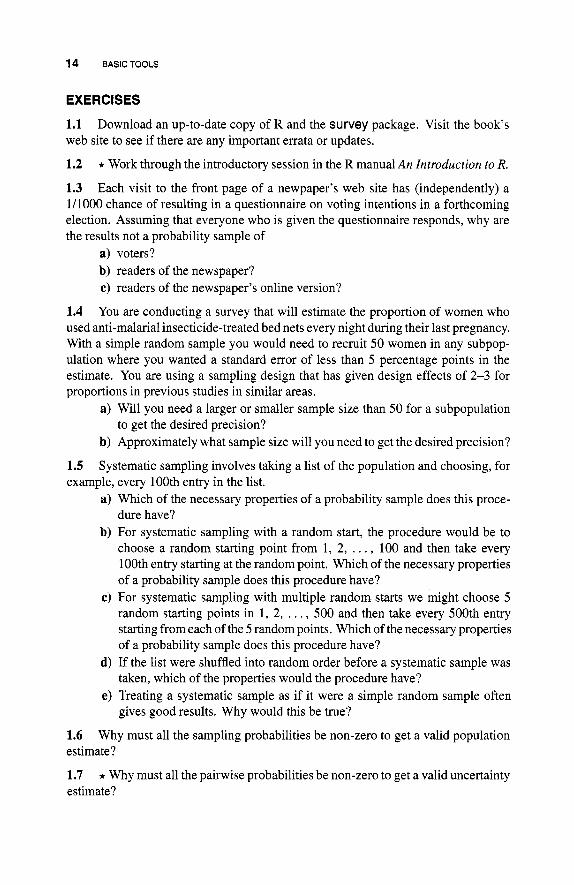
1.1 Download an up-to-date copy of R and the survey package. Visit the book’s web site to see if there are any important errata or updates.

1.2 * Work through the introductory session in the R manual An Introduction to R.

1.3 Each visit to the front page of a newpaper’s web site has (independently) a 1/1000 chance of resulting in a questionnaire on voting intentions in a forthcoming election. Assuming that everyone who is given the questionnaire responds, why are the results not a probability sample of

a) voters? b) readers of the newspaper? c) readers of the newspaper’s online version?

1.4 You are conducting a survey that will estimate the proportion of women who used anti-malarial insecticide-treated bed nets every night during their last pregnancy. With a simple random sample you would need to recruit 50 women in any subpop- ulation where you wanted a standard error of less than 5 percentage points in the estimate. You are using a sampling design that has given design effects of 2-3 for proportions in previous studies in similar areas.

a) Will you need a larger or smaller sample size than 50 for a subpopulation to get the desired precision?

b) Approximately what sample size will you need to get the desired precision?

Systematic sampling involves taking a list of the population and choosing, for

a) Which of the necessary properties of a probability sample does this proce- dure have?

b) For systematic sampling with a random start, the procedure would be to choose a random starting point from 1, 2, . . . , 100 and then take every 100th entry starting at the random point. Which of the necessary properties of a probability sample does this procedure have?

c) For systematic sampling with multiple random starts we might choose 5 random starting points in 1, 2, . . . , 500 and then take every 500th entry starting from each of the 5 random points. Which of the necessary properties of a probability sample does this procedure have?

d) If the list were shuffled into random order before a systematic sample was taken, which of the properties would the procedure have?

e) Treating a systematic sample as if it were a simple random sample often gives good results. Why would this be true?

Why must all the sampling probabilities be non-zero to get a valid population

* Why must all the painvise probabilities be non-zero to get a valid uncertainty

1.5 example, every 100th entry in the list.

1.6 estimate?

1.7 estimate?

EXERCISES 15

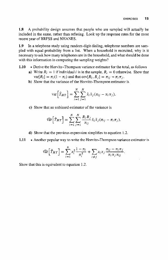
1.8 A probability design assumes that people who are sampled will actually be included in the same, rather than refusing. Look up the response rates for the most recent year of BRFSS and NHANES.

1.9 In a telephone study using random-digit dialing, telephone numbers are sam- pled with equal probability from a list. When a household is recruited, why is it necessary to ask how many telephones are in the household, and what should be done with this information in computing the sampling weights?

1.10 * Derive the Horvitz-Thompson variance estimator for the total, as follows a) Write Ri = 1 if individual i is in the sample, Ri = 0 otherwise. Show that

b) Show that the variance of the Horvitz-Thompson estimator is var[Ri] = n i ( l - X i ) and that COV[R~, R j ] = nij - ninj.

c) Show that an unbiased estimator of the variance is

d) Show that the previous expression simplifies to equation 1.2.

1.11 * Another popular way to write the Horvitz-Thompson variance estimator is

Show that this is equivalent to equation 1.2.