Complex Shallow Water Simulations throughLattice-Boltzmann-based Mesoscopic NumericalTreatment Exploiting Hybrid Compute Nodes

Markus Geveler

Institut fur Angewandte MathematikTU Dortmund, Germany

markus.geveler@math.tu-dortmund.de

GS11Shallow Water Simulations on GPUs

Long Beach, March 23, 2011

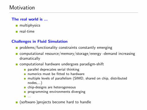
Motivation

The real world is ...

multiphysics

real-time

Challenges in Fluid Simulation

problems/functionality constraints constantly emerging

computational resource/memory/storage/energy -demand increasingdramatically

computational hardware undergoes paradigm-shift

parallel deprecates serial thinkingnumerics must be fitted to hardwaremultiple levels of parallelism (SIMD, shared on chip, distributednodes,...)chip-designs are heterogeneousprogramming environments diverging...

(software-)projects become hard to handle

Motivation

When speaking of compute nodes...

1-8 GB/s

PCIe

1-2 GB/s

Infiniband (PCIe)

CPU-Socket

cores

caches

6-35 GB/s

Host Memory

20-180 GB/s

GPU

DeviceMemory

cores

caches

...

SIM

T-M

P

SIM

T-M

P

shared caches and MCs

...

... SIM

T-M

P

SIM

T-M

P

Motivation

Simplification

using SWE is a simplification on the model-level

other levels:

numerical method(s)computational accuracy

Modification on the discrete and model levels and adjustment tohardware

pure macroscopic approach: modification on the PDE-level →discretisation

pure microscopic approach: modification on discrete-level →reconstruct continuum

LBM is mesoscopic: allows both

LBM for SWE

Discrete phase space, general form of LBM: collision and streaming

eα =

(0, 0) α = 0

e(cos (α−1)π4 , sin (α−1)π

4 ) α = 1, 3, 5, 7√2e(cos (α−1)π

4 , sin (α−1)π4 ) α = 2, 4, 6, 8,

The LBE

fα(x + eα∆t, t+ ∆t) = fα(x, t) +Q(fα, fβ), β = 1, ..., k .

LBM for SWE

Collision operator

f tempα (x, t) = fα(x, t)− 1

τ(fα − feqα )

Equilibrium distribution for Shallow Water Equations

f eqα =

h(1− 5gh

6e2 −2

3e2uiui) α = 0

h( gh6e2 + eαiui3e2 +

eαjuiuj2e4 − uiui

6e2 ) α = 1, 3, 5, 7

h( gh24e2 + eαiui

12e2 +eαjuiuj

8e4 − uiui24e2 ) α = 2, 4, 6, 8

Physical quantities

h(x, t) =∑α

fα(x, t) and ui(x, t) =1

h(x, t)

∑α

eαifα,

→ dry states?

Boundary conditions

Simple bounce-back

Accuracy

LBM in general: 2nd order in space, 2nd order in time

bounce back gives 1st order in space for boundary sites

often: porous media, non-axis-aligned geometry → sufficient?

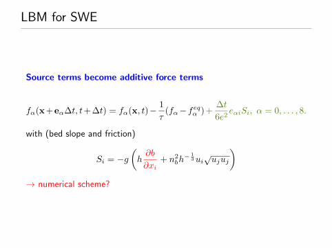
LBM for SWE

Source terms become additive force terms

fα(x+eα∆t, t+∆t) = fα(x, t)− 1

τ(fα−feqα )+

∆t

6e2eαiSi, α = 0, . . . , 8.

with (bed slope and friction)

Si = −g(h∂b

∂xi+ n2bh

− 13ui√ujuj

)→ numerical scheme?

SWE with FSI

Idea Ingredients

moving boundaries

fluid initialisation

momentum exchange

dynamic lattice → implementation

SWE with FSI

Boundary conditions for moving boundary: BFL

f temp−β (x, t+ ∆t) = C1(q)fβ(x, t) + C2(q)fβ(x + e−β , t) + C3(q)f−β(x, t)+

C4(q)2∆xw−βc−2s [uB(bβ) · e−β ],

quality-down: q = 1/2⇒

f temp−β (x, t+ ∆t) = 6∆x w−β(uB(bβ) · e−β).

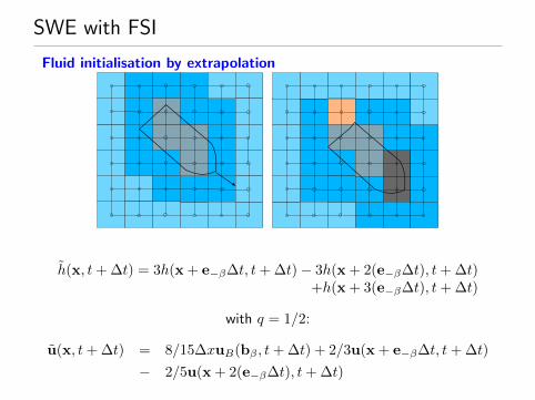
SWE with FSI

Fluid initialisation by extrapolation

h(x, t+ ∆t) = 3h(x + e−β∆t, t+ ∆t)− 3h(x + 2(e−β∆t), t+ ∆t)+h(x + 3(e−β∆t), t+ ∆t)

with q = 1/2:

u(x, t+ ∆t) = 8/15∆xuB(bβ , t+ ∆t) + 2/3u(x + e−β∆t, t+ ∆t)

− 2/5u(x + 2(e−β∆t), t+ ∆t)

SWE with FSI

Momentum Exchange Algorithm

fMEA−β (b, t) = eβi(f

tempβ (x, t) + f temp

−β (x, t+ ∆t)).

The forces can be aggregated into the total force acting on b:

F (b, t) =∑α

fMEAα (b, t).

x

q

u b

MEA

b

Implementation: A word on HPC software

HONEI

primary design goals: abstract from target-hardware, exploit allresources in a node

support natively:x86 SIMD (handcrafted SSE2 using intrinsics)x86 multi-core (pthreads)distributed memory clusters (MPI)NVIDIA GPUs (CUDA 3) + multiple GPUs + hybrid computationsCell BE (libspe2)

unittest + benchmark frameworks, visualisation

build system to create SPE kernels for Cell BE, CUDA-kernels

thread-management, MPI

support for RTTI and exception-handling, memory transfers

RPC system to call SPE programs from the PPE

templates to facilitate development of new callable SPE functionsand registering them with the RPC system

automatic job scheduling

...

Implementation: packed lattice

One datastructure fits all

compress lattice: stationary obstacles

store contiguously in memory

instationary obstacles (moving solids): colouring

cut domain in one dimension

patch 0 patch 1

Implementation: GPU

Shared memory: general

cache lattice velocities eαi

Memory arbitration

external device memory management

works ’behind the scenes’

transfers only if necessary

Complex kernels (force, FSI)

avoid branch-divergence

cache factors in force terms

cache extrapolation weights

Implementation: Inhomogeneous SWE

Dry-states

1 define fluid sites with h < ε as dry: h← 0, ui ← 0

2 confine local oscillations:

φU (x) = max(−U,min(U, x))

Centred scheme for slope term

Si = Si(x, t) insufficient, Si = Si(x+1

2eα∆t, t+∆t) prohibitively expensive!

Solution: Si = Si(x + 12eα∆t, t) ([Zhou 2004])

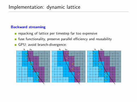
Implementation: dynamic lattice

Backward streaming

repacking of lattice per timestep far too expensive

fuse functionality, preserve parallel efficiency and reusability

GPU: avoid branch-divergence:

Implementation: hybrid compute nodes

Composition of hybrid solver: example

3 patches of domain initially

1 patch subdivided for the MultiCore backend

each of the four MC-threads use the SSE backend

resulting in utilisation of two GPUs and all cores of the (quadcore)CPU

Hybrid LBM Solver

GPU::CUDA GPU::CUDA CPU::MultiCore::SSE

CPU::SSE CPU::SSE CPU::SSE CPU::SSE

Results

Numerical properties

approved: manydifferent simulations

well suited for CG

finding solverparameters is hard

timestep usually small

stabilisation stillexperimental

Results

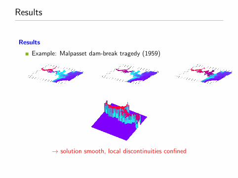
Method even works for ’real-world’ problems

Example: Malpasset, France - arch dam-break tragedy (1959): 451kills, ˜$70 M worth of damage

Results

Results

Example: Malpasset dam-break tragedy (1959)

→ solution smooth, local discontinuities confined

Results

Performance: core i7 Gulftown 980 X, 3.33GHz Hexacore + 2 ×FERMI (Tesla C2070)

0

50

100

150

200

250

300

40 K 4 M 16 M

MF

LU

PS

#lattice-sites

SSE, 1threadSSE, 6 threadsGPU, 2 devicesGPU, 1 device

HYBRID GPU, 1 device, SSE, 6 threadsHYBRID GPU, 2 devices, SSE, 6 threads

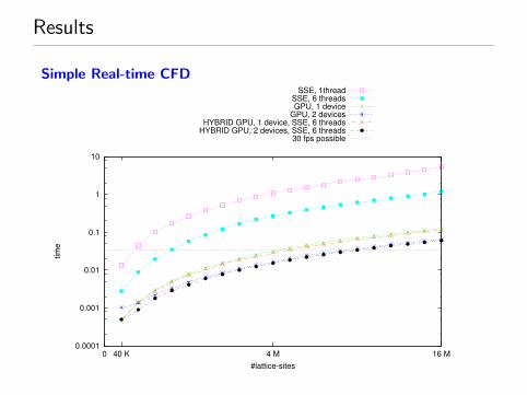
Results

Simple Real-time CFD

0.0001

0.001

0.01

0.1

1

10

0 40 K 4 M 16 M

tim

e

#lattice-sites

SSE, 1threadSSE, 6 threadsGPU, 1 device

GPU, 2 devicesHYBRID GPU, 1 device, SSE, 6 threads

HYBRID GPU, 2 devices, SSE, 6 threads30 fps possible

Conclusions

Real-time and beyond

LBM well suited for multi-level parallelism due to data locality

up to 9 M lattice sites in real time possible (30 fps)

Malpasset dam break simulation running at 1,100 fps

GPU + CPU works well, only for very small problems →synchronisation too expensive

Remarks

basic LB-methods easy to implement, extend, maintain, ...

very sophisticated HPC LBM codes available → www.skalb.de

Acknowledgements

Supported by BMBF, HPC Software fur skalierbare Parallelrechner: SKALBproject 01IH08003D.

Thanks to Dirk Ribbrock and all contributors to HONEI. Thanks to RRZE forhardware access.