Complex Dynamics in Winner-Take-All Neural Nets …bard/bardware/papers/wta-92.pdfComplex Dynamics in Winner-Take-All Neural Nets With Slow Inhibition BARD ERMENTROUT* University of

NeuralNetworks, Vol. 5, pp. 415--431, 1992 0893-6080/92 $5.00 + .00 Printed in the USA. All rights reserved. Copyright © 1992 Pergamon Press Ltd.

ORIGINAL CONTRIBUTION

Complex Dynamics in Winner-Take-All Neural Nets With Slow Inhibition

BARD E R M E N T R O U T *

University of Pittsburgh

(Received 13 December 1990; revised and accepted 8 October 1991 )

Abstract--We consider a layer of excitatory neurons with small asymmetric excitatory connections and strong coupling to a single inhibitory interneuron. I f the inhibition is fast, the network behaves as a winner-take-all network in which one cell fires at the expense of all others. As the inhibition slows down, oscillatory behavior begins. This is followed by a symmetric rotating solution in which neurons share the activity in a round-robin fashion. Finally, i f the inhibition is sufficiently slower than excitation the neurons completely synchronize to a global periodic solution. Conditions guaranteeing stable synchrony are given.

Keywords--Synchrony, Rhythmogenesis, Oscillatory neurons.

1. INTRODUCTION

Oscillatory networks of neurons have garnered a great deal of recent attention as it is believed that they may play a central role in cortical processing (Grey & Singer, 1989; Lytton & Sejnowski, 1990) as well as in the transition to certain pathological states such as epilepsy (Traub, 1982). In this paper, we will consider a very simple network of excitatory cells coupled via a single inhibitory neuron for which the time constant is allowed to vary. The basic model is assumed to mimic a small piece of cortex where the ratio of excitatory pyramidal cells to inhibitory interneurons is large. This is the case in the hippocampus (Traub, 1982 ) and likely to be the case in other regions of the cortex (Lytton & Sejnowski, 1990). The model is a generalization of some of our earlier work (Ermentrout & Cowan, 1979) in which there is a single excitatory cell coupled to a single inhibitory neuron. The intrinsic oscillations of a single excitatory-inhibitory pair depend on the network con-

* This work was supported in part by NSF Grant DMS9002028. Numerical simulations: The numerical simulations except for Figs.

5, 6, and 7 were done with PHASE-PLANE using either fourth order Runge-Kutta or Adams-Bashforth-Moulton. Simulations for Figs. 5- 7 were performed using a two-step Euler method.

Acknowledgments: This work was done while the author was on Sabbatical at the National Institutes of Health. I thank the members of the Mathematical Research Branch, particularly John Rinzel for their comments and support.

Requests for reprints should be sent to Bard Ermentrout, De- partment of Mathematics and Statistics, University of Pittsburgh, Pittsburgh, PA 15260.

nections so that unlike some other recent models of coupled neural oscillators (Ermentrout & Kopell, in press), a single cell will not oscillate autonomously.

Fast inhibition is necessary for some types of cortical processing; particularly those involving "short term memory." In many connectionist and similar models of cognitive processing, a common element is the so called "winner take all" (WTA) network (Grossberg, 1973; Rumelhart & Zipser, 1987). This network con- sists of a group of "excitatory" cells with global inhibition. It is believed to be a good model for short term memory and attention in that if a group of cells gets inputs, the network will select the maximum of these and maintain that pattern. Thus, the network has the dual role of selecting the "most important" stimulus to attend to as well as reinforcing that pattern after the stimulus disappears. Such systems implicitly lead to highly asymmetric states in which one small patch of tissue is excited and all other regions are suppressed. There has been a great deal of mathematical work on these systems (see e.g., Amari, 1972; Cohen & Gross- berg, 1983; Grossberg, 1973) with applications ranging from visual processing (Grossberg, 1977) to higher cognition (Rumelhart & Zipser, 1987 ). For most of the models constructed, there is global recurrent inhibition that generally works instantaneously. Thus, the typical form of these models is:

dxj _ F(xj, u, Ij, xk), (1) dt

where/~ is a (possibly transient) input to the j - th cell, xk represents inputs from other excitatory cells, and u

415

416 B. Ermentrout

is a global inhibition that depends on the total excitation. The models in Yuille and Grzywacz (1989) and Grossberg ( 1973 ) are both of this form (see Section 2 for details of these particular models). In many models, there are no inputs from neighboring excitatory cells, but, for completeness, we include them. We also note that these excitatory connections are important in the creation of some of the complex dynamics.

If the inhibition is allowed to behave dynamically, rather than as an instantaneous function of the excitatory input, the WTA behavior remains as long as the inhibition is sufficiently rapid. If this inhibitory response is delayed there can be a complex series of bifurcations that lead eventually to synchronous oscillations of the entire network. The bifurcations resulting from the slowed inhibition have been referred to by Golubitsky as "symmetry increasing" bifurcations (Golubitsky & Field, 1990) in another context unre- lated to neural nets. We will show that one possible behavior is the onset of complicated oscillatory patterns in which one cell is active for some time and sponta- neously turns offallowing another cell to take over. That is, no "decision" is made, rather the network slowly oscillates between various states. Analogous oscillations have recently been called "ponies on a merry-go-round" (POM) by Aronson, Golubitsky, and Mallet-Paret (1990a) and are seen in coupled Josephson junctions (Aronson, Golubitsky, & Krupa, 1990b). The mechanism of onset in the present paper seems to differ considerably from that in Aronson et al., 1990a. The loss of "fast" inhibition has been implicated as a possible mechanism for the onset of synchronous oscillatory activity in the hippocampus (Traub, personal com- munication). Traub (1982) presents a biophysically detailed model of this effect which, in addition, shows that individual cells fire erratically, but the bulk behavior of the system is quite regular. The simple model considered here exhibits similar behavior in the regime of parameters that lead to POMs (i.e., at any given point in the cycle, few excitatory cells are firing, but their summed output is very regular and nearly oscillatory).

The possibility of delayed inhibition having an effect on a neural network has been explored in other con- texts. Recently, Marcus and Westervelt (1989) studied the destabilizing effect of delays on systems of the form:

dui - ~ : -u , + Z T~f (u j ( t - r)). (2)

j=l

They analyzed the stability of the homogeneous state uj = ff as a function of the delay parameter. Oscillations and other types of behavior are found. Their results concern the homogeneous state rather than that of an inhomogeneous state. They also delay all variables; we are interested in the case where only the inhibition is delayed or slowed down. Finally, most of their analysis is confined to the "all-to-all" coupled case. Ellias and

Grossberg (1975) show that for a homogeneous network (i.e., one for which the total synaptic effects are the same for each neuron) if the inhibition is allowed to behave in a dynamic fashion, then periodic solutions are possible. However, the stability of these homogeneous oscillatory solutions as solutions to the full network is unexplored. In the same paper, they are also interested in what they call order preserving limit cycles. These are periodic solutions that maintain local max- ima among the neurons. As a by-product of the stability calculations for the homogeneous oscillation, we provide a recipe for order preserving periodic solutions.

In Section 2, a general class of globally inhibited neural nets is considered. We show the possible bifurcations to WTA behavior and conjectured conditions that can lead to it. The bifurcation to WTA behavior for N = 2 cell is different from that ofN > 2. We analyze a particular instance of this general network and com- pute explicit bifurcation diagrams. While the global stability of equilibria to these networks is well-known (Cohen & Grossberg, 1983), our contribution is to show how inhomogeneous solutions can arise as the "gain" increases in the network. We begin Section 3 with a brief analysis of simple two-component neural network. We show the onset of oscillations for a single excitatory-inhibitory pair as the inhibition slows down. Following this short analysis, we prove a number of results on the stability of the synchronized oscillatory solution in the multineuron network when inhibition is sufficiently retarded. We find a condition which guarantees stability of this symmetric solution that depends only on the topology of the connectivity. The transition from the two extremes of WTA behavior to synchronous oscillations takes place through a complex series of bifurcations. In Section 4, we present a detailed discussion of the bifurcation structure for the three neuron case. We numerically study the series of bifurcations that take the system from a WTA network to one that oscillates synchronously as the inhibition is slowed down. This picture of the mechanisms under- lying the complex oscillations allows one to see why at least three excitatory cells are necessary (that is the two excitatory cell model will not exhibit the complex behavior). We also show that the POM solutions occur in larger networks with symmetry as well as in completely random networks.

2. A SIMPLE NEURAL NET

Inhibition is common in the cortex and is mediated by at least two important cell types, basket cells which make inhibitory synapses in the apical dendrites, and chandelier cells that operate at the axon-hiUock. The former act subtractively, while the latter act as shunts. In spite of their widely differing biophysical effects, both types of inhibition can be used to create dynamic short- term memory and contrast enhancement (Grossberg,

Complex Dynamics in Neural Nets 417

1973). Rather than consider a detailed biophysical model of the cortex (as was done recently by Lytton & Sejnowski, 1990), we will analyze a simplified model for excitation and inhibition.

Consider a network of excitatory cells that interact only through a global inhibitory feedback. Let F ( x , y;

a) be a function of two variables parametrized by a and such that F~ =- O F / O x > 0 and -F2 ~ OF/Oy < O.

Consider N excitatory xj cells satisfying:

dx, = -tocj + F(x j , u(t); a), j = 1 . . . . . N. (3)

The variable u(t) is the global inhibitory feedback and satisfies:

N

u(t ) = ~, ~7(Xk), (4) k=l

where ~ is a monotone increasing function (for example, ~7 (x) = x). More general forms could be used, for example, the nonlinearity could appear on the outside of the sum, e.g.,

N

u(t) = 5~( Z Xk). (5) k=l

A combination of the two forms is also possible. For simplicity, most of the analysis below considers the case (3 and 4), but later, we will study a network with inhibition of the form (5). (For the analysis presented below, the nonlinearity in (5) can be absorbed into the behavior of the function F.) Equation (3-5) represents a homogeneous network of N excitatory neurons connected via a global inhibitory feedback. In absence of any interactions, each cell decays to zero. The parameter a describes the general level of excitation or "gain" of the network. One can additionally allow some interactions between the excitatory cells as well as in- homogeneities such as a sustained input. Examples of this type of network abound in the literature. The Wil- son-Cowan (Wilson & Cowan, 1972) equations with instantaneous inhibition and no refractoriness have the following form:

d~ - ~ = - # x j + f ( a ~ x j - aieU - Oe + Ij), j -- 1 . . . . . N

N

u(t) = f (Ote i ~ Xk - - Oi ) , ( 6 ) k=l

where f i s a monotone increasing function, the 0's are thresholds, /j are inputs, and the a's are synaptic weights. The parameter See plays the role of the bifurcation parameter. (Hereafter, we will refer to the clas- sical nonlinear summation neural net model as the Wilson-Cowan equations, where we have set the refractoriness to be identically zero.) Grossberg (1973) considers models of the form:

dxi - - = - a x ~ + f ( x i ) ( B - x i ) - xi ~ , f (x . i ) + l j . (7) dt j4"i

If we modify this network by eliminating the shunting term (the - x i multiplying f(xj)) then the Grossberg net becomes:

d E i _ N

AE~ + f ( B E i - Z Ej + I~), (8) dt j=l

where Ei = f ( xi ). Yuille and Gryczwyz (1989) show that the network:

dxi - - = - x , + I , g ( ~ , x j ) , (9) dt ~,j

where g is monotone decreasing acts as a WTA network in a variety of circumstances. We can rewrite this model as :

dxi N - - = - X i + I i f ( x i - ~ Xj), (10) dt j=l

wheref(x) = g ( - x ) , so that (10) is of the form (6). In the case of homogeneous inputs, I~ = / j , all three equations are of the form of (3-5).

In models such as (6-10), the assumption is that each of the N populations of neurons is receiving a different stimulus. For some ranges of parameters, these networks can be shown to suppress all inputs except the maximal one and thus behave as a winner-take-all network. We wish to define WTA in a somewhat different manner. In our scenario, inputs are brief initial stimuli that do not persist (in the words of differential equations, they are the initial conditions). The asym- metry in initial data results in one or more of the excitatory cells amplifying its (their) activity and sup- pressing all of the other cells in the network. Thus, we are concerned with a network that exhibits short t e r m

m e m o r y (STM) rather than a strict m a x i m u m input

selector. As such, we assume that all neurons in the network receive the same sustained input but will attain different transient stimuli. The differing inputs that are assumed in the Grossberg and Yuille models have little effect on the mechanism that leads to suppression of all other inputs. Rather, their principal contribution is to bias the dynamical system toward the "neuron" with maximal input. As we will see below, the Yuille model, the modified Grossberg model, and the Wilson-Cowan model, have the STM property coincident with the WTA property. In order to have STM it is then nee- essary for the network (3-5) to have multiple stable steady states.

In the ensuing discussion we will assume that ~7 (x) = x in order to simplify the mathematics. This is not necessary and any monotone increasing function will suffice. We suppose that for sufficiently small values of the parameter a there is a unique stable steady state, :? which satisfies:

-go~+ F(~, N~; a) = 0. (11)

This is the case in (6) with See as the parameter, in (7- 8) with B as the parameter, and in (9-10) with I as a

418 B. Ermentrout

parameter. As the parameter increases, we require the homogeneous state to lose stability. This stability is governed by the following eigenvalue problem:

N

Xwj = -t~wj + F i ( a ) w j - F2(a) ~ w~. (12) k=l

Suppose that FI and F2 are increasing functions of o~ and that Fl (a*) = #. Then for a slightly larger than a* it is clear that any vector ~b such that ~ wj = 0

J solves (12) with X = - # + F~ (a ) . Since there are N - 1 linearly independent solutions to ~ wj = 0, at

J = a* there is an (N - 1 )-fold zero eigenvalue. We con-

jecture that this leads to WTA behavior. There are many possible branches of solutions to this problem and the rigorous analysis of them is formidable. In the Appen- dix, we modify the present problem to incorporate inputs from neighboring excitatory cells. This additional connectivity removes the degeneracy and shows that the first bifurcating branch of solutions to the modified system is one for which there is a single maximal xj. In the limit as these interactions tend to zero, we con- 'ecture that the resulting stable solutions will be such hat one xj will be large and all others will be equal and mall.

Based on the heuristic discussion above and the result in the Appendix, we will study the bifurcation of solutions to ( 3-5 ) in a restricted subspace. We restrict the space of solutions those of the following form:

xl = x, x2 . . . . . XN = y. (13)

Note that the choice of the indices is arbitrary as the eqn (3-6) is symmetric to all permutations of the x/s. Solutions of the form (13) which satisfy (3-5) must also satisfy the 2-dimensional system:

dx - - = - u x + F ( x , x + ( N - 1)y) dt

a y _ dt ~ty + F(y , x + (N - 1 )y). (14)

The following theorem gives necessary conditions for a stable solution to (14) to be a stable solution to the full problem (3-6) .

THEOREM 1. Le t (2, ~) be a solut ion to (14 ) . L e t

f~, = -ta + O,F(2, Y + ( N - l)fi)

f21 = - 0 2 F ( 2 , -f + ( N - l )fi)

A2 = - u + O,F(fi, ff + ( N - 1)iT)

fEZ = -OEF(fi , x + (N - 1 )fi).

I f ( i ) f ~ l -J~ , < 0, (ii)f~2 < 0, a n d ( i i i ) (f~l -J~,)f~2 - f l l f 2 2 N l > 0 then (Y, ~, . . . . ~) is an asympto t ica l ly s table solut ion to ( 3 - 5 ) .

P r o o f Let xt = 2 + z, and Xj+l = j7 + wj for j = 1 . . . . , N - 1 -= N~. Then the linearization of (3 -5) leads to the eigenvalue problem:

NI

x= = ( f , , - A , ) z - A , Z wk k=l

Nl

Xwj : - f~2z + A2wj - f22 Z wk. (15) k - I

Due to the rotational symmetry in the w/s, we can find a complete set of eigenvectors of the form:

z = {m, wj = ~mcos(27rmj/Nl), m = 0 . . . . . N , /2 .

Note that the case m = 0 corresponds to perturbations within the symmetric subspace defined by eqn (14). The linearization ( 15 ) becomes the linearization of(14) in this symmetric subspace. The matrix obtained is:

Ms = \ -.122 f12 -J22Ni ] "

The trace o f M s isfll --J21 +fl2 - - J 2 2 N l • The first two conditions and the fact that J22 > 0 imply the trace is negative. The determinant of M s is (f~ - f2 t ) f12 - f~ lf22N1 which is positive from condition (iii).

The remaining set of eigenvalues are those of the matrix:

0) M,,= \ -J22 fl2 "

The zero appears because ~ wj = 0 outside of the sym- J

metric subspace. The eigenvalues of M are negative if and only iff~, -f2~ < 0 and f~2 < 0 as implied by (i) and (ii). •

One would like to have a result that states that stability within the symmetric subspace implies stability in the whole space, but this is not true; there are stable solutions to (14) that are not stable solutions to (3 - 5 ). These turn out to violate condition (ii). We note that condition (i) is not a very strong condition since J~l will be large with strong lateral feedback. We also note that conditions (i) and (ii) along with the condition f~l < 0 imply condition (iii).

The explicit computation of the bifurcation equations for (14) is straightforward and rather than go through the details, we summarize the results.

THEOREM 2. 1. N = 2. The bi furcat ing solut ions are o f the f o rm:

(2, ~) = (x, , x,) + ~(1, - 1),

where ~ satisfies:

f( a - a* ) - b~ 3 = O.

2. N > 2. The bi furcat ing solut ions are o f the f o rm:

(2,j7) = (x~,x,) + ~ ( N - 1, -1) ,

and ~ satisfies:

~ ( ~ - a* ) + c~ 2 = O.

Here, ( Xs, x , ) is the homogeneous solut ion to (14 ) , and

b, c are constants that depend on the details of the function F


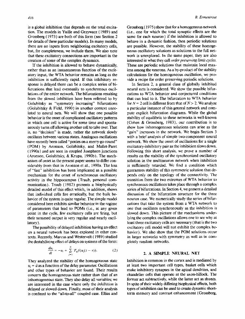
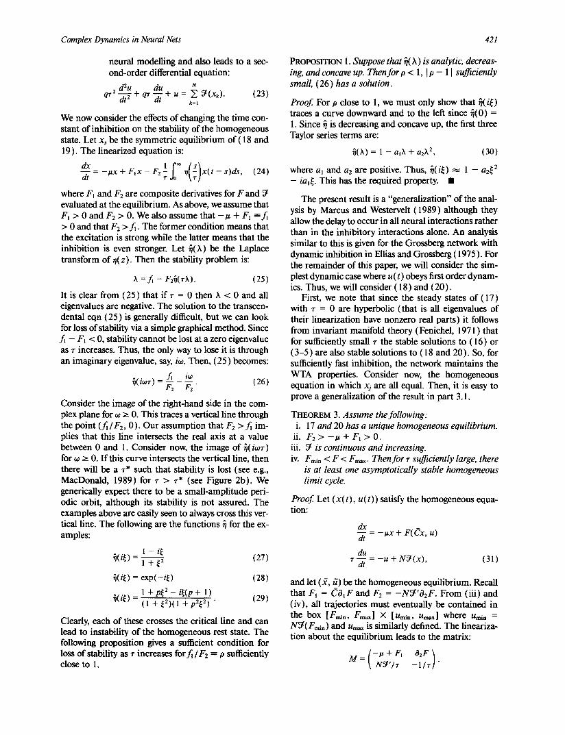
This theorem shows that for the N = 2 case, the bifurcation is a pitchfork and the resultant solutions are stable ifb > 0. The reason the case N = 2 is different is because of the reflection symmetry of the eigenvectors causes the quadratic terms in the bifurcation to disappear. For N > 2 there is an exchange of stability. The two cases are illustrated in Figure 1 for the Wilson- Cowan equations with instantaneous inhibition. The abscissa is the bifurcation parameter (ace) and the or- dinate is xl. In Figure la, the bifurcation is supercritical and there are two stable branches. These correspond to x~ "winning" and x2 "winning," respectively. Since N = 2, these equilibria are also stable solutions to (3- 5 ). Figure 1 b shows the case N > 2 (here, N = 8 ). The theorem is valid in the neighborhood of the exchange of stability, but the numerical solutions show a turning point in which the large amplitude upper branch appears. Only the upper branch and the left hand part of the symmetric branch are stable solutions to the full problem to the full system (3-5). For the lower supercritical branch to the right of the bifurcation point, the expressionf~2 from Theorem 2 is positive.

A generalization of (3-5) incorporates excitatory interactions; we replace (3) by:

N

dxj = -I~xj + F( ~ CjkXk, U; a). (16) dt k=~

If we make the ansatz that for each j , Z Cjk = C, then k

there is still a homogeneous solution to (16) and we can examine its stability. This assumption means that all excitatory cells receive the same total excitatory stimulation. If, in addition, Cjk = C ( j - k ) >-- O, the analysis is straightforward and is considered in the Ap- pendix. The case analyzed above concerned only Cjk = ~ j k .

We remark that Cohen and Grossberg (1983) prove that networks of the type described in this section have an explicit Liapunov function and so, with arguments that imply boundedness of trajectories, they show that all solutions tend to equilibria. For certain classes of problem, they are able to shed some light on the nature of these solutions. Our tack in this section is somewhat different in that we have attempted to analyze how this behavior can arise from a model which does not admit nontrivial patterns of activity. Furthermore, the results depend intimately on the existence of distributed excitation which is explicitly forbidden in their paper.

3. SYNCHRONOUS SOLUTIONS AND STABILITY

3.1. A Two Variable Example

Suppose that we have a single excitatory cell with recurrent inhibition. Unlike the previous section, we will

Lt9

I I I

L r } x

O

U /

1.0 2 . 0 3,0 4.0 5.0 8_ee

(a)

o I I I I I

S

I U

S

i I I I s I • 0 2 . 0 3 . 0 4 .0 5 . 0 6 . 0 7 . 0 8 . 0

a._ee

(b)

FIGURE 1. Bi furcat ion diagram for the Wilson-Cowen equations when N = 2 ( a ) and N = 8 ( b ) . x l is shown along the y-axis and or. along the x-axis. Parameters are , ~ = 8, aj, = 20, 0e = 1, and 0~ = 8. Turning point (1) and exchange of stabi l i ty ( 2 ) are shown in ( b ) .

assume that the inhibition is dynamic. The Wilson- Cowan equations provide a simple example of this type of model. The equations for this model are:

420 B. Ermentrout

dx - - = - x + f ( e l~x - O l i e U - - O e ) dt

du 1 -- ( - -U + f(OteiX -- Oi) ). (17)

dt r

The time-constant of the inhibition is given by r. We let f ( x ) = ( 1 + tanh x ) / 2 and choose parameters, O/ee ,

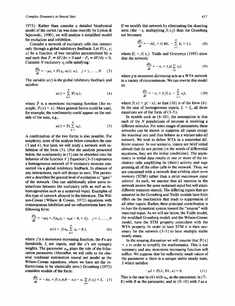
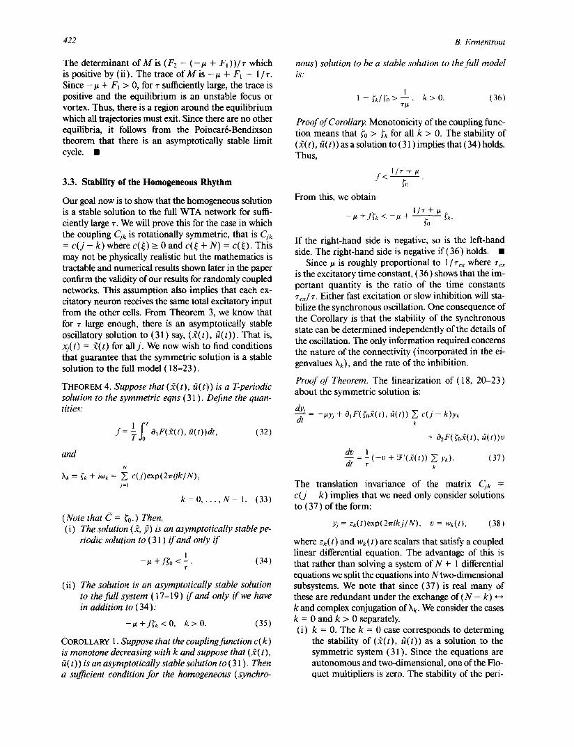
aei, aie, Oe, and 0i, so that there is a unique equilibrium point. For r small enough (i.e., fast inhibition), this rest state is stable. As the inhibition slows down, there is a Hopf bifurcation to periodic orbits. Further increases in r produce an oscillation that is more and more of the relaxation type. It is clear from (17) that all solutions must be bounded (indeed with f chosen above, if x(0) and u(0) are chosen from the interval (0, 1 ) they will remain there for all time.) The Poincar6- Bendixson theorem (Hirsch & Smale, 1974) then implies the existence of at least one stable periodic solution if the unique equilibrium is unstable. Figure 2a illus- trates the phase-plane for (17) and a typical oscillation. More details for ( 17 ) can be found in Ermentrout and Cowan (1979).

3.2. Stability Loss Due to Inhibitory Slowing

We now consider the stability of the homogeneous solution to (3-5) and (16) as the inhibitory timescale lengthens. We parametrize this timescale by a variable r and write:

dxj_ N dt gxj + F( ~ CjkXk, U(t); a), (18)

k=l

where u(t) satisfies the following functional equation:

U ( t ) = r rl ~ ~ ( X k ( t -- s ) ) d s , (19) k= l

and 71(z) is a nonnegative temporal kernel with integral 1. Thus,

N

lim u(t) --* ~ Y(Xk) , r ~ O k - I

and we recover (3-5, 16). Note that we could "move" the nonlinearity outside the summation in (19) to obtain the analogue of(4). We wish to explore the stability of the symmetric steady state as a function of the time- constant r of the inhibition. Before continuing with the analysis, we consider a few simple examples. Example 1. n(z) = exp( -z ) . Then (19) becomes the

familiar first order equation:

du N r --~ + u = Z ff:(Xk). (20)

k = l

Example 2. o(z) = 6(z - 1 ). Then (19) is the delayed excitation:

N

u(t) = ~, ~ 7 ( x k ( t - r ) ) . (21) k = l

U ' ~ 0

× ' = 0

Y

(a)

1

×

(b)

FIGURE 2a. Phase-plane of the two-cell Wilson-Cowan model showing nuIl-clines and limit cycle. Parameters are: a, . = 14, a,j = 15, aj, = 15, #. = 1, #l = 8, r = 1, (b) complex plane showing the intersection of the critical curves for eqn (26) .

Example 3. O(z) = z exp( -z ) . This kernel is the familiar "alpha" function used to model the impulse response in many neural models (see e.g., pages 177 and 327 in Koch & Segev, 1989 ). u (t) satisfies the second-order differential equation:

r 2 d 2 u r d u N - ~ + --~ + u = ~, ~(Xk) . (22)

k = !

Example 4. , (z ) = ( exp( -z ) - e x p ( - z / q ) ) / ( 1 - q) .

This kernel also appears frequently in


neural modelling and also leads to a second-order differential equation:

dEll du N qr 2 - ~ + qr -d~ + u = ~, Y(Xk). (23)

k=l

We now consider the effects of changing the time constant of inhibition on the stability of the homogeneous state. Let xs be the symmetric equilibrium of ( 18 and 19). The linearized equation is:

- - = -ILx + F t x - F2 - ~ x ( t - s)ds, (24) dt r

where F~ and F2 are composite derivatives for F and fit evaluated at the equilibrium. As above, we assume that F~ > 0 and F2 > 0. We also assume that - ~ + F~ ---f~ > 0 and that F2 > f~. The former condition means that the excitation is strong while the latter means that the inhibition is even stronger. Let ~(X) be the Laplace transform of ~(z). Then the stability problem is:

X =f~ - F2~I(rX). (25)

It is clear from (25) that if r = 0 then ~, < 0 and all eigenvalues are negative. The solution to the transcen- dental eqn (25) is generally difficult, but we can look for loss of stability via a simple graphical method. Since f~ - F~ < 0, stability cannot be lost at a zero eigenvalue as r increases. Thus, the only way to lose it is through an imaginary eigenvalue, say, i~o. Then, (25)becomes:

~( icor ) - ( 26 ) & &"

Consider the image of the right-hand side in the complex plane for ¢o >_ 0. This traces a vertical line through the point ( f l /F2 , 0). Our assumption that F2 >f~ implies that this line intersects the real axis at a value between 0 and 1. Consider now, the image of ~(i~or) for o~ >_ 0. If this curve intersects the vertical line, then there will be a r* such that stability is lost (see e.g., MacDonald, 1989) for r > r* (see Figure 2b). We generically expect there to be a small-amplitude periodic orbit, although its stability is not assured. The examples above are easily seen to always cross this vertical line. The following are the functions ~ for the examples:

1 - i ~ ~(i~)- 1 + ~2 (27)

~(i~) = exp(-i~) (28)

I + p ~ 2 - i ~ ( p + 1) ~(i~) = ( 1 + ~2)( 1 + p2~Z) • (29)

Clearly, each of these crosses the critical line and can lead to instability of the homogeneous rest state. The following proposition gives a sufficient condition for loss of stability as r increases forf~/F2 =- 0 sufficiently close to 1.

PROPOSITION 1. Suppose that ~( ~ ) is analytic, decreasing, and concave up. Then for o < l, I o - 11 sufficiently small, (26) has a solution.

Proo f For O close to 1, we must only show that ~(i~) traces a curve downward and to the left since ~(0) = 1. Since ~ is decreasing and concave up, the first three Taylor series terms are:

~(~k) = 1 - - a l Jk + a2k 2, (30)

where a~ and a2 are positive. Thus, ~(i~) ~ 1 - a2~ 2 - ia~ . This has the required property. •

The present result is a "generalization" of the analysis by Marcus and Westervelt (1989) although they allow the delay to occur in all neural interactions rather than in the inhibitory interactions alone. An analysis similar to this is given for the Grossberg network with dynamic inhibition in Ellias and Grossberg (1975). For the remainder of this paper, we will consider the sim- plest dynamic case where u (t) obeys first order dynamics. Thus, we will consider ( 18 ) and (20).

First, we note that since the steady states of (17) with r = 0 are hyperbolic (that is all eigenvalues of their linearization have nonzero real parts) it follows from invariant manifold theory (Fenichel, 1971 ) that for sufficiently small r the stable solutions to (16) or (3-5) are also stable solutions to ( 18 and 20). So, for sufficiently fast inhibition, the network maintains the WTA properties. Consider now, the homogeneous equation in which xj are all equal. Then, it is easy to prove a generalization of the result in part 3.1.

THEOREM 3. A s s u m e the following: i. 17 and 20 has a unique homogeneous equilibrium.

ii. F 2 > - ~ + F~ > 0. iii. fit is continuous and increasing. iv. F m i n < F < Fma~. Then fo r r sufficiently large, there

is at least one asymptotical ly stable homogeneous l imit cycle.

Proof Let (x (t), u (t) ) satisfy the homogeneous equation:

dr - - = - # . x + F ( C x , u) dt

du r--~ = - u + N ~ ( x ) , (31)

and let (~, ~7) be the homogeneous equilibrium. Recall that F~ = CO~F and F 2 = -Nf i t 'O2F. From (iii) and (iv), all trajectories must eventually be contained in the box [F=i., Fmax] X [Umi., U=~] where u~i, = Nfit(F=in) and Um~x is similarly defined. The linearization about the equilibrium leads to the matrix:

( - . + rl 02F I M = \ N T ' / r - l / r ] "

422 B. Ermentrout

The determinant of M is ( Fz - ( - # + Fl ) ) / r which is positive by (ii). The trace of M is - g + F I - 1 / r. Since -/~ + F~ > 0, for r sufficiently large, the trace is positive and the equilibrium is an unstable focus or vortex. Thus, there is a region around the equilibrium which all trajectories must exit. Since there are no other equilibria, it follows from the Poincar~-Bendixson theorem that there is an asymptotically stable limit cycle. •

3.3 . Stabi l i ty of the H o m o g e n e o u s R h y t h m

Our goal now is to show that the homogeneous solution is a stable solution to the full WTA network for sufficiently large r. We will prove this for the case in which the coupling Cjk is rotationally symmetric, that is Cjk = c ( j - k) where c(~) > 0 and c(~ + N) = c(~). This may not be physically realistic but the mathematics is tractable and numerical results shown later in the paper confirm the validity of our results for randomly coupled networks. This assumption also implies that each excitatory neuron receives the same total excitatory input from the other cells. From Theorem 3, we know that for r large enough, there is an asymptotically stable oscillatory solution to (31) say, (~(t) , fi(t)). That is, xy(t) = ~(t) for al l j . We now wish to find conditions that guarantee that the symmetric solution is a stable solution to the full model ( 1 8 - 2 3 ) .

THEOREM 4. Suppose that ( ~( t ), ~( t ) ) is a T-periodic solution to the symmetric eqns (31 ). Define the quan- tities:

and

lf0~ f = -~ OiF(.~(t), a(t))dt, (32)

N

Xk =-- fk + iwk = ~ c(j)exp(27rijk/N), j = l

k = 0 . . . . . N - 1. (33)

(Note that C = ~o. ) Then, ( i ) The solution ( ~, fi) is an asymptotically stable pe-

riodic solution to (31 ) i f and only i f

1 - i t +f~o < - . (34)

-g

(ii) The solution is an asymptotically stable solution to the full system (17-19) i f and only i f we have in addition to (34):

-U +f~'k < 0, k > 0 . (35)

COROLLARY 1. Suppose that the coupling function c( k ) is monotone decreasing with k and suppose that ( Y( t ), ft ( t) ) is an asymptotically stable solution to ( 31 ). Then a sufficient condition for the homogeneous (synchro-

From this, we obtain l / T + #

- # +f~'k < --U + - - ~'k- ~'0

nous) solution to be a stable solution to the full model is:

1 1 - ~k/~0 > - - k > 0. (36)

7"~t '

Proof of Corollary. Monotonicity of the coupling function means that ~'o > ~'k for all k > 0. The stability of (2( t ) , ri(t)) as a solution to (31 ) implies that (34) holds. Thus,

l i t + #

~o

If the right-hand side is negative, so is the left-hand side. The right-hand side is negative if (36) holds. •

Since u is roughly proportional to 1/rex where rex is the excitatory time constant, (36) shows that the important quantity is the ratio of the time constants rex/r. Either fast excitation or slow inhibition will sta- bilize the synchronous oscillation. One consequence of the Corollary is that the stability of the synchronous state can be determined independently of the details of the oscillation. The only information required concerns the nature of the connectivity (incorporated in the eigenvalues Xk), and the rate of the inhibition.

Proof of Theorem. The linearization of (18, 20-23) about the symmetric solution is:

- - - -#yj + O,F(~o2(t), O(t)) ~ c(j - k)yk dt k

+ OEF(~oY(t), ft(t))v

dv 1 - ( - v + ~t ' (2( t ) ) ~ Yk). (37)

dt r k

The translation invariance of the matrix Cjk =-- c ( j -- k) implies that we need only consider solutions to (37) of the form:

yj = zk( t)exp(2rikj /N), v = wk(t), (38)

where zk(t) and wk(t) are scalars that satisfy a coupled linear differential equation. The advantage of this is that rather than solving a system of N + 1 differential equations we split the equations into Ntwo-dimensional subsystems. We note that since (37) is real many of these are redundant under the exchange o f ( N - k) *--, k and complex conjugation of ~k. We consider the cases k = 0 and k > 0 separately. (i) k = 0. The k = 0 case corresponds to determing

the stability of (2(t) , ti(t)) as a solution to the symmetric system (31 ). Since the equations are autonomous and two-dimensional, one of the Flo- quet multipliers is zero. The stability of the peri-

C o m p l e x D y n a m i c s in N eura l Ne t s 423

odic orbit is obtained by looking at the trace of the linearized system which is:

1 - # - - + O ~ F ( ~ o g ( t ) , a(t))~'o.

7"

Stability is guaranteed as long as the mean over one cycle of this is negative thus implying (34).

(ii) k + 0. Then (Z k , Wk) satisfy:

dz~ _

dt - - - --#Zk + d ~ F ( ~ o $ ( t ) , a ( t ) )XkZk

+ 02F(~o-~( t ) , ~ ( t ) ) W k

(39) dwk_ 1

wk. dt

There is no dependence of Wk on Zk since N

e x p ( 2 7 r i k j / N ) = O, k ~ O. j=l

Thus, (39) is a scalar equation and stability is assured if the real part of the mean value of

- # + O~F(~o.~(t) , a ( t ) ) X k

is negative. This is equivalent to (35). •

R e m a r k . The inequality (36) is fine for connected networks, but in the case in which c ( j - k) = 0 unless j = k (the situation analyzed in Section 2) this estimate is too crude since ~'k = ~0 for all k. The required condition is that - # + f~'o < 0. This is stronger than the condition required for stability with respect to homogeneous perturbations (eqn (34)). This means it is possible for a WTA network to maintain its properties even for very slow inhibition.

R e m a r k . The mode by which the loss of stability of the homogeneous oscillation is clear from the proof of Theorem 4. If the network is symmetric, then it is possible to lose stability at a Floquet multiplier of 1 and at a nonzero wavenumber, k. The fact that this wave number is nonzero means that it is possible to have spatially modulated solutions bifurcating from the homogeneous oscillation. If certain technical conditions on the nonlinearities hold (these conditions are generic) then, solutions that have the form:

x j ( t ) = .~(t) + p ( t ) c o s ( 2 7 r k j x ) + • • •

where p(t) is periodic. This solution which is period- ically modulated in space has the "order preserving" properties originally sought by Ellias and Grossberg (1975). Because of the symmetry, any single cell in this network can have the maximum magnitude and will maintain it for the duration of the periodic solution. The cell that has the maximal output is chosen de- pending on the initial conditions. Thus, this oscillating network has many of the same properties as the stationary system described in Section 2.

R e m a r k . The onset of oscillations in the present network is quite different from that described by Cohen ( 1988, 1990). There, he shows that the oscillations arise through the spatial spread of cooperative activity in the network.

We have shown that for r sufficiently small there is a very asymmetric behavior in which one neuron is tonically firing and remaining cells are off. For r sufficiently large, all cells synchronously oscillate. In the next section, we address the question of how the transition between these two totally different behaviors could occur through a numerical example of the Wil- son-Cowan neural net.

4. THREE CELL SYSTEM

In this section, we attempt to understand the mechanism that underlies the transition from a WTA network to the synchronized oscillatory state. To do this, we assume a ring of three excitatory cells with a connection to one other cell. We will fix all parameters except for r in such a way as to guarantee that for r = 0, the 3- ring has the WTA property. Our approach is to use numerical methods and bifurcation theory to understand the onset of the "burst-like" solutions. The model we study is:

dxl = - x t + F(oteeXt + cx2 - otieu - 0~)

dt

dx2 = - x 2 + F(aeeX2 + CX3 - c~i~U - 0~)

dt

dx3 = - - X 3 q- F ( o l e e X 3 -]- CX! -- OtieU -- Oe)

dt

du 1 - - = - ( - u + F(c te i (x l + x2 + x3) - Oi)), (40) dt

where Otee = 14, aei = 15, ale = 15, c = 2, Oe = 1, Oi =

8. We will let r vary from a small value to a value that is O( 1 ). Equation (40) is a multiexcitatory generalization ofeqn. (3-5). Numerical simulations of the Yuille model show identical behavior so that we suspect that the following is a general property of slowed inhibitory WTA networks.

4.1. Emergence of the WTA System

Let us first set r = 0 and study the steady states of this symmetrically coupled system. Suppose that c is fixed and small (say two as above). When ace is sufficiently small, there is a unique steady state and this is stable and symmetric with respect to the three variables X l ,

x 2 , and x3. As Otee increases, a saddle node bifurcation occurs in which six new equilibria are born in analogy with the results in Section 2. Of these, three are stable and three are unstable. The six occur in stable-unstable

424 B. Ermentrout

pairs and are related to each other by rotation of the indices due to the symmetric coupling of the system. These appear to remain for all larger values of Otee. There are thus, seven distinct equilibria, three asymmetric stable fixed points, one unstable symmetric fixed point, and three unstable asymmetric fixed points. It is possible, as we saw in Section 2, that there may be many other equilibria, but these are not relevant for the present analysis. For general N, similar behavior occurs and there will be 2N + 1 fixed points, N of which are stable.

4.2. Behavior as r Increases

For r small, the network behaves as a WTA system and there are three steady states corresponding to one of the xi large and the other two close to zero (for reference, x~ = 0.5277, x2 ~ x3 ~ 0, and u = 0.4178). In addition are the three unstable saddle points (Xl = 0.2688, x2 = 0.000484, Xa = 0.02213, and u = 0.02176), the two others are obtained by permuting the first three variables). As r increases the stable steady states lose stability at a Hopf bifurcation at approximately r = 0.17. This supercritical bifurcation leads to small amplitude periodic oscillations about the stable states. Since there are three rest states and the system is symmetric, there are then three stable periodic solutions corresponding to rhythms in which one cell oscillates about a "high" state and the other two remain nearly zero. We note that at this point, the network behaves as an oscillatory WTA system and has "order preserving limit cycles" in the sense of Ellias and Grossberg ( 1975 ). This is yet another route to order preserving cycles and is different from that described in Section 3.2. At a slightly larger value of r, r ~ 0.22, the saddle points simultaneously lose stability via Hopf bifurcations that give rise to three unstable periodic oscillations. Finally, to set the stage, we examine the symmetric state as r increases. For r small the symmetric state is unstable with a two-dimensional unstable manifold and a two-dimensional stable manifold. As r increases, there is a Hopf bifurcation to a stable (with respect to symmetric perturbations) periodic orbit. This is unstable as a solution to the full problem. As in Section 4.1 there may be other periodic orbits, but these appear to be the only relevant ones. In general, there will be 2 N + 1 periodic orbits of which N are stable, N are unstable, and the symmetric orbit is unstable.

4.3. Ponies on a Merry-Go-Round

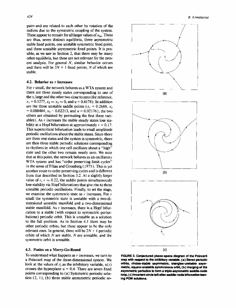
To understand what happens as r increases, we turn to a Poincar6 map of the three-dimensional system. We look at the values ofxj as the inhibitory variable, u( t ) crosses the hyperplane u = 0.4. There are seven fixed points corresponding to (a) Symmetric periodic solution (2, l ) , (b) three stable asymmetric periodic so-

/

(a)

(b)

(c)

FIGURE 3. Conjectured phase-space diagram of the Poincerb map with respect to the inhibitory variable. (a) Seven periodic orbits, circles-stable asymmetric, triangles-unstable asymmetric, square-unstable synchronous orbit, (b) merging of the asymmetric pedodice to form a triple asymmetric saddle-node loop, (c) invariant circle loft after seddle-node bifurcation leaving POM solutions.


0

x _ 2 ( t )

I1111 ' l l l l l ~ -- : ' ' ' ' , ' , I X--~ (t) ' ~ ,, ~ } i I

' ' ' n " " " " ' ' IIIllinli 11 I i I I I ' I I I

I I i I i I ~ II I I I I I I I I l i I % II I I I

I t I I ~ I I I I I I

i i II I I ~ I I I t I I I

; !1 i i 1| I%11 ' ' I ~ II fl I 11 , ' I 11 I I I I 1 | I ~l LI ~ I I I i I I I

' I I I ) 1 I I | l I i i | I I I I I I I I % I I i I |% I I I | | | I , , , , , , , , , |%, , , | , , , , 0 ,| ||

o

0 :19 38 57 76 95 :1].4 :133 :152 :17 t

(a)

II I I t I

190

I X 3

O

I t 3 " - i O

O

- 0 5

i I

I I 0.0 0.5 t•0 :1.5

x t+x 2+x 3 (b)

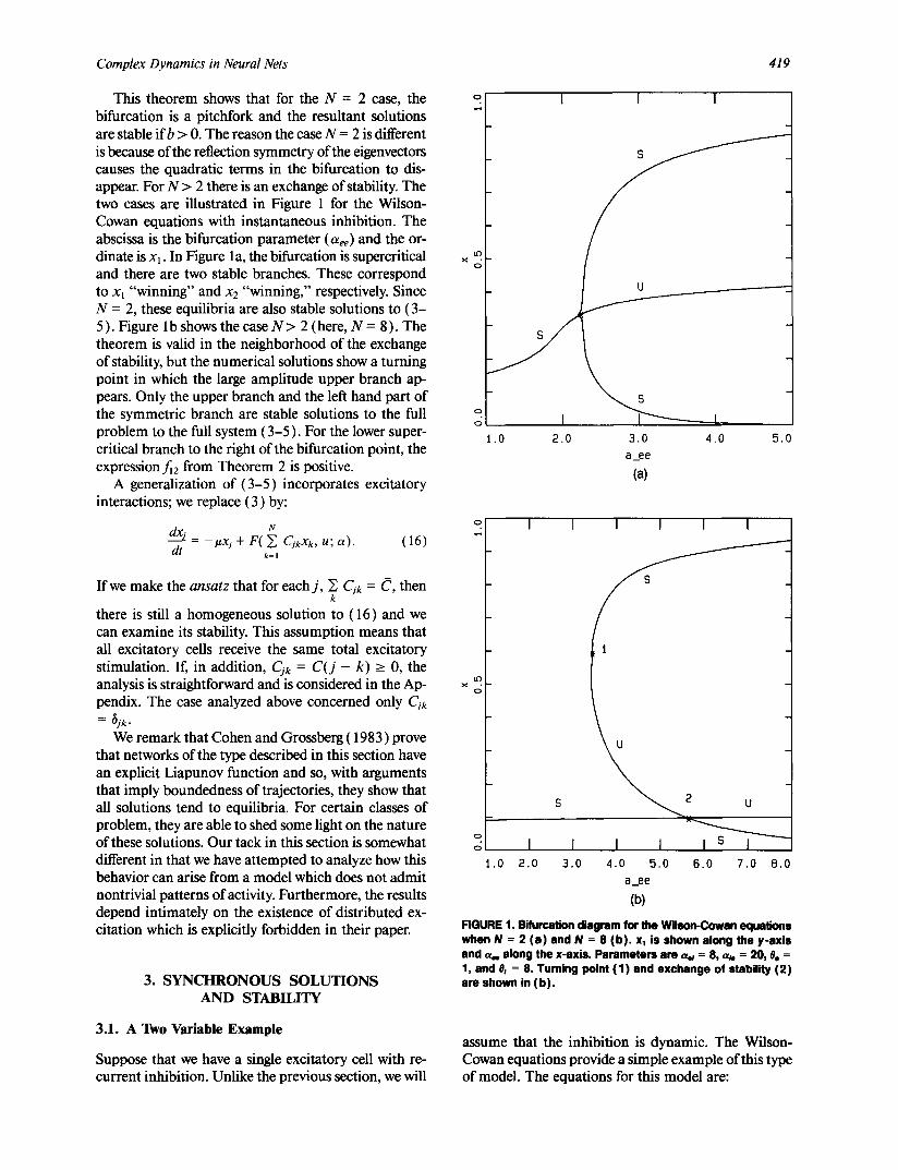
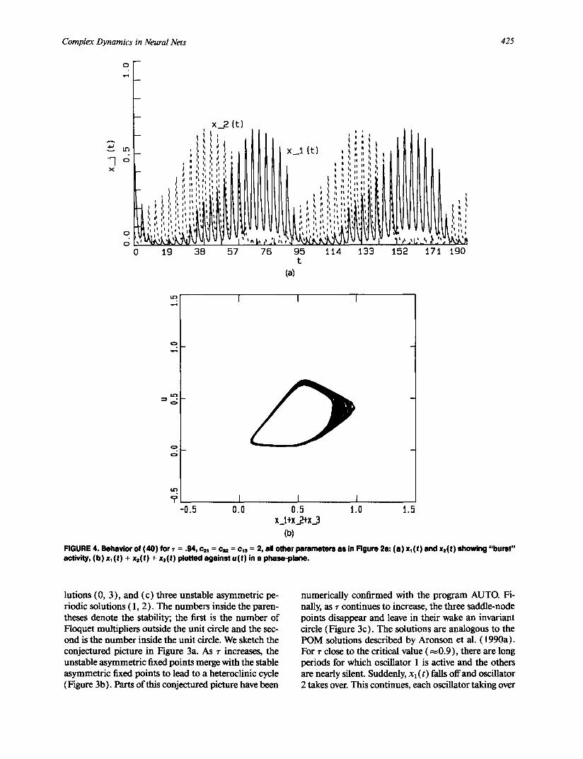
FIGURE 4. Behavior of (40 ) for r = .94, c21 = c . . = c,s = 2, all other parameters as in Figure 211: ( a ) x,(t) and x=(t) showing "burst" activity, (b ) x~(t) + xs(t) + x3(t) plotted against u(t) in a phase-plane.

lutions (0, 3 ), and (c) three unstable asymmetric periodic solutions ( 1, 2). The numbers inside the paren- theses denote the stability; the first is the number of Floquet multipliers outside the unit circle and the second is the number inside the unit circle. We sketch the conjectured picture in Figure 3a. As r increases, the unstable asymmetric fixed points merge with the stable asymmetric fixed points to lead to a heteroclinic cycle ( Figure 3b). Parts of this conjectured picture have been

numerically confirmed with the program AUTO. Fi- nally, as ~- continues to increase, the three saddle-node points disappear and leave in their wake an invariant circle (Figure 3c). The solutions are analogous to the POM solutions described by Aronson et al. (1990a). For r close to the critical value ( ~ 0 . 9 ) , there are long periods for which oscillator 1 is active and the others are nearly silent• Suddenly, Xl (t) falls off and oscillator 2 takes over. This continues, each oscillator taking over

426 B. Ermentrout

as its neighbor falls off. This is illustrated in Figure 4a. The lumped activities, ( x j ( t ) + x2 ( t) + x3 ( t ) ) almost lie on a dosed trajectory that is the same as a single excitatory-inhibitory pair as seen in Figure 4b.

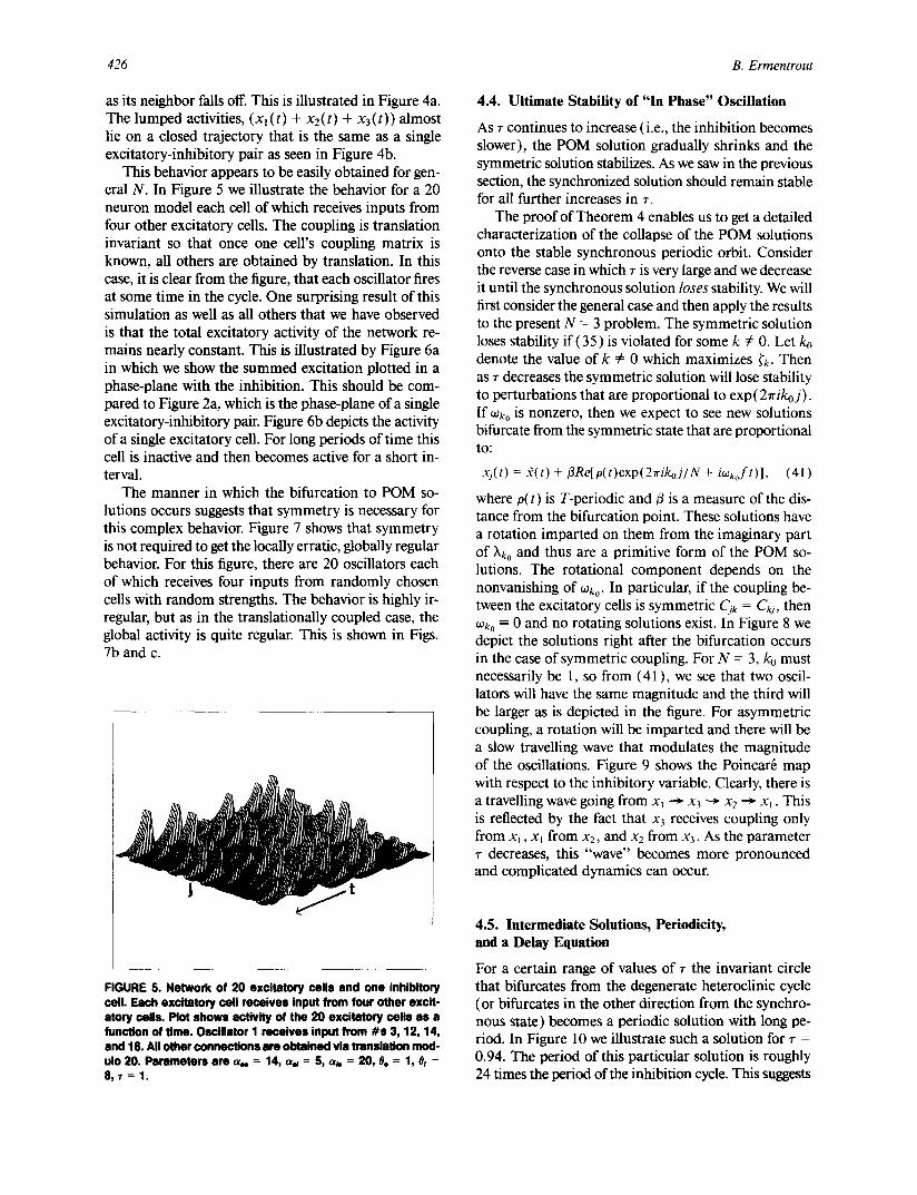
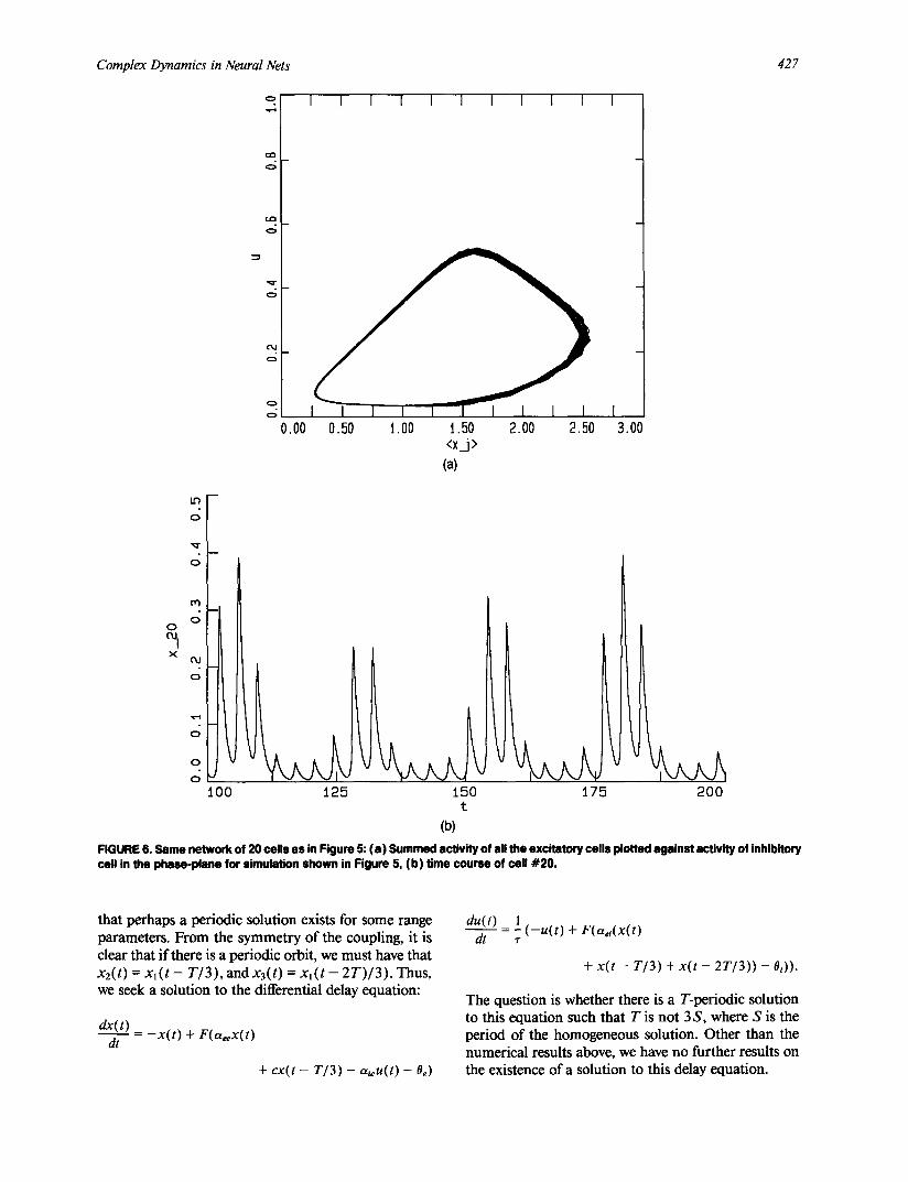
This behavior appears to be easily obtained for general N. In Figure 5 we illustrate the behavior for a 20 neuron model each cell of which receives inputs from four other excitatory cells. The coupling is translation invariant so that once one cell's coupling matrix is known, all others are obtained by translation. In this case, it is clear from the figure, that each oscillator fires at some time in the cycle. One surprising result of this simulation as well as all others that we have observed is that the total excitatory activity of the network remains nearly constant. This is illustrated by Figure 6a in which we show the summed excitation plotted in a phase-plane with the inhibition. This should be com- pared to Figure 2a, which is the phase-plane of a single excitatory-inhibitory pair. Figure 6b depicts the activity of a single excitatory cell. For long periods of time this cell is inactive and then becomes active for a short interval.

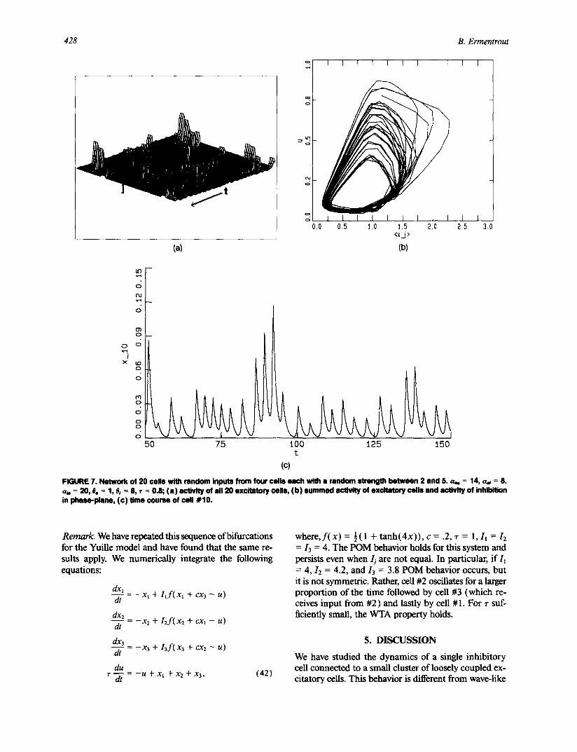
The manner in which the bifurcation to POM solutions occurs suggests that symmetry is necessary for this complex behavior. Figure 7 shows that symmetry is not required to get the locally erratic, globally regular behavior. For this figure, there are 20 oscillators each of which receives four inputs from randomly chosen cells with random strengths. The behavior is highly ir- regular, but as in the translationally coupled case, the global activity is quite regular. This is shown in Figs. 7b and c.

FIGURE 5. Network of 20 excitatory cells and one inhibitory ceil. Each excitatory ceil receives input from four other excit- story cells. Plot shows activity of the 20 excitatory ceils as a function of time. Oscillator I receives input from #s 3, 12, 14, and 16. All other connections are obtained via translation mod- ulo 20. Parameters are a, . = 14, o~ = 5, a,, = 20, 0. = 1, 0a = 8 , ~ = 1.

4.4. Ultimate Stability of "In Phase" Oscillation

As r continues to increase (i.e., the inhibition becomes slower), the POM solution gradually shrinks and the symmetric solution stabilizes. As we saw in the previous section, the synchronized solution should remain stable for all further increases in r.

The proof of Theorem 4 enables us to get a detailed characterization of the collapse of the POM solutions onto the stable synchronous periodic orbit. Consider the reverse case in which r is very large and we decrease it until the synchronous solution loses stability. We will first consider the general case and then apply the results to the present N -- 3 problem. The symmetric solution loses stability if (35) is violated for some k ~ 0. Let ko denote the value of k v t 0 which maximizes fk. Then as r decreases the symmetric solution will lose stability to perturbations that are proportional to exp (2~rikoj). If o~k0 is nonzero, then we expect to see new solutions bifurcate from the symmetric state that are proportional to:

xj(t) = £(t) + flRe[p(t)exp(2~rikoj/N + iO~koft)], (41)

where p(t) is T-periodic and fl is a measure of the dis- tance from the bifurcation point. These solutions have a rotation imparted on them from the imaginary part of kk0 and thus are a primitive form of the POM solutions. The rotational component depends on the nonvanishing of o~k0. In particular, if the coupling between the excitatory cells is symmetric C;k = Ckj, then ~k0 -= 0 and no rotating solutions exist. In Figure 8 we depict the solutions right after the bifurcation occurs in the case of symmetric coupling. For N = 3, k0 must necessarily be 1, so from (41 ), we see that two oscillators will have the same magnitude and the third will be larger as is depicted in the figure. For asymmetric coupling, a rotation will be imparted and there will be a slow travelling wave that modulates the magnitude of the oscillations. Figure 9 shows the Poincar6 map with respect to the inhibitory variable. Clearly, there is a travelling wave going from x~ --~ x3 --~ x2 --~ Xl. This is reflected by the fact that x3 receives coupling only from x~, x~ from x2, and x2 from x3. As the parameter r decreases, this "wave" becomes more pronounced and complicated dynamics can occur.

4.5. Intermediate Solutions, Periodicity, and a Delay Equation

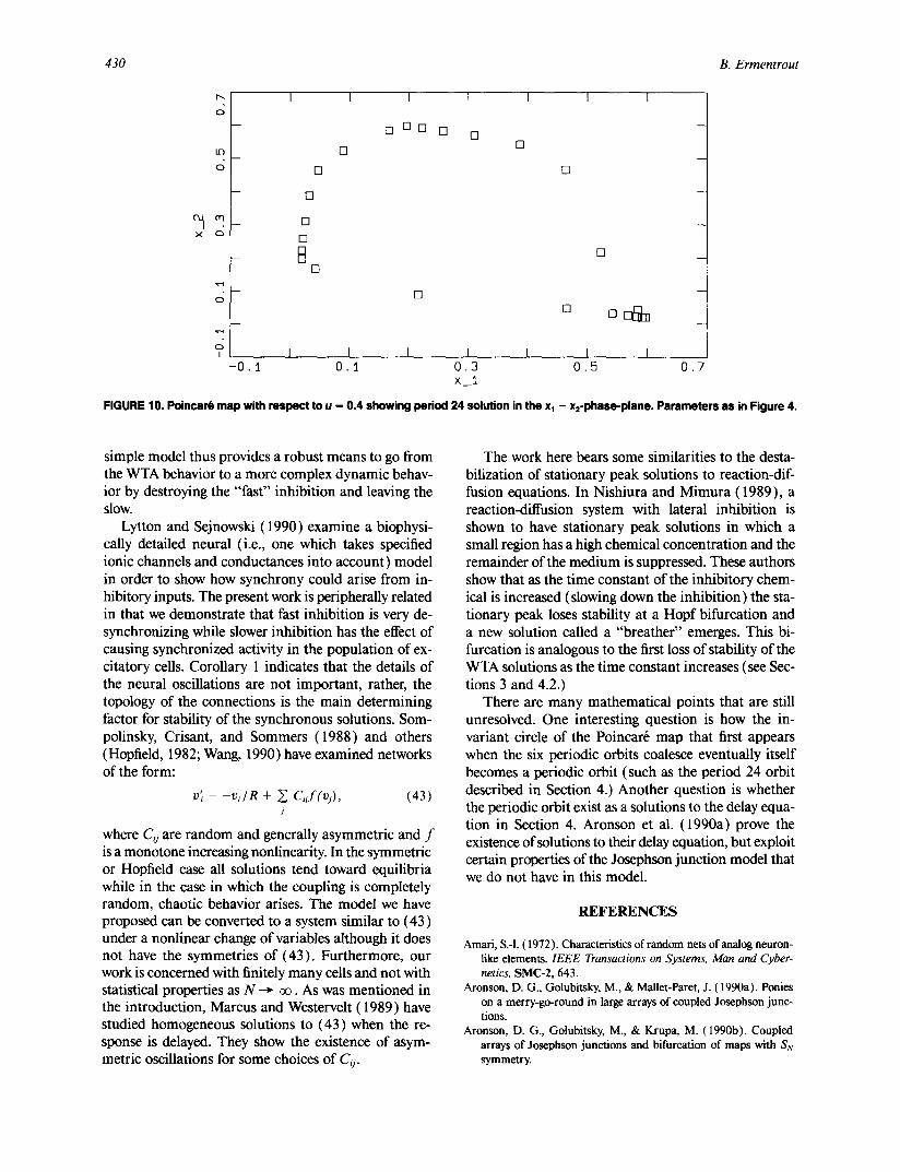
For a certain range of values of • the invariant circle that bifurcates from the degenerate heteroclinic cycle (or bifurcates in the other direction from the synchronous state) becomes a periodic solution with long period. In Figure 10 we illustrate such a solution for r = 0.94. The period of this particular solution is roughly 24 times the period of the inhibition cycle. This suggests


o

(:0

o

o

o

c~J

o

I I I I I I I I I I I

I I I I m I I I I I 0.00 0.50 t.00 ~.50 2.00 2.50

<X_]> (a)

1 3.00

o

x

o

• i

o

Od 0

o

o o

t 0 0 1 2 5 150 :17 ~, t

(b)

2OO

FIGURE 6. Same network of 20 ceils as in Figure 5: (a) Summed activity of all the excitatory ceils plotted against activity of inhibitory ceil in the phase-plane for simulation shown in Figure 5, (b) time course of cell #20.

that perhaps a periodic solution exists for some range parameters. From the symmetry of the coupling, it is clear that if there is a periodic orbit, we must have that x2(t) = x l ( t - T / 3 ) , and x3(t) = x ~ ( t - 2T)/3) . Thus, we seek a solution to the differential delay equation:

dx( t) dt = - x ( t ) + F ( a , , x ( t )

+ cx ( t - T / 3 ) - a ieu( t ) - Oe)

du( t) 1 ( - u ( t ) + F(aei (X( t )

dt r

+ x ( t - T / 3 ) + x ( t - 2T/3)) - 0i)).

The question is whether there is a T-periodic solution to this equation such that T is not 3S, where S is the period of the homogeneous solution. Other than the numerical results above, we have no further results on the existence of a solution to this delay equation.

428 B. E r m e n t r o u t

(a)

,,-;

c=,

o

I I I I I I I I [ l I

I I I I [ L [ [ I 0.0 0.5 1.0 1.5 2.0

< X ~ >

(b)

[

25 3.0

O

O

O3 O

O O

X tO O

O

iv] O

O

O O

O

f 50 75 iO0 125 150

t

(c)

FIGURE 7. Network of 20 cells with random inputs from four ceils each with • random strength between 2 and 5. a . . = 14, a., = 8, a,. = 20, e. = 1, 0a = 8, r = 0.8; (a ) activity of ell 20 excitatory cells, (b) summed activity of excitatory cells end activity of inhibition in phaea-piene, (c) time course of cell #10.

R e m a r k . We have repeated this sequence of bifurcations for the Yuille model and have found that the same results apply. We numerical ly integrate the following equations:

d x 1 - - = - -X l + I l f ( X t + CX3 -- U)

dt

d x 2 - - = --X2 + I 2 f ( x 2 + CXl -- U) dt

d x 3 - - = - x 3 + I 3 f ( x 3 + cx2 - u ) (it

du r - ~ = - u + xl + x2 + Xa, (42)

where, f ( x ) = ½(1 + t a n h ( 4 x ) ) , c = .2, r = l, I~ = 12 = 13 = 4. The P O M behavior holds for this system and persists even w h e n / j are not equal. In particular, i f 11 = 4, 12 = 4.2, and 13 = 3.8 P O M behavior occurs, bu t it is not symmetr ic . Rather, cell #2 oscillates for a larger propor t ion o f the t ime followed by cell #3 (which receives input f rom #2) and lastly by cell # 1. For r sufficiently small, the WTA proper ty holds.

5. D I S C U S S I O N

We have studied the dynamics of a single inhibi tory cell connected to a small cluster o f loosely coupled ex- ci tatory cells. This behavior is different f rom wave-like


,et

6

B

0 2 4 6 8 10 t

FIGURE 8. Solution to (40) for ~- s l ight ly smaller than the value for which the synchronous solution is stable. Asymmetric periodic solutions adse due to the symmetry of the coupling. Each ceil receives inputs from its neighbor of strength 2, • = 0.85, all other parameters as in Figure 2a.

and phase-locked oscillations observed in other systems of coupled neural oscillators (Ermentrout, 1982; Er- mentrout & Cowan, 1980). The numerical results presented show that one must be cautious in using neural inhibition as a means of enhancing contrast (i.e., as a means of selecting the maximal stimulus), for if the inhibition is allowed to behave dynamically, there can be difficulties when the inhibitory response is too slow.

Additionally, we have shown that synchronous oscillatory responses such as observed by Traub in his much more complete model for the hippocampus are also observed here. He has suggested that the loss of fast inhibition is the cause of the synchrony. We have

additional numerical support for this hypothesis. Sup- pose that we consider a population of excitatory neurons coupled to two different inhibitory cells, one fast and one slow. Our simulations indicate that the behavior of the fastest inhibitory cells determine the behavior of the coupled system. That is, if one inhibitor has a fast enough response to give the WTA property and the other has a slow response, it is the WTA property that emerges. This persists until the ratio of the influence of the "fast" cell to the "slow" cell is very small. Sim- ilarly, a cell that is slow enough to produce synchronous oscillations has little effect if the other inhibitory cell is capable of producing (e.g., POM solutions). Our

X O

-- x 3

O

LO

O

I I I J I I I I I I 0 ~. 0 2 0 3 0 4 0 5 0

t

FIGURE 9. Poincar0 map for (40 ) a tu - 0.4 with ~ = 1.2. Synchronous solution has lost stability to rotating "wave-l ike" perturbations. Coupling is asymmetric as in Figure 4. All other parameters as in Figure 3a.

430 B. Ermentrout

I I I I I I [ o

- D CID [] []

LQ [] D

0 [] []

-- []

× o []

[]

o [] --

[] r n ~ m

S , I I I I I [ I

-0.I 0.I 0.3 0 . 5 0.7 X_i

FIGURE 10. PoinearO map with respect to u -- 0.4 showing period 24 solution in the xl - x2-phase-plane. Parameters as in Figure 4.

simple model thus provides a robust means to go from the WTA behavior to a more complex dynamic behavior by destroying the "fast" inhibition and leaving the slow.

Lytton and Sejnowski (1990) examine a biophysically detailed neural (i.e., one which takes specified ionic channels and conductances into account) model in order to show how synchrony could arise from inhibitory inputs. The present work is peripherally related in that we demonstrate that fast inhibition is very de- synchronizing while slower inhibition has the effect of causing synchronized activity in the population of excitatory cells. Corollary 1 indicates that the details of the neural oscillations are not important, rather, the topology of the connections is the main determining factor for stability of the synchronous solutions. Som- polinsky, Crisant, and Sommers (1988) and others (Hopfield, 1982; Wang, 1990) have examined networks of the form:

v~ = - v , / g + ~ Cijf(vj) , (43) J

where C o are random and generally asymmetric and f is a monotone increasing nonlinearity. In the symmetric or Hopfield case all solutions tend toward equilibria while in the case in which the coupling is completely random, chaotic behavior arises. The model we have proposed can be converted to a system similar to (43) under a nonlinear change of variables although it does not have the symmetries of (43). Furthermore, our work is concerned with finitely many cells and not with statistical properties as N--~ ~ . As was mentioned in the introduction, Marcus and Westervelt (1989) have studied homogeneous solutions to (43) when the response is delayed. They show the existence of asymmetric oscillations for some choices of Cij.

The work here bears some similarities to the desta- bilization of stationary peak solutions to reaction-diffusion equations. In Nishiura and Mimura (1989), a reaction-diffusion system with lateral inhibition is shown to have stationary peak solutions in which a small region has a high chemical concentration and the remainder of the medium is suppressed. These authors show that as the time constant of the inhibitory chemical is increased (slowing down the inhibition) the stationary peak loses stability at a Hopf bifurcation and a new solution called a "breather" emerges. This bifurcation is analogous to the first loss of stability of the WTA solutions as the time constant increases (see Sec- tions 3 and 4.2.)

There are many mathematical points that are still unresolved. One interesting question is how the invariant circle of the Poincar6 map that first appears when the six periodic orbits coalesce eventually itself becomes a periodic orbit (such as the period 24 orbit described in Section 4.) Another question is whether the periodic orbit exist as a solutions to the delay equation in Section 4. Aronson et al. (1990a) prove the existence of solutions to their delay equation, but exploit certain properties of the Josephson junction model that we do not have in this model.

R E F E R E N C E S

Amari, S.-I. (1972). Characteristics of random nets of analog neuron- like elements. IEEE Transactions on Systems, Man and Cyber- netics, SMC-2, 643.

Aronson, D. G., Golubitsky, M., & Mallet-Parer, J. (1990a). Ponies on a merry-go-round in large arrays of coupled Josephson junctions.

Aronson, D. G., Golubitsky, M., & Krupa, M. (1990b). Coupled arrays of Josephson junctions and bifurcation of maps with SN symmetry.


Cohen, M. A. (1988). Sustained oscillations in a symmetric cooperative-competitive neural network: Disproof of a conjecture about content addressable memory. Neural Networks, 1, 217-22 I.

Cohen, M. A. (1990). The stability of sustained oscillations in symmetric cooperative-competitive networks. Neural Networks, 3, 609- 612.

Cohen, M. A., & Grossberg, S.(1983). Absolute stability of global pattern formation and parallel memory storage by competitive neural networks. IEEE Transactions on Systems, Man and Cy- bernetics, 13, 813-825.

Ellias, S. A., & Grossberg, S. (1975). Pattern formation, contrast control, and oscillations in the short-term memory of shunting on-center off-surround networks. Biological Cybernetics, 20, 69- 98.

Ermentrout, G. B. (1982). Asymptotic behavior of stationary, homogeneous neuronal nets. In Proceedings of the US-Japan Joint Seminar in Neural Nets. M. Arbib and S. Amari (Eds.), Springer Lecture Notes in Biomathematics, (Vol. 45, pp. 121-134). New York: Springer Verlag.

Ermentrout, G. B., & Cowan, J. D, (1979). Temporal oscillations in neuronal nets. Journal of Mathematical Biology, 7, 265-280.

Ermentrout, G. B., & Cowan, J. D. (1980). Secondary bifurcation in neuronal nets. SlAM Journal of Applied Mathematics 39, 323- 340.

Ermentrout, G. B., & Kopell, N. ( 1991 ). Multiple pulse interactions and averaging in systems of coupled neural oscillators. Journal of Mathematical Biology, 29, 195-217.

Fenichel, N. ( 1971 ). Persistence and smoothness of invariant mani- folds for flows. Indiana University Math Journal, 21, 193-226.

Golubitsky, M., & Field, M. (1990). Symmetry creation in nonlinear systems. SIAM Conference on Dynamical Systems, AS.

Gray, C. M., & Singer, W. (1989). Stimulus-specific neuronal oscillations in orientation columns of the cat visual cortex. PNAS, 86, 1698.

Grossberg, S. (1977). Pattern formation by the global limits of a nonlinear competitive interaction in n dimensions. Journal of Mathematical Biology, 4, 237-256.

Grossberg, S. (1973). Contour enhancement, short term memory, and constancies in reverberating neural networks. Studies in Ap- plied Math, Ll l , 213-257.

Hirsch, M. W., & Smale, S. (1974). Differential equations, dynamical systems, and linear algebra. Academic Press: New York.

Hopfield, J. (1982). Neural networks and physical systems with emergent collective computational abilities. PNAS, 79, 2554.

Kock, C., & Segev, I. (1989). Methods in neuronal modeling. MIT Press: Cambridge, MA.

Lytton, W., & Sejnowski, T. J. (1990). Inhibitory interneurons may help synchronize oscillations in cortical pyramidal neurons.

Macdonald, N. (1989). Biological delay systems: Linear stability theory Cambridge Studies in Mathematical Biology: 8, Cambridge University Press, New York.

Marcus, C. M., & Westervelt, R. M. (1989). Stability of analog neural networks with delay. Physics Review A, 39, 347-359.

Nishiura, Y., & Mimura, M. (1989). Layer oscillations in reaction- diffusion systems. SlAM Journal of Applied Mathematics, 49, 481 - 514.

Rumelhart, D., & Zipser, D. (1987). Feature discovery by competitive learning. In D. Rumelhart & J. McClelland (Eds.), Parallel Dis- tributed Processing (Vol. 1. pp. 151-193). MIT Press: Cambridge, MA.

Sompolinsky, H., Crisanti, A., & Sommers, H. ( 1988 ). Chaos in random neural networks. Physics Review Letters, 61, 259.

Traub, R. D. (1982). Simulation of intrinsic bursting in CA3 hip- pocampal neurons. Neuroscience, 7, 1233-1242.

Wang, X.-J. (1990). Spontaneous activity in a large neural net: between chaos and noise (preprin0.

Wilson, H. R., & Cowan, J. D. (1972). Excitatory and inhibitory interactions in localized populations of model neurons. Biophysical Journal, 12, 1-24.

Yuille, A. L., & Grzywacz, N. M. (1989). A winner-take-all mechanism based on presynaptic inhibition feedback. Neural Com- putation, 1, 334-347.

A P P E N D I X

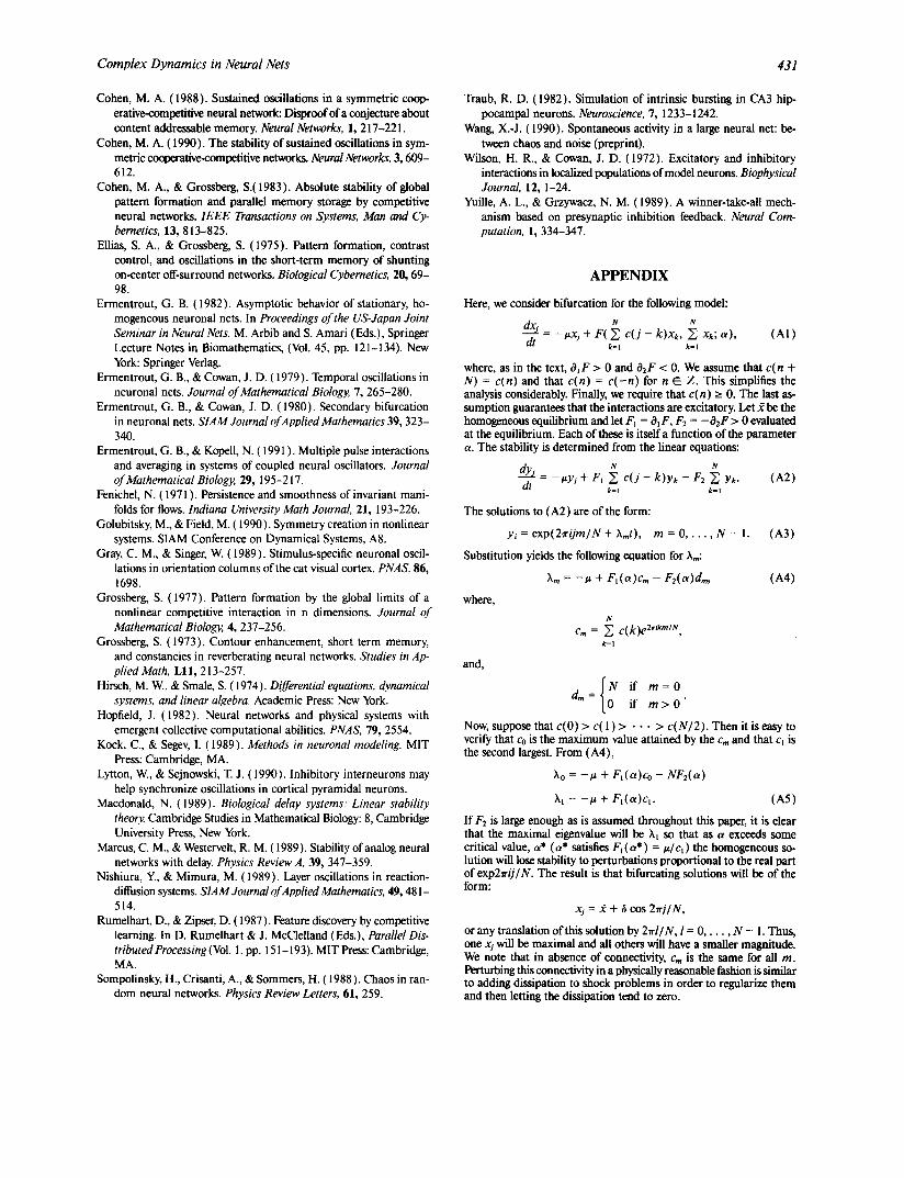
Here, we consider bifurcation for the following model: "

= - # x j + F ( ~ c( j - -k)Xk, ~, Xk;a), (AI) k=l k=l

where, as in the text, O~F > 0 and 02F < 0. We assume that c(n + N) = c(n) and that c(n) = c( -n) for n ~ Z. This simplifies the analysis considerably. Finally, we require that c(n) > O. The last assumption guarantees that the interactions are excitatory. Let .~ be the homogeneous equilibrium and let F~ = 01 F, F2 = -02F > 0 evaluated at the equilibrium. Each of these is itself a function of the parameter a. The stability is determined from the linear equations:

dyj _ -#YJ N - - - + Fl Z C(J - k)y k -/72 Z Yk. (A2) dt k=l k=l

The solutions to (A2) are of the form:

y~=exp(2*rijm/N+~mt), m = O . . . . . N - l . (A3)

Substitution yields the following equation for ~'m:

)~r,, = - # + Ft(a)c,,, - F2(a)dm, (A4)

where,

N

Cm = ~, c( k )e 2"~kmm, k=l

and,

if

if m > O "

Now, suppose that c(O) > c( 1 ) > • • • > c(N/2). Then it is easy to verify that Co is the maximum value attained by the c,. and that c~ is the second largest. From (A4),

•o = --# + Fl(a)Co - NF2(ot)

)~1 = --[,L + Fl(ot)ct. (A5)

If F2 is large enough as is assumed throughout this paper, it is clear that the maximal eigenvalue will be Xl so that as a exceeds some critical value, a* (a* satisfies Fl (a*) = #/c~ ) the homogeneous solution will lose stability to perturbations proportional to the real part of exp27rij/N. The result is that bifurcating solutions will be of the form:

= ~ + ~ cos 27rj/N,

or any translation of this solution by 2rl/N, l = 0 . . . . . N - 1. Thus, one xj will be maximal and all others will have a smaller magnitude. We note that in absence of connectivity, c,. is the same for all m. Perturbing this connectivity in a physically reasonable fashion is similar to adding dissipation to shock problems in order to regularize them and then letting the dissipation tend to zero.

Documents

Complex Dynamics in Winner-Take-All Neural Nets …bard/bardware/papers/wta-92.pdfComplex Dynamics in Winner-Take-All Neural Nets With Slow Inhibition BARD ERMENTROUT* University of