Embed Size (px)
Citation preview
1
Complex Behavior from a Simple Rule: Demonstration
with Lego Mindstorms NXT Kit
Honors Research Thesis
Presented in Partial Fulfillment of the Requirements for
the Degree Bachelor of Science with Honors Research Distinction
at The Ohio State University
By
Ruochen Yang
* * * * *
Department of Electrical and Computer Engineering
The Ohio State University
Spring 2013
Project Advisor:
Prof. Chris Baker
Dr. Graeme Smith

2
Acknowledgement
I would like to thank the following individuals for guidance, teamwork and support.
I appreciate Prof. Chris Baker and Dr. Graeme Smith’s continuous guidance over the past
year. Special thanks to Dr. Smith for your patience and dedicated mentorship. We have
been communicating roughly on a weekly basis to conduct tests and ways to analyze
data in order to understand and to solve problems encountered throughout the project.
I have learned a lot from you about how to be an effective researcher.
Thank you to the visiting scholar, Dr. Carmine Clemente. Even though your stay at the
Ohio State University was short, your finding on the ultrasonic sensor’s performance
was essential to my work and solved a problem that had bothered me for a month.
I respect and cherish the help from PhD students Saif Alsaif and Landon Garry for their
valuable and timely inputs when I needed some advice.
Thank you to Prof. Joel Johnson for introducing me to the ElectroScience Lab that led
me to Prof. Baker’s group and this project.
Last but not the least, I would not have been to the place I have now without my
parents, thanks to their support on my undergraduate study and my life abroad.
3
Abstract This report describes the successful implementation of two robots, built using Lego
Mindstorms, that demonstrate how complex animal behaviors can be replicated using a
simple algorithm to replicate a two neuron nervous system. The process of cognition
and decision making inside the mammalian brain occurs subtly but near instantaneously
and in a way that makes it hard to replicate synthetically. However, the understanding
of its behavior is valuable in multiple disciplines and it may be applied to future
technologies. In order to explore some behavior that relates to sensing and cognition,
the Lego Mindstorms NXT robot kit has been used. It is a sophisticated kit that includes
a programmable embedded computer, known as ‘the Brick’. This brick controls the
mechanical system made up from a set of modular Lego sensors and motors as well as
Lego parts. The base set of equipment and the customized add-ons provide an open-
ended platform that makes it possible to test a number of complex theories. The main
objective of the proposed project is to demonstrate how a complex behavior can be
simulated just based on some simple rule that represents the operation of neurons.
After investigating the capability and limitation of critical sensor used for the robot and
the motor specifications, the female cricket’s behavior of locating her mate in dark with
sound signals only, has been mechanically mimicked on Lego using two sound sensors
and two motors. Subsequently the echo location process of a bat using echoic flow
theory has been studied for collision avoidance. Preliminary results have had successful
and constant performance showing the potential of using Echoic Flow for steering
control on vehicles. This approach offers scientific researchers with an alternative to test
and experiment their hypothesis before applying it to large scale or real-life test
subjects, especially in cognitive sensing or intelligent control.

4
Contents Acknowledgement ........................................................................................................................... 2
Abstract ........................................................................................................................................... 3
Chapter 1. Introduction ............................................................................................................. 7
1.1 Background ...................................................................................................................... 7
1.2 The Cognitive Process and Decision Making ................................................................... 7
1.3 The Female Cricket Model and Prof. Barbara’s work ...................................................... 7
1.4 Echolocation in bats and the Echoic Flow theory............................................................ 8
1.5 Lego Mindstorms NXT robotics kit .................................................................................. 9
1.6 Overview of the thesis organization .............................................................................. 10
Chapter 2. Required Software and Hardware ......................................................................... 11
2.1 Software ........................................................................................................................ 11
2.2 Hardware ....................................................................................................................... 11
2.2.1 Lego Components Used ......................................................................................... 11
2.2.2 Other Hardware Components ............................................................................... 14
Chapter 3. Evaluation of Lego Sensors .................................................................................... 16
3.1 Background and Objectives ........................................................................................... 16
3.2 Sound sensor: Directivity ............................................................................................... 16
3.2.1 Setup ...................................................................................................................... 16
3.2.2 Results .......................................................................................................................... 17
3.3 Sound Sensor: Sampling Frequency .............................................................................. 18
3.3.1 Setup ............................................................................................................................. 18
3.3.2 Sampling time interval correction ......................................................................... 18
3.3.2 Results/Analysis ..................................................................................................... 19
3.4 Sound Sensor: Cable/Port Stability................................................................................ 21
3.4.1 Setup ...................................................................................................................... 21
3.4.2 Results/Analysis ..................................................................................................... 22
3.5 Sound Sensor: Range Sensitivity.................................................................................... 26
3.5.1 Setup ...................................................................................................................... 27
3.5.2 Results/Analysis ..................................................................................................... 27
3.6 Ultrasonic Sensor: Measurement Accuracy .................................................................. 28
3.6.1 Fixed Range, Various Angles .................................................................................. 28
5
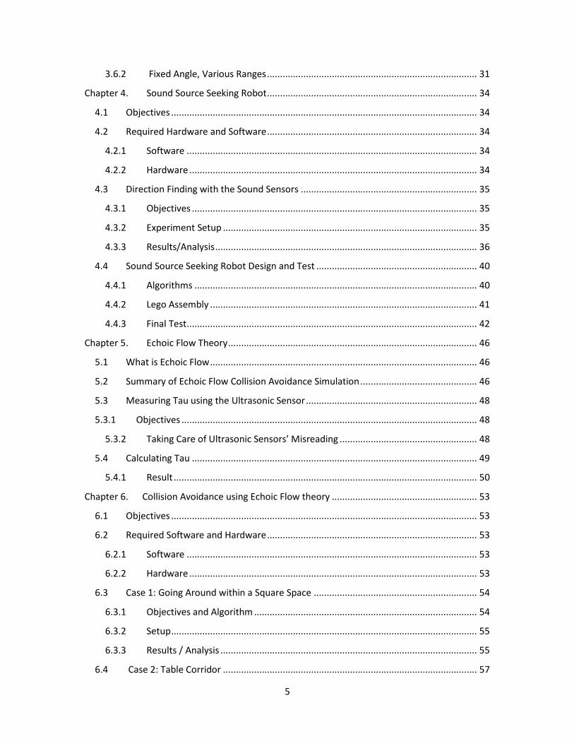
3.6.2 Fixed Angle, Various Ranges ................................................................................. 31
Chapter 4. Sound Source Seeking Robot ................................................................................. 34
4.1 Objectives ...................................................................................................................... 34
4.2 Required Hardware and Software ................................................................................. 34
4.2.1 Software ................................................................................................................ 34
4.2.2 Hardware ............................................................................................................... 34
4.3 Direction Finding with the Sound Sensors .................................................................... 35
4.3.1 Objectives .............................................................................................................. 35
4.3.2 Experiment Setup .................................................................................................. 35
4.3.3 Results/Analysis ..................................................................................................... 36
4.4 Sound Source Seeking Robot Design and Test .............................................................. 40
4.4.1 Algorithms ............................................................................................................. 40
4.4.2 Lego Assembly ....................................................................................................... 41
4.4.3 Final Test ................................................................................................................ 42
Chapter 5. Echoic Flow Theory ................................................................................................ 46
5.1 What is Echoic Flow ....................................................................................................... 46
5.2 Summary of Echoic Flow Collision Avoidance Simulation ............................................. 46
5.3 Measuring Tau using the Ultrasonic Sensor .................................................................. 48
5.3.1 Objectives .................................................................................................................. 48
5.3.2 Taking Care of Ultrasonic Sensors’ Misreading ..................................................... 48
5.4 Calculating Tau .............................................................................................................. 49
5.4.1 Result ..................................................................................................................... 50
Chapter 6. Collision Avoidance using Echoic Flow theory ........................................................ 53
6.1 Objectives ...................................................................................................................... 53
6.2 Required Software and Hardware ................................................................................. 53
6.2.1 Software ................................................................................................................ 53
6.2.2 Hardware ............................................................................................................... 53
6.3 Case 1: Going Around within a Square Space ............................................................... 54
6.3.1 Objectives and Algorithm ...................................................................................... 54
6.3.2 Setup ...................................................................................................................... 55
6.3.3 Results / Analysis ................................................................................................... 55
6.4 Case 2: Table Corridor .................................................................................................. 57
6
6.4.1 Objectives and Algorithm ...................................................................................... 57
6.4.2 Setup ...................................................................................................................... 57
6.4.3 Results / Analysis ................................................................................................... 58
6.5 Case 3: The Autonomous Collision Avoidance Robots .................................................. 60
6.5.1 Objectives and Algorithm ...................................................................................... 60
6.5.2 Setup ...................................................................................................................... 61
6.5.3 Results ................................................................................................................... 61
Chapter 7 Conclusion ................................................................................................................ 62
7.1 Conclusion ..................................................................................................................... 62
7.2 Wider Impact and Future Work..................................................................................... 62
7.3 Regulatory Rules and Industry Standards ..................................................................... 62
Appendix A .................................................................................................................................... 64
Appendix B..................................................................................................................................... 67
Appendix C ..................................................................................................................................... 68
Appendix D .................................................................................................................................... 71
References ..................................................................................................................................... 75
7
Chapter 1. Introduction
1.1 Background In this report two aspects pertaining to cognition are investigated. The first is a study of
the behavior of a simple neuronal interconnects that leads to quite subtle and
sophisticated behaviors as observed in the rituals of the female mating cricket. The
second is a new concept, based on an echoic form of flow fields, first used to explain
mammalian movement in complex scenarios. The objective is to implement sensing
systems that mimic these concepts and to investigate the resulting behaviors in a range
of contexts.
1.2 The Cognitive Process and Decision Making Almost all behavioral actions are the result of a process concerning cognition and
decision making inside the brain, which can be thought of as a biological supercomputer
that analyzes received information and reacts with nearly no delay. “Decision making is
a process that chooses a preferred option or a course of actions from among a set of
alternatives on the basis of given criteria or strategies.” [1] It implies that, in a slower
fashion, a computer should also be able to perform the cognitive process and output
reasonable reaction commands, as long as it has: some valid inputs, a set of rules, and
the corresponding choices.
1.3 The Female Cricket Model and Prof. Barbara’s work The behavior of a female mating cricket is very complicated. However, her brain, which
is physically very small, can process everything in less than a microsecond. She is able to
distinguish the mating chirps of males from other chirps, and once she has identified a
male ready to mate she can use the chirp to locate him. Her movement avoids open,
well-lit places where a predator could detect her [3]. When she is moving towards the
male cricket, if her left eardrum hears a signal louder than her right one, her right legs
will move faster than her left ones so that her body turns left; and vice versa for the
opposite side. It follows then that certain mechanisms of her complex behavior are
8
based on simple logic rules, and her cognition process for locating a sound source and
moving towards it is mechanically replicable.
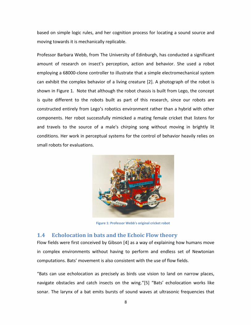
Professor Barbara Webb, from The University of Edinburgh, has conducted a significant
amount of research on insect’s perception, action and behavior. She used a robot
employing a 68000-clone controller to illustrate that a simple electromechanical system
can exhibit the complex behavior of a living creature [2]. A photograph of the robot is
shown in Figure 1. Note that although the robot chassis is built from Lego, the concept
is quite different to the robots built as part of this research, since our robots are
constructed entirely from Lego’s robotics environment rather than a hybrid with other
components. Her robot successfully mimicked a mating female cricket that listens for
and travels to the source of a male's chirping song without moving in brightly lit
conditions. Her work in perceptual systems for the control of behavior heavily relies on
small robots for evaluations.
Figure 1: Professor Webb's original cricket robot
1.4 Echolocation in bats and the Echoic Flow theory Flow fields were first conceived by Gibson [4] as a way of explaining how humans move
in complex environments without having to perform and endless set of Newtonian
computations. Bats’ movement is also consistent with the use of flow fields.
“Bats can use echolocation as precisely as birds use vision to land on narrow places,
navigate obstacles and catch insects on the wing.”[5] “Bats’ echolocation works like
sonar. The larynx of a bat emits bursts of sound waves at ultrasonic frequencies that

9
bounce off objects and return to the bat's ears, allowing the animal to identify what is in
the surrounding environment. The bat, in other words, navigates by the echoes that it
hears, differentiating among the different characteristics of those echoes.”[6]
Researchers from University of Maryland discovered that echolocating bats actually use
a nearly time-optimal strategy to intercept prey [7].
Inspired by the echolocating bats, many scientific researchers have been working on
steering control techniques for flight landing and other purposes. Dr Graeme Smith and
Prof. Christopher Baker, from The Ohio State University, developed the Echoic Flow
theory, a specific implementation of Lee’s flow fields [4], for cognitive radar sensing. The
most important parameter that the theory produces is Tau, which is the estimated time
before collision based on current situation detected by a radar system [8]. The Tau
relates to the current range, velocity and acceleration. Their simulation of a platform
equipped with a dual-beam monostatic radar system successfully navigated inside a
corridor for both a straight corridor and a square closed corridor case. This theoretically
proved that a system can navigate unhindered only relying on the Tau calculations. The
theory can potentially be applicable to some navigation aiding system for machines.
1.5 Lego Mindstorms NXT robotics kit
In this research, we used the robotics kit produced by Lego, known as Mindstorms NXT.
The kit includes a programmable embedded computer, known as ‘the Brick’ that
controls the system, a set of modular sensors and motors, and Lego parts to create the
mechanical systems. Besides the native language NXT-G, some general programming
languages can be used to program the brick such as, Java, C/C++, Python, and MATLAB.
Operation through these other languages is preferential for research work since it
permits their more powerful programming environments to be combined with ease of
robot construction available through the use of Mindstorms NXT. In addition, the base
set of equipment and the customized add-ons can cope with a few third-party sensors
and applications. These features of Lego Mindstorms robot provide researchers with a
10
very flexible open-ended platform to test a number of complex hypotheses. It has
advantages over many other test machines because it is straight forward to build and
program. The equipment does have certain limitations and methods to overcome them
will be explained in this report. Therefore, after suitable calibration, the Lego
Mindstorms NXT robot can play a meaningful role in scientific research.
1.6 Overview of the thesis organization The goal of this project is to show that a complex behavior can be simulated based on
very simple rules using the Lego Mindstorms NXT robot through two demonstrations.
Two Lego robots will be built to follow the process of cognition and decision making
inside an insect or animal nervous system. One robot will be designed to behave like a
female cricket and find its way towards a sound source while avoiding possible obstacles
without any external aid or instruction; the other one will be able to navigate
autonomously without colliding into anything in an area using the Tau parameter, time
before collision, calculated according to the Echoic Flow theory.
The report will cover experiments and analysis on the capabilities of critical Lego parts,
the design of the Lego robot and the final robot tests.
Chapter 2 will introduce the software and hardware used for this project, and
their basic functions.
Chapter 3 will focus on investigations of the Lego sound sensors and ultrasonic
sensors since they are the critical components for the two robot models.
Chapter 4 will explain how the sound source seeking robot is designed and its
results.
Chapter 5 will briefly talk about the Echoic Flow and summarize Dr Smith’s
simulation.
Chapter 6 will explain how the collision avoidance robot is designed and its
results.
Chapter 7 will conclude this report and state future work.

11
Chapter 2. Required Software and Hardware This chapter will be introducing all the software and hardware used for the project. The
function and brief performance of each Lego robot module will be discussed.
Performance of critical Lego parts will be further evaluated and explained in detail in
Chapter 3.
2.1 Software The following software components were used during the development of the robot:
a. MATLAB R2011b;
b. The RWTH Mindstorms NXT MATLAB Toolbox, developed by members of
the RWTH Aachen University for educational purpose, is a free open source
product and is subject to the GNU GENERAL PUBLIC LICENSE [9];
c. The Phantom Lego NXT Driver, which allows the computer to communicate
with the Lego robot via an umbilical USB cable.
The Lego Mindstorms kit is provided with NXT-G, a graphical programming environment
developed by NI LabView. However, the variety of interactions between the PC and the
robot are limited under NXT-G making the product less suitable for scientific research.
MATLAB is a popular programming language with a toolbox available that allows
connection to the Lego control brick and sensors. It allows the user great control over
the Lego modules (sensors and motors), and a good way to store and analyze data.
Therefore, all programs will be written in MATLAB, version 2011b, for this project and
will be attached in the appendix section.
2.2 Hardware The following components from the Lego Mindstorms kit were used in the current
research.
2.2.1 Lego Components Used
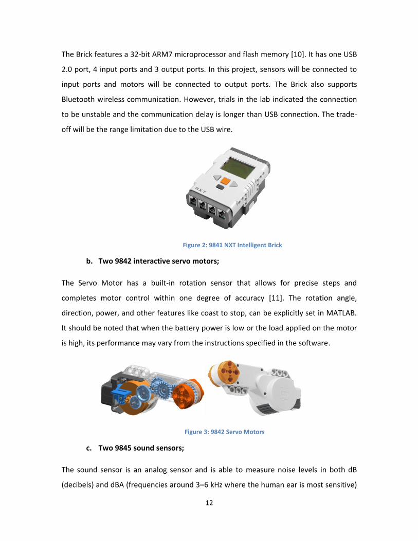
a. One LEGO Mindstorms 9841 NXT Intelligent Brick with six AA batteries;
12
The Brick features a 32-bit ARM7 microprocessor and flash memory [10]. It has one USB
2.0 port, 4 input ports and 3 output ports. In this project, sensors will be connected to
input ports and motors will be connected to output ports. The Brick also supports
Bluetooth wireless communication. However, trials in the lab indicated the connection
to be unstable and the communication delay is longer than USB connection. The trade-
off will be the range limitation due to the USB wire.
Figure 2: 9841 NXT Intelligent Brick
b. Two 9842 interactive servo motors;
The Servo Motor has a built-in rotation sensor that allows for precise steps and
completes motor control within one degree of accuracy [11]. The rotation angle,
direction, power, and other features like coast to stop, can be explicitly set in MATLAB.
It should be noted that when the battery power is low or the load applied on the motor
is high, its performance may vary from the instructions specified in the software.
Figure 3: 9842 Servo Motors
c. Two 9845 sound sensors;
The sound sensor is an analog sensor and is able to measure noise levels in both dB
(decibels) and dBA (frequencies around 3–6 kHz where the human ear is most sensitive)
13
[12]. Another output mode is accessible in MATLAB2011b, the raw 10-bit ADC mode (0 –
1023, silent to loud) based on measurements proportional to acquired voltage. Analog
to digital converter (ADC) gives an output based on a measured voltage.
, so Power is proportional to the ADC value squared. Only raw
ADC measurement mode will be used throughout this project.
Figure 4: 9845 Sound Sensor
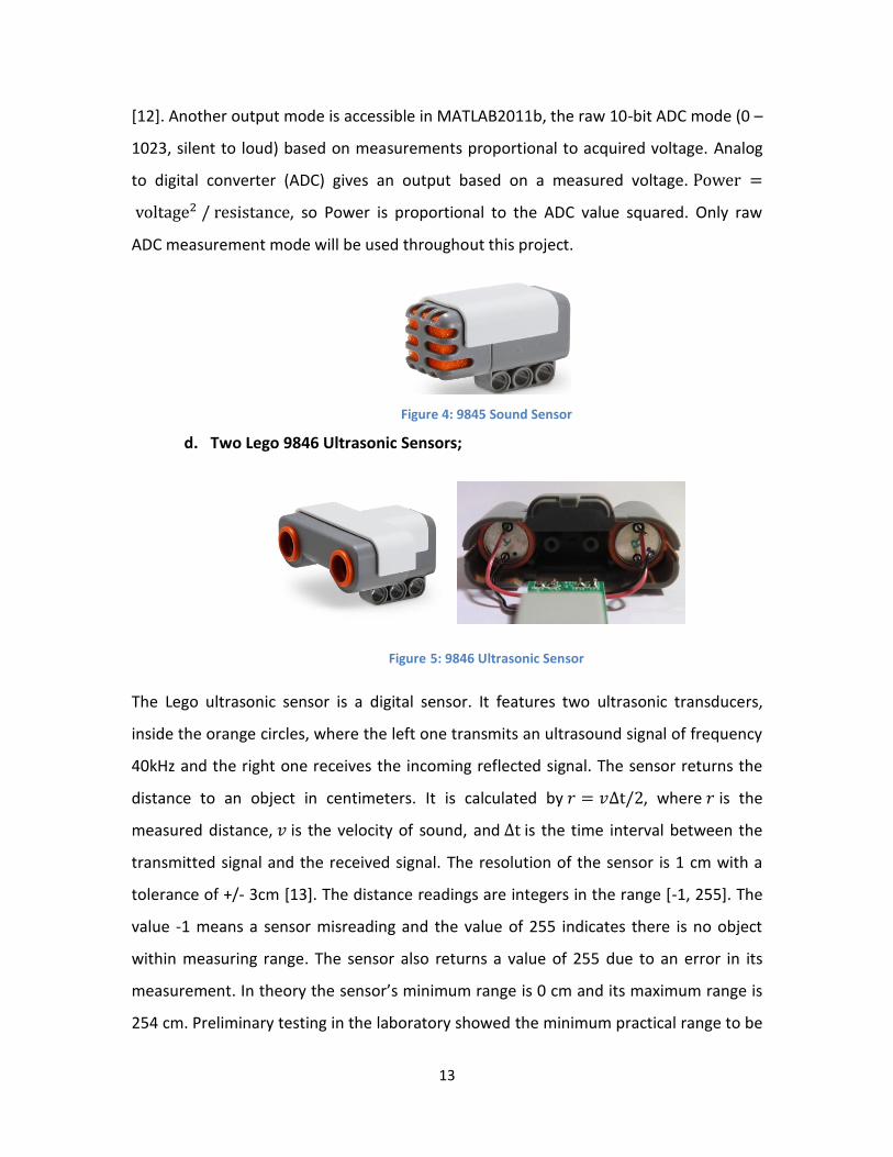
d. Two Lego 9846 Ultrasonic Sensors;
Figure 5: 9846 Ultrasonic Sensor
The Lego ultrasonic sensor is a digital sensor. It features two ultrasonic transducers,
inside the orange circles, where the left one transmits an ultrasound signal of frequency
40kHz and the right one receives the incoming reflected signal. The sensor returns the
distance to an object in centimeters. It is calculated by , where is the
measured distance, is the velocity of sound, and is the time interval between the
transmitted signal and the received signal. The resolution of the sensor is 1 cm with a
tolerance of +/- 3cm [13]. The distance readings are integers in the range [-1, 255]. The
value -1 means a sensor misreading and the value of 255 indicates there is no object
within measuring range. The sensor also returns a value of 255 due to an error in its
measurement. In theory the sensor’s minimum range is 0 cm and its maximum range is
254 cm. Preliminary testing in the laboratory showed the minimum practical range to be

14
5 cm. The maximum range depends on the surface of the object to be detected, large
and hard objects can be detected over a longer range than small and soft objects [14]. In
addition, the 1cm-resolution does not provide the full description of the sensor’s
accuracy. Objects with a surface perpendicular to the direction of the transmitted signal
can be detected more accurately than angled objects. This will be explained in detail in
Chapter 3. Echoes due to multipath can limit the practical range even further.
“An ultrasound pulse does not travel in a narrow straight line as a laser beam does.
Instead it spreads out like the light beam of a flashlight. As a result the sensor not only
detects objects directly in front of it, but also objects that are somewhat to the sides. As
a rule of thumb one can assume that objects that are within an angle 15 degrees to the
left or right are detected. The total angular width of the detection area is about 30
degrees. When using the sensor for obstacle avoidance this wide beam is an advantage.
When the sensor is used for mapping it is a drawback since objects appear to be wider
than they really are.” [14]
e. Four connection wires between motors/sensors and the brick;
f. One USB cable for PC/brick communication;
2.2.2 Other Hardware Components
In addition to the Lego Mindstorms kit, the following equipment was also utilized:
a. One RadioShack Mini Audio Amplifier and a 9V battery;
This speaker is not a highly refined apparatus. On its left side, it has an input port, an
output port, and a port for optional 9V DC adapter. On its right, a turning wheel can be
rotated to turn the speaker on/off and adjust the volume. There is no way to quantify
the output volume. Hence, it is hard to get back to the exact same volume after the
speaker has been turned off. Keeping the speaker on and untouched is assumed to
produce an unchanged volume. In addition, its output frequency range is 100 – 10 kHz
according to its user’s guide.

15
Figure 5: RadioShack Mini Audio Amplifier
b. A laptop running MATLAB2011b.
16
Chapter 3. Evaluation of Lego Sensors
3.1 Background and Objectives The sensors provided with the Lego robot are quite limited in their performance and this
will impact any experimentation performed. Unfortunately, Lego does not provide
sensor specifications detailed enough for scientific research. For our project, the Lego
sound sensor and ultrasonic sensor are the critical and the only ones used in the female
cricket and the collision avoidance robot models, respectively. It is therefore necessary
to understand the performance of the sensors so that deficiencies can either be
removed by calibration or are appropriately taken into account when the results are
interpreted.
3.2 Sound sensor: Directivity
3.2.1 Setup
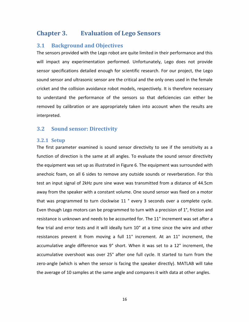
The first parameter examined is sound sensor directivity to see if the sensitivity as a
function of direction is the same at all angles. To evaluate the sound sensor directivity
the equipment was set up as illustrated in Figure 6. The equipment was surrounded with
anechoic foam, on all 6 sides to remove any outside sounds or reverberation. For this
test an input signal of 2kHz pure sine wave was transmitted from a distance of 44.5cm
away from the speaker with a constant volume. One sound sensor was fixed on a motor
that was programmed to turn clockwise 11 ° every 3 seconds over a complete cycle.
Even though Lego motors can be programmed to turn with a precision of 1°, friction and
resistance is unknown and needs to be accounted for. The 11° increment was set after a
few trial and error tests and it will ideally turn 10° at a time since the wire and other
resistances prevent it from moving a full 11° increment. At an 11° increment, the
accumulative angle difference was 9° short. When it was set to a 12° increment, the
accumulative overshoot was over 25° after one full cycle. It started to turn from the
zero-angle (which is when the sensor is facing the speaker directly). MATLAB will take
the average of 10 samples at the same angle and compares it with data at other angles.

17
Figure 6: Sensor Directivity Test Setup
3.2.2 Results
The results of the testing for the two sound sensors are presented in Figures 7 and 8.
They are polar plots indicating the received sound power at a given sensor angle for the
fixed range of 44.5cm. It is apparent that both sound sensors are nearly
omnidirectional, measuring the same power at all angles. For convenience, in the
directivity test section, all data were converted into decibel of sound power.
Figure 7: Directivity-Sensor 1 Figure 8: Directivity-Sensor
20
40
60
30
210
60
240
90
270
120
300
150
330
180 0
Sensor1 Directivity
20
40
60
30
210
60
240
90
270
120
300
150
330
180 0
Sensor2 Directivity
Anechoic Foam

18
3.3 Sound Sensor: Sampling Frequency
3.3.1 Setup
Lego does not provide information about the sampling capabilities of the sound sensors.
It is necessary to find out the estimated experimental value of the sampling frequency
of the sound sensors in order for them to work in the frequency range where they have
the best accuracy in measuring the power of a sound signal. If possible, it is also
desirable to learn whether the sound sensors are able to distinguish between different
sound signals (e.g. chirps, non-chirps).
Experiments in this section took place in a closed space formed by the anechoic foam
where only the Lego brick, housing the two sound sensors and the speaker were
located. Both devices were connected to a laptop that controls the speaker and sound
sensors through MATLAB. The speaker was 3cm away facing the sensor. The sensor was
timed to take 1000 samples for each sound signal frequency. The frequencies are: 50Hz,
75Hz, 100Hz, 125Hz, and 150Hz. The received data will be analyzed and compared for
each case, in both the time and the frequency domain.
3.3.2 Sampling time interval correction
To analyze data in the frequency domain, Fourier Transform has to be applied in
MATLAB which requires equal time intervals. During the data processing stage, a sample
time correction will take place in order to perform Fast Fourier Transform in MATLAB.
While a sample is stored, the corresponding time is also recorded. Due to uncontrollable
delays in both the Lego processor and the different loops that it runs through in
MATLAB, the time interval between two samples is not constant. It is necessary to
correct the intervals so that they equal each other and fit the requirement to Fourier
Transform the data sets. The total time that 1000 samples took will stay the same and
the interval will be assigned as the total time divided by 999 using the MATLAB function
linspace(a,b,n)where a is the start time, b is the end time and n=1000. Each data
sample will be interpolated to be corresponding to a new equally spaced time point
instead of the original recorded one. Samples with the corrected time will then be used

19
for Fourier Transform that will display properties of received data in the frequency
domain.
3.3.2 Results/Analysis
Figure 9 to 12 display results taken when the signal generated was a 50Hz pure sine
wave. The raw ADC data collected by the sensors will have their average value
subtracted so they will center at y = 0, which makes it easier to observe the main
frequencies of the waveform. For figures plotted in the frequency domain, an obvious
spike at a certain frequency indicates that the waveform formed by the sampled data
contains that certain frequency component.
Sensor 1 took 1000 samples in 3.0825s. After correcting the time intervals, the sampling
frequency was approximately 334.7673Hz. The raw data plot shown in Figure 10 clearly
shows that the waveform is composed by some very low frequency and some much
higher frequencies. The first two major peaks in the time domain signal occur at around
0.4s and 1.4s and the second and third peaks occur at around 1.4s and 2.8s; they
indicate frequency components of 1Hz and 1.4Hz. After a close up look at the raw data,
most of the small peaks are around 0.01s apart, which indicates a frequency component
of 100Hz. The Fast Fourier Transform of received data is shown in Figure 9. Obvious
spikes are at 100Hz and some unknown very low frequency less than 10Hz. The two
plots agree with each other.
Figure 9: 50Hz signal, Sensor1 Raw data Figure 10: 50Hz signal, Sensor1 FFT
0 0.5 1 1.5 2 2.5 3 3.5-60
-40
-20
0
20
40
60
80Raw Data
time
Raw
Data
- A
vera
ge
0 50 100 150 200 250 300 3500
1000
2000
3000
4000
5000
6000Fourier Transform
Frequency(Hz)
20
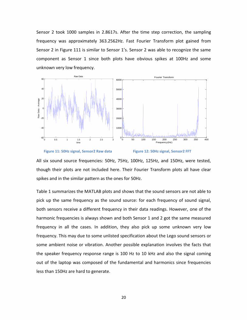
Sensor 2 took 1000 samples in 2.8617s. After the time step correction, the sampling
frequency was approximately 363.2562Hz. Fast Fourier Transform plot gained from
Sensor 2 in Figure 111 is similar to Sensor 1’s. Sensor 2 was able to recognize the same
component as Sensor 1 since both plots have obvious spikes at 100Hz and some
unknown very low frequency.
Figure 11: 50Hz signal, Sensor2 Raw data Figure 12: 50Hz signal, Sensor2 FFT
All six sound source frequencies: 50Hz, 75Hz, 100Hz, 125Hz, and 150Hz, were tested,
though their plots are not included here. Their Fourier Transform plots all have clear
spikes and in the similar pattern as the ones for 50Hz.
Table 1 summarizes the MATLAB plots and shows that the sound sensors are not able to
pick up the same frequency as the sound source: for each frequency of sound signal,
both sensors receive a different frequency in their data readings. However, one of the
harmonic frequencies is always shown and both Sensor 1 and 2 got the same measured
frequency in all the cases. In addition, they also pick up some unknown very low
frequency. This may due to some unlisted specification about the Lego sound sensors or
some ambient noise or vibration. Another possible explanation involves the facts that
the speaker frequency response range is 100 Hz to 10 kHz and also the signal coming
out of the laptop was composed of the fundamental and harmonics since frequencies
less than 150Hz are hard to generate.
0 0.5 1 1.5 2 2.5 3-60
-40
-20
0
20
40
60Raw Data
time
Raw
Data
- A
vera
ge
0 50 100 150 200 250 300 350 4000
1000
2000
3000
4000
5000
6000Fourier Transform
Frequency(Hz)

21
Signal Frequency 50Hz 75Hz 100Hz 125Hz 150Hz
Frequency Measured by Sensor 1 100Hz 150Hz 150Hz 100Hz 50Hz
Frequency Measured by Sensor 2 100Hz 150Hz 150Hz 100Hz 50Hz
Table 1: Comparison Table of Actual and Sampled Frequencies
Even though the power should vary for different signal frequencies, the data will appear
identical for both the fundamental frequency and any that are aliased. Working through
MATLAB, the sampling frequency of the sound sensors varies because of external and
some unconsidered delays. Since the lowest frequency is 307samples/sec, it is
reasonable to assume that the sensors are able to pick up frequencies under 150Hz
without aliasing.
The knowledge gained in this section also implies that the Lego sound sensors cannot
practically record a piece of sound unless it is lower than 150Hz. However, sound signals
below 150Hz are hard to generate with the available equipment. Therefore, recognizing
chirps will not be studied in this project; we will be using the raw ADC data for the
design and will not use the frequency detected by sound sensors.
3.4 Sound Sensor: Cable/Port Stability The Lego Mindstorms NXT brick has four input ports and three output ports. Since Lego
sound sensors are analog sensors, Hardware configurations and the local environment
may therefore influence measured data. The following tests will determine the effects
of Sensor/Cable/Port variation on the collected ADC mode raw data. They also allow a
decision to be made about the combination for the best performance and that will be
kept until the end of the project.
3.4.1 Setup
The difference in data received by MATLAB due to various cable, sensor and port
combinations is studied so that it may be properly compensated for the development of
the final cricket robot. The configurations are determined as there are only two choices
for sensor, cable or port. Six combinations, summarized, in Table 2 were tested and
compared:
22
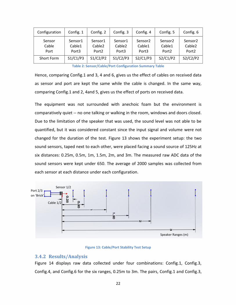
Configuration Config. 1 Config. 2 Config. 3 Config. 4 Config. 5 Config. 6
Sensor Cable Port
Sensor1 Cable1 Port3
Sensor1 Cable2 Port2
Sensor1 Cable2 Port3
Sensor2 Cable1 Port3
Sensor2 Cable1 Port2
Sensor2 Cable2 Port2
Short Form S1/C1/P3 S1/C2/P2 S1/C2/P3 S2/C1/P3 S2/C1/P2 S2/C2/P2
Table 2: Sensor/Cable/Port Configuration Summary Table
Hence, comparing Config.1 and 3, 4 and 6, gives us the effect of cables on received data
as sensor and port are kept the same while the cable is changed. In the same way,
comparing Config.1 and 2, 4and 5, gives us the effect of ports on received data.
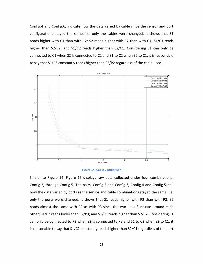
The equipment was not surrounded with anechoic foam but the environment is
comparatively quiet -- no one talking or walking in the room, windows and doors closed.
Due to the limitation of the speaker that was used, the sound level was not able to be
quantified, but it was considered constant since the input signal and volume were not
changed for the duration of the test. Figure 13 shows the experiment setup: the two
sound sensors, taped next to each other, were placed facing a sound source of 125Hz at
six distances: 0.25m, 0.5m, 1m, 1.5m, 2m, and 3m. The measured raw ADC data of the
sound sensors were kept under 650. The average of 2000 samples was collected from
each sensor at each distance under each configuration.
Figure 13: Cable/Port Stability Test Setup
3.4.2 Results/Analysis
Figure 14 displays raw data collected under four combinations: Config.1, Config.3,
Config.4, and Config.6 for the six ranges, 0.25m to 3m. The pairs, Config.1 and Config.3,
Speaker Ranges (m)
Sensor 1/2
Cable 1/2
Port 2/3
on ‘Brick’
23
Config.4 and Config.6, indicate how the data varied by cable since the sensor and port
configurations stayed the same, i.e. only the cables were changed. It shows that S1
reads higher with C1 than with C2; S2 reads higher with C2 than with C1; S1/C1 reads
higher than S2/C2; and S1/C2 reads higher than S2/C1. Considering S1 can only be
connected to C1 when S2 is connected to C2 and S1 to C2 when S2 to C1, it is reasonable
to say that S1/P3 constantly reads higher than S2/P2 regardless of the cable used.
Figure 14: Cable Comparison
Similar to Figure 14, Figure 15 displays raw data collected under four combinations:
Config.2, through Config.5. The pairs, Config.2 and Config.3, Config.4 and Config.5, tell
how the data varied by ports as the sensor and cable combinations stayed the same, i.e.
only the ports were changed. It shows that S1 reads higher with P2 than with P3; S2
reads almost the same with P2 as with P3 since the two lines fluctuate around each
other; S1/P2 reads lower than S2/P3; and S1/P3 reads higher than S2/P2. Considering S1
can only be connected to P2 when S2 is connected to P3 and S1 to C2 when S2 to C1, it
is reasonable to say that S1/C2 constantly reads higher than S2/C1 regardless of the port
0 0.5 1 1.5 2 2.5 3100
200
300
400
500
600
700
distance(m)
raw
data
Cable Comparison
Sensor1Cable1Port3
Sensor2Cable2Port2
Sensor1Cable2Port3
Sensor2Cable1Port2

24
used. The data difference based on ports is comparatively smaller than cables since the
dashed lines are closer to their corresponding solid lines in Figure 15 than in Figure 14.
Figure 15: Port Comparison
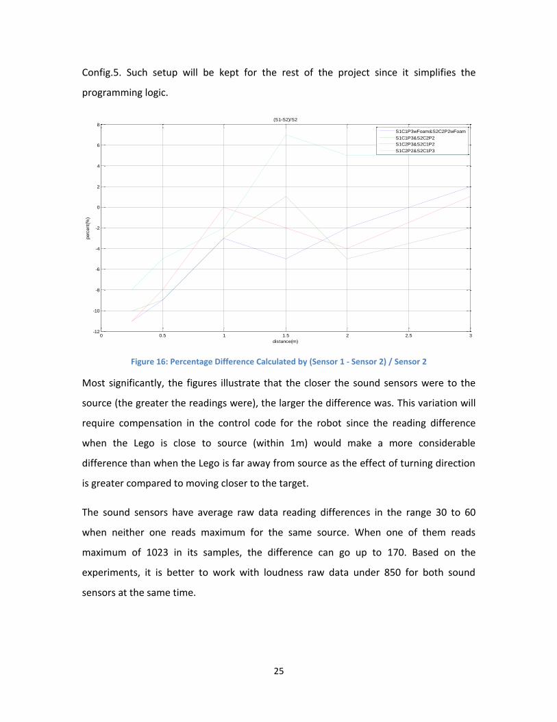
Figure 16 shows the percent difference between S1 and S2 in each of the following
cases: Config.1 and Config.6 surrounded with anechoic foam; Config.1 and Config.6
without foam; Config.3 and Config.5 without foam; Config.2 and Config.4 without foam.
The effect of anechoic foams was not significant as seen from Figure 16 after comparing
the blue line and the green one since they most of the time agree with each other on
which sensor reads higher within the 2.5m range. All four curves appear to share the
same characteristic: S1 reads much lower than S2 when the speaker was in close range
(<1m) no matter which cable or port it was connected to; and S1 started to read higher
when the speaker was in longer range.
The red line indicates that sensor 1 constantly reads smaller than or equal to sensor 2
when the sound source is in the range of 2.5m following the setup of Config.3 and
0 0.5 1 1.5 2 2.5 3100
150
200
250
300
350
400
450
500
550
600
distance(m)
raw
data
Port Comparison
Sensor1Cable2Port2
Sensor2Cable1Port3
Sensor1Cable2Port3
Sensor2Cable1Port2
25
Config.5. Such setup will be kept for the rest of the project since it simplifies the
programming logic.
Figure 16: Percentage Difference Calculated by (Sensor 1 - Sensor 2) / Sensor 2
Most significantly, the figures illustrate that the closer the sound sensors were to the
source (the greater the readings were), the larger the difference was. This variation will
require compensation in the control code for the robot since the reading difference
when the Lego is close to source (within 1m) would make a more considerable
difference than when the Lego is far away from source as the effect of turning direction
is greater compared to moving closer to the target.
The sound sensors have average raw data reading differences in the range 30 to 60
when neither one reads maximum for the same source. When one of them reads
maximum of 1023 in its samples, the difference can go up to 170. Based on the
experiments, it is better to work with loudness raw data under 850 for both sound
sensors at the same time.
0 0.5 1 1.5 2 2.5 3-12
-10
-8
-6
-4
-2
0
2
4
6
8
distance(m)
perc
ent(
%)
(S1-S2)/S2
S1C1P3wFoam&S2C2P2wFoam
S1C1P3&S2C2P2
S1C2P3&S2C1P2
S1C2P2&S2C1P3

26
Raw Data Range <170 [170, 200] [250, 450] [450,650]
Percent Reading Difference
(S1-S2)/S2 *100% -2.5% -0.3% -8% -11%
Table 3: Percent Difference Vs. Reading Range
As summarized in Table 3, based on the experimental data of the combination Config.3
and Config.5, when the raw data readings are over 450, S1 reads smaller than S2 on
average by 11% ((S2-S1)/S2); when in the range of [250, 450], S1 reads smaller than S2
by 8%; when in the range of over [170, 200], S1 reads smaller than S2 by 0.3%; when
below 170, S1 reads smaller than S2 by 2.5%. Adjustments of adding the difference in
non-moving situations onto S1’s reading would help minimize the error in decision
making due to sensor reading discrepancy. However, the calibration does not have to
use the exact numbers in the table and can vary from case to case since the two sensors
will be located apart from each other at a distance in the final design. The values will be
determined based on Lego’s performance and will be stated in the final test section.
3.5 Sound Sensor: Range Sensitivity According to Signals, Sound, and Sensation, the sound intensity from a point source will
obey the inverse square law if there are no reflections or reverberation, which says that
the intensity varies inversely as the square of the distance between the source and the
observer [15]. The speaker used here can be approximated as a point source. Therefore
theoretically the sound power emitted by the speaker should decrease according to the
inverse square law as the observer (sensor) moves away from the source. Here the Lego
sensors are tested to confirm that their measurements of the sound power correspond
with the inverse square law as they are moved further from the sound source.

27
3.5.1 Setup
The experimental setup for range sensitivity is the same as the previous Cable/Port
Stability experiments. The data from the last section is reused in this section but from a
different point of view. Instead of comparing pairs of data, we will look at all six sets of
data at the same time.
3.5.2 Results/Analysis
As stated in Chapter 2 where the Lego 9845 sound sensor was introduced, received
sound power is proportional to the raw ADC value squared. Hence, the collected raw
data are all squared and treated as unit-less sound power data before further
observations. For each of the six configurations, the power data were normalized to
start from 1 at 0.25m, i.e. Ir=0.25 =1, by dividing the power value at 0.25m. In theory,
without considering losses and noises, sound power should decrease proportional to the
inverse of range squared: , where is the received intensity at a certain
range , is the constant coefficient , is the emitted signal power, and is
the range between the sensor and the sound source [15]. For the normalized case, since
1, equals 0.252 and the equation is . In Figure 17, all six sets
of normalized data are plotted, as well as the reference curve , x∈
[0.25m, 3m]. All curves share the same characteristics, falling fast within the 1m range
and decreasing much slower from 1m to 3m. Also, the experimental values match the
reference curve fairly well within 1m. The reason why the curves do not decrease to a
point as low as the reference one is possibly due to the loss during the transmission, and
the ambient noise or the circuit noise. The sound Intensity detected by the Lego sensors
is consistent with the theoretical performance.

28
Figure 17: Normalized Sound Intensity
Figure 17 also shows that the Lego sound sensors’ best performance range is within
1.5m and they are not very sensitive when the range is 2m or further.
3.6 Ultrasonic Sensor: Measurement Accuracy Evaluate the accuracy of range measurements under various conditions when seeing a
surface that is not perfectly perpendicular to the ultrasonic sound’s travelling trace,
besides Lego’s official specification saying that the resolution of ultrasonic sensors is
1cm and the tolerance is +/- 3cm.
3.6.1 Fixed Range, Various Angles
Angled surfaces upset the ultrasonic sensor. Find out the workable range of angles to
get reasonable distance measurements.
3.6.1.a Setup

29
A cardboard box of dimensions 48cm-9cm-38cm was placed at three fixed distances
from the ultrasonic sensor: its front edge will be 38cm, 50cm and 150cm away from the
ultrasonic sensor’s transmitter and receiver end. When the box was in position 1, as
shown in Figure18, it was manually turned clockwise continuously but slowly until the
ultrasonic sensor cannot give valid readings, 255cm. Record the readings and the
corresponding angle at each change in the readings. For position 2 and 3, starting from
the perpendicular position, the cardboard box will be manually turned 10° at a time
clockwise till 90°, where the shorter edge of the box is facing the sensor. The average of
50 distance readings at each angle were recorded and analyzed.
Figure 18: Fixed range, various angles setup
3.6.1.b Results/Analysis
When the cardboard box was at position 1, the ultrasonic sensor reads 38cm away when
perpendicular. According to Figure 19, readings dropped to 37cm when the box was
tilted 11.5° clockwise facing the ultrasonic sensor; 36cm when tilted 22° and subject to
variations; 35cm when tilted 25°; to 34cm when tilted 30°. The distance reading stayed

30
at 34cm until the box was turned 36°, and the ultrasonic sensor was not able to give
valid distance measurements after 36°.
Figure 19: Readings at various angles, 38cm
For box position 2 and 3, the ultrasonic sensor’s distance readings vary as shown in Figure 20.
Both cases share the same characteristic that the greater the turning angle was, the worse the
distance reading was. The blue line shows that at a fixed distance of 50cm, the ultrasonic sensor
does not read valid distance for angles over 30°; the red one shows that at 150cm, it does not
read valid distance for angles over 20°.
Figure 20: Readings at various angles, 50cm and 150cm
0 10 20 30 40 50 6030
32
34
36
38
40
42
44
46
48
50
time(s)
range(c
m)
Object Range Vs. Time
0° 10° 20° 30° 40° 50° 60° 70° 80° 90°
average distance(50) 50 49.08 48 255 255 255 255 255 176.2 34
average distance(150) 149 149 255 255 255 184 255 255 255 255
0
50
100
150
200
250
300
Ran
ge (
cm)
Range Vs. Angle

31
34cm, the last reading at 90° for fixed distance of 50cm, is a result of the ultrasonic
sensor seeing the slim face on the box. A possible reason of the sensor not seeing it
when the fixed distance was 150cm is that this surface is so slim and far away from the
ultrasonic sensor that the receiver did not get the reflected transmitted signal.
An ultrasonic sensor does not read accurately when a surface is not perpendicular to the
way it is facing; the max angle of unreasonable readings decreases as the fixed distance
increases; and we can get reasonable readings only when the angle is less than 36°.
3.6.2 Fixed Angle, Various Ranges
Find out the accuracy of distance measurements when the ultrasonic sensor is looking
at a surface with a fixed angle.
3.6.2.a Setup
The Lego ultrasonic sensor was placed at a fixed angle facing the wall while the center of
the sensor was varied from 5cm to 50cm with 5cm increment away from the wall,
indicated in Figure 21. Two fixed angles were tested: 35° and 45°. The average of 100
data collected at each position will be analyzed.
Figure 21: Fixed angle, various ranges. Setup
32
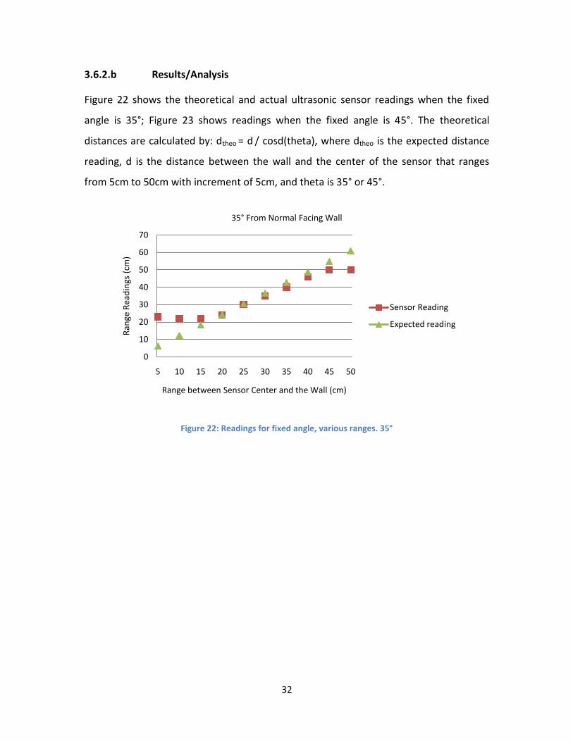
3.6.2.b Results/Analysis
Figure 22 shows the theoretical and actual ultrasonic sensor readings when the fixed
angle is 35°; Figure 23 shows readings when the fixed angle is 45°. The theoretical
distances are calculated by: dtheo = d / cosd(theta), where dtheo is the expected distance
reading, d is the distance between the wall and the center of the sensor that ranges
from 5cm to 50cm with increment of 5cm, and theta is 35° or 45°.
Figure 22: Readings for fixed angle, various ranges. 35°
0
10
20
30
40
50
60
70
5 10 15 20 25 30 35 40 45 50
Ran
ge R
ead
ings
(cm
)
Range between Sensor Center and the Wall (cm)
35°From Normal Facing Wall
Sensor Reading
Expected reading
33
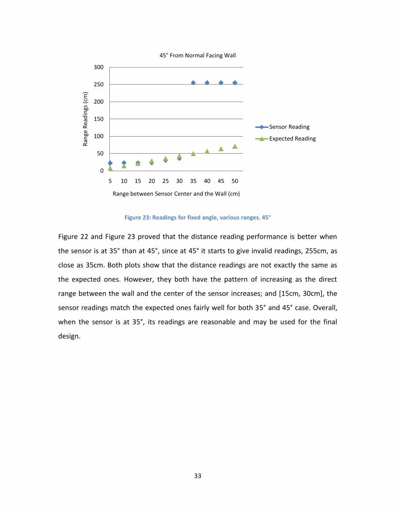
Figure 23: Readings for fixed angle, various ranges. 45°
Figure 22 and Figure 23 proved that the distance reading performance is better when
the sensor is at 35° than at 45°, since at 45° it starts to give invalid readings, 255cm, as
close as 35cm. Both plots show that the distance readings are not exactly the same as
the expected ones. However, they both have the pattern of increasing as the direct
range between the wall and the center of the sensor increases; and [15cm, 30cm], the
sensor readings match the expected ones fairly well for both 35° and 45° case. Overall,
when the sensor is at 35°, its readings are reasonable and may be used for the final
design.
0
50
100
150
200
250
300
5 10 15 20 25 30 35 40 45 50
Ran
ge R
ead
ings
(cm
)
Range between Sensor Center and the Wall (cm)
45°From Normal Facing Wall
Sensor Reading
Expected Reading

34
Chapter 4. Sound Source Seeking Robot
4.1 Objectives
The robot designed in this chapter will attempt to replicate the process of cognition and
decision making inside the female mating cricket’s nervous system. The robot will find
its way towards a sound source while avoiding possible obstacles without any external
aid or instruction, mimicking the female cricket seeking her mate. This chapter will cover
preparation experiments and analysis, the design of the Lego robot and the final robot
tests.
4.2 Required Hardware and Software
4.2.1 Software
The following software components were used during the development of the robot:
MATLAB R2011b;
The RWTH Mindstorms NXT MATLAB Toolbox, developed by members of the
RWTH Aachen University for educational purpose, is a free open source
product and is subject to the GNU GENERAL PUBLIC LICENSE;
The Phantom Lego NXT Driver, which allows the computer to communicate with
the Lego robot via an umbilical USB cable.
4.2.2 Hardware
Lego Components Used
One LEGO Mindstorms 9841 NXT Intelligent Brick with six AA batteries;
Two 9842 interactive servo motors;
Two 9845 sound sensors;
Four connection wires between motors/sensors and the brick;
One USB cable for PC/brick communication;
Other Hardware Components
One RadioShack Mini Audio Amplifier and a 9V battery;

35
A laptop running MATLAB2011b.
4.3 Direction Finding with the Sound Sensors Before deciding which way to turn, the robot must be able to perceive the direction
from which the sound originates. To model the anatomy of the cricket, two of the Lego
sound sensors were used to replicate the function of the insect’s antennae [3]. Here we
evaluate the ability of the Lego sensor to discern the sound source direction and
determine the design parameters for the final robot.
4.3.1 Objectives
To locate a sound source, the robot has to know the speaker position relative to itself.
This section will evaluate how well the pair of sound sensors can work to tell the
direction (left or right) from which a sound signal is coming. During the evaluating stage,
the minimum number of samples required and the order in which they are acquired will
be discovered; so that the true direction of the sound source can be identified.
4.3.2 Experiment Setup
The configuration of the hardware is shown in Figure 24.
Figure 24: Preparation Test Setup
The two sound sensors were 34cm apart end to end with the robot stationary. A sound
signal of 125Hz pure sine wave with constant volume was used and placed on a circle of
S1/C2/P3 S2/C1/P2
36
radius 1m or 2m centered at the midpoint of the two sensors. Sensor1/Cable2 was on
the left side, connected to port 3 of the NXT brick and Sensor2/Cable1 on the right to
port 2. The speaker is said to be in the front (90˚) when the line formed by the speaker
and the center is orthogonal to the line formed by the left and right sensor; left (180˚),
when both two sensors and the speaker are lined up and left one is closer; right (0˚),
when they are lined up and right one is closer. The speaker will be manually moved
around the circle with a 10˚ increment from 0˚ – 180˚ after samples have been recorded.
Since the sound sensors are omni-directional, see section 3.2, the performance of the
sensors at 180˚ – 360˚ can be predicted to be the same as 0˚ – 180˚. One buffer will be
used for each sensor to make sure that the data collected at each position are valid and
the comparison result of the two sensors is true to reality. The buffer size will be
discussed in the results section, as well as how the buffers are filled – fill the buffer for
one side first and then the other, or take one sample for one side and then the other
until the buffers have been filled. The results will show how accurate the sensors can tell
if the left or right sensor is closer to the sound source by comparing its data. However, it
is not able to tell whether the sound comes from its front or its back unless two more
sensors are used, one in the front and one in the back, according to the results from
section 3.2.
4.3.3 Results/Analysis
1m Radius, Buffer Size = 1000, Take 1 Sample for Left and Then Right Until the
Buffers Have Been Filled
Figure 25 shows the result when the speaker was on the circle of radius 1m and a buffer
size 1000 was used at each angle position. The average of the 1000 samples was
compared with the averages from other angles. No adjustment was made. The 0 – 90˚
section in Figure 25 was based on the raw data difference, sensor 2 subtracted by
sensor 1 (right-left); and the 90 – 180 degree section was based on the raw data
difference, sensor 1 subtracted by sensor 2 (left-right). Figure 25 shows that the average
of 1000 raw ADC data on the left is greater than the average on the right when the
speaker was actually sitting on the robot’s left (90˚ - 180˚); and vice versa when the

37
speaker was on right. The result also agrees with the previously discovered property
that sensor1 reads larger than sensor2 since the differences on the left are greater than
the differences on the right while the speaker volume was constant.
Figure 25: Raw Data Difference, 1000 samples Figure 26: Raw Data Difference, 80 samples
1m Radius, Buffer Size = 80, Take 1 Sample for Left and Then Right Until the
Buffers Have Been Filled
The only difference between Figure 25 and 26 is that the sensors used a buffer size of 80
in Figure 26. 80 is the lowest number of samples that the two sound sensors need to
collect in order to tell the correct direction of the sound source when the source is 1m
away. It was determined to be the lowest number of samples with which accurate
direction finding could be achieved. The minimum was arrived at by trying multiple
sample counts and evaluating the change in their performance.
Therefore, the sound sensors are able to tell if the sound source comes from the left or
right under the configuration of:
1) 34cm apart horizontally;
5
10
15
30
210
60
240
90
270
120
300
150
330
180 0
5
10
15
30
210
60
240
90
270
120
300
150
330
180 0

38
2) Taking at least 80 samples at a time;
3) The sound source is 1m away from the center of the two sensors;
4) Both the Lego and the source are standing still.
2m Radius, Buffer Size = 80, Take 1 Sample for Left and Then Right Until the
Buffers Have Been Filled
The same experiment setup (Figure 24) and procedure was repeated but the speaker
was moved around the 2m radius circle. Table 4 summarizes the averages of left and
right sensor data and their differences at all angle positions, using the same angle
notation as the setup in Figure 24. For angles [0˚, 90˚], the data differences are
calculated by right sound sensor data minus left sound sensor data; and vice versa for
[100˚, 180˚]. The results show that when the source is 2 meters away, 80 samples is not
enough to tell the correct direction because the left sensor started to return a larger
value than the right when the speaker was on the right at the 50˚ position ([50˚,90˚]),
and the results seemed random when the speaker was on the left.
Angle(˚) 0 10 20 30 40 50 60 70 80 90
Left Data 128 138 136 158 170 130 119 121 118 132
Right Data 139 146 142 160 172 124 119 125 112 122
Right – Left 11 8 6 2 2 -6 0 4 -6 -10
Direction Right Right Right Right Right Left Middle Right Left Left
Angle(˚) 100 110 120 130 140 150 160 170 180 Left Data 135 146 144 128 114 136 140 132 132 Right Data 121 144 146 133 110 139 139 127 135 Left – Right 14 2 -2 -5 4 -3 1 5 -3 Direction Left Left Right Right Left Right Left Left Right Table 4: Left and Right Data Differences Vs. Angles at 2m
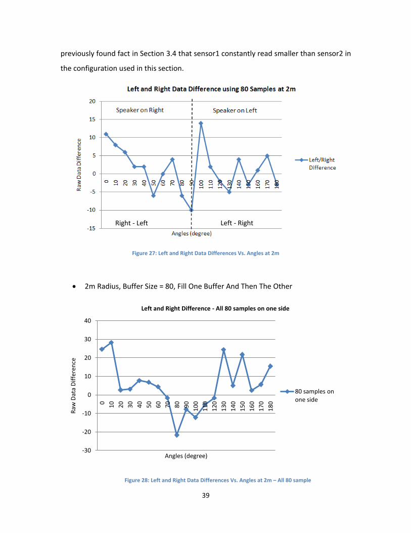
Figure 27 plots the left and right sensor data differences. Separated by dash line at 90˚,
it indicates that when the speaker is on the right side in [0˚, 40˚], the right sensor reads
greater than the left sensor and result in a correct direction finding; when the speaker is
on the left side, the sound data comparison results seem random. The reason why the
performance is better when the speaker is on the right side is possibly due to the
39
previously found fact in Section 3.4 that sensor1 constantly read smaller than sensor2 in
the configuration used in this section.
Figure 27: Left and Right Data Differences Vs. Angles at 2m
2m Radius, Buffer Size = 80, Fill One Buffer And Then The Other
Figure 28: Left and Right Data Differences Vs. Angles at 2m – All 80 sample
-30
-20
-10
0
10
20
30
40
0
10
20
30
40
50
60
70
80
90
10
0
11
0
12
0
13
0
14
0
15
0
16
0
17
0
18
0
Raw
Dat
a D
iffe
ren
ce
Angles (degree)
Left and Right Difference - All 80 samples on one side
80 samples on one side
Right - Left Left - Right
40
Results from this section are plotted in Figure 28, showing that taking all 80 samples on
one side at a time, instead of one on the left and one on the right, can increase the
accuracy for the setup in Figure 24. Figure 28 indicates an improvement in the direction
finding, compared to Figure 27, since on the right side, a correct direction is found for
angles [0˚, 60˚]; on the left, a correct direction is found for angles [130˚, 180˚]. Hence, in
the MATLAB code for the final design, program the sensors to take all samples on one
side before the other sensor starts sampling.
4.4 Sound Source Seeking Robot Design and Test
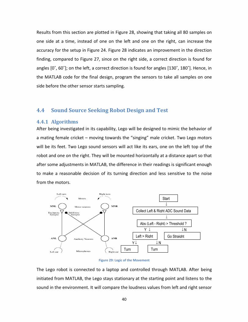
4.4.1 Algorithms
After being investigated in its capability, Lego will be designed to mimic the behavior of
a mating female cricket – moving towards the “singing” male cricket. Two Lego motors
will be its feet. Two Lego sound sensors will act like its ears, one on the left top of the
robot and one on the right. They will be mounted horizontally at a distance apart so that
after some adjustments in MATLAB, the difference in their readings is significant enough
to make a reasonable decision of its turning direction and less sensitive to the noise
from the motors.
Figure 29: Logic of the Movement
The Lego robot is connected to a laptop and controlled through MATLAB. After being
initiated from MATLAB, the Lego stays stationary at the starting point and listens to the
sound in the environment. It will compare the loudness values from left and right sensor
Start
Collect Left & Right ADC Sound Data
Abs (Left - Right) > Threshold ?
Go Straight Forward
Left > Right ?
Turn Right
Turn Left
↓
↓
↓ ↓
↓
↓
Y
Y
N
N
41
after some adjustment of calibration has been made on the raw data. Based on the
comparison result, the motors will rotate so that the Lego can turn left, right or go
straight. The 2-neuron system inside a female cricket is displayed on left in Figure 29 [3]
and the logic used to represent it in the MATLAB code is illustrated through the flow
chart in Figure 29. When the left sensor value is significantly higher than the right one,
the right wheel of the robot will rotate forward while the left wheel stays stationary for
the robot to turn left; and the reverse when the right sensor reads higher; both wheels
will rotate forward when the two loudness values are similar within a certain range.
After each turn, it will move forward a little bit and then stop and listen again.
Theoretically, the Lego robot will repeat that cycle over and over and be able to locate
the sound source while its center will face the source, given enough time. Furthermore,
it should be able to detour around possible obstacles without additional programming
or external aid due to the diffraction nature of waves.
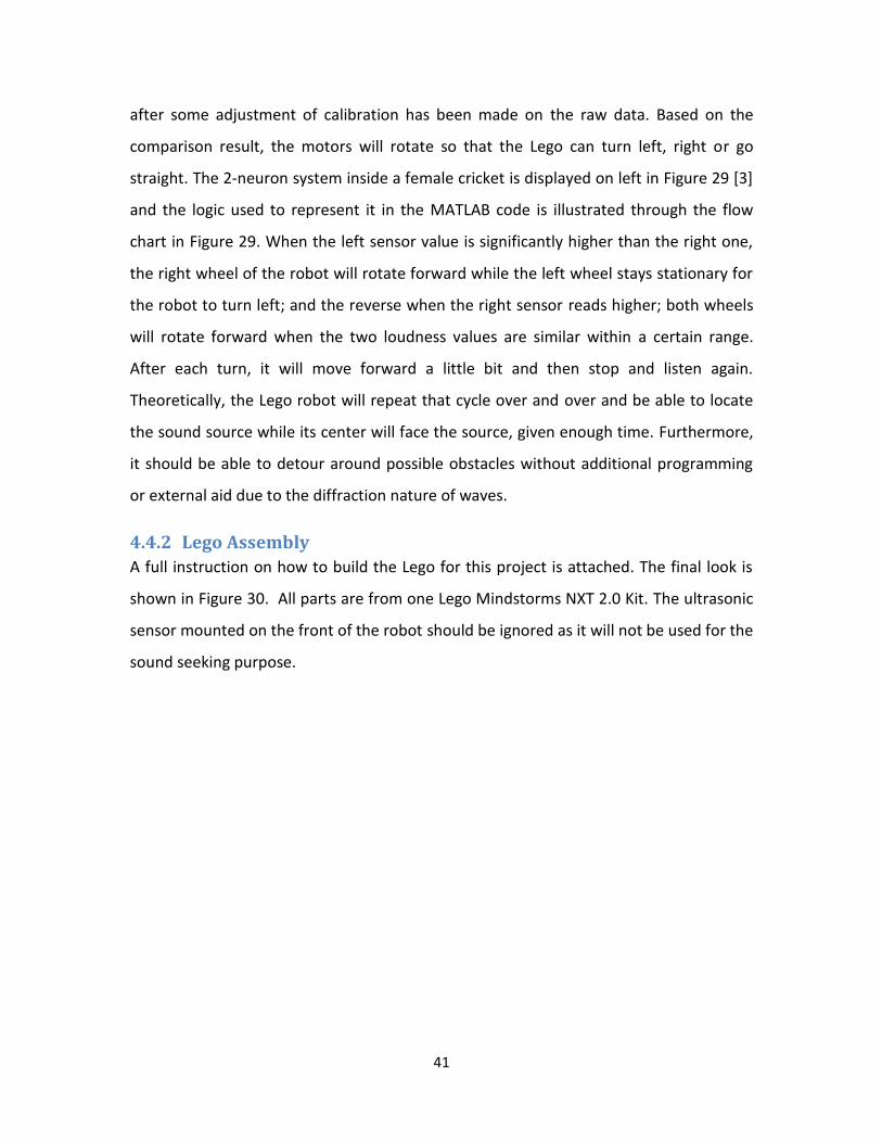
4.4.2 Lego Assembly
A full instruction on how to build the Lego for this project is attached. The final look is
shown in Figure 30. All parts are from one Lego Mindstorms NXT 2.0 Kit. The ultrasonic
sensor mounted on the front of the robot should be ignored as it will not be used for the
sound seeking purpose.
42
Figure 30: Final Lego Look
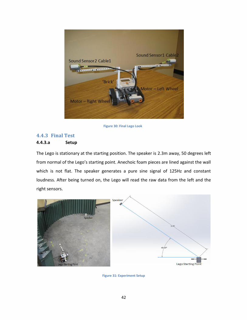
4.4.3 Final Test
4.4.3.a Setup
The Lego is stationary at the starting position. The speaker is 2.3m away, 50 degrees left
from normal of the Lego’s starting point. Anechoic foam pieces are lined against the wall
which is not flat. The speaker generates a pure sine signal of 125Hz and constant
loudness. After being turned on, the Lego will read the raw data from the left and the
right sensors.
Figure 31: Experiment Setup

43
Since left sensor (S1/C2/P3) constantly reads higher than the right one (S2/C1/P2)
(Section 3.4), the adjustment will be all on the left sensor data as illustrated in Figure 32.
When both data are under 190, the left raw data will be amplified by a factor of 1.11;
otherwise, when the sensor readings differ from each other by more than 20, the left
raw data will be amplified by a factor of 1.176 and no change will made to the raw data
in the other case.
Figure 32: Adjustment on Sensor Reading
After having determined the direction of the sound source with adjusted data, the Lego
will be moving in that direction, left, right or straight. When tested on the table surface,
the front center of the robot moved forward 8.0cm in the direction 46 degree left from
normal of its original location after each left turn command; forward 8.6 cm in the
direction 46 degree right from normal of its original location after each right turn
command; and straight forward 15.9cm after each go-straight command. Due to
different surface frictions, its movement might vary on the ground than on the table.
However, the result of being able to locate the sound source should stay the same.
The reception and reaction cycles will be repeated and eventually the Lego robot will
locate the speaker by standing exactly in front of it. Two cases will be tested with or
without an obstacle.
4.4.3.b Results/Analysis
The MATLAB program used was included in Appendix A.
No obstacle

44
When the area was clear of obstacles, the Lego robot moved to the speaker in 57
seconds with the blue route displayed in Figure 33 while the shortest route was the red
one. Lego wandered along the direct route and successfully located the speaker.
Figure 33: Lego Route Movement 1
One Obstacle
The second test scenario was with a box placed in the middle of its path while the
speaker and Lego’s starting position stayed the same. Figure 36 shows the route of the
Lego in blue when there was a Lego box in the middle of the direct route in red. Lego
used 63 seconds to locate and reach the speaker. It succeeded in detouring around the
box by steering to the right side of the box and then making a great left turn to the
speaker.

45
Figure 34: Experiment Setup Movement 2 Figure 35: Movement 2 Setup
Figure 36: Lego Route Movement 2

46
Chapter 5. Echoic Flow Theory This chapter will briefly cover the Echoic Flow theory inspired by echolocating bats and
the parameter developed in the theory. An approach to undertake echoic flow
calculations in MATLAB will also be explained.
5.1 What is Echoic Flow Optical flow was introduced by Gibson and developed by Lee and co-workers to explain
how humans and other members of the animal kingdom navigate complex
environments without having to compute and re-compute the position of all objects and
obstacles along with the position of self. Optical flow is a measure of changes in
received intensity regardless of source. Specifically, the parameter can be computed as
the ratio of intensity to a change in intensity over a given interval of time. Thus, the flow,
denoted represents the time for objects in relative motion to collide. Moreover, the
time derivative of , , is a measure of the intensity of that collision. The concept of
optical flow has been extended to both acoustic and echoic sensing and is sometimes
referred to as acoustic flow [15].
Dr. Graeme Smith and Prof. Baker, from The Ohio State University, have specifically
used the term echoic flow (EF) to represent active sensing systems that might use
acoustic or electromagnetic signals, and have developed the Echoic Flow theory for
radar sensing. Echoic flow may be formulated for different dimensions of measurement,
such as range or angle. Consider a simple and illustrative example of a radar application,
the associated with radial range is given by: where is the range to a
detected object and is the change in range of the object between the current and
previous measurements. is a direct measure of the time before collision and has
units of time.
5.2 Summary of Echoic Flow Collision Avoidance Simulation Dr. Smith and Prof. Baker’s paper includes a simulation which considers a vehicle
equipped with a monostatic radar system that is located inside a corridor formed from
of a series of point scatterers (shown in red, Figure 37) [8]. In Figure 37, “(a) shows a
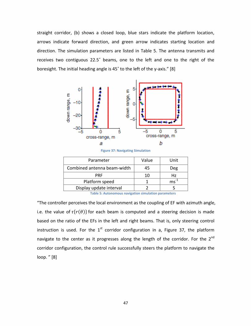
47
straight corridor, (b) shows a closed loop, blue stars indicate the platform location,
arrows indicate forward direction, and green arrow indicates starting location and
direction. The simulation parameters are listed in Table 5. The antenna transmits and
receives two contiguous 22.5˚ beams, one to the left and one to the right of the
boresight. The initial heading angle is 45˚ to the left of the y-axis.” [8]
Figure 37: Navigating Simulation
Parameter Value Unit
Combined antenna beam-width 45 Deg
PRF 10 Hz
Platform speed 1 ms-1
Display update interval 2 S Table 5: Autonomous navigation simulation parameters
“The controller perceives the local environment as the coupling of EF with azimuth angle,
i.e. the value of for each beam is computed and a steering decision is made
based on the ratio of the EFs in the left and right beams. That is, only steering control
instruction is used. For the 1st corridor configuration in a, Figure 37, the platform
navigate to the center as it progresses along the length of the corridor. For the 2nd
corridor configuration, the control rule successfully steers the platform to navigate the
loop. ” [8]

48
5.3 Measuring Tau using the Ultrasonic Sensor The ultrasonic sensor is intended to measure the range to an object. Here we describe
how, by processing the output of the sensor in MATLAB, it can be used to measure the
echoic flow parameter .
5.3.1 Objectives
The second demonstration robot will try to prove the Echoic Flow theory and realize
cases similar to Dr. Smith’s simulation [15], using Tau for steering control. We will use
Lego ultrasonic sensors to measure range and record the time at each measurement in
MATLAB to calculate Tau.
5.3.2 Taking Care of Ultrasonic Sensors’ Misreading
As having been described in Chapter 2, the Lego ultrasonic sensors return distance
measurements in cm in the range [-1, 255]. A valid measurement should be [0, 254cm]
while -1 means a misreading and 255 can be a misreading or an indication of the
maximum range. Besides the hardware problem, the distance reading can be wrong due
to multipath since the receiver on the sensor may use a wrong signal to calculate
distance, the signal that has been reflected from multiple surfaces instead of the one
that is reflected directly from the object that it should be seeing. We will find the most
effective way to get rid of the range misreading using a buffer.
Mean, median and mode (most frequent values in array) are three frequent commands
to use when smoothing data in MATLAB. A buffer size of 100 samples is randomly
selected and will be taken at each distance, 5cm to 200cm with 5cm increment, from
the ultrasonic sensor facing a wall perpendicularly. The average, median and mode of
the samples will be compared to the actual case.
Figure 38 shows the results from each buffer and the expected range measurement
values. All three of them work well and are almost the same when the ultrasonic sensor
is working within 100cm. For distances in [100cm, 160cm], in MATLAB, using mean
command for the 100 samples does smooth out the readings, but its results do not fit
the actual distances like median and mode. For distances over 160cm, all three of them

49
are not accurate, with a difference of over 50cm compared to the actual distance.
Therefore, the recommended working range is within 170cm for the final robot. Also,
the curves for median and mode are almost identical. A median filter is chosen to
estimate the true range, though a mode filter should work equally well.
Figure 38: Buffer Comparison
5.4 Calculating Tau A program will be written in MATLAB to calculate Tau, by , where is the
current range measurement, is the time interval between the previous range
measurement and the current one, and is the previous range measurement minus
the current one. Since is the first order estimate of velocity of the Lego, is the
same to be calculated by range over current velocity. The program included in Appendix
B follows the flow chart in Figure 39, nBufferSize will be the variable to control the
size of the median filter; rport is the port number on the Lego intelligent brick; Tick is
the counter for the buffer. The program will first set desired variables, get the first range
0 20 40 60 80 100 120 140 160 180 2000
50
100
150
200
250
300
Range (cm)
Range (
cm
)
Buffer Comparison
Mean
Median
Mode
Expected
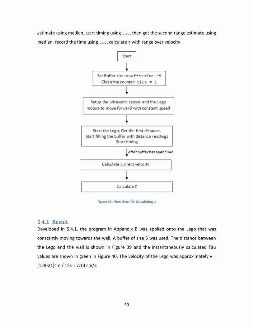
50
estimate using median, start timing using tic, then get the second range estimate using
median, record the time using toc, calculate with range over velocity .
Figure 39: Flow chart for Calculating
5.4.1 Result
Developed in 5.4.1, the program in Appendix B was applied onto the Lego that was
constantly moving towards the wall. A buffer of size 5 was used. The distance between
the Lego and the wall is shown in Figure 39 and the instantaneously calculated Tau
values are shown in green in Figure 40. The velocity of the Lego was approximately v =
(128-21)cm / 15s ≈ 7.13 cm/s.

51
Figure 39: Distance between Lego and the Wall
Based on the formula provided by Echoic Flow, a theoretical Tau value line is therefore
approximately , derived from seconds, where is the
estimated distant between the Lego and the wall, starting from 128cm (x=0) and ended
at 21cm (x=15s). The green line and the dash blue line in Figure 40 imply that the
calculated Tau values agree with the theoretical ones within a tolerance of +/- 3.8 sec.
The red line is the linear regression line of the calculated Tau line, . It
agrees with the theoretical Tau line with a tolerance less than 2 sec. Hence, the result of
the program is satisfying and the logic of the program will be used for the final design
for the collision avoidance robot.
0 2 4 6 8 10 12 14 1620
40
60
80
100
120
140
time(s)
range(c
m)
Object Range Vs. Time

52
Figure 40: Estimated Time before Collision of a Moving Lego
0 2 4 6 8 10 12 14 162
4
6
8
10
12
14
16
18
time(s)
tau(s
)
Estimated time before collision Vs. Time
y = - 0.89*x + 17
Instantaneously Calculated Tau
Linear Regression
Theoretical Tau
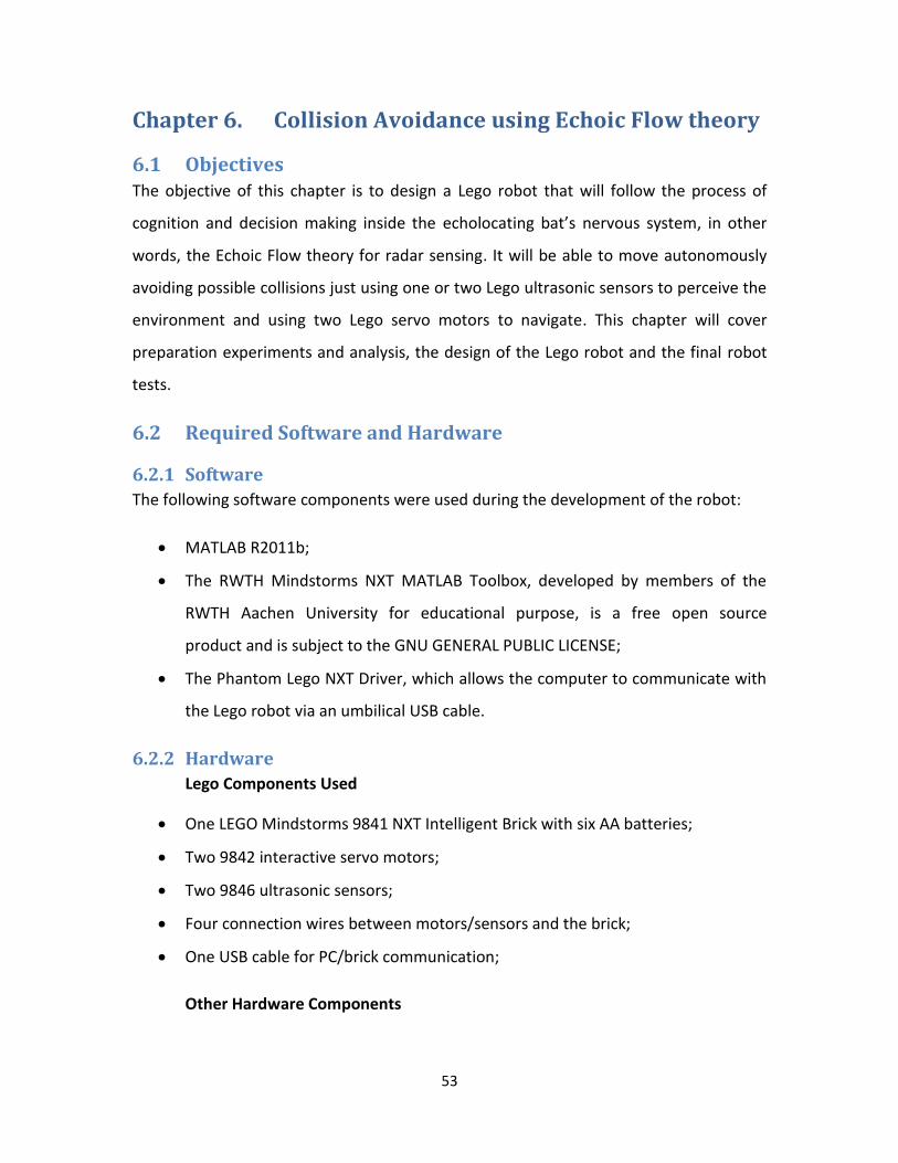
53
Chapter 6. Collision Avoidance using Echoic Flow theory
6.1 Objectives The objective of this chapter is to design a Lego robot that will follow the process of
cognition and decision making inside the echolocating bat’s nervous system, in other
words, the Echoic Flow theory for radar sensing. It will be able to move autonomously
avoiding possible collisions just using one or two Lego ultrasonic sensors to perceive the
environment and using two Lego servo motors to navigate. This chapter will cover
preparation experiments and analysis, the design of the Lego robot and the final robot
tests.
6.2 Required Software and Hardware
6.2.1 Software
The following software components were used during the development of the robot:
MATLAB R2011b;
The RWTH Mindstorms NXT MATLAB Toolbox, developed by members of the
RWTH Aachen University for educational purpose, is a free open source
product and is subject to the GNU GENERAL PUBLIC LICENSE;
The Phantom Lego NXT Driver, which allows the computer to communicate with
the Lego robot via an umbilical USB cable.
6.2.2 Hardware
Lego Components Used
One LEGO Mindstorms 9841 NXT Intelligent Brick with six AA batteries;
Two 9842 interactive servo motors;
Two 9846 ultrasonic sensors;
Four connection wires between motors/sensors and the brick;
One USB cable for PC/brick communication;
Other Hardware Components
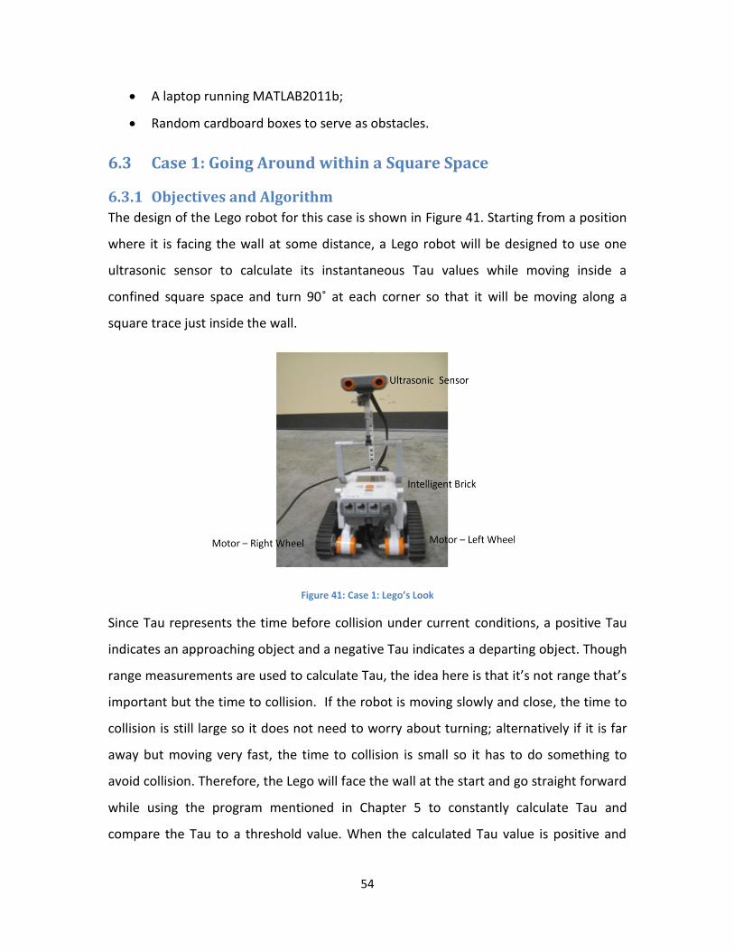
54
A laptop running MATLAB2011b;
Random cardboard boxes to serve as obstacles.
6.3 Case 1: Going Around within a Square Space
6.3.1 Objectives and Algorithm
The design of the Lego robot for this case is shown in Figure 41. Starting from a position
where it is facing the wall at some distance, a Lego robot will be designed to use one
ultrasonic sensor to calculate its instantaneous Tau values while moving inside a
confined square space and turn 90˚ at each corner so that it will be moving along a
square trace just inside the wall.
Figure 41: Case 1: Lego’s Look
Since Tau represents the time before collision under current conditions, a positive Tau
indicates an approaching object and a negative Tau indicates a departing object. Though
range measurements are used to calculate Tau, the idea here is that it’s not range that’s
important but the time to collision. If the robot is moving slowly and close, the time to
collision is still large so it does not need to worry about turning; alternatively if it is far
away but moving very fast, the time to collision is small so it has to do something to
avoid collision. Therefore, the Lego will face the wall at the start and go straight forward
while using the program mentioned in Chapter 5 to constantly calculate Tau and
compare the Tau to a threshold value. When the calculated Tau value is positive and

55
smaller than the threshold, the two Lego motors will cooperate with each other to turn
the robot 90˚ to the right; otherwise, it will keep going straight forward. After each turn,
it will repeat the process, going forward and turn right.
6.3.2 Setup
The Lego robot will be mounted with one ultrasonic sensor facing the front so that when
the robot is moving straight forward, the ultrasound transmitted is travelling in the
same direction, straight forward.
The Lego robot will be put into a 48cm-by 48cm square space approximately formed by
cardboard boxes and the wall, as illustrated in Figure 42.
Figure 42: Case 1: Lego’s Space
6.3.3 Results / Analysis
The Lego robot successfully performed the designed job of going forward and turning
right at a corner when the calculated Tau is smaller than a threshold value, for thirteen
consecutive corners/turnings. The MATLAB program for this task is included in Appendix
B. After a few tests, the threshold value for Tau is set to 0.8 sec for the robot not only to
avoid colliding into the wall and also have enough space (approximately 15cm) for
turning after each stop. Figure 43 displays the range readings (solid blue) and the
calculated Tau values (solid red) of the first four turns. In the shape of saw tooth, the
negative slopes of the solid blue line indicate that, repeated four times, the Lego robot
is approaching to a wall. The minimum points of the blue line indicate that the Lego

56
stops and turns when the distance to a wall is roughly 17cm. The Tau line is noisy but it
has the repetitive decreasing trend and whenever it reaches the 0.8 sec threshold (blue
dash line), it correctly corresponds to the position where the Lego is approaching to the
wall at roughly 17cm.
Figure 43: Case 1: Distance Measurements and Calculated Tau
Theoretically, the robot will be able to go along a square trace inside the space forever if
not terminated. Actually, the Lego motors’ limitation on turning angle leads to the
Lego’s incapability of making a perfect 90˚ turn. During the trial whose data are plotted
in Figure 43, the robot successfully made 13 turns at the corners before the
accumulated turning angle difference made the ultrasonic sensor face sideway to the
wall that it was next to instead of facing straight to the wall that it was approaching to.
0 50 100 150 200 250 300 3500
5
10
15
20
25
30
35
40
Sample number
Tau(s
ec)
Dis
tance(c
m)
Lego in Square Space
Tau
Distance
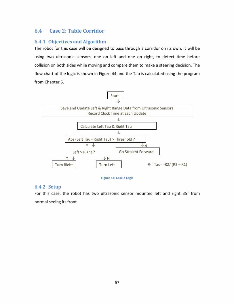
57
6.4 Case 2: Table Corridor
6.4.1 Objectives and Algorithm
The robot for this case will be designed to pass through a corridor on its own. It will be
using two ultrasonic sensors, one on left and one on right, to detect time before
collision on both sides while moving and compare them to make a steering decision. The
flow chart of the logic is shown in Figure 44 and the Tau is calculated using the program
from Chapter 5.
Figure 44: Case 2 Logic
6.4.2 Setup
For this case, the robot has two ultrasonic sensor mounted left and right 35˚ from
normal seeing its front.
Start
Save and Update Left & Right Range Data from Ultrasonic Sensors
Record Clock Time at Each Update
Abs (Left Tau - Right Tau) > Threshold ?
Go Straight Forward Left > Right ?
Turn Left Turn Right
↓
↓
↓ ↓
↓
↓
Y
Y
N
N
Calculate Left Tau & Right Tau
↓
Tau= -R2/ (R2 – R1) *dt.

58
Figure 45: Case 2 Lego’s Look
As explained in Chapter 3, the Lego ultrasonic sensors do not return correct distance
measurements when a surface is at an angle greater than 30˚ and the performance of
an ultrasonic sensor facing a 35˚ angled surface has been evaluated. To compensate the
angle problem, the corridor for the robot to pass through does not have two parallel
walls. Instead, the walls are sloped, as illustrated in Figure 46.
Figure 47: Case 2 Setup
6.4.3 Results / Analysis
The Lego robot successfully passed through the corridor without colliding into the walls.
The path taken by the robot during one trial is approximated and shown in Figure 48.
Ultrasonic Sensor 1 Ultrasonic Sensor 2
Motor – Left Wheel
Motor – Right Wheel
59
Figure 48: Case 2 Illustrative Lego route Figure 49: Case 2 Lego’s Distance Measurements
The distance measurements are shown in Figure 49. The ultrasonic sensors return
255cm when the transmitted ultrasound signal is not reflected back to the receiver or it
does see an open space beyond its maximum range of 255cm. The distance
measurements agree with the robot’s route. At first, the left sensor’s transmitted signal
was not reflected back to its receiver because of its angle to the left wall, while the right
sensor returned reasonable measurements. Both sensors returned reasonable
measurements as the robot is in the corridor. When the robot moved to the open end of
the corridor and at a position steered to the left, the right sensor detected the open
area outside the corridor while the left sensor still detected the left wall.
0 5 10 15 20 250
50
100
150
200
250
300Table Corridor
Ran
ge (
cm)
Number of Samples
Left
Right
33cm
65cm

60
Figure 50: Case 2 Lego’s Tau calculation
Eight turns were made by Lego to pass through the corridor and they are indicated on
Figure 50 whenever the absolute left and right Tau difference is greater than a threshold
of 0.8 sec. The -1000 sec is set when Lego gets a –inf for Tau. This is due to the
unchanged distance measurements collected by the Lego ultrasonic sensors and since
MATLAB does not like to compare a number to infinity, the value -1000 is used to
replace the –inf.
6.5 Case 3: The Autonomous Collision Avoidance Robots
6.5.1 Objectives and Algorithm
Use the exact same program as case 2 explained in section 6.4 on the Lego robot.
However, the robot is placed in an open space with randomly scattered objects. This will
test if the robot is able to autonomously navigate in the area without bumping into any
of the objects.

61
6.5.2 Setup
Objects are randomly placed on the lab floor, shown in Figure 51. Objects with smooth
and flat surfaces, such as metal and cardboard boxes, were used for the ultrasonic
sensors to make distance measurements as accurate as possible.
Figure 51: Case 3 Lab setup
6.5.3 Results
The Lego robot successfully navigated around the objects placed on the floor. In
addition, it is also able to navigate around a person whenever they stand on one side
(left or right) of the Lego in its front. Due to the fact that the two ultrasonic sensors are
mounted on top of the robot with 35˚ from normal left and right, the robot is not able
to avoid an object that is directly in front of it where neither one of the sensors can
detect it.
62
Chapter 7 Conclusion
7.1 Conclusion Despite the limitations from the Lego sensors and motors, the sound seeking robot and
the collision avoidance robot have performed well their designed functions. The two
robotic models have successfully proved the idea that a set of rules behind a complex
animal behavior can be very simple by demonstrating two different sensing systems and
behaviors using similar simple logics.
7.2 Wider Impact and Future Work This project has successfully illustrated that the Lego Mindstorms NXT robot is capable
of testing scientific theories. It is not ideal in every aspect such as module and
programming limitations, but it is powerful enough after the limitations are taken care
of. The approach of utilizing the “toy kit” offers a cheap and simple alternative to test
and evaluate simple cognitive sensing or intelligent control ideas before expensive large
scale or real-life testing.
In addition, the Echoic Flow theory for radar sensing is a newly developed theory and
the Lego robot designed in this project happened to be the very first one that uses
Echoic Flow for steering control. The results from the collision avoidance robot have
confirmed the potential of applying Echoic Flow to real-life applications, such as vehicles.
This is currently under study by the PhD student Mr. Saif Alsaif. Ideally, it is a candidate
for aiding systems so that a vehicle can autonomously navigate and avoid collisions.
With better equipment, a more accurate instantaneous time before collision can be
calculated and linked to the motors’ steering angle and power so that the robot will be
able to have smoother turns and a better performance as a result. Furthermore, utilizing
the coupled Tau’s from the Echoic Flow theory, Tau and the first derivative of Tau, onto
robots may lead to some more complex behaviors.
7.3 Regulatory Rules and Industry Standards This project is a pure lab-based research and during the development of this project,
since no live test subject was used, no regulatory rule or industrial standard was applied.

63
However, future applications of the results would need regulations since possible
applications may be on manmade vehicles like automotives and aircrafts as an aiding
system for steering control. In order to coordinate between different concerned groups,
e.g. between individuals and crafts, between crafts and other crafts, it will be necessary
to have regulations for at least two aspects. The first one is for traffic control so that the
communication between concerned groups is clear and smooth. The second is for
related equipment such as sensor and radar on its specifications because it might emit
signals that interfere with equipment for other uses. The complexity of the rules will be
depending on future engineers’ work.

64
Appendix A %%%%%move towards sound source COM_CloseNXT('all') close all clear all
clc
hNXT = COM_OpenNXT(); COM_SetDefaultNXT(hNXT);
%% Set up motors leftWheel = MOTOR_B; rightWheel = MOTOR_C; bothWheels = [leftWheel; rightWheel]; drivingPower = -60; turningPower = -50; drivingDist = 500; turningDist = 600; % in degrees backDist = 1500;
mTurnLeft2 = NXTMotor(rightWheel, 'Power', turningPower, 'TachoLimit',
turningDist); mTurnLeft2.SpeedRegulation = false; mTurnLeft2.ActionAtTachoLimit = 'Coast'; % the right-turn objects are the same, but mirrored: mTurnRight1 = NXTMotor(leftWheel, 'Power', turningPower, 'TachoLimit',
turningDist); mTurnRight1.SpeedRegulation = false; mTurnRight1.ActionAtTachoLimit = 'Coast';
mForward = NXTMotor(bothWheels, 'Power', drivingPower,'TachoLimit',
drivingDist); mForward.ActionAtTachoLimit = 'Coast';
OpenSound(SENSOR_2,'DB'); OpenSound(SENSOR_3,'DB'); rstatus = NXT_SetInputMode(SENSOR_2, 'SOUND_DB', 'RAWMODE',
'dontreply'); lstatus = NXT_SetInputMode(SENSOR_3, 'SOUND_DB', 'RAWMODE',
'dontreply');
right=zeros(1,200); left=zeros(1,200); lresampled=zeros(1,60); rresampled=zeros(1,60); rtime=zeros(1,200); ltime=zeros(1,200);
a=2; pause(5)

65
%% start while a<=60 tic for i= 1:200 right(i) = GetSound(SENSOR_2); rtime(i)=toc; end
tic for i=1:200 left(i)=GetSound(SENSOR_3); ltime(i)=toc; end rnewtime = linspace( rtime( 1 ), rtime( end ), 100 ); lnewtime = linspace( ltime( 1 ), ltime( end ), 100 ); rresampled(a) = mean(interp1( rtime, right,rnewtime)); lresampled(a) = mean(interp1( ltime, left,lnewtime));
%calibrattion if lresampled(a) >190 || rresampled(a) >190 l(a)=lresampled(a)/0.85; r(a)=rresampled(a); if l(a) - r(a) > 10 fprintf('Left.\n'); mTurnLeft2.SendToNXT(); pause(2) mTurnLeft2.Stop('brake')
elseif r(a) - l(a) > 10 fprintf('Right.\n'); mTurnRight1.SendToNXT(); pause(2) mTurnRight1.Stop('brake')
else fprintf('Straight.\n'); mForward.SendToNXT(); pause(2) mForward.Stop('brake') end
else l(a)=lresampled(a)/0.9; r(a)=rresampled(a); if l(a) - r(a) > 15 fprintf('Left.\n'); mTurnLeft2.SendToNXT(); pause(2) mTurnLeft2.Stop('brake')
elseif r(a) - l(a) > 15 fprintf('Right.\n'); mTurnRight1.SendToNXT(); pause(2)

66
mTurnRight1.Stop('brake')
else fprintf('Straight.\n'); mForward.SendToNXT(); pause(2) mForward.Stop('brake') end end
end a=a+1; fprintf('Straight.\n'); mForward.SendToNXT(); pause(2) mForward.Stop('brake')
%close sensors/motors StopMotor('all', 'off');
CloseSensor(SENSOR_2); CloseSensor(SENSOR_3);

67
Appendix B
nBufferSize = 5;
rport = SENSOR_4;
Tick = 1; r_a_fDistBuffer = zeros(1, nBufferSize);
% get the first range for i=1:nBuffersize
rechos(i)= GetUltrasonic(rport); end r_fOldRange = median(rechos(1,:)); % start timing tic
while 1>0
r_fDist= GetUltrasonic(rport); % Fill the buffer (FIFO) r_a_fDistBuffer( 2 : end ) = r_a_fDistBuffer( 1 : end - 1 ); r_a_fDistBuffer( 1 ) = r_fDist; % calculate Tau when buffer is filled if Tick >= nBufferSize % new range r_fRangeEstimate= median(r_a_fDistBuffer); % time duration tCurrentTime = toc; tTimeDelta = tCurrentTime- tOldTime; % left/right Tau's r_dis = r_fRangeEstimate; r_fSpeed= (r_fRangeEstimate - r_fOldRange)/tTimeDelta); r_tTau = - r_fRangeEstimate / r_fSpeed;
end
Tick = Tick + 1; end
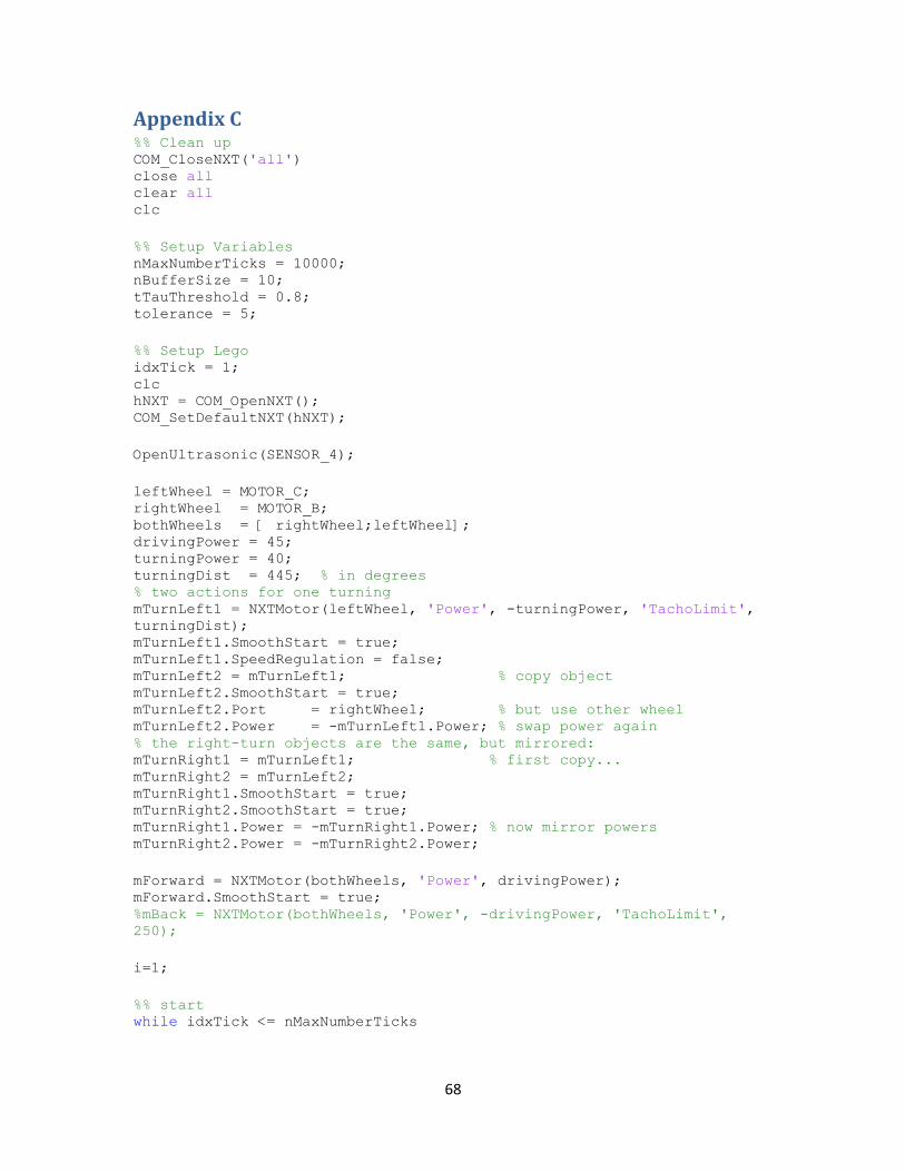
68
Appendix C %% Clean up COM_CloseNXT('all') close all clear all clc
%% Setup Variables nMaxNumberTicks = 10000; nBufferSize = 10; tTauThreshold = 0.8; tolerance = 5;
%% Setup Lego idxTick = 1; clc hNXT = COM_OpenNXT(); COM_SetDefaultNXT(hNXT);
OpenUltrasonic(SENSOR_4);
leftWheel = MOTOR_C; rightWheel = MOTOR_B; bothWheels = [ rightWheel;leftWheel]; drivingPower = 45; turningPower = 40; turningDist = 445; % in degrees % two actions for one turning mTurnLeft1 = NXTMotor(leftWheel, 'Power', -turningPower, 'TachoLimit',
turningDist); mTurnLeft1.SmoothStart = true; mTurnLeft1.SpeedRegulation = false; mTurnLeft2 = mTurnLeft1; % copy object mTurnLeft2.SmoothStart = true; mTurnLeft2.Port = rightWheel; % but use other wheel mTurnLeft2.Power = -mTurnLeft1.Power; % swap power again % the right-turn objects are the same, but mirrored: mTurnRight1 = mTurnLeft1; % first copy... mTurnRight2 = mTurnLeft2; mTurnRight1.SmoothStart = true; mTurnRight2.SmoothStart = true; mTurnRight1.Power = -mTurnRight1.Power; % now mirror powers mTurnRight2.Power = -mTurnRight2.Power;
mForward = NXTMotor(bothWheels, 'Power', drivingPower); mForward.SmoothStart = true; %mBack = NXTMotor(bothWheels, 'Power', -drivingPower, 'TachoLimit',
250);
i=1;
%% start while idxTick <= nMaxNumberTicks
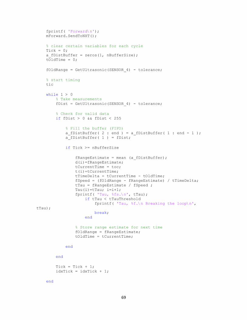
69
fprintf( 'Forward\n'); mForward.SendToNXT();
% clear certain variables for each cycle Tick = 0; a_fDistBuffer = zeros(1, nBufferSize); tOldTime = 0;
fOldRange = GetUltrasonic(SENSOR_4) - tolerance;
% start timing tic
while 1 > 0 % Take measurements fDist = GetUltrasonic(SENSOR_4) - tolerance;
% Check for valid data if fDist > 0 && fDist < 255
% Fill the buffer (FIFO) a_fDistBuffer( 2 : end ) = a_fDistBuffer( 1 : end - 1 ); a_fDistBuffer( 1 ) = fDist;
if Tick >= nBufferSize
fRangeEstimate = mean (a_fDistBuffer); d(i)=fRangeEstimate; tCurrentTime = toc; t(i)=tCurrentTime; tTimeDelta = tCurrentTime - tOldTime; fSpeed = (fOldRange - fRangeEstimate) / tTimeDelta; tTau = fRangeEstimate / fSpeed ; Tau(i)=tTau; i=i+1; fprintf( 'Tau, %fs.\n', tTau); if tTau < tTauThreshold fprintf( 'Tau, %f.\n Breaking the loop\n',
tTau); break; end
% Store range estimate for next time fOldRange = fRangeEstimate; tOldTime = tCurrentTime;
end
end
Tick = Tick + 1; idxTick = idxTick + 1;
end
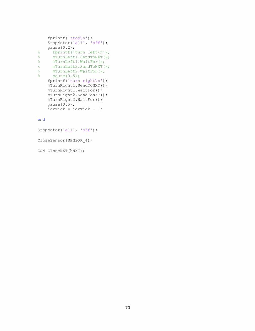
70
fprintf('stop\n'); StopMotor('all', 'off'); pause(0.2); % fprintf('turn left\n'); % mTurnLeft1.SendToNXT(); % mTurnLeft1.WaitFor(); % mTurnLeft2.SendToNXT(); % mTurnLeft2.WaitFor(); % pause(0.5); fprintf('turn right\n'); mTurnRight1.SendToNXT(); mTurnRight1.WaitFor(); mTurnRight2.SendToNXT(); mTurnRight2.WaitFor(); pause(0.5); idxTick = idxTick + 1;
end
StopMotor('all', 'off');
CloseSensor(SENSOR_4);
COM_CloseNXT(hNXT);

71
Appendix D %% Clean up COM_CloseNXT('all') close all clear all
%% Setup Variables nMaxNumberTicks = 10000; nBufferSize = 20; tTauThreshold = 0.8; tolerance = 0; tOldTime = 0;
%% Setup Lego idxTick = 1;
clc hNXT = COM_OpenNXT(); COM_SetDefaultNXT(hNXT);
lport = SENSOR_1; rport = SENSOR_4;
OpenUltrasonic(lport); OpenUltrasonic(rport);
leftWheel = MOTOR_B; rightWheel = MOTOR_C; bothWheels = [leftWheel; rightWheel]; drivingPower = -35; turningPower = -50; turnLeftDist = 150; % in degrees turnRightDist = 150; seeDist = 100; % two actions for one turning mTurnLeft1 = NXTMotor(leftWheel, 'Power', -turningPower, 'TachoLimit',
turnLeftDist); mTurnLeft1.SmoothStart = true; mTurnLeft1.SpeedRegulation = false; mTurnLeft2 = mTurnLeft1; % copy object mTurnLeft2.SmoothStart = true; mTurnLeft2.Port = rightWheel; % but use other wheel mTurnLeft2.Power = -mTurnLeft1.Power; % swap power % the right-turn objects are the same, but mirrored: mTurnRight1 = mTurnLeft1; mTurnRight1.TachoLimit = turnRightDist; mTurnRight2 = mTurnLeft2; mTurnRight1.SmoothStart = true; mTurnRight2.SmoothStart = true; mTurnRight1.Power = -mTurnRight1.Power; mTurnRight2.Power = -mTurnRight2.Power;
mForward = NXTMotor(bothWheels, 'Power', drivingPower); mForward.SmoothStart = true; mSee = mForward;

72
mSee.TachoLimit = seeDist;
counter = 0; % counter for Tau
%% start
while idxTick <= nMaxNumberTicks
% go forward mForward.SendToNXT();
% clear certain variables for each cycle Tick = 1; l_a_fDistBuffer = zeros(1, nBufferSize); r_a_fDistBuffer = zeros(1, nBufferSize);
% get the first pair of left and right ranges for i=1:10 lechos(i) = GetUltrasonic(lport); pause(0.005); rechos(i)= GetUltrasonic(rport); pause(0.005); end l_fOldRange = median(lechos(1,:)) - tolerance; r_fOldRange = median(rechos(1,:)) - tolerance;
% start timing tic
while 1 > 0
lechos = GetUltrasonic(lport); pause(0.005); rechos= GetUltrasonic(rport); pause(0.005); l_fDist = lechos - tolerance; r_fDist = rechos - tolerance;
% Check for valid data if l_fDist > -1 && l_fDist < 256 && r_fDist > -1 && r_fDist <
256 % Fill the buffer (FIFO) l_a_fDistBuffer( 2 : end ) = l_a_fDistBuffer( 1 : end - 1 ); l_a_fDistBuffer( 1 ) = l_fDist; r_a_fDistBuffer( 2 : end ) = r_a_fDistBuffer( 1 : end - 1 ); r_a_fDistBuffer( 1 ) = r_fDist;
% calculate Tau when buffer is filled if Tick >= nBufferSize counter = counter + 1;
% new ranges l_ranges (counter, :) = l_a_fDistBuffer; r_ranges (counter, :) = r_a_fDistBuffer;

73
l_fRangeEstimate= median (l_a_fDistBuffer); r_fRangeEstimate= median (r_a_fDistBuffer);
% time duration tCurrentTime(counter) = toc; tTimeDelta(counter) = tCurrentTime(counter) - tOldTime;
% tic toc errors if tTimeDelta(counter) < 0
fprintf('Negative time
duration: %0.2f.\n',tTimeDelta(counter)); tTimeDelta(counter) = tTimeDelta(counter-1);
end
% left/right Tau's r_dis(counter) = r_fRangeEstimate; l_dis(counter) = l_fRangeEstimate; l_fSpeed(counter) = (l_fRangeEstimate - l_fOldRange ) /
tTimeDelta(counter); l_tTau(counter) = - l_fRangeEstimate /
l_fSpeed(counter) ; r_fSpeed(counter) = (r_fRangeEstimate - r_fOldRange ) /
tTimeDelta(counter); r_tTau(counter) = - r_fRangeEstimate /
r_fSpeed(counter);
% Store old data for next time if it does not BREAK l_fOldRange = l_fRangeEstimate; r_fOldRange = r_fRangeEstimate; tOldTime = tCurrentTime(counter);
% set -1000 to all inf if r_tTau(counter) == -inf r_tTau(counter) = -1000; end
if l_tTau(counter) == -inf l_tTau(counter) = -1000; end
if abs(abs( l_tTau(counter)) - abs(r_tTau(counter))) >
tTauThreshold
fprintf('Left %0.2f s\nRight %0.2f
s\n',l_tTau(counter), r_tTau(counter)); fprintf('stop\n'); StopMotor('all', 'off'); break;
end

74
end
end
Tick = Tick + 1; idxTick = idxTick + 1; end
% after break/stop, turn to the smaller Tau
side if r_tTau(counter) < l_tTau(counter)
fprintf('turn right\n'); mTurnRight2.SendToNXT(); mTurnRight2.WaitFor(); mTurnRight1.SendToNXT(); mTurnRight1.WaitFor(); mSee.SendToNXT(); mSee.WaitFor(); pause(0.5);
else
fprintf('turn left\n'); mTurnLeft1.SendToNXT(); mTurnLeft1.WaitFor(); mTurnLeft2.SendToNXT(); mTurnLeft2.WaitFor(); mSee.SendToNXT(); mSee.WaitFor(); pause(0.5);
end
end
StopMotor('all', 'off');
CloseSensor(lport); CloseSensor(rport);
COM_CloseNXT(hNXT);
75
References
1. Y. Wang, Y. Wang, S. Patel, & D. Patel. A layered reference model of the brain
(LRMB). IEEE Transactions on Systems, Man, and Cybernetics (C),Vol. 36, No. 2,
pp. 124-133, 2004.
2. B. Webb. Robots. Photograph. Cricket Lab.
http://homepages.inf.ed.ac.uk/bwebb/cricket/. Web. 19 March 2013.
3. B. Webb. Using robots to model animals: a cricket test. Robotics and
Autonomous Systems, Vol. 16, Issues 2-4, pp.117-134, 1995.
4. J.J. Gibson. The Perception of the Visual World. Boston: Houghton Mifflin. 1950.
5. D. N. Lee, J. a Simmons, P. a Saillant, and F. Bouffard. “Steering by
echolocation: a paradigm of ecological acoustics.” Journal of comparative
physiology. A, Sensory, neural, and behavioral physiology Vol. 176, No.3, pp. 347-
54, 1995.
6. B. Kolb, and I. Q. Whishaw. Introduction to Brain and Behavior. 3rd ed. Worth
Publishers. 2009. pp.337-339.
7. K. Ghose, T. K. Horiuchi, P. S. Krishnaprasad, and C. F. Moss. Echolocating Bats
Use a Nearly Time-Optimal Strategy to Intercept Prey. [Online]. Available:
http://www.plosbiology.org/article/info%3Adoi%2F10.1371%2Fjournal.pbio.004
0108.
8. Smith, Graeme E., and Baker, Christopher J., “Echoic flow for radar and sonar”.
ELECTRONICS LETTERS. Vol.48, No.18, pp. 1160 – 1161, 2012.
9. RWTH - Mindstorms NXT Toolbox for MATLAB. http://www.mindstorms.rwth-
aachen.de/trac.
10. Lego Mindstorms NXT Intelligent Brick. http://shop.lego.com/en-US/NXT-Intelligent-
Brick-9841.
11. Lego Mindstorms Interactive Servo Motor. http://shop.lego.com/en-US/Interactive-
Servo-Motor-9842.
12. Lego Mindstorms Sound Sensor. http://shop.lego.com/en-US/Sound-Sensor-9845.
13. Lego Mindstorms Ultrasonic Sensor. http://shop.lego.com/en-US/Ultrasonic-Sensor-
9846.
14. Aswin. “The Ultrasonic Sensor”. NXT Time.
http://nxttime.wordpress.com/2012/09/12/the-ultrasonic-sensor/.
15. Hartmann, William M. Signals, Sound, and Sensation. Woodbury, NY: American
Institute of Physics. 1997. pp.36.