HAL Id: hal-01883208https://hal.archives-ouvertes.fr/hal-01883208

Submitted on 27 Sep 2018

HAL is a multi-disciplinary open accessarchive for the deposit and dissemination of sci-entific research documents, whether they are pub-lished or not. The documents may come fromteaching and research institutions in France orabroad, or from public or private research centers.

L’archive ouverte pluridisciplinaire HAL, estdestinée au dépôt et à la diffusion de documentsscientifiques de niveau recherche, publiés ou non,émanant des établissements d’enseignement et derecherche français ou étrangers, des laboratoirespublics ou privés.

Complete symmetry classification and compact matrixrepresentations for 3D strain gradient elasticity

Nicolas Auffray, Qi-Chang He, Hung Le Quang

To cite this version:Nicolas Auffray, Qi-Chang He, Hung Le Quang. Complete symmetry classification and compactmatrix representations for 3D strain gradient elasticity. International Journal of Solids and Structures,Elsevier, 2019, 159, pp.197-210. hal-01883208

COMPLETE SYMMETRY CLASSIFICATION AND COMPACTMATRIX REPRESENTATIONS FOR 3D STRAIN GRADIENT

ELASTICITY

N. AUFFRAY, Q.C. HE, AND H. LE QUANG

Abstract. Strain Gradient Elasticity (SGE) is now often used in mechanics and physics,owing to its capability to model some non-classical phenomena, such as size effects, inmaterials and structures. However, certain fundamental questions about it have not yetreceived complete responses. In its linear setting, the constitutive law of SGE is charac-terized by a fourth-order elasticity tensor, a fifth-order one and a sixth-order one. Evenif the matrix representations for the 3D fourth- and sixth-order elasticity tensors areavailable for all possible symmetry classes, the counterparts for the 3D fifth-order tensor,whose presence is unavoidable for materials with non-centrosymmetric microstructure,are still lacking. In addition, although the symmetry classes for each of the fourth-, fifth-and sixth-order elasticity tensor spaces are known, the symmetry classes for these tensorspaces as a whole have never been reported and clarified in the literature. The presentwork solves these two fundamental problems preventing the full understanding and ex-ploitation of the linear constitutive law of SGE. Precisely, the matrix representations ofthe fifth-order tensor for all of its 29 symmetry classes are provided in a compact andwell-structured way. Further, linear SGE is shown to possess 48 symmetry classes, andfor each of these symmetry classes, the matrix representations of its fourth-, fifth- andsixth-order tensors are now available.

1. Introduction

In its classical (or standard) setting, continuum mechanics [Truesdell and Toupin, 1960,Truesdell and Noll, 1965] resorts only to the first displacement gradient in describing de-formations. Even if this simple geometrical (or kinematical) framework is satisfactoryin most situations of practical interest for classical bulk materials and at the usual en-gineering scale, its validity for emergent materials becomes questionable. For example,consequent electric polarization can be induced even in non-piezoelectric nanomaterialsdue to high strain-gradients. This phenomenon, known as flexoelectricity, cannot be mod-elled in the realm of classical continuum mechanics [Cross, 2006, Le Quang and He, 2011,Zubko et al., 2013, Yvonnet and Liu, 2017]. Another example concerns architecturedmaterials whose microstructure spans several scales [Brechet and Embury, 2013]. Thislack of scale separation prohibits the use of classical continuum mechanics in their overallmacroscopic description. Last, but not least, specific microstructures can be designed tomaximize higher order effects. The pantographic architecture is a well-known exampleof such a situation [dell’Isola and Steigmann, 2015, dell’Isola et al., 2016]. For the lastdecade, non-standard effects in architectured materials have been experimentally and nu-merically evidenced [Alibert et al., 2003, Liu et al., 2012, Liu and Hu, 2016, Bacigalupoand Gambarotta, 2014a,b, 2017, Rosi and Auffray, 2016, Poncelet et al., 2018, Reda et al.,2018]. Two examples of such non-classical effects occurring in architectured materials areillustrated on the figures below. The first example, investigated by Rosi and Auffray

Date: September 27, 2018.2000 Mathematics Subject Classification. 74B05, 15A72.Key words and phrases. Anisotropy, Symmetry classes, Strain-gradient elasticity, Chirality, Non centro

symmetry.1

[2016], consists in the time domain analysis of the propagation of a shear pulses in ahoneycomb lattice. On Figure 1 the total displacement is depicted for two pulse havingdifferent spectral contents. For a low frequency pulse, the propagation is isotropic (Figure1a) while for a high frequency pulse the propagation becomes anisotropic (Figure 1b)

(a) Low Frequency pulse (b) High Frequency pulse

Figure 1. Propagation of a shear pulse in a honeycomb lattice. Totaldisplacement is displayed.

The second example is a numerical experiement extracted from Poncelet et al. [2018].In this experiment a sample having a non-centrosymmetric inner architecture is loadedin uniaxial tension. The resulting displacement fields are depicted on Figure 2a andFigure 2b. The result shows a flexure-like displacement superimposed to the classicalelongation. Such a behaviour reveals that, due to the non-centro symmetric unit cell,a coupling between the stress and the strain-gradient takes place within the sample.The aforementioned two effects are scale-depend and tend to vanish as the unit cell sizedecreases with respect to the sample one.

ux(mm)

(a) Displacement field ux forZπ2 pattern

uy(mm)

(b) Displacement field uy forZπ2 pattern

Figure 2. Displacement fields under 1 N uniform tensile force along x-direction for a non centrosymmetric pattern specimen.

For the continuum modelling of the aforementioned emergent materials, two optionsare at hand: (a) to remain in the realm of classical continuum mechanics by explicitly

2

describing the complex microstructure; (b) to get rid of the microstructure by incorpo-rating its effects into a non-standard continuum formulation. From the numerical pointof view, and especially for optimization perspectives, the option (a) is often prohibitivelyexpensive. The option (b), belonging to what is called Generalized Continuum Mechanics[Maugin, 2010], is the route here chosen because it is much less costly.

The first Strain-Gradient Elasticity (SGE) proposed by Mindlin [1964] is among themost important generalized continuum theories. In its linear setting, the infinitesimalstrain tensor ε and its gradient η = ε⊗∇ are linearly related to the second-order Cauchystress tensor σ and the third-order hyperstress tensor τ by Equation 1 where a fourth-order tensor C, a fifth-order tensor M and a sixth-order tensor A are involved and verifythe index permutation symmetry properties specified in Equation 2. In the foregoing ex-amples, the sixth-order tensor A is involved in the continuum description of the hexagonalwave propagation (c.f. Figure 1), while the fifth-order one M intervenes in the couplingbetween stress and strain-gradient (c.f. Figure 2).

The fourth-order tensor C defines the conventional elastic properties of a material.Its study had experienced a long history [Love, 1944] before a complete understandingwas achieved quite recently [Boehler et al., 1994, Forte and Vianello, 1996, Olive et al.,2017]. Concerning the fifth- and sixth-order tensors, M and A, their investigation werefar from being complete. In addition, studies in strain-gradient elasticity had been almostexclusively focused on isotropic materials and their extension to anisotropic materials isquite recent [Auffray et al., 2009, 2013, 2015, Lazar and Po, 2015, Placidi et al., 2016,Mousavi et al., 2016, Yaghoubi et al., 2017, Reda et al., 2018]. First results were obtainedin the 2D context by Auffray et al. [2009] who derived all anisotropic matrices of A; theseresults were then extended to M [Auffray et al., 2015].

The 3D case is far more complex. A first result was given by dell’Isola et al. [2009]who provided an explicit matrix representation of the isotropic sixth-order tensor A. Pa-panicolopulos [2011] investigated features of the tensor M with respect to the symmetrygroup SO(3) (hemitropic). Some analytical solutions to problems of hemitropic (SO(3)-invaraint) strain-gradient elasticity have been obtained by Iesan [2013, 2014], Iesan andQuintanilla [2016]. But the classification of anisotropic systems was absent. In Oliveand Auffray [2013, 2014a], theoretical results about the number and types of symmetryclasses for A and M in 3D were obtained. It is hence know that the space of sixth-ordertensors A is divided into 17 different symmetry classes, while the space of fifth-order ten-sors M is partitioned into 29 different symmetry classes. The matrix representations ofthe sixth-order tensor A for all its symmetry classes were specified for the first time byAuffray et al. [2013] in a compact and well-structured way. These matrix representationshave been shown to be useful for analysing the results of higher-order homogenization inarchitectured materials [Bacigalupo and Gambarotta, 2014a], understanding wave prop-agation in lattice materials [Bacigalupo and Gambarotta, 2014b, Rosi and Auffray, 2016]and, more recently, determining second order elasticity by molecular dynamics [Admalet al., 2017]. Note also that simplified anisotropic constitutive laws have recently beenproposed in [Polizzotto, 2017, 2018].

In SGE, the fifth-order coupling tensor M of a material is null or non-null accordingas its microstructure is centro-symmetric or not [Lakes and Benedict, 1982, Lakes, 2001].In the 3D case, the complete matrix representations of M are still unknown. In 3D,apart from the work of Papanicolopulos [2011] and Iesan and Quintanilla [2016], little hasbeen done about the strain-gradient elasticity of materials with non-centro-symmetricmicrostructure. However, as proved by Boutin [1996] via asymptotic analysis, the effectof M may be dominant over the one of A. In statics, some recent experiments on anarchitectured beam [Poncelet et al., 2018] have evidenced the necessity of involving M in

3

modelling its overall behaviour. Further, M is necessary to modelling interesting physicalphenomena of materials with non-centro-symmetric microstructure. In dynamics, thecoupling described by M induces changes in wave polarization and is associated to theacoustic activity of crystals and to so-called gyrotropic effects Toupin [1962], Portigal andBurstein [1968], Maranganti and Sharma [2007].

A comprehensive understanding of C (resp. A) is available in the sense that the definiteanswers to the following three fundamental questions have been provided: (i) How manysymmetry classes and which symmetry classes has C (resp. A)? (ii) For every givensymmetry class, how many independent material parameters has C (resp. A)? (iii) Foreach given symmetry class, what is the explicit matrix form of C (resp. A) relative to anorthonormal basis? At the present time, answers to questions (i) and (ii) concerning thestatic M tensor and its dynamic counterpart M? are available while the explicit matrixrepresentations of M and M? have not been provided so far. For practical applications,the last lacking result is the most important one.

In the present work, attention will be focused on studying the fifth-order coupling ten-sor M in the context of strain-gradient elastostatics. Questions related to its dynamiccounterpart M? constitute an independent study and the answers to them are postponedto another contribution. The present paper aims at obtaining the explicit matrix rep-resentations of M for all its 29 symmetry classes in a compact and well-structured way.As will be seen, the complexity and richness of M make that a proper solution to thisproblem is not straightforward at all.

The matrices obtained in the present work for the fifth-order tensor M complementthose for the classical fourth-order tensor C and the sixth-order tensor A by Auffrayet al. [2013]. The combination of these different results leads to the important conclusionthat there are exactly 48 different symmetry classes for 3D gradient-strain elasticity. Thisnumber means that SGE is much more complex and richer than the classical elasticitywhich has only 8 classes of symmetry. Finally, the results of this work allow us to havecompact and well-structured matrix representations of C, M and A for each of the possiblesymmetry classes.

The next sections of the paper are organized as follows. In section 2, the constitutive lawof strain gradient elasticity is recalled. The section 3 is devoted to introducing the mostimportant concepts concerning symmetry classes in O(3) and to recapitulating theoremsabout the symmetry classes of M obtained by Olive and Auffray [2014a]. The mainresults of the present work are given in section 4 and section 5. In section 4, the explicitmatrix representations of M for its 29 symmetry classes are provided in a compact andwell-structured form. The matrix representations of M are presented in such a mannerthat they can be directly used without resorting to group theory. In section 5, the resultsobtained in the present paper are combined with those of Auffray et al. [2013] for the sixth-order elasticity tensor A. It follows from this combination that there exists 48 symmetryclasses in O(3) for linear strain gradient elasticity. In section 6, a few concluding remarksare drawn.

There may be two ways to read this paper. If one likes to know not only the main resultsof the paper but also how to obtain them, the whole paper should be read. If one likesjust to know and use the main results of the paper but is not necessarily interested in theway of obtaining them, section 3 can be skipped, apart from the symmetry class notationsand the simple geometrical figures giving a physical interpretation of them, subsection 4.1and all the appendices can also skipped.

4

1.1. Notations. Throughout this paper, the Euclidean space E3 is equipped with a Carte-sian coordinates system associated to an orthonormal basis B = e1, e2, e3. Concerningnotation, the following convention is retained:

• Blackboard fonts will denote tensor spaces : T;• Tensors of order > 1 will be denoted using uppercase Roman Bold fonts : T;• Vectors will be denoted by lowercase Roman Bold fonts : t.

The following matrix spaces will be used:

• M(n) is the n2-D space of n dimensional square matrices ;• M(n,m) is the nm-D space of n×m rectangular matrices.

The orthogonal group in R3 is defined as O(3) = Q ∈ GL(3)|QT = Q−1, in whichGL(3) denotes the set of invertible transformations acting on R3. The following elementsof O(3) will be used in this study:

• Q a generic orthogonal transformation;• R(v; θ) ∈ O(3) the rotation about v ∈ R2 through an angle θ ∈ [0; 2π);• Pn ∈ O(3)\SO(3) the reflection through the line normal to n (Pn = 1− 2n⊗ n).

2. Strain-Gradient Elasticity

In this section, the constitutive law of Strain Gradient Elasticity (SGE) is introduced.In this introduction neither the momentum equation, nor the boundary conditions willbe detailed. The readers interested in these points can refer to the following referencesfor a more detailed presentation [Mindlin, 1964, Mindlin and Eshel, 1968, Germain, 1973,dell’Isola et al., 2009, Bertram, 2016].

In SGE the constitutive law gives the symmetric Cauchy stress tensor σ and the hy-perstress tensor τ in terms of:

• the infinitesimal strain tensor ε;• the strain-gradient tensor η = ε⊗∇ which, using index notation, reads ηijk = εij,k

with the comma denoting derivation.

Recall that ε and σ are second order symmetric tensors, while η and τ are third ordertensors symmetrical with respect to permutation of their first two indices. The constitutivelaw is specified by

σij = Cijlmεlm +Mijlmnηlmn,

τijk = Mlmijkεlm + Aijklmnηlmn.(1)

Above,

• C is the classical fourth-order elastic tensor;• M is the fifth-order coupling elastic (CE) tensor;• A is the sixth-order elastic (SOE) tensor.

These tensors satisfy the following index permutation symmetries:

C(ij) (lm) ; M(ij)(kl)m ; A(ij)k (lm)n (2)

where (..) stands for the minor symmetries whereas .. symbolises the major one. Theassociated vector spaces are defined accordingly:

Ela := C ∈ ⊗4(R3)|C(ij) (lm) , M := M ∈ ⊗5(R3)|M(ij)(kl)m , A := A ∈ ⊗6(R3)|A(ij)k (lm)n

As a consequence the strain gradient elastic behaviour is characterized by a triplet oftensors

L = (Cijkl,Mijklm, Aijklmn) ∈ Ela×M× A.5

The space of strain gradient elastic tensors is hence defined as

Sgr = Ela×M× A.Until now, Ela and A, the vector spaces of C and A, have been investigated, both in the

2D and 3D cases [Mehrabadi and Cowin, 1990, Forte and Vianello, 1996, Auffray et al.,2009, 2013]. The answers to the following three questions have been provided:(a) How many symmetry classes and which symmetry classes do Ela and A have?(b) For every given symmetry class, how many independent material parameters do Elaand A possess?(c) For each given symmetry class, what are the explicit matrix forms of C and A relativeto an adapted orthonormal basis?

In the 2D case, for Ela, He and Zheng [1996] demonstrated that the space of classicalfourth-order tensors is partitioned into 4 classes. This result was also obtained in adifferent way by Vianello [1997]. For A the question was solved in 2D by Auffray et al.[2009], the space of sixth-order tensors is more complex since it is divided into 8 classes.The space M has been studied recently in 2D [Auffray et al., 2015, 2016], and shown tobe divided into 6 classes.

In the 3D situation, the number of symmetry classes increases importantly since Elais now divided into 8 classes [Forte and Vianello, 1996], and A into 17 classes [Olive andAuffray, 2013, Auffray et al., 2013]. At the present time, these questions remain openfor the fifth-order tensor space in 3D. Some theoretical results are available [Olive andAuffray, 2014b, Auffray, 2013], but without explicit construction. In order to have acomplete anisotropic SGE theory, answering the aforementioned three questions for M isindispensable.

3. Symmetry classes

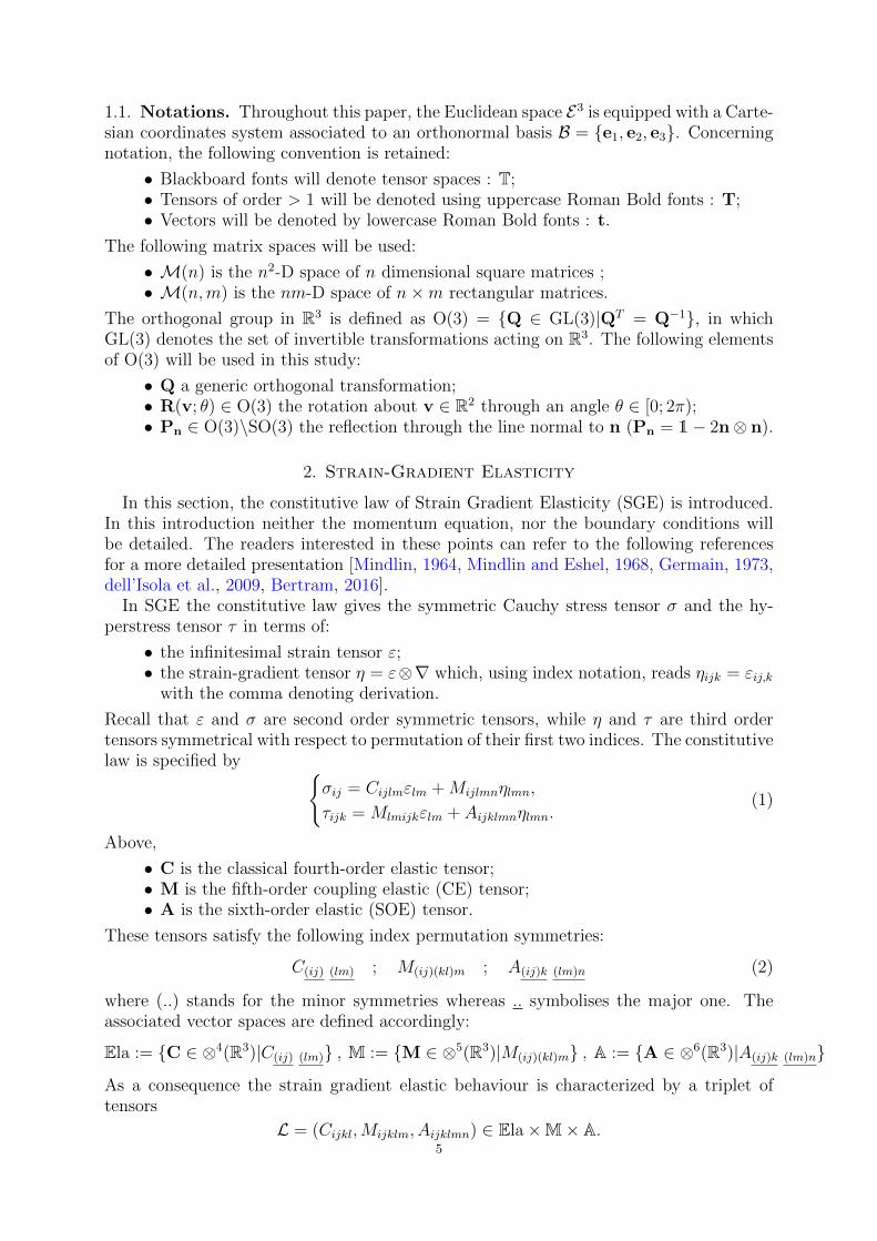
3.1. Material symmetry & Physical symmetry. Let consider a body as a compactsubset D0 of E3 having a microstructureM attached to any of its material points P ∈ D0.Those points are located with respect to a reference frame (R). The microstructure de-scribes the local organisation of the matter at scales below the one used for the continuousdescription (see Figure 3). As discussed in section 2 the elastic behaviour is assumed tobe described at the macrolevel by a SGE constitutive law formulated by Equation 1.

Figure 3. What is hidden below a material point

As for crystals, microstructures can possess invariance properties with respect to or-thogonal transformations Q ∈ O(3). Hence at each material point P , the set of such

6

transformations forms a point group GM(P ) ⊆ O(3) which describes the local materialsymmetries, formally

GM(P ) := Q ∈ O(3), Q · M(P ) =M(P )At the continuous macroscopic scale the detailed description of the microstructure islost, and information on the microstructure is contained in GM(P ). In the case of anhomogeneous medium the point dependence vanishes and GM(P ) = GM. This hypothesisof material homogeneity will be assumed for the rest of the paper.

Linear constitutive laws are encoded by tensors. For strain-gradient linear elasticity,the behaviour is described by a triplet of tensors L = (C,M,A). As the material elementis transformed by a punctual isometry Q, the physical property of the strain gradientelastic material is defined by another triplet L? = (C?,M?,A?). The link between thetwo set of tensors is given by:

C?ijkl = QioQjpQkqQlrCopqr;

M?ijklm = QioQjpQkqQlrQmsMopqrs;

A?ijklmn = QioQjpQkqQlrQmsQntAopqrst.

The notion of physical symmetry group has to be introduced. The symmetry group of Lis defined as1:

GL = GA ∩GM ∩GC. (3)

In which GC := Q ∈ O(3)|QioQjpQkqQlrCopqr = Cijkl;GM := Q ∈ O(3)|QioQjpQkqQlrQmsMopqrs = Mijklm;GA := Q ∈ O(3)|QioQjpQkqQlrQnsQmtAopqrst = Aijklmn.

The link between these two notions is given by the Curie principle which states thatthe material symmetry group (cause) is included in the physical symmetry group (conse-quence):

GM ⊆ GC

More details concerning this principle can be be found in Zheng and Boehler [1994].

3.2. Symmetry group and symmetry class. Let Q be an element of the 3D orthog-onal group O(3). A fifth-order tensor M is said to be invariant under the action of Q ifand only if

QioQjpQkqQlrQmsMopqrs = Mijklm. (4)

The symmetry group of M is defined as the subgroup GM of O(3) constituted of all theorthogonal transformations leaving M invariant2

GM = Q ∈ O(3) |QioQjpQkqQlrQmsMopqrs = Mijklm. (5)

Physically, the operations contained in O(3) are:

1It should be noted that an apparently different definition is provided for the symmetry group of astrain-gradient material by Bertram [2016]. Their definition is, in fact, more general since isochoric trans-formations preserving the elastic energy are considered. But, once restricted to isometric transformations,their definition coincides with ours.

2In odd dimension, the inversion belongs to the symmetry group of all even-order tensors, hencethe problem can be reduced to SO(3). This is why in [Forte and Vianello, 1996, Auffray et al., 2013]the classification of symmetry has been made with respect to SO(3). In the present situation the fullorthogonal group has to be considered. The link between the two classifications is as follows, if [H] is thesymmetry class of an even order tensor with respect to SO(3), its symmetry class with respect to O(3)will be [H ⊕ Zc2], with Zc2 denoting the group associated to the inversion operation.

7

• rotations (proper transformations of determinant 1), such elements form a sub-group SO(3) of the full orthogonal group;• mirrors and inversion (improper transformations of determinant -1).

As proposed by Forte and Vianello [1996] two fifth-order tensors M and N exhibitssymmetries of the same kind if and only if their symmetry groups are conjugate in thesense that

∃Q ∈ O(3),GN = QGMQT . (6)

Thus, the symmetry class [GM] of M corresponding to the conjugacy class of GM in O(3)is defined by

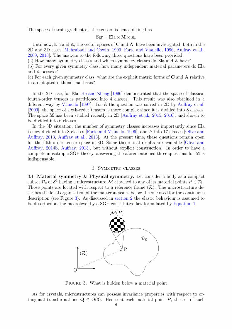
[GM] = G ⊆ O(3)|G = QGMQT , Q ∈ O(3). (7)

In other words, the symmetry class of M corresponds to its symmetry group modulo itsorientation. This idea is illustrated Figure 4.

Figure 4. Figures A and B have different but conjugate symmetry groups.Hence they belong to the same symmetry class.

To carry out the classification of odd order tensors, we should, in a first time, de-scribe the O(3)-closed subgroups. Throughout this paper, mathematical group notationswill be used; the equivalence between this system and the classical crystallographic ones(Hermann-Mauguin, Schoenflies) is recapitulated in Appendix B.

3.3. O(3)-closed subgroups. Classification of O(3)-closed subgroups is a classical theo-rem that can be found in many references (see, e.g., [Ihrig and Golubitsky, 1984, Sternberg,1994]):

Lemma 3.1. Every closed subgroup of O(3) is conjugate to one group of the followinglist, which has been divided into three classes:

I. Closed subgroups of SO(3).II. K := K ⊕ Zc2, where K is a closed subgroup of SO(3) and Zc2 = 1,−1;

III. Closed subgroups neither comprising −1 nor contained in SO(3).

Above, 1 denotes the identity transformation, and −1 stands for the inversion transfor-mation with respect to the origin.

In words, the subgroups of Type I consist of only rotations while those of Type IIcontain in addition the inversion (or central symmetry)3. The type III subgroups containsymmetry planes but theirs combinations do not generate the inversion4. Before detailingthe structure of classes, let us make a terminologic remark. A subgroup will be said to be

Centrosymmetric: if it contains the inversion; hence the subgroups of Type IIsubgroups are centrosymmetric;

3Type II subgroups also contain symmetry planes, but their constitutive feature is to possess theinversion.

4As soon a group possesses three mutual orthogonal symmetry planes it possesses the inversion.8

Chiral: if all its operations are orientation-preserving; hence those of Type I arechiral;

Polar: if it contains a single rotational axis; polar subgroups can be found in TypeI and Type III subgroups.

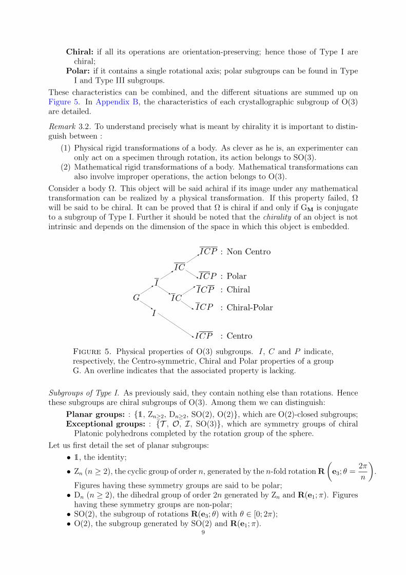
These characteristics can be combined, and the different situations are summed up onFigure 5. In Appendix B, the characteristics of each crystallographic subgroup of O(3)are detailed.

Remark 3.2. To understand precisely what is meant by chirality it is important to distin-guish between :

(1) Physical rigid transformations of a body. As clever as he is, an experimenter canonly act on a specimen through rotation, its action belongs to SO(3).

(2) Mathematical rigid transformations of a body. Mathematical transformations canalso involve improper operations, the action belongs to O(3).

Consider a body Ω. This object will be said achiral if its image under any mathematicaltransformation can be realized by a physical transformation. If this property failed, Ωwill be said to be chiral. It can be proved that Ω is chiral if and only if GM is conjugateto a subgroup of Type I. Further it should be noted that the chirality of an object is notintrinsic and depends on the dimension of the space in which this object is embedded.

Figure 5. Physical properties of O(3) subgroups. I, C and P indicate,respectively, the Centro-symmetric, Chiral and Polar properties of a groupG. An overline indicates that the associated property is lacking.

Subgroups of Type I. As previously said, they contain nothing else than rotations. Hencethese subgroups are chiral subgroups of O(3). Among them we can distinguish:

Planar groups: : 1, Zn≥2, Dn≥2, SO(2), O(2), which are O(2)-closed subgroups;Exceptional groups: : T , O, I, SO(3), which are symmetry groups of chiral

Platonic polyhedrons completed by the rotation group of the sphere.

Let us first detail the set of planar subgroups:

• 1, the identity;

• Zn (n ≥ 2), the cyclic group of order n, generated by the n-fold rotation R

(e3; θ =

2π

n

).

Figures having these symmetry groups are said to be polar;• Dn (n ≥ 2), the dihedral group of order 2n generated by Zn and R(e1; π). Figures

having these symmetry groups are non-polar;• SO(2), the subgroup of rotations R(e3; θ) with θ ∈ [0; 2π);• O(2), the subgroup generated by SO(2) and R(e1; π).

9

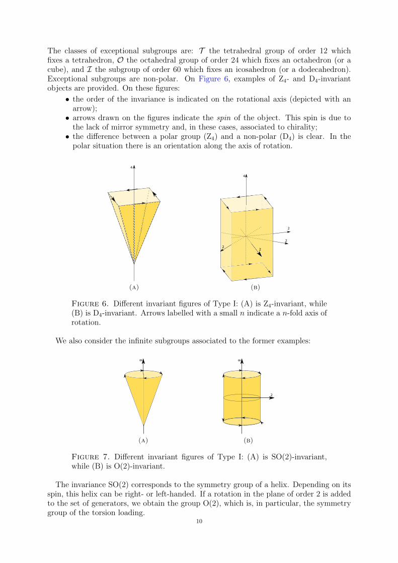
The classes of exceptional subgroups are: T the tetrahedral group of order 12 whichfixes a tetrahedron, O the octahedral group of order 24 which fixes an octahedron (or acube), and I the subgroup of order 60 which fixes an icosahedron (or a dodecahedron).Exceptional subgroups are non-polar. On Figure 6, examples of Z4- and D4-invariantobjects are provided. On these figures:

• the order of the invariance is indicated on the rotational axis (depicted with anarrow);• arrows drawn on the figures indicate the spin of the object. This spin is due to

the lack of mirror symmetry and, in these cases, associated to chirality;• the difference between a polar group (Z4) and a non-polar (D4) is clear. In the

polar situation there is an orientation along the axis of rotation.

4

(a)

4

2

2

22

(b)

Figure 6. Different invariant figures of Type I: (A) is Z4-invariant, while(B) is D4-invariant. Arrows labelled with a small n indicate a n-fold axis ofrotation.

We also consider the infinite subgroups associated to the former examples:

8

(a)

8

2

(b)

Figure 7. Different invariant figures of Type I: (A) is SO(2)-invariant,while (B) is O(2)-invariant.

The invariance SO(2) corresponds to the symmetry group of a helix. Depending on itsspin, this helix can be right- or left-handed. If a rotation in the plane of order 2 is addedto the set of generators, we obtain the group O(2), which is, in particular, the symmetrygroup of the torsion loading.

10

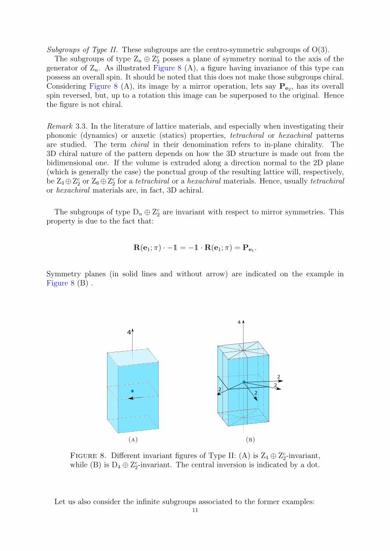
Subgroups of Type II. These subgroups are the centro-symmetric subgroups of O(3).The subgroups of type Zn ⊕ Zc2 posses a plane of symmetry normal to the axis of the

generator of Zn. As illustrated Figure 8 (A), a figure having invariance of this type canpossess an overall spin. It should be noted that this does not make those subgroups chiral.Considering Figure 8 (A), its image by a mirror operation, lets say Pe2 , has its overallspin reversed, but, up to a rotation this image can be superposed to the original. Hencethe figure is not chiral.

Remark 3.3. In the literature of lattice materials, and especially when investigating theirphononic (dynamics) or auxetic (statics) properties, tetrachiral or hexachiral patternsare studied. The term chiral in their denomination refers to in-plane chirality. The3D chiral nature of the pattern depends on how the 3D structure is made out from thebidimensional one. If the volume is extruded along a direction normal to the 2D plane(which is generally the case) the ponctual group of the resulting lattice will, respectively,be Z4⊕Zc2 or Z6⊕Zc2 for a tetrachiral or a hexachiral materials. Hence, usually tetrachiralor hexachiral materials are, in fact, 3D achiral.

The subgroups of type Dn ⊕ Zc2 are invariant with respect to mirror symmetries. Thisproperty is due to the fact that:

R(e1; π) · −1 = −1 ·R(e1; π) = Pe1 .

Symmetry planes (in solid lines and without arrow) are indicated on the example inFigure 8 (B) .

4

(a)

4

2

2

22

(b)

Figure 8. Different invariant figures of Type II: (A) is Z4 ⊕ Zc2-invariant,while (B) is D4 ⊕ Zc2-invariant. The central inversion is indicated by a dot.

Let us also consider the infinite subgroups associated to the former examples:11

8

(a) (b)

Figure 9. Different invariant figures of Type II: (A) is SO(2) ⊕ Zc2-invariant, while (B) is O(2)⊕ Zc2-invariant.

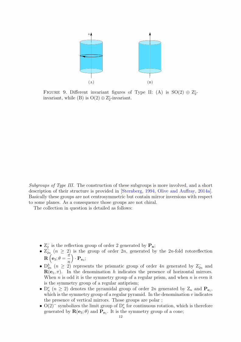
Subgroups of Type III. The construction of these subgroups is more involved, and a shortdescription of their structure is provided in [Sternberg, 1994, Olive and Auffray, 2014a].Basically these groups are not centrosymmetric but contain mirror inversions with respectto some planes. As a consequence those groups are not chiral.

The collection in question is detailed as follows:

• Z−2 is the reflection group of order 2 generated by Pn;• Z−2n (n ≥ 2) is the group of order 2n, generated by the 2n-fold rotoreflection

R(e3; θ =

π

n

)·Pe3 ;

• Dh2n (n ≥ 2) represents the prismatic group of order 4n generated by Z−2n and

R(e1, π). In the denomination h indicates the presence of horizontal mirrors.When n is odd it is the symmetry group of a regular prism, and when n is even itis the symmetry group of a regular antiprism;• Dv

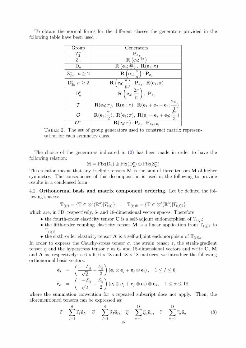
n (n ≥ 2) denotes the pyramidal group of order 2n generated by Zn and Pe1 ,which is the symmetry group of a regular pyramid. In the denomination v indicatesthe presence of vertical mirrors. Those groups are polar ;• O(2)− symbolizes the limit group of Dv

n for continuous rotation, which is thereforegenerated by R(e3; θ) and Pe1 . It is the symmetry group of a cone;

12

4

(a)

4

(b)

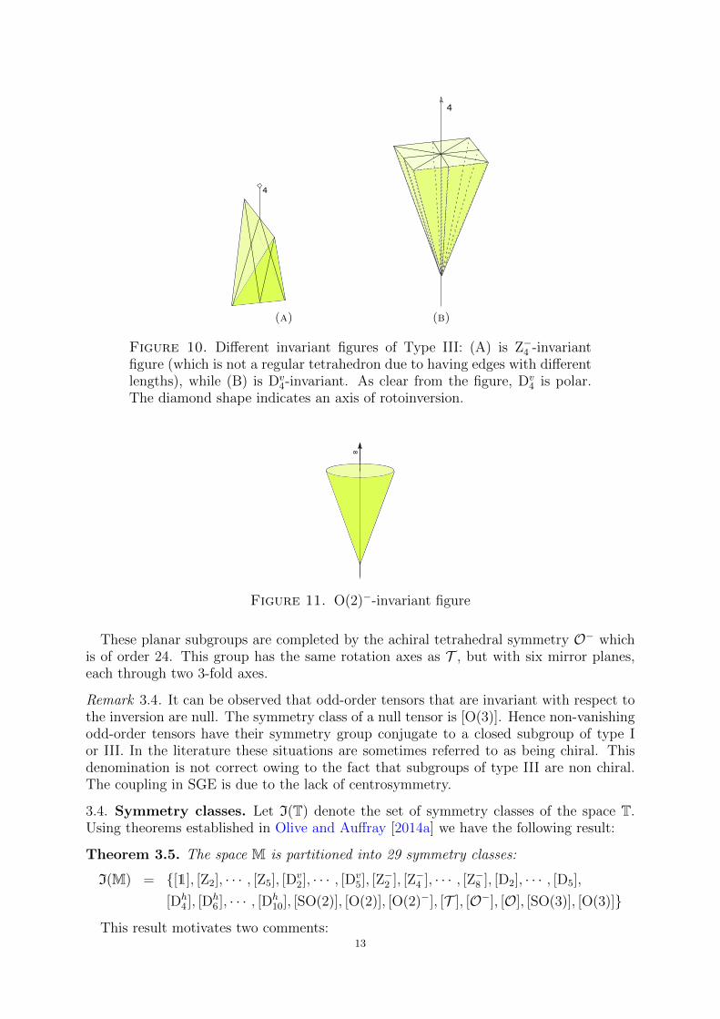
Figure 10. Different invariant figures of Type III: (A) is Z−4 -invariantfigure (which is not a regular tetrahedron due to having edges with differentlengths), while (B) is Dv

4-invariant. As clear from the figure, Dv4 is polar.

The diamond shape indicates an axis of rotoinversion.

8

Figure 11. O(2)−-invariant figure

These planar subgroups are completed by the achiral tetrahedral symmetry O− whichis of order 24. This group has the same rotation axes as T , but with six mirror planes,each through two 3-fold axes.

Remark 3.4. It can be observed that odd-order tensors that are invariant with respect tothe inversion are null. The symmetry class of a null tensor is [O(3)]. Hence non-vanishingodd-order tensors have their symmetry group conjugate to a closed subgroup of type Ior III. In the literature these situations are sometimes referred to as being chiral. Thisdenomination is not correct owing to the fact that subgroups of type III are non chiral.The coupling in SGE is due to the lack of centrosymmetry.

3.4. Symmetry classes. Let I(T) denote the set of symmetry classes of the space T.Using theorems established in Olive and Auffray [2014a] we have the following result:

Theorem 3.5. The space M is partitioned into 29 symmetry classes:

I(M) = [1], [Z2], · · · , [Z5], [Dv2], · · · , [Dv

5], [Z−2 ], [Z−4 ], · · · , [Z−8 ], [D2], · · · , [D5],

[Dh4 ], [Dh

6 ], · · · , [Dh10], [SO(2)], [O(2)], [O(2)−], [T ], [O−], [O], [SO(3)], [O(3)]

This result motivates two comments:13

(1) In the former result the class [Z−10] is missing. Indeed this means that there existsa rotation that brings any Z−10-invariant tensor into a Dh

10-invariant one. A similarsituation was yet observed for Ela where, for the same reason, the classes [Z3] and[Z4] are empty.

(2) The number of symmetry classes of M has to be compared to the one of A. In thefirst case we have a fifth-order tensor and 29 classes, while for the latter, which isa sixth-order one, there are ”only” 17 classes. The large number of classes is dueto the oddity of the tensor which increases by far the complexity.

From the harmonic structure5 of M, the number of independent components in eachsymmetry class can be determined using trace formula [Auffray, 2014]:

Name Triclinic Monoclinic Trigonal Tetragonal Pentagonal ∞-gonal

[GM] 1 [Z2] [Z3] [Z4] [Z5] [SO(2)]#indep(M) 108 52 36 26 22 20

[GM] [Dv2] [Dv

3] [Dv4] [Dv

5] [O−(2)]#indep(M) 28 20 15 13 12

[GM] [Z−2 ] [Z−4 ] [Z−6 ] [Z−8 ] [O(3)]#indep(M) 56 26 16 6 0

[GM] [Dh4 ] [Dh

6 ] [Dh8 ] [Dh

10] [O(3)]#indep(M) 13 8 3 1 0

[GM] [D2] [D3] [D4] [D5] [O(2)]#indep(M) 24 16 11 9 8

[GM] [T ] [O−] [O] [SO(3)]#indep(M) 8 5 3 1

Table 1. The names, the sets of subgroups [GM] and the numbers of in-dependent components #indep(M) for the symmetry classes of M.

4. Matrix representations of fifth-order elasticity tensors

The goal of the present section is to determine, for each symmetry class, the explicitmatrix form of M ∈ M relative to an appropriate orthonormal basis e1, e2, e3. Toachieve this aim we follow a strategy introduced for classical elasticity by Mehrabadiand Cowin [1990] and extended to strain-gradient elasticity in [Auffray et al., 2009] and[Auffray et al., 2013]. This approach is summarized hereafter.

4.1. Fixed point set. Recall first that for any subgroup H of O(3) we can define theassociated fixed point set as

Fix(H) := M ∈M, Q ?M = M, ∀Q ∈ Hso that for all M ∈ Fix(H) the symmetry group GM contains H. In the following anelement M ∈ Fix(H) will be denoted MH .

Remark 4.1. The fact that Fix(H) 6= 0 for some subgroup H does not mean that [H] isthe symmetry class of some tensor M. For instance we have Fix(Z−10) 6= 0 but if M 6= 0in Fix(Z−10) then GM is conjugate to Dh

10.

5It can be established that

M ' H5 ⊕ 2H4,] ⊕ 5H3 ⊕ 5H2,] ⊕ 6H1 ⊕H0,]

In which Hk, and Hk,] indicates the space of kth-order harmonic tensor endowed respectively with thestandard action and the sign action. Further details can be found in Olive and Auffray [2014a].

14

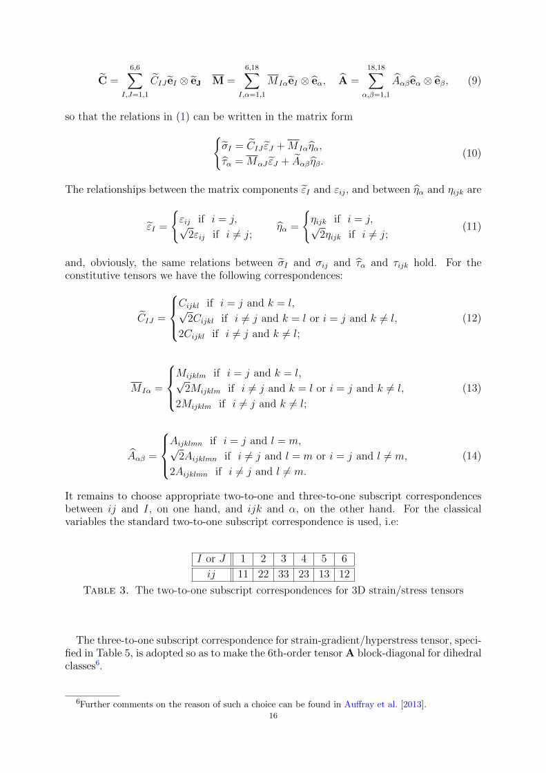
To obtain the normal forms for the different classes the generators provided in thefollowing table have been used :

Group GeneratorsZ−2 Pe3

Zn R(e3;

2πn

)Dn R

(e3;

2πn

), R(e1; π)

Z−2n, n ≥ 2 R(e3;

π

n

)·Pe3

Dh2n n ≥ 2 R

(e3;

π

n

)·Pe3 , R(e1, π)

Dvn R

(e3;

2π

n

), Pe1

T R(e3; π), R(e1; π), R(e1 + e2 + e3;2π

3)

O R(e3;π

2), R(e1; π), R(e1 + e2 + e3;

2π

3)

O− R(e3; π) ·Pe3 , Pe2+e3

Table 2. The set of group generators used to construct matrix represen-tation for each symmetry class.

The choice of the generators indicated in (2) has been made in order to have thefollowing relation:

M = Fix(D2)⊕ Fix(Dv2)⊕ Fix(Z−2 )

This relation means that any triclinic tensors M is the sum of three tensors M of highersymmetry. The consequence of this decomposition is used in the following to provideresults in a condensed form.

4.2. Orthonormal basis and matrix component ordering. Let be defined the fol-lowing spaces:

T(ij) = T ∈ ⊗2(R3)|T(ij) ; T(ij)k = T ∈ ⊗3(R3)|T(ij)kwhich are, in 3D, respectively, 6- and 18-dimensional vector spaces. Therefore

• the fourth-order elasticity tensor C is a self-adjoint endomorphism of T(ij);• the fifth-order coupling elasticity tensor M is a linear application from T(ij)k toT(ij);• the sixth-order elasticity tensor A is a self-adjoint endomorphism of T(ij)k.

In order to express the Cauchy-stress tensor σ, the strain tensor ε, the strain-gradienttensor η and the hyperstress tensor τ as 6- and 18-dimensional vectors and write C, Mand A as, respectively: a 6× 6, 6× 18 and 18× 18 matrices, we introduce the followingorthonormal basis vectors:

eI =

(1− δij√

2+δij2

)(ei ⊗ ej + ej ⊗ ei) , 1 ≤ I ≤ 6,

eα =

(1− δij√

2+δij2

)(ei ⊗ ej + ej ⊗ ei)⊗ ek, 1 ≤ α ≤ 18,

where the summation convention for a repeated subscript does not apply. Then, theaforementioned tensors can be expressed as:

ε =6∑I=1

εI eI , σ =6∑I=1

σI eI , η =18∑α=1

ηαeα, τ =18∑α=1

ταeα (8)

15

C =

6,6∑I,J=1,1

CIJ eI ⊗ eJ M =

6,18∑I,α=1,1

M IαeI ⊗ eα, A =

18,18∑α,β=1,1

Aαβeα ⊗ eβ, (9)

so that the relations in (1) can be written in the matrix formσI = CIJ εJ +M Iαηα,

τα = MαJ εJ + Aαβ ηβ.(10)

The relationships between the matrix components εI and εij, and between ηα and ηijk are

εI =

εij if i = j,√

2εij if i 6= j;ηα =

ηijk if i = j,√

2ηijk if i 6= j;(11)

and, obviously, the same relations between σI and σij and τα and τijk hold. For theconstitutive tensors we have the following correspondences:

CIJ =

Cijkl if i = j and k = l,√

2Cijkl if i 6= j and k = l or i = j and k 6= l,

2Cijkl if i 6= j and k 6= l;

(12)

M Iα =

Mijklm if i = j and k = l,√

2Mijklm if i 6= j and k = l or i = j and k 6= l,

2Mijklm if i 6= j and k 6= l;

(13)

Aαβ =

Aijklmn if i = j and l = m,√

2Aijklmn if i 6= j and l = m or i = j and l 6= m,

2Aijklmn if i 6= j and l 6= m.

(14)

It remains to choose appropriate two-to-one and three-to-one subscript correspondencesbetween ij and I, on one hand, and ijk and α, on the other hand. For the classicalvariables the standard two-to-one subscript correspondence is used, i.e:

I or J 1 2 3 4 5 6

ij 11 22 33 23 13 12

Table 3. The two-to-one subscript correspondences for 3D strain/stress tensors

The three-to-one subscript correspondence for strain-gradient/hyperstress tensor, speci-fied in Table 5, is adopted so as to make the 6th-order tensor A block-diagonal for dihedralclasses6.

6Further comments on the reason of such a choice can be found in Auffray et al. [2013].16

α or β 1 2 3 4 5 Type of mechanism

ijk 111 221 122 331 133 X-Interaction

α or β 6 7 8 9 10ijk 222 112 121 332 233 Y-Interaction

α or β 11 12 13 14 15ijk 333 113 131 223 232 Z-Interaction

α 16 17 18ijk 231 132 123 Coupling

Table 4. The three-to-one subscript correspondences for 3D strain-gradient/hyperstress tensors

The matrix representations of first- and second-order elasticity tensors have alreadybeen investigated. Hence, in the remaining subsection, attention will be limited to thetensor M.

4.3. Transformation matrix. Using the introduced orthogonal bases and the subscriptcorrespondences, the action of an orthogonal tensor Q ∈ O(3) on M can be represented

by two different matrices: a 6× 6 matrix Q, and a 18× 18 matrix Q in a way such that

QioQjpQkqQlrQmsMopqrs = QIJMJαQαβ (15)

where

QIJ =1

2(QioQjp +QipQjo) ; Qαβ =

1

2(QioQjp +QipQjo)Qkq (16)

with I and J being associated to ij and op, and α and β being associated to ijk and opqrespectively. Thus, formula (4) expressing the invariance of M under the action of Q isequivalent to

QMQT = M (17)

where M stands for the 6× 18 matrix of components MJα.The matrices provided hereafter are obtained by solving the linear system (17) for the

generators associated to the symmetry classes previously identified (c.f. Theorem 3.5).

4.4. Matrix representations for all symmetry classes.

4.4.1. Class symmetry characterized by 1. In this case, the material in question is totallyanisotropic and the SGE matrix M comprises 108 independent components. The explicitexpression of M as a full 6× 18 matrix is

MI =

A(15) B(15) C(15) D(9)

E(5) F (5) G(5) H(3)

I(5) J(5) K(5) L(3)

M(5) N(5) O(5) P (3)

To lighten the notations, in the following, the overline will be abandoned. The elementarymatrices are generic elements of the following spaces:

• A(15), B(15), C(15) ∈M(3, 5) ;• D(9) ∈M(3) ;• E(5), F (5), G(5), I(5), J (5), K(5), L(5), M (5), N (5), O(5) ∈M(1, 5) ;• H(3), L(3), P (3) ∈M(1, 3).

17

4.4.2. Symmetry classes [Zn], [Dn], [Dvn]. Classes [Dn] are chiral, classes [Dv

n] are polarwhile classes [Zn] has these two features. This fact is reflected, with the chosen generators,by the relation :

Fix(Zn) = Fix(Dn)⊕ Fix(Dvn) (18)

So only the matrices of MDn and MDvn

will be detailed, the remaining one being deducedfrom the above relation.Symmetry classes [Z2], [D2], [D

v2].

MD2 =

0 0 0 D(9)

E(5) 0 0 0

0 J(5) 0 0

0 0 O(5) 0

, MDv2

=

0 0 C(15) 0

0 F (5) 0 0

I(5) 0 0 0

0 0 0 P (3)

MZ2 = MD2 + MDv

2

It should be emphasized that these matrices are specific to the particular choice of sym-metry elements (generators) specified in Table 2. A different choice of generators willchange the location of the non-zero components.

Remark 4.2. It appears clearly that matrices MD2 and MDv2

can be made block diagonaland block anti-diagonal by choosing a three-to-one subscript correspondence that differsfrom the one indicated in Table 4. But doing so the well-structured shape of matricesrepresenting the sixth-order elasticity tensor A is lost [Auffray et al., 2013]. In the presentpaper, and in order to easily combining the new results with those already obtained inAuffray et al. [2013] we choose to keep the convention defined and used in this formerpublication. An alternative subscript correspondence can be used but, in this case, thematrices provided in Auffray et al. [2013] have to be permuted to be consistent.

Symmetry classes [Z3], [D3], [Dv3].

MD3 =

A(6) 0 0 D(4)

E(4) 0 0 H(2)

0 −E(4) 0 0

0 0 0 0

+

0 0 0 0

0 0 0 0

0 0 f(H(2)) 0

0 f(A(6)) f(D(4)) 0

MDv3

=

0 B(6) C(8) 0

0 F (4) 0 0

F (4) 0 0 L(2)

0 0 0 0

+

0 0 0 0

0 0 −f(L(2)) 0

0 0 0 0

−f(B(6)) 0 0 f(C(8))

MZ3 = MD3 + MDv

3

Symmetry classes [Z4], [D4], [Dv4].

MD4 =

0 0 0 D(4)

E(5) 0 0 0

0 −E(5) 0 0

0 0 O(2) 0

, MDv4

=

0 0 C(8) 0

0 F (5) 0 0

F (5) 0 0 0

0 0 0 P (2)

MZ4 = MD4 + MDv

4

18

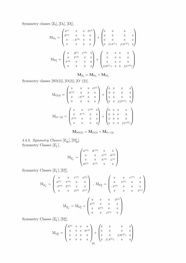
Symmetry classes [Z5], [D5], [Dv5].

MD5 =

A(1) 0 0 D(4)

E(4) 0 0 0

0 −E(4) 0 0

0 0 0 0

+

0 0 0

0 0 0 0

0 0 0 0

0 f(A(1)) f(D(4)) 0

MDv5

=

0 B(1) C(8) 0

0 F (4) 0 0

F (4) 0 0 0

0 0 0 0

+

0 0 0 0

0 0 0 0

0 0 0 0

f(B(1)) 0 0 f(C(8))

MZ5 = MD5 + MDv

5

Symmetry classes [SO(2)], [O(2)], [O−(2)].

MO(2) =

0 0 0 D(4)

E(4) 0 0 0

0 −E(4) 0 0

0 0 0 0

+

0 0 0 0

0 0 0 0

0 0 0 0

0 0 f(D(4)) 0

MO−(2) =

0 0 C(8) 0

0 F (4) 0 0

F (4) 0 0 0

0 0 0 0

+

0 0 0 0

0 0 0 0

0 0 0 0

0 0 0 f(C(8))

MSO(2) = MO(2) + MO−(2)

4.4.3. Symmetry Classes [Z−2p], [Dh2p].

Symmetry Classes [Z−2 ].

MZ−2=

A(15) B(15) 0 0

0 0 G(5) H(3)

0 0 K(5) L(3)

M(5) N(5) 0 0

Symmetry Classes [Z−4 ], [Dh

4 ].

MZ−4=

0 0 C(7) D(5)

E(5) F (5) 0 0

−F (5) E(5) 0 0

0 0 O(3) P (1)

, MDh4

=

0 0 C(7) 0

0 F (5) 0 0

−F (5) 0 0 0

0 0 0 P (1)

MZ−4= MDh

4+

0 0 0 D(5)

E(5) 0 0 0

0 E(5) 0 0

0 0 O(3) 0

Symmetry Classes [Z−6 ], [Dh

6 ].

MDh6

=

A(6) 0 0 0

0 0 0 H(2)

0 0 0 0

0 0 0 0

+

0 0 0 0

0 0 0 0

0 0 f(H(2)) 0

0 f(A(6)) 0 0

19

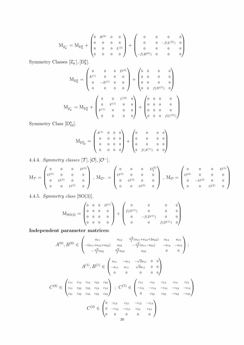
MZ−6= MDh

6+

0 B(6) 0 0

0 0 0 0

0 0 0 L(2)

0 0 0 0

+

0 0 0 0

0 0 −f(L(2)) 0

0 0 0 0

−f(B(6)) 0 0 0

Symmetry Classes [Z−8 ], [Dh

8 ].

MDh8

=

0 0 0 D(2)

E(1) 0 0 0

0 −E(1) 0 0

0 0 0 0

+

0 0 0 0

0 0 0 0

0 0 0 0

0 0 f(D(2)) 0

MZ−8= MDh

8+

0 0 C(2) 0

0 F (1) 0 0

F (1) 0 0 0

0 0 0 0

+

0 0 0 0

0 0 0 0

0 0 0 0

0 0 0 f(C(2))

Symmetry Class [Dh

10].

MDh10

=

A(1) 0 0 0

0 0 0 0

0 0 0 0

0 0 0 0

+

0 0 0 0

0 0 0 0

0 0 0 0

0 f(A(1)) 0 0

4.4.4. Symmetry classes [T ], [O], [O−].

MT =

0 0 0 D(3)

O(5) 0 0 0

0 O(5) 0 0

0 0 O(5) 0

, MO− =

0 0 0 D

(2)2

O(3) 0 0 0

0 O(3) 0 0

0 0 O(3) 0

, MO =

0 0 0 D(1)

O(2) 0 0 0

0 −O(2) 0 0

0 0 O(2) 0

4.4.5. Symmetry class [SO(3)].

MSO(3) =

0 0 0 D(1)

0 0 0 0

0 0 0 0

0 0 0 0

+

0 0 0 0

f(D(1)) 0 0 0

0 −f(D(1)) 0 0

0 0 f(D(1)) 0

Independent parameter matrices:

A(6), B(6) ∈

a11 a12√2

2(a11+a12+2a22) a14 a15

−(a11+a12+a22) a22 −√

22(a11−a22) −a14 −a15

−√

22a33

√2

2a33 a33 0 0

;

A(1), B(1) ∈

a11 −a11 −√2a11 0 0

−a11 a11√2a11 0 0

0 0 0 0 0

C(8) ∈

c11 c12 c13 c22 c23

c11 c22 c23 c12 c13

c31 c32 c33 c32 c33

; C(7) ∈

c11 c12 c13 c14 c15

−c11 −c14 −c15 −c12 −c130 c32 c33 −c32 −c33

C(2) ∈

0 c12 c13 −c12 −c130 −c12 −c13 c12 c13

0 0 0 0 0

20

D(5) ∈

d11 d12 d13

d12 d11 d13

d31 d31 d33

; D(4) ∈

d11 d12 d13

−d12 −d11 −d13d31 −d31 0

; D(3) ∈

d11 d12 d13

d13 d11 d12

d12 d13 d11

D(2) ∈

d11 d11 d13

−d11 −d11 −d130 0 0

; D(2)2 ∈

d11 d12 d12

d12 d11 d12

d12 d12 d11

; D(1) ∈

0 d12 −d12−d12 0 d12

d12 −d12 0

E(4), F (4) ∈

(e11 e12

√2

2(e11−e12) e14 e15

); E(1), F (1) ∈

(e11 −e11 −

√2e11 0 0

)H(2), L(2), P (2) ∈

(h11 h11 h13

)O(3) ∈

(o11 o12 o13 o12 o13

); O(2) ∈

(0 o12 o13 −o12 −o13

)Non-independent parameter matrices:

f(A(6)), f(B(6)) =(−√22(2a11+a12+a22) −

√2

2(a12−a22) −(a11+a22) −

√2a14 −

√2a15

)f(A(1)), f(B(1)) ∈

(√2a11 −

√2a11 2a11 0 0

)f(C(2)) ∈

(−√2c13 −

√2c13 −2c12

)f(C(8)) =

(√2

2(c13−c23)

√2

2(c13−c23) c12−c22

)f(D(2)) ∈

(0 d13

√2d11 −d13 −

√2d11

)f(D(4)) =

(0 −d13 −

√2

2(d11+d12) d13

√22(d11+d12)

)f(D(1)) ∈

(0 d12 −

√22d12 −d12

√2

2d12

)f(H(2)), f(L(2)) =

(0 −

√2

2h13 −h12

√2

2h13 h12

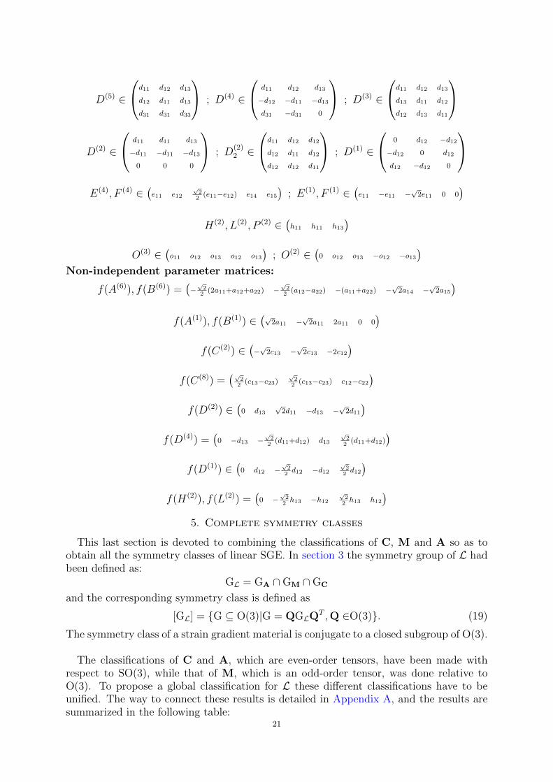
)5. Complete symmetry classes

This last section is devoted to combining the classifications of C, M and A so as toobtain all the symmetry classes of linear SGE. In section 3 the symmetry group of L hadbeen defined as:

GL = GA ∩GM ∩GC

and the corresponding symmetry class is defined as

[GL] = G ⊆ O(3)|G = QGLQT ,Q ∈O(3). (19)

The symmetry class of a strain gradient material is conjugate to a closed subgroup of O(3).

The classifications of C and A, which are even-order tensors, have been made withrespect to SO(3), while that of M, which is an odd-order tensor, was done relative toO(3). To propose a global classification for L these different classifications have to beunified. The way to connect these results is detailed in Appendix A, and the results aresummarized in the following table:

21

Symmetry class for the constitutive law Symmetry class for the even-order tensors[Zn] [Zn ⊕ Zc2][Dn] [Dn ⊕ Zc2][Zc2] [Z2 ⊕ Zc2][Z−2 ] [Z2 ⊕ Zc2][Z−2n] [Z2n ⊕ Zc2]

[Dh2n] [D2n ⊕ Zc2]

[Dvn] [Dn ⊕ Zc2]

[O(2)−] [O(2)⊕ Zc]2

[O−] [O ⊕ Zc2][P ] [P ⊕ Zc2]

Table 5. How a symmetry group in O(3) is viewed by an even-order tensor.In this table P stands for a exceptional group.

As a result, the 3D strain-gradient elasticity is divided into 48 symmetry classes7. Thenature of these classes and the associated number of independent parameters are providedin the two following tables:

Name Triclinic Monoclinic Orthotropic Trigonal Tetragonal Pentagonal Hexagonal ∞-gonal

[GL] 1 [Z2] [Z3] [Z4] [Z5] [Z6] [SO(2)]#indep(L) 300 156 99 77 62 58 56

[GL] [D2] [D3] [D4] [D5] [D6] [O(2)]

#indep(L) 84 56 45 37 35 34

[GL] [Zc2] [Z2 ⊕ Zc2] [Z3 ⊕ Zc2] [Z4 ⊕ Zc2] [Z5 ⊕ Zc2] [Z6 ⊕ Zc2] [SO(2)⊕ Zc2]#indep(L) 192 104 63 51 40 38 36

[GL] [D2 ⊕ Zc2] [D3 ⊕ Zc2] [D4 ⊕ Zc2] [D5 ⊕ Zc2] [D6 ⊕ Zc2] [O(2)⊕ Zc2]#indep(L) 60 40 34 28 27 26

[GL] [Z−2 ] [Z−4 ] [Z−6 ] [Z−8 ]#indep(L) 160 77 54 42

[GL] [Dv2] [Dv

3] [Dv4] [Dv

5] [O−(2)]#indep(L) 88 60 49 41 38

[GL] [Dh4 ] [Dh

6 ] [Dh8 ] [Dh

10]#indep(L) 47 35 29 27

Table 6. The names, the sets of subgroups [GL] and the numbers of inde-pendent components #indep(L) for the plane symmetry classes of SGE.

7This result is found through inspection by combining the results of our classification. More precisely,for each possible material symmetry class, we determine the least symmetric triplet of physical symmetryclasses compatible with the material symmetries.

22

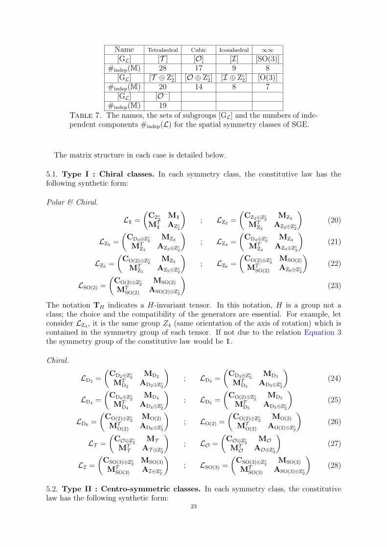
Name Tetrahedral Cubic Icosahedral ∞∞[GL] [T ] [O] [I] [SO(3)]

#indep(M) 28 17 9 8[GL] [T ⊕ Zc2] [O ⊕ Zc2] [I ⊕ Zc2] [O(3)]

#indep(M) 20 14 8 7[GL] [O−]

#indep(M) 19

Table 7. The names, the sets of subgroups [GL] and the numbers of inde-pendent components #indep(L) for the spatial symmetry classes of SGE.

The matrix structure in each case is detailed below.

5.1. Type I : Chiral classes. In each symmetry class, the constitutive law has thefollowing synthetic form:

Polar & Chiral.

L1 =

(CZc

2M1

MT1 AZc

2

); LZ2 =

(CZ2⊕Zc

2MZ2

MTZ2

AZ2⊕Zc2

)(20)

LZ3 =

(CD3⊕Zc

2MZ3

MTZ3

AZ3⊕Zc2

); LZ4 =

(CD4⊕Zc

2MZ4

MTZ4

AZ4⊕Zc2

)(21)

LZ5 =

(CO(2)⊕Zc

2MZ5

MTZ5

AZ5⊕Zc2

); LZ6 =

(CO(2)⊕Zc

2MSO(2)

MTSO(2) AZ6⊕Zc

2

)(22)

LSO(2) =

(CO(2)⊕Zc

2MSO(2)

MTSO(2) ASO(2)⊕Zc

2

)(23)

The notation TH indicates a H-invariant tensor. In this notation, H is a group not aclass; the choice and the compatibility of the generators are essential. For example, letconsider LZ4 , it is the same group Z4 (same orientation of the axis of rotation) which iscontained in the symmetry group of each tensor. If not due to the relation Equation 3the symmetry group of the constitutive law would be 1.

Chiral.

LD2 =

(CD2⊕Zc

2MD2

MTD2

AD2⊕Zc2

); LD3 =

(CD3⊕Zc

2MD3

MTD3

AD3⊕Zc2

)(24)

LD4 =

(CD4⊕Zc

2MD4

MTD4

AD4⊕Zc2

); LD5 =

(CO(2)⊕Zc

2MD5

MTD5

AD5⊕Zc2

)(25)

LD6 =

(CO(2)⊕Zc

2MO(2)

MTO(2) AD6⊕Zc

2

); LO(2) =

(CO(2)⊕Zc

2MO(2)

MTO(2) AO(2)⊕Zc

2

)(26)

LT =

(CO⊕Zc

2MT

MTT AT ⊕Zc

2

); LO =

(CO⊕Zc

2MO

MTO AO⊕Zc

2

)(27)

LI =

(CSO(3)⊕Zc

2MSO(3)

MTSO(3) AI⊕Zc

2

); LSO(3) =

(CSO(3)⊕Zc

2MSO(3)

MTSO(3) ASO(3)⊕Zc

2

)(28)

5.2. Type II : Centro-symmetric classes. In each symmetry class, the constitutivelaw has the following synthetic form:

23

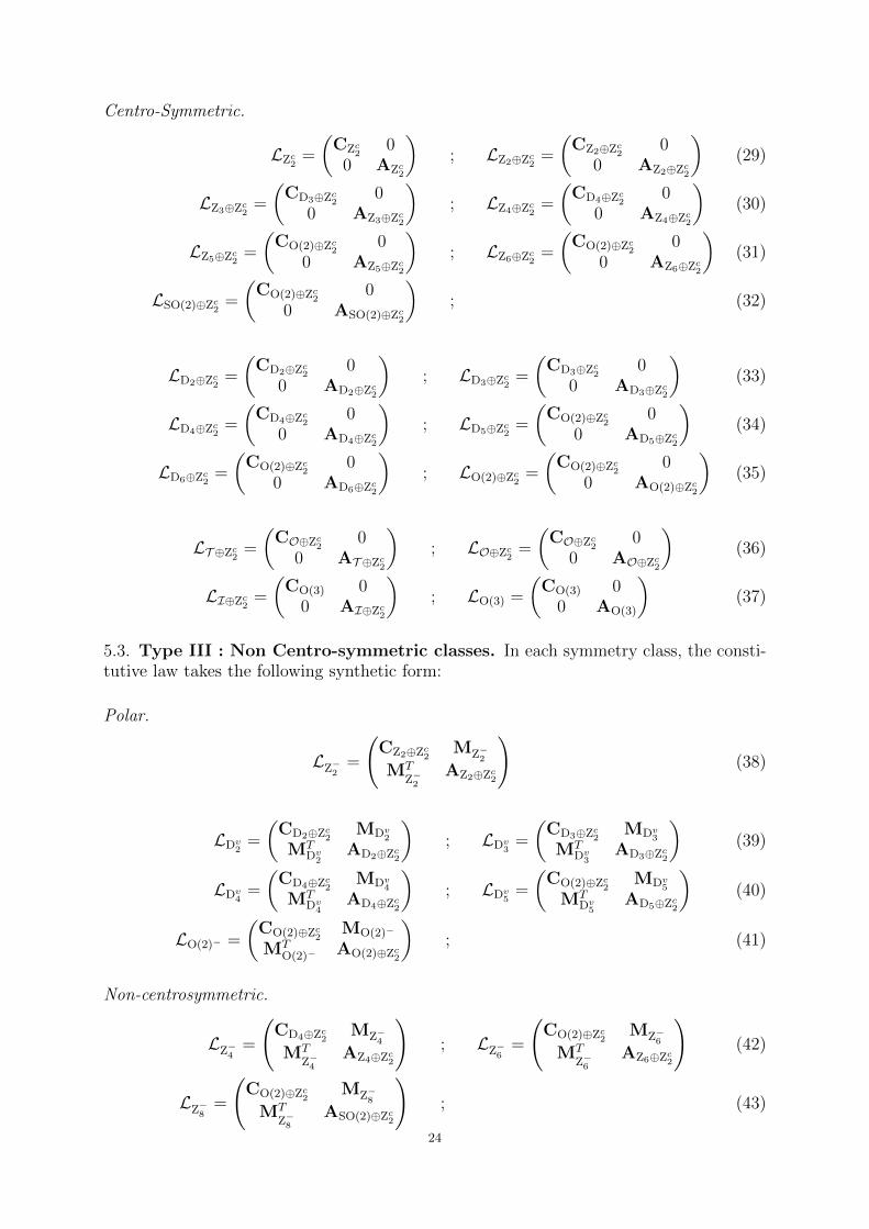
Centro-Symmetric.

LZc2

=

(CZc

20

0 AZc2

); LZ2⊕Zc

2=

(CZ2⊕Zc

20

0 AZ2⊕Zc2

)(29)

LZ3⊕Zc2

=

(CD3⊕Zc

20

0 AZ3⊕Zc2

); LZ4⊕Zc

2=

(CD4⊕Zc

20

0 AZ4⊕Zc2

)(30)

LZ5⊕Zc2

=

(CO(2)⊕Zc

20

0 AZ5⊕Zc2

); LZ6⊕Zc

2=

(CO(2)⊕Zc

20

0 AZ6⊕Zc2

)(31)

LSO(2)⊕Zc2

=

(CO(2)⊕Zc

20

0 ASO(2)⊕Zc2

); (32)

LD2⊕Zc2

=

(CD2⊕Zc

20

0 AD2⊕Zc2

); LD3⊕Zc

2=

(CD3⊕Zc

20

0 AD3⊕Zc2

)(33)

LD4⊕Zc2

=

(CD4⊕Zc

20

0 AD4⊕Zc2

); LD5⊕Zc

2=

(CO(2)⊕Zc

20

0 AD5⊕Zc2

)(34)

LD6⊕Zc2

=

(CO(2)⊕Zc

20

0 AD6⊕Zc2

); LO(2)⊕Zc

2=

(CO(2)⊕Zc

20

0 AO(2)⊕Zc2

)(35)

LT ⊕Zc2

=

(CO⊕Zc

20

0 AT ⊕Zc2

); LO⊕Zc

2=

(CO⊕Zc

20

0 AO⊕Zc2

)(36)

LI⊕Zc2

=

(CO(3) 0

0 AI⊕Zc2

); LO(3) =

(CO(3) 0

0 AO(3)

)(37)

5.3. Type III : Non Centro-symmetric classes. In each symmetry class, the consti-tutive law takes the following synthetic form:

Polar.

LZ−2=

(CZ2⊕Zc

2MZ−2

MTZ−2

AZ2⊕Zc2

)(38)

LDv2

=

(CD2⊕Zc

2MDv

2

MTDv

2AD2⊕Zc

2

); LDv

3=

(CD3⊕Zc

2MDv

3

MTDv

3AD3⊕Zc

2

)(39)

LDv4

=

(CD4⊕Zc

2MDv

4

MTDv

4AD4⊕Zc

2

); LDv

5=

(CO(2)⊕Zc

2MDv

5

MTDv

5AD5⊕Zc

2

)(40)

LO(2)− =

(CO(2)⊕Zc

2MO(2)−

MTO(2)− AO(2)⊕Zc

2

); (41)

Non-centrosymmetric.

LZ−4=

(CD4⊕Zc

2MZ−4

MTZ−4

AZ4⊕Zc2

); LZ−6

=

(CO(2)⊕Zc

2MZ−6

MTZ−6

AZ6⊕Zc2

)(42)

LZ−8=

(CO(2)⊕Zc

2MZ−8

MTZ−8

ASO(2)⊕Zc2

); (43)

24

LDh4

=

(CD4⊕Zc

2MDh

4

MTDh

4AD4⊕Zc

2

); LDh

6=

(CO(2)⊕Zc

2MDh

6

MTDh

6AD6⊕Zc

2

)(44)

LDh8

=

(CO(2)⊕Zc

2MDh

8

MTDh

8AO(2)⊕Zc

2

); LDh

10=

(CO(2)⊕Zc

2MDh

10

MTDh

10AO(2)⊕Zc

2

)(45)

LO− =

(CO⊕Zc

2MO−

MTO− AO⊕Zc

2

)(46)

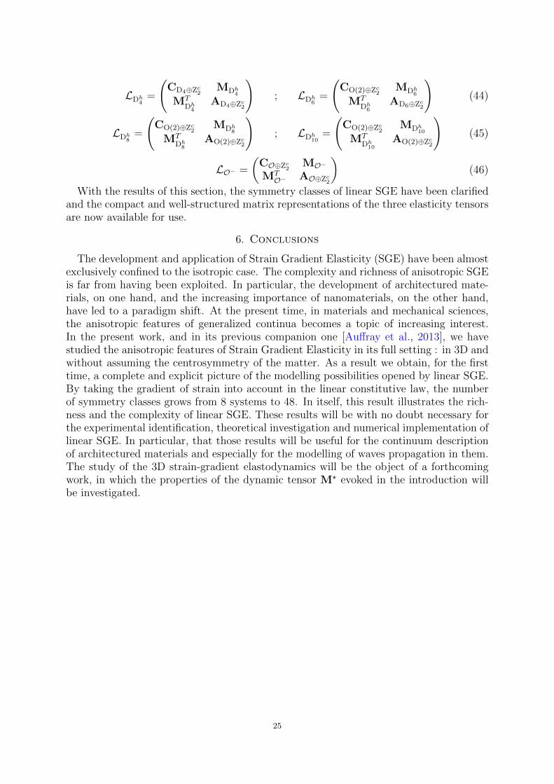
With the results of this section, the symmetry classes of linear SGE have been clarifiedand the compact and well-structured matrix representations of the three elasticity tensorsare now available for use.

6. Conclusions

The development and application of Strain Gradient Elasticity (SGE) have been almostexclusively confined to the isotropic case. The complexity and richness of anisotropic SGEis far from having been exploited. In particular, the development of architectured mate-rials, on one hand, and the increasing importance of nanomaterials, on the other hand,have led to a paradigm shift. At the present time, in materials and mechanical sciences,the anisotropic features of generalized continua becomes a topic of increasing interest.In the present work, and in its previous companion one [Auffray et al., 2013], we havestudied the anisotropic features of Strain Gradient Elasticity in its full setting : in 3D andwithout assuming the centrosymmetry of the matter. As a result we obtain, for the firsttime, a complete and explicit picture of the modelling possibilities opened by linear SGE.By taking the gradient of strain into account in the linear constitutive law, the numberof symmetry classes grows from 8 systems to 48. In itself, this result illustrates the rich-ness and the complexity of linear SGE. These results will be with no doubt necessary forthe experimental identification, theoretical investigation and numerical implementation oflinear SGE. In particular, that those results will be useful for the continuum descriptionof architectured materials and especially for the modelling of waves propagation in them.The study of the 3D strain-gradient elastodynamics will be the object of a forthcomingwork, in which the properties of the dynamic tensor M? evoked in the introduction willbe investigated.

25

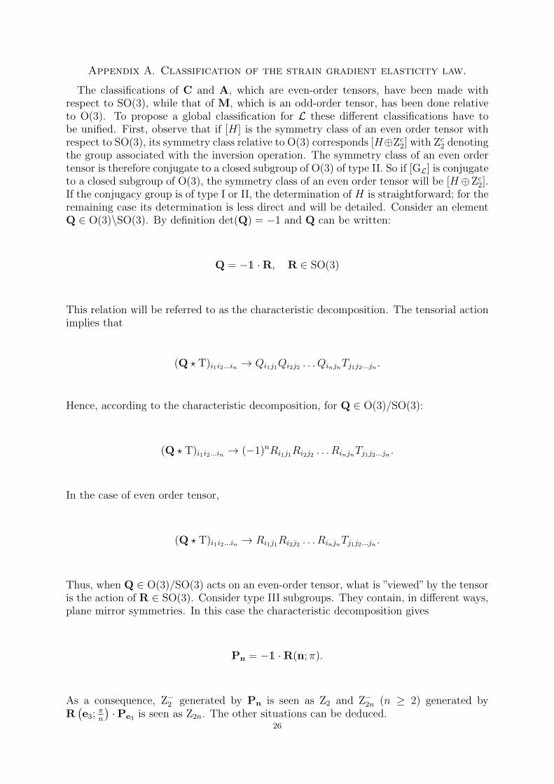
Appendix A. Classification of the strain gradient elasticity law.

The classifications of C and A, which are even-order tensors, have been made withrespect to SO(3), while that of M, which is an odd-order tensor, has been done relativeto O(3). To propose a global classification for L these different classifications have tobe unified. First, observe that if [H] is the symmetry class of an even order tensor withrespect to SO(3), its symmetry class relative to O(3) corresponds [H⊕Zc2] with Zc2 denotingthe group associated with the inversion operation. The symmetry class of an even ordertensor is therefore conjugate to a closed subgroup of O(3) of type II. So if [GL] is conjugateto a closed subgroup of O(3), the symmetry class of an even order tensor will be [H⊕Zc2].If the conjugacy group is of type I or II, the determination of H is straightforward; for theremaining case its determination is less direct and will be detailed. Consider an elementQ ∈ O(3)\SO(3). By definition det(Q) = −1 and Q can be written:

Q = −1 ·R, R ∈ SO(3)

This relation will be referred to as the characteristic decomposition. The tensorial actionimplies that

(Q ? T)i1i2...in → Qi1j1Qi2j2 . . . QinjnTj1j2...jn .

Hence, according to the characteristic decomposition, for Q ∈ O(3)/SO(3):

(Q ? T)i1i2...in → (−1)nRi1j1Ri2j2 . . . RinjnTj1j2...jn .

In the case of even order tensor,

(Q ? T)i1i2...in → Ri1j1Ri2j2 . . . RinjnTj1j2...jn .

Thus, when Q ∈ O(3)/SO(3) acts on an even-order tensor, what is ”viewed” by the tensoris the action of R ∈ SO(3). Consider type III subgroups. They contain, in different ways,plane mirror symmetries. In this case the characteristic decomposition gives

Pn = −1 ·R(n; π).

As a consequence, Z−2 generated by Pn is seen as Z2 and Z−2n (n ≥ 2) generated byR(e3;

πn

)·Pe3 is seen as Z2n. The other situations can be deduced.

26

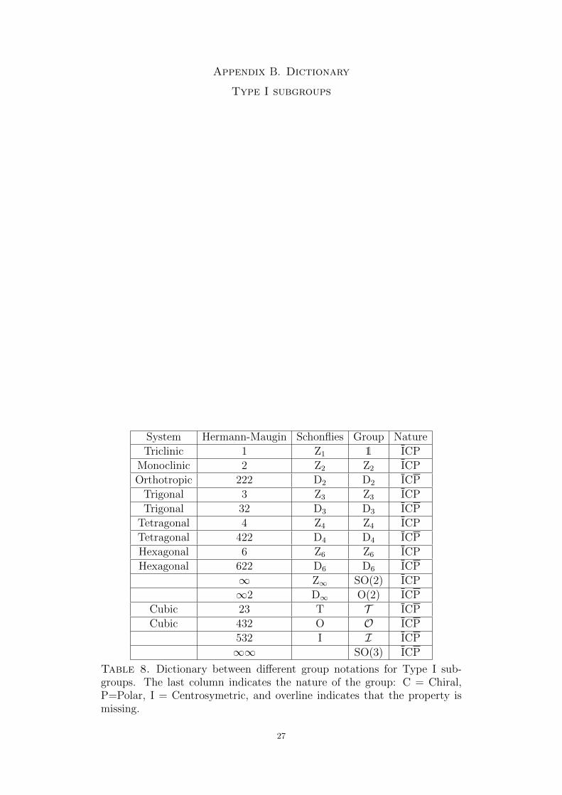
Appendix B. Dictionary

Type I subgroups

System Hermann-Maugin Schonflies Group Nature

Triclinic 1 Z1 1 ICP

Monoclinic 2 Z2 Z2 ICP

Orthotropic 222 D2 D2 ICP

Trigonal 3 Z3 Z3 ICP

Trigonal 32 D3 D3 ICP

Tetragonal 4 Z4 Z4 ICP

Tetragonal 422 D4 D4 ICP

Hexagonal 6 Z6 Z6 ICP

Hexagonal 622 D6 D6 ICP

∞ Z∞ SO(2) ICP

∞2 D∞ O(2) ICP

Cubic 23 T T ICP

Cubic 432 O O ICP

532 I I ICP

∞∞ SO(3) ICP

Table 8. Dictionary between different group notations for Type I sub-groups. The last column indicates the nature of the group: C = Chiral,P=Polar, I = Centrosymetric, and overline indicates that the property ismissing.

27

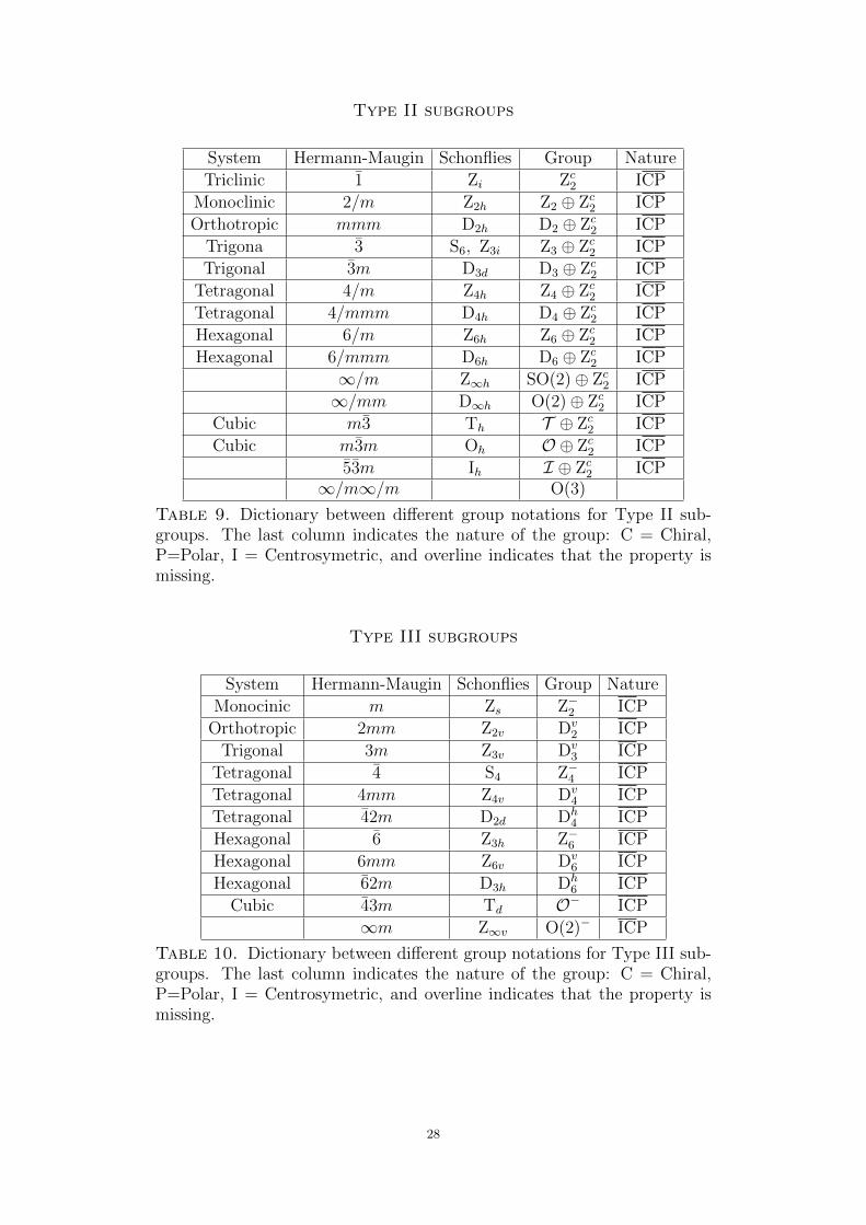
Type II subgroups

System Hermann-Maugin Schonflies Group Nature

Triclinic 1 Zi Zc2 ICP

Monoclinic 2/m Z2h Z2 ⊕ Zc2 ICP

Orthotropic mmm D2h D2 ⊕ Zc2 ICP

Trigona 3 S6, Z3i Z3 ⊕ Zc2 ICP

Trigonal 3m D3d D3 ⊕ Zc2 ICP

Tetragonal 4/m Z4h Z4 ⊕ Zc2 ICP

Tetragonal 4/mmm D4h D4 ⊕ Zc2 ICP

Hexagonal 6/m Z6h Z6 ⊕ Zc2 ICP

Hexagonal 6/mmm D6h D6 ⊕ Zc2 ICP

∞/m Z∞h SO(2)⊕ Zc2 ICP

∞/mm D∞h O(2)⊕ Zc2 ICP

Cubic m3 Th T ⊕ Zc2 ICP

Cubic m3m Oh O ⊕ Zc2 ICP

53m Ih I ⊕ Zc2 ICP∞/m∞/m O(3)

Table 9. Dictionary between different group notations for Type II sub-groups. The last column indicates the nature of the group: C = Chiral,P=Polar, I = Centrosymetric, and overline indicates that the property ismissing.

Type III subgroups

System Hermann-Maugin Schonflies Group Nature

Monocinic m Zs Z−2 ICP

Orthotropic 2mm Z2v Dv2 ICP

Trigonal 3m Z3v Dv3 ICP

Tetragonal 4 S4 Z−4 ICP

Tetragonal 4mm Z4v Dv4 ICP

Tetragonal 42m D2d Dh4 ICP

Hexagonal 6 Z3h Z−6 ICP

Hexagonal 6mm Z6v Dv6 ICP

Hexagonal 62m D3h Dh6 ICP

Cubic 43m Td O− ICP

∞m Z∞v O(2)− ICP

Table 10. Dictionary between different group notations for Type III sub-groups. The last column indicates the nature of the group: C = Chiral,P=Polar, I = Centrosymetric, and overline indicates that the property ismissing.

28

References

N.C. Admal, J. Marian, and G. Po. The atomistic representation of first strain-gradientelastic tensors. Journal of the Mechanics and Physics of Solids, 99:93–115, 2017.

J.-J. Alibert, P. Seppecher, and F. dell’Isola. Truss modular beams with deformationenergy depending on higher displacement gradients. Mathematics and Mechanics ofSolids, 8(1):51–73, 2003.

N. Auffray. On the algebraical structure of isotropic generalized elasticity theories. Math-ematics and Mechanics of Solids, page 1081286513507941, 2013.

N. Auffray. Analytical expressions for odd-order anisotropic tensor dimension. ComptesRendus Mecanique, 342(5):284–291, 2014.

N. Auffray, R. Bouchet, and Y. Brechet. Derivation of anisotropic matrix for bi-dimensional strain-gradient elasticity behavior. International Journal of Solids andStructures, 46(2):440–454, 2009.

N. Auffray, H. Le Quang, and Q.C. He. Matrix representations for 3D strain-gradientelasticity. Journal of the Mechanics and Physics of Solids, 61(5):1202–1223, 2013.

N. Auffray, J. Dirrenberger, and G. Rosi. A complete description of bi-dimensionalanisotropic strain-gradient elasticity. International Journal of Solids and Structures,69-70:195–206, 2015.

N. Auffray, B. Kolev, and M. Olive. Handbook of bidimensional tensors: Part i:Decomposition and symmetry classes. Mathematics and Mechanics of Solids, page1081286516649017, 2016.

A. Bacigalupo and L. Gambarotta. Homogenization of periodic hexa-and tetrachiral cel-lular solids. Composite Structures, 116:461–476, 2014a.

A. Bacigalupo and L. Gambarotta. Second-gradient homogenized model for wave propa-gation in heterogeneous periodic media. International Journal of Solids and Structures,51(5):1052–1065, 2014b.

A. Bacigalupo and L. Gambarotta. Wave propagation in non-centrosymmetric beam-lattices with lumped masses: Discrete and micropolar modeling. International Journalof Solids and Structures, 118:128–145, 2017.

A. Bertram. Compendium on gradient materials, 2016.J.-P. Boehler, A.A. Kirillov, Jr., and E.T. Onat. On the polynomial invariants of the

elasticity tensor. Journal of Elasticity, 34(2):97–110, 1994.C. Boutin. Microstructural effects in elastic composites. International Journal of Solids

and Structures, 33(7):1023–1051, 1996.Y. Brechet and J. D. Embury. Architectured materials: expanding materials space. Scripta

Materialia, 68(1):1–3, 2013.L. E. Cross. Flexoelectric effects: Charge separation in insulating solids subjected to

elastic strain gradients. Journal of Materials Science, 41(1):53–63, 2006.F. dell’Isola and D. Steigmann. A two-dimensional gradient-elasticity theory for woven

fabrics. Journal of Elasticity, 118(1):113–125, 2015.F. dell’Isola, G. Sciarra, and S. Vidoli. Generalized hooke’s law for isotropic second

gradient materials. Proceedings of the Royal Society London A, 465:2177–2196, 2009.F dell’Isola, I Giorgio, M. Pawlikowski, and N.L. Rizzi. Large deformations of planar

extensible beams and pantographic lattices: heuristic homogenization, experimentaland numerical examples of equilibrium. Proc. R. Soc. A, 472(2185):20150790, 2016.

S. Forte and M. Vianello. Symmetry classes for elasticity tensors. Journal of Elasticity.,43(2):81–108, 1996.

P. Germain. The method of virtual power in continuum mechanics. part 2: Microstructure.SIAM Journal on Applied Mathematics, 25(3):556–575, 1973.

29

Q.-C. He and Q.-S. Zheng. On the symmetries of 2D elastic and hyperelastic tensors.Journal of elasticity, 43:203–225, 1996.

D. Iesan. On the torsion of chiral bars in gradient elasticity. International Journal ofSolids and Structures, 50(3):588–594, 2013.

D. Iesan. Fundamental solutions for chiral solids in gradient elasticity. Mechanics ResearchCommunications, 61:47–52, 2014.

D. Iesan and R. Quintanilla. On chiral effects in strain gradient elasticity. EuropeanJournal of Mechanics-A/Solids, 58:233–246, 2016.

E. Ihrig and M. Golubitsky. Pattern selection with O(3) symmetry. Physica D. NonlinearPhenomena, 13(1-2):1–33, 1984.

R. Lakes. Elastic and viscoelastic behavior of chiral materials. International Journal ofMechanical Sciences, 43(7):1579–1589, 2001.

R. Lakes and R. Benedict. Noncentrosymmetry in micropolar elasticity. InternationalJournal of Engineering Science, 20(10):1161–1167, 1982.

M. Lazar and G. Po. The non-singular green tensor of mindlin’s anisotropic gradientelasticity with separable weak non-locality. Physics Letters A, 379(24-25):1538–1543,2015.

H. Le Quang and Q.-C. He. The number and types of all possible rotational symmetriesfor flexoelectric tensors. Proceedings of the Royal Society A, 467(2132):2369–2386, 2011.

X. N. Liu and G. K. Hu. Elastic metamaterials making use of chirality: a review. Strojniskivestnik-Journal of Mechanical Engineering, 62(7-8):403–418, 2016.

X. N. Liu, G. Huang, and G. K. Hu. Chiral effect in plane isotropic micropolar elasticityand its application to chiral lattices. Journal of the Mechanics and Physics of Solids,60(11):1907–1921, 2012.

A. E. H. Love. A treatise on the mathematical theory of elasticity. Cambridge universitypress, 1944.

R. Maranganti and P. Sharma. A novel atomistic approach to determine strain-gradientelasticity constants: Tabulation and comparison for various metals, semiconductors,silica, polymers and the (ir) relevance for nanotechnologies. Journal of the Mechanicsand Physics of Solids, 55(9):1823–1852, 2007.

G. Maugin. Generalized continuum mechanics: what do we mean by that? In Mechanicsof Generalized Continua, pages 3–13. Springer, 2010.

M. M. Mehrabadi and S.C. Cowin. Eigentensors of linear anisotropic elastic materials.The Quarterly Journal of Mechanics and Applied Mathematics, 43:15–41, 1990.

R.D. Mindlin. Micro-structure in linear elasticity. Archive for Rational Mechanics andAnalysis, 16(1), 1964.

R.D. Mindlin and N.N. Eshel. On first strain-gradient theories in linear elasticity. Inter-national Journal of Solids and Structures, 4(1):109–124, 1968.

S. M. Mousavi, J. N. Reddy, and J. Romanoff. Analysis of anisotropic gradient elasticshear deformable plates. Acta Mechanica, 227(12):3639–3656, 2016.

M. Olive and N. Auffray. Symmetry classes for even-order tensors. Mathematics andMechanics of Complex Systems, 1:177–210, 2013.

M. Olive and N. Auffray. Symmetry classes for odd-order tensors. ZAMM-Zeitschrift furAngewandte Mathematik und Mechanik, 94:421–447, 2014a.

M. Olive and N. Auffray. Isotropic invariants of completely symmetric third-order tensors.Journal of Mathematical Physic, 55:092901, 2014b.

M. Olive, B. Kolev, and N. Auffray. A minimal integrity basis for the elasticity tensor.Archive for Rational Mechanics and Analysis, 226(1):1–31, 2017.

S. A. Papanicolopulos. Chirality in isotropic linear gradient elasticity. InternationalJournal of Solids and Structures, 48(5):745–752, 2011.

30

L. Placidi, U. Andreaus, and I. Giorgio. Identification of two-dimensional pantographicstructure via a linear d4 orthotropic second gradient elastic model. Journal of Engi-neering Mathematics, pages 1–21, 2016.

C. Polizzotto. A hierarchy of simplified constitutive models within isotropic strain gradientelasticity. European Journal of Mechanics-A/Solids, 61:92–109, 2017.

C. Polizzotto. Anisotropy in strain gradient elasticity: Simplified models with differentforms of internal length and moduli tensors. European Journal of Mechanics-A/Solids,71:51–63, 2018.

M. Poncelet, A. Somera, C. Morel, C. Jailin, and N. Auffray. An experimental evidenceof the failure of Cauchy elasticity for the overall modeling of a non-centro-symmetriclattice under static loading. International Journal of Solids and Structures, 147:223–237, 2018.

D. L. Portigal and E. Burstein. Acoustical activity and other first-order spatial dispersioneffects in crystals. Physical Review, 170(3):673, 1968.

H. Reda, N. Karathanasopoulos, Y. Rahali, J.-F. Ganghoffer, and H. Lakiss. Influenceof first to second gradient coupling energy terms on the wave propagation of three-dimensional non-centrosymmetric architectured materials. International Journal ofEngineering Science, 128:151–164, 2018.

G. Rosi and N. Auffray. Anisotropic and dispersive wave propagation within strain-gradient framework. Wave Motion, 63:120–134, 2016.

S. Sternberg. Group theory and physics. Cambridge University Press, Cambridge, 1994.ISBN 0-521-24870-1.

R. A. Toupin. Elastic materials with couple-stresses. Archive for Rational Mechanics andAnalysis, 11:385–414, 1962.

C. Truesdell and W. Noll. The non-linear field theories of mechanics. In The non-linearfield theories of mechanics, pages 1–579. Springer, 1965.

C. Truesdell and R. Toupin. The classical field theories. In Principles of classical me-chanics and field theory, pages 226–858. Springer, 1960.

M. Vianello. An integrity basis for plane elasticity tensors. Archives of Mechanics, 49:197–208, 1997.

S. T. Yaghoubi, S. M. Mousavi, and J. Paavola. Size effects on centrosymmetric anisotropicshear deformable beam structures. ZAMM-Journal of Applied Mathematics and Me-chanics, 97(5):586–601, 2017.

J. Yvonnet and L.P. Liu. A numerical framework for modeling flexoelectricity and maxwellstress in soft dielectrics at finite strains. Computer Methods in Applied Mechanics andEngineering, 313:450–482, 2017.

Q.-S. Zheng and J.-P. Boehler. The description, classification, and reality of material andphysical symmetries. Acta Mechanica, 102(1-4):73–89, 1994.

P. Zubko, G. Catalan, and A. K. Tagantsev. Flexoelectric effect in solids. Annual Reviewof Materials Research, 43:387–421, 2013.

MSME, Universite Paris-Est, Laboratoire Modelisation et Simulation Multi Echelle,MSMEUMR 8208 CNRS, 5 bd Descartes, 77454 Marne-la-Vallee, France

E-mail address: Nicolas.auffray@univ-mlv.fr

MSME, Universite Paris-Est, Laboratoire Modelisation et Simulation Multi Echelle,MSMEUMR 8208 CNRS, 5 bd Descartes, 77454 Marne-la-Vallee, France

MSME, Universite Paris-Est, Laboratoire Modelisation et Simulation Multi Echelle,MSMEUMR 8208 CNRS, 5 bd Descartes, 77454 Marne-la-Vallee, France

31