Embed Size (px)
Citation preview
Louisiana State UniversityLSU Digital Commons
LSU Doctoral Dissertations Graduate School
2006
Compiler Optimization Techniques for Schedulingand Reducing OverheadTong-Chai WangLouisiana State University and Agricultural and Mechanical College
Follow this and additional works at: https://digitalcommons.lsu.edu/gradschool_dissertations
Part of the Electrical and Computer Engineering Commons
This Dissertation is brought to you for free and open access by the Graduate School at LSU Digital Commons. It has been accepted for inclusion inLSU Doctoral Dissertations by an authorized graduate school editor of LSU Digital Commons. For more information, please [email protected].
Recommended CitationWang, Tong-Chai, "Compiler Optimization Techniques for Scheduling and Reducing Overhead" (2006). LSU Doctoral Dissertations.1407.https://digitalcommons.lsu.edu/gradschool_dissertations/1407
COMPILER OPTIMIZATION TECHNIQUES FORSCHEDULING AND REDUCING OVERHEAD
A Dissertation
Submitted to the Graduate Faculty of theLouisiana State University and
Agricultural and Mechanical Collegein partial fulfillment of the
requirements for the degree ofDoctor of Philosophy
in
The Department of Electrical and Computer Engineering
byTong-Chai Wang
B.S. in Electronics Engineering, Feng-Chia University, Taiwan, 1987M.S., University of Massachussetts–Lowell, USA, 1989
December 2006

ACKNOWLEDGMENTS
On completion of this dissertation, I would like to express my gratitude to Dr. J. Ra-
manujam for his guidance and significant help throughout the work. I thank the National
Science Foundation for my support through grants 0073800, 0121706 and 0509442, won
which Dr. Ramanujam is the Principal Investigator. I would also like to thank Dr. D. Carver
for serving as my Minor Professor in my minor field in Computer Science. Thanks to
Dr. J. Trahan, Dr. R. Vaidyanathan and Dr. J. Hoffman for serving on my committee and
giving their valuable suggestions. I would like to thank my sisters and brothers for their
support to my family and taking care of my things in Taiwan so that I can concentrate on
my PhD work without any interference. I would also like to express my thanks to my wife,
Wen-Hwa, who has graciously taken care of things that I should have, and my sons. Finally,
I would like to thank all of my friends who have helped during these four years at LSU.
ii

TABLE OF CONTENTS
Page
Acknowledgments . . . . . . . . . . . . . . . . . . . . . . . . . . . . . . . . . . . . ii
List of Figures . . . . . . . . . . . . . . . . . . . . . . . . . . . . . . . . . . . . . . v
Abstract . . . . . . . . . . . . . . . . . . . . . . . . . . . . . . . . . . . . . . . . . vii
Chapter1. Introduction . . . . . . . . . . . . . . . . . . . . . . . . . . . . . . . . . . . . 1
2. Address Code and Arithmetic Optimizations . . . . . . . . . . . . . . . . . . . 52.1 Background And Motivation . . . . . . . . . . . . . . . . . . . . . . . . 6
2.1.1 Array Mappings . . . . . . . . . . . . . . . . . . . . . . . . . . 72.1.2 Relevant Terminology . . . . . . . . . . . . . . . . . . . . . . . 72.1.3 Performance Issues . . . . . . . . . . . . . . . . . . . . . . . . 82.1.4 Motivating Example . . . . . . . . . . . . . . . . . . . . . . . . 9
2.2 Related Work on Address Overhead Reduction . . . . . . . . . . . . . . 102.3 A Pointer Approach to Array Accesses . . . . . . . . . . . . . . . . . . 12
2.3.1 Memory Access Patterns . . . . . . . . . . . . . . . . . . . . . . 122.3.2 The Algorithm . . . . . . . . . . . . . . . . . . . . . . . . . . . 132.3.3 Experimental Results . . . . . . . . . . . . . . . . . . . . . . . 14
2.4 Summary of the Experimental Results . . . . . . . . . . . . . . . . . . . 172.5 Chapter Summary . . . . . . . . . . . . . . . . . . . . . . . . . . . . . 19
3. Fine-Grain Scheduling of Nested Loops . . . . . . . . . . . . . . . . . . . . . 263.1 Background . . . . . . . . . . . . . . . . . . . . . . . . . . . . . . . . . 263.2 Related Work on Fine-Grain Scheduling . . . . . . . . . . . . . . . . . . 293.3 Statement-Level Rational Affine Schedules . . . . . . . . . . . . . . . . 303.4 What Does the LP Solution Mean? . . . . . . . . . . . . . . . . . . . . 353.5 Examples . . . . . . . . . . . . . . . . . . . . . . . . . . . . . . . . . . 353.6 Chapter Summary . . . . . . . . . . . . . . . . . . . . . . . . . . . . . 42
iii
4. On Redundant Synchronization in Nested Loops . . . . . . . . . . . . . . . . . 434.1 Background . . . . . . . . . . . . . . . . . . . . . . . . . . . . . . . . . 44
4.1.1 Iteration Space Graph (ISG) . . . . . . . . . . . . . . . . . . . . 444.1.2 Dependence Cone . . . . . . . . . . . . . . . . . . . . . . . . . 454.1.3 Redundant Synchronization Due to a Dependence . . . . . . . . 464.1.4 Related Work . . . . . . . . . . . . . . . . . . . . . . . . . . . 484.1.5 Definitions . . . . . . . . . . . . . . . . . . . . . . . . . . . . . 49
4.2 Redundancy in Doubly-Nested Loops . . . . . . . . . . . . . . . . . . . 504.2.1 Computing the Extreme Vectors in 2-D Iteration Spaces . . . . . 504.2.2 Extreme Vectors Can Not Be Redundant . . . . . . . . . . . . . 514.2.3 Effect of the Size and Shape of the Iteration Space . . . . . . . . 534.2.4 Non-Constant Distance Vectors . . . . . . . . . . . . . . . . . . 594.2.5 Non-Redundancy with Several Distance Vectors in 2-D . . . . . 59
4.3 Redundancy in K-D (K > 2) Iteration Spaces . . . . . . . . . . . . . . . 624.3.1 Computing the Extreme Vectors in K-D Iteration Spaces . . . . . 624.3.2 On Redundancy in Rectangular K-D Iteration Spaces . . . . . . 65
4.4 Chapter Summary . . . . . . . . . . . . . . . . . . . . . . . . . . . . . 65
5. Global Transformations for Locality . . . . . . . . . . . . . . . . . . . . . . . 675.1 Background . . . . . . . . . . . . . . . . . . . . . . . . . . . . . . . . . 69
5.1.1 Related Work . . . . . . . . . . . . . . . . . . . . . . . . . . . 725.2 Single Shared Arrays . . . . . . . . . . . . . . . . . . . . . . . . . . . . 74
5.2.1 Basic Concepts . . . . . . . . . . . . . . . . . . . . . . . . . . . 755.2.2 Criteria for Affinity Adjacent Loops . . . . . . . . . . . . . . . . 765.2.3 Illustration . . . . . . . . . . . . . . . . . . . . . . . . . . . . . 80
5.3 Two Shared Arrays . . . . . . . . . . . . . . . . . . . . . . . . . . . . . 845.3.1 Illustration . . . . . . . . . . . . . . . . . . . . . . . . . . . . . 885.3.2 Multiple Loop Nests . . . . . . . . . . . . . . . . . . . . . . . . 96
5.4 Chapter Summary . . . . . . . . . . . . . . . . . . . . . . . . . . . . . 98
6. Conclusions . . . . . . . . . . . . . . . . . . . . . . . . . . . . . . . . . . . . 1006.1 Address Code Optimization . . . . . . . . . . . . . . . . . . . . . . . . 1006.2 Fine-Grain Scheduling . . . . . . . . . . . . . . . . . . . . . . . . . . . 1016.3 Redundant Synchronization . . . . . . . . . . . . . . . . . . . . . . . . 1026.4 Global Transformations for Exploiting Locality . . . . . . . . . . . . . . 103
Bibliography . . . . . . . . . . . . . . . . . . . . . . . . . . . . . . . . . . . . . . 106
Vita . . . . . . . . . . . . . . . . . . . . . . . . . . . . . . . . . . . . . . . . . . . 113
iv
LIST OF FIGURES
Figure Page
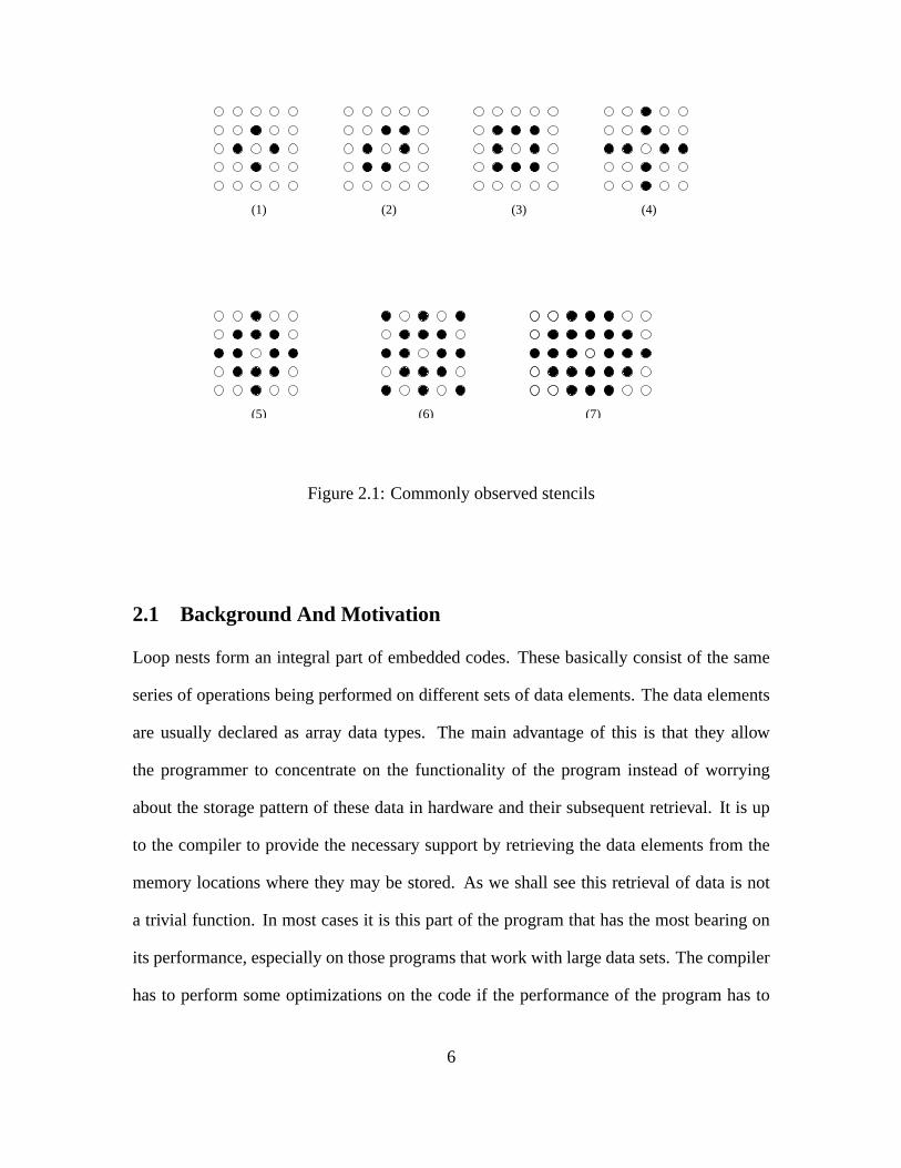
2.1 Commonly observed stencils . . . . . . . . . . . . . . . . . . . . . . . . . 6
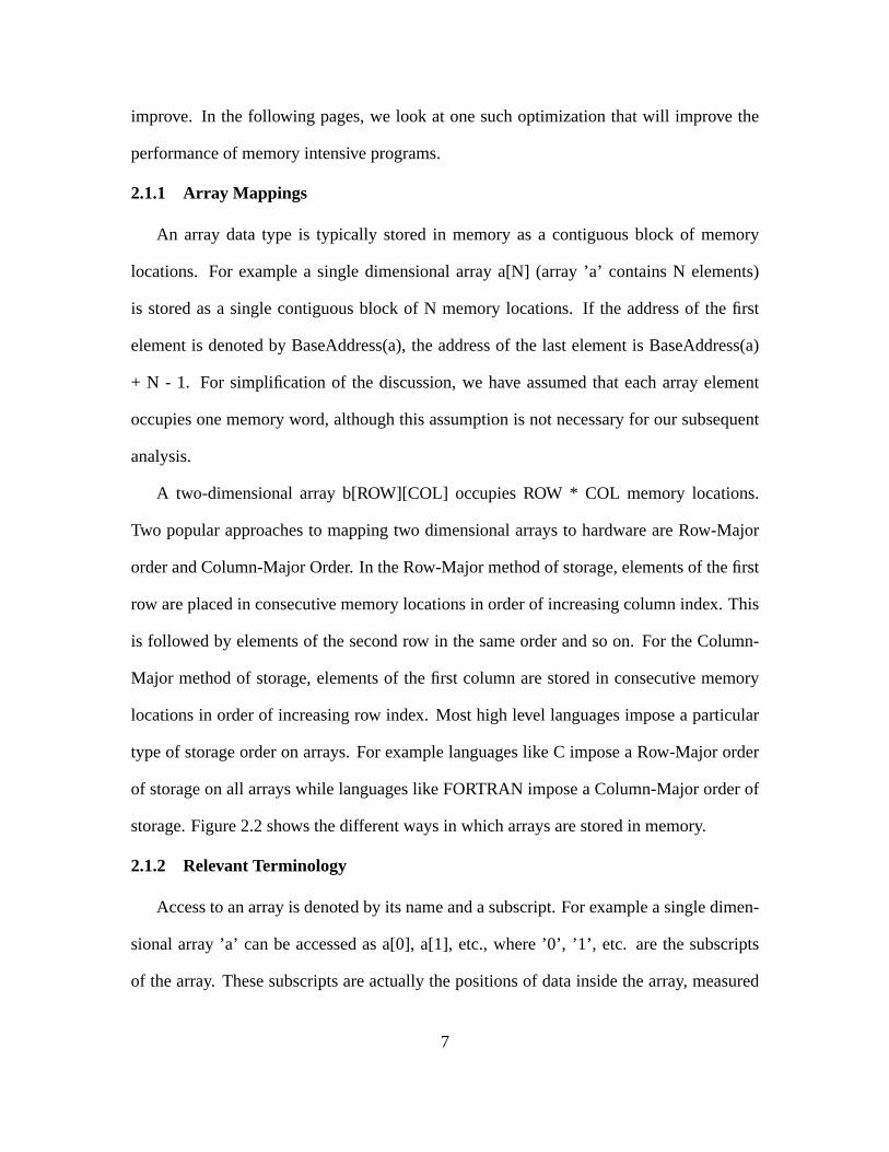
2.2 Storage pattern of arrays in memory . . . . . . . . . . . . . . . . . . . . . 8
2.3 Motivating example: 7-point stencil . . . . . . . . . . . . . . . . . . . . . 9
2.4 Access pattern for the motivating example . . . . . . . . . . . . . . . . . . 12
2.5 Results for the 9 point cross stencil. . . . . . . . . . . . . . . . . . . . . . 15
2.6 Results for the 9 point cross stencil when compiled with ’-fast’ option. . . . 16
2.7 Results for the 13 point star stencil. . . . . . . . . . . . . . . . . . . . . . . 17
2.8 Results for the 13 point star stencil when compiled with ’-fast’ option. . . . 18
2.9 Results for the hexagonal stencil. . . . . . . . . . . . . . . . . . . . . . . . 19
2.10 Results for the hexagonal stencil when compiled with ’-fast’ option. . . . . 20
2.11 Results for the 19 point asymmetric stencil. . . . . . . . . . . . . . . . . . 21
2.12 Results for the 19 point asymmetric stencil when compiled with ’-fast’ option. 22
2.13 Results for the 14 point irregular stencil. . . . . . . . . . . . . . . . . . . . 23
2.14 Results for the 14 point irregular stencil when compiled with ’-fast’ option. 24
2.15 Results for the 7 point array stencil when compiled with ’-fast’ option. . . . 25
3.1 Statement level dependence graph for Example 3.1 . . . . . . . . . . . . . 36
3.2 Statement level dependence graph for Example 3.2 . . . . . . . . . . . . . 38
v

3.3 Statement level dependence graph for Example 3.3 . . . . . . . . . . . . . 40
4.1 Illustration of the uniform redundancy of the dependence(1, 1) for Exam-ple 4.1 . . . . . . . . . . . . . . . . . . . . . . . . . . . . . . . . . . . . . 47
4.2 Illustration of the non-uniform redundancy of the dependence(1, 1) forExample 4.2 . . . . . . . . . . . . . . . . . . . . . . . . . . . . . . . . . . 47
4.3 2-dimensional iteration space and dependence vectors . . . . . . . . . . . . 51
4.4 Illustration of redundancy with multiple distance vectors. . . . . . . . . . . 63
5.1 Notation used in this chapter . . . . . . . . . . . . . . . . . . . . . . . . . 74
vi

ABSTRACT
Exploiting parallelism in loops in programs is an important factor in realizing the po-
tential performance of processors today. This dissertation develops and evaluates several
compiler optimizations aimed at improving the performance of loops on processors.
An important feature of a class of scientific computing problems is the regularity exhib-
ited by their access patterns. Chapter 2 presents an approach of optimizing the address gen-
eration of these problems that results in the following: (i) elimination of redundant arith-
metic computation by recognizing and exploiting the presence of common sub-expressions
across different iterations in stencil codes; and (ii) conversion of as many array references
to scalar accesses as possible, which leads to reduced execution time, decrease in address
arithmetic overhead, access to data in registers as opposed to caches, etc.
With the advent of VLIW processors, the exploitation of fine-grain instruction-level
parallelism has become a major challenge to optimizing compilers. Fine-grain scheduling
of inner loops has received a lot of attention, little work has been done in the area of
applying it to nested loops. Chapter 3 presents an approach to fine-grain scheduling of
nested loops by formulating the problem of finding the minimum iteration initiation interval
as one of finding a rational affine schedule for each statement in the body of a perfectly
nested loop which is then solved using linear programming.
Frequent synchronization on multiprocessors is expensive due to its high cost. Chapter
4 presents a method for eliminating redundant synchronization for nested loops. In nested
loops, a dependence may be redundant in only a portion of the iteration space. A charac-
vii
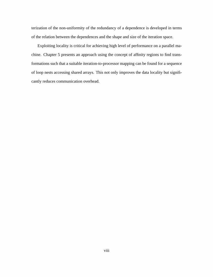
terization of the non-uniformity of the redundancy of a dependence is developed in terms
of the relation between the dependences and the shape and size of the iteration space.
Exploiting locality is critical for achieving high level of performance on a parallel ma-
chine. Chapter 5 presents an approach using the concept of affinity regions to find trans-
formations such that a suitable iteration-to-processor mapping can be found for a sequence
of loop nests accessing shared arrays. This not only improves the data locality but signifi-
cantly reduces communication overhead.
viii

CHAPTER 1
INTRODUCTION
Exploiting parallelism in loops in programs is an important factor in realizing the po-
tential performance of processors, both general-purpose and embedded, today. Program-
ming these machines remains a difficult problem. Much progress has been made result-
ing in a suite of techniques that extract coarse-grain parallelism from sequential programs
[3, 59, 76, 79]. This dissertation addresses several problems in improving the performance
of processors.
An important class of problems used widely in scientific computing and other applica-
tion domains perform memory intensive computations on large data sets. These data sets
get to be typically stored in main memory. The storage of these data sets in memory means
that the compiler needs to generate the address of a memory location in order to store these
data elements and generate the same address again when they are subsequently retrieved.
This operation of memory address computation is quite resource-intensive and degrades the
overall performance significantly if not performed efficiently. An important feature of the
class of problems considered in this chapter is the regularity exhibited by their access pat-
terns. In Chapter 2, we present an approach of optimizing the address generation of these
stencil problems. Our approach makes use of the observation that in all these stencils, a
significant fraction of the elements accessed are stored close to one other in memory. The
main contributions of the proposed technique is an optimization technique that results in the
following: (i) eliminating redundant arithmetic computation by recognizing and exploiting
the presence of common sub-expressions across different iterations in stencil codes; and
1

(ii) conversion of as many array references to scalar accesses as possible, which leads to
reduced execution time, decrease in address arithmetic overhead, access to data in registers
as opposed to caches, etc.
With the advent of VLIW processors, the exploitation of fine-grain instruction-level
parallelism has become a major challenge to parallelizing compilers [18, 63].Software
pipelining [1, 15, 42] has been proposed as an effective fine-grain scheduling technique
that restructures the statements in the body of a loop subject to resource and dependence
constraints such that one iteration of a loop can start execution before another finishes.
The total execution time thus depends on the rate at which new iterations start executing.
While software pipelining of inner loops has received a lot of attention, little work has
been done in the area of applying it to nested loops. Chapter 3 presents an approach to fine-
grain scheduling of nested loops by presenting a technique to find the minimum iteration
initiation interval (in the absence of resource constraints). We formulate the problem as one
of finding a rational affine schedule for each statement in the body of a perfectly nested loop
which is then solved using linear programming. This framework allows for an integrated
treatment of iteration-dependent statement reordering and multidimensional loop unrolling.
In contrast to most work in scheduling nested loops, we treat each statement in the body
as a unit of scheduling. Thus, the schedules derived allow for instances of statements
from different iterations to be scheduled at the same time. Optimal schedules derived here
subsume extant work on software pipelining of inner loops.
In order to achieve maximal parallel execution, a program must be decomposed into
as many concurrent tasks as possible. The dependences in the original program must be
preserved in concurrent execution to guarantee correctness, often through the use of syn-
chronization instructions. Synchronization involves large overhead such as busy-waiting,
2
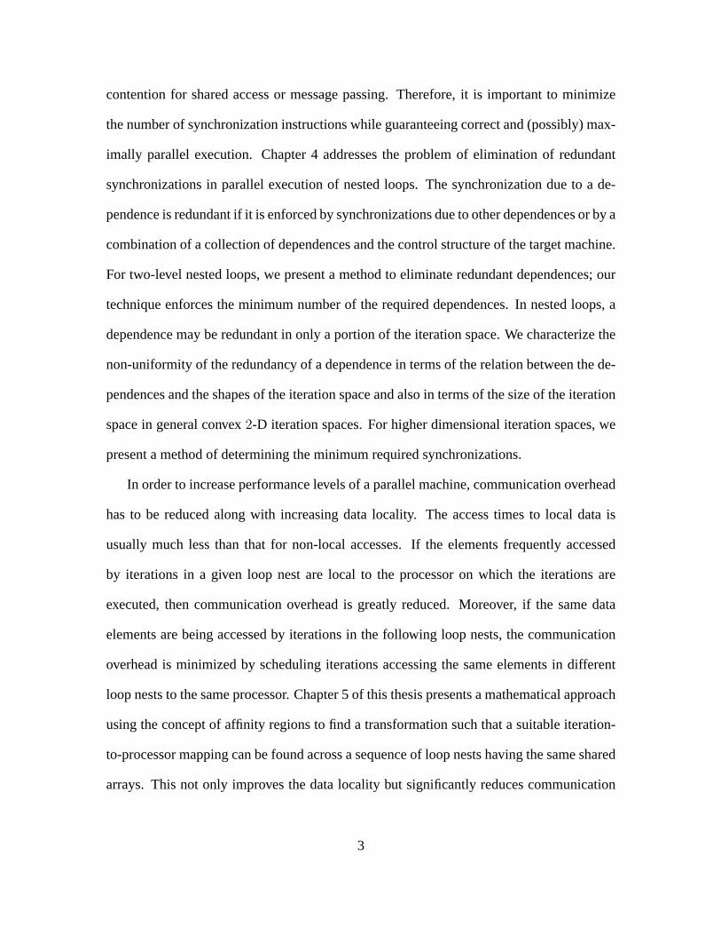
contention for shared access or message passing. Therefore, it is important to minimize
the number of synchronization instructions while guaranteeing correct and (possibly) max-
imally parallel execution. Chapter 4 addresses the problem of elimination of redundant
synchronizations in parallel execution of nested loops. The synchronization due to a de-
pendence is redundant if it is enforced by synchronizations due to other dependences or by a
combination of a collection of dependences and the control structure of the target machine.
For two-level nested loops, we present a method to eliminate redundant dependences; our
technique enforces the minimum number of the required dependences. In nested loops, a
dependence may be redundant in only a portion of the iteration space. We characterize the
non-uniformity of the redundancy of a dependence in terms of the relation between the de-
pendences and the shapes of the iteration space and also in terms of the size of the iteration
space in general convex2-D iteration spaces. For higher dimensional iteration spaces, we
present a method of determining the minimum required synchronizations.
In order to increase performance levels of a parallel machine, communication overhead
has to be reduced along with increasing data locality. The access times to local data is
usually much less than that for non-local accesses. If the elements frequently accessed
by iterations in a given loop nest are local to the processor on which the iterations are
executed, then communication overhead is greatly reduced. Moreover, if the same data
elements are being accessed by iterations in the following loop nests, the communication
overhead is minimized by scheduling iterations accessing the same elements in different
loop nests to the same processor. Chapter 5 of this thesis presents a mathematical approach
using the concept of affinity regions to find a transformation such that a suitable iteration-
to-processor mapping can be found across a sequence of loop nests having the same shared
arrays. This not only improves the data locality but significantly reduces communication
3
overhead. Since the concept of affinity regions is being used, the schedule of the first
loop nest in the affinity region is saved and used by other nests in the affinity region. The
iterations of the first loop nest can be scheduled by the compiler and the only overhead
involved is in saving this schedule for subsequent loop nests in the affinity region. In this
work we consider cases that include single as well as two shared arrays across loop nests,
illustrated with examples, where the dimensionality of the shared array and the level of
nesting in the loop nests are different.
4
CHAPTER 2
ADDRESS CODE AND ARITHMETIC OPTIMIZATIONS
An important class of problems used widely in both the embedded systems and scien-
tific domains perform memory intensive computations on large data sets. These data sets
get to be typically stored in main memory. The storage of these data sets in memory means
that the compiler needs to generate the address of a memory location in order to store these
data elements and generate the same address again when they are subsequently retrieved.
As we shall see, this operation of memory address computation is quite resource intensive
and degrades the overall performance significantly if not performed efficiently.
An important feature of the class of problems considered in this chapter is the regu-
larity exhibited by their access patterns. A regular problem can be characterized by its
corresponding stencil. Figure 2.1 illustrates some of the commonly found stencils.
In this chapter, we present an approach of optimizing the address generation of these
stencil problems. Our approach makes use of the observation that in all these stencils, a
significant fraction of the elements accessed are stored close to one other in memory. The
main contributions of the proposed technique is an optimization technique that results in
the following:
• eliminating redundant arithmetic computation by recognizing and exploiting the pres-
ence of common sub-expressions across different iterations in stencil codes; and
• conversion of as many array references to scalar accesses as possible, which leads
to reduced execution time, decrease in address arithmetic overhead, access to data in
registers as opposed to caches, etc.
5
����
����
����
����
��
��
��
����
����
����
����
����
����
����
����
����
!!
""##
$$%%
&&''
(())
**++
,,--
..//
0011
2233
4455
6677
8899
::;;
<<==
>>??
@@AA
BBCC
DDEE
FFGG
HHII
JJKK
LLMM
NNOO
PPQQ
RRSS
TTUU
VVWW
XXYY
ZZ[[
\\]]
^^__
``aa
bbcc
ddee
ffgg
hhii
jjkk
llmm
nnoo
ppqq
rrss
ttuu
vvww
xxyy
zz{{
||}}
~~��
����
����
����
����
����
����
����
����
����
����
����
����
(1) (2) (3) (4)
(5) (6) (7)
Figure 2.1: Commonly observed stencils
2.1 Background And Motivation
Loop nests form an integral part of embedded codes. These basically consist of the same
series of operations being performed on different sets of data elements. The data elements
are usually declared as array data types. The main advantage of this is that they allow
the programmer to concentrate on the functionality of the program instead of worrying
about the storage pattern of these data in hardware and their subsequent retrieval. It is up
to the compiler to provide the necessary support by retrieving the data elements from the
memory locations where they may be stored. As we shall see this retrieval of data is not
a trivial function. In most cases it is this part of the program that has the most bearing on
its performance, especially on those programs that work with large data sets. The compiler
has to perform some optimizations on the code if the performance of the program has to
6
improve. In the following pages, we look at one such optimization that will improve the
performance of memory intensive programs.
2.1.1 Array Mappings
An array data type is typically stored in memory as a contiguous block of memory
locations. For example a single dimensional array a[N] (array ’a’ contains N elements)
is stored as a single contiguous block of N memory locations. If the address of the first
element is denoted by BaseAddress(a), the address of the last element is BaseAddress(a)
+ N - 1. For simplification of the discussion, we have assumed that each array element
occupies one memory word, although this assumption is not necessary for our subsequent
analysis.
A two-dimensional array b[ROW][COL] occupies ROW * COL memory locations.
Two popular approaches to mapping two dimensional arrays to hardware are Row-Major
order and Column-Major Order. In the Row-Major method of storage, elements of the first
row are placed in consecutive memory locations in order of increasing column index. This
is followed by elements of the second row in the same order and so on. For the Column-
Major method of storage, elements of the first column are stored in consecutive memory
locations in order of increasing row index. Most high level languages impose a particular
type of storage order on arrays. For example languages like C impose a Row-Major order
of storage on all arrays while languages like FORTRAN impose a Column-Major order of
storage. Figure 2.2 shows the different ways in which arrays are stored in memory.
2.1.2 Relevant Terminology
Access to an array is denoted by its name and a subscript. For example a single dimen-
sional array ’a’ can be accessed as a[0], a[1], etc., where ’0’, ’1’, etc. are the subscripts
of the array. These subscripts are actually the positions of data inside the array, measured
7

X
Row Major Order Column Major Order
Single dimensional storage
X + N − 1
Figure 2.2: Storage pattern of arrays in memory
from the beginning of the array. Thus the access a[i] is the access to a data at a distance
of ’i’ elements from the start of the array. The memory address where a[i] is stored can be
calculated as:
BaseAddress(a) + i. (2.1)
A two-dimensional array has both a length and a breadth and its access is denoted by b[i][j],
where ’i’ is the row subscript and ’j’ is the column subscript. Again the memory address
where b[i][j] is stored can be calculated as:
BaseAddress(b) + (number of columns in b ∗ i) + j. (2.2)
This method of address calculation assumes a row major order of memory storage. This
assumption is followed throughout this chapter unless mentioned otherwise.
2.1.3 Performance Issues
Most memory intensive applications are characterized by some common features such
as loop nests and the usage of large data blocks that are usually stored in memory as arrays.
8
Iteartion 1
Iteration 2
Iteration 3
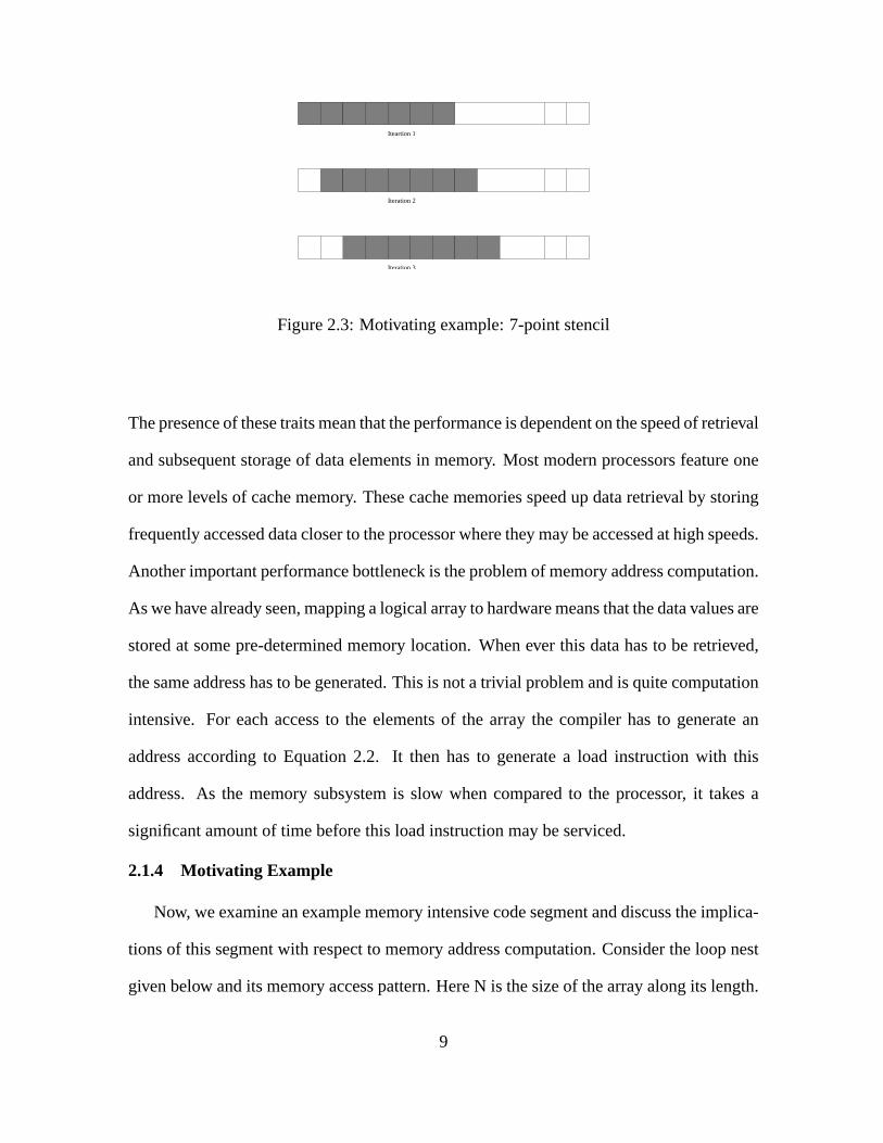
Figure 2.3: Motivating example: 7-point stencil
The presence of these traits mean that the performance is dependent on the speed of retrieval
and subsequent storage of data elements in memory. Most modern processors feature one
or more levels of cache memory. These cache memories speed up data retrieval by storing
frequently accessed data closer to the processor where they may be accessed at high speeds.
Another important performance bottleneck is the problem of memory address computation.
As we have already seen, mapping a logical array to hardware means that the data values are
stored at some pre-determined memory location. When ever this data has to be retrieved,
the same address has to be generated. This is not a trivial problem and is quite computation
intensive. For each access to the elements of the array the compiler has to generate an
address according to Equation 2.2. It then has to generate a load instruction with this
address. As the memory subsystem is slow when compared to the processor, it takes a
significant amount of time before this load instruction may be serviced.
2.1.4 Motivating Example
Now, we examine an example memory intensive code segment and discuss the implica-
tions of this segment with respect to memory address computation. Consider the loop nest
given below and its memory access pattern. Here N is the size of the array along its length.
9
for i = 3 toN − 4 do
b[i] = ( a[i-3] + a[i-2] + a[i-1] + a[i] + a[i+1] + a[i+2] + a[i+3]) / 7
Such loop nests are called stencil codes because they compute values using neighbor-
ing array elements in a fixed stencil pattern. This stencil pattern of data accesses is then
repeated for each element of the array. For instance, the above loop nest consists of a
simple 7 point stencil in one dimensions as shown in Figure 2.3. On each loop iteration,
seven neighboring elements of the array are accessed and their sum calculated. As the com-
putation progresses, the stencil pattern is repeatedly applied to array elements in the row,
sweeping through the array. Such kind of loop nests are very popular in image processing
applications.
At first glance, it is immediately obvious that we are trying to access 7 elements of
the single dimensional array ’a’ , all at different locations, in successive iterations. Thus
we need to perform 7 address computations to retrieve the data from the memory. Most
traditional compilers tend to store the base address of array ’a’ in a register. Access to
different elements of this array means the computation of the memory addresses using
Equation 2.1. The computation of the sum of these 7 elements is also not a trivial operation.
Since these operations need to be performed for each iteration of the loop, the number of
total computations to be performed for even small values of N is quite exhaustive and could
degrade performance if not performed efficiently.
2.2 Related Work on Address Overhead Reduction
Specialized hardware has been used for reducing address arithmetic overheads [37], but this
leads to increased design complexity and cost. In addition, several authors have addressed
the problem of laying out scalar variables to make effective use of address generation units
in embedded processors [45]. The IMEC group has used several transformations and ad-
10

vocated the use of special hardware for reducing the effect of address arithmetic overhead
[11, 14, 53, 54]. Gupta et al. [23] have used induction variable analysis and optimization
to improve the performance of address arithmetic.
Callahan et al. [9] (and Liu’s group [48, 49]) present a technique for register allocation
of subscripted variables. They argue that most compilers do not allocate array elements to
registers because standard data-flow analysis make it difficult to analyze the definitions and
uses of individual array elements. They then discuss an approach of replacing subscripted
variables by scalars to effect reuse. The subsequent code is then modified to use the data
elements stored in these scalars. The advantage of this approach is that all array variables
are replaced by scalars that are then mapped to registers. In successive iterations, those
variables which are reused can be accessed from registers directly. This improves perfor-
mance because it eliminates the address calculation overhead. Replacing array variables
by scalars means that the cache configuration does not degrade performance significantly.
This is because all variables that are reused are present in registers and reused data is no
longer accessed via the cache mechanism. This approach does improve the performance
to a large extent. However the arithmetic overhead involving the actual data elements still
remains. Another problem is that of register pressure. By mapping the scalars to registers,
we use up a lot of registers. If the amount of reuse is large, the register pressure builds up
and can significantly degrade the performance.
In contrast to these works, we have proposed a technique that
• eliminates redundant arithmetic computation by recognizing and exploiting the pres-
ence of common sub-expressions across different iterations in stencil codes; and
• converts as many array references to scalar accesses as possible, which leads to a
significant improvement.
11
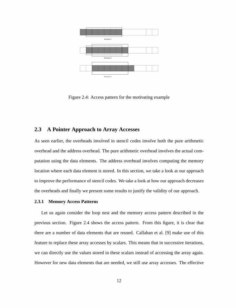
Iteration 2
Iteration 3
Iteartion 1
Figure 2.4: Access pattern for the motivating example
2.3 A Pointer Approach to Array Accesses
As seen earlier, the overheads involved in stencil codes involve both the pure arithmetic
overhead and the address overhead. The pure arithmetic overhead involves the actual com-
putation using the data elements. The address overhead involves computing the memory
location where each data element is stored. In this section, we take a look at our approach
to improve the performance of stencil codes. We take a look at how our approach decreases
the overheads and finally we present some results to justify the validity of our approach.
2.3.1 Memory Access Patterns
Let us again consider the loop nest and the memory access pattern described in the
previous section. Figure 2.4 shows the access pattern. From this figure, it is clear that
there are a number of data elements that are reused. Callahan et al. [9] make use of this
feature to replace these array accesses by scalars. This means that in successive iterations,
we can directly use the values stored in these scalars instead of accessing the array again.
However for new data elements that are needed, we still use array accesses. The effective
12

goal of the code segment described in the previous section is to calculate the sum of seven
data elements, the elements moving along the array across successive iterations. From
Figure 2.4, another thing that can be seen is that as many as six data elements are reused
across any two iterations. This means that the sum of these six elements is a common
sub-expression in the arithmetic computation across any two successive iterations. If we
were to store the value of the common sub-expression in a register, then across iterations
the amount of arithmetic computation needed would be greatly decreased. Storing the
common sub-expression in a register also decreases the number of scalars that we operate
with. This correspondingly means that there is almost no register pressure unlike the other
approaches that we described. In each iteration, we also access the new data elements
that we need using pointers instead of array accesses. This helps a lot in improving the
performance because the memory address computation overhead that we described has
now been eliminated.
2.3.2 The Algorithm
Here is the algorithm and it consists of the following steps:
1. From the access pattern of the loop, find the common sub-expression (CSE) across
any two successive iterations.
2. Initialize the CSE at the beginning of the loop body.
3. Modify the loop body to use the value of this CSE.
4. In each iteration, update the value of the CSE.
5. Replace all array accesses by pointer dereferences.
Given a loop nest, the algorithm first looks at the access pattern of the array elements
involved. From this access pattern, we pick out the common sub-expression that exists
13
between any two successive iterations. This common sub-expression is effectively a scalar
variable that has been mapped to a register. This scalar is initialized at the beginning of
the code segment. The rest of the code is then modified to use the value of the common
sub-expression. Using this value means that the amount of arithmetic computation involved
is decreased significantly. The common sub-expression is also updated in each iteration.
New data elements that are needed in each iteration are accessed by pointer dereferences.
Using pointers to access data elements improves the performance by reducing the memory
address computation overhead. This approach to stencil codes makes full utilization of the
spatial locality exhibited by these stencil codes.
2.3.3 Experimental Results
We made the modifications as determined by our algorithm on several scientific prob-
lems exhibiting regular computational patterns. Most of these patterns are given in Sec-
tion 2.1. We also modified the loop nests by using Callahan et al.’s approach [9]. The loop
nests were then compiled using the ’cc’ compiler and we ran the executables on the Ultra
SPARC workstations. The compiler options that we used were cc and cc -fast. Compil-
ing the code using only the default compiler options generates executables, where the main
goal of the compiler is to reduce the cost of compilation. Compiling using the ’-fast’ option
selects the optimum combination of compiler options for speed. This provides close to the
best performance for most realistic applications.
The original and modified codes were then timed over 100 runs and averaged. We in-
creased the array dimensions over a wide range of values and measured performance over
this range. We plotted graphs for the original code and the modified codes using both Calla-
han et al.’s approach and ours. This helps us to compare the performance improvements on
the original code as a result of the optimizations using both the approaches. On the X-axis
14
����
����
����
����
��
��
��
����
9 point cross stencil
Our Approach.
Callahan Approach.
Original Code.
1000 1500 2000 2500 3000 3500 40000
1
2
3
4
5
6
7
Array Dimension
Tim
e in
sec
onds
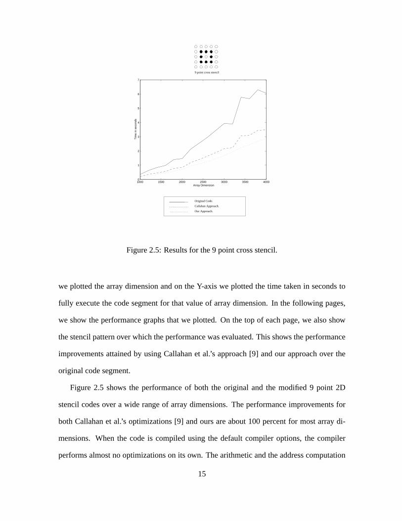
Figure 2.5: Results for the 9 point cross stencil.
we plotted the array dimension and on the Y-axis we plotted the time taken in seconds to
fully execute the code segment for that value of array dimension. In the following pages,
we show the performance graphs that we plotted. On the top of each page, we also show
the stencil pattern over which the performance was evaluated. This shows the performance
improvements attained by using Callahan et al.’s approach [9] and our approach over the
original code segment.
Figure 2.5 shows the performance of both the original and the modified 9 point 2D
stencil codes over a wide range of array dimensions. The performance improvements for
both Callahan et al.’s optimizations [9] and ours are about 100 percent for most array di-
mensions. When the code is compiled using the default compiler options, the compiler
performs almost no optimizations on its own. The arithmetic and the address computation
15

����
����
����
����
��
��
��
����
Our Approach.
Callahan Approach.
Original Code.
1000 1500 2000 2500 3000 3500 40000
0.2
0.4
0.6
0.8
1
1.2
1.4
1.6
Array Dimension
Tim
e in
sec
onds
9 point cross stencil
Figure 2.6: Results for the 9 point cross stencil when compiled with ’-fast’ option.
overheads are quite huge and have a large impact on the performance. The optimized codes
on the other hand, perform much better because the overheads have been reduced to a large
extent. We can see that our approach at optimizing the code results in an improvement of
about10% to 20% for most array dimensions. This is because, we have reduced the pure
arithmetic overhead to a larger extent than that was done by the other approach.
Figure 2.6 shows the performance when the code is compiled using the ’-fast’ option.
Using this option generates the best possible performance for any code on the target ma-
chine. The compiler performs some optimizations on its own with a view of improving
the overall performance. Hence, here we can see that the time taken to execute the stencil
codes has improved for even the naive code. Here too our approach performs better than
16
����
����
����
����
��
��
��
����
����
����
����
����
Our Approach.
Callahan Approach.
Original Code.
1000 1500 2000 2500 3000 3500 40000
1
2
3
4
5
6
7
8
9
Array Dimension
Tim
e in
sec
onds
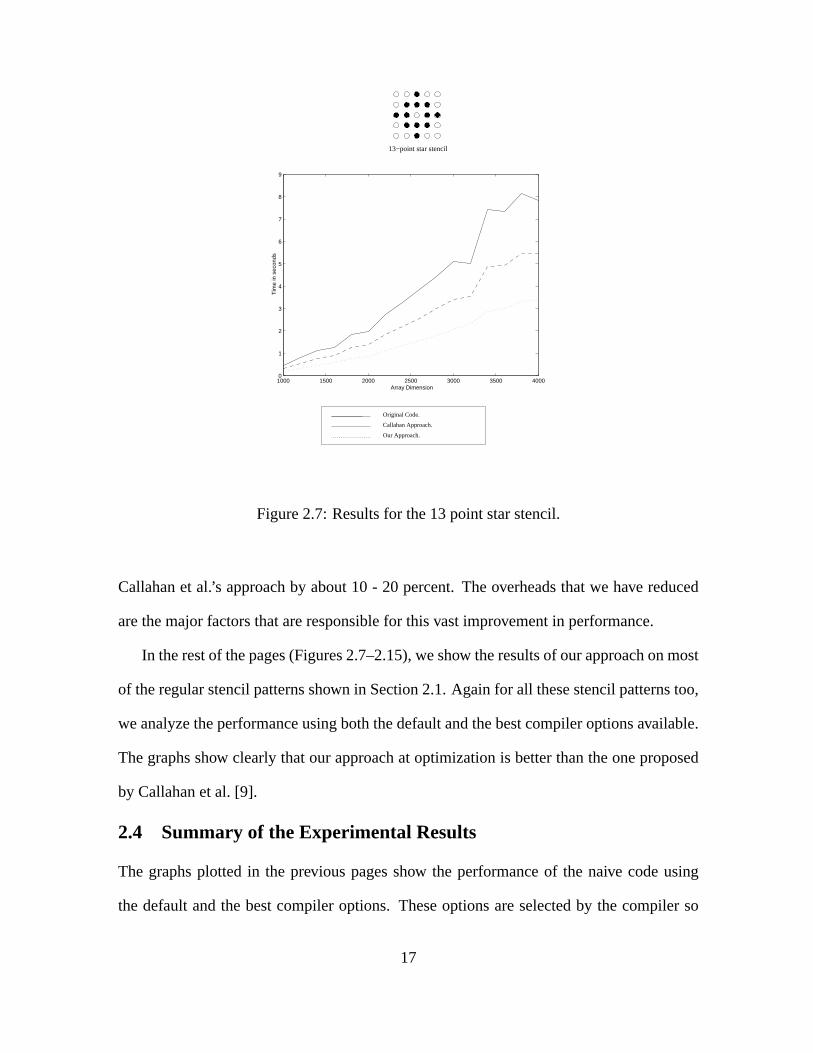
13−point star stencil
Figure 2.7: Results for the 13 point star stencil.
Callahan et al.’s approach by about 10 - 20 percent. The overheads that we have reduced
are the major factors that are responsible for this vast improvement in performance.
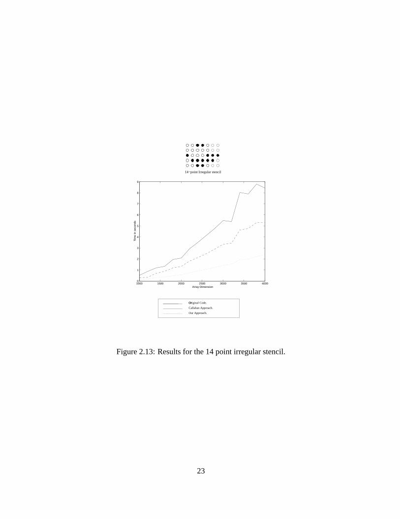
In the rest of the pages (Figures 2.7–2.15), we show the results of our approach on most
of the regular stencil patterns shown in Section 2.1. Again for all these stencil patterns too,
we analyze the performance using both the default and the best compiler options available.
The graphs show clearly that our approach at optimization is better than the one proposed
by Callahan et al. [9].
2.4 Summary of the Experimental Results
The graphs plotted in the previous pages show the performance of the naive code using
the default and the best compiler options. These options are selected by the compiler so
17
����
����
����
����
��
��
��
����
����
����
����
����
����
����
����
����
!!
""##
$$%%
&&''
(())
**++
,,--
..//
Our Approach.
Callahan Approach.
Original Code.
1000 1500 2000 2500 3000 3500 40000
0.2
0.4
0.6
0.8
1
1.2
1.4
1.6
1.8
Array Dimension
Tim
e in
sec
onds
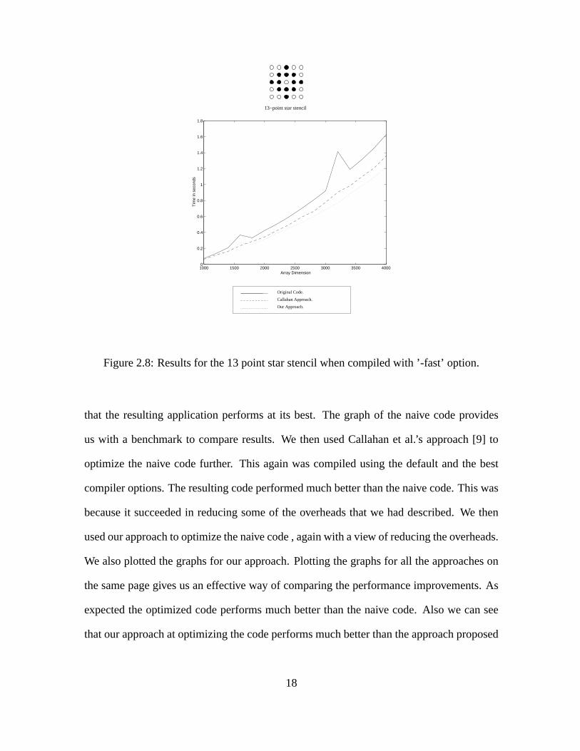
13−point star stencil
Figure 2.8: Results for the 13 point star stencil when compiled with ’-fast’ option.
that the resulting application performs at its best. The graph of the naive code provides
us with a benchmark to compare results. We then used Callahan et al.’s approach [9] to
optimize the naive code further. This again was compiled using the default and the best
compiler options. The resulting code performed much better than the naive code. This was
because it succeeded in reducing some of the overheads that we had described. We then
used our approach to optimize the naive code , again with a view of reducing the overheads.
We also plotted the graphs for our approach. Plotting the graphs for all the approaches on
the same page gives us an effective way of comparing the performance improvements. As
expected the optimized code performs much better than the naive code. Also we can see
that our approach at optimizing the code performs much better than the approach proposed
18

����
����
����
����
��
��
��
����
����
����
����
����
����
����
����
����
!!
""##
$$%%
&&''
(())
**++
Hexagonal Stencil
Our Approach.
Callahan Approach.
Original Code.
1000 1500 2000 2500 3000 3500 40000
5
10
15
Array Dimension
Tim
e in
sec
onds
Figure 2.9: Results for the hexagonal stencil.
by Callahan et al. The performance improvement between these two approaches is as much
as 10-20 percent for most array dimensions.
2.5 Chapter Summary
In this chapter, we focused on optimizing codes that exhibit regular access patterns. These
codes are called stencil codes. These code segments have two major overheads: (i) the
pure arithmetic computation overhead and (ii) the memory address computation overhead.
These overheads determine the performance of these code segments. Callahan et al. [9] pro-
pose an approach to optimize these stencil codes and thereby improve their performance.
They replace all subscripted array variables by scalars, thereby effecting reuse of these
scalar variables. These scalar variables are then mapped to registers. Subsequent reuse
19

����
����
����
����
��
��
��
����
����
����
����
����
����
����
����
����
!!
""##
$$%%
&&''
(())
**++
Hexagonal Stencil
Our Approach.
Callahan Approach.
Original Code.
1000 1500 2000 2500 3000 3500 40000
0.5
1
1.5
2
2.5
3
3.5
Array Dimension
Tim
e in
sec
onds
Figure 2.10: Results for the hexagonal stencil when compiled with ’-fast’ option.
of these data elements means that they can be directly accessed from registers instead of
through the cache mechanism. This means that loads of all reused data elements can be
serviced at processor speed instead of having to deal with cache conflicts and subsequent
loads from secondary memory. This approach results in a good improvement in perfor-
mance because the memory address computation overhead has been reduced. However the
major disadvantage with this approach is that because of the large number of data elements
that might be reused, the number of scalars that will be needed is also large. This creates a
lot of register pressure which then starts to degrade performance. Also this approach does
not seek to reduce the pure arithmetic computation overhead.
20
Our Approach.
Callahan Approach.
Original Code.
����
����
����
����
��
��
��
�������
�����
����
����
����
����
����
����
!!
""##
$$%%
&&''
(())**+
+,,--
..//
0011
2233
4455
6677
8899
::;;
<<==
>>??
@@AA
BBCCDDE
EFFGG
HHII
JJKK
LLMM
NNOO
PPQQ
RRSS
TTUU
VVWW
XXYY
ZZ[[
\\]]^^_
_``aa
bbcc
ddee
ffgg
hhii
jjkk
llmm
nnoo
ppqq
rrss
ttuu
vvwwxxy
yzz{{
||}}
~~��
����
����
����
����
����
����
����
����
�������
�����
����
����
����
1000 1500 2000 2500 3000 3500 40000
2
4
6
8
10
12
14
Array Dimension
Tim
e in
sec
onds
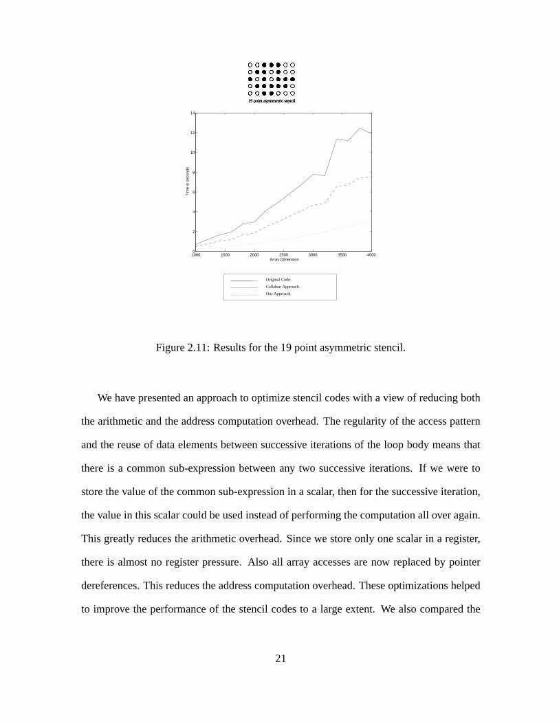
19 point asymmetric stencil19 point asymmetric stencil19 point asymmetric stencil
Figure 2.11: Results for the 19 point asymmetric stencil.
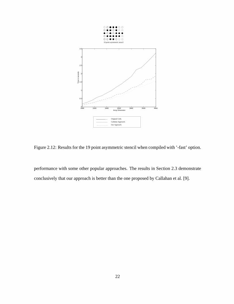
We have presented an approach to optimize stencil codes with a view of reducing both
the arithmetic and the address computation overhead. The regularity of the access pattern
and the reuse of data elements between successive iterations of the loop body means that
there is a common sub-expression between any two successive iterations. If we were to
store the value of the common sub-expression in a scalar, then for the successive iteration,
the value in this scalar could be used instead of performing the computation all over again.
This greatly reduces the arithmetic overhead. Since we store only one scalar in a register,
there is almost no register pressure. Also all array accesses are now replaced by pointer
dereferences. This reduces the address computation overhead. These optimizations helped
to improve the performance of the stencil codes to a large extent. We also compared the
21
Our Approach.
Callahan Approach.
Original Code.
19 point asymmetric stencil
����
����
����
����
��
��
��
�������
�����
����
����
����
1000 1500 2000 2500 3000 3500 40000
0.5
1
1.5
2
2.5
3
3.5
Array Dimension
Tim
e in
sec
onds
Figure 2.12: Results for the 19 point asymmetric stencil when compiled with ’-fast’ option.
performance with some other popular approaches. The results in Section 2.3 demonstrate
conclusively that our approach is better than the one proposed by Callahan et al. [9].
22
Our Approach.
Callahan Approach.
Original Code.
����
����
����
����
��
��
��
�������
�����
����
����
����
1000 1500 2000 2500 3000 3500 40000
1
2
3
4
5
6
7
8
9
Array Dimension
Tim
e in
sec
onds
14−point Irregular stencil
Or
Figure 2.13: Results for the 14 point irregular stencil.
23

Our Approach.
Callahan Approach.
Original Code.
����
����
����
����
��
��
��
�������
�����
����
����
����
14−point Irregular stencil
1000 1500 2000 2500 3000 3500 40000
0.2
0.4
0.6
0.8
1
1.2
1.4
1.6
Array Dimension
Tim
e in
sec
onds
Figure 2.14: Results for the 14 point irregular stencil when compiled with ’-fast’ option.
24

����
����
����
����
��
��
X
Our Approach.
Callahan Approach.
Original Code.
1 2 3 4 5 6 7 8 9 10 11
x 106
0
0.1
0.2
0.3
0.4
0.5
0.6
0.7
0.8
0.9
Array Dimension
Tim
e in
sec
onds
7 point array stencil.
Figure 2.15: Results for the 7 point array stencil when compiled with ’-fast’ option.
25
CHAPTER 3
FINE-GRAIN SCHEDULING OF NESTED LOOPS
With the advent of embedded VLIW digital signal processors, the exploitation of fine-
grain instruction-level parallelism has become a major challenge to parallelizing compil-
ers [18, 63].Software pipelining[1, 15, 42] has been proposed as an effective fine-grain
scheduling technique that restructures the statements in the body of a loop subject to re-
source and dependence constraints such that one iteration of a loop can start execution
before another finishes. The total execution time thus depends on theiteration initiation
interval. While software pipelining of inner loops has received a lot of attention, little work
has been done in the area of applying it to nested loops. This chapter presents an approach
to fine-grain scheduling of nested loops by presenting a technique to find the minimum iter-
ation initiation interval (in the absence of resource constraints). We formulate the problem
as one of finding a rational affine schedule for each statement in the body of a perfectly
nested loop which is then solved using linear programming. This framework allows for
an integrated treatment of iteration-dependent statement reordering and multidimensional
loop unrolling. In contrast to most work in scheduling nested loops, we treat each state-
ment in the body as a unit of scheduling. Thus, the schedules derived allow for instances
of statements from different iterations to be scheduled at the same time. Optimal schedules
derived here subsume extant work on software pipelining of inner loops.
3.1 Background
Good and thorough parallelization of a program critically depends on how precisely a com-
piler can discover the data dependence information [3, 8, 75, 76, 79]. These dependences
26
imply precedence constraints among computations which have to be satisfied for a correct
execution. In this chapter, we mainly consider perfectly nested loops of the form:
for I1 = L1 toU1 do· · ·
for In = Ln toUn doS1(I)· · ·Sr(I)
endfor· · ·
endfor
whereLj andUj are integer-valued affine expressions involvingI1, . . . , Ij−1 and I =
(I1, . . . , In). EachIj (j = 1, . . . , n) is a loop index;S1, . . . , Sr are assignment state-
ments of the formXo = E(X1, . . . , XK) whereXo is defined (i.e., written) in expression
E, which is evaluated using some variablesX1, X2, . . . , XK . We assume that the incre-
ment of each loop is+1. Each computation is denoted by an index vectorI = (I1, . . . , In).
A loop instance is the loop iteration where the indices take on a particular value,I = i =
(i1, i2, . . . , in). The instance of statementSk executed in iteration vectorI is denotedSk(I).
The iteration set is a collection of iteration vectors and constitutes the iteration space.
With the assumption on loop bound linearity, the sets of computations considered are finite
convex polyhedra of some iteration space inZn, wheren is the number of loops in the
nest which is also the dimensionality of the iteration space. The iteration set of a given
nested loop is described as a set of integer points (or, vectors) whose convex hullI is a
non-degenerate (or, full dimensional) convex polyhedron. The loop iterations are executed
in lexicographic ordering during sequential execution. Any vectorx = (x1, x2, . . . , xn) is a
positive vector,if its first (leading – read from left to right) non-zero component is positive
[8]. We say thati = (i1, . . . , in) precedesj = (j1, . . . , in), written i ≺ j, if j − i is a
27
positive vector. Positive vectors capture the lexicographic ordering among iterations of a
nested loop. A loop nest where the loop limits are constants is said to have a rectangular
iteration space associated with it.
Let X andY be twop-dimensional arrays; and letfi and gi (i = 1, . . . , p) be two
sets of integer functions such thatX(f1(I), . . . , fp(I)) is a “defined” (i.e.,written) variable
andY (g1(I), . . . , gp(I)) is a “used” (i.e., read) variable. LetF (I) denotef1(I), . . . , fp(I)
and letG(I) denoteg1(I), . . . , gp(I). Given two statementsSk(I1) andSl(I2), Sl(I2) is
dependent onSk(I1) (with distance vectordk,l) iff [8, 59, 75, 76]:
• (I1 ≺ I2) or (I1 = I2 andk < l) andfi(I1) = gi(I2) for i = 1, . . . , p;
• EitherX(F (I1)) is written in statementSk(I1) or X(G(I2)) is written in statement
Sl(I2).
A flow dependenceexists from statementSk to statementSl if Sk writes a value that is
subsequently, in sequential execution, read bySl. An anti-dependenceexists fromSk to
Sl if Sk reads a value that is subsequently modified bySl. An output dependenceexists
betweenSk andSl if Sk writes a value which is subsequently written bySl.
If I1 = I2, the dependence is called aloop-independent dependence;otherwise, it is
called aloop-carried dependence.Many dependences that occur in practice have a constant
distance in each dimension of the iteration space. In such cases, the vectord = I2 − I1 is
called thedistance vector.We limit our discussion to distance vectors in this chapter.
Dependence relations are often represented inStatement Level Dependence Graphs
(SLDG’s). For a perfectlyn-nested loop with index set(i1, i2, . . . , in) whose body contains
statementsS1, . . . , Sr, the SLDG hasr nodes, one for each statement. For each dependence
from statementSk to Sl with a distance vectordk,l, the graph has a directed edge from
nodeSk to Sl labeled with the distance vectordk,l. A dependence from a node to itself is
28
called aself-dependence.In addition to the three types of dependence mentioned above,
there is another type of dependence known ascontrol dependence. A control dependence
exists between a statement with a conditional jump and another statement if the conditional
jump statement controls the execution of the other statement. Control dependences can be
handled by methods similar to data dependences [3]. In our analysis, we treat the different
types of dependences uniformly. Methods to calculate data dependence vectors can be
found in [3, 8, 75, 76, 79].
3.2 Related Work on Fine-Grain Scheduling
Fine-grain scheduling of inner loops has been considered by several authors [1, 15, 19, 42,
77]. All of these studies search for the minimum iteration initiation interval by unrolling the
loop several times. This is inadequate in situations where the minimum iteration initiation
interval is non-integral. Moreover, these approaches use an ad hoc method to decide on the
degree of loop unrolling, and are unacceptable in cases where the optimal solution can be
found only after a very large amount of unrolling.
Aiken and Nicolau [2], describe a procedure which yields an optimal schedule for inner
sequential loops. The procedure works by simulating the execution of the loop body until a
pattern evolves. The technique does not guarantee an upper bound on the amount of time it
needs to find a solution. Zaky and Sadayappan [77] present a novel approach that is based
on eigenvalues of matrices that arise path algebra. Their algorithm has polynomial time
complexity; their algorithm exploits the connectivity properties of the loop dependence
graph. While the algorithm of [2] requires unrolling to detect a pattern, the algorithm in
[77] does not require any unrolling. Iwano and Yeh [30] use network flow algorithms for
optimal loops parallelization. fine-grain scheduling of sequential loops on limited resources
is discussed in [1, 42].
29
While fine-grain scheduling of inner loops has received a lot of attention, very few
authors have addressed fine-grain scheduling of nested loops. Cytron [12, 13] presents
a technique forDOACROSSloops that minimizes the delays between initiating successive
iterations of a sequential loop with no reordering of statements in its body. Cytron [12, 13]
does not explicitly attempt to exploit fine-grain parallelism. Munshi and Simmons [55]
study the problem of minimizing the iteration initiation interval which considers statement
reordering. They show that a close variant of the problem is NP-complete. Both these
papers separate the issues of iteration initiation and the scheduling of operations within an
iteration. In general, such a separation does not result in the minimum iteration initiation
interval.
Nicolau [57] suggestsloop quantizationas a technique for multidimensional loop un-
rolling in conjunction with tree-height reduction and percolation scheduling. He does not
consider the problem of determining the optimal initiation interval for each loop. Loop
quantization as described in [1, 57] deals with the problem at the iteration level rather than
at the statement level. Recently, Gaoet al. [20] present a technique that works for rectan-
gular loops but requires all components of all distance vectors to be positive. While uni-
modular transformations could be used to convert all distance vectors to have non-negative
entries, the transformed iteration spaces are no longer rectangular; this limits the appli-
cability of the results in [20]. The technique developed in this chapter does not have the
restriction on non-negativity and hence is more general.
3.3 Statement-Level Rational Affine Schedules
In this section, we formulate the problem of optimal fine grain scheduling of nested loops
in the absence of resource constraints as a Linear Programming (LP) problem [65] which
admits polynomial time solutions and is extremely fast in practice. This chapter generalizes
30
thehyperplanescheduling technique of scheduling iterations of nested loops pioneered by
Lamport [44] by deriving optimal schedules at the statement level rather than at the iteration
level. The solutions derived give the minimum iteration initiation interval for each level of
ann-nested loop. LetG denote the statement level dependence graph. IfG is acyclic, then
list scheduling and tree height reduction can be used to optimally schedule the computation
[1]. If G is cyclic, we use Tarjan’s algorithm [76, 79] to find all the strongly connected
components and schedule each strongly connected component separately. For now, we
discuss the optimal scheduling of a single strongly connected component inG. We plan to
explore the interleaving of the schedules of strongly connected components.
Given a numberx, bxc is the largest integer that is less than or equal tox and is called
thefloor of x. Let bqk(I)c denote the time at which statementSk(k = 1, . . . , r) in iteration
I = (i1, . . . , in) (denotedSk(I)) is scheduled which is the time at which execution starts.
Let tk be the time taken to execute statementSk. We assume thattk ≥ 1 and is an integer.
qk(I) is a rational function,i.e., it is written as
qk(I) = hk,1i1 + hk,2i2 + · · ·+ hk,nin + δk.
Let hk = (hk,1, hk,2, . . . , hk,n) for eachk; the elements of the vectorhk andδk are rational.
Note that we could also usedqk(I)e as the time at whichSk(I) is scheduled. We choose
to use the floor function throughout. We use a singleh vector for each strongly connected
component,i.e.,
qk(I) = h · I + δk k = 1, . . . , r.
The schedule should satisfy all the dependences in the loop. A schedule is a tuple〈h, δ〉whereh = (h1, . . . , hn) is ann-vector andδ = (δ1, . . . , δr) is anr-vector. A schedule
〈h, δ〉 is legal if for each edge from statementSk to Sl with a distance vectordk,l in G,
ql(I) ≥ qk(I − dk,l) + tk
31
This states that statementSl in iteration I can be scheduled only after statementSk in
iteration(I − dk,l) has completed execution. SinceSk(I − dk,l) starts execution atqk(I −
dk,l), Sl(I) can start at the earliest at timeqk(I − dk,l) + tk. Thus,
h · I + δl ≥ h · (I − dk,l) + δk + tk
h · dk,l ≥ δk − δl + tk
for all dependences inG. If dk,k is a self dependence onSk this condition translates to
h · dk,k ≥ tk
For ann-nested loop with a schedule〈h, δ〉, the execution time,E is given by the expres-
sion,
E = maxI,J∈I∧k,l∈[1,r]
{qk(I)− ql(J)}
The optimal execution time is the minimum value of the expressionE :
E ≈ maxI,J∈I{h · (I − J)}+ max
k∈[1,r](δk)− min
k∈[1,r](δk)
We assume that the number of iterations at each level of the loop nest is large; hence,
we ignore the contribution from the term:maxk∈[1,r](δk) −mink∈[1,r](δk). The expression
maxI,J∈I{h · (I − J)} can be approximated bymaxI∈I h · I − minI∈I h · I. With the
assumption that loop bounds are affine functions of outer loop variables, the iteration space
is a convex polyhedron. The extrema of affine functions overI, therefore occur at the
corners of the polyhedron [65]. If the iteration space is rectangular,i.e.,Lj andUj (j =
1, . . . , n) are integer constants, we can find an expression of the optimal value ofE using
Banerjee’s inequalities [8] as discussed below.
Definition 3.1 [8]: Given a numberh, its positive part,h+ = max(h, 0); and its negative
part,h− = max(−h, 0). Some properties are given below:
32
1. h+ ≥ 0 andh− ≥ 0
2. h = h+ − h− and abs(h) = h+ + h− (abs(h) is the absolute value ofh.)
3. −h− ≤ h ≤ h+
For rectangular loops, we assume thatLj ≤ ij ≤ Uj for j = 1, . . . , n andLj andUj
are constants. Using Banerjee’s inequalities,
maxI∈I
h · I =n∑j=1
{h+j Uj − h−j Lj
}
and
minI∈I
h · I =n∑j=1
{h+j Lj − h−j Uj
}
Therefore,
E ≈n∑j=1
{(h+j Uj − h−j Lj
)− (h+j Lj − h−j Uj
)}
E ≈n∑j=1
{(h+j + h−j
)(Uj − Lj)
}
From the properties in definition 3.1, this is equal to
E ≈n∑j=1
{abs(hj) (Uj − Lj)}
Thus, we can formulate the problem of finding the optimal schedule for ann-nested
loop (with a rectangular iteration space and the size of each level in the iteration space
is the same) withr-statements as that of finding a schedule〈h, δ〉, i.e., h1, . . . , hn and
δ1, . . . , δr that minimizes∑n
j=1 abs(hj) (Uj − Lj) subject to dependence constraints:
Minimizen∑j=1
abs(hj) (Uj − Lj)
subject to
h · dk,l ≥ δk − δl + tk k, l ∈ [1, r]
33
for every edge inG.
In many cases, the loop limits, though constants, are not known at compile time. In
such cases, we aim at finding optimal schedules independent of the loop limits. We assume
rectangular iteration spaces, where the size of each loopUj−Lj+1 is the same for all values
of j; in such cases, the optimal value of the expressionE is a function of∑n
j=1 abs(hj).
Thus, the execution time depends on the loop limits, where as the schedule,〈h, δ〉 does not
depend onLj andUj (j = 1, . . . , n). If the size,i.e.,the value ofUj−Lj+1 (j = 1, . . . , n),
are different for different loop levels, then the technique developed in this chapter is sub-
optimal. With unknown loop limits, our problem then is that of finding a schedule〈h, δ〉
that minimizes∑n
j=1 abs(hj) subject to dependence constraints:
Minimizen∑j=1
abs(hj)
subject to
h · dk,l ≥ δk − δl + tk k, l ∈ [1, r]
for every edge inG.
The above formulation is not in standard linear programming form for two reasons:
1. Lack of non-negativity constraints on〈h, δ〉
2. Absolute values of variables in the objective function
The first problem is handled by writing each variablehj(j = 1, . . . , n) andδi(i = 1, . . . , r)
as the difference of two variables, which are constrained to be non-negative,e.g.,replacehj
with h1j −h2
j with the constraint thath1j ≥ 0 andh2
j ≥ 0. The second problem is handled by
adding a set of variablesθj, j = 1, . . . , n; the new objective function is∑n
j=1 θj. For each
variablehj, we add two constraints,θj−hj ≥ 0 andθj +hj ≥ 0. With these modifications,
34

the problem is now in standard Linear Programming (LP) form:
Minimizen∑j=1
θj
subject to
θj − h1j + h2
j ≥ 0 j = 1, . . . , n
θj + h1j − h2
j ≥ 0 j = 1, . . . , nn∑j=1
((h1j − h2
j
)dk,lj
)− (δ1
k − δ2k
)+(δ1l − δ2
l
) ≥ tk
wherek, l ∈ [1, r] ∧ (k, l) ∈ edges(G).
The formulation has2n + m constraints with3n + 2r variables wherem is the number of
edges inG for ann-nested loop withr statements. In practice, our implementation obtains
solutions very quickly.
3.4 What Does the LP Solution Mean?
The value of abs(hj) denotes the iteration initiation interval for thejth loop in the nest.
If hj > 0, then the next loop iteration initiated at levelj is numbered higher than the
currently executing iteration at levelj. On the other handhj < 0 means that the next
iteration initiated has an iteration number less than the currently executing iteration, i.e.,
the loop at levelj is unrolled in the reverse direction. Ifhj =ajbj
whereaj and bj are
integers andgcd(aj, bj) = 1, in every abs(aj) time units, abs(bj) iterations at levelj are
unrolled; the unrolling is in reverse direction ifhj < 0. If hj = 0, the minimum iteration
initiation interval is zero, i.e., the loop is a parallel loop. Thus1abs(hj)denotes the initiation
or unrolling rate of thejth loop.
3.5 Examples
In this section, we show the effectiveness of our approach through examples. First, we show
an example of a two-level nested loop with four statements for which the optimal initiation
35

(1,-4)S3
S4
(0,1)
(1,-3)
(0,2)(1,3)
S1
S2
Figure 3.1: Statement level dependence graph for Example 3.1
rate (with no bound on resources) is determined using the LP formulation described in this
paper. Consider the following loop:
Example 3.1:for i = 1 toN do
for j = 1 toN doS1 : A[i, j] = B[i− 1, j − 3] +D[i− 1, j + 3]S2 : B[i, j] = C[i− 1, j + 4] +X[i, j]S3 : C[i, j] = A[i, j − 2] + Y [i, j]S4 : D[i, j] = A[i, j − 1] + Z[i, j]
endforendfor
The statement level dependence graph is shown in Figure 3.1. We assume that each
statement takes one unit of time to execute,i.e., t1 = t2 = t3 = t4 = 1. The linear
36
programming problem for this example is:
Minimize θ1 + θ2
subject to
θ1 − h11 + h2
1 ≥ 0
θ1 + h11 − h2
1 ≥ 0
θ2 − h12 + h2
2 ≥ 0
θ2 + h12 − h2
2 ≥ 0
2h12 − 2h2
2 − δ11 + δ2
1 + δ13 − δ2
3 ≥ 1
h11 − h2
1 − 4h12 + 4h2
2 − δ13 + δ2
3 + δ12 − δ2
2 ≥ 1
h11 − h2
1 + 3h12 − 3h2
2 − δ12 + δ2
2 + δ11 − δ2
1 ≥ 1
h12 − h2
2 − δ11 + δ2
1 + δ14 − δ2
4 ≥ 1
h11 − h2
1 − 3h12 + 3h2
2 − δ14 + δ2
4 + δ11 − δ2
1 ≥ 1
The optimal solution to this problem is:h1 = 85, h2 = −1
5, δ1 = 0, δ2 = 0, δ3 = 7
5, δ4 = 6
5.
This means that
• S1(i, j) is scheduled atb8i5− j
5c
• S2(i, j) is scheduled atb8i5− j
5c
• S3(i, j) is scheduled atb8i5− j
5+ 7
5c
• S4(i, j) is scheduled atb8i5− j
5+ 6
5c
In every 8 units of time, 5 new iterations of the outer loop are initiated. In every unit of
time, 5 new iterations of the inner loop are initiated in the reverse direction. The optimal
37

S1
0
S2S31
1
Figure 3.2: Statement level dependence graph for Example 3.2
execution time is≈ 9N5
. The best execution time that can be derived using only the iteration
space distance vectors is≈ 6N for the schedule5i + j. The fine grained solution runs3.3
times faster than the best solution that can be obtained using hyperplane technique [44].
The method presented here is equally applicable to inner loops. Consider the following
example from page 45 in [22].
Example 3.2:for i = 1 toN do
S1 : A[i] = C[i− 1]S2 : B[i+ 1] = A[i]S3 : C[i] = B[i]
endfor
The statement level dependence graph for Example 3.2 is shown in Figure 3.2. We
assume that each statement takes one unit of time to execute,i.e., t1 = t2 = t3 = 1. The
38
linear programming problem for this example is:
Minimize θ
subject to
θ − h1 + h2 ≥ 0
θ + h1 − h2 ≥ 0
0− δ11 + δ2
1 + δ12 − δ2
2 ≥ 1
h1 − h2 − δ12 + δ2
2 + δ13 − δ2
3 ≥ 1
h1 − h2 − δ13 + δ2
3 + δ11 − δ2
1 ≥ 1
The optimal solution to this problem is:h = 32, δ1 = 0, δ2 = 1, andδ3 = 1
2.
• S1(i) is scheduled atb3i2c
• S2(i) is scheduled atb3i2
+ 1c
• S3(i) is scheduled atb3i2
+ 12c
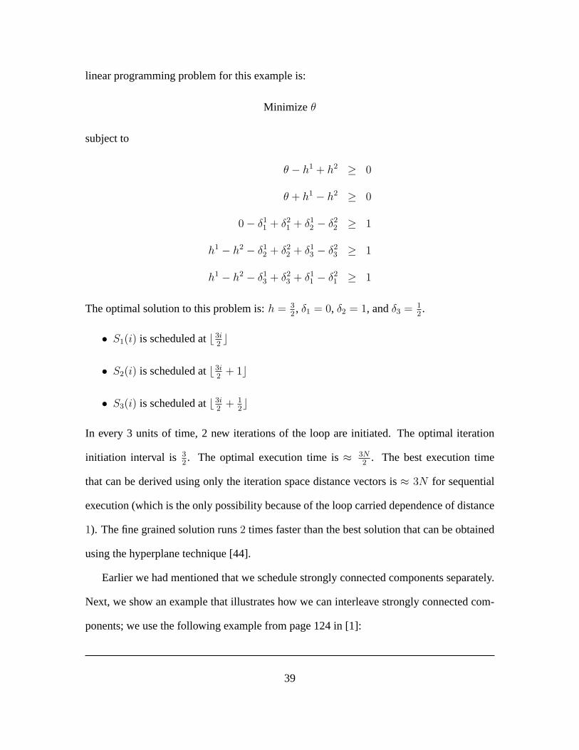
In every 3 units of time, 2 new iterations of the loop are initiated. The optimal iteration
initiation interval is 32. The optimal execution time is≈ 3N
2. The best execution time
that can be derived using only the iteration space distance vectors is≈ 3N for sequential
execution (which is the only possibility because of the loop carried dependence of distance
1). The fine grained solution runs2 times faster than the best solution that can be obtained
using the hyperplane technique [44].
Earlier we had mentioned that we schedule strongly connected components separately.
Next, we show an example that illustrates how we can interleave strongly connected com-
ponents; we use the following example from page 124 in [1]:
39

0 0
00
D
B
A
C
1 1
Figure 3.3: Statement level dependence graph for Example 3.3
Example 3.3:for i = 1 toN do
A : A[i] = f1(B[i])B : B[i] = f2(A[i], D[i− 1])C : C[i] = f3(A[i], D[i− 1])D : D[i] = f4(B[i], C[i])
endfor
The statement level dependence graph is shown in Figure 3.3. We assume that each
statement takes one unit of time to execute,i.e., t1 = t2 = t3 = t4 = 1. The SLDG in
Figure 3.3 has two strongly connected components, on consisting of just the nodeA and
the other made up of nodesB,C, andD. We use the same value ofh for all statements
in the loop; this allows for interleaving of different strongly connected components. The
40

linear programming problem for this example is:
Minimize θ
subject to
θ − h1 + h2 ≥ 0
θ + h1 − h2 ≥ 0
0− δ11 + δ2
1 + δ12 − δ2
2 ≥ 1
0− δ11 + δ2
1 + δ13 − δ2
3 ≥ 1
0− δ12 + δ2
2 + δ14 − δ2
4 ≥ 1
0− δ13 + δ2
3 + δ14 − δ2
4 ≥ 1
h1 − h2 − δ14 + δ2
4 + δ12 − δ2
2 ≥ 1
h1 − h2 − δ14 + δ2
4 + δ13 − δ2
3 ≥ 1
The optimal solution to this problem is:h = 2, δ1 = 0, δ2 = 1, δ3 = 1, andδ4 = 2.
• StatementA is scheduled at2i
• StatementB is scheduled at2i+ 1
• StatementC is scheduled at2i+ 1
• StatementD is scheduled at2i+ 2
This is the optimal solution for this example. In addition, our technique produces the
optimal solution for codes such as the ones on pages 131 and 138 of [1], both of which
require interleaving of strongly connected components in scheduling.
41

3.6 Chapter Summary
Software pipelining is an effective fine-grain scheduling technique that restructures the
statements in the body of a loop subject to resource and dependence constraints such that
one iteration of a loop can start execution before another finishes. The total execution time
of a software-pipelined loop depends on the interval between two successive initiation of
iterations. While software pipelining of single loops has been addressed in many papers,
little work has been done in the area of software pipelining of nested loops. In this chapter,
we have presented an approach to software pipelining of nested loops. We formulated the
problem of finding the minimum iteration initiation interval for each level of a nested loop
as one of finding a rational affine schedule for each statement in the body of a perfectly
nested loop; this is then solved using linear programming. This framework allows for
an integrated treatment of iteration-dependent statement reordering and multidimensional
loop unrolling. Unlike most work in scheduling nested loops, we treat each statement
in the body as a unit of scheduling. Thus, the schedules derived allow for instances of
statements from different iterations to be scheduled at the same time. Optimal schedules
derived here subsume extant work on software pipelining of non-nested loops. Work is
in progress in deriving near-optimal multidimensional loop unwinding in the presence of
resource constraints and conditionals.
42

CHAPTER 4
ON REDUNDANT SYNCHRONIZATION IN NESTED LOOPS
In order to achieve maximal parallel execution, a program must be decomposed into
as many concurrent tasks as possible. The dependences in the original program must be
preserved in concurrent execution to guarantee correctness, often through the use of syn-
chronization instructions. Synchronization involves large overhead such as busy-waiting,
contention for shared access or message passing. Therefore, it is important to minimize
the number of synchronization instructions while guaranteeing correct and (possibly) max-
imally parallel execution. This chapter addresses the problem of elimination of redundant
synchronizations in parallel execution of nested loops. The synchronization due to a de-
pendence isredundantif it is enforced by synchronizations due to other dependences or
by a combination of a collection of dependences and the control structure of the target ma-
chine. Please note that, in this chapter, we use the phrase “redundant dependence” to mean
“redundant synchronization due to a dependence.”
The main contributions of this chapter are:
1. identification of the relation between the nature of the dependences and the size and
shape of the iteration space for nested loops.
2. a method to determine the essential set of dependences that need to be enforced, in
the case of loop nests.
The work is relevant to shared memory as well as message-passing distributed memory
machines.
43

4.1 Background
Good and thorough parallelization of a program critically depends on how precisely a com-
piler can discover the data dependence information. These dependences imply precedence
constraints among computations which have to be satisfied for a correct execution. Many
algorithms exhibit regular data dependences,i.e., certain dependence patterns occur re-
peatedly over the duration of the computation. We assume familiarity with the notion of
dependence.
4.1.1 Iteration Space Graph (ISG)
Dependence relations are often represented inIteration Space Graphs(ISG’s); for
an d-nested loop with index set(I1, I2, . . . , Id), the nodes of the ISG are points on ad-
dimensional discrete Cartesian space and a directed edge exists between the iteration de-
fined by~I1 and the iteration defined by~I2 whenever a dependence exists between statements
in the loop constituting the iterations~I1 and ~I2. Many dependences that occur in practice
have a constant distance in each dimension of the iteration space. In such cases, the vector
~d = ~I2− ~I1 is called thedistance vector.An algorithm has a number of such distance vec-
tors; the distance vectors of the algorithm are written collectively as adependence matrix
D = [~d1, ~d2, . . . , ~dn]. In addition to the three types of dependence mentioned above, there
is one more type of dependence known ascontrol dependence. A control dependence ex-
ists between a statement with a conditional jump and another statement if the conditional
jump statement controls the execution of the other statement. Control dependences can be
handled by methods similar to data dependences [51, 78]. In our analysis, we treat the
different types of dependences uniformly. Researchers have developed an array of methods
to calculate data dependence vectors, which exhibit different levels of accuracy, speed and
generated information [3, 8, 75, 76].
44
4.1.2 Dependence Cone
Based on results in number theory and integer programming [6, 29, 65], given a set of
N distinct distance vectors (N ≥ K), one can find a subset ofM distance vectors (1 ≤K ≤ M ≤ N ) say ~d′1, . . . ,
~d′M such that any dependence vector~di, i = 1, . . . , N can be
expressed as a non-negative integer linear combination of the distance vectors~d′1, . . . ,
~d′M
~di =M∑j=1
ai,j~d′j
wherei = 1, . . . , N andai,j ≥ 0 and at∑M
j=1 ai,j > 0. The set of vectors~d′1, . . . ,~d′M are
referred to asminimal distance vectors.
These are related toextreme vectorsdefined in [61]. Given a set ofN distinct depen-
dence vectors (N ≥ K), one can find a set ofK vectors (not necessarily distance vectors)
say ~e1, . . . , ~eK such that any dependence vector~di, i = 1, . . . , N can be expressed as a
non-negative linear combination of vectors~e1, . . . , ~eK , i.e
ci~di =K∑j=1
ai,j ~ej
wherei = 1, . . . , N and ai,j ≥ 0 and ci > 0 [29]. Note that if ci = 1, then ~di is a
transitive dependence,i.e., there is a path from the source of the dependence to the sink
of that dependence that does not involve~di. The set of vectors~e1, . . . , ~eK are referred to
as extreme vectors. We note that in the case of minimal distance vectors,ai,j have to
be integers as opposed to possibly rational in the case of extreme vectors. Consider three
dependence vectors(0, 2), (2, 0), and(1, 1). In this case, the vectors(0, 2) and(2, 0) are
the extreme vectors, and(1, 1) can be written as12(0, 2) + 1
2(2, 0). Note that(1, 1) cannot
be written as a non-negative integer linear combination of vectors(0, 2) and(2, 0).
45

4.1.3 Redundant Synchronization Due to a Dependence
A distance vector~di from ~I1 to ~I2 is redundantif and only if there is a path in the
iteration space graph (ISG) from~I1 to ~I2 which does not involve~di. A distance vector~di
is uniformly redundantif and only if it is redundant at all points in the iteration space. We
illustrate these definitions using the following example:
Example 4.1:for i = 1 to 2
for j = 1 to 5A[i, j]← A[i− 1, j + 2] + A[i, j − 3] + A[i− 1, j − 1]
endforendfor
This loop has three distance vectors(0, 3), (1,−2) and(1, 1). The distance vector(1, 1) is
redundant since it is the sum of the distance vectors(1,−2) and(0, 3). The distance vector
(1, 1) exists at the points in the iteration space of the form(1, x) where1 ≤ x ≤ 4. From
all those points(1, x) there exists a path through the iteration space to the points(2, x+ 1)
as shown in Figure 4.1. For this example,(1, 1) is uniformly redundant.
Now consider a variant of the loop in Example 4.2, where the loop limits of thej are1
and4 as in:
Example 4.2:for i = 1 to 2
for j = 1 to 4A[i, j]← A[i− 1, j + 2] + A[i, j − 3] + A[i− 1, j − 1]
endforendfor
The distance vector(1, 1) is redundant since it is the sum of the distance vectors(1,−2) and
(0, 3). The distance vector(1, 1) exists at the points in the iteration space of the form(1, x)
46

: redundant
i
j
Figure 4.1: Illustration of the uniform redundancy of the dependence(1, 1) for Example4.1
: redundant
: not redundant
i
j
Figure 4.2: Illustration of the non-uniform redundancy of the dependence(1, 1) for Exam-ple 4.2
47
where1 ≤ x ≤ 3. From the points(1, 1) and(1, 3), there exist an alternate path through
the iteration space (which does not involve the vector(1, 1)) to the points(2, 2) and(2, 4)
respectively as shown in figure 4.2. But from the point(1, 2) there is is no alternate path
through the iteration space. Therefore, the distance vector(1, 1) is not redundant at all
points in the iteration spacei.e., it is not uniformly redundant.
4.1.4 Related Work
Eliminating redundant synchronization has been previously studied by Krothapalli and
Sadayappan [39], Li and Abu-Sufah [47], Midkiff and Padua [50, 51, 52] and Shafer [66].
Li and Abu-Sufah [47] characterized situations in single loops where a dependence renders
some other dependence redundant. On the contrary, in the context of non-nested loops with
constant dependence vectors, Midkiff and Padua[50, 51] address the identification of all
possible combinations of dependence vectors that make some other dependence redundant.
They exploit the regular nature of the dependence vectors at each point of the iteration
space and determine all redundant dependences by computing transitive closures of small
subgraphs of size one more than the magnitude of the largest dependence distance among
the dependence edges.
In [50, 51], the transitive closure is generatedm times,form dependences in the loop
each time removing the edge to be tested from the initial adjacency matrix. As pointed out
by Jayasimha [31] and Shafer [66], it is not necessary to generatem transitive closures to
determine all transitive edges in a directed graph. Krothapalli and Sadayappan [39] use
transitive reduction in the general case; with constant dependence vectors, they further ex-
ploit the regularity of the dependences to efficiently deduce all the redundant edges through
a variant of depth-first search and altogether avoid computing either a transitive reduction
or closure. Unlike with single loops, in the case of nested loops, a particular dependence
48
may be redundant at some iterations but not redundant at some other iterations, so that
the redundancy of a dependence may not be uniform over the entire iteration space. In
addition, [39] develop sufficient conditions for a dependence to be uniformly redundant in
rectangular 2-dimensional iteration spaces.
Midkiff and Padua [52] point out that the techniques in [39] are applicable only to
single statement nested loops; they then present a general algorithm which uses Control
Path Graph to eliminate redundant synchronization. Our work differs from and builds upon
these to provide a characterization of redundancy in arbitrary two and multiple nested loops
relating redundancy to the dependence vectors and size and shape of the iteration space. In
addition, since we use dependence cones (extreme vectors), our techniques are applicable to
cases with nonconstant dependence distance vectors as well although at the cost of reduced
parallelism.
4.1.5 Definitions
An (n×n) matrixH is said to beunimodularif it has integer entries and its determinant
equals±1. Given an(n × m) matrix (m ≥ n) D of rank r, there exist two unimodular
matricesU of size(n× n) andV of size(m×m) such that
S = UDV =
s1 0 · · · 0 0 · · · 00 s2 · · · 0 0 · · · 0· · · · · · · · · · · · · · · · · · · · ·0 0 · · · sr 0 · · · 00 0 · · · 0 0 · · · 0· · · · · · · · · · · · · · · · · · · · ·0 0 · · · 0 0 · · · 0
The matrixS is called the Smith Normal Form (SNF) of the matrixD. si’s are positive
integers andsi dividessi+1 for i = 1, . . . , r − 1; alsoS is unique. The vector(s1, . . . , sr)
is referred to as the principal diagonal ofS. An (n×m) matrix (m ≥ n) D is to be general
unimodular (or g-unimodular) if the Smith Normal Form (SNF) [65] ofD (which is an
49
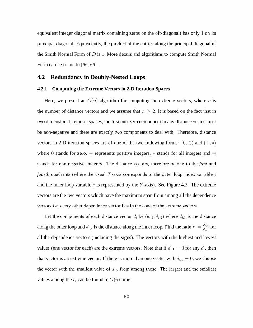
equivalent integer diagonal matrix containing zeros on the off-diagonal) has only1 on its
principal diagonal. Equivalently, the product of the entries along the principal diagonal of
the Smith Normal Form ofD is 1. More details and algorithms to compute Smith Normal
Form can be found in [56, 65].
4.2 Redundancy in Doubly-Nested Loops
4.2.1 Computing the Extreme Vectors in 2-D Iteration Spaces
Here, we present anO(n) algorithm for computing the extreme vectors, wheren is
the number of distance vectors and we assume thatn ≥ 2. It is based on the fact that in
two dimensional iteration spaces, the first non-zero component in any distance vector must
be non-negative and there are exactly two components to deal with. Therefore, distance
vectors in2-D iteration spaces are of one of the two following forms:(0,⊕) and(+, ∗)where0 stands for zero,+ represents positive integers,∗ stands for all integers and⊕
stands for non-negative integers. The distance vectors, therefore belong to thefirst and
fourth quadrants (where the usualX-axis corresponds to the outer loop index variablei
and the inner loop variablej is represented by theY -axis). See Figure 4.3. The extreme
vectors are the two vectors which have the maximum span from among all the dependence
vectorsi.e. every other dependence vector lies in the cone of the extreme vectors.
Let the components of each distance vectordi be (di,1, di,2) wheredi,1 is the distance
along the outer loop anddi,2 is the distance along the inner loop. Find the ratiori =di,2di,1
for
all the dependence vectors (including the signs). The vectors with the highest and lowest
values (one vector for each) are the extreme vectors. Note that ifdi,1 = 0 for anydi, then
that vector is an extreme vector. If there is more than one vector withdi,1 = 0, we choose
the vector with the smallest value ofdi,2 from among those. The largest and the smallest
values among theri can be found inO(n) time.
50
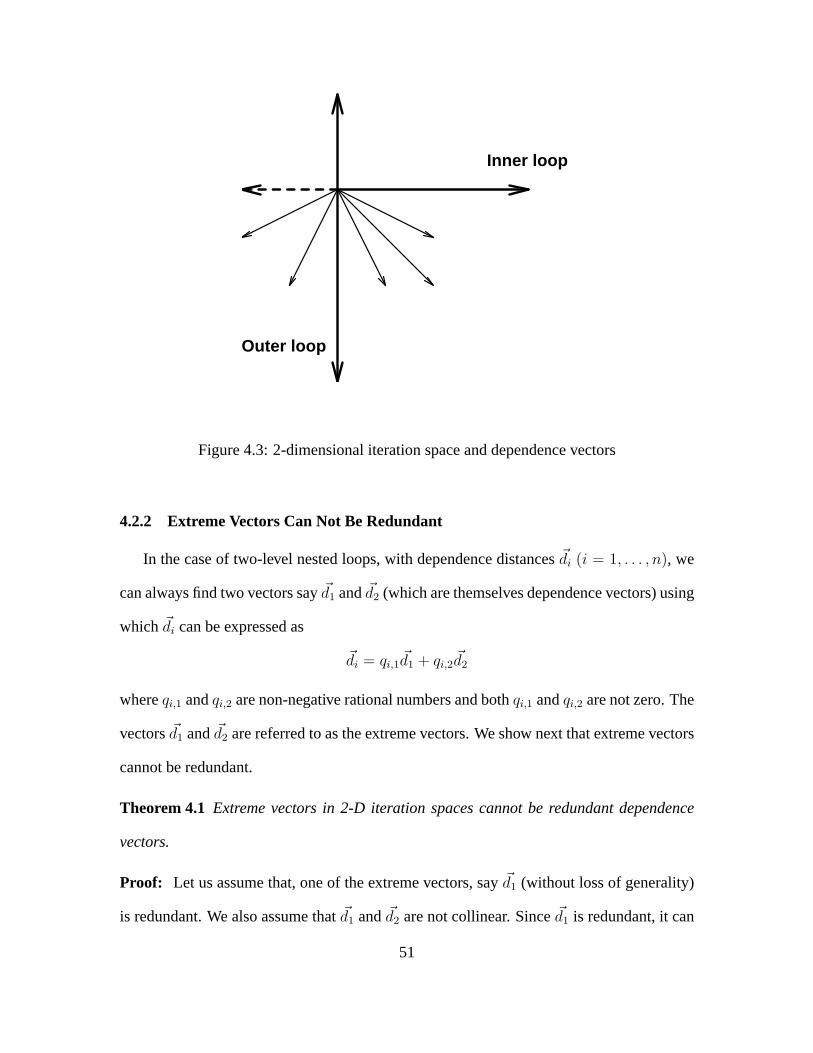
Outer loop
Inner loop
Figure 4.3: 2-dimensional iteration space and dependence vectors
4.2.2 Extreme Vectors Can Not Be Redundant
In the case of two-level nested loops, with dependence distances~di (i = 1, . . . , n), we
can always find two vectors say~d1 and~d2 (which are themselves dependence vectors) using
which ~di can be expressed as
~di = qi,1 ~d1 + qi,2 ~d2
whereqi,1 andqi,2 are non-negative rational numbers and bothqi,1 andqi,2 are not zero. The
vectors~d1 and~d2 are referred to as the extreme vectors. We show next that extreme vectors
cannot be redundant.
Theorem 4.1 Extreme vectors in 2-D iteration spaces cannot be redundant dependence
vectors.
Proof: Let us assume that, one of the extreme vectors, say~d1 (without loss of generality)
is redundant. We also assume that~d1 and ~d2 are not collinear. Since~d1 is redundant, it can
51
be expressed as a nonnegative linear combination of say~d2 and some dependence vector
~dk, (i.e.)
~d1 = α~d2 + β ~dk
whereα andβ are greater than zero. We assume that none of the vectors~dk is a scalar
multiple of either~d1 or ~d2. Since~dk is not an extreme vector,
~dk = ak,1 ~d1 + ak,2 ~d2
whereak,1, ak,2 > 0.
Therefore, it follows that
~d1 = α~d2 + β(ak,1 ~d1 + ak,2 ~d2
)
Since~d1 and ~d2 are not collinear
βak,1 = 1
and
α + βak,2 = 0 =⇒ α = −βak,2.
Sinceα, β, ak,i are all non-negative this is not possible, resulting in a contradiction.¤
LetE refer to the matrix whose columns are the extreme vectors~d1 and~d2. If the matrix
E is unimodular, then all dependences are redundant,i.e.,all the dependences (~d3 thru ~dn)
can be written in the form:
~di = ai,1 ~d1 + ai,2 ~d2
whereai,1 andai,2 are non-negative integers both not zero, (i.e.) all dependence vectors
have a non-negative integral decomposition on~d1 and ~d2; in other words~d1 and ~d2 form a
basis for a lattice [65]. A geometric interpretation for this is that, if you draw a parallelo-
gram at the origin(0, 0) of integer space whose sides are~d1 and ~d2, there will be no points
52
in the integer space belonging to the interior of this parallelogram (note that the interior
excludes the points~0, ~d1, ~d2 and~d1 + ~d2); the interior excludes the vertices but not the sides
of the parallelogram.
We have so far assumed that we do not have multiple dependence vectors along the
extreme vector directions. If this is the case, it suffices to enforce only the vector along that
direction, thegcd of whose components is 1. We have assumed that the iteration space is
connected. This is equivalent to assuming the iteration space dependence graph is weakly
connected, i.e., the undirected graph that results from omitting directions on dependence
edges is a connected graph. This constraint is satisfied if the dependence matrixD is g-
unimodular;if the matrixE is not unimodular, then it is not sufficient to enforce only the
extreme vectors. Essentially, we need to enforce additional dependences to synchronize
those integer vectors in the interior of the parallelogram generated by the extreme vectors
~d1 and ~d2. For example, consider a parallelogram whose sides are(2,−1) and(0, 1). The
vector(1, 0) lies inside this parallelogram. It is easy to see that the vector(1, 0) can not
be written as a non-negative integral linear combinations of(2,−1) and(0, 1). Also, the
matrix whose columns are(2,−1) and(0, 1) has a determinant of 2.
All the previous discussion ignored the size of the iteration space, or essentially as-
sumed a semi-infinite iteration space where a redundant dependence is redundant every-
where in the iteration space. This need not be true in finite iteration spaces [39], which is
the common case encountered.
4.2.3 Effect of the Size and Shape of the Iteration Space
Consider a two-level nested loop of the form:
for i1 = 0 to n− 1 do
53
for i2 = e ∗ i1 + x to f ∗ i1 + y do· · ·
endforendfor
wheren, e, x, f andy are constants. We also assume thatfi1 + y ≥ ei1 + x for all values
of i1, i.e.,0 ≤ i1 ≤ n− 1. Essentially, the inner loop limits are affine functions of the outer
loop variable. Let~I = (i1, i2) and ~J = (j1, j2) be two points in the iteration space, such
that ~I ≺ ~J, i.e., ~I executes before~J and ~J − ~I = ~d, for some dependence vector~d. We
say that the dependence vector~d exists at~I. Let the dependence vector~d be redundant,i.e.,
~d = ~a+~b where~a and~b are also dependence vectors.
We now present the conditions under which~d = (d1, d2) may not be redundant at~I,
i.e., cannot be enforced by~a and~b at ~I. This is possible when both~I and ~J = ~I + ~d
belong to the iteration space and neither~I+~a nor ~I+~b belong to the iteration space. Since
~I = (i1, i2) belongs to the iteration space
0 ≤ i1 (4.1)
i1 ≤ n− 1 (4.2)
ei1 + x ≤ i2 (4.3)
i2 ≤ fi1 + y (4.4)
Since~J = ~I + ~d = (i1 + d1, i2 + d2) belongs to the iteration space,
0 ≤ i1 + d1 (4.5)
i1 + d1 ≤ n− 1 (4.6)
e(i1 + d1) + x ≤ i2 + d2 (4.7)
i2 + d2 ≤ f(i1 + d1) + y (4.8)
54
Since~I + ~a does not belong to the iteration space,at least one of the following 4
conditions must be true:
0 > i1 + a1 (4.9)
i1 + a1 > n− 1 (4.10)
e(i1 + a1) + x > i2 + a2 (4.11)
i2 + a2 > f(i1 + a1) + y (4.12)
Similarly since~I +~b does not belong to the iteration space,at least one of the following
4 conditions should hold:
0 > i1 + b1 (4.13)
i1 + b1 > n− 1 (4.14)
e(i1 + b1) + x > i2 + b2 (4.15)
i2 + b2 > f(i1 + b1) + y (4.16)
Lemma 4.1 Conditions4.9, 4.10, 4.13 and4.14 can not be true.
Proof: Every dependence vector is apositive vector[8], i.e., the first nonzero component
of a dependence vector has to be positive. Therefore,a1 ≥ 0, b1 ≥ 0, d1 ≥ 0. Since
d1 = a1 + b1, and since(i1, i2) and(i1 + d1, i2 + d2) = (i1 + a1 + b1, i2 + a2 + b2) belong
to the iteration space, it follows that conditions4.9, 4.10, 4.13 and4.14 cannot be true.¤
For ~d not to be redundanti.e., non-redundantat ~I, at least one of the two conditions
4.11 and4.12 must hold and at least one of the two conditions4.15 and4.16 must hold.
We will consider the possibility of each of the four combinations, namely 4.11 and
4.15, 4.11 and 4.16, 4.12 and 4.15, and 4.12 and 4.16. Before that we derive some useful
additional results.
55

Result 4.1 If condition 4.11 is true, thenea1 > a2.
If condition 4.11 is true,
e(i1 + a1) + x > i2 + a2 =⇒ e(i1 + a1) + x ≥ i2 + a2 + 1
Condition 4.3 states
ei1 + x ≤ i2 or i2 ≥ ei1 + x
Adding these two, and canceling out common terms on the left and right sides, we have
ea1 ≥ a2 + 1 =⇒ ea1 > a2
If a1 6= 0, e > a2
a1.
Result 4.2 If condition 4.12 is true, thena2 > fa1.
If condition 12 is true,
i2 + a2 > f(i1 + a1) + y =⇒ i2 + a2 ≥ f(i1 + a1) + y + 1
Condition 4.4 states
fi1 + y ≥ i2
Adding these two, and canceling out common terms on the left and right sides, we have
a2 ≥ fa1 + 1 =⇒ a2 > fa1.
If a1 6= 0, a2
a1> f .
Result 4.3 If condition 4.15 is true, theneb1 > b2.
The derivation of this result is similar to the derivation of Result 4.1. For sake of brevity,
we omit details here. Ifb1 6= 0, e > b2b1
.
56
Result 4.4 If condition 4.16 is true, thenb2 > fb1.
The derivation of this result is similar to the derivation of Result 4.2. For sake of brevity,
we omit details here. Ifb1 6= 0, b2b1> f .
Lemma 4.2 Conditions 4.11 and 4.15 cannot both be true simultaneously.
Proof: Assume that conditions 4.11 and 4.15 are true simultaneously. Therefore results
4.1 and 4.3 hold,i.e.,
ea1 > a2 and eb1 > b2
=⇒ e(a1 + b1) > (a2 + b2) =⇒ ed1 > d2
Conditions 4.3 and 4.7 are:
ei1 + x ≤ i2
e(i1 + a1 + b1) + x ≤ i2 + a2 + b2
From these two, we can derive
e(a1 + b1) ≤ a2 + b2 =⇒ ed1 ≤ d2
which is a contradiction. ¤
Lemma 4.3 Conditions 4.12 and 4.16 can not both be true simultaneously.
Proof: The proof is similar to that of the previous lemma. ¤
As, a result, the only combinations left are: conditions 4.11 and 4.16, conditions 4.12
and 4.15. These combinations are symmetric. Therefore, we show the results only for one
of these combinations, 4.11 and 4.16.
57

Theorem 4.2 A dependence~d = ~a + ~b is not redundant at a point~I = (i1, i2) in an
arbitrary convex two dimensional iteration space if
(fi1 + y)− (ei1 + x) + 1 < (b2 − fb1) + (ea1 − a2) .
Proof: Conditions 4.11 and 4.16 are:
e(i1 + a1) + x > i2 + a2 =⇒ e(i1 + a1) + x ≥ i2 + a2 + 1
i2 + b2 > f(i1 + b1) + y =⇒ i2 + b2 ≥ f(i1 + b1) + y + 1
Adding these we get,
(b2 − a2) ≥ ((fi1 + y)− (ei1 + x) + 1) + (fb1 − ea1) + 1 =⇒
(b2 − a2) > ((fi1 + y)− (ei1 + x) + 1) + (fb1 − ea1)
where(fi1 +y)− (ei1 +x)+1 is sizeof the iteration space along the inner loop for a given
value of the outer loop index. Therefore, the dependence is not redundant if
size < (b2 − a2)− (fb1 − ea1) or,
size < (b2 − fb1) + (ea1 − a2)
The two quantities on the right hand side of the inequality are both positive. ¤
Corollary 4.1 A dependence~d = ~a +~b is not uniformly redundant at a point~I = (i1, i2)
in a rectangular two dimensional iteration space if the size of the iteration space along the
innermost loops satisfies the condition:
size < (b2 − a2)
whereb2 > 0 anda2 < 0.
58
Proof: For a rectangular iteration spacee = f = 0 andsize = y − x + 1. Substituting
these values in the result in theorem 4.2, we get
b2 − a2 ≥ (y − x+ 1) + 1 =⇒ b2 − a2 > (y − x+ 1).
Substituting these values in results 4.1 and 4.4 (from conditions 4.11 and 4.16), we also get
b2 > 0 anda2 < 0. Therefore, for the dependence to be non-redundant, the iteration space
along the innermost loop must be smaller than(b2 − a2) whereb2 > 0 anda2 < 0. ¤
This result is the same as that of [39].
4.2.4 Non-Constant Distance Vectors
Techniques presented in [39, 52] assume that the dependence vectors are distance vec-
tors (constant distance vectors). With non-constant distance vectors, we use the dependence
cone of the set of dependence vectors or the extreme vectors defined earlier. Thus, we need
to enforce only a fixed number of synchronizations per point in the iteration space. In some
cases, we need use extreme vectors which are not dependence vectors themselves resulting
in a loss of parallelism.
4.2.5 Non-Redundancy with Several Distance Vectors in 2-D
Let a dependence~r be redundant through a set of dependences~d1, . . . , ~dm, i.e.,
~r = ~d1 + ~d2 + · · ·+ ~dm
We assume that~r cannot be written as a non negative integral linear combination of a strict
subset of the vectors{~d1, ~d2, · · · , ~dm
}.
Assume a loop of the form:
for i1 = 0 to n1 − 1 dofor i2 = 0 to n2 − 1 do
59

· · ·endfor
endfor
Let ~I = (i1, i2) and ~J = (j1, j2) = (i1 + r1, i2 + r2) be points in the iteration space.
We approximate the non-redundancy relation as one where, for each dependence~dk (for
k = 1, · · · ,m wheredk,2 6= 0), the point(i1 + dk,1, i2 + dk,2) is not in the iteration space.
For each dependence at least one of the 4 conditions hold:
0 > i1 + dk,1 (R.1)
i1 + dk,1 > n1 − 1 (R.2)
0 > i2 + dk,2 (R.3)
i2 + dk,2 > n2 − 1 (R.4)
Using reasoning similar to that in Section 4.2.3, none of the conditions(R.1) and(R.2)
can not be true for allk = 1, · · · ,m. It is also not possible that all the conditions(R.3) are
true for allk if the dependence is to be non-redundant at some point; the same holds for all
(R.4).
For dependence to be non-redundant, some proper subset of the conditions(R.3) and
some proper subset of the conditions(R.4) should be true. Consider the subset of(R.3)
which are true; for all thesek,
i2 + dk,2 < 0
Since(i1, i2) belongs to the iteration space,
i2 ≥ 0
60

Combining these two, we getdk,2 < 0. Let max−(2) be the maximum among all these
dk,2. We have
i2 +max−(2) < 0 (4.17)
=⇒ i2 + dk,2 < 0 for all members of that set.
Similarly, consider the subset of(R.4) which are true; for all these k,
i2 + dk,2 > n2 − 1 or dk,2 > 0
Letmin+(2) be the minimum among all these. Letsize = n2. We have
i2 +min+(2) > n2 − 1 (4.18)
=⇒ i2 + dk,2 > n2 − 1 for all members of that set.
Combining the inequalities (4.17) and (4.18) we get,
max−(2) + i2 ≤ −1
n2 − 1 ≤ i2 +min+(2)− 1
=⇒ n2 − 1 ≤ min+(2)−max−(2)− 2
=⇒ n2 − 1 + 1 ≤ min+(2)−max−(2)− 1
=⇒ size < min+(2)−max−(2) (4.19)
This is a much stronger sufficient condition for the multiple dependence vector case than
the one presented in [39].
For a dependence to be uniformly redundant,
size ≥ min+(2)−max−(2)
61

or
size ≥ min+(2) +∣∣max−(2)
∣∣ .
In addition to this, thesize of the iteration space along the innermost loop must be large
enough for all the dependences~d1, . . . , ~dm to occur. Therefore, for a dependence to be
uniformly redundant, the following condition must hold:
size ≥ max{(min+(2) +
∣∣max−(2)∣∣) , (max+(2) + 1
),(∣∣min−(2)
∣∣+ 1)}
(4.20)
The result is illustrated through the following example. Consider a2-nested loop with
distance vectors(0, 3), (1,−2), (1,−1) and(2, 0). The distance vector(2, 0) is redundant
since it is the sum of the first three vectors. While, the result from this chapter, shows that
(2, 0) is uniformly redundant if the size of the inner loop is≥ 4, the result from [39] would
require that inner loop size be≥ 5. In addition, our results are applicable for arbitrary
shapes of the iteration space, while [39] works only for rectangular iteration spaces. See
Figure 4.4.
4.3 Redundancy in K-D (K > 2) Iteration Spaces
4.3.1 Computing the Extreme Vectors in K-D Iteration Spaces
In the case of higher dimensional iteration spaces, a subset of the dependence vectors
need not themselves be the extreme vectors. This is illustrated through the following ex-
ample:
Example 4.3:for i = 2 toN
for j = 2 toNfor k = 2 toN − 1A[i, j, k]← A[i− 1, j, k] + A[i, j − 1, k] + A[i, j, k − 1] + A[i− 1, j − 1, k + 1]
62

(2,0) is redundant everywhere in the iteration space
i
j
Figure 4.4: Illustration of redundancy with multiple distance vectors.
The loop has4 distance vectorsd1 = (1, 0, 0), d2 = (0, 1, 0), d3 = (0, 0, 1) andd4 =
(1, 1,−1). For any choice of three of the distance vectors as the extreme vector, the fourth
vector cannot be expressed as a non-negative linear combination of the three vectorsi.e.,
the fourth does not lie in the positive hull of the other three. In this case, the extreme vector
set consists of the following vectors(0, 0, 1), (1, 0,−1) and(0, 1, 0) of which only two are
dependence (distance) vectors.
In order to derive extreme vectors inK-D iteration spaces, we refer to the following
discussion on the equivalence of tiling planes [29, 61] and extreme vectors. Based on
results in [61], it follows that the problem of finding the tiling planes can be formulated as
63
(a linear programming problem) that of finding a transformationH such that
K∑
k=1
Hi,kDk,j ≥ 0 i = 1, . . . , K j = 1, . . . , n
with the constraint that
Hi,k = 0 if k > i
The rows ofH are the normals to the tiling planes and the columns ofH−1 are the spanning
(extreme) vectors. (Recall that the dependence vectors are expressed as non-negative linear
combinations of extreme vectors.) There may be an infinite number of sets of spanning
extreme vectors. With respect to scheduling, we are interested in theminimal set of extreme
vectors.A set of extreme vectors is minimal if it does not contain another set of spanning
extreme vectors. Finding the minimal set of extreme vectors is related to minimizing the
sum of the entriesK∑i=1
n∑j=1
K∑
k=1
Hi,kDk,j.
Thus the problem of finding the minimal set of extreme vectors reduces to the following
linear programming problem: FindH such that
K∑i=1
n∑j=1
K∑
k=1
Hi,kDk,j
is minimized subject to the constraints that
K∑
k=1
Hi,kDk,j ≥ 0 i = 1, . . . , K j = 1, . . . , n
Hi,k = 0 if k > i
Hi,k = 1 if k = i
Once we findH, we invertH. Given the restrictions we have used,H is unimodular;
thereforeH−1 is also unimodular. SinceH−1 is unimodular, all dependences other than
extreme vectors are redundant.
64

4.3.2 On Redundancy in Rectangular K-D Iteration Spaces
In K-nested loops, only the first component of the dependence vectors have to be non-
negative; there are no such constraints on the remaining components as long as the vector
is positive[8]. The discussion on non-uniformity of redundancy in two-level nested loops
(from the previous section) apply directly as long as along only one loop nest, we have
mixed distances,i.e., for at most one value ofi (2 ≤ i ≤ K), di,j (j = 1, . . . ,m where
m is the number of dependences) have negative and positive values. If dependences at a
level are either all non-negative or all non-positive, then redundancy is uniform.If there are
mixed distances at exactly one level, then the size of the iteration space along that nest level
must be large enough.If all the components at the same level in all the distance vectors
have the same sign, then redundancy is uniform in K-D iteration spaces,i.e., if di,j has the
same sign for allj = 1, . . . ,m for anyi(1 ≤ i ≤ K), then redundancy is uniform.
If there are mixed distances at more than one level, lack of redundancy is independent
of the size of the iteration space. There are always certain points in the iteration space,
where dependences are not redundant, even though at other points in the iteration space,
they may be redundant. This is independent of the size of the iteration space.
4.4 Chapter Summary
This chapter addressed the problem of eliminating redundant synchronization (and com-
munication) in the execution of nested loops on multiprocessors. The relatively high cost
of synchronization in these machines renders frequent synchronization very expensive. So,
it is of interest to enforce the minimum number of required synchronizations while preserv-
ing the parallelism in the computation. For two-level nested loops, we presented a method
to eliminate redundant dependences; our technique enforces the minimum number of the
required dependences. In nested loops, a dependence may be redundant in only a portion
65
of the iteration space. We characterized the non-uniformity of the redundancy of a depen-
dence in terms of the relation between the dependences and the shapes of the iteration space
and also in terms of the size of the iteration space in general convex 2-D iteration spaces.
In K-D (K ≥ 3) iteration spaces, we presented a method of determining the minimum re-
quired synchronizations by computing the minimal set of extreme vectors. We also discuss
the non-uniformity that arises for a specific class ofK-nested loops.
66
CHAPTER 5
GLOBAL TRANSFORMATIONS FOR LOCALITY
In order to achieve high levels of performance on parallel machines, it is essential to
reduce communication overhead and increase locality of reference. The data access times
on some shared memory multiprocessors neglecting the effects of caches is more or less
the same [36]. In contrast, on most multiprocessors (in particular, distributed-memory
message-passing machines), the access times to local data is significantly less than that
for non-local accesses [71]; such systems are referred to as Non-Uniform Memory Access
(NUMA) machines. On a NUMA machine, besides exploiting parallelism, one can in-
directly control the movement of data and thus the network traffic by specifying the task
distribution and scheduling.
Consider the KSR1 multiprocessor [71] which has no global shared memory; all data
movement is supported in hardware unlike distributed memory multiprocessors which use
software-controlled communication for non-local memory accesses. In order to improve
the performance on such machines, locality of reference should be exploited and commu-
nication overhead must be reduced. Most parallel programs consist possibly of a sequence
of loop nests that access common data arrays with similar access patterns. The programmer
has the choice of using pre-scheduling or self-scheduling algorithms for scheduling loop
iterations. Although self-scheduling results in proper load balancing, pre-scheduling, with
proper knowledge of the program semantics can result in good locality of reference [79].
The concept ofaffinity regionsas introduced by Appelbe and Lakshmanan [5], is defined
as a sequential set of loop nests that share the same schedule in the hope that this increases
67

data locality. The loop nest that is first scheduled and executed in a given affinity region
may be either pre-scheduled or self-scheduled and this schedule is then saved and later
used by loop nests present in the same affinity region. This scenario is especially useful in
optimizing accesses to locally stored data across loop nests in the same affinity region on a
multiprocessor. The KSR1 multiprocessor supports the concept of affinity based schedul-
ing by providing certain specifications and directives required in order to define affinity
regions [35]. The notion of affinity regions is useful for most NUMA machines. The key
issues involved in affinity-based scheduling that need to be addressed are:
• How do affinity regions perform in comparison to other alternatives such as loop
fusion and parallel regions?
• What transformations can be applied in conjunction with affinity regions that opti-
mize locality and parallelism?
This chapter presents a technique that determines the set of loop nests that can be placed in
an affinity region. In addition, we present an analytical approach that produces a compu-
tation decomposition which maps iterations in loops onto processors of a parallel machine
useful in preparing and maintaining schedules of iterations of different loop nests in the
same affinity region. Loop nests of the same as well as different depths have been consid-
ered. This approach finds loop transformations that can be applied to loops in the affinity
region resulting in a decomposition that tends to optimize locality in a given program with-
out sacrificing parallelism.
Section 5.1 discusses the background material and related work. In Section 5.2, the
actual techniques used are presented with examples. Section 5.3 examines more complex
cases involving more than one common data array in two loop nests belonging to the same
68
affinity region and illustrate the techniques using some examples. Finally, Section 5.4
concludes with a summary and discusses further avenues of research.
5.1 Background
The need to maintain data locality and reduce the communication overhead for achieving
high levels of performance on massively parallel machines has led to research that has
resulted in several approaches [5, 4]. As described earlier, an affinity region is a set of
loop nests that share the same schedule [5]. This concept of affinity region is described by
Example 5.1 below:
Example 5.1.
forall j = 1, N doforall i = 1, N do
S1: A (i, j) = 0for k = 1, N do
S2: A(i, j) = A(i, j) +B(k, i) ∗ C(k, j)endfor
endforendforforall i = 1, N do
for k = 1, N doS3: D(i) = D(i) +B(k, i)
endforendfor
In the above example, one can see that we have a common data array,B, that is accessed
both the loop nests. The objective here is to ensure data locality so that the two loop nests
share the same schedule. What needs to be determined is, which iterations in both the loop
nests should be allocated to the same processor so that locality of access to common data
is maintained; in addition, transformations (loop interchange, loop reversaletc.) that need
to be applied in one or both of the loop nests, are also to be determined.
69
Appelbe and Lakshmanan [5] have discussed other approaches to the problem of opti-
mizing locality of reference across two loops by ensuring that they share the same sched-
ule. Besides using the concept of affinity regions,loop fusion[75, 79] andparallel regions
[5, 79] can also be used in increasing data locality across loops having common shared
arrays; of course, all dependencies are preserved as well. In Example 5.1 we can see that
no more transformations are needed to place the two loops in an affinity region since loop
interchange has already been applied to the first loop. Let us now look at the approach of
using loop fusion to the same above program (Example 5.1) and see how beneficial this
method is. As mentioned by Zima and Chapman [79], two adjacent loops can be fused
together to form one loop if there are no loop carried dependencies between them.
As we can see in Example 5.1, there are no loop carried dependencies in both loops
[5]. The arrayB is accessed by columns in both cases and there are no dependencies from
statementsS2 to S3 or vice versa. Now the question arises as to whether any changes
be need to be made in either or both the loops in order to fuse them together? From the
structure of both loops, it is obvious that loop with indexj has to be made the inner most
loop in the first loop nest. Since the loop with indexj is now the inner loop, the initialization
of arrayA in the first loop nest (statementS1) cannot be placed anywhere else since it has
to be placed after loop with indexj but before the loop with indexk. Thus the initialization
of arrayA has now to be moved out [5] and placed outside the first loop nest as shown in
Example 5.2 below:
Example 5.2
for i = 1, N doforall j = 1, N do
S1: A(i, j) = 0endfor
endfor
70

for i = 1, N dofor k = 1, N do
forall j = 1, N doS2: A(i, j) = A(i, j) + B(k, i) ∗ C(k, j)
endforS3: D(i) = D(i) + B(k, i)
endforendfor
From the above program we see that the objective of using loop fusion has not been
achieved, since it has created another nest for initializing the arrayA. Furthermore, data
locality is reduced after fusion; and the problem of reduced locality can be solved only if
the loop with indexj is serialized and arraysA andC ’s subscripts are interchanged [5].
Can these transformations be performed on the fused version in Example 5.2? It is not
possible to change subscripts in the above example and thus we see that fusion of loops in
this case has created more problems than providing a solution.
In using parallel regions, the part of the code that is enclosed in the region is exe-
cuted in parallel on all processors except cases where one processor has to wait for another
when they synchronize on loop iterations [79]. Parallel regions have been found to be not
beneficial since mapping iterations to processors requires usage of parameters that the pro-
grammer has to use while specifying parallel regions [5]. Appelbe and Lakshmanan [5]
also noted that even though the programmer has specified directives in defining parallel
regions and has also mapped the iterations to processors, sometimes the same iteration is
executed on some other processor not defined by the user due to automatic load balancing.
If this happens, the locality of reference is lost and the communication overhead increases.
Affinity regions [5] are another approach to this problem and in using this method
we have the ability to specify the set of loop nests that should share the same processor
schedules. What we find by this approach is the set of iterations in each of the loop nests
71
that access the same elements of the array accessed. This can be found only if the loop
nests have some common accesses to a particular data array. Once the set of iterations
in each loop is found and the required transformations applied, it is then the job of the
compiler to determine a suitable scheduling strategy to execute the iterations. The choice
of the scheduling strategy is left to the compiler and not to the programmer, unlike parallel
regions where the programmer has to specify the scheduling [5]. Some languages such as
the KSR Parallel Fortran [33, 34] (used by Appelbe and Lakshmanan [5] in their study of
affinity regions), include specific directives that are used to define affinity regions and tile
sizes of the iteration space. But the loops that have been defined in the affinity region must
have the same loop indices and their loop bounds must either be the same or should be
overlapping.
5.1.1 Related Work
Appelbe and Lakshmanan [5] presented an algorithm based on affinity regions with
the goal of accessing same elements of the shared array by the same processor across
loop nests belonging to the same region. Their techniques examines which loops can be
included in the same affinity region and under what conditions are they included. Appelbe
and Lakshmanan [5] have stated that the loops being considered have to be parallelizable
at some level of the nesting. They have also considered only cases where exists only one
shared array across the loop nests. One of the key issues involved in having more than one
shared array across the loops is as to which of the shared arrays is thedominantone of the
shared arrays. What would happen if there are two shared arrays and the nesting level is
the same in both loops in one case and different in the other? This chapter addresses these
issues and approaches the problem of mapping iterations involving single shared arrays in
a mathematical framework which produces the required transformations that need to be
72
applied to one or both the loops in order to schedule the iterations that involve accesses to
the same element of the common data array onto the same processor.
A mathematical approach has been presented by Anderson and Lam [4] that tries to
optimize data locality and parallelism. They developed a compiler algorithm based on pri-
marily three components, namely, partitioning, orientation and displacement that together
specify mapping of data and loop iterations to processors. The compiler algorithm [4] first
normalizes the loops and applies loop distribution. The decomposition algorithms [3] are
then applied before the compiler performs a loop fusion over the program to fuse compati-
ble loop nests [21, 79]. They consider parallel loops and their work is not aimed at affinity
scheduling.
A number of researchers have addressed this issue of iteration decomposition among
processors to improve locality of reference by reducing communication. Algorithms for in-
creasing parallelism and locality inside a single loop nest have been developed [36, 43, 72].
Some researchers have also looked at the problem of mapping iterations and corresponding
data accessed in a single loop nest onto parallel machines [27, 40, 41]. Several of them have
developed data decomposition algorithms through a fixed performs an exhaustive search of
all possible decompositions to produce a static data decomposition with least communi-
cation [24]. In contrast, the approach used in this chapter does not perform exhaustive
searches and is able to derive a computation decomposition of loop iterations of nested
loops belonging to a given affinity region. This chapter has also taken into consideration
multiple shared arrays across loop nests of equal and varied depths. It also looks at the
possibility of deriving an iteration decomposition that satisfies locality constraints for all
shared arrays involved, failing which it presents an approach to find the dominant array
among all the shared arrays being considered.
73
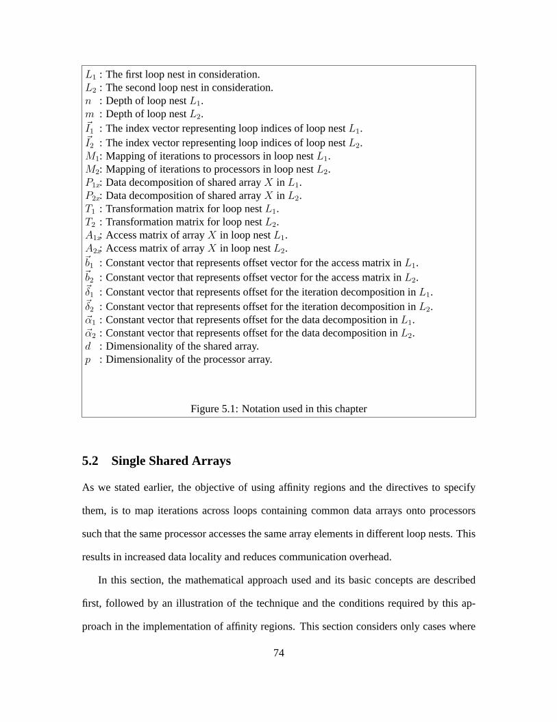
L1 : The first loop nest in consideration.L2 : The second loop nest in consideration.n : Depth of loop nestL1.m : Depth of loop nestL2.~I1 : The index vector representing loop indices of loop nestL1.~I2 : The index vector representing loop indices of loop nestL2.M1: Mapping of iterations to processors in loop nestL1.M2: Mapping of iterations to processors in loop nestL2.P1x: Data decomposition of shared arrayX in L1.P2x: Data decomposition of shared arrayX in L2.T1 : Transformation matrix for loop nestL1.T2 : Transformation matrix for loop nestL2.A1x: Access matrix of arrayX in loop nestL1.A2x: Access matrix of arrayX in loop nestL2.~b1 : Constant vector that represents offset vector for the access matrix inL1.~b2 : Constant vector that represents offset vector for the access matrix inL2.~δ1 : Constant vector that represents offset for the iteration decomposition inL1.~δ2 : Constant vector that represents offset for the iteration decomposition inL2.~α1 : Constant vector that represents offset for the data decomposition inL1.~α2 : Constant vector that represents offset for the data decomposition inL2.d : Dimensionality of the shared array.p : Dimensionality of the processor array.
Figure 5.1: Notation used in this chapter
5.2 Single Shared Arrays
As we stated earlier, the objective of using affinity regions and the directives to specify
them, is to map iterations across loops containing common data arrays onto processors
such that the same processor accesses the same array elements in different loop nests. This
results in increased data locality and reduces communication overhead.
In this section, the mathematical approach used and its basic concepts are described
first, followed by an illustration of the technique and the conditions required by this ap-
proach in the implementation of affinity regions. This section considers only cases where
74

there is one common data array across loop nests. Loop nests with the same as well as
different nesting levels have also been considered in this section.
5.2.1 Basic Concepts
Let us consider the case of two adjacent loop nests that are to be placed in an affin-
ity region. The notation and symbols used in this mathematical approach are shown in
Figure 5.1.
Definition 5.1 [4]
The data decomposition of ad-dimensional array,X, onto ap-dimensional processor array
for each access index~x is a function defined byP(~x) as:
P(~x) = P~x+ ~α (5.1)
whereP is ap×d dimensional matrix,~α is the constant offset vector and~x represents each
element in the array,~x = (x1, ...,xd).
Definition 5.2 [4]
The iteration decomposition of the loop nest onto ap-dimensional processor array for each
iteration~i in the loop nest of depthn is defined by the functionC(~i) as:
C(~i) = M~i+ ~δ (5.2)
whereM is ap× n transformation matrix,~δ is a constant offset vector and~i = (i1, ..., in).
From Definition 5.1, one can say that for two elements~x1 and ~x2 to be allocated to the
same processor whenP represents the data decomposition, the following condition must
hold:
P ~x1 = P ~x2 =⇒ P ( ~x1 − ~x2) = ~0. (5.3)
Similarly, from Definition 5.2, it can be said that two iterations~i1 and~i2 are scheduled on
the same processor for execution withM as the iteration decomposition matrix if and only
75
if,
M~i1 = M~i2 =⇒M(~i1 − ~i2) = ~0. (5.4)
In order to relate the iteration and data decompositions, both the iterations and the data el-
ements that they access must be allocated to the same processor. This ensures data locality.
Definition 5.3
For all iterations~I in loop nestL1, array elements and iterations that reference these ele-
ments will be local to a processor if and only if,
M1~I1 + ~δ1 = P1x(A1x
~I1 + ~b1) + ~α1 (5.5)
If we do not consider any offsets, the above equation becomes
M1~I1 = P1xA1x
~I1 (5.6)
Thus in order to maximize data locality, one has to find a decompositionP and an iteration
mappingM and hence reduce communication. In the following subsection, we present
the conditions under which loops can be placed in an affinity region. Loops that satisfy
the criteria are placed in the affinity region and are calledaffinity adjacent loops. Data
transfers arising from offsets degrades performance to a limited extent [4]; for the rest of
this chapter, we will omit offsets in deriving the necessary relations.
5.2.2 Criteria for Affinity Adjacent Loops
The approach presented in this chapter first decide which loop nests can be placed in
an affinity region; this decision is made subject to several conditions. The goal of placing
loop nests in an affinity region is to improve locality and this is done by deriving a suitable
computation decomposition. If such a decomposition is found then iterations in the first
loop nest can be scheduled by the compiler using any strategy and the schedule is then
76

saved and used by the second loop nest in the affinity region. Our approach is based on the
following assumptions:
(1) At each level in both loop nests, the subscripts of every array variable accessed should
be an affine function of the loop indices in the corresponding loop nests.
(2) All the loops involved are for loops or forall loops; loops at any nesting level must have
a fixed lower bound, upper bound and stride.
The conditions to be satisfied for loops to be placed in the affinity region are:
A. There should exist a dependence from a shared array in loop nestL1 to same array
in loop nestL2 and the subscripts of the shared array in both loop nests must be
functions of the loop indices.
B. The loop indices in the loop nestsL1 andL2 must be the same; in addition, the loop
bounds of corresponding loop indices must be the same or overlapping.
C. There should be no accesses to the shared array in the intervening code (if any) between
the two loop nests.
Once the above three conditions are satisfied, we perform the following analysis. As seen
from Definition 5.3, for iterations and data accessed by these iterations involving the shared
arrayX, to be allocated to the same processor, we have the following equation for loop nest
L1:
M1~I1 + ~δ1 = P1x(A1x
~I1 + ~b1) + ~α1. (5.7)
Similarly for loop nestL2, we have,
M2~I2 + ~δ2 = P2x(A2x
~I2 + ~b2) + ~α2. (5.8)
77

Since we are not considering offsets, the above equations are reduced to the following: In
loop nestL1,
M1~I1 = P1xA1x
~I1, (5.9)
and in loop nestL2,
M2~I2 = P2xA2x
~I2. (5.10)
Now in both the loop nests,L1 andL2, there are accesses to the elements of the shared
arrayX. Since the goal is to form a decomposition of iterations so that the same schedule
is used by the next loop in the affinity region, the shared array should have the same data
decomposition across both loop nestsL1 andL2. Hence we can say that
P1x = P2x (5.11)
Using 5.11 in equations 5.9 and 5.10, we get
M1(A1x)−1 = M2(A2x)
−1, (5.12)
which can be written as:
M1(A1x(T1)−1)−1 = M2(A2x(T2)−1)−1, (5.13)
As seen in equation 5.13, access matricesA1x andA2x are known andM1 andM2 are
the unknowns.T1 andT2 represent the transformations to be applied to loop nestsL1 and
L2. The transformation matrix is a unit matrix when no transformation is applied to the
corresponding loop nest. There are two cases here which depend basically on the nesting
levels in loop nestsL1 andL2.
Case 1:n = m Here we consider the case where the level of nesting is the same in both
loop nests and hence the loop indices are the same as well. The loop bounds in both nests
78
are either the same or overlapping. Both the access matricesA1x andA2x have the same
dimension. To obtain a computation decomposition that preserves the locality of reference
equation 5.12 must be satisfied. Whenn = m, there are two possibilities.
(1)A1x = A2x
When the access matrices are the same, no transformations are required in either of the
loop nestsL1 orL2, and they can be placed in an affinity region as it is.
(2)A1x 6= A2x
When the access matrices are different we need to find a transformation that can be applied
to either or both loops such that equation 5.12 is satisfied. Basically the transformations
when applied to either or both the loop nests produces access matrices in both nests for the
shared arrayX, such thatA1x = A2x.
Case 2:n 6= m Here we consider the case where the level of nesting is different in both
the loop nests. Eithern > m or n < m. The loop indices of the loop nest with a smaller
nesting level must be a subset of the loop indices of the loop nest which has the higher level
of nesting. The loop bounds associated with the corresponding loop indices must be the
same or overlapping. Lets consider the case ofn > m. The following analysis is going to
be the same forn < m. Sincen > m, A1x is ad × n matrix andA2x is ad ×m matrix.
A transformation needs to be found and this can be done by changing access matrices in
either or both access matrices such that a column subset of the transformed matrixA1x of
dimensiond × m, is equal toA2x or the transformedA2x. The chosen column subset of
matrixA1x must contain contiguous columns of the matrixA1x. The all zero columns of
the matrixA1x that are not part of the chosen column subset must be pushed to form the
79
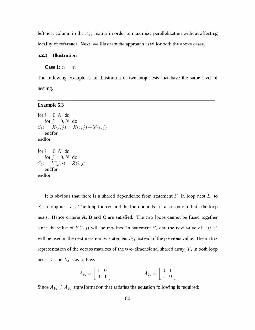
leftmost column in theA1x matrix in order to maximize parallelization without affecting
locality of reference. Next, we illustrate the approach used for both the above cases.
5.2.3 Illustration
Case 1:n = m
The following example is an illustration of two loop nests that have the same level of
nesting.
Example 5.3
for i = 0, N dofor j = 0, N do
S1: X(i, j) = X(i, j) + Y (i, j)endfor
endfor
for i = 0, N dofor j = 0, N do
S2: Y (j, i) = Z(i, j)endfor
endfor
It is obvious that there is a shared dependence from statementS1 in loop nestL1 to
S2 in loop nestL2. The loop indices and the loop bounds are also same in both the loop
nests. Hence criteriaA, B andC are satisfied. The two loops cannot be fused together
since the value ofY (i, j) will be modified in statementS2 and the new value ofY (i, j)
will be used in the next iteration by statementS1, instead of the previous value. The matrix
representation of the access matrices of the two-dimensional shared array,Y , in both loop
nestsL1 andL2 is as follows:
A1y =
[1 00 1
]A2y =
[0 11 0
]
SinceA1y 6= A2y, transformation that satisfies the equation following is required:
80
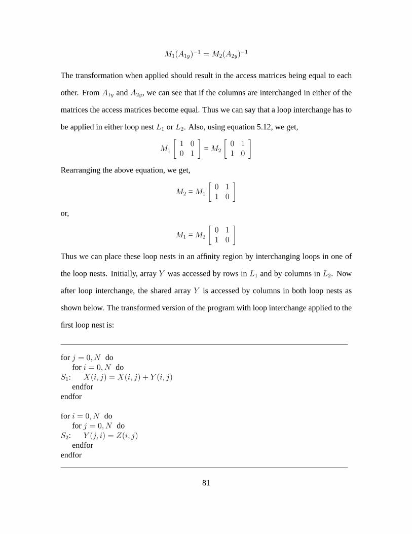
M1(A1y)−1 = M2(A2y)
−1
The transformation when applied should result in the access matrices being equal to each
other. FromA1y andA2y, we can see that if the columns are interchanged in either of the
matrices the access matrices become equal. Thus we can say that a loop interchange has to
be applied in either loop nestL1 orL2. Also, using equation 5.12, we get,
M1
[1 00 1
]= M2
[0 11 0
]
Rearranging the above equation, we get,
M2 = M1
[0 11 0
]
or,
M1 = M2
[0 11 0
]
Thus we can place these loop nests in an affinity region by interchanging loops in one of
the loop nests. Initially, arrayY was accessed by rows inL1 and by columns inL2. Now
after loop interchange, the shared arrayY is accessed by columns in both loop nests as
shown below. The transformed version of the program with loop interchange applied to the
first loop nest is:
for j = 0, N dofor i = 0, N do
S1: X(i, j) = X(i, j) + Y (i, j)endfor
endfor
for i = 0, N dofor j = 0, N do
S2: Y (j, i) = Z(i, j)endfor
endfor
81

Had the transformation been applied to loop nestL2, the elements of the arrayY , would
be then accessed by rows. Using the KSR directives, we can define the iteration tile space
asj : 0, i : N for loop nestL1 andi : 0, j : N for loop nestL2.
Case 2:n 6= m
This is an example of the case where both loop nests have different levels of nesting
and the example that has been presented hasn > m.
Example 5.4
for i = 1, N dofor j = 1, N do
S1: A (i, j) = 0for k = 1, N do
S2: A(i, j) = A(i, j) + B(k, i) ∗ C(k, j)endfor
endforendforfor i = 1, N do
for k = 1, N doS3: D(i) = D(i) + B(k, i)
endforendfor
As it has been stated earlier the above program cannot be fused into one loop as loop
j in nestL1 will have to be moved to the innermost and so the initialization of arrayA in
statementS1 will have to be moved out. In effect, the above two loops will produce two
loop nests even after fusion, one of them performing the initializing of arrayA as inS1.
In Example 5.4 presented above, loop nestL1 has a nesting level of three (n = 3) and
loop nestL2 has a nesting level of two (m = 2). Loop indices used in loopL2, i andk, are
a subset of loop indices,i, j andk, used in loop nestL1. The bounds are same for all loop
indices and there exists a shared array dependence from loop nestS2 in L1 toS3 in L2. The
access matrices in every iteration for the arrayB in L1 andL2 is given by,
82
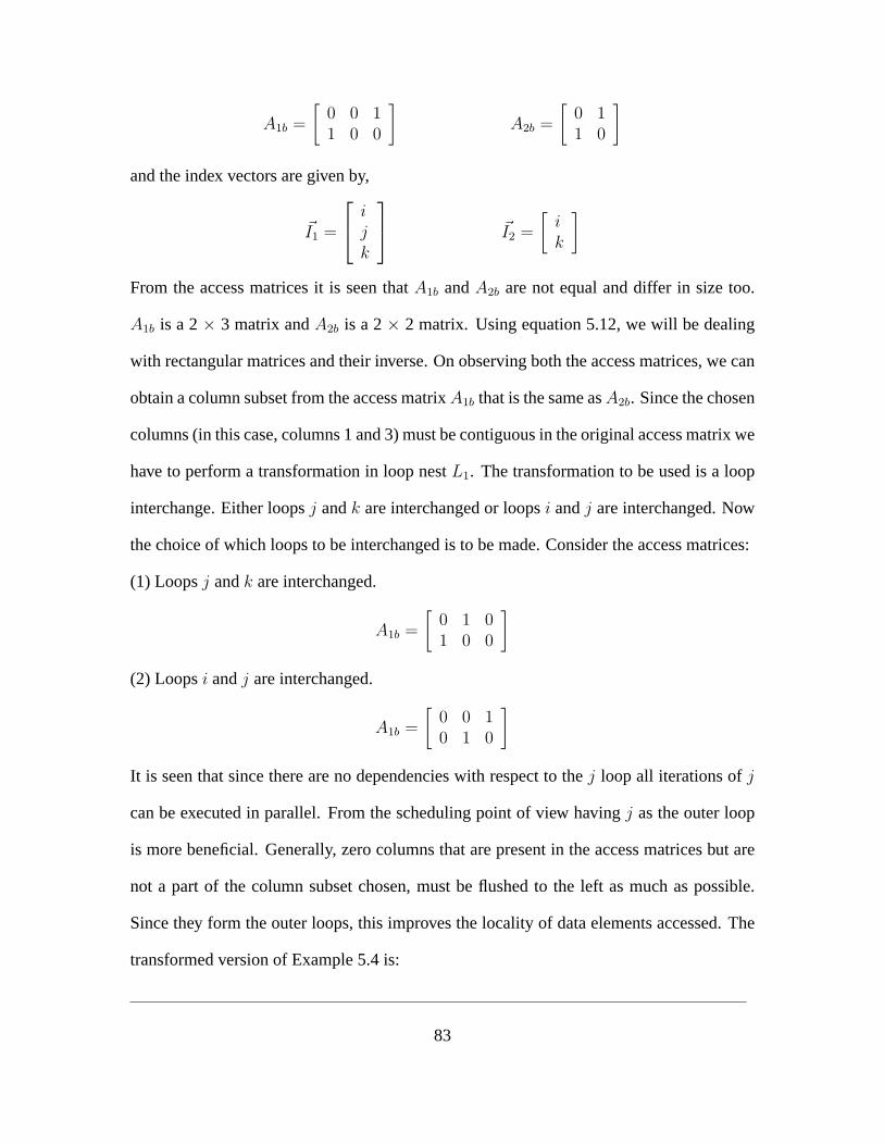
A1b =
[0 0 11 0 0
]A2b =
[0 11 0
]
and the index vectors are given by,
~I1 =
ijk
~I2 =
[ik
]
From the access matrices it is seen thatA1b andA2b are not equal and differ in size too.
A1b is a 2× 3 matrix andA2b is a 2× 2 matrix. Using equation 5.12, we will be dealing
with rectangular matrices and their inverse. On observing both the access matrices, we can
obtain a column subset from the access matrixA1b that is the same asA2b. Since the chosen
columns (in this case, columns 1 and 3) must be contiguous in the original access matrix we
have to perform a transformation in loop nestL1. The transformation to be used is a loop
interchange. Either loopsj andk are interchanged or loopsi andj are interchanged. Now
the choice of which loops to be interchanged is to be made. Consider the access matrices:
(1) Loopsj andk are interchanged.
A1b =
[0 1 01 0 0
]
(2) Loopsi andj are interchanged.
A1b =
[0 0 10 1 0
]
It is seen that since there are no dependencies with respect to thej loop all iterations ofj
can be executed in parallel. From the scheduling point of view havingj as the outer loop
is more beneficial. Generally, zero columns that are present in the access matrices but are
not a part of the column subset chosen, must be flushed to the left as much as possible.
Since they form the outer loops, this improves the locality of data elements accessed. The
transformed version of Example 5.4 is:
83
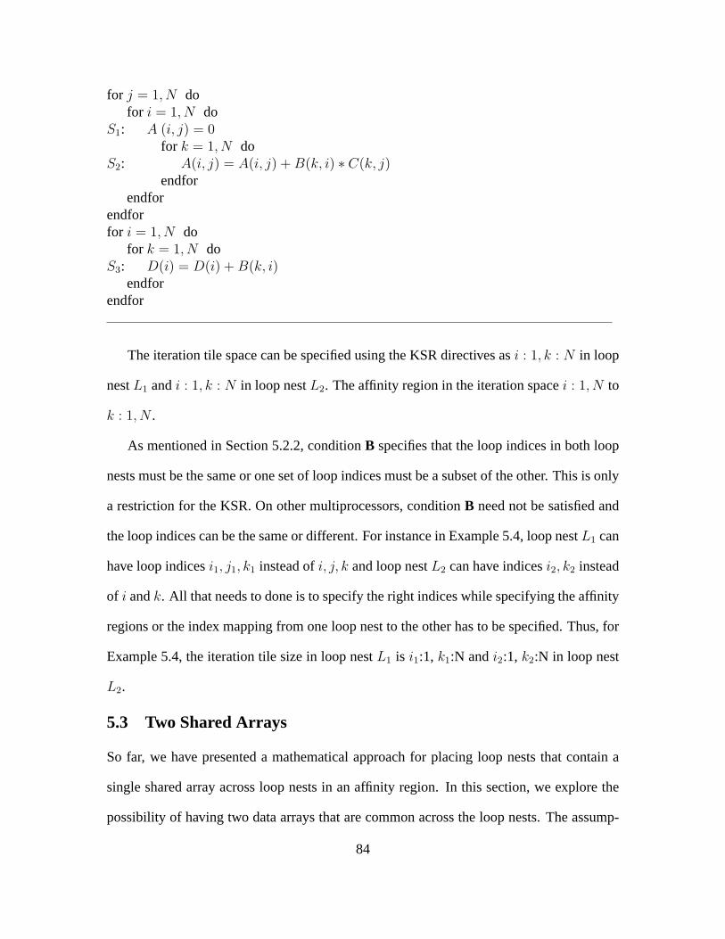
for j = 1, N dofor i = 1, N do
S1: A (i, j) = 0for k = 1, N do
S2: A(i, j) = A(i, j) + B(k, i) ∗ C(k, j)endfor
endforendforfor i = 1, N do
for k = 1, N doS3: D(i) = D(i) + B(k, i)
endforendfor
The iteration tile space can be specified using the KSR directives asi : 1, k : N in loop
nestL1 andi : 1, k : N in loop nestL2. The affinity region in the iteration spacei : 1, N to
k : 1, N .
As mentioned in Section 5.2.2, conditionB specifies that the loop indices in both loop
nests must be the same or one set of loop indices must be a subset of the other. This is only
a restriction for the KSR. On other multiprocessors, conditionB need not be satisfied and
the loop indices can be the same or different. For instance in Example 5.4, loop nestL1 can
have loop indicesi1, j1, k1 instead ofi, j, k and loop nestL2 can have indicesi2, k2 instead
of i andk. All that needs to done is to specify the right indices while specifying the affinity
regions or the index mapping from one loop nest to the other has to be specified. Thus, for
Example 5.4, the iteration tile size in loop nestL1 is i1:1, k1:N andi2:1, k2:N in loop nest
L2.
5.3 Two Shared Arrays
So far, we have presented a mathematical approach for placing loop nests that contain a
single shared array across loop nests in an affinity region. In this section, we explore the
possibility of having two data arrays that are common across the loop nests. The assump-
84
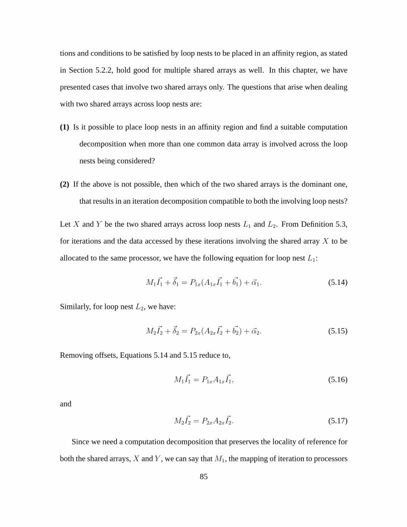
tions and conditions to be satisfied by loop nests to be placed in an affinity region, as stated
in Section 5.2.2, hold good for multiple shared arrays as well. In this chapter, we have
presented cases that involve two shared arrays only. The questions that arise when dealing
with two shared arrays across loop nests are:
(1) Is it possible to place loop nests in an affinity region and find a suitable computation
decomposition when more than one common data array is involved across the loop
nests being considered?
(2) If the above is not possible, then which of the two shared arrays is the dominant one,
that results in an iteration decomposition compatible to both the involving loop nests?
Let X andY be the two shared arrays across loop nestsL1 andL2. From Definition 5.3,
for iterations and the data accessed by these iterations involving the shared arrayX to be
allocated to the same processor, we have the following equation for loop nestL1:
M1~I1 + ~δ1 = P1x(A1x
~I1 + ~b1) + ~α1. (5.14)
Similarly, for loop nestL2, we have:
M2~I2 + ~δ2 = P2x(A2x
~I2 + ~b2) + ~α2. (5.15)
Removing offsets, Equations 5.14 and 5.15 reduce to,
M1~I1 = P1xA1x
~I1, (5.16)
and
M2~I2 = P2xA2x
~I2. (5.17)
Since we need a computation decomposition that preserves the locality of reference for
both the shared arrays,X andY , we can say thatM1, the mapping of iteration to processors
85
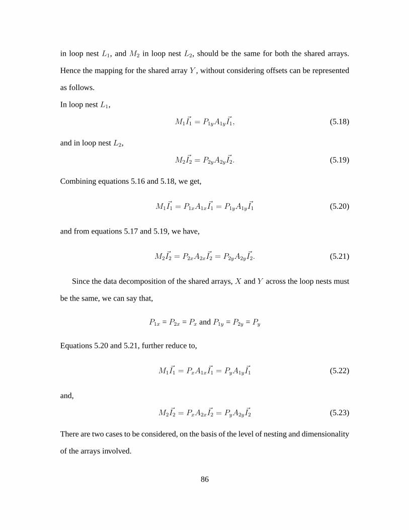
in loop nestL1, andM2 in loop nestL2, should be the same for both the shared arrays.
Hence the mapping for the shared arrayY , without considering offsets can be represented
as follows.
In loop nestL1,
M1~I1 = P1yA1y
~I1, (5.18)
and in loop nestL2,
M2~I2 = P2yA2y
~I2. (5.19)
Combining equations 5.16 and 5.18, we get,
M1~I1 = P1xA1x
~I1 = P1yA1y~I1 (5.20)
and from equations 5.17 and 5.19, we have,
M2~I2 = P2xA2x
~I2 = P2yA2y~I2. (5.21)
Since the data decomposition of the shared arrays,X andY across the loop nests must
be the same, we can say that,
P1x = P2x = Px andP1y = P2y = Py
Equations 5.20 and 5.21, further reduce to,
M1~I1 = PxA1x
~I1 = PyA1y~I1 (5.22)
and,
M2~I2 = PxA2x
~I2 = PyA2y~I2 (5.23)
There are two cases to be considered, on the basis of the level of nesting and dimensionality
of the arrays involved.
86
Case 1:n = m and d = n Here we consider that the nesting level is same in both the
loop nests involved and the shared arrays,X andY , have the same dimensiond, which
is equal to the level of nesting. IfA1x = A2x andA1y = A2y, then no transformations
are required and the loops can be placed in an affinity region as it is. Under any other
circumstance, some transformation is needed and we need to find a suitable mapping of
iteration to processors. Since the loop indices are the same in both the loop nests and the
level of nesting is also the same, we have,
~I1 = ~I2 = ~I (5.24)
From equations 5.22, 5.23 and 5.24, we have,
M2~I = M1(A1x)
−1A2x~I, (5.25)
and
M2~I = M1(A1y)
−1A2y~I (5.26)
The above equations lead to,
M1(A1x)−1A2x = M1(A1y)
−1A2y, (5.27)
or
M1
((A1x)
−1A2x − (A1y)−1A2y
)= ~0 (5.28)
Since the only variable isM1 in the above equation, we can find a suitable iteration decom-
position on to the processors such that communication is reduced and locality of reference
is increased.
Case 2: n = m and d 6= n When the nesting level is not the same asd (the dimen-
sionality of the array), it is difficult to use equation 5.28 since we would be dealing with
87
rectangular inverses. Thus out of the two shared arrays, the dominant array has to be found
which maintains the locality of the other shared array. An arrayX is said to be domi-
nant in comparison to another shared arrayY , if the iteration decomposition resulting from
the shared arrayX results in better locality for all references made to array elements in
the given loop nests. The access matrix of the dominant array is used in determining the
iteration decomposition necessary to specify the iteration tile size in each of the loop nests.
Let X andY be the two shared arrays. We know the access matricesA1x, A2x, A1y,
andA2y from the loop nestsL1 andL2. Consider the first shared array,X, and perform
transformations onL1 andL2 such thatA1x = A2x. Now upon removing the zero columns
from the access matricesA1y andA2y, if,
A1y = A2y
then the shared array,X, is the dominant array. If this is not the case, we should consider
the access matrix of arrayY , and perform the same analysis. If a dominant array cannot be
found, then it becomes the case of a single shared array, and either of the two shared arrays
can be used.
We have considered cases where the nesting levels in both loop nests are the same,i.e.,
n = m. Whenn 6= m, and the dimension of the shared arraysX andY is the same, the
same approach as described in Case 2 above can be used to determine the dominant array.
Additionally, ~I1 6= ~I2, but one of them is a subset of the other.
5.3.1 Illustration
The following example is a program that has the same nesting level in both loop nests
and both the shared arrays have the same dimension which is also equal to the nesting level.
Example 5.5
88
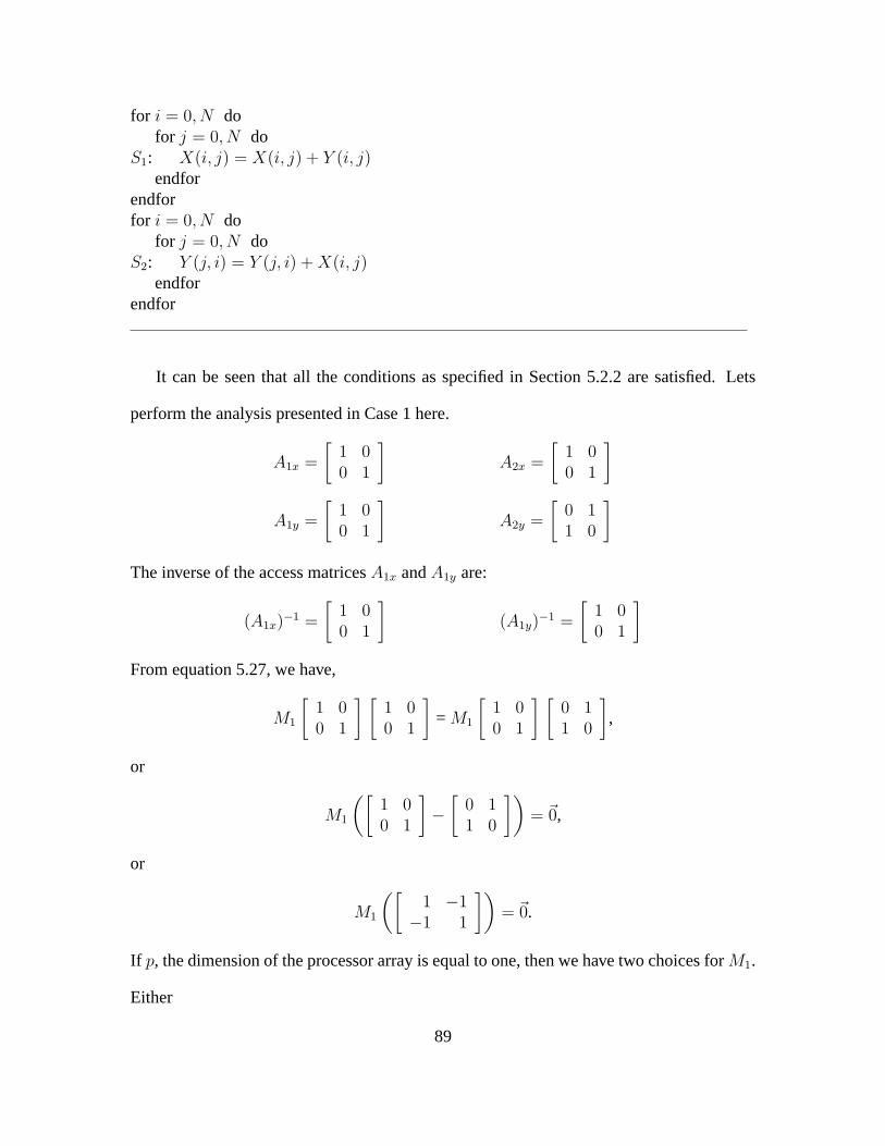
for i = 0, N dofor j = 0, N do
S1: X(i, j) = X(i, j) + Y (i, j)endfor
endforfor i = 0, N do
for j = 0, N doS2: Y (j, i) = Y (j, i) +X(i, j)
endforendfor
It can be seen that all the conditions as specified in Section 5.2.2 are satisfied. Lets
perform the analysis presented in Case 1 here.
A1x =
[1 00 1
]A2x =
[1 00 1
]
A1y =
[1 00 1
]A2y =
[0 11 0
]
The inverse of the access matricesA1x andA1y are:
(A1x)−1 =
[1 00 1
](A1y)
−1 =
[1 00 1
]
From equation 5.27, we have,
M1
[1 00 1
] [1 00 1
]= M1
[1 00 1
] [0 11 0
],
or
M1
([1 00 1
]−[
0 11 0
])= ~0,
or
M1
([1 −1−1 1
])= ~0.
If p, the dimension of the processor array is equal to one, then we have two choices forM1.
Either
89
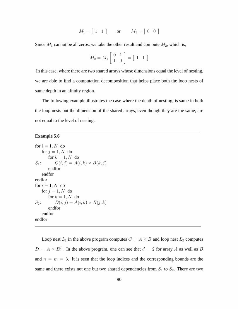
M1 =[
1 1]
or M1 =[
0 0]
SinceM1 cannot be all zeros, we take the other result and computeM2, which is,
M2 = M1
[0 11 0
]=[
1 1]
In this case, where there are two shared arrays whose dimensions equal the level of nesting,
we are able to find a computation decomposition that helps place both the loop nests of
same depth in an affinity region.
The following example illustrates the case where the depth of nesting, is same in both
the loop nests but the dimension of the shared arrays, even though they are the same, are
not equal to the level of nesting.
Example 5.6
for i = 1, N dofor j = 1, N do
for k = 1, N doS1: C(i, j) = A(i, k)×B(k, j)
endforendfor
endforfor i = 1, N do
for j = 1, N dofor k = 1, N do
S2: D(i, j) = A(i, k)×B(j, k)endfor
endforendfor
Loop nestL1 in the above program computesC = A × B and loop nestL2 computes
D = A × BT . In the above program, one can see thatd = 2 for arrayA as well asB
andn = m = 3. It is seen that the loop indices and the corresponding bounds are the
same and there exists not one but two shared dependencies fromS1 to S2. There are two
90

shared arrays and we need to find which one is the dominant one. Let us derive their access
matrices first.
A1a =
[1 0 00 0 1
]A2a =
[1 0 00 0 1
]
A1b =
[0 0 10 1 0
]A2b =
[0 1 00 0 1
]
Consider the access matrices of the shared arrayA. A transformation is required such that
a subset of contiguous columns from both access matricesA1a andA2a, are equal. In order
to do this let us interchange thej andi loops in both the loop nests. The access matrices
now become,
A1a =
[0 1 00 0 1
]A2a =
[0 1 00 0 1
]
A1b =
[0 0 11 0 0
]A2b =
[1 0 00 0 1
]
We have achieved the desired result for the shared arrayA. But removing the zero column
from the access matrices for arrayB results in a 2× 2 matrix; the two resulting matrices
are not equal. We can say that the locality of the arrayB is not preserved and hence, the
shared arrayA, cannot be the dominant array.
Let us consider the arrayB now. If we perform a loop interchange in loop nestL2 only
between thej loop and thek loop, the new access matrices are:
A1a =
[1 0 00 0 1
]A2a =
[1 0 00 1 0
]
A1b =
[0 0 10 1 0
]A2b =
[0 0 10 1 0
]
We have achieved the desired result for arrayB. Now if we remove the zero column
from the access matrices of arrayA, we see that the resultant 2× 2 matrices are equal.
91

Thus locality of arrayA is maintained. Thus the arrayA is accessed by rows even after
the interchange has been performed. SinceB is the dominant array we can specify both
the affinity region and the computation decomposition based on the shared arrayB. The
transformed version of the above program is as follows:
for i = 1, N dofor j = 1, N do
for k = 1, N doS1: C(i, j) = A(i, k)×B(k, j)
endforendfor
endforfor i = 1, N do
for k = 1, N dofor j = 1, N do
S2: D(i, j) = A(i, k)×B(j, k)endfor
endforendfor
The above illustration depicts a case where only one of the shared arrays is the dominant
array. The choice of the dominant array was easy in Example 5.6, since only arrayB was
the dominant one. In a situation where both the shared arrays are dominant, we can not
use the approach mentioned earlier in Case 2 of this section. Thus, the decision of which
dominant array is used in deriving transformations and defining affinity regions has to be
made. This is illustrated by the following example. Consider the following program:
Example 5.7
for i = 1, N dofor j = 1, N do
for k = 1, N doS1: C(i, j) = A(i, k)×B(k, j)
92
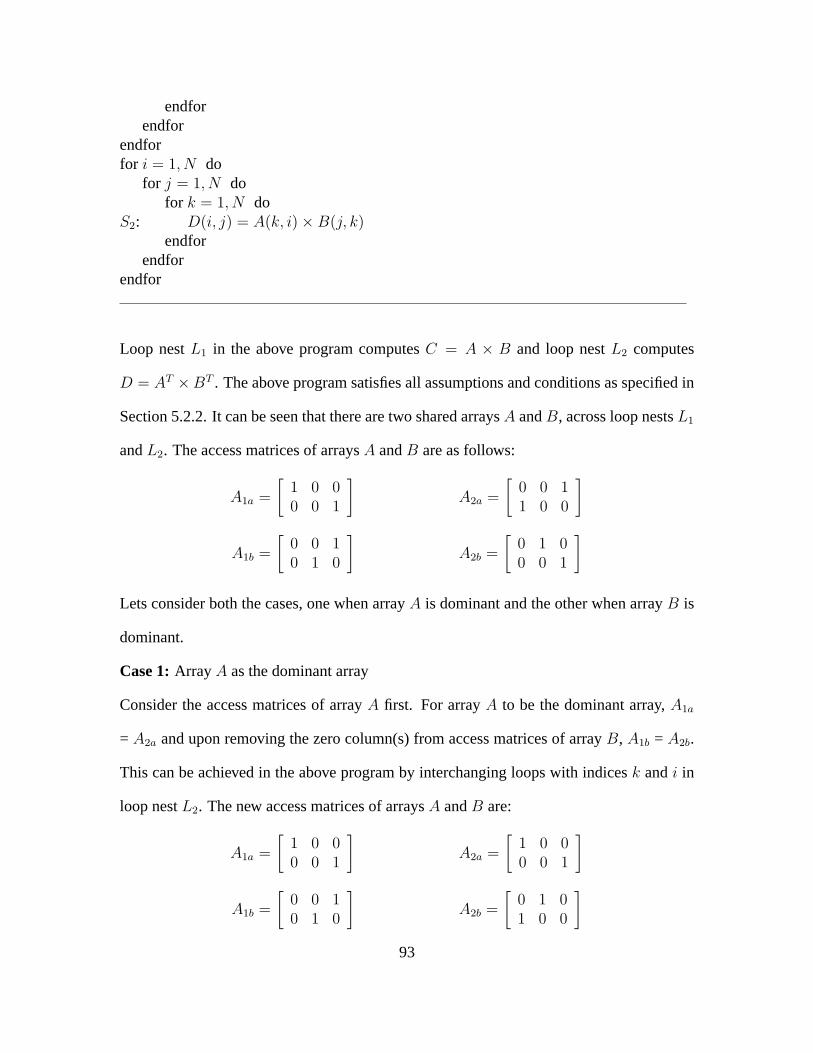
endforendfor
endforfor i = 1, N do
for j = 1, N dofor k = 1, N do
S2: D(i, j) = A(k, i)×B(j, k)endfor
endforendfor
Loop nestL1 in the above program computesC = A × B and loop nestL2 computes
D = AT ×BT . The above program satisfies all assumptions and conditions as specified in
Section 5.2.2. It can be seen that there are two shared arraysA andB, across loop nestsL1
andL2. The access matrices of arraysA andB are as follows:
A1a =
[1 0 00 0 1
]A2a =
[0 0 11 0 0
]
A1b =
[0 0 10 1 0
]A2b =
[0 1 00 0 1
]
Lets consider both the cases, one when arrayA is dominant and the other when arrayB is
dominant.
Case 1:ArrayA as the dominant array
Consider the access matrices of arrayA first. For arrayA to be the dominant array,A1a
= A2a and upon removing the zero column(s) from access matrices of arrayB, A1b = A2b.
This can be achieved in the above program by interchanging loops with indicesk andi in
loop nestL2. The new access matrices of arraysA andB are:
A1a =
[1 0 00 0 1
]A2a =
[1 0 00 0 1
]
A1b =
[0 0 10 1 0
]A2b =
[0 1 01 0 0
]
93
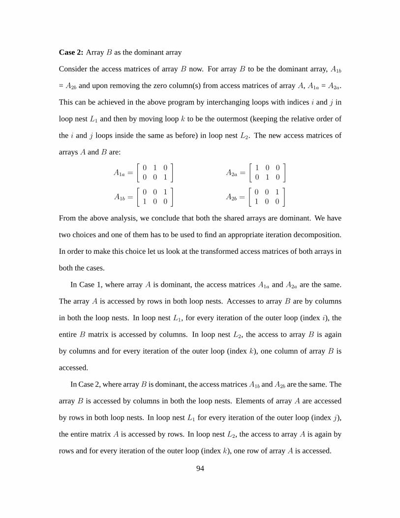
Case 2:ArrayB as the dominant array
Consider the access matrices of arrayB now. For arrayB to be the dominant array,A1b
= A2b and upon removing the zero column(s) from access matrices of arrayA, A1a = A2a.
This can be achieved in the above program by interchanging loops with indicesi andj in
loop nestL1 and then by moving loopk to be the outermost (keeping the relative order of
the i andj loops inside the same as before) in loop nestL2. The new access matrices of
arraysA andB are:
A1a =
[0 1 00 0 1
]A2a =
[1 0 00 1 0
]
A1b =
[0 0 11 0 0
]A2b =
[0 0 11 0 0
]
From the above analysis, we conclude that both the shared arrays are dominant. We have
two choices and one of them has to be used to find an appropriate iteration decomposition.
In order to make this choice let us look at the transformed access matrices of both arrays in
both the cases.
In Case 1, where arrayA is dominant, the access matricesA1a andA2a are the same.
The arrayA is accessed by rows in both loop nests. Accesses to arrayB are by columns
in both the loop nests. In loop nestL1, for every iteration of the outer loop (indexi), the
entireB matrix is accessed by columns. In loop nestL2, the access to arrayB is again
by columns and for every iteration of the outer loop (indexk), one column of arrayB is
accessed.
In Case 2, where arrayB is dominant, the access matricesA1b andA2b are the same. The
arrayB is accessed by columns in both the loop nests. Elements of arrayA are accessed
by rows in both loop nests. In loop nestL1 for every iteration of the outer loop (indexj),
the entire matrixA is accessed by rows. In loop nestL2, the access to arrayA is again by
rows and for every iteration of the outer loop (indexk), one row of arrayA is accessed.
94
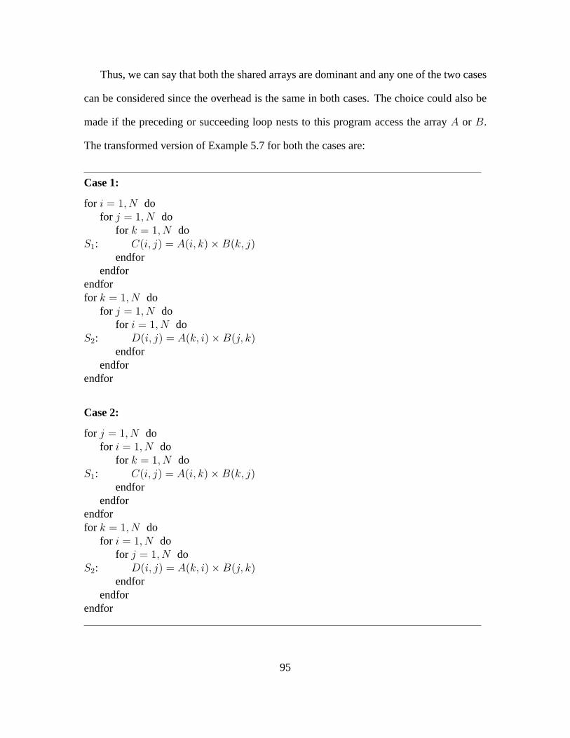
Thus, we can say that both the shared arrays are dominant and any one of the two cases
can be considered since the overhead is the same in both cases. The choice could also be
made if the preceding or succeeding loop nests to this program access the arrayA or B.
The transformed version of Example 5.7 for both the cases are:
Case 1:
for i = 1, N dofor j = 1, N do
for k = 1, N doS1: C(i, j) = A(i, k)×B(k, j)
endforendfor
endforfor k = 1, N do
for j = 1, N dofor i = 1, N do
S2: D(i, j) = A(k, i)×B(j, k)endfor
endforendfor
Case 2:
for j = 1, N dofor i = 1, N do
for k = 1, N doS1: C(i, j) = A(i, k)×B(k, j)
endforendfor
endforfor k = 1, N do
for i = 1, N dofor j = 1, N do
S2: D(i, j) = A(k, i)×B(j, k)endfor
endforendfor
95

5.3.2 Multiple Loop Nests
So far, only two loop nests have been used in all cases and discussions. In this sub-
section, we look at affinity regions involving more than two loop nests. To begin with,
consider Example 5.4 in Section 5.2.3. The program in that example has two loop nests
that have one common data array. The question that now arises is that if there was an outer
loop enclosing the two loop nests, can the loop nests be still placed in an affinity region
without any variations?
Let us enclose the two nested loops by an outer loop. The program that we consider is
shown in Example 5.8.
Example 5.8
for l = 1, N dofor j = 1, N do
for i = 1, N dofor k = 1, N do
S1: A(i, j) = A(i, j) +B(k, i)× C(k, j)endfor
endforendforfor i = 1, N do
for k = 1, N doS2: D(i) = D(i) +B(k, i)
endforendfor
endfor
The access matrices for the shared arrayB are:
A1b =
[0 0 0 10 0 1 0
]A2b =
[0 0 10 1 0
]
As can be seen from the access matrices, thel loop does not have any effect on the place-
ment of loop nests in an affinity region. Thus one can say that as long as a given set of
96
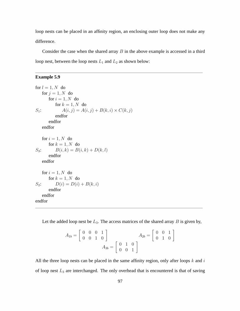
loop nests can be placed in an affinity region, an enclosing outer loop does not make any
difference.
Consider the case when the shared arrayB in the above example is accessed in a third
loop nest, between the loop nestsL1 andL2 as shown below:
Example 5.9
for l = 1, N dofor j = 1, N do
for i = 1, N dofor k = 1, N do
S1: A(i, j) = A(i, j) +B(k, i)× C(k, j)endfor
endforendfor
for i = 1, N dofor k = 1, N do
S3: B(i, k) = B(i, k) +D(k, l)endfor
endfor
for i = 1, N dofor k = 1, N do
S2: D(i) = D(i) +B(k, i)endfor
endforendfor
Let the added loop nest beL3. The access matrices of the shared arrayB is given by,
A1b =
[0 0 0 10 0 1 0
]A2b =
[0 0 10 1 0
]
A3b =
[0 1 00 0 1
]
All the three loop nests can be placed in the same affinity region, only after loopsk andi
of loop nestL3 are interchanged. The only overhead that is encountered is that of saving
97

the schedule. Thus, it is possible to place as many loop nests in the same affinity region as
long as they satisfy all the criteria stated earlier in this subsection and in Section 5.2.2.
Consider the case where there are four sequential loop nestsL1, L2, L3 andL4. Based
on the analysis presented so far in this chapter, if nestsL1 andL3 have a common data
arrayX, andL2 andL4 also have a common data arrayY , logically we should be able to
placeL1 andL3 in one affinity region andL2 andL4 in another affinity region. But since
Y , the shared array in loop nestL2 is different from the shared arrayX in loop nestsL1
andL3, locality of reference would be destroyed. Thus, it is preferable to place loop nest
L2 in the same affinity region asL1 andL3; as a result, it cannot be placed in any other
affinity region. Note that a loop nest can belong to only one affinity region.
5.4 Chapter Summary
This chapter has presented an approach using a mathematical framework for the problem
of placing loop nests that have one or more data arrays in common, in an affinity region.
As stated earlier, Appelbe and Lakshmanan [5] developed an algorithm for placing nests
in an affinity region. Their algorithm described in Section 5.1, takes into consideration
only cases where one shared array is involved. Anderson and Lam [4] have used a data
decomposition approach which is more like affinity data regions, whereas this chapter has
presented an approach based on affinity control regions.
We have found limitations in the usage of loop fusion and parallel regions. The ap-
proach used in this chapter is capable of handling more complex cases than single shared
arrays across loop nests. There need not necessarily be a parallel loop in the nests. This
chapter has also considered cases involving two shared arrays that extends easily to mul-
tiple shared arrays; in addition, we have presented different instances that depend on the
array dimensionality and the depth of nesting in the loop nests involved. Throughout this
98
chapter, in our approach, we have had to satisfy the criteria that the loop indices of the loop
nests involved must be the same or one set of loop indices must be a subset of the other.
This is a restriction only for the KSR1 multiprocessor and can be ignored when compiling
for other multiprocessors.
Thus, one can see that affinity regions are more effective than other approaches such
as loop fusion and parallel regions in deriving a computation decomposition that maintains
locality and reduces communication. The approach used in this chapter is more beneficial
as it has considered many instances not explored in previous work. Work is in progress on
the problem of deciding the best grouping of adjacent loop nests for affinity-based schedul-
ing, in which data rearrangement between adjacent groups is allowed. This requires good
cost models of data accesses and data reorganization. Some of this work bears similarity to
work currently in progress on automatic data distribution for distributed memory machines.
99
CHAPTER 6
CONCLUSIONS
Exploiting parallelism in loops in programs is an important factor in realizing the po-
tential performance of processors today. This work has developed and evaluated several
compiler optimizations aimed at improving the performance of loops on processors.
6.1 Address Code Optimization
An important class of problems used widely in scientific computing and other application
domains perform memory intensive computations on large data sets. An important feature
of the class of problems (called stencil problems) considered in Chapter 2 is the regularity
exhibited by their access patterns. In Chapter 2, we presented an approach of optimizing
the address generation of these stencil problems.
These code segments have two major overheads: (i) the pure arithmetic computation
overhead and (ii) the memory address computation overhead. These overheads determine
the performance of these code segments. Callahan et al. [9] propose an approach to op-
timize these stencil codes and thereby improve their performance. They replace all sub-
scripted array variables by scalars, thereby effecting reuse of these scalar variables. These
scalar variables are then mapped to registers. Subsequent reuse of these data elements
means that they can be directly accessed from registers instead of through the cache mech-
anism. This means that loads of all reused data elements can be serviced at processor speed
instead of having to deal with cache conflicts and subsequent loads from secondary mem-
ory. This approach results in a good improvement in performance because the memory
address computation overhead has been reduced. However the major disadvantage with
100

this approach is that because of the large number of data elements that might be reused, the
number of scalars that will be needed is also large. This creates a lot of register pressure
which then starts to degrade performance. Also this approach does not seek to reduce the
pure arithmetic computation overhead.
We have presented an approach to optimize stencil codes with a view of reducing both
the arithmetic and the address computation overhead. The regularity of the access pattern
and the reuse of data elements between successive iterations of the loop body means that
there is a common sub-expression between any two successive iterations. If we were to
store the value of the common sub-expression in a scalar, then for the successive iteration,
the value in this scalar could be used instead of performing the computation all over again.
This greatly reduces the arithmetic overhead. Since we store only one scalar in a register,
there is almost no register pressure. Also all array accesses are now replaced by pointer
dereferences. This reduces the address computation overhead. These optimizations helped
to improve the performance of the stencil codes to a large extent. We also compared the
performance with some other popular approaches. The results in Section 2.3 demonstrate
conclusively that our approach is better than the one proposed by Callahan et al. [9].
Future work could include integrating the effects of induction variable analysis and op-
timization, as well as in reducing storage overhead in non-stencil codes, and in combining
these with data layout optimization techniques.
6.2 Fine-Grain Scheduling
Software pipelining is an effective fine-grain scheduling technique that restructures the
statements in the body of a loop subject to resource and dependence constraints such that
one iteration of a loop can start execution before another finishes. The total execution time
of a software-pipelined loop depends on the interval between two successive initiation of
101
iterations. While software pipelining of single loops has been addressed in many papers,
little work has been done in the area of software pipelining of nested loops.
In Chapter 3, we have presented an approach to software pipelining of nested loops.
We formulated the problem of finding the minimum iteration initiation interval for each
level of a nested loop as one of finding a rational affine schedule for each statement in the
body of a perfectly nested loop; this is then solved using linear programming. This frame-
work allows for an integrated treatment of iteration-dependent statement reordering and
multidimensional loop unrolling. Unlike most work in scheduling nested loops, we treat
each statement in the body as a unit of scheduling. Thus, the schedules derived allow for
instances of statements from different iterations to be scheduled at the same time. Optimal
schedules derived here subsume extant work on software pipelining of non-nested loops.
Possible avenues for further work includes deriving near-optimal multidimensional
loop unwinding in the presence of resource constraints and conditionals.
6.3 Redundant Synchronization
In order to achieve maximal parallel execution, a program must be decomposed into as
many concurrent tasks as possible. The dependences in the original program must be
preserved in concurrent execution to guarantee correctness, often through the use of syn-
chronization instructions. Synchronization involves large overhead such as busy-waiting,
contention for shared access or message passing. Therefore, it is important to minimize
the number of synchronization instructions while guaranteeing correct and (possibly) max-
imally parallel execution.
Chapter 4 addressed the problem of elimination of redundant synchronizations in paral-
lel execution of nested loops. The synchronization due to a dependence is redundant if it is
enforced by synchronizations due to other dependences or by a combination of a collection
102

of dependences and the control structure of the target machine. For two-level nested loops,
we have presented a method to eliminate redundant dependences; our technique enforces
the minimum number of the required dependences. In nested loops, a dependence may be
redundant in only a portion of the iteration space. We characterized the non-uniformity of
the redundancy of a dependence in terms of the relation between the dependences and the
shapes of the iteration space and also in terms of the size of the iteration space in general
convex2-D iteration spaces. For K-D(K ≥ 3) iteration spaces, we presented a method
of determining the minimum required synchronizations by computing the minimal set of
extreme vectors. We also discussed the non-uniformity that arises for a specific class of
K-nested loops.
Evaluating the tradeoff between synchronization overhead and loss of parallelism re-
quires future work. Also, further work is required for the problem of detecting redundant
synchronization in convex iteration spaces of dimension≥ 3.
6.4 Global Transformations for Exploiting Locality
In order to increase performance levels of a parallel machine, communication overhead
has to be reduced along with increasing data locality. The access times to local data is
usually much less than that for non-local accesses. If the elements frequently accessed by
iterations in a given loop nest are local to the processor on which the iterations are executed,
then communication overhead is greatly reduced. Moreover, if the same data elements are
being accessed by iterations in the following loop nests, the communication overhead is
minimized by scheduling iterations accessing the same elements in different loop nests to
the same processor. Chapter 5 presented a mathematical approach using the concept of
affinity regions to find a transformation such that a suitable iteration-to-processor mapping
can be found across a sequence of loop nests having the same shared arrays. This not only
103
improves the data locality but significantly reduces communication overhead. Since the
concept of affinity regions is being used, the schedule of the first loop nest in the affinity
region is saved and used by other nests in the affinity region. The iterations of the first
loop nest can be scheduled by the compiler and the only overhead involved is in saving this
schedule for subsequent loop nests in the affinity region.
Appelbe and Lakshmanan [5] developed an algorithm for placing nests in an affin-
ity region. Their algorithm described in Section 5.1, takes into consideration only cases
where one shared array is involved. Anderson and Lam [4] have used a data decomposi-
tion approach which is more like affinity data regions, whereas our work has presented an
approach based on affinity control regions.
We have found limitations in the usage of loop fusion and parallel regions. The ap-
proach used in Chapter 5 is capable of handling more complex cases than single shared
arrays across loop nests. There need not necessarily be a parallel loop in the nests. Chap-
ter 5 has also considered cases involving two shared arrays that extends easily to multiple
shared arrays; in addition, we have presented different instances that depend on the array
dimensionality and the depth of nesting in the loop nests involved. Throughout Chapter 5,
in our approach, we have had to satisfy the criteria that the loop indices of the loop nests
involved must be the same or one set of loop indices must be a subset of the other. This is a
restriction only for the KSR1 multiprocessor and can be ignored when compiling for other
multiprocessors.
Thus, one can see that affinity regions are more effective than other approaches such
as loop fusion and parallel regions in deriving a computation decomposition that main-
tains locality and reduces communication. The approach used in the fifth chapter is more
beneficial as it has considered many instances not explored in previous work.
104
Further work is required in developing an estimate as to how useful affinity regions are
and more work needs to be done when there are multiple shared arrays across loop nests.
In addition, work needs to be done in deciding the best grouping of adjacent loop nests for
affinity-based scheduling, which allows data rearrangement between adjacent groups. This
requires good cost models of data accesses and data reorganization.
105
BIBLIOGRAPHY
[1] A. Aiken. Compaction based parallelization. (Ph.D. thesis).Technical Report 88-922,Cornell University, 1988.
[2] A. Aiken and A. Nicolau. Optimal loop parallelization. InProc. ACM SIGPLANConference on Programming Languages Design and Implementation,June 1988.
[3] R. Allen and K. Kennedy. Automatic translation of FORTRAN programs to vectorform. ACM Trans. Programming Languages and Systems,9(4):491–542, 1987.
[4] Jennifer M. Anderson and Monica S. Lam. Global Optimizations for Parallelism andLocality on Scalable Parallel Machines.Proceedings of SIGPLAN’93, Conferenceon Programming Language Design and Implementation (PLDI),Albuquerque, NewMexico, June 23-25, 1993.
[5] B. Appelbe and B. Lakshmanan. Optimizing Parallel Programs using Affinity Re-gions.Tech. Rep. GIT-ICS-92/59, Georgia Institute of Technology, Nov. 1992.
[6] A. Bachem. The Theorem of Minkowski for Polyhedral Monoids and AggregatedLinear Diophantine Systems.Optimization and Operations Research – Proc. of Work-shop,University of Bonn, October 1977, Lecture Notes in Economics and Mathemat-ical Systems, Vol. 157, pages 1–14, Springer Verlag.
[7] D. Bacon, S. Graham, and O. Sharp. Compiler Transformations for High-PerformanceComputing.ACM Computing Surveys,Vol. 26, No. 4, pages 345-420, December1994.
[8] U. Banerjee.Dependence analysis for supercomputing,Kluwer Academic Publishers,Boston, MA, 1988.
[9] D. Callahan, S. Carr and K. Kennedy. Improving Register Allocation for SubscriptedVariables. InProc. ACM SIGPLAN ’90 conference on Programming Language Designand Implementation,1990.
[10] A. Carle, K. Kennedy, U. Kremer and J. Mellor-Crummey. Automatic Data Layoutfor Distributed-Memory Machines in the D Programming Environment.TechnicalReportCRPC TR93-298, Rice University, February 1993.
[11] F. Catthoor, S. Wuytack, E. De Greef, F. Balasa, L. Nachtergaele, A. Vandecappelle.Custom Memory Management Methodology,Kluwer Academic Publishers, 1998.
106
[12] R. Cytron. Compile-time scheduling and optimization for asynchronous machines.PhD thesis, University of Illinois at Urbana-Champaign, Urbana, Illinois, 1984.
[13] R. Cytron. DOACROSS: Beyond vectorization for multiprocessors.Proc. 1986 Inter-national Conference on Parallel Processing,pp. 836-844, August 1986.
[14] K. Danckaert, F. Catthoor, and H. De Man. System-level memory management forweakly connected image processing. InProc. Euro-Par’96, 1996.
[15] K. Ebcioglu. A compilation technique for fine-grain scheduling of loops with con-ditional jumps. InProc. 20th Annual Workshop on Microprogramming,December1987.
[16] P. Feautrier. Array expansion. InInternational Conference on Supercomputing,pages429-442, 1988.
[17] J. Fisher. Trace scheduling: A technique for global microcode compaction.IEEETrans. Comput., C-30(7):478–490, July 1971.
[18] J. Fisher. Very long instruction word architectures and the ELI-512. InProc. 10thInternational Symposium on Computer Architecture,pp. 140–150, June 1983.
[19] G. Gao, Y. Wong, and Q. Ning. A Petri-Net model for fine-grain loop scheduling.In Proc. ACM SIGPLAN Conf. Programming Language Design and Implementation,pp. 204-218, Toronto, Canada, June 1991.
[20] G. Gao, Q. Ning and V. van Dongen. Extending fine-grain scheduling for schedulingnested loops. InProc. 6th Annual Workshop on Languages and Compilers for ParallelComputing,August 1993.
[21] G. R. Gao, R. Olsen, V. Sarkar and R. Thekkath. Collective Loop Fusion for ArrayContraction. Proceedings of the Fifth Workshop on Programming Languages andCompilers for Parallel Computing, pages 171-181, August, 1992.
[22] F. Gasperoni. Compilation techniques for VLIW architectures. Technical Report 435,Department of Computer Science, New York University, March 1989.
[23] S. Gupta, M. Miranda, F. Catthoor, and R. Gupta. Analysis of high-level address codetransformations for programmable processors. InProc. Design, Automation and Testin Europe (DATE),Paris, March 2000.
[24] M. Gupta and P. Banerjee. Demonstration of Automatic Data Partitioning Techniquesfor Parallelizing Compilers on Multicomputers.IEEE Transactions on Parallel andDistributed Systems, September, 1992.
107
[25] J. L. Hennessy and D. A. Patterson. Computer Architectures: A Quantitative Ap-proach. Morgan Kaufmann, 1996.
[26] E. D’Hollander. Partitioning and labeling of index sets in DO loops with constantdependence vectors. inProc. 1989 International Conference on Parallel Processing,Vol. II, pages 139–144, August 1989.
[27] C. H. Huang and P. Sadayappan. Communication-free Hyperplane Partitioning ofNested Loops.Languages and Compilers for Parallel Computing,pages 186-200.Springer-Verlag, Berlin, Germany, 1993.
[28] J. Hong.Memory Optimizations for Embedded Systems,PhD thesis, Louisiana StateUniversity, August 2002.
[29] F. Irigoin and R. Triolet. Supernode Partitioning.Proc. 15th Annual ACM Symp.Principles of Programming Languages,San Diego, CA, Jan. 1988, pp. 319-329.
[30] K. Iwano and Yeh. An efficient algorithm for optimal loop parallelization. LectureNotes in Comp. Sci., No. 450, Springer-Verlag, 1990, pp. 201–210.
[31] D. Jayasimha.Communication and synchronization in parallel computation.Ph.D.thesis, University of Illinois at Urbana-Champaign, CSRD Report 819, 1988.
[32] Y. Ju and H. Dietz. Reduction of Cache Coherence Overhead by Compiler DataLayout and Loop Transformation.Languages and Compilers for Parallel Computing,pages 344-358, Springer-Verlag, Berlin, Germany, 1992.
[33] KSR Fortran Programming. Kendall Square Research, Waltham, Massachusetts,1991.
[34] KSR Parallel Programming. Kendall Square Research, Waltham, Massachusetts,1991.
[35] KSR Technical Summary. Kendall Square Research, Waltham, Massachusetts, 1991.
[36] K. Kennedy and K. S. McKinley. Optimizing for Parallelism and Data Locality.Pro-ceedings of the 1992 ACM International Conference on Supercomputing,pages 323-334, July 1992.
[37] K. Kitagaki, T. Oto, T. Demura, Y. Araki, and T. Takada. A new address generationunit architecture for video signal processing.Proc. Visual Communications and ImageProcessing,1991.
[38] K. Knobe, J. D. Lukas and G. L. Steele. Data Optimization: Allocation of Arraysto Reduce Communication on SIMD Machines,Journal of Parallel and DistributedComputing,8:102-118, 1990.
108

[39] V.P. Krothapalli and P. Sadayappan. Removal of Redundant Dependences inDOACROSS Loops with Constant Dependences.IEEE Trans. Parallel and Dis-tributed Systems,July 1991.
[40] D. Kulkarni, K. G. Kumar, A. Basu and A. Paulraj. Loop Partitioning for DistributedMemory Multiprocessors as Unimodular Transformations.Proceedings of the 1991ACM International Conference on Supercomputing,pages 206-215, June 1991.
[41] K. G. Kumar, D. Kulkarni and A. Basu. Deriving Good Transformations for MappingNested Loops on Hierarchical Parallel Machines in Polynomial Time.Proceedings ofthe 1992 ACM International Conference on Supercomputing,pages 82-91, July 1992.
[42] M. Lam. Software pipelining: An effective scheduling technique for VLIW machines.In Proc. ACM SIGPLAN Conf. Programming Languages Design and Implementation,pp. 318-328, Atlanta, GA, June 1988.
[43] M. S. Lam and M. E. Wolf. Compilation Techniques to Achieve Parallelism andLocality. Proceedings of the DARPA Software Technology Conference,pages 150-158, April 1992.
[44] L. Lamport. The Parallel Execution of DO Loops.Communications of the ACM,17(2):83–93, Feb. 1974.
[45] R. Leupers and P. Marwedel. Algorithms for address assignment in DSP code gener-ation.Proc. Int. Conference on Computer-AidedDesign (ICCAD),1996
[46] J. Li and M. Chen. Index Domain Alignment: Minimizing Cost of Cross-Referencingbetween Distributed Arrays.Proceedings of Frontiers ’90: The Third Symposium onthe Frontiers of Massively Parallel Computation,pages 424-432, IEEE October 1990.
[47] Z. Li and W. Abu-Sufah. On Reducing Data Synchronization in MultiprocessedLoops. IEEE Transactions on Computers,Vol. C-36, No. 1, pp. 105-109, 1987.
[48] Y. Liu and S. Stoller. Loop optimization for aggregate array computations. InPro-ceedings of the IEEE International Conference on Computer Languages,May 1998.
[49] Y. Liu, S. Stoller and T. Teitelbaum. Static Caching for Incremental Computation.ACM transactions on Programming Languages and Systems,Vol. 20,No. 3, May1998.
[50] S. Midkiff. Automatic Generation of Synchronization Instructions for Parallel Pro-cessors.M.S. Thesis, CSRD Report #588, Univ. of Illinois, Urbana-Champaign, May1986.
[51] S. Midkiff and D. Padua. Compiler Algorithms for Synchronization.IEEE Trans.Computers,pp. 1485–1495, Dec. 1987.
109

[52] S. Midkiff and D. Padua. A comparison of four synchronization optimzation tech-niques.Proc. ICPP,Vol. II, pages 9–16, August 1991.
[53] M. Miranda, F. Catthoor, M. Janssen, and H. De Man. High-level address optimizationand synthesis techniques for data-transfer intensive applications.IEEE Trans. VLSISystems,vol. 4, no. 6, 1998.
[54] M. Miranda, F. Catthoor, M. Janssen, and H. De Man. ADOPT: Efficient hardwareaddress generation in distributed memory architectures. InProc. International Sym-posium on System Synthesis,1996.
[55] A. Munshi and B. Simons. Scheduling sequential loops on parallel processors. InProc. ACM International Conference on Supercomputing, pp. 392–415, June 1987.
[56] G. Nemhauser and L. Wolsey.Integer and Combinatorial Optimization.Wiley-Interscience series in Discrete Mathematics and Optimization, John Wiley and Sons,New York, 1988.
[57] A. Nicolau. Loop quantization: A generalized loop unwinding technique.J. Paralleland Dist. Comput., 5(5):568–586, October 1988.
[58] P.R. Panda. Memory Optimizations and Exploration for Embedded Systems. PhD the-sis, UC Irvine Dept. of Information and Computer Science, 1998.
[59] D. Padua and M. Wolfe. Advanced compiler optimizations for supercomputers.Com-munications of the ACM,29(12):1184–1201, Dec. 1986.
[60] J. Peir and R. Cytron. Minimum Distance: A method for partitioning recurrences formultiprocessors.IEEE Trans. Comput.,Vol. 38, No. 8, pages 1203–1211, 1989.
[61] J. Ramanujam.Compile-time Techniques for Parallel Execution of Loops on Dis-tributed Memory Multiprocessors.Ph.D. Thesis, Department of Computer and Infor-mation Science, The Ohio State University, Columbus, Ohio, September 1990.
[62] J. Ramanujam and P. Sadayappan. Tiling multidimensional iteration spaces for non-shared memory machines.Journal of Parallel and Distributed Computing,16(2):108–120, October 1992.
[63] B. Rau. Cydra 5 directed dataflow architecture. InCompcon 88, pp. 106–113. IEEEComputer Society, 1988.
[64] V. Sarkar and G. R. Gao. Optimization of Array Accesses by Collective Loop Trans-formations.Proceeding of the 1991 ACM International Conference on Supercomput-ing, pages 194-204, June 1991.
110
[65] A. Schrijver. Theory of Linear and Integer Programming.Wiley-Interscience seriesin Discrete Mathematics and Optimization, John Wiley and Sons, New York, 1986.
[66] P. Shaffer. Minimization of interprocessor synchronization in multiprocessors withshared and private memory. inProc. 1989 International Conference on Parallel Pro-cessing,Vol. III, pages 138–141, August 1989.
[67] W. Shang and J. Fortes. Independent partitioning of algorithms with uniform depen-dencies. inProc. 1988 International Conference on Parallel Processing,Vol. II, pages26–33, August 1988.
[68] Mark S. Squillante and Edward D. Lazowska. Using Processor-Cache Affinity Infor-mation in Shared-Memory Multiprocessor Scheduling.IEEE Transactions on Paralleland Distributed Systems,Vol. 4, No. 2, February, 1993.
[69] M.M. Strout, L. Carter, J. Ferrante and B. Simon. Schedule-Independent StorageMappings for Loops. InProceedings of the 8th International Conference on Archi-tectural Support for Programming Languages and Operating Systems,San Jose, CAOctober 1998.
[70] Raj Vaswani and John Zahorjan. The Implications of Cache Affinity on ProcessorScheduling for Multiprogrammed, Shared Memory Multiprocessors.Proceedings ofthe 1991 ACM International Conference on Supercomputing,pages 26-40, 1991.
[71] Daniel Windheiser, Eric L. Boyd, Eric Hao, Santosh G. Abraham and Edward S.Davidson. KSR1 Multiprocessor: Analysis of Latency Hiding Techniques in a SparseSolver. IEEE Trans. on Computers., 1993.
[72] M. E. Wolf. Improving Locality and Parallelism in Nested Loops. Ph.D. thesis, Stan-ford University, August 1992. Published as CSL-TR-92-538.
[73] M. E. Wolf and M. S. Lam. A Data Locality Optimizing Algorithm.Proceedings ofthe SIGPLAN ’91 Conference on Programming Language Design and Implementa-tion, pages 30-44, June 1991.
[74] M. E. Wolf and M. S. Lam. A Loop Transformation Theory and an Algorithm toMaximize Parallelism.Transactions on Parallel and Distributed Systems,2(4):452-470, October 1991.
[75] M. Wolfe and U. Banerjee. Data dependence and its application to parallel processing.International Journal of Parallel Programming,16(2):137–178, 1987.
[76] M. Wolfe. Optimizing supercompilers for supercomputers,MIT Press, 1989.
111
[77] A. Zaky and P. Sadayappan. Optimal static scheduling of sequential loops on mul-tiprocessors. InProc. International Conference on Parallel Processing,volume 3,pp. 130-137, 1989.
[78] C. Zhu and P. Yew. A Scheme to Enforce Data Dependences on Large MultiprocessorSystems.IEEE Trans. Software Engineering,pp. 726–739, June 1987.
[79] H. Zima and B. Chapman.Supercompilers for parallel and vector supercomputers.ACM Press Frontier Series, 1990.
112
VITA
Tong-Chai Wang is from Kaohsiung, Taiwan. He received his Bachelor of Engineering
degree from Feng-Chia University in May, 1987. He worked at an electric appliances
factory for seven months. He then came to the US for higher education and received his
degree of Master of Science in Electrical and Computer Engineering from University of
Massachusetts-Lowell in June 1989. On returning back to Taiwan, he worked in R&D
department of an electronics company in Taiwan for over one year. After that he worked
as an instructor in the College of Taiwan from 1990 through 2002. He joined the graduate
program in the Department of Electrical and Computer Engineering at Louisiana State
University in the Fall of 2002. He expects to receive the Doctor of Philosophy in December,
2006.
113