Competitive Storage and Commodity Price Dynamicsdeaton/downloads/Competitive_Storage... · Competitive Storage and Commodity Price Dynamics Angus Deaton Princeton University Guy Laroque

Competitive Storage and Commodity Price Dynamics

Angus Deaton Princeton University

Guy Laroque Institut National de la Statistique et des Etudes Economiques

By buying cheap and selling dear, risk-neutral commodity speculators can smooth commodity prices and induce serial dependence in price even when none would exist under a simple process of supply and demand. Commodity prices are variable and strongly positively correlated from one year to the next. The variability is often explained by supply factors, and the autocorrelation by the activities of speculators. We show that this explanation is not consistent with the evidence. Speculation can substantially increase autocorrelation for prices that are weakly autocorrelated in its absence, but not to the high levels that are observed in the data.

I. Introduction

This paper is concerned with the estimation and testing of a model of price formation for primary commodities, where supply and demand shocks are mediated by speculative storage. In the version that we estimate, the model supposes that, in the absence of storage, price will be a linear function of a single shock that is allowed to follow a

This paper incorporates and updates the empirical results reported in "Estimating the Commodity Price Model," Princeton and INSEE, November 1991. This material is based on work supported by the National Science Foundation under grant number SES-9223668. We are grateful to an anonymous referee for comments on an earlier version. This paper focuses on substantive results; fuller documentation of the econometric and computational procedures is contained in Deaton and Laroque (1995).

[Journal of Political Economy, 1996, vol. 104, no. 5] K 1996 by The University of Chicago. All rights reserved. 0022-3808/96/0405-0004$01.50

896

COMPETITIVE STORAGE 897

first-order autoregression, a specification that is designed to capture at least some of the time dependencies in supply and demand shocks. The presence of risk-neutral and profit-maximizing stockholders means that expected future prices cannot be greater than current prices by more than the cost of holding inventories into the future, so that, whenever stocks are held from one period to the next, prices in those periods are tied together. As a result, the actions of speculators will generate serial dependence in prices even when there is no dependence in the original shocks, and more generally, speculation will modify the serial dependence that would otherwise come directly from serial dependence in supply and demand. Speculative storage also changes the variability of prices; when speculators hold stocks and their expectation of the future price is sufficiently low, their sales will moderate the effects on price of negative supply (positive demand) shocks. The theoretical properties of this model, at least in the case in which the shocks are independently and identically distributed (i.i.d.), are by now relatively familiar from the contribu- tions of Samuelson (1971) and Newbery and Stiglitz (1981), as well as the excellent recent book by Williams and Wright (1991).

In Deaton and Laroque (1992), we made a first attempt to confront the model with actual commodity prices using annual data on 12 commodities from 1900 to 1987. Under the assumption of i.i.d. harvest shocks, an assumption that has dominated previous discussion in the literature, we simulated the model in an attempt to reproduce some of the stylized facts of commodity price behavior, and we tested some of its implications, for example, about the relationship between current and expected future prices. Our results were encouraging, at least in some respects. Simulated data reproduce the pattern of "doldrums" interrupted by upward (not downward) "spikes" that is characteristic of many actual commodity prices. Furthermore, our limited econometric tests could not reject the implication of the model that, below a fixed cutoff, one-period-ahead price expectations are current prices multiplied by a factor greater than unity, whereas above the cutoff, expectations are constant. However, without starting from autocorrelated shocks, and thus building autocorrelation into the prices by construction, we did not find parameter values whose associated simulations reproduced the high levels of positive autocorrelation that are displayed by the actual series. Whether or not such parameters exist is a question that we could not answer because the application of generalized method of moments (GMM) estimation to the commodity price model leaves crucial parameters unidentified. Without estimates of all the parameters, it is impossible to calculate the autocorrelations implied by the model and to compare them with the data. We were therefore left without an answer to the

898 JOURNAL OF POLITICAL ECONOMY

central question of whether the highly autocorrelated price data are consistent with profit-maximizing and risk-neutral speculators' acting on an i.i.d. weather-driven process.

In the current paper, we attempt to resolve the issue by going beyond GMM and fitting the competitive storage model directly to the price data. In the case of an i.i.d. harvest, we find that the properties of the data are not as predicted by the model. In particular, the storage model with i.i.d. shocks predicts that there is a critical (constant) price, p* say, such that whenever the current price is above p*, there is no storage and the one-period-ahead forecast of price is unrelated to the current price. By contrast, autoregression of prices in the data is as pronounced at high prices as it is at low prices, so that for most of the commodities one-period-ahead price expectations are better matched by a simple first-order linear autoregression than by the predictions of our fitted model. The theory also makes predictions when prices are low, and these predictions also fail to hold in the data. When prices are below p*, speculators are holding stocks in the expectation that prices will rise, so that in the data, it should be possible to find some critical price below which the average price increase is sufficiently large to cover carrying costs. By searching over plausible values of p*, one can easily check that this prediction does not hold; stockholding is typically unprofitable unless speculators have more information than is allowed by the model.

These results suggest that if the competitive storage model is to be maintained, at least some of the positive autocorrelation must be attributed to the underlying processes of supply and demand and that speculative storage by itself is not sufficient. To try to capture this, we extend the analysis to allow for time-dependent shocks. Inde- pendent shocks make the most sense for the prices of annual agricultural crops, such as wheat, rice, cotton, or maize, where the main source of variation comes (arguably) from the supply side, particu- larly weather, and where harvests in one year have little effect on subsequent harvests. Independent shocks are less useful for tree crops, such as cocoa, coffee, or tea, where a single supply shock is capable of affecting production for several seasons or, more generally, when demand fluctuations are an important source of price changes. Although such considerations could lead to a wide range of time-series processes, we can make progress by considering a simple first-order autoregression, which would occur if supply were propor- tional to a depreciating capital stock that is incremented by an i.i.d. process. In the absence of storage-for example, when storage is sufficiently expensive-linearly autoregressive shocks and linear demands will generate a linear autoregression for prices. Hence the


model with autoregressive shocks and storage nests the simple price autoregression that fits better than the competitive storage model with i.i.d. shocks. From this starting point, we fit the competitive storage model with autoregressive shocks to the price data.

For most of the commodities, the results offer a substantial improvement in fit over both the i.i.d. storage model and the simple AR(1) without storage in which all serial correlation is attributed to the driving process. However, the best-fitting models are not those in which mildly autocorrelated harvests are filtered by competitive storage into a more strongly autocorrelated price process. Instead, we find that we can explain the autocorrelation in the price process only by building it into the driving process, so that storage plays little role in accounting for price autocorrelation. When, in the absence of storage, prices are highly autocorrelated and when storage is costly, there is little scope for speculative storage to smooth prices over time. Price swings are so large and so long-lived that their effective smooth- ing requires that large stocks be held for long periods, an activity that is typically neither profitable nor socially desirable. Even so, and even with high autocorrelation in prices, some stock will be transferred from periods of low prices to periods of high prices, an activity that limits the variability of prices when prices are low. This heteroskedas- ticity appears to be a feature of the data, and it accounts for the superior fit of the storage model over the simple autoregression without storage. Since weather-driven harvest processes are unlikely to be highly autocorrelated and since our results suggest that the source of the autocorrelation in prices should be located in the driving process rather than in the mediation of speculative markets, it would seem likely that demand shocks are a more plausible source of price fluctuations than has usually been supposed in the literature.

The paper is arranged as follows. Section II first summarizes the simple storage model in a way that allows for the possibility that the driving variable (the harvest) is serially dependent. Section III is concerned with the storage model when harvests are i.i.d. It discusses the data, the econometric procedures, and the empirical results. Sec- tion IV contains the corresponding material for the case in which the harvest follows a first-order autoregression. Estimation is complicated by the fact that the matching of the model to the data to calculate a measure of fit requires the prior computation of a nonlinear policy function. In the autoregressive case, matters are made more difficult by the fact that the policy function has two state variables, one of which is unobserved. Given the substantive focus of the current paper, we do not dwell in detail on the technical issues; they are separately reported in a companion paper (Deaton and Laroque 1995).


Given the technical difficulties, the results from the estimation of the autoregressive storage model are necessarily more speculative than those from the simpler case with i.i.d. harvests.

II. A Simple Model of a Commodity Price

The basic model of a commodity price is one in which there are profit-maximizing, risk-neutral stockholders who modify what would otherwise be the outcome of a simple process of supply and demand. It is convenient to start with the specification of prices in the absence of storage, and then to bring in the speculators and the storage technology.

Suppose that, in the absence of stocks, there is a price Pt and a stochastic shock zt such that

Pt = P(zt). ()

In the simplest case, z, is an inelastically supplied harvest and (1) is the (inverse) demand function; with reference to this interpretation, we shall often refer to zt as the "harvest." Alternatively, both supply and demand could be linear functions of current price, with shocks in both schedules, so that zt would be an amalgam of shocks to both supply and demand. The stochastic process is assumed to be stationary and first-order Markov, with transition probabilities characterized by the conditional cumulative distribution function 4F(z, Z), where

4F(z, Z) = Pr(zt+1 ' Ztt = z). (2)

In the empirical analysis in the paper, we use the linear inverse demand function

P(zt) = a + bzt, (3)

where a and b < 0 are parameters. For the driving process zt we consider two cases. In the first, zt is independently and identically distributed with mean [L and variance c2, so that, in the absence of any other factors and given the linear demand function (3), prices will also be independently and identically distributed with mean a + bp, and variance b2cr2. For future reference, note that in this case, if only price is observed, a is not identified separately from pL, nor b from cr. In our second case, the harvest follows a linear autoregressive process

Zt+- I = P(Zt - 1i) + (st+I, (4)

where p is an autoregressive parameter, and the shocks -t have compact support and are normalized so that E (t+ I I zt) = 0 and V(Et+ 1 I zt) = 1. Under the interpretation of zt as a harvest, positive autocorrela-


tion could occur in the tree crop case, where damage to the trees reduces crops for several periods, or in the case of annuals if farmers use previous profits to improve their land or capital; negative autocorrelation might occur if bumper harvests remove nutrients from the soil, negatively affecting its future productivity. Under (3) and (4), prices will also follow a linear first-order autoregression, and once again a is not identified separately from pu, nor b from c.

To introduce storage into the general model, suppose only that (1) and (2) hold and that at the end of period t, stockholders hold a nonnegative amount of inventory I,; the market cannot hold negative stocks since commodities cannot be consumed before they exist. There is a constant real rate of interest r, and stocks physically de- teriorate at rate 8, so that an inventory of I, units of stocks yields (1 - 8)It units one period later. If prices are expected to fall or to rise by less than carrying costs, inventories are zero; for positive inventories, the expected price next period must be the current price plus carrying costs. Hence, in the presence of risk-neutral speculators, price must satisfy

Pt = max[l + 6 EPt+ I, P(Z + (1 - 8)It- )] (5)

The first term on the right-hand side is the expected value of holding one unit of the good into the next period, after allowing for deteriora- tion and interest costs, conditional on information held by the speculators. If inventories are being held, this expectation net of costs must equal the current price. The second term is the value of the current price if no stocks are taken into t + 1, with the current harvest zt and surviving inventories (1 - 8) It_ 1 sold for what they can fetch. If this latter price is larger than the former, speculators will be unwilling to hold inventories, and it is the latter that will set the market price. However, if selling everything would drive the price lower than the future price less costs, stocks will be held, and the price arbitraged up to the first term in the brackets.

Define the state variable xt, the "amount on hand," by

Xt = (1 - 8)It_ I + zt. (6)

Under appropriate assumptions-the most important of which are that the speculators know the current harvest and the amount on hand, that r + 8 > 0, and that zt has compact support-there exists a rational expectations equilibrium. The price Pt is a function of the amount on hand and of the current harvest

Pt = f(xt, 9Zt), 9(7)


where f(x, z) is the unique nonnegative, nonincreasing (in its first argument) solution to the functional equation

f(X,z) =

max 1 a - 8) [x - P'- (f(x, z))], z') PD(z, dz'), P(x)T. (8) ma1 +rfz'+(- -

Note that (8) simply replicates (5), except that the one-period-ahead rational price expectation is written explicitly in terms of the underlying functions. According to (8), f(x, z) depends on the fundamental "parameters" of the problem, the depreciation rate 8, the interest rate r, the inverse demand function P(Q), and the transition probability function ID(z, Z) of the harvest process z. The results for i.i.d. shocks are proved in Deaton and Laroque (1992, theorem 1) and can be extended under the same conditions to the dependent case along the lines of Chambers and Bailey (1994; 1996, theorem 2).

Once the function is calculated, the price is given by (7), and the state variable zt is updated according to

Xt+ I = (1 -8) [xt - P'(f(xt, Zt))] + Zt+ I (9)

By (9), inventories in t are the amount on hand less consumption, given by inserting price f(xt, zt) into the demand function P- (p). To get next period's amount on hand, they are multiplied by the depreciation factor 1 - 8 and augmented by the new harvest zt+1. The harvest process is updated according to the transition probabilities embodied in FD(z, Z), so that, given (7), the vector of amount on hand and harvests (xt, zt) follows a bivariate first-order Markov process. We shall assume that this process has a unique invariant limit distribution.

The price function f(x, z) is monotone decreasing in the amount on hand, so that the greater the current availability of the commodity, the lower its price. The dependency on the second argument z comes from the fact that the current harvest carries information about future harvests, the size of which is important in calculating expected future prices and, thus, the demand for current inventories. Cham- bers and Bailey (1994; 1996, theorem 3) have shown that if a higher harvest now shifts upward the distribution of next period's harvest, so that z' > z implies 'D(z', Z) < 'D(z, Z) for all Z, then f(x, z) is decreasing in z for all x. Note that the linear autoregression (4) satis- fies the condition provided that the autocorrelation coefficient p is positive. These results make good intuitive sense: if a good harvest today means good harvests next year and therefore also in the further future, then there is less need to stockpile now or in the future, more can be consumed, and prices should be lower. When a good harvest


today shifts downward the distribution of tomorrow's harvest, it is unclear how prices vary with the harvest; while more today means less next year, there will be more again the year after, and so on. We suspect that in the special case in which the harvest follows the linear autoregression (4) with i.i.d. innovations and with p < 0, good harvests will increase the current price conditional on current availability; however, we have made no progress in proving this conjecture, even under relatively restrictive conditions.

Deaton and Laroque (1992) provide a number of results character- izing the properties of the stationary rational expectations equilibrium in the i.i.d. case, and these results have been extended to the case of dependent shocks (7), (8), and (9) by Chambers and Bailey (1996). Some of the results are required later in this paper and are restated here. Associated with the price function f(x, z) is a stocking or inventory function I(x, z) defined by

I(xz) = x - P-(f(xz)) (10)

so that, given the amount on hand x, inventories carried into the next period are the amount on hand less consumption, which is given by applying the demand function P'- (p) to the current pricef(x, z). The function I(x, z) has the property that, for each level of the harvest z, there exists a critical amount on hand x*(z) and associated critical price p*(z) = f(x*(z), z) such that, for x ' x*(z) and hence p -p*(z), I(x, z) = 0, no stocks are carried forward, and f(x, z) = P(x). If the amount on hand is greater than x*(z), it is optimal to store some of it, so that I(x, z) > 0 and f(x, z) > P(x), because speculative inventories are a source of demand over and above consumption. Neither I(x, z) nor (x, z) is differentiable at x = x*(z), where p = p*(z).

Since inventories are always positive when p < p*(z) and since inventories can be positive only if the expected price next period is sufficient to cover the holding costs, we see immediately that, for Pt < p*(zt),

E(Pt+ I IPt, zt) = 1 P( la)

whereas for Pt > P*(zt),

E(Pt+ I IP zt) = f(z' z') (zt, dz') = 1 (z (I lb)

When, as in the present analysis, only price data are available and zt is unobserved by the econometrician, equations (11) have limited value. However, when the harvests are i.i.d. so that 'D(z, Z) is independent of Z, p*(z) is a constant independent of z, zt yields no information on


Pt+ 1, and the autoregression function E(pt+1 IPt) is given by (1 la) for

Pt ' p* and is constant for Pt > p*. This simple piecewise linear structure for the autoregression will be useful for interpreting the results in Section III. In the i.i.d. case, Deaton and Laroque (1992) also show that, provided that P(x) is convex, the conditional variance V(pt+llpt) is monotone increasing in the conditioning price. The higher current prices are, the smaller the inventories that are carried from the current into the next period. Since it is these inventories that buffer next period's prices against poor harvests, the lower the buffer, the higher the expected variance of prices.

Our method of estimation chooses parameters so as to maximize the closeness of the first two theoretical and empirical conditional moments E(pt+1IPt) and V(pt+IIpt). In the next two sections we shall discuss how these theoretical magnitudes can be calculated, but it is worth briefly considering the nature of these expressions, especially in the case of time dependence. In the i.i.d. case, there is a single state variable xt, of which the observed price is a monotone decreasing function. In this case, (9) shows that xt follows a first-order Markov process, so that price also follows a first-order process, from which the conditional means and variances are readily defined. With time dependence, we still have a first-order Markov process, but it is a bivariate process in (xt, zt), neither element of which is observed. In such circumstances, we can no longer characterize the behavior of future prices by knowledge of the current price. This does not pre- vent us from computing the conditional moments E(pt+lIpt) and V(pt+ 1I Pt), provided that we know the distribution of the underlying bivariate (xe, zt) process, which we can compute if we assume that the process has settled down on its invariant limit distribution. For each

Pt we can associate a set S(pt) of elements (xt, zt) that satisfy Pt = f(xt, Zt). We then calculate the transition probability of each element of S(pt) to each (xt+1, zt+1) and the associated pricePt+I = f(xt+I, Zt+ ). These prices are then weighted together according to the probabilities associated with each member of S (Pt) in the invariant distribution. In this way, we move from the transition probabilities associated with the equilibrium bivariate distribution to the probabilities for prices conditional on prices one period earlier, and thus to the conditional moments that we require for the estimation. Note that this is not the only way of proceeding in the serially dependent case. In particular, we could use the limit distribution to calculate the expectation and variance of Pt+ I conditional on several earlier prices. In the i.i.d. case, this would add nothing, since the conditional distribution of Pt+ 1 is characterized by the value of current price, but this is not true once the shocks are serially dependent.


The empirical analysis in this paper assumes that the inverse demand function is linear, equation (3), in which case it is possible to be a good deal more specific about the nature of the functions f(xt, Zt) and I(xt, zt). To explain these new results, it is useful to begin from the case in which there is no storage and the harvests are i.i.d. with mean zero and unit variance; since the z's will sometimes be negative, they are best thought of as excess supply shocks, the harvest less the demand shock. Given the linear price function (3), prices will also be i.i.d. with mean a and variance b2. Imagine a second economy, with an identical history of excess supply shocks, except that the mean and variance are now pu and c&. With the same inverse demand function (3), prices in this second economy will be the same as prices in the first economy, but with the mean shifted to a + bpy and the variance (irb)2. If, instead of (3), the second economy's inverse demand function had been

P ( ) ( b p) + b X,(12)

then the differences in means and variances would be offset, and the sequence of prices would be identical in the two economies. If only prices are observed, it is also clear that the four parameters a, b, L,, and cr cannot be separately identified and that, in this case, there would be no loss in generality in assuming that the shocks have mean zero and unit variance.

As is to be expected, the result readily extends to the case of dependent shocks, but more surprisingly, it also holds in the presence of optimal speculative storage, although the reasoning is more complex. Optimal storage provides a stationary buffer stock that shields consumption against variations in the harvest, transferring the commodity from periods in which it is less valued to periods in which it is more valued. With linear demand functions, it is reasonable to conjecture that an increase in the mean of the harvest will simply reduce prices by the appropriate amount, without changing storage behavior. Inventories follow a stationary process, and the increase in mean supply must eventually be passed through into the same increase in consumption. By contrast, changes in the variability of the harvest will produce more opportunities for speculative storage, since the spread between today's price and tomorrow's expected price that is required to induce storage will now occur more often. Once again, it might reasonably be conjectured that the amount of storage is pro- portional to the standard deviation of the harvest, and we show in the Appendix that these conjectures are correct when the demand function is linear. From this, it is easy to see that the result of the


previous paragraph continues to hold in the presence of storage. At all times, the second economy will have Cr times as much storage as the first economy, so that in any period t, if the amount on hand in the second economy is *9, we have

9t = (I - 8)1t_1 + it = c(I - 8)(It-I + zt) + >L = crxt + AL, (13)

where the quantities without tildes refer to the first, baseline economy. Hence, just as the harvest is subject to a linear transformation in the no-storage case, so is the amount on hand in the storage case. The effect on prices is the same.

We state this formally in the following proposition and prove it in the Appendix.

PROPOSITION 1. Identification when only prices are observed. -Consider an economy E, with real interest rate r and inventory depreciation parameter 8, where the shocks z are characterized by the transition function FD(z, Z) and the inverse demand function P(x) is linear, as in equation (3). Any other economy E, with real interest rate r and inventory depreciation parameter 8, with shocks characterized by the transition function iD(z, Z) = (Dr- (z - p1), cr-(Z - ii)) and inverse demand function (12), has the same rational expectations price process as the base economy E.

For the purposes of the current analysis, the result is important because it prevents us from attempting to estimate an underidentified model and allows us to reduce the number of parameters to be estimated. We can arbitrarily set the mean and standard deviation of the driving process to be zero and one, respectively, and estimate only the four parameters a, b, r, and 8 plus the autoregressive parameter rather than the original six parameters plus the autoregressive parameter. This should be regarded as an arbitrary normalization without economic significance. The reduction in the dimensionality of the estimation problem is an important advantage of the linear demand function. It is clear that, in general, we cannot expect the distribution of prices alone to identify both the harvest process and the demand function, and our specification recognizes this general lack of identification in an explicit and transparent manner.

III. Storage Models When the Harvest Is Independently and Identically Distributed

A. Data

The data used in this study come from the commodity division of the World Bank and are the prices of 12 commodities from 1900 to 1987; apart from the omission of bananas, for which we can obtain no


sensible results, the data are identical to the data used in Deaton and Laroque (1992). The commodities are cocoa, coffee, copper, cotton, jute, maize, palm oil, rice, sugar, tea, tin, and wheat. The price data are indexes of annual average prices divided by an index of the U.S. consumer price index. Better than the U.S. price would be an index of consumer prices in industrialized countries, but no such index is available over the period. The degree to which the storage model can be expected to apply to these commodities clearly varies a good deal from case to case. For many commodities, there have been more or less successful attempts to influence the world price through the formation of cartels, usually by the producers, but occasionally, as with coffee, by producers and consumers acting in concert. The history of these schemes is discussed in Gilbert (1987); all have tended to break down eventually, although some have clearly had effects on prices in the short term if not in the long. Even so, we believe that it is a useful exercise to assess the extent to which the storage model is consistent with actual outcomes. If the model fits the data, one interpretation might be that the cartels have been successful only when the administered price was close to what the market would have set; if the model fails, the actions of the cartels can be examined for an alternative explanation. Of course, there are other reasons why the model may not fit the data. Neither supply nor demand can reasonably be supposed to be stationary over the sample period, and the only support for our assumption that excess demand shocks are stationary is the lack of obvious trends in actual prices. On the supply side, metals such as copper and tin do not have annual "harvests," and it is at best unclear whether the analogy with agricultural crops is valid. That excess demand shocks should be i.i.d. is hard to credit, especially for the metals and the tree crops, but we start with the i.i.d. case, partly because it has been the standard model in the previous literature, partly to establish a baseline, and partly because the technical difficulties make us less confident about the results from the autocorrelated models that will be presented in Section IV.

B. Estimation in the i.i.d. Case

Our estimation strategy is discussed in some detail in Deaton and Laroque (1995), and our presentation here is designed only to make the current paper self-contained. Although the calculations are some- what more involved than usual, the basic outline is a familiar one. We begin from the parameters of the model, in this case the intercept and slope of the price function, a and b; the parameters of the storage technology, r and 6; and the parameters of the distribution of excess demands (harvests). From these we compute the value of a pseudo-


likelihood function that is to be maximized by choice of the parameters.

In order to match actual prices with their predictions, we need to be able to go from the inverse demand function, the harvest distribution, and the storage technology to the price function. In the i.i.d. case, price is a function of a single variable, the amount on hand, and the price function is given by the solution to the simplified version of (8), namely,

f(x) = max t+I if f(z' + (I - 8) [x - P1 (4(x))]) dA (z)) , P (x) ( 4)

where A(-) is the univariate cumulative distribution function of the i.i.d. shocks. Given the parameters of A(-), of the storage technology, and of the inverse price function, f(x) is determined by (14). Once it is calculated, we use f(x) to make the transition from any observed price in the data to the distribution of prices in the next period. Given Pt and the fact that f(x) is monotone decreasing, we can invert the function to obtain the implicit amount on hand, x, = f' (p), so that, by equation (9),

Pt+l =f((' - 6)[f-(pt) - P' (pt)] + Zt+ ). (15)

From (15) and the distribution of the shocks, we can calculate the first two conditional moments of pt+ 1, which we write as

m(pt) = E(pt+I1p)

S(pt) = V(Pt+IpI) (

and which are then used to form the (log) pseudo-likelihood function

T-1 T-1

2lnL = In It -(T-1) Iln(2T)- In s(pt) 1 1

T_ 1 (pt)]2 (17) 'K'[Pt+ I -M

S(pt)

Equation (17) would be the exact likelihood function if, conditional on lagged price, price were normally but heteroskedastically distributed. If the theory is correct, this will not be the case, but the estimates will nevertheless be consistent (see Gourieroux, Monfort, and Trog- non 1984). Unlike the likelihood function proper, which would require the Jacobian of the nondifferentiable function (15), the pseudo- likelihood function (17) is continuous in the parameters. Of course, the nondifferentiability off(-) carries through to (17); both functions m and s are nondifferentiable at p*. However, our practical proce-


dures for calculatingf(Q) use cubic spline approximations as interpolation devices, so that the approximations to (16) are everywhere differentiable. Given this, we calculate the variance-covariance matrix in the standard way. For the k-vector of parameters P, define the (T - 1) x k matrix G and the k x k matrix J by

Gti ; Ji alidpj= (18)

The asymptotic variance-covariance matrix of the parameters is computed from

V = J-'(G'G)J-'. (19)

The accuracy of the cubic spline approximation tof(x) is determined by the frequency of the number of grid points between which they interpolate. Given enough points, the splines are capable of approxi- mating the nondifferentiable functionf(x), and by the results of La- roque and Salanie (1994), the consistency of pseudo-maximum likelihood estimation is preserved under the nondifferentiability.

The calculations of the price function and of the likelihood function were eased by the following considerations. First, although 8 and r are separately identified, we have made no attempt to estimate the latter, setting it at 0.05 in all the calculations. Second, we use proposition 1 to choose a distribution of harvests with mean zero and unit variance. More precisely, we use a discrete approximation to a standard normal, restricting z to take one of the 10 values (+ 1.755, + 1.045, + 0.677, + 0.386, and + 0.126) each with equal probability of .1. These values are the conditional means of 10 equiprobable divisions of the standard normal distribution. Using them rather than the normal gives the harvest a compact support and means that (costly) numerical integration is replaced by the simple operation of taking the mean of 10 values, both when calculating the expectation in the price function (14) and when calculating the conditional means and variances (16) from (15). Third, instead of estimating the three original parameters a, b, and 8, which would require us to impose the restrictions that b be negative and 8 > -0.05 (= -r), restrictions without which the price function cannot be computed, we estimate the parameters 01, 02, and 03 defined by

a = 01, b = -e 2, a = -0.05 + e63. (20)

Fourth, the function f(x) was calculated iteratively starting from the functionf0(x) defined by

fo(x) = max [P (x), 0]. (21)


The procedure is begun by substituting this into the right-hand side of (14) and then using the resulting left-hand side as the next trial function, and so on until convergence. Each function is evaluated over an equally spaced grid of points, with interpolation between grid points done using cubic splines. The smallest value on the grid is the minimum value of x, which is the minimum harvest - 1.755. When the depreciation rate 8 is positive, the largest value of x is finite and is equal to the maximum harvest 1.755 divided by 8; this value would be attained if the harvest were at its maximum value indefinitely and consumption were zero. Of course, such a grid is practical only if we have some idea of the size of the parameter estimate so that we can construct a grid before estimation. Doing this required some trial and error for a few of the commodities, though in all cases we found at least a local maximum of the pseudo-likelihood function at a positive value of 8 that was larger than that used to construct the grid.

C. Results

The econometric methods of the previous section allow us to estimate all the parameters of the storage model, so that in contrast to Deaton and Laroque (1992), where we used GMM to identify and estimate a subset of the parameters, we can now construct more comprehensive comparisons of the model and the data. The parameter estimates for the 12 goods are given in columns 1-3 of table 1.

The estimates of 8 in column 3 are directly interpretable. The a and b parameters are best thought of in terms of the distribution of prices that would have occurred in the absence of storage, which, according to the model, is (up to the discrete approximation) N(a, b2). In consequence, the ratio of the standard deviation of actual price to b shows how much the standard deviation is reduced below its hypothetical value in the absence of storage. This reduction is typically substantial, ranging from 57 percent for maize to 28 percent for cotton; the other values are cocoa 0.50, coffee 0.35, copper 0.43, jute 0.45, palm oil 0.40, rice 0.33, sugar 0.32, tea 0.37, tin 0.46, and wheat 0.33. If we were to believe the model, the standard deviation for cocoa (e.g.), which at 0.11 is already more than 50 percent of the mean price, would have been twice as large over the period from 1900 to 1987 if there had been no speculative storage.

The a parameters, which are the mean prices in the absence of storage, are close to the actual sample means. If the inventory depreciation rate 8 were zero, storage would not change the mean price because the demand functions are linear; what is grown is eventually sold, and the effect of an additional unit of supply on price is the same whenever that unit is sold. With positive depreciation, storage


TABLE 1

PARAMETER ESTIMATES AND AUTOCORRELATIONS, STORAGE MODEL WITH i.i.d. SHOCKS

p

a b 8 (1 + r)/(l - 6) Actual Predicted

(1) (2) (3) (4) (5) (6)

Cocoa .162 -.221 .116 1.025 .834 .298 (.01) (.03) (.04) (.14)

Coffee .263 - .158 .139 1.040 .804 .242 (.02) (.03) (.02) (.07)

Copper .545 - .326 .069 1.015 .838 .392 (.03) (.05) (.02) (.05)

Cotton .642 - .312 .169 1.013 .884 .192 (.04) (.04) (.03) (.05)

jute .572 - .356 .096 1.046 .713 .302 (.03) (.06) (.05) (.04)

Maize .635 - .636 .059 1.015 .756 .356 (.04) (.15) (.03) (.08)

Palm oil .461 - .429 .058 .995 .730 .416 (.05) (.06) (.03) (.14)

Rice .598 - .336 .147 1.012 .829 .224 (.03) (.03) (.04) (.06)

Sugar .643 - .626 .177 1.090 .621 .264 (.05) (.06) (.03) (.14)

Tea .479 -.211 .123 1.009 .778 .230 (.02) (.02) (.03) (.04)

Tin .256 -.170 .148 1.013 .895 .256 (.04) (.05) (.05) (.07)

Wheat .723 - .394 .130 1.005 .863 .259 (.04) (.03) (.03) (.07)

NOTE.-a, b, and 8 are the parameter estimates for the storage model with i.i.d. shocks. Col. 4 comes from Deaton and Laroque (1992) and was estimated directly from the same data using GMM applied to eq. (11). Col. 5 shows the actual first-order autocorrelation coefficients in the data, and col. 6 the autocorrelation coefficients predicted by the storage model using the parameters in cols. 1-3.

destroys some of the commodity, and the mean price must rise; indeed, the sample means (not shown) are greater than the estimates of a for eight of the 12 commodities. For the other four goods, the difference has the wrong sign, but this could reflect sampling variability of the parameter estimate and the mean, as well as possible inade- quacies in the model.

Table 1 also presents the estimates of (1 + r)/(l - 8) from Deaton and Laroque (1992). These estimates were obtained by noting that, when harvests are i.i.d., the cutoff (no-storage) price p*(z) is a constant p * = E (f(z)) independent of z, so that the autoregression function (11) takes the form

) + r E(ptjpt_ 1) = f _^,min(p*, pt- ). (22)


The parameters (1 + r)/(l - 8) and p* in equation (22) can be estimated directly by GMM, and the estimates of the former are shown in the table. They should be thought of as direct measures of (one plus) the expected growth rate of prices when prices are below the cutoff p* and storage is positive. For the estimation in the current paper, we took the real interest rate to be 5 percent, so that these numbers should be compared with the numbers in the previous column plus 1.05. Clearly, the expected rate of growth of prices conditional on pt ' p* is much greater when computed from the parameter estimates of the model, that is, from the values of 8 in column 3, than when it is computed from GMM. The GMM estimates come directly from the data and do not impose all the restrictions of the theoretical model. The discrepancies are in the same direction for all 12 commodities and are large relative to the standard errors. When prices are low, they do not rise as quickly as the model predicts.

There is a more direct (and more robust) way of making the same point. In this speculative storage model with i.i.d. harvests, it is the behavior of profit-maximizing, risk-neutral speculators that generates autocorrelation in prices. If, in the absence of storage, prices would be abnormally low, the demand for speculative storage will bid up the price, and the release of stocks when prices are high will moderate what would otherwise be even higher prices. Adjacent prices are therefore brought into closer conformity than would be the case without the speculators. If this mechanism is to account for the high levels of autocorrelation in the data, stocks must normally be held, and on average it must be profitable (or at least not loss making) for speculators to hold them. In fact, given the actual data, it is hard to simulta- neously reconcile profitable speculation and infrequent stock-outs.

Consider a speculator whose strategy is to buy one unit of the commodity whenever its price is below some critical level and to resell it in the next period. When harvests are i.i.d., we know that the expected profit associated with this strategy is zero whenever the critical price is below p* and becomes negative when the critical price is above p*. If the model is true, prices can be expected to rise to cover the cost of holding inventories whenever prices are below p*, so that if we calculate average profits on the basis of observed prices below a range of different cutoffs, profits should be zero for low prices and should be negative as soon as our cutoff is higher than p*. If the autocorrelation is to be explained, the losses should not start until the cutoff is at a relatively high point in the actual distribution of prices, since losses are not compatible with stocks and autocorrelation is not compatible with stock-outs. In fact, if the cutoff price is set at the sample median price for each commodity, there will be stock-outs at half the sample points; yet if the total cost of storage is no less


than 5 percent per year, speculators would have made losses over the period as a whole on all the commodities except cocoa, coffee, and maize. If the cutoff is at the upper quartile, with stock-outs at 25 percent of observations, speculators would have made losses on all the commodities. Once again we see that when prices are low, prices do not rise fast enough to be consistent with speculative activity.

Table 1 also compares the actual and predicted first-order autocorrelation coefficients for each of the prices. The actual coefficients are taken directly from the data. The predicted autocorrelations are calculated by using the estimated parameters to calculate the invariant distribution of prices and thus the autocorrelation coefficient of prices in the invariant distribution (see Deaton and Laroque 1995, eqq. 29-35). (The same results could be obtained rather less effi- ciently and accurately by simulation.) The predicted and actual autocorrelations bear little relationship to one another, and in particular, the estimated storage model cannot reproduce the high levels of autocorrelation in the actual data. Indeed, the predicted first-order autocorrelation coefficients are typically less than half of the actual ones. In the simulations reported in Deaton and Laroque (1992), we noted that, although the storage model could reproduce several features of the data, none of the parameter values that we selected generated autocorrelation coefficients as high as those in the data. Of course, it is impossible to run simulations for all possible parameters, so we were unable to conclude that the storage model was incapable of explaining highly autocorrelated prices. Table 1 provides the missing evidence. The best-fitting storage models can account for year to year price autocorrelations of 0.3 or 0.4, but they cannot account for the actual autocorrelations, which are never less than 0.6.

Figure 1 shows how the storage model fails for cotton; much the same phenomena are apparent for the other commodities. The figure shows the actual price together with the one-step-ahead predictions from an AR(1) and from the storage model with parameters as estimated in table 1. The AR(1) fits the data badly and cannot match the fact that prices come off their peaks quickly, so that its prediction is not well synchronized with the actual data. Clearly, the data contain more complex dynamics than are allowed for by this simple specification. However, even the AR(1) does much better than the predictions of the storage model, which do not track the data whenever prices are high. According to (22), the one-period-ahead price predictions are constant and independent of current price whenever the current price is above the critical level p*. These upper limits on the price forecasts are apparent in the graph and are contradicted by elemen- tary inspection of the data. Note that this failure is fundamental to the storage model when harvests are independently and identically


1.4

1.2 p : , predicted price fromAR(1)

1.0 , predictions from i.i.d. storage model

0 ~U

0.6 -

0.4-

actual price 0.2-

0.0c 1910 1930 1950 1970 1990

FIG. 1.-Actual and one-period-ahead expectations of cotton prices

distributed. When prices are above the critical value p* and because with i.i.d. harvests high prices are no indication of poor harvests in the future, speculators will not choose to hold inventories because next year's price is not expected to be high enough to justify the interest and depreciation costs of carrying inventories into the next period. But with no serial correlation in either demand or supply behavior, inventories are the only link between the present and the future, so the expectation of next period's price is a constant. Hence the model predicts that there should be autocorrelation only when prices are below p*. This prediction is clearly falsified by the behavior of the actual prices, where there is clear evidence of positive autocorrelation even when prices are high. The AR(1), with all its manifest faults, captures this "high-price" autocorrelation better than the storage model does.

IV. Storage Models When the Harvest Is Autocorrelated

If speculative storage is not the sole cause of the autocorrelation in commodity prices, perhaps it is a contributory cause. Even in the absence of storage and even if the fluctuations in prices were driven by supply shocks, we should expect autocorrelation, at least for some commodities. Tree crops are the obvious examples. Bad weather, pests, and diseases can damage trees, so that i.i.d. shocks can be trans- formed into outputs that are positively autocorrelated. Autocorrela-


tion without storage can also readily be explained by appeal to an autocorrelated demand process, although most accounts of price fluctuations by market commentators identify supply shocks as the main source of instability. But most supply processes are unlikely to generate autocorrelation as high as that observed in the actual prices-not all the world's orchards are destroyed by a single frost, and trees can be replanted and replaced within a few years-so that an obvious question of interest is whether a mildly autocorrelated supply process can be filtered by speculative storage to yield the degree of serial correlation that we see in the data.

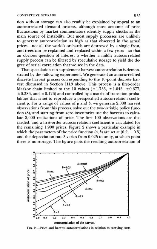
That speculation can supplement harvest autocorrelation is demon- strated by the following experiment. We generated an autocorrelated discrete harvest process corresponding to the 10-point discrete harvest discussed in Section IIIB above. This process is a first-order Markov chain limited to the 10 values (? 1.755, ? 1.045, ? 0.677, ? 0.386, and ? 0.126) and controlled by a matrix of transition probabilities that is set to reproduce a prespecified autocorrelation coefficient p. For a range of values of p and 8, we generate 2,000 harvest observations from this process, solve out the two-variable policy function (8), and starting from zero inventories use the harvests to calculate 2,000 realizations of price. The first 100 observations are dis- carded, and a first-order autocorrelation coefficient is calculated for the remaining 1,900 prices. Figure 2 shows a particular example in which the parameters of the price function (a, b) are set at (0.2, - 0.5) and the depreciation rate 8 varies from 0.025 to unity, at which point there is no storage. The figure plots the resulting autocorrelation of

? 0.0 0.1 0.2 0.3 0.4 0.5 0.6 0.7 0.8 0.9 1.0

Autocorrelation of the harvest FIG. 2.-Price and harvest autocorrelations in relation to carrying costs


prices against the autocorrelation of the harvests, together with the 45-degree line, which corresponds to a value of 8 of unity.

It is typically the case that the activity of the speculators increases the autocorrelation and that it does so by more the lower the cost of carrying inventories. When harvest autocorrelations are low, the speculation can have a large effect on the autocorrelation of prices; for the lowest values of 8 in the figure, the autocorrelation is increased from zero to more than 0.5. But as the autocorrelation of the harvest increases, the modulating effect of the speculators is less, so that although prices are still usually more autocorrelated than the harvests, the increment is smaller the higher the initial autocorrelation. These effects do not result from any decrease in storage at higher levels of autocorrelation; indeed, for all the cases shown in the figure, mean storage increases as one moves from left to right. However, the storage has less and less effect in increasing the autocorrelation of prices.

How much autocorrelation comes from the shocks and how much from speculation can be settled only by estimating the full model. The estimation follows the procedures in the i.i.d. case, at least in principle. For each price in the data, we calculate the expectation and variance of next period's price, feeding the results into the pseudo- likelihood function (17), which is then used as a guide to choose the parameters a, b, 8, and p. The calculation of the price function is more complex because it contains two arguments, the current harvest in addition to the amount on hand, but the approximation of the harvest process by a discrete Markov chain removes any serious difficulty. The hardest technical issue comes from the fact that, when the price function contains two arguments, we cannot solve back from the observed price to the amount on hand, but only to a set of combi- nations of amount on hand and harvest. In order to integrate over the various possibilities, we have to assume that prices have settled onto their invariant distribution, which has to be calculated and the results used to combine the price forecasts for the various combina- tions of harvest and amount on hand. Although straightforward enough in conception, the implementation has presented a number of difficulties that are described in the technical paper (Deaton and Laroque 1995).

The evaluation of the pseudo-likelihood function requires the first two moments of prices conditional on lagged price, and the calculation of these moments is illustrated in figure 3 (the conditional expectation) and figure 4 (the conditional variance). They are calculated for hypothetical parameters; note that the autocorrelation of the harvest process is taken to be 0.5, which is lower than the values that we shall obtain in the estimation. The three nonbold lines in figure 3 show


0.36 low harvest

8 0.32 -

o 0.28 - intermediate harvest 0

N 0.24 vI / high harvest

0.20/ with no information on harvest

i 0.16 -

0.12 - a=0.2, b=-0.2, 8=0.05, p=0.5

o 0.08 -

0.04 0.1 0.2 0.3 0.4 0.5 0.6 0.7 0.8 0.9

current price

FIG. 3.-One-period-ahead price expectations and harvest information

.8 0.020 - low harvest

a 0.016 intennediateharvest 0

0 0.012 high harvest\

08/ with no information on harvest

. 0.008

; 0.004 | a=0.2, b=-0.2, &0.05, p=0.5

> 0.000 0.1 0.2 0.3 0.4 0.5 0.6 0.7 0.8 0.9

current price

FIG. 4.-One-period-ahead price variances and harvest information

the conditional expectations from (11), that is, the one-period-ahead forecast of price conditional on both the current price and the current harvest. These autoregressions are piecewise linear, with slope (1 + r)/(l - 8) when pt ' p*(z) and zero when pt : p*(z). Because the harvests are assumed to be positively autocorrelated, the expected price next period is a decreasing function of the current harvest conditional on current price. For market participants, who observe the


harvest, these three lines would be the relevant predictors. The econometrician does not observe the harvest and must integrate out the harvests conditional on current price alone. As described above, this is done by weighting the conditional expectations by the probabilities of each harvest outcome conditional on the current price. The result is the bold line in figure 3, which is the conditional expectation that would be fed into the pseudo-likelihood function. This line coin- cides with the three light lines when prices are low enough so that storage takes place whatever the harvest, it smooths over the kinks at intermediate prices, and it continues to rise to the right because the weights shift to lower harvests at higher values of the current price.

Figure 4 illustrates the corresponding conditional variances, again with and without conditioning on the current harvest. These variance functions are monotone increasing, are constant above p*(z), but, unlike the conditional expectations, are nonlinear for prices less than p*(z). These graphs, together with the conditional expectation in figure 3, show that the first two conditional moments of prices under the storage model are quite different from those of a standard linear AR(1). (This property extends to higher moments, though our pseudo-maximum likelihood estimation methods do not use the information.) When the harvests are autocorrelated, as in figures 3 and 4, the conditional moment functions are differentiable. This is not the case in the i.i.d. model, because the econometrician's ignorance of the current harvest zt smooths over the nondifferentiability at p*(z). Note also that the nonlinearity of the price series under the model is affected by the value of the autocorrelation parameter p. The relevant case in our empirical results is the one in which p is large. Thus the bold line in figure 3 has a lower slope at low p and a higher slope at high p, so that its curvature is reduced and the conditional expectation is closer to the linear form of an AR(1). In consequence, an estimated storage model with a (highly) positively autocorrelated harvest is closer to the linear autoregression than the simpler storage model without autocorrelation.

High autocorrelation also exacerbates the technical and computational problems. For the current substantive purposes, these difficulties mean that the estimates here are presented only as those that generate the highest pseudo-likelihood values that we have been able to locate, albeit after a thorough and extensive search over a relatively small (four-) dimensional space. Furthermore, we have not been able to calculate useful estimates of standard errors. In spite of these problems, the Monte Carlo experiments reported in the companion paper show that the estimation procedure has reasonable success in recov- ering the parameters when the model is correct, and that it does so with some precision even for sample sizes like those used here. The


greatest difficulty is in the estimate of p, which was quite variable in our experiments; with the true p set at 0.5, the mean estimate over 100 replications was 0.40 with a standard deviation of 0.25.

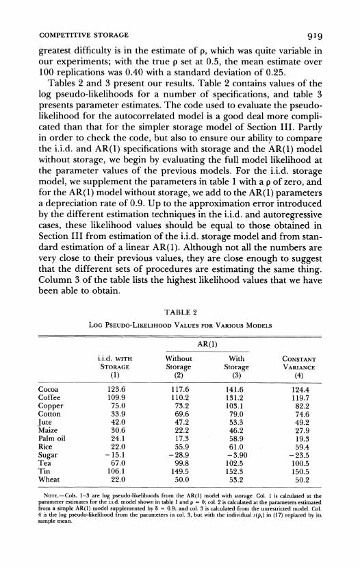
Tables 2 and 3 present our results. Table 2 contains values of the log pseudo-likelihoods for a number of specifications, and table 3 presents parameter estimates. The code used to evaluate the pseudo- likelihood for the autocorrelated model is a good deal more complicated than that for the simpler storage model of Section 111. Partly in order to check the code, but also to ensure our ability to compare the i.i.d. and AR(1) specifications with storage and the AR(1) model without storage, we begin by evaluating the full model likelihood at the parameter values of the previous models. For the i.i.d. storage model, we supplement the parameters in table 1 with a p of zero, and for the AR(1) model without storage, we add to the AR(1) parameters a depreciation rate of 0.9. Up to the approximation error introduced by the different estimation techniques in the i.i.d. and autoregressive cases, these likelihood values should be equal to those obtained in Section III from estimation of the i.i.d. storage model and from standard estimation of a linear AR(1). Although not all the numbers are very close to their previous values, they are close enough to suggest that the different sets of procedures are estimating the same thing. Column 3 of the table lists the highest likelihood values that we have been able to obtain.

TABLE 2 LOG PSEUDO-LIKELIHOOD VALUES FOR VARIOUS MODELS

AR(l)

i.i.d. WITH Without With CONSTANT STORAGE Storage Storage VARIANCE

(1) (2) (3) (4)

Cocoa 123.6 117.6 141.6 124.4 Coffee 109.9 110.2 131.2 119.7 Copper 75.0 73.2 103.1 82.2 Cotton 33.9 69.6 79.0 74.6 jute 42.0 47.2 53.3 49.2 Maize 30.6 22.2 46.2 27.9 Palm oil 24.1 17.3 58.9 19.3 Rice 22.0 55.9 61.0 59.4 Sugar - 15.1 - 28.9 -3.90 - 23.5 Tea 67.0 99.8 102.5 100.5 Tin 106.1 149.5 152.3 150.5 Wheat 22.0 50.0 53.2 50.2

NOTE.-COIS. 1-3 are log pseudo-likelihoods from the AR(l) model with storage. Col. 1 is calculated at the parameter estimates for the i.i.d. model shown in table 1 and p = 0; col. 2 is calculated at the parameters estimated from a simple AR(1) model supplemented by 8 = 0.9; and col. 3 is calculated from the unrestricted model. Col. 4 is the log pseudo-likelihood from the parameters in col. 3, but with the individual s(pt) in (17) replaced by its sample mean.


TABLE 3 PARAMETER ESTIMATES FOR AR(1) MODELS WITH AND WITHOUT STORAGE

a a-AR(l) b b-AR(l) 8 p

(1) (2) (3) (4) (5) (6)

Cocoa .226 .185 - .064 - .059 .083 .837 Coffee .245 .226 - .075 - .062 .036 .833 Copper .535 .455 -.246 -.096 -.046 .751 Cotton .862 .604 - .088 - .104 .010 .945 Jute .526 .591 - .154 - .137 .053 .741 Maize .731 .696 - .469 - .178 - .050 .720 Palm oil .412 .525 -.244 -.177 -.050 .864 Rice .609 .571 -.120 -.121 .027 .889 Sugar .683 .682 -.493 -.382 .112 .626 Tea .438 .483 - .053 - .076 .232 .918 Tin .223 .222 -.038 -.043 .046 .918 Wheat .680 .647 - .162 - .133 .051 .785

NOTE.-CoIs. 1, 3, 5, and 6 are the estimates of the parameters of the storage model with autocorrelated shocks. Cols. 2 and 4 are derived from the parameters of a first-order linear AR(1) model as described in the text; the autocorrelation parameter of the AR(1) model is (approximately) col. 5 of table 1 and is not repeated.

When interpreting the numbers in table 2, note that log pseudo- likelihood values do not behave like log likelihood values; in particular, twice the differences in log pseudo-likelihood values do not have asymptotic x2 distributions even when we are dealing with nested models. Nevertheless, the pseudo-likelihood values are useful as de- scriptive statistics of model fit; from (17), the pseudo-likelihood function penalizes variance, and it penalizes deviations from the one-step- ahead predictions and does so by more when a high variance is not predicted.

The parameter estimates for the storage model with autocorrelated shocks are listed in table 3. For comparison, we also include the corresponding parameter estimates from a linear first-order autoregression fitted to the prices. Given our normalization of the harvest, the parameter a of the storage model corresponds to the estimated mean of the AR(1), that is, the estimated constant in the autoregression divided by 1 - p, and the storage model parameter b to the variance of the innovation in the AR(1). By the same argument as in Section 111, the truth of the model would imply that the estimated a parameters should be less than mean prices or, equivalently, than the means of the estimated autoregressions. This condition fails for nine of the 12 commodities.

The pseudo-likelihood values for the AR(1) model with storage in column 3 of table 2 are larger than those for the restricted model, as they must be, by large margins for all commodities except tea, tin, and wheat. However, for three other goods, copper, maize, and palm


oil, the estimates of the depreciation parameter 8 have been forced to or close to its lower bound of - 0.05; see equation (20). While such estimates are substantively absurd, their effect is to drive to zero the cost of holding inventories, thus permitting large or infinite inventories that can be used to smooth prices in spite of the autocorrelation in the driving process. For these three goods, the estimates of the standard deviation in the absence of storage (b) are a good deal larger than the corresponding estimates from the AR(1) in column 4. For the other nine commodities, the best-fitting estimates show a marked similarity to those from the simple autoregression.

Given the similarity of the parameter estimates, why does the AR(1) model with storage yield higher pseudo-likelihood values than those from the autoregression without storage? Certainly, if we plot actual prices against one-period-ahead forecasts for the two models, there is little or no difference that is perceptible to the naked eye. A clue can be found by examining simulations of prices with and without storage. The differences between such price series come at low levels of prices, where the speculators enter the market and bid up prices by taking commodity into store for later resale. Because the optimal purchases are modest and resales are spread over the long subsequent boom, there is no perceptible effect in lowering prices when they are high. The effect of storage on prices is quite modest when the autocorrelation of the driving process is so large, as was also seen in the simulations in figure 2. However, the existence of storage has an effect not only on the mean of next period's price, but also on its variance. It is this effect that accounts for most of the improvement in the likelihood between column 3 and columns 1 and 2 of table 2. Column 4 of table 2 documents this by calculating the log pseudo- likelihood according to (17) but with the variances s(pt) replaced by their average value, a change that brings the likelihood most of the way back to that for the best of the other two models.

We find these results almost as disappointing as those for the storage model with i.i.d. harvests. We began our research from the relatively favorable results in Deaton and Laroque (1992) and with a reasonable expectation that the behavior of speculators could filter i.i.d. prices into the highly autocorrelated prices that we see in the data. Not only is that expectation disappointed, but so is the more limited ambition of attributing the autocorrelation partly to the driving processes of supply and demand and partly to the activities of the speculators. Instead, we are forced to attribute effectively all of it to the underlying processes. Although speculation is capable of increasing the autocorrelation that would otherwise exist in an un- moderated price series, it cannot raise it to the levels that we observe.


Appendix

Proof of Proposition 1

Letf(x, z) be the rational expectations equilibrium associated with the base economy, in which the harvests have zero mean and unit variance and the inverse demand function P(z) a + bz is linear. Denote by I(x, z) the amount of inventories carried forward when the amount on hand is x and the harvest is z. We know that, under some continuity and monotonicity requirements, [f(x, z), I(x, z)] is the unique solution of the following system of functional equations:

f(x,z) = max{l + ff[z' + (1 - 8)I(xz),z ]4 (z, ), P()}

(Al1) I(x,z) =x - P-'[(x,z)].

Consider now the alternative economy, with the same interest rate r and the same depreciation rate 8, where all magnitudes are denoted with tildes. This economy is characterized by a transition function for the harvests given by

and an inverse demand function

P(z) = (a _ ) b + b

z.

The rational expectations equilibrium of this economy is the solution of the system of functional equations (Al), with tildes over all the functions and variables. The proposition comes from the fact that there is a simple corre- spondence between the equilibria of the two economies. Let

x= X , z+ =

f(xz) =f(ux + pL,cz + A), I(x,z) = I + + A)

We start with the system of equations satisfied by the initial economy and show by substitution that (Al) also holds for the new economy. Consider the first equation. On the left-hand side, replacef(x, z) withf(x, Z). Similarly, on the right-hand side, substitute P5() for P(x) and D(Z, di') for (F(z, dz'), these quantities being equal by definition. Finally, it is straightforward to check that

f[z' + (1 - 8)I(x,z),z'] =f[urz' + IL(l - 8)uI(x,z),ucz' + A]

and is therefore equal toflz' + (1 - 8)I(x, 2), Z'].


It remains only to verify that a similar transformation applies to the second equation of (Al):

I(z, x) = x - P-[f(x, z)]

yields

I(g, )= U{x - P1[f(x, z)]} = x- _ - _ p- [f x, ZA

-- a

- -P-I[1(gZ)],

which completes the proof.

References

Chambers, Marcus J., and Bailey, Roy E. "A Theory of Commodity Price Fluctuations." Discussion Paper no. 432. Colchester: Univ. Essex, Dept. Econ., August 1994.

. "A Theory of Commodity Price Fluctuations." J.P.E. 104 (October 1996): 924-57.

Deaton, Angus, and Laroque, Guy. "On the Behaviour of Commodity Prices." Rev. Econ. Studies 59 (January 1992): 1-23.

. "Estimating a Nonlinear Rational Expectations Model with Unobserv- able State Variables." J. Apple. Econometrics 10 (1995): S9-S40.

Gilbert, Christopher L. "International Commodity Agreements: Design and Performance." World Development 15 (May 1987): 591-616.

Gourieroux, Christian; Monfort, Alain; and Trognon, Alain. "Pseudo Maxi- mum Likelihood Methods: Theory." Econometrica 52 (May 1984): 681-700.

Laroque, Guy, and Salanie, Bernard. "Estimating the Canonical Disequilib- rium Model: Asymptotic Theory and Finite Sample Properties." J. Econo- metrics 62 (June 1994): 165-210.

Newbery, David M. G., and Stiglitz, Joseph E. The Theory of Commodity Price Stabilization: A Study in the Economics of Risk. Oxford: Oxford Univ. Press, 1981.

Samuelson, Paul A. "Stochastic Speculative Price." Proc. Nat. Acad. Sci. 68 (February 1971): 335-37.

Williams, Jeffrey C., and Wright, Brian D. Storage and Commodity Markets. Cambridge: Cambridge Univ. Press, 1991.

Documents

Competitive Storage and Commodity Price Dynamicsdeaton/downloads/Competitive_Storage... · Competitive Storage and Commodity Price Dynamics Angus Deaton Princeton University Guy Laroque