Embed Size (px)
Citation preview
Abstract No.: 011-0368
Competition under Generalized Attraction Models: Applications to
Quality Competition under Yield Uncertainty
Awi Federgruen Graduate School of Business, Columbia University
New York, NY 10027 Email: [email protected]
Nan Yang
Johnson School of Management, Cornell University Ithaca, NY 14853
Email: [email protected]
POMS 20th Annual Conference Orlando, Florida U.S.A. May 1 to May 4, 2009
Submitted tomanuscript
Competition Under Generalized Attraction Models:Applications to Quality Competition Under Yield
Uncertainty
Awi FedergruenGraduate School of Business, Columbia University, New York, NY 10027, [email protected]
Nan YangJohnson School of Management, Cornell University, Ithaca, NY 14853, [email protected]
We characterize the equilibrium behavior in a broad class of competition models, in which the competing
firms’ market shares are given by an attraction model, and the aggregate sales in the industry depend on the
aggregate attraction value according to a general function. Each firm’s revenues and costs are proportional
with its expected sales volume, with a cost rate which depends on the firm’s chosen attraction value according
to an arbitrary increasing function.
While most existing competition papers with attraction models can be viewed as special cases of this
general model, we apply our general results to a new set of quality competition models. Here an industry
with N suppliers of a given product, compete for the business of one or more buyers. Each of the suppliers
encounters an uncertain yield factor, with a given, general yield distribution. The buyers face uncertain
demands over the course of a given sales season. The suppliers compete by selecting key characteristics of their
yield distributions, either their means, their standard deviations or both. These choices have implications
for their per unit cost rates.
1. Introduction and Summary
Starting with a seminal paper by Friedman (1958), there is a well established tradition in the economics,
marketing and operations literature to model competition in oligopolies by assuming that the firms’
sales volumes are specified by a so-called attraction model, see, e.g. Lilien et al. (1992), Cooper (1993),
Karnani (1985), Anderson et al. (1992), Besanko et al. (1998), So (2000) and Gallego et al. (2006). In
an attraction model, each firm’s strategic choices determine a single “attraction value”, such that his
market share is given by the ratio of this attraction value and the sum of the industry’s values. Bell et al.
(1975) have shown that this is, in fact, the only representation of market shares to satisfy four simple
axioms. With market shares determined by the above ratio rule, the firm’s expected sales volumes are
1
Federgruen and Yang: Competition Under Generalized Attraction Models
2 Article submitted to ; manuscript no.
completely determined by a specification of the aggregate sales in the industry, only. The latter is, most
commonly, assumed to be a constant, i.e., independent of the strategic choices, or to increase towards
this constant potential market size according to a very specific function of the aggregate attraction
value, see (2) below.1 However, starting with Kotler (1965), several papers have modeled aggregate
sales as a general function of the aggregate attraction value in the industry, see also Bell et al. (1975),
Karnani (1985) and Basuroy and Nguyen (1998).
While in many settings, aggregate sales should be represented as an increasing function of the aggre-
gate attraction value, there are models in which aggregate sales decrease as this value improves. This
includes the model which motivated our paper and to which we devote its second part. Here, alterna-
tive suppliers of a common good compete with each other in terms of certain characteristics of their
uncertain yield processes, for example the reliability of each manufacturing batch’s yield factor. In this
model, which considers either a single buyer or a finite set of buyers, it is in fact possible to derive the
suppliers’ sales volumes explicitly by identifying the optimal procurement policy of each of the buyers.
(Most competition models assume a specific functional form of the demand functions as exogenously
given.) The resulting expected sales volumes imply market shares given by an attraction model with
a reliability measure serving as the attraction value; however, as the suppliers improve their reliabil-
ity, aggregate purchases by the buyers decline, the reduced supply risks reducing the need for safety
stocks. Thus, when an individual supplier increases his yield reliability, this results in an increase of his
market share, although not necessarily of his expected sales volume. Since the per unit manufacturing
cost increases with the selected yield reliability, the yield improvement also results in a reduced profit
margin, thus giving rise to intricate sets of tradeoffs.
In this paper, we analyze a general competition model, with market shares determined by an attrac-
tion model, and aggregate sales specified as a general function of the aggregate attraction value. Firms
compete with each other by selecting their attraction value, which impacts the firm’s market share,
aggregate sales as well as the per unit cost incurred. Competition models in our literature tend to focus
on sufficient conditions with respect to the input parameters and functions, to guarantee the existence
1 If X denotes the aggregate of the attraction values in the industry, the total sales in the industry is given by a functionof the form MX/(X + C), with M,C > 0 given constants.
Federgruen and Yang: Competition Under Generalized Attraction Models
Article submitted to ; manuscript no. 3
of a (pure) Nash equilibrium, possibly in conjunction with its uniqueness. The perspective in this paper
is to provide a full characterization of the equilibrium behavior under arbitrary model parameters and
cost functions. Often, there are multiple equilibria, in which case we fully characterize their number and
relative position vis-a-vis each other. We also show how, in the fully general model, the entry or exit of
a supplier impacts on the equilibria. We summarize our main results by describing their application to
the above quality competition model. (See also §5 for a summary, in the context of the general model.)
To motivate the latter, note that in most industries, component suppliers or original equipment
manufacturers (OEMs) increasingly compete in terms of product attributes other than direct cost. Many
goods have become commoditized, and gross profit margins have shrunk, making it increasingly difficult
to compete on the basis of price differentials (alone). The supplier’s quality and his yield effectiveness
and reliability, as measured by the percentage of effectively produced units, rank among the most critical
of the various dimensions along which competing firms differentiate themselves. The same applies to
suppliers of consumer goods to large department stores, retail organizations or government agencies
(in the latter case, e.g., vaccines or medical devices). The yield characteristics include the possibility
of complete disruptions due to natural causes, such as fires or hurricanes, man made breakdowns (e.g.
sabotage or terrorist attacks), as well as bankruptcies2. Many companies have adopted a multi-sourcing
strategy, splitting orders among competing suppliers so as to mitigate various supplier risks.
Our quality competition model considers an industry with N potential suppliers competing for the
business of B buyers, in a single sales season. To facilitate the exposition, we initially consider a single
purchasing firm or agency. However, almost all of our results carry over to the general oligopsony case
with an arbitrary number of buyers, see Appendix EC.4. The purchasing firm faces an uncertain demand
volume, while each of the suppliers experiences a given random yield factor. In the face of the combined
2 Even before the 2008 financial crisis, Babich et al. (2007) describe the severity of this type of risk: “Credit rating firmsreport that in 2002 over 240 firms defaulted on 160 billion dollars of debt, the largest amount ever over any one year period.. . . The combined volume of defaults in 2001 and 2002 exceeded the total volume of defaults in the US over the previoustwenty years. What is especially striking about the current trends is the surge in the defaults of large, well-establishedcompanies. Even in the relative stable years 2000-2005, almost 50 firms with assets or liabilities exceeding one billiondollars have filed for bankruptcy.”In the automobile industry, for example, many suppliers routinely incur losses, with Delphi, the largest supplier of auto-motive parts in the United States, residing in Chapter 11, until recently. Choi and Hartley (1996) document that in thisindustry, purchasing managers consider the financial solvability of the suppliers a major selection criterion, along withcriteria like consistency and reliability.
Federgruen and Yang: Competition Under Generalized Attraction Models
4 Article submitted to ; manuscript no.
demand and supply risks, the buyer determines a total order size and its allocation among the potential
suppliers, minimizing purchasing costs while ensuring that a shortfall is avoided with a given minimum
probability. Imperfect yields represent a problem for the buyer, only to the extent the yield factor
is uncertain: a consistent, imperfect yield factor p, can be handled, trivially, by inflating any desired
supply quantity by the factor p−1. As will become apparent in the analysis, the key characteristic of the
yield distribution is its coefficient of variation, or the supplier’s reliability, defined as the reciprocal of
the squared coefficient of variation. We show that this reliability measure is bounded from below by a
positive constant. This endogenously determined minimum value may, sometimes, need to be increased
due to standards imposed externally by the buyers or a regulatory agency, see §4 for examples.
A supplier can improve his reliability by (i) increasing the yield predictability, via a reduction of
the standard deviation of the yield factor, or (ii) increasing the yield target, i.e. the mean of the yield
distribution, or (iii) improving both the yield target and its standard deviation. Depending on the
source(s) behind his random yields, a supplier may improve the coefficient of variation of his yield
distribution, by investing more time and effort into the design phase, or by adopting appropriate
technologies, materials, manufacturing and logistical processes or a more secure financial structure, as
well as improving his facilities’ security. Depending on which of the settings (i), (ii) or (iii) prevails, we
distinguish between three types of competition, which we refer to, respectively, as (I) Yield Predictability
Competition, (II) Yield Target Competition, and (III) Simultaneous Yield Target and Predictability
Competition. To focus on the impact yield targets and reliabilities have on the suppliers’ competitive
position, we initially assume that they charge a uniform price. As many industries become increasingly
commoditized, this assumption often applies, per se. See, however, §4.4 for a discussion of the general
case with supplier-dependent prices. (Even though the suppliers’ goods are perfect substitutes, more
reliable suppliers may be able to charge more than others.)
The competition models are Stackelberg games, in which the suppliers compete by making yield
choices and the purchasing firm follows by determining how much she wants to order from each. Starting
with the Yield Predictability Competition model, we show that this model always has an equilibrium,
as long as the aggregate of the suppliers’ minimum reliability standards is in excess of a threshold
Federgruen and Yang: Competition Under Generalized Attraction Models
Article submitted to ; manuscript no. 5
value, given by a simple function of the permitted shortfall probability. (If this condition is violated,
the buyer may not be able to satisfy her service constraint, under certain yield choices of the suppliers;
see, below, for a characterization of the equilibrium behavior in this case.) Under multiple equilibria,
there exists one which is componentwise smallest and one which is componentwise largest. Among
all equilibria, the former is the most preferred, and the latter the least preferred, by all suppliers,
while the opposite applies to the buyer. Also, under convex manufacturing cost rates, for example,
all equilibria are completely ordered, i.e., if one supplier adopts a higher reliability measure under
one equilibrium as opposed to an alternative equilibrium, the same applies to all of his competitors.
In our numerical studies, we have observed that multiple equilibria arise frequently, and the largest
and smallest equilibria are often far apart. Assuming suppliers dynamically adjust their yield choices
(e.g., as best responses to the competitors’ choices), the industry’s equilibrium depends heavily on its
initial choices: for example, if all suppliers start out with low (high) yield reliabilities, we show that
the industry adopts the smallest (largest) equilibrium. This suggests that there is great permanent
value to adopt short term incentives (e.g., the imposition of the above minimum reliability standards)
for suppliers to invest in yield improvements. Because of the competitive dynamics, such short term
incentives sustain themselves in the long run.
Any equilibrium is characterized by a set of suppliers which operate at their minimum standard
level and a complementary set which choose to go beyond their minimum. We show that when each
firm’s per unit production cost grows convexly with its chosen yield reliability, the set of “minimum
performance” suppliers is consecutive in a specific supplier index. This index depends on the supplier’s
minimum reliability standard and his marginal cost rate and profit margin when operating at this
reliability level. Finally, under an additional condition, broadly satisfied, we derive a bound for the
number of distinct equilibria. We show that improving the minimum standards may eliminate a low
performance equilibrium and drive the suppliers to one in which they very significantly outperform
these standards. Thereafter, the high performance equilibrium is often self-sustaining, even when the
minimum standards are no longer enforced.
We show that, under both the smallest and the largest equilibrium, all suppliers react to a sales price
decrease by investing in a lower yield reliability. (All of the comparative statistics results, described
Federgruen and Yang: Competition Under Generalized Attraction Models
6 Article submitted to ; manuscript no.
below, refer, likewise, to the smallest and largest equilibrium.) In settings where the buyer has the
bargaining power to reduce the sales price, exercising this power has the, perhaps unintended, conse-
quence of incentivizing all suppliers to reduce their reliability investments. This phenomenon has been
documented, for example, in the vaccine supply industry, see §4.
When a single supplier is able to increase his yield target, i.e., the mean of his yield distribution, all
suppliers increase their yield reliability. We also show that every new entrant to the market causes all
incumbents to improve their yield reliability; conversely, every departure from the industry induces all
remaining firms to reduce it. When the mean demand volume goes up, the suppliers react by reducing
their yield reliability, but when the standard deviation of the demand volume goes up, they respond
by increasing their yield reliability. More comprehensively, we show that suppliers find it in their
competitive interest to respond to increased volatility of the buyer’s demand volume, i.e., an increased
coefficient of variation of the demand distribution, by increasing their yield reliability; at the same time,
they exploit increased risk averseness of the buyer, i.e., a lower tolerance for the shortfall probability,
by reducing their equilibrium yield reliability so as to force the buyer to increase purchase orders.
In symmetric models, there exists a critical number of suppliers N 0(x) – which depends on the
minimal standard x – such that the equilibrium is unique (and larger than the minimum standard) if
the number of suppliers N is in excess of N 0(x). If N is smaller than this critical number of firms, the
minimum standard x represents one equilibrium, possibly in conjunction with one or two symmetric
equilibria in which all suppliers adopt a common higher reliability value.
We obtain similar characterizations of the equilibrium behavior, for the other two competition mod-
els. The remainder of this paper is organized as follows: in §2, we provide an overview of the related
literature. In §3, we characterize the equilibrium behavior in the above defined general class of competi-
tion models. §4 applies the results of §3 to the aforementioned quality competition models. §5 concludes
the paper with a summary of important conclusions. All proofs are relegated to EC.1.
2. Literature Review
In §1, we have surveyed the literature on competition under attraction models. In this section, we give
a brief review of the literature directly relevant to the quality competition model.
Federgruen and Yang: Competition Under Generalized Attraction Models
Article submitted to ; manuscript no. 7
The economics literature treats quality as a differentiating attribute of the product rather than its
procurement process; see Appendix EC.2 for a brief review.
Very few papers analyze the impacts of uncertain yields in decentralized supply chains. The recent
paper by Zhu et al. (2007) comments in its opening paragraph, “Although researchers in operations
management have long realized the importance of operations beyond the walls of a firm and explored
various management issues for better coordination along supply chains, research on quality improvement
has been largely limited to operations inside the walls of a firm.” Likewise, in their survey paper, Tsay
et al. (1999) note that only a few models consider the choice of the quality level, and, if so, primarily
“from the vantage point of a single organization contemplating how to design its internal practices in
light of its own costs of quality.”Zhu et al. (2007) analyze a model with a single supplier and a single
buyer facing a deterministic demand process, in which the buyer and the supplier sequentially decide
to invest in an improvement of the yield characteristics of the supplier’s production process. Babich
et al. (2007) consider an industry with two suppliers and one buyer. Particularly motivated by the
risk of suppliers’ defaulting and therefore not being able to deliver on their orders, the authors assume
that each supplier’s random yield factor is a Bernoulli random variable, which is equal to zero, with a
probability given by the firm’s likelihood of default. The two firms compete by selecting a unit price.
Corbett and Deo (2006) assume that an arbitrary number of suppliers, offering a homogenous good,
engage in Cournot competition, where the (common) per unit price is a linear function of the total
actual supply offered to the market. (A firm’s actual supply is its intended production volume multiplied
with a random yield factor, which is independently generated from a common distribution.) The firms
compete by selecting their intended production volumes. Corbett and Deo (2006) use their model to
explain the number of flu vaccine suppliers in the United States. Chick et al. (2006) consider a supply
chain with a single buyer and a single supplier, whose random yield factor follows a general distribution.
The buyer derives a benefit from its order, the magnitude of which grows as a concave function of the
order size.3 The authors characterize how the buyer and the supplier sequentially determine their order
3 The authors are, again, particularly motivated by the flu vaccine supply problem, where this benefit function relates tothe national cost savings due to a larger fraction of the population being vaccinated.
Federgruen and Yang: Competition Under Generalized Attraction Models
8 Article submitted to ; manuscript no.
size and intended production volume. To our knowledge, ours is the first model to analyze a supply
chain in which suppliers compete by targeting key characteristics of their uncertain yield processes.
3. Competition Under a General Attraction Model
Consider an industry with N firms, each selling a specific good or service, at a given unit price. As in
standard attraction models, each firm i’s market share is proportional to its attraction value xi, which
can be selected within a given range [xi, xi] (i = 1, . . . ,N). The attraction values sometimes denote a
single strategic choice, for example, the firm’s advertising budget in Friedman (1958), or the firm’s
manufacturing yield reliability in the quality competition model of §4. In other settings, it is a function
of, several strategic choices: to give but a few examples, in the combined price and quality multinomial
logit competition model in Anderson et al. (1992), the attraction value is an exponential function of
a linear combination of the firm’s price and quality level. In Bernstein and Federgruen (2004), the
attraction value is a general function of the firm’s price and service level, characterized by its fill-rate.
Kotler (1965) specifies the attraction value as a function of the firm’s price, advertising and distribution
budget, while Carpenter et al. (1988) model it as a function of a variety of marketing instruments.
As to the aggregate expected sales in the industry, we assume that it is determined by the aggregate
attraction value. The cost incurred by a firm is proportional to its sales volume, with a cost rate which
is nondecreasing in the firm’s attraction value. This assumption is made in many competition papers
with attraction models, for example, the quality competition model in Anderson et al. (1992, §7.5.2),
or the price-service level competition model of Bernstein and Federgruen (2004), in which all costs are
shown to be proportional with the expected sales volume, at a rate which is increasing and convex in
the chosen fill-rate or attraction value. Gallego et al. (2006) [Besanko et al. (1998), So (2000)] assume
that the operational cost of each supplier is given by a convex [linear] function of his demand volume,
the shape of which is independent of the strategic choices.4 Thus, let
si = the expected sales volume of firm i, i = 1, . . . ,N
4 A natural generalization of our model would allow for fixed costs that are dependent on the chosen attraction valuesas well. However, this generalization significantly complicates the equilibrium analysis. (Among competition papers withattraction demand models, Karnani (1985) and Anderson et al. (1992, §7.5.3) consider fixed costs which depend on thestrategic choices, however, assuming that the variable cost rates are completely independent of these.)
Federgruen and Yang: Competition Under Generalized Attraction Models
Article submitted to ; manuscript no. 9
wi = the per unit sales price of firm i, i = 1, . . . ,N
ci(xi) = the per unit cost rate of firm i, a nondecreasing, twice differentiable function of the attraction
value xi, i = 1, . . . ,N
The assumptions of the generalized attraction model imply that
si = T
(N∑
j=1
xj
)· xi∑N
j=1 xj
, i = 1, . . . ,N, (1)
where T (·) describes how the total market size varies with the chosen attraction values x. Many models
specify T (·) as a constant M . Other papers use the specification
T (R) =MR
(R +C)(2)
This total sales function arises when assuming a given population of M individuals, each of whom
either purchase one unit from one of the firms or nothing at all, C represents the attraction value of the
no-purchase option, and the likelihood of an individual choosing a specific option is proportional to its
attraction value. Several marketing papers, including Kotler (1965), Karnani (1985) and Basuroy and
Nguyen (1998), assume T (R) = MRβ for some 0 6 β < 1 to represent a market which increases with the
aggregate attraction value, however at a decreasing marginal rate. While all of the above specifications
use an increasing T (·) function, the endogenously derived total sales function in the quality competition
model of §4 is, in fact, decreasing for reasons explained in the Introduction; see (12) for its closed form
expression. Below, we take T (·) as a general, twice differentiable function.
The lower bounds {xi} are sometimes endogenous to the model. In other settings, these bounds are
exogenously imposed by company policies or government regulations, see e. g. §4. As to the upper
bounds {xi}, if limxi→∞ ci(xi) > wi, only xi 6 inf{xi : ci(xi) > wi} represent relevant choices for firm i, to
ensure a nonnegative profit value. In the analysis below, we therefore assume xidef= inf{xi : ci(xi) > wi};
all of our results are easily extended when these upper bounds need to be specified at lower levels.
Firm i’s expected profit function is given by:
πi(x) =(wi − ci(xi)
)si =
(wi − ci(xi)
)(xi∑N
j=1 xj
)T
(N∑
j=1
xj
).
Federgruen and Yang: Competition Under Generalized Attraction Models
10 Article submitted to ; manuscript no.
With x−i =∑
j 6=i xj, it is easier to employ
πi(x)def= logπi(x) = log
(wi − ci(xi)
)+ logxi + log
[T (xi +x−i)
xi +x−i
], with (3)
∂πi
∂xi
= Gi(xi)−H(xi +x−i), where (4)
Gi(xi) =−c′i(xi)
wi − ci(xi)+
1
xi
, and H(R) =
{log
[R
T (R)
]}′
(5)
Thus, the marginal profit increase of a firm due to a marginal increase in his attraction value, depends on
the competitors’ strategic choices, only via their sum, x−i. The dependence is captured by the function
H(∑N
j=1 xj
)= ∂ log
(∑N
j=1 xj
/T(∑N
j=1 xj
))/∂xi, the marginal increase in the logarithm of the
aggregate required attraction value per unit sold, due to an increase in firm i’s attraction value (or that
of any firm, for that matter). When the total sales function T (·) is monotone – as is the case in all above
examples – H(R) represents the elasticity of the industry’s aggregate attraction value with respect to
its sales. The function A(R)def= R/T (R) denotes the required attraction intensity, i. e. the aggregate
required attraction value per unit sold. The following property of this function plays a fundamental
role in the equilibrium behavior of the competition model:
(A): The attraction intensity A(R) = R/T (R) is log-concave in R.
Theorem 1 (Existence of Equilibria). Assume (A).
(a) The competition game is (log-)supermodular and has at least one equilibrium. The set of equilibria
is a lattice; in particular, there exists a componentwise smallest equilibrium x∗ and a componentwise
largest equilibrium x∗.
(b) If the attraction intensity A(R) is increasing, we have that among all equilibria, x∗ [x∗] maxi-
mizes [minimizes] the expected profit for all firms.
We note that the attraction intensity function A(R) = R/T (R) is both log-concave and increasing
in all of the above examples. This is easily verified for the case where the aggregate sales function
T (R) is constant, or of the form (2) or a power function T (R) = MRβ with 0 6 β < 1. We refer to
Lemma 1, below, for a verification of these properties in the quality competition model of §4. Since the
competition model is a supermodular game, both the smallest and largest equilibrium can be computed
Federgruen and Yang: Competition Under Generalized Attraction Models
Article submitted to ; manuscript no. 11
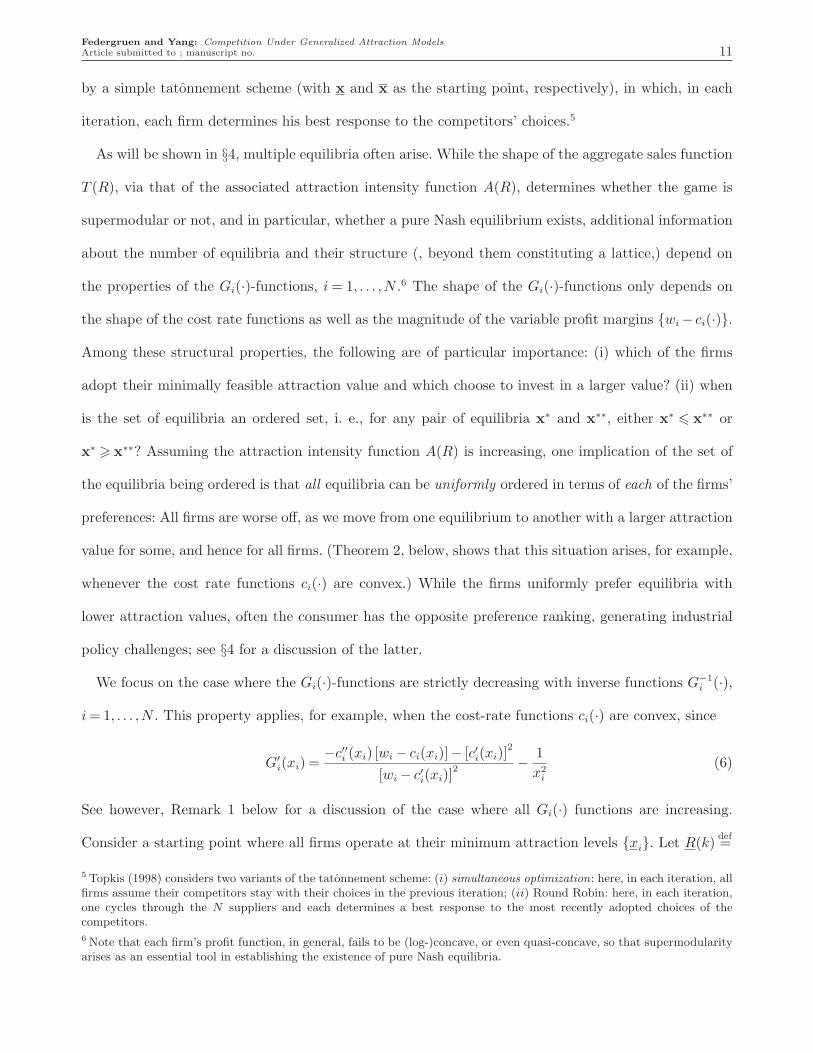
by a simple tatonnement scheme (with x and x as the starting point, respectively), in which, in each
iteration, each firm determines his best response to the competitors’ choices.5
As will be shown in §4, multiple equilibria often arise. While the shape of the aggregate sales function
T (R), via that of the associated attraction intensity function A(R), determines whether the game is
supermodular or not, and in particular, whether a pure Nash equilibrium exists, additional information
about the number of equilibria and their structure (, beyond them constituting a lattice,) depend on
the properties of the Gi(·)-functions, i = 1, . . . ,N .6 The shape of the Gi(·)-functions only depends on
the shape of the cost rate functions as well as the magnitude of the variable profit margins {wi − ci(·)}.
Among these structural properties, the following are of particular importance: (i) which of the firms
adopt their minimally feasible attraction value and which choose to invest in a larger value? (ii) when
is the set of equilibria an ordered set, i. e., for any pair of equilibria x∗ and x∗∗, either x∗ 6 x∗∗ or
x∗ > x∗∗? Assuming the attraction intensity function A(R) is increasing, one implication of the set of
the equilibria being ordered is that all equilibria can be uniformly ordered in terms of each of the firms’
preferences: All firms are worse off, as we move from one equilibrium to another with a larger attraction
value for some, and hence for all firms. (Theorem 2, below, shows that this situation arises, for example,
whenever the cost rate functions ci(·) are convex.) While the firms uniformly prefer equilibria with
lower attraction values, often the consumer has the opposite preference ranking, generating industrial
policy challenges; see §4 for a discussion of the latter.
We focus on the case where the Gi(·)-functions are strictly decreasing with inverse functions G−1i (·),
i = 1, . . . ,N . This property applies, for example, when the cost-rate functions ci(·) are convex, since
G′i(xi) =
−c′′i (xi) [wi − ci(xi)]− [c′i(xi)]2
[wi − c′i(xi)]2 − 1
x2i
(6)
See however, Remark 1 below for a discussion of the case where all Gi(·) functions are increasing.
Consider a starting point where all firms operate at their minimum attraction levels {xi}. Let R(k)def=
5 Topkis (1998) considers two variants of the tatonnement scheme: (i) simultaneous optimization: here, in each iteration, allfirms assume their competitors stay with their choices in the previous iteration; (ii) Round Robin: here, in each iteration,one cycles through the N suppliers and each determines a best response to the most recently adopted choices of thecompetitors.
6 Note that each firm’s profit function, in general, fails to be (log-)concave, or even quasi-concave, so that supermodularityarises as an essential tool in establishing the existence of pure Nash equilibria.
Federgruen and Yang: Competition Under Generalized Attraction Models
12 Article submitted to ; manuscript no.
∑k
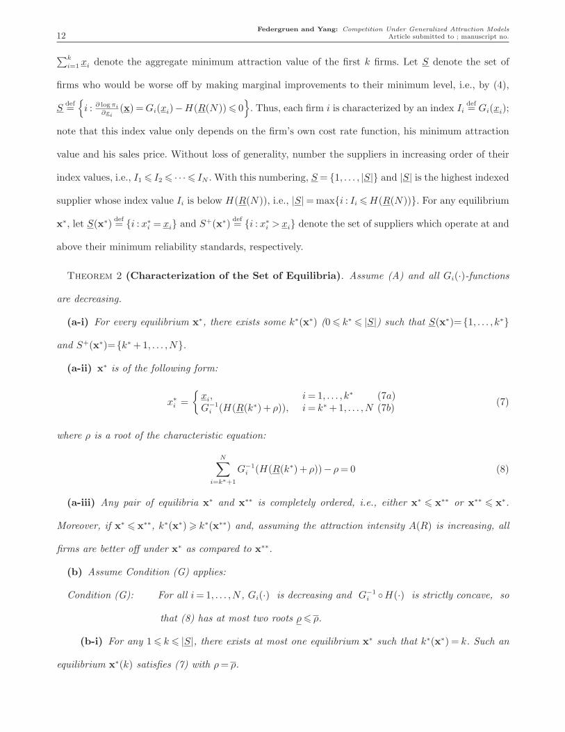
i=1 xi denote the aggregate minimum attraction value of the first k firms. Let S denote the set of
firms who would be worse off by making marginal improvements to their minimum level, i.e., by (4),
Sdef={i : ∂ logπi
∂xi(x) = Gi(xi)−H(R(N)) 6 0
}. Thus, each firm i is characterized by an index Ii
def= Gi(xi);
note that this index value only depends on the firm’s own cost rate function, his minimum attraction
value and his sales price. Without loss of generality, number the suppliers in increasing order of their
index values, i.e., I1 6 I2 6 · · ·6 IN . With this numbering, S = {1, . . . , |S|} and |S| is the highest indexed
supplier whose index value Ii is below H(R(N)), i.e., |S|= max{i : Ii 6 H(R(N))}. For any equilibrium
x∗, let S(x∗)def= {i : x∗
i = xi} and S+(x∗)def= {i : x∗
i > xi} denote the set of suppliers which operate at and
above their minimum reliability standards, respectively.
Theorem 2 (Characterization of the Set of Equilibria). Assume (A) and all Gi(·)-functions
are decreasing.
(a-i) For every equilibrium x∗, there exists some k∗(x∗) (0 6 k∗ 6 |S|) such that S(x∗)={1, . . . , k∗}
and S+(x∗)={k∗ +1, . . . ,N}.
(a-ii) x∗ is of the following form:
x∗i =
{xi, i = 1, . . . , k∗ (7a)G−1
i (H(R(k∗)+ ρ)), i = k∗ +1, . . . ,N (7b)(7)
where ρ is a root of the characteristic equation:
N∑
i=k∗+1
G−1i (H(R(k∗)+ ρ))− ρ = 0 (8)
(a-iii) Any pair of equilibria x∗ and x∗∗ is completely ordered, i.e., either x∗ 6 x∗∗ or x∗∗ 6 x∗.
Moreover, if x∗ 6 x∗∗, k∗(x∗) > k∗(x∗∗) and, assuming the attraction intensity A(R) is increasing, all
firms are better off under x∗ as compared to x∗∗.
(b) Assume Condition (G) applies:
Condition (G): For all i = 1, . . . ,N , Gi(·) is decreasing and G−1i ◦H(·) is strictly concave, so
that (8) has at most two roots ρ 6 ρ.
(b-i) For any 1 6 k 6 |S|, there exists at most one equilibrium x∗ such that k∗(x∗) = k. Such an
equilibrium x∗(k) satisfies (7) with ρ = ρ.
Federgruen and Yang: Competition Under Generalized Attraction Models
Article submitted to ; manuscript no. 13
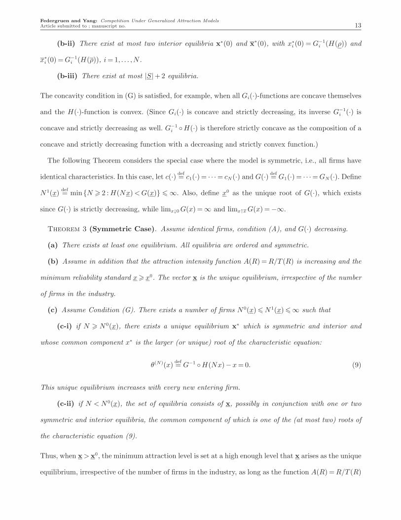
(b-ii) There exist at most two interior equilibria x∗(0) and x∗(0), with x∗i (0) = G−1
i (H(ρ)) and
x∗i (0) = G−1
i (H(ρ)), i = 1, . . . ,N .
(b-iii) There exist at most |S|+2 equilibria.
The concavity condition in (G) is satisfied, for example, when all Gi(·)-functions are concave themselves
and the H(·)-function is convex. (Since Gi(·) is concave and strictly decreasing, its inverse G−1i (·) is
concave and strictly decreasing as well. G−1i ◦H(·) is therefore strictly concave as the composition of a
concave and strictly decreasing function with a decreasing and strictly convex function.)
The following Theorem considers the special case where the model is symmetric, i.e., all firms have
identical characteristics. In this case, let c(·) def= c1(·) = · · ·= cN(·) and G(·) def
= G1(·) = · · ·= GN(·). Define
N 1(x)def= min{N > 2 : H(Nx) < G(x)} 6 ∞. Also, define x0 as the unique root of G(·), which exists
since G(·) is strictly decreasing, while limx↓0 G(x) =∞ and limx↑x G(x) =−∞.
Theorem 3 (Symmetric Case). Assume identical firms, condition (A), and G(·) decreasing.
(a) There exists at least one equilibrium. All equilibria are ordered and symmetric.
(b) Assume in addition that the attraction intensity function A(R) = R/T (R) is increasing and the
minimum reliability standard x > x0. The vector x is the unique equilibrium, irrespective of the number
of firms in the industry.
(c) Assume Condition (G). There exists a number of firms N 0(x) 6 N 1(x) 6∞ such that
(c-i) if N > N 0(x), there exists a unique equilibrium x∗ which is symmetric and interior and
whose common component x∗ is the larger (or unique) root of the characteristic equation:
θ(N)(x)def= G−1 ◦H(Nx)−x = 0. (9)
This unique equilibrium increases with every new entering firm.
(c-ii) if N < N 0(x), the set of equilibria consists of x, possibly in conjunction with one or two
symmetric and interior equilibria, the common component of which is one of the (at most two) roots of
the characteristic equation (9).
Thus, when x > x0, the minimum attraction level is set at a high enough level that x arises as the unique
equilibrium, irrespective of the number of firms in the industry, as long as the function A(R) = R/T (R)
Federgruen and Yang: Competition Under Generalized Attraction Models
14 Article submitted to ; manuscript no.
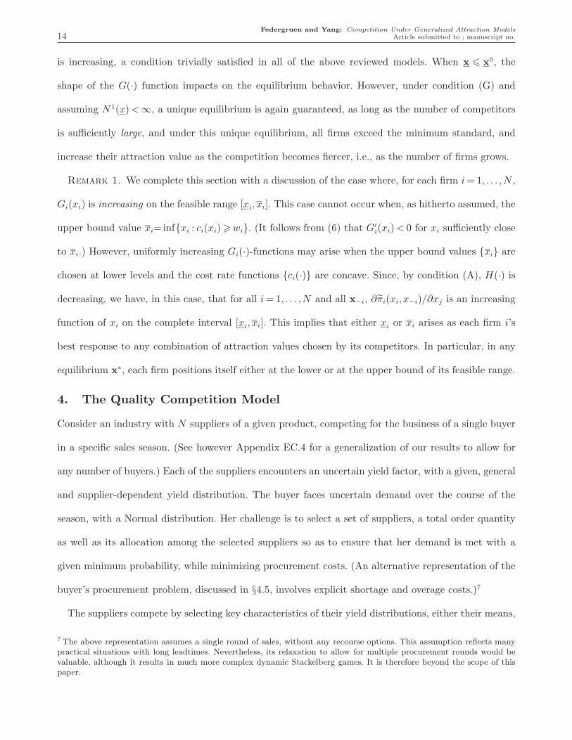
is increasing, a condition trivially satisfied in all of the above reviewed models. When x 6 x0, the
shape of the G(·) function impacts on the equilibrium behavior. However, under condition (G) and
assuming N 1(x) <∞, a unique equilibrium is again guaranteed, as long as the number of competitors
is sufficiently large, and under this unique equilibrium, all firms exceed the minimum standard, and
increase their attraction value as the competition becomes fiercer, i.e., as the number of firms grows.
Remark 1. We complete this section with a discussion of the case where, for each firm i = 1, . . . ,N ,
Gi(xi) is increasing on the feasible range [xi, xi]. This case cannot occur when, as hitherto assumed, the
upper bound value xi=inf{xi : ci(xi) > wi}. (It follows from (6) that G′i(xi) < 0 for xi sufficiently close
to xi.) However, uniformly increasing Gi(·)-functions may arise when the upper bound values {xi} are
chosen at lower levels and the cost rate functions {ci(·)} are concave. Since, by condition (A), H(·) is
decreasing, we have, in this case, that for all i = 1, . . . ,N and all x−i, ∂πi(xi, x−i)/∂xj is an increasing
function of xi on the complete interval [xi, xi]. This implies that either xi or xi arises as each firm i’s
best response to any combination of attraction values chosen by its competitors. In particular, in any
equilibrium x∗, each firm positions itself either at the lower or at the upper bound of its feasible range.
4. The Quality Competition Model
Consider an industry with N suppliers of a given product, competing for the business of a single buyer
in a specific sales season. (See however Appendix EC.4 for a generalization of our results to allow for
any number of buyers.) Each of the suppliers encounters an uncertain yield factor, with a given, general
and supplier-dependent yield distribution. The buyer faces uncertain demand over the course of the
season, with a Normal distribution. Her challenge is to select a set of suppliers, a total order quantity
as well as its allocation among the selected suppliers so as to ensure that her demand is met with a
given minimum probability, while minimizing procurement costs. (An alternative representation of the
buyer’s procurement problem, discussed in §4.5, involves explicit shortage and overage costs.)7
The suppliers compete by selecting key characteristics of their yield distributions, either their means,
7 The above representation assumes a single round of sales, without any recourse options. This assumption reflects manypractical situations with long leadtimes. Nevertheless, its relaxation to allow for multiple procurement rounds would bevaluable, although it results in much more complex dynamic Stackelberg games. It is therefore beyond the scope of thispaper.
Federgruen and Yang: Competition Under Generalized Attraction Models
Article submitted to ; manuscript no. 15
their standard deviations or both.8 These choices have implications for their per unit cost rates. We
initially assume that the suppliers’ prices are identical. This assumption often applies per se, as many
industries have become commoditized.9 (In §4.4, we discuss the general case, where the suppliers dif-
ferentiate themselves on the basis of their prices, as well.) The suppliers operate in a make-to-order
or purchase-to-order environment, which permits them to defer commitment to all material and other
variable costs until the buyer’s orders are received.
We also assume that the buyer only pays for delivered units which are useable, i.e., satisfy the
quality standards. This assumption is adopted by the majority of the literature on random yield supply
systems.10 The practitioner oriented outsourcing literature, e. g., Brown and Wilson (2005), refers to
this as fixed pricing schemes. (In §4.4, we analyze other settings, where the buyer is required to pay for
all units ordered and entered into the production process, or where the buyer incurs two cost rates, one
that applies to all units ordered and the other which is charged only for the useable ones.) Thus, let:
Xi = the random yield factor at supplier i’s facility, with mean pi, variance ς2i , coefficient of
variation γi = ςi/pi, and reliability measure xidef= γ−2
i = p2i /ς2
i , i = 1, . . . ,N ;
D = the uncertain demand during the season, which is Normally distributed with mean µ,
variance σ2, and coefficient of variation γD = σ/µ;
ci(pi, ςi) = the expected cost for supplier i to procure an effective unit, a twice differentiable function, with
limςi↓0
ci(pi, ςi) = limpi↑1
ci(pi, ςi) = +∞;
w = the price charged to the buyer for every effectively delivered unit;
α = maximum permitted probability of a shortfall;
8 In the Electronic Design Automation (EDA) industry, manufacturers focus their competitive strategies on “Design ForYield” (DFY). Similarly, Pisano (1996) documents that in the pharmaceutical and bio-technology industries, firms controlthe characteristics of their yield distributions by deciding how much time and effort to allocate to the product and processphase. Ozer et al. (2007) describe how suppliers in the semiconductor industry strategize on how much time and effort to putinto the design phase to improve their yield characteristics; they report a graph by Hitachi GST exhibiting the dependenceof the yield characteristics with respect to the length of the design phase. Firms are also able to (partially) control theirperceived reliability and estimated financial default probabilities, by adopting an appropriate financial structure.
9 See also surveys like Choi and Hartley (1996) for the automobile industry, concluding that “price is one of the leastimportant selection criteria, [again] regardless of the position in the supply chain.”
10 It may be implemented by initially charging for all produced units, and providing a rebate for units found to be defective,at the buyer’s site or because of external failures reported by the end consumer.
Federgruen and Yang: Competition Under Generalized Attraction Models
16 Article submitted to ; manuscript no.
U = a standard Normal random variable with cdf Φ(·) and complementary cdf Φ(·);
zα = Φ−1(1−α);
yi (y∗i ) = the (optimal) order placed with supplier i, i = 1, . . . ,N
YE (Y ∗E) =
N∑
i=1
piyi
(N∑
i=1
piy∗i
)= the (optimal) expected aggregate sales of the suppliers.
The general yield distributions allow for a positive probability mass at zero, to reflect the possibility
of a total supply disruption or breakdown, financial defaults, batch failures or acceptance sampling, as
well as supplier delays resulting in untimely deliveries. The Normal distribution provides an adequate
and frequently used specification of the demand distribution. We assume
µ > zασ, (10)
ensuring that the likelihood of the demand volume D assuming negative values is no larger than the
permitted shortfall probability α.11
The cost rate functions ci(pi, ςi) may be derived from an underlying more primitive description
of the cost structure: for example, assume first that all of supplier i’s labor and material costs are
incurred for every attempted unit, whether ultimately resulting in an effective unit or not, and the
cost per unit is given by ci(pi, ςi). The supplier’s cost associated with an order of size yi, is then given
by ci(pi, ςi)yi = ci(pi, ςi)(piyi), where ci(pi, ςi) = ci(pi, ςi)/pi may be interpreted as the expected cost
incurred for each effective unit that is procured. However, some cost components (e.g., packaging,
warehousing and shipping cost) may be incurred only for effective units, that satisfy the required quality
specifications. Assume these cost components amount to c(2)i (pi, ςi) per (effective) unit. In this case,
the total variable costs incurred by supplier i is given by ci(pi, ςi)yi + c(2)i (pi, ςi)(piyi) = ci(pi, ςi)(piyi),
where ci(pi, ςi) = ci(pi, ςi)/pi + c(2)i (pi, ςi). Note that, if limςi↓0 ci(pi, ςi) = limpi↑1 ci(pi, ςi) = +∞, the same
limiting behavior applies to the cost rates ci(pi, ςi) as well.
An important assumption in our model is that the buyer determines all gross (production or pur-
chasing) orders from the various suppliers. This assumption is shared with the entire, above discussed,
11 A general distribution may be used to describe the demand volume. However, in the analysis below, its impact on theequilibrium choices of the suppliers is identical to those arising under a Normal distribution, with matching first and secondmoments.
Federgruen and Yang: Competition Under Generalized Attraction Models
Article submitted to ; manuscript no. 17
literature on inventory systems with random yields. One might envision a setting where the buyer
specifies a (maximum) purchase quantity of useable units from a supplier, who proceeds to determine a
gross order quantity which optimally balances the supplier ’s risk of overage and underage, vis-a-vis the
desired purchase quantity. However, the supplier is often not in a position to target a specific supply
of useable units, in particular when there is a significant likelihood of a complete disruption, i.e., when
the yield distribution has a positive mass at zero. (Recall that such yield distributions are required to
model supply chain disruptions, financial defaults, batch failures, acceptance sampling and untimely
deliveries, among others. In such cases, the supplier fails to meet any desired purchase quantity, with
this probability, regardless of what gross order size he initiates.) Finally, the supplier can only commit
himself to a given purchase quantity of good units, if (full) inspection of all produced units takes place
at the supplier’s site. This is often impossible or impractical, see, for example, Baiman et al. (2000) and
Balachandran and Radhakrishnan (2005), in particular when failures occur during the distribution pro-
cess to the buyer or failures can only be observed externally by the consumer during the consumption
process. (The buyer is often committed to exchange any failing unit for a good one, and her purchase
quantities from the suppliers must adequately include an appropriate stock of replacement units.)
The buyer’s service level constraint can be formulated as:
Pr(N∑
i=1
Xiyi > D) > 1−α (11)
We assume that the end of the period inventory level (∑N
i=1 Xiyi − D) is Normal. This applies, of
course, when all yield distributions are Normal themselves. In addition, it applies as a close approxima-
tion, when the yield distributions are nearly Normal or when there are at least 4 suppliers, even when
these distributions have a fundamentally different shape. (Diversification among 4 or more suppliers
occurs for example, in the vaccine industry, discussed below, as well as for distributors of food items, see
Sheffi (2005, page 216-217) for a discussion of the banana industry.) We refer to Federgruen and Yang
(2008a, 2008b) for an extensive discussion, theoretical foundations as well as numerical investigations
of the adequacy of the Normal approximation.12
12 Federgruen and Yang (2008b) report, for example, on a numerical study of 80 instances, all with N = 4 suppliers anduniform yield distributions, in which the average error in the order sizes, based on a Normal approximation of the shortfalldistribution, compared with the optimal values, is on average 0.49%, with a maximum error of 4.31%.
Federgruen and Yang: Competition Under Generalized Attraction Models
18 Article submitted to ; manuscript no.
With unreliable suppliers, even the existence of a feasible procurement strategy is questionable, as
simple examples exhibit. (For example, when all yield factors have a probability mass in zero, with
p = Pr(Xi = 0), a feasible solution fails to exist if pN > α.) When the end-of-the-season inventory is
(assumed to be) Normal, a set of suppliers is feasible if and only if its aggregate reliability measure
(∑N
i=1 xi) is in excess of z2α, a simple function of the permitted shortfall probability α, only.
Lemma 1 (Characterization of the Optimal Expected Sales Volumes).
(a) A feasible solution exists if and only if∑N
i=1 xi > z2α.
(b) If∑N
i=1 xi > z2α, the expected sales volumes are given by:
piy∗i =
(xi∑N
j=1 xj
)Y ∗
E , where
Y ∗E = T (
N∑
i=1
xi)def= µ
(1− z2
α∑N
i=1 xi
)−11+ zα
√√√√ 1∑N
i=1 xi
+ γ2D
(1− z2
α∑N
i=1 xi
) , (12)
with T (·) a decreasing function.
(c) H(R) is a positive, strictly decreasing and strictly convex function.
We conclude that the expected sales volumes have the structure of the generalized attraction model
in §3, with a decreasing total sales function T (·). Moreover, since H(·) is decreasing, the attraction
intensity function A(·) is log-concave, i.e., assumption (A) is satisfied, by itself guaranteeing that any
of the competition models, below, are (log-)supermodular and hence have either a unique pure Nash
equilibrium or a componentwise smallest and a componentwise largest Nash equilibrium, see Theo-
rem 1. Moreover, since T (·) is decreasing, A(R) = R/T (R) is increasing, guaranteeing that, in case of
multiple equilibria, all firms are uniformly better[worse]-off under the componentwise smallest [largest]
equilibrium, among all possible equilibria.
In the remainder, we analyze various types of competition between the suppliers. These are repre-
sented as Stackelberg games, in the sense that suppliers first engage in a non-cooperative game to select
specific yield characteristics, followed by the buyer’s decisions as to how much to order from each. Our
model assumes symmetric information among all parties concerned. In particular, the buyer knows
the mean and standard deviation of each of the suppliers’ yield factors on the basis of qualification
Federgruen and Yang: Competition Under Generalized Attraction Models
Article submitted to ; manuscript no. 19
processes, declared standards or prior experience in earlier sales seasons.13 As to the suppliers, we will
show that each only needs to know the total reliability measure in the industry, to determine his best
response function. Thus, the information requirements for the various firms are limited, and, in many
applications, it is reasonable to assume that they are met. Nevertheless, future work should address
settings where some of the distributional parameters may only be known imperfectly, thus calling for
game theoretical models with asymmetric information.
4.1. The Yield Predictability Competition Model (YPC)
In this subsection, we model competition between the suppliers assuming they select a predictability
level for their yield distribution. A predictability level can be targeted by adopting appropriate design
and technology choices or quality control processes. Since competition is restricted to the choices of
the standard deviations of the yield distributions, we assume, here, that the yield targets {pi} are
exogenously given at levels pi = p0i > 0.
As far as the per unit cost rate functions ci(·, ·) are concerned, in this model, we merely assume
∂ci(pi, ςi)
∂ςi
< 0 (13)
to reflect the fact that a less volatile yield distribution can only be achieved by adopting better materials,
technologies and quality processes, as well as higher investments in the design phase.
For any supplier i, selecting the yield standard deviation ςi, is equivalent to selecting the c.v. value
γi = ςi/p0i or the supplier’s reliability level, i.e. xi = γ−2
i = (p0i )
2/ς2i . (We include the possibility of p0
i = 0
and hence xi = 0 to enable the modeling of firms entering the industry.) To highlight the dependence
of any supplier i’s cost of manufacturing an effective unit on xi, define:
cPi (xi|p0
i )def=
{ci(p
0i , p
0i /√
xi), if p0i > 0 and hence xi > 0;
ci(0,0), if p0i = xi = 0.
which is clearly strictly increasing in xi, since ∂ci(pi, ςi)/∂ςi < 0. We assume, in addition, that cRi (xi|p0
i )
is decreasing in p0i , i.e., it is less costly to procure an effective unit with a given reliability measure xi
when the supplier’s expected yield is larger:
∂cRi (xi|p0
i )
∂p0i
6 0 (14)
13 Several companies including Chrysler, Eastman Kodak, Motorola, Texas Instruments, and Xerox, have jointly establishedthe Consortium for Supplier Training programs, both to encourage suppliers to improve their yield characteristics and tomonitor their progress, see Zhu et al. (2007).
Federgruen and Yang: Competition Under Generalized Attraction Models
20 Article submitted to ; manuscript no.
In choosing a reliability level xi, firm i faces a natural upper limit:
xi 6 xi(p0i )
def=
{max{xi : cP
i (xi|p0i ) 6 w}<∞, if p0
i > 0;0, if p0
i = 0.(15)
(The gross profit margin per effectively delivered unit for supplier i is given by w − cPi (xi|p0
i ); since
cPi (xi|p0
i ) is continuously increasing and limςi↓0 ci(p0i , ςi) = limxi↑∞ cP
i (xi|p0i ) =∞, xi <∞ is well defined.)
Note from (14) and (15) that xi(p0i ) is increasing in p0
i and w. Similarly, it is easily verified that
ςi 6√
p0i (1− p0
i ), i.e., the standard deviation of the yield distribution is maximally large when the
support of this distribution is confined to the extreme values Xi = 1 and Xi = 0; see Muller and Stoyan
(2002, page 57, Example 1.10.5). This upper bound implies:
xi > p0i /(1− p0
i ) (16)
In addition, a lower bound xei , independent of the yield target p0
i , may be imposed, either by the buyer,
or by external stipulations, such as government regulations.14 Thus, let
xi(p0i ) = the minimum reliability level for supplier i
def= max(xe
i , p0i /(1− p0
i )), i = 1, . . . ,N. (17)
Like the upper bound xi(p0i ), the lower bound xi(p
0i ) is increasing in p0
i as well. Finally, to exclude
situations where no feasible solution exists, under some of the suppliers’ choices, we assume:
N∑
i=1
xi > z2α (18)
(We revisit this assumption at the end of this subsection.) To simplify the notation, we generally, sup-
press the dependence of the parameters with respect to p0i . As in (5), we define GP
i (x)def= −cP ′
i (x)/(w−
cPi (x))+ 1/x, i = 1, . . . ,N . We conclude:
Theorem 4 (Yield Predicatability Competition Model). Assume (18).
14 For example, the Center for Disease Control and Prevention (CDC) purchases more than 50% of all routinely administeredvaccines in the United States through the Vaccine Assistance Act (Section 317 of the Public Health Service Act, 1963) andthe VFC (Vaccines For Children Act) program, which was established in 1994. To enforce minimum reliability standards,the CDC together with the US Food and Drug Administration (FDA) established current Good Manufacturing Practices(cGMPs) which required many of the vaccine manufacturers to renovate their facilities, see Klein and Myers (2006).Many manufacturers institute qualification processes for which any potential supplier must compete to become part of thesupplier base, see Gerling et al. (2002) for an example of such a qualification process prepared by Semiconductor companiessuch as Motorola, Infineon Technologies, Phillips and Texas Instruments. Terwiesch et al. (2001) describe the qualificationprocesses in the data storage industry, and Ozer et al. (2007) those employed by Hitachi. Also, many firms require suppliersto comply with qualification processes such as ISO 9000.
Federgruen and Yang: Competition Under Generalized Attraction Models
Article submitted to ; manuscript no. 21
(a) Condition (A) holds and A(R) is increasing in the Yield Predictability Competition Model.
(b) The results of Theorem 1 apply.
(c) Assuming the GPi (·)-functions are decreasing, the results of Theorem 2(a), 3(a) and 3(b) apply.
(d) Assuming condition (G) holds, the results of Theorem 2(b) and 3(c) apply.
Only the second part of condition (G) may be challenging to verify. As mentioned in §3, it holds
when the GPi (·)-functions are concave. In the (YPC) model, condition (G) also holds when the cost
rate functions are linear, i.e., cPi (xi) = cixi for all i, in spite of the fact that the GP
i (·)-functions fail to
be concave. In this case,
(GPi )−1 ◦H(R) =
1
H(R)+
w
2ci
−√
w2
4c2i
+1
H2(R)(19)
See Appendix EC.3 for the proof that (GPi )−1 ◦H(·) is concave, for all i.
The phenomenon of multiple equilibria is not just a theoretical possibility. We have encountered
many instances with either two or three equilibria, even when all of the procurement cost functions are
linear. Moreover, the equilibria are often far apart. Assume that firms dynamically adjust their choices
before converging to an equilibrium, perhaps by iteratively selecting best responses to the choices made
by its competitors. The adopted equilibrium is then critically dependent on the starting conditions
of the industry. As mentioned, since the game is supermodular, we know that the (componentwise)
smallest equilibrium is adopted when the firms start off at or close to the vector of minimum reliability
standards x, while the (componentwise) largest equilibrium arises when the firms start off at high levels
of reliability close to the x-values. By Theorem 2(a), assuming convex cost rate functions cPi (·), (or more
generally, decreasing GPi (·)-functions,) the different equilibria are progressively more beneficial to all
suppliers, as we move from the largest equilibrium to smaller ones; conversely, the buyer is progressively
worse off, since her total cost is given by wY ∗E , which by Lemma 1 is decreasing in
∑N
i=1 x∗i .
The above observations have the following public policy implication: to ensure that the industry
adopts a long-term equilibrium with relatively high reliability measures, it may pay to provide short-
term incentives, via tax credits, subsidies or the like, for the firms to invest in reliability improvements,
thus inducing a high performance equilibrium. Even if the incentives are eliminated after a while, firms
Federgruen and Yang: Competition Under Generalized Attraction Models
22 Article submitted to ; manuscript no.
are likely to readjust to a high performance equilibrium, given their starting conditions. In addition,
an increase of the minimum reliability standards x may be used to induce a much larger impact on the
industry’s equilibrium behavior. This is demonstrated by the following example:
Example 1. Let N = 3, α = 0.1%, p01 = p0
2 = p03 = 0.77, xi = p0
i /(1 − p0i ) = x = 3.35, w = 1000,
µ = 100, σ = 20; cPi (xi) = ixi, i = 1,2,3. Thus, the three suppliers differ only in terms of their man-
ufacturing cost functions and the minimum reliability values are the lowest possible choices for these
standards, which arise under maximally unreliable suppliers, see (17). There are three equilibria:
x∗L = x, x∗M = (4.93,4.90,4.88) and x∗H = (334.77,205.12,146.36). Thus, under the intermediate equi-
librium x∗M , the suppliers operate with only slightly higher than minimum reliability measures. At
the same time, the reliability choices under the largest equilibrium x∗H are two orders of magni-
tude larger, with the suppliers reducing the coefficient of variation of their yield distribution from
γ = (0.55,0.55,0.55) to γ = (0.05,0.07,0.08). Three equilibria continue to prevail when the minimum
standard x is increased by up to 45%. When it is increased by 46% (to x = 4.89), x∗L = (4.89,4.89,4.89)
and x∗H = (334.77,205.12,146.36) are the only two equilibria. Finally, when the minimum standard is
increased by 47% or more, (but by less than 4272%), x∗H = (334.77,205.12,146.36) is the only equilib-
rium. In other words, by enforcing minimum standards only 47% higher than the bare minimum, the
industry is induced to adopt reliability measures approximately 43.72 times the initial minimum values.
The following Theorem shows that the smallest and the largest equilibrium, x∗L and x∗H , is a
monotone function of a number of the model parameters; under these equilibria, any new entrant to
the industry, causes all firms to improve their reliability and the buyer to enjoy a cost reduction. (In
the context of the (YPC) model, this generalizes Theorem 3(c) to general asymmetric industries.) As
shown in Theorem 1(b), this pair of equilibria are especially important, since among all equilibria, all
suppliers are best (worst) off under x∗L (x∗H), while the opposite applies to the buyer.
Theorem 5 (Comparative Statics with Respect to the Equilibria).
(a) All equilibria depend on the parameters of the demand distribution only via its c.v. γD.
(b) x∗L and x∗H are componentwise increasing in w, γD and the maximum permitted shortfall prob-
ability α. In particular, for fixed σ (µ), the two equilibria are componentwise decreasing (increasing)
Federgruen and Yang: Competition Under Generalized Attraction Models
Article submitted to ; manuscript no. 23
in µ (σ). Under linear cPj (·)-functions with cP
j (xj) = cjxj, these equilibria are decreasing in any of the
marginal costs {cj} as well.
(c) Assume cP ′i (xi|p0
i ) is decreasing in p0i .
(c-i) x∗L and x∗H are componentwise increasing in any of the firms’ yield target p0j , j = 1, . . . ,N .
(c-ii) In both the smallest and largest equilibrium, a new entrant (firm N +1) causes all incumbent
firms to increase their reliability measures, resulting in a decrease of the buyer’s cost.
One implication of the first monotonicity result is that the buyer “pays” for a lower unit price by
having to cope with less reliable yield processes, at all suppliers. For example, in the vaccine supplier
industry, the CDC is chartered to pay as little, for established vaccines, as it is able to negotiate. Indeed,
Table 2 in Klein and Myers (2006) shows that the federally contracted prices are on average 40%
lower than the catalog price which applies to the private sector sales. The National Vaccine Advisory
Committee has identified this fact and the resulting reduced profit margins as one of the primary reasons
why suppliers have left the industry. In the United States, the number of vaccine manufacturers has
dropped from 26 in 1967 to a mere 6 in 2006. Indeed, it follows from part (c-ii) that the exit of many
suppliers causes the equilibrium reliability choices to go down, by itself. However, not recognized in the
committee’s report is the fact that the highly reduced prices may well have eliminated incentives to
improve yield reliabilities among those suppliers that chose to stay in the market. Thus, vaccine supplies
may have become increasingly unreliable, not just because the number of suppliers decreased, but also
because the federal contracts incentivized the remaining suppliers to adopt low levels of yield reliability,
a phenomenon explained by part (b). In contrast, if new vaccines become covered by the VFC program,
the CDC is required to purchase them at a price close to the supplier’s catalog price. This policy has
the unintended effect of incentivizing the industry to concentrate on new vaccines rather than to exploit
the learning curve and improve the manufacturing processes for more established products.
To illustrate Theorem 5, consider in Example 1, a reduction of the price w. As long as w > 75,
three equilibria continue to prevail. For example, when w = 75, the three equilibria are x∗L = x, x∗M =
(6.02,5.47,4.96) and x∗H = (20.95,13.95,10.29); each of the smallest and largest equilibria is compo-
nentwise smaller than its counterpart when w = 1000. When w = 74, there are only two equilibria, i.e.
Federgruen and Yang: Competition Under Generalized Attraction Models
24 Article submitted to ; manuscript no.
x∗L = x and x∗H = (20.58,13.73,10.13), once again demonstrating the componentwise monotonicity of
the smallest and largest equilibria. Finally, the theorem is silent about whether the equilibria are mono-
tone in the minimum reliability standards x. Indeed, the following example shows that, for example,
the largest equilibrium may fail to be monotone.
Example 2. Let N = 8, α = 0.1%, pi’s randomly generated on the interval [0.550, 0.999]
(p = [0.58,0.9937,0.81,0.74,0.78,0.70,0.74,0.65]), xi = p0i /(1 − p0
i ), w = 1000, µ = 100, σ = 20;
cPi (xi) = ixi, i = 1, . . . ,8. There is a unique equilibrium, which is an interior point: x =
[399.29,224.04,155.06,118.46,95.81,80.42,69.29,60.86]. When the minimum standards x are increased
by 43%, there is again a unique equilibrium, x = [378.38,225.55,152.41,116.95,94.84,79.75,68.79,60.48].
In this case, supplier 2’s minimum standard is increased from 157.73 to 225.55, forcing him to increase
his reliability to the new minimum standards. However, all other suppliers decrease their reliabilities.
We conclude this subsection with a discussion of what happens when condition (18) is violated, but
N∑
j=1
xj > z2α (20)
i.e., under some but not all reliability measure vectors x, the buyer is incapable of meeting her service
constraint. Under such vectors x, no orders will be placed, resulting in zero profit for each supplier. It
is easily verified that no (pure) equilibrium exists under which the buyer is serviced, if
N∑
j=1
xj − max16j6N
(xj −xj) 6 z2α (21)
(Let xi − xi = max16j6N(xj − xj) > 0. Under any equilibrium x∗ under which the buyer is serviced,
∑N
j=1 x∗j > z2
α. If firm i decreases his reliability measure from x∗i to z2
α + ǫ−∑j 6=i x∗j > z2
α + ǫ−∑j 6=i xj >
xi + ǫ by (21), the new total reliability value is z2α + ǫ. It follows from Lemma 1 that as ǫ continues
to decrease, the total order placed by the buyer goes to infinity, as does the order received by firm i,
since his market share approaches (z2α −
∑j 6=i x
∗j )/z2
α > xi/z2α. Finally, firm i’s profit margin approaches
w−cPi (z2
α−∑
j 6=i x∗j) > 0. In other words, as ǫ ↓ 0, firm i’s profit grows infinitely large, contradicting the
assumption that x∗ is an equilibrium.) Under (21), at least one of the suppliers is an essential market
maker, in the sense that, irrespective of his competitors’ choices, this firm is capable of creating an
infeasible situation for the buyer.
Federgruen and Yang: Competition Under Generalized Attraction Models
Article submitted to ; manuscript no. 25
The most complex situation arises in the intermediate case where (18) is violated, i.e. some reliability
choices result in an infeasible solution, but no single firm is an essential market maker, i.e.,∑N
j=1 xj −
max16j6N(xj − xj) > z2α. Assuming Condition (G) holds, the following is, however, a necessary and
sufficient condition for a vector x∗ to be an equilibrium: (∂πi(·, x∗−i)/∂xi has, under (G), at most two
roots, so that πi(·, x∗−i) has at most two local maxima on [xi, xi]; call x′
i the second local maximum of
firm i, if any.)
(a) x∗ is a local Nash equilibrium, i.e., every firm’s choice is a local maximum of his profit function,
(b) πi(x′i, x
∗−i) 6 πi(x
∗) for all i = 1, . . . ,N , and (c)∑N
j=1 x∗j −max16j6N(x∗
j −xj) > z2α.
To verify the sufficiency, note that under (c), no individual firm can create an infeasible situation by
deviating. Moreover, by (a), x∗i is a local maximum and by (b), the only other possible local maximum
has an inferior profit value. The necessity of each of the parts (a), (b) and (c) is immediate.
4.2. The Yield Target Competition Model (YTC)
Assume, now, that each supplier i selects his yield target pi, under a given standard deviation ς0i of its
yield distribution. Analogous to (13), we again need a single condition with respect to the shape of the
unit cost rate functions ci(·, ·). In fact, instead of requiring monotone behavior, all we require is that
the function ci(·, ς0i ) is quasi-convex, i.e., it is either increasing or it decreases first until a point p1
i (ς0i )
and is increasing thereafter.15
The (YTC)-Model may be specified as one in which each supplier selects his reliability level xi =
(pi)2/(ς0
i )2, now with a cost rate function cTi (xi|ς0
i )def= ci(ς
0i
√xi, ς
0i ), an increasing function of xi, for
xi > x1i
def= [p1
i (ς0i )]2/(ς0
i )2, since ci(pi, ς0i ) is increasing in pi for pi > p1
i (ς0i ). Clearly, no choice with
pi 6 p1i (ς
0i ), i.e., xi 6 x0
i is sensible for firm i: After all, by moving from pi < p0i (ς
0i ) to p0
i (ς0i ), firm
i simultaneously improves his profit margin and his market share. Therefore, we specify xi, as the
larger of any externally specified minimum reliability standard xei , or x0
i . Analogous to (15), we specify
xi(ς0i )
def= max
{xi 6
1ς0i
: cTi (xi|ς0
i ) 6 w}
<∞, since limxi↑ 1ς0i
cTi (xi|ς0
i ) = limpi↑1 ci(pi, ς0i ) =∞.
15 This assumption is motivated by the following considerations: When the mean yield approaches zero, the effective variablecost per unit of product delivered often goes to infinity. Therefore, increasing the mean yield often decreases the variablecost at the beginning. When the mean yield is sufficiently high, any improvement in the yield target will result in a highercost rate.
Federgruen and Yang: Competition Under Generalized Attraction Models
26 Article submitted to ; manuscript no.
It is again easily verified that GTi (x) = −cT ′
i (x)/(w − cTi (x)) + 1/x. Since, for each firm i, GT
i (·) has
the same properties as the function GPi (·) in Section 4.1, almost all of the results obtained from the
(YPC)-Model continue to apply.
Theorem 6 (Yield Target Competition Model). (a) All results in Theorem 4 and 5(a-b)
continue to apply, assuming the GTi (·)-functions have the same properties as the GP
i (·) functions there.
(b) Assume xi(ς0i ) is decreasing in ς0
i while cT ′i (xi|ς0
i ) is increasing in ς0i . The smallest and the largest
equilibrium are componentwise decreasing in the standard deviation of any of the yield distributions.
The only result which we have not been able to extend for the general asymmetric model, is the fact
that, both under the smallest and the largest equilibrium, all incumbent firms increase their reliability
measures whenever a new supplier enters the industry. (See Theorem 3(c-i).) In the (YTC)-Model, a
firm’s entry cannot be modeled as if the firm were “present” both before and after entry, however with
a change in one or more parameters, with respect to which the equilibria can be shown to be monotone.
4.3. Simultaneous Yield Target and Predictability Competition Model (YSC)
Consider now a setting, where each firm i is capable of selecting both the mean and the standard
deviation of his yield distribution, or equivalently, both his yield target and reliability measure (pi, xi).
Analogous to (3), the profit functions can be written as: πi(p,x)def= logπi(p,x) = log
(w− ci(pi,
pi√xi
))
+
logxi − log(xi + x−i) + logT (xi +x−i) , i = 1, . . . ,N . Observe, for any given firm i, that while the
choice of xi affects not just his own profit function but those of all of his competitors, the choice of pi
– given a value for xi – only impacts this firm’s own profit. To allow for a simple analysis, we assume
beyond the monotonicity of ci(·, ·) in its second argument, and the quasi-convexity in its first that
ci1(·, ·)+ci2(·, ·)√
xi
6 0 (22)
where ci1 and ci2 refer to the partial derivatives of the ci-function with respect to their first and second
arguments. (This additional condition is trivially satisfied on the range where the cost rate functions
decrease with the target level; on the other range, it requires that the cost reduction due to an increase
in the yield standard deviation dominates the cost increase due to the improved yield target.) For a
given choice of xi, it is, in view of (22), optimal to select as high as possible a yield target pi, i.e.,
Federgruen and Yang: Competition Under Generalized Attraction Models
Article submitted to ; manuscript no. 27
pi = xi/(1 + xi), see (16). It is therefore possible to reduce the two-dimensional competition model to
an equivalent one-dimensional competition model, with profit functions:
πSi (x)
def= max
06pi6xi/(xi+1)πi(p,x) = log
(w− cS
i (xi))+ logxi − log(xi +x−i)+ logT (xi +x−i) , (23)
where cSi (xi)
def= ci
(xi
xi+1,
√xi
xi+1
). Without loss of practical generality, pi > 0.5, i.e., xi > 1. It is easily ver-
ified that the function cSi (·) is again increasing. (When xi > 1 increases, the first argument of the ci(·, ·)
function increases, while its second argument 1/(
1√xi
+√
xi
)is decreasing in xi since its numerator is
increasing in xi; the monotonicity of cSi (·) now follows from ∂ci/∂pi > 0 and ∂ci/∂ςi 6 0.)
The (YSC)-model is, therefore, another special case of the general model of §3, with GSi (xi) =
−cS′i (xi)/(w− cS
i (xi))+ 1/x.
Theorem 7 (Simultaneous Yield Target and Predictability Competition Model). All of
the results in Theorem 4 and 5(a-b) continue to apply, assuming the functions GSi (·) have the same
properties as the functions GPi (·) there.
4.4. Competition under Price Differentiation
Hitherto, we have assumed that suppliers differentiate themselves only in terms of their yield distribu-
tions. In this case, each supplier i achieves a positive market share, irrespective of its reliability, which
(in terms of billable units,) is strictly proportional to its reliability measure xi, see Lemma 1(b). More
generally, firms may, in addition, charge different prices, with wi the price of supplier i. (Renumber the
suppliers such that w1 6 . . . 6 wN .) Alternatively, the buyer may be required to pay for all units ordered
and entered into the production process, or she may incur two cost rates woi and we
i , one that applies
to all units ordered and the other which is charged only for the useable ones.16 It is easily verified that
this setting is equivalent to one in which each supplier i charges a single cost rate wi = wei +
woi
pifor each
useable unit delivered. Under price differentiation, only the suppliers with a sufficiently low price are
patronized by the buyer, see Dada et al. (2007) and Federgruen and Yang (2008b).
While the suppliers’ sales functions can still be computed efficiently (by Algorithm (SCM) in Feder-
gruen and Yang (2008b)), they are not available in closed form. Example EC.1 in EC.5 shows, in fact,
16 The outsourcing literature calls these variable pricing schemes, which may incorporate any desired level of risk sharingbetween the supplier and the buyer.
Federgruen and Yang: Competition Under Generalized Attraction Models
28 Article submitted to ; manuscript no.
that the profit functions in the (YPC)-model may fail to be supermodular. Moreover, the model may
in some instances fail to have a (pure) Nash equilibrium, albeit that in our investigations, to date, this
only occurs under unrealistically large supplier markups.
4.5. Procurement Decisions Based on Costs of Over- and Under- Stockage
As a final variant of our model, assume the buyer determines her procurement decisions on the basis
of a traditional tradeoff analysis of the cost of over- and under-stockage, rather than the service level
constraint (11). Thus, let h denote the carrying cost of any unsold unit at the end of the season, and
b the cost of any unmet demand. Federgruen and Yang (2008b) have shown, that, under identical
supplier prices, all suppliers attain a positive market share, with the share for supplier i again given by
xi/(∑N
j=1 xj
). Also, the buyer’s optimal cost, under a given targeted effective supply YE, is:
ΨT (YE) = wYE +h(YE −µ)+ (b+h)
∫ ∞
YE
Φ
u−µ√σ2 +Y 2
E
/(∑N
i−1 xi
)
du,
which depends on the suppliers’ reliability levels only via the single measure, R =∑N
i=1 xi, the total
reliability measure in the industry. Federgruen and Yang (2008b, Theorem 4.1 and Theorem 4.3) also
show that ΨT is a differentiable, strictly convex function with a unique minimum Y ∗E . Thus, as in our
basic model, the optimal effective total order Y ∗E depends on the vector x only via
∑N
i=1 xi, i.e., Y ∗E =
T C(∑N
i=1 xi
)17. It follows that the logarithms of the profit functions {πi} continue to be of the form
(3), so that, like the other models, this variant of the quality competition model is a special case of the
general model of §3, as well. Thus, the full characterization of the equilibrium behavior in §3, continues
to apply, provided that one can show that the attraction intensity function AC(R)def= R/T C(R) is log-
concave and increasing. Unlike (12), the function T C(·) is no longer available in closed form. The first
and second derivatives of R/T C(R) are available in closed form, via the Implicit Function Theorem, but
their expressions are very complex. While we have not been able to prove log-concavity and monotonicity
of the attraction intensity function AC(·), these properties have consistently been verified in an extensive
17 T C(·) is, in general, decreasing, like its counterpart in the service-level based model. However, the function may belocally increasing. Figure 2(a) in Federgruen and Yang (2008b) shows that aggregate sales may, sometimes, increase as“
PN
i=1 xi
”
↑∞, i. e. as one approaches full reliability.
Federgruen and Yang: Competition Under Generalized Attraction Models
Article submitted to ; manuscript no. 29
numerical exploration. In other words, the structural properties of the equilibrium behavior of the
model are the same, regardless of whether the buyer determines her procurement decisions on the basis
of a service level constraint or so as to minimize purchase-, inventory carrying- and shortage-costs.
5. Conclusions
We have characterized the equilibrium behavior in a broad class of competition models, in which the
competing firms’ market shares are given by an attraction model, and the aggregate sales in the industry
depend on the aggregate attraction value according to a general function. Each firm’s revenues and
costs are proportional with its expected sales volume, with a cost rate which depends on the firm’s
chosen attraction value according to an arbitrary increasing function. We have shown that most existing
competition papers with attraction models, in the economics, marketing and operations literature, can
be viewed as special cases of this general model. The general model also includes a new series of quality
competition models among suppliers with uncertain yield characteristics, developed in the previous
section. Unlike existing applications, in these competition models, the total sales function is decreasing
with the aggregate attraction value.
We have shown that the general competition model can be guaranteed to be (log-)supermodular,
based on a single property of the so-called attraction intensity function, defined as the ratio of the aggre-
gate attraction value and aggregate sales. The required property is the log-concavity of this attraction
intensity function, which is satisfied in all of the reviewed applications of the general model. Log-
supermodularity of the competition model implies that it has a pure Nash equilibrium and, in case of
multiple equilibria, a componentwise smallest and a componentwise largest equilibrium. Assuming the
attraction intensity function is increasing (as well as log-concave), all firms are better[worse]-off under
the former[latter] equilibrium, among all possible equilibria. Additional structural properties of the set
of equilibria and the number of possible equilibria depend only on the shape of the Gi(·)-functions,
which in turn, only depends on the the shape of the cost rate functions and the expected revenue of each
unit sold. For example, if each firm’s cost rate depends convexly on its attraction value, and multiple
equilibria prevail, these are completely ordered with respect to each other: when comparing a pair of
equilibria, either all firms offer a higher attraction value under the second equilibrium or all of their
Federgruen and Yang: Competition Under Generalized Attraction Models
30 Article submitted to ; manuscript no.
measures are lower. (Assuming again, an increasing attraction intensity function, all firms are progres-
sively better off when one moves from one equilibrium to another equilibrium with lower attraction
values.) In this case, we have developed a firm index such that, in any equilibrium, the firms with the k
lowest index values, for some 1 6 k 6 N , choose to adopt the minimum attraction value, while all other
firms compete with higher values. (This index only depends on the firm’s minimum attraction value,
and the corresponding unit cost rate and its derivative.) Finally, under a slightly stronger condition
(G), we have derived an upper bound for the number of equilibria.
Applying our results to the quality competition models, we have shown that multiple equilibria
arise frequently and they are often far apart. Assuming a simple dynamic adjustment process, we have
shown that which of the equilibria is adopted may be influenced by the starting conditions of the
industry. This suggests that temporary incentives to invest in high quality processes result in long term
adherence to higher quality equilibria, even after the incentives are dropped. Selection of the minimum
standards provides a second mechanism to induce significant reliability improvements: examples show
how an increase of the minimum standards by less than 50% can induce all competitors to reduce
the c.v.-value of their yield factor by a factor of 10. Reducing barriers to industry entry provides a
third such mechanism: any new entrant causes both the smallest and largest equilibrium to go up
componentwise. Finally, buyers may face a low reliability equilibrium and end up incurring higher total
costs when forcing their suppliers to accept low sales prices. Also, we have systematically exhibited how
the (smallest and largest) equilibria depend on the various model parameters.
References
S. P. Anderson, A. De Palma, and J. F. Thisse. Discrete Choice Theory of Product Differentiation. MIT Press,
Cambridge, MA, 1992.
V. Babich, A. N. Burnetas, and P. H. Ritchen. Competition and Diversification Effects in Supply Chains with
Supplier Default Risk. Manufacturing & Service Operations Management, 9(2):123–146, 2007.
S. Baiman, P. E. Fischer, and M. V. Rajan. Information, Contracting, and Quality Costs. Management Science,
46(6):776–789, June 2000.
K. R. Balachandran and S. Radhakrishnan. Quality Implications of Warranties in a Supply Chain. Management
Science, 51(8):1266–1277, August 2005.
Federgruen and Yang: Competition Under Generalized Attraction Models
Article submitted to ; manuscript no. 31
S. Basuroy and D. Nguyen. Multinomial Logit Market Share Models: Equilibrium Characteristics and Strategic
Implications. Management Science, 44(10):1396–1408, 1998.
D. E. Bell, R. L. Keeney, and J. D. C. Little. A Market Share Theorem. Journal of Marketing Research, 12:
136–141, 1975.
F. Bernstein and A. Federgruen. A General Equilibrium Model for Industries with Price and Service Competition.
Operations Research, 52(6):868–886, 2004.
D. Besanko, S. Gupta, and D. Jain. Logit Demand Estimation under Competitive Pricing Behavior: An Equilib-
rium Framework. Management Science, 44:1533–1547, 1998.
D. Brown and S. Wilson. The Black Book of Outsourcing: How to Manage the Changes, Challenges and Oppor-
tunities. John Wiley & Sons, Inc., 2005.
G. S. Carpenter, L. G. Cooper, D. M. Hanssens, and D. F. Midgley. Modeling Asymmetric Competition. Marketing
Science, 7(4):393–412, 1988.
S. E. Chick, H. Mamani, and D. Simchi-Leviz. Supply Chain Coordination and Influenza Vaccination. Working
paper, 2006.
T. Y. Choi and J. L. Hartley. An Exploration of Supplier Selection Practices Across the Supply Chain. Journal
of Operations Management, 14:333–343, 1996.
L. G. Cooper. Market-Share Models, volume 5 of Handbooks in Operations Research and Management Science,
chapter 6, pages 259–314. Elsevier Science Publishers B.V., 1993.
C. J. Corbett and S. Deo. Cournot Competition under Yield Uncertainty: The Case of the Influenza Vaccine
Market. Working paper, 2006.
M. Dada, N. C. Petruzzi, and L. B. Schwarz. A Newsvendor’s Procurement Problem When Suppliers Are Unre-
liable. Manufacturing & Service Operation Management, 9(1):9–32, Winter 2007.
A. Federgruen and N. Yang. Selecting A Portfolio of Suppliers under Demand and Supply Risks. Operations
Research, 56(4):916–936, 2008a.
A. Federgruen and N. Yang. Optimal Supply Diversification Under General Supply Risks. Operations Research,
forthcoming, 2008b.
L. Friedman. Game Theory in the Allocation of Advertising Expenditures. Operations Research, 6:699–709, 1958.
G. Gallego, W. T. Huh, W. Kang, and R. Phillips. Price Competition with the Attraction Demand Model:
Federgruen and Yang: Competition Under Generalized Attraction Models
32 Article submitted to ; manuscript no.
Existence of Unique Equilibrium and Its Stability. Manufacturing & Service Operations Management, 8(4):
359–375, 2006.
W. H. Gerling, A. Preussger, and F. W. Wulfert. Reliability Qualification of Semiconductor Devices Based on
Physics-of-Failure and Risk and Opportunity Assessment. Quality and Reliability Engineering International,
18:81–98, 2002.
A. Karnani. Strategic Implications of Market Share Attraction Models. Management Science, 31(5):536–547,
1985.
J. O. Klein and M. G. Myers. Strengthening the Supply of Routinely Administrered Vaccines in the United States:
Problems and Proposed Solutions. Clinical Infectious Diseases, 42 (Supplement 3):S97–S103, March 2006.
Downloadable from http://www.journals.uchicago.edu/CID/journal/issues/v42nS3/37928/37928.web.pdf.
P. Kotler. Competitive Strategies for New Product Marketing over the Life Cycle. Management Science, 12(4):
104–119, 1965.
G. L. Lilien, P. Kotler, and K. S. Moorthy. Marketing Models. Prentice-Hall, Inc., 1992.
A. Muller and D. Stoyan. Comparison Methods for Stochastic Models and Risks. John Wiley & Sons, Ltd., 2002.
O. Ozer, O. Uncu, and D. Cheng. An Integrated Framework to Optimize Time-to-Market and Production
Decisions for Hitachi Global Storage Technologies, Inc. Working paper, 2007.
G. P. Pisano. Learning-before-Doing in the Development of New Process Technology. Research Policy, 25:
1097–1119, 1996.
Y. Sheffi. The Resilient Enterprise: Overcoming Vulnerability for Competitive Advantage. The MIT Press, 2005.
K. C. So. Price and Time Competition for Service Delivery. Manufacturing & Service Operations Management,
2(4):392–409, October 2000.
C. Terwiesch, R. E. Bohn, and K. S. Chea. International Product Transfer and Production Ramp up: A Case
Study from the Data Storage Industry. R&D Management, 31:435–451, 2001.
D. M. Topkis. Supermodularity and Complementarity. Princeton University Press, 1998.
A. A. Tsay, S. Nahmias, and N. Agrawal. Modeling Supply Chain Contracts: A Review. In S. Tayur, R. Ganeshan,
and M. Magazine, editors, Quantitative Models For Supply Chain Management, chapter 10, pages 299–336.
Kluwer Academic Publishers, 1999.
K. Zhu, R. Q. Zhang, and F. Tsung. Pushing Quality Improvement Along Supply Chains. Management Science,
53(3):421–436, March 2007.
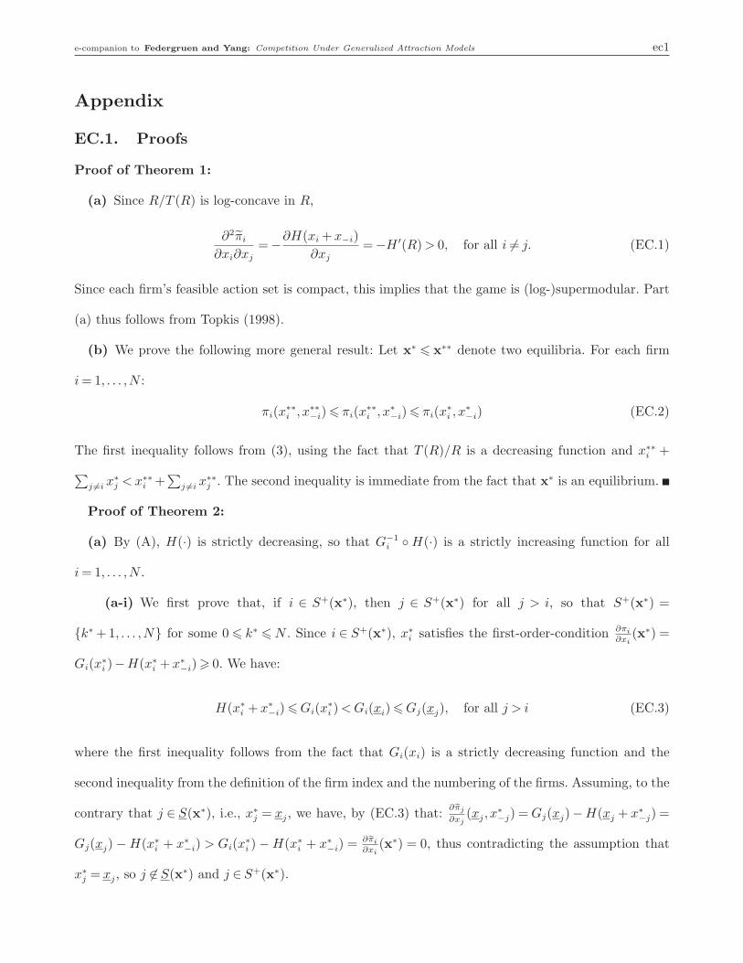
e-companion to Federgruen and Yang: Competition Under Generalized Attraction Models ec1
Appendix
EC.1. Proofs
Proof of Theorem 1:
(a) Since R/T (R) is log-concave in R,
∂2πi
∂xi∂xj
=−∂H(xi +x−i)
∂xj
=−H ′(R) > 0, for all i 6= j. (EC.1)
Since each firm’s feasible action set is compact, this implies that the game is (log-)supermodular. Part
(a) thus follows from Topkis (1998).
(b) We prove the following more general result: Let x∗ 6 x∗∗ denote two equilibria. For each firm
i = 1, . . . ,N :
πi(x∗∗i , x∗∗
−i) 6 πi(x∗∗i , x∗
−i) 6 πi(x∗i , x
∗−i) (EC.2)
The first inequality follows from (3), using the fact that T (R)/R is a decreasing function and x∗∗i +
∑j 6=i x
∗j < x∗∗
i +∑
j 6=i x∗∗j . The second inequality is immediate from the fact that x∗ is an equilibrium.
Proof of Theorem 2:
(a) By (A), H(·) is strictly decreasing, so that G−1i ◦ H(·) is a strictly increasing function for all
i = 1, . . . ,N .
(a-i) We first prove that, if i ∈ S+(x∗), then j ∈ S+(x∗) for all j > i, so that S+(x∗) =
{k∗ +1, . . . ,N} for some 0 6 k∗ 6 N . Since i ∈ S+(x∗), x∗i satisfies the first-order-condition ∂πi
∂xi(x∗) =
Gi(x∗i )−H(x∗
i +x∗−i) > 0. We have:
H(x∗i +x∗
−i) 6 Gi(x∗i ) < Gi(xi) 6 Gj(xj), for all j > i (EC.3)
where the first inequality follows from the fact that Gi(xi) is a strictly decreasing function and the
second inequality from the definition of the firm index and the numbering of the firms. Assuming, to the
contrary that j ∈ S(x∗), i.e., x∗j = xj, we have, by (EC.3) that:
∂eπj
∂xj(xj, x
∗−j) = Gj(xj)−H(xj + x∗
−j) =
Gj(xj) − H(x∗i + x∗
−i) > Gi(x∗i ) − H(x∗
i + x∗−i) = ∂eπi
∂xi(x∗) = 0, thus contradicting the assumption that
x∗j = xj, so j 6∈ S(x∗) and j ∈ S+(x∗).
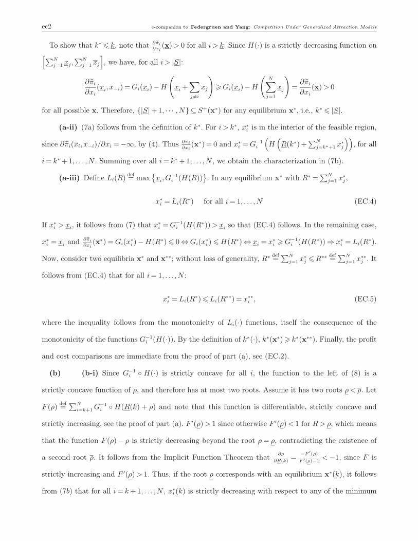
ec2 e-companion to Federgruen and Yang: Competition Under Generalized Attraction Models
To show that k∗ 6 k, note that ∂eπi
∂xi(x) > 0 for all i > k. Since H(·) is a strictly decreasing function on
[∑N
j=1 xj,∑N
j=1 xj
], we have, for all i > |S|:
∂πi
∂xi
(xi, x−i) = Gi(xi)−H
(xi +
∑
j 6=i
xj
)> Gi(xi)−H
(N∑
j=1
xj
)=
∂πi
∂xi
(x) > 0
for all possible x. Therefore, {|S|+1, · · · ,N} ⊆ S+(x∗) for any equilibrium x∗, i.e., k∗ 6 |S|.
(a-ii) (7a) follows from the definition of k∗. For i > k∗, x∗i is in the interior of the feasible region,
since ∂πi(xi, x−i)/∂xi =−∞, by (4). Thus ∂eπi
∂xi(x∗) = 0 and x∗
i = G−1i
(H(R(k∗)+
∑N
j=k∗+1 x∗j
)), for all
i = k∗ +1, . . . ,N . Summing over all i = k∗ +1, . . . ,N , we obtain the characterization in (7b).
(a-iii) Define Li(R)def= max
{xi,G
−1i (H(R))
}. In any equilibrium x∗ with R∗ =
∑N
j=1 x∗j ,
x∗i = Li(R
∗) for all i = 1, . . . ,N (EC.4)
If x∗i > xi, it follows from (7) that x∗
i = G−1i (H(R∗)) > xi so that (EC.4) follows. In the remaining case,
x∗i = xi and ∂eπi
∂xi(x∗) = Gi(x
∗i )−H(R∗) 6 0 ⇔ Gi(x
∗i ) 6 H(R∗) ⇔ xi = x∗
i > G−1i (H(R∗)) ⇒ x∗
i = Li(R∗).
Now, consider two equilibria x∗ and x∗∗; without loss of generality, R∗ def=∑N
j=1 x∗j 6 R∗∗ def
=∑N
j=1 x∗∗j . It
follows from (EC.4) that for all i = 1, . . . ,N :
x∗i = Li(R
∗) 6 Li(R∗∗) = x∗∗
i , (EC.5)
where the inequality follows from the monotonicity of Li(·) functions, itself the consequence of the
monotonicity of the functions G−1i (H(·)). By the definition of k∗(·), k∗(x∗) > k∗(x∗∗). Finally, the profit
and cost comparisons are immediate from the proof of part (a), see (EC.2).
(b) (b-i) Since G−1i ◦ H(·) is strictly concave for all i, the function to the left of (8) is a
strictly concave function of ρ, and therefore has at most two roots. Assume it has two roots ρ < ρ. Let
F (ρ)def=∑N
i=k+1 G−1i ◦ H(R(k) + ρ) and note that this function is differentiable, strictly concave and
strictly increasing, see the proof of part (a). F ′(ρ) > 1 since otherwise F ′(ρ) < 1 for R > ρ, which means
that the function F (ρ)− ρ is strictly decreasing beyond the root ρ = ρ, contradicting the existence of
a second root ρ. It follows from the Implicit Function Theorem that∂ρ
∂R(k)=
−F ′(ρ)
F ′(ρ)−1< −1, since F is
strictly increasing and F ′(ρ) > 1. Thus, if the root ρ corresponds with an equilibrium x∗(k), it follows
from (7b) that for all i = k + 1, . . . ,N , x∗i (k) is strictly decreasing with respect to any of the minimum
e-companion to Federgruen and Yang: Competition Under Generalized Attraction Models ec3
reliability standards, {x1, . . . , xk}, in particular, x1. Consider now the following restricted game in which
only firms k+1, . . . ,N compete, while the others are committed to operate at their minimum reliability
levels {x1, . . . , xk}. For firms i = k + 1, . . . ,N , replace xi by xi < x′i
def= x∗
i (k) < xi. In the restricted
game, each supplier’s action set continues to be given by a compact interval, and its log-profit functions
{πj : j = k +1, . . . ,N} are unaffected. Thus, the restricted game is supermodular as well. Since x∗(k) is
a Nash equilibrium in the original game, the vector[x∗
k+1(k), . . . , x∗N(k)
]is a Nash equilibrium in the
restricted game, now that the action sets of the players have shrunk. Moreover, as the lowest feasible
reliability vector in this game, it is clearly the smallest equilibrium. Since∂2eπj
∂xj∂x1> 0, see condition (A),
treating x1 as a parameter in the restricted game, it follows that each of the values[x∗
k+1(k), . . . , x∗N(k)
]
is increasing in x1, see Topkis (1998, Theorem 4.2.2), contradicting the fact that it is strictly decreasing
in x1. Thus, even if the characteristic equation has two roots, the lower root cannot correspond with
an equilibrium.
(b-ii) As shown in (b-i), the characteristic equation has at most two roots. The remaining char-
acterization of the equilibria with S(x∗) = ∅ follows directly from (7a) and (7b).
(b-iii) There are at most two equilibria with S(x∗) = ∅ by (b-ii) and at most one with S(x∗) =
{1, . . . , k} for k = 1, . . . , |S| by (b-i) and none for k = |S| + 1, . . . ,N by part (a-i). The number of
equilibria is thus bounded by |S|+2.
Proof of Theorem 3:
(a) The existence of an equilibrium follows from Theorem 1(a). It follows from Theorem 2(a-iii)
that the set of equilibria is completely ordered. This implies that all equilibria are symmetric. (If an
asymmetric equilibrium x∗ were to exist, every permutation of its components would be an equilibrium
as well, but could not be ordered with respect to x∗.)
(b) Since x > x0, we have for all x > x, ∂πi(x)/∂xi = G(xi)−H(∑N
j=1 xj
)< G(xi) 6 G(x0) = 0. (The
first inequality follows from H(·) being positive, as log(R/T (R)) is increasing; the second inequality
from G(·) being decreasing.) This implies that x is the unique equilibrium.
(c-i) Assume for a given number of firms, N , x is not an equilibrium. Thus, all equilibria are interior
and symmetric, by part (a). (The vector x is not an equilibrium, since ∂πi(x)/∂xi = G(x)−H(Nx) =
ec4 e-companion to Federgruen and Yang: Competition Under Generalized Attraction Models
−∞.) This implies that for any equilibrium (x∗, x∗, . . . , x∗), ∂πi(x∗)/∂xi = G(x∗) − H(Nx∗) = 0 ⇔
x∗ − G−1 ◦ H(Nx∗) = 0, so that the common component x∗ is a root of the characteristic equation.
Also, by condition (G), the characteristic equation has at most two roots. We now show that x∗ is the
larger (or unique) root. For all N = 2,3, . . ., let g(N)(ρ)def= G−1 ◦H((N − 1)x+ ρ)− ρ. Note first that
g( bN)(x) < 0 and θ( bN)(x) < 0 (EC.6)
(By the monotonicity of G(·), the first inequality is equivalent to H((N − 1)x + x) > G(x) = −∞; the
proof of the second inequality is identical.)
If θ( bN)(x) = g( bN)(x) > 0, it follows from the concavity of θ( bN)(·) and (EC.6) that θ( bN)(·) has a single
root on (x,x), so that the competition model has a single, symmetric and interior equilibrium, whose
common component is the unique root ρ(N) of the characteristic equation (9) on (x,x). Moreover, for
any N > N , g(N)(x) > g( bN)(x) > 0, which implies that ∂π(N)i (x,x−i)/∂xi > 0, which shows that x is not
an equilibrium in an industry with N > N firms, either. As shown above, it therefore has a unique,
symmetric and interior equilibrium, whose common component is the unique root, ρ(N) > ρ(N), of
θ(N)(·). (The fact that θ(N)(·) has a unique root follows from its concavity, θ(N)(x) > 0 and θ(N)(x) < 0;
the inequality ρ(N) > ρ(N) follows from the fact that θ(N)(·) is pointwise larger than θ( bN)(·).)
The remaining case has θ( bN)(x) = g( bN)(x) < 0. For this case, we first show that
Claim 1: If g( bN)(x) < 0, g( bN)(·) has two roots ρ(N) < ρ(N) on [x,x] and for all i = 1,2, . . . , N ,
πi(ρ(N),x−i) = maxx6ρ6x
πi(ρ,x−i) > πi(x). (EC.7)
Since g( bN)(·) is concave, g( bN)(x) < 0 and g( bN)(x) < 0, see (EC.6), g( bN)(·) has either zero or two roots
on [x,x]. However, in the former case, g( bN)(·) < 0 on the entire interval [x,x], and this inequality
implies 0 > ∂π( bN)i (ρ,x−i)/∂xi = G(ρ)−H((N − 1)x + ρ) for all ρ ∈ [x,x], again by composing it with
the monotone function G(·); this would imply that π( bN)i (x,x−i) = maxx6ρ6x π
( bN)i (ρ,x−i), contradicting
the fact that x is not an equilibrium. We conclude that g( bN)(·) has two roots ρ(N) < ρ(N) on [x,x]. By
the above arguments, for any firm i = 1,2, . . . , N : ∂π( bN)i (ρ,x−i)/∂xi < 0 except for ρ∈ [ρ(N), ρ(N)] , so
that only x and ρ(N) arise as local maxima of the function π( bN)i (·,x−i). The claim follows since x fails
to be an equilibrium.
e-companion to Federgruen and Yang: Competition Under Generalized Attraction Models ec5
Claim 2: If g( bN)(x) < 0, the function θ( bN)(·) has two roots ρ(N) < ρ(N), with ρ(N) 6 ρ(N) < ρ(N) 6
ρ(N).
This claim follows from the fact that θ( bN)(·) is concave, and pointwise larger than g( bN)(·) on (x,x),
θ( bN)(x) = g( bN)(x) < 0 and θ( bN)(x) < 0, by (EC.6). (The fact that θ( bN)(ρ) > g( bN)(ρ) for all ρ ∈ [x,x]
follows from (N −1)x+ρ 6 Nρ and the fact that the function G−1 ◦H is increasing as the composition
of two decreasing functions.)
It follows from Claim 1 that if all firms initially choose the lowest possible attraction value x, each firm
i’s best response is to move to ρ(N) > x. As mentioned in §3, the componentwise smallest equilibrium
x∗L(N) can be obtained by applying a simple tatonnement scheme, under which, starting with point x,
in each iteration, each firm determines its best response to the competitor’s choices. Moreover, it follows
from Theorems 4.3.2 and 4.3.4 in Topkis (1998) that this scheme generates an increasing sequence
of points which converge to x∗L(N). In particular, x < [ρ(N), . . . , ρ(N)] 6 x∗L(N). Since the common
component of x∗L(N) is a root the characteristic equation (9), it follows from Claim 2 that it equals
ρ(N) and that x∗L(N) = x∗H(N), i. e., the equilibrium is unique.
It remains to be shown that:
Claim 3: If g( bN)(x) < 0, for any N > N , x is not an equilibrium and ρ(N) > ρ(N).
If 0 < g(N)(x) = G−1 ◦ H(Nx) − x, it follows that 0 < ∂π(N)i (x,x−i)/∂xi = G(x) − H(Nx), which
implies that x fails to be an equilibrium in an industry with N firms. Moreover, since θ(N)(·) is concave,
while θ(N)(x) = g(N)(x) > 0 and θ(N)(x) < 0, it follows that θ(N)(·) has a unique root and ρ(N) > ρ(N),
where the inequality follows from the fact that θ(N)(·) is pointwise larger than θb(N)(·).
The remaining case has g(N)(x) 6 0, while by (EC.6), g(N)(x) < 0 as well. Note, however that g(N)(ρ) >
g( bN)(ρ) on the complete interval ρ ∈ [x,x], since G−1 ◦H, the composite of two decreasing functions,
is increasing; see (A). It follows that g(N)(·), just like g( bN)(·), has two roots ρ(N) < ρ(N) with ρ(N) >
ρ(N) > x. To complete the proof of the first part of Claim 3, by the above argument for an industry
with N firms, argmax π(N)i (·,x−i) = x or argmax π
(N)i (·,x−i) = ρ(N). However,
π(N)i (ρ(N),x−i)− π
(N)i (x,x−i) =
∫ bρ(N)
x
∂π(N)i (u,x−i)
∂xi
du =
∫ bρ( bN)
x
∂π(N)i (u,x−i)
∂xi
du +
∫ bρ(N)
bρ( bN)
∂π(N)i (u,x−i)
∂xi
du
ec6 e-companion to Federgruen and Yang: Competition Under Generalized Attraction Models
>
∫ bρ( bN)
x
∂π( bN)i (u,x−i)
∂xi
du = π( bN)i (ρ(N),x−i)− π
( bN)i (x,x−i) > 0 (EC.8)
(The first inequality follows from two facts: (i) for all u∈ [ρ(N), ρ(N)), 0 < ∂π(N)i (u,x−i)/∂u = G(u)−
H((N − 1)x + u) ⇔ 0 < G−1 ◦H((N − 1)x + u)−u = g(N)(u); (ii) For all u ∈ [x,x], ∂π(N)i (u,x−i)/∂u =
G(u)−H((N −1)x+u) > G(u)−H((N −1)x+u) = ∂π( bN)i (u,x−i)/∂u. The second inequality in (EC.8)
follows from Claim 1. Similar to the above proof that x∗L(N) > x, this implies that x∗L(N) > x as well.
In other words, x is not an equilibrium. Thus, if g(N)(x) 6 0, an industry with N firms, just like one with
N firms, has a unique equilibrium, whose common component is ρ(N). The inequality ρ(N) > ρ(N)
follows from the fact that θ(N)(·) is pointwise larger than θ( bN)(·).
Finally, we have shown that, if, for a given number of suppliers N , x is not an equilibrium, the same
must be true for all N > N . This implies the existence of an integer N 1(x) > N 0(x) > 2, such that x is
part of the equilibrium set for 2 6 N < N 0(x) and x is not an equilibrium for N > N 0. (N 0(x) 6 N 1(x),
since for N = N 1(x), ∂eπi(x)
∂xi= G−1 ◦H (N 1(x)x)−x > 0, so that x is not an equilibrium.)
(c-ii) Let N < N 0(x). Since all equilibria are symmetric, other than x, there may only be interior
symmetric equilibria x∗ = (x∗, . . . , x∗). For these, ∂eπi(x∗)
∂xi= G(x∗)−H(Nx∗) = 0⇔G−1 ◦H(Nx∗)−x∗ =
0, i.e., x∗ is one of the at most two roots (or solutions) of the concave function G−1 ◦ H(Nx) − x
(characteristic equation).
Proof of Lemma 1: Parts (a) and (b) follow from Theorem 5 and Lemma 1 of Federgruen and
Yang (2008a).
(c) We first show that f(R)def=√
µ2R +σ2(R− z2α)R is concave increasing in R.
f ′(R) =µ2 +σ2(2R− z2
α)
2f(R)> 0, since R > z2
α
f ′′(R) =4σ2f(R)− [µ2 +σ2(2R− z2
α)]2/f(R)
4f2(R)=
4σ2f2(R)− [µ2 +σ2(2R− z2α)]
2
4f3(R)
=−µ4 −σ4(2R− z2
α)2 − 2µ2σ2(2R− z2α)+ 4σ2µ2R +4σ4(R− z2
α)R
4f3(R)
=−µ4 −σ4z4
α +2µ2σ2z2α
4f3(R)=
− (µ2 −σ2z2α)
2
4f3(R)6 0
By (5),
H(R) = −{
log
[T (R)
R
]}′
= (logR)′ −{log [T (R)]}′
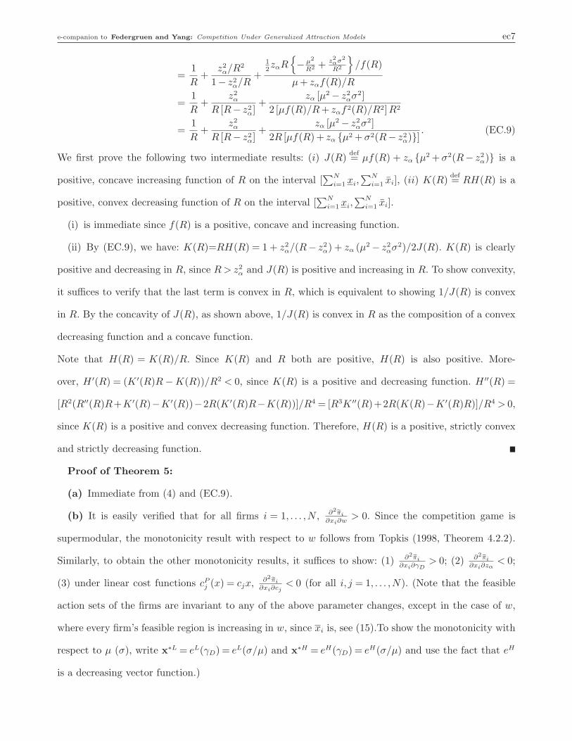
e-companion to Federgruen and Yang: Competition Under Generalized Attraction Models ec7
=1
R+
z2α/R2
1− z2α/R
+
12zαR
{− µ2
R2 + z2ασ2
R2
}/f(R)
µ+ zαf(R)/R
=1
R+
z2α
R [R− z2α]
+zα [µ2 − z2
ασ2]
2 [µf(R)/R + zαf2(R)/R2]R2
=1
R+
z2α
R [R− z2α]
+zα [µ2 − z2
ασ2]
2R [µf(R)+ zα {µ2 +σ2(R− z2α)}] . (EC.9)
We first prove the following two intermediate results: (i) J(R)def= µf(R) + zα {µ2 +σ2(R− z2
α)} is a
positive, concave increasing function of R on the interval [∑N
i=1 xi,∑N
i=1 xi], (ii) K(R)def= RH(R) is a
positive, convex decreasing function of R on the interval [∑N
i=1 xi,∑N
i=1 xi].
(i) is immediate since f(R) is a positive, concave and increasing function.
(ii) By (EC.9), we have: K(R)=RH(R) = 1 + z2α/(R− z2
α) + zα (µ2 − z2ασ2)/2J(R). K(R) is clearly
positive and decreasing in R, since R > z2α and J(R) is positive and increasing in R. To show convexity,
it suffices to verify that the last term is convex in R, which is equivalent to showing 1/J(R) is convex
in R. By the concavity of J(R), as shown above, 1/J(R) is convex in R as the composition of a convex
decreasing function and a concave function.
Note that H(R) = K(R)/R. Since K(R) and R both are positive, H(R) is also positive. More-
over, H ′(R) = (K ′(R)R − K(R))/R2 < 0, since K(R) is a positive and decreasing function. H ′′(R) =
[R2(R′′(R)R+K ′(R)−K ′(R))−2R(K ′(R)R−K(R))]/R4 = [R3K ′′(R)+2R(K(R)−K ′(R)R)]/R4 > 0,
since K(R) is a positive and convex decreasing function. Therefore, H(R) is a positive, strictly convex
and strictly decreasing function.
Proof of Theorem 5:
(a) Immediate from (4) and (EC.9).
(b) It is easily verified that for all firms i = 1, . . . ,N , ∂2eπi
∂xi∂w> 0. Since the competition game is
supermodular, the monotonicity result with respect to w follows from Topkis (1998, Theorem 4.2.2).
Similarly, to obtain the other monotonicity results, it suffices to show: (1) ∂2eπi
∂xi∂γD> 0; (2) ∂2eπi
∂xi∂zα< 0;
(3) under linear cost functions cPj (x) = cjx, ∂2eπi
∂xi∂cj< 0 (for all i, j = 1, . . . ,N). (Note that the feasible
action sets of the firms are invariant to any of the above parameter changes, except in the case of w,
where every firm’s feasible region is increasing in w, since xi is, see (15).To show the monotonicity with
respect to µ (σ), write x∗L = eL(γD) = eL(σ/µ) and x∗H = eH(γD) = eH(σ/µ) and use the fact that eH
is a decreasing vector function.)
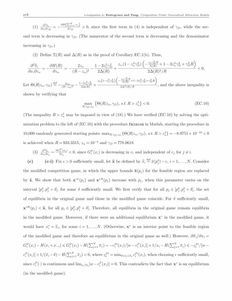
ec8 e-companion to Federgruen and Yang: Competition Under Generalized Attraction Models
(1) ∂2eπi
∂xi∂γD= −∂H(
PNj=1 xj)
∂γD> 0, since the first term in (4) is independent of γD, while the sec-
ond term is decreasing in γD. (The numerator of the second term is decreasing and the denominator
increasing in γD.)
(2) Define Σ(R) and ∆(R) as in the proof of Corollary EC.1(b). Thus,
∂2πi
∂xi∂zα
=−∂H(R)
∂zα
= − 2zα
(R− zα)2− 1− 3z2
αγ2D
2∆(R)+
zα (1− z2αγ2
D)(− zαγ2
DR
Σ(R)+1− 3z2
αγ2D + γ2
DR)
2∆(R)2/R< 0,
Let Θ(R|zα, γD)def= − 2zα
(R−zα)2− 1−3z2
αγ2D
2∆(R)+
zα(1−z2αγ2
D) −
zαγ2DR
Σ(R)+1−3z2
αγ2D+γ2
DR
!
2∆2(R)/R, and the above inequality is
shown by verifying that
maxR,γD,zα
{Θ(R|zα, γD), s.t. R > z2
α
}< 0. (EC.10)
(The inequality R > z2α may be imposed in view of (18).) We have verified (EC.10) by solving the opti-
mization problem to the left of (EC.10) with the procedure fmincon in Matlab, starting the procedure in
10,000 randomly generated starting points: maxR,γD,zα {Θ(R|zα, γD), s.t. R > z2α}=−8.9751×10⁻¹⁰ < 0
is achieved when R = 933.3315, zα = 10−4 and γD = 778.0618.
(3) ∂2eπi
∂xi∂cj=
∂GPi (xi)
∂cj< 0, since GP
i (xi) is decreasing in ci and independent of cj for j 6= i.
(c) (c-i) Fix ǫ > 0 sufficiently small, let x be defined by xidef= x(p0
j)− ǫ, i = 1, . . . ,N . Consider
the modified competition game, in which the upper bounds x(pj) for the feasible region are replaced
by x. We show that both x∗L(pj) and x∗H(pj) increase with pj, when this parameter varies on the
interval [p0j , p
0j + δ], for some δ sufficiently small. We first verify that for all pj ∈ [p0
j , p0j + δ], the set
of equilibria in the original game and those in the modified game coincide. For δ sufficiently small,
x∗H(pj) < x, for all pj ∈ [p0j , p
0j + δ]. Therefore, all equilibria in the original game remain equilibria
in the modified game. Moreover, if there were an additional equilibrium x∗ in the modified game, it
would have x∗i = xi, for some i = 1, . . . ,N . (Otherwise, x∗ is an interior point to the feasible region
of the modified game and therefore an equilibrium in the original game as well.) However, ∂πi/∂xi =
GPi (xi)−H(xi +x−i) 6 GP
i (xi)−H(∑N
j=1 xj) =−cP ′i (xi)/[w− cP
i (xi)]+1/xi −H(∑N
j=1 xj) 6−cP ′i /[w−
cPi (xi)]+1/(xi−δ)−H(
∑N
j=1 xj) < 0, where cP ′i = min06xi6xi
cP ′i (xi), when choosing ǫ sufficiently small,
since cPi (·) is continuous and limxi↑xi
[w−cPi (xi)] = 0. This contradicts the fact that x∗ is an equilibrium
(in the modified game).
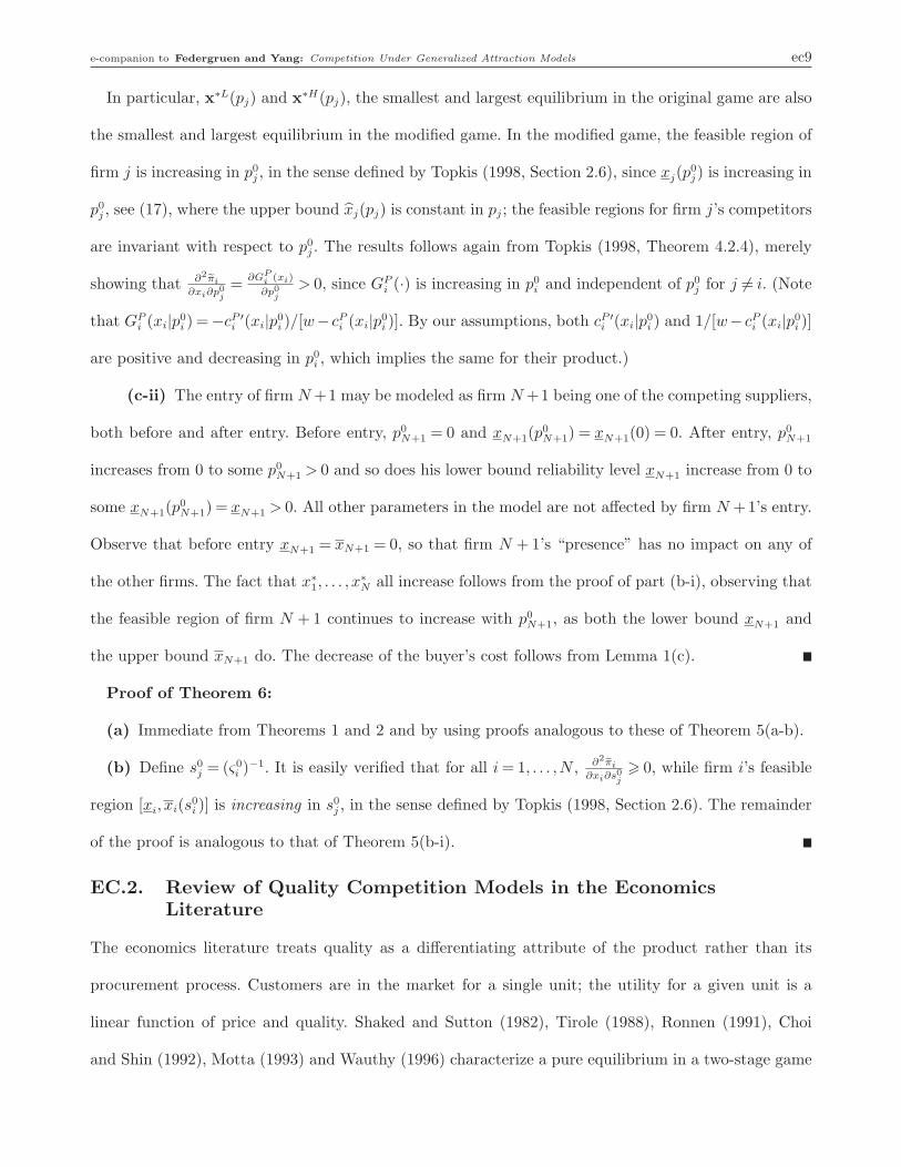
e-companion to Federgruen and Yang: Competition Under Generalized Attraction Models ec9
In particular, x∗L(pj) and x∗H(pj), the smallest and largest equilibrium in the original game are also
the smallest and largest equilibrium in the modified game. In the modified game, the feasible region of
firm j is increasing in p0j , in the sense defined by Topkis (1998, Section 2.6), since xj(p
0j) is increasing in
p0j , see (17), where the upper bound xj(pj) is constant in pj; the feasible regions for firm j’s competitors
are invariant with respect to p0j . The results follows again from Topkis (1998, Theorem 4.2.4), merely
showing that ∂2eπi
∂xi∂p0j
=∂GP
i (xi)
∂p0j
> 0, since GPi (·) is increasing in p0
i and independent of p0j for j 6= i. (Note
that GPi (xi|p0
i ) =−cP ′i (xi|p0
i )/[w− cPi (xi|p0
i )]. By our assumptions, both cP ′i (xi|p0
i ) and 1/[w− cPi (xi|p0
i )]
are positive and decreasing in p0i , which implies the same for their product.)
(c-ii) The entry of firm N +1 may be modeled as firm N +1 being one of the competing suppliers,
both before and after entry. Before entry, p0N+1 = 0 and xN+1(p
0N+1) = xN+1(0) = 0. After entry, p0
N+1
increases from 0 to some p0N+1 > 0 and so does his lower bound reliability level xN+1 increase from 0 to
some xN+1(p0N+1) = xN+1 > 0. All other parameters in the model are not affected by firm N +1’s entry.
Observe that before entry xN+1 = xN+1 = 0, so that firm N + 1’s “presence” has no impact on any of
the other firms. The fact that x∗1, . . . , x
∗N all increase follows from the proof of part (b-i), observing that
the feasible region of firm N + 1 continues to increase with p0N+1, as both the lower bound xN+1 and
the upper bound xN+1 do. The decrease of the buyer’s cost follows from Lemma 1(c).
Proof of Theorem 6:
(a) Immediate from Theorems 1 and 2 and by using proofs analogous to these of Theorem 5(a-b).
(b) Define s0j = (ς0
i )−1. It is easily verified that for all i = 1, . . . ,N , ∂2eπi
∂xi∂s0j
> 0, while firm i’s feasible
region [xi, xi(s0i )] is increasing in s0
j , in the sense defined by Topkis (1998, Section 2.6). The remainder
of the proof is analogous to that of Theorem 5(b-i).
EC.2. Review of Quality Competition Models in the EconomicsLiterature
The economics literature treats quality as a differentiating attribute of the product rather than its
procurement process. Customers are in the market for a single unit; the utility for a given unit is a
linear function of price and quality. Shaked and Sutton (1982), Tirole (1988), Ronnen (1991), Choi
and Shin (1992), Motta (1993) and Wauthy (1996) characterize a pure equilibrium in a two-stage game
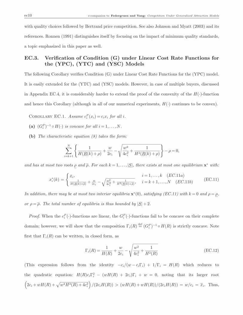
ec10 e-companion to Federgruen and Yang: Competition Under Generalized Attraction Models
with quality choices followed by Bertrand price competition. See also Johnson and Myatt (2003) and its
references. Ronnen (1991) distinguishes itself by focusing on the impact of minimum quality standards,
a topic emphasized in this paper as well.
EC.3. Verification of Condition (G) under Linear Cost Rate Functions forthe (YPC), (YTC) and (YSC) Models
The following Corollary verifies Condition (G) under Linear Cost Rate Functions for the (YPC) model.
It is easily extended for the (YTC) and (YSC) models. However, in case of multiple buyers, discussed
in Appendix EC.4, it is considerably harder to extend the proof of the convexity of the H(·)-function
and hence this Corollary (although in all of our numerical experiments, H(·) continues to be convex).
Corollary EC.1. Assume cPi (xi) = cixi for all i.
(a) (GPi )−1 ◦H(·) is concave for all i = 1, . . . ,N .
(b) The characteristic equation (8) takes the form:
N∑
i=k+1
{1
H(R(k)+ ρ)+
w
2ci
−√
w2
4c2i
+1
H2(R(k)+ ρ)
}− ρ = 0,
and has at most two roots ρ and ρ. For each k = 1, . . . , |S|, there exists at most one equilibrium x∗ with:
x∗i (k) =
{xi, i = 1, . . . , k (EC.11a)
1H(R(k)+ρ)
+ w2ci
−√
w2
4c2i
+ 1H2(R(k)+ρ)
, i = k +1, . . . ,N (EC.11b)(EC.11)
In addition, there may be at most two interior equilibria x∗(0), satisfying (EC.11) with k = 0 and ρ = ρ,
or ρ = ρ. The total number of equilibria is thus bounded by |S|+2.
Proof. When the cPi (·)-functions are linear, the GP
i (·)-functions fail to be concave on their complete
domain; however, we will show that the composition Γi(R)def= (GP
i )−1 ◦H(R) is strictly concave. Note
first that Γi(R) can be written, in closed form, as
Γi(R) =1
H(R)+
w
2ci
−√
w2
4c2i
+1
H2(R)(EC.12)
(This expression follows from the identity −ci/(w− ciΓi) + 1/Γi = H(R) which reduces to
the quadratic equation: H(R)ciΓ2i − (wH(R) + 2ci)Γi + w = 0, noting that its larger root
(2ci +wH(R)+
√w2H2(R)+ 4c2
i
)/(2ciH(R)) > (wH(R)+wH(R))/(2ciH(R)) = w/ci = xi. Thus,
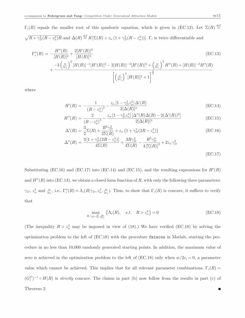
e-companion to Federgruen and Yang: Competition Under Generalized Attraction Models ec11
Γi(R) equals the smaller root of this quadratic equation, which is given in (EC.12). Let Σ(R)def=
√R + γ2
D(R− z2α)R and ∆(R)
def= R [Σ(R)+ zα (1+ γ2
D(R− z2α))]. Γi is twice differentiable and
Γ′′i (R) = − H ′′(R)
[H(R)]2+
2[H ′(R)]2
[H(R)]3(EC.13)
+−3(
w2ci
)2
[H(R)]−1[H ′(R)]2 − 2[H(R)]−3[H ′(R)]2 +(
w2ci
)2
H ′′(R)+ [H(R)]−2H ′′(R)
[(w2ci
)2
[H(R)]2 +1
] 32
where
H ′(R) = − 1
(R− z2α)
2 −zα [1− γ2
Dz2α]∆′(R)
2[∆(R)]2(EC.14)
H ′′(R) =2
(R− z2α)
3 − zα [1− γ2Dz2
α] [∆′′(R)∆(R)− 2(∆′(R))2]
2[∆(R)]3(EC.15)
∆′(R) =3
2Σ(R)+
R2γ2D
2Σ(R)+ zα
(1+ γ2
D(2R− z2α))
(EC.16)
∆′′(R) =3 [1+ γ2
D(2R− z2α)]
4Σ(R)+
3Rγ2D
4Σ(R)− R3γ4
D
4 [Σ(R)]3 +2zαγ2
D
(EC.17)
Substituting (EC.16) and (EC.17) into (EC.14) and (EC.15), and the resulting expressions for H ′(R)
and H ′′(R) into (EC.13), we obtain a closed form function of R, with only the following three parameters:
γD, z2α and w
2ci, i.e., Γ′′
i (R) = Λi(R|γD, z2α, w
2ci). Thus, to show that Γi(R) is concave, it suffices to verify
that
maxR,γD,z2
α, w2ci
{Λi(R), s.t. R > z2
α
}= 0 (EC.18)
(The inequality R > z2α may be imposed in view of (18).) We have verified (EC.18) by solving the
optimization problem to the left of (EC.18) with the procedure fmincon in Matlab, starting the pro-
cedure in no less than 10,000 randomly generated starting points. In addition, the maximum value of
zero is achieved in the optimization problem to the left of (EC.18) only when w/2ci = 0, a parameter
value which cannot be achieved. This implies that for all relevant parameter combinations, Γi(R) =
(GPi )−1 ◦ H(R) is strictly concave. The claims in part (b) now follow from the results in part (c) of
Theorem 2.
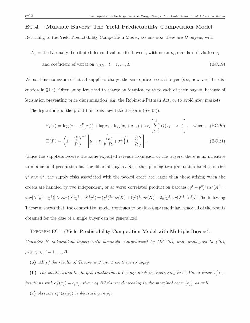
ec12 e-companion to Federgruen and Yang: Competition Under Generalized Attraction Models
EC.4. Multiple Buyers: The Yield Predictability Competition Model
Returning to the Yield Predictability Competition Model, assume now there are B buyers, with
Dl = the Normally distributed demand volume for buyer l, with mean µl, standard deviation σl
and coefficient of variation γD,l, l = 1, . . . ,B (EC.19)
We continue to assume that all suppliers charge the same price to each buyer (see, however, the dis-
cussion in §4.4). Often, suppliers need to charge an identical price to each of their buyers, because of
legislation preventing price discrimination, e.g. the Robinson-Patman Act, or to avoid grey markets.
The logarithms of the profit functions now take the form (see (3)):
πi(x) = log(w− cP
i (xi))+ logxi − log (xi +x−i)+ log
[B∑
l=1
Tl (xi +x−i)
], where (EC.20)
Tl(R) =
(1− z2
α
R
)−1[µl + zα
õ2
l
R+σ2
l
(1− z2
α
R
)]. (EC.21)
(Since the suppliers receive the same expected revenue from each of the buyers, there is no incentive
to mix or pool production lots for different buyers. Note that pooling two production batches of size
y1 and y2, the supply risks associated with the pooled order are larger than those arising when the
orders are handled by two independent, or at worst correlated production batches:(y1 + y2)2var(X) =
var[X(y1 + y2)] > var(X1y1 + X2y2) = (y1)2var(X) + (y2)2var(X) + 2y1y2cov(X1,X2).) The following
Theorem shows that, the competition model continues to be (log-)supermodular, hence all of the results
obtained for the case of a single buyer can be generalized.
Theorem EC.1 (Yield Predictability Competition Model with Multiple Buyers).
Consider B independent buyers with demands characterized by (EC.19), and, analogous to (10),
µl > zασl, l = 1, . . . ,B.
(a) All of the results of Theorems 2 and 3 continue to apply.
(b) The smallest and the largest equilibrium are componentwise increasing in w. Under linear cPj (·)-
functions with cPj (xj) = cjxj, these equilibria are decreasing in the marginal costs {cj} as well.
(c) Assume cP ′i (xi|p0
i ) is decreasing in p0i .
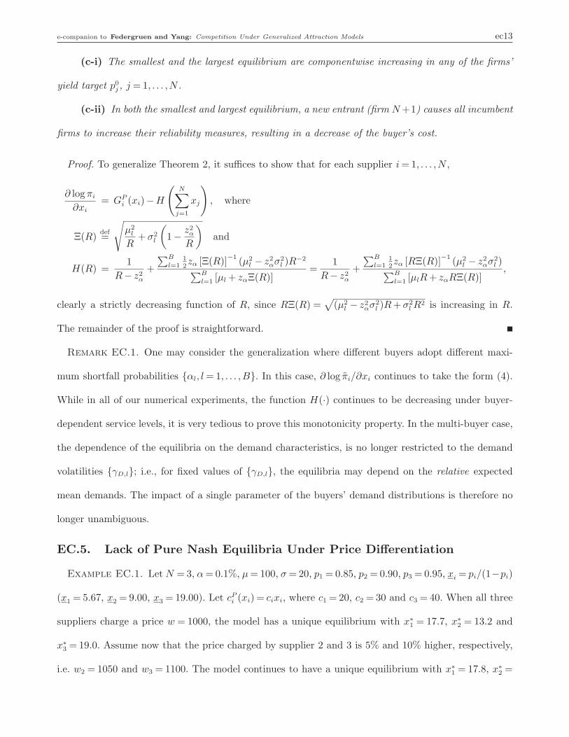
e-companion to Federgruen and Yang: Competition Under Generalized Attraction Models ec13
(c-i) The smallest and the largest equilibrium are componentwise increasing in any of the firms’
yield target p0j , j = 1, . . . ,N .
(c-ii) In both the smallest and largest equilibrium, a new entrant (firm N +1) causes all incumbent
firms to increase their reliability measures, resulting in a decrease of the buyer’s cost.
Proof. To generalize Theorem 2, it suffices to show that for each supplier i = 1, . . . ,N ,
∂ logπi
∂xi
= GPi (xi)−H
(N∑
j=1
xj
), where
Ξ(R)def=
õ2
l
R+σ2
l
(1− z2
α
R
)and
H(R) =1
R− z2α
+
∑B
l=112zα [Ξ(R)]
−1(µ2
l − z2ασ2
l )R−2
∑B
l=1 [µl + zαΞ(R)]=
1
R− z2α
+
∑B
l=112zα [RΞ(R)]
−1(µ2
l − z2ασ2
l )∑B
l=1 [µlR + zαRΞ(R)],
clearly a strictly decreasing function of R, since RΞ(R) =√
(µ2l − z2
ασ2l )R +σ2
l R2 is increasing in R.
The remainder of the proof is straightforward.
Remark EC.1. One may consider the generalization where different buyers adopt different maxi-
mum shortfall probabilities {αl, l = 1, . . . ,B}. In this case, ∂ log πi/∂xi continues to take the form (4).
While in all of our numerical experiments, the function H(·) continues to be decreasing under buyer-
dependent service levels, it is very tedious to prove this monotonicity property. In the multi-buyer case,
the dependence of the equilibria on the demand characteristics, is no longer restricted to the demand
volatilities {γD,l}; i.e., for fixed values of {γD,l}, the equilibria may depend on the relative expected
mean demands. The impact of a single parameter of the buyers’ demand distributions is therefore no
longer unambiguous.
EC.5. Lack of Pure Nash Equilibria Under Price Differentiation
Example EC.1. Let N = 3, α = 0.1%, µ = 100, σ = 20, p1 = 0.85, p2 = 0.90, p3 = 0.95, xi = pi/(1−pi)
(x1 = 5.67, x2 = 9.00, x3 = 19.00). Let cPi (xi) = cixi, where c1 = 20, c2 = 30 and c3 = 40. When all three
suppliers charge a price w = 1000, the model has a unique equilibrium with x∗1 = 17.7, x∗
2 = 13.2 and
x∗3 = 19.0. Assume now that the price charged by supplier 2 and 3 is 5% and 10% higher, respectively,
i.e. w2 = 1050 and w3 = 1100. The model continues to have a unique equilibrium with x∗1 = 17.8, x∗
2 =
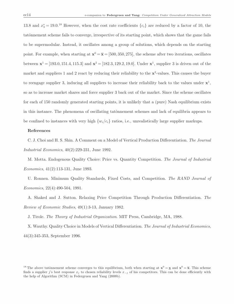
ec14 e-companion to Federgruen and Yang: Competition Under Generalized Attraction Models
13.8 and x∗3 = 19.0.18 However, when the cost rate coefficients {ci} are reduced by a factor of 10, the
tatonnement scheme fails to converge, irrespective of its starting point, which shows that the game fails
to be supermodular. Instead, it oscillates among a group of solutions, which depends on the starting
point. For example, when starting at x0 = x = [500,350,275], the scheme after two iterations, oscillates
between x1 = [193.0,151.4,115.3] and x2 = [182.3,129.2,19.0]. Under x1, supplier 3 is driven out of the
market and suppliers 1 and 2 react by reducing their reliability to the x2-values. This causes the buyer
to reengage supplier 3, inducing all suppliers to increase their reliability back to the values under x1,
so as to increase market shares and force supplier 3 back out of the market. Since the scheme oscillates
for each of 150 randomly generated starting points, it is unlikely that a (pure) Nash equilibrium exists
in this instance. The phenomena of oscillating tatonnement schemes and lack of equilibria appears to
be confined to instances with very high {wi/ci} ratios, i.e., unrealistically large supplier markups.
References
C. J. Choi and H. S. Shin. A Comment on a Model of Vertical Production Differentiation. The Journal
Industrial Economics, 40(2):229-231, June 1992.
M. Motta. Endogenous Quality Choice: Price vs. Quantity Competition. The Journal of Industrial
Economics, 41(2):113-131, June 1993.
U. Ronnen. Minimum Quality Standards, Fixed Costs, and Competition. The RAND Journal of
Economics, 22(4):490-504, 1991.
A. Shaked and J. Sutton. Relaxing Price Competition Through Production Differentiation. The
Review of Economic Studies, 49(1):3-13, January 1982.
J. Tirole. The Theory of Industrial Organization. MIT Press, Cambridge, MA, 1988.
X. Wauthy. Quality Choice in Models of Vertical Differentiation. The Journal of Industrial Economics,
44(3):345-353, September 1996.
18 The above tatonnement scheme converges to this equilibrium, both when starting at x0 = x and x
0 = x. This schemefinds a supplier j’s best response xj to chosen reliability levels x−j of his competitors. This can be done efficiently withthe help of Algorithm (SCM) in Federgruen and Yang (2008b).

![DYNAMICAL BEHAVIORS OF ATTRACTION …...2020/04/01 · chemotaxis model (1) has been generalized to simulate the biological or medical phenomena [24], such as the bacteria aggregation](https://img.pdfslide.us/doc/110x75/5fbea4db95e6fc337a1c6e85/dynamical-behaviors-of-attraction-20200401-chemotaxis-model-1-has-been.jpg)


![Understanding the Law of Attraction - 2nd Law of Attraction [Bootcamp]](https://img.pdfslide.us/doc/110x75/58ecbcb91a28ab44238b460f/understanding-the-law-of-attraction-2nd-law-of-attraction-bootcamp.jpg)