Competition, Markups,and the Gains from International Trade∗

Chris Edmond† Virgiliu Midrigan‡ Daniel Yi Xu§

November 2011

Abstract

We study product-level data for Taiwanese manufacturing establishments through

the lens of a model with endogenously variable markups. We find that the gains from

international trade can be large: in our benchmark model, moving from autarky to a

10% import share implies an increase in welfare equivalent to a 27% permanent increase

in consumption. By contrast, a standard trade model with constant markups implies a

smaller gain, around a 4% increase in consumption. By increasing competition, trade

reduces markups and so reduces distortions in labor and investment choices. Greater

competition also induces a more efficient allocation of factors of production across es-

tablishments, thereby directly raising TFP. These channels are an order of magnitude

more important than the love-of-variety effects in standard trade models. Our model

predicts that industries that are more open are characterized by lower revenue produc-

tivity and lower dispersion in revenue productivity across producers. We find strong

support for these predictions of the model in the Taiwanese data. In our model, mi-

cro details such as as the dispersion of industry-level import shares determine how the

Armington elasticity endogenously responds to a change in trade policy. Consequently,

these micro details also matter for determining the size of the gains from standard

love-of-variety effects.

Keywords: market shares, productivity, misallocation, welfare, Armington elasticity.

JEL classifications: F1, O4.

∗We thank Fernando Alvarez, Ariel Burstein, Jan De Loecker, Phil McCalman, Barbara Spencer and sem-inar participants at UBC, University of Chicago (Booth), Deakin University, Monash University, Wharton,the 2011 NBER Macroeconomics and Productivity meeting, and the 2011 SED annual meeting.†University of Melbourne, cedmond@unimelb.edu.au.‡Federal Reserve Bank of Minneapolis, New York University, and NBER, virgiliu.midrigan@nyu.edu.§Duke University, New York University, and NBER, daniel.xu@duke.edu.

1 Introduction

How large are the welfare gains from international trade? We answer this question using a

quantitative model with endogenously variable markups. Our main finding is that the welfare

gains from trade can be large and, in particular, can be an order of magnitude larger than

those implied by standard models with markups that do not change in response to trade.

In our model, opening an economy to trade exposes domestic firms to a pro-competitive

mechanism which reduces market shares and increases demand elasticity. As a consequence,

firms charge smaller markups over marginal cost. The impact of increased competition on

markups leads to gains from trade both by reducing average markups and by reducing dis-

persion in markups. The former effect directly reduces distortions in labor and investment

decisions. The latter effect promotes a more efficient allocation of factors across estab-

lishments and so increases total factor productivity (TFP). We quantify the model using

product-level data for Taiwanese manufacturing establishments and find that both markup

effects can be substantial. Combined, the model predicts that moving from autarky to a

10% import share implies an increase in welfare equivalent to a 27% permanent increase in

consumption. By contrast, a standard trade model that does not account for the effects of

increased competition on markups would predict a 4% increase in consumption.

We are far from the first to argue that the pro-competitive effects of trade may increase

productivity and welfare. Instead, our main contribution is to carefully quantify the pro-

competitive mechanism. To conduct this exercise we use a model developed by Devereux

and Lee (2001) and Atkeson and Burstein (2008). The model features a nested pair of

constant elasticity demand systems. Within a country, there is a continuum of imperfectly

substitutable industries. Within any given industry, there is a small number of firms who

engage in oligopolistic competition and whose products are more substitutable for one another

than they are substitutable for products from other industries. The demand elasticity for any

given firm depends on both these margins of substitution and on that firm’s market share

in its industry. A firm that is a monopolist in its industry faces no competition from close

substitutes and so faces a less elastic demand curve than a firm that has a low market share.

In this model, the market shares of firms, and hence their demand elasticities and markups,

are determined in equilibrium. Heterogeneity in market shares is driven by exogenous firm-

level productivity differences.

We consider a world with two perfectly symmetric countries.1 A firm in either country

can sell into its industry abroad, thereby exposing firms in that industry abroad to more

1By considering perfectly symmetric countries — and thus abstracting from aggregate differences in factorendowments or technologies — we isolate the gains from trade that are exclusively due to intraindustry trade,as in Krugman (1979, 1980).

1

competition, but to do so incurs an iceberg trade cost. Our main interest is the welfare gains

from increased exposure to trade that result from reductions in tariffs on importers.2 For

intuition, consider an industry consisting of one large firm that has a high market share and

charges a high markup plus a small number of less productive firms that have low market

shares and charge low markups. This industry will have a high (revenue-weighted) average

markup but also a considerable amount of markup dispersion between the large firm and the

small firms. Now imagine confronting this industry with competition from symmetric firms

in the same industry abroad. The increased competition will reduce market power across

the board, driving down the market share of the large firm (in each country) and thereby

increasing demand elasticities and reducing markups. This increase in competition brought

about by opening to trade both reduces the average markup and, by shifting the large firms

out of the tails of the markup distribution, also reduces dispersion in markups.

To quantify the effect of more competition on markups, we use product-level (7-digit)

Taiwanese manufacturing data. We combine this with import data from the WTO to obtain

disaggregated import shares for each product category. We use this data to discipline three

key factors governing the size of the gains from trade in our model: (i) the equilibrium dis-

tribution of firm-level market shares, (ii) the extent to which substitution across industries is

a good alternative to substitution within an industry, and (iii) the equilibrium magnitude of

the Armington elasticity, i.e., the sensitivity of trade flows to changes in trade costs. In par-

ticular, we pin down the parameters governing the firm-level distribution of productivity and

fixed costs of operating and exporting by requiring the model to reproduce the distribution

of market shares and industry concentration statistics in the Taiwanese data. We choose the

elasticity of substitution within industries so that our model matches standard estimates of

the Armington elasticity. We choose the elasticity of substitution between industries so that

our model fits the cross-sectional relationship between labor shares and market shares that

we observe in the Taiwanese data. All other parameters are assigned values consistent with

those used in existing work.

Our benchmark model predicts large gains from trade through the effect that increased

competition has on the distribution of markups. First, holding fixed a given level of aggregate

TFP, increased trade reduces the aggregate markup and so reduces distortions in labor and

investment decisions. Second, holding fixed a given level of the aggregate markup, increased

trade reduces the dispersion in markups and so endogenously increases the level of aggregate

TFP as factors of production are more efficiently allocated. We find that both these effects

are large. For example, going from our benchmark economy to the first-best (i.e., eliminating

2We interpret the trade costs in our model as being essentially technological, at least in the sense of theirbeing difficult to change with policy. Accordingly, we find it more natural to compute the welfare implicationsof changes in the level of taxes/subsidies on importers.

2

both the level and dispersion in markups) gives a welfare gain equivalent to a 17% perma-

nent rise in consumption. Of this, a 6.5% welfare gain can be obtained by eliminating the

dispersion in markups while leaving the aggregate markup unchanged at its benchmark level.

Thus in this case both effects play a substantial role in delivering the overall welfare gains.

Increasing TFP by reducing markup dispersion is an effect familiar from the work on

“misallocation” of factors of production by Restuccia and Rogerson (2008), Hsieh and Klenow

(2009) and others. We find that international trade can play a powerful role in reducing

misallocation and so increase productivity both at home and abroad. In short, the size of the

welfare gains from trade and the extent to which misallocation suppresses the level of TFP are

closely related concerns. From a policy point of view, our model suggests that obtaining large

welfare gains from an improved allocation may not require the detailed, perhaps impractical,

scheme of cross-subsidies/taxes that implement the first-best. Instead, simply opening an

economy to trade may provide an excellent practical alternative that substantially improves

welfare even if it does not go all the way to the first-best.

Beginning with Eaton and Kortum (2002) and Melitz (2003), a large recent literature on

trade with heterogeneous firms has emphasized two conceptually distinct but related channels

by which trade may lead to welfare gains. The first channel is a selection effect. Exposure to

trade forces less productive firms to exit and the resulting reallocation of resources increases

measured productivity, as in the empirical work of Aw, Chung and Roberts (2000), Pavcnik

(2002) and others. Selection is driven by the need to cover fixed costs of operating and/or

exporting. In other words, this channel of reallocation operates at the extensive margin.

Without the exit of less productive firms, there would be no increase in aggregate productiv-

ity. And as emphasized by Arkolakis, Costinot and Rodrıguez-Clare (2011), the quantitative

gains from trade in any reasonably calibrated version of a model of this kind are small. The

second channel is the pro-competitive effect that we focus on. Reallocation in our model

occurs primarily at the intensive margin and there are quantitatively significant gains from

trade even if there is no exit by less productive firms.3 Almost all the gains from trade in

our model come from reallocation due to changes in the distribution of markups.4

In models such as Melitz (2003), trade has only a selection effect and has no pro-

competitive effect because markups are constant. In other trade models, the absence of

pro-competitive effects occurs for more subtle reasons. For example, in Bernard, Eaton,

Jensen and Kortum (2003) — BEJK hereafter — heterogeneous firms compete in Bertrand

fashion to be the sole producer in their industry, and this indeed gives rise to an endogenous

3In our model, trade acts like the competitive pressure effects surveyed in Holmes and Schmitz (2010).4Our model includes fixed costs of operating and exporting and so also features reallocation due to

selection, but these effects are quantitatively small. We include fixed costs only to ensure that the model canbetter match the micro-data we use to determine our key parameters.

3

markup distribution. The properties of this distribution depend on whether the lowest cost

and second-lowest cost firms are domestic or foreign and, in principle, the effects of increased

trade depend on how (if at all) trade leads to a new configuration of lowest and second-

lowest cost firms. But owing to special properties of the Frechet distribution, which BEJK

use to model firm-level productivity draws, it can be shown that the markup distribution is

invariant to a trade liberalization. Increased trade reduces prices but also proportionately

reduces costs so that markups are unchanged. Consequently, this analysis misses the effect

of trade-induced changes in competition on markups and TFP.

A pro-competitive effect in a model of imperfect competition can be obtained by de-

parting from the assumption of a large number of firms facing constant elasticity demand.

Brander (1981) and Brander and Krugman (1983) provide examples of this using models

of Cournot competition in partial equilibrium settings. More recently, Devereux and Lee

(2001) and Atkeson and Burstein (2008) have considered dynamic general equilibrium trade

models featuring competition between a small number of firms facing constant elasticity de-

mand. Melitz and Ottaviano (2008) consider monopolistic competition by a large number

of firms that face linear demand curves and hence a variable elasticity of demand. Both

of these frameworks predict that more productive firms will have larger market shares and

charge larger markups. In both frameworks, an increase in international trade has the effect

of increasing competition and reducing markups.5 Other departures from constant elastic-

ity demand, such as the translog demand systems considered by Feenstra and Weinstein

(2010) and Novy (2010) can give similar effects.6 In addition to its theoretical appeal, this

pro-competitive effect is widely documented in empirical work. Examples from the trade lit-

erature include Harrison (1994), Levinsohn (1993), Krishna and Mitra (1998), and Bottasso

and Sembenelli (2001). Campbell and Hopenhayn (2005) document a similar effect in U.S.

establishment data. Relative to this empirical work, our main contribution is to embed the

pro-competitive mechanism in a tightly grounded model that can be used for welfare analysis

and counterfactual experiments.

Several recent theoretical papers on variable markups also highlight the importance of

changes in markup dispersion for aggregate productivity and the gains from trade. Epi-

fani and Gancia (2011) provide conditions under which falls in markup dispersion increase

5In Devereux and Lee (2001), as in the original Dixit and Stiglitz (1977) model, the markup is endoge-nous to the number of producers but the distribution of market shares is uniform. Atkeson and Burstein(2008) extend this model by considering firm-level heterogeneity in productivity which then determines, inequilibrium, the distribution of market shares.

6Arkolakis, Costinot and Rodrıguez-Clare (2010) show, however, that if firm-level productivity has aPareto distribution then the translog demand system will still give small gains from trade. The intuition forthis is that with free-entry, the markup is pinned down by the fixed cost of entry and the threat of furtherentry already provides enough competition that competition from international firms has little extra effect.

4

aggregate productivity, but in their analysis the markup distribution is exogenous. Peters

(2011) provides a related analysis of a closed-economy model where the markup distribution

is endogenous because of entry/exit decisions by firms and discusses the implications of the

markup distribution for aggregate productivity. Like us, he emphasizes that only the aggre-

gate markup matters for factor prices, and hence for labor and investment decisions, and that

it is markup dispersion that inefficiently reduces aggregate productivity. De Blas and Russ

(2010) have extended BEJK so that the distribution of markups is endogenous to trade costs.

Holmes, Hsu and Lee (2011) make a related theoretical contribution and construct a model

that nests both a standard constant elasticity framework and BEJK framework as special

cases. Though they differ in details, both Holmes et al. (2011) and De Blas and Russ (2010)

have a selection effect and a pro-competitive effect and both can account, qualitatively, for a

trade-induced fall in markup dispersion and the resulting increase in productivity. Relative

to these papers, our main contribution is quantifying the pro-competitive mechanism.

To further evaluate the pro-competitive mechanism, we examine several other predictions

of the model. For example, the model predicts that industries with higher import shares

are more competitive and have both lower levels of measured revenue (labor) productivity

and lower dispersion in revenue productivity. Encouragingly for our mechanism, we find

strong support for both predictions in the Taiwanese data. We find that industries with

high import shares have substantially lower average revenue productivity and substantially

lower dispersion in revenue productivity. Both relationships hold even when we control for

differences in capital intensity at the industry level. Moreover, we find that most of the

reduction in dispersion comes from reducing the revenue productivity of the largest firms.

This is consistent with the model’s prediction that most of the reduction in markup dispersion

comes from exposing large firms to more effective competition.

The remainder of the paper proceeds as follows. Section 2 presents the model and shows

how the distribution of markups, aggregate TFP and the Armington elasticity are deter-

mined in equilibrium. Section 3 gives an overview of the Taiwanese manufacturing data

and Section 4 explains how we use that data to quantify the model. Section 5 contains our

main results on the welfare gains from international trade. Section 6 presents extensions of

our benchmark model and discusses the robustness of our main results. Section 7 provides

evidence showing that our model’s predictions for the cross-industry relationship between

import shares and the distribution of revenue productivity are supported by the Taiwanese

data. Section 8 concludes.

5

2 Model

The world consists of two symmetric countries, Home and Foreign. We focus on describing

the problem of Home agents in detail. We indicate Foreign variables with an asterisk.

2.1 Consumers and final good producers

Each country consists of consumers and perfectly competitive firms that produces a single

final good from a continuum of industries, with each industry consisting of a finite number

of domestic and foreign intermediate inputs.

Consumers. The problem of home consumers is to choose aggregate consumption Ct, labor

supply Lt, investment in physical capital Xt, and holdings of bonds Bt+1 to maximize:

∞∑t=0

βtU (Ct, Lt)

subject to:

Pt(Ct +Xt) +QtBt+1 ≤ WtLt + Πt + Tt +Bt +RtKt,

where Pt is the price of the final good, Qt is the price of a bond, Wt is the wage rate, Πt is

firm profits, Tt is lump-sum net taxes, and Rt is the rental rate of physical capital Kt, which

satisfies:

Kt+1 = (1− δ)Kt +Xt.

The solution to the consumers’ problem is characterized by standard first order conditions.

The marginal rate of substitution between labor and consumption is equated to the real wage:

−Ul,tUc,t

=Wt

Pt

while the price of bonds and the return on capital satisfy the intertemporal conditions:

Qt = βUc,t+1

Uc,t

PtPt+1

1 = βUc,t+1

Uc,t

(Rt+1

Pt+1

+ (1− δ)).

We assume identical initial capital stocks, initial bond holdings and technologies in the

two countries. Absent aggregate uncertainty, this implies that trade is balanced in each

6

period, and, in addition, that:P ∗tPt

=U∗c,tUc,t

.

Final good producers. The producers of the final good are perfectly competitive. The

technology with which they operate is:

Yt =

(∫ 1

0

yθ−1θ

j,t dj

) θθ−1

,

where θ > 1 is the elasticity of substitution between industries and where industry output

draws on N domestic goods and N imported goods:

yj,t =

(1

N

N∑i=1

(yHij,t) γ−1

γ +1

N

N∑i=1

(yFij,t) γ−1

γ

) γγ−1

, (1)

where γ > θ is the elasticity of substitution across goods i within a particular industry j.

2.2 Intermediate inputs

Intermediate input producers are organized in a measure 1 of industries indexed by j ∈ [0, 1].

Producer i in industry j uses the technology:

yij,t = aijkαij,tl

1−αij,t ,

where aij is the producer’s idiosyncratic productivity (which for simplicity we assume is time-

invariant), kij,t is the amount of capital hired by the producer, and lij,t is the amount of labor

hired. We discuss the assumptions we make on the distribution of firm-level productivity in

Section 4 below. To conserve notation, for the remainder of the paper we suppress time

subscripts whenever there is no possibility of confusion.

Trade costs. An intermediate goods producer sells output to final goods producers located

in both countries. Let yHij be the amount sold to home final goods producers and similarly let

y∗Hij be the amount sold to foreign final goods producers. The resource constraint for home

intermediates is:

yij = yHij + (1 + τ)y∗Hij ,

where τ > 0 is an iceberg trade cost, i.e., (1+τ)y∗Hij must be shipped for y∗Hij to arrive abroad.

We describe an intermediate producer’s problem below, after describing the demand for

their good. Due to fixed costs of operating, not all intermediate firms will be selling. Let the

7

indicator function φHij ∈ {0, 1} denote the decision to operate or not in the home market and

let φ∗Hij ∈ {0, 1} denote the decision to operate or not in the foreign market.

Foreign intermediate goods producers face an identical problem. We let y∗ij denote their

output and note that the resource constraint for foreign intermediates is:

y∗ij = (1 + τ)yFij + y∗Fij ,

where y∗Fij is the amount sold by foreign intermediates to foreign final goods producers and

yFij is the amount shipped to home final goods producers.

Demand for intermediate inputs. Final good producers buy intermediate goods from

Home producers at prices pHij and from Foreign producers with prices pFij and sell the final

good to consumers with price P . The problem of a final goods producer is to choose yHij and

yFij to maximize:

PY −∫ 1

0

(1

N

N∑i=1

pHij yHij + (1 + τ)

1

N

N∑i=1

pFijyFij

)dj.

The optimal choices are given by:

yHij =

(pHijpj

)−γ (pjP

)−θY, (2)

and

yFij =

((1 + τ) pFij

pj

)−γ (pjP

)−θY, (3)

where the aggregate and industry price indexes are:

P =

(∫ 1

0

p1−θj dj

) 11−θ

, (4)

and

pj =

(1

N

N∑i=1

φHij(pHij)1−γ

+ (1 + τ)1−γ1

N

N∑i=1

φFij(pFij)1−γ) 1

1−γ

. (5)

Market structure. An intermediate good producer faces the demand given by (2)-(3) and

engages in Cournot competition within its industry, i.e., setting quantities.7 Due to constant

7In Section 6 below we solve our model under the alternative assumption of Bertrand competition.

8

returns, the problem of a firm in its domestic market and its export market can be considered

separately.

Fixed costs. A fixed cost Fd, denominated in units of labor, must be paid in order to

operate in the domestic market and a fixed cost Ff must be paid in order to export. We

think of these as fixed costs of selling the good, not of producing the good. The firm may

choose to sell zero units of output in any given period to avoid paying the fixed cost Fd.

Home market. A home firm’s problem in the home market is given by:

πHij ≡ maxyHij ,k

Hij ,l

Hij ,φ

Hij

[pHij y

Hij −RkHij −WlHij −WFd

]φHij .

Conditional on selling, φHij = 1, the demand for labor and capital satisfy the standard first

order conditions:

αvijyHijkHij

= R (6)

(1− α)vijyHijlHij

= W, (7)

where vij is the intermediate’s marginal cost (which, by symmetry, is common to both the

domestic and export market), and is given by:

vij =V

aij, where V ≡ α−α (1− α)−(1−α)RαW 1−α. (8)

Using this notation, we can rewrite the profits of the intermediate producer as:

πHij = maxyHij ,φ

Hij

[(pHij − vij

)yHij −WFd

]φHij ,

subject to the demand function (2) above. As usual, the solution to this problem is charac-

terized by a price that is a markup over marginal cost:

pHij =εHij

εHij − 1vij.

Here εHij is the demand elasticity in the home market, which satisfies:

εHij =

(ωHij

1

θ+(1− ωHij

) 1

γ

)−1, (9)

9

where ωHij is the market share of producer i in industry j in the home market:

ωHij =pHij y

Hij∑N

i=1 pHij y

Hij + (1 + τ)

∑Ni=1 p

Fijy

Fij

=1

N

(pHijpj

)1−γ

, (10)

with∑N

i=1 ωHij = 1 for each industry j.8

Market shares and demand elasticity. As in Devereux and Lee (2001) and Atkeson

and Burstein (2008), the demand elasticity is endogenous and given by a weighted harmonic

average of the between-industry elasticity θ and the within-industry elasticity γ > θ. Firms

with a large share of an industry’s revenue face an endogenously lower demand elasticity

and charge high markups. These firms compete more with producers in other industries and

so face a demand elasticity closer to θ than they compete with other smaller producers in

their own industry. Quantitatively, the extent of markup dispersion across firms depends

both on the (endogenous) dispersion in market shares within industries and on the size of

the gap between γ and θ. If γ and θ are the same, then the demand elasticity will also equal

that common constant irrespective of the dispersion in market shares. Alternatively, if γ is

substantially larger than θ, then the demand elasticity is very convex and a modest change

in market shares can have a large effect on demand elasticity.

Market shares and labor shares. The model implies a simple negative relationship

between a firm’s market share and it’s labor share. To see this, observe from (7), that profit

maximization by firms implies that marginal cost can be written:

vij =WlHij

(1− α)yHij.

Given this, a firm’s revenue productivity is proportional to its markup:

pHij yHij

WlHij=

1

1− αεHij

εHij − 1. (11)

8To simplify formulas such as equation (10) we adopt the convention that pHij = yHij = 0 for any producer

that does not operate (i.e., those with φHij = 0) whenever there is no possibility of confusion.

10

Using (9) to substitute out the demand elasticity εHij in terms of the market share ωHij , we

find that the model implies a linear relationship9 between market shares and labor shares:

WlHijpHij y

Hij

= (1− α)

(1− 1

γ

)− (1− α)

(1

θ− 1

γ

)ωHij . (12)

Since γ ≥ θ, the coefficient on market share ωHij is negative. As discussed in Section 4

below, since we observe both market shares and labor shares in our microdata, this negative

relationship plays a crucial role in our identification of the key elasticity parameters.

Foreign market and tariffs. A home firm’s problem in the foreign market is essentially

identical except that (i) to export, they pay a fixed cost Ff rather than Fd, and (ii) the sales

of their good in the foreign market are subject to an ad valorem tariff ξ ∈ [0, 1] (which for

simplicity we take to be the same for all goods). Their problem can be written:

π∗Hij = maxy∗Hij ,φ∗Hij

[((1− ξ)p∗Hij − vij

)y∗Hij −WFf

]φ∗Hij

subject to the demand function for their good in the foreign market, analogous to (2) above.

We assume that the revenue from tariffs is redistributed lump-sum to consumers in the

importing country.

Prices in the foreign market are then given by:

p∗Hij =1

1− ξε∗Hij

ε∗Hij − 1vij,

where ε∗Hij is the demand elasticity in the foreign market:

ε∗Hij =

(ω∗Hij

1

θ+(1− ω∗Hij

) 1

γ

)−1, (13)

and where ω∗Hij is the market share of producer i in industry j in the foreign market:

ω∗Hij =(1 + τ)p∗Hij y

∗Hij∑N

i=1 p∗Fij y

∗Fij + (1 + τ)

∑Ni=1 p

∗Hij y

∗Hij

. (14)

9The linear decreasing relationship between market shares and labor shares is driven by our assumptionof Cournot competition. As discussed in Section 6 below, with Bertrand competition, the relationship isdecreasing but strictly concave.

11

Entry and exit. Each period a firm must pay a fixed cost Fd to sell in its home market.

The firm sells in the home market as long as:

(pHij − vij)yHij ≥ WFd.

Similarly, the firm must pay another fixed cost Ff to operate in its foreign market. The firm

exports as long as:

((1− ξ)p∗Hij − vij)y∗Hij ≥ WFf .

There are multiple equilibria in any given industry. Different combinations of intermediate

firms may choose to operate, given that the others do not. As in Atkeson and Burstein (2008),

we place intermediate firms in the order of their productivity aij and focus on equilibria in

which firms sequentially decide on whether to operate or not: the most productive decides

first (given no other firm enters), the second most productive decides second (given that no

other less productive firm enters), etc.

2.3 Equilibrium

In equilibrium, consumers and firms optimize and the markets for labor and physical capital

clear:

Lt =

∫ 1

0

1

N

N∑i=1

[(lHij,t + Fd

)φHij,t +

(l∗Hij,t + Ff

)φ∗Hij,t

]dj

Kt−1 =

∫ 1

0

1

N

N∑i=1

[kHij,tφ

Hij,t + k∗Hij,tφ

∗Hij,t

]dj,

(here we present the Home market clearing conditions, the Foreign conditions are identical).

The market clearing condition for the final good in each country is:

Yt = Ct +Xt.

Recall that we assume zero initial bond holdings for each country, so that due to symmetry

and the lack of aggregate uncertainty, trade is balanced in each period.

2.4 Aggregation

This model aggregates to a two-country representative agent economy which is standard

except that TFP, the aggregate markup, and the Armington elasticity are all endogenous.

12

Each of these key variables is determined by underlying productivity differences aij, the

elasticity of substitution parameters θ and γ, as well as the trade cost and tariff parameters

τ , ξ that govern the amount of trade.

Aggregate productivity. The quantity of final output in each economy can be written:

Y = AKαL1−α,

where A is the endogenous level of TFP, K is the aggregate stock of physical capital and L

is the aggregate amount of labor used net of fixed costs. To obtain this, we begin with the

market clearing conditions for capital:

K =

∫ 1

0

1

N

N∑i=1

kHij dj +

∫ 1

0

1

N

N∑i=1

k∗Hij dj,

and for labor net of fixed costs:

L =

∫ 1

0

1

N

N∑i=1

lHij dj +

∫ 1

0

1

N

N∑i=1

l∗Hij dj.

We can then use the firms’ first order conditions (6)-(8) to write:

K = αV

R

(∫ 1

0

1

N

N∑i=1

1

aijyHij dj + (1 + τ)

∫ 1

0

1

N

N∑i=1

1

aijy∗Hij dj

), (15)

and similarly for labor,

L = (1− α)V

W

(∫ 1

0

1

N

N∑i=1

1

aijyHij dj + (1 + τ)

∫ 1

0

1

N

N∑i=1

1

aijy∗Hij dj

). (16)

Observe that because of the trade cost τ , a unit sold abroad requires proportionately more

capital and labor input than a unit produced for the domestic market. Raising both sides

of (15) to the power α and both sides of (16) to the power 1 − α and then using V =

α−α (1− α)−(1−α)RαW 1−α from (8) allows us to write Y = AKαL1−α where aggregate pro-

ductivity A is:

A =

(∫ 1

0

1

N

N∑i=1

1

aij

yHijYdj + (1 + τ)

∫ 1

0

1

N

N∑i=1

1

aij

y∗HijY

dj

)−1. (17)

13

That is, aggregate productivity is a quantity-weighted harmonic mean of firm-level produc-

tivity.

Aggregate markup. Define the aggregate (economy-wide) markup by:

M ≡ P

V/A,

that is, aggregate price divided by aggregate marginal cost. From (16) we can write WL/Y =

(1− α)V/(W/A), or equivalently:

WL

PY= (1− α)

1

M.

The aggregate labor share is reduced in proportion to the aggregate markup. Proceeding

analogously to the derivation of (17) we obtain:

M =

(∫ 1

0

1

N

N∑i=1

1

mHij

pHij yHij

PYdj + (1 + τ)

∫ 1

0

1

N

N∑i=1

1− ξm∗Hij

p∗Hij y∗Hij

PYdj

)−1. (18)

The aggregate markup is a revenue-weighted harmonic mean of firm-level markups. Observe

that revenues from abroad are reduced in proportion to the tariff rate ξ.

Two source of distortions due to markups. The presence of market power provides

two conceptually distinct channels by which equilibrium allocations are distorted relative to

an efficient level. First, consider some particular level of the aggregate markup Mt > 1. The

level of the aggregate markup distorts aggregate labor and investment decisions for any fixed

level of aggregate productivity At. From the first order conditions for the consumers’ problem

and the expressions for labor and capital demand above, we have:

−Ul,tUc,t

=Wt

Pt=

1

Mt

(1− α)Yt

Lt,

and

Uc,t = βUc,t+1

(Rt+1

Pt+1

+ (1− δ))

= βUc,t+1

(1

Mt+1

αYt+1

Kt+1

+ (1− δ)).

High aggregate markups thus act like distortionary labor and capital income taxes and reduce

output relative to its efficient level. Second, dispersion in markups endogenously reduces

the level of aggregate TFP, as in the work of Restuccia and Rogerson (2008) and Hsieh

and Klenow (2009). To understand this effect, consider the case where there is no markup

14

dispersion so that all producer markups are equal to M . Then without markup dispersion,

TFP is at its efficient level but output is too low relative to its efficient level because of

the common aggregate markup M . Put differently, in this economy prices are too high

relative to marginal cost and firms are producing too little. But relative producer prices

are properly aligned (all equal to the reciprocal of relative productivities) and producers are

operating at the proper relative scales of output. With markup dispersion, however, relative

producer prices also become distorted so that aggregate TFP falls. Worse, since markups

and productivity (output) are positively correlated, those firms with high productivity that

should be employing a greater share of the economy’s stock of capital and labor are exactly

those that fail to do so.

Armington elasticity. The Armington elasticity is a key statistic governing the gains

from trade in standard trade models. In those models, a high Armington elasticity, of the

size inferred from micro trade data, implies small gains from trade since Home and Foreign

goods are closely substitutable. We show below that with endogenously varying markups the

gains from trade can be large despite a high Armington elasticity. Here we briefly describe

how we compute the Armington elasticity in our model.

The Armington elasticity is defined as the partial elasticity of trade flows to changes in

trade costs, and in particular,

1− σ = −∂ log 1−λ

λ

∂τ,

where λ is the share of spending on domestically produced goods. In our model λ is:

λ =

∫ 1

0

∑Ni=1 p

Hij y

Hij dj∫ 1

0

(∑Ni=1 p

Hij y

Hij + (1 + τ)

∑Ni=1 p

Fijy

Fij

)dj

=

∫ 1

0

λj

(pjP

)1−θdj =

∫ 1

0

λjsj dj,

where the λj denotes the industry-level share of spending on domestically produced goods

and where sj ≡ (pj/P )1−θ is each industry’s share in total spending.

Some algebra shows that the Armington elasticity is related to the two key underlying

elasticity of substitution parameters γ and θ, according to the weighted average:

σ = γ

(∫ 1

0

sjλjλ

1− λj1− λ

dj

)+ θ

(1−

∫ 1

0

sjλjλ

1− λj1− λ

dj

). (19)

To understand this expression, note that a reduction in trade costs in this model changes

import shares through two channels: (i) by increasing the import shares in each industry j,

an effect governed by the within-industry elasticity γ, and (ii) by reallocating expenditure

towards industries with lower import shares, an effect governed by the between-industry

15

elasticity θ. The weight on the within-industry elasticity γ is a measure of the dispersion in

industry-level import shares. For example, if all industries have identical import shares λj = λ

for all j, then changes in trade costs imply no between-industry reallocation of resources and

σ = γ. In this case, all the effects from a reduction in trade costs come through channel (i),

i.e., through a uniform increase in import shares. At the other extreme, if some industries

have import shares of λj = 0 while all others have import shares of λj = 1, then changes in

trade costs imply that all reallocation is between industries and σ = θ. In this case, all the

effects from a reduction in trade costs come through channel (ii), i.e., by reallocation towards

industries with low import shares. More generally, the Armington elasticity depends on the

dispersion in import shares across industries.10

3 Data

The data we use is from the Taiwan Annual Manufacturing Survey conducted by the Ministry

of Economic Affairs of Taiwan. The survey’s purpose is to record the opening, relocation,

and closing of manufacturing plants. It reports data for the universe of establishments which

engage in production activities.11 Our sample covers the years 2000 and 2002–2004. The year

2001 is missing because in that year a separate census was conducted.

3.1 Measurement

Product classification. The dataset we use has two parts. First, a plant-level part collects

detailed information on operations, such as employment, expenditure on labor, materials

and energy, and total revenue. Second, a product-level part collects further information on

revenues for each of the products produced at a given plant. Each product is categorized into

a 7-digit Standard Industrial Classification created by the Taiwanese Statistical Bureau. This

classification at 7 digits is comparable to the detailed 5-digit SIC product definition collected

for U.S. manufacturing plants as described by Bernard, Redding and Schott (2010). Panel

A of Table 1 gives an example of this classification, while Panel B reports the distribution

of 7-digit products and 4-digit industries within 2-digit sectors. Most of the products are

concentrated in the Chemical Materials, Industrial Machinery, Computer/Electronics and

Electrical Machinery industries.

10See Imbs and Mejean (2011) for a related model where an endogenous Armington elasticity is derived byaggregating over heterogeneous goods each with their own elasticity of substitution.

11The survey is however a sub-sample of the manufacturing census, because it excludes any plants whichdo not engage in production activities and only participate in sales.

16

Import shares. We supplement the survey with detailed import data at the HS6 product

level. We obtain the import data from the WTO and then match HS6 codes with the 7-digit

product codes used in the Annual Manufacturing Survey. This match gives us disaggregated

import penetration ratios for each product category.

3.2 Key facts

Two key facts from the Taiwanese manufacturing data are crucial for our model’s quantitative

implications: (i) there is very strong concentration among producers, and (ii) there is a

pronounced negative correlation between producer labor shares and market shares, i.e., large

firms have low measured labor shares.

Strong concentration at product level. Panel A of Table 2 shows that the mean and

median inverse Herfhindhals (among domestic producers) in an industry are 7.3 and 4.0.

Recall that the inverse Herfhindhal would be equal to the number of producers in an industry

if all those producers had equal market shares. The next few rows report the distribution

of market shares across domestic producers. These statistics reflect sales by both domestic

producers and imports. The average market share of a domestic producer is 2.9%, while the

median producer has a share of slightly below 0.5%. The distribution of shares is heavily fat-

tailed : the 95th percentile of this distribution is about 14% and the 99th percentile is about

46%. The pattern that emerges is thus one of very strong concentration. Although many

producers operate in any given industry, most of them are small and a few large producers

account for the bulk of an industry’s revenue.

Labor share negatively correlated with market share. We measure the labor share

of producer i as wili/piyi where wili is the producer’s wage bill and piyi their revenue. (Here

and below we suppress industry-level subscripts and country-level subscripts whenever there

is no possibility of confusion).

The average labor share in the Taiwanese data is 0.61. However, the aggregate labor share

WL

PY=∑i

wilipiyi

piyi∑i′ pi′yi′

,

is much lower, only 0.43. This pronounced difference between the average and aggregate

labor share emerges because, just as in the model, firms in the data that have high market

shares are also firms with low labor shares.

17

Is this correlation due to differences in capital intensities? One concern with this

interpretation is that differences in labor shares might really be due to firm-level differences

in capital intensity rather than markups. To examine this, we suppose that firms have

the technology yi = aikαii l

1−αii and back out capital intensities αi from the firms’ profit

maximization condition:αi

1− αi=Rkiwili

where Rki is the producer’s expenditure on capital costs. We choose R = 0.17 so that the

mean αi is 0.33. We can then calculate the weighted and unweighted mean of

1

1− αiwilipiyi

which corresponds to the inverse markup. We find that the aggregate markup is 40% larger

than the average markup. Thus differences in capital intensities do not account for the

relationship between labor shares and market shares. Underlying this result is that in our

data the correlation between capital/labor ratios and firm size is negative, so it is simply not

the case that large firms in our data are more capital intensive.

4 Quantifying the model

We use the Taiwanese data to pin down the key parameters of our model and then quantify

the welfare gains from international trade.

Calibration strategy. In the model, three key factors determine the size of the gains

from trade: (i) the equilibrium distribution of firm-level market shares, (ii) the size of the

gap between γ and θ, which governs the impact that the distribution of market shares has

on markups, and (iii) the equilibrium magnitude of the Armington elasticity. We discipline

our model along these dimensions as follows. We pin down the parameters governing the

distribution of firm-level market shares — namely, the distribution of firm-level productivity

and the size of the fixed costs — by requiring the model to match the distribution of market

shares and industry concentration statistics in our data. We similarly choose the elasticity

of substitution between industries, θ, so that our model reproduces the negative correlation

between labor shares and market shares we observe in the Taiwanese data. Finally, we choose

the elasticity of substitution within industries, γ, so that our model reproduces standard

estimates of the Armington elasticity used in the trade literature. All other parameters are

assigned values consistent with those used in existing work.

18

4.1 Assigned parameters

We assume a utility function:

U(C,L) = logC + ψ log (1− L) .

We choose a value for ψ to ensure L = 0.3 in the steady-state, implying a Frisch elasticity of

labor supply equal to 2.33, in line with the findings of Rogerson and Wallenius (2009).

The period length is one year. We assume a time discount factor of β = 0.96 and a

capital depreciation rate of δ = 0.10. The elasticity of output with respect to physical

capital is α = 1/3. Because of the markups, this does not correspond to capital’s share in

aggregate income. We set the tariff rate ξ to 6.4%, which is the OECD estimate for Taiwanese

manufacturing.

4.2 Calibrated parameters

Productivity distribution and fixed costs. The amount of market concentration in the

model is determined by the parameters of the productivity distribution as well as the fixed

costs of selling in the domestic and foreign markets, Fd and Ff , and the number of potential

producers within an industry, N . We assume that productivity a is distributed according to:

a ∼

{1−a−µ1−H−µ with prob. 1− pH= H with prob. pH

. (20)

That is, a fraction (1 − pH) of firms draw a from a bounded Pareto on [1, H) with shape

parameter µ and the remaining pH firms have productivity exactly H. We found that im-

posing a mass-point at the upper bound is critical in allowing the model to match the high

concentration in market shares in the data. We choose the parameters (µ,H, pH , N, Fd) to

match various concentration statistics, detailed below, and choose Ff to match the fraction

of Taiwanese producers that export.

Estimating θ. We use the pronounced negative correlation between market shares and

labor shares in the data to estimate the elasticity of substitution θ between industries. Our

implementation of this begins with the decreasing linear relationship between market shares

and labor shares implied by the model, equation (12). In that expression, the measure of

labor share is for variable labor costs. Our empirical measures of labor share include fixed

19

labor costs, in which case (12) generalizes to:

wilipiyi

= (1− α)

(1− 1

γ

)− (1− α)

(1

θ− 1

γ

)ωi +

F

piyi, (21)

where wili is the wage bill for producer i, piyi their revenue and F a (common) fixed cost.

Then given a value for the within-industry elasticity γ, the intercept in a regression of labor

shares Wli/piyi on market shares ωi and inverse revenue 1/piyi determines α and with this

in hand the slope coefficient then determines θ.

To make full use of our data, we also generalize (21) to cover (i) multi-product firms, (ii)

to include exporters who have potentially different market shares at home and abroad, and

(iii) variable capital shares.12 Including multi-product firms is fairly straightforward. For

these firms, equation (21) holds for each firm-product pair and we can aggregate up to get

a version of (21) that holds between a multi-product firm and an appropriately weighted-

average of product-level market shares. Although we do not observe exporting firms’ market

shares in their export markets, we are able to recover a version of equation (21) for these

firms if we assume their home and export market shares are correlated. This leads to a

similar generalization as for multi-product firms but where the weighted average of market

shares now also covers home and export markets and depends on the extent to which the

two market shares are correlated.

Armington elasticity and trade costs. We choose the elasticity of substitution within

an industry γ to ensure that the model reproduces an Armington elasticity of 1 − σ = −8,

a typical number used in trade studies.13 We choose the size of the iceberg trade cost τ so

that the model reproduces the Taiwanese manufacturing import share of 26%.

Calibration results. Panel A of Table 2 reports the moments we use to pin down our

parameter values, both in the data and in the model. Panel B reports the parameter values

that achieve this fit. Our model successfully reproduces the amount of concentration in

the data. The largest 7-digit producer accounts for an average of 40-45% of that product’s

domestic sales (40-50% in the model). Including importers, the model reproduces well the

heavy concentration in the tails of the distribution, with the 95th percentile share about 14%

in data and model and similarly the 99th percentile share about 46% in both.

In the data 25% of producers export. To match this, the model requires an export fixed

cost Ff equal to 3.6% of steady state labor. The fixed cost to operate domestically Fd is

12Full details of each of these cases available on request.13See, for example, Anderson and van Wincoop (2004), Broda and Weinstein (2006) or Feenstra, Obstfeld

and Russ (2010).

20

2.3% of steady state labor. Since the fixed costs are a smaller share of the wage bill for larger

producers, the relationship between labor productivity (inclusive of fixed costs) and firm size

pins down the size of the fixed costs.

To reproduce an Armington elasticity of 8, we have the within-industry elasticity of

substitution γ = 8.5. To reproduce an import share of 26%, we have a trade cost of τ = 0.22.

These estimates are obtained for a between-industry elasticity of substitution θ = 1.25. This

contrasts with Atkeson and Burstein (2008) who assume θ = 1.01 (so that industry level

expenditure shares are almost constant). It is significantly lower than the θ = 3.79 used in

Bernard et al. (2003), but it should be remembered that they assume γ = ∞ and so have,

like us, a large gap between the within- and between-industry elasticities — and for many

purposes, it is the magnitude of this gap that is most important for determining the effects

of increased competition on markups.

To justify our choice of θ = 1.25 number, Panel A of Table 3 reports the implied estimate of

θ using single and multi-product firms and standard errors computed using the delta method.

These calculation use the assigned capital intensity α = 1/3 and the within-industry elasticity

γ = 8.25. We find an estimate of 1.38 using all observations and a slightly lower 1.23 if we

restrict observations to only those with market shares ωi ≤ 0.90. There are not many firms

with such large market shares, but since most firms in the sample are small, these large

firms have a substantial impact on the estimate. We also control for outliers by reporting

quantile regressions for the median. This gives estimates of θ of 1.35 or 1.2 with slightly

higher standard errors. In Panel B of Table 3 we make use of our generalization of equation

(21) to cover exporters. This adds a substantial number of observations. We find in general

slightly lower estimates of θ, but the results do not change substantially.

Finally, in Panel C of Table 3, we compute measures of “labor and capital” shares and

regress these on market shares. This captures the concern that firm-level differences in capital

intensity bias our estimates of θ. We find that our estimates for θ drop a little, to 1.28 or

1.13, but the basic picture of a low elasticity of substitution between industries remains. The

modest variation here is due to the fact that labor shares and “labor and capital” shares

are quite positively correlated, about 0.84. Overall, we find that a robust estimate of θ is

a number close to 1.25. In our robustness experiments below, we report results for θ = 3

which is closer to the θ = 3.79 used in BEJK but much larger than any θ estimated from our

micro-data.

Additional implications. Table 4 reports several additional micro implications of the

model. We note that the model implies a mean markup of 1.17, a median markup of 1.14

and a rather small standard deviation of markups across producers, of 0.11. But, as is

21

clear from equation (18), what really matters for the model’s aggregate implications are

the revenue-weighted markups and markup dispersion. And indeed, the large producers in

the model do have very high markups: the 95th percentile markup is 1.27, while the 99th

percentile is 1.76.

5 Welfare gains from trade

We proceed first by discussing the efficiency losses due to markups in our economy. We then

study how trade subsidies or tariffs affect the extent of these losses and compute the welfare

gains from international trade.

5.1 Efficiency losses in the benchmark model

We quantify the efficiency losses from markups in our benchmark economy calibrated to

the Taiwanese manufacturing data. To do so, we use the following policy experiment. We

subsidize/tax each producer in the economy in order to induce them to charge the same

markup. We assume that such subsidies are financed via lump-sum taxes levied on consumers

and hence can fully restore efficiency.

Let m be the markup that this policy is designed to implement. We choose producer-

specific subsidies/taxes, τij, to ensure that each producer charges a markup equal to m. That

is, we choose τij to ensure that the solution to the producer’s problem,

maxyij

[((1 + τij) pij − vij) yij] ,

subject to the demand function (2), implies a choice of prices equal to:

pij = mvij.

That is, we choose:

τij =εij

εij − 1

1

m− 1,

where the demand elasticity εij satisfies the formula given in equation (9) above but is now

determined by the market shares ωij under the new policy.

We consider two experiments that are reported in Table 5. In the first, labeled first-

best, we set m = 1 and so eliminate both the dispersion and the level of markups. In

the second experiment, we set m = 1.47, thus eliminating all the markup dispersion but

keeping the aggregate markup unchanged from its benchmark value. In all our experiments

22

we compute statistics inclusive of the transition path from the initial steady state to the final

steady state. The welfare numbers including the transition path are smaller than would be

obtained from a static comparison across steady states. There are two reasons for this. Along

the transition path consumers both forgo consumption to invest in physical capital and, in

addition, employment temporarily overshoots its new steady state level.

Losses relative to first-best. That said, Panel A of Table 5 shows that the efficiency

losses due to markups are large. Taking the benchmark economy to the first best by elimi-

nating markups altogether leads to welfare gains equivalent to a permanent 17% increase in

consumption. This increase in welfare is due to a 5% increase in TFP and due to the fact

that employment increases by 31%, leading to a 57% increase in output.

Losses from markup dispersion. The last column of Panel A of Table 5 shows that

eliminating markup dispersion alone would generate significant welfare gains (equivalent to

a 6.5% permanent increase in consumption) due to the 5% increase in TFP. Observe that

because of our assumption of log utility, with its offsetting income and substitution effects,

the 5% increase in TFP here leads to no change in employment. The additional welfare gains

from eliminating markups altogether come from eliminating the implied distortions in labor

and investment decisions relative to the first best.

5.2 Efficiency losses in autarky

How does international trade affect the efficiency losses from markups and misallocation?

To see this, consider a perturbation of our model in which we increase the import tariff ξ to

levels that make trade prohibitively expensive in both countries and thus reduce the import

share from 26% in the benchmark model to zero.

Panel B of Table 5 shows that, absent trade, domestic firms would charge somewhat

greater markups: the aggregate markup would increase from 1.47 to 1.69. Moreover, the

dispersion in markups would greatly increase as well. Eliminating markups altogether would

lead to welfare gains of about 49%. Again, eliminating markup dispersion alone would

generate significant welfare gains (32%) due to the 23% increase in TFP that results from

reallocating factors of production efficiently across producers.

Trade in this model is a powerful mechanism that reduces the extent of misallocation of

factors of production and distortions to investment and employment decisions. Opening to

international trade is a simple way for an economy to reap the majority of the gains from an

improved allocation of factors. In this sense, merely opening an economy to trade provides

an excellent substitute for the complicated scheme of product-specific subsidies τij that, for

23

0 0.1 0.2 0.3 0.4 0.5 0.6 0.7 0.8 0.9 10

0.5

1

1.5

2

2.5

3

3.5

4

4.5

5

sectoral share, !

mark

up

Figure 1: Distribution of sectoral shares and markup

share of output in Benchmark

share of output in Autarky

markup

Figure 1: Convex relationship between markups and market shares.

International trade exposes high market share firms to more competition, reducing their marketshare and markups. The movement out of the tail of the distribution implies that both the leveland dispersion in markups fall, with both effects leading to significant welfare gains.

a host of technical, administrative and political economy reasons, would surely be difficult

to implement in practice. Moving from autarky to the level of trade observed in Taiwan (the

benchmark economy) reduces the TFP losses from misallocation by more than three-quarters,

from 23% to 5%.

The mechanism through which trade increases efficiency and lowers markups is straight-

forward, and can be seen in the expressions for the demand elasticity and market shares in

(9) and (10). An increase in import shares lowers the market shares of individual produc-

ers and therefore raises their demand elasticity (i.e., there is more competition within an

industry) and reduces markups. For our benchmark parameters, the relationship between

markups and market shares is highly convex, as shown in Figure 1, so even small increases in

import shares, generate a decrease in the market shares of the largest producers and therefore

substantially lower their markups, thus increasing TFP as more resources are allocated to

the highest-productivity producers.

Figure 1 also illustrates this insight, showing how the distribution of shares changes as

we move from autarky to free trade (we report the share of output accounted for by firms

with shares between 0 and 0.1, 0.1 and 0.2, etc). Under autarky, the distribution of output

is very distorted. About 10% of the output is accounted for by producers that have a market

share greater than 90% and hence are effectively monopolists in their industry. Reducing

24

tariffs exposes these firms to more competition and lowers their market shares to about 60%

forcing them to halve their markups.

5.3 Trade policy: the importance of micro detail

We next explore the welfare gains from trade in more detail, and show how allocations and

efficiency change as we change the tariffs levied on importers from complete autarky to

subsidies on imports that increase the import share to 50% (the largest import shares can

be in this symmetric two country world). To illustrate how the gains from trade depend on

the micro details in the data, we also compute similar statistics for a standard trade model

with θ = γ = σ and hence no markup dispersion irrespective of the amount of productivity

or market share dispersion.

Lowering tariffs. Figure 2 shows the relationship between import shares and the welfare

gains from trade as we vary the subsidies/tariffs on importers (recall that these are assumed

to be symmetric in both countries). The welfare gains from trade increase to more than

35% as the import share increases from autarky to 0.50. By contrast, in a standard trade

model, the gains from trade are much smaller. Moving from autarky to free trade leads to

welfare gains of only about 5%. In the standard trade model, markups are little affected by

trade policies since there is little concentration even in autarky. But in our model markups

decline by about 25% as the import share increases from autarky to 0.50. The greater welfare

gains from trade in our model, relative to a standard model are not driven by endogenously

generating a substantially lower Armington elasticity. The lower-right panel of Figure 2 shows

that the Armington elasticity in our model varies from 8.5 to 7.4 as we vary the import share

from zero to 40% and is thus not substantially different from that in the standard trade

model (which is constant at 8.1).

Marginal gains from trade. Our model predicts a nonlinear relationship between open-

ness and welfare (or TFP). Near autarky, the marginal gain from trade is huge. This is

driven by the very convex relationship between markups and market shares in the model.

Even a small increase in the amount of competition faced by domestic firms is enough to

reduce their markups significantly. Panel A Table 6 reports that moving from autarky to a

0.10 import share gives a welfare gain of 27% in the benchmark economy as opposed to 4%

in the standard trade model. But there are diminishing marginal gains from trade. At higher

import shares, the same increase in openness leads to smaller gains. Moving from an import

share of about 0.20 (similar to that of benchmark economy) to 0.30 produces a gain of 3%

in the benchmark economy. While this is smaller than the marginal gain obtained on first

25

0 0.1 0.2 0.3 0.4 0.57.2

7.4

7.6

7.8

8

8.2

8.4

8.6Armington elasticity

import share0 0.1 0.2 0.3 0.4 0.5

0

0.05

0.1

0.15

0.2

0.25TFP

import share

0 0.1 0.2 0.3 0.4 0.50.3

0.25

0.2

0.15

0.1

0.05

0

0.05Markups

import share0 0.1 0.2 0.3 0.4 0.5

0

10

20

30

40Welfare gains, %

import share

Standard modelOur model

Figure 2: Effect of lowering tariffs.

The marginal gains from trade are highest when opening an economy from autarky. Even whenthe economy is already substantially open, as in our benchmark economy, the marginal gains fromtrade with variable markups are still about three times as large as those in the standard trademodel with no markup dispersion.

0.4 0.3 0.2 0.1 0 0.1 0.230

31

32

33

34

35

36

37

38

39

tari! rate, !

Welfare gains relative to autarky, %

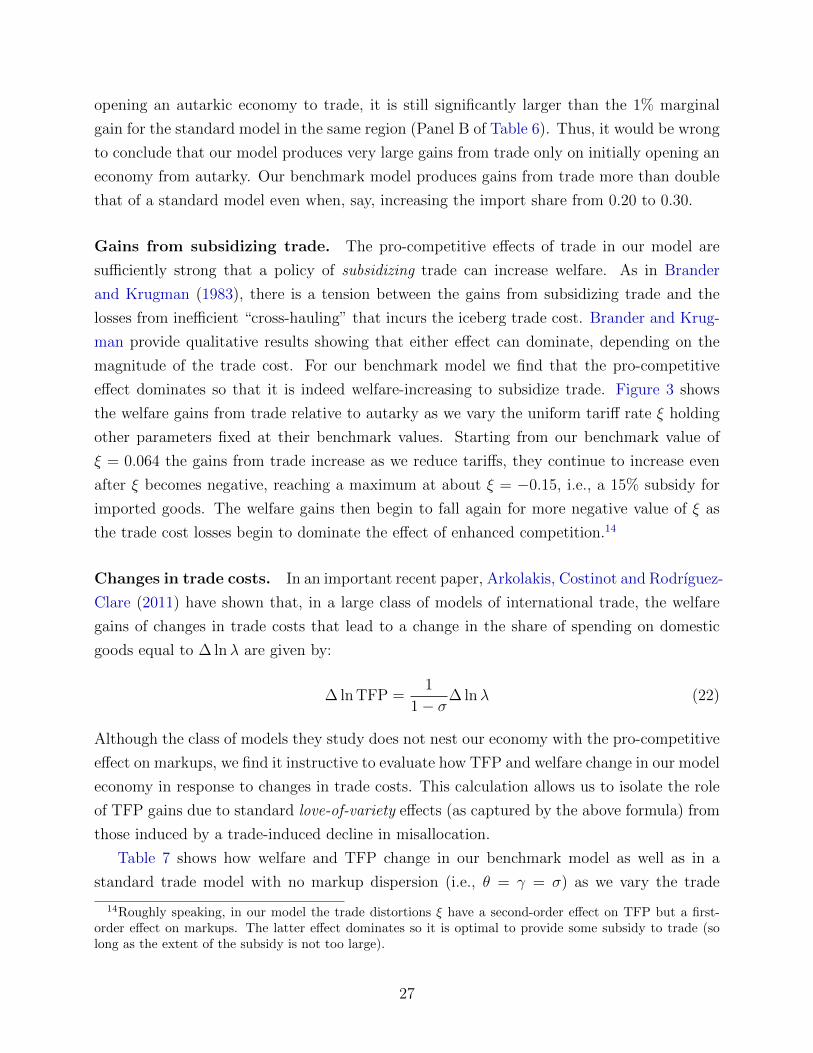
Figure 3: Gains from subsidizing trade.

Welfare gains relative to autarky for various tariff rates ξ holding other parameters fixed at theirbenchmark values. The welfare gains are maximized with about a 15% subsidy for imported goods.

26

opening an autarkic economy to trade, it is still significantly larger than the 1% marginal

gain for the standard model in the same region (Panel B of Table 6). Thus, it would be wrong

to conclude that our model produces very large gains from trade only on initially opening an

economy from autarky. Our benchmark model produces gains from trade more than double

that of a standard model even when, say, increasing the import share from 0.20 to 0.30.

Gains from subsidizing trade. The pro-competitive effects of trade in our model are

sufficiently strong that a policy of subsidizing trade can increase welfare. As in Brander

and Krugman (1983), there is a tension between the gains from subsidizing trade and the

losses from inefficient “cross-hauling” that incurs the iceberg trade cost. Brander and Krug-

man provide qualitative results showing that either effect can dominate, depending on the

magnitude of the trade cost. For our benchmark model we find that the pro-competitive

effect dominates so that it is indeed welfare-increasing to subsidize trade. Figure 3 shows

the welfare gains from trade relative to autarky as we vary the uniform tariff rate ξ holding

other parameters fixed at their benchmark values. Starting from our benchmark value of

ξ = 0.064 the gains from trade increase as we reduce tariffs, they continue to increase even

after ξ becomes negative, reaching a maximum at about ξ = −0.15, i.e., a 15% subsidy for

imported goods. The welfare gains then begin to fall again for more negative value of ξ as

the trade cost losses begin to dominate the effect of enhanced competition.14

Changes in trade costs. In an important recent paper, Arkolakis, Costinot and Rodrıguez-

Clare (2011) have shown that, in a large class of models of international trade, the welfare

gains of changes in trade costs that lead to a change in the share of spending on domestic

goods equal to ∆ lnλ are given by:

∆ ln TFP =1

1− σ∆ lnλ (22)

Although the class of models they study does not nest our economy with the pro-competitive

effect on markups, we find it instructive to evaluate how TFP and welfare change in our model

economy in response to changes in trade costs. This calculation allows us to isolate the role

of TFP gains due to standard love-of-variety effects (as captured by the above formula) from

those induced by a trade-induced decline in misallocation.

Table 7 shows how welfare and TFP change in our benchmark model as well as in a

standard trade model with no markup dispersion (i.e., θ = γ = σ) as we vary the trade

14Roughly speaking, in our model the trade distortions ξ have a second-order effect on TFP but a first-order effect on markups. The latter effect dominates so it is optimal to provide some subsidy to trade (solong as the extent of the subsidy is not too large).

27

cost to achieve different import shares. Since Arkolakis et al. (2011) abstract from capital

accumulation and assume inelastic labor supply, their welfare calculations apply to the level

of TFP. We therefore also report how TFP varies with changes in trade costs in the class of

standard trade models they consider.

Once again our model predicts substantial gains from trade. Raising the import share

from zero (τ = ∞) to 0.10 raises welfare by 24% in our model, compared to about 2.7% in

the standard trade model. Such a change in import shares raises TFP by about 13% in our

model and by about 2% in the standard trade model. Note that a 2% gain for this reduction

in trade costs is slightly larger than the gain from the Arkolakis et al. formula, equation

(22), which gives a gain of 1.48%. This slight difference arises because, in addition to trade

costs, the standard model we use also has tariffs which give rise to distortions (i.e., markups)

that depend on how much is traded. This is also why in Figure 2 the aggregate markup is

initially increasing in import shares for the standard model.

6 Robustness

We now consider several variations on our model, each designed to examine the sensitivity

of our results to parameter choices or other assumptions.

6.1 5-digit industries

Are our results driven by the focus on 7-digit industries? To examine this, we keep the

key parameters θ and γ unchanged at their benchmark values θ = 1.25 and γ = 8.5 and

recalibrate all other parameters to 5-digit data. These parameters and the moments they are

used to match are reported in Table 8. Of course at this higher level of aggregation there is

less concentration in market shares than there is at the 7-digit level, but the concentration

in the tails of the distribution is still pronounced, the 99th percentile of the distribution still

has a market share of 17%.

Table 9 reports our key results for 5-digit industries. We find that increasing the level of

aggregation to 5-digits makes almost no difference for the model’s predictions. Going from

autarky to an import share of 0.10 gives a gain of 27% in the benchmark 7-digit economy

and a slightly higher gain of 28% in the 5-digit economy. In either case, the gains from trade

are much larger than the 4% in a standard trade mode.

28

6.2 Small gap between γ and θ

If the gap between the within-industry elasticity of substitution γ and the between industry

elasticity θ is reduced, then any trade-induced variation in market shares has a smaller effect

on markups and the gains from trade in our model will tend to be smaller. Table 10 bears

this out, showing that if we increase θ from its benchmark value of 1.25 to 3, then a tariff

reduction that raises the import share from zero to 0.10 raises welfare by 8% rather than

the 27% in our benchmark. Moreover, while the level of the gains from trade is reduced, the

relative size of the gains compared to a standard trade model also fall. For an increase in the

import share from 0.10 to 0.20 or from 0.20 to 0.30, the gains in our model are larger than in

a standard model but only barely. Thus, in this setting, more of the difference in the gains

from trade comes from the effect of initially opening an economy from autarky.

Given that our quantitative results are somewhat sensitive to θ, it is worth considering

how plausible θ = 3 is for our data. A value of θ = 3 is twice as large as any of the values we

estimated (see Table 3), let alone the value of θ = 1.01 used in Atkeson and Burstein (2008).

It is close to the θ = 3.79 used in Bernard et al. (2003), but they effectively have γ =∞ and

so retain a large gap between the within- and between-industry elasticities rather than the

narrower gap that is being considered in this experiment.

6.3 Bertrand competition

In our benchmark model we assume that firms compete in Cournot fashion, i.e., choosing

quantities. If we instead assume that firms compete in Bertrand competition, choosing

prices, then the model changes in only one respect. The demand elasticity facing producer i

in industry j is no longer a weighted harmonic average of θ and γ, as in equation (9), but is

now just a simple average:

εij = ωijθ + (1− ωij) γ. (23)

Qualitatively, the intuition for this demand elasticity is the same as in the Cournot case. If

a producer is a near-monopolist in its own industry, then the relevant competition is from

firms in other industries so the demand elasticity is the lower value θ. But if a producer has

very little market share its own industry, the elasticity is the higher value γ.

To examine the quantitative implications of Bertrand competition in our model, we keep

the elasticities θ = 1.25 and γ = 8.5 as in the benchmark but recalibrate the other model

parameters to match the same moments as before. Table 10 shows that when we do this, the

gains from trade increase slightly relative to the Cournot benchmark. In particular, going

from autarky to an import share of 0.10 gives a gain of 34% with Bertrand competition as

against 27% with Cournot. The marginal gains from trade diminish a little more rapidly

29

with Bertrand competition, going from an import share of 0.10 to 0.20 gives an additional

gain of 2.9% with Bertrand instead of the 6.2% with Cournot. However, as with the high θ

case, with Bertrand competition the relative size of the gains compared to a standard trade

model also fall. For an increase in the import share from 0.10 to 0.20 or from 0.20 to 0.30,

the gains in our model are larger than in a standard model but not by much.

Bertrand vs. Cournot. The Cournot and Bertrand specifications have broadly similar

aggregate productivity and overall welfare implications. We chose the Cournot specification

for the benchmark case because it allows us to better match the micro data on labor shares and

market shares. As in equation (12), the Cournot case implies a linear decreasing relationship

between labor shares and market shares. Bertrand competition implies a decreasing but

strictly concave relationship. If anything, the data gives a slightly convex relationship which

the linear Cournot case is better able to match.

6.4 Uncorrelated productivity

In our benchmark model, firm-level productivity draws at home aij and abroad a∗ij are per-

fectly correlated. Thus, if under autarky a given industry contains a large, dominant firm

that charges a high markup and produces relatively too little, opening up to trade confronts

that firm with a similarly productive firm that can compete effectively (though hampered

by trade costs and any remaining tariff barriers). If, however, that large domestic firm was

not systematically likely to face competition from a similarly productive firm, then the pro-

competitive effects of trade will be diminished. To assess the quantitative significance of our

assumption that productivity is perfectly correlated, we solve our model assuming aij and a∗ij

are uncorrelated draws from (20). We choose uncorrelated draws rather than some degree of

partial correlation so as to make the comparison as stark as possible.

Similar overall gains from trade. For this exercise, we again keep θ = 1.25 and γ = 8.5

but recalibrate the other model parameters to match the same moments as before. The

results are shown in Table 10. With uncorrelated productivity, moving from autarky to a

0.10 import share leads to a gain of 14% as opposed to 27% in the benchmark model with

correlated productivity. This is still considerably larger than in the standard trade model

where the gain is about 9% when productivity is uncorrelated. However, with uncorrelated

productivity, the diminishing marginal gains from trade does not set in so quickly. Indeed,

going from a 0.10 to 0.20 import share gives an additional gain of 19% as opposed to an

additional gain of 6% in the benchmark. Adding these up, going from autarky to a 0.20

30

import share gives a gain of 33.5% in the benchmark model with correlated productivity and

an almost identical 33.3% with uncorrelated productivity.

Different composition of gains from trade. Why are the overall gains from trade so

similar despite the lack of correlation? The short answer is that the composition of the

gains from trade changes greatly; with uncorrelated productivity the aggregate markup is

essentially unchanged, but the gains from the standard love-of-variety channel are now much

larger. The love-of-variety effect is larger because, endogenously, the Armington elasticity

falls substantially as the economy becomes open to trade. The uncorrelated productivity

translates to greater industry-level dispersion in import shares, which, via equation (19),

reduces the Armington elasticity. In this exercise, increasing the import share from autarky

to 0.20 reduces the Armington elasticity from 8.5 to 2.8. This implies larger misallocation

losses in autarky and hence larger gains from trade. Indeed, even a standard trade model

would produce fairly substantial gains from trade if given an Armington elasticity as low as

2.8. This increase in the gains from love-of-variety completely offsets the decreased gains

from the pro-competitive effect.

Why correlated productivity matters. In essence, having perfectly correlated produc-

tivity is akin to assuming that more trade brings more competition (though the significance

of that extra competition is a quantitative question). We view the assumption of correlated

productivity draws as being reasonable for a small economy like Taiwan; it is presumably

less reasonable for a country like the U.S. with a large domestic market and many producers

that will not face more productive rivals even if trade barriers are lowered.

However, since all heterogeneity in goods in this model is captured by productivity dif-

ferences (e.g., there are no product- or industry-level differences in consumer expenditure

shares), even for large countries like the U.S. it would be perhaps more realistic to have some

partial correlation across products to capture these attributes.

Again, micro details matter. This exercise highlights that, when calculating the welfare

gains from trade in our model, it is important to properly account for the micro details

even when the competitive effects of trade turn out to be weak. Although the model with

uncorrelated productivity results in lower gains from the pro-competitive effect, in order

to correctly calculate these gains it is essential to determine how the Armington elasticity

changes with policy. Micro details such as as the dispersion of industry-level import shares

are endogenous to policy and determine the magnitude of the the induced changes in the

Armington elasticity and therefore the size of the gains from the standard love-of-variety

31

effect (this is true with a common tariff ξ, it is likely to be only more true if we had good-

specific trade barriers). Put differently, in this model correctly calculating the gains from

trade requires knowing the magnitude of the Armington elasticity after the policy change,

but that magnitude cannot be determined independently of the micro details. By contrast, in

the large class of trade models covered by the Arkolakis et al. (2011) formula, the Armington

elasticity is constant and these micro details are irrelevant for welfare.

7 Evidence for the pro-competitive mechanism

Our model predicts that industries with higher import shares are characterized by more

competition, and therefore both lower revenue (labor) productivity and lower dispersion in

revenue productivity. We next describe the evidence from the Taiwanese manufacturing data

on these predictions of the model.

Revenue productivity and import shares. Panel A of Table 11 reports regressions of

log revenue productivity in industry j on log import shares in industry j for the Taiwanese

manufacturing data. Consistent with the theory, we find that industries with higher import

shares have substantially lower labor productivity. The elasticity of labor productivity with

respect to import share ranges from −0.13 (unweighted regression) to −0.26, with standard

errors in the range of 0.02 or 0.03. This is an economically substantial effect. For the

unweighted regression, for example, increasing the import share from zero (autarky) to 0.50

leads to a 6.5% drop in revenue productivity (i.e., −0.13× 0.5 = −0.065).

Controlling for variation in capital intensities αi. One concern with these regressions

is that revenue productivity variation across industries might be driven by variation in capital

intensities or other inputs rather than variation in markups. In particular, more tradable

goods may be more capital intensive. To examine this, we observe from (11) that if a firm

has capital intensity αi then its markup is:

mi =εi

εi − 1= (1− αi)

piyiwili

.

That is, if we have two firms with different capital intensities but the same labor productivity,

the firm with the higher αi will have a lower measured markup mi. For each industry we

compute the weighted average of mi and regress it on industry-level import shares. We find,

if anything, that the reduction in productivity in higher import share industries is even larger

than for just labor productivity. The elasticity of productivity with respect to import share

32

now varies from −0.21 (unweighted regression) to −0.45 (weighted regression). Thus cross-

sectional variation in capital intensity does not drive our finding that higher import share

industries have lower productivity.

Dispersion in labor productivity. Panel B of Table 11 shows that the dispersion in labor

productivity across producers within an industry is also negatively related to the industry

import share. In the model, most of the change in markup dispersion induced by changes in

trade come from changes in the tails of the distribution. Given this, in the table we report

industry-level productivity dispersion as the gap between the 95th and 50th percentiles of

the distribution. This gives elasticities varying from −0.13 (unweighted) to −0.20 with

standard errors around 0.03. We obtain similar results when controlling for variation in

capital intensities.

Pro-competitive effects in the empirical trade literature. A large literature studies

the links between markups and import competition. A key challenge in this literature is that

measuring markups is difficult because neither prices nor marginal cost are typically observ-

able at the firm/plant level. Two common methods exist for addressing this difficulty are

the use of price/cost margin (PCM) regressions15 or the generalized Solow residual approach

developed by Hall (1988). Tybout (2003) systematically reviews the evidence from both

methods for many countries. For example, when PCM regressions implemented with plant-

level panel data, the “results for Mexico (1985-90), Colombia (1977-85), Chile (1979-86), and

Morocco (1984-89) all reveal the same basic pattern: in every country studied, relatively

high industry-wide exposure to foreign competition is associated with lower price-cost mar-

gins, and the effect is concentrated in larger plants.” Grether (1996) explores alternative

measures of import competition and find these patterns robust for Mexico. Various studies

have also investigated trade liberalization episodes using Hall’s framework. Comparing pre-

and post-liberalization estimates, Levinsohn (1993), Harrison (1994), and Krishna and Mitra

(1998) find evidence that, an increase in foreign competition, over time, drives down domes-

tic firm markups in Turkey, Cote d’Ivoire, and India respectively. Several other studies have

used more highly aggregated industry-level data but with longer time series to document

the pro-competitive effects of trade. For example, recently Chen, Imbs and Scott (2009)

have estimated a version of the Melitz and Ottaviano model using EU manufacturing data

covering 1989-1999. They find short-run evidence that trade openness exerts a competitive

effect with prices and markups falling.

15PCMs are the ratio of revenue less variables costs to variable costs. Under the assumption of constantmarginal costs, this ratio is a monotonic transformation of the markup.

33

8 Conclusions

We calculate the gains from international trade in a quantitative model with endogenously

variable markups. We find that the welfare gains from trade can be large and, in particular,

can be an order of magnitude larger that those implied by standard trade models with

constant markups.

In our model, a trade-induced fall in markups increases welfare through two distinct

channels: by reducing average markups, and by reducing dispersion in markups. The first

effect directly reduces distortions in labor and investment decisions. The second effect reduces

relative producer price distortions, thereby promoting a more efficient allocation of resources

across firms and increasing aggregate TFP. We quantify the model using product-level data

for Taiwanese manufacturing establishments and find that both effects can be substantial.

This pro-competitive mechanism implies that industries with high exposure to international

competition have substantially lower average revenue productivity and lower dispersion in

revenue productivity than in industries that face little such competition. We find direct

evidence in support of these predictions in the Taiwanese micro data.

The main message of our paper, however, is not that the gains from trade are “always and

everywhere” large. Rather, our conclusion is that to quantify the welfare gains from trade

requires getting the micro details right. In our benchmark model, the gains from trade are

large and operate through a pro-competitive mechanism that is not emphasized in standard

models with constant markups. And while we find smaller effects from the pro-competitive

mechanism in some of our robustness experiments, even then we find that the micro details

matter. Irrespective of the size of the pro-competitive effects, to correctly calculate the gains

from trade in our model requires correctly determining how the Armington elasticity changes

with the change in trade policy. Micro details such as as the dispersion of industry-level

import shares determine the change in the Armington elasticity and therefore also determine

the size of the gains from standard love-of-variety effects, not just pro-competitive effects.

To keep our paper focussed we have made a number of important simplifying assump-

tions. For example, we have focussed exclusively on intraindustry trade and, in the tradition

of such models, have abstracted from aggregate differences in technologies or factor endow-

ments. It would be interesting to understand the between-country relative gains from the

pro-competitive effects trade when two countries of different sizes and/or different aggregate

technologies become more integrated. Similarly, in our experiments we have always consid-

ered symmetric changes in trade policy. It would be interesting to consider the gains from

trade in our model from unilateral changes in trade policy. Finally, by adopting a repre-

sentative consumer framework, we have abstracted from all issues of the distribution of the

34

within-country gains from trade. We consider all these issues to be important directions for

future research.

35

Tab

le1:

Dat

aD

escr

ipti

on

Pan

elA

:A

nex

ampl

eof

prod

uct

clas

sifi

cati

on

3-dig

it31

4-

com

pute

rsan

dst

orag

eeq

uip

men

t

5-dig

it31

410

-co

mpute

rs

7-dig

it31

4100

0-

min

i-co

mpute

r31

4101

0-

wor

k-s

tati

on31

4102

1-

des

kto

pco

mpute

r31

4102

2-

lapto

pco

mpute

r31

4102

3-

not

ebook

com

pute

r31

4102

4-

pal

mto

pco

mpute

r31

4102

5-

pen

-bas

edco

mpute

r31

4102

6-

han

dhel

dco

mpute

r31

4102

7-

elec

tron

icdic

tion

ary

Pan

elB

:D

istr

ibu

tion

ofpr

odu

cts

and

indu

stri

es

2-dig

it4-

dig

it7-

dig

it(s

ecto

r)(i

ndust

ry)

(pro

duct

s)

texti

le16

76ap

par

el10

39le

ather

433

lum

ber

615

furn

iture

412

pap

er6

23pri

nti

ng

34

chem

ical

mat

eria

ls7

152

chem

ical

pro

duct

s9

83p

etro

leum

212

rubb

er3

16pla

stic

s7

34cl

ay/g

lass

/sto

ne

1847

pri

mar

ym

etal

1499

fabri

cate

dm

etal

1465

indust

rial

mac

hin

ery

2916

3co

mpute

r/el

ectr

onic

s11

136

elec

tron

icpar

ts6

72el

ectr

ical

mac

hin

ery

1112

5tr

ansp

orta

tion

1299

inst

rum

ents

770

36

Tab

le2:

Par

amet

eriz

atio

n

Pan

elA

:M

omen

ts Dat

aM

odel

Con

cen

trat

ion

stat

isti

csex

cl.

impo

rter

s

mea

nin

vH

H7.

255.

41m

edia

nin

vH

H3.

954.

42m

ean

hig

hes

tsh

are

0.45

0.50

med

ian

hig

hes

tsh

are

0.39

0.39

Con

cen

trat

ion

stat

isti

csin

cl.

impo

rter

s

mea

nsh

are

0.02

90.

029

s.d.

shar

e0.

087

0.07

7m

edia

nsh

are

0.00

360.

0049

75th

p.c

.sh

are

0.01

60.

016

95th

p.c

shar

e0.

141

0.14

199

thp.c

.sh

are

0.46

10.

474

Add

itio

nal

stat

isti

cs

mea

nin

dust

ryim

por

tsh

are

0.26

0.26

frac

tion

exp

ort

0.25

0.25

Arm

ingt

onel

asti

city

88

Pan

elB

:P

aram

eter

s

Cal

ibra

ted

N,

num

ber

com

pet

itor

s80

µ,

Par

eto

dis

trib

uti

onsh

ape

4.2

H,

upp

erb

ound

80p H

,m

ass

atupp

erb

ound

0.00

35Ff,

fixed

cost

exp

ort,

%S.S

.la

bor

3.6

Fd,

fixed

cost

,%

S.S

.la

bor

2.3

γ,

elas

tici

tyw

ithin

indust

ry8.

50τ,

iceb

erg

trad

eco

st0.

22

Ass

ign

ed

θ,el

asti

city

bet

wee

nin

dust

ries

1.25

β,

dis

count

fact

or0.

96δ,

capit

aldep

reci

atio

n0.

10α

,ca

pit

alin

tensi

ty0.

33ξ,

tari

ffra

te0.

064

37

Table 3: Estimates of θ

Panel A: Exclude exporters

Drop if share > 0.9 All observations

OLS 1.23 1.38(0.039) (0.046)

median regression 1.20 1.35(0.046) (0.053)

# observations 58895 58920

Panel B: Include exporters

Drop if share > 0.9 All observations

OLS 1.20 1.33(0.036) (0.041)

median regression 1.18 1.30(0.039) (0.045)

# observations 64677 64705

Panel C: Labor and capital shares

Drop if share > 0.9 All observations

OLS 1.13 1.28(0.032) (0.033)

median regression 1.04 1.13(0.033) (0.032)

# observations 26498 26509

(Assumed 15% user cost in Panel C)

38

Table 4: Additional Micro Implications

Data Model

mean markup 1.17s.d. markup 0.11

median markup 1.1475th p.c. markup 1.1595th p.c. markup 1.2799th p.c. markup 1.79

s.d. labor product. 0.68 0.10

mean labor share 0.61 0.62median labor share 0.65 0.62

aggregate labor share 0.43 0.45

39

Table 5: Losses Due to Markups

Panel A: Benchmark model

Benchmark First-Best No markup dispersion

markup 1.47 1 1.47∆ ln TFP − 0.05 0.05

∆ lnY − 0.57 0.07∆ lnC − 0.48 0.07∆ lnL − 0.31 0

welfare gains, % − 16.7 6.5

Panel B: Autarky

Benchmark First-Best No markup dispersion

markup 1.69 1 1.69∆ ln TFP − 0.23 0.23

∆ lnY − 1.01 0.35∆ lnC − 0.89 0.35∆ lnL − 0.41 0

welfare gains, % − 48.9 31.6

40

Table 6: Gains from Trade due to Reductions in Tariffs

Panel A: Benchmark model

∆ import share 0 to 10% 10 to 20% 20 to 30%

welfare gains, % 27.3 6.2 3.0

∆ ln markup −0.08 −0.04 −0.04∆ ln TFP 0.17 0.03 0.01

∆ lnY 0.35 0.10 0.07∆ lnC 0.34 0.09 0.06∆ lnL 0.06 0.03 0.03

Armington elasticity 8.5 to 7.5 7.5 to 7.9 7.9 to 8.2

Panel B: Standard trade model

∆ import share 0 to 10% 10 to 20% 20 to 30%

welfare gains, % 4.3 2.3 1.3

∆ ln markup 0.02 0.00 −0.01∆ ln TFP 0.04 0.02 0.01

∆ lnY 0.03 0.02 0.03∆ lnC 0.03 0.02 0.02∆ lnL −0.02 0.00 0.01

Armington elasticity 8.1 8.1 8.1

41

Table 7: Gains from Trade due to Reductions in Trade Costs

Panel A: Benchmark model

∆ import share 0 to 10% 10 to 20% 20 to 30%

welfare gains, % 23.7 8.0 6.4

∆ ln markup −0.12 −0.02 −0.01∆ ln TFP 0.13 0.05 0.04

∆ lnY 0.34 0.10 0.07∆ lnC 0.32 0.10 0.07∆ lnL 0.09 0.02 0.00

Armington elasticity 8.5 to 7.5 7.5 to 7.9 7.9 to 8.2

Panel B: Standard trade model

∆ import share 0 to 10% 10 to 20% 20 to 30%

welfare gains, % 2.7 2.9 3.2

∆ ln markup 0.01 0.01 0.01∆ ln TFP 0.02 0.02 0.03

∆ lnY 0.02 0.03 0.03∆ lnC 0.03 0.03 0.03∆ lnL −0.01 −0.01 −0.01

Armington elasticity 8 8 8

42

Tab

le8:

Par

amet

eriz

atio

nof

Eco

nom

yC

alib

rate

dto

5-D

igit

Indust

ries

Pan

elA

:M

omen

ts Dat

aM

odel

Con

cen

trat

ion

stat

isti

csex

cl.

impo

rter

s

mea

nin

vH

H14

.90

12.2

3m

edia

nin

vH

H7.

9710

.40

mea

nhig

hes

tsh

are

0.30

0.41

med

ian

hig

hes

tsh

are

0.25

0.24

Con

cen

trat

ion

stat

isti

csin

cl.

impo

rter

s

mea

nsh

are

0.01

10.

010

s.d.

shar

e0.

040

0.04

0m

edia

nsh

are

0.00

140.

0026

75th

p.c

.sh

are

0.00

60.

006

95th

p.c

shar

e0.

044

0.03

399

thp.c

.sh

are

0.17

30.

156

Add

itio

nal

stat

isti

cs

mea

nin

dust

ryim

por

tsh

are

0.26

0.26

frac

tion

exp

ort

0.25

0.25

Arm

ingt

onel

asti

city

88

Pan

elB

:P

aram

eter

s

Cal

ibra

ted

N,

num

ber

com

pet

itor

s10

0µ

,P

aret

odis

trib

uti

onsh

ape

6.56

H,

upp

erb

ound

31p H

,m

ass

atupp

erb

ound

0.00

35Ff,

fixed

cost

exp

ort,

%S.S

.la

bor

2.4

Fd,

fixed

cost

,%

S.S

.la

bor

0.5

γ,

elas

tici

tyw

ithin

indust

ry8.

50τ,

iceb

erg

trad

eco

st0.

15

Ass

ign

ed

θ,el

asti

city

bet

wee

nin

dust

ries

1.25

β,

dis

count

fact

or0.

96δ,

capit

aldep

reci

atio

n0.

10α

,ca

pit

alin

tensi

ty0.

33ξ,

tari

ffra

te0.

064

43

Table 9: Gains from Trade due to Reductions in Tariffs

Economies calibrated to 7- and 5-digit industries

Standard 7-digit 5-digit

0 to 10% 4.3 27.3 27.8

10 to 20% 2.3 6.2 5.9

20 to 30% 1.3 3.0 2.8

Table 10: Gains from Trade due to Reductions in Tariffs

Additional robustness experiments

Benchmark Armington = 5 θ = 3 Bertrand Uncorrelated

0 to 10% 27.3 22.6 8.2 34.0 14.2(4.3) (6.6) (4.3) (4.3) (8.8)

10 to 20% 6.2 7.6 2.7 2.9 19.1(2.3) (3.7) (2.3) (2.3) (8.5)

20 to 30% 3.0 4.3 1.4 1.4 15.8(1.3) (2.0) (1.3) (1.3) (5.3)

Armington 8 5 8 8 8.5, 3.8, 2.8, 4.2

Note: This table reports the consumption-equivalent change in welfare (including transitions) We report (inbrackets) the welfare gains of the corresponding standard model (i.e., the model with the same Armingtonelasticity) For all models, except the Uncorrelated Shocks, we report the Armington elasticity for Taiwan’simport share For the model with Uncorrelated Shocks, we report the Armington elasticity at 0%, 10%, 20%and 30% import shares For the model with Uncorrelated Shocks, we report the welfare gains of the standardmodel with an Armington elasticity of 3.8, 2.8 and 2.8, respectively, i.e., the lowest elasticity in that rangeof trade shares in the model with endogenous markups

44

Table 11: Trade and Productivity in Taiwanese Manufacturing

Panel A: Industry productivity vs. industry import share

Unweighted Weighted

labor productivity −0.125 −0.260(0.023) (0.029)

(labor + capital) productivity −0.214 −0.452(0.046) (0.047)

Panel B: Industry productivity dispersion vs. import share

Unweighted Weighted

labor productivity −0.130 −0.198(0.032) (0.036)

(labor + capital) productivity −0.127 −0.285(0.029) (0.040)

Statistics are computed for non-exporting plants We measure dispersion in productivity as the 95th minus50th percentile

45

References

Anderson, James E. and Eric van Wincoop, “Trade Costs,” Journal of EconomicLiterature, September 2004, 42 (3), 691–751.

Arkolakis, Costas, Arnaud Costinot, and Andres Rodrıguez-Clare, “Gains FromTrade under Monopolistic Competition: A Simple Example with Translog ExpenditureFunctions and Pareto Distributions of Firm-Level Productivity.,” 2010. Yale Unviersityworking paper.

, , and , “New Trade Models, Same Old Gains?,” American Economic Review, 2011,forthcoming.

Armington, Paul S., “A Theory of Demand for Products Distinguished by Place of Pro-duction,” IMF Staff Papers, March 1969, 16 (1), 159–178.

Atkeson, Andrew and Ariel Burstein, “Pricing-to-Market, Trade Costs, and Interna-tional Relative Prices,” American Economic Review, 2008, 98 (5), 1998–2031.

Aw, Bee Yan, Sukkyun Chung, and Mark J. Roberts, “Productivity and Turnoverin the Export Market: Micro-Level Evidence from the Republic of Korea and Taiwan,”World Bank Economic Review, January 2000, 14 (1), 65–90.

Bernard, Andrew B., Jonathan Eaton, J. Bradford Jensen, and Samuel Kortum,“Plants and Productivity in International Trade,” American Economic Review, September2003, 93 (4), 1268–1290.

, Stephen J. Redding, and Peter Schott, “Multiple-Product Firms and ProductSwitching,” American Economic Review, March 2010, 100 (1), 70–97.

Bottasso, Anna and Alessandro Sembenelli, “Market Power, Productivity, and the EUSingle Market Program: Evidence from a Panel of Italian Firms,” European EconomicReview, January 2001, 45 (1), 167–186.

Brander, James A., “Intra-Industry Trade in Identical Commodities,” Journal of Inter-national Economics, February 1981, 11 (1), 1–14.

and Paul R. Krugman, “A ‘Reciprocal Dumping’ Model of International Trade,” Jour-nal of International Economics, November 1983, 15 (3-4), 313–321.

Broda, Christian and David E. Weinstein, “Globalization and the Gains from Variety,”Quarterly Journal of Economics, May 2006, 121 (2), 541–585.

Campbell, Jeffrey R. and Hugo A. Hopenhayn, “Market Size Matters,” Journal ofIndustrial Economics, 2005, 53 (1), 1–25.

Chen, Natalie, Jean Imbs, and Andrew Scott, “The Dynamics of Trade and Compe-tition,” Journal of International Economics, February 2009, 77 (1), 50–62.

46

De Blas, Beatriz and Katheryn Russ, “Teams of Rivals: Endogenous Markups in aRicardian World,” 2010. NBER Working Paper 16587.

Devereux, Michael B. and Khang Min Lee, “Dynamic Gains from International Tradewith Imperfect Competition and Market Power,” Review of Development Economics, 2001,5 (2), 239–255.

Dixit, Avinash K. and Joseph E. Stiglitz, “Monopolistic Competition and OptimumProduct Diversity,” American Economic Review, 1977, 67 (3), 297–308.

Eaton, Jonathan and Samuel Kortum, “Technology, Geography, and Trade,” Econo-metrica, September 2002, 70 (5), 1741–1779.

Epifani, Paolo and Gino Gancia, “Trade, Markup Heterogeneity, and Misallocations,”Journal of International Economics, January 2011, 83 (1), 1–13.

Feenstra, Robert C. and David E. Weinstein, “Globalization, Markups, and the U.S.Price Level,” 2010. NBER Working Paper 15749.

, Maurice Obstfeld, and Katheryn Russ, “In Search of the Armington Elasticity,”2010. UC Davis working paper.

Grether, Jean-Marie, “Mexico, 1985-90: Trade Liberalization, Market Structure and Man-ufacturing Performance,” in Mark J. Roberts and James R. Tybout, eds., Industrial Evo-lution in Developing Countries, Oxford University Press. New York. 1996.

Hall, Robert E., “The Relation Between Price and Marginal Cost in U.S. Industry,” Journalof Political Economy, October 1988, 96 (5), 921–947.

Harrison, Ann E., “Productivity, Imperfect Competition and Trade Reform: Theory andEvidence,” Journal of International Economics, February 1994, 36 (1), 53–73.

Holmes, Thomas J. and James A. Schmitz, “Competition and Productivity: A Reviewof the Evidence,” Annual Review of Economics, September 2010, 2, 619–642.

, Wen-Tai Hsu, and Sanghoon Lee, “Plants, Productivity and Market-Size with Head-to-Head Competition,” 2011. FRB Minneapolis working paper.

Hsieh, Chang-Tai and Peter J. Klenow, “Misallocation and Manufacturing TFP inChina and India,” Quarterly Journal of Economics, November 2009, 124 (4), 1403–1448.

Imbs, Jean and Isabelle Mejean, “Elasticity Optimism,” May 2011. Paris School ofEconomics working paper.

Krishna, Pravin and Devashish Mitra, “Trade Liberalization, Market Discipline, andProductivity Growth: New Evidence from India,” Journal of Development Economics,August 1998, 56 (2), 447–462.

47

Krugman, Paul R., “Increasing Returns, Monopolistic Competition, and InternationalTrade,” Journal of International Economics, November 1979, 9 (4), 469–479.

, “Scale Economics, Product Differentiation, and the Pattern of Trade,” American Eco-nomic Review, December 1980, 70 (5), 950–959.

Levinsohn, James A., “Testing the Imports-as-Market-Discipline Hypothesis,” Journal ofInternational Economics, August 1993, 35 (1), 1–22.

Melitz, Marc J., “The Impact of Trade on Intra-Industry Reallocations and AggregateIndustry Productivity,” Econometrica, November 2003, 71 (6), 1695–1725.

and Giancarlo I.P. Ottaviano, “Market Size, Trade, and Productivity,” Review ofEconomic Studies, 2008, 75 (1), 295–316.

Novy, Dennis, “International Trade without CES: Estimating Translog Gravity,” 2010.Discussion Paper 1031, Centre for Economic Performance, London School of Economics.

Pavcnik, Nina, “Trade Liberalization, Exit and Productivity Improvement: Evidence fromChilean Plants,” Review of Economic Studies, January 2002, 69 (1), 245–276.

Peters, Michael, “Heterogeneous Markups and Endogenous Misallocation,” 2011. MITworking paper.

Restuccia, Diego and Richard Rogerson, “Policy Distortions and Aggregate Produc-tivity with Heterogeneous Establishments,” Review of Economic Dynamics, October 2008,11 (4), 707–720.

Rogerson, Richard and Johanna Wallenius, “Micro and Macro Elasticities in a Life-Cycle Model with Taxes,” Journal of Economic Theory, November 2009, 144, 2277–2292.

Tybout, James R., “Plant- and Firm-Level Evidence on “New” Trade Theories,” inE. Kwan Choi and James Harrigan, eds., Handbook of International Trade, Basil Blackwell.Oxford. 2003.

48