Embed Size (px)
Citation preview
Competition in Electricity Markets withRenewable Energy Sources∗
Daron Acemoglu† Ali Kakhbod‡ Asuman Ozdaglar§
First draft: June 2014
This draft: May 2015
Abstract
This paper studies the effects of the diversification of energy portfolios on the merit
order effect in an oligopolistic energy market. The merit order effect describes the neg-
ative impact of renewable energy, typically supplied at the low marginal cost, to the
electricity market. We show when thermal generators have a diverse energy portfo-
lio, meaning that they also control some or all of the renewable supplies, they offset
the price declines due to the merit order effect because they strategically reduce their
conventional energy supplies when renewable supply is high. In particular, when all
renewable supply generates profits for only thermal power generators this offset is
complete — meaning that the merit order effect is totally neutralized. As a conse-
quence, diversified energy portfolios may be welfare reducing. These results are ro-
bust to the presence of forward contracts and incomplete information (with or without
correlated types). We further use our full model with incomplete information to study
the volatility of energy prices in the presence of intermittent and uncertain renewable
supplies.
Keywords: Merit order effect, imperfect competition, geographic proximity, di-
versification, oligopoly pricing, intermittent sources
JEL Classification: D6, D62.
∗We thank seminar participants at MIT, UC Berkeley and the 2014 Allerton Conference for helpful com-ments.
†Department of Economics, Massachusetts Institute of Technology (MIT), Cambridge, MA, 02139, USA.Email: [email protected]
‡Department of Economics, Massachusetts Institute of Technology (MIT), Cambridge, MA 02139, USA.Email: [email protected].
§Laboratory for Information and Decision Systems (LIDS), Massachusetts Institute of Technology (MIT),Cambridge, MA 02139, USA. Email: [email protected].

1 Introduction
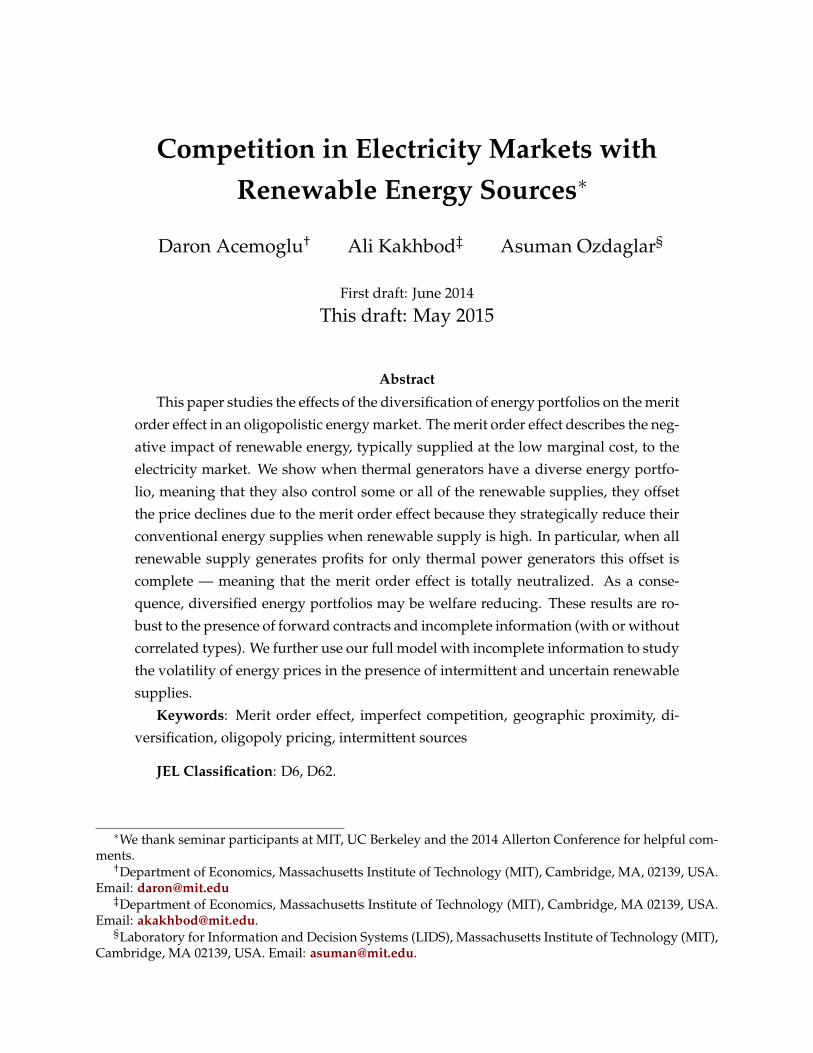
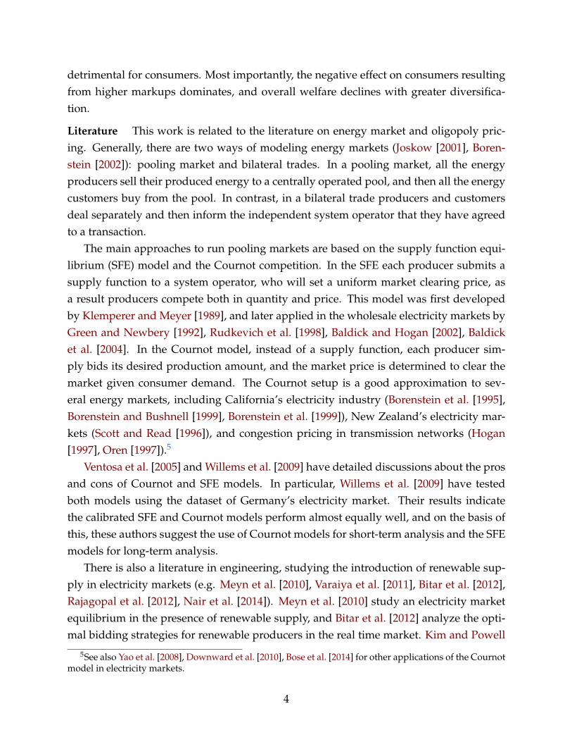
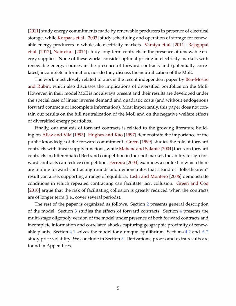
With mounting concerns over climate change caused by fossil fuels, there has been grow-ing reliance on renewable energy.1 Currently, 67 countries, including all EU countries,have renewable energy policy targets, mandating electricity companies to provide a min-imal fraction of total electricity supply from renewables. In the United States, for example,this target is set to grow to 20% by 2020, while it is 33% in the UK and also 20% in the Eu-ropean Union. These targets have motivated many conventional (thermal) energy com-panies to seek a diversified energy portfolio and increase their investments in renewablesupply. The European energy giant Alstom has thus concluded: “A diverse energy port-folio is the only sound business and policy strategy able to address any Energy & Climatescenario” (Lalwani and Khoo [2013]). Though the high setup costs of renewable plantsare often subsidized by public funds (U.S. Energy Information Administration [2013]),they are argued to benefit the economy not just by reducing fossil fuel emissions but alsoby delivering cheaper energy to consumers through the merit order effect (MoE). The meritorder effect arises because renewable energy has negligible marginal costs and reducesthe spot equilibrium price as illustrated in Figure 1.2 Figure 2 depicts the merit ordereffect in action in the German market and shows the strong negative correlation betweenthe supply of (intermittent) renewable energy and the wholesale electricity price.3
This paper argues that the objective of a diversified energy portfolio of conventionalenergy companies conflicts with the presumed benefits from increasing supply of renew-ables in terms of lower prices (via the merit order effect). We show that when the increasein the supply of renewable energy takes the form of diversified energy portfolios, theMoE is partially neutralized. In the extreme case where all of the supply of renewablescomes in the form of such diversified energy portfolios (meaning that it is supplied bythe same conventional energy companies), the MoE is fully neutralized, and greater re-newable supplies, or more favorable realization of renewable supply outcomes, have noimpact on equilibrium energy prices.
Our baseline and simplest model uses the standard Cournot oligopolistic competitionsetup to establish the partial or full neutralization of the MoE. The main economic forceleading to this result is that diversified producers have an incentive to offset the price de-clines due to the MoE by reducing their conventional energy supplies. The greater is the
1For the climate and environmental benefits of renewable energy, see for example Dincer [2000].2In addition, renewable energy also enjoys priority dispatch due to regulation.3The merit order effect is also documented in detail in several other seen in several electricity markets
(e.g. German market (Sensfuss et al. [2008], Nicolosi and Fursch [2009], Cludiusa et al. [2014]), German-Austrian market (Wurzburg et al. [2013]), Danish market (Munksgaarda and Morthorstb [2008]), Irish mar-ket (O’Mahoney and Eleanor [2011]), and Australian market (McConnella et al. [2013])).
1
Renewable Supply
Demand
Supply with RES
Supply without RES
Price
Quantity
Price
Decrease
Figure 1: The merit order effect on the equilibrium (market) prices.
Figure 2: The relationship between prices in red ($/MWh) and renewable energy outputin blue (MWh) in Germany. Source: European Energy Exchange (EEX).
2
supply of renewables, the stronger is this incentive. This force is related to the strategicsubstitutes property of Cournot competition, inducing suppliers to cut production whenthe supply of renewables is high. But crucially, this incentive is exacerbated because di-versified energy companies take into account the loss of profits from their own renewablesupplies that would result in the absence of such a cut.
We then enrich this baseline model to incorporate two important features of energymarkets: forward contracts, and correlated imperfectly observed shocks to geographi-cally proximate renewable energy suppliers. Forward contracts play a central role inmany energy markets, both because of private parties’ incentives to hedge pricing riskand because of regulations mandating forward contracts for generators.4 We analyze for-ward contracts by adapting the seminal work of Allaz and Vila [1993], who demonstratedthat forward contracts lead to lower equilibrium prices in oligopolistic markets. We showthat our main results on the partial and full neutralization of the MoE applies in the pres-ence of forward contracts in exactly the same fashion as in our baseline model.
Our full model incorporates both forward contracts and correlated, imperfectly ob-served shocks. We model this latter feature by assuming that renewable energy suppliesin similar geographic areas are subject to locally correlated variability, and that each firmonly observes its own realization of renewable supply, but is aware of the structure of lo-cal correlation. We are not aware of any other work in the literature developing a tractablemodel of incomplete information Cournot equilibrium with forward contracts and renew-able energy. The incomplete information Cournot equilibrium in this case again showsthe neutralization of the MoE. In addition, this version of the model enables us to studythe implications of renewable supply on price volatility. Focusing on spatial configura-tions in which the correlation of renewable supply decays according to distance acrossplants, we show that the spot price volatility increases as the distance among renewableplants increases. This is because when renewable plants are far apart so that there is lesscorrelation among renewable supply, they create more miscoordination in supplies, in-creasing price volatility. Using this intuition, we further show that among all geographicconfigurations with “regular” structures, the maximum price volatility occurs when re-newable plants have a “ring” structure and the minimum price volatility arises in geo-graphic configurations exhibiting a “complete” structure.
Finally, we study the profit and welfare implications of diversified renewable port-folios. Intuitively, diversified energy portfolios are beneficial for thermal producers, but
4This is because of concerns that without forward contracts, the generators (with market power) maymanipulate energy prices (e.g., Borenstein [2002]). Empirical research also indicates the extent of forwardcontracting by generators has been an important determinant of the competitive performance of severalmarkets (e.g. Australian market Wolak [2000], Texas market Hortaçsu and Puller [2008]).
3
detrimental for consumers. Most importantly, the negative effect on consumers resultingfrom higher markups dominates, and overall welfare declines with greater diversifica-tion.
Literature This work is related to the literature on energy market and oligopoly pric-ing. Generally, there are two ways of modeling energy markets (Joskow [2001], Boren-stein [2002]): pooling market and bilateral trades. In a pooling market, all the energyproducers sell their produced energy to a centrally operated pool, and then all the energycustomers buy from the pool. In contrast, in a bilateral trade producers and customersdeal separately and then inform the independent system operator that they have agreedto a transaction.
The main approaches to run pooling markets are based on the supply function equi-librium (SFE) model and the Cournot competition. In the SFE each producer submits asupply function to a system operator, who will set a uniform market clearing price, asa result producers compete both in quantity and price. This model was first developedby Klemperer and Meyer [1989], and later applied in the wholesale electricity markets byGreen and Newbery [1992], Rudkevich et al. [1998], Baldick and Hogan [2002], Baldicket al. [2004]. In the Cournot model, instead of a supply function, each producer sim-ply bids its desired production amount, and the market price is determined to clear themarket given consumer demand. The Cournot setup is a good approximation to sev-eral energy markets, including California’s electricity industry (Borenstein et al. [1995],Borenstein and Bushnell [1999], Borenstein et al. [1999]), New Zealand’s electricity mar-kets (Scott and Read [1996]), and congestion pricing in transmission networks (Hogan[1997], Oren [1997]).5
Ventosa et al. [2005] and Willems et al. [2009] have detailed discussions about the prosand cons of Cournot and SFE models. In particular, Willems et al. [2009] have testedboth models using the dataset of Germany’s electricity market. Their results indicatethe calibrated SFE and Cournot models perform almost equally well, and on the basis ofthis, these authors suggest the use of Cournot models for short-term analysis and the SFEmodels for long-term analysis.
There is also a literature in engineering, studying the introduction of renewable sup-ply in electricity markets (e.g. Meyn et al. [2010], Varaiya et al. [2011], Bitar et al. [2012],Rajagopal et al. [2012], Nair et al. [2014]). Meyn et al. [2010] study an electricity marketequilibrium in the presence of renewable supply, and Bitar et al. [2012] analyze the opti-mal bidding strategies for renewable producers in the real time market. Kim and Powell
5See also Yao et al. [2008], Downward et al. [2010], Bose et al. [2014] for other applications of the Cournotmodel in electricity markets.
4
[2011] study energy commitments made by renewable producers in presence of electricalstorage, while Korpaas et al. [2003] study scheduling and operation of storage for renew-able energy producers in wholesale electricity markets. Varaiya et al. [2011], Rajagopalet al. [2012], Nair et al. [2014] study long-term contracts in the presence of renewable en-ergy supplies. None of these works consider optimal pricing in electricity markets withrenewable energy sources in the presence of forward contracts and (potentially corre-lated) incomplete information, nor do they discuss the neutralization of the MoE.
The work most closely related to ours is the recent independent paper by Ben-Mosheand Rubin, which also discusses the implications of diversified portfolios on the MoE.However, in their model MoE is not always present and their results are developed underthe special case of linear inverse demand and quadratic costs (and without endogenousforward contracts or incomplete information). Most importantly, this paper does not con-tain our results on the full neutralization of the MoE and on the negative welfare effectsof diversified energy portfolios.
Finally, our analysis of forward contracts is related to the growing literature build-ing on Allaz and Vila [1993]. Hughes and Kao [1997] demonstrate the importance of thepublic knowledge of the forward commitment. Green [1999] studies the role of forwardcontracts with linear supply functions, while Mahenc and Salanie [2004] focus on forwardcontracts in differentiated Bertrand competition in the spot market, the ability to sign for-ward contracts can reduce competition. Ferreira [2003] examines a context in which thereare infinite forward contracting rounds and demonstrates that a kind of “folk-theorem”result can arise, supporting a range of equilibria. Liski and Montero [2006] demonstrateconditions in which repeated contracting can facilitate tacit collusion. Green and Coq[2010] argue that the risk of facilitating collusion is greatly reduced when the contractsare of longer term (i.e., cover several periods).
The rest of the paper is organized as follows. Section 2 presents general descriptionof the model. Section 3 studies the effects of forward contracts. Section 4 presents themulti-stage oligopoly version of the model under presence of both forward contracts andincomplete information and correlated shocks capturing geographic proximity of renew-able plants. Section 4.1 solves the model for a unique equilibrium. Sections 4.2 and A.2study price volatility. We conclude in Section 5. Derivations, proofs and extra results arefound in Appendices.
5
2 Model
We start by analyzing the impact of diversification on the merit order effect withoutforward contracts and assuming complete information. Forward contracts and our fullmodel incorporating both forward contracts and incomplete information will be intro-duced in the subsequent sections.
2.1 General Description
We consider an oligopolistic energy market consisting of n ≥ 2 producers that have adiverse energy portfolio, i.e., each producer can supply energy both from conventionalthermal generators (that use gas or fuel) and renewable plants. More specifically, eachproducer i owns a generator that produces qi units of thermal energy at cost C(qi), whereC is a convex and differentiable function. In addition to thermal energy, the economy alsohas a total of R units of renewable energy available at zero marginal cost. We assume thateach producer owns a fraction δ/n of this supply, where δ ∈ [0, 1]. Let Q = ∑n
i=1 qi denotethe total amount of thermal energy produced by the generators. The inverse demand(specifying the market price as a function of total supply) is given by P(Q + R), where Pis a differentiable function.
Producers compete a la Cournot by choosing their thermal energy supply qi (they donot have a supply decision regarding renewable energy) to maximize their profits givenby
Πi = (qi + δR/n)P(Q + R)− C(qi).
We will look for a Cournot-Nash equilibrium of this game and refer to it as equilibrium forshort.
In the next theorem, we present one of the main results of our paper, providing bothsome basic properties of the unique equilibrium and analyzing the effects of a more di-versified portfolio for the producers.
Theorem 1 (Merit Order Effect and Diversification). (i) Assume that the inverse demandfunction P is strictly decreasing and concave. Then there exists a unique equilibrium suchthat the following hold:
– The equilibrium price p∗ is a nonincreasing function of the total renewable supply, i.e.,∂p∗∂R ≤ 0 (an effect referred to as the merit order effect (MoE)).
– The equilibrium price is strictly increasing in δ, i.e., ∂p∗∂δ > 0. That is, the equilib-
rium markup is increasing in the extent of diversification, and the MoE is partially
6
neutralized due to diversification.
(ii) (Full Neutralization of the MoE): The MoE is fully neutralized if and only if produc-ers are fully diversified and the cost function is linear. That is, ∂p∗
∂R = 0 if and only if δ = 1and C is linear.
The first part of the theorem shows that the well-known merit order effect is present inour model and a greater supply of renewable energy reduces the market price. This can beseen as follows: a greater supply of renewable energy available at zero marginal cost haspriority dispatch in supplying the demand and thus translates into a reduced residual de-mand to be fulfilled by thermal generators. Since this shifts prices along the supply curve,referred to as the merit order curve in energy economics literature, this effect is known asthe merit order effect. The rest of the theorem shows that as producers become more di-versified (meaning that they control a higher share of renewable energy), the merit ordereffect is weakened. Perhaps surprisingly, in the case when there is complete diversifica-tion (in particular, all of the available supply of renewable energy is owned by producerssupplying thermal energy, captured by the parameter δ) and the cost function is linear,then the merit order effect is completely neutralized. In this case, an increase in supply ofrenewable energy has no impact on the market price.
The intuition for these results is instructive. As the degree of diversification increases,producers have an incentive to hold back their supply of thermal energy because theypartially internalize the reduction in profits that this will cause from renewables. Whendiversification is full, this internalization becomes complete and every unit increase inrenewable supply causes a unit decrease in the equilibrium supply of thermal energyleaving total quantity of energy in the market fixed and thus completely neutralizing themerit order effect.
2.2 Linear Economy
We next illustrate the results of Theorem 1 by focusing on an economy with linear costand linear inverse demand.6 In particular, we assume the cost of production of thermalenergy is given by C(qi) = γqi, i = 1, · · · , n, where γ > 0 is a scalar, and inverse demandfunction is given by P(Q + R) = α − β(Q + R) where α > 0 and β > 0 are scalars.7
6Linear cost and linear demand are adopted as a good approximation to energy markets in severalprevious works, e.g. Allaz and Vila [1993], Bushnell [2007], Banal-Estanol and Micola [2009].
7Throughout, we take α to be sufficiently large to ensure interior solution to the profit-maximizationproblem of oligopolists.
7
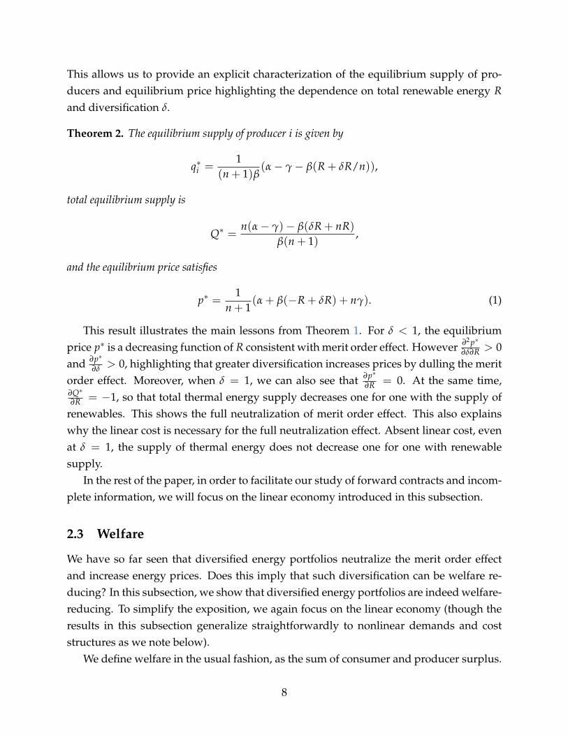
This allows us to provide an explicit characterization of the equilibrium supply of pro-ducers and equilibrium price highlighting the dependence on total renewable energy Rand diversification δ.
Theorem 2. The equilibrium supply of producer i is given by
q∗i =1
(n + 1)β(α− γ− β(R + δR/n)),
total equilibrium supply is
Q∗ =n(α− γ)− β(δR + nR)
β(n + 1),
and the equilibrium price satisfies
p∗ =1
n + 1(α + β(−R + δR) + nγ). (1)
This result illustrates the main lessons from Theorem 1. For δ < 1, the equilibriumprice p∗ is a decreasing function of R consistent with merit order effect. However ∂2 p∗
∂δ∂R > 0and ∂p∗
∂δ > 0, highlighting that greater diversification increases prices by dulling the meritorder effect. Moreover, when δ = 1, we can also see that ∂p∗
∂R = 0. At the same time,∂Q∗∂R = −1, so that total thermal energy supply decreases one for one with the supply of
renewables. This shows the full neutralization of merit order effect. This also explainswhy the linear cost is necessary for the full neutralization effect. Absent linear cost, evenat δ = 1, the supply of thermal energy does not decrease one for one with renewablesupply.
In the rest of the paper, in order to facilitate our study of forward contracts and incom-plete information, we will focus on the linear economy introduced in this subsection.
2.3 Welfare
We have so far seen that diversified energy portfolios neutralize the merit order effectand increase energy prices. Does this imply that such diversification can be welfare re-ducing? In this subsection, we show that diversified energy portfolios are indeed welfare-reducing. To simplify the exposition, we again focus on the linear economy (though theresults in this subsection generalize straightforwardly to nonlinear demands and coststructures as we note below).
We define welfare in the usual fashion, as the sum of consumer and producer surplus.
8
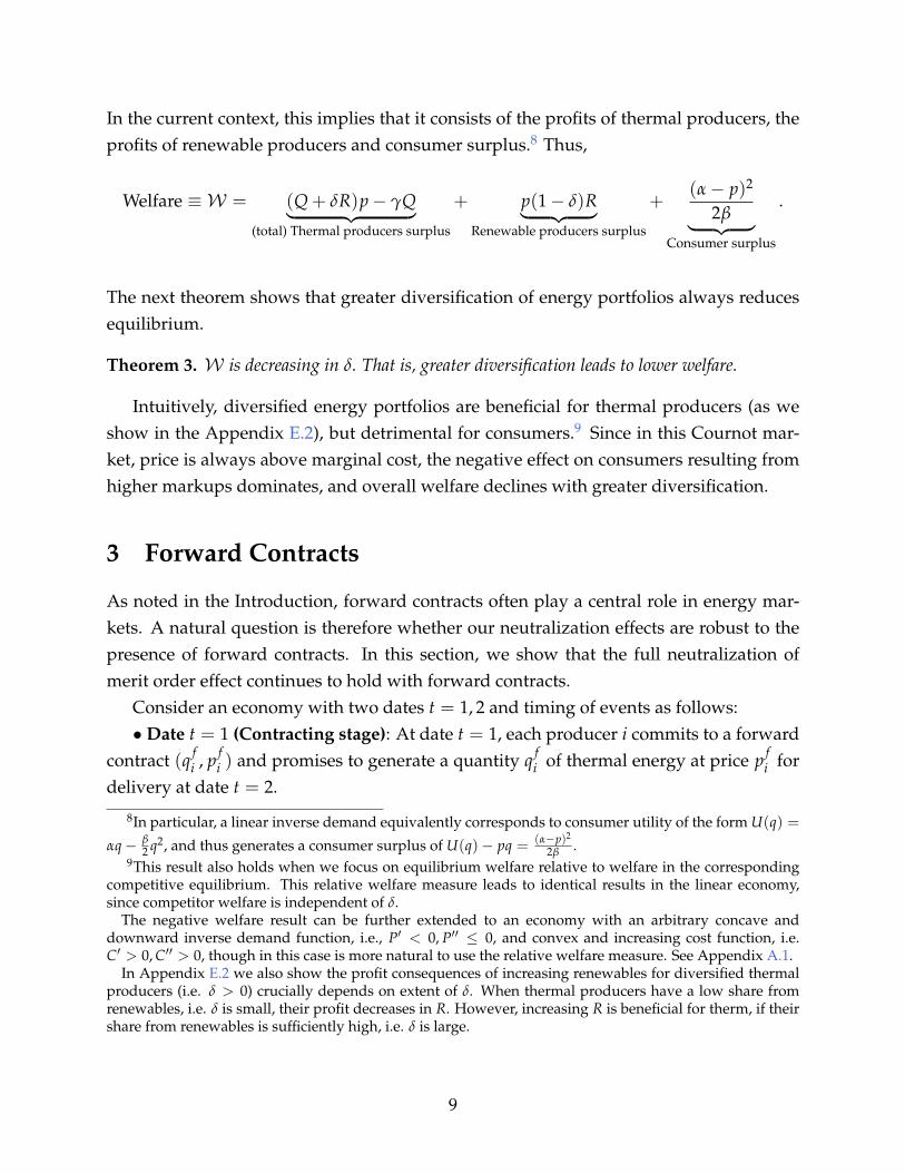
In the current context, this implies that it consists of the profits of thermal producers, theprofits of renewable producers and consumer surplus.8 Thus,
Welfare ≡ W = (Q + δR)p− γQ︸ ︷︷ ︸(total) Thermal producers surplus
+ p(1− δ)R︸ ︷︷ ︸Renewable producers surplus
+(α− p)2
2β︸ ︷︷ ︸Consumer surplus
.
The next theorem shows that greater diversification of energy portfolios always reducesequilibrium.
Theorem 3. W is decreasing in δ. That is, greater diversification leads to lower welfare.
Intuitively, diversified energy portfolios are beneficial for thermal producers (as weshow in the Appendix E.2), but detrimental for consumers.9 Since in this Cournot mar-ket, price is always above marginal cost, the negative effect on consumers resulting fromhigher markups dominates, and overall welfare declines with greater diversification.
3 Forward Contracts
As noted in the Introduction, forward contracts often play a central role in energy mar-kets. A natural question is therefore whether our neutralization effects are robust to thepresence of forward contracts. In this section, we show that the full neutralization ofmerit order effect continues to hold with forward contracts.
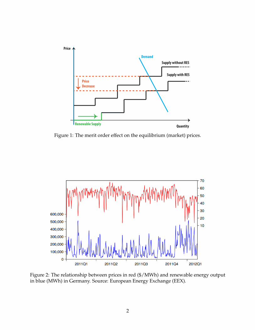
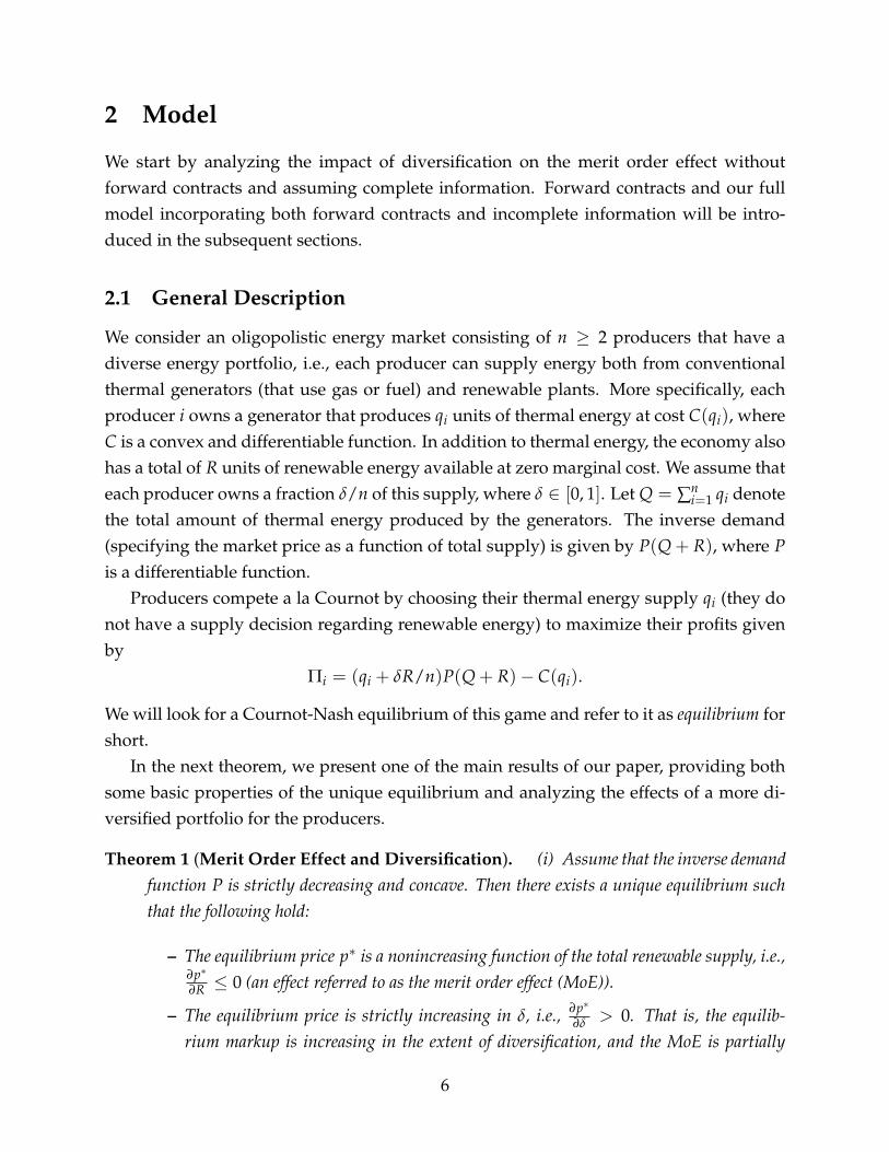
Consider an economy with two dates t = 1, 2 and timing of events as follows:• Date t = 1 (Contracting stage): At date t = 1, each producer i commits to a forward
contract (q fi , p f
i ) and promises to generate a quantity q fi of thermal energy at price p f
i fordelivery at date t = 2.
8In particular, a linear inverse demand equivalently corresponds to consumer utility of the form U(q) =
αq− β2 q2, and thus generates a consumer surplus of U(q)− pq = (α−p)2
2β .9This result also holds when we focus on equilibrium welfare relative to welfare in the corresponding
competitive equilibrium. This relative welfare measure leads to identical results in the linear economy,since competitor welfare is independent of δ.
The negative welfare result can be further extended to an economy with an arbitrary concave anddownward inverse demand function, i.e., P′ < 0, P′′ ≤ 0, and convex and increasing cost function, i.e.C′ > 0, C′′ > 0, though in this case is more natural to use the relative welfare measure. See Appendix A.1.
In Appendix E.2 we also show the profit consequences of increasing renewables for diversified thermalproducers (i.e. δ > 0) crucially depends on extent of δ. When thermal producers have a low share fromrenewables, i.e. δ is small, their profit decreases in R. However, increasing R is beneficial for therm, if theirshare from renewables is sufficiently high, i.e. δ is large.
9
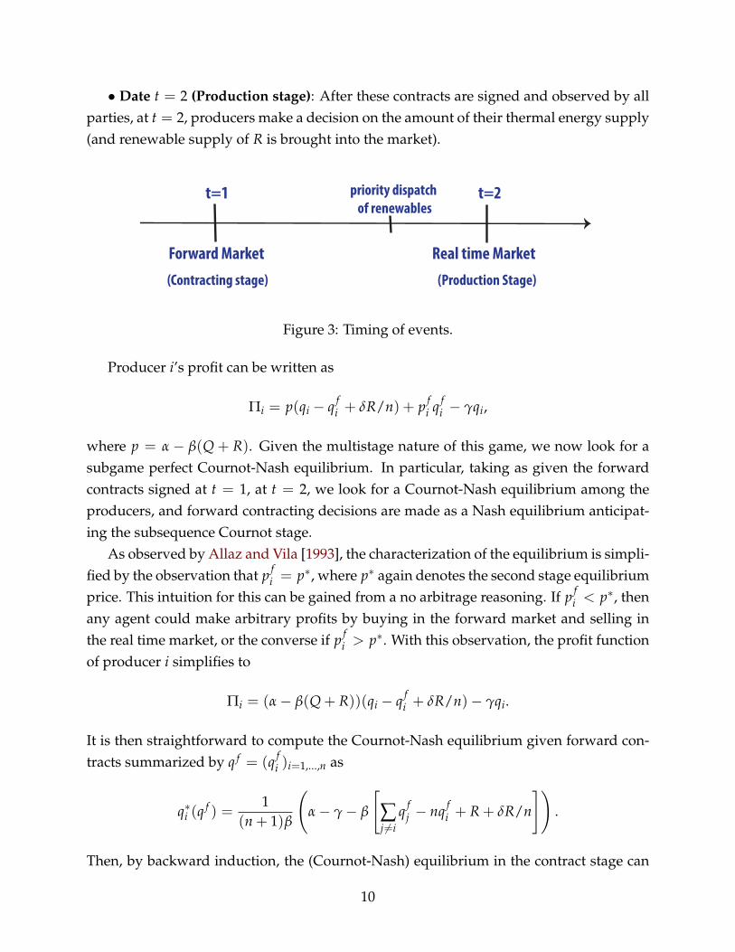
• Date t = 2 (Production stage): After these contracts are signed and observed by allparties, at t = 2, producers make a decision on the amount of their thermal energy supply(and renewable supply of R is brought into the market).
t=1 t=2
Forward Market
(Contracting stage)
Real time Market
(Production Stage)
priority dispatch
of renewables
Figure 3: Timing of events.
Producer i’s profit can be written as
Πi = p(qi − q fi + δR/n) + p f
i q fi − γqi,
where p = α− β(Q + R). Given the multistage nature of this game, we now look for asubgame perfect Cournot-Nash equilibrium. In particular, taking as given the forwardcontracts signed at t = 1, at t = 2, we look for a Cournot-Nash equilibrium among theproducers, and forward contracting decisions are made as a Nash equilibrium anticipat-ing the subsequence Cournot stage.
As observed by Allaz and Vila [1993], the characterization of the equilibrium is simpli-fied by the observation that p f
i = p∗, where p∗ again denotes the second stage equilibriumprice. This intuition for this can be gained from a no arbitrage reasoning. If p f
i < p∗, thenany agent could make arbitrary profits by buying in the forward market and selling inthe real time market, or the converse if p f
i > p∗. With this observation, the profit functionof producer i simplifies to
Πi = (α− β(Q + R))(qi − q fi + δR/n)− γqi.
It is then straightforward to compute the Cournot-Nash equilibrium given forward con-tracts summarized by q f = (q f
i )i=1,...,n as
q∗i (qf ) =
1(n + 1)β
(α− γ− β
[∑j 6=i
q fj − nq f
i + R + δR/n
]).
Then, by backward induction, the (Cournot-Nash) equilibrium in the contract stage can
10
be determined as the fixed point of the best response correspondences characterized by
q∗ fi ∈ arg max
q fi ≥0
{p(
q∗i (qfi , q∗ f−i) + δR/n
)− γq∗i (q
fi , q∗ f−i)}
s.t. p = α− β(Q∗(q fi , q∗ f−i) + R),
where Q∗(q fi , q∗ f−i) is the total supply given the forward contracts (q f
i , q∗ f−i).
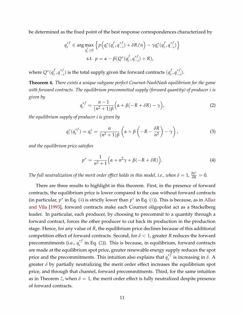
Theorem 4. There exists a unique subgame perfect Cournot-NashNash equilibrium for the gamewith forward contracts. The equilibrium precommitted supply (forward quantity) of producer i isgiven by
q∗ fi =
n− 1(n2 + 1)β
(α + β(−R + δR)− γ
), (2)
the equilibrium supply of producer i is given by
q∗i (q∗ fi ) = q∗i =
n(n2 + 1)β
(α + β
(−R− δR
n2
)− γ
), (3)
and the equilibrium price satisfies
p∗ =1
n2 + 1
(α + n2γ + β(−R + δR)
). (4)
The full neutralization of the merit order effect holds in this model, i.e., when δ = 1, ∂p∗∂R = 0.
There are three results to highlight in this theorem. First, in the presence of forwardcontracts, the equilibrium price is lower compared to the case without forward contracts(in particular, p∗ in Eq. (4) is strictly lower than p∗ in Eq. (1)). This is because, as in Allazand Vila [1993], forward contracts make each Cournot oligopolist act as a Stackelbergleader. In particular, each producer, by choosing to precommit to a quantity through aforward contract, forces the other producer to cut back its production in the productionstage. Hence, for any value of R, the equilibrium price declines because of this additionalcompetition effect of forward contracts. Second, for δ < 1, greater R reduces the forwardprecommitments (i.e., q∗ f
i in Eq. (2)). This is because, in equilibrium, forward contractsare made at the equilibrium spot price, greater renewable energy supply reduces the spotprice and the precommitments. This intuition also explains that q∗ f
i is increasing in δ. Agreater δ by partially neutralizing the merit order effect increases the equilibrium spotprice, and through that channel, forward precommitments. Third, for the same intuitionas in Theorem 2, when δ = 1, the merit order effect is fully neutralized despite presenceof forward contracts.
11
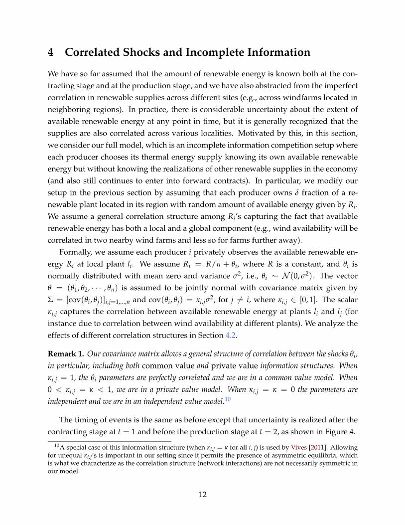
4 Correlated Shocks and Incomplete Information
We have so far assumed that the amount of renewable energy is known both at the con-tracting stage and at the production stage, and we have also abstracted from the imperfectcorrelation in renewable supplies across different sites (e.g., across windfarms located inneighboring regions). In practice, there is considerable uncertainty about the extent ofavailable renewable energy at any point in time, but it is generally recognized that thesupplies are also correlated across various localities. Motivated by this, in this section,we consider our full model, which is an incomplete information competition setup whereeach producer chooses its thermal energy supply knowing its own available renewableenergy but without knowing the realizations of other renewable supplies in the economy(and also still continues to enter into forward contracts). In particular, we modify oursetup in the previous section by assuming that each producer owns δ fraction of a re-newable plant located in its region with random amount of available energy given by Ri.We assume a general correlation structure among Ri’s capturing the fact that availablerenewable energy has both a local and a global component (e.g., wind availability will becorrelated in two nearby wind farms and less so for farms further away).
Formally, we assume each producer i privately observes the available renewable en-ergy Ri at local plant li. We assume Ri = R/n + θi, where R is a constant, and θi isnormally distributed with mean zero and variance σ2, i.e., θi ∼ N (0, σ2). The vectorθ = (θ1, θ2, · · · , θn) is assumed to be jointly normal with covariance matrix given byΣ = [cov(θi, θj)]i,j=1,...,n and cov(θi, θj) = κi,jσ
2, for j 6= i, where κi,j ∈ [0, 1]. The scalarκi,j captures the correlation between available renewable energy at plants li and lj (forinstance due to correlation between wind availability at different plants). We analyze theeffects of different correlation structures in Section 4.2.
Remark 1. Our covariance matrix allows a general structure of correlation between the shocks θi,in particular, including both common value and private value information structures. Whenκi,j = 1, the θi parameters are perfectly correlated and we are in a common value model. When0 < κi,j = κ < 1, we are in a private value model. When κi,j = κ = 0 the parameters areindependent and we are in an independent value model.10
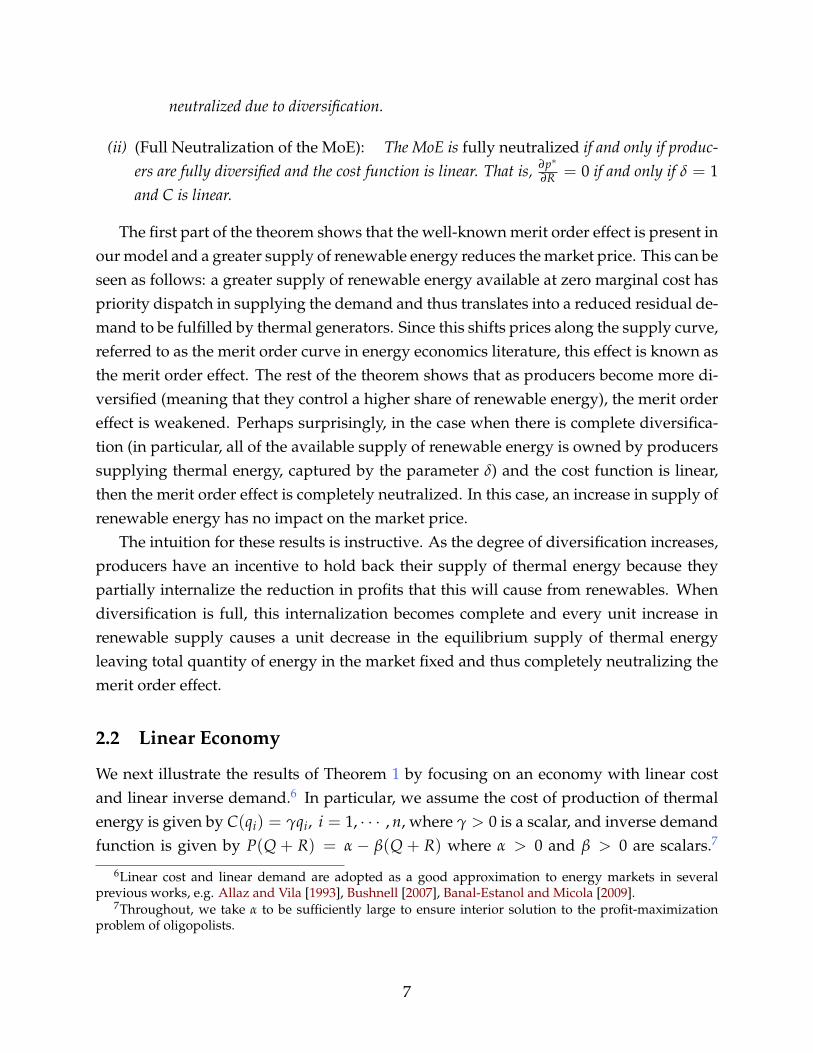
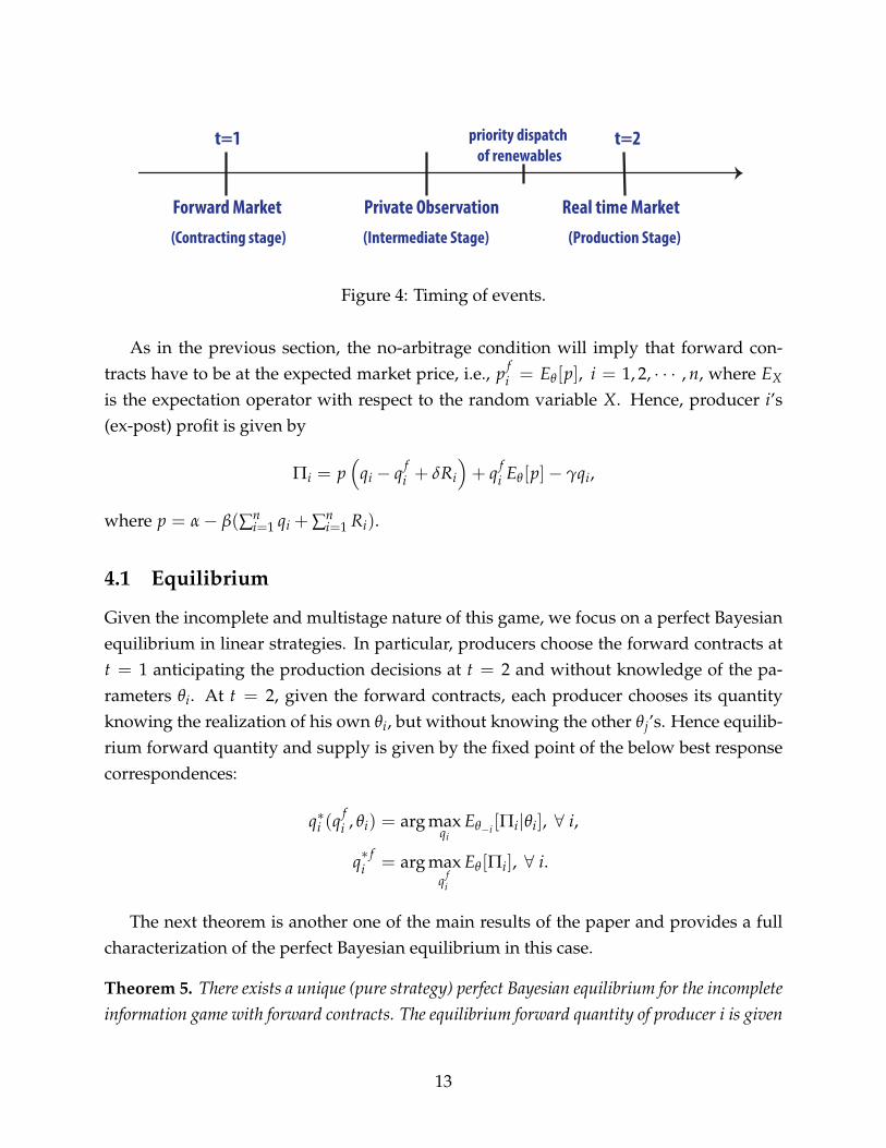
The timing of events is the same as before except that uncertainty is realized after thecontracting stage at t = 1 and before the production stage at t = 2, as shown in Figure 4.
10A special case of this information structure (when κi,j = κ for all i, j) is used by Vives [2011]. Allowingfor unequal κi,j’s is important in our setting since it permits the presence of asymmetric equilibria, whichis what we characterize as the correlation structure (network interactions) are not necessarily symmetric inour model.
12
t=1 t=2
Forward Market
(Contracting stage)
Real time Market
(Production Stage)
priority dispatch
of renewables
Private Observation
(Intermediate Stage)
Figure 4: Timing of events.
As in the previous section, the no-arbitrage condition will imply that forward con-tracts have to be at the expected market price, i.e., p f
i = Eθ[p], i = 1, 2, · · · , n, where EX
is the expectation operator with respect to the random variable X. Hence, producer i’s(ex-post) profit is given by
Πi = p(
qi − q fi + δRi
)+ q f
i Eθ[p]− γqi,
where p = α− β(∑ni=1 qi + ∑n
i=1 Ri).
4.1 Equilibrium
Given the incomplete and multistage nature of this game, we focus on a perfect Bayesianequilibrium in linear strategies. In particular, producers choose the forward contracts att = 1 anticipating the production decisions at t = 2 and without knowledge of the pa-rameters θi. At t = 2, given the forward contracts, each producer chooses its quantityknowing the realization of his own θi, but without knowing the other θj’s. Hence equilib-rium forward quantity and supply is given by the fixed point of the below best responsecorrespondences:
q∗i (qfi , θi) = arg max
qiEθ−i [Πi|θi], ∀ i,
q∗ fi = arg max
q fi
Eθ[Πi], ∀ i.
The next theorem is another one of the main results of the paper and provides a fullcharacterization of the perfect Bayesian equilibrium in this case.
Theorem 5. There exists a unique (pure strategy) perfect Bayesian equilibrium for the incompleteinformation game with forward contracts. The equilibrium forward quantity of producer i is given
13
by
q∗ fi =
n− 1(n2 + 1)β
(α + β(−R + δR)− γ
)(5)
and the equilibrium supply of producer i (as a function of the parameter θi) is given by
q∗i (θi) =n
(n2 + 1)β
(α + β
(−R− δR
n2
)− γ
)− aiθi (6)
where a1
a2...
an
= 1 + (δ− 1)(
I +1σ2 Σ
)−1
1,
where 1 and I denote the vector of all ones and the identity matrix, respectively. Moreover theexpected value of the equilibrium price is given by
E[p∗] =1
n2 + 1
(α + n2γ + β(−R + δR)
).
The full neutralization of the merit order effect holds in this model, i.e., when δ = 1, ∂E[p∗]∂R = 0.
Remark 2. It follows from the preceding characterization of the equilibrium that in the indepen-dent value model where κi,j = 0 for all i 6= j, a1 = a2 = · · · = an = 1+δ
2 and, in the commonvalue model where κi,j = κ ∈ (0, 1) for all i 6= j, a1 = a2 = · · · = an = 1+δ+(n−1)κ
2+(n−1)κ .
Even though the structure of equilibria becomes richer in the presence of incompleteinformation (and we will discuss some of the properties of this equilibrium in more detailbelow), the results on the impact of the renewable supply and the extent of diversificationof producers mimics Theorems 2 and 4. When δ < 1, a greater supply of renewablesreduces expected equilibrium price due to merit order effect (and for the same reasonas in Theorem 4, it reduces q f ∗), and greater δ increases expected equilibrium price (andtends to increase q f ∗). In addition, when δ = 1, the neutralization of the merit order effectis complete and expected equilibrium price is independent of R.
We can also observe the impact of private information θi on the quantity choices ofproducers. In particular, a higher θi reduces the quantity supplied because producer iitself has access to greater renewables and given the correlation across θi’s, also expectsothers to have greater renewables creating another force towards lower supply through
14
the strategic substitutes effect in Cournot competition. It is the combination of these forcesthat make the coefficient in front of θi, ai, depend on both δ (the extent of diversification)and the correlation structure of θi’s as in Eq. (6).
Example (duopoly with forward contracts and incomplete information) To high-light the effect of the correlation among the parameters θi on equilibrium, we focus on thespecial case with two producers. We assume Cov(θ1, θ2) = κσ2, where κ is a parameterthat scales inversely with the distance among the renewable plants of the producers. Us-ing Theorem 5, we have a unique perfect Bayesian Nash equilibrium in linear strategies.The equilibrium supply of producer i is given by
q∗i (θi) =2
5β(α + β(−R− δR/4)− γ)−
(1 + δ + κ
2 + κ
)θi
= q∗i −(
1 + δ + κ
2 + κ
)θi, (7)
where q∗i is the equilibrium of the same economy with complete information. The equi-librium price satisfies
E[p∗] =15(α + β(−R + δR) + 4γ).
Intuitively, similar to the previous cases, at equilibrium, each producer cuts back onits thermal supply in response to an increase in the renewable supply (given by θi) dueto the strategic substitutes effect in Cournot competition. This reduction is modulatedsince renewable energy availability is now correlated among different plants (i.e., whenmy renewable energy is high, so is my competitor’s) and this creates incentive for greaterholding back.11 Most interestingly, when δ = 1, this modulation disappears and pro-duction becomes independent of κ. This is again an implication of the neutralization ofmerit order effect. When δ = 1, total production of each producer i (thermal+renewable)is independent of the parameter θi. Since his competitor’s production is independent ofhis private information, the correlation between their θ’s does not impact the producer’ssupply decision.
4.2 Price volatility
The next proposition provides a characterization of price volatility and highlights its de-pendence on renewable share of producers δ and the correlation structure among param-eters θi.
11This is because 1+δ+κ2+κ is increasing in κ.
15
Proposition 1. The equilibrium price volatility is given by
Var(p∗) = β2(δ− 1)2 bTΣb, (8)
where b ≡(
I + 1σ2 Σ)−1
1.12 When producers are fully diversified (they have full ownership ofrenewable supply), price volatility disappears, i.e., when δ = 1, Var(p) = 0.
This proposition shows that price volatility decreases when the share of producersfrom renewable supply increases, i.e. ∂Var(p)
∂δ < 0, and it disappears when δ = 1. Thisis again due to the fact that when producers have full ownership of all renewable sup-ply (i.e., δ = 1), the total supply (via thermal and renewable sources) of each produceri becomes independent of his type θi, vanishing price volatility, i.e., when δ = 1 thenVar(p) = 0.
The following table summarizes the effect of diversification on the equilibrium price,price volatility and equilibrium forward quantity.
equilibrium price price volatility forward quantity
Renewable outcome (R ↑) − + −Diversification (δ ↑) + − +
δ = 1 N N N
Table 1: The effect of renewable energy (R) on equilibrium price (p∗), price volatilityVar(p∗) and equilibrium forward quantity (q f ). With full diversification, all three quanti-ties become independent of R, which we denote by N in the table.
We next investigate the impact of correlation structure among parameters θi on pricevolatility. Since correlation among θi’s captures correlation among renewable energyavailability at different plants, our analysis reveals the effect of any kind of dependency,e.g. spatial configuration, of renewable plants on price volatility. We focus on regularconfiguration in the next section. Price volatility for non-regular structures is studied inAppendix, Section F.
12The vector b is referred to as the Bonacich centrality vector in network models and measures the nodes’centralities in a weighted graph where the weighs in this case are given by the entires of the covariancematrix Σ (see Ballester et al. [2006], Jackson [2008], Acemoglu et al. [2012], Candogan et al. [2012], Bramoulléet al. [2014]).
16
4.3 Regular Configurations
We next focus on regular configurations, corresponding to a symmetric correlation struc-ture for the renewable plants. This is defined formally through the covariance matrix ofθ1, θ2, · · · , θn as follows.
Definition 1 (Regular configurations). Renewable plants have a regular configuration if thecovariance matrix Σ is row-(sub)stochastic. That is, ∑n
j 6=i κi,j = K, where K is fixed and the samefor all i = 1, 2, · · · , n.
Hence, regular configurations represent a correlation structure in which the total co-variance of each θi with other θj’s is the same. It follows from Theorem 5 that for regularconfigurations, the equilibrium is symmetric, i.e., a1 = · · · = an. Thus, the price volatilitycan be characterized explicitly in terms of K as follows.
Lemma 6. The price volatility of any regular configuration is given by
Var(p) = nσ2β2(
1− δ
2 + K
)2
(1 + K). (9)
Var(p) is decreasing in K, i.e., ∂Var(p)∂K < 0.
This lemma shows that the price volatility increases when the overall correlation ofeach plant with its neighbors (i.e. K) decreases. This is intuitive since decreasing thetotal correlation creates more miscoordination in supplies across producers, increasingvolatility in aggregate production. Thus, price volatility rises with decreasing K.
Remark 3. This monotonicity of price volatility in K depends on the extent of convexity in the costfunction. When the cost function is highly convex, price volatility can increase with K. This canbe seen by considering the case where the cost function, C(qi), is sufficiently convex so that severalproducers rely increasingly on their renewable supply (i.e. qi(θi) becomes small). As a result, theaggregate production in the economy mostly comes form the aggregate renewable supply. That is
Aggregate production =n
∑i=1
qi(θ) +n
∑i=1
Ri ≈n
∑i=1
Ri = R +n
∑i=1
θi,
where R is constant. Hence, greater correlation, i.e. K, increases Var(∑ni=1 θi) = 1TΣ1 =
nσ2(1 + K), increasing volatility in the aggregate production. Thus, price volatility rises withincreasing K (see Theorem 8 in Appendix A.2).
We next present two extreme cases of regular models and consider their implicationson the market price volatility.
17
1
2
3
n
1
2
3
n
Figure 5: Circle model and complete model.
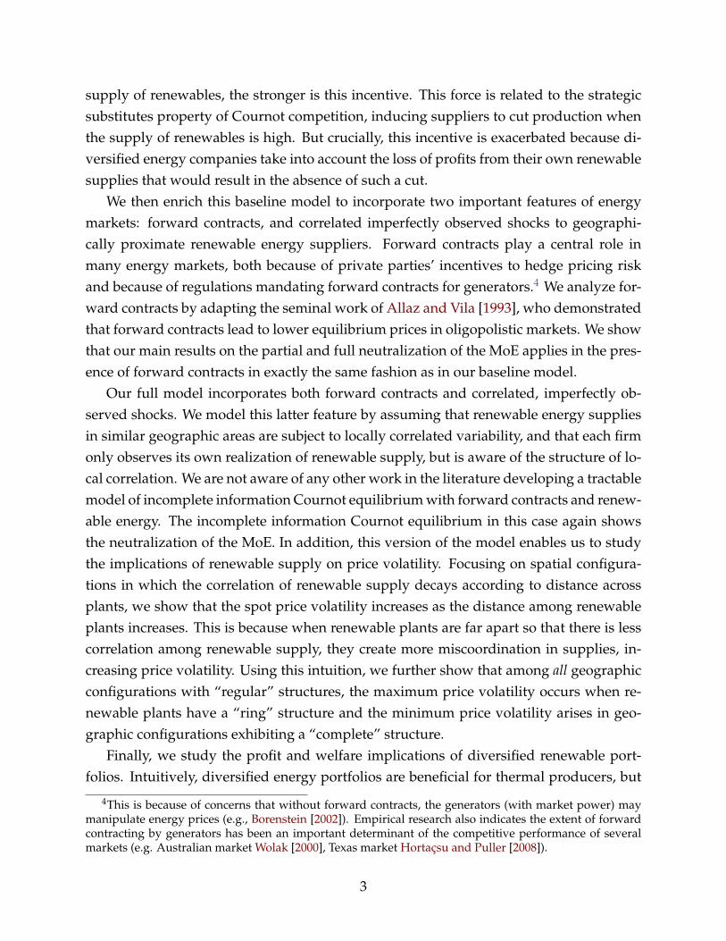
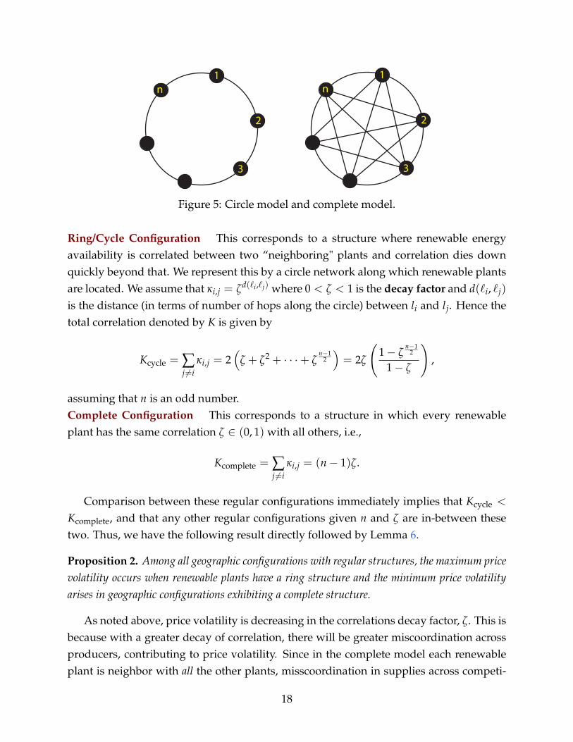
Ring/Cycle Configuration This corresponds to a structure where renewable energyavailability is correlated between two “neighboring" plants and correlation dies downquickly beyond that. We represent this by a circle network along which renewable plantsare located. We assume that κi,j = ζd(`i,`j) where 0 < ζ < 1 is the decay factor and d(`i, `j)
is the distance (in terms of number of hops along the circle) between li and lj. Hence thetotal correlation denoted by K is given by
Kcycle = ∑j 6=i
κi,j = 2(
ζ + ζ2 + · · ·+ ζn−1
2
)= 2ζ
(1− ζ
n−12
1− ζ
),
assuming that n is an odd number.Complete Configuration This corresponds to a structure in which every renewableplant has the same correlation ζ ∈ (0, 1) with all others, i.e.,
Kcomplete = ∑j 6=i
κi,j = (n− 1)ζ.
Comparison between these regular configurations immediately implies that Kcycle <
Kcomplete, and that any other regular configurations given n and ζ are in-between thesetwo. Thus, we have the following result directly followed by Lemma 6.
Proposition 2. Among all geographic configurations with regular structures, the maximum pricevolatility occurs when renewable plants have a ring structure and the minimum price volatilityarises in geographic configurations exhibiting a complete structure.
As noted above, price volatility is decreasing in the correlations decay factor, ζ. This isbecause with a greater decay of correlation, there will be greater miscoordination acrossproducers, contributing to price volatility. Since in the complete model each renewableplant is neighbor with all the other plants, misscoordination in supplies across competi-
18
tors is lower than any other regular geographic configurations. The converse holds forthe ring structures, where each renewable plant is neighbor with only two plants. Thus,the maximum price volatility occurs when renewable plants have a ring structure andthe minimum price volatility arises in geographic configurations exhibiting a completestructure. Price volatility in any other regular configuration lies between these two polarcases.13
5 Conclusion
With mounting concerns over climate change caused by fossil fuels, there has been grow-ing reliance on renewable energy. Many countries have responded by not only intro-ducing renewable energy policy targets for the economy at large but imposing these onconventional energy companies. The hope has been to both reduce fossil fuel emissionsand also benefit from renewable energy by offering lower prices to consumers throughthe merit order effect, which refers to the negative impact of renewables, typically supplythat low marginal cost, on energy prices.
This paper has studied the implications of diversified energy portfolios on equilibriumprices and the merit order effect in an oligopolistic energy market, and has suggested thatthe two aforementioned objectives of renewable energy policy may be contradictory. Wehave shown, in particular, that when thermal generators have a diverse energy portfolio,meaning that they also control some or all of renewable supplies, they offset the pricedeclines due to the merit order effect because they strategically reduce their conventionalenergy supplies when renewable supply is high. In the limit case where all renewablesupply is controlled by thermal power generators this offset is complete — meaning thatthe merit order effect is totally neutralized and renewable supplies have no impact onmarket prices. We also established that, through this neutralization of the merit order ef-fect and the resulting higher markups, diversified energy portfolios are welfare-reducing.
These results are first derived in the baseline Cournot model oligopolistic competition.They are then extended to a setup with forward contracts and with incomplete informa-tion about imperfectly correlated shocks affecting renewable supplies across the generalgeographic landscape. In addition to showing the robustness of the partial and full neu-tralization of the merit order effect, we have used our general framework to study theimplications of different calculations on price volatility.
13Given the definition of regular structures, for any k-regular configuration with n renewable plants,K(n,2)
cycle < K(n,k)regular < K(n,n−1)
complete.
19
References
D. Acemoglu, V. Carvalho, A. Ozdaglar, and A. Tahbaz-Salehi. The network origins ofaggregate fluctuations. Econometrica, 80(5):1977–2016, 2012.
B. Allaz and J.-L. Vila. Cournot competition, forward markets and efficiency. Journal ofEconomic Theory, 59(1):1–16, 1993.
R. Baldick and W. W. Hogan. Capacity constrained supply function equilibrium models ofelectricity markets: Stability, non-decreasing constraints, and function space iterations.Mimeo, 2002.
R. Baldick, R. Grant, and E. Kahn. Theory and application of linear supply functionequilibrium in electricity markets. Journal of Regulatory Economics, 25(2):143–167, 2004.
C. Ballester, A. Calvó-Armengol, and Y. Zenou. Who’s who in networks. wanted: The keyplayer. Econometrica, 74(5):1403–1417, 2006.
A. Banal-Estanol and A. R. Micola. Composition of electricity generation portfolios, piv-otal dynamics, and market prices. Management Science, 55(11):1813–1831, 2009.
O. Ben-Moshe and O. D. Rubin. Does wind energy mitigate market power in deregulatedelectricity markets? Energy, forthcoming.
E. Y. Bitar, R. Rajagopal, P. P. Khargonekar, K. Poolla, and P. P. Varaiya. Bringing windenergy to market. IEEE Transactions on Power Systems, 27(3):1225–1235, 2012.
S. Borenstein. The trouble with electricity markets: Understanding california’s restructur-ing disaster. Journal of Economic Perspectives, 16(1):191–211, 2002.
S. Borenstein and J. Bushnell. An empirical analysis of the potential for market power incalifornia’s electricity industry. Journal of Industrial Economics, 47(3):285–323, 1999.
S. Borenstein, J. Bushnell, E. Kahn, and S. Stoft. Market power in california electricitymarkets. Utilities Policy, 5(3/4):219–236, 1995.
S. Borenstein, J. Bushnell, and C. R. Knittel. Market power in electricity markets: Beyondconcentration measures. Energy Journal, 20(4):65–88, 1999.
S. Bose, D. Cai, S. Low, and A. Wierman. The role of a market maker in networked cournotcompetition. Working paper, 2014.
20
Y. Bramoullé, R. Kranton, and M. D’Amours. Strategic interaction and networks. AmericanEconomic Review, 104(3):898–930, 2014.
J. Bushnell. Oligopoly equilibria in electricity contract markets. Journal of Regulatory Eco-nomics, 32(2):225–245, 2007.
O. Candogan, K. Bimpikis, and A. Ozdaglar. Optimal pricing in networks with externali-ties. Operations Research, 60(4):883–905, 2012.
J. Cludiusa, H. Hermannb, F. C. Matthesb, and V. Graichen. The merit order effect of windand photovoltaic electricity generation in germany 2008-2016 estimation and distribu-tional implications. Energy Economics, forthcoming, 2014.
M. H. DeGroot. Optimal Statistical Decisions. John Wiley and Sons (Wiley Classics LibraryEdition), 1970.
I. Dincer. Renewable energy and sustainable development: a crucial review. Renewableand Sustainable Energy Reviews, 4(2):157–175, 2000.
T. Downward, G. Zakeri, and A. Philpott. On cournot equilibria in electricity transmissionnetworks. Operation Research, 58(4):1194–1209, 2010.
J. L. Ferreira. Strategic interaction between futures and spot markets. Journal of EconomicTheory, 108(1):141–151, 2003.
R. Green. The electricity contract market in england and wales. Journal of Industrial Eco-nomics, 47(1):107–124, 1999.
R. Green and C. L. Coq. The length of the contract and collusion. International Journal ofIndustrial Organization, 28(1):21–29, 2010.
R. J. Green and D. M. Newbery. Competition in the british electricity spot market. Journalof Political Economy, 100(5):929–953, 1992.
W. W. Hogan. A market power model with strategic interaction in electricity networks.Energy Journal, 18(4):107–141, 1997.
A. Hortaçsu and S. L. Puller. Understanding strategic bidding in multi-unit auctions: acase study of the texas electricity spot market. The RAND Journal of Economics, 39(2):86–114, 2008.
J. Hughes and J. L. Kao. Strategic forward contracting and observability. InternationalJournal of Industrial Organization, 16(1):121–33, 1997.
21
M. O. Jackson. Social and Economic Networks. Princeton University Press, Princeton, NJ.,2008.
P. L. Joskow. Deregulation and regulatory reform in the u.s. electric power sector. Mimeo,2001.
J. H. Kim and W. B. Powell. Optimal energy commitments with storage and intermittentsupply. Operation Research, 59(6):1347–1360, 2011.
P. D. Klemperer and M. A. Meyer. Supply function equilibria in oligopoly under uncer-tainty. Econometrica, 57(6):1243–1277, 1989.
C. D. Kolstad and L. Mathiesen. Necessary and sufficient conditions for uniqueness of acournot equilibrium. Review of Economic Studies, 54(4):681–690, 1987.
M. Korpaas, A. T. Holen, and R. Hildrum. Operation and sizing of energy storage forwind power plants in a market system. International Journal of Electrical Power & EnergySystems, 25(8):599–606, 2003.
S. Lalwani and J. Khoo. A diverse energy portfolio is the answer to this century’senergy trilemma, says alstom at the world energy congress 2013. Available athttp://www.alstom.com/press-centre, 2013.
M. Liski and J.-P. Montero. Forward trading and collusion in oligopoly. Journal of EconomicTheory, 131(1):212–230, 2006.
P. Mahenc and F. Salanie. Softening competition through forward trading. Journal ofEconomic Theory, 116(2):282–293, 2004.
D. McConnella, P. Hearpsa, D. Ealesb, M. Sandiforda, R. Dunnc, M. Wrightb, and L. Bate-mand. Retrospective modeling of the merit-order effect on wholesale electricity pricesfrom distributed photovoltaic generation in the australian national electricity market.Energy Policy, 58:17–27, 2013.
S. Meyn, M. Negrete-Pincetic, G. Wang, A. Kowli, and E. Shafieepoorfard. The value ofvolatile resources in electricity markets. 49th IEEE Conference on Decision and Control,pages 1029–1036, 2010.
J. Munksgaarda and P. E. Morthorstb. Wind power in the danish liberalised powermarket–policy measures, price impact and investor incentives. Energy Policy, 36(10):3940–3947, 2008.
22
J. Nair, S. Adlakha, and A. Wierman. Energy procurement strategies in the presence ofintermittent sources. Proceedings of ACM Sigmetrics, 2014.
M. Nicolosi and M. Fursch. The impact of an increasing share of res-e on the conventionalpower market: The example of germany. Z. Energiewirtschaft, 33(3):246–254., 2009.
A. O’Mahoney and D. Eleanor. The merit order effect of wind generation on the irishelectricity market. Working paper, 2011.
S. Oren. Economic inefficiency of passive transmission rights in congested electrical sys-tem with competitive generation. Energy Journal, 18(1):63–83, 1997.
R. Rajagopal, E. Y. Bitar, F. Wu, and P. P. Varaiya. Risk limiting dispatch of wind power.American Control Conference, pages 4417–4422, 2012.
A. Rudkevich, M. Duckworth, and R. Rosen. Modeling electricity pricing in a deregulatedgeneration industry: the potential for oligopoly pricing in a poolco. Energy Journal, 19(3):19–48, 1998.
T. Scott and E. Read. Modeling hydro reservoir operation in a deregulated electricitymarket. International Transactions in Operational Research, 3(5):243–253, 1996.
F. Sensfuss, M. Ragwitz, and M. Genoese. The merit-order effect: A detailed analysis ofthe price effect of renewable electricity generation on spot market in germany. EnergyPolicy, 36(8):3086–3094, 2008.
U.S. Energy Information Administration. Direct federal financial interventions and sub-sidies in energy in fiscal year 2013. Final report, 2013.
P. P. Varaiya, F. F. Wu, and J. W. Bialek. Smart operation of smart grid: Risk-limitingdispatch. Proceedings of the IEEE, 99(1):40–57, 2011.
M. Ventosa, A. R. A. Baill, and M. Rivier. Electricity market modeling trends. EnergyPolicy, 33(7):897–913, 2005.
X. Vives. Oligopoly Pricing: Old ideas and new tools. MIT Press, 1999.
X. Vives. Strategic supply function competition with private information. Econometrica,79(6):1919–1966, 2011.
B. Willems, I. Rumiantseva, and H. Weigt. Cournot versus supply functions: What doesthe data tell us? Energy Economics, 31(1):38–47, 2009.
23
F. A. Wolak. An empirical analysis of the impact of hedge contracts on bidding behaviorin a competitive electricity market. International Economic Journal, 14(2):1–39, 2000.
K. Wurzburg, X. Labandeira, and P. Linares. Renewable generation and electricity prices:Taking stock and new evidence for germany and austria. Energy Economics, 40:S159–S171, 2013.
J. Yao, I. Adler, and S. S. Oren. Modeling and computing two-settlement oligopolisticequilibrium in a congested electricity network. Operation Research, 56(1):34–46, 2008.
24
Appendix
A Extra results and Extensions
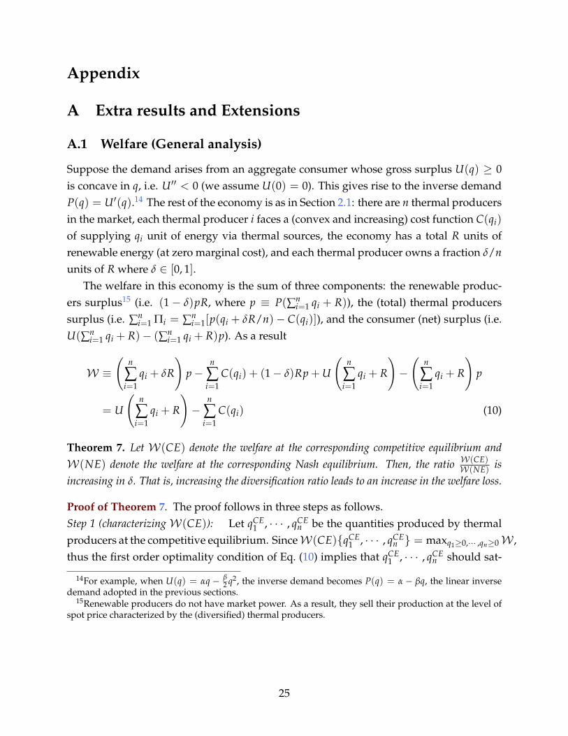
A.1 Welfare (General analysis)
Suppose the demand arises from an aggregate consumer whose gross surplus U(q) ≥ 0is concave in q, i.e. U′′ < 0 (we assume U(0) = 0). This gives rise to the inverse demandP(q) = U′(q).14 The rest of the economy is as in Section 2.1: there are n thermal producersin the market, each thermal producer i faces a (convex and increasing) cost function C(qi)
of supplying qi unit of energy via thermal sources, the economy has a total R units ofrenewable energy (at zero marginal cost), and each thermal producer owns a fraction δ/nunits of R where δ ∈ [0, 1].
The welfare in this economy is the sum of three components: the renewable produc-ers surplus15 (i.e. (1− δ)pR, where p ≡ P(∑n
i=1 qi + R)), the (total) thermal producerssurplus (i.e. ∑n
i=1 Πi = ∑ni=1[p(qi + δR/n)− C(qi)]), and the consumer (net) surplus (i.e.
U(∑ni=1 qi + R)− (∑n
i=1 qi + R)p). As a result
W ≡(
n
∑i=1
qi + δR
)p−
n
∑i=1
C(qi) + (1− δ)Rp + U
(n
∑i=1
qi + R
)−(
n
∑i=1
qi + R
)p
= U
(n
∑i=1
qi + R
)−
n
∑i=1
C(qi) (10)
Theorem 7. Let W(CE) denote the welfare at the corresponding competitive equilibrium andW(NE) denote the welfare at the corresponding Nash equilibrium. Then, the ratio W(CE)
W(NE) isincreasing in δ. That is, increasing the diversification ratio leads to an increase in the welfare loss.
Proof of Theorem 7. The proof follows in three steps as follows.Step 1 (characterizingW(CE)): Let qCE
1 , · · · , qCEn be the quantities produced by thermal
producers at the competitive equilibrium. SinceW(CE){qCE1 , · · · , qCE
n } = maxq1≥0,··· ,qn≥0W ,thus the first order optimality condition of Eq. (10) implies that qCE
1 , · · · , qCEn should sat-
14For example, when U(q) = αq− β2 q2, the inverse demand becomes P(q) = α− βq, the linear inverse
demand adopted in the previous sections.15Renewable producers do not have market power. As a result, they sell their production at the level of
spot price characterized by the (diversified) thermal producers.
25
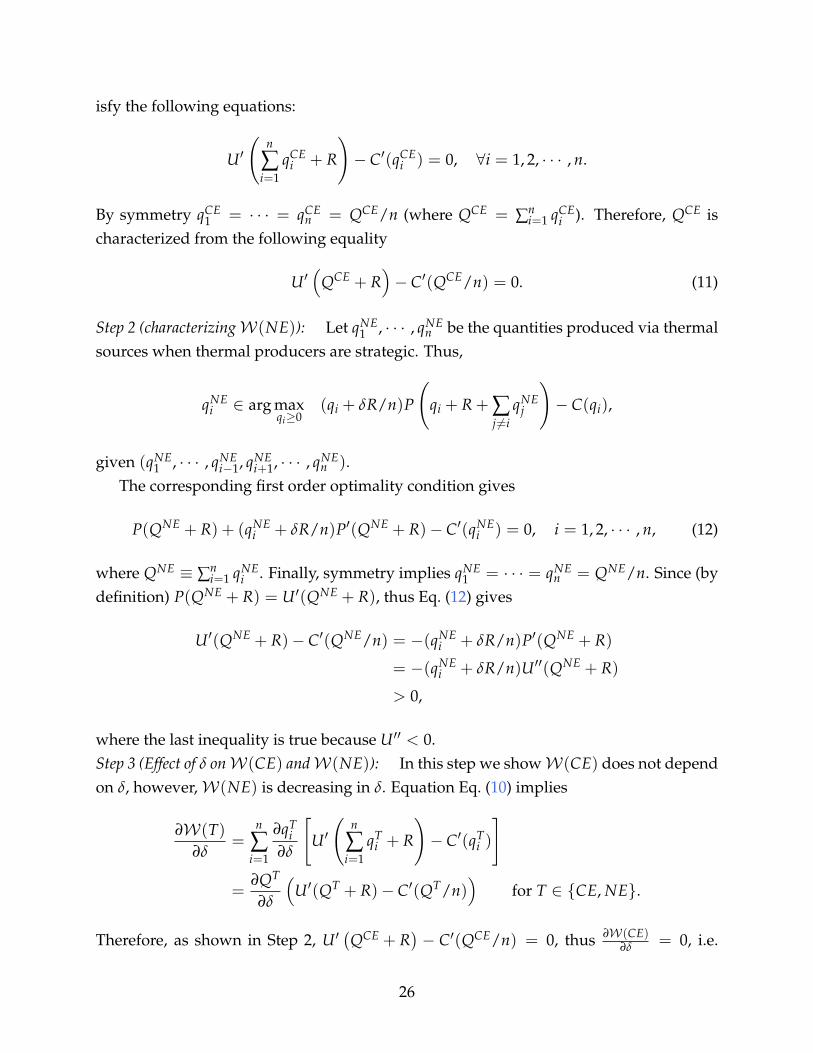
isfy the following equations:
U′(
n
∑i=1
qCEi + R
)− C′(qCE
i ) = 0, ∀i = 1, 2, · · · , n.
By symmetry qCE1 = · · · = qCE
n = QCE/n (where QCE = ∑ni=1 qCE
i ). Therefore, QCE ischaracterized from the following equality
U′(
QCE + R)− C′(QCE/n) = 0. (11)
Step 2 (characterizingW(NE)): Let qNE1 , · · · , qNE
n be the quantities produced via thermalsources when thermal producers are strategic. Thus,
qNEi ∈ arg max
qi≥0(qi + δR/n)P
(qi + R + ∑
j 6=iqNE
j
)− C(qi),
given (qNE1 , · · · , qNE
i−1, qNEi+1, · · · , qNE
n ).The corresponding first order optimality condition gives
P(QNE + R) + (qNEi + δR/n)P′(QNE + R)− C′(qNE
i ) = 0, i = 1, 2, · · · , n, (12)
where QNE ≡ ∑ni=1 qNE
i . Finally, symmetry implies qNE1 = · · · = qNE
n = QNE/n. Since (bydefinition) P(QNE + R) = U′(QNE + R), thus Eq. (12) gives
U′(QNE + R)− C′(QNE/n) = −(qNEi + δR/n)P′(QNE + R)
= −(qNEi + δR/n)U′′(QNE + R)
> 0,
where the last inequality is true because U′′ < 0.Step 3 (Effect of δ onW(CE) andW(NE)): In this step we showW(CE) does not dependon δ, however,W(NE) is decreasing in δ. Equation Eq. (10) implies
∂W(T)∂δ
=n
∑i=1
∂qTi
∂δ
[U′(
n
∑i=1
qTi + R
)− C′(qT
i )
]
=∂QT
∂δ
(U′(QT + R)− C′(QT/n)
)for T ∈ {CE, NE}.
Therefore, as shown in Step 2, U′(QCE + R
)− C′(QCE/n) = 0, thus ∂W(CE)
∂δ = 0, i.e.
26
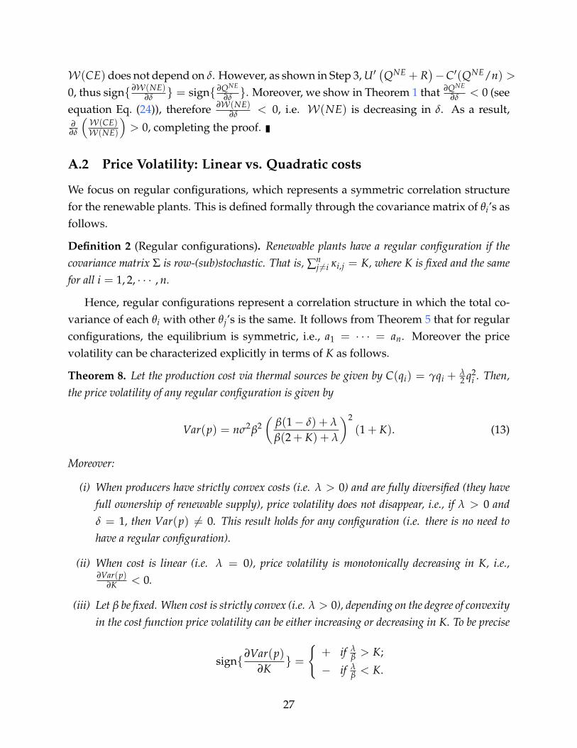
W(CE) does not depend on δ. However, as shown in Step 3, U′(QNE + R
)−C′(QNE/n) >
0, thus sign{ ∂W(NE)∂δ } = sign{ ∂QNE
∂δ }. Moreover, we show in Theorem 1 that ∂QNE
∂δ < 0 (seeequation Eq. (24)), therefore ∂W(NE)
∂δ < 0, i.e. W(NE) is decreasing in δ. As a result,∂∂δ
(W(CE)W(NE)
)> 0, completing the proof.
A.2 Price Volatility: Linear vs. Quadratic costs
We focus on regular configurations, which represents a symmetric correlation structurefor the renewable plants. This is defined formally through the covariance matrix of θi’s asfollows.
Definition 2 (Regular configurations). Renewable plants have a regular configuration if thecovariance matrix Σ is row-(sub)stochastic. That is, ∑n
j 6=i κi,j = K, where K is fixed and the samefor all i = 1, 2, · · · , n.
Hence, regular configurations represent a correlation structure in which the total co-variance of each θi with other θj’s is the same. It follows from Theorem 5 that for regularconfigurations, the equilibrium is symmetric, i.e., a1 = · · · = an. Moreover the pricevolatility can be characterized explicitly in terms of K as follows.
Theorem 8. Let the production cost via thermal sources be given by C(qi) = γqi +λ2 q2
i . Then,the price volatility of any regular configuration is given by
Var(p) = nσ2β2(
β(1− δ) + λ
β(2 + K) + λ
)2
(1 + K). (13)
Moreover:
(i) When producers have strictly convex costs (i.e. λ > 0) and are fully diversified (they havefull ownership of renewable supply), price volatility does not disappear, i.e., if λ > 0 andδ = 1, then Var(p) 6= 0. This result holds for any configuration (i.e. there is no need tohave a regular configuration).
(ii) When cost is linear (i.e. λ = 0), price volatility is monotonically decreasing in K, i.e.,∂Var(p)
∂K < 0.
(iii) Let β be fixed. When cost is strictly convex (i.e. λ > 0), depending on the degree of convexityin the cost function price volatility can be either increasing or decreasing in K. To be precise
sign{∂Var(p)∂K
} ={
+ if λβ > K;
− if λβ < K.
27
This result has two important consequences. First, when cost function is sufficientlyconvex, i.e. λ > 0, in contrast to the linear cost (see Proposition 1), price volatility doesnot disappear when δ = 1. This is simply because when thermal producers are fully di-versified, i.e. δ = 1, and their cost function is convex, i.e. λ > 0, then the total supply(via thermal and renewable sources) of each producer i still depends on θi (this will bemore clear by the following Example). Second, the monotonicity of price volatility in Kdepends on the extent of convexity in the cost function. That is, assuming β is fixed,depending on the extent of convexity in the cost function, price volatility can be eitherincreasing or decreasing in K. In fact, in contrast to the linear cost function, with increas-ing the extent of convexity in the cost function, price volatility can become increasing inK. To see this, suppose the cost function from thermal sources, i.e. C(qi), is sufficientlyconvex in qi, so that production from thermal sources is so expensive. Therefore, eachdiversified thermal producer cuts its production via thermal sources (i.e. qi(θi) becomessmall). As a result, the aggregate production in the economy mostly comes form theaggregate renewable supply. That is, Aggregate production = ∑n
i=1 qi(θ) + ∑ni=1 Ri ≈
∑ni=1 Ri = R + ∑n
i=1 θi, where R is constant. Hence, increasing correlation, i.e. K, increasesVar(∑n
i=1 θi) = 1TΣ1 = nσ2(1 + K), increasing volatility in the aggregate production.Thus, price volatility can increase with increasing K, given λ is sufficiently large.
Proof of Theorem 8. The proof follows similar steps as in the proofs of Theorem 5 andProposition 1. In the first part the analysis is for a general configuration. Next we focuson the regular configurations.General configuration Given that C(qi) = γqi +
λ2 q2
i , producer i’s objective is to choose qi
maximizing
Eθ−i(Πi|Ri) = E{p(qi − q fi + δiRi) + p f
i q fi − γqi −
λ
2q2
i |Ri}
where qj(θj) = bj − ajθj, for all j 6= i, and p = α − β(qi + Ri + ∑j 6=i Rj + ∑j 6=i qj). SinceRi = R/n + θi, for all i = 1, 2, · · · , n, thus, the first order optimality condition (FOC)implies
α− γ− β
(∑j 6=i
E[qj(θj)|Ri] + ∑j 6=i
E[θj|Ri] + θi + R
)− β(−q f
i + δR/n + δθi) = (2β + λ)qi
(14)
Using the projection theorem: E[qj(θj)|Ri] = bj − ajκi,jθi and E[θj|Ri] = κi,jθi.
28
As a result rearranging terms in Eq. (14) gives(α− γ− β
(∑j 6=i
bj + R− q fi + δR/n
))− θiβ
((1 + δ) + ∑
j 6=iκi,j −∑
j 6=iajκi,j
)= ((2β + λ)bi)− θi((2β + λ)ai) (15)
To analyze price volatility we only need to find ai for i = 1, 2, · · · n. Thus, we onlyneed to equate the coefficient of θi in the LHS and RHS of Eq. (15), that implies (note thatβ > 0)
∑j 6=i
κi,jaj +
(2 +
λ
β
)ai = (1 + δ) + ∑
j 6=iκi,j ≡ vi (16)
⇒ Aa = v,
where A ≡ 1σ2 Σ +
(1 + λ
β
)I, and I denotes the identity matrix. Since A is positive define,
it is invertible and thus
a = A−1v
=
(1σ2 Σ + (1 +
λ
β)I)−1
(δ1 +1σ2 Σ1)
=
(1σ2 Σ + (1 +
λ
β)I)−1(
(δ− (1 +λ
β)) I +
1σ2 Σ + (1 +
λ
β) I)
1
= 1 + (δ−(
1 +λ
β
))
((1 +
λ
β
)I +
1σ2 Σ
)−1
1. (17)
As shown in the proof of Proposition 1, Var(p) = (a− 1)TΣ(a− 1), thus
Var(p) = (δ−(
1 +λ
β
))2 1T
((1 +
λ
β
)I +
1σ2 Σ
)−1
Σ((
1 +λ
β
)I +
1σ2 Σ
)−1
1
Thus, when λ > 0 and δ = 1 (in contrast to the linear cost), Var(p) 6= 0.Regular configuration For regular configurations a1 = · · · = an ≡ a. Thus Eq. (16)implies a = β(1+δ+K)
β(K+2)+λ.
Moreover, as shown in the proof of Proposition 1, Var(p) = β2Var (∑ni=1(ai − 1)θi),
thus for regular configurations we have
Var(p) = β2(a− 1)21TΣ1 = nσ2β2(
β(1− δ) + λ
β(2 + K) + λ
)2
(1 + K).
29
The explicit characterization of Var(p) implies that
∂Var(p)∂K
=
(nσ2β2 (β(1− δ) + λ)2
(β(2 + K) + λ)3
)[λ− βK]
completing the proof.
Example (Duopoly with incomplete information and quadratic cost) Let us as-sume each producer i ∈ {1, 2} owns a generator that produces qi units of thermal en-ergy at cost C(qi) = λ
2 q2i (where λ > 0). In this economy thermal producers are also
capable to generate energy from renewable plants. To this end, we assume there aretwo intermittent plants. Let `1 and `2 denote the locations of these plants. Each pro-ducer i privately observes the available renewable energy Ri at local plant li. We assumeRi = R/2 + θi, where R is a constant, and θi is normally distributed with mean zero andvariance σ2, i.e., θi ∼ N (0, σ2). The vector θ = (θ1, θ2) is assumed to be jointly normaland cov(θ1, θ2) = κσ2, where κ ∈ [0, 1]. The scalar κ captures the correlation betweenavailable renewable energy at plants li and lj.16
For ease of exposition we assume p ≡ α− (q1 + q2 + R1 + R2), consequently,17 pro-ducer i’s (ex-post) payoff becomes:
Πi = p(qi + δRi)− λq2
i2
= (α− q1 − q2 − R1 − R2)(qi + δRi)− λq2
i2
.
Solving this case implies
qi(θi) =α− R− δR/2
λ + 3−(
1 + δ + κ
λ + 2 + κ
)θi
Var[p] = 2σ2(
λ + 1− δ
λ + 2 + κ
)2
(1 + κ) (18)
Therefore, with increasing λ, intuitively, production from thermal sources decreases, i.e.∂E[qi(θi)]
∂λ < 0.Furthermore, using Theorem 8, we have
∂Var(p)∂κ
=
(2σ2(λ + 1− δ)2
(λ + 2 + κ)3
)(λ− κ).
Therefore, depending on the extent of convexity in the cost function, price volatility can
16It is worth noting that adding forward contract does not have any effect on the price volatility.17In this simple example we assume β = 1.
30
be decreasing or increasing with respect κ. To be precise:
sign(∂Var(p)
∂κ) = sign(λ− κ)
where as for the linear cost price volatility monotonically decreases in κ (see Lemma 6).
A.3 Degrees of convexity and concavity
This section analyzes the effects of convex cost and concave inverse demand functionson the market price, when thermal producers have a diverse energy portfolio. We show,for a given concave inverse demand function, with increasing extent of convexity in thecost function market price goes up. However, for a given convex cost function, withincreasing extent of concavity in the inverse demand market price goes down. To thisend, we consider two cases as follows. Without loss of generality we assume n = 2.
Concavity analysis of the inverse demand Let the cost function be a given convexfunction (i.e. C′′ ≥ 0), and inverse demand be p = P(Q) = α− βQ2, where β > 0. Thus,the more β is, the more concave the inverse demand P(Q) is. The objective is to show∂p∂β < 0.
The profit of each (diverse) thermal producer is given by
Πi = (qi + δR/2)P(Q + R)− C(qi) = (qi + δR/2)(α− β(Q + R)2)− C(qi)
FOC then gives ∂Πi∂qi
= (α− β(Q + R)2) + (qi + δR/2)(−2β(Q + R))− C′(qi) = 0. Due tosymmetry (at equilibrium) q1 = q2. Thus,
0 = (α− β(Q + R)2) + (Q + δR)(−β(Q + R))− C′(Q/2).
Taking a derivative with respect β implies
[(Q + R)2 + (Q + δR)(Q + R)
]+
∂Q∂β
[3β(Q + R) + β(Q + δR) + 1/2C′′(Q/2)
]= 0.
Thus (note that C′′ ≥ 0),
∂Q∂β
= − (Q + R)2 + (Q + δR)(Q + R)3β(Q + R) + β(Q + δR) + 1/2C′′(Q/2)
< 0.
What is the effect of inverse demand concavity (controlled by β) on the market price p?
31
Since p = α− β(Q + R)2, thus
∂p∂β
= −(Q + R)2 − 2β(Q + R)∂Q∂β
= −(Q + R)2[
1− 2βQ + R + Q + δR
3β(Q + R) + β(Q + δR) + 1/2C′′(Q/2)
]≤ 0,
where the last inequality is correct because [...] ≥ 0 (note that δ ∈ [0, 1] and C′′ ≥ 0).Therefore, with increasing extent of concavity in the inverse demand market price de-creases.Convexity analysis of the cost function Let the inverse demand be concave (and down-ward) (i.e. P′′ ≤ 0 and P′ < 0) and the cost function be C(qi) = γqi +
λ2 q2
i , where γ ≥ 0and λ ≥ 0 . Thus, the more is λ, the more convex is the cost function C(qi). The objectiveis to show ∂p
∂λ > 0.The analysis is inline with the previous case. The profit of each (diverse) thermal
producer is updated by Πi = (qi + δR/2)P(Q + R) − C(qi) = (qi + δR/2)P(Q + R) −(γqi +
λ2 q2
i
). The FOC then gives ∂Πi
∂qi= P(Q + R) + (qi + δR/2)P′(Q + R)− (γ + λqi).
Due to the symmetry (at equilibrium) q1 = q2. Thus,
0 = P(Q + R) + (12)(Q + δR)P′(Q + R)−
(γ + λ
Q2
).
Taking a derivative with respect λ and rearranging terms imply
∂Q∂λ
=Q
3P′(Q + R) + (Q + δR)P′′(Q + R)− λ< 0,
where the last inequality is because the inverse demand in downward and concave (i.e.P′ < 0 and P′′ ≤ 0). Thus, with increasing convexity in the cost function aggregateproduction decreases. As a result, since P is decreasing in Q (i.e. P′ < 0), thus the marketprice increases in λ, completing the proof.
32
B Proofs omitted from main text
B.1 Merit order effect vs. Diversification
Proof of Theorem 1. We present the proof for the duopoly case, extension to n ≥ 2 isstraightforward. With the concave (downward) inverse demand P and the convex cost C,profit of each (diverse) thermal producer is given by
Πi = (qi + δR/2)P(Q + R)− C(qi), (19)
where each conventional generator owns δR/2 units of renewable supply, δ ∈ [0, 1].We first note that
∂p∂R
=
(∂Q∂R
+ 1)
P′(Q + R), (20)
where p ≡ P(Q + R). Since P′ is downward (i.e. P′ < 0), thus to show ∂p∂R ≤ 0, we next
prove that ∂Q∂R + 1 ≥ 0.
FOC implies
0 =∂Πi
∂qi= P(Q + R) + (qi + δR/2)P′(Q + R)− C′(qi)
By symmetry q1 = q2, thus the above equation is equivalent to
0 =∂Πi
∂qi= P(Q + R) + (
12)(Q + δR)P′(Q + R)− C′(Q/2) (21)
Taking derivative from Eq. (21) with respect to R implies
0 =
(1 +
∂Q∂R
)P′(Q + R) + (
12)
(1 +
∂Q∂R
)(Q + δR)P′′(Q + R)
+ (12)
(δ +
∂Q∂R
)P′(Q + R)− (
12)
(∂Q∂R
)C′′(
Q2
)Rearranging terms yields
0 =
[3P′(Q + R) + (Q + δR)P′′(Q + R)− C′′
(Q2
)]∂Q∂R
+[(2 + δ)P′(Q + R) + (Q + δR)P′′(Q + R)
]
33
Consequently,
∂Q∂R
= − (2 + δ)P′(Q + R) + (Q + δR)P′′(Q + R)
3P′(Q + R) + (Q + δR)P′′(Q + R)− C′′(
Q2
) (22)
Recall that the cost function is convex, thus C′′ ≥ 0. As a result, with linear cost, C′′ = 0,since P′ < 0 and P′′ < 0, thus Eq. (22) implies
−1 ≤ ∂Q∂R
< 0 ⇒ 1 +∂Q∂R≥ 0, and with δ = 1, − 1 =
∂Q∂R
. (23)
Thus, using Eq. (20), we obtain ∂p∂R ≤ 0. Moreover, when all renewable supply generates
profits for only conventional power generators (i.e. δ = 1), ∂p∂R = 0, neutralizing the MoE.
However, with strictly convex cost (i.e. C′′ > 0), for δ ∈ [0, 1]:
0 >∂Q∂R
= − (2 + δ)P′(Q + R) + (Q + δR)P′′(Q + R)
3P′(Q + R) + (Q + δR)P′′(Q + R)− C′′(
Q2
)> − (2 + δ)P′(Q + R) + (Q + δR)P′′(Q + R)
3P′(Q + R) + (Q + δR)P′′(Q + R)
≥ −1.
As a result, ∂Q∂R + 1 > 0, consequently, using Eq. (20), ∂p
∂R < 0 for all δ ∈ [0, 1]. Therefore,full neutralization may not be obtained with strictly convex cost functions.
To wrap up the proof we next show ∂p∂δ > 0, diversification amplifies the prices. Since
∂p∂δ
=
(∂Q∂δ
)P′(Q + R)︸ ︷︷ ︸
<0
to prove the claim is then sufficient to show ∂Q∂δ < 0. Taking a derivative from Eq. (21)
with respect to δ implies
0 =
(∂Q∂δ
)P′(Q + R) + (
12)
(∂Q∂δ
)(Q + δR)P′′(Q + R) + (
12)
(R +
∂Q∂δ
)P′(Q + R)
− (12)
(∂Q∂δ
)C′′(
Q2
)
34
Rearranging terms gives
0 =
[3P′(Q + R) + (Q + δR)P′′(Q + R)− C′′
(Q2
)]∂Q∂δ
+ RP′(Q + R)
Therefore,
∂Q∂δ
= − RP′(Q + R)
3P′(Q + R) + (Q + δR)P′′(Q + R)− C′′(
Q2
) < 0, (24)
completing the proof of the first part.To prove the second part we note that since P′ 6= 0, thus ∂p
∂R =(
∂Q∂R + 1
)P′(Q +
R) = 0 if and only if ∂Q∂R = −1. Therefore, when δ → 1, using Eq. (22), we obtain
∂Q∂R = −1 if and only if C′′ = 0. Thus, under any condition ensuring a unique interiorequilibrium, neutralization result prevails when (i) thermal producers are diversified, (ii)cost of production (via thermal sources) is either linear or constant, i.e. C′′ = 0.
It is worthy to note that, inspired by the standard Cournot model (see Ch 4 of Vives[1999] and Kolstad and Mathiesen [1987]), a unique equilibrium is ensured in our model
if: (i) C′′ − P′(Q + R) > 0, (ii) P′(Q+R)+(qi+δ R2 )P′′(Q+R)
C′′−P′(Q+R) < 1n , where n denotes the number
of thermal generators.
C Derivations of the reduced-from models
Proof of Theorem 2. Since Πi = (α− β(∑i qi +R))(qi + δR/n)−γqi, thus FOC impliesα − β(qi + ∑j 6=i qj + R) − β(qi + δR/n) − γ = 0, for all i = 1, 2, · · · , n. Taking a sumover all i implies n(α − γ) − nβ(Q + R) − β(Q + δR) = 0. Hence, at the equilibrium,Q = n(α−γ)−β(δR+nR)
β(n+1) . By symmetry, qi = Q/n = α−γ−β(δR/n+R)β(n+1) , for all i = 1, 2, · · · , n.
Further, plugging Q into p = α− β(Q + R) implies p = α+β(−R+δR)+nγn+1 , as desired.
Proof of Theorem 4. To have a better understanding of the proof steps we first considerthe duopoly case. The oligopoly case is more involved but it follows similar steps.
Consider the duopoly case, i.e. n = 2. By adding forward contract to the previous casethe profit of each generator becomes Πi(q1, q2) = (α− β(q1 + q2 + R))(qi − q f
i + δR/2) +q f
i p fi − γqi. In this case, the economy has two dates, t = 1, 2: generators sign forward con-
tract at t = 1 and the market clearing price p = α− β(∑ni=1 qi + R) is characterized at the
final date t = 2. The solution strategy is to work backward. Thus, given (q f1 , p f
1 , q f2 , p f
2),
35
FOC implies
0 =∂Πi
∂qi= α− γ− β(q1 + q2 + R)− β(qi − q f
i + δR/2). (25)
Summing over i ∈ {1, 2} and rearranging terms imply Q = 13β
(2α− 2βR− β(−Q f + δR)− 2γ
).
Plugging Q into Eq. (25) and some alegra yield
qi =1
3β
(α− γ− β(Q f − 3q f
i + R + δR/2))
.
Now, given the optimal supply at the final date, we next characterize the optimal forwardcontract for each generator. Note that assuming no possibility for arbitrage implies att = 1 the forward quantity q f
i is signed at the market price, i.e. p fi = p. Thus, optimal
q fi maximizes p(qi + δR/2)− γqi, where p = α− β(q1 + q2 + R). Since ∂p
∂q fi
= −β/3 and
∂qi
∂q fi
= 2/3, thus FOC gives ∂p
∂q fi
(qi + δR/2)+ p ∂qi
∂q fi
−γ∂qi
∂q fi
= − β3 (qi + δR/2)+ (p−γ)2
3 = 0.
Simplifying this equation after plugging Eq. (25) into it, implies
q f1 = q f
2 =1
5β
(α− γ + β(−R + δR)
).
Plugging q fi into Eq. (25) yields qi =
25β
(α− γ + β(−R− δR/4)
). Finally, market price
becomes p = α− β(q1 + q2 + R) = 15
(α + 4γ + β(−R + δR)
).
We next consider the oligopoly case, i.e. n ≥ 2. Given the profit of producer i, i.e.Πi(qi, q−i) = (α− β(qi + ∑j 6=i qj + R))(qi − q f
i + δR/n) + q fi p f
i − γqi, employing the FOC
implies α− γ− β(
∑j 6=i qj + R− q fi + δR/n
)= 2βqi. Thus, rearranging terms yields
α− γ− β
(2qi + ∑
j 6=iqj + R− q f
i + δR/n
)= 0. (26)
Let Q ≡ ∑nj=1 Qj. Taking a sum over all i from Eq. (26) implies
Q =n(α− γ− βR)− β(−Q f + δR)
(n + 1)β, (27)
where Q f ≡ ∑ni=1 q f
i .
36
Next, from Eq. (26) we obtain
α− β(Q + R)− β(−q fi + δR/n)− γ = βqi.
The LHS of the above equation can be simplified as follows:
LHS = (α− γ)− βR− β(q fi + δR/n)− βQ
=1
n + 1
((n + 1)[(α− γ)− βR− β(−q f
i + δR/n)]− n(α− γ) + nβR + β(−Q f + δR))
=1
n + 1
((α− γ)− β
[Q f − (n + 1)q f
i + R + δR/n])
Therefore, we have
qi =1
(n + 1)β
(α− γ− β
[Q f − (n + 1)q f
i + R + δR/n])
. (28)
Next, we move to the contracting stage.Contracting stage Equipped with the results from the production stage, we next findoptimal forward quantities, i.e. q f
1 , q f2 , · · · , q f
n. Importantly, due to the no arbitrage as-sumption p f
i = p. Thus, producer i’s optimal choice for q fi should maximize(
α− β(Q(q fi , q f−i) + R)
)(qi(q
fi , q f−i) + δR/n)− γqi(q
fi , q f−i).
Thus, the FOC gives
(α− β(Q(q fi , q f−i) + R))
∂qi(qfi , q f−i)
∂q fi
− β∂Q(q f
i , q f−i)
∂q fi
(qi(q
fi , q f−i) + δR/n
)− γ
∂qi(qfi , q f−i)
∂q fi
= 0
(29)
Since∂qi(q
fi ,q f−i)
∂q fi
= nn+1 (see Eq. (28)) and
∂Q(q fi ,q f−i)
∂q fi
= 1n+1 (see Eq. (27)), thus Eq. (29) yeilds
(α− β(Q(q fi , q f−i) + R))
nn + 1
− γn
n + 1− (qi(q
fi , q f−i) + δR/n)
β
n + 1= 0 (30)
multiplying in (n + 1) and rearranging terms give −β(qi(qfi , q f−i) + nQ(q f
i , q f−i)) + n(α−
γ)− β(δR/n + nR) = 0. By symmetry q1(qf1 , q f−1) = q2(q
f2 , q f−2) = · · · = qn(q
fn, q f−n), thus
−β(n2 + 1)qi(qfi , q f−i) + n(α− γ)− β(δR/n + nR) = 0. (31)
37
Moreover, Eq. (28) gives that−β(n2 + 1)qi(qfi , q f−i) = −
n2+1n+1
(α− γ− β
[−q f
i + R + δR/n])
,
note that by symmetry q f1 = q f
2 = · · · = q fn.
Plugging this into Eq. (31) gives
− (n2 + 1)[α− γ− β(−q f
i + R + δR/n)]+ (n2 + n)(α− γ)− (n + 1)β(δR/n + nR) = 0.
(32)
Rearranging terms implies
(n2 + 1)βq fi = (n− 1)(α− γ) + (n2 + 1)β(R + δR/n)− (n + 1)β(δR/n + nR)
= (n− 1)[α− γ + β(−R + δR)].
Thus
q fi =
n− 1(n2 + 1)β
(α− γ + β(−R + δR)
). (33)
Thus, we finally find qi by plugging q fi into Eq. (28). That is
qi =1
(n + 1)β
(α− γ− β(−q f
i + R + δR/n))
=1
(n + 1)β
(α− γ− β
[− n− 1(n2 + 1)β
(α− γ + β(−R + δR)
)+ R + δR/n
])=
n(n2 + 1)β
(α + β
(−R− δR
n2
)− γ
).
With the characterization of qi, i = 1, 2 · · · , n, the proof is complete.
D Correlated shocks and incomplete information with
endogenous forward contract
D.1 Equilibrium characterization
Proof of Theorem 5. It is useful to construct the equilibrium sequentially and work back-ward. We start by deriving the optimal behavior at the production stage, for any given setof forward contract level (q f
i , p fi )i=1,··· ,n that summarizes the behavior at the production
stage. Next, we analyze the optimal behavior at the contracting stage.
38
Production stage For a given profile of contracting profile ((q f1 , p f
1), · · · , (q fn, p f
n)), theproduction stage is a game with imperfect competition in the class of normal linear-quadratic games with correlated types, once a generator information Ri is establishedas the type. A strategy qi is a mapping from the information set into the real space:qi : R → R+ for a given individual contracting choice (q f
i , p fi ). We focus on linear equi-
libria at the production stage throughout, that is for each generator i = 1, · · · , n, thereexists ai and bi such that qi(Ri) = bi − aiθi. Optimality for generator i at the productionstage requires that strategy qi maximizes the conditional expected utility, taking all othergenerators strategies q−i as given. Furthermore, applying the projection theorem,18 withthe linear information structure conditional expectations E(θj|θi) are linear in θi, for alli, j.
Producer i chooses qi to maximize
Eθ−i(Πi|Ri) = E{p(qi − q fi + δiRi) + p f
i q fi − γqi|Ri}
where qj(θj) = bj − ajθj, for all j 6= i, and p = α− β(qi + Ri + ∑j 6=i Rj + ∑j 6=i qj). Recallthat Ri = R/n + θi, for all i = 1, 2, · · · , n, thus, the first order conditions (FOC) gives
α− γ− β
(∑j 6=i
E[qj(θj)|Ri] + ∑j 6=i
E[θj|Ri] + θi + R
)− β(−q f
i + δR/n + δθi) = 2βqi (34)
Using the projection theorem:
E[qj(θj)|Ri] = E[qj(θj)|θi] = bj − aj Cov(θi, θj) σ−2 θi = bj − ajκi,jθi
E[θj|Ri] = E[θj|θi] = Cov(θi, θj) σ−2 θi = κi,jθi. (35)
Plugging Eq. (35) into Eq. (34) and rearranging terms gives(α− γ− β
(∑j 6=i
bj + R− q fi + δR/n
))− θiβ
((1 + δ) + ∑
j 6=iκi,j −∑
j 6=iajκi,j
)= (2βbi)− θi(2βai) (36)
18Let θ and ν be random variables such that (θ, ν) ∼ N (µ, Σ) such that:
µ ≡(
µθ
µν
)Σ ≡
(Σθ,θ Σθ,νΣν,θ Σν,ν
)are expectations and variance-covariance matrix, then the conditional density of θ given ν is normal withconditional mean µθ + Σθ,νΣ−1
ν,ν(ν− µν) and variance-covariance matrix Σθ,θ − Σθ,νΣ−1ν,νΣν,θ , provided that
Σν,ν is non-singular, DeGroot [1970].
39
Next, to find ai, we only need to equate the coefficient of θi in the LHS and RHS ofEq. (36), that implies (note that β > 0)
∑j 6=i
κi,jaj + 2ai = (1 + δ) + ∑j 6=i
κi,j ≡ vi (37)
⇒ Aa = v,
where A ≡ 1σ2 Σ + I, and I denotes the identity matrix. Since A is positive define, it is
invertible and thus
a = A−1v, (38)
that is a1
a2...
an
=
2 κ1,2 · · · κ1,n
κ2,1 2 · · · κ2,n...
... . . . ...κn,1 κn,2 · · · 2
−1
1 + δ + ∑j 6=1 κ1,j
1 + δ + ∑j 6=2 κ2,j...
1 + δ + ∑j 6=n κn,j
.
Thus,
a =
(I +
1σ2 Σ
)−1(δ1 +
1σ2 Σ1
)=
(I +
1σ2 Σ
)−1 ((δ− 1)1 + 1 +
1σ2 Σ1
)= 1 + (δ− 1)
(I +
1σ2 Σ
)−1
1.
Similarly, we derive bi. Equating the terms that are independent of θi in the LHS and RHSof Eq. (36) implies
α− γ− β
(∑j 6=i
bj + R− q fi + δR/n
)= 2βbi
⇒ α− γ− β
(2bi + ∑
j 6=ibj + R− q f
i + δR/n
)= 0. (39)
Let b ≡ ∑nj=1 bj. Taking a sum over all i from Eq. (39) gives
b =nα− nγ− nβR− β(−Q f + δR)
(n + 1)β(40)
40
where Q f ≡ ∑ni=1 q f
i . In addition, from Eq. (39) we have
α− βb− βR− β(−q fi + δR/n)− γ = βbi.
The LHS of the above equation can be simplified as follows:
LHS = (α− γ)− βR− β(q fi + δR/n)− βb
=1
n + 1
((n + 1)[(α− γ)− βR− β(−q f
i + δR/n)]− n(α− γ) + nβR + β(−Q f + δR))
=1
n + 1
((α− γ)− βR− β
[(−(n + 1)q f
i +n + 1
nδR)+ Q f − δR
])=
1n + 1
((α− γ)− β
[Q f − (n + 1)q f
i + R + δR/n])
Therefore, we finally have
bi =1
(n + 1)β
(α− γ− β
[Q f − (n + 1)q f
i + R + δR/n])
. (41)
Equations Eq. (41) and Eq. (38) summarize the unique linear equilibrium in the pro-duction stage.Stage 1: Contracting stage Equipped with the results from the production stage, we nextevaluate the amount of optimal forward contract q f
i for each generator i = 1, 2, · · · , n,at the average market price p f
i = Eθ[p] (due to the no arbitrage assumption). This isachieved by computing expected payoff of each generator. Thus, generator i’s optimalchoice for q f
i should maximize
Eθ
[(α− β(qi(q
fi , q f−i) + Ri + ∑
j 6=iRj + ∑
j 6=iqj(q
fj , q f−j))
)(qi(q
fi , q f−i) + δRi)− γqi(q
fi , q f−i)
].
The optimal choice in the production stage is linear in the observed information and is inthe form of qi(θi) = bi − aiθi. Characterization of ai and bi (see Eq. (41) and Eq. (38)) gives
∂qi(qfi , q f−i)
∂q fi
=∂bi(q
fi , q f−i)
∂q fi
.
By the above equality and the fact that E[θi] = 0 and E[Ri] = R/n, it is sufficient to findq f
i maximizing
(α− β(b(q fi , q f−i) + R))(bi(q
fi , q f−i) + δR/n)− γbi(q
fi , q f−i).
41
The FOC gives
(α− β(b(q fi , q f−i) + R))
∂bi(qfi , q f−i)
∂q fi
− β∂b(q f
i , q f−i)
∂q fi
(bi(q
fi , q f−i) + δR/n
)− γ
∂bi(qfi , q f−i)
∂q fi
= 0
(42)
Since∂bi(q
fi ,q f−i)
∂q fi
= nn+1 (see Eq. (41)) and
∂b(q fi ,q f−i)
∂q fi
= 1n+1 (see Eq. (40)), thus Eq. (42) gives
(α− β(b(q fi , q f−i) + R))
nn + 1
− γn
n + 1− (bi(q
fi , q f−i) + δR/n)
β
n + 1= 0. (43)
Multiplying Eq. (43) in (n + 1) and rearranging terms yield
−β(bi + nb(q fi , q f−i)) + n(α− γ)− β(δR/n + nR) = 0.
By symmetry b1(qf1 , q f−1) = b2(q
f2 , q f−2) = · · · = bn(q
fn, q f−n), thus
−β(n2 + 1)bi(qfi , q f−i) + n(α− γ)− β(δR/n + nR) = 0. (44)
Further, Eq. (41) implies that (note that by symmetry q f1 = q f
2 = · · · = q fn)
−β(n2 + 1)bi(qfi , q f−i) = −
n2 + 1n + 1
(α− γ− β
[−q f
i + R + δR/n])
Plugging this into Eq. (44) gives
− (n2 + 1)[α− γ− β(−q f
i + R + δR/n)]+
(n2 + n)(α− γ)− (n + 1)β(δR/n + nR) = 0. (45)
Rearranging terms implies
(n2 + 1)βq fi = (n− 1)(α− γ) + (n2 + 1)β(R + δR/n)− (n + 1)β(δR/n + nR)
= (n− 1)(α− γ) + β((n2 + 1)R− (n2 + n)R + [(n2 + 1)− (n + 1)]δR/n)
= (n− 1)(α− γ) + β(−(n− 1)R + (n− 1)δR)
= (n− 1)[α− γ + β(−R + δR)].
42
Thus
q fi =
n− 1(n2 + 1)β
(α− γ + β(−R + δR)
). (46)
Finally, we next find bi. Plugging q fi into Eq. (41) gives
bi =1
(n + 1)β
(α− γ− β(−q f
i + R + δR/n))
=1
(n + 1)β
(α− γ− β
[− n− 1(n2 + 1)β
(α− γ + β(−R + δR)
)+ R + δR/n
])=
1(n + 1)β
(α− γ−
[−(n− 1)[α− γ + β(−R + δR)] + (n2 + 1)β(R + δR/n)
n2 + 1
])
=1
(n + 1)β
(n2 + n)(α− γ) + β(−(n2 + n)R− n2+n
n2 δR)
n2 + 1
=
n(n2 + 1)β
(α + β
(−R− δR
n2
)− γ
).
With the characterization of bi, i = 1, 2 · · · , n, the proof is complete.
E Derivations of price volatility and welfare/profit
E.1 Price volatility
Proof of Proposition 1 and Lemma 6. As shown in Proposition 5 the optimal productionstrategy is in form of qi(Ri) = bi − aiθi, where bi and ai are scalars. Thus
Var(p) = Var
(α− β
(n
∑i=1
(bi − aiθi) +n
∑i=1
(R/n + θi)
))
= β2Var
(n
∑i=1
(ai − 1)θi
)= β2
(aTΣa− 2aTΣ1 + 1TΣ1
)= β2(a− 1)TΣ(a− 1)
= β2(δ− 1)2 1T(
I +1σ2 Σ
)−1
Σ(
I +1σ2 Σ
)−1
1
= β2(δ− 1)2 bTΣb,
43
where b ≡(
I + 1σ2 Σ)−1
1.We next derive price volatility when Definition 2 holds. First note that for regular
configurations, we have vi = 1+ δ+∑j 6=i κi,j = 1+ δ+K, for all i = 1, 2, · · · , n. Therefore,due to Eq. (37), the optimal ai satisfies
2ai + ∑j 6=i
ajκi,j = vi = 1 + δ + K.
Thus, by symmetry, we have a1 = · · · = an = 1+δ+K2+K . Consequently,
Var(p) = β2(
1− 1 + δ + K2 + K
)2
1TΣ1 = nσ2β2(
1− δ
2 + K
)2
(1 + K),
completing the proof.
Proof of Proposition 2. Since the decay factor ζ ∈ (0 1), thus
Kcycle = 2(
ζ + ζ2 + · · ·+ ζn−1
2
)= 2ζ
(1− ζ
n−12
1− ζ
)≤ (n− 1)ζ = Kcomplete
Moreover, by the characterization of price volatility in Lemma 6, it is clear that ∂Var(p)∂K ≤ 0.
Thus, price volatility is in decreasing the decay factor because
∂Var(p)∂ζ
=∂Var(p)
∂K∂K∂ζ︸︷︷︸≥0
≤ 0.
This implies that price volatility in the complete model is less than the cycle model, com-pleting the proof. Note that since κi,j ∈ {0, κ}, for any i 6= j, thus given the definition
of regular structures, for any regular configuration with n renewable plants, K(n)cycle <
K(n)regular < K(n)
complete.
E.2 Welfare/Profit analysis
Before proving Theorem 3, we present two intuitive results about the impact of R and δ
on each thermal producer’s profit. We show diversified energy portfolios are always ben-eficial for thermal producers. However, the profit consequences of increasing renewablesfor diversified thermal producers (i.e. δ > 0) crucially depends on δ. That is, dependingon the extent of δ, increasing renewable supply can be beneficial or detrimental for ther-
44
mal producers. In fact, our model suggests there exists a unique threshold δ∗ for whichwhen thermal producers have a low share from renewable outcome (i.e. δ < δ∗) theirbenefit decreases with increasing renewable supply, but when their share is sufficientlyhigh (i.e. δ > δ∗), increasing renewable supply is actually beneficial for them.
Proposition 3. The payoff of each non-diversified thermal producer monotonically decreases withincreasing renewable supply on the grid, i.e. ∂Πi
∂R < 0 if δ = 0. However, the payoff of each thermalproducer always arises via diversification, i.e. ∂Πi
∂δ > 0.
Proof of Proposition 3. Due to Theorem 2, ∂p∂δ = βR
n+1 > 0, and ∂qi∂δ = −βR/n
(n+1)βthus ∂qi
∂δ + Rn =
Rn (1−
1n+1) > 0. Moreover,
∂Πi
∂δ=
∂p∂δ︸︷︷︸≥0
(qi +
δRn
)+ p
(∂qi
∂δ+
Rn
)︸ ︷︷ ︸
≥0
−γ∂qi
∂δ︸ ︷︷ ︸≥0
≥ 0.
Next, assume δ = 0. Thus, ∂p∂R = −β
n+1 < 0, and ∂qi∂R = −1
(n+1) < 0. Moreover,
∂Πi
∂R=
∂p∂R
qi + p∂qi
∂R− γ
∂qi
∂R
=−β
n + 1qi + (p− γ)
−1n + 1
< 0,
where the last inequality holds because p− γ > 0.
Proposition 4. There exists a unique δ∗ ∈ (0, 1) such that if δ < δ∗ then with increasingrenewable supply the profit of each diversified thermal producer decreases, i.e. ∂Πi
∂R < 0. However,if δ > δ∗ then each diversified thermal producer will be better off with increasing renewable supply,i.e. ∂Πi
∂R > 0.
Proof of Propostion 4. Due to symmetry, the profit of each thermal producer at the equi-librium can be written as Πi = (qi + δR/n)p − γqi = 1
n [(Q + δR)p− γQ], recall thatQ = ∑n
i=1 qi = nqi (at the equilibrium). Further, due to Theorem 2, p = 1(n+1)(α + β(−R +
δR) + nγ) and Q = n(n+1)β
(α− γ− β(R + δR/n)). Plugging p and Q into the profit of the
45
thermal producer i gives
Πi =1n[(Q + δR)p− γQ]
=1
βn(n + 1)
[1
n + 1
(α + β(−R + δR) + nγ
)(n(α− γ)− β(nR + δR) + β(n + 1)δR
)
− γn(
α− γ− β(R + δR/n))]
Let us define Λ ≡ [...] (note that the roots of ∂Πi∂R and ∂Λ
∂R are equivalent). Thus,
∂Λ∂R
=β(δ− 1)
n + 1
(n(α− γ)− β(nR + δR) + β(n + 1)δR
)+−β(δ + n) + (n + 1)δβ
n + 1
(α + β(−R + δR) + nγ
)+ γnβ
(1 +
δ
n
)≡ f (δ).
It is easy to see that f (δ) is quadratic in δ, thus it looks like f (δ) = xδ2 + yδ+ z (where x, y,and z are all independent of δ). First note that x = 2β2Rn
n+1 > 0, thus f (δ) is convex. Nextwe show f (δ) has a unique zero lying between zero and one. To achieve this we showf (0) < 0 and f (1) > 0 (see the following Figure) since f (δ) is continuous and quadraticthus has unique zero in (0, 1).
f (0) = −β
(n(α− γ)− βnR
n + 1
)− nβ
n + 1(α− βR + nγ) + γnβ
=−2nβ
n + 1(α− γ− βR)
< 0
where the last inequality holds since α− γ− βR > 0.
f (1) = γnβ
(1 +
1n
)> 0.
Since f (1) > 0 and f (0) < 0, thus there exists a unique δ∗ ∈ (0, 1) for which f (δ∗) = 0.As a result, ∂Πi
∂R |δ=δ∗ = 0, and consequently, ∂Πi∂R |δ<δ∗ < 0 and ∂Πi
∂R |δ>δ∗ > 0, completing
46
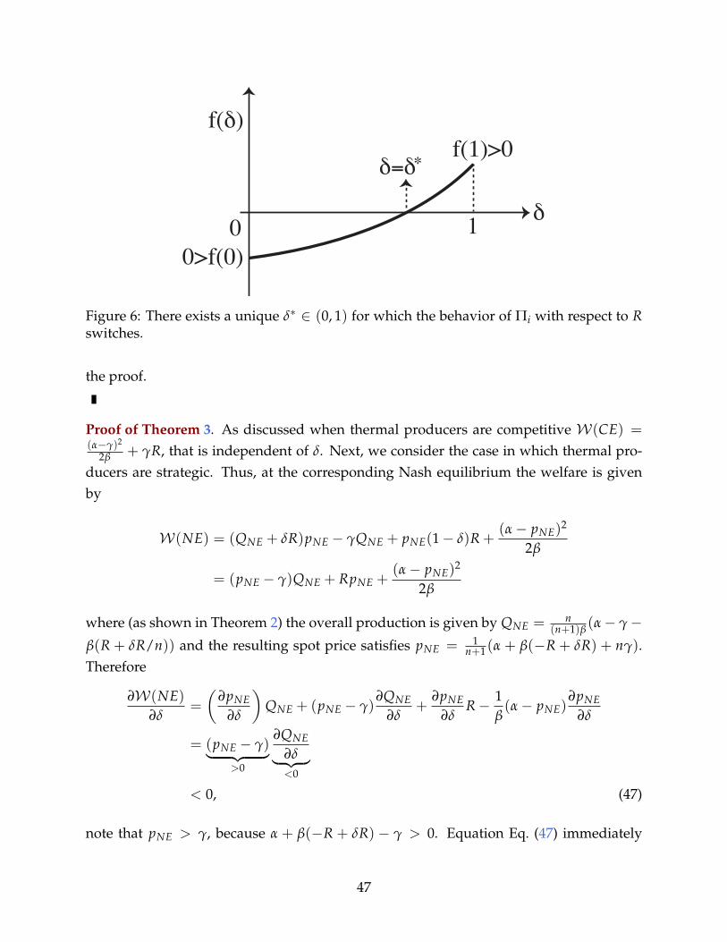
1
δ=δ∗
δ0
f(δ)
f(1)>0
0>f(0)
Figure 6: There exists a unique δ∗ ∈ (0, 1) for which the behavior of Πi with respect to Rswitches.
the proof.
Proof of Theorem 3. As discussed when thermal producers are competitive W(CE) =(α−γ)2
2β + γR, that is independent of δ. Next, we consider the case in which thermal pro-ducers are strategic. Thus, at the corresponding Nash equilibrium the welfare is givenby
W(NE) = (QNE + δR)pNE − γQNE + pNE(1− δ)R +(α− pNE)
2
2β
= (pNE − γ)QNE + RpNE +(α− pNE)
2
2β
where (as shown in Theorem 2) the overall production is given by QNE = n(n+1)β
(α− γ−β(R + δR/n)) and the resulting spot price satisfies pNE = 1
n+1(α + β(−R + δR) + nγ).Therefore
∂W(NE)∂δ
=
(∂pNE
∂δ
)QNE + (pNE − γ)
∂QNE
∂δ+
∂pNE
∂δR− 1
β(α− pNE)
∂pNE
∂δ
= (pNE − γ)︸ ︷︷ ︸>0
∂QNE
∂δ︸ ︷︷ ︸<0
< 0, (47)
note that pNE > γ, because α + β(−R + δR) − γ > 0. Equation Eq. (47) immediately
47
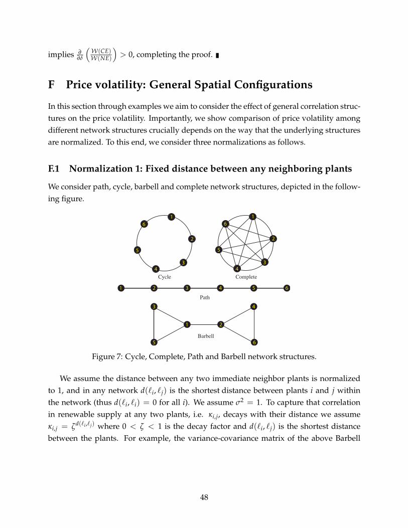
implies ∂∂δ
(W(CE)W(NE)
)> 0, completing the proof.
F Price volatility: General Spatial Configurations
In this section through examples we aim to consider the effect of general correlation struc-tures on the price volatility. Importantly, we show comparison of price volatility amongdifferent network structures crucially depends on the way that the underlying structuresare normalized. To this end, we consider three normalizations as follows.
F.1 Normalization 1: Fixed distance between any neighboring plants
We consider path, cycle, barbell and complete network structures, depicted in the follow-ing figure.
1
2
3
6
1
2
3
6
4
5
4
5
1 2 3 4 5 6
3
1
5
2
4
6
Barbell
Path
Cycle Complete
Figure 7: Cycle, Complete, Path and Barbell network structures.
We assume the distance between any two immediate neighbor plants is normalizedto 1, and in any network d(`i, `j) is the shortest distance between plants i and j withinthe network (thus d(`i, `i) = 0 for all i). We assume σ2 = 1. To capture that correlationin renewable supply at any two plants, i.e. κi,j, decays with their distance we assumeκi,j = ζd(`i,`j) where 0 < ζ < 1 is the decay factor and d(`i, `j) is the shortest distancebetween the plants. For example, the variance-covariance matrix of the above Barbell
48
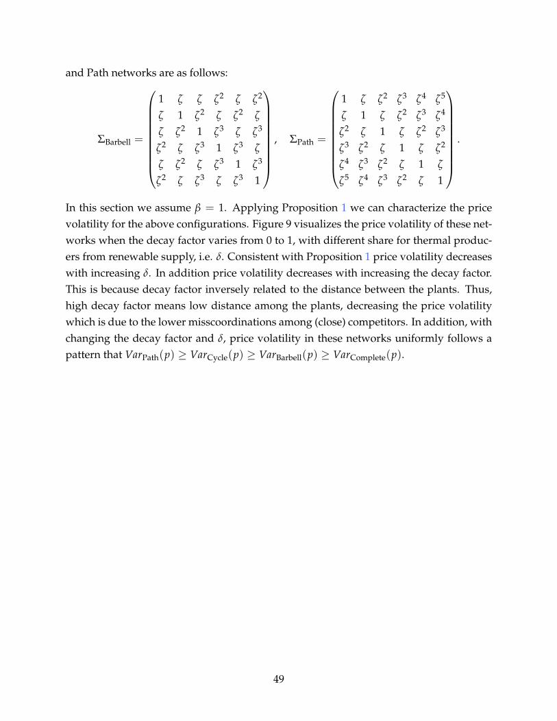
and Path networks are as follows:
ΣBarbell =
1 ζ ζ ζ2 ζ ζ2
ζ 1 ζ2 ζ ζ2 ζ
ζ ζ2 1 ζ3 ζ ζ3
ζ2 ζ ζ3 1 ζ3 ζ
ζ ζ2 ζ ζ3 1 ζ3
ζ2 ζ ζ3 ζ ζ3 1
, ΣPath =
1 ζ ζ2 ζ3 ζ4 ζ5
ζ 1 ζ ζ2 ζ3 ζ4
ζ2 ζ 1 ζ ζ2 ζ3
ζ3 ζ2 ζ 1 ζ ζ2
ζ4 ζ3 ζ2 ζ 1 ζ
ζ5 ζ4 ζ3 ζ2 ζ 1
.
In this section we assume β = 1. Applying Proposition 1 we can characterize the pricevolatility for the above configurations. Figure 9 visualizes the price volatility of these net-works when the decay factor varies from 0 to 1, with different share for thermal produc-ers from renewable supply, i.e. δ. Consistent with Proposition 1 price volatility decreaseswith increasing δ. In addition price volatility decreases with increasing the decay factor.This is because decay factor inversely related to the distance between the plants. Thus,high decay factor means low distance among the plants, decreasing the price volatilitywhich is due to the lower misscoordinations among (close) competitors. In addition, withchanging the decay factor and δ, price volatility in these networks uniformly follows apattern that VarPath(p) ≥ VarCycle(p) ≥ VarBarbell(p) ≥ VarComplete(p).
49
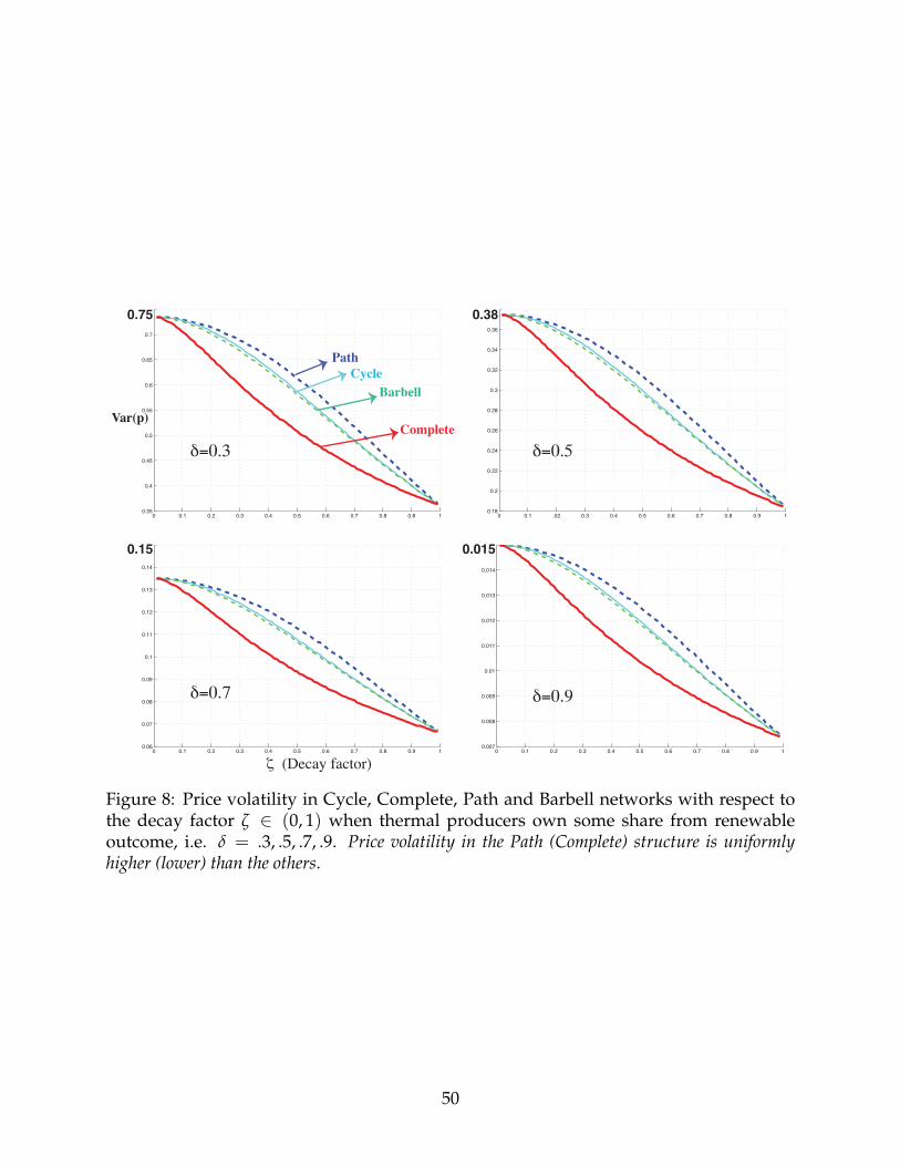
0 0.1 0.2 0.3 0.4 0.5 0.6 0.7 0.8 0.8 10.35
0.4
0.45
0.5
0.55
0.6
0.65
0.7
0.75
0 0.1 .02 0.3 0.4 0.5 0.6 0.7 0.8 0.9 10.18
0.2
0.22
0.24
0.26
0.28
0.3
0.32
0.34
0.36
0.38
0 0.1 0.2 0.3 0.4 0.5 0.6 0.7 0.8 0.9 10.06
0.07
0.08
0.09
0.1
0.11
0.12
0.13
0.14
0.15
0 0.1 0.2 0.3 0.4 0.5 0.6 0.7 0.8 0.9 10.007
0.008
0.009
0.01
0.011
0.012
0.013
0.014
0.015
Path
Cycle
Barbell
Complete
δ=0.3
δ=0.9δ=0.7
δ=0.5
Var(p)
ζ (Decay factor)
Figure 8: Price volatility in Cycle, Complete, Path and Barbell networks with respect tothe decay factor ζ ∈ (0, 1) when thermal producers own some share from renewableoutcome, i.e. δ = .3, .5, .7, .9. Price volatility in the Path (Complete) structure is uniformlyhigher (lower) than the others.
50
F.2 Normalization 2: The same distance for the farthest plants
For this normalization we compare Path and Barbell structures, given that the distancefor their farthest plants is the same. In the Path network the correlation between anytwo “neighboring” plants is ζ, where ζ ∈ (0, 1) is the decay factor. However, the Barbellnetwork consists of two cliques located far from each other. In each clique the correlationbetween any two neighbor plants is ζ. But, since by this normalization, in the Path andBarbell networks the distance between the two farthest plants should be the same, thusthe correlation between the two farthest plants in these networks is ζmaximum distance =
ζ2n−1 (see Figure 10).
Barbell
Path
1
1
2n2 3
n
n+1
2n
1 unit
2n-3 units
Figure 9: Path and Barbell networks. The same distance for the farthest plants.
Now, suppose the decay factor changes from zero to one. Then, as shown in Figures 11and 12, in contrast to the previous case, price volatility with this normalization does notchange uniformly in these network structures. In fact, when decay factor is small (i.e. lowcorrelation in renewable supply for neighboring plants) price volatility in Path is higherthan Barbel structures. But, when decay factor is sufficiently high (i.e. high correlationin renewable supply for neighboring plants) then price volatility in the Path structure islower than the Barbell.
51
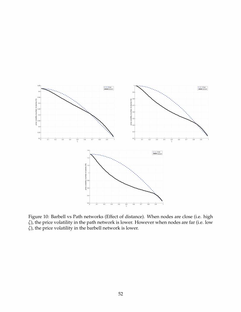
0 0.1 0.2 0.3 0.4 0.5 0.6 0.7 0.8 0.9 10.2
0.25
0.3
0.35
0.4
0.45
0.5
0.55
0.6
0.65
ζ
price
vo
latilit
y (
nu
mb
er
of p
lan
ts=
10
)
Path
Barbell
0 0.1 0.2 0.3 0.4 0.5 0.6 0.7 0.8 0.9 10.2
0.3
0.4
0.5
0.6
0.7
0.8
0.9
1
ζ
price
vo
latilit
y (
nu
mb
er
of p
lan
ts=
16
)
Path
Barbell
0 0.1 0.2 0.3 0.4 0.5 0.6 0.7 0.8 0.9 10.2
0.4
0.6
0.8
1
1.2
1.4
1.6
ζ
price
vo
latilit
y (
nu
mb
er
of p
lan
ts=
24
)
Path
Barbell
Figure 10: Barbell vs Path networks (Effect of distance). When nodes are close (i.e. highζ), the price volatility in the path network is lower. However when nodes are far (i.e. lowζ), the price volatility in the barbell network is lower.
52
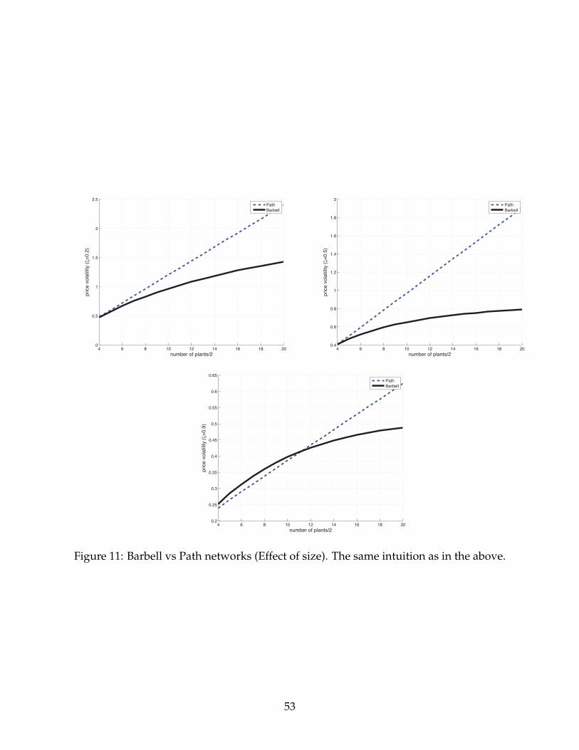
4 6 8 10 12 14 16 18 200
0.5
1
1.5
2
2.5
number of plants/2
price
vo
latilit
y (ζ=
0.2
)
Path
Barbell
4 6 8 10 12 14 16 18 200.4
0.6
0.8
1
1.2
1.4
1.6
1.8
2
number of plants/2
price
vo
latilit
y (ζ=
0.5
)
Path
Barbell
4 6 8 10 12 14 16 18 200.2
0.25
0.3
0.35
0.4
0.45
0.5
0.55
0.6
0.65
number of plants/2
price
vo
latilit
y (ζ=
0.9
)
Path
Barbell
Figure 11: Barbell vs Path networks (Effect of size). The same intuition as in the above.
53
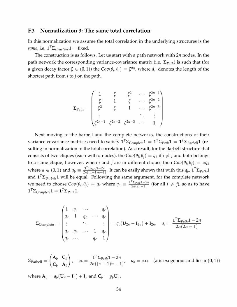
F.3 Normalization 3: The same total correlation
In this normalization we assume the total correlation in the underlying structures is thesame, i.e. 1TΣstructure1 = fixed.
The construction is as follows. Let us start with a path network with 2n nodes. In thepath network the corresponding variance-covariance matrix (i.e. ΣPath) is such that (fora given decay factor ζ ∈ (0, 1)) the Cov(θi, θj) = ζdij , where dij denotes the length of theshortest path from i to j on the path.
ΣPath =
1 ζ ζ2 · · · ζ2n−1
ζ 1 ζ · · · ζ2n−2
ζ2 ζ 1 · · · ζ2n−3
... . . . ...ζ2n−1 ζ2n−2 ζ2n−3 · · · 1
Next moving to the barbell and the complete networks, the constructions of their
variance-covariance matrices need to satisfy 1TΣComplete1 = 1TΣPath1 = 1TΣBarbell1 (re-sulting in normalization in the total correlation). As a result, for the Barbell structure thatconsists of two cliques (each with n nodes), the Cov(θi, θj) = qb if i 6= j and both belongsto a same clique, however, when i and j are in different cliques then Cov(θi, θj) = αqb
where α ∈ (0, 1) and qb ≡ 1TΣPath1−2n2n((α+1)n−1) . It can be easily shown that with this qb, 1TΣPath1
and 1TΣBarbell1 will be equal. Following the same argument, for the complete networkwe need to choose Cov(θi, θj) = qc where qc ≡ 1TΣPath1−2n
2n(2n−1) (for all i 6= j), so as to have1TΣComplete1 = 1TΣPath1.
ΣComplete =
1 qc · · · qc
qc 1 qc · · · qc... . . . ...
qc qc · · · 1 qc
qc · · · qc 1
= qc(U2n − I2n) + I2n, qc =
1TΣPath1− 2n2n(2n− 1)
ΣBarbell =
(Ab Cb
Cb Ab
), qb =
1TΣPath1− 2n2n((α + 1)n− 1)
, yb = αxb (α is exogenous and lies in(0, 1))
where Ab = qb(Un − In) + In and Cb = ybUn.
54
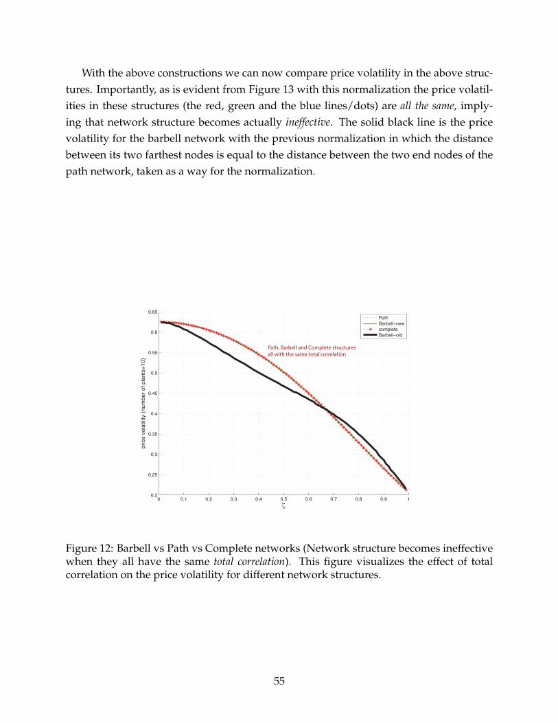
With the above constructions we can now compare price volatility in the above struc-tures. Importantly, as is evident from Figure 13 with this normalization the price volatil-ities in these structures (the red, green and the blue lines/dots) are all the same, imply-ing that network structure becomes actually ineffective. The solid black line is the pricevolatility for the barbell network with the previous normalization in which the distancebetween its two farthest nodes is equal to the distance between the two end nodes of thepath network, taken as a way for the normalization.
0 0.1 0.2 0.3 0.4 0.5 0.6 0.7 0.8 0.9 10.2
0.25
0.3
0.35
0.4
0.45
0.5
0.55
0.6
0.65
ζ
price
volat
ility (
num
ber o
f plan
ts=10
)
PathBarbell−newcompleteBarbell−old
Path, Barbell and Complete structuresall with the same total correlation
Figure 12: Barbell vs Path vs Complete networks (Network structure becomes ineffectivewhen they all have the same total correlation). This figure visualizes the effect of totalcorrelation on the price volatility for different network structures.
55