Competition for fluctuating nutrient

J. Math. Biology (1983) 18:255-280 Journal of

Mathematical Siolosy

�9 Springer-Verlag 1983

Competition for fluctuating nutrient

J. K. Hale *~ and A. S. Somolinos 2

Lefschetz Center for Dynamical Systems, Division of Applied Mathematics, Brown University, Providence, R.I. 02912, USA 2 On leave at Brown University from Universidad de Alcala de Henares, Madrid, Spain

Abstract. A model of the compet i t ion o f n species for a single essential periodically fluctuating nutr ient is considered. Instead of the familiar Michae l i s -Menten kinetics for nutrient uptake, we assume only that the uptake rate functions are positive, increasing and b o u n d e d above. Sufficient condi- t ions for extinction are given. The existence of a nutrient threshold under which the Principle o f Compet i t ive Exclusion holds, is proven. For two species systems the following very general result is proven: All solutions of a r- periodic, dissipative, competi t ive system are either r -per iodic or approach a r -per iodic solution. A complete description o f the geometry o f the Poincar6 opera tor o f the two species system is given.

Key words: Populat ion dyamics - - Ecology - - Periodic solutions

1. Introduction

We consider the following model of the compet i t ion o f n species for a single essential nutrient in limited supply:

n

S ' = D ( S ~ + b e ( t ) - S ) - ~ ( m i / Y i ) f i ( S ) x i i - -1

(1) Xti : mi f i ( S ) x i - Dixi, i = 1, 2 , . . . , n.

Here, S represents the nutrient concentrat ion, and the xi represent the concentrat ion o f the compet ing organism. We assume that the species compete only by lowering the concentra t ion o f the essential nutrient. The compet i t ion takes place in a chemostat . This is an experimental device in which the input flow of nutr ients can be controlled, and an output flow carries away cells, waste and unused nutrients. The constant D > 0 represents the input and output flow, and is referred to as the wash-out rate. We assume the essential nutrient is washed

* This research has been supported in part by the National Science Foundation under contract #MCS 8205355, and in part by the U.S. Army Research Office under contract #DAAG-29-79-C- 0161

256 J .K. Hale and A. S. Somolinos

out in proport ion to its concentration. The D~ > 0 represent the wash-out rate plus the death rate of the corresponding species.

To simulate the seasonal variations of the nutrient, for instance, in the growth of plankton in a lake, we assume that the input of the essential nutrient varies periodically around a mean value S o > 0, with an amplitude b, b < S o; and period r ; that is, according to the law S ~ where e(t) is a prescribed ~--periodic function of mean value zero, and le(t)l ~< 1.

The terms m i f ( S ) are the per capita growth rate fo r the ith species. The constants rni represent the maximum growth rate. The functions f ( S ) are the nutrient uptake rates for the ith species. We will make the following hypothesis concerning these functions: HI : The nutrient uptake rates f ( S ) are continuous increasing functions with continuous bounded derivatives for S positive, f (0 ) = 0 and f (+oo) = 1.

In some parts of our work we will need the stronger hypothesis, H2: The f satisfy H1 and the derivative f l (S) o f f ( S ) is positive.

Hypotheses H 1 and H2 summarize the properties one can reasonably expect of the nutrient uptake rates. I f there is no nutrient there is no uptake, f (0 ) = 0, and there is a saturation effect; that is, the species does not grow appreciably faster when we increase the food supply past a certain point. In particular H1 and H2 are satisfied when the functional response of the species obeys the Holling "non-learning curve". In this case, the kinetics are the same as in the Michaelis- Menten equation for an enzyme catalyzed reaction, that is

f ( S ) = S/ (a i + S) (2)

where a~ is the half-saturation, or Michael is-Menten constant. We will refer to equations with the functions f ( S ) given by (2) as M - M systems. The terms under the summation sign represent the consumption of nutrient

by the n species. The y~ are the yield factors for the ith species feeding on the nutrient. By rescaling x~ to x~/yi, we may assume each yi = 1. Therefore it will be assumed that each y~ = 1.

The advantage of these models with respect to the Lotka-Volterra equations lies in the fact that the parameters of the system can be measured a species at a time before the actual competit ion takes place.

For the case of M - M dynamics one can rewrite Eq. (1) and obtain

' = (rn~ - D~)x~ S a~ +S) = xigdS). Xi

We have x'~ = 0 when S = ,~ = defa~D~/(rn~ - Di). The parameters ,~i are very important. They define the break-even concentra-

tion, i.e. the concentration of nutrient at which the ith species has zero growth rate. In the same spirit, we define for the general system (1),

def m Z ( S ) - D, = g,(S).

The functions g~(S) are increasing and continuously differentiable for S/> 0. They have positive derivatives if H2 is satisfied. We define the breakeven concentration

Xi as gi(Ai)= O.

Competition for fluctuating nutrient 257

We shall use the system (1) also in the alternative form

S' = D ( S ~ + be( t ) - S ) - ~ m ~ f ( S ) x i i = 1

Xti = gi( S ) x i , i = 1, 2 , . . . , n. (l ')

To simplify the mathematical formulation we will extend the definitions of the functions f and gi for negative values of the argument by making f ( S ) an odd function of S. We will prove later that S( t ) > 0 for all t, so that this extension does not affect the biological meaning of the system. It merely simplifies the formulation of some results.

The model described by Eqs. (1) or (1') is a generalization of a model for competi t ion in a chemostat, studied specially by Hsu, Hubbell and Waltman [9] for a constant input, and by Hsu [7] for a periodic input. H. Smith [14] allows a more general form for the periodic input. All papers studying the periodic input case work with two species and the Michael is-Menten dynamics. We refer to the papers of Hsu [7], [8] and H. Smith [14] for a review of the biological background and a survey of the results obtained for M - M systems.

We give now an outline of the organization of the paper, indicating the main results.

In Sect. 2 we study the general case of the competit ion of n species in a fluctuating nutrient. We give sufficient conditions for the extinction of a species due to lack of nutrient or to competit ion from another species. These sufficient conditions generalize, for n dimensions and nutrient uptake functions f~ satisfying H1, the work done by S. B. Hsu [7] for Michael is-Menten systems and two species. In particular, we are able to prove that, in the presence of sufficient nutrient, when all species but one go extinct, the remaining species x~(t) is bounded away from zero, thus improving on the result l imx~( t )>0 , given by Hsu [7].

For M - M systems we prove the existence and give an estimate of a nutrient threshold under which the Principle of Competit ive Exclusion holds, i.e. the species with the smallest break-even concentration h~ wins the competition. This generalizes for fluctuating nutrient inputs the result of Hsu, Hubbell and Waltman [9], that for constant nutrient the species with the smallest h/ always survives.

When the death rates of the individual species are small compared to the wash-out rate, it seems reasonable to make the simplifying assumption D = D1 = . . . . D , . From Sect. 3 on, we will follow Hsu, Hubbell and Waltman [9] and H. Smith [13] and make this assumption. Under this condition, when one makes the change of variables Zo = S + ~ x;, z; = x~, i = 1 . . . . , n, the equation for z0 becomes uncoupled, and it has a globally asymptotically stable z-periodic solution. Insert- ing this periodic solution of the z0 equation into the other equations reduces the system from n + 1 to n-dimensions. In Sect. 3, we prove that the flow of the n + l -d imens iona l system approaches in a certain sense the flow of the n- dimensional system. In particular, if the latter has a globally asymptotically stable periodic solution, then all solutions of the former approach it. Furthermore, the n-dimensional system thus obtained is a "competit ive system" in the sense of M. Hirsch [6].

258 J.K. Hale and A. S. Somolinos

Using the above change of variables the 3-dimensional system describing the competition of two species can be reduced to a two-dimensional competitive system. We prove that the solutions of this system approach only 7-periodic solutions as t--> oo. It turns out that this result is also true for all competitive systems. In section 4 we prove the general result that all periodic, dissipative, two-dimensional systems have trivial dynamics, i.e. all solutions are either r- periodic, or approach a ~--periodic solution. This result generalizes for periodic systems the work of M. Hirsch [5, 6] for autonomous systems.

In the remaining sections we study exclusively the competition of two species. We investigate the resulting two-dimensional, periodic, competitive system using the Poincarb map. It turns out that the Poincar6 map for our system has the same monotonicity properties as the Poincar6 map of the Lotka-Volterra equations with periodic coefficients studied by deMottoni-Schiaffino [11]. This fact allows us to use a wealth of information about the Poincar6 map obtained by the above authors, as long as the properties depend only on the monotony of the map, and not on the particular form of the equation.

In Sect. 5 we investigate the trivial case, when one of the species is absent or dies out. We prove, in our general setting, the conjecture made by H. Smith [14] for M - M systems: When one species dies out the remaining species approaches a unique non-trivial z-periodic solution which is globally asymptotically stable.

In Sect. 6 we study the non-trivial case, where we do not assume a priori the extinction of one species. We prove that all the fixed points of the Poincar6 map lie on a strictly decreasing curve that connects a point in the y-axis with a point in the x-axis. We give sufficient conditions for the existence of non-trivial periodic solutions. Under the assumption that the uptake functions f are analytic, we prove that there is a finite number of periodic solutions, and give a description of the regions of attraction of the Poincar6 map.

We have collected in an appendix some results on dissipative systems, that could be found, in a more general setting, in Hale [3, 4] and Pliss [12, 13]. Here we present the material as it applies to our particular problem. An outline of the proofs is also included to acquaint the non-specialist with the techniques used, and to make the paper self-contained.

2. N-competing species. A nutrient threshold for coexistence

In this section we consider the case of n-competing species. We make some changes of variables that make system (1) more tractable. We prove then that the system obtained preserves the first quadrant and is dissipative. Next we give conditions for the extinction of a species due to lack of nutrient. Under the assumption that there is enough nutrient, we then give conditions for the extinction of a species due to competition. Finally, for M - M systems we prove that the principle of competitive exclusion holds under a certain threshold of nutrient.

2.1. Dissipativeness and its implication

As remarked earlier, we may assume each Yi = 1 in Eq. (1) by replacing xi by xJyi . Let S*(t) be the unique ~--periodic solution of the equation

S' = - D S + D ( S ~ + be(t)) (3)


that is,

Io �9 S*(t) = D (e D ' - 1) -1 e ~ 1 7 6 dr.

It is easy to see that S O- b <~ S * ( t ) ~ S ~ b, and the mean value o f S*(t) is S ~ I f S = S*(t) - z, then z( t) measures the deviation o f S(t) f rom the free running

value o f the nutrient S*(t) in the absence o f all species. The funct ion z( t) satisfies the fol lowing system

n

z ' = - D z + Y. m i x i f ( S * - z) i = 1

(4) Xl = gi(S* - z)xi, i = 1 . . . . , n.

We will say that a system of ordinary differential equat ions )) = f ( t , y) defined in a domain s is dissipative if there exists an R such that all solutions y( t ) with y( t ) ~ 1-2 for all t satisfies l i m , ~ ly(t)l <~ R.

Let x = ( x l , . . . , x,), R+ +l = {(x, z): xi >i O, z ~ 0}.

Lemma 2.1. Suppose (H1) is satisfied. The solutions (x( t), S( t)) o f (1) with data in R+ +l remain in R+ +~ for t >1 0 and the system is dissipative in R "+~ with

lim,_,~ [S*(t) - S(t)] < S o + b

n

lim,_,~ ~ x i<~6-1D(So+b) , 3 = m i n i D i . i - -1

Finally, i f S(O) > O, there is an *7 = ~(S(0), x(0)) such that S( t) > ~q for all t.

Proof It is obvious that solutions (x(t) , S( t )) of (1) with initial da ta (x ~ S ~ in ..+~n+J remain in .,+o"+~ for all t t> 0. For the remainder of the proof, it is convenient to use the variables ( x ( t ) , z ( t ) ) in (4), z ( t ) = S * ( t ) - S ( t ) . I f z ( t ) ~ S ~ then S*(t) - z ( t ) <~ 0 and f ( S * ( t ) - z(t)) <~ O. Thus, z'( t) <~ - D ( S o + b) < 0 if z( t) >1 S O + b. This implies that there is a tt = h(z(O), x(0)) such that z(t) < So + b if t I> tl.

n I f V(x, z ) = ~=~ x ~ - z, then the derivative l;'(x, z) along the solutions o f (4) is

V(x, z) = Z ( m i x i f - Oixi) + D z - 2 m i x i f = D z - Y~ Dixi.

I f 6 = rain D~, then l? ~ - 6 V + (D - 6)z(t). I f D - 6 <~ 0, then V(x( t ) , z(t)) <~ V(x(O), z(0)) exp( -6 t ) . N o w suppose D - 6 > 0. From the preceding paragraph, we know that the solution x(t) , z( t ) satisfies z(t)<~ S ~ for t ~ > t~ = h(x(O), z(0)). Thus, for t/> tl,

V(x( t ) , z(t)) <~ V(x( t , ) , z (h) ) e x p [ - ~ ( t - tl)] + 6 - ' ( D - 6)(S ~ + b)(1 - e-~(~-'~)).

For any e > 0, there is a t2 ~> tl such that V(x( t , ) , z(f i)) e x p [ - 6 ( t - tl)] < s if t/> t2. Thus, for t/> h,

V(x( t ) , z(t)) <- e + ~ - l ( D - 6)(S ~ + b)

xi(t) <- 6 -1D(S~ + b) + e. i = 1

Since e is arbitrary, this shows that l i m , ~ Y x~<~ 6 - x D ( S ~ We have already shown that l im,~ooz(t)<~So+b. This proves the system is dissipative and the estimates stated in the lemma hold.


Since each solution (x(t), z ( t ) )=(x( t ) , S * ( t ) - S ( t ) ) is bounded and f ( 0 ) = O, S~ be(t)> O, the fact that S(0)> 0 implies there is an r /= ~7(S(0), x(0)) such that S ( t ) > 77 > 0 for all t follows immediately from (1). This proves the lemma.

Remark: Note (x(0), S(0)) in R~_ +1 does not imply (x(0), z(0)) in R~_ +1. I f z(0)> 0, then z(t) remains always positive. I f z(0) < 0, then either there exists a t* > 0 such that z ( t )> 0 for all t > t*, or z(t)<~ 0 for all t. In this case, [z(t)l ~ Iz(0)l e x p - D t for all t/> 0 and we claim that each xj - 0 as t ~ oo. I f not, there is an integer k, a constant ~7 > 0 and a sequence tjk ~ oO as j - ~ such that Xk(tjk) > r/. Since Ix~l is bounded, there is an e > 0 such that Xk(t)> r//2 for t c [tjk--e, tjk + e]. Using the equation for z, one sees that this implies z(t)r which is a contradiction.

2.2. Extinction due to lack of nutrient

We say that the ith species becomes extinct if lim,_.oo xi(t) = O. The following result gives conditions for extinction, depending on the nutrient

availability, independently of the competit ion of the other species.

Theorem 2.2. Suppose H1 is satisfied. I f ~o g,(S*) dt <O, i.e. r -t ~of(S*(t)) dt < D J mi, then xi( t )~ 0 exponentially as t ~ +oo.

Remark: I f mi - D~ ~< 0, then the ith species becomes extinct. In fact, m 0 - - D~r = -r ,

mi ~of(S*(t)) d t - D , r + m i [ r - S o f ( S (t)) dt] and the term in the brackets is > 0 since S*(t) bounded implies f ( S* ( t ) ) < 1.

Corollary 2.3. For M - M systems, Ai >i S O is a sufficient condition for extinction of the ith species.

Remark: When all the other species become extinct, we show later that the condition in Theorem 2.2 is also necessary for the extinction of the ith species.

Proof o f Theorem 2.2: From the remark at the end of the last section, without loss of generality, we may assume z(t)>-0 for all t. Since f ( S ) is an increasing function, this implies f ( S * ( t ) - z ( t ) ) < - f ( S * ( t ) ) and, from (4),

d (ln xi)/dt <~ mi( f (S*) - Di/m,).

Let N = N(t ) be such that N~'<~ t < ( N + l ) r and let K be a constant such T

that ~olm~f (S*( t ) ) -Di ld t<-K. Since S* is periodic of period T, we have 1 ~N~ Im~f(S*(t))-Dd dt <~ K. Integrating the above differential inequality from 0

to t, using the periodicity of S* again and the hypothesis, we have

lnxi(t)- lnxi(O)<~ Y. [ m , f ( S * ) - D i ] d t + K < ~ - N e + K k = l

for some e > 0. Thus, In x i ( t )~ -oo as t ~ co and x~(t)-~ 0 exponentially as t ~ ~ .

Proof o f Corollary 2.3: For M - M systems, the condition in Theorem 2.2 becomes ~o ( S * - hi)/(a~ + S*) < 0. Let us first suppose that e(t) ~ 0 and hi >1 S ~ Let I_ = {t 6 [0, ~-]: S * ( t ) - hi <~ 0}, I+ = [0, ~']\I_. I f I+ is empty, the condition is clearly


satisfied. If it is nonempty , we have

f o S*(t) - Ai ai +S*( t )

that

f s*(t)-a, f s*(t)-h, d t = dt + r+ai+S*(t ) i a~+S*(t)

f S * ( t ) - h i f S * ( t ) - h i < d t + I+ ai + ,hi i_ ai + hi

fo _ 1 [ S * ( t ) - hi] dt a i + hi

1 - z ( S o - a3 <~ O.

a i + A i

dt

m d t

Theorem 2.2 now implies the conclusion of the corollary. I f e(t) =- 0 and ,~i ~> S ~ then S*(t) = So = A~ and x'i <~ xig~(Ai - Y . xfl ~ x~g~(hi) = 0.

Thus, xi(t) approaches a limit y as t ~ co. For e ~ 0, the w-limit set o f any orbit o f (4) is invariant. This implies y = 0 and the corol lary is proved.

2.3. Extinction due to competition

In the remainder o f this section, we determine condit ions for which the competi- t ion will be won by the species who makes better use of the nutrient in contrast to the si tuation when extinction is caused by lack o f nutrients. We can prove

T h e o r e m 2.4. Suppose H 1 is satisfied and define Gig(U, r) = gi(u) - rgg(u). If, for some positive value o f r, Gig(U, r) > 0, for 0 < u < S O + b, then Xg(t) tends exponentially to zero as t tends to infinity.

Proof: Let (x(t) , S(t)) be a solution o f (1), such that S ( 0 ) > 0 and x j ( 0 ) > 0 , j = 1 . . . . ,n. Since x j ( t ) > 0 for all t, we have f rom (1), S ' < D ( S ~ = D ( S ~ + b - S) - Db(1 - e(t)). There exists a finite tl such that for all t > fi, S(t) < S~ + b. Indeed, as long as S( t) >~ S~ + b we have S ' < - D b ( 1 - e( t)) and So e( t) dt = 0. Also, if S ( 0 ) > 0, then Lemma 2.1 implies there is a t2~ > tl and 3 > 0 such that 8 <~ S(t) for t i> t2. Thus, there is an e > 0 such that G~k(S(t), r) >I e > 0 if t >~ t2. Using (4), we see that,

d r ln(xg/xi ) = - Gig(S(t), r) <~ - e , t >1 t2.

This inequali ty implies X~k(t)/xi(t)-~ 0 exponential ly as t ~ co. Since Lemma 2.1 implies xi(t) is bounde d above, the conclusion of the theorem is true.

A more detailed knowledge of the part icular form of the funct ions gi would allow a more definite formulat ion o f the sufficient condit ions for extinction in terms o f the parameters describing the g/. This will be our task in the next section.

2.4. A nutrient threshold for M - M systems

Let us now assume that gi(S) = ( S - Ai)/(ai + S), where the break-even concentrations are given by Ai = a ~ D i / ( m i - D i ) = ai / ( tx~-1) where/xi = mi/Di.


When the nutrient input is constant, Hsu, Hubbel l and Wal tman [9] have proved that the Principle o f Competi t ive Exclusion holds; that is, the species with the smallest Ai wins the competi t ion. For the case o f a per iodic nutrient input, we prove there is a nutrient threshold, not necessarily small, under which the Principle o f Competi t ive Exclusion is still valid and the species with the smallest Ai wins the competi t ion.

Theorem 2.5. Assume (1) is an M - M system, tzi = mi/ Di > 1, and that the break-even concentrations satisfy

A I < A 2 ~ A 3 ~ . �9 . ~ A n < S O.

(i) I f lzl >1 tZk, then Xk(t) tends to zero as t tends to infinity. (ii) I f Izl <lZk, then there exists a constant Bk such that i f S ~ < Bk then

Xk( t ) --)0 exponentially as t ~ +~. The constant Bk satisfies

B k ~ [ a I a k ( A k -- A 1) § AkA l(ak - a l ) ] / ( a k A 1 -- a l Ak) > Ak.

Corollary 2.6. Under the hypotheses of Theorem 2.5, there exists a nutrient threshold under which the principle of Competitive Exclusion holds.

Corollary 2.7.. Under the hypothesis o f Theorem 2.5, i f 1 < tzl < tZk for all k = 2, 3 . . . . , n, then a necessary condition for the coexistence of all n species is that S~ + b >~ Bk, for all k = 2 , 3 , . . . , n.

Proof: To prove the theorem, we apply Theorem 2.4. We must find an r < 0 such that, for 0 < u < S O + b, we have Glk(u, r) > 0. For an M - M system,

U - - A l U - - h k Glk(U, r) = gl(u)-- rgk(U) r - -

a~ + u ak + U

( U - - A 0 ( a k + u ) - - r ( U - - X k ) ( a l + u ) N(u , r )

(a, + u)(ak + u) D(u)

For each value o f r, the denomina to r D(u) is positive for u i> 0 and the numera tor N(u, r) is a quadrat ic funct ion in u,

N(u, r) = (1 - r ) u 2 § -- A1) -- r ( a l -- Ak) ]U § rAkal -- akAj

= A(r)u 2 + B(r)u + C(r).

Since we a s s u m e )t k - }t I > 0 , it follows that Gtk(Ak, r) ~ 0 for all r > 0. That implies N(Ak, r) > 0 for all r. For r < l, the parabola N(u, r) = 0 is conyex. For r > 1, this parabola is concave and, for r = 1, it degenerates to a straight line.

Proof of Part (i): If/z~ ~>/zk, then a~/,~ >i ak/)tk and C(1)~>0. Let us assume first that B(l)=(ak--A1)--(al--Ak)~>O. Since C(1)~>0, A ( 1 ) = 0 , we have N(u, 1)/>0 for u~>0. I f either C ( 1 ) > 0 or B ( 1 ) > 0 , then N(u, 1 ) > 0 for u > 0 , and we are finished. On the other hand, we cannot have C ( 1 ) = B ( 1 ) = 0 , because then Aka I =A~ak, ak--Al-= a~--Ak imply a I = - - A 1 which is a contradict ion. Thus, the p roo f for B(1)~>0 is complete.

Let us now suppose that B ( 1 ) < 0 . We know that N(Ak, r ) > 0 for all r. We will show that we can choose an rl, 0 4 r I ~ 1 such that the min imum of the


parabola N(u, r 0 = 0 is attained at U=Ak. Then N(u, r l ) > 0 for all u, and the proof will be complete.

The extremum of the parabola is given by urn(r)=-B(r)/2A(r) . Let us set um(rl)=Ak to obtain rl=(2Ak--Al+ak)/(Ak+aO>O. This extremum is a minimum if A ( r l ) > 0 ; that is, if l > r l . But l > r l if and only if Ak+a~> A k + a k + A k - - A 1 if and only if B ( l ) = ( a k - - A i ) - - ( a l - - A k ) < O , which is the hypothesis. This proves part (i).

Proof of Part (ii): The hypotheses here are A~<Ak, and l < / x l < / z k . To have N(u, r) > 0 in 0 < u < S o + b, it is necessary that N(0, r) = C(r) = rAkal -- A lak >10. The assumptions for part (ii) imply that r0~ 1, where ro=defakA~/Akal.

Although in the region r > ro > 1, the parabola N(u, r) -- 0 is concave, we still have N(Ak, r) > 0 for all r. Thus, the maximum of the parabola is positive and one zero of N(u, r) is positive and larger than Ak.

The zeros of N(u, r) are given by

u• = B ( r ) / 2 ( r - 1)+ [(B(r) /2(r - 1)):+ C ( r ) / ( r - 1)] 1/2.

For r/> r0, one of the roots is nonpositive since C(r)>~ O. We know that the other is positive. The ultimate objective would be to pick r so as to obtain the maximum UM of u+(r). I f So + b < uM, then the kth species becomes extinct.

For a concrete system, one can set the derivative of u+(r) equal to zero to obtain this optimal value of r. In general, the expressions obtained in this way are too complicated for a useful analysis. So we obtain only an estimate of the value UM.

Choose r = r0. Then C(ro) = 0 and one zero of N(u, ro) is zero. The other zero is

u+(ro) B(ro) (ak -- A 1) -- ro(a~ -- Ak) alAk(ak - - /~1) - - akA l ( a l -- Ak)

to - 1 (akAi)/(alAk)- 1 akAi- alAk

= al ak(Ak -- A 1) " ~ ~k ~- l (ak -- a l )

akA 1 -- a l A k

The maximum value UM is larger than this quantity. This proves the theorem.

Proof of Corollary 2.6: For each species Xk, we have either/Xl/>/Zk, and xl wins, or we can choose Smax < Bk if/Xl </zk and Xl wins again. Choosing Smax less than the minimum of the B k for which/zl </xk, we see that the species with the smallest value of A wins the competition. Thus, the Principle of Competit ive Exclusion holds.

Proof of Corollary 2. 7: By part (ii) of the theorem if, for one k, So + b < Bk, then that species disappears and there is no coexistence.

Remark: Observe that B k > Ak, and the condition for extinction due to lack of nutrition is S ~ Ak from Corollary 2.3. It is possible to choose Ak < S~ b < Bk and still obtain extinction.


2.5. The remaining species x l ( t )

Assume that, for each k = 2 , . . . , n, the species Xk becomes extinct. What happens to the species x~(t)? Under some conditions, we will show that the Xl(t) componen t o f all solutions is b o u n d e d away f rom zero, and so the species x~ survives. For M - M systems, Hsu [7] has proved the weaker statement that lim x~( t )>0. H. Smith [14] conjectured that xl( t ) would approach a globally stable periodic solution. We will see that this is the case for a class o f two dimensional systems.

Let (z(t) , x~(t) . . . . , x , ( t ) ) be a solution o f (4) and assume that,

Xk( t )~O exponential ly as t ~ + ~ , k = 2 , . . . , n. (5)

Assume also that the condit ions o f Theorem 2.2 are not satisfied; that is,

fO r def g~(S*) dt = o-> 0. (6)

The functions z( t) and x~(t) satisfy the equat ions

z' = - D z + m l f l ( S * - Z)Xl + R(t , z)

X ' 1 = x l g l ( S g< - z ) (7) where the funct ion R( t, z) " * " = ~k=2 mkfk (S --Z)Xk(t)<~ Zk=2 mkXk(t) since t h e f are b o u n d e d by 1. Since each Xk( t )~ 0 exponential ly as t ~ co, it follows that there are constants C > 0, e > 0, depending only on the solution xk(t), k = 2, 3 , . . . , n, and the constants mk such that, for all z c R, t 1> 0,

IR( t, z)l<~ C e ~t. (8)

To see that Xl(t) is b o u n d e d away from zero we make the change of variables y = In x~ or Xl = e y, and prove that y( t ) is b o u n d e d below. Under this change of variables, the system (7) becomes

z' = - D z + mlf l (S* - z)e y + R(t, z) (9)

y ' = gl(S* - z).

Since R( t , z) satisfies (8), it is natural to consider the system

z' = - D z + m l f l ( S * -- z)e y

y ' = g,(S* - z). (10)

We are going to use the results on dissipative systems, Lemmas A1-A3, to show that one can obtain informat ion from (10) about the asymptot ic behavior of the solutions o f (9). To do this, we need the fol lowing

Theorem 2.8. I f condition (6) is satisfied, the system (10) is dissipative.

Proof: It is enough to prove that there exists an R~ such that, for any (to, z0, Yo), there exists a t~> to, possibly depending on the initial condit ion, such that z(fi), y(t l) is in the ball B(R1) in ~2 of radius Rl and center (0, 0). A well known theorem (see Piiss [13, Ch. II, Th. 2.1]) asserts the existence of a ball B ( R ) such that all solutions eventually enter B ( R ) and remain there.

Competi t ion for fluctuating nutrient 265

Since we already know that system (4) is dissipative, and eventually 0 ~< z(t) < S~ and 0 ~ < Xl(t) < K, it follows that e y < K. Thus, we need only be concerned about y < 0.

Since the funct ion f~ is increasing and f~(u) < 1, we have

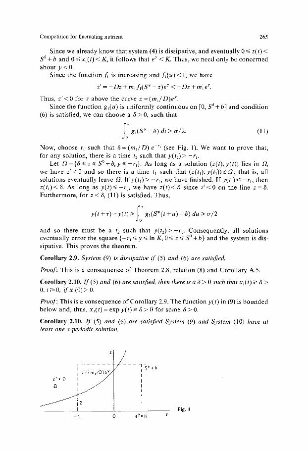
z' = - D z + mlf l (S* -- z)e y < - D z + ml e y.

Thus, z ' < 0 for z above the curve z -=(ml /D)e y. Since the funct ion g~(u) is uni formly cont inuous on [0, S ~ b] and condi t ion

(6) is satisfied, we can choose a 6 > 0, such that

fjg,(S*- a) > ~/2. (l l) dt

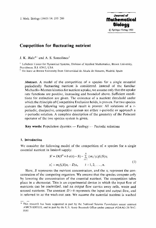
Now, choose rl such that 6 = ( m J D ) e -r, (see Fig. 1). We want to prove that, for any solution, there is a time t2 such that y ( t2 )> -r~.

Let ~2={6<~z<~S~ As long as a solution (z( t) ,y( t)) lies in ~ , we have z ' < 0 and so there is a time t~ such that ( z ( h ) , y ( t O ) ~ 2 ; that is, all solutions eventually leave ~2. I f y( t l )> - r b we have finished. I f y(tO<~ - r b then z( t i )<6. As long as y(t)<~-r~, we have z ( t ) < 6 since z ' < 0 on the line z = & Furthermore, for z < 6, (11) is satisfied. Thus,

y( t+ 'r ) -y( t )>~ g l ( S * ( t + u ) - ~ ) d u > ~ o ' / 2

and so there must be a t2 such that y ( t z ) > - r ~ . Consequent ly , all solutions eventually enter the square {-rx <~y~<ln K, 0 ~ < z ~ < S ~ and the system is dissipative. This proves the theorem.

Corollary 2.9. System (9) is dissipative if (5) and (6) are satisfied.

Proof: This is a consequence of Theorem 2.8, relation (8) and Corol lary A.5.

Corol lary 2.10. I f (5) and (6) are satisfied, then there is a 6 > 0 such that xl( t) >I ~ > O, t>~O, if xl(O)>O.

Proof: This is a consequence of Corol lary 2.9. The funct ion y(t) in (9) is bounded below and, thus, xl(t) = exp y(t)/> ~ > 0 for some 6 > 0.

Corollary 2.10. I f (5) and (6) are satisfied System (9) and System (10) have at least one "r-periodic solution.

Z

. . . . T . . . . . . .

I I z = ( r n l / D ] e ~ ""

z ' < O I

1

I - r ~ 0

- - - - 7 - - - - S ~ I

I I

t L q I I

I

e Y = K

Fig. 1 Y


Proof: Since the systems are dissipative and r-periodic, they have at least one r-periodic solution (see, for instance, Pliss [13, Ch. II, Th. 2.3] or Hale [4]).

Corollary 2.11. I f (5) and (6) are satisfied and the periodic solution o f (10) is unique, stable and a global attractor, then all solutions o f (11) tend to it.

Proof: This is a consequence of Corollary A.6.

3. E q u a l w a s h - o u t ra tes D = D t . . . . = D .

Let us make the following change of variable in Eq. (1')

(zo) f 1 !1() zl 0 1 0 xl

z2 = 0 0 1 x2 �9 "s . . . . . . . .

n 0 0 0 x~

Observe that

We obtain:

S = z 0 - ~ z~, z~=xi, i = l , 2 , . . . , n . i=1

Z'o = - D z o + D ( S ~ + be(t)) + ~ (D - Di)z~ i = l

t zi = z ig i ( zo-~ zi), i= 1 , . . . , n.

Since we already know that system (4), and consequntly system (1) are dissipative, the above system will also be dissipative.

As we have seen, the parameter D represents the input and output flow, and the D~ represent the wash-out rate plus the death rate of the corresponding species. If D is relatively large then the influence of death should be small compared to the importance of the wash-out. Thus, following Hsu, Hubell and Waltman [9] and H. Smith [14] we will assume that D = Dl . . . . . D,.

This assumption uncouples the first equation of the system and we obtain

Z'o = - D z o + D ( S ~ + be(t)) (12) !

Z i = z i g i ( z o - - ~ 7:i) , i = 1, 2 , . . . , n.

The first equation is the same as Eq. (3). Therefore, it has the unique periodic solution S*(t) which is globally asymptotically stable. Since Zo( t ) -S* ( t ) approaches zero exponentially, we obtain immediately for system (1):

Theorem 3.1. I f (S(t) , x l ( t ) , . . . , x~(t)) is a solution o f (1) in the case o f equal + n wash-out rates, then S ~ = l x ~ - S * ( t)-~O exponentially as t->oo.

Asymptotically in t, this has the following implication. When all species go extinct, we have S ( t ) = S*(t) as was expected, When they don't go extinct, we have the following "conservation law": At any moment of time, the sum of the


species plus the actual nutrient is equal to the nutrient that would be available in the absence of species.

Since we are interested in periodic solutions, and z*( t ) is globally asymptotically stable, we are going to make Zo(t) = S*( t ) and reduce the system to

z'i = zig~(Z*), i= 1 . . . . , n (13)

where we have denoted by Z * = S*-5~7=~ zi. Our objective is to study the asymptotic behavior of (13) and then use Lemma

A.4 to gain information about the asymptotic behavior of (12). Let us write system (13) as

and system (12) as

Y ' = F(t, Y) , (t3)

x ' = F(t, X) +R(t, X). (12)

We must obtain an estimation of R(t, X ) . We have proved already that the system (12) is dissipative. Every solution of the first equation of (12) can be written as

Zo(t) = S*(t) + C e n,

for some constant C. Substituting in the remaining equations of (12), we obtain

z~ = gi(S*(t) + C e o~ _ y. zi)zi

= zi{gi(S*-~ zi)d-(gi(S* q - a e Dt ~ zi)_gi(S. ~ zi))}

= z,g,(S* - Z z,) + R(t, z)

where z = ( z l , . . . , z,)- Assuming that g has a bounded first derivative, an application of the mean

value theorem shows there is a constant K such that

IR(t, z)[<~Ke-D~[zl foral l z.

Since (12) is dissipative, for any bounded set U in En, there is a constant C depending on B such that ]R(t, z(t))] ~< C e x p ( - D t ) for all solutions z(t) with z(0) ~ U.

With the definition of M ( F ) in the appendix, an application of Lemma A.4 yields

Theorem 3.2. Suppose (H1) and D = D~ . . . . . Dn. Then all the solutions o f the n + 1 dimensional system (12) approach asymptotically the set M ( F ) o f the n- dimensional system (13). In particular, i f (13) has a unique periodic solution which is stable and a global attractor, then all solutions o f (12) approach it.

From here on, we will concentrate on the study of system (13), which has interest of its own, bearing in mind that the information about its limit set is also information about the limit set of (12).


3.1. Competitivity

Extending M. Hirsh's ideas to n o n a u t o n o m o u s systems, we say that a system

x' = F(x, t) (14)

with F(x, t) a funct ion o f class C ~, defined in a domain I2 <~ R" is competitive if the entries DF~ of the Jacobian Matrix DF satisfy

D F 0~<0 for i C j and all t/> to.

We say that the system is cooperative if

DFo >~ O for all t >~ to and i # j.

We use the adjective strict if the inequalities are strict.

Theorem 3.3. The system (13) is competitive under hypothesis (H1) and strictly competitive under hypothesis (H2).

Proof: To calculate the Jacobian, observe that

dgi(Z*)/ dzi = dg,/ dZ* . dZ*/ dzi = g'~ ( Z * ) ( - 1) = -g l (Z*) .

The Jacobian is:

D F =

:g, (Z*)-g ' l (Z*)z l -g'l(Z*)Zl -g' l(Z*)z,

-g'z(Z*)z2 g2(Z*)-g'z(Z*)z2 -g~(Z*)zz

- g " (Z*)z, -g '~ (Z*)z , g,(Z*)-g ' , , z ,

Since the gi are increasing, g'i I> 0, and so, for all zi >/0, the system is competitive. I f the g'~ > 0, then the system is strictly competi t ive in z~ > 0.

The solutions o f (14) have certain monotonic i ty properties which are a consequence o f Kamke ' s Compar i son Principle. We use it in the form given by Hirsh [5].

Let x and y be n-vectors. We write x < y if x~ < y~, i = 1 , . . . , n. The vectors x and y are related if either x < y or x > y. They are unrelated if there exists i and j such that xi<~yi, xj>~y~, i # j .

Theorem 3.4 ( Kamke). Let F(x, t) be defined on a domain ~, which is the intersection of an open set and the closure of an open set (in particular R" and R+). Let x(t) and y(t) be solutions of (14) defined on a <~ t <~ b.

(i) I f (14) is cooperative and x(a)< y(a), then x(b)< y(b). (ii) I f (14) is competitive and x(a), y(a) are unrelated, then x(b), y(b) are also

unrelated.

For 2-dimensional systems, Kamke ' s theorem assumes a part icularly strong form that we state separately.

Theorem 3.5. Let n = 2. Let z( t) and y( t) be solutions of (14), yi( t) = zi( t) + hi(t). (i) I f (14) is cooperative and hi(a)> O, then hi(b)> O.

(ii) I f (14) is competitive and hi(a)~O, hj(a)~O, then hi(b)>~O and hj(b)<~O.

For strictly competi t ive systems, we can slightly improve on Kamke ' s theorem.


Theorem 3.6. Let n = 2 znd z(t), y(t) be two different solutions defined on [a, b]. I f (14) is strictly competitive and hi(a) >1 O, h2(a) ~< 0, then hi(t) > 0, h2(t) < 0, for all t in (a, b]. I f hl(a)<~O, h2(a)~O, then h i ( t )<0 , h2(t)>O for all to(a , b].

Proof: The variational equations are

h~ = Fi(xl + hi, x2 + h2)- Fi(Xl, x2)

aF, OF~ -Ox~i(xl +Ohbx2+Oh2)h, +ox-~2(Xl +Ohl, x2+Oh2)h2, 0<~0~<1. (15)

Let h~(a)= 0. Since the solutions are different, we have h2(a)< 0. From Eq. (15), we have

OF1 h~(a) = 7X2 (xl(a) -t- Ohl(a), x2(a) + Oh2(a))h2(a) > 0

because h2 (a )< 0 and OFi/Ox2<O. Thus, we have h i ( t ) > 0 for some time t > a. By continuity we have also h2( t )<0 for some interval of time. As long as h 2 ( t ) < 0 , hl(t ) cannot become zero because, if h i ( t 1 ) = 0 , then h ~ ( t l ) > 0 by the same reasoning as above. This leads to a contradiction. Similarly, as long as hi(t) > O, h2(t) cannot become zero. Finally, they cannot become zero at the same time because of the uniqueness. The second part of the theorem is proven the same way.

Remark: Theorem 3.6 admits the following geometrical interpretation. Let P--= (P1, P2) be a point in R 2. Define the 2nd quadrant relative to P by [P]2 = {(x, y): x > PI and y < P2}. Consider a moving frame of reference with z(t) at the origin. I f y(a) c Cl[z(a)]2 then y(t) c [z(t)]2 for all t c (a, b]. Here C1 denotes closure. Thus, if y(a) starts in the closed 2nd-quadrant relative to z(a), it would always remain in the open 2nd-quadrant relative to z(t) for t > 0.

For D = D1 = D2 and n =2, we have proved that all solutions of (12) are attracted to the integral manifold {(t, S, x): S ( t ) + ~ xi(t)= S*(t), t I>0} and the solutions on this manifold have certain monotonicity properties. For D1, D2 close to D, the solutions should also be on an integral manifold and conserve the monotonicity properties. It should be possible to give a proof of this using classical methods in the theory of integral manifolds (see, for example, Hale [2]) and the fact that the system is dissipative.

4. General 2-dimensional competitive systems

From here on, we will consider only the case of two competing species. In the previous section we saw, that for D = DI = D2, the 3-dimensional system (1) can be reduced to a 2-dimensional competitive system.

In this section, we will prove a very general result for 2-dimensional competitive systems. Applying this general result to our particular system (13) we will see that the dynamics of (13) are trivial, i.e. all solutions approach a periodic solution with the same period ~- as the input function e(t).

To investigate the solutions of a general cooperative or competitive system (14) for n = 2, we will make use of Poincar6 map T, or operator of translation


along the solutions, defined as follows: let z(t; Zo) be the solution of (14) with z(0) = Zo. If z(t; Zo) exists on 0<~ t ~ < T, we define Tzo = z(T; Zo), where T is the period of the input function e(t).

It is well known that the fixed points of T correspond to the r-periodic solutions of (14) and that the stability of the periodic solutions corresponds to the stability of the fixed points for the discrete dynamical system { Tk}, generated by T. The stability of a fixed point ~ of T is determined by the eigenvalues of the derivative D T of T at ~, which is the monodromy matrix of the system linearized around the periodic solution z(t; ~). We will assume (14) to be dissipative. In particular, every solution z(t, Zo) of (14) is defined for t >! O, z(z, Zo) exists and T is defined for all Zo.

Let us draw some conclusion from Kamke 's Theorem for the Poincar6 Map T. Let Q = (ql, q2) be a point in the plane. Define the open quadrants with respect to Q;

[ Q ] , = { ( x , y ) : x > q l , y > q 2 } , [ Q ] 2 = { ( x , y ) : x > q , , y < q 2 } .

[Q]3={(x,y): x < q l , y<q2}, [Q]4={(x,y): x < q l , y > q 2 } .

Also let C1 of a set denote closure.

Lemma 4.1 (Monotony of the Poincark Map). Let T be the Poincark Map of (14) defined on 12 as above.

(i) I f (14) is cooperative, i= 1 or 3 and TkOxo c Cl[ Tko-lxo]i, for some ko, then Tk+lXo e Cl[ Tkxo]i for all k > ko.

(ii) I f (14) is competitive, i= 2 or 4 and TkOxo ~ Cl[ Tk~ some ko, then Tk+lXo ~ Cl[ Tkxo]ifor all k >~ ko.

Proof: Let us prove part (ii). The proof of (i) is similar. I f Xo is a fixed point Txo = Xo, then Tk+lXo = Tkxo for all k and the theorem

is trivially true. Thus, assume Xo # TXo. We also assume TkOxo c Cl[Tko-~xo]2, since the other case is proved in the same way.

I f a = Tkoxo, b = Tk~ and a = b +h, then either hi > 0 or h2<0 and a and b are unrelated. Kamke 's theorem affirms that the solutions u(t, a) through a and u(t, b) through b are unrelated, i.e. if u(t, a ) = u(t, b)+h(t ) , then hl(t)>-O and h2(t)<~O.

Since the system is periodic, we have u(t, a ) = x ( t +koT, Xo) and u(t, b ) = x(t + ( k o - I)T, Xo). For t = T we obtain u(r, a) = u(T, b) + h(r) and so x((ko + 1)T, Xo) = x(koT, Xo) + h(r). Thus, Tko+lxo e Cl[ Tk~ An inductive argument com- pletes the proof.

Geometrically, the Lemma says that the Poincar6 Map preserves quadrants 1 and 3 for cooperative systems, 2 and 4 for competitive systems.

We can now prove the main result.

Theorem 4.2 (General cooperative or competitive systems). Let (14) defined on 12 be dissipative, i.e. all solutions eventually enter the ball B(R) and remain there. I f (14) is cooperative or competitive in B(R)c~ 12, then a solution is either a r-periodic solution or approaches a r-periodic solution as t-~ eo.

Proof: We can restrict ourselves to B(R) c~ 12 since we assume that solutions do not leave 12, and eventually enter B(R). Consider the case of a cooperative system.


Let Xo be a point o f B(R)c~ f2. I f Xo is a fixed point of T we have finished. Otherwise we have an alternative. Either we have Txo6 [Xo]i, i = 1, 3 or Txo~ Cl[xo]i, i = 2, 4.

In the first case, by repeated applicat ion o f Lemma 4.1 we would have Tkxo ~ [Tk-lxo]~, i = 1, 3, for all k. I f i = 1, this implies that both componen ts o f Tkxo are increasing sequences. Since the system is dissipative, they are bounded above, and so they tend to a limit ~j. Thus Tkxo ~ Yc, and ~ is a fixed point. I f i = 3, a similar a rgument proves the result.

In the second case, two things can happen. Either, for some ko, we have TkOxo c [Tk0-1Xo]~, i = 1, 3, and we are in the first case from there on. Or Tkxo Cl[Tk-~Xo]i, i = 2 , 4 for all k, and we can argue again as in the first case using part (ii) o f Lemma 4.1.

Thus, in any case, for each Xo there exists an ~ = T~, such that Tkxo ~ .~.

Corol lary 4.3. All solutions of system (13) approach a T-periodic one.

Proof: We saw that (13) was dissipative and competi t ive and thus, Theorem 4.2 implies the result.

5. Two species competition. The trivial solutions

Let us turn our at tention back to system (13) in the case of two compet ing species. We will assume H2, and so (13) is strictly competitive. A stronger version of Kamke ' s Theorem is valid (Theorem 3.6). We also can obtain a s t rengthened version o f Lemma 4.1.

Lemma 5.1 (Strict Monotony of the Poincar~ Map). Let T be the Poincar~ map corresponding to a strict competitive system (14) and i = 2 , 4 . I f Tkoxo E Cl[ Tk~176 for some ko, then Tk+lxo E [TkXo]i for all k > ko.

Proof: The same as in lemma 4.1.

Geometrical ly, if Tkxo is in the closed 2nd quadrant relative to T k ix0, then Tk+~Xo will be in the open 2nd quadran t relative to Tkxo.

It turns out that the Poincar6 map for (13) has the same monotonic i ty properties as the Poincar6 map for the Lotka-Vol ter ra equat ions studied by deMot ton i and Schiaffino [10]. Thus, we will be able to use the results o f these authors, as long as they depend only on the properties o f the Poincar6 map and not on the specific form o f the equations.

The fol lowing three Lemmas depend only the Poincar6 map and the proofs are given in deMot toni and Schiaffino [11, Lemma 4.2, 4.3, 4.4]. Let P be a fixed point o f T, TP=P. Define the region of attraction o f P by ~ / ( P ) = {Q~ R2 : T ~ Q ~ P}.

Lemma 5.2. I f P is a fixed point of T, then T([P]i\{P}) c [P]i, i = 2, 4.

Lemma 5.3. I f P is a fixed point ofT, then, for any Q ~ [ P ]i c~ sd( P), i = 2 (respectively i -- 4), we have [P]i c~ [Q]j ~ ~ ( P ) , j = 4 (respectively, j = 2). Moreover, if R, S c ~ ( P ) , then [R]2c~[S]4~ .;d(P).


Lemma 5.4. Let ~ c RZ+ be a T-invariant curve which is a nondecreasing graph. Then Y, is the graph of a strictly increasing function.

5.1. Trivial periodic solutions

We say that a solution is trivial if at least one species is identically zero. We shall a ssume that there is no extinction due to lack of food; that is,

Iog i (S*( t ) ) > 0, i = 1, 2. (16) dt

I f we linearize a round the z-per iodic solut ion (0, 0), we obtain the matr ix for the l inearized equat ion as

The characteris t ic mult ipl iers are exp So gi(S*) dt > 1, i = 1, 2. Thus, the origin is total ly unstable for the Poincar~ operator .

Let us now make Zl = 0 or z2 = 0 and investigate the resulting one-d imens iona l system.

Theorem 5.5. For n = 1, and H2 system (13) has a unique nontrivial periodic solution which is globally asymptotically stable i f (16) is satisfied.

Proof: The Poincar6 m a p is mono tone in the one-d imens iona l case. Since the system is dissipative and the origin is repulsive for the Poincar6 map , there is a nontr ivial fixed point o f T.

We prove nontrivial per iodic solutions are asymptot ica l ly stable. Indeed, the linear variat ional equat ion for a periodic solution z is

y ' = [ g , ( S * - z , ) - gl ( S* - z~)z~]y.

Now, a necessary condi t ion for Zl(t) to be per iodic is that

f[ g,(S*- z,(t)) = dt O.

Thus, the characterist ic mult ipl ier is exp So -g'~ (S* - Zl)Z~ < 1, since g'~ > 0. The monoton ic i ty of the Poincar6 m a p implies that there is a unique fixed point 2~ of T. Since we know that all solutions tend to a r -per iodic solution and the origin is total ly unstable, all solutions tend to ~l. This proves the theorem.

Corol lary 5.6. Suppose system (1) satisfies (H2) , D = D i for all i and So g~( S*( t)) dt > O. I f the species x2, . . . , x, go exponentially extinct, then all solutions except ( S*( t), 0 , . . . , O) approach a unique z-periodic, globally asymptotically stable solution (S*(t), x~(t), 0 , . . . , 0).

Proof: This follows f rom Theorem 3.2 and Theo rem 5.5.

Remark: The existence of at least one nontrivial z-per iodic solut ion was proven by Hsu [7] for M - M systems. The uniqueness and asympto t ic stability were p roven for M - M systems by a different me thod by H. Smith [13].


Under Hypothesis (H2) the system (13) for n = 2 has only three trivial solutions (0, 0), (~(t) , 0) and (0, ~2(t)).

Let us now study the stability properties of (~, 0). The variational equation around (~l(t), 0) is

y , = ( [ g l ( S * - ~ , ~ g ' l ( Z * ) ~ l -g'~(Z*)~l(t)] y.

g2(S*- ~) /

The multipliers of this system are eXpSo--g'l(S*--zO~l(t) d t < l and exp So g 2 ( S * - z l ( t ) ) dt. Thus the stability depends on the sign of

d e f ~" ~r

I(~,) = Jo g2(S(t)) dt, (17)

where we have substituted S * - ~ ( t ) = ~(t), since S ( t ) + ~ ( t ) = S*(t).

Theorem 5.7. The fixed point (~l, O) of T is asymptotically stable if I(f~) < 0 and it is unstable if I( ~i) > O. A similar result is valid for (0, Zz)-

Remark: For M-M systems, this is Lemma 3.1 in H. Smith [13]. He assumes S( t) = S o + bS~( t) + b 2 S2( t) �9 �9 �9 and substitutes in I(Zl) = 0 to obtain, in parameter space, the neutral stability curve. He then finds a value of b for which there is a loss in stability and periodic solution bifurcates from (S(t), ~(t), 0). We are not going to follow this line of inquiry, because among other things, we don't assume a particular form for the functions gi or the input function S~ be(t).

5.2. Regions of attraction

Theorem 5.8. Let ( ~, O) be asymptotically stable ( I ( ~) < 0). The region of attraction sg ( zl, O) includes the positive xl -axis. I f ( Zl, O) is not globally asymptotically stable in the strictly positive quadrant QO, then the boundary of ~r in QO is the graph of a strictly increasing T-invariant curve u(x 0 such that u(O)= O. I f u(a 0 = + ~ for some a~ > O, then all points satisfying Xl > al are in Jg(zl, 0).

Proof: This depends only on the monotonicity of T. See de Mottoni and Schiaffino [11, Th. 4.7].

A similar theorem is valid for the fixed point (0, ~2), assuming it is asymptotically stable. See de Mottoni and Schiaitino [11, Th. 4.7].

We have seen that the origin is totally unstable, which means that, for the time reversed system, it is asymptotically stable. We define the region of repulsion .ff-~(0) of the origin to be the region of attraction of the Poincar6 map for the time reversed system. The time reversed system is cooperative and the Poincar6 map has also the monotonicity properties. Following de Mottoni and Schiaffino [11, Th. 4.4], one can prove

Theorem 5.9 (Region of repulsion of the origin). The boundary of ~l-I(O) consists of the segments [0, Zk], k = 1, 2 in the respective axes and the graph F of a strictly decreasing continuous function connecting (0, z2) with (~, 0).

This curve F is very important since we show in the next section that all positive fixed points of T are in F.


6. Two species competition. Nontrivial solutions

6.1. Location of the non-trivial fixed points of T

We need the following lemma which is a private communication of P. de Mottoni.

Lemma 6.1. I f P and Q are fixed points of T, then P~ [Q]3, P~ [Q]I.

Proof: Let P ~ [Q]3. By Kamke's theorem z(t, P) ~ [z(t, Q)]3 for all t > 0. Indeed, if for some tl, we had z ( h , P) ~ Cl[z(tl , Q)]i, i = 2, 4, then, for all t > fi, the same would be true. But that contradicts the fact that z(~-, P )~ [z(~', Q)]3 .

Now since z(t, P) and z(t, Q) are periodic we get the equations

o r g i ( S * - ~ z j ( t , P ) ) d t = O i = 1 , 2

(18) oTg,(S*-Zzj ( t , Q)) dt=O i = 1,2.

But, if z(t, P)~[z( t , Q)]3, then zi(t, P)<zi( t , Q), i= 1,2 and S * - Y . zi(t, P ) > S * - ~ zi(t, Q). Since the gi are increasing functions,

f o{g~( S* - Z zj( t, P)) - g,( S* - Z zj( t, Q))} dt > 0

which contradicts Eqs. (18). The same proof applies to P~ [Q]I.

Theorem 6.2. All nontrivial fixed points of T lie on the curve F defined in Theorem 5.9.

Proof: Suppose Q = (ql, q2) is a fixed point above the curve F. By the Lemma 6.1, there cannot be fixed points in [(zl, 0)]1 or [(0, z2)]1 and so we have ql ~< Zl and q2 ~< z2. By Lemma 5.1, there is no fixed point P = (pa, P2) # Q such that Pl = ql or P2 = q2. Thus, q~ < zl and q2 < z2. Let (vl, q2) and (q~, v2) be the points on F with respectively the same abscissa and ordinate as Q. By Lemma 6.1, there are no fixed points in the rectangle with vertices Q, (vl, q2), (q~, v2), (v~, v2). Let P be the first fixed point on F with p, < vl, p2 > q2 and let S be the first fixed point on F with sl > q~ and s2 < v2. Thus, Q ~ [P]2 c~ [S]4. But either P or S attracts the whole rectangle [P]2 c~ [S]4. Indeed, all points on the segment of the curve between P and S are attracted to P or S because of the monotony of T. I f it is S, then, for any point R in the segment, R ~ ~ (S) , and JR]2 c~ [S]4 c sO(S) by Lemma 5.3. Thus Q is not a fixed point. I f the points between P and S on F are attracted to P, the same argument applies to complete the proof of the theorem.

Corollary 6.3. All solutions of (13) for n = 2 eventually enter the rectangle with vertices (zl, O) and (0, 22).

As a consequence of Theorem 6.2, we can give some sufficient conditions for the existence of nontrivial periodic solutions.

Theorem 6.4. I f both fixed points (zl, O) and (0, ~2) are stable or both unstable, then there is at least one nontrivial fixed point in F. Moreover, if both are unstable and there is a finite number of fixed points, one of them must be locally asymptotically stable.


The proof depends only on monotonicity. See de Mottoni and Schiaffino [11, Th. 5.23.

Theorem 6.5. I f I(2i) is defined in (17), 1(21)<0 and 21 is not globally attracting, then there is a least one nontrivial fixed point in F.

Proof: I f ~ is the boundary of the region of attraction of (zl, 0), then ~ is a T-invariant and strictly increasing curve, which would intercept the T-invariant and strictly decreasing curve F. The common point is a nontrivial fixed point for T.

6.2. A condition to ensure a fn i te number of fixed points

If w = (u, v) is a fixed point of T, we have

(T(u, v))l = u (19) ( T(u, v))2 = v.

I f one could use the implicit function theorem in (19), one could find functions v = U(u), and u = V(v) such that (T(u, U(u)))l = u and a similar equation for the v. The fixed points would be the intersections of the curves U(u) and V(v). I f these functions are analytic, we shall see that only a finite number of intersections can occur.

In order to use the implicit function theorem on (19), we need the derivative T'(u, v). But this is the monodromy matrix of the linearized equations

([gl(u*, v*) - g'l (u*, v*)u] -g'l (u*, v*)u ) y ' = \ -g'z(U*, v*)v [gz(u*, v*)-g~(u*, v*)v]_ Y" (20)

Where we have let (u*, v*)= S * - u - v . I f Y(t) is the solution with Y(0)= co l ( I ,0 ) , we have y~(0 )<0 since -g' lu<O. I f y l ( t 0 = 0 for some tl, we have Y'I (tl) > 0. Thus, this solution remains strictly in the 2nd quadrant. Similarly, one can prove that the solution with Y(0)= col (0, 1) remains strictly in the 4th quadrant. Thus, we have

Lemma 6.6. The monodromy matrix of system (20) has strictly positive diagonal elements and strictly negative off-diagonal elements.

One can use now the implicit function theorem to prove

Lemma 6.7. There are two continuous functions U(u) and V(v) defined for u in (0, 21) and v in (0, 22] such that U(zO = 0 and V(z2) = O, and

(T(u , U(u)))l = u, ( T ( V ( v ) , @)2= v. (21)

I f the functions f are analytic, then U and V are analytic.

Theorem 6.8. I f the functions f are analytic, and I(21)" I(2z) # O, there is a finite number of fixed points of the Poincard map.

Proof: We know that all possible fixed points are on the curve F. Since 1(21)- 1(22)# 0, we have that (21, 0), is either asymptotically stable or unstable, and that there is a region of attraction or repulsion in which there are no fixed


points . The same is t rue for (0, z2). Thus, the add i t i ona l fixed po in ts o f T are in the in te r io r o f F. Let 0 < r and 0 < s be such tha t there are no fixed poin ts for 0 < u < r and 0 < v < s. The funct ions U and V are def ined and ana ly t ic at least in (r/2, ~) for U and ( s /2 , :~2) for V.

Assume there are an infinite n u m b e r o f fixed po in ts o f T. By the reason ing above, they accumula te in the in ter ior o f F. Thus, the curves v = U(u), u = V(v) in tersect an infinite n u m b e r o f t imes. Since they are analyt ic , they are ident ical , which impl ies that every po in t on the curve v = U(u) is a f ixed point . Thus, this curve co inc ides with F for u ~ [r/2, ~ ] and v c [s/2, 32]. But that con t rad ic t s the fact that there are no fixed poin ts in F, for u < r and v < s.

Corollary 6.8. If the f are analytic and I(~1)" 1(32)> O, then there is at least one asymptotically stable .r-periodic solution of (13) for n = 2.

Proof: From Theorem 6.4 and Theo rem 6.8.

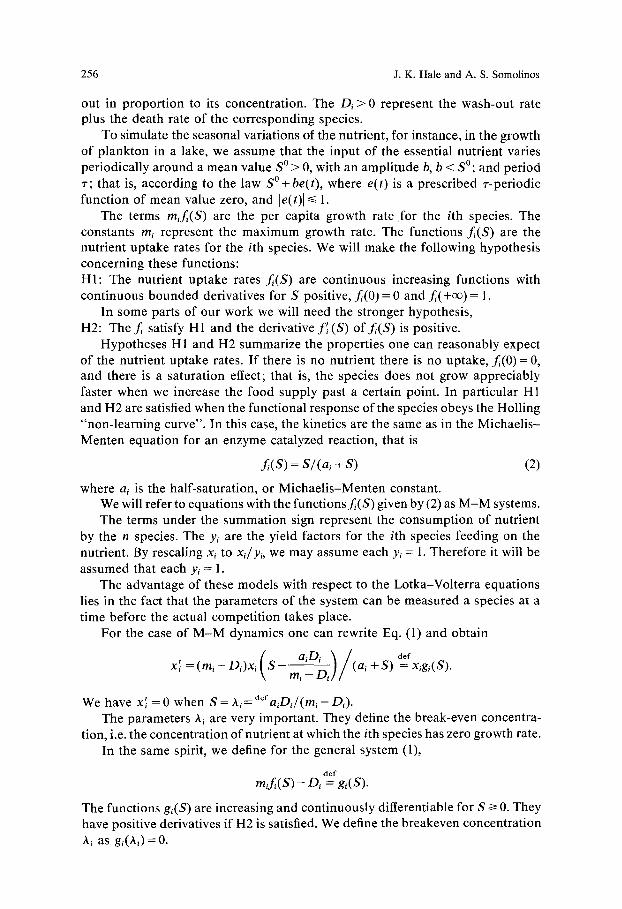
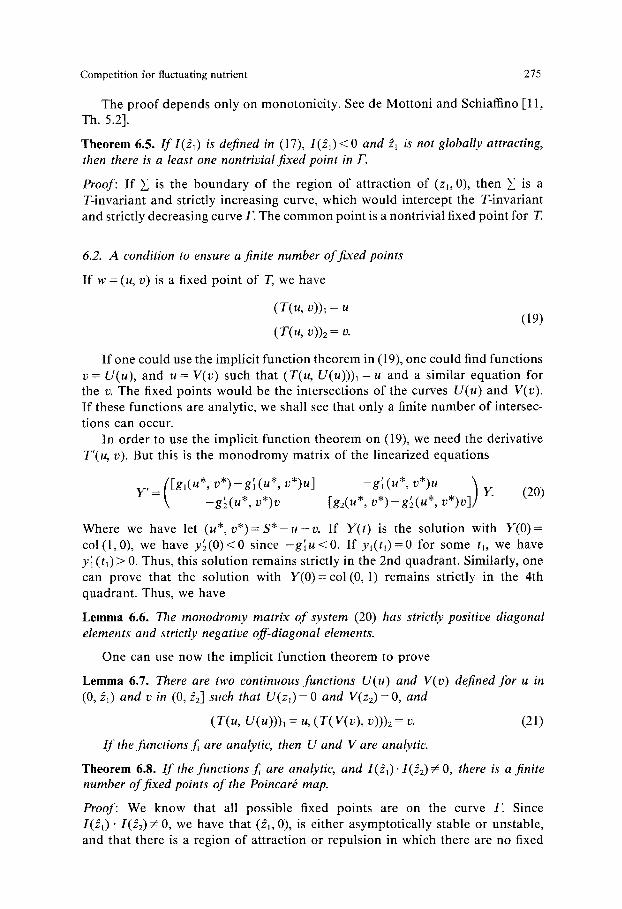
Theorem 6.9. Assume there are a finite number of fixed points of T. Then the regions of attraction of the stable fixed points of T partition R2+. The separatrices between the regions of attraction are the stable manifolds of the unstable fixed points (they are all saddles). These stable manifolds are the graphs of continuous increasing functions qb(ul) such that c~(O)= O.

The p r o o f is as in de Mot ton i and Schiaffino [11, Th. 5.8], see Fig. 2.

Fig. 2

P~P2P3 STABLE F.R (O,~'2)~L,~. / Q~Q2 UNSTABLE F.P.

(~, ,01

Fig. 3

7 / . . . .


6.3. Conclus ions about the original sys tem (12)

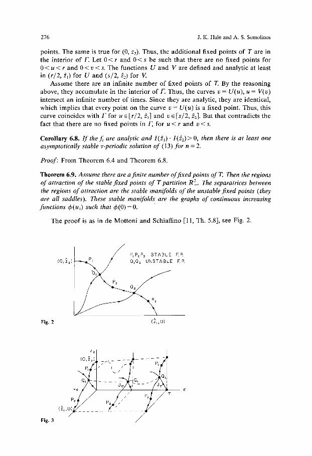
T h e o r e m 6 .2 g ives i n f o r m a t i o n a b o u t t h e m a x i m a l i n v a r i a n t se t M o ( F ) of t h e

P o i n c a r 6 m a p TF of ( 1 3 ) ( see t h e A p p e n d i x ) . F o r a n y o t h e r s t a r t i n g t i m e o-, t h e

se t M o ( F ) w o u l d h a v e t h e s a m e q u a l i t a t i v e f e a t u r e s , so t h e se t M ( F ) w o u l d l o o k

as i n d i c a t e d in Fig. 3. S i n c e M ( F ) is i n v a r i a n t f o r TF, i t is p e r i o d i c , i.e. M o ( F ) is i d e n t i c a l w i t h M , ( F ) a n d w e n e e d o n l y d r a w t h e i n t e r v a l [0, ~].

L e m m a A.4 a s s e r t s t h a t al l s o l u t i o n s o f t h e p e r t u r b e d s y s t e m (12) a p p r o a c h

a l so t h e se t M ( F ) . W e w a n t to p r o v e t h a t t h e y a p p r o a c h a spec i f i c p e r i o d i c

s o l u t i o n a n d d o n o t w a n d e r b e t w e e n t w o o f t h e m .

T h e o r e m 6.10. I f the periodic solutions o f (13) are f in i te in number, then every

solution o f (12) approaches one o f them.

Proof: L e m m a A.4, we k n o w t h a t t h e to - l imi t se t o f a n o r b i t o f t h e d i s c r e t e

d y n a m i c a l s y s t e m d e f i n e d b y t h e P o i n c a r 6 m a p TV+R f o r (12) m u s t c o n t a i n f ixed

p o i n t s o f TF. I f i t c o n t a i n s o n l y o n e p o i n t , we a re f i n i s h e d . S u p p o s e it c o n t a i n s

m o r e t h a n o n e f ixed p o i n t o f TF. T h e n it m u s t c o n t a i n a n a s y m p t o t i c a l l y s t a b l e

f ixed p o i n t o f TF. N o w a n a r g u m e n t s i m i l a r to t h e p r o o f o f L e m m a A.4 s h o w s

t h a t it c a n c o n t a i n o n l y t h e s t a b l e one . T h i s c o m p l e t e s t h e p r o o f .

Acknowledgment. We wish to thank P. de Mottoni, for several suggestions; in particular, for a generalization of Theorem 3.6 to its present form. The authors also are very grateful to the referees for their constructive criticism of the original manuscript.

Appendix. Dissipative systems

Consider the n-dimensional vector equation

17= F(Y, t) (22)

defined in R x,O, where ,O is a domain in R' . We assume that F(Y, t) is continuous in t, Y, together with its first derivative in Y, is T-periodic in t and the solution Y(t, to, Yo) through the point (to, Y0) exists for t ~ > t o and is unique. This implies that the solutions depend continuously on (t, to, Yo).

Let T:/2 c R" -> R" be the Poincar6 map, TY o = y(% 0, Y0). We say T is d&sipative if there is a bounded set B _~ R" such that, for any Y c D, such that T ' Y ~ ~2, there is an integer n o = no(Y, B) such that T"YE B for n/> no(Y , B). Since the solution Y(t, to, Yo) of (22) depends continuously on (t, to, 1Io), one can show that T is dissipative if and only if system (22) is dissipative.

Let d(K, M) be the distance from a set K to a set M, d(K, M)=sup{d(y, M),y6 K} where d(y, M)=sup{ ly-x l : x c M}. A set M c R" is said to be invariant under T if TM=M. A compact invariant set M is said to be maximal compact invariant if, for any compact invariant set K c R' , we have K c M. An invariant set M is stable if for any e > 0, there is a 3 > 0 such that, if d(y, M) < 8, then d(Tny, M ) < e if n/> 0. A set M attracts a set K if d(T"K, M)-> 0 as n -> co. An invariant set M is uniformly asymptotically stable if it is stable and there is an open neighborhood V of M such that M attracts V.

A fundamental result on dissipative systems is the following

Lemma A.I. I f T is dissipative, then there is a maximal compact invariant set J of T which is uniformly asymptotically stable and attracts bounded sets.

Proof: We first show there is a compact set K with the property that, for any compact set H, there is a neighborhood H 0 of H and an integer N(H) such that T"HoC_ K for n>~ N(H). In fact since T is dissipative, there is a bounded set B (which may be taken as an open set) such that T'y ~ B for n >1 no(y , B). We suppress the dependence on B since it will remain fixed. By continuity of T, there


is an open neighborhood Oy of y such that T"o~-~)Oy ~_ B. Suppose H is an arbitrary compact set of R n. The sets {Oy, y ~ H} form a covering of H and have a finite subcovering {Oy~, i = 1,2 . . . . , p}. Let N ( H ) = max {no(y~), i = 1, 2 . . . . , p}. Then T"o~'~)Oy~ ~ B an_d 0 ~ no(yl)~ N(H) . Let/~ be the closure of B, H o = U~O,~ and let K be the union of/~, T/~, . . . . TN~B)B. We claim that Tn/~c K for n ~> N(/~). In fact, let y ~/~, n t> N(/3). If T"y E/~, we have finished. Assume T"y~ B, then there is an integer j such that 0 < j ~< n and T" @ c/~ and T"-ky~ B for 0 ~< k <j. But T"-Jy e Oy~ for some i, Tn~ B, 0<~ n(yi)<~ N(B). This implies O<j<~ n(yi)<~ N(B) and so T~y ~ K for n/> N(/~). Let / ~ ( H) = N ( H ) + N ( B ) and suppose y e Ho, n t>/q(H). Then y c Oy~ for some i, 0 ~ n (yl) <~ N ( H ) and T "(y~) Oy, c /~. Therefore, T"Oy~ = T "-"(y~) T ~(y~) Oy~ ~_ K for n/> N ( H ) . This proves the assertion at the beginning

of this paragraph. if y + ( K ) = U,~oT"K, then TN(O)+I/~ ~/~ implies that y + ( K ) c K and so is precompact. This

implies the w-limit set o)(K) of K, w(K) = (")m~ o Cl((._Jn~ m T"K) is compact and invariant. It is then immediate that w(K)c_ K. One can show that this implies w ( K ) = ( ~ , ~ o T~K. Let J = w ( K ) . We claim that J is independent of the set K which attracts compact sets of R". In fact, designate J by J (K) and suppose Kj is any other compact set which attracts compact sets of R n. Then there is an integer no(k, Ki , e) such that d(T"J (K) , K I ) < e, d(K, T"J(KI) )< e if n/> no(K , K1, e). Since J (K) and J(K~) are invariant, this implies J (K) ~ _ K~, J(KI)_~ K and J(K)~_ T'~Kt, J(KI)~_ T"K for all n/> 0. Thus, J ( K ) = J ( g l ) and J is independent of K.

To prove J is maximal, suppose H is any compact invariant set. Since K attracts H, for any e > 0, there is an integer n~(H, e) such that d(T"H, K ) < e for n~na(H , e). Since H = T " H for all n, we have d ( H , K ) < e for all e > 0 . This implies Hc_K. Thus, H~_ T"K for all n~>0 and, since J = ['-'l~o T"K, this implies H _~ J.

To prove J is stable, suppose the contrary. Then the compactness of J implies there is an e > 0 (as small as desired), a sequence of integers njooo, y j ~ y ~ J as j ~ o o such that d(T~yj, J ) < e , 0<~ n <~ n~, d(T~ J)>~ e. The set H ={y, yj, j>~ 1} is compact, y+(H) is precompact, J attracts H and w(H)~_ J. Thus, we may assume T"~y~ ~ z as j ~ oo. But z e w(H)~_ J which is a contradiction

since Tz ~ w(H) ~_ J and d(Tz, J)>~ e. The fact that J is uniformly asymptotically stable and attracts bounded sets follows from the fact

that J = w(K) and K attracts bounded sets. This proves the lemma.

Let us now interpret these results for Eq. (22). Let J be the set in Lemma A.I and define M(F)~_ R x R" by the relation M(F)={( t , Y): Y = Y(t, O, Yo), Yo e J, t ~ R} where Y(t, O, Yo) is the

solution of (22) through (0, Yo)- The set M ( F ) is invariant with respect to (22); that is, if (to, Yo) ~ M ( F ) , then (t, Y(t, to, Yo)) ~ M ( F ) for t ~ R. If we define the cross section M~(F) of M ( F ) at o- as

M~(F) = { Y: (o-, Y) ~ M(F)},

then the periodicity of F( Y, t) in (5) implies that M~+,(F) = M~(F) for all o- ~ R. Note that Mo(F ) = J. We can now prove

Lemma A.2. The invariant set M ( F ) o f (22) is uniformly asymptotically stable in R x R ~ and attracts any set o f the form R x B where B is bounded in R ~. Also, for any compact set Q c R ~, there is a constant K > 0, depending on Q, such that

]d(Y, Mr(F)) - d( ~ M,( F)) I <~ Ki t - s]

for t , s e R , Y e Q .

Proof The stability properties of M ( F ) follow from Lemma A.1 and the periodicity of F(Y, t) in r The estimate on d( Y, M,(F)) follows from the relation M~+,( F) = Y(tr + t, ~r, M~(F)) and the dependence of Y(t, to, Yo) on (t, to, Yo).

Since the set M(F) is asymptotically stable, one expects to find a Liapunov function ensuring this stability. If this Liapunov function is Lipschitzian we can use it to study perturbations of the system. The following Lemma affirms the existence of such a function.

Lemma 2.3 and the results of Yoshizawa [15, Theorem 22.3, p. 113] imply

Lemma A.3. I f system (22) is dissipative and M ( F ) is the invariant set for (22) defined above, then there is a function V(t, x) defined and continuous on ~ • ~" which satisfies

(a) V(t, Y) = 0 for (t, Y) ~ M(F) .

Competi t ion for fluctuating nutr ient 279

(b) There is a continuous increasing positive function a(r) ~ oo as r ~ oo and a continuous function b(r)~O as r ~O such that

a(d(Y, Mt(F))<~ V(t, Y ) ~ b(d(Y, M,(F))

for all (t, Y ) ~ •

(c) For any bounded set B c ~n, there is a constant L, depending on B such that

IV( t , Y ) - V ( t , V')] ~< L I V - V'l

for all t ~ ~, Y, Y ' c B. (d) V'(22)(t, Y ) < ~ - c V ( t , Y )

where c is a positive constant and

- - 1 V(22)(to, 1Io) = hliom+ ~[ V(to, �9 Y(to+h, to, I io))- V(to, Yo)]

where Y(t , to, Yo) is the solution of (22) through (to, Yo).

In our paper we encounter repeatedly the following situation: As t-+ +c~, some terms in the equations describing the evolution of the system decay exponentially, and the resulting "limiting equation" describes a dissipative system. The fact that this limiting equation is dissipative will allow us to get information about the asymptotic behavior of the original system. Indeed, Lemma A.3 can be used to compare the solutions of a perturbed system

2 = F(X, t) + R(X, t) (23)

to the solutions of (22). In fact, the derivative ~r(23) along the solutions of (23) is easily seen to be

12(23)(t, X) ~< 1;'(22)(t , X ) + LR(X, t) <~ -cV( t , X ) + LR(X, t),

o r

fo t

V(t, x(t))<~ e-C'V(0, X(0)) + L e-C('-S)R(X(s), s) ds.

Assuming further properties on R(X, t), one can obtain bounds on V(t, X( t ) ) and then use part (b) of Lemma 2.4 to obtain estimates on X(t) . For the applications that we have in mind, the function R(X, t) satisfies the property that, for any bounded set B c ~", there is a constant C depending on B and e > 0 independent of B such that

IR(X(t) , t)l ~< C e ~', t>~O (24)

for all solutions X( t ) with X(0) E B. Now suppose that (22) is dissipative. For any compact set B c E", let Xo~ B, and X ( t ) = X(t , 0, Xo) be a solution of (23). We have

V(t ,X( t ) )<~e-c ' [V(O, Xo)+LCfo 'e (C-~)Sds ]

<~ e-Ct[ V(O, X o ) - L C / ( c - e)] + e-~tLC/(c - e)

and V(t, X (t)) -> 0 as t ~ oo uniformly for X 0 c B. This implies, from (b) of Lemma 2.4 that X(t) ~ M ( F ) uniformly for X 0 ~ B. We have proved the following

Lemma A.4. Suppose (22) is dissipative, M ( F ) is defined as before in Lemma A.2 and R(X, t) satisfies (24). Then, for any compact set B ~_ R ' , the solution X ( t, to, Xo) o f (23) satisfies X ( t, to, Xo)-> M ( F) as t->oo uniformly for Xo~ B.

Corollary A.5. I f system (22) is dissipative, then system (23) is dissipative.

Corollary A.6. I f the hypotheses o f Lemma A.4 are satisfied and (22) has a unique z-periodic solution dg(t) which is stable and a global attractor, then all solutions o f (23) approach this z-periodic solution.

Proof: The hypothesis implies M ( F ) consists of {(t, qS(t), t c R}.

For more information about the comparison of solutions of (22) with solutions of (23) under conditions weaker than (24), see LaSalle [10], Artstein [1].


References

1. Artstein, Z.: Limiting equations and stability of non-autonomous differential equations. Appendix A in J. P. LaSalle, The stability of dynamical systems, SIAM Regional Conf. Series in Applied Mathematics, no 25, SIAM, Philadelphia, 1976

2. Hale, J. K.: Ordinary differential equations. Kreiger, 1980 3. Hale, J. K.: Theory of functional differential equations. Berlin-Heidelberg-New York: Springer,

1977 4. Hale, J. K.: Some recent results on dissipative processes. Lecture Notes in Math., vol. 799.

Berlin-Heidelberg-New York: Springer, 1980 5. Hirsch, M.: Systems of differential equations which are competitive or cooperative 1: Limit sets.

SIAM J. Math. Anal. (1982) 6. Hirsch, M.: Systems of differential equations which are competitive orcooperative 1I: Convergence

almost everywhere. (To appear) 7. Hsu, C. B.: A competition model for a seasonally fluctuating nutrient. J. Math. Biology 9, 115-132

(1980) 8. Hsu, S. B.: Limiting behavior for competing species. SIAM J. Appl. Math. 34, 760-763 (1978) 9. Hsu, S. B., Hubbell, S. P., Waltman, P. E.: A mathematical theory for single nutrient competition

in continuous cultures of micro-organisms. SIAM J. of Appl. Math. 32, 366-383 (1977) 10. LaSalle, J. P.: The stability of dynamical systems. Regional Conference Series in Applied Math.

no 25, SIAM, Philadelphia, 1976 11. Mottoni, P., de Schiaffino, A: Competition systems with periodic coefficients. A geometric

approach. J. Math. Biol. 11,319-335 (1981) 12. Pliss, V. A.: Non local problems in the theory of oscillations. New York: Academic Press, Inc., 1966 13. Pliss, V. A.: Integral manifolds for periodic systems of differential equations (Russian) Nauka.

Moskva, 1977 14. Smith, H. L.: Competitive coexistence in an oscillating chemostat. SIAM J. Appl. Math. 40 (No.

3) (1981). 15. Yoshizawa, T.: Stability theory by Liapunov's second method. The Math. Society of Japan, 1966

Received December 17, 1982/Revised September 28, 1983

Documents

Competition for fluctuating nutrient