Embed Size (px)
Citation preview

COMPETITION BETWEEN MICROFINANCE
INSTITUTIONS AND THE FORMAL BANKING SECTOR
by
TIA JANE MONAHAN
A THESIS
Presented to the Department of Economics
and the Robert D. Clark Honors College
in partial fulfillment of the requirements for the degree of
Bachelor of Science
June 2017

ii
An Abstract of the Thesis of
Tia Jane Monahan for the degree of Bachelor of Science
in the Department of Economics to be taken June 2017
Title: Competition Between Microfinance Institutions and the Formal Banking Sector
Approved: _______________________________________
Alfredo Burlando
Microfinance Institutions (MFIs) lend to impoverished communities with the
goal of spurring increases in income, consumption, business activity, and decision
making power. My research looks at how the formal banking sector responds to MFI
branch entry. I use data from a randomized control study done by Banerjee et al. (2013)
which allows me to control for endogeneity biases associated with MFI entry. I look at
how bank loan take-up and bank loan amounts change over the course of the study as
well as how clientele characteristics compare between those that borrow from banks and
MFIs. I find no significant differences in bank loan take-up or bank loan amount
between treatment and control areas, suggesting the banking sector does little to
respond to competition from MFIs. I test this zero effect on a variety of different
variables and parameters via a multitude of difference in difference estimators and I
reach the same zero-effect conclusion. I find multiple significant differences in
characteristics between MFI and bank borrowers. I conclude that MFIs and the formal
banking sector operate in relatively separate marketspaces with little to no competition.

iii
Acknowledgements
I thank Professor Burlando for helping me at every step of my thesis and taking
his time to be an active advisor throughout this process. I also thank Professor
Chakraborty for serving as my second reader and Professor Frank for serving as my
CHC thesis advisor. I also give big thanks to my roommates for putting up with me
daily throughout this process, and to my parents for their constant support during every
stress-induced, frantic phone call. Lastly, I send a huge thank you to the understanding,
accommodating, and supportive community of peers and mentors I have developed here
at the University of Oregon, all of whom have helped me through not only the thesis
process but my entire undergraduate career.

iv
Table of Contents
Introduction 1
Finance and the Poor 3
Microfinance 5
Area of Exploration 8
Literature Review 8
Data 12
Methodology 15
Results 22
Banking Sector 22
Previous Banking 24
Business Activity 25
Debt 26
Expenditures 27
Literacy Rates 27
Informal and MFI sectors 28
Informal 28
MFI 29
Characteristics of MFI and Bank loan take-up 30
Significant Borrower Characteristics 31
Significant Differences in Borrower Characteristics 32
Discussion 34
Conclusion 42
Tables 44
Bibliography 64
v
List of Tables
Table 1: Dependent Variable Means Across Measurement Periods .............................. 14
Table 2: Value Indicator Variable Cutoffs ..................................................................... 17
Table 3: Summary of Banking Sector Treatment Differences ....................................... 22
Table 4: Summary of Key Mean-Cutoff Value Indicator Variable Coefficients ........... 23
Table 5: Banking Sector – Treatment Differences from Baseline to Endline1 .............. 44
Table 6: Banking Sector – Treatment Differences from Baseline to Endline2 .............. 45
Table 7: Banking Sector – Effects of Previous Banking Differences between Treatment
and Control from Baseline to Endline1 on Bank Loan take-up ..................................... 46
Table 8: Banking Sector – Effects of Previous Banking Differences between Treatment
and Control from Baseline to Endline1 on Bank Loan Amount .................................... 47
Table 9: Banking Sector – Effects of Business Differences between Treatment and
Control from Baseline to Endline1 on Bank Loan take-up ............................................ 48
Table 10: Banking Sector – Effects of Business Differences between Treatment and
Control from Baseline to Endline1 on Bank Loan Amount ........................................... 49
Table 11: Banking Sector – Effects of Debt Differences between Treatment and Control
from Baseline to Endline1 on Bank Loan take-up ......................................................... 50
Table 12: Banking Sector – Effects of Debt Differences between Treatment and Control
from Baseline to Endline1 on Bank Loan Amount ........................................................ 51
Table 13: Banking Sector – Effects of Expenditure Differences between Treatment and
Control from Baseline to Endline1 on Bank Loan take-up ............................................ 52
Table 14: Banking Sector – Effects of Expenditure Differences between Treatment and
Control from Baseline to Endline1 on Bank Loan Amount ........................................... 53
Table 15: Banking Sector – Effects of Literacy Rate Differences between Treatment and
Control from Baseline to Endline1 on Bank Loan take-up ............................................ 54
Table 16: Banking Sector – Effects of Literacy Rate Differences between Treatment and
Control from Baseline to Endline1 on Bank Loan Amount ........................................... 55
Table 17: Banking Sector – Robustness Table, Value Indicator Variable Triple
Interaction Coefficients .................................................................................................. 56
Table 18: Informal Sector – Treatment Differences from Baseline to Endline1 and
Endline2 .......................................................................................................................... 57
Table 19: Informal Sector – Value Indicator Variable Triple Interaction Coefficients for
Endline1 .......................................................................................................................... 58
Table 20: MFI Sector – Treatment Differences from Baseline to Endline1 and Endline2
........................................................................................................................................ 59

vi
Table 21: MFI Sector – Value Indicator Variable Triple Interaction Coefficients for
Endline1 .......................................................................................................................... 60
Table 22: Bank and MFI Loan Take-up Characteristics at Endline1 and 2 ................... 61
Table 23: Loan Take-up Characteristic Differentials for Source Type at Endline1 and 2
........................................................................................................................................ 62
Table 24: Loan Take-up Characteristic Means and Statistical Differences at Endline1
and 2 ............................................................................................................................... 63
Introduction
This study examines one of the institutions set up to combat global poverty –
Microfinance Institutions (MFIs). Specifically, I explore the consequences of
competition between microfinance institutions and the formal banking sector,
examining initial bank lending response to exogenous MFI branch entry. I use data from
a 2005-2009 study performed in Hyderabad, Andhra Pradesh, India by Abhijit Banerjee,
Esther Duflo, Rachel Glennerster and Cynthia Kinnan. I examine formal banking
outcomes, specifically bank loan take-up and bank loan amounts. The competitive
interaction between MFIs and banks highlights issues surrounding MFI efficacy. Does
microfinance increase the availability of loans or make it harder for people to borrow in
aggregate? What happens to the percentage of people taking up bank loans and to the
amount of those loans when an MFI enters? What characteristics make up credit-worthy
clientele for a bank, and is there clientele overlap with MFIs? Broadly, I examine the
following: what impact does MFI competition have on the banking sector and how do
those consequences affect MFI and bank clientele?
There are four competing hypotheses that frame my research. (1) When MFIs
enter, banks change their lending behavior to target clientele with higher levels of
income, which avoids competition consequences and diminishes their group of risky
borrowers. This in turn creates a gap of people with too little income to get a bank loan
and too high income to be targeted by an MFI. (2) When MFIs enter, banks directly
compete with MFIs for riskier, high interest borrowers. (3) When MFIs enter, banks do
not change their behavior as they observe that riskier clients can use MFI loans to
finance bank loans. This complementarity creates a slight overlap in clientele and only

2
mild competition consequences. This is tangentially related to a crowding-in hypothesis
summarized by Mookherjee and Motta (2016), which is described in the literature
review. (4) Banks and MFIs operate in separate markets which do not overwhelmingly
affect one another, and therefore MFI entry has little to no effect on banking
characteristics.
Previous papers generally examine MFI-bank interaction via panel data
extracted from large datasets of MFI outreach and bank outreach over time across a
multitude of different countries. The previous papers that examine this bank-MFI
relationship have potential endogeneity issues. There are a number of factors, such as
area income, which can determine whether MFIs choose to enter certain markets over
others. These factors can also be explanatory factors in different outcome regressions,
thus creating endogeneity and the possibility of bias. While this method has its obvious
benefits in the robustness of data at hand, I look specifically at data from a study which
exogenously determined MFI entry into market neighborhoods. I will see how my
findings line up with those of other studies, as well as expand upon any complimentary
findings presented in my data. Although my dataset lacks the depth and power of others,
extrapolating from a controlled study allows me to look at initial bank response rather
than overall relationship, which allows me to avoid biases related to endogeneity that
previous papers may have experienced.
I find MFI entry to have no causal effects on bank loan outcomes. I test this
finding on a variety of area-specific characteristics that could contribute to a bank’s
decision to compete or retreat in an area with MFI presence and find an overall zero
effect. I build clientele characteristics for both banks and MFIs and perform t-tests to

3
determine if there are significantly different borrower characteristics. I find that bank
borrowers tend to be significantly different from MFI borrowers. I hypothesize that
banks and MFIs operate in two relatively different markets, as MFI entry does not
differentially affect banking sector outcomes nor is there significant overlap in clientele.
To describe the state of financial services in the developing world and describe
the steps microfinance has taken to improve it, I offer background material on both
global poverty and financial services amongst the poor followed by contextual
information on microfinance and the state of the institution. I then describe my specific
area of exploration followed by a literature review and information on my specific data
source. I then give information on my methods followed by my results and a discussion
that includes areas for further exploration.
Finance and the Poor
Global poverty has steadily decreased over the past few decades. However,
hundreds of millions of people continue to live in poverty. Primarily, global poverty is
concentrated in two geographic areas of the globe: Sub-Saharan Africa, that holds
50.7% of the 766.6 million people living in absolute poverty, and South Asia, with
33.4% of the absolute poor. In India, a 2015 census revealed that of the 219 million
village households surveyed, less than 10% of households have a job that pays a salary,
not even 5% have a high enough income to pay taxes, only 3.5% of students graduate
high school, and over 35% of people are illiterate (Katyal, 2015).
Financial services can offer numerous benefits to these communities. They
tackle asymmetric information systems between service providers and clients and
between individuals and financial structures; allow for greater and more efficient
4
investment, resource allocation and trade; facilitate greater economic choice; and enable
risk mitigation amongst households and businesses (Peachey and Roe, 2006). Financial
services have the potential to allow people to build up their businesses, incomes, and
savings. However, the access to and usage of financial services in the developing world
is uneven, and those living in poverty may need financial services even more than
others. For example, savings accounts can control for the poor’s unsteady and irregular
income stream that makes them seem unattractive to lenders, in turn helping them get
loans in the future.
A 2009 study by the Financial Access Initiative reported about 2.5 billion adults
either lack or choose not to use existing formal financial services, with 2.2 billion of
them living in Africa, Asia, Latin America and the Middle East. Further, over two thirds
of the adults who do use those services in Africa, Asia, and the Middle East live under
the $5 per day mark (Chaia et al., 2009). There is a semi-strong correlation between
financial services usage and GDP per capita, although there are notable exceptions
including areas in Southeast Asia (Chaia et al., 2009). Over 80% of households use
financial services in some form in North America and Western Europe, compared to
under 20% in sub-Saharan Africa. In rural India, although 40% have a deposit account,
only 20% have active loans (Karlan and Morduch, 2009). In addition, household
creditworthiness does not necessarily indicate their intent to borrow. A 2002 Indonesian
study showed that while roughly 40% of the poor population was deemed credit worthy
by a bank, only 10% borrowed. Of the households that were credit worthy but didn’t
borrow, only 10% said it was because of lack of collateral (Johnston and Morduch,
2008). This gap could very much be due to debt aversion. Loans also commonly come
5
from informal sources that lend with unfavorable terms. A 2007 study found that 52%
of outstanding loans in Hyderabad came from informal money lenders (Banerjee and
Duflo, 2007).
Furthermore, practices of formal lenders suggest underserved populations within
the realm of consumption-purpose loans. Formal banks mainly lend for entrepreneurial
reasons while the informal and non-bank financial sectors many times provide loans for
consumption and other individual purposes (Johnston and Morduch, 2007). Loan
purpose could be a determinant towards borrowing source for poorer households who
take up most of the informal credit sector and who contribute entirely to the industry
that is striving to change the impoverished financial services market in the developing
world – microfinance.
Microfinance
Microfinance is defined as “financial services, including credit, supplied in
small allotments to people who might otherwise have no access to them or have access
only on very unfavorable terms.” (Todaro and Smith, 2015) MFIs were developed to
lend to women for entrepreneurship purposes, hoping to increase female decision
power, status, and empowerment in impoverished communities. Many MFIs still only
lend strictly to women, and many do still require their loans to be used for
entrepreneurial reasons, however in many cases those guidelines have been relaxed. At
the end of 2013 MFIs were reaching over 211 million borrowers worldwide
(Microcredit Summit Campaign, 2015). The poorest clients made up over 114 million
of those borrowers, however that number has been declining since 2010. Of those

6
poorest clients, between 82% and 83% were women (Microcredit Summit Campaign,
2015).
MFI structure differs across firms. MFIs can be either for profit and not for
profit, but both operate to help their target clientele (MicroLoan Foundation, 2007).
MFIs are similar to banks in structure, however they can differ in methodology, target
clientele, funding sources and end goals. Informal moneylenders also differ, and
although they play a major role in financial services in impoverished areas they are
relatively unfavorable (Banerjee and Duflo, 2007).
Information gathering is consistently shown to be the most difficult aspect
concerning lending in the developing world. Because of the difficulty and time-
consuming nature of information gathering efforts, such as collecting client
characteristics, the costs of lending can skyrocket. To combat these costs, most MFIs
use joint liability lending, meaning loans are given to groups of individuals and every
member is punished if one member defaults. These groups are usually formed by the
clients themselves. These strategies eliminate much of the risk associated with lending
to unknown entities. Many MFIs hold mandatory weekly group meetings which are also
used as collection platforms for loan officers, which in turn cuts collection costs.
Much of the research on MFIs surrounds their efficacy. The American Journal
of Economics: Applied Economics published six different articles containing
experiments performed across the globe in India, Morocco, Mexico, Ethiopia, Bosnia
and Mongolia, testing the efficacy of MFI implementation via randomized
experimentation (Banerjee et al., “Six Randomized Evaluations,” 2015). The studies
found no evidence of significant changes in poverty levels or income and no evidence
7
of microfinance lifting communities out of poverty. However, the experiments did show
some increases in choices relating to consumption and occupation, increases in female
decision making power, increased risk management, and small yet significant increased
business activity (Banerjee et al., “Six Randomized Evaluations,” 2015). Because
transformative effects are apparent in some populations and not in others, both
proponents and critics of microfinance can find evidence to back up their claims.

8
Area of Exploration
This study looks at competition between MFIs and the formal banking sector,
specifically examining the response of bank lending outcomes to MFI entrance. I
empirically explore the change in the number of people with outstanding bank loans and
the amount of those loans upon MFI entry. I examine differences in areas with MFI
presence and areas without to look at differential effects. From this, I use empirics and
theory to examine how banks behave in the midst of competition with MFIs and the
definitive benefits and disadvantages of MFI-bank competition for both institutions and
clients. I expect to see, upon MFI entry, banks target wealthier clientele and avoid
competition, banks directly compete with MFIs for risker, higher interest borrowers,
banks do not change their lending behavior upon MFI entry because they observe
riskier clients finance bank loans with MFI loans, or banks operate in a completely
different market space and are unchanged by MFI entry.
Literature Review
There has been much discussion on competition between MFIs, and direct MFI-
MFI consequences can be seen through real world scenarios. The Bangladesh
microfinance crisis involved the growth of Grameen Bank, ASA, BRAC and Proshika,
four competing MFIs. Throughout the 1990s there was a boom in MFI borrowers
coupled with a percentage of borrowers with outstanding loans from multiple sources.
By the end of the ‘90s, multiple MFIs appeared in over 95% of surveyed villages across
Bangladesh, and reports showed that 15% of borrowers had loans from multiple MFIs.
Grameen Bank’s repayment rates fell by almost ten percentage points (Armendariz and
Morduch, 2010). A similar scenario played out in Bolivia as well (Armendariz and

9
Morduch, 2010). Although an MFI might make a rule that a client with an outstanding
loan elsewhere cannot continue to borrow, the methods of knowing that information are
extremely costly and inadequate as there is relatively little information sharing across
the entirety of financial services. Credit bureaus are many times discussed as ways to
increase cooperative practices, and although the idea is nice in theory, many would find
it difficult to adequately operate credit bureaus in areas like Bangladesh (Armendariz
and Morduch, 2010). Theoretically, these or related consequences could be experienced
via bank-MFI competition.
Mookherjee and Motta (2016) analyze interactions between informal money
lenders and MFIs that can be theorized onto a bank-MFI competition model.
Mookherjee and Motta describe the failure of MFI presence to mitigate overbearing
informal lender interest rates, listing many possible explanations previously put forth,
including the crowding in effect. Crowding in occurs because MFIs create an inflexible
repayment atmosphere that in turn increases informal loan demand to repay MFI loans.
As borrowers increase their amounts of unpaid loans and add to their debt, default risks
increase along with more frequent informal borrowing, a consequence MFIs were
created to alleviate. This theory can still be superimposed to the banking sector.
Although the formal banking sector has similarly inflexible repayment schedules, a
comparable crowding-in scenario could be at play. Assuming there is some overlap in
bank and MFI clientele, MFI entry could allow borrowers to finance bank loans with
MFI loans. This would create a greater demand for both MFI loans and bank loans and
cause larger debt pools for overlapping clients and therefore increase the risk of default
and other consequences of overborrowing.
10
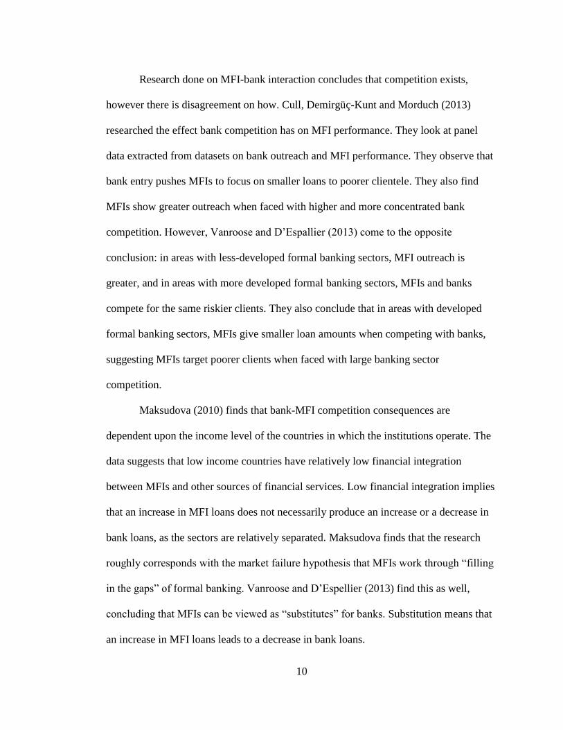
Research done on MFI-bank interaction concludes that competition exists,
however there is disagreement on how. Cull, Demirgüç-Kunt and Morduch (2013)
researched the effect bank competition has on MFI performance. They look at panel
data extracted from datasets on bank outreach and MFI performance. They observe that
bank entry pushes MFIs to focus on smaller loans to poorer clientele. They also find
MFIs show greater outreach when faced with higher and more concentrated bank
competition. However, Vanroose and D’Espallier (2013) come to the opposite
conclusion: in areas with less-developed formal banking sectors, MFI outreach is
greater, and in areas with more developed formal banking sectors, MFIs and banks
compete for the same riskier clients. They also conclude that in areas with developed
formal banking sectors, MFIs give smaller loan amounts when competing with banks,
suggesting MFIs target poorer clients when faced with large banking sector
competition.
Maksudova (2010) finds that bank-MFI competition consequences are
dependent upon the income level of the countries in which the institutions operate. The
data suggests that low income countries have relatively low financial integration
between MFIs and other sources of financial services. Low financial integration implies
that an increase in MFI loans does not necessarily produce an increase or a decrease in
bank loans, as the sectors are relatively separated. Maksudova finds that the research
roughly corresponds with the market failure hypothesis that MFIs work through “filling
in the gaps” of formal banking. Vanroose and D’Espellier (2013) find this as well,
concluding that MFIs can be viewed as “substitutes” for banks. Substitution means that
an increase in MFI loans leads to a decrease in bank loans.

11
Cull, Demirgüç-Kunt and Morduch (2013) also conclude that MFIs that are
commercially funded, offer individual instead of joint liability loans, or take deposits
will be more greatly affected by competition than other types of MFIs. Vanroose and
D’Espallier (2013) also find institutional characteristics such as age, size, and legal
status of the MFI influence MFI-bank competition.
Cull, Demirgüç-Kunt and Morduch (2013) do not find that bank competition
negatively affects overall MFI financial performance, however they conclude that
financial performance for MFIs with urban clientele that geographically overlap with
bank branches is negatively affected. They hypothesize that MFIs cannot adequately use
the incentive of future loan denial when there is stronger bank presence, or that MFIs
may simply not be able to compete with larger banks when it comes to the services
provided and the prices charged.
The research shows that competition consequences are present on an aggregated
scale. Differences in country income, MFI institutional characteristics, and level of
formal banking sector development all contribute to level of competition between banks
and MFIs. The literature suggests competition exists between the two sectors, which
would imply that competition would be present in my study. However, the competition
being picked up in these studies is on a more aggregated scale than that of the data with
which I work, so even though competition is seen on a larger, cross-country and cross-
institutional scale, it is not necessarily true that finding no competition in this study
would produce a contradictory result to what others have found.
12
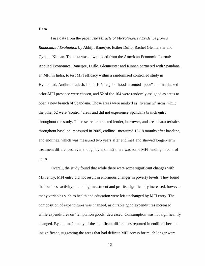
Data
I use data from the paper The Miracle of Microfinance? Evidence from a
Randomized Evaluation by Abhijit Banerjee, Esther Duflo, Rachel Glennerster and
Cynthia Kinnan. The data was downloaded from the American Economic Journal:
Applied Economics. Banerjee, Duflo, Glennerster and Kinnan partnered with Spandana,
an MFI in India, to test MFI efficacy within a randomized controlled study in
Hyderabad, Andhra Pradesh, India. 104 neighborhoods deemed “poor” and that lacked
prior-MFI presence were chosen, and 52 of the 104 were randomly assigned as areas to
open a new branch of Spandana. Those areas were marked as ‘treatment’ areas, while
the other 52 were ‘control’ areas and did not experience Spandana branch entry
throughout the study. The researchers tracked lender, borrower, and area characteristics
throughout baseline, measured in 2005, endline1 measured 15-18 months after baseline,
and endline2, which was measured two years after endline1 and showed longer-term
treatment differences, even though by endline2 there was some MFI lending in control
areas.
Overall, the study found that while there were some significant changes with
MFI entry, MFI entry did not result in enormous changes in poverty levels. They found
that business activity, including investment and profits, significantly increased, however
many variables such as health and education were left unchanged by MFI entry. The
composition of expenditures was changed, as durable good expenditures increased
while expenditures on ‘temptation goods’ decreased. Consumption was not significantly
changed. By endline2, many of the significant differences reported in endline1 became
insignificant, suggesting the areas that had definite MFI access for much longer were
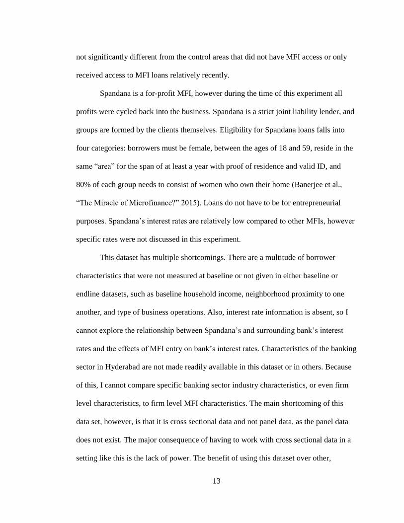
13
not significantly different from the control areas that did not have MFI access or only
received access to MFI loans relatively recently.
Spandana is a for-profit MFI, however during the time of this experiment all
profits were cycled back into the business. Spandana is a strict joint liability lender, and
groups are formed by the clients themselves. Eligibility for Spandana loans falls into
four categories: borrowers must be female, between the ages of 18 and 59, reside in the
same “area” for the span of at least a year with proof of residence and valid ID, and
80% of each group needs to consist of women who own their home (Banerjee et al.,
“The Miracle of Microfinance?” 2015). Loans do not have to be for entrepreneurial
purposes. Spandana’s interest rates are relatively low compared to other MFIs, however
specific rates were not discussed in this experiment.
This dataset has multiple shortcomings. There are a multitude of borrower
characteristics that were not measured at baseline or not given in either baseline or
endline datasets, such as baseline household income, neighborhood proximity to one
another, and type of business operations. Also, interest rate information is absent, so I
cannot explore the relationship between Spandana’s and surrounding bank’s interest
rates and the effects of MFI entry on bank’s interest rates. Characteristics of the banking
sector in Hyderabad are not made readily available in this dataset or in others. Because
of this, I cannot compare specific banking sector industry characteristics, or even firm
level characteristics, to firm level MFI characteristics. The main shortcoming of this
data set, however, is that it is cross sectional data and not panel data, as the panel data
does not exist. The major consequence of having to work with cross sectional data in a
setting like this is the lack of power. The benefit of using this dataset over other,

14
aggregated panel datasets is that the experiment was set up in such a way that allows for
MFI-entry to be examined exogenously instead of the general endogeneity of entry
variables, therefore ensuring unbiased estimates.
Table 1 shows how loan likelihood and loan amount for banks, MFIs, the
informal credit sector, and all loans change across baseline, endline1, and endline2. All
amounts are in rupees, while the loan likelihoods are in percentage points.
Table 1: Dependent Variable Means Across Measurement Periods
VARIABLES Baseline Endline1 Endline2
Bank 0.0387 0.0816 0.0736
(0.193) (0.274) (0.261)
Bank Amount 4694.693 8755.339 5683.892
(115873.4) (83107.43) (35692.4)
MFI 0.0157 0.2374 0.3409
(0.124) (0.426) (0.474)
MFI Amount 303.8724 3204.176 6136.486
(4580.333) (7414.078) (12547.23)
Informal 0.6278 0.7337 0.6032
(0.483) (0.442) (0.489)
Informal Amount 27075.4 40725.36 32452.63
(64573.6) (86804.74) (80551.54)
Any Loan 0.6762 0.8576 0.9052
(0.468) (0.349) (0.293)
Any Loan Amount 33701.57 62062.73 90927.75
(137417.9) (173419.8) (149981.7)
15
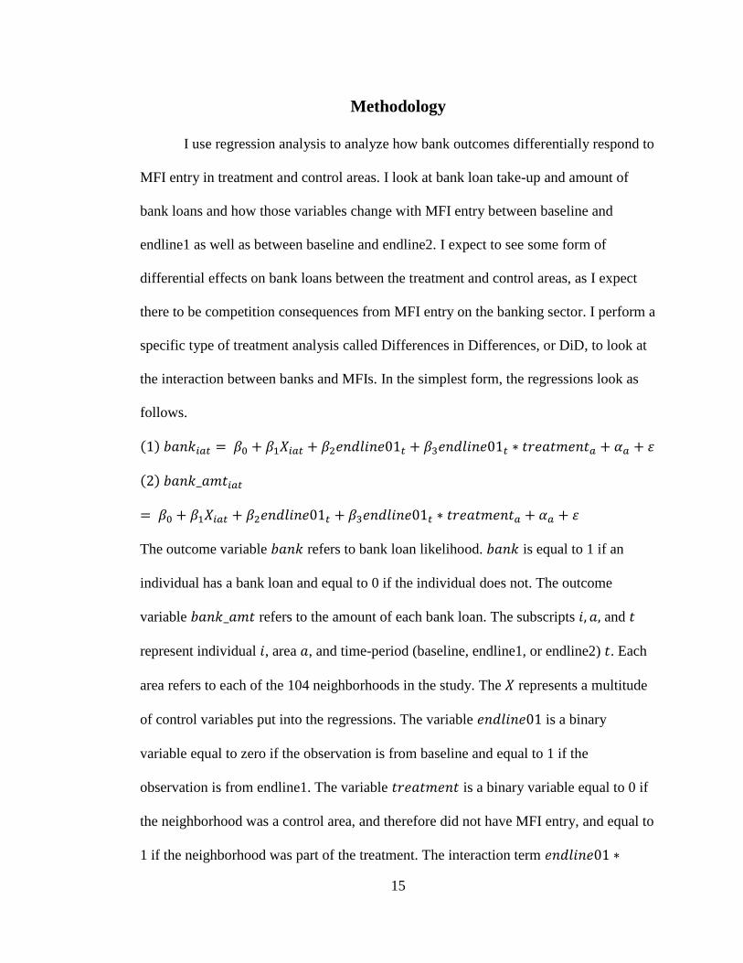
Methodology
I use regression analysis to analyze how bank outcomes differentially respond to
MFI entry in treatment and control areas. I look at bank loan take-up and amount of
bank loans and how those variables change with MFI entry between baseline and
endline1 as well as between baseline and endline2. I expect to see some form of
differential effects on bank loans between the treatment and control areas, as I expect
there to be competition consequences from MFI entry on the banking sector. I perform a
specific type of treatment analysis called Differences in Differences, or DiD, to look at
the interaction between banks and MFIs. In the simplest form, the regressions look as
follows.
(1) 𝑏𝑎𝑛𝑘𝑖𝑎𝑡 = 𝛽0 + 𝛽1𝑋𝑖𝑎𝑡 + 𝛽2𝑒𝑛𝑑𝑙𝑖𝑛𝑒01𝑡 + 𝛽3𝑒𝑛𝑑𝑙𝑖𝑛𝑒01𝑡 ∗ 𝑡𝑟𝑒𝑎𝑡𝑚𝑒𝑛𝑡𝑎 + 𝛼𝑎 + 𝜀
(2) 𝑏𝑎𝑛𝑘_𝑎𝑚𝑡𝑖𝑎𝑡
= 𝛽0 + 𝛽1𝑋𝑖𝑎𝑡 + 𝛽2𝑒𝑛𝑑𝑙𝑖𝑛𝑒01𝑡 + 𝛽3𝑒𝑛𝑑𝑙𝑖𝑛𝑒01𝑡 ∗ 𝑡𝑟𝑒𝑎𝑡𝑚𝑒𝑛𝑡𝑎 + 𝛼𝑎 + 𝜀
The outcome variable 𝑏𝑎𝑛𝑘 refers to bank loan likelihood. 𝑏𝑎𝑛𝑘 is equal to 1 if an
individual has a bank loan and equal to 0 if the individual does not. The outcome
variable 𝑏𝑎𝑛𝑘_𝑎𝑚𝑡 refers to the amount of each bank loan. The subscripts 𝑖, 𝑎, and 𝑡
represent individual 𝑖, area 𝑎, and time-period (baseline, endline1, or endline2) 𝑡. Each
area refers to each of the 104 neighborhoods in the study. The 𝑋 represents a multitude
of control variables put into the regressions. The variable 𝑒𝑛𝑑𝑙𝑖𝑛𝑒01 is a binary
variable equal to zero if the observation is from baseline and equal to 1 if the
observation is from endline1. The variable 𝑡𝑟𝑒𝑎𝑡𝑚𝑒𝑛𝑡 is a binary variable equal to 0 if
the neighborhood was a control area, and therefore did not have MFI entry, and equal to
1 if the neighborhood was part of the treatment. The interaction term 𝑒𝑛𝑑𝑙𝑖𝑛𝑒01 ∗

16
𝑡𝑟𝑒𝑎𝑡𝑚𝑒𝑛𝑡 reflects the differences from baseline to endline1 between treatment and
control areas. The coefficient associated with this interaction term, 𝛽3, is my DiD
estimator and my main coefficient of interest in both regressions. I include area fixed
effects in each regression, 𝛼, to account for area-level differences. I then perform these
same regressions, replacing 𝑒𝑛𝑑𝑙𝑖𝑛𝑒01 with 𝑒𝑛𝑑𝑙𝑖𝑛𝑒02, a binary variable equal to zero
if the observation is from baseline and equal to 1 if the observation is from endline2, to
look at longer-run differences from baseline to endline2 and compare the direction and
magnitude of the effects experienced at endline1.
It is possible that a bank’s decision to compete with an MFI is dependent upon
area-level characteristics. This would mean that treatment areas with high values of
certain area-specific characteristics would have differential bank outcomes as compared
to control areas. For example, banks could be competing with MFIs in high literacy
areas but not competing in low literacy ones. To examine this, I use five area-specific
variables, or value indicators, measured at baseline – previous banking in the area, total
area expenditures, total area debt, total number of businesses in the area, and area
literacy rate. I use these five as they were all measured at baseline and theoretically
would contribute to the credit worthiness of each area.
I create two distinct binary variables for each value indicator and in turn perform
triple difference analyses on each of the binary variables. This is to say I look at the
differences from baseline to endline1 or endline2, between treatment and control areas,
between areas above or below the value indicator of interest. I create two binaries for
each value indicator so I can examine robustness of findings. Areas at or above cutoffs

17
are deemed “high value” areas. Table 2 shows the distinct cutoffs for each value
indicator.
Table 2: Value Indicator Variable Cutoffs
Value Indicator Cutoff Value
Already Banked 1 1
2 2
Expenditures 50% 998.3371
75% 1095.726
Debt 50% 34122.68
75% 38675
Businesses 50% 7.24966
75% 11
Literacy 50% 0.6823932
75% 0.7478261
All value indicators besides debt are designed as follows: if the area value indicator is
at or above the cutoff, then the value indicator is equal to 1. Otherwise, it is equal to 0.
Debt is set up in the opposite way – if area debt is below the cutoff, debt is equal to 1.
Otherwise, it is equal to 0. A ‘high value debt area’ still refers to an area with average
total debt above the cutoff.
The first value indicator is 𝑎𝑙𝑟𝑒𝑎𝑑𝑦_𝑏𝑎𝑛𝑘𝑒𝑑 which indicates if an area had banking
sector presence at baseline. I use previous banking to proxy for financial sector
integration that Cull et al. (2013) and Vanroose and D’Espallier (2013) found to be a
determinant for competition. I say that if someone in the area has an outstanding bank
loan at baseline then the area is already banked. The second cutoff is if at least two
people in an area have an outstanding bank loan at baseline. This is a practical proxy for
previous banking as long as borrowers obtain financing from branches or lenders in
their own neighborhoods. The other four value indicators have cutoffs based on the
mean and upper quartile values. The value indicator 𝑒𝑥𝑝𝑒𝑛𝑑 is the area monthly
expenditures at baseline, which I use as a proxy for income. The value indicator 𝑑𝑒𝑏𝑡 is
the area’s total debt at baseline. The value indicator 𝑏𝑖𝑧 is the total number of

18
businesses in an area at baseline. The value indicator 𝑙𝑖𝑡 is the literacy rate of each area
at baseline.
I run four main regressions for each threshold, and then repeat the regressions
replacing 𝑒𝑛𝑑𝑙𝑖𝑛𝑒01 with 𝑒𝑛𝑑𝑙𝑖𝑛𝑒02 and replacing 𝑏𝑎𝑛𝑘 with 𝑏𝑎𝑛𝑘_𝑎𝑚𝑡. The
regressions look as follows:
(3) 𝑏𝑎𝑛𝑘𝑖𝑎𝑡
= 𝛽0 + 𝛽1𝑋𝑖𝑎𝑡 + 𝛽2𝑒𝑛𝑑𝑙𝑖𝑛𝑒01𝑡 + 𝛽3𝑒𝑛𝑑𝑙𝑖𝑛𝑒01𝑡 ∗ ℎ𝑖𝑔ℎ_𝑣𝑎𝑙𝑢𝑒𝑎 + 𝛼𝑎 + 𝜀
(4) 𝑏𝑎𝑛𝑘𝑖𝑎𝑡
= 𝛽0 + 𝛽1𝑋𝑖𝑎𝑡 + 𝛽2𝑒𝑛𝑑𝑙𝑖𝑛𝑒01𝑡 + 𝛽3𝑒𝑛𝑑𝑙𝑖𝑛𝑒01𝑡 ∗ 𝑡𝑟𝑒𝑎𝑡𝑚𝑒𝑛𝑡𝑎 + 𝛽4𝑒𝑛𝑑𝑙𝑖𝑛𝑒01𝑡
∗ ℎ𝑖𝑔ℎ_𝑣𝑎𝑙𝑢𝑒𝑎 + 𝛽5𝑡𝑟𝑒𝑎𝑡𝑚𝑒𝑛𝑡𝑎 ∗ ℎ𝑖𝑔ℎ_𝑣𝑎𝑙𝑢𝑒𝑎 + 𝛽6𝑒𝑛𝑑𝑙𝑖𝑛𝑒01𝑡 ∗ ℎ𝑖𝑔ℎ_𝑣𝑎𝑙𝑢𝑒𝑎
∗ 𝑡𝑟𝑒𝑎𝑡𝑚𝑒𝑛𝑡𝑎 + 𝛼𝑎 + 𝜀
(5) 𝑏𝑎𝑛𝑘𝑖𝑎𝑡
= 𝛽0 + 𝛽1𝑋𝑖𝑎𝑡 + 𝛽2𝑒𝑛𝑑𝑙𝑖𝑛𝑒01𝑡 + 𝛽3𝑒𝑛𝑑𝑙𝑖𝑛𝑒01𝑡 ∗ ℎ𝑖𝑔ℎ_𝑣𝑎𝑙𝑢𝑒𝑎 + 𝛼𝑎
+ 𝜀 𝑖𝑓 𝑡𝑟𝑒𝑎𝑡𝑚𝑒𝑛𝑡 = 1
(6) 𝑏𝑎𝑛𝑘𝑖𝑎𝑡
= 𝛽0 + 𝛽1𝑋𝑖𝑎𝑡 + 𝛽2𝑒𝑛𝑑𝑙𝑖𝑛𝑒01𝑡 + 𝛽3𝑒𝑛𝑑𝑙𝑖𝑛𝑒01𝑡 ∗ ℎ𝑖𝑔ℎ_𝑣𝑎𝑙𝑢𝑒𝑎 + 𝛼𝑎
+ 𝜀 𝑖𝑓 𝑡𝑟𝑒𝑎𝑡𝑚𝑒𝑛𝑡 = 0
The ℎ𝑖𝑔ℎ_𝑣𝑎𝑙𝑢𝑒 variable is a place holder for each of the ten value indicators described
above (five types, two cutoffs per type). Regression (3) allows me to look at differences
in banking across endlines between high and low value areas to see if and how the
banking sector is dependent on each area characteristic. Regression (4) is the triple
difference regression, which shows differences between treatment and control areas
across endlines, dependent on different value indicators. This tells me if the banking

19
sector’s response to MFI entry differs for high and low value areas. Regressions (5) and
(6) show how banking responds to these different value indicators within treatment and
control areas separately. There are multiple cases where the triple difference regression
coefficients are insignificant but there are significant coefficients within one or both of
the treatment and control samples.
By looking at differences across both baseline to endline1 and baseline to
endline2 I can see the robustness of the results across time and look to see what effects,
if any, are being picked up only in the short run or only in the long run. I also look at
the robustness of the results by using two different cutoffs, the second of which would
be assumed to be a stricter cut as less areas are considered high value.
To gain a complete picture of the effects of the interaction, I look at similar
outcomes in both the MFI sector and the informal credit sector, specifically looking at
differences in treatment and control areas with respect to the value indicators. I examine
the two treatment effect regressions, (1) and (2), while replacing the dependent
variables with 𝑚𝑓𝑖, 𝑚𝑓𝑖_𝑎𝑚𝑡, 𝑖𝑛𝑓𝑜𝑟𝑚𝑎𝑙, and 𝑖𝑛𝑓𝑜𝑟𝑚𝑎𝑙_𝑎𝑚𝑡. I then replace
𝑒𝑛𝑑𝑙𝑖𝑛𝑒01 with 𝑒𝑛𝑑𝑙𝑖𝑛𝑒02 to look at long term effects. To conclude these sector
analyses, I run regressions (4) (5) and (6) with the new dependent variables, however I
only use the first cutoff of each value indicator and I only look across endline1 as
robustness in these sectors is not the focus of this study. The purposes of looking at the
informal sector and the MFI sector are to see how the outcomes of those sectors
compare to the outcomes of the banking sector and, more importantly, to use these
analyses to examine possible theories as to why banking behavior responds to MFI
entry the way it does.

20
Finally, I examine characteristics that determine bank and MFI loan take-up to
look at differences in clientele. This analysis shows how separate the markets are for
banks and MFIs. All characteristic analysis is done only on endline1 and endline2 as
baseline data on the individual level cannot be matched with endline data on the
individual level. I also run the same characteristics through a regression only on the
dependent variable 𝑏𝑎𝑛𝑘, using only the sample of people that borrow from either an
MFI or a bank. Any statistically significant coefficients produced from this regression
are statistical differences between clientele characteristics for banks and for MFIs.
I then build a table of means that displays what the average value is for each
clientele characteristic when the borrower has borrowed from a bank and the borrower
has borrowed from an MFI. In this table, I present t-statistics that show if there are
statistically significant differences between the average values for both samples. This
shows me whether each characteristic is significantly different between bank and MFI
clientele, and allows me to conclude whether bank and MFI clientele are statistically
different from one another. This analysis allows me to hypothesize more directly as to
whether banks and MFIs operate in significantly different marketspaces.
Variables on the household level are household size, whether the head of the
household is male, the age of the head, whether the head has education, whether the
household owned a business at least one year before endline1, and whether the
household owns land. Area specific variables taken into consideration are area
populations at baseline, whether an area has high or low business activity at baseline,
whether an area has high or low expenditures at baseline, whether an area has a high or
low literacy rate at baseline, and whether an area had previous banking at baseline. All

21
area variables that are used here that were used above are based on the mean variable
threshold. Lastly, indexes used in the original study on women employment, income,
labor, consumption, and social factors are taken into consideration.
22
Results
Banking Sector
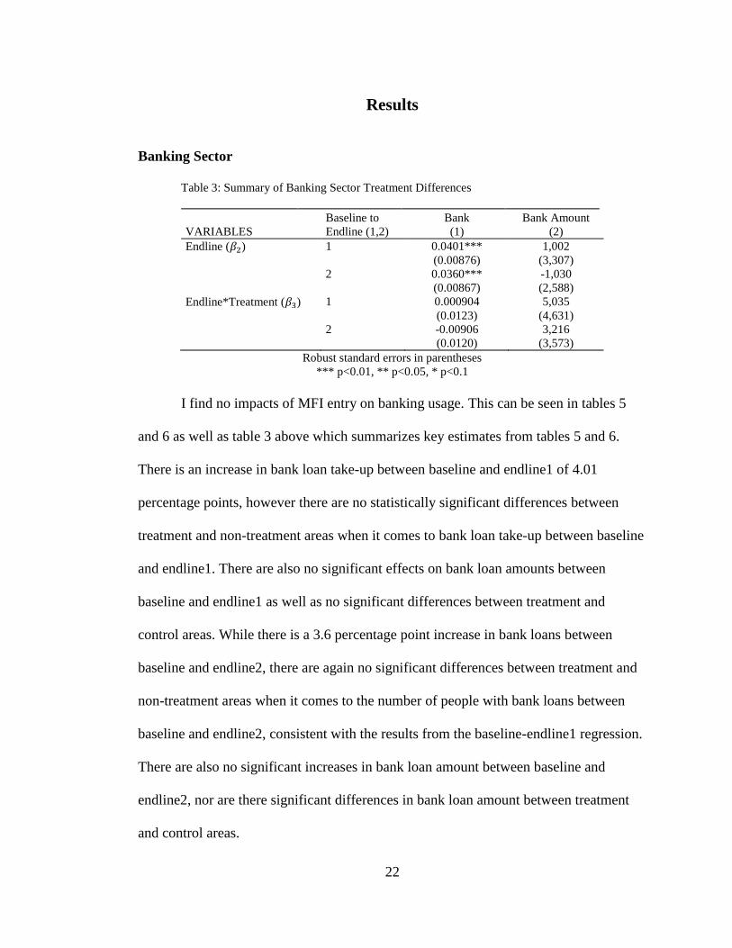
Table 3: Summary of Banking Sector Treatment Differences
VARIABLES
Baseline to
Endline (1,2)
Bank
(1)
Bank Amount
(2)
Endline (𝛽2) 1 0.0401*** 1,002
(0.00876) (3,307)
2 0.0360*** -1,030
(0.00867) (2,588)
Endline*Treatment (𝛽3) 1 0.000904 5,035
(0.0123) (4,631)
2 -0.00906 3,216
(0.0120) (3,573)
Robust standard errors in parentheses
*** p<0.01, ** p<0.05, * p<0.1
I find no impacts of MFI entry on banking usage. This can be seen in tables 5
and 6 as well as table 3 above which summarizes key estimates from tables 5 and 6.
There is an increase in bank loan take-up between baseline and endline1 of 4.01
percentage points, however there are no statistically significant differences between
treatment and non-treatment areas when it comes to bank loan take-up between baseline
and endline1. There are also no significant effects on bank loan amounts between
baseline and endline1 as well as no significant differences between treatment and
control areas. While there is a 3.6 percentage point increase in bank loans between
baseline and endline2, there are again no significant differences between treatment and
non-treatment areas when it comes to the number of people with bank loans between
baseline and endline2, consistent with the results from the baseline-endline1 regression.
There are also no significant increases in bank loan amount between baseline and
endline2, nor are there significant differences in bank loan amount between treatment
and control areas.
23
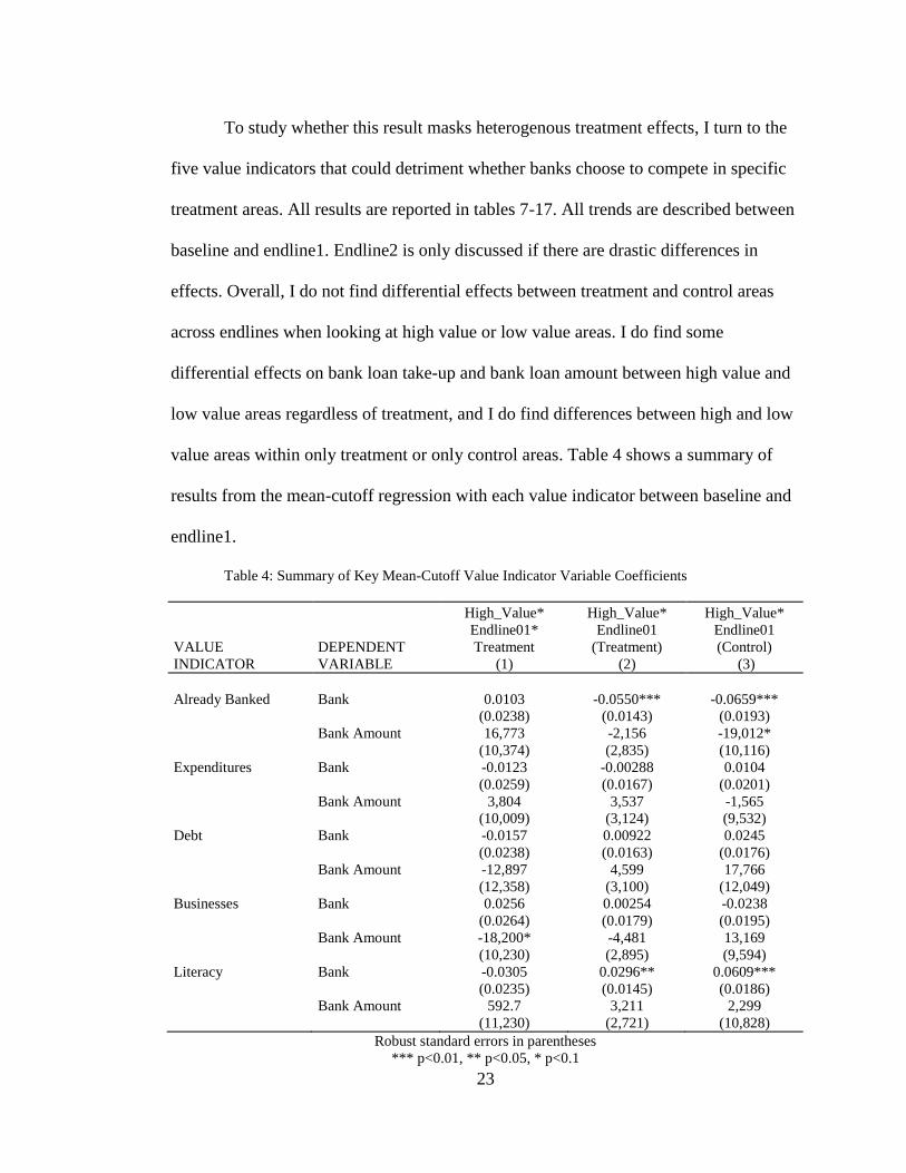
To study whether this result masks heterogenous treatment effects, I turn to the
five value indicators that could detriment whether banks choose to compete in specific
treatment areas. All results are reported in tables 7-17. All trends are described between
baseline and endline1. Endline2 is only discussed if there are drastic differences in
effects. Overall, I do not find differential effects between treatment and control areas
across endlines when looking at high value or low value areas. I do find some
differential effects on bank loan take-up and bank loan amount between high value and
low value areas regardless of treatment, and I do find differences between high and low
value areas within only treatment or only control areas. Table 4 shows a summary of
results from the mean-cutoff regression with each value indicator between baseline and
endline1.
Table 4: Summary of Key Mean-Cutoff Value Indicator Variable Coefficients
VALUE
INDICATOR
DEPENDENT
VARIABLE
High_Value*
Endline01*
Treatment
(1)
High_Value*
Endline01
(Treatment)
(2)
High_Value*
Endline01
(Control)
(3)
Already Banked Bank 0.0103 -0.0550*** -0.0659***
(0.0238) (0.0143) (0.0193)
Bank Amount 16,773 -2,156 -19,012*
(10,374) (2,835) (10,116)
Expenditures Bank -0.0123 -0.00288 0.0104
(0.0259) (0.0167) (0.0201)
Bank Amount 3,804 3,537 -1,565
(10,009) (3,124) (9,532)
Debt Bank -0.0157 0.00922 0.0245
(0.0238) (0.0163) (0.0176)
Bank Amount -12,897 4,599 17,766
(12,358) (3,100) (12,049)
Businesses Bank 0.0256 0.00254 -0.0238
(0.0264) (0.0179) (0.0195)
Bank Amount -18,200* -4,481 13,169
(10,230) (2,895) (9,594)
Literacy Bank -0.0305 0.0296** 0.0609***
(0.0235) (0.0145) (0.0186)
Bank Amount 592.7 3,211 2,299
(11,230) (2,721) (10,828)
Robust standard errors in parentheses
*** p<0.01, ** p<0.05, * p<0.1

24
Previous Banking
Borrowing in previously unbanked areas, i.e. areas with at least one person who
had an outstanding bank loan at baseline, appears to play catch-up to and sometimes
surpass borrowing in previously banked areas. All results for the already banked
indicator are reported in tables 7 and 8. Areas that were banked at baseline are slightly
more likely to have a bank loan at endline1 than baseline, but are 5.99 percentage points
less likely to have a bank loan at endline1 than those in previously unbanked areas,
significant at the 1% level. Using the second cutoff of already banked, i.e. at least two
people who had outstanding bank loans at baseline, the likelihood that people in
previously banked areas have a bank loan decreases between baseline and endline1 by
0.17 percentage. The difference in bank loan take-up at endline1 between previously
banked and unbanked areas is similar to yet slightly smaller than that of the first cutoff.
While there are differences between previously banked and unbanked areas,
there are no significant differential effects of previous banking on bank loans between
treatment and control areas. Within treatment areas, people in already banked areas are
5.50 percentage points less likely to have a bank loan at endline1 than people in
previously unbanked areas. Within control areas, people in areas that were previously
banked are 6.59 percentage points less likely to have an outstanding bank loan at
endline1 than people in areas that were previously unbanked. All results are significant
at the 1% level. The second cutoff produces similar results, with the difference in bank
loan take-up within treatment areas becoming slightly larger while said difference
within control areas becomes slightly smaller and is significant at the 5% level.
Although there are significant differences within treatment and within control areas, the

25
effects are of similar direction and magnitude which explains the insignificant
coefficients in the triple interaction.
There are significant effects on bank loan amounts. People in already banked
areas see a decline in average bank loan amounts between baseline and endline1 by a
factor of 10,610 Rs. in comparison to areas that were previously unbanked, significant
at the 5% level. This difference is so large that people in previously banked areas see a
decrease in bank loan amount while people in previously unbanked areas experience an
increase between baseline and endline1. Using the second cutoff, this effect becomes
insignificant.
There are no significant effects on bank loan amount for the triple interaction
nor within treatment areas. Within control areas, people in previously banked areas have
smaller bank loan amounts than their previously unbanked counterparts by 19012 Rs. at
endline1, significant at the 10% level. Again, this difference is large enough that people
in control and previously banked areas experience a decline in bank loan amounts
between baseline and endline1 while those in control and previously unbanked areas
experience an increase. Effects become insignificant at endline2 when using the second
cutoff.
Business Activity
All results for the business indicator are in tables 9 and 10. High value business
areas have no significant differential effects on bank loan take-up across endlines,
regardless of cutoff. There are also no significant differential effects between treatment
and control areas, nor are there significant effects within either sample of treatment
areas or control areas.
26
There are significant effects on bank loan amounts. The triple interaction
regression concerning treatment, endlines, and high value business areas is significant.
For high value business areas, treatment areas have on average bank loans that are
18200.06 Rs. less than those in control areas at endline1, using the first business cutoff.
The second cutoff produces a slightly larger difference. Both of these results are
significant at the 10% level. This result becomes insignificant when looking at endline2.
Using the second business cutoff, there are significant estimates within the
treatment sample. People in high value business treatment areas have smaller bank
loans at endline1 by 6015 Rs. than those in low value business treatment areas,
significant at the 10% level. There are no significant estimates for treatment areas using
the first cutoff nor are there significant estimates for control areas.
Debt
All results for the debt indicator are in tables 11 and 12. There are no significant
differential effects of either debt variable on bank loan take-up across baseline and
endline1. There are no significant effects of high value debt areas on bank loan take-up
between treatment and control areas across endlines, nor are there significant
differences in bank loan take-up within the treatment sample nor within the control
sample.
There are no significant differential effects of high value debt areas on bank loan
amounts between treatment and control areas. There are no significant effects within
control areas nor within treatment areas at endline1. However, there are some
significant estimates. People in low value debt areas on average have bank loan
amounts at endline1 that are 11479 Rs. larger than those in high value debt areas,
27
significant at the 10% level when using the first debt cutoff. This result is insignificant
when looking at endline2 or when using the second debt cutoff. However, using both
debt cutoffs at endline2, low value debt treatment areas are shown to have larger bank
loan amounts than high value debt treatment areas, significant at the 10% level. The
second cutoff produces a slightly larger difference than the first.
Expenditures
All results for the expenditure indicator are reported in tables 13 and 14. I find
no significant differences in bank loan take-up or bank loan amount between high and
low value expenditure areas. There are no significant differential effects of high value
expenditure areas between treatment and control areas. There are also no differential
effects of high and low expenditures on bank loan take-up or bank loan amount within
treatment areas nor within control areas. These trends are true for both cutoffs.
Literacy Rates
All results for the literacy indicator are in tables 15 and 16. People in high value
literacy areas are 4.49 percentage points more likely to have a bank loan at endline1
than those in low value literacy areas, using the first cutoff. The triple interaction term
is not significant between baseline and endline1. However, between baseline and
endline2 the triple difference estimate is significant for both literacy cutoffs. At endline
2, high value literacy treatment areas are 4.13 or 5.38 percentage points less likely to
have a bank loan relative to high value literacy control areas, respective to each cutoff.
The first cutoff is significant at the 10% level while the second cutoff is significant at
5%.

28
Those in high value literacy treatment areas are 2.96 percentage points more
likely to have a bank loan at endline1 than those in low value literacy treatment areas,
significant at the 5% level, using only the first cutoff. Those in high value literacy
control areas are 6.09 percentage points more likely to have a bank loan than those in
low value literacy control areas at endline1, significant at the 1% level. The second
literacy cutoff produces a similar yet slightly smaller difference. There are no
significant effects of high value literacy areas on bank loan amounts, nor are there
significant differential effects of literacy on bank loan amounts between treatment and
control areas nor within either sample of treatment or control areas.
Informal and MFI sectors
I examine informal loans and MFI loans to get a sense of how treatment affected
these types of loans and to compare effects against bank loans. As neither informal
sector effects nor MFI sector effects are the focus of this study, I do not check effects as
extensively as with the banking sector. I do not show the results against endline2 or
against the second cutoff for each value indicator. Only the triple difference coefficients
are reported in the tables, however I do explain some within-sample trends that, while
not affecting the banking sector, are interesting to note.
Informal
Tables 18 and 19 show results for the informal credit sector. There are
significant increases in informal loan take-up and informal loan amount between
baseline and endline1. There is a significant decrease in informal loan take-up at
endline2, while the estimate for bank loan amount at endline2 is insignificant. There are

29
no significant differences between treatment and control areas when it comes to
informal loan take-up and informal loan amounts between baseline and endline1. There
also exist no significant differences between treatment and control areas when it comes
to previous banking, high value expenditure areas, high value business areas, high value
debt areas, or high value literacy areas. There are also no significant differences within
treatment areas nor within control areas when it comes to previously banking, high
value expenditure areas, or high value literacy areas.
In treatment areas, people in high value business areas experience smaller
amounts of informal loans as compared to their low value business area counterparts at
endline1. This effect is insignificant in control areas. There is also no significant effect
on informal loan take-up in neither treatment nor control areas with respect to high
value business areas.
People in low value debt control areas have a higher likelihood of having an
informal loan at endline1 as compared to their high value debt control area counterparts.
There is no such significant difference for treatment areas. People in low value debt
areas experience significantly larger informal loans than those in high value debt areas
at endline1 in both samples of treatment and control areas.
MFI
Tables 20 and 21 show results for the MFI sector. There are significant positive
effects on the number of people with MFI loans between baseline and endline1 as well
as the amount of those MFI loans. There are positive differential effects between
treatment and control areas, as treatment areas have much higher loan take-up and loan
amounts. All effects become insignificant at endline2.

30
There are no significant differential effects for either MFI loan take-up or
amount between treatment and control areas when it comes to previous banking, high
value expenditure areas, high value business areas, or high value literacy areas. There
are also no significant differences in loan take-up or loan amount within treatment nor
within control areas between previously banked or unbanked areas, high or low
expenditure areas, or high or low literacy areas. High value business areas are 8.19
percentage points less likely to have MFI loans than those in low value business areas at
endline1. No such significant effects appear in control areas, nor when it comes to bank
loan amount.
The only significant triple interactions come from the debt variable. People in
low value debt treatment areas are 12.03 percentage points more likely to have an MFI
loan than those in low value debt control areas. People in low value debt treatment areas
also experience larger MFI loan amounts than those in low value debt control areas.
Within treatment areas, people in low value debt areas are 11.95 percentage points more
likely to have an MFI loan than those in high value debt areas. They also have higher
loan amounts than those in high value debt areas. All estimates for control areas are
insignificant.
Characteristics of MFI and Bank loan take-up
I examine whether banks and MFIs loan to individuals based on characteristics
measured in the study. I look at how those characteristics compare to one another in the
two different sectors. I then examine the means of all characteristics for both banks and
MFIs, and test for statistical differences between means. I find there are multiple
characteristics significant in one group and not the other. I also find many statistically
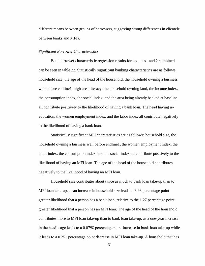
31
different means between groups of borrowers, suggesting strong differences in clientele
between banks and MFIs.
Significant Borrower Characteristics
Both borrower characteristic regression results for endlines1 and 2 combined
can be seen in table 22. Statistically significant banking characteristics are as follows:
household size, the age of the head of the household, the household owning a business
well before endline1, high area literacy, the household owning land, the income index,
the consumption index, the social index, and the area being already banked at baseline
all contribute positively to the likelihood of having a bank loan. The head having no
education, the women employment index, and the labor index all contribute negatively
to the likelihood of having a bank loan.
Statistically significant MFI characteristics are as follows: household size, the
household owning a business well before endline1, the women employment index, the
labor index, the consumption index, and the social index all contribute positively to the
likelihood of having an MFI loan. The age of the head of the household contributes
negatively to the likelihood of having an MFI loan.
Household size contributes about twice as much to bank loan take-up than to
MFI loan take-up, as an increase in household size leads to 3.93 percentage point
greater likelihood that a person has a bank loan, relative to the 1.27 percentage point
greater likelihood that a person has an MFI loan. The age of the head of the household
contributes more to MFI loan take-up than to bank loan take-up, as a one-year increase
in the head’s age leads to a 0.0798 percentage point increase in bank loan take-up while
it leads to a 0.251 percentage point decrease in MFI loan take-up. A household that has

32
an old business at least one year before endline1 is 1.6 percentage points more likely to
have a bank loan, while they are 8.07 percentage points more likely to have an MFI
loan. An increase in the women employment index leads to a decrease in bank loan
take-up by 1.15 percentage points, while it leads to an increase in MFI loan take-up by
3.97 percentage points and is much more significant. The labor index is similar in that
an increase leads to a decrease in bank loan take-up by 1.57 percentage points while it
leads to an increase in MFI loan take-up by 9.81 percentage points. The consumption
index has a positive relation to both bank and MFI loan take-up, with an increase
leading to a 4.7 percentage point increase for the banking sector and a 1.41 percentage
point increase in the MFI sector. The social index also contributes positively to both
sectors’ loan take-up, with a one unit increase leading to a 2.71 percentage point
increase in the banking sector and a 4.23 percentage point increase for MFI loans.
There are changes between endline1 and endline2. Concerning banking
characteristics, the education of the head, owning an old business, literacy rates, and the
social index all become insignificant at endline2 while they are significant at endline1.
Being already banked at baseline is the only significant estimate in endline2 that is not
significant at endline1. Concerning MFI characteristics, having a male head, being
already banked at baseline, and the social index are all significant at endline1 but not
significant at endline2. The consumption index is the only significant estimate for
endline2 that is not significant at endline1.
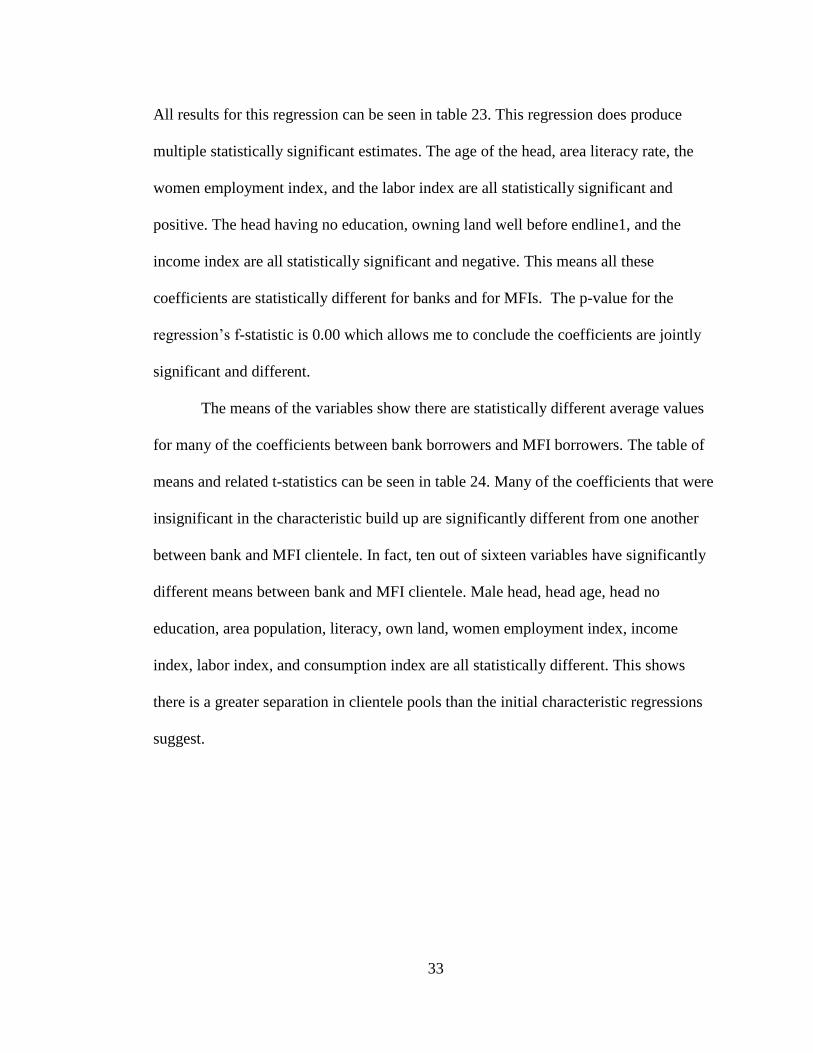
Significant Differences in Borrower Characteristics
I run the same regression on bank likelihood as before, however I restrict the
sample to only people who have outstanding bank or MFI loans at endline1 or endline2.
33
All results for this regression can be seen in table 23. This regression does produce
multiple statistically significant estimates. The age of the head, area literacy rate, the
women employment index, and the labor index are all statistically significant and
positive. The head having no education, owning land well before endline1, and the
income index are all statistically significant and negative. This means all these
coefficients are statistically different for banks and for MFIs. The p-value for the
regression’s f-statistic is 0.00 which allows me to conclude the coefficients are jointly
significant and different.
The means of the variables show there are statistically different average values
for many of the coefficients between bank borrowers and MFI borrowers. The table of
means and related t-statistics can be seen in table 24. Many of the coefficients that were
insignificant in the characteristic build up are significantly different from one another
between bank and MFI clientele. In fact, ten out of sixteen variables have significantly
different means between bank and MFI clientele. Male head, head age, head no
education, area population, literacy, own land, women employment index, income
index, labor index, and consumption index are all statistically different. This shows
there is a greater separation in clientele pools than the initial characteristic regressions
suggest.
34
Discussion
Overall, there is little evidence of any effects of MFI entry on banking
characteristics. The lack of treatment differences in the banking sector shows that
banking characteristics are not affected by MFI competition, as bank loan take-up and
bank loan amounts are not statistically different between treatment and control areas.
Examining the five area-specific value indicator variables – already banked,
expenditures, debt, total businesses, and literacy rates – allows for a more specific
analysis of MFI-bank competition. Banks could be operating differently dependent on
these specific neighborhood characteristics. However, the only statistically significant
difference in bank loan take-up between treatment and control areas is for high value
literacy areas at endline2, significant at both literacy cutoffs. People in high value
literacy treatment areas are less likely on average to have bank loans. The only
statistically significant difference in bank loan amounts between treatment and control
areas is at endline1 with concern to high value business areas, significant at both
business cutoffs. People in high value business treatment areas have on average smaller
bank loans.
If anything, the effects that are statistically significant suggest a possible
substitution effect between MFI loans and bank loans. This substitution effect agrees
with Maksudova (2010) and Vanroose and D’Espallier (2013). Both value indicators
that produce statistically significant triple difference estimates produce negative
coefficients, meaning people in areas with MFI presence are either less likely to borrow
from banks or have smaller bank loan amounts than control area counterparts.

35
Results from the business value indicator suggests that businesses could be
substituting portions of their bank loans with MFI loans, causing areas with many
businesses to have on average bank loan amounts that are less than those in control
areas. Results from the literacy value indicator could suggest that, as literacy and
education level are correlated, borrowers in high literacy areas have more education
surrounding financial services, or are at least more able to educate themselves on
financial services, and in turn find themselves more capable of crossing the barriers to
borrow from new sources. Results could also have to do with differences in lending
type between MFIs and banks. As Spandana is a strict joint liability lender, it could be
that those in higher literacy or higher business activity areas find it more appealing to
pool their risk and operate in a joint liability format.
However, it is important to note the specificity required to achieve these
significant coefficients. Only when combining a specific endline measurement with a
specific value indicator is there a statistically significant result. This only happens in
four out of forty instances tested: both business cutoffs at endline1 on bank loan amount
and both literacy cutoffs at endline2 on bank loan take-up. The lack of robust results
suggests that, while these specific significant differences should not be ignored, an
overall zero effect of MFI competition on banking characteristics is witnessed.
There do exist differences in high value indicator areas that appear within
treatment or within control areas only, however most triple differences are insignificant.
This most likely means the significant effects in one sample are being matched by
similar effects, significant or not, within the other sample. For instance, there are no
significant differences on bank loan take-up between treatment and control areas with
36
respect to previously banked and unbanked areas. However, there are significant
differences between previously banked and unbanked areas within treatment areas as
well as within control areas. In both samples, those in previously banked areas are less
likely to have a bank loan at endline1 than their previously unbanked area counterparts
at endline1. Because this effect is witnessed in both samples, there is no statistically
significant estimate for differences between the two samples. This can also happen
when only one sample has a statistically significant coefficient, as directional similarity
and significance level can contribute to no statistically significant triple difference
estimates. Because differences between treatment and control areas are what are being
tested in this study, differences within samples, while interesting, do not contribute to
whether banks act differently with MFI presence and are not discussed in more depth.
Although differences between treatment and control areas are not witnessed,
there exists a massive increase in lending throughout the period, seen in Table 1. MFI
loan take-up skyrockets due to the nature of the study, with baseline take-up being only
1.57% and endline2 having a take-up of 34.09%. However, both banks and informal
lending institutions experienced increases as well, at least between baseline and
endline1. Bank loan take-up goes from 3.87% at baseline to 8.16% at endline1 to
7.375% at endline2. The informal sector even experiences an increase in loans between
baseline and endline1, as take-up increases from 62.78% to 73.37%, however by
endline2 the take-up rate drops to 60.32%. Overall, the likelihood of anyone having any
type of loan increases from 67.62% to 90.52% between baseline and endline2.
There are a number of possibilities for why there is such an increase. This
increase could by cyclical. Perhaps Hyderabad went through a period of massive
37
lending and much of these increases are uncorrelated with anything concretely
measured. However, these banking and informal increases could be due to a spillover
effect. Even though there does not appear to exist differential effects between treatment
and control areas, it could be that banks are not operating on an area-by-area basis. This
would happen if the banks think of the market differently, outside of the area-based
markets and instead within a much larger market scope than what is measured. This
would mean that much of what is measured here are spillovers from local markets to
one another, and perhaps the area-based definition of a market is too small for the
banking sector.
However, it has been shown in previous research that informal lenders operate
within these smaller, area-based local markets. Because of this type of operation, the
informal sector sheds light on this spillover hypothesis. If it is true that many of these
measurements are spillovers, there would have to exist significant triple difference
coefficients for the informal sector. However, the triple differences are insignificant.
This means that even the informal sector does not experience statistically significant
differences between areas with MFI presence and those without. Therefore, the
spillover theory has no empirical backing, as local markets are not differentially
affected. This again supports a zero effect of MFI entry on the formal banking sector.
While there is a massive increase in lending throughout the study period, the
lack of treatment differences demonstrates the lack of crowding-in effects in the sense
of MFI-bank interactions. If people began financing bank loans with MFI loans, there
would be some differential in bank loan take-up between treatment and control areas, as
treatment areas would supposedly see an increase in bank loans as MFI lending
38
becomes commonplace. The lack of differences reveals the lack of crowding-in effects,
both for bank-MFI sector interactions and for informal-MFI sector interactions.
Clientele characteristics for both banks and MFIs do have some overlap.
Because there is some overlap in characteristics, this would instinctively mean that
there is overlap in clientele. However, there are a multitude of variables that work
against a person’s ability to have a loan in one sector and for their ability in another,
such as head age, women employment index, and labor index. There are also a
multitude of variables that are significant for one sector and not for the other. For
instance, the variable ownland is strongly significant for banks yet insignificant for
MFIs. This represents a characteristic of MFIs which is that they do not require
collateral, so owning land does not matter as much for MFIs as it does for banks. The
income index, lit, and head_no_education are three other variables that are only
significant for banks and could contribute to the idea of why banks and MFIs lend. The
income index and area literacy rates contribute positively to bank loan likelihood while
the head having no education contributes negatively. Increased literacy, education, and
income all signify less risky borrowers. As MFIs operate first and foremost to eradicate
poverty while banks operate primarily as profit-generating institutions, it makes sense
that these variables mean more to a bank than to an MFI.
The regression to explain differences between MFI and bank borrowers
produces some significant coefficients, showing there are significant differences in
clientele between banks and MFIs. Furthermore, the table of means for those
characteristics sheds light on how different these clientele groups really are. Because
there are so many variables that have statistically significant different means, clients are
39
significantly different between banks and MFIs. Although both sectors might act
positively toward a characteristic, such as both MFIs and banks becoming more likely
to lend as the consumption index increases, clientele pools for each sector have
statistically different average values for those characteristics.
The fact that competition is not witnessed between the two industries is baffling,
as I expected to see some competition between two sectors which both lend to
individuals in the same areas. Yet, this zero-effect is the clear conclusion from what is
shown in the difference in difference regressions that produced mostly insignificant
estimates and the statistically different clientele characteristics between the two sectors.
The effects seen in previous papers could be due to endogeneity consequences of their
aggregated panel data, but it also could be that the differences found in those other
papers simply cannot be picked up by this type of dataset. These other studies have
focused on MFI activity surrounding bank presence, whereas I look at bank activity
surrounding MFI presence. While I would still expect to see competition between MFIs
and banks, much of the competition mentioned in previous research would not be
picked up here. For instance, the differences between banking sector development
described by Vanroose and D’Espallier cannot be seen here as this study looks at one
banking sector. Nor can differentials between MFI structures, investigated by Cull,
Demirgüç-Kunt and Morduch, be examined as this study is based off one MFI. The
country level income differences examined by Maksudova also cannot be accounted for
because this data is collected in one city.
While these papers conclude competition effects between the banking sector and
the MFI sector, their conclusion is not necessarily contradictory to mine. My zero-effect

40
conclusion is on the local scale, and none of their results described differential effects
on the local scale. My results add to, rather than contradict, their findings – while there
might exist differences in MFI outreach dependent on banking sector differences, MFI
institutional differences, and income differences across countries, local markets are
relatively separated in MFI lending and bank lending. Because of this market
separation, competitive and non-competitive areas within a city are not differentially
affected. Because this zero effect is witnessed, formal banking sectors in areas where
MFIs operate need not create hostile environments to drive out MFI competition, as
MFIs are seen to not be direct competitors with banks. Instead, banks could work to aid
MFIs in their goal to alleviate poverty, which some larger banks already do. This
finding could also support potential government funding of MFIs as concerns
surrounding negative competition consequences between growing sectors can be
mitigated.
Further research on this topic could cover a multiple of different characteristics.
A more robust dataset, specifically a panel dataset, collected from a controlled study
likened to this one would be extremely beneficial. A more thorough look at bank
clientele, MFI clientele, and informal clientele characteristics could be derived from
such a dataset and used to determine how clientele characteristics shift with MFI entry.
While I attempt to begin this analysis, I cannot perform it thoroughly as all
characteristic data comes from the two endlines and is not tracked over time on an
individual level, only on an area level. Having such a panel would be an excellent
complement to this analysis and would allow for a more intricate look at MFI entry
effects on the banking sector.
41
It would also be interesting to continue a more exhaustive analysis of different
value indicators. This could be done by both expanding the amount of value indicators
collected at the time of the study as well as looking at bank and MFI behavior based
upon these different indicators. One could even move away from bank-MFI competition
and examine the intricacies of how banks and MFIs act dependent on these indicators.
This analysis would ignore treatment versus control to focus on bank and MFI lending
behavior in high versus low value areas. This would contribute to the knowledge pools
of MFI and formal banking determinants and efficacy in the developing world.

42
Conclusion
In this study, I examine differences in banking outcomes in response to MFI
entry. I analyze whether banks compete with MFIs based on certain area characteristics,
or value indicators, or whether the two institutions operate in separate marketplaces. I
do this analysis by running differences in differences and triple difference regressions
that take into consideration differences between measurement periods in the study,
differences between treatment and control areas, and differences between value
indicators that represent area characteristics banks and MFIs could be working off. I
supplement my regression analyses with a clientele characteristic analysis to examine
whether there is overlap in bank and MFI clientele.
I find there exists little to no effect of MFI entry on banking outcomes. There are
no significant estimates of differential treatment effects on bank loan take-up or bank
loan amount. Very few estimates that examine differences from baseline to an endline
between treatment and control areas with respect to differences in area characteristics
come out significant. While these significant exceptions are notable, the overarching
conclusion supports a zero effect estimate of MFI entry on banking sector outcomes.
There is also no support of a spillover hypothesis as the informal sector, a sector known
to operate on an extremely local scale, also experiences no significant triple difference
estimates. This zero-effect finding leads to the conclusion that banks and MFIs are
operating in different marketspaces. This is backed up by the clientele characteristic
analysis. While there does exist some overlap in characteristics, many characteristics
have significantly different means between the two clientele pools, which means banks
and MFIs have statistically different clientele.

43
While there are many conclusions this dataset cannot produce, the brilliance of
this study allows me to thoroughly conclude that exogenous MFI entry does not appear
to affect bank loan take-up or bank loan amounts. While there could be competition
differentials on a larger scale, the lack of competition here shows that bank and MFI
sectors operate in significantly different marketspaces and, on a local scale, interactions
between the sectors do not statistically affect one another’s lending outcomes.

Tables
Table 5: Banking Sector – Treatment Differences from Baseline to Endline1
Bank Bank Amount
VARIABLES (1) (2) (3) (4)
Male Head -0.00237 -141.0
(0.00923) (3,485)
Head Age 0.00101*** 428.7***
(0.000268) (101.2)
Head No
Education
-0.0378*** -9,304***
(0.00607) (2,293)
Household Size 0.00505*** 2,084***
(0.00135) (509.0)
Endline01 0.0459*** 0.0401*** 2,968 1,002
(0.00967) (0.00876) (5,187) (3,307)
Endline01 *
Treatment
0.000325 0.000904 4,823 5,035
(0.0127) (0.0123) (5,399) (4,631)
Constant 0.0359*** -0.0144 3,647* -20,829***
(0.00467) (0.0152) (1,912) (5,738)
Observations 9,242 9,205 9,242 9,205
R-squared 0.036 0.043 0.018 0.024
Robust standard errors in parentheses
*** p<0.01, ** p<0.05, * p<0.1

45
Table 6: Banking Sector – Treatment Differences from Baseline to Endline2
Bank Bank Amount
VARIABLES (1) (2) (3) (4)
Male Head 0.0161** 1,678
(0.00760) (2,269)
Head Age 0.000859*** 211.5***
(0.000267) (79.73)
Head No
Education
-0.0234*** -4,615**
(0.00621) (1,854)
Household Size 0.00109 416.6
(0.00115) (343.1)
Endline02 0.0403*** 0.0360*** 206.9 -1,030
(0.00883) (0.00867) (4,614) (2,588)
Endline02 *
Treatment
-0.00985 -0.00906 3,063 3,216
(0.0111) (0.0120) (4,704) (3,573)
Constant 0.0381*** -0.00792 4,120** -6,369
(0.00392) (0.0141) (1,620) (4,221)
Observations 8,573 8,549 8,573 8,549
R-squared 0.027 0.031 0.019 0.021
Robust standard errors in parentheses
*** p<0.01, ** p<0.05, * p<0.1

46
Table 7: Banking Sector – Effects of Previous Banking Differences between Treatment
and Control from Baseline to Endline1 on Bank Loan take-up
Bank
VARIABLES
(1)
(2)
Treatment
(3)
Control
(4)
Male Head -0.00353 -0.00290 0.0201 -0.0259*
(0.0101) (0.0103) (0.0134) (0.0140)
Head Age 0.00104*** 0.00101*** 0.00106*** 0.000986**
(0.000230) (0.000235) (0.000271) (0.000383)
Head No
Education
-0.0365*** -0.0385*** -0.0356*** -0.0410***
(0.00615) (0.00626) (0.00838) (0.00935)
Household Size 0.00500*** 0.00510*** 0.00519** 0.00501***
(0.00128) (0.00129) (0.00200) (0.00165)
Endline01 0.0748*** 0.0799*** 0.0701*** 0.0796***
(0.00887) (0.0165) (0.00901) (0.0165)
Endline01 *
Treatment
-0.00948
(0.0187)
Endline01 *
Already Banked
-0.0599*** -0.0655*** -0.0550*** -0.0659***
(0.0115) (0.0191) (0.0143) (0.0193)
Endline01 *
Treatment *
Already Banked
0.0103
(0.0238)
Constant -0.0146 -0.0141 -0.0361** 0.00651
(0.0139) (0.0143) (0.0164) (0.0224)
Observations 9,560 9,205 4,757 4,448
R-squared 0.047 0.046 0.041 0.052
Robust standard errors in parentheses
*** p<0.01, ** p<0.05, * p<0.1

47
Table 8: Banking Sector – Effects of Previous Banking Differences between Treatment
and Control from Baseline to Endline1 on Bank Loan Amount
Bank Amount
VARIABLES
(5)
(6)
Treatment
(7)
Control
(8)
Male Head -236.2 -236.4 -411.0 -825.5
(1,515) (1,567) (2,621) (1,656)
Head Age 432.3** 429.7** 93.94 791.5*
(201.0) (209.2) (83.69) (422.4)
Head No
Education
-9,285*** -9,426*** -7,869*** -11,111**
(2,580) (2,667) (1,658) (5,293)
Household Size 2,034*** 2,082*** 1,488* 2,773**
(655.1) (666.2) (790.1) (1,109)
Endline01 9,622*** 12,511* 7,658*** 12,015*
(3,221) (7,106) (1,383) (6,838)
Endline01 *
Treatment
-5,329
(7,466)
Endline01 *
Already Banked
-10,610** -18,933* -2,156 -19,012*
(5,184) (10,028) (2,835) (10,116)
Endline01 *
Treatment *
Already Banked
16,773
(10,374)
Constant -20,559** -20,863** -6,649 -35,822*
(9,889) (10,276) (4,368) (20,401)
Observations 9,560 9,205 4,757 4,448
R-squared 0.025 0.025 0.029 0.027
Robust standard errors in parentheses
*** p<0.01, ** p<0.05, * p<0.1
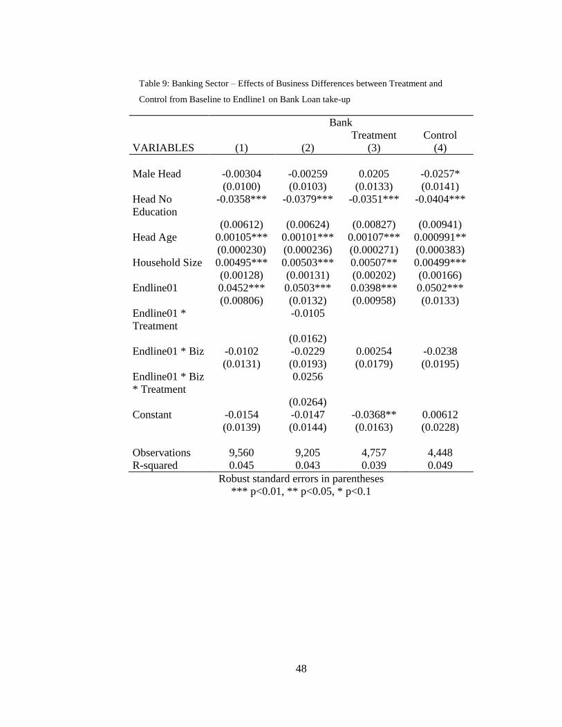
48
Table 9: Banking Sector – Effects of Business Differences between Treatment and
Control from Baseline to Endline1 on Bank Loan take-up
Bank
VARIABLES
(1)
(2)
Treatment
(3)
Control
(4)
Male Head -0.00304 -0.00259 0.0205 -0.0257*
(0.0100) (0.0103) (0.0133) (0.0141)
Head No
Education
-0.0358*** -0.0379*** -0.0351*** -0.0404***
(0.00612) (0.00624) (0.00827) (0.00941)
Head Age 0.00105*** 0.00101*** 0.00107*** 0.000991**
(0.000230) (0.000236) (0.000271) (0.000383)
Household Size 0.00495*** 0.00503*** 0.00507** 0.00499***
(0.00128) (0.00131) (0.00202) (0.00166)
Endline01 0.0452*** 0.0503*** 0.0398*** 0.0502***
(0.00806) (0.0132) (0.00958) (0.0133)
Endline01 *
Treatment
-0.0105
(0.0162)
Endline01 * Biz -0.0102 -0.0229 0.00254 -0.0238
(0.0131) (0.0193) (0.0179) (0.0195)
Endline01 * Biz
* Treatment
0.0256
(0.0264)
Constant -0.0154 -0.0147 -0.0368** 0.00612
(0.0139) (0.0144) (0.0163) (0.0228)
Observations 9,560 9,205 4,757 4,448
R-squared 0.045 0.043 0.039 0.049
Robust standard errors in parentheses
*** p<0.01, ** p<0.05, * p<0.1

49
Table 10: Banking Sector – Effects of Business Differences between Treatment and
Control from Baseline to Endline1 on Bank Loan Amount
Bank Amount
VARIABLES
(5)
(6)
Treatment
(7)
Control
(8)
Male Head -98.07 -4.415 -377.6 -395.4
(1,523) (1,585) (2,624) (1,664)
Head No
Education
-9,184*** -9,229*** -7,782*** -10,802**
(2,551) (2,587) (1,655) (5,124)
Head Age 431.7** 424.5** 94.34 780.3*
(200.4) (206.2) (83.43) (416.0)
Household Size 2,022*** 2,101*** 1,492* 2,805**
(653.9) (671.3) (789.9) (1,122)
Endline01 1,728 -5,059 8,395*** -5,438
(4,037) (7,672) (1,955) (7,948)
Endline01 *
Treatment
13,052*
(7,688)
Endline01 * Biz 4,274 13,531 -4,481 13,169
(5,147) (9,811) (2,895) (9,594)
Endline01 * Biz
* Treatment
-18,200*
(10,230)
Constant -20,424** -20,766** -6,959 -35,270*
(9,767) (10,180) (4,430) (20,166)
Observations 9,560 9,205 4,757 4,448
R-squared 0.025 0.025 0.029 0.026
Robust standard errors in parentheses
*** p<0.01, ** p<0.05, * p<0.1

50
Table 11: Banking Sector – Effects of Debt Differences between Treatment and Control
from Baseline to Endline1 on Bank Loan take-up
Bank
VARIABLES
(1)
(2)
Treatment
(3)
Control
(4)
Male Head -0.00287 -0.00222 0.0205 -0.0250*
(0.0100) (0.0102) (0.0132) (0.0139)
Head No
Education
-0.0358*** -0.0377*** -0.0351*** -0.0401***
(0.00612) (0.00622) (0.00830) (0.00932)
Head Age 0.00105*** 0.00101*** 0.00107*** 0.000980**
(0.000231) (0.000236) (0.000272) (0.000384)
Household Size 0.00494*** 0.00505*** 0.00507** 0.00504***
(0.00128) (0.00130) (0.00201) (0.00165)
Endline01 0.0295*** 0.0244** 0.0347*** 0.0242**
(0.00779) (0.00994) (0.0121) (0.00996)
Endline01 *
Treatment
0.0104
(0.0155)
Endline01 *
Debt
0.0173 0.0250 0.00922 0.0245
(0.0118) (0.0174) (0.0163) (0.0176)
Endline01 *
Debt *
Treatment
-0.0157
(0.0238)
Constant -0.0151 -0.0147 -0.0370** 0.00647
(0.0141) (0.0146) (0.0162) (0.0232)
Observations 9,560 9,205 4,757 4,448
R-squared 0.045 0.043 0.039 0.049
Robust standard errors in parentheses
*** p<0.01, ** p<0.05, * p<0.1

51
Table 12: Banking Sector – Effects of Debt Differences between Treatment and Control
from Baseline to Endline1 on Bank Loan Amount
Bank Amount
VARIABLES
(5)
(6)
Treatment
(7)
Control
(8)
Male Head -78.22 -36.96 -394.5 -447.6
(1,523) (1,580) (2,625) (1,651)
Head No
Education
-9,132*** -9,241*** -7,850*** -10,746**
(2,517) (2,577) (1,673) (5,090)
Head Age 434.5** 430.6** 94.97 791.9*
(201.9) (209.7) (83.71) (423.3)
Household Size 2,023*** 2,083*** 1,483* 2,781**
(652.1) (666.9) (790.3) (1,111)
Endline01 -3,881 -10,062 3,425 -10,705
(6,183) (11,263) (2,333) (11,597)
Endline01 *
Treatment
12,951
(11,258)
Endline01 *
Debt
11,479* 17,591 4,599 17,766
(6,468) (12,016) (3,100) (12,049)
Endline01 *
Debt *
Treatment
-12,897
(12,358)
Constant -20,737** -20,997** -6,702 -36,026*
(9,973) (10,381) (4,354) (20,596)
Observations 9,560 9,205 4,757 4,448
R-squared 0.025 0.025 0.029 0.026
Robust standard errors in parentheses
*** p<0.01, ** p<0.05, * p<0.1

52
Table 13: Banking Sector – Effects of Expenditure Differences between Treatment and
Control from Baseline to Endline1 on Bank Loan take-up
Bank
VARIABLES
(1)
(2)
Treatment
(3)
Control
(4)
Male Head -0.00298 -0.00240 0.0206 -0.0254*
(0.0100) (0.0102) (0.0132) (0.0139)
Head No
Education
-0.0359*** -0.0378*** -0.0350*** -0.0403***
(0.00611) (0.00622) (0.00830) (0.00931)
Head Age 0.00104*** 0.00100*** 0.00107*** 0.000969**
(0.000231) (0.000236) (0.000272) (0.000384)
Household Size 0.00493*** 0.00505*** 0.00508** 0.00502***
(0.00129) (0.00130) (0.00200) (0.00167)
Endline01 0.0389*** 0.0346** 0.0422*** 0.0339**
(0.0100) (0.0161) (0.0124) (0.0161)
Endline01 *
Treatment
0.00744
(0.0202)
Endline01 *
Expend
0.00366 0.01000 -0.00288 0.0104
(0.0129) (0.0199) (0.0167) (0.0201)
Endline01 *
Expend *
Treatment
-0.0123
(0.0259)
Constant -0.0146 -0.0141 -0.0372** 0.00794
(0.0142) (0.0146) (0.0165) (0.0229)
Observations 9,560 9,205 4,757 4,448
R-squared 0.045 0.043 0.039 0.049
Robust standard errors in parentheses
*** p<0.01, ** p<0.05, * p<0.1

53
Table 14: Banking Sector – Effects of Expenditure Differences between Treatment and
Control from Baseline to Endline1 on Bank Loan Amount
Bank Amount
VARIABLES
(5)
(6)
Treatment
(7)
Control
(8)
Male Head -139.3 -151.2 -425.6 -642.2
(1,520) (1,576) (2,621) (1,673)
Head No
Education
-9,166*** -9,303*** -7,844*** -10,882**
(2,537) (2,621) (1,661) (5,190)
Head Age 432.6** 428.7** 93.82 789.8*
(201.9) (209.8) (84.23) (423.7)
Household Size 2,021*** 2,078*** 1,470* 2,785**
(654.7) (668.4) (791.1) (1,114)
Endline01 3,212*** 1,427 4,882*** 1,314
(977.4) (1,516) (1,151) (1,623)
Endline01 *
Treatment
3,210*
(1,874)
Endline01 *
Expend
737.9 -774.2 3,537 -1,565
(5,309) (9,505) (3,124) (9,532)
Endline01 *
Expend *
Treatment
3,804
(10,009)
Constant -20,549** -20,723** -6,360 -35,860*
(9,902) (10,310) (4,346) (20,501)
Observations 9,560 9,205 4,757 4,448
R-squared 0.024 0.024 0.029 0.026
Robust standard errors in parentheses
*** p<0.01, ** p<0.05, * p<0.1

54
Table 15: Banking Sector – Effects of Literacy Rate Differences between Treatment
and Control from Baseline to Endline1 on Bank Loan take-up
Bank
VARIABLES
(1)
(2)
Treatment
(3)
Control
(4)
Male Head -0.00341 -0.00265 0.0201 -0.0254*
(0.0100) (0.0102) (0.0133) (0.0138)
Head No
Education
-0.0364*** -0.0384*** -0.0352*** -0.0413***
(0.00610) (0.00621) (0.00831) (0.00927)
Head Age 0.00105*** 0.00101*** 0.00108*** 0.000964**
(0.000232) (0.000237) (0.000274) (0.000385)
Household Size 0.00487*** 0.00499*** 0.00497** 0.00501***
(0.00128) (0.00131) (0.00203) (0.00165)
Endline01 0.0164*** 0.0115 0.0227*** 0.0110
(0.00607) (0.00890) (0.00757) (0.00901)
Endline01 *
Treatment
0.0108
(0.0118)
Endline01 * Lit 0.0449*** 0.0608*** 0.0296** 0.0609***
(0.0114) (0.0185) (0.0145) (0.0186)
Endline01 * Lit
* Treatment
-0.0305
(0.0235)
Constant -0.0130 -0.0124 -0.0357** 0.00964
(0.0138) (0.0143) (0.0159) (0.0229)
Observations 9,560 9,205 4,757 4,448
R-squared 0.046 0.045 0.040 0.052
Robust standard errors in parentheses
*** p<0.01, ** p<0.05, * p<0.1
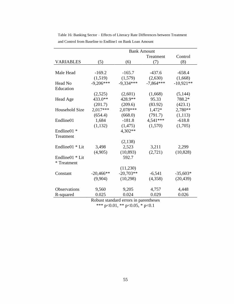
55
Table 16: Banking Sector – Effects of Literacy Rate Differences between Treatment
and Control from Baseline to Endline1 on Bank Loan Amount
Bank Amount
VARIABLES
(5)
(6)
Treatment
(7)
Control
(8)
Male Head -169.2 -165.7 -437.6 -658.4
(1,519) (1,579) (2,630) (1,668)
Head No
Education
-9,206*** -9,334*** -7,864*** -10,921**
(2,525) (2,601) (1,668) (5,144)
Head Age 433.0** 428.9** 95.33 788.2*
(201.7) (209.6) (83.92) (423.1)
Household Size 2,017*** 2,078*** 1,472* 2,780**
(654.4) (668.0) (791.7) (1,113)
Endline01 1,684 -181.8 4,541*** -618.8
(1,132) (1,475) (1,570) (1,705)
Endline01 *
Treatment
4,302**
(2,138)
Endline01 * Lit 3,498 2,523 3,211 2,299
(4,905) (10,893) (2,721) (10,828)
Endline01 * Lit
* Treatment
592.7
(11,230)
Constant -20,466** -20,703** -6,541 -35,603*
(9,904) (10,298) (4,358) (20,439)
Observations 9,560 9,205 4,757 4,448
R-squared 0.025 0.024 0.029 0.026
Robust standard errors in parentheses
*** p<0.01, ** p<0.05, * p<0.1

56
Table 17: Banking Sector – Robustness Table, Value Indicator Variable Triple
Interaction Coefficients
Baseline-Endline1 Baseline-Endline2
(1) (2) (3) (4)
VALUE
INDICATOR
Cutoff Bank Bank
Amount
Bank Bank
Amount
Already 1 Table 7 Table 8 -0.00461 12,412
Banked (Table 7) (Table 8) (0.0187) (7,981)
2 -0.0186 -8,253 -0.00616 -808.7
(0.0282) (8,088) (0.0215) (6,970)
Expenditures 50% Table 13 Table 14 -0.0302 2,098
(Table 13) (Table 14) (0.0217) (8,864)
75% -0.00203 8,758 -0.0355 8,148
(0.0275) (15,451) (0.0243) (13,623)
Debt 50% Table 11 Table 12 -0.000414 -10,648
(Table 11) (Table 12) (0.0227) (12,324)
75% -0.0142 -16,188 -0.0126 -13,566
(0.0239) (14,438) (0.0234) (15,045)
Businesses 50% Table 9 Table 10 -0.0111 -9,772
(Table 9) (Table 10) (0.0217) (8,492)
75% 0.0175 -20,101* -0.0258 -10,043
(0.0297) (12,015) (0.0225) (6,885)
Literacy 50% Table 15 Table 16 -0.0413* 5,141
(Table 15) (Table 16) (0.0220) (10,038)
75% -0.0571 -5,558 -0.0538** 8,592
(0.0393) (17,148) (0.0255) (15,276)
Robust standard errors in parentheses
*** p<0.01, ** p<0.05, * p<0.1

57
Table 18: Informal Sector – Treatment Differences from Baseline to Endline1 and
Endline2
(1) (2) (3) (4)
VARIABLES Informal Informal
Amount
Informal Informal
Amount
Male Head 0.00650 -1,882 0.00339 1,041
(0.0167) (2,859) (0.0162) (2,124)
Head No
Education
0.0661*** -3,107* 0.0620*** -76.50
(0.0113) (1,627) (0.0122) (1,813)
Head Age -0.00207*** 553.1*** -0.00166*** 379.9***
(0.000557) (89.46) (0.000631) (82.73)
Household
Size
0.0137*** 4,106*** 0.0103*** 2,687***
(0.00234) (538.7) (0.00269) (474.5)
Endline01 0.107*** 9,474***
(0.0259) (2,645)
Endline01 *
Treatment
-0.0509 1,028
(0.0324) (4,046)
Endline02 -0.0448** 46.04
(0.0214) (2,694)
Endline02 *
Treatment
-0.00881 979.6
(0.0294) (3,997)
Constant 0.631*** -12,399** 0.634*** -1,836
(0.0315) (5,070) (0.0305) (4,771)
Observations 9,205 9,205 8,549 8,549
R-squared 0.064 0.046 0.040 0.038
Robust standard errors in parentheses
*** p<0.01, ** p<0.05, * p<0.1

58
Table 19: Informal Sector – Value Indicator Variable Triple Interaction Coefficients for
Endline1
(1) (2)
VARIABLES Informal Informal
Amount
Already Banked 0.0391 7,487
(0.0700) (7,830)
Expenditures 0.00926 -2,096
(0.0647) (8,040)
Debt -0.0613 -4,491
(0.0591) (9,366)
Businesses 0.0335 -12,501
(0.0652) (7,931)
Literacy 0.00282 -8,650
(0.0646) (7,779)
Robust standard errors in parentheses
*** p<0.01, ** p<0.05, * p<0.1 All coefficients are for triple interaction terms. That is, the term that interacts high
value indicator, endline01, and treatment.
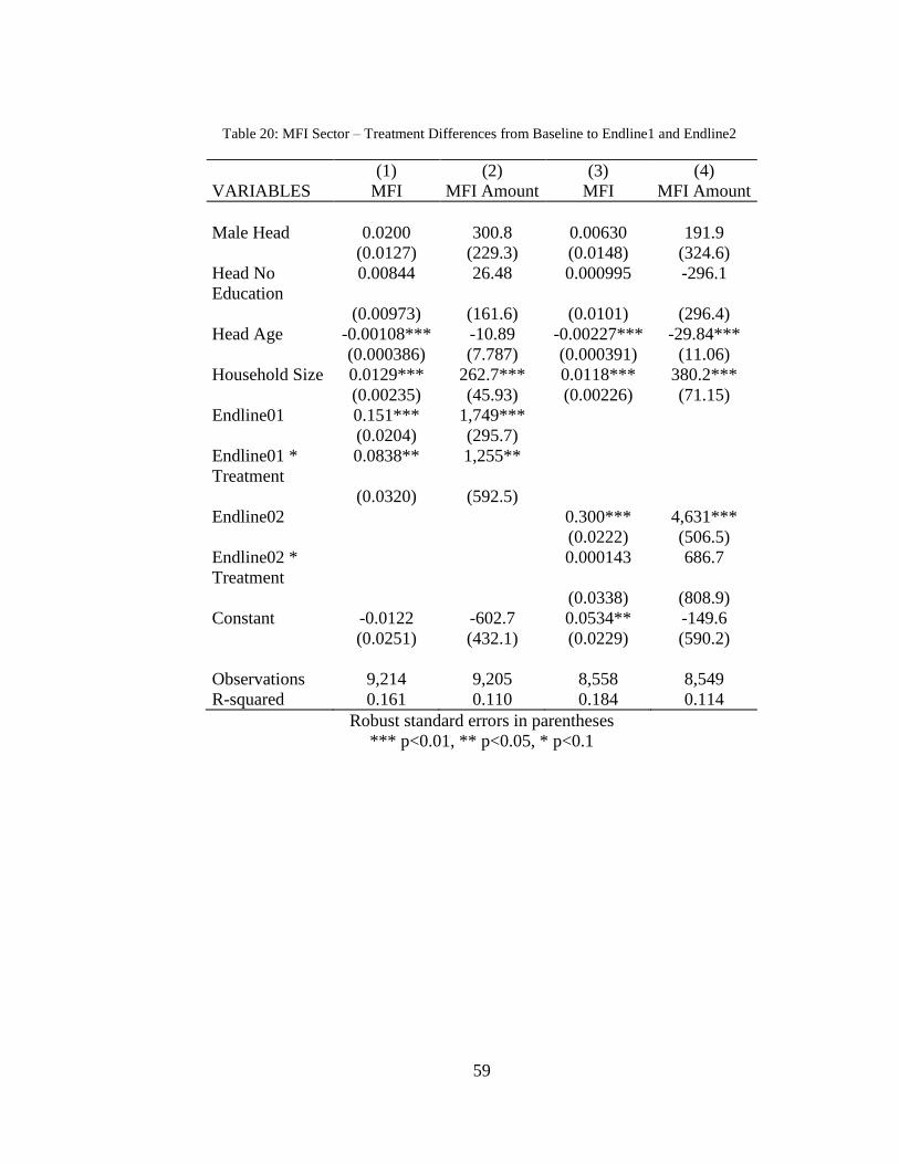
59
Table 20: MFI Sector – Treatment Differences from Baseline to Endline1 and Endline2
(1) (2) (3) (4)
VARIABLES MFI MFI Amount MFI MFI Amount
Male Head 0.0200 300.8 0.00630 191.9
(0.0127) (229.3) (0.0148) (324.6)
Head No
Education
0.00844 26.48 0.000995 -296.1
(0.00973) (161.6) (0.0101) (296.4)
Head Age -0.00108*** -10.89 -0.00227*** -29.84***
(0.000386) (7.787) (0.000391) (11.06)
Household Size 0.0129*** 262.7*** 0.0118*** 380.2***
(0.00235) (45.93) (0.00226) (71.15)
Endline01 0.151*** 1,749***
(0.0204) (295.7)
Endline01 *
Treatment
0.0838** 1,255**
(0.0320) (592.5)
Endline02 0.300*** 4,631***
(0.0222) (506.5)
Endline02 *
Treatment
0.000143 686.7
(0.0338) (808.9)
Constant -0.0122 -602.7 0.0534** -149.6
(0.0251) (432.1) (0.0229) (590.2)
Observations 9,214 9,205 8,558 8,549
R-squared 0.161 0.110 0.184 0.114
Robust standard errors in parentheses
*** p<0.01, ** p<0.05, * p<0.1

60
Table 21: MFI Sector – Value Indicator Variable Triple Interaction Coefficients for
Endline1
(1) (2)
VARIABLES MFI MFI Amount
Already Banked 0.0335 611.7
(0.0638) (1,133)
Expenditures -0.0508 -425.4
(0.0627) (1,146)
Debt 0.120* 2,318*
(0.0647) (1,386)
Businesses -0.0401 -992.0
(0.0637) (1,231)
Literacy 0.0211 914.3
(0.0669) (1,307)
Robust standard errors in parentheses
*** p<0.01, ** p<0.05, * p<0.1 All coefficients are for triple interaction terms. That is, the term that interacts high
value indicator, endline01, and treatment.

61
Table 22: Bank and MFI Loan Take-up Characteristics at Endline1 and 2
(1) (2)
VARIABLES Bank MFI
Household Size 0.00393*** 0.0127***
(0.00102) (0.00241)
Male Head 0.00333 0.00969
(0.00921) (0.0176)
Head Age 0.000798*** -0.00251***
(0.000243) (0.000499)
Head No Education -0.0190*** 0.000729
(0.00570) (0.0114)
Old Business 0.0160** 0.0807***
(0.00617) (0.0106)
Area Population (baseline) -1.53e-05 6.93e-05
(2.56e-05) (9.31e-05)
Already Banked (baseline) 0.0156** 0.0392
(0.00761) (0.0284)
Biz (baseline) -0.0110 -0.0110
(0.00873) (0.0307)
Expend (baseline) -0.00372 -0.0398
(0.00732) (0.0287)
Lit (baseline) 0.0197** -0.0336
(0.00972) (0.0258)
Own Land (baseline) 0.0171*** 0.00549
(0.00606) (0.0150)
Women Employment Index -0.0115* 0.0397***
(0.00619) (0.0136)
Income Index 0.0196*** 0.00719
(0.00540) (0.00740)
Labor Index -0.0157*** 0.0981***
(0.00542) (0.0134)
Consumption Index 0.0470*** 0.0141*
(0.00546) (0.00823)
Social Index 0.0271*** 0.0423**
(0.0102) (0.0197)
Constant 0.0106 0.260***
(0.0179) (0.0504)
Observations 12,689 12,689
R-squared 0.028 0.045
Robust standard errors in parentheses
*** p<0.01, ** p<0.05, * p<0.1 These regressions are built from the sample of everyone in the study, not solely people
who borrow, in order to look at loan take-up characteristics.
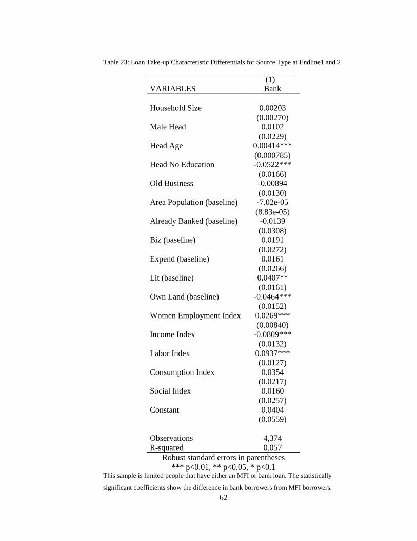
62
Table 23: Loan Take-up Characteristic Differentials for Source Type at Endline1 and 2
(1)
VARIABLES Bank
Household Size 0.00203
(0.00270)
Male Head 0.0102
(0.0229)
Head Age 0.00414***
(0.000785)
Head No Education -0.0522***
(0.0166)
Old Business -0.00894
(0.0130)
Area Population (baseline) -7.02e-05
(8.83e-05)
Already Banked (baseline) -0.0139
(0.0308)
Biz (baseline) 0.0191
(0.0272)
Expend (baseline) 0.0161
(0.0266)
Lit (baseline) 0.0407**
(0.0161)
Own Land (baseline) -0.0464***
(0.0152)
Women Employment Index 0.0269***
(0.00840)
Income Index -0.0809***
(0.0132)
Labor Index 0.0937***
(0.0127)
Consumption Index 0.0354
(0.0217)
Social Index 0.0160
(0.0257)
Constant 0.0404
(0.0559)
Observations 4,374
R-squared 0.057
Robust standard errors in parentheses
*** p<0.01, ** p<0.05, * p<0.1 This sample is limited people that have either an MFI or bank loan. The statistically
significant coefficients show the difference in bank borrowers from MFI borrowers.

63
Table 24: Loan Take-up Characteristic Means and Statistical Differences at Endline1
and 2
Variable Mean
(Standard Deviation)
Difference
(t-stat)
VARIABLES Bank MFI
Household Size 6.176412 6.249798 -0.0733856
(2.345757) (2.478231) (-0.8435)
Male Head 0.8937438 0.8575283 0.03621***
(0.3083184) (0.3495804) (2.9869)
Head Age 42.86879 41.09724 1.7715***
(10.10958) (9.555749) (5.149)
Head No Education 0.2085402 0.2976769 -0.08914***
(0.4064668) (0.4572984) (-5.6117)
Old Business 0.497992 0.5274966 -0.0295
(0.7010373) (0.7683152) (-1.0941)
Area Population (baseline) 300.6065 313.1471 -12.54059**
(145.2239) (144.6328) (-2.44)
Already Banked (baseline) 0.617443 0.5990299 0.0184131
(0.4862525) (0.490161) (1.0599)
Biz (baseline) 0.3548067 0.3629749 -0.0081682
(0.478692) (0.4809225) (-0.4789)
Expend (baseline) 0.4380575 0.3893829 0.0486746
(0.4963943) (0.4876761) (2.8004)
Lit (baseline) 0.5698712 0.5184586 0.051412***
(0.4953395) (0.4997265) (2.9031)
Own Land (baseline) 0.3568588 0.3034557 0.053403***
(0.4793109) (0.4598124) (3.2369)
Women Employment Index -0.01242 0.034934 -0.047354***
(0.4721381) (0.5093493) (-2.6588)
Income Index 0.1733441 0.0287202 0.144624***
(1.266404) (0.6780349) (4.8543)
Labor Index -0.0082099 0.0883006 -0.096510***
(0.412083) (0.4864337) (-5.7648)
Consumption Index 0.2544555 0.0136535 0.240802***
(0.8283451) (0.5493359) (10.9465)
Social Index 0.0331547 0.0162216 0.0169331
(0.3043466) (0.329294) (1.4714)
*** p<0.01, ** p<0.05, * p<0.1
64
Bibliography
Armendariz, Beatriz and Jonathan Morduch. 2010. The Economics of Microfinance.
Cambridge (MA): The MIT Press.
Banerjee, Abhijit, Dean Karlan, and Jonathan Zinnman. 2015. “Six Randomized
Evaluations of Microcredit: Introduction and Further Steps.” American
Economic Journal: Applied Economics 7(1): 1-21.
http://dx.doi.org/10.1257/app.20140287
Banerjee, Abhijit and Esther Duflo. 2007. “The Economic Lives of the Poor.” Author
manuscript National Center for Biotechnology Information. Originally published
Journal of Economic Perspectives 21(1): 141-167.
http://www.anderson.ucla.edu/faculty/bhagwan.chowdhry/Banerjee-Duflo.pdf
Banerjee, Abhijit and Esther Duflo. 2011. Poor Economics: A Radical Rethinking of the
Way to Fight Global Poverty. New York: PublicAffairs.
Banerjee, Abhijit, Esther Duflo, Rachel Glennerster, and Cynthia Kinnan. 2015. “The
Miracle of Microfinance? Evidence from a Randomized Evaluation.” American
Economic Journal: Applied Economics 7(1): 22-53.
http://dx.doi.org/10.1257/app.20130533
Chaia, Alberto, Aparna Dalal, Tony Goland, Maria Jose Gonzalez, Jonathan Morduch,
and Robert Schiff. 2009. “Half the World is Unbanked.” Financial Access
Initiative. http://mckinseyonsociety.com/downloads/reports/Economic-
Development/Half_the_world_is_unbanked.pdf
Collins, Daryl, Jonathan Morduch, Stuart Rutherford and Orlanda Ruthven. 2009.
Portfolios of the Poor: How the World’s Poor Live on $2 a Day. New Jersey:
Princeton University Press.
Cull, Robert, Asli Demirgüç-Kunt, and Jonathan Morduch. 2013. “Banks and
Microbanks.” Journal of Financial Services Research. 46(1): 1-53. doi:
10.1007/s10693-013-0177-z
Johnston Jr., Don, and Jonathan Morduch. 2008. “The Unbanked: Evidence from
Indonesia.” World Bank Economic Review. 22(3): 517-537.
https://doi.org/10.1093/wber/lhn016
Karlan, Dean and Jonathan Morduch. 2009. “Access to Finance.” Chapter 2, Handbook
of Development Economics, Volume 5.
http://www.financialaccess.org/publications-index/2009/access2finance
Katyal, Ritika. 2015 Aug 2. “India census exposes extent of poverty,” CNN.
http://www.cnn.com/2015/08/02/asia/india-poor-census-secc/
65
Maksudova, Nargiza, 2010. “Macroeconomics of Microfinance: How Do the Channels
Work?” Center for Economic Research and Graduate Education – Economics
Institute. Working Paper Series No. 423. https://www.cerge-
ei.cz/pdf/wp/Wp423.pdf
Microcredit Summit Campaign. 2015. “State of the Campaign.”
https://stateofthecampaign.org/2015/12/09/read-the-full-2015-report/
MicroLoan Foundation. 2007. “Charity or commerce? The different structures of
microfinance.” http://www.appg-
microfinance.org/files/Different%20forms%20of%20microfinance.pdf
Mookherjee, D. and A. Motta. 2016. “A theory of interactions between MFIs and
informal lenders.” Journal of Development Economics. 121(C): 191-2000.
Peachey, Stephen and Alan Roe. 2006. “Access to Finance – What Does It Mean and
How Do Savings Banks Foster Access.” World Savings Banks Institute.
https://www.microfinancegateway.org/sites/default/files/mfg-en-paper-access-
to-finance-what-does-it-mean-and-how-do-savings-banks-foster-access-jan-
2006_0.pdf
The World Bank. Poverty Headcount Ratio at $1.90 a day.
http://data.worldbank.org/indicator/SI.POV.DDAY?end=2013&locations=1W&
name_desc=false&start=1981&view=chart
Todaro, Michael and Stephen Smith. 2015. “Finance and Fiscal Policy for
Development.” In Economic Development, 12th Edition, 793. New Jersey:
Pearson.
Vanroose, Annabel and Bert D’Espallier. 2013. “Do Microfinance Institutions
Accomplish Their Mission? Evidence from the Relationship Between
Traditional Financial Sector Development and Microfinance Institutions’
Outreach and Performance.” Applied Economics 45(15): 1965-1982.
http://dx.doi.org/10.1080/00036846.2011.641932
World Bank Group. 2016. “Taking on Inequality.” Poverty and Shared Prosperity
Series. International Bank for Reconstruction and Development. Washington
DC. doi:10.1596/978-1-4648-0958-3.