Embed Size (px)
Citation preview

Competing Neural Networksas Models for
Non Stationary Financial Time Series- Changepoint Analysis -
Tadjuidje Kamgaing, Joseph
Vom Fachbereich Mathematik der Technische Universitat Kaiserslauternzur Erlangung des akademischen Grades
Doktor der Naturwissenschaften(Doctor rerum naturalium, Dr. rer. nat.)
genehmigte Dissertation
1. Gutachter: Prof. Dr. Jurgen Franke2. Gutachter: Prof. Dr. Michael H. Neumann
VOLLZUG DER PROMOTION: 14. FEBRUAR 2005
D 386

To my family.

AcknowledgmentI am profoundly grateful to my supervisor, Prof. Jurgen Franke. He provides mewith the topic, supports and encourages me along the way. On a personal level, I amdeeply thankful for the confidence he place in me. Further, I thank Prof. Michael H.Neumann who accepts to be the second advisor for my thesis.I would also like to thank Prof. Ralf Korn and through him the entire departmentof finance at the Fraunhofer ITWM (Institute for industrial mathematics) in Kaiser-slautern where I was provided an office, a friendly and creative atmosphere as wellas support to carry out my research.In particular, I thank all the people who sharedthe office with me during my thesis for the kindly, friendly and creative atmosphere.I am also grateful to Prof. Marie Huskova(Charles University, Prague) for the in-troductory discussion on test in changepoint analysis we had during her visit lastSeptember at the university of Kaiserslautern.I am deeply indebted to Dr. Jean Pierre Stockis and Dr. Gerald Kroisandt for theiruseful critics and the fruitful scientific discussion we use to have. Furthermore, Ialso deserve my gratitude to the entire Statistics research group of the university ofKaiserslautern for the friendly atmosphere and particularly, I deserve great respectto the secretary Mrs. Beate Siegler for this continuous achievement. Moreover,the funding of the Fraunhofer ITWM and Forschungsschwerpunkt Mathematik &Praxis of the mathematics department are highly appreciated.Last but not least, I am thankful to my family and friends for their permanent sup-port and to Elsy for her patience.May God bless and continue to inspire all the people I mentioned above and those Isilently and respectfully carry in my heart.

AbstractThe problem of structural changes (variations) play a central role in many scien-tific fields. One of the most current debates is about climatic changes. Further,politicians, environmentalists, scientists, etc. are involved in this debate and almosteveryone is concerned with the consequences of climatic changes.However, in this thesis we will not move into the latter direction, i.e. the study ofclimatic changes. Instead, we consider models for analyzing changes in the dynam-ics of observed time series assuming these changes are driven by a non-observablestochastic process. To this end, we consider a first order stationary Markov Chain ashidden process and define the Generalized Mixture of AR-ARCH model(GMAR-ARCH) which is an extension of the classical ARCH model to suit to model withdynamical changes.For this model we provide sufficient conditions that ensure its geometric ergodicproperty. Further, we define a conditional likelihood given the hidden process anda pseudo conditional likelihood in turn. For the pseudo conditional likelihood weassume that at each time instant the autoregressive and volatility functions can besuitably approximated by given Feedfoward Networks. Under this setting the con-sistency of the parameter estimates is derived and versions of the well-known Ex-pectation Maximization algorithm and Viterbi Algorithm are designed to solve theproblem numerically. Moreover, considering the volatility functions to be constants,we establish the consistency of the autoregressive functions estimates given someparametric classes of functions in general and some classes of single layer Feed-foward Networks in particular.Beside this hidden Markov Driven model, we define as alternative a Weighted LeastSquares for estimating the time of change and the autoregressive functions. For thelatter formulation, we consider a mixture of independent nonlinear autoregressiveprocesses and assume once more that the autoregressive functions can be approxi-mated by given single layer Feedfoward Networks. We derive the consistency andasymptotic normality of the parameter estimates. Further, we prove the convergenceof Backpropagation for this setting under some regularity assumptions.Last but not least, we consider a Mixture of Nonlinear autoregressive processes withonly one abrupt unknown changepoint and design a statistical test that can validatesuch changes.

CONTENTS v
ContentsAcknowledgment iii
Abstract iv
Some Abbreviations and Symbols viii
1 Introduction 11.1 Motivations . . . . . . . . . . . . . . . . . . . . . . . . . . . . . . 11.2 Outline . . . . . . . . . . . . . . . . . . . . . . . . . . . . . . . . 2
2 Generalized Nonlinear Mixture of AR-ARCH 42.1 Introduction . . . . . . . . . . . . . . . . . . . . . . . . . . . . . . 42.2 Model Description . . . . . . . . . . . . . . . . . . . . . . . . . . 5
2.2.1 Some Classical Cases . . . . . . . . . . . . . . . . . . . . . 52.3 Model Assumptions . . . . . . . . . . . . . . . . . . . . . . . . . . 62.4 Basic Properties Derived from the Model . . . . . . . . . . . . . . 7
2.4.1 Conditional Moments . . . . . . . . . . . . . . . . . . . . 82.4.2 Conditional Distribution . . . . . . . . . . . . . . . . . . . 9
2.5 Geometric Ergodicity . . . . . . . . . . . . . . . . . . . . . . . . . 102.5.1 Assumptions, Markov and Feller Properties of the Chain . . 112.5.2 Asymptotic Stability and Small Sets . . . . . . . . . . . . . 142.5.3 Geometric Ergodic Conditions for First Order GMAR-ARCH 152.5.4 Geometric Ergodic Conditions for Higher Order GMAR-
ARCH . . . . . . . . . . . . . . . . . . . . . . . . . . . . 162.6 Some Applications . . . . . . . . . . . . . . . . . . . . . . . . . . 21
2.6.1 Mixing Conditions . . . . . . . . . . . . . . . . . . . . . . 21
3 Neural Networks and Universal Approximation 233.1 Universal Approximation for some Parametric Classes of Functions 23
3.1.1 Generalities . . . . . . . . . . . . . . . . . . . . . . . . . . 233.1.2 Excursion to Lp Norm Covers and VC Dimension . . . . . 263.1.3 Consistency of Least Squares Estimates . . . . . . . . . . . 273.1.4 Universal Approximation . . . . . . . . . . . . . . . . . . . 28
3.2 Neural Networks as Universal Approximators . . . . . . . . . . . . 323.2.1 Density of Network Classes of Functions . . . . . . . . . . 323.2.2 Consistency of Neural Network Estimates . . . . . . . . . . 34
4 Hidden Markov Chain Driven Models for Changepoint Analysis in Fi-nancial Time Series 364.1 Discrete Markov Processes . . . . . . . . . . . . . . . . . . . . . . 364.2 Hidden Markov Driven Models . . . . . . . . . . . . . . . . . . . 38
4.2.1 Preliminary Notations . . . . . . . . . . . . . . . . . . . . 38

CONTENTS vi
4.3 Conditional Likelihood . . . . . . . . . . . . . . . . . . . . . . . . 394.3.1 Consistency of the Parameter Estimates . . . . . . . . . . . 40
4.4 EM Algorithm . . . . . . . . . . . . . . . . . . . . . . . . . . . . . 464.4.1 Generalities on EM Algorithms . . . . . . . . . . . . . . . 464.4.2 Forward-Backward Procedure . . . . . . . . . . . . . . . . 474.4.3 Maximization . . . . . . . . . . . . . . . . . . . . . . . . . 504.4.4 An Adaptation of the Expectation Maximization Algorithm 52
4.5 Viterbi Algorithm . . . . . . . . . . . . . . . . . . . . . . . . . . . 52
5 Nonlinear Univariate Weighted Least Squares for Changepoint Analy-sis in Time Series Models 545.1 Nonlinear Least Squares . . . . . . . . . . . . . . . . . . . . . . . 54
5.1.1 Preliminaries . . . . . . . . . . . . . . . . . . . . . . . . . 565.1.2 Consistency under Weak Assumptions . . . . . . . . . . . . 575.1.3 Asymptotic Normality . . . . . . . . . . . . . . . . . . . . 60
5.2 Nonlinear Weighted Least Squares . . . . . . . . . . . . . . . . . . 635.2.1 Preliminaries . . . . . . . . . . . . . . . . . . . . . . . . . 655.2.2 Consistency . . . . . . . . . . . . . . . . . . . . . . . . . . 685.2.3 Asymptotic Normality . . . . . . . . . . . . . . . . . . . . 74
6 Multivariate Weighted Least Squares for Changepoint Analysis in TimeSeries Models 766.1 Multivariate Least Squares . . . . . . . . . . . . . . . . . . . . . . 76
6.1.1 Consistency and Asymptotic Normality . . . . . . . . . . . 786.2 Nonlinear Multivariate Weighted Least Squares . . . . . . . . . . . 79
6.2.1 Preliminaries . . . . . . . . . . . . . . . . . . . . . . . . . 806.2.2 Consistency and Asymptotic Normality . . . . . . . . . . . 82
7 A Numerical Procedure: Backpropagation 847.1 Convergence of Backpropagation . . . . . . . . . . . . . . . . . . . 84
7.1.1 Asymptotic Normality . . . . . . . . . . . . . . . . . . . . 88
8 Excursion to Tests in Changepoints Detection 918.1 Generalities . . . . . . . . . . . . . . . . . . . . . . . . . . . . . . 918.2 Test for Changes in Nonlinear Autoregressive Model . . . . . . . . 91
9 Case Studies 969.1 Computer Generated Data . . . . . . . . . . . . . . . . . . . . . . 96
9.1.1 Mixture of Stationary AR(1) and Weighted Least SquaresTechniques . . . . . . . . . . . . . . . . . . . . . . . . . . 96
9.1.2 GMAR-ARCH(1) and Hidden Markov Techniques . . . . . 989.2 Forecast of Daily Stock Values and Market Strategy . . . . . . . . 100
9.2.1 Model for Daily Stock Values . . . . . . . . . . . . . . . . 100

CONTENTS vii
9.2.2 Forecast of Transformed Daily Values of a DAX Compo-nent: BASF . . . . . . . . . . . . . . . . . . . . . . . . . . 103
9.2.3 Market Strategy . . . . . . . . . . . . . . . . . . . . . . . . 1069.3 GMAR-ARCH as Model for DAX Return . . . . . . . . . . . . . . 108
10 Conclusion and Outlook 11010.1 Conclusion . . . . . . . . . . . . . . . . . . . . . . . . . . . . . . 11010.2 Outlook . . . . . . . . . . . . . . . . . . . . . . . . . . . . . . . . 111
A An Introduction to Neural Networks 112A.1 Preliminaries and Network Description . . . . . . . . . . . . . . . . 112
A.1.1 Some Examples of Activation Functions . . . . . . . . . . . 113A.2 Neural Networks in Practice . . . . . . . . . . . . . . . . . . . . . 115
A.2.1 Least Squares . . . . . . . . . . . . . . . . . . . . . . . . . 115A.2.2 Backpropagation . . . . . . . . . . . . . . . . . . . . . . . 115
A.3 Some Technical Remarks . . . . . . . . . . . . . . . . . . . . . . . 116A.3.1 Input . . . . . . . . . . . . . . . . . . . . . . . . . . . . . 116A.3.2 Local minima . . . . . . . . . . . . . . . . . . . . . . . . . 116A.3.3 Number of Hidden Neurons . . . . . . . . . . . . . . . . . 116
References 117
Some Abbreviations and Symbols
Abbreviationslim limitmax maximummin minimumsup supremumi.i.d. independent identically distributedM.C. Markov Chain
Symbolsexp(x) = ex
|x| Absolute value of x‖θ‖ Norm of the vector θZ = · · · ,−2,−1, 0, 1, 2, · · · N = 0, 1, 2, · · · R Set of real numbersRd d-dimensional Euclidian spaceP( A ) Probability of the set AP( A | B ) Conditional probability of the set A given the set BE( X ) Expectation of the random variable XE( X | A ) Conditional expectation of the random variable X
given the information contained in AN (0, 1) Standard Normal distributionN (0,Σ) Multivariate Normal distribution with mean vector 0
and covariance matric Σ

1
1 Introduction
1.1 MotivationsIn various fields one has to analyze data collected over long periods of observation.Time series models account for one of the most widely used tools in data analysis.The classical time series behavior is to assume stationary stochastic processes asmodel for these data under the main hypothesis that these data satisfy some stabil-ity conditions or invariance properties. This hypothesis is satisfied by many linearmodels that have now been intensively used for many decades. For example the firstorder autoregressive processes
Yt = αYt−1 + εt,
for which |α| < 1 and w.l.o.g the residuals εt are random variables with mean zeroand unit variance, e.g. N (0, 1) . The following plot contains examples of suchcomputer-generated processes for which we have considered α = 0.97 and −0.97respectively.
0 200 400 600 800 1000 1200−10
−5
0
5
10
15
0 200 400 600 800 1000 1200−15
−10
−5
0
5
10
15
Figure 1.1: Stationary First Order Autoregressive Processes
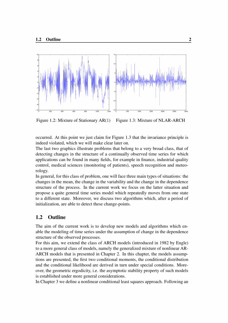
However, these assumptions (e.g. of invariance in time) are frequently satisfiedonly over periods of limited length, in other words they are usually only locally sat-isfied as one can observe in some very specific cases. We can consider for examplea simple mixture of two stationary first order autoregressive processes as illustratedby Figure 1.2. Under this setting the regular variation of the structure is clearlyexhibited and human eyes can also be used to make the decision on such changes.Unfortunately, it is not always the case that this violation of the invariance propertyis clearly observable just by using human eyes as confirmed by Figure 1.3. In fact,in this picture it is less obvious than in the previous one where the changes may have
1.2 Outline 2
0 200 400 600 800 1000 1200−10
−8
−6
−4
−2
0
2
4
6
8
10
Figure 1.2: Mixture of Stationary AR(1)
0 500 1000 1500 2000 2500 3000−15
−10
−5
0
5
10
15
Figure 1.3: Mixture of NLAR-ARCH
occurred. At this point we just claim for Figure 1.3 that the invariance principle isindeed violated, which we will make clear later on.The last two graphics illustrate problems that belong to a very broad class, that ofdetecting changes in the structure of a continually observed time series for whichapplications can be found in many fields, for example in finance, industrial qualitycontrol, medical sciences (monitoring of patients), speech recognition and meteo-rology.In general, for this class of problem, one will face three main types of situations: thechanges in the mean, the change in the variability and the change in the dependencestructure of the process. In the current work we focus on the latter situation andpropose a quite general time series model which repeatedly moves from one stateto a different state. Moreover, we discuss two algorithms which, after a period ofinitialization, are able to detect these change-points.
1.2 OutlineThe aim of the current work is to develop new models and algorithms which en-able the modeling of time series under the assumption of change in the dependencestructure of the observed processes.For this aim, we extend the class of ARCH models (introduced in 1982 by Engle)to a more general class of models, namely the generalized mixture of nonlinear AR-ARCH models that is presented in Chapter 2. In this chapter, the models assump-tions are presented, the first two conditional moments, the conditional distributionand the conditional likelihood are derived in turn under special conditions. More-over, the geometric ergodicity, i.e. the asymptotic stability property of such modelsis established under more general considerations.In Chapter 3 we define a nonlinear conditional least squares approach. Following an

1.2 Outline 3
idea of Franke et al we prove the asymptotic consistency of the autoregressive func-tion estimates given some parametric classes of functions. This result is particularlyvalid for some classes of feedfoward network functions.As alternative to the conditional nonlinear least squares defined in Chapter 3, inChapter 4 (based on the hidden process) we define a conditional likelihood fromwhich we derive a pseudo conditional log-likelihood. Indeed, for the pseudo condi-tional log-likelihood we assume that the autoregressive and volatility functions canbe suitably approximated by feedfoward networks with a fixed number of hiddenneurons. Under this setting the consistency of the parameter estimates is provenfor the pseudo conditional log-likelihood. Moreover, a version of the Expectation-Maximization (EM) Algorithm introduced by Baum et al is proposed to solve theproblem numerically.In Chapter 5, focusing on the changes driven by the autoregressive functions, wepropose some weighted least squares techniques for estimating the changes in thedynamics of the observed process. Under the assumption that the autoregressivefunction can be suitably approximated by feedfoward network and under some reg-ularity assumptions, the consistency and asymptotic normality of the parameter es-timated are proven. The results of this chapter are extended in Chapter 6, wherewe assume a multivariate time series. Furthermore, in Chapter 7, following an ideaby White [88], we prove the convergence and asymptotic normality of Backpropa-gation (a stochastic approximation algorithm that can be used to solve the problemnumerically considering the weighted least squares).Chapter 8 gives a short introduction to the problem of test in changepoint analysis.In fact, a nonlinear autoregressive case with only one abrupt unknown change isconsidered and a test for validating the change is designed under some regularityassumptions.In chapter 9 some numerical applications of the the pseudo conditional log-likelihoodor hidden Markov techniques (developed in Chapter 4) and weighted least squarestechniques (developed in Chapter 5) are presented. Indeed we present the results forthe computer-generated data and real-life financial data as well.The current work is summarized in Chapter 10 where some open questions of par-ticular interest are exhibited. Finally, a brief introduction to Neural Networks ispresented in Appendix A.

4
2 Generalized Nonlinear Mixture of AR-ARCH
2.1 IntroductionSince many decades time series models have been intensively used for analyzing thedynamic behavior of medical, social, economic, financial variables, etc. The mostpopular choices are linear models as autoregressive (AR), Moving Average (MA)and Mixed Autoregressive Moving Average (ARMA) processes. The linear time se-ries models became very popular essentially because of their theoretical tractabilityand partly because they have been incorporated into many standard statistical soft-ware packages. Despite their popularity, linear models suffer from several draw-backs. These include their inability to capture dynamic patterns such as asymmetryand volatility clustering, just to name a few.In the last decades, many nonlinear time series models with successful applicationshave been proposed. We can mention, for example, the Autoregressive conditionalheterokedastic models introduced in 1982 [23] by Engle (the Nobel Laureate) tomodel financial volatility. Additionally, we can refer to the book by Tong [84] fora general introduction on the nonlinear time series models. However, the nonlineartime series models also have their limitations. The main drawback is that most of thenonlinear models are designed just to describe specific nonlinear pattern, i.e. theymay suffer from a lack of flexibility. Therefore a nonlinear model will be success-ful only if it is applied to a very specific class of data. An exception in this classis the so-called non parametric Artificial Neural network, that with its ”Universalapproximation property” is able to capture any nonlinear pattern into the data. Nev-ertheless, Neural Network can suffer from identifiability problem and therefore mayalso be vulnerable. In spite of the universal approximation property neural networkmay locally be inefficient if we consider very complex dynamical structures that forexample exhibit local instability.Since the end of the 1980s the Hidden Markov model (or Switching Markov model)in the framework of Hamilton [41] (who did some pioneer applications of thismodel to the US gross domestic product-GDP- growth) is gaining popularity. Thesemodels consist of different sub-models that can account for the behavior of the ob-served data in different dynamics. By allowing switches between these differentsub-models, the new model (called mixture model) is able to represent more com-plex dynamical systems. Therefore, this models provides more flexibility than clas-sical linear and nonlinear models. In literature one can find quite a lot of publicationson this topic see, e.g. Hamilton ( [41], [42], [43]), Elliot et al [22], Macdonald etal [64], Wong and Li [94], Stockis et al [83]. In general, the related publicationscontain a lot about the practical applications of the models but very few on their sta-tistical properties. In this section we will consider a class of Generalized NonlinearMixture of AR-ARCH for which we will give a mathematical description, derivesome of their basic properties and finally present and prove some results on theirgeometric ergodicity.

2.2 Model Description 5
2.2 Model DescriptionIn this section we present a general description of our model and give some assump-tions that will be used in this chapter. Let us first present some definitions.
Definition 2.2.1 Let us consider the hidden stochastic process Qt, t ∈ N thattakes its value on IK = 1, · · · , K, where K is a given positive integer. Let us nowdefine for k ∈ IK the stochastic processes
St,k(ω) =
1 if k = Qt(ω)
0 otherwise,(2.1)
and in turn define the process St(ω) = (St,1(ω), · · · , St,K(ω)) on K ⊂ RK the setof all its possible realizations.
More details on the stochastic nature of Qt will be given as one will need them, forexample we will start by assuming the hidden stochastic process to be a stationaryMarkov Chain.Consider a time series Xt, t = 0, 1, 2, · · · . For this series, we will assume thatthe underlying process has some changes in its dynamics. These changes can bemodeled via a Hidden Markov Chain. This type of situation can be modeled withthe help of a Generalized Mixture of AR-ARCH (GMAR-ARCH ), i.e. a modeldefined as it follows.
Definition 2.2.2 Generalized Mixture of AR-ARCH (GMAR-ARCH)A stochastic process is called a GMAR-ARCH of order K and p if
Xt =K∑
k=1
St,k(mk(Xt−1) + σk(Xt−1)εt,k) with St,k =
1 for k = Qt
0 otherwise,(2.2)
where the processes εt,k are i.i.d. random variables, independent of Xt−1 =(Xt−1, · · · , Xt−p); and mutually independent for each k 6= j = 1, · · · , K, andw.l.o.g. Eεt,k = 0, Eε2t,k = 1. The mk(u) and σk(u) are unknown real valuedfunctions.
2.2.1 Some Classical Cases
From the model defined in 2.2.2 one can derive some classical and well-knownspecial cases. In this light let us consider several situations.If we were to consider the special case where K = p = 1 and were given
m(x) = ax and σ(x) = c > 0,
2.3 Model Assumptions 6
the process simply describes an AR (1). Similarly, one can represent a classicalARCH (1 ) model by choosing
m(x) ≡ 0 and σ(x) =√ω + αx2, ω > 0, α ≥ 0.
However, ifm(x) = ax and σ2(x) = σx2,
the process is reduced to the discrete time version of a geometric Brownian Motionas considered by Black and (the Nobel laureate) Scholes for their well-known optionpricing model.Still, we have to observe that our model differs from this classical model, let usconsider for example K = 2. If we then assume St,1 = 1 for t = 1, · · · , τ0 andSt,2 = 1 for t = τ0 + 1, · · · , n, the model defined in equation 2.2 experiences asingle structural change as the parameters of the model abruptly change after τ0.In the case where K ≥ 2, we can, e.g. consider that St as an i.i.d. sequenceof random variables. Each dynamic variable is independent of the past and futuredynamics and the processXt may switch back and forth between different dynamics.That is the case under consideration in Quandt ( [78], 1972 ) and the mixture ofautoregressive, i.e. the model of equation 2.2 for which we assume that the St arei.i.d. sequences of random variables, all volatility functions are constant and the mk
are linear, i.e.
mk(u) =
p∑
i=1
αk,iui
as proposed by Wong and Li [94]. This is just a special case of such models.These models are able to capture time series with several dynamics, but they sufferfrom different drawbacks. The model with one abrupt change is too restrictive inpractice since it admits only one change. As time series are correlated by nature, itseems more convenient to expect that each dynamic depends on the past happenings.To overcome the limitations we can find in some classical models we can makevarious assumptions on the hidden process, e.g. we can assume it to be be a firstorder stationary Markov Chain. Let us now present some general assumptions forthe model.
2.3 Model AssumptionsLet us consider the εt,k to be independent of Gt−1 = σXr, r ≤ t − 1, addi-tionally, conditioned on the past information we also assume that St and the εt,k areuncorrelated. Moreover we assume
P(Qt = j | Qt−1 = i, Qt−1, Qt−2 · · · ,Gt−1) = P(Qt = j | Qt−1 = i). (2.3)
Themk : Rp −→ R and σk : Rp −→ (0,∞)
2.4 Basic Properties Derived from the Model 7
are unknown functions which in general have to be estimated;K is the given numberof states or dynamics in the process, p is the order of the underlying NLAR −ARCH(p) processes
Xt = mk(Xt−1) + σk(Xt−1)εt,k,
with Xt−1 = (Xt−1, · · · , Xt−p) . However, p does not need to be the same for allthe underlying NLAR −ARCH. Nevertheless, we can always assume it by takingp = maxkp1, · · · , pk if we were to be given different orders for the underlyingNLAR − ARCH dynamics. Moreover we do not need the autoregressive and thevolatility functions to depend on the same parameter, i.e. we can choose autore-gressive functions of order p and volatility functions of order q as in Masry andTjostheim [67].As announced earlier, various assumption can be made on Qt, t = 0, 1, · · · , defined on 1, · · · , K, e.g. one can assume it to be an irreducible and aperi-odic Markov Chain (M.C.), i.e. a stationary M.C. with initial stationary distribu-tion π = (π1, · · · , πk) and transition probability matrix (ai,j) . A short introductionon discrete Markov processes will be presented in Chapter 4 and for more generaltheory and approaches on Markov models we will refer to the books by Tong [84],Meyn et al [70] and Duflo [20] among others.
2.4 Basic Properties Derived from the ModelIt is clearly observable that
St = (St,1, · · · , St,K),
with its entries St,k, k = 1, · · · , K defined as in equation 2.2 , inherits the propertiesof Qt. For example if we assume Qt is M.C. with value on IK , St will consequentlybe a M.C. on K for which one should have the following basic properties.
P(St,j = 1 | St−1,i = 1) = P(Qt = j | Qt−1 = i)
= ai,j, (2.4)
where the ai,j are the entries of transition probability matrix. We also have
ESt,k = P(Qt = k)
= πk, (2.5)
with
π1 + · · ·+ πK = 1 (2.6)
since π is the initial stationary distribution of Qt.In the next two subsections we strengthen the Markov assumption on Qt and sim-ply assume the St to be a sequence of i.i.d. random variables. Under this simpleassumption we give an impression of how one can compute the conditional expecta-tion, conditional variance and conditional distribution for our model given the pastinformation.

2.4 Basic Properties Derived from the Model 8
2.4.1 Conditional Moments
The purpose of this section is to compute first and second order conditional expec-tation of Xt given the past observations Xt−1. Assuming St is a sequence of i.i.d.random variable it follows trivially that
E(St,k | Xt−1 = x) = πk.
Given this property, we can derive the conditional expectation and the conditionalvariance of Xt with respect to the past information Xt−1, what we summarize in thefollowing lemma.
Lemma 2.1 Under the model assumptions and assuming St i.i.d. sequences of ran-dom variables it follows that the conditional expectation of Xt with respect to thepast realizations Xt−1 is defined as
E(Xt | Xt−1 = x) =K∑
k=1
πkmk(x) (2.7)
and its conditional variance is defined as
var(Xt | Xt−1 = x) =K∑
k=1
πk(m2k(x) + σ2
k(x))
−(
K∑
k=1
πkmk(x)
)2
. (2.8)
Remark 2.2 For the conditional variance, let us observe that
K∑
k=1
πkm2k(x)−
(K∑
k=1
πkmk(x)
)2
is non negative since the square function is convex. It takes the value zero if weconsider mj(x) = mk(x) for all j, k = 1, · · · , K. Therefore, we can derive thesmallest value of the volatility, which we can write as follows
K∑
k=1
πkσ2k(x).
We can consider the latter as baseline for the volatility at each time instant.
Let us now present a proof of the above lemma.Proof: By definition, the conditional expectation can be written as
2.4 Basic Properties Derived from the Model 9
E(Xt | Xt−1 = x) =K∑
k=1
mk(x)E(St,k | Xt−1 = x)
+
K∑
k=1
σk(x)E(St,kεt | Xt−1 = x).
For the first part of this equation we need to apply the result from equation 2.5 andfor the second part we use the fact that St and εt are uncorrelated, conditioned onthe past information.For the proof of the conditional variance, it suffices to derive the conditional secondmoment, i.e.
E(X2t | Xt−1 = x) =
K∑
k=1
πk(m2k(x) + σ2
k(x)).
To prove it let us remark that
X2t =
K∑
k=1
St,k(m2k(Xt−1) + 2εtmk(Xt−1)σk(Xt−1) + ε2tσ
2k(Xt−1))
and the proof is similar to that for the conditional expectation. The conditionalvariance is then obviously derived.
Once we have derived the conditional moments, let us now derive the conditionaldistribution under mild assumptions.
2.4.2 Conditional Distribution
Since in the case of the mixture of time series the conditional distribution can bemulti-modal, one has the feeling that the conditional mean may not be the bestpredictor of the future values of the series. However, the merits of our model partlyfind their justification in their ability to provide nice formula for the conditionaldistribution with respect to the past information. For sake of simplicity, if we thenassume that the εt,i = εt,j = εt ∀ i, j = 1, · · · , K, are i.i.d. normally distributed, theconditional distribution of Xt given Xt−1 = x is given in the following lemma.
Lemma 2.3 We consider the model assumptions, St i.i.d. random variables and the
εt,i = εt,j = εt ∀ i, j = 1, · · · , K,
i.i.d. standard normally distributed. Then, it follows that
F (Xt | Xt−1 = x) =
K∑
k=1
πkΦ
(Xt −mk(x)
σk(x)
), (2.9)
where Φ is the cumulative distribution of the standard normal distribution.
2.5 Geometric Ergodicity 10
Proof: To prove it, let us first consider its conditional density, i.e.,
f(Xt | Xt−1 = x) =K∑
k=1
f(Xt, Qt = k | Xt−1 = x)
= f(Xt | Qt = k,Xt−1 = x)f(Qt = k | Xt−1 = x)
where f(Qt = k | Xt−1 = x) denotes the conditional probability weights of Qt
given Xt−1 = x.By an application of the Tower property and the definition of the conditional density,we obtain
f(Qt = k | Xt−1 = x) = f(St,k = 1 | Xt−1 = x)
= E(E(St,k | Xt−1 = x,Qt−1) | Xt−1 = x)
= πk
by equation 2.5. The integration of the conditional density with respect to Xt con-cludes the proof of the conditional distribution.
Having this representation one can define the conditional log-likelihood as
l =∑
t
log
K∑
k=1
πkΦ
(Xt −mk(x)
σk(x)
). (2.10)
However, we have to remark that, even under i.i.d. assumption on the St, a di-rect computation of this quantity (l) may be computationally too demanding. Thisis partly because we have to compute the logarithm of a sum. To overcome thistype of problem, we will propose an alternative solution for the computation of theconditional log-likelihood in a later chapter by making use of the hidden structure.
2.5 Geometric ErgodicityIn time series analysis, we are generally interested in the stability of the model,i.e., in ergodicity. This is partly because of the theoretical importance of stationar-ity. However, it seems to appear that geometric ergodic models are very importantsince the rate of approaching stationarity ought to be fast enough for the stationaryassumption to be relevant. Stability will therefore be the main purpose of this sec-tion in which we will find some sufficient conditions for determining whether theswitching nonlinear autoregressive processes are geometric ergodic, what we willmake clear in the coming sections.Several authors have devoted works on stability conditions for nonlinear autoregres-sive processes, this is the case in Doukhan and Ghindes [19], Tong [84], Gueganand Diebolt ( [38], 1994), Maercker ( [66], 1995), Masry and Tjostheim [67] ormore recently Z. Lu [63]just to name a few. In the switching setting we have some
2.5 Geometric Ergodicity 11
work by Stockis et al ( [83], on mixture of first order nonlinear AR-ARCH) andYao et al [98] under some particular assumptions, among others.Under weaker assumptions, we propose the geometric ergodic property of our pro-cess as defined in equation 2.2. For this purpose, we need to rely on (St, Xt)
′ andtherefore it will suffice to prove that ζt = (St, Xt, · · · , Xt−p+1)
′ is a geometric er-godic Markov Chain.
2.5.1 Assumptions, Markov and Feller Properties of the Chain
Before we move toward the geometric ergodic proof, let us first set down someassumptions and derive some properties that will help us to achieve our goal.
A. 2.4 (Regularity Assumptions)
1. The process Qt is a first order stationary Markov Chain (S.M.C.) which isirreducible and aperiodic with initial stationary distributionπ = (π1, · · · , πK)and transition probability matrix A.
2. The i.i.d. random variables εt have positive probability density function φ onR that is continuous, moreover they have zero expectation and finite variance;w.l.o.g. we will assume the latter equal to 1.
3. The functions mk and σk are continuous on Rp , and σk are bounded awayfrom zero, i.e. infσk(u) : u ∈ Rp > 0 ∀ k ∈ 1, · · · , K.
4. There exist αk, dk ∈ Rp with dk,i ≥ 0, i = 1, · · · , p, such that, as ‖u‖ → ∞,
mk(u) =
p∑
i=1
αk,iui + o(‖u‖) and σ2k(u) =
p∑
i=1
dk,iu2i + o(‖u‖2).
As alternative to A.2.4-1, we can simply consider an irreducible and aperiodic chainand the stationary condition will follow directly, hence, we will avoid any redun-dancy.Assumptions A.2.4-2 to 4 are analogous conditions due to Masry and Tjostheim[67] where they considered stability conditions for NAR-ARCH (p). The differencein our context is due to the GMAR-ARCH (p) with continuous autoregressive andvolatility functions. Moreover, assumption A.2.4 4 does not imply that the modelhas to be parametric or linear in a certain sense. It just means that if the previousrealizations of the observed process are large enough, one can prevent any explosionof the process to infinity by approximating the process with a parametric model asdefined in the assumption.Having stated the above assumptions (A.2.4), let us first state and prove that ζt is aMarkov Chain.

2.5 Geometric Ergodicity 12
Lemma 2.5 Assuming the model assumptions and Qt first order stationary M.C., itfollows that ζt is a Markov Chain.
Proof: To prove the above assertion, let us rewrite ζt =(StUt
)with Ut =
(Xt, · · · , Xt−p+1)′ and prove the claim.Since St is a M.C., by Definition 6.1.3 in Duflo [20], there exists a measurable func-tion F and a sequence ηt of identically distributed random variables, independent ofεt, St−1 such that
St = F (St−1, ηt).
Writing
Ut =
Xt
.
.
.Xt+1−p
=
∑Kk=1 St,k(mk(Xt−1) + σk(Xt−1)εt)
Xt−1
.
.Xt+1−p
it follows that ζt is a Markov Chain with state space Ω ⊂ K × Rp.
Given the previous lemma, we can now make sure that ζt satisfies some well-knownand useful Markov properties.
Lemma 2.6 Under the model assumptions and A. 2.4 the chain ζt is irreducibleand aperiodic. Moreover the chain has the Feller property, i.e. consider P as thetransition probability kernel, then the mapping
Ph(ζ) =
∫P (ζ, dy)h(y), ζ ∈ K × Rp
is bounded and continuous whenever h is a bounded, continuous function.
Proof: Consider A ∈ B, A ⊆ Ω = K × Rp with λ(A) > 0, (λ = νµp is theproduct of the counting measure ν on IK = 1, · · · , K and the Lebesgue measureµp on Rp) and ζ1 =
(SU1
). Using the technique by Tong [84] for the generalized
nonlinear autoregressive model of order p that we extend to our model.First, we remark that is it is sufficient to consider A = s∗ × B for s∗ ∈ K andB ⊆ Rp a Borel set, as, due to the finiteness of K, any A can be written as finitedisjoint union of such sets. Furthermore, choose k∗ such that S∗j = 1 for j = k∗, 0else. We start with the case case p = 1, i.e. Xt = Ut. Then, the one-step transitionprobability give that we start in ζ1 = (S1, X1)′ = (s, x)′ is with Sj = 1 for j = l, 0

2.5 Geometric Ergodicity 13
else:
P((
S2
X2
)∈ A | S1 = s,X1 = x
)
= P (Q2 = k,X2 ∈ B | Q1 = l, X1 = x)
= P (X2 ∈ B | Q2 = k,Q1 = l, X1 = x)P(Q2 = k|Q1 = l, X1 = x)
= al,kP(mk(x) + σk(x)ε2 ∈ B)
= al,k
∫
B
1
σk(x)φ
(u−mk(x)
σk(u)
)du
= al,kbk(x) (2.11)
For more than one step, we have analogous
P((
S3
X3
)∈ A | S1 = s,X1 = x
)
=K∑
j=1
al,jaj,k
∫
B
∫
R
1
σk(y)φ
(u−mk(y)
σk(y)
)1
σj(x)φ
(u−mj(x)
σj(u)
)dydu
=
K∑
j=1
al,jaj,kbj,k(x) (2.12)
and doing so iteratively one obtains
P((
St+1
Xt+1
)∈ A | S1 = s,X1 = x
)=
K∑
j1,··· ,jt=1
al,j1 · · ·ajt,kbj1,··· ,jt,k(x)
As φ is strictly positive and the σk(x) are bounded away from 0 by A. 2.4, there issome δx,t > 0 such that bj1,··· ,jt,k(x) ≥ δx,t > 0 for all j1, · · · , jt, k, i.e.
P((
St+1
Xt+1
)∈ A | S1 = s,X1 = x
)≥ δx,t(A
t)l,k > 0 (2.13)
for some t as the Markov chain Qt is irreducible by A. 2.4. Therefore, A can bereached from any initial state
(sx
), and ζt is therefore irreducible and, analogously
due to the aperiodicity of Qt aperiodic.For the case p > 1, the argument is essentially the same. One only has to take careof the fact that Ut,j = Ut−1,j−1, 2 ≤ j ≤ p such that usually an arbitrary set A withpositive measure can be reached only after at least p steps.Hence the chain ζt is irreducible and aperiodic. That ζt has a Feller propertyfollows from the definition of the weak Feller property, the fact that the mk, σk arecontinuous and the σk are bounded away from zero.
In the coming sections we recall what it means for a stochastic process to satisfy thegeometric ergodic property, present characterization and derive the property for themixture of first order and higher GMAR-ARCH as well. Last but not the least, atthe end of this chapter we derive some consequences of the asymptotic stability.

2.5 Geometric Ergodicity 14
2.5.2 Asymptotic Stability and Small Sets
Let us first present two preliminary definitions. For this purpose, let us consider Xn
Markov Chain on (X,B(X)) with transition kernel P.
Definition 2.5.1 Small set and petite set
1. A setC ∈ B(X) is called a small set if there exists anm > 0, and a non-trivialmeasure νm on B(X), such that for all x ∈ C,B ∈ B(X),
Pm(x,B) ≥ νm(B)
2. A set C ∈ B(X) is νa-petite if there exists a probability measure a = a(n)on N such that
∞∑
n=0
a(n)P n(x,B) ≥ νa(B), ∀x ∈ C,B ∈ B(X),
where νa is a non trivial measure on B(X).
From the above definitions, one can observe that a small set is obviously a petite set.
Lemma 2.7 Let us assume ζt satisfies the conditions of Lemma 2.6. Supposethere exist a small set C, a non negative measurable function g, and constants 0 <r < 1, γ > 0 and B > 0 such that
E(g(ζt) | ζt−1 =
(S
x
))< rg
(S
x
)− γ,
(S
x
)6∈ C
E(g(ζt) | ζt−1 =
(S
x
))< B,
(S
x
)∈ C.
Then the chain ζt is geometrically ergodic, i.e. ζt is ergodic with stationary prob-ability distribution measure λ and there exists a positive constant ρ < 1 such that
‖P n(. | ζ)− λ‖TV = O(ρn),
where
P n(B | ζ) = P (ζn ∈ B | ζo = ζ), B ∈ B
is the conditional distribution of ζn given ζo = ζ and ‖ ‖TV is the total variationnorm.

2.5 Geometric Ergodicity 15
Proof: Note that the assumptions of the lemma 2.6 ensure that the chain ζt isirreducible and aperiodic and the rest of the proof follows by using the fact thatunder this observation, the lemma is just a version of Theorem A1.5 of the book byTong [84]. One can also refer, e.g. to Tweedie (1975) for the proof of this lemma.
To make use of this lemma we essentially need to provide the function g and provethe existence of a small set. Let us first prove the existence of this small set.
Lemma 2.8 Let A.2.4 hold, then every compact set is a small set.
Proof: During the proof of this lemma, we will refer to Lemma 2.6 from thissection and apply several properties from the book by Meyn and Tweedie [70]. Letus now consider ζt as irreducible chain for λ. By Proposition 4.2.2 (i) there exists amaximal probability measure ψ for which ζt is ψ-irreducible. Let A ⊆ Ω = K×Rpbelongs to the σ-algebra defined on Rp × K with λ(A) > 0, then for all x ∈ Ω wehave
L(x,A) = Px(ζ ever enters A) ≥ P (x,A) > 0
as in the proof of Lemma 2.6. Hence, by Proposition 4.2.2 (iii) ψ(A) > 0, i.e.the interior of the support of ψ is nonempty. Therefore, by Lemma 2.6 ζt is ψ-irreducible, weak Feller and supp(ψ) has a nonempty interior. Here one can con-sider the trivial topology define on K, i.e. for every s ∈ K has a neighborhood-system s and all the subsets of K containing s. Hence for this topology everysubset of K is open and closed and compact too. For Rp we can consider, e.g. anyusual topology, and therefore, derive the product topology for the system.By Proposition 6.2.8 (ii ) all compact subsets of Ω are petite. However, ζt is anirreducible and aperiodic chain for which all compact set are petite, it follows fromTheorem 5.5.7 that all compact sets are small set of ζt. We have then proved theexistence of a small set for the chain.
After the proof of the existence of small set it remain to make a suitable choiceof this set and also a choice of the stabilization function to achieve the geometricergodicity. For this purpose, we proceed in two steps. We first consider the casewhere p = 1 and later on extend the results obtained for p = 1 to the case p ≥ 1.
2.5.3 Geometric Ergodic Conditions for First Order GMAR-ARCH
Let us consider p = 1 and define g(SU
)= 1 + ‖U‖2, i.e.,
g(ζt) = 1 +X2t
= 1 +
(K∑
k=1
St,k(mk(Xt−1) + σk(Xt−1)εt)
)2
= 1 +
K∑
k=1
St,k(m2k(Xt−1) + σ2
k(Xt−1)ε2t + 2mk(Xt−1)σk(Xt−1εt)).

2.5 Geometric Ergodicity 16
We obtain the following theorem
Theorem 2.9 Let p = 1 and suppose A.2.4 holds. If
maxl∈1,··· ,K
lim sup|x|→∞
∑k (m2
k(x) + σ2k(x)) al,k
x2< 1,
with P(Qt = k | Qt−1 = l) = al,k. Then ζt is geometrically ergodic.
To a certain extent this theorem is the analog of the Proposition 2.1 in Stockis et al[83] where they considered a mixture of first order NAR-ARCH and found condi-tions under which the geometric ergodic property is satisfied.Proof: The existence of a small set is provided by the previous lemma. To con-clude the proof, we just need to make a suitable choice of such a set and find afunction g(ζ) ≥ 1 β > 0 and a constant M > 0 such that
E(g(ζt) | ζt−1 =
(sx
))− g(sx
)
g(sx
) ≤ −β for ‖ζt−1‖ > M.
Consider g as defined before the theorem, it follows that
E(g(ζt) | ζt−1 =
(sx
))− g(sx
)
g(sx
)
=
∑k((m
2k(x) + σ2
k(x))E(St,k | St−1 = s)− x2
1 + x2
≤ maxl
∑k((m
2k(x) + σ2
k(x)) al,kx2
− 1
≤ −β
for ‖ζ‖ > M as maxl∈1,··· ,K lim sup|x|→∞
Pk(m2
k(x)+σ2k(x))al,k
x2 < 1.
2.5.4 Geometric Ergodic Conditions for Higher Order GMAR-ARCH
Let us now consider the case where p ≥ 1 and assume the decomposition of the mk
and σk as stated in in A.2.4. In this context we reformulate the above theorem toderive the following analogous.
Theorem 2.10 Consider the Markov Chain defined by ζt. If A. 2.4 holds and
maxl∈1,··· ,K
K∑
k=1
al,k
(
p∑
i=1
|αi,k|)2
+
p∑
i=1
di,k
< 1,
where the αi,k, βi,k are coefficients considered in the decompositions assumed in A.2.4. Then ζt is geometric ergodic.

2.5 Geometric Ergodicity 17
The theorem can be interpreted in different ways, but we will rather point out thesimple fact that the process can remain stationary if the probability of moving froma non stationary state to a stationary one is high enough and conversely if the prob-ability of moving from a stationary state to a non stationary state is small enough.This is much clearer if we consider the simple case of independent mixture, i.e. thecase where the processes St,k are considered as independent sequences of stationaryrandom variables. In this case the process will be stationary if the probability ofbeing in a non stationary state is very small and that of being in a stationary one ishigh enough. Before we give a proof of the theorem, let us state a corollary relatedto the latter case.
Corollary 2.11 Consider the process ζt with St a sequence of i.i.d. random vari-ables, suppose A. 2.4 holds and
K∑
k=1
πk
(
p∑
i=1
|αi,k|)2
+
p∑
i=1
dk,i
< 1,
where πk is the probability of being in the state k. Then ζt is geometric ergodic.
From this corollary we can derive the following one if we consider a pure mixtureof ARCH ( p) processes.
Corollary 2.12 For a mixture of K ARCH ( p) processes, i.e. mk ≡ 0 for all kand σ2
k(u) = ωk +∑p
i=1 dk,iu2i and St a sequence of i.i.d. random variables, if
K∑
k=1
πk
(p∑
i=1
dk,i
)< 1,
then ζt is geometric ergodic.
These corollaries follow directly from the previous theorem by considering the spe-cial case where the the Hidden Markov Chain is considered a sequence of i.i.d.random variables.Therefore, we rather present a detailed proof of Theorem 2.10.Proof: In the proof of this theorem we will assume the existence of a small setfirst established in the previous lemma. The rest of the proof consists of finding asuitable function g and a small set as above. Let us recall that
Ut =
Xt
.
.
.Xt+1−p
=
∑Kk=1 St,k(mk(Xt−1) + σk(Xt−1)εt,k)
Xt−1
.
.Xt+1−p
,
ζt =
(StUt
)
2.5 Geometric Ergodicity 18
and define
g(ζt) = 1 + h(Ut)
= 1 +X2t + bp−1X
2t−1 + · · ·+ b1X
2t−p+1,
where the coefficients bp−1, · · · , b1 will be suitably chosen later. Now, given
maxl∈1,··· ,K
K∑
k=1
al,k
(
p∑
i=1
|αi,k|)2
+
p∑
i=1
dk,i
< 1,
let us now computeE (g(ζt+1) | Ut = u, St = s) ,
i.e.
E (g(ζt+1) | Ut = u, St = s) = 1 + E(X2t+1 | Ut = u, St = s
)
+bp−1X2t + · · ·+ b1X
2t−p+2.
To do so, let us first compute
E(X2t+1 | Ut = u, St = s
)
= E
(K∑
k=1
St+1,k(m2k(Ut) + σ2
k(Ut)) | Ut = u, St = s
)
=K∑
k=1
al,k(m2k(u) + σ2
k(u))
by an application of the stationary assumption on St, l denotes the non-vanishingcoordinate of s. Now using the linear decomposition on the autoregressive andvolatility functions defined A. 2.4, Equation 4, it follows that
E(X2t+1 | Ut = u, St = s
)
=
K∑
k=1
al,k
(p∑
i=1
αk,iui + o(‖u‖))2
+
p∑
i=1
dk,iu2i + o(‖u‖2)
=
p∑
i=1
(K∑
k=1
al,k(α2k,i + di,k)
)u2i + 2
p−1∑
i=1
p∑
j=i+1
(K∑
k=1
al,kαi,kαj,k
)uiuj
+ o (‖u‖)p∑
i=1
(K∑
k=1
al,kαi,k
)ui + o
(‖u‖2
)

2.5 Geometric Ergodicity 19
Since ab ≤ |ab| and 2ab ≤ a2 + b2 for all a, b real numbers, we can decompose theabove expectation in the following way.
E(X2t+1 | Ut = u, St = s
)≤
p∑
i=1
(K∑
k=1
al,k(α2k,i + di,k) + bi
)u2i
+
p−1∑
i=1
p∑
j=i+1
K∑
k=1
al,k |αi,kαj,k|(u2i + u2
j
)+ o
(‖u‖2
).
Hence,
E (g(ζt+1) | Ut = u, St = s)
≤ 1 +
(K∑
k=1
al,k(α2p,k + dp,k + |αp,k|
∑
j 6=p|αj,k|)
)u2p
+
p−1∑
i=2
(K∑
k=1
al,k(α2k,i + dk,i + |αk,i|
∑
j 6=i|αj,k|) + bi
)u2i
+
(K∑
k=1
al,k(α21,k + d1,k + |α1,k|
∑
j 6=1
|α1,k|) + b1
)u2
1 + o(‖u‖2
),
i.e.
E (g(ζt+1) | Ut = u, St = s)
≤ 1 +
(∑Kk=1 al,k(α
2p,k + dp,k + |αp,k|
∑j 6=p |αj,k|)
bp−1
)bp−1u
2p
+
p−1∑
i=2
(∑Kk=1 al,k(α
2k,i + dk,i + |αk,i|
∑j 6=i |αj,k|) + bi
bi−1
)bi−1u
2i
+
(K∑
k=1
al,k(α21,k + d1,k + |α1,k|
∑
j 6=1
|α1,k|) + b1
)u2
1 + o(‖u‖2
).
Choose the bi in such a way that
maxl
K∑
k=1
al,k(α21,k + d1,k + |α1,k|
∑
j 6=1
|α1,k|) + b1 < 1,
maxl
∑Kk=1 al,k(α
2k,i + dk,i + |αk,i|
∑j 6=i |αj,k|) + bi
bi−1
< 1 i = 2, 3, · · · , p− 1
maxl
∑Kk=1 al,k(α
2p,k + dp,k + |αp,k|
∑j 6=p |αj,k|)
bp−1
< 1.
2.5 Geometric Ergodicity 20
Such bi exits due to the assumption that
maxl∈1,··· ,K
K∑
k=1
al,k
(
p∑
i=1
|αi,k|)2
+
p∑
i=1
dk,i
< 1.
Moreover, we can choose them in such a way that
maxl
K∑
k=1
al,k(α2p,k + dp,k + |αp,k|
∑
j 6=p|αj,k|) < bp−1
and
maxl
K∑
k=1
al,k(α2k,i + dk,i + |αk,i|
∑
j 6=i|αj,k|)
< bi−1 <
1−maxl
i∑
v=1
K∑
k=1
al,k(α2v,k + dv,k + |αv,k|
∑
j 6=v|αv,k|)
for i = 1, · · · , p− 1. Taking
r = max
maxl
K∑
k=1
al,k(α21,k + d1,k + |α1,k|
∑
j 6=1
|α1,k|) + b1,
maxl
∑Kk=1 al,k(α
2k,i + dk,i + |αk,i|
∑j 6=i |αj,k|) + bi
bi−1,
for i = 2, · · · , p− 1
maxl
∑Kk=1 al,k(α
2p,k + dp,k + |αp,k|
∑j 6=p |αj,k|)
bp−1
it follows that
E(g(ζt+1) | ζt =
(S
U
))≤ rg
(S
U
)+ o
(‖U‖2
)
= (r + o(1))g
(S
U
)− 1.
Then, we need to choose δ large enough, such that r+ o(1) < r0 < 1 for ‖ζ‖ >δ. Setting C = ‖ζ‖ ≤ δ, we obtain the small set with positive measure andconclude the proof.

2.6 Some Applications 21
2.6 Some ApplicationsLet us consider some examples.First, we are given as observation a single process, e.g., an AR-ARCH ( 1), i.e. aprocess of the type
Xt = αXt−1 +√
(β + dX2t−1)Zt, t ∈ Z (2.14)
where the Zt are i.i.d. distributed with mean zero and unit variance.The geometricergodic condition for such a model can be summarized by the following condition
α2 + d < 1.
This equation represents the classical stationarity condition for a first order AR-ARCH process.If we, however consider a mixture of two AR-ARCH (1) processes with constantautoregressive coefficients α1 and α2, volatility coefficients β1, β2, d1, d2 and con-stant state probabilities 0 < π < 1 of being in one state and 1 − π of being in theother, i.e. we assume
Xt =
α1Xt−1 +
√(β1 + d1X2
t−1)εt with probability π
α2Xt−1 +√
(β2 + d2X2t−1)ζt with probability 1− π
with εt, ζt independent sequences of i.i.d. random variables with zero expectationsand unit variances. Then, the geometric ergodic condition for this independent mix-ture is given by the representation
π(α21 + d1) + (1− π)(α2
2 + d2) < 1.
If π ≈ 1, then the parameter of the second AR-ARCH process may violate thestationarity condition, i.e. α2
2 + d22 > 1, though the mixture process is geometric
ergodic.Before we present some other corollaries of the previous theorem, let us define andcomment some mixing conditions.
2.6.1 Mixing Conditions
Definition 2.6.1 Let (Ω,A,P) be a probability space, B and C two sub sigma-algebra ofA. Let us define
α = α(B, C) = supB∈BC∈C
|P(B ∩ C)− P(B)P(C)|
Xt, t ∈ Z is said to be α-mixing or ( strongly mixing) if
αk = supt∈Z
α(σ(Xs, s ≤ t), σ(Xs, s ≥ t + k)→ 0k→∞
. (2.15)
The process Xt is said to be α-mixing with geometrically decreasing mixing co-efficients if αk ≤ a1e
−a2k, k ≥ 1 for some a1, a2 > 0.

2.6 Some Applications 22
If Xt, t ∈ Z is stationary, the sup can be omitted. As one can remark, the mixingproperty for a given series can be considered as an asymptotic measure of indepen-dence. More details on this topic can be found in Doukhan [18] and Bosq [10]among others.
Corollary 2.13 Under the assumption of Theorem 2.10 the process ζt is expo-nentially α-mixing. Hence, St and Xt are also exponentially α-mixing
Proof: The proof follows by observing that ζt is geometric ergodic and usingthe lemma by Davydov ( [14], 1973). In this lemma he proved that every geometricergodic Markov Chain ζt for which ζ0 is distributed according to its initialstationary distribution, is exponentially α-mixing.
In this section we have set conditions that ensure the geometric ergodic property ofour model. We have therefore provided conditions for which the model is asymp-totic stationary and satisfies some mixing conditions. This result has confirmed ourintuition that a process can be considered (globally) as stationary although somephases of the process are not stationary. Furthermore, we can consider some otheradvantages that we will find in some applications, namely in data analysis or datamining. Usually people use some rules of thumb to remove the outlier and workwith the rest of the data, but under our setting we will expect one of the sub-modelsto get rid of them. However, we need to mention that the choice of the autoregres-sive order p, the order of the hidden process and its number of state are well-knownproblems and may be interesting and exciting area for further investigations.
23
3 Neural Networks and Universal ApproximationIn this section we discuss the universal approximation property of some classes ofparametric functions and apply the general theory to some classes of Neural Net-work functions. Let us first present a more general theory and its related results.
3.1 Universal Approximation for some Parametric Classes of Func-tions
The aim of this section is to study the general problem of estimating the autore-gressive functions by fitting functions from parametric classes increasing with thesample size.
3.1.1 Generalities
In this subsection we essentially present and comment the assumptions we need toestablish the universal approximation property delivered by some classes of para-metric functions. Let us recall the model and the stochastic nature of the hiddenprocess Qt.
Xt =K∑
k=1
St,k(mk(Xt−1) + σk(Xt−1)εt,k) with St,k =
1 if k = Qt
0 otherwise.(3.1)
Assume the εt are i.i.d. random variables independent of the past information, εtand St are uncorrelated conditioned on the past information and EX 2
t <∞.Let us define the nonlinear least squares (NLLS) of the mk as follows
n∑
t=1
(Xt −K∑
k=1
St,kmk(Xt−1))2 =
n∑
t=1
K∑
k=1
St,k(Xt −mk(Xt−1))2 (3.2)
We discuss the problem of estimating at each time instant the autoregressive func-tions mk by fitting some functions from parametric classes increasing with samplesize n.Based on the observed process Xt and the hidden process St we will considerthe stochastic process (Xt,Xt−1, St), t ∈ Z defined on a complete probabil-ity space (Ω,F ,P) with Xt ∈ R, Xt−1 ∈ Rp and St = (St,1, · · · , St,K) ∈ K. Itfollows by equation 3.1, that at each time instant one and only one component of Sttakes the value 1 and the others take the value 0.Let F s−∞ be the σ-algebra generated by (Xt, St) for t ≤ s and let F∞s the σ-algebragenerated by (Xt, St) for t ≥ s.
A. 3.1 Let us assume (Xt, St) to be α-mixing with geometrically decreasing rate.

3.1 Universal Approximation for some Parametric Classes of Functions 24
One can refer to Chapter 2, Definition 2.6.1 to an introduction on the mixing condi-tions. In fact, in the previous chapter, it was proved that this assumption holds undermild conditions.
Remark 3.2 Assumption A.3.1 implies that the process (Xt,Xt−1, St) isα-mixingwith mixing coefficients, up to a constant factor (i.e. αY (k) ≤ αζ(k−p)), decreasingas those of (Xt, St).
Proof: To see the above remark, let us define ζt = (Xt, St) and Yt = (Xt,Xt−1, St).It follows that
Fn−∞(Y ) = σ(Yt, t ≤ n) ⊆ σ(ζt, t ≤ n) = Fn−∞(ζ)
and
F∞n+k(Y ) = σ(Yt, t ≥ n+ k) ⊆ σ(ζt, t ≥ n+ k − p) = F∞n+k−p(ζ).
Furthermore, it follows by definition of the mixing coefficient that αY (k) ≤ αζ(k−p) for k − p > 0.
Now, let us consider Gn,k k = 1, · · · , K, to be increasing classes of functions, eachcontaining the null function and defined from Rp −→ R, depending on the samplesize. Let us also define increasing classes of functions
Gn = g = (g1, · · · , gK); gk ∈ Gn,k, k = 1, · · · , K,
Dn = sgT ; s ∈ K, g ∈ GnAt each time instant we want to estimate the suitable mk by minimizing the
average nonlinear least squares error, i.e.
mn = (mn,1, · · · , mn,K)
= arg ming∈Gn
1
n
n∑
t=1
K∑
k=1
St,k(Xt − gk(Xt−1))2 (3.3)
If we were to set K = 1, we should realize that this problem goes back to thebroad class of non-parametric regression estimates based on Grenander’s method ofSieves. Now, to claim the consistency of such function estimates we will assume thedenseness of D∞ in L2(λ), i.e. the space of square integrable functions on Rp × Kw.r.t. λ the stationary law of (Xt, St).If we set dn(z, s) = mn(z)sT , then dn minimizes over all d = gsT ∈ Dn
1
n
n∑
t=1
(XtSte
T − d(Xt−1, St))2
=1
n
n∑
t=1
K∑
k=1
St,k (Xt − gk(Xt−1))2 (3.4)

3.1 Universal Approximation for some Parametric Classes of Functions 25
where e = (1, · · · , 1) ∈ RK and where we have used that exactly one St,k = 1 andthe others are 0. Using Lemma 10.1 of Gyorfy et al [39] one can prove that ford∞(z, s) = m(z)sT
∫ ∫|dn(z, s)− d∞(z, s)|2λ(dz, ds)
≤ 2 supd∈Dn
∣∣∣∣∣1
n
n∑
t=1
K∑
k=1
(XtSteT − d(Xt−1, St))
2 − EK∑
k=1
(X1S1eT − d(X0, S1))2
∣∣∣∣∣
+ infd∈Dn
∫ ∫|dn(z, s)− d∞(z, s)|2λ(dz, ds) (3.5)
i.e. the integrated squared error is bounded by a random estimation error and L2(λ)approximation error.As example, we can consider the Gn,k to be given sets of feedforward networks,which we will discuss in the next section, or as series expansions
Gn,k =
Hnk∑
j=1
ajΨj, a1, · · · , aHnk ∈ R,Hnk∑
t=1
|aj| ≤ 4nk
for some given basis Ψi of functions of L2(µ), satisfying the denseness assump-tion on Gk,∞ = ∪n≥1Gn,k for Hnk −→ ∞,4nk −→ ∞ for all k. White andWooldridge [92], or recently Gyorfy et al [39] considered this class of functionswithout the assumption of the change in the dynamic of the observed process.Furthermore, if we consider n1, · · · , nK to be the number of realizations for eachdynamic of the process, we have
nk =
n∑
k=1
St,k
and it follows thatn1 + n2 + · · ·+ nK = n.
Since St is considered as a stationary Markov chain and by mean of some otherconsiderations on ergodic processes, the strong law of large number or the ErgodicTheorem then implies,
nkn−→a.s
πk as n −→∞.
For the consistency of estimates, instead of assuming uniform boundedness of thefunction in G∞ (as in the universal approximation theory of Neural Networks as pre-sented by White, e.g. in [91]), we will follow the approach of Gyorfy et al [39].Before we move into this direction, let us recall some definitions. Nevertheless, fordetailed information, one can refer to [39] on the following issues.

3.1 Universal Approximation for some Parametric Classes of Functions 26
3.1.2 Excursion to Lp Norm Covers and VC Dimension
In this section we provide a definition of the norm cover and also of the Vapnik-Chervonenkis (VC) dimension. For this purpose, let us consider ε > 0, G be a set offunctions from Rd −→ R, 1 ≤ p < ∞ and ν a probability measure on Rd. Now,we can state the following
Definition 3.1.1 For a function f : Rd −→ R set
‖f‖Lp(ν) :=
∫|f(z)|pdν
1p
.
Then, every collection of function g1, · · · , gN : Rd −→ R with the property that forevery g ∈ G there exists a j = j(g) ∈ 1, · · · , N such that
‖g − gj‖Lp(ν) < ε
is called an ε-cover of G with respect to the ‖ ‖Lp(ν)
Analog definition can be given with respect to ‖ ‖∞. Instead of doing we nowconsider Zn
1 = (Z1, · · · , Zn) to be n fixed points in Rd. Let νn be the correspondingempirical measure, i.e.
νn(A) =1
n
n∑
i=1
1A(Zi) (A ⊆ Rd)
and state the following definitions.
Definition 3.1.2 a) Considering
‖f‖Lp(νn) =
1
n
n∑
i=1
|f(Zi)|1/p
,
any ε-cover of G w.r.t. ‖.‖Lp(νn) will be called an Lpε-cover of G on Zn1 and
the ε-covering number of G w.r.t. ‖.‖Lp(νn) will be denoted by
N (ε,G, Zn1 ),
i.e. N (ε,G, Zn1 ) is the minimal n ∈ N such that there exist functions g1, · · · , gn :
Rd −→ R with the property that for every g ∈ G there is a j = j(g) ∈1, · · · , n such that
1
n
n∑
i=1
|g(Zi)− gj(Zi)|p1/p
< ε.

3.1 Universal Approximation for some Parametric Classes of Functions 27
b) Now, let A be a class of subsets of Rd and n ∈ N. Let Z1, · · · , Zn ∈ Rd anddefine
S(A, Z1, · · · , Zn) = |A ∩ Z1, · · · , Zn : A ∈ A| ,
that is, S(A, Z1, · · · , Zn) is the number of different subsets of Z1, · · · , Znof the form A ∩ Z1, · · · , Zn A ∈ A.Then, the nth shatter coefficient ofA is
S(A, n) = maxZ1,··· ,Zn∈Rd
S(A, Z1, · · · , Zn).
That is, the shatter coefficient is the maximal number of different subsets of npoints that can be picked out by sets fromA.
c) Finally, if we assumeA 6= ∅, the VC dimension ofA or VA is defined by
VA = supn ∈ N : S(A, n) = 2n.
Thus, the VC dimension VA is the largest integer n such that there exists a setG of n points in Rd that can be shattered byA, i.e.
S(A, G) = 2n.
In the remainder we will consider the L1 norm and use the definitions as stated inthis section.
3.1.3 Consistency of Least Squares Estimates
In this section we follow the approach by Gyorfy et al [39] where the original leastsquares estimate mn is replaced by a truncated version, that is for some sequence4n −→∞ we consider
mn(z) = T4nmn(z) = (T4nmn,1(z), · · · , T4nmn,K(z)), (3.6)
where the truncation operator TL is defined as
TL(y) =
y if |y| ≤ L,
L× sign(y) otherwise.
We follow this approach as used in Franke et al [29] and extend it to the case ofGMAR-ARCH models, models like those defined in Equation 3.1. For this purposelet us define
Gn = T4ng(z), g ∈ Gnas the class of truncated functions of Gn. and correspondingly
Dn = d = sgT ; s ∈ K, g ∈ Gn.
We will assume the following
3.1 Universal Approximation for some Parametric Classes of Functions 28
A. 3.3 Dn is a class of bounded real-valued functions on Rp × K such that for allδ > 0, n ≥ 1 there exists Kn(δ) such that for all z1, · · · , zn ∈ Rp, s1, · · · , sn ∈ Kthere are d∗l ∈ Dn,l, l = 1, · · · , Kn(δ) with
∀ d ∈ Dn there is Kn(δ) such that1
n
n∑
j=1
|d(zj, sj)− d∗l (zj, sj)| < δ (3.7)
Kn(δ) is a bound on the L1δ-covering number w.r.t. the empirical measure of(zj, sj), j = 1 · · · , n, holding uniformly in that points. we can derive such a boundfrom the corresponding bounds for the single function classes
Gn,k = T4ngk, gk ∈ Gn,k, k = 1, · · · , K.
Let for all k ≤ K, δ > 0, n ≥ K exists Kn,k(δ/K) such that for all z1, · · · , zn ∈ Rpthere are f ∗k,l ∈ Gn,k, l = 1, · · · , Kn,k(δ/K) with:for any fk ∈ Gn,k there is an l ≤ Kn,k(δ/K) such that 1
n
∑nt=1
∣∣fk(zt)− f ∗k,l(zt)∣∣ <
δ/K.Then, it follows that
1
n
n∑
j=1
|d(zj, sj)− d∗l (zj, sj)| =1
n
n∑
j=1
|K∑
k=1
sj,k(fk(zj)− f ∗k,lk(zj)|
≤K∑
k=1
1
n
n∑
j=1
|(fk(zj)− f ∗k,lk(zj)| < δ (3.8)
if we choose d∗l (z, s) =∑K
k=1 skf∗k,lk
(z) for suitable f ∗k,lk ∈ Gn,k.We conclude
Kn(δ) ≤K∏
k=1
Kn,k(δ/K),
compare also Lemma 16.14 of Gyorfi et al [39] for a similar result.For later reference as we shall need for the proof of universal approximation, we
note (as proved in [29]) that each δ-covering ofD w.r.t. z1, · · · , z2n is automaticallya 2δ-covering w.r.t. z1, · · · , zn, i.e.
Kn(2δ) ≤ K2n(δ), for all n ≥ K, δ > 0.
3.1.4 Universal Approximation
In this section we present the universal approximation property for various classesof parametric functions under the main assumption that the observed process is con-trolled by a hidden process that has a given fixed number K of states. To state themain result, we need to provide some intermediate and technical results. For this
3.1 Universal Approximation for some Parametric Classes of Functions 29
purpose we extend Theorem 5.1 and Theorem 5.2 of Franke et al [29] to allow theobserved process to contain some heterogeneous phases or dynamics. Let us firstpresent a special case of Theorem 5.1 in [29].
Lemma 3.4 Let (Xt, St) be a stationary time series satisfying A. 3.1 and let Zt =(Xt,Xt−1, St) be the corresponding stationary an α-mixing process in Pp+1 × K.Let
G = g = (g1, · · · , gK), gk ∈ Gk, k = 1, · · · , Kbe a set of measurable functions g with gk : Pp+1 → [0, B] for some B > 0 and let
H = h(y, s) = g(y)sT , y ∈ Pp+1, s ∈ K, g ∈ G
be the corresponding set of real-valued functions on Pp+1 × K. Then, for everyε > 0, n > 1
P
(suph∈H
∣∣∣∣∣1
n
n∑
t=1
h(Zt)− Eh(Z1)
∣∣∣∣∣ > ε
)≤ KH
2n
( ε32
)c1e−c2√nε/B
where c1, c2 > 0 are constants not depending on n, and KH2n denotes a bound on the
covering number forH.
The above lemma follows from Theorem 5.1 of [29] using that sk = 1 for exactlyone and only one k and, therefore, h : Pp+1 × K → [0, B], and, by the discussionfollowing A. 3.3,H satisfies A. 3.3 too. In particular we have
KHn ≤
K∏
k=1
Kn,k (δ/K)
where Kn,k(δ) is a bound on the covering number of Gk which compose
G = g = (g1, · · · , gK), gk ∈ Gk.
The next result is the analogous of Theorem 5.2 in [29] but under the main assump-tion of the change in the dynamic of the observed process. As for the latter theorem,this Lemma goes back to Theorem 10.2 of Gyorfi et al [39] that was establishedfor i.i.d. random variables and extended to time series by Franke et al [29]. Addi-tionally the denseness assumption helps us to get rid of the assumptions 10.9 resp.(10.11) of Theorem 10.2 in [39]. The related lengthy proof follows under our set-ting without any major changes. We simply use the Ergodic Theorem or the StrongLaw of Large numbers for time series, instead of the classical strong law of largenumbers. Therefore, we skip the proof here to simplify the presentation.
Lemma 3.5 Let (Xt, St) be a stationary stochastic process withXt ∈ R, St ∈ Kas defined in equation 3.1. Let us consider λ as the stationary distribution of

3.1 Universal Approximation for some Parametric Classes of Functions 30
(Xt−1, · · · , Xt−p, St). Let Gn ⊆ L2(λ) be an increasing class of functionsf = (f1, · · · , fK) : Rp+1 −→ RK , and mn the corresponding least squares esti-mate of the autoregressive functions given by equation 3.3. For some sequence ofbounds 4n > 0 with limn−→∞4n = ∞, let mn = T4nmn(z) be the truncatedleast squares estimate of equation 3.6 and let Gn be the set of truncated functionsT4nf, f ∈ Gn. Assume that the union G∞ of Gn is dense in L2(λ). Define
Vt =
K∑
k=1
St,k(TLXt − fk(Xt−1))2
with TLXt, denoting the random variable Xt truncated at ±L.
1. If for all L > 0
limn−→∞
E
supf∈Gn
∣∣∣∣∣1
n
n∑
t=1
Vt − EV1
∣∣∣∣∣
= 0
then
E∫ ∫ ( K∑
k=1
sk(mn,k(z)−mk(z))
)λ(dz, ds) −→ 0 (n −→∞).
2. If, additionally, (Xt, St) is ergodic, and if for all L > 0
limn−→∞
supf∈Gn
∣∣∣∣∣1
n
n∑
t=1
Vt − EK∑
k=1
V1
∣∣∣∣∣ = 0 a.s.,
then
limn−→∞
∫ ∫ ( K∑
k=1
sk(mn,k(z)−mk(z))2
)λ(dz, ds) = 0 a.s..
Given the two previous lemma we are in position to state and prove the general resulton the universal approximation property of some classes of parametric functionsunder mild conditions.
Theorem 3.6 (Universal Approximation)Let (Xt, St) as defined in equation 3.1 stationary stochastic process satisfying A.3.1,i.e, an α-mixing condition with geometrically decreasing rate. Additionally, assumeSt is an irreducible and aperiodic first order Markov Chain. Let Gn, n ≥ 1 beclasses of functions in L2(λ), such that their union G∞ is dense in L2(λ), and, for
3.1 Universal Approximation for some Parametric Classes of Functions 31
4n −→∞, the corresponding classes of truncated functions Gn satisfy A.3.3. Now,let us define
κn(ε, n) = K logK2n,1
(ε
1284n
)
where Gn = g = (g1, · · · , gK), gk ∈ Gn,k and K2n,1 denotes a bound on thecovering number of Gn,k, k = 1, · · · , K. Let
mn(z) = T4nmn(z) = (T4nmn,1, · · · , T4nmn,K),
i.e. the truncated least squares estimate obtained from equations 3.3 and 3.6.
1. If, for n −→∞,42nκn(ε, n)/
√n −→ 0 for all ε > 0, then
E∫ ∫ ( K∑
k=1
sk(mn,k(z)−mk(z))2
)λ(dz, ds) −→ 0 (n −→∞).
2. If additionally,44n/n
1−δ −→ 0 for some δ > 0, then
∫ ∫ ( K∑
k=1
sk(mn,k(z)−mk(z))2
)λ(dz, ds) −→ 0 a.s. (n −→∞),
i.e. the approximate is strongly universally consistent.
From this theorem one can say that the consistency proof of some classes of para-metric functions can be reduced to the search for bounds on their covering number(assuming the denseness property can be proved for these classes of functions). Thatis what we shall investigate in the next section for some classes of Neural Networks.Proof: The proof of this theorem is similar to that of Theorem 2.1 in [29] withLemma 3.4 and 3.5 replacing Theorem 5.1 and 5.2 in [29], with the slight differ-ence that in this context we assume possible changes in the structure of the observedprocess and allow the existence of non-stationary phases for this process. Therefore,we have the following probability bound for large sample size with Vt as in Lemma3.5
P
(supf∈Gn
∣∣∣∣∣1
n
n∑
t=1
Vt − EV1
∣∣∣∣∣ > ε
)≤ KH
2n
( ε
32
)c1e−c2n1/2ε/(442
n),
where KH2n denotes the covering number (compare assumption A.3.3) of
Hn = h : Rp+1×K −→ R, h(y, z, s) =K∑
k=1
sk(TLy−fk(z))2 for some f ∈ Gn.

3.2 Neural Networks as Universal Approximators 32
As in the proof Theorem 2.1 in [29], we have
KH2n
( ε
32
)≤ K2n
(ε
32(44n)
)= K2n
(ε
1284n
),
and recalling that
K2n
(ε
1284n
)≤
K∏
k=1
K2n,k
(ε
128K4n
)≤(K2n,1
(ε
128K4n
))K= eκn(ε,4n)
(like in Theorem 2.1 mentioned above) it follows that
E∫ ∫ ( K∑
k=1
sk(mn,k(z)−mk(z))2
)λ(dz, ds) −→ 0 (n −→∞)
if42nκn(ε, n)/n1/2 −→ 0.
The proof of the second part of this theorem can be written word for word like thatof the strong consistency as presented by Franke et al [29]. It can therefore beomitted here.
3.2 Neural Networks as Universal ApproximatorsThe aim of this section is the application of the universal approximation theory de-veloped in the previous section to some classes of Neural Networks and the deriva-tion of their universal approximation property. For this purpose, let us first focus onthe denseness property of some classes of network functions.
3.2.1 Density of Network Classes of Functions
In this section we recall the mathematical definition of the Neural Network, buildup special classes of networks to solve our problem and prove its denseness prop-erty under mild assumptions. Thus, we want to prove that in our setting, at eachtime instant, each autoregressive function mk can be well approximated by a givennetwork function. Let us recall that a network can be defined as follows
fHk(z, ωk) = βo,k +
Hk∑
h=1
βh,kψ(z′γh,k + γh0,k),
where ωk ∈ RM(Hk) represents all the weights of the network function withM(Hk) =Hk(2 + p) + 1, and Hk a given number of hidden neurons for this network.From here on we will consider St,k as defined in equation 3.1. Let us then define,
Gk(Hk) = fHk(z, ωk); ωk ∈ RM(Hk),
3.2 Neural Networks as Universal Approximators 33
Gk = fHk(z, ωk); ωk ∈ RM(Hk), Hk ≥ 1,
G(H) = f = (fH1 , · · · , fHK ); fk ∈ Gk(Hk), k = 1, · · · , K
where H = (H1, · · · , HK),
G = (fH1, · · · , fHK ); fHk ∈ Gk, k = 1, · · · , K,
D(H) = f(z, s) = sTg(z), g ∈ G(H)
and
D = f(z, s) = sTg(z), g ∈ G.
In the following we consider only the sigmoid activation functions satisfying
A. 3.7 ψ is continuous and strictly increasing,
0 < limx−→∞
ψ(x) = ψ(∞) ≤ 1
and−1 ≤ lim
x−→−∞ψ(x) = ψ(−∞) ≤ 0.
We also defineGn,k = Gk(Hn,k)
for some increasing sequence Hn,k, n ≥ 1. Obviously Gn,k is increasing with n andtheir infinite union
Gk = ∪n≥1Gn,ksatisfies a density property that one can easily prove by a direct application of theLemma 3.1 in [29]. If we also define correspondingly
Dn = D(Hn), Hn = (Hn,1, · · · , Hn,K),
it is clearly an increasing sequence and
D = ∪n≥1Dn (3.9)
To apply Theorem 3.6 we need to prove that the functions in D are universal ap-proximators for a large class of functions in the mean square sense w.r.t. λ. Byan extension of Lemma 3.1 in [29] to models with changes in their dynamics, weobtain the following lemma that ensures the denseness property of some classes ofnetwork functions.

3.2 Neural Networks as Universal Approximators 34
Lemma 3.8 (Density of Network Functions)Let λ be a measure on Rp × K as defined previously. Let
‖f‖2,λ =
∫ ∫ ( K∑
k=1
skfk(z)
)2
λ(dz, ds)
1/2
denote the L2(λ)-norm. Let D be defined by 3.9 with activation function satisfyingA.3.7. Then, for any g ∈ L2(λ) and any ε > 0, there exists a function f ∈ D suchthat
‖f − g‖2,λ < ε
Proof: To prove this we can simply observe that, as |sk| ≤ 1,
‖f − g‖2,λ ≤K∑
k=1
‖fk − gk‖2,µ
where ‖ ‖2,µ represents the ‖ ‖2 with respect to the marginal measure µ on Rpinduced by λ. Moreover, for each of the gk, it follows by Lemma 3.1 in [29] theexistence of fk ∈ Gk such that
‖fk − gk‖2,µ < ε/K
and the proof of the lemma follows.
Once we have stated and proved the previous lemma we have almost all the in-gredients needed for the application of Theorem 3.6 to Neural Network classes offunctions.
3.2.2 Consistency of Neural Network Estimates
We now consider the nonlinear weighted least squares estimate
mn(z) = (mn,1 · · · , mn,K)
of m(z) = (m1 · · · , mK) based on feedfoward networks, i.e.
mn(z) = (fHn,1(z; ωn,1) · · · , fHn,K (z; ωn,K)), (3.10)
where
(ωn,1, · · · , ωn,K) = arg min(ω1,··· ,ωK)∈RM(Hn)
1
n
n∑
t=1
K∑
k=1
St,k(Xt − fHn,k(Xt−1, ωk))2 (3.11)
with M(Hn) = M(Hn,1) + · · ·+M(Hn,K).

3.2 Neural Networks as Universal Approximators 35
Theorem 3.9 Let (Xt, St) be a stationary stochastic process satisfying A.3.1. ForHn,1, · · · , Hn,K −→ ∞,4n −→ ∞, let mn = T4nmn be the truncated estimateof m given by equations 3.10 and 3.11. Assume ψ satisfies A.3.7, and let Hn =min(Hn,1, · · · , Hn,K).
1. If for n −→∞,42nHn log(42
nHn)/n1/2 −→ 0 for all ε > 0, then
E∫ ∫ ( K∑
k=1
sk(mn,k(z)−mk(z))2
)λ(dz, ds) −→ 0 (n −→∞).
2. If additionally,44n/n
1−δ −→ 0 for some δ > 0, then
∫ ∫ ( K∑
k=1
sk(mn,k(z)−mk(z))2
)λ(dz, ds) −→ 0 a.s. (n −→∞).
Proof: This proof is partly based on Lemma 3.8 which allows us to prove that Dis dense in L2(λ). Additional, by considering the proof of Theorem 3.6, we onlyneed to find a bound on the covering number of one of the subclasses of the networkfunctions we have considered. For this purpose we make use of 16.19 from the proofof Theorem 16.1 of Gyorfy et al [39] and the fact that Gn,k satisfies A.3.3 with
K2n,k
(ε
1284n
)=
(12e4n (Hn,k + 1)
ε1284n
)(2p+5)Hn,k+1
w.l.o.g. let us assume thatK2n,1 is the largest of theK2n,k, k = 1, · · · , K. Regardingthe remark after Lemma 3.4, we get as a bound on the covering number of D
(Kn,1
(ε
1284n K
))K= eκn(ε,4n)
withκn(ε,4n) = K(2p+ 5)Hn,1 + 1 log
(1536K 42
n Hn,1/ε).
By neglecting constant factors and terms of smaller order, the rest of the proof fol-lows directly from Theorem 3.6.
In this chapter, under the assumption of change in the dynamic of the observedprocess, the universal approximation property (of the autoregressive functions bysome functions) have been established for some classes of parametric function andin particular for some classes of feedforward networks.However, the St are not ob-served, and therefore, we need a numerical procedure for calculating the mn,k, k =1, · · · , K, which is valid for n → ∞. In the next chapter, considering the hiddenprocess St in a more general context (than the nonlinear least squares) we will pro-pose a version of the EM algorithm that helps to solve that problem.

36
4 Hidden Markov Chain Driven Models for Change-point Analysis in Financial Time Series
It is of great importance in mathematics to find conditions that on the one hand arestrong enough to have useful consequences, but on the other hand are weak enoughto hold (and be easy to check) for many interesting examples. In this spirit, we as-sume in this chapter that the number of dynamics of the process is known and wealso assume that at each time instant given neural networks are able to properly es-timate the autoregressive and the volatility functions. We can justify this in certainextent by the universal approximation property established earlier.In this Chapter, instead of computing the conditional log-likelihood directly, we pro-pose an alternative approach. Indeed, we define a conditional likelihood based onthe hidden process and derive an analytical representation under normality assump-tion of the residuals. For this analytical formulation we explore the asymptotic prop-erties of the parameter estimates given that the autoregressive and volatility functionas well can be suitably approximated by given Feedforward Networks. Moreoverwe present a version of the EM-algorithm that helps us to solve the problem numer-icallyLet us first recall some definitions and properties related to a discrete first orderstationary Markov Chain.
4.1 Discrete Markov ProcessesBefore we present an intuitive description of this type of process, let us first illustrateits behavior for a two states M.C.
PSfrag replacements
Q1 Q2 Q3 Qn Qn+1· · ·
S1 S2a1,1
a1,2
a2,2
a2,1
Figure 4.1: Markov Chain
The Markov property is a simple (mathematically tractable) relaxation of theindependence assumption. Therefore, for some time series models, it is natural toconsider discrete Markov Chains with finite number of states. This type of M.C. can

4.1 Discrete Markov Processes 37
be described (as illustrated in Figure 4.1) as a system that is at any time instant t inone of its K different states Qt = k, k ∈ IK.At regularly spaced time intervals, a change of state (with the possibility of remain-ing in the same state), i.e. moving from Qt = i to Qt+1 = j occurs in the systemwith respect to a set of probabilities associated with the states (ai,j, i, j ∈ IK).In our context we will confine our attention to stationary and homogeneous MarkovChains.After this somehow intuitive description of M.C., we can present state some usefuldefinitions.
Definition 4.1.1 Let us consider a probability space ( Ω,F ,P ), Let IK = 1, · · · , Kbe a finite set, ( Qn : n ∈ N ) a collection of random variables taking values in K,A = ( aij : i, j ∈ IK ) a stochastic matrix and π be a distribution. We call ( Qn )n≥0
a first order Markov Chain with initial distribution π and transition matrix A if:
1. Q0 has the distribution π,
2. for n ≥ 0,
P( Qn+1 = j | Q0 = i0, . . . , Qn = i ) = P( Qn+1 = j | Qn = i ) = aij,
with
aij ≥ 0,
K∑
j=1
aij = 1.
That is, the next value of the chain depends only on the current value, not on anyprevious values. This is often summed up in the pithy phrase, “Markov Chains arememoryless.” Still Markov Chain are of great importance in mathematics and manyother scientific fields.
Definition 4.1.2 A Markov Chain Qt with transition probability matrix P is saidto be irreducible if ∀ t, ∀ i, j ∈ IK , ∃ m such that P ( Qt+m = j | Qt = i ) > 0.
Definition 4.1.3 A Markov Chain Qt with transition probability matrix P is saidto be aperiodic if all of its states are aperiodic, i.e. the period di = 1 ∀ i ∈ IK ,where di = gcdn ≥ 1 : ( An )ii > 0
Definition 4.1.4 Let Qt be a Markov Chain with K states and transition probabil-ity matrix P. A row vector π = ( π1, · · · , πK ) is said to be a stationary distributionfor a the Markov Chain, if it satisfies:
i) πi ≥ 0 for all i = 1, · · · , K and∑K
i=1 πi = 1, and
ii) πP = π, i.e.∑K
i=1 πiPij = πj for j = 1, · · · , K.Aperiodicity and irreducibility ensure the existence and uniqueness of such station-ary distributions under our setting.
4.2 Hidden Markov Driven Models 38
4.2 Hidden Markov Driven ModelsThe model
Xt =K∑
k=1
St,k( mk( Xt−1 ) + σk( Xt−1 )Zt,k ) with St,k =
1 for k = Qt
0 otherwise,(4.1)
where K is the given number of states, p the common order of the underlyingNLARARCH processes Xt,k = mk( Xt−1 ) + σk( Xt−1 )Zt,k, mk : Rp → Rare the autoregressive functions, σk : Rp → ( 0,∞ ) the volatility functions, Zt,kare i.i.d. random variables with mean zero and variance one , and St is a MarkovChain as considered in section 2.
4.2.1 Preliminary Notations
1. The observations Xn = Xt : t = −p + 1, · · · , 1, · · · , n are from the timeseries data collection, n is the number of observations, and t represents eachtime instant. Similarly we define Xt−1 = ( Xt−1, · · · , Xt−p ) which is ateach time instant the input of the emission model, since our task focuses onautoregressive processes of order p.
2. The number of states K is known. In general, a careful analysis of the modelusually provides interpretation for the states in terms of physical significanceor economical meaning such as relation to market sentiment, growth, reces-sion, interest rate, volatility, etc.
3. The transition probability matrix
A = aij, i, j ≤ K, aij = P( Qt+1 = j | Qt = i ), (4.2)
where aij ≥ 0,∑
j aij = 1 and Qt describes the state at time t.
4. The emission distributions
B = btj = P( Xt |Xt−1, Qt = j ), 1 ≤ j ≤ K, 1 ≤ t ≤ n. (4.3)
5. The initial state probability distribution Π = πj, j = 1 · · · , Kwhere∑K
j=1 πj =1.
6. For each t = 1, · · · , n we define
Qt = Qs : s = 1, · · · , t
and assume Qt to be a first order Markov Chain independent of Ft−1 =σXs, s ≤ t− 1 in the sense that
P( Xt |X t−1, Qt ) = P( Xt |Xt−1, Qt ) (4.4)

4.3 Conditional Likelihood 39
and
P( Qt |Qt−1, X t−1 ) = P( Qt |Qt−1 ) (4.5)
are satisfied.
If we were to assume K, A, B and Π known; one would have been able to use hiddenMarkov models to generate a full sequence of observations Xn of the process andthe procedure could have been described by the following algorithm
Algorithm 4.1 1) Choose an initial state Q1 according to the initial state distri-bution Π, i.e.
πi = P ( Q1 = i ).
2) Set t=1.
3) Generate Xt according to the probability distribution in state i, i.e. bi( t).
4) Transit to a new state Qt+1 = j according to the state transition probabilityfor state i, i.e. aij.
5) Set t=t+1; return to step 3) if t < n; otherwise terminate the procedure.
Unfortunately this is not representative for solve the problem in reality. Indeed, weare not able to observe the hidden process, and therefore not able to say exactlywhere to start, when to make a change and where we should end. Nevertheless, weassume the existence of such a chain and define a version of the conditional likeli-hood for which we shall find the asymptotic properties of its parameter estimates inour setting.
4.3 Conditional LikelihoodHere we shall take into account the Markov structure of the hidden process andwe shall also assume Q1, X0, · · · , X−p+1 are given. By doing so let us define theconditional likelihood as follows
L( X | Q ) = P( Xn | Qn ) (4.6)= P( Xn, · · · , X1, · · · , X−p+1 | Qn, · · · , Q1 ) (4.7)
and using an iterative computation it follows that
L( X | Q ) = P( Xn | Xn−1, Qn )P( Xn−1 | Qn )
= P( Xn | Xn−1, Qn )P( Xn−1, Qn )
P( Qn )
= P( Xn | Xn−1, Qn )P( Qn | Xn−1, Qn−1 )
P( Qn )P( Xn−1, Qn−1 ).
4.3 Conditional Likelihood 40
By means of the equation 4.5 we have that P( Qn | Xn−1, Qn−1 ) = P( Qn | Qn−1 ),from which it follows that
L( X | Q ) = P( Xn | Xn−1, Qn )P( Xn−1 | Qn−1 )
=n∏
t=1
P( Xt | Xt, Qt )
and the conditional log-likelihood can be defined as it follows
Definition 4.3.1 For our purpose we will define the conditional log-likelihood as
l( X | Q ) =
n∑
t=1
logP( Xt | Xt−1, Qt ). (4.8)
Taking into account the hidden process we rewrite it as
l( X | Q ) =
n∑
t=1
K∑
k=1
St,k logP( Xt | Xt, Qt = k ). (4.9)
If we were to assume the Zt are i.i.d. standard normal random variables we wouldhave
Xt is N ( mk( Xt−1 ), σ2k( Xt−1 ) )
for St,k = 1. Therefore, under the normality assumption of the residuals one canrewrite the conditional log-likelihood as follows
l( X | Q ) =n∑
t=1
K∑
k=1
St,k
(log
1√2πσ2
k( Xt−1 )− ( Xt −mk( Xt−1 )2
2σ2k( Xt−1 )
)
(4.10)
Now, assuming that mk( Xt−1 ) and σk( Xt−1 ) can be approximated by suitableFeedforward Networks with finite number of hidden neurons, we want to find theasymptotic properties of the parameter estimates although the St are unknown. Forthis purpose we need some assumptions that will be clarified in the next section.
4.3.1 Consistency of the Parameter Estimates
In this section we shall assume that the residuals are i.i.d. normal and make useof the universal approximation property of the Neural Networks as presented inthe previous chapter. We will also assume that Feedforward Networks with finitenumbers of hidden neurons can suitably approximate the autoregressive and volatil-ity functions. Under these considerations, we need to find the asymptotic proper-ties of the parameter estimates of the pseudo conditional log-likelihood, i.e. with
4.3 Conditional Likelihood 41
θ = (θ1, β1, · · · , θK, βK)
l( θ ) =∑
t
(log
1√2π∑
k St,kfσk( Xt−1 | βk )
−∑
k St,k( Xt − fmk( Xt−1 | θk ) )2
2∑
k St,kfσk( Xt−1 | βk )
), (4.11)
where (in the conditional log-likelihood) we have replaced the mk and σk by theirnetwork estimates fmk and fσk respectively.Under these hypotheses, we follow a realistic approach. This means we will assumethe possibility for the model to be misspecified.
Comments on Misspecification
In this context we allow for misspecification. Indeed, there are various sources ofmisspecification, e.g. the system can not be uniquely determined or not even bedetermined at all. Still, if we assume that the system to be uniquely determined,the normality assumption made on the residuals can be violated. If one considersthat the normality assumption is violated, one can refer to Amemiya ( [1], Section8.2.3) to notice that under this consideration the consistency proof can be derivedjust in some very specific situations, that means, the parameter estimates are ingeneral not consistent. Following this observation, for our problem, we will con-sider the normality assumption is not violated, but still we will allow the systemto be misspecified. By doing so we will make use of the result by Potscher andPrucha [76] chapter 14 to prove the consistency of the parameter estimate assum-ing that the volatility and autoregressive functions can be approximated by suitableFeedforward Networks.
Stability and Identifiability
The concept of stochastic stability introduced by Bierens [4], the ν-stability inL2 used by Billingsley [8], the mixing conditions or the ergodic property usuallyconsidered for the proof of some asymptotic results can all be regarded as stabil-ity conditions. Potscher and Prucha [76] have proposed a more general concept,the Lp-approximability that, unlike the previous concepts, induces stability condi-tions. In the coming lines we recall the L0-approximability definition and one canrefer to their book for more comprehensive details on the general concept of Lp-approximability.
Definition 4.3.2 ( L0-approximability )Let vt, t ∈ N and et, t ∈ Z be stochastic processes defined on ( Ω,F ,P ) thattake their values in Rpv and Rpe , respectively. Then, the process vt, t ∈ N is
4.3 Conditional Likelihood 42
called L0-approximable by the basis process et, t ∈ Z if there exist measurablefunctions hmt : R( 2m+1 )pe −→ Rpv such that for every δ > 0 we have
lim supn−→∞
1
n
n∑
t=1
P( |vt − hmt ( et+m, · · · , et−m )| > δ ) −→ 0 as m −→∞
Given this definition, we need to set some assumptions that will help us to work inthe framework of Potscher and Prucha [76].
A. 4.2 ( Mixing Condition)The process ( Xt, St ) is α-mixing.
This assumption will essentially help us to work in the Lp-approximability frame-work, in the sense that such an assumption implies that ( Xt, St ) is triviallyL0-approximable by itself. Beside this assumption we would also like to make surethat the parameters of the model can be uniquely determined. Therefore, we needsome identifiability conditions for the Network functions and the parameters and theMarkov Chain as well. Thus, we have to make sure (that during the estimation) theparameters are not going to stick around a flat region.
A. 4.3 (Identifiability Conditions)
1. The activation functions of the networks are antisymmetric, i.e. Ψ( −u ) =−Ψ( u ). Moreover, for
fH( x ) = νo +
H∑
h=1
νhΨ
(ω0,h +
p∑
i=1
ωi,hXi
),
we also assumeν1 ≥ ν2 ≥ · · · ≥ νH ≥ 0 (4.12)
2. The initial distribution is ordered as
π1 ≥ π2 ≥ · · · ≥ πK > 0. (4.13)
Remark 4.4 Assumption A. 4.3 guarantees the identifiability and uniqueness of theparameters. Indeed A. 4.3, 1 guarantees the identifiability of the network parame-ter except on a set of measure 0 in the parameter space, i.e. except the case whereνi = νj for some i, j or νH = 0.If assumption A. 4.3, 2 is not required, by just renumbering the states one would pro-duce different parameters but for the same process and the identifiability uniqueness

4.3 Conditional Likelihood 43
will be violated.Unlike what was done up to this chapter, as far as the parameters are concerned wehave at least checked the consistency of their estimates. Having stated the aboveassumptions we can now move in that direction.
Moment Assumptions
A. 4.5
E|Xt|γ <∞ for some γ > 0 (4.14)E‖St‖γ <∞ for some γ > 0 (4.15)
The moment assumption on St is obviously satisfied since independently of thechoice of the norm we have ‖St‖ = 1.
Regularity Assumptions
Here we present some assumption on the parameter set, the activation function andthe network functions used for the approximation of the volatility functions.
A. 4.6 (Regularity Assumptions)
1. Assume that A ⊂ R2K(H(p+2)+1), the set of all parameters is compact.
2. Assume that the activation functions (of the autoregressive and volatility func-tions) are continuously differentiable on R and bounded by 1 in absolutevalue.
3. ∃ ε > 0 such that fσk(u | βk ) ≥ ε ∀ u ∈ Rp βk component of θ ∈ A.
Asymptotic Properties of the Parameter Estimates
Considering all the above assumptions, we are now in possession of all the ingredi-ents to state and prove the consistency result for the parameter estimates under thissetting. What we summarize in the following theorem.
Theorem 4.7 Let us define
Rn( θ ) = − 1
nl( θ )
=1
n
n∑
t=1
qt( zt, θ )

4.3 Conditional Likelihood 44
be our objective function with θ = (θ1, β1, · · · , θK , βK) where zt = (Xt,Xt−1, St)Let also define
Rn( θ ) =1
n
n∑
t=1
Eqt( zt, θ )
= Eqt( zt, θ ).
Assuming that assumptions A.4.2 to A.4.6 hold, it follows that
supA|Rn( θ )− Rn( θ )| −→
i.p.0 as n −→∞
and Rn : n ∈ N is equicontinuous on A. Additionally, assume θ0 is the uniqueminimizer of Rn i.e.
θ0 = infARn,
and let θn be any sequence of minimizer of Rn, i.e. satisfying,
θn = infARn( θ ).
It follows that θn is consistent for θ0, i.e. |θn − θ0| −→i.p.
0 as n −→∞.
Proof: Following the approach of Potscher and Prucha [76], Chapter 14.1, wepretend that Xt is generated by
Ft(Xt,Xt−1, St, θ) = Zt (4.16)
where Zt are i.i.d. standard normal random variables and
Ft(x, u, s, θ) =∑
k
skx− fmk(u|θk)f
1/2σk (u|βk)
. (4.17)
We stress that Xt is still a general mixture process of the form 4.1, but in esti-mating θ = (θ1, β1, · · · , θK , βK) we pretend that the residuals are normal and theautoregressive and volatility functions are neural network of the form fmk(u|θk) andf
1/2σk (u|βk) resp. In general, therefore, we use a misspecified model for estimation.
We remark that∂
∂xFt(x, u, s, θ) =
∑
k
sk1
f1/2σk (u|βk)
.
Now, using this notation and Equation 4.11, we have
qt(zt, θ) =1
2log(2π)− log | ∂
∂xFt(Xt,Xt−1, St, θ)|+
1
2F 2t (Xt,Xt−1, St, θ)

4.3 Conditional Likelihood 45
i.e. it is the form used in Potscher and Prucha [76], Chapter 14.1, with Σ =var(Zt) = 1 given. Therefore, we can apply Theorem 14.1 of Potscher and Prucha [76],and have to check if the conditions of this consistency results are satisfied.Obviously, because of the choice of activation functions, Ft( x, u, s, θ ) and ∂
∂xFt( x, u, s, θ )
are continuous functions that depend on t only via ut. Hence ft : t ∈ N andlog( ∂
∂xFt ) : t ∈ N
are equicontinuous on U × A where U = Rp+1 × K and
A ⊆ Rl compact represents the set of parameters of our model.By assumption we have
E|Xt|γ <∞ for some γ > 0
E‖St‖γ <∞ for some γ > 0
and since Ft( x, u, s, θ ) is independent of t, it follows that
supt|Ft( x, u, s, θ )| <∞ for all ( x, u, s, θ ) ∈ U × A (4.18)
Now consider ε > 0 give by A. 4.6 such that
fσk( Xt−1 | βk ) ≥ ε ∀ Xt−1 βk,
and it follows that
|Ft( x, u, s, θ )| ≤ 1
ε
∑
k
|x− fmk( u | θk )| and
log( ε ) ≤ log(∂
∂xFt ) ≤
∑
k
log( fσk( u | βk ) )
and because A is compact it follows that
∃M > 0, such that, ∀u, θ ∈ A, ∀ k
−M ≤ fmk( u | θk ) ≤M i.e.x−M ≤ x− fmk( u | θk ) ≤ x−M.
Hence
|Xt − fmk( Xt−1 | θk )| ≤ |Xt −M | + |Xt −M |
and therefore,∑
k
|Xt − fmk( Xt−1 | θk )| ≤ K( |Xt −M |+ |Xt −M | ).
Finally
E supA
(∑
k
|Xt − fmk( Xt−1 | θk )| )2γ+2 ≤ const( E|Xt −M |2γ+2 + E|Xt −M |2γ+2 ).

4.4 EM Algorithm 46
Analogously, ∃Mσ > 0 such that for all u, θ ∈ A
E supA| log(
∂
∂xFt )| ≤ const( | log ε|+ | logMσ| ).
By just assuming that E|Xt|2γ+2 <∞ we can conclude that
supn
1
n
n∑
t=1
E supA
(∑
k
|Xt − fmk( Xt−1 | θk )| )2γ+2 < ∞ (4.19)
and
supn
1
n
n∑
t=1
E supA| log(
∂
∂xFt )|1+γ < ∞. (4.20)
Given all the previous calculus and considerations we shall conclude the proofby considering the compactness of A, the equicontinuity of Ft( x, u, s, θ ) and∂∂xFt( x, u, s, θ ) on U ×A and equations 4.14 to 4.20 to make sure that assumption
14.1 in chapter 14 of the book by Potscher and Prucha [76] holds. Assumption 14.2from the same book holds by the mixing assumption on ( Xt, St ). Moreover, as-suming the identifiability uniqueness of θ0, which is guaranteed by the assumptionon the identifiability, the proof of this theorem follows as special case of Theorem14.1 in [76].
4.4 EM AlgorithmBaum et al ( [3], 1970) proposed an elegant procedure to compute P( Xn | θ ) andDempster, Lair and Rubin (1977) introduced the so-called Expectation Maximiza-tion algorithm to maximize this probability. This last proposal can be regarded asan extension of the Forward-Backward procedure.
4.4.1 Generalities on EM Algorithms
The EM algorithm is very popular for, e.g. one can take into consideration the sim-plicity and the generality of the underlying theory. Moreover this procedure can beapplied in various contexts. In this section we focus on its most classical descrip-tion, that we consider it definition for missing or hidden data models.For this purpose we consider the observed data denoted by X and the hidden data S.We then defined the conditional probability distribution of the extended data modelgiven the vector parameter θ, fe(X,S | θ) from which we derive the marginal prob-ability distribution of the observed data model
fd(X | θ) =
∫fe(X,S | θ)dS.

4.4 EM Algorithm 47
The goal of the EM algorithm is then to maximize the observed data log-likelihoodfunction, i.e.
Ld(θ) = log (fd(X | θ)) .This problem is not addressed directly, with the EM algorithm, one will rather solveiteratively the log-likelihood of the extended data model
Le(θ) = log (fe(X,S | θ)) ,
which is a random variable due to the hidden observations S. More precisely, letθm denote the value of the estimator of θ on the iteration m of the EM algorithm wethen compute in the E-step of this iteration
Q(θ, θm) = E (Le(θ)))
where the expectation is computed with respect to θm. In the M-step of the sameiteration, we compute
θm+1 = arg maxθ
Q(θ, θm).
The algorithm is started with an initial vector value θ0 of the parameter θ and theE-step and M-step are iterated until some stopping criterion is satisfied. In general,with the EM algorithm Le(θ) is non decreasing, i.e.
Le(θm+1) ≥ Le(θm), for m = 0, 1, · · · .
For more details on this issue and some other classical properties of the EM algo-rithm, one can refer to Baum et al [3] or have a look to [31].
4.4.2 Forward-Backward Procedure
Let us first announce that, in general, all over this section the probabilities are de-fined conditioned on the parameter vector θ, even in the cases this is not explicitlyspecified. Indeed, it will happen that we avoid this specification just to simplify thewriting. We now return to our mixture models.
Forward Procedure
Let αti be the joint probability of having the observation from time −p + 1 to t andbeing in state i at time t.
αti = P(X−p+1, · · · , X1, · · · , Xt, Qt = i | θ )
= P(X−p+1, · · · , X1, · · · , Xt | Qt = i, θ )P(Qt = i), 1 ≤ t ≤ n;(4.21)
where P(x | Qt = i, θ ) is the conditional density of (X−p+1, · · · , X1, · · · , Xt)′
given Qt = i and θ denotes the model parameters. It follows that the density the

4.4 EM Algorithm 48
complete sequence of observations is given by the sum over all states at the end (n)of the sequence, i.e.
P( Xn | θ ) =
K∑
i=1
αni (4.22)
The surprising about this representation is its computational complexity. Rather thanbeing exponential in n, it is only linear in time since αni can be computed recursively.
αt+1j = P(X−p+1, · · · , X1, · · · , Xt, Xt+1, Qt+1 = j | θ )
= P( Xt+1 | X t, Qt+1 = j )P( X t, Qt+1 = j )
= P( Xt+1 | X t, Qt+1 = j )
K∑
i=1
P( X t, Qt+1 = j, Qt = i )
= P( Xt+1 | X t, Qt+1 = j )K∑
i=1
P( Qt+1 = j | X t, Qt = i )P( X t, Qt = i )
= P( Xt+1 | Xt+1, Qt+1 = j )
K∑
i
P( Qt+1 = j | Qt = i )P( X t, Qt = i )
= bt+1j
[K∑
i=1
aijαti
]. (4.23)
This sequence can be initialized with
α1i = πib
1i . (4.24)
This step is called the forward procedure, given the initial values of πi and bi1 .
Backward Procedure
In the same way as above we will define β ti (the Backward variable) as the condi-tional density of observing Xs, s = t + 1, · · · , n given the state i at time t and thepast realizations of the process Xt+1
βti= P( Xt+1, · · · , Xn | Xt+1, Qt = i ) ∀ i=
∑
j
P( Xt+1, · · · , Xn, Qt+1 = j | Xt+1, Qt = i )
=∑
j
P( Xt+2, · · · , Xn, | Xt+2, Qt+1 = j )P( Xt+1 | Xt+1, Qt+1 = j )P( Qt+1 = j | Qt = i )
=∑
j
aij bt+1j βt+1
j , (4.25)
for t = n− 1, n− 2, · · · , 1 and the recursion starts with βni = 1.Obviously, we derive
P(Xn, Qt = i) = αtiβti (4.26)

4.4 EM Algorithm 49
Auxiliary Variables
Since the state variables St,k are unknown and random we would like to replacethem by their conditional expectations. To this end we compute the posterior prob-ability of being in state i at time t given the entire sequence of observations and theparameters of the model.
γti = P( Qt = i | Xn )
=P( Qt = i, Xn )
P( Xn )
=P( Qt = i, Xn )∑Kk=1 P( Qt = k,Xn )
=αtiβ
ti∑K
k=1 αtkβ
tk
. (4.27)
Finally, the joint conditional probability ξt,t+1ij = P( Qt = i, Qt+1 = j | Xn ) of Qt
and Qt+1 is given as follows
ξt,t+1ij = P( Qt = i, Qt+1 = j | Xn )
=P( Qt = i, Qt+1 = j,Xn )
P( Xn )
=P( Qt = i, Qt+1 = j,Xn )∑K
k=1 αtkβ
tk
=ai,jα
tibt+1j βt+1
j∑Kk=1 α
tkβ
tk
, (4.28)
since
P( Qt = i, Qt+1 = j,Xn )
= P( Xt+2, · · · , Xn | Qt = i, Qt+1 = j,X t+1 )P( Qt = i, Qt+1 = j,X t+1 )
= P( Xt+2, · · · , Xn | Qt+1 = j,Xt+2 )P( Qt = i, Qt+1 = j,X t+1 )
= βt+1j P( Xt+1 | Qt = i, Qt+1 = j,X t )P( Qt = i, Qt+1 = j,X t )
= βt+1j P( Xt+1 | Qt+1 = j,Xt+1 )P( Qt+1 = j | Qt = i, X t )P( Qt = i, X t )
= ai,j αti bt+1j βt+1
j .
Having this auxiliary variable one can compute the estimates of the transition prob-abilities and the initial distribution of the chain i.e.
aij =Expected number of transitions from state i to state jExpected number of transitions from i to anywhere
=
∑t ξ
t,t+1
ij∑t γ
ti

4.4 EM Algorithm 50
andπi =
1
n
∑
t
γti
where γti, ξt,t+1
ij are estimates of γti, ξt,t+1ij calculated during the expectation step of
the EM-iteration. To compute the conditional expectation of the state variables St,kas we did previously is somehow ”cheating”. Indeed, for their computation, wedid not only use the past information but the entire training set. Therefore, theirestimates are non causal which in a pure statistical framework is considered as adrawback of this procedure. But on the other hand we have to observe that we didnot use future data in the strict sense that the training set is always at our disposal.However, a causal version of these conditional could have been obtained through afew computation stage, what we summarize as it follows,
P( Qt = k | Xt−1, · · · , X1, · · · , X−p+1 )
=P( Qt = k,Xt−1, · · · , X1, · · · , X−p+1 )
P( Xt−1, · · · , X1, · · · , X−p+1 )
=P( Qt = k,Xt, · · · , X1, · · · , X−p+1 )∑K
j=1 P( Qt = j,Xt−1, · · · , X1, · · · , X−p+1 )
=
∑Ki=1 P( Qt = k,Qt−1 = i, Xt−1, · · · , X1, · · · , X−p+1 )∑K
j=1
∑Ki=1 P( Qt = j, Qt−1 = i, Xt−1, · · · , X1, · · · , X−p+1 )
=
∑Ki=1 α
t−1i ai,k∑K
j=1
∑Ki=1 α
t−1i ai,j
,
from which we derive
E( St,k | Xt−1, · · · , X1, · · · , X−p+1 ) = P( St,k = 1 | Xt−1, · · · , X1, · · · , X−p+1 )
= P( Qt = k | Xt−1, · · · , X1, · · · , X−p+1 )
=
∑Ki=1 α
t−1i ai,k∑K
j=1
∑Ki=1 α
t−1i ai,j
.
Remark that from the Forward-Backward Procedure we can derive the estimates ofthe state variables and additionally obtain those of the transition probability matrixand of the initial distribution as well. Therfore we can say that we have a first stepoptimization in which the transition probability matrix and the initial distributionare the byproducts. Now we need to complete the estimation procedure in order toobtain a full set of parameters for the model.
4.4.3 Maximization
In this section we can consider the state variables St,k to be known, i.e., more pre-cisely, we replace them with their conditional expectations St,k as estimated via the
4.4 EM Algorithm 51
γkt (compare equation 4.27 ) and minimize the following equation w.r.t. the networkparameters θ.
G( θ ) =
n∑
t=1
K∑
k=1
St,k
(log√fσk( Xt−1, βk ) +
( Xt − fmk( Xt−1, θk )2
2f 2σk
( Xt−1, βk )
),
where in the last formulation the mk, σk are replaced by suitable Feedforward Net-works. Their first order derivatives w.r.t. θ can be written as it follows
∂G( θ)
∂θk,i= −
n∑
t=1
St,k∂fmk( Xt−1, θk )
∂θk,i
( Xt − fmk( Xt−1, θk )
fσk( Xt−1, βk )
and
∂G( θ )
∂βk,j=
1
2
n∑
t=1
St,k∂fσk( Xt−1, βk )
∂βk,j
1
fσk( Xt−1, βk )
(1− ( Xt − fmk( Xt−1, θk ) )2
fσk( Xt−1, βk )
).
Numerically, we can retrieve the network’s parameters by using a stochastic approx-imation algorithm as e.g. the stochastic gradient algorithm.Now, let us focus on a special case where we have to consider the volatility functionsto be constant but different, i.e. σ2
k( x ) = σ2k. In that case, we do not need a neural
network fσk , but estimate the parameter σ2k directly. It follows that by solving
∂G( θ )
∂σ2k
= 0
we derive
σ2k =
∑nt=1 St,k( Xt − fmk( Xt−1, θk ) )2
∑nt=1 St,k
.
Intuitively, that is just the usual residual variance estimate of the k′th subsample inthe mixture models.Similarly solving
∂G( θ )
∂θk,i= 0
is equivalent to solvingn∑
t=1
St,k∂fmk( Xt−1, θk )
∂θk,i( Xt − fmk( Xt−1, θk ) = 0
For this special case we need to observe that for the σ2k we have obtained an an-
alytical formula; but this representation depends on the unknown autoregressivefunctions which under our considerations are parametric functions. Once more wecan retrieve these parameters by using a stochastic gradient algorithm.
4.5 Viterbi Algorithm 52
4.4.4 An Adaptation of the Expectation Maximization Algorithm
The procedures we presented in the Forward-Backward Procedure and the maxi-mization steps can be summarized in a version of the well-known EM-algorithm,which we will call EM-Algorithm for GMAR-ARCH models.
Algorithm 4.8 (EM-Algorithm for GMAR-ARCH models)
1. Set m = 0 and choose the initial value for the parameters θ0
2. (Expectation or E-Step)Assume that the parameters of the model are known, i.e, set θ = θ and com-pute (for each time instant t ) the forward variables αtk and the backwardvariables βtk; consequently the auxiliary variables γti and ξt,t+1
ij .
3. (Maximization or M-Step)Consider the variables obtained in the E-Step and maximize −G( θ )
4. Replace m by m + 1 and repeat the procedure starting from the E-Step untila stopping criterion is satisfied.
At this point we are able to talk in terms of consistency of the parameter estimatesand their numerical estimation procedure as well. Nevertheless the less they are stillmany questions that we can address, e.g. how can we determine the optimal (mostlikely) hidden state sequence for our model given a sequence of observed outputs?To answer this question we would for example like to adapt the well-known Viterbialgorithm to our context.
4.5 Viterbi AlgorithmThe Viterbi is an algorithm to compute the optimal (most likely) state sequence in aHidden Markov Model given a sequence of observed outputs. It is based on the max-imization of the single best state sequence and it is based on the dynamic program-ming method. In this case to find the single best state sequence S1, S2, · · · , Snfor the observations X1, X2, · · · , Xn we define
δt( i ) = maxS1,··· ,St−1
logP( S1, S2, · · · , St,i = 1, X1−p, X2−p, · · · , Xt),
i.e. δt( i ) is the highest log-probability along a single path, at time t, which accountsfor the first t observations and ends in state i. By induction we have
δt+1( j ) = maxS1,··· ,St
logP( S1, S2, · · · , St+1,j = 1, X1−p, · · · , X2, · · · , Xt+1 )
= maxS1,··· ,St
log P( St+1,j = 1 | St,i = 1 )P( Xt+1 | St+1,j = 1,Xt )
P( S1, · · · , St,j = 1, X1−p, · · · , Xt ) ,

4.5 Viterbi Algorithm 53
i.e.
δt+1( j ) = maxi
( δt( i ) + log ai,j ) + log bt+1j .
To retrieve the state sequence, we need to follow the trajectory delivered by theargument that maximized the previous equation for each t and j. We will achieve itvia an auxiliary variable ψt( j ) and the complete procedure is written as follows
1. Initialization:
δ1( j ) = log πjb1j 1 ≤ j ≤ K
ψ1( j ) = 0,
2. Recursion:
δt( j ) = max1≤i≤K
( δt−1( i ) + log ai,j ) + log btj, 2 ≤ t ≤ n, 1 ≤ j ≤ K
ψt( j ) = arg max1≤i≤K
( δt−1( i ) + log ai,j ), 2 ≤ t ≤ n, 1 ≤ j ≤ K
3. Termination:
logP ∗ = max1≤i≤K
( δn( i ) )
q∗n = arg max1≤i≤K
( δn( i ) )
4. Path (State Sequence ) Backtracking:
q∗t = ψt+1( q∗t+1 ), t = n− 1, n− 2, · · · , 1.
In this section, several aspects of the GMAR-ARCH models have been addressed. Inparticular we have defined a pseudo conditional log-likelihood for which we haveestablished the consistency of the parameter estimates under some regularity as-sumptions. Additionally, we have also proposed a version of the EM algorithmthat account for the numerical estimation of the model parameters. Last but not theleast, we have proposed a modified version of the well-known Viterbi algorithm thatallows us to compute the most likely state of the hidden process at each time instant.

54
5 Nonlinear Univariate Weighted Least Squares forChangepoint Analysis in Time Series Models
In this Chapter we are concerned with the estimation of the mk from the model2.2 at each time instant. For this purpose, we will proceed in two steps. We firstsuppose that there is no change in the dynamic of the observed time series, thatis we first consider the case K = 1 and later we allow several dynamics withinthe observed time series. Under the consideration of several dynamics within theprocess, we also strengthen our assumption on the hidden process by consideringthe St as i.i.d. random variables. In this case we achieve our goal by using anappropriate weighted least squares that we need to solve. For the first case we simplydeal with a classical problem of Nonlinear Least squares for which we have to findthe asymptotic properties of the parameter estimates.
5.1 Nonlinear Least SquaresIn this section, let us consider a process Xt generated by a model of the type 2.2with K = 1 and p a given positive integer, i.e.
Xt+1 = m(Xt) + σ(Xt)εt+1 (5.1)
where the εt are i.i.d. random variables with mean zero and constant variance. Forsake of simplicity we will assume the latter to be equal to 1. Alternatively we canrewrite
Xt+1 = m(Xt) + Zt+1, (5.2)
with Zt+1 = σ(Xt)εt+1. Under these considerations, the conditional expectation ofXt+1 given the past information is derived as follows,
m(x) = E(Xt+1 | Xt = x) (5.3)= E(Xt+1 | (Xt, Xt−1, · · · , Xt−p+1) = x).
Similarly the conditional variance can be computed by
E((Xt −m(Xt−1))2 | Xt = x) = σ2(x).
In this context, making use of the universal approximation property of the feedfor-ward networks, as stated for the first time by White (compare e.g. [91]) or as wepresented in the previous Chapter 3 under the main assumption of the change withinthe dynamic of the observed time series. We want to approximate m with a singlehidden layer feedforward network containingH hidden neurons,H ≥ 1. The outputfunction can be written as
f(x1, · · · , xp; θ) = ν0 +
H∑
h=1
νhψ(ω(0)h +
p∑
i=1
ω(i)h xi),
5.1 Nonlinear Least Squares 55
where θ = (ω(0)h , · · · , ω(p)
H , ν0, · · · , νH)′ is the vector of weights, θ ∈ Rl, withl = H(p + 2) + 1, H is the number of hidden units and p the order of the observednonlinear autoregressive (NLAR) process.In general this output is different from the desired target, i.e. we allow the modelto be misspecified1. Therefore, the need to find θ0 for which f(x, θ) approximatesXt+1 at best, in the sense that θ0 is a the global minimizer of the expectation of thecost function, i.e.
θ0 = arg minθ∈ΘH
Q(θ)
= arg minθ∈ΘH
E(Xt+1 − f(Xt, · · · , Xt−p+1, θ))2,
what we can rewrite as
Q(θ) = E(m(Xt, · · · , Xt−p+1)− f(Xt, · · · , Xt−p+1, θ))2
+σ2(Xt, · · · , Xt−p+1)
However, the probability distribution here is usually unknown, therefore, we willrely on a Strong Law of Large Numbers or a version of the well-known ErgodicTheorem to derive some asymptotic properties. We shall also train the network toget the nonlinear least squares estimate θn of the weight vector. For this purpose,we consider a training set of random variables Xt, t = −p+ 1, · · · , n where p ∈ Nis the order of a nonlinear AR (NLAR), and n ∈ N the sample training size. In fact,we need to find
θn = arg minθ∈Θ
1
nQn(θ), (5.4)
where
Qn(θ) =
n∑
t=1
(Xt − f(Xt−1, θ))2
2
=n∑
t=1
qt(θ).
For θ0 ∈ Θ, one can prove that the parameter estimate is consistent and√n(θn−θ0)
is asymptotically normal, with mean vector 0 and covariance matrix(E(∇f(Xt−1L, θ0)∇f(Xt−1, θ0)′))−1. This is the case in the literature for i.i.d ran-dom variables and Yao [97] in the correctly specified case of the NLAR. Moreover,by an extension of the results by Klimko and Nelson [55] we derive these resultseven in the case where the model is misspecified.Basically, to obtain the nonlinear least squares estimate, we need to solve “ Leastsquares Equations” of the form
∂Qn
∂θi(θ) = 0 ∀ i = 1, · · · , l.
1One can refer to the previous chapter for some comments on misspecification
5.1 Nonlinear Least Squares 56
For this purpose, we need to control the behavior of the second order term in theTaylor expansion of Qn(θ) around θ0 (given some neighborhood Nθ0). In the re-mainder, all other neighborhoods will be included in Nθ0 . For δ > 0, ‖θ − θ0‖ < δ,for some θ∗, 0 < ‖θ0 − θ∗‖ < δ, θ∗ = θ0 + λ(θ − θ0) for some λ ∈ (0, 1).
Qn(θ) = Qn(θ0) + (θ − θ0)′∇Qn(θ0) +1
2(θ − θ0)′Vn(θ − θ0)
+1
2(θ − θ0)′Tn(θ∗)(θ − θ0)
where
Vn =(∇2Qn(θ0)
), Tn(θ∗) = ∇2Qn(θ∗)− Vn.
Before we move toward the proof of the asymptotic properties of this type of esti-mate, let us first present some preliminary results.
5.1.1 Preliminaries
Recall that
f(Xt, θ) = ν0 +
H∑
h=1
νhψ(ω(0)h +
p∑
i=1
ω(i)h Xt−i+1), (5.5)
from which we obtain,
∂qt∂θi
= −∂f(Xt, θ)∂θi
(Xt+1 − f(Xt, θ)) (5.6)
and it follows that
∇qt = −∇f(Xt, θ)(Xt+1 − f(Xt, θ)). (5.7)
For the sake of simplicity we will present the 2nd and 3rd order partial derivative justin the case were moment assumptions of higher order are needed. In these extremecases we should have for example
∂f
∂θi(xt−1, · · · , xt−p, θ) =
1 if θi = ν0
ψ(ω(0)h +
p∑
i=1
ω(i)h xt−i+1) if θi = νh
νhψ′(ω(0)
h +
p∑
i=1
ω(i)h xt−i+1) if θi = ω
(0)h
xt−i+1νhψ′(ω(0)
h +
p∑
i=1
ω(i)h xt−i+1) if θi = ω
(i)h
5.1 Nonlinear Least Squares 57
∂2f
∂θiθj= xt−i+1xt−j+1νhψ
′′(ω(0)h +
p∑
i=1
ω(i)h xt−i+1) if θu = ω
(u)h ,
∂3f
∂θiθjθk= xt−i+1xt−j+1xt−k+1νhψ
′′′(ω(0)h +
p∑
i=1
ω(i)h xt−i+1) if θu = ω
(u)h .
Given all the above mentioned details, we can present a set of weak assumptionsthat allows us to derive the consistency of the parameter estimates.
5.1.2 Consistency under Weak Assumptions
The main assumptions are now listed.
A. 5.1 (Moment Assumptions)
1. Assume Xt is (strictly) stationary, α-mixing and E |Xt|2γ < ∞ for someγ > 2.
2. ∃ Cj > 0 such that E(|Zt|j | Xt = x) ≤ Cj <∞, ∀x and for j = 1, · · · , 4.
3. m(x) is continuous and ∃ κ ≥ 0, ai ≥ 0 for i = 1, · · · , p such that |m(x)| ≤∑pi=1 ai|xt−i+1|+ κ.
A. 5.2 (Regularity Assumption)The activation functions ψ are C3 with bounded derivatives.
A. 5.3 Q has a unique global minimum at θ0 which is an interior point of Θ ( acompact subspace of Rl ), and ∇2Q(θ0) = A(θ0) is positive definite.
Observe that the regularity assumption implies thatQn also satisfies some regularityassumption with respect to θ in some neighborhood of θ0. Also, we need to remarkthat one can relax A.5.3 by assuming that Θ is an open subset of Rl. Moreover,θ0 do not need to be an interior point of the parameter set as it was pointed out inAmemiya [1].Since we can derive the ergodic property from the mixing condition that we haveassumed (compare the discussion in Hannan [44]), it will be redundant to assume aseries to satisfy some mixing condition and to be ergodic. Hence, with the mixingassumption, the main theorem from the Ergodic Theory is granted.Given these assumptions, let us now move toward our asymptotic results.
Proposition 5.4 Let us consider A.5.1 to A.5.3 to hold, then we have the following:
1.limn→∞
1
n
∂Qn
∂θi(θ0) = 0 a.s., for i = 1, · · · , l,

5.1 Nonlinear Least Squares 58
2.limn→∞
1
nVn → V a.s.,
where V is a positive definite matrix.
3.
limn→∞
supδ→0
( |Tn( θ∗)i,j|nδ
)<∞ a.s. for all i, j = 1, · · · , l.
Remark 5.5 First we observe that the above Proposition provides the conditionsfor the results by Klimko and Nelson [55] although they were established for i.i.d.random variables. Therefore, our results will be considered as an extension of theseresults in such a way that they are suitable for time series. To obtain this extensionwe need, for example, to assume that the observed process satisfies some mixingconditions. The mixing assumption can be considered as an asymptotic measure ofindependence. Also we have to assume higher moments to ensure the finiteness ofthe expectation up to that of the third partial derivatives of the cost function withrespect to θ. Beside these considerations, the rest of the proof will follow just by thetechnique considered in [55]. Thus, we have to control the behavior of the Taylorexpansion as announced earlier.
Proof: The well-known Ergodic theorem for stationary time series can be consid-ered as a corner stone of this proof.
1) Using A.5.1-A.5.3, the Ergodic Theorem for stationary time series and letconsider i is given, we then obtain,
limn→∞
1
n
∂Qn
∂θi( θ0) = lim
n→∞1
n
n∑
t=1
∂qt∂θi
= E∂qt∂θi
( θ0)
=∂
∂θiQ( θ0) = 0 a.s.
and the conclusion follows.
2) By a similar argument as above, we have
limn→∞
1
n∇2Qn( θ0) = ∇2E( Xt+1 − f( Xt, θ0))2 a.s
= ∇2Q( θ0) = A( θ0),
which is positive definite by A.5.3.
5.1 Nonlinear Least Squares 59
3) For the third part we have the following.
Let i, j be given, then we have
Tn ( θ∗ )i,j =∂2Qn
∂θi∂θj( θ∗)− Vn( θ0)i,j
=∂2Qn
∂θi∂θj( θ∗)− ∂2Qn
∂θi∂θj( θ0)
= ( θ∗ − θ0)′∇ ∂2Qn
∂θi∂θj( θ0) + ‖θ∗ − θ0‖C( θ∗ − θ0).
Where R represents the rest in the Taylor expansion of Qn. Now, by an applicationof the triangle inequality and the Cauchy-Schwartz inequality, we derive
|Tn( θ∗)i,j| =
∣∣∣∣( θ∗ − θ0 )′∇ ∂2Qn
∂θi∂θj( θ0) + ‖θ∗ − θ0‖R( θ∗ − θ0)
∣∣∣∣
≤ |( θ∗ − θ0)′∇ ∂2Qn
∂θi∂θj( θ0)|+ ‖θ∗ − θ0‖|R( θ∗ − θ0)|
≤ ‖θ∗ − θ0‖ ‖∇∂2Qn
∂θi∂θj( θ0)‖+ ‖θ∗ − θ0‖|R( θ∗ − θ0)|.
It then follows that∣∣∣∣Tn( θ∗)i,j
nδ
∣∣∣∣ ≤ ‖1
n∇ ∂2Qn
∂θi∂θj( θ0)‖+ |R( θ∗ − θ0)|. (5.8)
Hence
limn−→∞
supδ→0
∣∣∣∣Tn( θ∗)i,j
nδ
∣∣∣∣ ≤ limn−→∞
‖ 1
n∇ ∂2Qn
∂θi∂θj( θ0)‖+ sup
δ→0|R( θ∗ − θ0)|.
Finally, if we consider δ∗ small enough such that ‖θ∗ − θ0‖ < δ∗ < δ, it followsthat R → 0. By A.5.3 we have the boundedness of the third partial derivative,and applying the Ergodic Theorem, together with the moment assumptions we canconclude the proof.
Theorem 5.6 Let us assume A.5.1-A.5.3 to hold, ε > 0, δ > 0 given and B( θ0, δ)the open sphere of radius δ centered at θ0. Then, for some δ∗, 0 < δ∗ < δ, thereexists E with P( E) > 1 − ε and n0 such that on E for any n > n0, the leastsquares equations have the solution θn in B( θ0, δ) at which point Qn( θ) attainsa relative minimum.
This theorem implies that the solutions of the least squares problem we obtain underour assumptions are local minima.Proof: For the proof we need to observe that this theorem is a version of Theorem

5.1 Nonlinear Least Squares 60
2.1 in Klimko and Nelson [55] for i.i.d. random variables. Additionally, Proposition5.4 supplies the necessary assumptions.
Theorem 5.7 (Strong consistency under weak conditions)Under the assumption of Theorem 5.6, there exists θn such that θn → θ0 a.s., andfor ε > 0, there is E with P( E) > 1 − ε and n0 such that on E for n > n0, θnsatisfies the least squares equation and Qn attains a relative minimum at θn
Proof: This is a direct corollary of the previous theorem and the proof follows justas in Corollary 2.1 in Klimko and Nelson [55].
The last theorem just proves the existence of a sequence of minimizers which con-verges almost surely toward the predefined optimal network weight vector. But thetheorem does not tell us how to find this optimal parameter vector. The chapter onBackpropagation will provide a numerical approach for finding the solution to thisproblem.
5.1.3 Asymptotic Normality
To state the asymptotic normality of such a consistent sequence we need some ad-ditional assumptions on the mixing coefficients of Xt, i.e. their decreasing rate andsome strong regularity considerations on the activation function (or more generallyon the network function).
A. 5.8
E |Xt|2γ <∞ for some γ > 2
α( k) ≤ qk−β for some q > 0 and β >γ
γ − 1
A. 5.9 f(x, θ), its first and second partial derivatives ( w.r.t θ ) are measurable withrespect to x and uniformly continuous2 in a neighborhood of θ0 for every x.
Given these assumptions, let us move toward the statement and the proof of theasymptotic normality.
Proposition 5.10 Let us assume A.5.1 to A.5.8 hold, then
n−1/2∇Qn( θ0) −→ N ( 0, B( θ0)) as n −→∞2Consider A ⊂ X , X and Y are metric spaces. f : A −→ Y is uniformly continuous on A if
∀ ε ∃ δ ∀ x, y ∈ A, ‖x− y‖X < δ =⇒ ‖f( x)− f( y)‖Y < εUniformly continuous functions have the property to map Cauchy sequence to Cauchy sequence andtherefore preserve the uniform convergence of sequence of functions.

5.1 Nonlinear Least Squares 61
where
B( θ0) =
∫( Xt − f( Xt−1, θ0))2∇f( Xt−1, θ0)∇f( Xt−1, θ0)′dP
This proposition helps us to formulate and prove the final result on the asymptoticnormality. Before that proof, we need some auxiliary results, for example the fol-lowing lemma.
Lemma 5.11 Let Xt be a strictly stationary process and α-mixing; with appropri-ate decreasing coefficients. Let f be a measurable function from Rp to R. If wedefine
Yt = f( Xt−1, · · · , Xt−p),
then Yt is strictly stationary and satisfies an α-mixing condition with decreasingmixing coefficient of the same order as that of Xt
This lemma has been explicitly formulated and prove in Chapter 3 and to improvethe readability we also present the proof in this context.Proof: (Proof of Lemma 5.11)Obviously Xt is strictly stationary. Let us recall that
α( k) = supA∈Fn−∞,B∈F∞n+k
|P( A ∩B)− P( A)P( B)| .
Observing that
F0−∞ = σ( Y−∞, · · · , Y0) ⊆ σ( X−∞, · · · , X−1) = G−1
−∞F∞k = σ( Yk, · · · , Y∞) ⊆ σ( Xk−p, · · · , X∞) = G∞k−p
we have the following:
αY ( k) = supA∈Fn−∞,B∈F∞n+k
|P( A ∩ B)− P( A)P( B)|
≤ supA∈Gn−1
−∞ ,B∈G∞n+k−p
∣∣∣P( A ∩ B)− P( A)P( B)∣∣∣ = αX( k − p+ 1),
if we consider k > p− 1.
Now, let us focus on the proof of proposition 5.10.Proof: To prove this proposition we need to use the Cramer-Wold Device ( com-pare Billingsley [9] page 49 and Proposition 1.6.5 in Brockwell and Davis [12]), i.e.it suffices to show that each linear combination of the components of n−1/2∇Qn( θ0)
5.1 Nonlinear Least Squares 62
converges in distribution to a suitable linear combination of univariate normal dis-tributions. By definition, we have
l∑
i=1
λi∂Qn
∂θi( θ0) =
l∑
i=1
λi
(n∑
t=1
(( Xt − f( Xt−1, θ0))
∂f( Xt−1, θ0)
∂θi
))
=l∑
i=1
λi
(n∑
t=1
Xt,i
)
=
l∑
i=1
λiSn,i.
Without loss of generality, we will assume Xt,i to be a zero mean process, other-wise we just need to use the shifted versions of these processes.Let us observe that Xt,i inherits some of the properties of the process Xt forexample, stationarity and mixing property. Moreover, the mixing coefficients ofXt,i have the same decreasing rate (up to a constant factor) as those of Xt asproved in Lemma 5.11 From the last observation one can use a Central Limit Theo-rem for an α-mixing stationary process ( see e.g., Bosq [10] Theorem 1.7) togetherwith Slutsky’s Lemma to conclude the proof.
Given the proof of this proposition, we have almost all the ingredients to stateand give a proof of the asymptotic normality of the parameter estimates. Let us firstpresent an intermediate step.
Lemma 5.12 (Ergodic Lemma for a Triangular Array)Let Xt be a strictly stationary and ergodic process on a given probability space withvalues in Ru and let Zn be a sequence of Rk-valued random variables such that
limn→∞
Zn = Z∞ a.s. (5.9)
Let g( y, z) be a mapping from Ru+k to R which is Borel-measurable in y anduniformly continuous in z for every y and such that E|g( X1, Z∞)| <∞. Then,
limn→∞
1
n
n∑
t=1
g( Xt, Zn) = Eg( X1, Z∞). (5.10)
Proof: See Dimitroff [15]
The following theorem yields the result on the asymptotic normality of the parame-ter estimates.
Theorem 5.13 Let us assume A.5.1 to A.5.9 hold, then
n1/2( θn − θ0)→N ( 0,Σ( θ0)) as n −→∞,

5.2 Nonlinear Weighted Least Squares 63
where
Σ = A−1( θ0)B( θ0)A−1( θ0), A =
(E(∂2( Xt − f( Xt−1, θ0))2
∂θi∂θj
))
i,j
B( θ0) =
∫( Xt − f( Xt−1, θ0))2∇f( Xt−1, θ0)∇f( Xt−1, θ0)′dP.
As in linear regression, the practical importance of this theorem is that one can useit to set confidence intervals for the unknown parameter. In the Neural Networkframework, one can use it to test whether all the parameter of the network are rele-vant.Proof: Let us assume that θn satisfies the least squares equations. Using a Taylorexpansion around θ0 for n−1/2∇Qn one can write
0 = n−1/2∇Qn( θn)
= n−1/2∇Qn( θ0) + n−1
(∂2Qn
∂θi∂θj( θ∗n)
)
i,j
n1/2( θn − θ0),
with θ∗n = θ0 + λ( θn − θ0) for some λ ∈ ( 0, 1).From the previous theorem we have that θ∗n → θ0 a.s. and by proposition 5.10,n−1/2∇Qn( θ0) is asymptotically normal . Therefore, we only need to investigatethe asymptotic behavior of n−1
(∂2Qn∂θi∂θj
( θ∗n))i,j. Using A.5.9, together with the
Ergodic Lemma for a Triangular Array, one has
n−1
(∂2Qn
∂θi∂θj( θ∗n)
)
i,j
→ A( θ0)
and the proof follows.
In this section we have established the consistency and the asymptotic normalityof the parameter estimates for the nonlinear least squares. In the coming section wepropose an extension of these asymptotic properties to the parameter estimates of aweighted nonlinear least squares as it will be defined.
5.2 Nonlinear Weighted Least SquaresIn this section we consider a training set of the random variable
Xt =
K∑
k=1
St,kXt,k with St,k =
1 for Qt = k
0 ∀ Qt 6= k(5.11)
t = −τ + 1, · · · ,−p+ 1, · · ·n, · · · , n+ τ + 1, (5.12)
5.2 Nonlinear Weighted Least Squares 64
where τ is a given weighting parameter that we will precise later on and p the com-mon order of the underlyingNLAR processes Xt,k = mk( Xt−1, · · · , Xt−p)+Zt,k.If the parameters p( k) are not equal, we simply choose the maximum of these pa-rameters and set it to p. Remark that this type of mixture model is different to the onewe consider in the previous chapters. There, the dynamic of the time series changessometimes, but here, there are K stationary background processes Xt,1, · · · , Xt,K
and the state variable Qt only determine which time series we observe at time t. Qt
has no longer to be a Markov Chain, but an arbitrary stationary process independentof the Xt,k, k = 1, · · · , K.In this context we want to estimate the change-points and the auto-regression func-tion m1, · · · , mK simultaneously. For this purpose, we follow a proposal by Mulleret al. [73] and consider L ≥ K competing neural networks. For each networknl, l ∈ IL the output function can be written as
fl( x1, · · · , xp; θ( l)) = ν0,l +
H( l)∑
h=1
νhψ( ω( 0),lh +
p∑
i=1
ω( i),lh xi), l = 1, · · · , L,
where the θ( l) ∈ Rs( l)( with s( l) = H( l)( p + 2) + 1 are (not necessarily)different. These parameters θ( 1), · · · , θ( L) are estimated by the Weighted NonlinearLeast Squares scheme:
Qn,G( θ( 1), · · · , θ( L)) =
L∑
l=1
n∑
t=1
P lt elt =
n∑
t=1
L∑
l=1
P lt elt (5.13)
=
n∑
t=1
qt,G (5.14)
whereelt = ( Xt+1 − fl( Xt, θl))2 (5.15)
and, using a symmetric moving average of length 2τ + 1 around t,
P lt =
exp
(−β
t+τ∑
j=t−τeln
)
L∑
λ=1
exp
(−β
t+τ∑
j=t−τeλj
) . (5.16)
P lt can be interpreted as the current (in term of the estimation algorithm) estimate
of the probability that Qt = l, i.e. the probability that we observe the time serieswith autoregressive function approximated by the l′th network. If, around time t,the network function fl fits the data well, then the elj will be small for |t − j| ≤ τ,and P l
t will be large. To achieve it, we implicitly have to solve the minimizationproblem
minθGEqt,G( θ( 1), · · · , θ( L)) = min
θGQG(θG), (5.17)

5.2 Nonlinear Weighted Least Squares 65
where θG =(θ(1), · · · , θ(L)
), i.e. we need to minimize the expectation of the
weighted squared errors.
Remark 5.14 At this point, let us note that we have a function that is minimize andfor which we can explore the asymptotic property of the parameter estimate. This isthe case in the approach considered by Muller et al in [73].
Before we go through the resolution of this problem, let us first make some com-ments on the weighting parameter τ and the parameter β.
Remark 5.15 As far as τ is concerned, this parameter can be regarded in our caseas the bandwidth in the Kernel type estimates, in the sense that if we take τ to besmall, very few data will contribute to the estimation of the changepoint and con-versely a large amount of data will contribute to determination of the changepointif we consider τ to be large enough. If τ is small, we will detect a change in Qt
fast, but not reliably, whereas for τ large changes will be detected and we have nofalse alarms with high probability, but it will take a lot of time. Also, short periodsof observing a different time series may be overlooked.Unlike the inverse temperature in the Simulated Annealing, as β will increase, ifwe take the other value to be constant, the networks producing the largest errorsaround the changepoint will produce weights that should fall quickly under a giventhreshold and therefore will have little effect on the dynamic of the process aroundthis point. Additionally we need to recall that β has to be a positive real quantityfor which we need to find the suitable value. In this light we follow a proposal byKroisandt, i.e. for the numerical procedure we will consider an increasing real se-quence for β. Nevertheless we need to start with a value of β that is strictly positivein order to prevent the entire system to collapse, i.e we want the entire system tosatisfy some regularity condition all over the computation steps.
Once our goal for this section is clearly defined, we can move forward in its res-olution and once more we have to find the asymptotic properties of the parameterestimates. Let us first present some preliminary results.
5.2.1 Preliminaries
Recall that
Qn,G( θ( 1), · · · , θ( L)) =
L∑
l=1
n∑
t=1
P lt elt =
n∑
t=1
(
L∑
l=1
P lt elt) (5.18)
=n∑
t=1
qt,G (5.19)

5.2 Nonlinear Weighted Least Squares 66
withelt = ( Xt+1 − f( Xt, θl))2 (5.20)
and
P lt =
exp
(−β
t+τ∑
j=t−τelj
)
L∑
λ=1
exp
(−β
t+τ∑
j=t−τeλj
) . (5.21)
To improve the readability, let us set
g( t, λ) = −βt+τ∑
j=t−τeλj .
For the computation of the partial derivatives, we need
∂elt∂θi
=
0 if θi = θλi for l 6= λ∂f∂θli
( Xt, θl)( Xt+1 − f( Xt, θl)) if θi = θli(5.22)
and∂P l
t
∂θi=
P lt ( 1− P l
t )∂g( t,l)
∂θliif θi = θli
−P ltP
λt∂g( t,λ)
∂θλiif θi = θλi for l 6= λ.
(5.23)
Hence,
∂qt,G∂θλi
=
L∑
l=1
∂( P lt elt)
∂θλi
= −∑
l 6=λP ltP
λt e
lt
∂g( t, λ)
∂θλi+ P λ
t ( 1− P λt )eλt
∂g( t, λ)
∂θλi+ P λ
t
∂eλt∂θλi
= −qt,GP λt
∂g( t, λ)
∂θλi+ P λ
t eλt
∂g( t, λ)
∂θλi+ P λ
t
∂eλt∂θλi
.
From this we derive for the extreme cases, i.e. the situation where higher momentassumptions should be needed
∂2qt,G∂θλi ∂θ
νj
= −P νt P
λt
(eνt∂g( t, ν)
∂θνj+∂eνt∂θνj
)∂g( t, λ)
∂θλi,
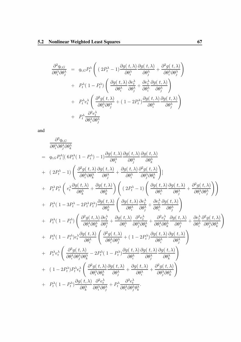
5.2 Nonlinear Weighted Least Squares 67
∂2qt,G∂θλi ∂θ
λj
= qt,GPλt
(( 2P λ
t − 1)∂g( t, λ)
∂θλi
∂g( t, λ)
∂θλj+∂2g( t, λ)
∂θλi ∂θλj
)
+ P λt ( 1− P λ
t )
(∂g( t, λ)
∂θλi
∂eλt∂θλj
+∂eλt∂θλi
∂g( t, λ)
∂θλj
)
+ P λt e
λt
(∂2g( t, λ)
∂θλi ∂θλj
+ ( 1− 2P λt )∂g( t, λ)
∂θλi
∂g( t, λ)
∂θλj
)
+ P λt
∂2eλt∂θλi ∂θ
λj
and
∂3qt,G∂θλi ∂θ
λj ∂θ
λk
= qt,GPλt [( 6P λ
t ( 1− P λt )− 1)
∂g( t, λ)
∂θλi
∂g( t, λ)
∂θλj
∂g( t, λ)
∂θλk
+ ( 2P λt − 1)
(∂2g( t, λ)
∂θλi ∂θλk
∂g( t, λ)
∂θλj+∂g( t, λ)
∂θλi
∂2g( t, λ)
∂θλj ∂θλk
)]
+ P λt P
λt
(eλt∂g( t, λ)
∂θλk+∂g( t, λ)
∂θλk
)(( 2P λ
t − 1)
(∂g( t, λ)
∂θλi
∂g( t, λ)
∂θλj+∂2g( t, λ)
∂θλi ∂θλj
))
+ P λt ( 1− 3P λ
t − 2P λt P
λt )∂g( t, λ)
∂θλk
(∂g( t, λ)
∂θλi
∂eλt∂θλj
+∂eλt∂θλi
∂g( t, λ)
∂θλj
)
+ P λt ( 1− P λ
t )
(∂2g( t, λ)
∂θλi ∂θλk
∂eλt∂θλj
+∂g( t, λ)
∂θλi
∂2eλt∂θλj ∂θ
λk
+∂2eλt∂θλi ∂θ
λk
∂g( t, λ)
∂θλj+∂eλt∂θλi
∂2g( t, λ)
∂θλj ∂θλk
)
+ P λt ( 1− P λ
t )eλt∂g( t, λ)
∂θλi
(∂2g( t, λ)
∂θλi ∂θλj
+ ( 1− 2P λt )∂g( t, λ)
∂θλi
∂g( t, λ)
∂θλj
)
+ P λt e
λt
(∂3g( t, λ)
∂θλi ∂θλj ∂θ
λk
− 2P λt ( 1− P λ
t )∂g( t, λ)
∂θλi
∂g( t, λ)
∂θλj
∂g( t, λ)
∂θλk
)
+ ( 1− 2P λt )P λ
t eλt
(∂2g( t, λ)
∂θλi ∂θλk
∂g( t, λ)
∂θλj+∂g( t, λ)
∂θλi+∂2g( t, λ)
∂θλj ∂θλk
)
+ P λt ( 1− P λ
t )∂g( t, λ)
∂θλk
∂2eλt∂θλi ∂θ
λj
+ P λt
∂3eλt∂θλi ∂θ
λj θ
λk
.

5.2 Nonlinear Weighted Least Squares 68
5.2.2 Consistency
As for the Nonlinear Least Squares problem, in order to solve this problem, weessentially want to find the solution of the “Weighted Least Squares Equations”:
∂Qn,G
∂θi= 0 ∀i = 1, · · · , s; s =
L∑
l=1
s( l). (5.24)
As previously, we would like to control the behavior of the Taylor expansion ofQn,G
around the optimal parameter given it exists. To do so, we have to state some setsof assumptions which are in a certain sense much stronger than what we have statedfor the least squares problem. This could be justifying why we started from the leastsquares problem, although one can consider the results for the least squares problemas corollaries of the much more general results which we are going to present in thecoming lines.
A. 5.16 1. Assume that τ ∈ N and p ∈ N; 1 ≤ p ≤ τ.
2. St,k is strictly stationary, α−mixing and independent ofXt,k, for each k =1, · · · , K.
A. 5.17 1. Zt,k, k = 1, · · · , K i.i.d. with mean 0.
2. ∃ Cj > 0 such that supk∈IK
E( |Zt,k|j | Xt = x) ≤ Cj <∞ for j = 1, · · · , 9.
3. mk(x), k = 1, · · · , K are continuous and ∃κ ≥ 0, ai ≥ 0 for i = 1 · · · , psuch that sup
k∈IK|mk(x)| ≤∑p
i=1 ai|xi|+ κ.
A. 5.18 1. Xt,k, k = 1, · · · , K are independent NLAR (p)-processes;
2. Xt,k is strictly stationary and α−mixing for each k ∈ IK.
3. E|Xt|4γ+1 <∞ for some γ > 2.
Remark 5.19 1. From the fact that Xt,k, k ∈ IK are independent, strictly sta-tionary stochastic processes and St,k is strictly stationary and independent ofXt,k for each k = 1, · · · , K, it follows that Xt is strictly stationary.
2. Xt satisfies an α−mixing condition with mixing coefficients for which the de-creasing rate is determined by the slowest decreasing rate of the mixing coef-ficients of Xt,k, k ∈ IK and of St,k.
The above remark is formalized in the following lemma.

5.2 Nonlinear Weighted Least Squares 69
Lemma 5.20 Let Xt,k, k ∈ IK be strictly stationary and independent stochas-tic processes, each satisfying an α−mixing condition. Also consider St,k to be astrictly stationary stochastic process independent of Xt,k for each k ∈ IK . More-over, assume St,k satisfies an α−mixing condition. Assume that ρt → 0 denotes asequence of upper bounds for the mixing coefficients of Xt,k, k ∈ IK , St. Then Xtis strictly stationary and satisfies an α−mixing condition with coefficient coefficientsbounded by (K + 1)ρt.
Proof: It is that Xt is strictly stationary, let us concentrate on the proof of the sec-ond conclusion of the lemma. For that purpose, let us define the following:
F ( S)0 = σ( St,k, t ≤ 0) F ( S)
u+ = σ( St,k, t ≥ u)
Analogously we defineF ( Xk)
0 , F ( Xk)u+ , for each k and F ( X)
0 ,F ( X)u+ . It follows that
F ( X)0 ⊂
(∪kF ( Xk)
0
)∪ F ( S)
0
and
F ( X)u+ ⊂
(∪kF ( Xk)u+
)∪ F ( S)
u+ .
Using Theorem 1 p 4 from Doukhan [18], we can conclude that
α( F ( Y )0 ,F ( Y )
u+ ) ≤ α( F ( S)0 ,F ( S)
u+ ) +K∑
k=1
α( F ( Xk)0 ,F (Xk)
u+ )
from which it follows that Xt is α−mixing. Using Lemma B.2.2 page 175 inKroisandt [57], we conclude with the rate of convergence.
Remark 5.21 By means of the Geometric Ergodic Theory we have established theasymptotic stationarity of Xt under weak assumptions. Hence all the assumptionof the previous lemma can be considered as technical tools to achieve the results onthe asymptotic properties of the parameter estimates in the weighted least squaresapproach.
A. 5.22 For each network nl, l = 1, · · · , L the activation functions ψ are boundedC3 with bounded derivatives.
A. 5.23 Assume that QG attains it unique global minimum (θ(1)0 , · · · , θ(L)
0 ) which isan interior point of ΘG (compact subspace ofRs) and also assume∇2QG(θ
(1)0 , · · · , θ(L)
0 )is positive definite.

5.2 Nonlinear Weighted Least Squares 70
Lemma 5.24 Consider assumptions A.5.16-A.5.22 to hold. Then, it follows that
E∣∣∣elt(θ(1)
0 , · · · , θ(L)0 )∣∣∣4
<∞ ∀l = 1, · · · , L; (5.25)
E∣∣∣∣∂g(t, l)
∂θi(θ
(1)0 , · · · , θ(L)
0 )
∣∣∣∣4
<∞ ∀ i = 1, · · · , s (5.26)
E∣∣∣∣∂2g(t, l)
∂θi∂θj(θ
(1)0 , · · · , θ(L)
0 )
∣∣∣∣3
<∞ ∀ i, j = 1, · · · , s (5.27)
E∣∣∣∣∂3g(t, l)
∂θi∂θj∂θk(θ
(1)0 , · · · , θ(L)
0 )
∣∣∣∣2
<∞ ∀ i, j, k = 1, · · · s. (5.28)
Proof: By definition and using the triangular inequality together with the fact thatSt,k is bounded by 1 we have
∣∣Xt+1 − f(Xt, θl)∣∣ =
∣∣∣∣∣K∑
k=1
St,k(Xt+1 −mk(Xt))
+K∑
k=1
St,k(mk(Xt))− f(Xt, θl))
∣∣∣∣∣
≤K∑
k=1
|Xt+1 −mk(Xt)|+K∑
k=1
∣∣St,k(mk(Xt)− f(Xt, θl)∣∣ .
Hence
E(elt)4 = E
∣∣Xt+1 − f(Xt, θl)∣∣8
≤ E
(K∑
k=1
|Xt+1 −mk(Xt)|+K∑
k=1
|St,k(mk(Xt)− f(Xt, θl))|)8
≤ const.
(K∑
k=1
E|Xt+1 −mk(Xt)|8
+ EK∑
k=1
|St,k(mk(Xt)− f(Xt, θl))|8),
by using the fact that for a, b, τ ≥ 0, (a+ b)τ ≤ 2τ (aτ + bτ ) and the finiteness ofE|elt|4 it follows from assumptions A.5.16 to A.5.22.With a similar strategy we will find the necessary conditions to achieve the remain-ing part of the proof .By definition, we have
∂g(t, l)
∂θi= β
t+τ∑
j=t−τ
∂f
∂θi(Xj, θl)(Xj+1 − f(Xj, θl)). (5.29)
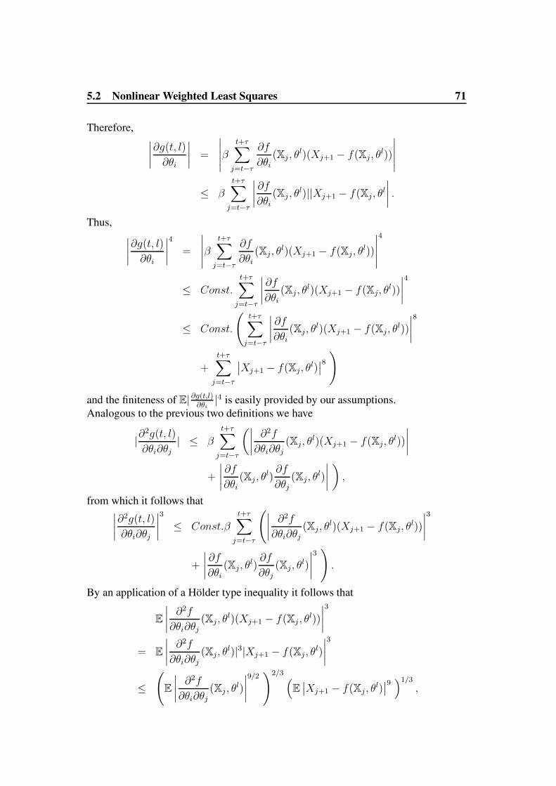
5.2 Nonlinear Weighted Least Squares 71
Therefore,∣∣∣∣∂g(t, l)
∂θi
∣∣∣∣ =
∣∣∣∣∣βt+τ∑
j=t−τ
∂f
∂θi(Xj, θl)(Xj+1 − f(Xj, θl))
∣∣∣∣∣
≤ βt+τ∑
j=t−τ
∣∣∣∣∂f
∂θi(Xj, θl)||Xj+1 − f(Xj, θl
∣∣∣∣ .
Thus,∣∣∣∣∂g(t, l)
∂θi
∣∣∣∣4
=
∣∣∣∣∣βt+τ∑
j=t−τ
∂f
∂θi(Xj, θl)(Xj+1 − f(Xj, θl))
∣∣∣∣∣
4
≤ Const.
t+τ∑
j=t−τ
∣∣∣∣∂f
∂θi(Xj, θl)(Xj+1 − f(Xj, θl))
∣∣∣∣4
≤ Const.
(t+τ∑
j=t−τ
∣∣∣∣∂f
∂θi(Xj, θl)(Xj+1 − f(Xj, θl))
∣∣∣∣8
+t+τ∑
j=t−τ
∣∣Xj+1 − f(Xj, θl)∣∣8)
and the finiteness of E|∂g(t,l)∂θi|4 is easily provided by our assumptions.
Analogous to the previous two definitions we have
|∂2g(t, l)
∂θi∂θj| ≤ β
t+τ∑
j=t−τ
(∣∣∣∣∂2f
∂θi∂θj(Xj, θl)(Xj+1 − f(Xj, θl))
∣∣∣∣
+
∣∣∣∣∂f
∂θi(Xj, θl)
∂f
∂θj(Xj, θl)
∣∣∣∣),
from which it follows that∣∣∣∣∂2g(t, l)
∂θi∂θj
∣∣∣∣3
≤ Const.βt+τ∑
j=t−τ
(∣∣∣∣∂2f
∂θi∂θj(Xj, θl)(Xj+1 − f(Xj, θl))
∣∣∣∣3
+
∣∣∣∣∂f
∂θi(Xj, θl)
∂f
∂θj(Xj, θl)
∣∣∣∣3).
By an application of a Holder type inequality it follows that
E∣∣∣∣∂2f
∂θi∂θj(Xj, θl)(Xj+1 − f(Xj, θl))
∣∣∣∣3
= E∣∣∣∣∂2f
∂θi∂θj(Xj, θl)|3|Xj+1 − f(Xj, θl)
∣∣∣∣3
≤(E∣∣∣∣∂2f
∂θi∂θj(Xj, θl)
∣∣∣∣9/2)2/3 (
E∣∣Xj+1 − f(Xj, θl)
∣∣9)1/3
,

5.2 Nonlinear Weighted Least Squares 72
from which we can deduce the finiteness of∣∣∣∣∂2g(t, l)
∂θi∂θj
∣∣∣∣3
.
In the final step of the proof of this lemma, we focus on
∣∣∣∣∂3g(t, l)
∂θi∂θjθk
∣∣∣∣ =
∣∣∣∣∣βt+τ∑
j=t−τ
(∂3f
∂θi∂θj∂θk(Xj, θl)(Xj+1 − f(Xj, θl))
− ∂2f
∂θi∂θj(Xj, θl)
∂f
∂θk(Xj, θl)
− ∂2f
∂θi∂θk(Xj, θl)
∂f
∂θj(Xj, θl)
− ∂2f
∂θj∂θk(Xj, θl)
∂f
∂θi(Xj, θl)
)∣∣∣∣ .
Hence, by similar arguments as those previously used,
∣∣∣∣∂3g(t, l)
∂θi∂θjθk
∣∣∣∣2
≤ const.t+τ∑
j=t−τ
(∣∣∣∣∂3f
∂θi∂θj∂θk(Xj, θl)(Xj+1 − f(Xj, θl))
∣∣∣∣2
+
∣∣∣∣∂2f
∂θi∂θj(Xj, θl)
∂f
∂θk(Xj, θl)
∣∣∣∣2
+
∣∣∣∣∂2f
∂θi∂θk(Xj, θl)
∂f
∂θj(Xj, θl)
∣∣∣∣2
+
∣∣∣∣∂2f
∂θj∂θk(Xj, θl)
∂f
∂θi(Xj, θl)
∣∣∣∣2)
Consequently
E∣∣∣∣∂3g(t, l)
∂θi∂θjθk
∣∣∣∣2
≤ const.
t+τ∑
j=t−τ
(E∣∣∣∣
∂3f
∂θi∂θj∂θk(Xj, θl)(Xj+1 − f(Xj, θl))
∣∣∣∣2
+E∣∣∣∣∂2f
∂θi∂θj(Xj, θl)
∂f
∂θk(Xj, θl)
∣∣∣∣2
+E∣∣∣∣∂2f
∂θi∂θk(Xj, θl)
∂f
∂θj(Xj, θl)
∣∣∣∣2
+ E∣∣∣∣∂2f
∂θj∂θk(Xj, θl)
∂f
∂θi(Xj, θl)
∣∣∣∣2)
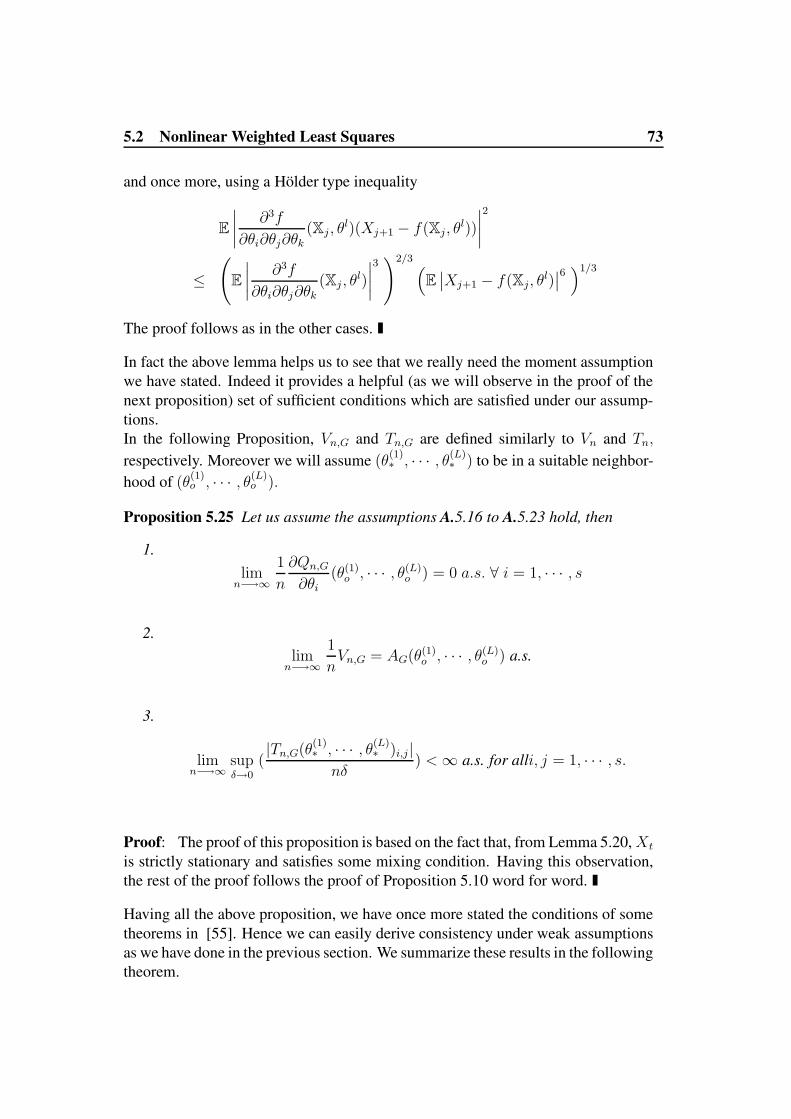
5.2 Nonlinear Weighted Least Squares 73
and once more, using a Holder type inequality
E∣∣∣∣
∂3f
∂θi∂θj∂θk(Xj, θl)(Xj+1 − f(Xj, θl))
∣∣∣∣2
≤(E∣∣∣∣
∂3f
∂θi∂θj∂θk(Xj, θl)
∣∣∣∣3)2/3 (
E∣∣Xj+1 − f(Xj, θl)
∣∣6)1/3
The proof follows as in the other cases.
In fact the above lemma helps us to see that we really need the moment assumptionwe have stated. Indeed it provides a helpful (as we will observe in the proof of thenext proposition) set of sufficient conditions which are satisfied under our assump-tions.In the following Proposition, Vn,G and Tn,G are defined similarly to Vn and Tn,
respectively. Moreover we will assume (θ(1)∗ , · · · , θ(L)
∗ ) to be in a suitable neighbor-hood of (θ
(1)o , · · · , θ(L)
o ).
Proposition 5.25 Let us assume the assumptions A.5.16 to A.5.23 hold, then
1.limn−→∞
1
n
∂Qn,G
∂θi(θ(1)o , · · · , θ(L)
o ) = 0 a.s. ∀ i = 1, · · · , s
2.limn−→∞
1
nVn,G = AG(θ(1)
o , · · · , θ(L)o ) a.s.
3.
limn−→∞
supδ→0
(|Tn,G(θ
(1)∗ , · · · , θ(L)
∗ )i,j|nδ
) <∞ a.s. for alli, j = 1, · · · , s.
Proof: The proof of this proposition is based on the fact that, from Lemma 5.20,Xt
is strictly stationary and satisfies some mixing condition. Having this observation,the rest of the proof follows the proof of Proposition 5.10 word for word.
Having all the above proposition, we have once more stated the conditions of sometheorems in [55]. Hence we can easily derive consistency under weak assumptionsas we have done in the previous section. We summarize these results in the followingtheorem.

5.2 Nonlinear Weighted Least Squares 74
Theorem 5.26 (Consistency under Weak Conditions)Under assumptions A.5.16 to A.5.27, there exists (θ
(1)n , · · · , θ(L)
n ) such that
(θ(1)n , · · · , θ(L)
n )→ (θ(1)0 , · · · , θ(L)
0 )a.s.
and for ε > 0, there is E with P(E) > 1 − ε and n0 such that on E for n >
n0, (θ(1)n , · · · , θ(L)
n ) satisfies the weighted least squares equation and Qn,G attains arelative minimum at (θ
(1)n , · · · , θ(L)
n ).
Proof: The proof of this theorem is similar to that of Theorem 5.7 given that allthe intermediate steps are achieved with the assumptions stated.
5.2.3 Asymptotic Normality
A. 5.27 supk∈IK
αXk(q) ≤ aq−ν for some a > 0 and ν > 1+ 12γ−1
, (IK = 1, · · · , K).
Proposition 5.28 Let us consider A.5.16 to A.5.27 to hold, then
n−1/2∇Qn,G(θ(1)0 , · · · , θ(L)
0 ) −→ N(
0, BG(θ(1)0 , · · · , θ(L)
0 )),
where
BG(θ(1)0 , · · · , θ(L)
0 )
= limn−→∞
E n−1∇Qn,G(θ(1)0 , · · · , θ(L)
0 )∇Qn,G(θ(1)0 , · · · , θ(L)
0 )′
= E∇qt,G(θ(1)0 , · · · , θ(L)
0 )∇qt,G(θ(1)0 , · · · , θ(L)
0 )′.
Proof: The proof is analogous to the proof of proposition 5.10.
A. 5.29 For each l = 1, · · · , L, f(x, θl), its first and second partial derivativeswith respect to (θ(1), · · · , θ(L)) are measurable w.r.t x, and uniformly continuous ina neighborhood of (θ
(1)0 , · · · , θ(L)
0 ) for every x.
Theorem 5.30 Let us consider A.5.16 to A.5.29 hold, then
n1/2((θ(1)n , · · · , θ(L)
n )− (θ(1)0 , · · · , θ(L)
0 ))→N(
0,ΣG(θ(1)0 , · · · , θ(L)
0 )),
where
ΣG = A−1G (θ
(1)0 , · · · , θ(L)
0 )BG(θ(1)0 , · · · , θ(L)
0 )A−1G (θ
(1)0 , · · · , θ(L)
0 )
AG(θ(1)0 , · · · , θ(L)
0 ) = limn−→∞
1
nVn,G
BG(θ0) = limn−→∞
E n−1∇Qn,G(θ(1)0 , · · · , θ(L)
0 )∇Qn,G(θ(1)0 , · · · , θ(L)
0 )′.

5.2 Nonlinear Weighted Least Squares 75
Proof: This proof follows the proof of Theorem 5.13.
In this section we have studied the consistency and the asymptotic normality of theparameter estimates for the non linear least squares problem and the weighted nonlinear least squares as well. Back to White [91] we have to observe that the expectedconsistency here just means convergence toward a local minimum of the criterionfunction. Moreover there is no guarantee to attain a global minimum. In general,asymptotic normality helps to set down test for the significance of the parameters.However, for the special case of the weighted least squares, it just means that theweights of the non divergent networks can achieve similar test of hypothesis on theirsignificance if the heat parameter is kept constant. Additionally this parameter needto be kept away from zero to make sure that the system satisfies some regularityassumptions.

76
6 Multivariate Weighted Least Squares for Change-point Analysis in Time Series Models
Unlike the previous chapter, the aim of the current chapter is to extend and prove thekey results established for univariate time series to higher dimensional time series.To achieve this goal we need to set some sufficient conditions and this is similarto what we have done in the previous chapter in two stages. In the first stage wewill find the asymptotic of the parameter estimates of a nonlinear Multivariate LeastSquares and in the second stage extend the results to the nonlinear MultivariateWeighted Least Squares.
6.1 Multivariate Least SquaresLet us assume that we have a nonlinear multivariate time series which can be writtenin the form
Xt+1 = m(Xt, · · · , Xt+1−p) + εt+1, t = 1, 2, · · · , (6.1)
where Xt and εt are d-dimensional vectors, Xt = (Xt, · · · , Xt+1−p) is a d × pmatrix andm is an unknown d-dimensional measurable function. Our objective is toapproximate this unknown function by a suitable multivariate feedforward network.Therefore, we shall need to minimize a Multivariate Least Squares Problem withunknown covariance matrix Σ of εt. Roughly speaking, the problem is in generalformulated as follows.The data are approximated by
Xt+1 = f(Xt, · · · , Xt+1−p, θ) + εt+1, t = 1, 2, · · · , (6.2)
when they were actually generated by
Xt+1 = m(Xt, · · · , Xt+1−p) + εt+1, t = 1, 2, · · · (6.3)
and one is supposed to solve the minimization problem
Qn(θ,Σ) =n−1∑
t=0
(Xt+1 − f(Xt, θ))′Σ−1(Xt+1 − f(Xt, θ)). (6.4)
The complexity of the problem can be regarded as that of solving a MultivariateLeast Squares Problem, where, in general, Σ−1 is unknown and not always easyto estimate. Nevertheless, if we were give a consistent estimate Σ, we could havesolved the following problem, i.e. minimize
Qn(θ, Σ) =
n−1∑
t=0
(Xt+1 − f(Xt, θ))′Σ−1(Xt+1 − f(Xt, θ)), (6.5)

6.1 Multivariate Least Squares 77
with Σ−1 being a known matrix. For sake of simplicity, in the following lines, wemake some (realistic) assumptions on Σ−1 to overcome the problem caused by itsestimation.On this way, if we assume Σ to be positive semi-definite( which should be the casefor any covariance matrix), from Linear algebra, one can construct the square rootΣ−1/2 of Σ−1 with the property Σ−1/2 ′ = Σ−1/2. By doing so the optimizationproblem can be reformulated in the following way:
Qn(θ,Σ) =
n−1∑
t=0
(Xt+1 − f(Xt, θ))′Σ−1/2Σ−1/2(Xt+1 − f(Xt, θ))
=
n−1∑
t=0
(Σ−1/2(Xt+1 − f(Xt, θ)))′(Σ−1/2(Xt+1 − f(Xt, θ)))
=
n−1∑
t=0
(Σ−1/2Xt+1 − Σ−1/2f(Xt, θ)))′(Σ−1/2Xt+1 − Σ−1/2f(Xt, θ)))
From this reformulation one can observe that a form similar to the Euclidean dis-tance appears and this is our motivation for formulating the problem as that of min-imizing the least squares Euclidean norm. For sake of simplicity, we limit ourselvesto the type of problem where the Σ ≡ Id (d-dimensional identity matrix), i.e. mini-mize,
Qn(θ) =n−1∑
t=0
(Xt+1 − f(Xt, θ))′(Xt+1 − f(Xt, θ)) (6.6)
=n−1∑
t=0
‖Xt+1 − f(Xt, θ)‖2. (6.7)
We can rewrite this as
Qn(θ) =
n−1∑
t=0
d∑
u=1
(Xt+1,u − fu(Xt,u, θu))2 (6.8)
=
n−1∑
t=0
Qt,M . (6.9)
By doing so we implicitly have to solve the minimization problem:
minθEQt,M = min
θQ(θ). (6.10)
As we have already done for the least squares and the weighted least squares in theone dimensional problem, we need to find a solution of:
∂Qn
∂θi(θ) = 0 for all i. (6.11)

6.1 Multivariate Least Squares 78
To achieve this goal, we need once more to control the asymptotic behavior of theTaylor expansion of Sn(θ) and hence the need of assumptions similar to those wehave stated up to now. Let us first define
Vn,S = ∇2Sn(θM)
Tn,S = ∇2Sn(θ∗M )− Vn,S
with θM being the unique global minimum of Q(θ) and θ∗M defined as θ∗ in the leastsquares problem relative to θM .Basically we have
∂Qt,M
∂θu,i= − ∂fu
∂θu,i(Xt,u, θu)(Xt+1,u − fu(Xt,u, θu)) (6.12)
and
∂2Qt,M
∂θu,i∂θh,j=
0 if h 6= u
− ∂2fu∂θu,i∂θu,j
(Xt,u, θu)(Xt+1,u − fu(Xt,u, θu))+ ∂fu∂θu,i
(Xt,u, θu) ∂fu∂θu,j
(Xt,u, θu) otherwise.
6.1.1 Consistency and Asymptotic Normality
Let us now state some basic assumptions on Xt and derive some consequences
A. 6.1 Assume that Xt is strictly stationary, α- mixing with mixing rate α(k) ≤ak−β for some a > 0 and some β > 1.
From this assumption, it follows that the marginals Xt,u, u = 1, · · · , d are alsostrictly stationary, α-mixing with mixing rate not greater than α(k).
A. 6.2 1. Assume thatXt is strictly stationary α-mixing and supu E|Xut |2γ <∞
for some γ > 2.
2. ∃ Cj > 0 such that supu E(|εut |j | Xut = x) ≤ Cj <∞ for j = 1, · · · , 4.
3. mk : Rp → R are continuous and ∃ κ ≥ 0 such that supk |mk(x)| ≤infk
∑pi=1 |xki |+ κ.
A. 6.3 Consider A.5.2 to hold for each network function fu.
A. 6.4 Q has its unique global minimum at θM which is an interior point of ΘM and∇2Q(ΘM) = AQ(ΘM) is positive definite.
Proposition 6.5 Let us consider A.6.1 to A.6.4 to hold. Then,
1. limn→∞1n∂Qn∂θi,u
(θM) = 0 a.s., for i = 1, · · · , l(u); u = 1, · · · , d.

6.2 Nonlinear Multivariate Weighted Least Squares 79
2. limn→∞1nVn,Q(θM )→ V a.s., where V is a positive definite matrix.
3.
limn→∞
supδ→0
( |Tn,Q(θ∗M )i,j|nδ
)<∞ a.s. for all i, j = 1, · · · , l(u), u = 1, · · · , d.
Proof: The proof is similar to that of Proposition 5.4.
A. 6.6 A.5.8 holds for Xt (compare Chapter 5, Section 5.1.2).
A. 6.7 For each u, fu(x, θ), its first, and second partial derivative w.r.t. θ, aremeasurable w.r.t. x and uniformly continuous in a neighborhood of θM for every x.
Theorem 6.8 Let A.6.1 to A.6.7 hold, then
n1/2(θn − θM)→N (0,Σ(θM)) ,
where
Σ = A−1(θM )B(θM)A−1(θM),
A =
(∂2EQt,M (θM )
∂θi∂θj
)
i,j
B(θM ) = E∇Qt,M (θM)∇Qt,M (θM)′.
Proof: A.6.1 to A.6.7 provide analogous of Theorem 5.7 and Proposition 5.10 withthe slight modification that one needs to use a Multivariate Central Limit Theoremfor stationary α-mixing processes(see, e.g. Billingsley [9]) and the Ergodic The-orem applied to stationary vector-valued processes. The proof follows similarly tothat of Theorem 5.13.
6.2 Nonlinear Multivariate Weighted Least SquaresLet Xtt≥0 be a multivariate nonlinear autoregressive process with switching
Xt =K∑
k=1
St,k(mk(Xt−1) + σk(Xt−1)εt,k) with St,k =
1 for Qt = k
0 else(6.13)
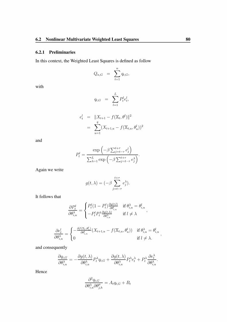
6.2 Nonlinear Multivariate Weighted Least Squares 80
6.2.1 Preliminaries
In this context, the Weighted Least Squares is defined as follow
Qn,G =
n∑
t=1
qt,G,
with
qt,G =L∑
l=1
P lt elt,
elt = ‖Xt+1 − f(Xt, θl)‖2
=
q∑
u=1
(Xt+1,u − f(Xt,u, θlu))2
and
P lt =
exp(−β∑t+τ
j=t−τ elj
)
∑Lλ=1 exp
(−β∑t+τ
j=t−τ eλj
) .
Again we write
g(t, λ) = (−βt+τ∑
j=t−τeλj ).
It follows that
∂P lt
∂θλi,u=
P lt (1− P l
t )∂g(t,l)
∂θli,uif θλi,u = θli,u
−P ltP
λt∂g(t,λ)
∂θλi,uif l 6= λ
,
∂elt∂θλi,u
=
−∂f(Xt,θlu)
∂θli,u(Xt+1,u − f(Xt,u, θlu)) if θλi,u = θli,u
0 if l 6= λ.,
and consequently
∂qt,G∂θλi,u
= −∂g(t, λ)
∂θλi,uP λt qt,G +
∂g(t, λ)
∂θλi,uP λt e
λt + P λ
t
∂eλt∂θλi,u
.
Hence
∂2qt,G∂θλi,u∂θ
µj,h
= Atqt,G +Bt

6.2 Nonlinear Multivariate Weighted Least Squares 81
with
At =
(P λt P
µt
∂g(t, λ)
∂θλi,u
∂g(t, µ)
∂θµj,h− ∂P λ
t
∂θµj,h
∂g(t, λ)
∂θλi,u− ∂2g(t, λ)
∂θλi,u∂θµj,h
)
and
Bt = −∂g(t, λ)
∂θλi,uP λt P
µt
(∂g(t, µ)
∂θµj,heµt +
∂eµt∂θµj,h
)+∂2g(t, λ)
∂θλi,u∂θµj,h
P λt e
λt
+∂g(t, λ)
∂θλi,u
(∂P λ
t
∂θµj,heλt + P λ
t
∂eλt∂θµj,h
)+∂P λ
t
∂θµj,h
∂eλt∂θλi,u
+ P λt
∂2eλt∂θλi,u∂θ
µj,h
.
Now let us consider different situations.
1. If λ = µ and u= h, it follows that
At = P λt (2P λ
t − 1)∂g(t, λ)
∂θλi,u
∂g(t, λ)
∂θλj,u− ∂2g(t, λ)
∂θλi,u∂θλj,u
and
Bt =∂g(t, λ)
∂θλi,uP λt
((1− P λ
t )∂2eλt∂θλj,u
− P λt
∂g(t, λ)
∂θλj,ueλt
)
+ P λt (1− P λ
t )∂g(t, λ)
∂θλj,u
(∂g(t, λ)
∂θλi,u+∂2eλt∂θλi,u
)
+ P λt
(∂2g(t, λ)
∂θλi,u∂θλj,u
eλt +∂2eλt
∂θλi,u∂θλj,u
)
2. If λ = µ and u 6= h, it follows that
At = P λt (2P λ
t − 1)∂g(t, λ)
∂θλi,u
∂g(t, λ)
∂θλj,h
and
Bt = −∂g(t, λ)
∂θλi,uP λt P
λt
(∂g(t, λ)
∂θλj,heλt +
∂2eλt∂θλi,u∂θ
λj,h
)+ P λ
t
∂g(t, λ)
∂θλi,u
∂eλt∂θλj,h
+ P λt (1− P λ
t )∂g(t, λ)
∂θλj,h
(∂g(t, λ)
∂θλi,u+
∂eλt∂θλi,u
).
6.2 Nonlinear Multivariate Weighted Least Squares 82
3. If λ 6= µ it follows that
At = 2P λt P
µt
∂g(t, λ)
∂θλi,u
∂g(t, µ)
∂θµj,h
and
Bt = −∂g(t, λ)
∂θλi,uP λt P
µt
(∂g(t, µ)
∂θµj,heµt +
∂eµt∂θµj,h
)−
+∂g(t, λ)
∂θλi,uP λt P
µt
∂g(t, µ)
∂θµj,heλt −
∂g(t, µ)
∂θµj,hP λt P
µt
∂eλt∂θµj,h
.
Finally,
∂3qt,G∂θλi,u∂θ
µj,hθ
γk,z
= qt,G
(∂At∂θγk,z
− ∂g(t, γ)
∂θγk,zP γt
)
+ AtPγt
(∂g(t, γ)
∂θγk,zeγt +
∂eγt∂θγk,z
)+
∂Bt
∂θγk,z.
6.2.2 Consistency and Asymptotic Normality
Let us state some assumptions.
A. 6.9 A. 5.16 holds (compare Chapter 5, Section 5.2.2).
A. 6.10 1. Zt,k, k = 1, · · · , K are i.i.d. with mean 0,
2. ∃ Cj > 0 such that supk∈IK ,h∈Id
E(|Zt,k,h|j|Xt = x) ≤ Cj <∞.
3. mk,h(X), k ∈ IK, h ∈ Id are continuous and ∃κ ≥ 0, ai ≥ 0, i ∈ Ip such thatsup
k∈IK ,h∈Id|mk,h(x)| ≤ inf
k∈IK ,h∈Id
∑pi=1 ai|xi,k,h|+ κ.
A. 6.11 1. Xt,k, k = 1, · · · , K are independent multivariate NLAR(p)-processes.
2. Xt,k is strictly stationary and α−mixing for each k ∈ IK.
3. supk∈IK ,h∈Id
E|Xt,k,h|4γ+1 <∞ for some γ > 2.
A. 6.12 A. 5.2 (compare Chapter 5, Section 5.1.2) holds for each network functionfk,h, k ∈ IK, h ∈ Id.
6.2 Nonlinear Multivariate Weighted Least Squares 83
A. 6.13 S has its unique global minimum at θG which is an interior point of ΘG and∇2Q(θg) = AQG(ΘG) is positive definite.
Let us define
Vn,QG = ∇2Qn,G(θG)
Tn,QG = ∇2Qn,G(θ∗G)− Vn,QG,with θG being the unique global minimum of QG(θ) and θ∗G defined as θ∗ in the leastsquares problem relative to θG.The two results are the analogous of proposition and theorem established earlier andthe proofs follow their proofs, assuming that all intermediate states are obviouslyproved given our set of assumptions. Therefore, we will skip their proofs here.
Proposition 6.14 Given A.6.9 to A.6.11 hold, it follows that
1. limn→∞1n
∂Qn,G∂θi,u
(θG) = 0 a.s., for i = 1, · · · , l(u); u = 1, · · · , d,
2. limn→∞1nVn,QG(θG)→ V a.s. where V is a positive definite matrix and
3.
limn→∞
supδ→0
( |Tn,QG(θ∗G)i,j|nδ
)<∞ a.s. for all i, j = 1, · · · , l(u), u = 1, · · · , d.
The Asymptotic normality of the parameter estimate is formulated as follows,
Theorem 6.15 Let A.6.9 to A.6.13 hold, then
n1/2(θn − θG)→N (0,Σ(θG)) ,
where
Σ = A−1(θG)B(θG)A−1(θG),
A =
(∂2Eqt,G(θG)
∂θi∂θj
)
i,j
B(θG) = E∇qt,G(θG)∇qt,G(θG)′.
Beside all these theoretical considerations, the question we need to answer is how tosolve the problem numerically? For this aim, we have to relax our assumption anduse the result by White [91]. In fact, under some special conditions, he proves theconvergence and asymptotic normality of Backpropagation for this type of networkfunction.As for the Least Squares Problem, we have spoken about the existence of a consis-tent sequence of estimates for the Weighted Least Squares Problem. But we havenever said how we can compute these estimates. In the coming section, based onthe work done by White, we will relax some of our assumptions and prove thatBack-propagation can help to solve this problem from a numerical point of view.

84
7 A Numerical Procedure: BackpropagationHere, we are concerned with the general problem of finding algorithm that allows toretrieve the parameters of a model given the cost function that we have to optimize.For this purpose, we will present a version of the stochastic approximation algorithmthat helps us to numerically solve the problem of weighted least square as presentedin the previous chapter. Basically the stochastic approximation theory goes back toRobbins and Monro, but here we shall follow the approach by White [88], who usedthe results by Ljung to derive convergence of gradient descent in Neural Networkscontext.In this chapter we strengthen our model assumptions, and therefore, consider a re-gression model instead of autoregression model, i.e.
Yt = m(Xt) + σ(Xt)εt (7.1)
with i.i.d. Xt, εt instead of the model defined in equation 5.1. Then, the Zt =(Yt,X′t)′ are i.i.d. random vectors. We want to simplify our considerations, as ourmain goal is to show that Backpropagation also work for mixture models. We aresure that the results can be extended to the α-mixing time series case 5.1 as forthe case K = L = 1 for which White [88] has already shown the convergenceof Backpropagation. Moreover, to avoid lengthy technical expositions, we restrictourselves in this chapter to bounded i.i.d. random variables.Let us then recall the conditions in [88] and derive the result for the Weighted LeastSquares Problem in the regression situation.
7.1 Convergence of BackpropagationBefore we present the convergence theorem, let us state a proposition which can beconsidered as the base of the proof of the convergence of the numerical procedure.Let us first recall some useful definitions.
Definition 7.1.1 For Φ ⊆ Rd and θn a sequence of vectors, θn → Φ means that
infθ∈Φ|θ − θn| → 0 as n→∞. (7.2)
One will write θn →∞ if |θn| =∞.Finally, for θ∗ ∈ Rd, and ε > 0, S∗ε ≡ θ : |θ − θ∗| < ε.All over this chapter we consider V = (V1, · · · , Vd)′
Proposition 7.1 (White, 1989)Let Zn be a sequence of i.i.d random v × 1 vectors such that |Zn| ≤ ∆ < ∞. Let
7.1 Convergence of Backpropagation 85
m : Rv × Rs −→ Rs be continuously differentiable on Rv × Rs and suppose thatfor each θ ∈ Rs
M(θ) ≡ E(m(Zn, θ))
exists. Let an ∈ R+ be a decreasing sequence such that∞∑
n=1
an =∞, limn→∞
sup(a−1n − a−1
n−1) <∞, and∞∑
n=1
adn <∞ for some d > 1.
Define the recursive procedure
θn = θn−1 + anm(Zn, θn−1)(n = 1, 2, · · · )
where θ0 ∈ Rs is arbitrary.
1. Suppose that there exists Q : Rs −→ R twice continuously differentiablesuch that ∇Q(θ)′M(θ) ≤ 0 for all θ ∈ Rs. Then either θn −→ Θ∗ ≡θ : ∇Q(θ)′M(θ) = 0 or θn −→∞ with probability one.
2. Suppose that θ∗ ∈ Rs is such that P[θn −→ S∗ε
]> 0 for all ε > 0. Then
M(θ∗) = 0. If, in addition, M is continuously differentiable in a neighbor-hood of θ∗ with ∇M∗ ≡ ∇M(θ∗) finite and
J∗ = E(m(Zn, θ∗)m(Zn, θ
∗)′)
is finite and positive definite, then the eigenvalues of ∇M ∗ all lie in the lefthalf-plane.
3. Suppose that the conditions of (1.) hold, that M(θ) = −∇Q(θ), that Q(θ)has isolated stationary points (strong local minimum) and that the conditionsof part (2.) hold for each θ∗ ∈ Θ∗ = θ : ∇Q(θ) = 0 . Then as n −→ ∞,either θn tends to a local minimum of Q(θ) with probability 1 or θn −→ ∞with probability 1.
Proof: This proposition is due to White [88], but essentially based on the workdone by Ljung [60]. Consequently, one should refer to the latter for a better under-standing of the proposition.
Having this proposition, we are now ready to present the asymptotic properties ofthe Backpropagation under our considerations. First, let us present the model weare concerned with. Let
QG(θ1, · · · , θl) = E(
L∑
l=1
P lneln) (7.3)
= Eg(Zn, θ1, · · · , θl). (7.4)

7.1 Convergence of Backpropagation 86
withelt = ( Yt − fl( Xt, θl))2
and
P lt =
exp
(−β
t+τ∑
j=t−τeln
)
L∑
λ=1
exp
(−β
t+τ∑
j=t−τeλj
)
as defined in Chapter 5. Keeping this equation in mind, let us give a set of sufficientconditions which may allows us to derive the consistency of Backpropagation.
A. 7.2 1. We have a training sequence Zt of i.i.d. random vectors satisfying|Zt| ≤ 4 <∞a.s.
2. For each network nl, we have the following:
f(X; θl) = Fl(νl0 +
H(l)∑
h=1
νlhψh(ωlh,0 +
p∑
i=1
Xiωlh,i)),
where Fl is defined on R and the activation functions
ψh : R→ I ≡ [0, 1]
are continuously differentiable of order 2 onR; θl = (νl, ωl) ∈ Rs(l), s(l) =H(l)(2 + p) + 1, H(l) is the number of hidden neurons in the network nl forl = 1, · · · , L.
3. an ∈ R+ is a decreasing sequence such that:
(a)∞∑
n=1
an =∞
(b) limn→∞ sup(a−1n − a−1
n−1) <∞
(c)∞∑
n=1
adn <∞ for some d > 1
Let make some comments on A. 7.2.Although A.7.2 -1. is somehow restrictive from the theoretical point of view( sinceit excludes the common Gaussian process), this assumption is reasonable for allpractical purposes because it does not make sense to work with processes that takevalues at infinity.

7.1 Convergence of Backpropagation 87
In the current work we choose the activation functions to be identical and definethem to be a type of sigmoid, for example the logistic function
φ(u) =1
1 + e−u. (7.5)
Conditions A.7.2-3a and A.7.2-3c are generalized versions of the conditions whichRobbins and Monro used in their pioneering work on stochastic approximation the-ory. Remark that A.7.2-3a is a necessary condition for the convergence of θn evenif there is no random error. Beside this, we can observe that an should not to betoo large, otherwise the random error will prevent the convergence. It turns outthat A.7.2-3c asymptotically damps the effect of experimental errors. AssumptionA.7.2-3b was first used by Ljung [60] for technical reason in the proof of his results.In general assumption A.7.2 holds for a very wide choice of an, the latter is usuallyconsidered as an = an−α(0 < α ≤ 1). The leading choice is with α = 1.
Lemma 7.3 Under the A. 7.2-1 and A. 7.2-2,
QG(θ1, · · · , θl) = E(
L∑
l=1
P lneln) (7.6)
= Eg(Zn, θ1, · · · , θl) (7.7)
is C2 on Ru w.r.t. θ, moreover
DkQG(θ1, · · · , θl) = EDk(L∑
l=1
P lneln) for k = 1, 2. (7.8)
where Dk are the k′th partial differentiations w.r.t. the parameters.
Proof: In this proof we essentially need to apply a theorem on the derivation ofparametric integrals, for example the theorem in Schmets [81] page 46.From A. 7.2-2, it follows that
∑Ll=1 P
lneln = g(z, θ) is twice continuously differ-
entiable on Ru × Rs, from which we can conclude that g(z, θ) is measurable withrespect to z and twice continuously differentiable w.r.t θ on Rs for each z.If we now consider a connected component of Rs, i.e. Rs itself and choose θc = 0 inthis connected component, then we obtain (by A. 7.2-1) that |g(z, θc)| is dominatedby an integrable function w.r.t to the probability measure. Similarly, if we also takeθc 6= 0(with the help of A. 7.2-1), it is easy to show that ‖∇g(z, θc)‖ is dominatedby an integrable function.Let us now consider a compact K ⊂ Rs. For θ ∈ K, continuity of ∇2g(z, θ) on thecompact subset(from A. 7.2.1) ofRu containing z implies that∇2g(z, θ) is bounded.Hence, ‖∇2g(z, θ)‖ is dominated by an integrable function and the proof of thelemma follows.
7.1 Convergence of Backpropagation 88
Theorem 7.4 Let us assume the conditions of A. 7.2 are satisfied, define the Back-propagation estimator
θn = θn−1 − an∇g(θn−1), n = 1, 2, · · · , (7.9)
where θ0 is arbitrary. Then either
θn → Θ∗ = θ : E(∇g(θ) = 0 w.p.1. or θn →∞ w.p.1..
If in addition, QG(θ) has isolated stationary points such that
J∗ = E(∇g(Zn, θ∗)′∇g(Zn, θ
∗))
is positive definite for each θ∗ ∈ Θ∗, then either θn converges to a local minimum ofQG(θ) w.p.1 or θn →∞.
Proof: For this proof we apply Lemma 7.3 and Proposition 7.1. Now Considerm(z, θ) = ∇g(z, θ),with g(z, θ) as defined in the proof of the previous lemma. A.7.2.1 ensures that Zn are i.i.d. uniformly bounded. From A. 7.2.2, ∇g(z, θ) iscontinuously differentiable and the lemma provides that for each θ ∈ Rs, M(θ) =E∇g(z, θ) exists. The conditions on an are provided by 7.2.3.If we take
Q(θ) = −EL∑
l=1
P lneln = −Eg(z, θ),
by Lemma 7.3, Q(θ) is twice continuously differentiable and
θ ∈ Rs,∇Q(θ)′M(θ) ≤ 0
for all θ ∈ Rs. Then the conclusion of Proposition 7.1.2 holds and therefore the firstpart of the theorem.By Lemma 7.3, ∇M(θ∗) is finite and by assumption J∗ is positive definite. Hence,the conditions of Proposition 7.1-2 hold. By Proposition 7.1-3, θn converges to alocal minimum of Q(θ).
7.1.1 Asymptotic Normality
In this section we essentially recall the assumptions by White [88], assumptions thathe uses to establish the asymptotic normality of the Backpropagation.
Proposition 7.5 Let the conditions of Proposition 7.1.(1, 2) hold and suppose that‖g(z, θ)‖ < ∆ < ∞ a.s. for all θ ∈ Rs. Let λ∗ be the maximum value of thereal part of the eigenvalues of ∇M(θ∗) and suppose that λ∗ < −1
2. Define J(θ) =
var[g(z, θ)] and suppose that J is continuous in a neighborhood of θ∗. Set J∗ =

7.1 Convergence of Backpropagation 89
J(θ∗) and an = 1n. Then the sequence of the random element Tn(a) of CRl [0, 1], with
sup norm defined by
Tn(a) = n−1/2S[na] + (na− [na])n−1/2(S[na]+1 − S[na]), a ∈ [0, 1]
( where Sn = (θn − θ∗)), converges to a Gaussian Markov process G with
G(a) = exp[(ln(a)(I+∇M(θ∗)]×∫
(0,a]
exp[−(ln(s)(I+∇M(θ∗)]dW (s), a ∈ (0, 1],
where W is a Brownian motion in Rl with
W (0) = 0,EW (1) = 0 and EW (1)W (1)′ = J(θ∗).
In particular,n1/2(θn − θ∗) −→ N (0, F ∗),
where
F ∗ =
∫
(0,1]
exp[−(ln(s)(I +∇M(θ∗)]J∗ exp[−(ln(s)(∇M(θ∗)′ + I)]ds
is the unique solution of the equation
(∇M(θ∗) + I/2)F ∗ + F ∗(∇M(θ∗)′ + I/2) = −J∗.
When ∇M(θ∗) is symmetric, F ∗ = PHP−1, where P is the orthogonal matrixsuch that PΩP−1 = −∇M(θ∗) with Ω the diagonal matrix containing the (real)eigenvalues (λ1, · · · , λl) of−∇M(θ∗) in the decreasing order andH the l×l matrixwith elements
Hij = (λi + λj − 1)K∗i,j(i, j = 1, · · · , l),where K∗ = P−1J∗P.
A. 7.6 Let A. 7.2.2 hold and let F , its derivatives and ψ be bounded.
Roughly speaking, this rules out the case(our case) in which F has to be regardedas the identity. However, taking
F (λ) =
λ for |λ| ≤ ∆
smooth and bounded for |λ| > ∆(7.10)
allows the approximation of the identity map. Additionally, since we assume Xt tobe bounded, the last approximation is always possible considering ∆ large enough,e.g. ∆ = CM0 where C > 1 and M0 the maximum value of the available data.
A. 7.7 For n = 1, 2, · · · , an = δn−1, δ > 0
7.1 Convergence of Backpropagation 90
Theorem 7.8 Let A. 7.2.1, A.7.6, A.7.7 be given and define θn as in equation (7.9).Suppose that θn → θ∗a.s., θ∗ an isolated stationary point of Q(θ) with J ∗ positivedefinite. Further, suppose that a > (2λ∗)−1, where λ∗ is the smallest eigenvalue of∇2Q∗ ≡ ∇2(θ∗). Then, Tn(a) as defined in the previous proposition converges indistribution to a Gaussian Markov process G with
G(a) = δ exp((ln a)[I − δ∇2QG(θast)]
∫
(0,a]
exp[(ln s)(δ∇2QG(θ∗)− I)]dW (s),
with W (0) = 0,E(W (1)) = 0, and E(W (1)W (1)′) = J(θ∗).In particular
n1/2(θn − θ∗) −→ N (0, F ∗) (7.11)
with F ∗ = PHP−1, where P is the orthogonal matrix such that PΩP−1 = ∇2Q∗,with Ω the diagonal matrix containing the eigenvalues (λ1, · · · , λl) of ∇2Q∗ in de-creasing order and H the s× s matrix with the elements
Hij = a2(aλi + aλj − 1)−1K∗ij i, j,= 1, · · · , s,
where K∗ = P−1J∗P.
Proof: The proof is essentially based on Proposition 7.5.Assumptions A.7.2-1, A.7.6 and A.7.7 suffice for the assumptions A.7.2-1to A.7.2-3 to hold. Thus, for the assumptions of Proposition 7.1.1. Since θ∗ is assumedto be isolated stationary point, the first condition of Proposition 7.1.2 holds. Theremaining conditions hold by a suitable use of Lemma 7.3 and given that J(θ∗) isassumed positive definite. Assumptions A.7.2.1 and A.7.6 ensure that ‖∇g(z, θ)‖is a.s. uniformly bounded for each θ ∈ Rs and the conditions on λ∗ are given byassumption. Finally the continuity of J in a neighborhood of θ∗ is provided byLemma 7.3.
The results presented in this section are proved under the main assumption of boundedi.i.d. random variables, assumptions that do not fit well to our case since nonlinearAutoregressive processes are dependent by nature.To make use of the dependence structure of the data and overcome the boundednessassumption, we can refer to the work done by Metivier and Priouret [69] where theymake a Markov assumption on the observed process and required strong assumptionlike, e.g., the existence of all moments for the Markov process and some regular-ity assumptions on the gradient of the cost function. Under their assumptions theyproved the convergence of the Backpropagation algorithm as defined in equation7.9.
91
8 Excursion to Tests in Changepoints DetectionIn this Chapter we recall the importance of tests for changepoint problem. We thenstate the general problem for our model and derive a first test for validating changein the dynamic of a parametric Nonlinear Autoregressive model. Here we considerthat the autoregressive and volatility functions are correctly specified by suitableFeedfoward Network with finite amount of hidden units, i.e. we are no longer in anonparametric setting.
8.1 GeneralitiesUnder the null hypothesis, that assuming there is no change in the dynamic of theobserved process, the model we defined in Chapter 2, equation 2.2, i.e.
Xt =
K∑
k=1
St,k(mk(Xt−1) + σk(Xt−1)εt,k) with St,k =
1 for k = Qt
0 otherwise,(8.1)
can be written asXt = m(α,Xt−1) + σ(β,Xt−1)εt (8.2)
with εt i.i.d. random variables and Xt−1 = (Xt−1, · · · , Xt−p). Under some regular-ity assumption on the autoregressive function m, the volatility function σ and somemixing condition on Xt one can prove the asymptotic normality of the parameterestimate. Instead of facing the not easy to solve problem of estimating the time ofchange by considering the autoregressive and volatility functions as well, we suggestto follow a stepwise approach. First we recommend to consider an autoregressivemodel without volatility function, in a next step one can consider a nonlinear ARCHmodel and finally one may focus on the more complex NAR-ARCH model.In the next section we will focus only on the first step and propose a test for estimat-ing the change in the model assuming there is only one change.
8.2 Test for Changes in Nonlinear Autoregressive ModelLet us consider under the null hypothesis the following model
Xt = f(Xt−1, θ) + εt (8.3)
where f is a given neural network.Now define the nonlinear least square(NLLS)
Qn(θ) =∑
t
((Xt − f(θ,Xt−1) )2 = min!
Let consider θn to be the least square estimate of θ0 the optimal parameter under thenull hypothesis of no change. By solving the Least Square Equations we obtain
∇Qn(θn) = 0. (8.4)

8.2 Test for Changes in Nonlinear Autoregressive Model 92
Providing the assumptions A.5.1 to A.5.9 of Chapter 5 one had proved that√n(θn − θ0) −→ N (0,Σ(θ)) (8.5)
Under the alternative we can rewrite our model with changes as following
Xt = f(θt,Xt−1) + εt. (8.6)
In general we shall make the following assumption on the residuals
A. 8.1 The εt are i.i.d. random variables with zero mean, nonzero variance σ2 andfinite moments E |εt|2+ν for some ν > 0.
For our purpose we will assume that under the alternative the time interval can besplit in two subinterval and for each interval θt has constant value. In other word weassume the existence of random integer 1 ≤ k < n such that for this k,
θ1 = θ2 = · · · = θk and θk+1 = · · · = θn 6= θk.
Following an idea by Huskova [52], we will use the M-estimator approach to derivethe test for detecting changepoint in this type of situation. In this light we refor-mulate the hypothesis, i.e. there is no change in the dynamic of the process as itfollows
H0 : θn,1 = θn,2 = · · · = θn,n (8.7)
and the alternative, that is there exists exactly one change in the dynamic of theprocess as
H1 : ∃ k, 1 ≤ k < n such thatθn,1 = θn,2 = · · · = θn,k and θn,k+1 = θn,k+2 = · · · = θn,n 6= θn,k.
Now, let us defineεt = Xt − f(θn,Xt−1)
it follows by equation 8.4 that∑
1≤t≤nεt = 0 (8.8)
that is∑
1≤t≤n(Xt − f(θn,Xt−1)) = 0 (8.9)
Let consider σ2n a consistent estimate of the variance of εt, and define for each
k = 1, · · · , n− 1 the partial sum
Sn,k =∑
1≤t≤kεt, (8.10)

8.2 Test for Changes in Nonlinear Autoregressive Model 93
and in turn
Tn = n−1/2 max1≤k<n
∣∣∣Sn,k∣∣∣ . (8.11)
Analogously, one can define
Sn,k =∑
1≤t≤kεt, (8.12)
Our goal is to prove that under the hypothesis
Tnσn−→ sup
0<s<1|B(s)|
where B(s) is a Brownian Bridge. Before we move forward in the definition of thetest, we first recall the definition of the Brownian Bridge.
Definition 8.2.1 A stochastic process B(t) 0 ≤ t ≤ 1 is called Brownian Bridge ifB(t) is a Gaussian process with B(0) = B(1) = 0,
EB(t) = 0 (8.13)
and
cov(B(t), B(s)) = s(1− t) 0 ≤ s ≤ t ≤ 1. (8.14)
Back to our goal, instead of doing the proof for Tnσ
we define
T ∗n = n−1/2 sup0<s<1
Sn,[ns]
where [ns] is the integer part of ns and carry out the proof for T ∗nσn, for which we can
now sketch the proof. By definition we have that
Sn,[ns] = Sn,[ns] − sSn,n ( by equation8.4) (8.15)
= Sn,[ns] − sSn,n − (Sn,[ns] − sSn,n) + (Sn,[ns] − sSn,n) (8.16)
= (Sn,[ns] − Sn,[ns]) + s(Sn,n − Sn,n) + (Sn,[ns] − sSn,n) (8.17)= T1,n + T2,n + T3,n (8.18)
where
T1,n = Sn,[ns] − Sn,[ns] (8.19)
T2,n = s(Sn,n − Sn,n) (8.20)

8.2 Test for Changes in Nonlinear Autoregressive Model 94
T3,n = (Sn,[ns] − sSn,n) (8.21)
By the weak convergence of the partial sum as used in Theorem 2.8.4 in [13], onehas
T3,n
n1/2σ−→ B(s) (8.22)
where B(s), 0 < s < 1 is a Brownian Bridge. For the remainder, we will applya Taylor expansion on f and use the limit distribution of the parameter estimate toconclude.Let us first apply a Taylor expansion on f around θ0. we then obtain
f(θn,Xt−1) = f(θ0,Xt−1) +∇f(θ0,Xt−1)(θn − θ0) + op (‖θn − θ0‖ ) .
Taking this into, that is by considering the asymptotic and neglecting the terms ofsmaller order we obtain
n−1/2∑
1≤t≤[ns]
(f(θn,Xt−1)− f(θ0,Xt−1)) (8.23)
= n−1/2∑
1≤t≤[ns]
∇f(θ0,Xt−1)(θn − θ0) (8.24)
∼=(n−1
∑
1≤t≤ns∇f(θ0,Xt−1)
)n1/2(θn − θ0) (8.25)
= s
(1
ns
∑
1≤t≤ns∇f(θ0,Xt−1)
)n1/2(θn − θ0) (8.26)
∝ s
(1
n
∑
1≤t≤n∇f(θ0,Xt−1)
)n1/2(θn − θ0). (8.27)
Hence, up to a constant factor T1,n
n1/2 and T2,n
n1/2 are asymptotically equivalent. There-
fore, if we prove that sup0<s<1
∣∣∣ T2,n
n1/2σ
∣∣∣ converges in probability to zero we can con-clude our claim. Indeed that is the case, we just need to notice by means of theasymptotic normality of θn and convergence of
1
n
∑
1≤t≤n∇f(θ0,Xt−1),
imply that∣∣∣∣Tn,2n1/2σ
∣∣∣∣ = op(1) (8.28)
and the claim follows.With all the above development we can now state the main theorem of this section,derive some of its consequences and propose a way to apply it.
8.2 Test for Changes in Nonlinear Autoregressive Model 95
Theorem 8.2 Under the assumptions A.5.1 to A.5.9 of Chapter 5, A.8.1 and thenull hypothesis it follows that
1√nσn
max1≤k<n
∣∣∣Sn,k∣∣∣ −→ sup
0<s<1|B(s)| (8.29)
where B(s), 0 < s < t is a Brownian Bridge and
σ2n =
1
n
∑
1≤t≤n(Xt − f(θn,Xt−1))2
To be complete with the proof, let us remark that we need to make use of the de-velopment that preceed the theorem. Additionally, we need to observe that σ2
n is aconsistent estimate of σ2
n and apply Slutsky’s Lemma to derive the result in equation8.29 from equation 8.22.Practically, this theorem can be used in the following way, reject the null hypothesisif
1√nσn
max1≤k<n
∣∣∣Sn,k∣∣∣ > U1−α (8.30)
where U1−α is the (1− α)-quantile of sup0<s<1 |B(s)|.In this chapter we develop a test assuming only one change in the dynamic of theprocess and as byproduct we are also able to derive an estimate time of change. Forthis time of change it will be of great interest to investigate its asymptotic property.Moreover, it will be interesting to extend the results of the current chapter to themodels with volatility component, that is nonlinear AR-ARCH model. Since it islimiting to assume only one change in dynamic of the process, it also important toextend the test to models with multiple changes.

96
9 Case StudiesIn this chapter we want to compare the theory of the Hidden Markov Driven modelspresented in Chapter 4 and the theory of the weighted least squares developed inChapter 5 to the reality. In this light, we first apply both approaches to computergenerated data, for which we know the exact hidden structure. Later we apply thehidden Markov Driven models approach to the forecasting of daily DAX values andthose of one of its main components, namely the BASF stock values.
9.1 Computer Generated DataIt is judicious for complex model classes to explore the behavior of the models in or-der to build up some intuition about well the models perform under well-known datastructure. Since GMAR-ARCH models contain an unsupervised part in learning, inthis section, we investigate whether the dynamics delivered by the models actuallycorrespond to the true ones. In other words we investigate whether the hidden statesare properly detected. For this purpose, we first consider a mixture of stationary firstorder autoregressive processes AR(1) to which we apply the weighted least squarestechniques that were presented in Chapter 5 and alternatively we generate data froma mixture of two nonlinear AR-ARCH(1) with hidden Markov state process and ap-ply the hidden Markov technique presented in Chapter 4 to these observations. Forboth cases the random residuals that we used were generated with MATLAB 6.5and the numerical computations were achieved by some self-implemented MAT-LAB routines.
9.1.1 Mixture of Stationary AR(1) and Weighted Least Squares Techniques
The data used in this section consist of two different stationary first order autoregres-sive processes Yt,1, Yt,2 and the hidden process St = (St,1, St,2) that determines thestates of the process. Having all these processes, we build up the following simplemixture model
Xt = St,1Yt,1 + St,2Yt,2, (9.1)
with
St,1 =
1 if t = 2kL + 1, · · · , (2k + 1)L, k ∈ N0 otherwise,
(9.2)
St,2 =
1 if t = (2k + 1)L+ 1, · · · , (2k + 2)L, k ∈ N0 otherwise,
(9.3)
where L is a given integer,Yt,1 = α1Xt−1 + εt
andYt,2 = α2Xt−1 + ζt

9.1 Computer Generated Data 97
for which εt, ζt are independent sequences of i.i.d. N (0, 1) random variables.We generate a sequence of 1200 realizations of the hidden process. This sequencedetermines which of the two processes is used in each time interval to generate therealization of the observed process. From the generated observations (sequence),we used the first 500 as the training set and the remainder as the validation set. Forthis simulation we consider the estimated instants of change and compare them withthe real time of change that we have considered for generating our process. We thenpresent the results of the simulation in the following picture.
0 200 400 600 800 1000 1200−10
−8
−6
−4
−2
0
2
4
6
8
10
Time
X t
Mixture of AR1(0.97) and AR1(−0.97) and Detection of Changes
Ori ChangesMARDet Changes
Figure 9.1: Detection of change: Mixture of AR(1)
The picture consists of a Mixture of AR processes(MAR) (the blue curve), thegenerated times of change that are represented by the vertical black lines and theestimated times of change represented by the jumps within the red curve.The observed process was generated by a superposition of two AR(1) processes gen-erated with autoregressive parameter α1 = 0.97 and α2 = −0.97. This superpositionconsists of taking the first 60 realizations of the mixture from the AR1(.97) and therealizations 61 to 120 from the AR1(−.97), in other words we consider L = 60 inthe model defined in Equation 9.1-9.2. By doing so iteratively we obtain our desiredprocess. For each underlying AR process the residuals were considered to be i.i.d.N (0, 1).The red curve estimates the presence in different states of the observed process andis also used to estimate the times of change. Indeed, the estimated times of changeare represented by the different jumps within the red curve. This means that when-ever a jump is observed, we estimate that we can move from one state to anotherone.

9.1 Computer Generated Data 98
A close analysis of the above results conclude that up to some small perturbations,the times of change are nicely estimated on the training set and the validation set aswell. Therefore, the weighted least squares techniques can be recommended for thesegmentation of the type of mixture we presented above.
9.1.2 GMAR-ARCH(1) and Hidden Markov Techniques
In the previous section, we work with a regular and deterministic unknown time ofchange, an assumption that in many situations may be very far from approximatingthe reality. Therefore, in this section, we consider a GMAR-ARCH(1), i.e. a modelof the form
Xt =
m1(Xt−1) + σ1(Xt−1)εt if St = 1
m2(Xt−1) + σ2(Xt−1)ζt if St = 0,(9.4)
where St ∈ 0, 1 have to be considered as a first order Markov Chain with transi-tion probability matrix A and the processes εt, ζt are independent sequences of i.i.d.N (0, 1) random variables.Under our setting, we consider that the dynamic of the Markov Chain is driven bythe transition probability matrix
A =
(0.985 0.0150.015 0.985
)
and we choose
m1(x) = αx + βe−γ(x−µ)2
m2(x) =eν−x
1 + eν−x
andσ1(x) =
√ω1 + a1x2 σ1(x) =
√ω2 + a2x2.
Where (α, β, γ, ν) ∈ R4, ω1 > 0, ω2 > 0 and a1 ≥ 0, a2 ≥ 0.Making use of the Markov structure, we generate 3000 realizations of the hiddenprocess St which helps us to know which dynamics was used at each time instantfor generating the observed process.Unlike the theory presented in Chapter 4, for the generated data under the abovemodel we assume the autoregressive and volatility functions can be suitably esti-mated by single layer feedforward networks. In this problem we are interested inthe estimation of the autoregressive functions (at each time instant) and the times ofchange as well (the hidden process).For this purpose, the usual technique for Neural Networks is taken into consider-ation, i.e. we split our data set into two subsets, namely the training set and thevalidation set. The first 1100 observations are used as training set and the remain-der are used as validation set. The results of the simulation are presented in thefollowing picture.

9.1 Computer Generated Data 99
0 500 1000 1500 2000 2500 3000
1
2
3
0 500 1000 1500 2000 2500 3000−1
0
1
2
0 500 1000 1500 2000 2500 3000−20
−10
0
10
20
Figure 9.2: Estimations under Computer Generated GMAR-ARCH(1) model
The picture above is composed of three subplots. The first subplot that containsthe black curve represents the estimated autoregressive part of the generated processat each time instant. The second subplot represents the generated hidden process andits estimates. In fact the green curve in this subplot represents St+2, that is a shiftedSt generated according to the model in equation 9.4 and the blue represents St + 1,where St is an estimate of St. The third subplot, i.e. the red curve represents thecomputer generated first order GMAR-ARCH data which are obtained via the gen-erated hidden process.For this estimation we consider exactly two states for the hidden Markov process asgenerated and use feedforward networks with 3 hidden layers for the autoregressiveand volatility functions as well. Additionally, the tanh-functions were chosen as ac-tivation functions for the estimation of the autoregressive functions and the logisticfunctions were considered for the estimation of the volatility functions.As one can observe, on the training set, the hidden process is well estimated up tothe perturbation that arises in a short period somewhere within the time span be-tween 500 and 700 where the phase is not properly estimated. Hence, in general thestatistical test for validating the changes will be of great help. Although there is nosuitable test at the moment for validating the changes, the estimated hidden processfits well the generated hidden Markov process on the validation set.
9.2 Forecast of Daily Stock Values and Market Strategy 100
9.2 Forecast of Daily Stock Values and Market StrategyThis section applies the Hidden Markov technique to the real-life data. The forecast-ing of the daily values of the DAX and those of BASF (one of its main components)is investigated. For this purpose, we first present the general situation and later onapply the model on each case with its particularities.
9.2.1 Model for Daily Stock Values
For the data we consider the daily stock values Yt and transform them via a shiftedlogarithm, i.e. we define
Xt = log Yt − logY1
for which we assume the following model
Xt =3∑
k=1
St,k(mk(Xt−1) + σk(Xt−1)εt)with St,k =
1 for k = Qt
0 otherwise(9.5)
where Qt is assumed to be a stationary Markov Chain with values in 1, 2, 3 andXt−1 = (Xt−1, · · · , Xt−p).As previously, we assume that each of the autoregressive and volatility functionscan be nicely approximated by a suitable feedforward network, that for sake of sim-plicity we choose to have the same amount of hidden neurons. Additionally, wechoose the order of the autoregressive without any particular assumption. Underthis consideration we are interested in the estimation of the autoregressive functionsand the estimation of the hidden process that we assume to be a M.C. as announcedpreviously. The estimate of the autoregressive function that we denote f : Rp −→ Ris used to build up a Market Strategy that we will define after an application of themodel in equation 9.5 to the forecast of transformed daily values of DAX and BASFrespectively. In general the tanh functions (they also return negative values) willaccount as activation functions for the estimation of the autoregressive function andthe logistic functions (they only return positive values) are used as activation func-tions for the estimation of the volatility functions.
Forecast of Transformed Daily DAX Values
The data used in this section are downloaded from the Internet (http://www.markt-daten.de/daten/daten.htm), the original data represent the daily observed values ofthe DAX. We transformed the data according to the procedure defined earlier, thatis considering Xt as defined in equation 9.5. We set p = 3 and make use of 5 hiddenneurons for each autoregressive and volatility function. Last but not least, we recallthat the hidden process is supposed to take values in 3 different states. Consideringthe first 1600 as training set we achieve the following results on the training set.
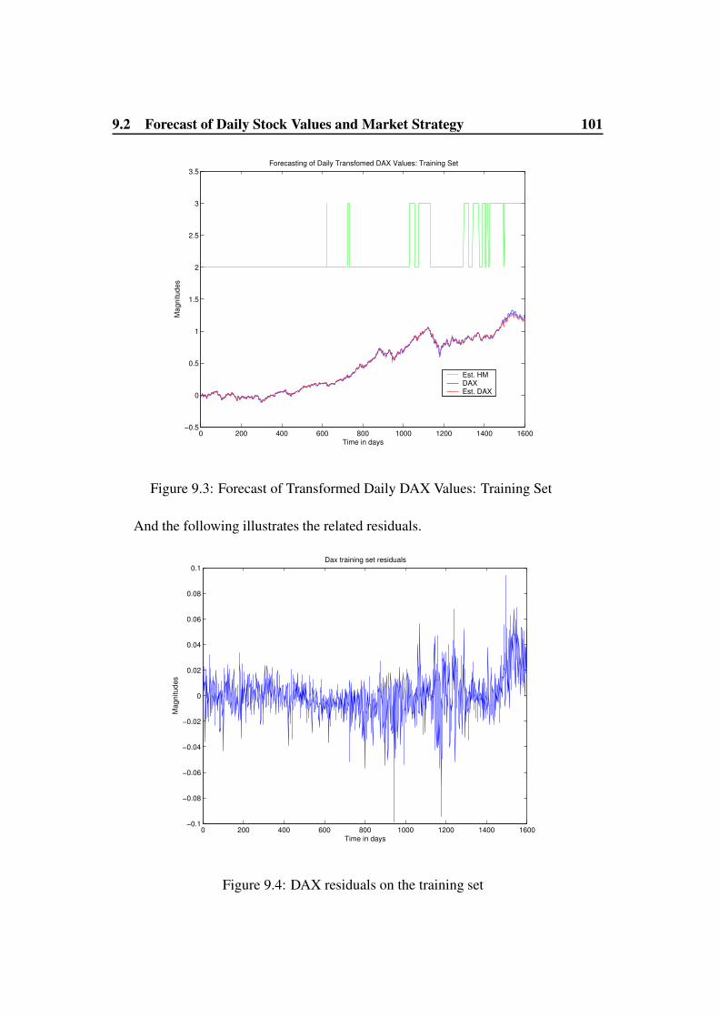
9.2 Forecast of Daily Stock Values and Market Strategy 101
0 200 400 600 800 1000 1200 1400 1600−0.5
0
0.5
1
1.5
2
2.5
3
3.5Forecasting of Daily Transfomed DAX Values: Training Set
Mag
nitu
des
Time in days
Est. HMDAXEst. DAX
Figure 9.3: Forecast of Transformed Daily DAX Values: Training Set
And the following illustrates the related residuals.
0 200 400 600 800 1000 1200 1400 1600−0.1
−0.08
−0.06
−0.04
−0.02
0
0.02
0.04
0.06
0.08
0.1
Mag
nitu
des
Time in days
Dax training set residuals
Figure 9.4: DAX residuals on the training set

9.2 Forecast of Daily Stock Values and Market Strategy 102
In Figure 9.3, the green curve represents the estimated Hidden Markov process,the blue curve the first 1600 observation of the transformed DAX values from the19th January 1984 to the 4th October 2004 and the red curve represents the estimatedautoregressive functions from the model in equation 9.5.From a first impression one has the feeling that the estimation procedure is in a cer-tain sense not stable enough, but a deeper analysis of the Figure 9.3, e.g. zoomingin the area of supposed instability delivers a completely different analysis. In fact,by zooming in on this area of apparent instability we observe that these perturba-tions account in general for changes over a short period, but in general not less than10 days. Moreover, these short changes correspond to very volatile periods on thefinancial market. These short periods of change that help us to be closer to the re-ality of financial market may help us to avoid big losses over theses periods or evenbetter may help us to achieve some gains in investment as it will be confirmed bythe market strategy that we will present in the next section.However, we have to remark that by assumption we have considered three states forthe hidden process, but now the results exhibit only two of them. This may looksurprising but the impression we have is that the procedure may be able to discardirrelevant dynamics.We can observe that the estimated autoregressive functions approximated the trans-formed daily data well. However, we need to point out the presence of a small trendat the end of the training set on the residual plot. All these observations are con-firmed by the validation set as the coming pictures illustrate.
1600 1800 2000 2200 2400 2600 28000
0.5
1
1.5
2
2.5
3
3.5Forecasting of Daily Transfomed DAX Values: Validation Set
Mag
nitu
des
Time in days
Est. HMDAXEst. DAX
Figure 9.5: Forecast of Transformed Daily DAX Values: Validation Set

9.2 Forecast of Daily Stock Values and Market Strategy 103
The related residuals plot is the following.
1600 1800 2000 2200 2400 2600 2800−0.15
−0.1
−0.05
0
0.05
0.1
Mag
nitu
des
Time in days
Dax validation set residuals
Figure 9.6: DAX residuals on the validation set
Unlike for the training set, in Figure 9.5 the green curve represents the estimatedHidden Markov process, the blue curve the remainder observations of the trans-formed DAX values from the 19th January 1984 to the 4th October 2004 and the redcurve represents the estimated autoregressive functions from the model in equation9.5 that we use to forecast the transformed daily DAX value, and in turn the dailyDAX values
9.2.2 Forecast of Transformed Daily Values of a DAX Component: BASF
The data used in this section, like those of the DAX observations, were downloadedfrom Internet (http://www.corporate.basf.com/en/investor/aktie/kurs.htm) and theyrepresent the transformed daily values of the BASF stock for the period from the 1st
July 1996 to the 12th October 2004.Once more we consider the transformed daily observations, in this case those ofdaily observed BASF values Yt that we define as it follows
Xt = log(Yt)− log(Y1)
and assume a model as defined in equation 9.5 for Xt. For this case we take p = 1and as previously, we assume that we can nicely approximate the autoregressive andvolatility functions by suitable Feedfoward Networks, networks that we now assumeto have 5 hidden neurons for each of the autoregressive and volatility functions. The

9.2 Forecast of Daily Stock Values and Market Strategy 104
results based on the training set (the first 1000 observations) are illustrated by thefollowing pictures.
0 100 200 300 400 500 600 700 800 900 1000−0.5
0
0.5
1
1.5
2
2.5Forecasting of Daily Transfomed BASF Values: Training Set
Mag
nitu
des
Time in days
Est. HMBASFEst. BASF
Figure 9.7: Forecast of Daily BASF Values: training Set
0 100 200 300 400 500 600 700 800 900 1000−0.1
−0.08
−0.06
−0.04
−0.02
0
0.02
0.04
0.06
0.08
Mag
nitu
des
Time in days
BASF training set residuals
Figure 9.8: BASF residuals on the training set
The previous figure represents the residual plot and in Figure 9.7 the green curve

9.2 Forecast of Daily Stock Values and Market Strategy 105
represents the estimated Hidden Markov driven process, the blue curve the obser-vations of the transformed BASF values and the red curve represents the estimatedautoregressive functions (at each time instant) from the model in equation 9.5.Again, we observe on the training set that only two networks seem to be useful forour purpose. This observation is not completely verified on the validation set sincethe third network occurs on the validation set. This occurrence of the third networkcan be analyzed in many different ways, but what seems to be plausible here is aspecial role devoted to that network. Indeed, the point of occurrence of this networkis located around the 11th of September 2001. Therefore, one can say that althoughthe third network is not present on the training it may be very useful for capturingextreme events.
1000 1200 1400 1600 1800 2000 2200 24000
0.5
1
1.5
2
2.5
3Forecasting of Daily Transfomed BASF Values: Validation Set
Mag
nitu
des
Time in days
Est. HMBASFEst. BASF
Figure 9.9: Forecast of Daily BASF Values: Validation Set
This extreme situation around the 11th September is also depicted on the resid-uals plot where a big and unusual variation is observed as Figure 9.10 illustrates.However, there is no trend on the residuals plot compare to the DAX residuals plot.A question arises at this point, why does the third network act in the case of BASFand not in that of the DAX. An explanation may be the fact that the DAX cap isless homogenous than BASF. Indeed, there are some variations in the compositionof the DAX cap over time, and therefore the difficulty in this case to predict extremeevents.
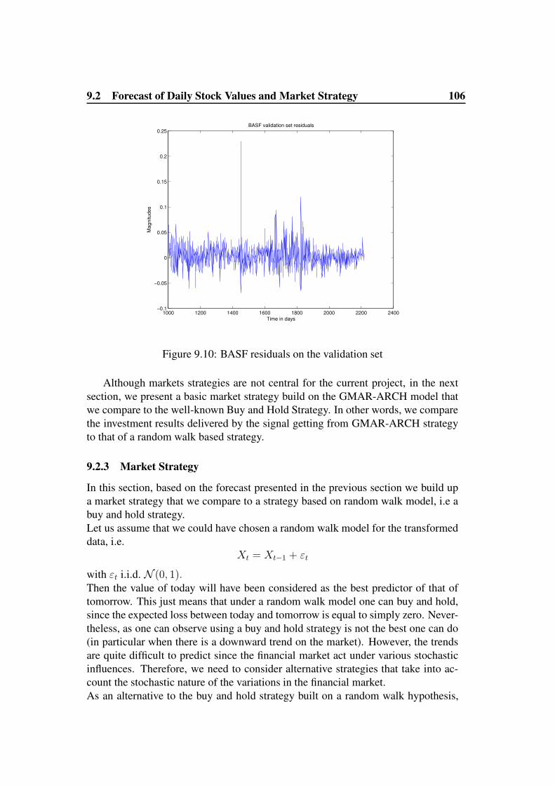
9.2 Forecast of Daily Stock Values and Market Strategy 106
1000 1200 1400 1600 1800 2000 2200 2400−0.1
−0.05
0
0.05
0.1
0.15
0.2
0.25
Mag
nitu
des
Time in days
BASF validation set residuals
Figure 9.10: BASF residuals on the validation set
Although markets strategies are not central for the current project, in the nextsection, we present a basic market strategy build on the GMAR-ARCH model thatwe compare to the well-known Buy and Hold Strategy. In other words, we comparethe investment results delivered by the signal getting from GMAR-ARCH strategyto that of a random walk based strategy.
9.2.3 Market Strategy
In this section, based on the forecast presented in the previous section we build upa market strategy that we compare to a strategy based on random walk model, i.e abuy and hold strategy.Let us assume that we could have chosen a random walk model for the transformeddata, i.e.
Xt = Xt−1 + εt
with εt i.i.d. N (0, 1).Then the value of today will have been considered as the best predictor of that oftomorrow. This just means that under a random walk model one can buy and hold,since the expected loss between today and tomorrow is equal to simply zero. Never-theless, as one can observe using a buy and hold strategy is not the best one can do(in particular when there is a downward trend on the market). However, the trendsare quite difficult to predict since the financial market act under various stochasticinfluences. Therefore, we need to consider alternative strategies that take into ac-count the stochastic nature of the variations in the financial market.As an alternative to the buy and hold strategy built on a random walk hypothesis,
9.2 Forecast of Daily Stock Values and Market Strategy 107
based on the GMAR-ARCH model we proposed a simple strategy that is based onthe following simple idea:If there is a positive signal (what we will define next), one should buy the stock inconsideration with all the money available at that time in the saving account or holdthe stock one already has in possession at that time. Conversely, if there is a neg-ative signal one should not buy any stock, moreover one should sell all the stocksin possession at that time or keep the money in the saving account if one does notpossess any stock at that time.For this strategy we make the following assumption
A. 9.1 (Main Assumption)There is no transaction cost and there is no interest rate on saving accounts.
Under the above hypothesis, let us now consider Yt to be the observed process, e.g.the daily observed DAX values and Xt the transformed DAX values. Under ourconsiderations,
Xt = log(Yt)− log(Y1)
and Xt follows a GMAR-ARCH model for which we assume that the autoregressivefunctions can nicely be estimated at each time point by suitable neural networksthat we denote f(Xt−1, · · · , Xt−p). The announced trading strategy is then built asfollows.Given an initial value of the observed series Y0 and an initial wealth G0 that we areto invest in a given stock we need to define the wealth process Gt, that is the amountof money related to the given stock given the initial wealth. The wealth processis built on the auxiliary process Amt which is the corresponding amount of stockgiven the signal.At each time instant t we compute f(Xt, · · · , Xt+1−p)−Xt (the announced signal)and define
Amt =
GtYt
if f(Xt, · · · , Xt+1−p)−Xt > 0
0 otherwise
and the decision for the next time is made as it follows
Gt+1 =
AmtYt+1 if Amt > 0
Gt if Amt = 0.
This trading strategy was applied on the validation set for the DAX and BASF valueswith initial wealth of 1000 units. Moreover the wealth processes generated in bothcases are compared to those generated by the Buy and Hold strategy. The results arepresented in the coming pictures where in both cases the blue curve represents thewealth process generated by the Hidden Markov based strategy and the red curveis the wealth process as delivered by the Buy and Hold strategy. In both situations,the hidden Markov based strategy performs better than the Buy and Hold strategy.
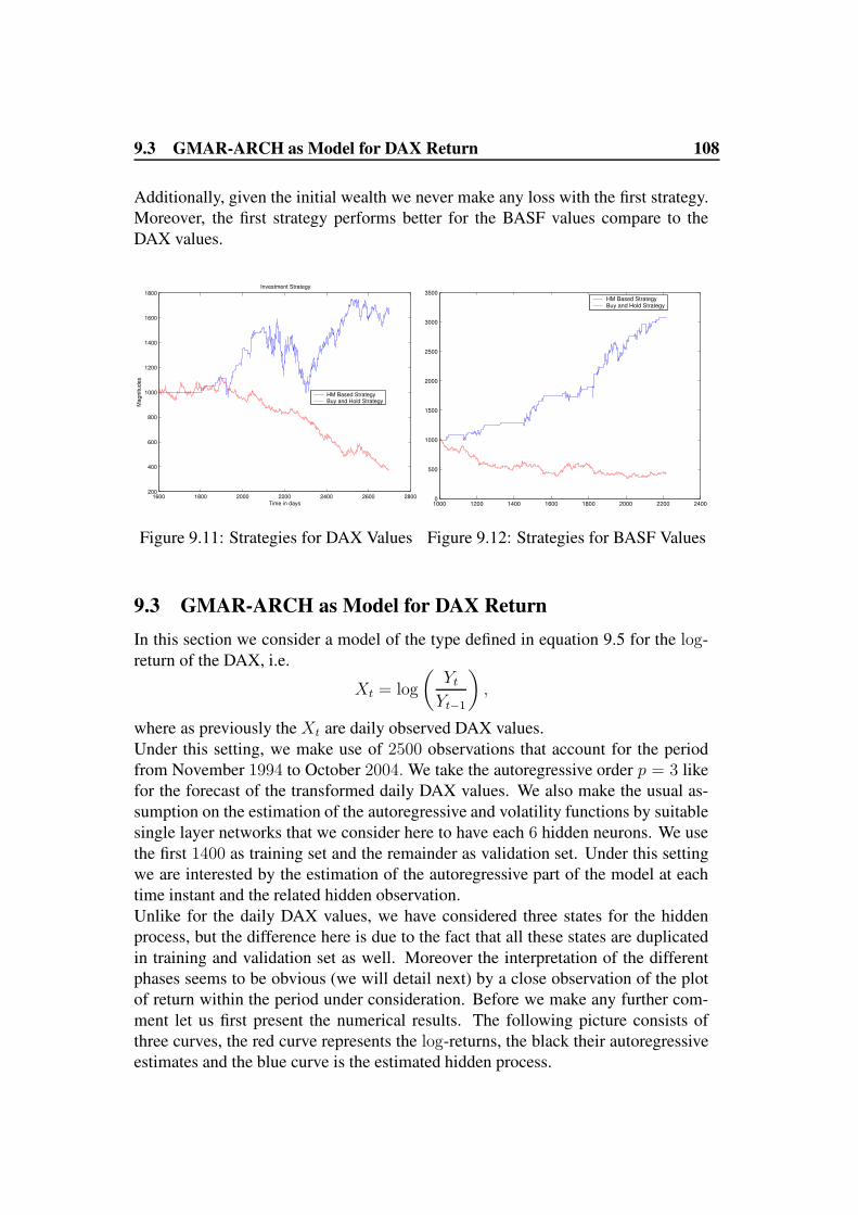
9.3 GMAR-ARCH as Model for DAX Return 108
Additionally, given the initial wealth we never make any loss with the first strategy.Moreover, the first strategy performs better for the BASF values compare to theDAX values.
1600 1800 2000 2200 2400 2600 2800200
400
600
800
1000
1200
1400
1600
1800
Mag
nitu
des
Time in days
Investment Strategy
HM Based StrategyBuy and Hold Strategy
Figure 9.11: Strategies for DAX Values
1000 1200 1400 1600 1800 2000 2200 24000
500
1000
1500
2000
2500
3000
3500HM Based StrategyBuy and Hold Strategy
Figure 9.12: Strategies for BASF Values
9.3 GMAR-ARCH as Model for DAX ReturnIn this section we consider a model of the type defined in equation 9.5 for the log-return of the DAX, i.e.
Xt = log
(YtYt−1
),
where as previously the Xt are daily observed DAX values.Under this setting, we make use of 2500 observations that account for the periodfrom November 1994 to October 2004. We take the autoregressive order p = 3 likefor the forecast of the transformed daily DAX values. We also make the usual as-sumption on the estimation of the autoregressive and volatility functions by suitablesingle layer networks that we consider here to have each 6 hidden neurons. We usethe first 1400 as training set and the remainder as validation set. Under this settingwe are interested by the estimation of the autoregressive part of the model at eachtime instant and the related hidden observation.Unlike for the daily DAX values, we have considered three states for the hiddenprocess, but the difference here is due to the fact that all these states are duplicatedin training and validation set as well. Moreover the interpretation of the differentphases seems to be obvious (we will detail next) by a close observation of the plotof return within the period under consideration. Before we make any further com-ment let us first present the numerical results. The following picture consists ofthree curves, the red curve represents the log-returns, the black their autoregressiveestimates and the blue curve is the estimated hidden process.

9.3 GMAR-ARCH as Model for DAX Return 109
0 500 1000 1500 2000 2500
1
2
3
0 500 1000 1500 2000 2500−4
−2
0
2
4
0 500 1000 1500 2000 2500−10
−5
0
5
10
Figure 9.13: Return Estimation under GMAR-ARCH Model
The second network appears on the training set essentially at the beginning andon the validation right at the end, these two periods correspond to relative quietnesson the financial market. The first network seems to model the highly volatile phasesof the market as one can observe on the training and validation sets. Last but notleast, one can say that the third network models the phases intermediate phases be-tween the previous two phases.As one can observe, we can use the model to have a nice segmentation of the marketphases. However, we need to point out the problem we have with the estimation ofthe autoregressive part, in some numerical results, they were phases where the au-toregressive part was either always positive or always negative. Hence, the difficultyto use the autoregressive part in those situations.

110
10 Conclusion and OutlookIn this chapter we first summarize what has been done in this thesis, exhibit somefields of further investigation.
10.1 ConclusionIn current work, many problems of interest are addressed. We can mention the ex-tension of Nonlinear AR-ARCH models to the Generalize Mixture of AR-ARCHas defined in Chapter 2. For this model we provide some sufficient conditions toensure the asymptotic stability of the system, these conditions are fulfilled undervarious regularity assumptions.Given a special consideration of the autoregressive functions in this model, we es-tablish the universal approximation (consistency of function estimates) propertyof these functions by some parametric classes of functions and particularly someclasses of single layer Feedforward Networks. Further, considering both autoregres-sive and volatility functions, based on the hidden structure, we define a conditionallikelihood from which we derive a pseudo conditional log-likelihood under normal-ity assumption of the residuals and suitable approximation of the autoregressive andvolatility functions by single layer Feedforward Networks. For the pseudo condi-tional log-likelihood we prove the consistency of the parameter estimates and designa version of the well-known EM algorithm for the numerical extraction of the modelparameters.Beside this Hidden Markov Driven models, we also consider a nonlinear weightedleast squares approach for estimating the time of change and the autoregressive func-tions at each instant. Under analogous consideration as previously, i.e. we considerFeedfoward Networks as function estimates and prove the consistency and asymp-totic normality of the parameter estimates. Unfortunately, here we consider a mix-ture of independent stationary processes.Practically, one can say that the weighted least squares techniques and the HiddenMarkov Driven approach perform quite well as some case studies in Chapter 9 il-lustrate.Despite these successful applications of both approaches, it is important to mentionthe necessity of suitable statistical tests for validating the changes in the dynamicsof the observed process. In this light, we consider a special case (compare Chapter8) for which we build up a statistical test based on the moving sum technique intro-duced by Huskova [52].However, it is also important to mention that many questions, which merit furtherconsiderations, arise along the way and we will recall some of the most importantones in the next section. Additionally, we suggest an alternative formulation of thetype of problem solved in this thesis.
10.2 Outlook 111
10.2 OutlookAlong the chapters of this thesis we have mentioned several unsolved problems ofparticular importance. Among these problems, we can recall that of the the choiceof the order of the autoregressive and volatility functions. In other words we needto build some information criterion that may help for the order selection. The orderselection is also closely related to the choice of the order of the Hidden Markovprocess and the numberK of states of this hidden process. Additionally, consideringthe approximation of autoregressive and volatility by suitable neural networks, theproblem of the choice of the number of hidden neurons can be pointed out.Beside the problems related to information criterion, the problem of validating thechanges is crucial. This problem is partially addressed in Chapter 8 where a mixtureof nonlinear AR process with only one abrupt unknown change is considered. Thechallenge is to develop similar tests for Generalized Mixture of AR-ARCH modelsand to study the asymptotic property of the estimated time of change, which in thecase mentioned in Chapter 8 can be considered as a byproduct of the developed test.An interesting issue is also to extend all the above considerations to a multivariatetime series, in turn to a portfolio. Furthermore, one can focus on the hidden processfor which one can consider a long memory process compare to a first order MarkovChain. Under such consideration one will first like to extend our theory to cover thistype of situation or depending on the applications one may also solve the problemin terms of occupation time or number of jumps from one state to another one.

112
A An Introduction to Neural Networks
A.1 Preliminaries and Network DescriptionThe term Neural Network has evolved along the time and nowadays represents avery large class of models and learning methods. Its comparison to the human brainmakes it mysterious, however it is still too far from describing the reality of the hu-man brain. As it will be made clear in this chapter, a Neural Network can simplybe regarded as a parametric nonlinear statistical model, much like projection pursuitamong others.Typically a Neural Network has a graphical representation as in figureA.1 where the(X1, · · · , Xp) represent the Input variables, the (Y1, · · · , Xq) the Output variablesand(in between) the (Z1, · · · , ZH) represents the Hidden layers. The latter are socalled because there are not directly observable.
Input Layer Hidden Layer Output Layer
PSfrag replacementsX1
X2
X3
Xp
.........
F1
F2
Fq
Z1
Z1
Zh
Y1
Y2
Yq
Input Layer
Figure A.1: Feedfoward Network
In this chapter we focus on the most widely-used class of Neural Network,namely on the class of single Layer Feedfoward Network. For sake of simplicitywe consider q = 1, i.e., we consider that the output to represent a single variable.Nevertheless one can refer to the book by Haykin [46] for a more general introduc-tion into this area or to the book by Anders [2] for an introduction and applicationto the Credit Scoring.Under our setting we have to recall that (as usual), the hidden features Zh are de-rived from linear combinations of the input variables and the target Y is defined as

A.1 Preliminaries and Network Description 113
a function of the linear combinations of the Zh, that is
Zh = ϕh(α0,h + α1,hX1 + · · ·+ αp,hXp) (A.1)= ϕh(α0,h + α′hX) for h = 1, · · · , H
and
Y = FH(ν0 + ν1Z1 + · · ·+ νHZH) = ν0 +
H∑
h=1
νhZh. (A.2)
The functions ϕh, which may be different for different values of h are called acti-vation functions and often taken to be the type of sigmoid with the most popularchoice being the sigmoid function, i.e.
ϕh(x) =1
1 + e−x
and FH is a given function for which the identity function or the truncated identityfunction can always be considered to solve regression problems.
A.1.1 Some Examples of Activation Functions
In Neural Network literature one can find various type of activation functions, inthis section we recall few of them. For more detail knowledge on this issue one canrefer to the literature mentioned previously in this chapter.
1. Linear functions of the form ϕ(x) = αx(for some α ≥ 0). Consideringthis activation function for every hidden unit, the entire system collapses toa linear model. Therefore, one can consider Neural Networks as nonlineargeneralization of linear models, e.g., for regression problems.
2. Threshold function that is defined as
f(x) =
1 if x > a
0 otherwise(A.3)
where a is given bound. The next picture represents such function for a = 1.
−5 −4 −3 −2 −1 0 1 2 3 4 5
0
0.1
0.2
0.3
0.4
0.5
0.6
0.7
0.8
0.9
1
Figure A.2: Threshold Activation function

A.1 Preliminaries and Network Description 114
3. Piecewise linear functions that for some α > 0 are defined as
f(x) =
0 if x < −α12( xα
+ 1) if − α ≤ x ≤ α
1 if α < x
In the following picture we give a graphical representation of such functionwith α = 1.
−5 −4 −3 −2 −1 0 1 2 3 4 5
0
0.1
0.2
0.3
0.4
0.5
0.6
0.7
0.8
0.9
1
Figure A.3: Piecewise Linear Activation Function
4. Sigmoid Function. This represents the most common activation used in theconstruction of neural networks. It is defined as a strictly increasing functionthat exhibits a graceful balance between linear and nonlinear behavior. Anexample is the well-known logistic function
ϕ(x) =1
1 + exp (ax), (A.4)
where a is the slope parameter of the sigmoid function. For the latter classof activation function, taking for example a big enough compare to 1 willaccount for a hard thresholding as one can observe from the following picture.
−5 −4 −3 −2 −1 0 1 2 3 4 5
0
0.1
0.2
0.3
0.4
0.5
0.6
0.7
0.8
0.9
1
Figure A.4: Type of Sigmoid Activation Functions
In the above picture we have different representations of ϕ(x) = 11+exp (−ax)
.For the black curve a = 1, for the red curve a = 15 and last but not the leastwe consider a = 0.2 for the blue curve.

A.2 Neural Networks in Practice 115
It may also be necessary to allow the activation function to take on negativevalues. In such situations the use of hyperbolic tangent functions, defined by
ϕ(x) = tanh (x) (A.5)
may be highly recommended.
A.2 Neural Networks in PracticeA.2.1 Least Squares
The Neural Networks have unknown parameters (usually called weights ) which wewant to estimate, i.e. we have to find the values of the weights that make the modelfit the data well. For this purpose we need to be given a training set
(Xt, Yt), t = 1, · · · , nwithXt ∈ Rp, Yt ∈ Rp and for the regression problem we can use the sum of squareerror
Q(θ) =
n∑
t=1
(Yt − fH(Xt))2 =
n∑
t=1
Qt,
where
fH(Xt) = ν0 +
H∑
h=1
νhϕ(α0,h + α′hXt).
For sake of simplicity we consider the same activation for all hidden units; θ ∈RH(p+2)+1 consists of
ν0, νh, h = 1, · · · , H; α0,h, αi,h, i = 1, · · · , p, h = 1, · · · , H.
A.2.2 Backpropagation
The standard approach used for the minimization of Q(θ) is a stochastic approxi-mation that we call Backpropagation in our context. Backpropagation is so popularbecause it is easy to implement. However, it can suffer from several drawbacks thatwe will discuss later.The algorithm can simply be defined as follows. Starting with a weight θ0 one de-rives the weight in the next step by the recursion formula
θn+1 = θn − γn∇Q(θn),
where ∇Q is the vector of first partial derivatives of Q with respect to θ and γn isthe learning that satisfies some technical conditions, namely
γn −→ 0 as n −→∞,∑
n
γn =∞, and∑
n
γ2n <∞.
These conditions are satisfied for γn = 1n. Therefore, one can observe that Back-
propagation is a form of the stochastic gradient algorithm due to Robbins and Monro(1951).

A.3 Some Technical Remarks 116
Drawback of Backpropagation and Alternative Solutions
The main drawback of backpropagation is the fact that if the dimension of the pa-rameter is very high or the size of the training set is large enough the algorithm maybecome very slow and for this reason one would rather rely on second order tech-niques such as the Newton algorithm. But the latter algorithm is not the best onecan use, in the sense that in this case one will need an explicit computation of thematrix of second derivatives, which can be very large in this case . To overcome thisproblem one can use a conjugated gradient algorithm or a variable metric method,both approaches avoid explicit computation of the Hessian while providing fasterconvergence.
A.3 Some Technical RemarksA.3.1 Input
It is recommended to scale all the input around their sample mean and variance. Thiswill ensure that all input are treated almost equally and may improve the qualityof the results. In this situation we can easily take our starting value as uniformlydistributed on the interval [−a, a]. However, if we choose a to be too close to zero,this just means that we allow our model to start into a linear model because inthis case the neural network collapses into a nearly linear model. As the weightsincrease, we go back to a nonlinear estimation problem.
A.3.2 Local minima
The objective functions are by nature non convex, therefore possessing many localminima. As a consequence, the final result obtained is always dependent on thechoice of starting value. Therefore we will at least try a number of random startingpoints and choose the solution given the best solution to our problem. Since weare in a nonlinear setting this approach is better than averaging over all the finalsolutions.
A.3.3 Number of Hidden Neurons
Roughly speaking it is better to have too many neurons than too few. With toofew hidden neurons, the model might not provide enough flexibility to capture allnonlinear aspects in the data. With too many neurons, extra weights can be set tozero by an appropriate regularization.
REFERENCES 117
References[1] Takeshi Amemiya. Advanced Econometrics . Havard University Press, USA,
1985.
[2] Ulrich Anders. Statistische Neuronale Netze. Verlag Franz Vahlen GmbH,Munchen, 1997.
[3] Leonard E. Baum, Ted Petrie, Georges Soules, and Norman Weiss. A max-imization technique occurring in the statistical analysis of probabilistic func-tions of markov chains. The annals of mathematical statistics, 41(1), 1970.
[4] Herman J. Bierens. Robust methods and asymptotic theory. Lecture notes ineconomics and mathematical sytem 192, Springer Verlag, Berlin, 1981.
[5] Herman J. Bierens. Sample moments integrating normal kernel estimators ofdensity and regression functions. Sankhya, 45, 1983.
[6] Patrick Billingsley. Statistical Inference for Markov Processes . The universityof Chicago Press, USA, 1961.
[7] Patrick Billingsley. Ergodic Theory and Information . John Wiley & Sons,New York, USA, 1965.
[8] Patrick Billingsley. Convergence of Probability Measures. John Wiley &Sons, New York, USA, 1968.
[9] Patrick Billingsley. Probability and Measure . John Wiley & Sons, New York,Usa, 1986.
[10] Denis Bosq. Nonparametric Statistics for Stochastic Processes. Lecture Notesin Statistics 110. Springer-Verlag, Heidelberg, 1998.
[11] Leo Breiman. Probability . Addison-Wesley, USA, 1968.
[12] Peter J. Brocwell and R A. Davis. Time Series: Theory and Methods .Springer-Verlag, Germany, 1991.
[13] Myklos Csorgo and L Horvath. Limit Theorems in Change-point Analysis .John Willey & Sons, USA, 1997.
[14] Y. Davydov. Mixing conditions for markov chain. Theory of probability andits applications, 18(2), 1973.
[15] Georgi Dimitroff. Neural Network-based estimates for volatility. DiplomThesis, University of Kaiserslautern, 2001.

REFERENCES 118
[16] Jurgen Dippon. Asymptotic analysis of a learning method in neural network.Tagungsbericht Neuronale Netze in Ingenieuranwendungen (Hg. B. Krplin).ISD Univ. Stuttgart, 1996.
[17] Vincent Dortet-Bernadet. Choix de models pour chaıne de markov cachees.Academie des sciences, Editions scientifiques et medicales, 332, 1989.
[18] Paul Doukhan. Mixing - Properties and Examples. Lecture Notes in Statistics85. Springer-Verlag, Heidelberg, 1994.
[19] Paul Doukhan and M. Ghindes. Etude du processus Xn+1 = f(Xn) + en.C.R.A.S. Serie A, 290, 1980.
[20] Marie Duflo. Random Iterative Models. Springer-Verlag, Heidelberg, 1997.
[21] Ernst Eberlein and Murad S. Taqqu. Dependence in Probability and Statistics:A Survey of Recent Results . Birkhaeser, Germany, 1986.
[22] Robert J. Elliot, Lakhdar Aggoun, and John B. Moore. Hidden Markov Mod-els: Estimation and Control . Springer, USA, 1995.
[23] Robert F. Engle. Autoregressive conditional heteroscedasticity with estimatesof the variance of united kingdom inflation. Econometrica, 50, 1982.
[24] Vaclav Fabian. On asymptotic normality in stochastic approximation. TheAnnals of Mathematical Statistics, 39(4), 1968.
[25] Jurgen Franke. Nonlinear and nonparametric methods for analyzing financialtime series. In P. Kall and H.-J. Luethi, eds., Operation Research Proceedings98. Springer-Verlag, Heidelberg, 1998.
[26] Jurgen Franke. Portfolio management and market risk quantification usingneural networks. In W.S. Chan, W.K. Li and H. Tong, eds., Statistics and Fi-nance: An Interface. Imperial College Press, London , 2000.
[27] Jurgen Franke and Mabouba Diagne. Estimating market risk with neural net-works. working paper, 2001.
[28] Jurgen Franke, Wolfgang Hardle, and Christian Hafner. Statistik der Fi-nanzmarkte . Springer-Verlag, Heidelberg, 2001.
[29] Jurgen Franke and Gerald Kroisandt. Nonparametric changepoint detectionfor time series. To be published in Statistics and Decision, 2004.
[30] Jurgen Franke, Michael H. Neumann, and Jean P. Stockis. Bootstrapping non-parametric estimates of the volatility function. Report in Wirtschaftsmathe-matik , University of Kaiserslautern. To appear in Journal of Econometrics ,77, 2001.

REFERENCES 119
[31] Andrew M. Fraser and Alexis Dimitriadis. Forecasting probability densitiesby using hidden markov models with mixed states,. in A. Weigend and N.Gershenfeld(eds), Time Series Prediction: Forecasting the Future and Under-standing the Past, Addison Wesley, 1993.
[32] A. Ronald Gallant. Nonlinear Statistical Models. John Wiley & Sons, NewYork, 1987.
[33] Valentine Genon-Catalot, T Jeantheau, and C Laredo. Conditional likelihoodestimators for hidden markov models and stochastic volatility models. Scan-dinavian journal of statistics, 30, 2003.
[34] Walter R. Gilks, Sylvia Richardson, and David J. Spielgelhalter. MarkovChain Monte Carlo in Practice . Chapman and Hall, England, 1996.
[35] Michel Goossens, Frank Mittelbach, and Alexander Samarin. Der Latex-Begleiter. Addison Wesley, Munchen, Germany, 2000.
[36] Christian Gourieroux. ARCH Model and Financial Application. Springer-Verlag, New York, 1997.
[37] Ulf Grenander. Abstract inference. Wiley, New York, 1981.
[38] Dominique Guegan and Jean Diebolt. Probabilistic properties of the β-archmodel. Statistica Sinica, 4, 1994.
[39] Lszl Gyorfy, Michael Kohler, Adam Krzyzak, and Harro Walk. ADistribution-Free Theory of Nonparametric Regression . Springer-Verlag, Hei-delberg, 2002.
[40] Christian Hafner. Nonlinear Time Series Analysis with Applications to ForeignExchange Rate Volatility. Physica-Verlag, Heidelberg, 1998.
[41] James D. Hamilton. Rational expectations econometric analysis of changesin regimes: An investigation of the term structure of inetrest rate. Journal ofEconomic Dynamics and Control, 12, 1988.
[42] James D. Hamilton. A new approach to the economic analysis of nonstationarytime series and the business cycle. Econometrica, 57, 1989.
[43] James D. Hamilton. Time Series Analysis. Princeton University Press, Prince-ton, 1994.
[44] Edward J. Hannan. Multiple time series. Wiley, New York, 1970.
[45] Trevor Hastie, Robert Tibshirani, and Jerome Friedmaan. The Elements ofStatistical Learning: Data Mining, Inference, and Prediction. Springer Verlag,New York, Berlin, Heidelberg, 2001.
REFERENCES 120
[46] Simon Haykin. Neural Networks: A Comprehensive Foundation. PrenticeHall, New Jersey, 1999.
[47] Ulla Holst, Georg Lindgren, Jan Holst, and Mikael Thuvesholmen. Recursiveestimation in switching autoregressive with a markov regime. Journal of timeseries analysis, 15(5), 1994.
[48] Kurt Hornik. Approximation capabilities of multilayer feedfoward networks.Neural Networks, 4, 1991.
[49] Kurt Hornik, M Stinchcombe, and Halbert White. Multilayer feedfoward net-works are universal approximators. Neural Networks, 2, 1989.
[50] Lajos Horvath, Piotr Kokoszka, and Gilles Teyssiere. Empirical process of thesquare residual of an arch sequence. The Annals of Statistics, 29(2), 2001.
[51] Peter J. Huber. Robust Statistics. John Wiley and Sons, New York, Berlin,Heidelberg, 1981.
[52] M. Huskova. Recursive m-test for detection of changes. Sequetial analysis, 7,1988.
[53] Marie Huskova and Jaromir Antoch. Detection of structural changes in regres-sion. Tatra Mountains: Mathematical Publications, 26, 2003.
[54] Sylvia Kaufmann and Sylvia Fruhwirth-Schnatter. Bayesian analysis ofswitching arch models. World Conference Econometric Society, Seattle, 2000.
[55] Lawrence A. Klimko and Paul I. Nelson. On conditional least square estima-tion for stochastic processes. The Annals of statistics, 6(3), 1978.
[56] Ulrich Krengel. Ergodic Theorems . Walter de Gruyter, Berlin, New York,1985.
[57] Gerald Kroisandt. Change-point Analysis with Wavelets for Time Series withStructural Jumps . Phd Thesis Kaiserslautern University, Germany, 1998.
[58] Harold J. Kushner and Dean Clark. Stochastic Approximation Methods forConstrained and Unconstrained Systems. Springer-Verlag, New York, Heidel-berg, Berlin, 1978.
[59] Lehnart Ljung and T Soderstrom. Theory and practice of Recursive Identifi-cation. The MIT Press, England, 1983.
[60] Lennart Ljung. Analysis of recursive stochastic algorithm. IEEE Trans. Auto-matic Control, AC-22, 1977.
REFERENCES 121
[61] Lennart Ljung. Strong convergence of stochastic approximation algorithm.Annals of Statistics, 6(3), 1978.
[62] Lennart Ljung, Georg Pflug, and Harro Walk. Stochastic Approximation andOptimization of Random Systems. Birkhaser Verlag, Basel, Boston Berlin,1992.
[63] Zudi Lu. On the geometric ergodicity of a non linear autoregressive modelwith an autoregressive conditional heteroscedastic term. Statistica Sinica, 8,1998.
[64] Iain L. MacDonald and Walter Zucchini. Hidden Markov and Other Modelsfor Discrete-valued Time Series . Chapman & Hall, England, 1997.
[65] Rachel J. MacKAY. Estimating the order of a hidden markov model. TheCanadian journal of Statistics, 30(4), 2002.
[66] Gisela Maercker. Efficient estimation in ar models with arch errors.www.mathematik.tu-bs.de/preprints, 1996.
[67] Elias Masry and Dag Tjostheim. Nonparametric estimation and identificationof nonlinear arch time series: Strong convergence and asymptotic normality.Econometric theory, 11, 1995.
[68] R. Meir. Nonparametric time series prediction through adaptive model selec-tion. Machine Learning, 39, 2000.
[69] M. Metivier and P. Priouret. Theoremes de convergence presque sure pour uneclasse d’algorithmes stochastiques a pas decroissant. Probability Theory andrelated fields, 74, 1987.
[70] Sean P. Meyn and Richard L. Tweedie. Markov Chain and Stochastic Stability.Springer-Verlag, London, 1993.
[71] Dharmendra S. Modha and Elias Masry. Minimum complexity regression es-timation with weakly dependent observations. IEEE Trans. Inf. Theory, 42,1996.
[72] Dharmendra S. Modha and Elias Masry. Memory-universal prediction of sta-tionary random processes. IEEE Trans. Inf. Theory, 44, 1998.
[73] Klaus R. Muller, Jens Kohlmorgen, Klaus Pawelzik, and Non-members. Anal-ysis of switching dynamics with competing neural networks. IEICE Trans-actions on Fundamentals of Electronics, Communications and Computer Sci-ences, E78-A, 10, 1995.

REFERENCES 122
[74] M B. Nevelson and Hasminskii. Translation of Mathematical Monographsvolume 47: Stochastic Approximation and Recursive Estimation . AmericanMathematical Society Providence, USA, 1973.
[75] A B. Poritz. Hidden markov models: A guide tour. In International Conferenceon Acoustic, Speech and Signal Processing, 7, 1988.
[76] Benedikt M. Potscher and Ingmar R. Prucha. Dynamic Nonlinear Economet-ric Models: Asymptotic Theory . Springer, Germany, 1997.
[77] M B. Priestley. Non-linear and Non-Stationary Time Series Analysis . Aca-demic Press, England, 1991.
[78] Richard E. Quandt. A new approach of estimating switching regressions. Jour-nal of the American Statistical Association, 67, 1972.
[79] Lawrence R. Rabiner. A tutorial on hidden markov models and selected appli-cation in speech recognition. Proceedings of the IEEE, 77(2), 1989.
[80] D. Revuz. Markov Chain. North-Holland International Library, Holland,1984.
[81] Jean Schmets. Theorie de La Mesure: Note du Cours d’analyse superieurede la premiere licence en science mathematiques. Universite de Liege, Facultedes Sciences, 1989-1990.
[82] Laurent Schwartz. Theorie des Ensembles et Topologie . Hermann, France,1991.
[83] Jean P. Stockis and Jurgen Franke. Mixture of kernel estimates. Working paper,University of Kaiserslautern, 2003.
[84] Howell Tong. Nonlinear Time Series: A Dynamical System Approach . OxfordUniversity Press, Oxford, 1990.
[85] H. Walk. An invariance principle for the robbins-monro process in a hilbertspace. Wahrscheinlichkeitstheorie und verwandte Gebiete, 39, 1977.
[86] Andreas S. Weigend and Shanming Shi. Predicting daily probability distribu-tion of S&P500 returns. Journal of Forecasting, 19, 2000.
[87] Halbert White. Asymptotic Theory for Econometricians. Academic Press,New York, 1984.
[88] Halbert White. Some asymptotic results for learning in single hidden-layerfeedfoward networks models. Journal of the American Statistical Association,84, 1989.
REFERENCES 123
[89] Halbert White. Connectionist nonparametric regression: Multilayer feed-foward networks can learn arbitrary mappings. Neural Networks, 3, 1990.
[90] Halbert White and Iain Domowitz. Nonlinear regression with dependent ob-servations. Econometrica, 52(1), 1984.
[91] Halbert White and et al. Artificial Neural Networks: Approximation andLearning Theory. Blackwell, Oxford, Cambridge, 1992.
[92] Halbert White and Jeffrey M. Wooldridge. Some results for sieve estimationwith dependent observations. In W. Barnett, J. Powell and G. Tauchen, eds.,Nonparametric and Semi-Parametric Methods in Econometrics and Statistics.Cambridge University Press , 1990.
[93] David Williams. Probability with Martingales. Cambridge University Press,Cambridge, 1991.
[94] Chun S. Wong and Wai K. Li. On mixture of autoregressive model. Journal ofroyal statistical society, 62(1), 2000.
[95] Chun S. Wong and Wai K. Li. On a logistic mixture of autoregressive model.Biometrika, 88(3), 2001.
[96] Chun S. Wong and Wai K. Li. On mixture of autoregressive conditional het-eroscedastic model. Journal of the American Statistical Association, 96(455),2001.
[97] Jian F. Yao. On least squares estimation for stable nonlinear ar processes. Ann.Inst. Stat. Math., 52(2), 2000.
[98] Jian F. Yao and J.-G. Attali. On stability of nonlinear ar processes with markovswitching. Apply Probability Trust, 32, 2000.

Some Biographic Notes
Name, Date and Place of Birth
Tadjuidje Kamgaing, JosephDate of Birth 13.05.1973Place of Birth Mbo, Cameroon
Education
• Academics
– Since November 2001,PhD candidate at the department of mathematics of the university ofKaiserslautern in collaboration with Fraunhofer Institut fur Techno undWirtschaftsmathematik, Germany
– October 1999 to October 2001Master program in Financial Mathematics at the university of Kaiser-slautern, Germany.
– January to July 1999German courses in Frankfurt and Kaiserslautern, Germany
– December 1998Arrival in Germany
– 1993–1998Study of mathematics at the university of Yaounde 1, Cameroon
• School
– 1985–1993Secondary school in Bafoussam (Government Bilingual Secondary Schooland Lycee Classique), Cameroon
– 1979–1985Primary school in Bafoussam (Ecole Annexe 1 B), Cameroon