Competing engines of growth: Innovation and standardization

Journal of Economic Theory 147 (2012) 570–601.e3

www.elsevier.com/locate/jet

Competing engines of growth:Innovation and standardization ✩

Daron Acemoglu a,∗, Gino Gancia b, Fabrizio Zilibotti c

a MIT, United Statesb CREI, Spain

c University of Zurich, Switzerland

Received 22 April 2010; final version received 1 September 2010; accepted 2 September 2010

Available online 17 September 2010

Abstract

We study a dynamic general equilibrium model where innovation takes the form of the introduction ofnew goods whose production requires skilled workers. Innovation is followed by a costly process of stan-dardization, whereby these new goods are adapted to be produced using unskilled labor. Our frameworkhighlights a number of novel results. First, standardization is both an engine of growth and a potentialbarrier to it. As a result, growth is an inverse U-shaped function of the standardization rate (and of com-petition). Second, we characterize the growth and welfare maximizing speed of standardization. We showhow optimal protection of intellectual property rights affecting the cost of standardization vary with theskill-endowment, the elasticity of substitution between goods and other parameters. Third, we show that,depending on how competition between innovating and standardizing firms is modelled and on parametervalues, a new type of multiplicity of equilibria may arise. Finally, we study the implications of our modelfor the skill premium and we illustrate novel reasons for linking North–South trade to intellectual propertyrights protection.© 2010 Elsevier Inc. All rights reserved.

✩ We thank Karl Shell and two anonymous referees for useful suggestions and David Schoenholzer for researchassistance. Gino Gancia acknowledges financial support from the Barcelona GSE, the Government of Catalonia andthe ERC Grant GOPG 240989. Fabrizio Zilibotti acknowledges financial support from the ERC Advanced Grant IPCDP-229883.

* Corresponding author at: MIT, Economics Department, 50 Memorial Drive, Cambridge, MA, United States.E-mail addresses: [email protected] (D. Acemoglu), [email protected] (G. Gancia), [email protected] (F. Zilibotti).

0022-0531/$ – see front matter © 2010 Elsevier Inc. All rights reserved.doi:10.1016/j.jet.2010.09.001

D. Acemoglu et al. / Journal of Economic Theory 147 (2012) 570–601.e3 571

JEL classification: J24; O31; O33; O34; O41

Keywords: Competition policy; Growth; Intellectual property rights; Skilled labor; Standardization; Technologyadoption

1. Introduction

The diffusion of new technologies is often coupled with standardization of product and pro-cess innovations. New technologies, when first conceived and implemented, are often complexand require skilled personnel to operate. At this stage, their use in the economy is limited both bythe patents of the innovator and the skills that these technologies require. Their widespread adop-tion and use necessitates the tasks involved in these new technologies to become more routineand standardized, ultimately enabling their cheaper production using lower-cost unskilled labor.However, such standardization not only expands output but also implies that the rents accruingto innovators will come to an end. Therefore, the process of standardization is both an engineof economic growth and a potential discouragement to innovation. In this paper, we study thisinterplay between innovation and standardization.

The history of computing illustrates the salient patterns of this interplay. The use of siliconchips combined with binary operations were the big breakthroughs, starting the information andcommunication technology (ICT) revolution. During the first 30 years of their existence, com-puters could only be used and produced by highly skilled workers. Only a lengthy process ofstandardization made computers and silicon chips more widely available and more systematicallyintegrated into the production processes, to such a degree that today computers and computer-assisted technologies are used at every stage of production with workers of very different skilllevels. At the same time that the simplification of manufacturing processes allowed mass produc-tion of electronic devices and low prices, competition among ICT firms intensified enormously,first among few industry leaders and then more broadly at a global scale.

More generally, the business literature has documented a common pattern in the life-cycle ofindustries. New industries are often highly concentrated due to the complexity of their products.Over time, both entry and process innovation intensify until the introduction, often by newcom-ers, of a “dominant standard” facilitates more standardized, large-scale production and erodesthe monopoly advantage of incumbent firms. For instance, in the early 1960s the American cal-culator industry consisted of five major companies producing complex and expensive electronicmachines with more than 2300 parts. These companies lost most of their market share afterthe introduction, in 1971, of the calculator on a chip, which made the assembly of units ex-tremely simple—merely piecing together the chip, display device and keyboard [55]. Similarly,although the production of transistors was initiated in 1947 by Bell Laboratories, the first in-dustry standard, the planar transistor, was introduced in 1959 by the newly founded companyFairchild Semiconductor. The great advantage of this design was its flat surface, on which elec-trical connections could be achieved by depositing an evaporated metal film; previously thisprocess required skilled manual work on the irregular surface of the mesa transistor [55]. An-other example is provided by the introduction of the Banbury Mixer in the tire industry, whicheliminated the slow and hazardous process of mixing rubber with other compounds, paving theway for mass production and forcing many incumbent firms to exit [40].

572 D. Acemoglu et al. / Journal of Economic Theory 147 (2012) 570–601.e3

In our model, new products are invented via costly R&D and can first be produced onlyby skilled workers. This innovation process is followed by a costly process of standardization,whereby the previously new goods are adapted to be produced using unskilled labor.1 Free entryinto standardization makes it a competing process; due to the familiar Arrow effect, standard-ization will be undertaken by newcomers, which may then displace incumbent producers. Byshifting some technologies to low-skill workers, standardization alleviates the pressure on scarcehigh-skill workers, thereby raising aggregate demand and fostering incentives for further innova-tion. Yet, the anticipation of standardization also reduces the potential profits from new products,discouraging innovation. This implies that while standardization—and the technology adoptionthat it brings—is an engine of economic growth, it can also act as a barrier to growth by poten-tially slowing down innovation.

Our baseline framework provides a simple model for the analysis of this interplay. Undersome relatively mild assumptions, we establish the existence of a unique balanced growth pathequilibrium that is saddle-path stable. We show that equilibrium growth is an inverse U-shapedfunction of the “extent of competition” captured by the cost of standardization. When standard-ization is very costly, growth is relatively slow because new products use skilled workers for along while and this reduces their scale of production and profitability. On the other hand, whenstandardization is very cheap, growth is again relatively slow, this time because innovators enjoyex post profits only for a short while. This inverse U-shaped relationship between competition andgrowth is consistent with the empirical findings in [9], and complements the theoretical channelhighlighted in [9,10], which is driven by the interplay of their “escape competition” mechanismand the standard effects of monopoly profits on innovation.

In our model, the laissez-faire equilibrium is inefficient for two reasons. First, as in manymodels of endogenous technology, there is an appropriability problem: both innovating and stan-dardizing firms are able to appropriate only a fraction of the gain in consumer surplus created bytheir investment and this makes the growth rate too low. Second, there is a new form of “businessstealing” effect, whereby the costly standardization decisions reduce the rents of innovators.2

The possibility that the laissez-faire equilibrium is inefficient and growth is maximized by in-termediate levels of competition implies that welfare and growth maximizing policies are notnecessarily those that provide maximal intellectual property rights (IPR) protection to innova-tors. Under the assumption that a government can affect markups and the cost of standardizationby regulating IPR protection, we characterize growth and welfare maximizing combinations ofIPR and competition policies.3 In contrast to most of the literature, the optimal policy is not theresult of a trade-off between the static cost of monopoly power and dynamic gains. Rather, inour model an excess of property right protection may harm growth by increasing the overload onskilled workers, which are in short supply.

1 This view has a clear antecedent in [49], which we discuss further below. See also [15] on the comparative advantageof unskilled workers in routine, or in our language “standardized,” tasks. We can also interpret innovation as productinnovation and standardization as process innovation. Evidence that firms engaging in product innovation are smallerand more skill intensive than firms engaging in process innovation (e.g., [25]) is consistent with our assumptions.

2 Another form of business stealing, studied extensively in Schumpeterian models of vertical innovation (e.g., [11]),is when a monopoly is destroyed by new firms introducing a “better” version of an existing products. We suggest thatstandardization is also an important source of business stealing.

3 In contrast to [48] and [51], we do not assume that patents protect monopoly rents forever. Instead, as in Schumpete-rian models such as [11] and [35], we assume that monopoly power is eroded over time through imitation and furtherinnovation (in particular, standardization). In this context, it is also natural to model IPR protection as a barrier to entryagainst standardization.


When the discount rate is small, we find that growth and welfare maximizing IPR policy in-volves lower protection when R&D costs (for new products) are lower, when markups for newproducts are higher and when the ratio of skilled to unskilled labor supply is greater. The lattercomparative static result is a consequence of the fact that when there is a large supply of unskilledlabor, standardization becomes more profitable and thus innovators require greater protectionagainst standardization. We also show that when competition policy as well as IPR policy can beused, the optimal combination of policies involves no limits on monopoly pricing for new prod-ucts, increased competition for standardized products, and lower IPR protection than otherwise.Intuitively, lower IPR protection minimizes wasteful entry costs, but this may lead to excessivestandardization and weak incentives to innovate. To maximize growth or welfare, this latter effectneeds to be counteracted by lower markups for standardized products. We also show that tradeliberalization in less-developed countries may create negative effects on growth by changing therelative incentives to innovate and standardize. However, if increased trade openness is coupledwith optimal IPR policy, it always increases welfare and growth.

Finally, we show that under different assumptions on competition between innovators andstandardizers, a new type of multiplicity of equilibria (of balanced growth paths) arises. Whentoo much of the resources of the economy are devoted to standardization, expected returnsfrom innovation are lower and this limits innovative activity. Expectation of lower innovationreduces interest rates and encourages further standardization. Consequently, there exist equi-libria with different levels (paths) of innovation and standardization. It is noteworthy that thismultiplicity does not rely on technological complementarities (previously studied and empha-sized in the literature); instead, it has much more of the flavor of “self-fulfilling equilibria,”whereby the relative prices change in order to support equilibria consistent with initial expecta-tions.

Our paper is related to several different literatures. In addition to the endogenous growth andinnovation literatures (e.g., [11,35,51,52,54]), there are now several complementary frameworksfor the analysis of technology adoption. These can be classified into three groups. The first in-cludes models based on Nelson and Phelps’s [49] important approach, with slow diffusion oftechnologies across countries (and across firms), often related to the human capital of the work-ers employed by the technology adopting firms. This framework is incorporated into differenttypes of endogenous growth models, for example, in [38], [6], and [5, Chapter 18]. Several pa-pers provide more microeconomic foundations for slow diffusion. These include, among others,[41,24,42,39,30], which model either the role of learning or human capital in the diffusion oftechnologies. The second group includes papers emphasizing barriers to technology adoption.Ref. [50] is a well-known example. Acemoglu [4] discusses the political economy foundationsof why some societies may choose to erect entry barriers against technology adoption. The finalgroup includes models in which diffusion of technology is slowed down or prevented because ofthe inappropriateness of technologies invented in one part of the world to other countries (see,e.g., [8,14,16,26]). Gancia and Zilibotti [32] and Gancia et al. [31] build and estimate a unifiedframework for studying technology diffusion in models of endogenous technical change. Ouremphasis on standardization, rather than learning or other barriers to adoption, is different from,though complementary to, all three groups of papers.

Our paper is also related to Krugman’s [44] model of North–South trade and technology dif-fusion, whereby the South adopts new products with a delay. Krugman, in turn, was inspired byVernon’s [56] model of the product cycle and his approach has been further extended by Gross-


man and Helpman [35] and Helpman [37].4 Our approach differs from all these models becauseinnovation and standardization make different use of skilled and unskilled workers and becausewe focus on a closed economy general equilibrium setup rather than the interactions betweentechnologically advanced and backward countries as in these papers. A new implication of ouralternative set of assumptions is that, differently from previous models, growth is an inverse-Ufunction of standardization. More importantly, none of the above paper characterizes the optimalIPR policy and how it varies with skill abundance.

Our paper is also related to the literature on IPR policy (see, e.g., [33,43,53], as well as [17,18],for more recent contributions). In contrast to much of the existing literature, we focus on gen-eral equilibrium effects. Refs. [36] and [19] are also related as they analyze the incentives thatgovernments have to protect intellectual property in a trading economy, but do not study stan-dardization.

Finally, our emphasis on the role of skilled workers in the production of new goods andunskilled workers in the production of standardized goods makes our paper also related to the lit-erature on technological change and wage inequality; see, among others, [1,3,12,22,29,34,45].The approach in [29] is particularly related, since their notion of ability-biased technologicalchange also generates predictions for wage inequality similar to ours, though the economic mech-anism and other implications are very different.

The rest of the paper is organized as follows. Section 2 builds a dynamic model of endoge-nous growth through innovation and standardization. It provides conditions for the existence,uniqueness and stability of a dynamic equilibrium with balanced growth and derives an inverse-Urelationship between the competition from standardized products and growth. Section 3 presentsthe welfare analysis. After studying the first best allocation, it characterizes growth and welfaremaximizing IPR and competition policies as functions of the parameters. As an application ofthese results, we discuss how trade liberalization in less developed countries affects innovation,standardization and optimal policies. Section 4 shows how a version of our baseline model witha different assumption on competition between incumbents and entrants may generate multipleequilibria and poverty traps. Section 5 concludes.

2. A model of growth through innovation and standardization

2.1. Preferences

The economy is populated by infinitely-lived households who derive utility from consumptionCt and supply labor inelastically. Households are composed by two types of agents: high-skillworkers, with aggregate supply H , and low-skill workers, with aggregate supply L. The utilityfunction of the representative household is:

U =∞∫

0

e−ρt logCt dt,

where ρ > 0 is the discount rate. The representative household sets a consumption plan to max-imize utility, subject to an intertemporal budget constraint and a No-Ponzi game condition. Theconsumption plan satisfies the standard Euler equation:

4 Similar themes are also explored in [20,13,27,28,46,57].


Ct

Ct

= rt − ρ, (1)

where rt is the interest rate. Time-indexes are henceforth omitted when this causes no confusion.

2.2. Technology and market structure

Aggregate output, Y , is a CES function defined over a measure A of goods available inthe economy. As in [51], the measure of goods A captures the level of technological knowl-edge that grows endogenously through innovation. However, we assume that, upon introduction,new goods involve complex technologies that can only be operated by skilled workers. After acostly process of standardization, the production process is simplified and the good can then beproduced by unskilled workers too. Despite this change in the production process, good charac-teristics remain unaltered so that all varieties contribute to final output symmetrically. Thus, Y isdefined as:

Y = Z

( A∫0

xε−1ε

i di

) εε−1

= Z

( AL∫0

xε−1ε

L,i di +AH∫0

xε−1ε

H,i di

) εε−1

, (2)

where AH is the measure of hi-tech goods, AL is the measure of low-tech (standardized) goods

and A = AH + AL. ε > 1 is the elasticity of substitution between goods. The term Z ≡ Aε−2ε−1

introduces an aggregate externality that ensures the existence of a balanced growth path. In par-ticular, this term ensures that output is linear in technology A. To see this, suppose that xi = X/A,

then Y = Aε−2ε−1 × A

1ε−1 × X = AX. When ε = 2, this externality disappears. Note that other en-

dogenous growth models that do not feature the Z term and allow for ε �= 2 (e.g., [35]) insteadimpose a similar externality in the R&D technology (i.e., in the innovation possibilities frontier).Having the externality in the production good function instead of the R&D technology is no lessgeneral and simplifies our analysis.

From (2), the relative demand for any two goods i, j ∈ A is:

pi

pj

=(

xi

xj

)−1/ε

. (3)

We choose Y to be the numeraire, implying that the minimum cost of purchasing one unitof Y must be equal to one:

1 = A−1

(1

A

A∫0

(pi)1−ε di

)1/(1−ε)

. (4)

Each hi-tech good is produced by a monopolist with a technology that requires one unit ofskilled labor per unit of output. Each low-tech good is produced by a monopolist with a technol-ogy that requires one unit of labor per unit of output. Thus, the marginal cost is equal to the wageof skilled workers, wH , for hi-tech firms and the wage of unskilled workers, wL, for low-techfirms. Since high-skill worker can be employed by both high- and low-tech firms, in equilibriumwe must have wH � wL.

When standardization occurs, there are two potential producers (a high- and a low-tech one)for the same variety. The competition between these producers is described by a sequential entry-


exit game.5 In stage (i) a low-tech firm can enter and produce a standardized version of theintermediate variety. Then in stage (ii), the incumbent decides whether to exit or fight the en-trant. Exit is assumed to be irreversible, which implies that after leaving the market, a hi-techfirm cannot return and the low-tech entrant becomes a monopolist. If the incumbent does notexit, the two firms compete à la Bertand (stage (iii)). We assume that all firms entering stage (iii)must incur a “minimum cost” ξ > 0, because they are committed to producing a small amount.Without this assumption, stage (ii) would be vacuous, as incumbents would have a “weakly dom-inant” strategy of staying in and producing x = 0 in stage (iii).6 The presence of this minimumcost ensures that the dominant firm will be able to charge a monopoly (rather than limit) price,simplifying the analysis. Provided that ξ is sufficiently low, the presence of the minimum costhas no other consequences for the equilibrium.

Regardless of the behavior of other producers or other prices in this economy, a subgame-perfect equilibrium of this game must have the following features: standardization in sector j

will be followed by the exit of the high-skill incumbent whenever wH > wL. If the incumbentdid not exit, competition in stage (iii) would result in all of the market being captured by thelow-tech firm due to its cost advantage and the incumbent would make a loss (as ξ > 0). Thus, aslong as the skill premium is positive, firms contemplating standardization can ignore any compe-tition from incumbents. However, if wH < wL (although this case cannot happen in equilibrium)incumbents would fight entrants and can dominate the market. Anticipating this, standardiza-tion is not profitable in this case and will not take place. Finally, in the case where wH = wL,there is a potential multiplicity of equilibria, where the incumbent is indifferent between fight-ing and exiting. In what follows, we will ignore this multiplicity and adopt the tie-breakingrule that in this case the incumbent fights. This tie-breaking rule ensures that entry only takesplace when it is strictly profitable. It is a useful starting point because it enables us to derive ourmain results in the most transparent way. In Section 4, we will explore what happens when thetie-breaking rule is changed, and show that this introduces the possibility of multiple equilib-ria.

We summarize the main results of this discussion in the following proposition.

Proposition 1. Let us impose the tie-breaking rule that whenever wH = wL, the incumbent fightsin stage (ii) of the sequential entry-exit game. Then in any subgame-perfect equilibrium of theentry-and-exit game described above, there is only one active producer in equilibrium. WhenwH > wL, all hi-tech firms facing the entry of a low-tech competitor exit the market. WhenwH � wL (where wH < wL never occurs in equilibrium), hi-tech incumbents would fight entry,and no standardization occurs.

Since in equilibrium there is only one active producer, the price of each good will be a markupover the marginal cost:

5 We assume that, as in Schumpeterian models of technological change, standardization does not infringe upon ex-isting patents. Instead, we assume below that stricter IPR protection directly increases the cost of standardization (seeSection 3).

6 Such a cost of staying in business can be given various different interpretations. For instance, each firm that decidesto stay in the market in stage (ii) may be committed to produce ξ ≡ Ξ/A units of output. We could alternatively assumethat each active firm must incur a fixed cost of operations. In this case, we must assume the cost to be infinitesimal(ξ → 0)—otherwise the equilibrium expressions would need to be modified to incorporate this non-infinitesimal fixedcost.


pH =(

1 − 1

ε

)−1

wH and pL =(

1 − 1

ε

)−1

wL. (5)

Symmetry and labor market clearing pin down the scale of production of each firm:

xL = L

AL

and xH = H

AH

, (6)

where recall that H is the number of skilled workers employed by hi-tech firms and L is theremaining labor force. Markup pricing implies that profits are a constant fraction of revenues:

πH = pH H

εAH

and πL = pLL

εAL

. (7)

At this point, it is useful to define the following variables: n ≡ AH /A and h ≡ H/L. Here, n

is the fraction of hi-tech goods over the total and h is the relative endowment of skilled workers.Then using demand (3) and (6), we can solve for relative prices as:

pH

pL

=(

xH

xL

)−1/ε

=(

h1 − n

n

)−1/ε

(8)

and

wH

wL

= pH

pL

=(

h1 − n

n

)−1/ε

. (9)

Intuitively, the skill premium wH /wL depends negatively on the relative supply of skill (h =H/L) and positively on the relative number of hi-tech firms demanding skilled workers. Notethat wH = wL at:

nmin ≡ h

h + 1.

For simplicity, we restrict attention to initial states of technology such that n > nmin. As animplication of Proposition 1, if we start from n > nmin, the equilibrium will always remain inthe interval n ∈ [nmin,1]. We can therefore restrict attention to this interval, over which skilledworkers never seek employment in low-tech firms.

Using (7) and (8) yields relative profits:

πH

πL

=(

h1 − n

n

)1−1/ε

. (10)

This equation shows that the relative profitability of hi-tech firms, πH /πL, is increasing in therelative supply of skill, H/L, because of a standard market size effect and decreasing in therelative number of hi-tech firms, AH /AL. The reason for the latter effect is that an increase inthe number of firms of a given type increases the competition for the corresponding type of laborand reduces the equilibrium size of firms of that type.

Next, to solve for the level of profits, we first use symmetry into (4) to obtain:

pH

A=

[(1 − n)

(pL

pH

)1−ε

+ n

]1/(ε−1)

, and

pL =[

1 − n + n

(pH

)1−ε]1/(ε−1)

. (11)
A pL


Combining these expressions with (7) and (8) yields:

πH = H

ε

[1 +

(1

n− 1

) 1ε

h1−εε

] 1ε−1

n2−εε−1 , and

πL = L

ε

[1 +

(1

n− 1

)− 1ε

hε−1ε

] 1ε−1

(1 − n)2−εε−1 . (12)

Note that, for a given n, profits per firm remain constant. The following lemma formalizes someimportant properties of the profit functions:

Lemma 1. Assume ε � 2. Then, for n ∈ [nmin,1]:∂πH

∂n< 0 and

∂πL

∂n> 0. (13)

Moreover, πL is a convex function of n.

Proof. See Appendix A. �The condition ε � 2 is sufficient—though not necessary—for the effect of competition for

labor to be strong enough to guarantee that an increase in the number of hi-tech (low-tech) firmsreduces the absolute profit of hi-tech (low-tech) firms. In the rest of the paper, we assume thatthe restriction on ε in Lemma 1 is satisfied.7

2.3. Standardized goods, production and profits

Substituting (6) into (2), the equilibrium level of aggregate output can be expressed as:

Y = A[(1 − n)

1ε L

ε−1ε + n

1ε H

ε−1ε

] εε−1 , (14)

showing that output is linear in the overall level of technology, A, and is a constant-elasticityfunction of H and L. From (14), we have that

∂Y

∂n= A1− 1

ε Y1ε

ε − 1

[(H

n

) ε−1ε −

(L

1 − n

) ε−1ε

], (15)

which implies that aggregate output is maximized when n/(1 −n) = h. Intuitively, production ismaximized when the fraction of hi-tech products is equal to the fraction of skilled workers in thepopulation, so that xL = xH and prices are equalized across goods. Eq. (14) is important in that ithighlights the value of technology diffusion: by shifting some technologies to low-skill workers,standardization “alleviates” the pressure on scarce high-skill workers, thereby raising aggregatedemand. It also shows that the effect of standardization on production, for given A, disappears asgoods become more substitutable (high ε). In the limit as ε → ∞, there is no gain to smoothingconsumption across goods (xL = xH ) so that Y only depends on aggregate productivity A.

Finally, to better understand the effect of technology diffusion on innovation, it is also useful

to express profits as a function of Y . Using (2)–(4) to substitute pH = Aε−2ε (Y/xH )1/ε into (7),

7 An elasticity of substitution between products greater than 2 is consistent with most empirical evidence in this area.See, for example, [21].


profits of a hi-tech firm can be written as:

πH = (Y/A)1/ε

ε

(H

n

) ε−1ε

. (16)

A similar expression holds for πL. Notice that profits are proportional to aggregate demand, Y .Thus, as long as faster technology diffusion (lower n) through standardization raises Y , it alsotends to increase profits. On the contrary, an increase in n � nmin reduces the instantaneous profitrate of hi-tech firms, i.e.,

∂πH

∂n

n

πH

= 1

ε

∂Y

∂n

n

Y− ε − 1

ε< 0. (17)

2.4. Innovation and standardization

We model both innovation, i.e., the introduction of a new hi-tech good, and standardization,i.e., the process that turns an existing hi-tech product into a low-tech variety, as costly activities.We follow the “lab-equipment” approach and define the costs of these activities in terms ofoutput, Y . In particular, we assume that introducing a new hi-tech good requires μH units of thenumeraire, while standardizing an existing hi-tech good costs μL units of Y . We may think ofμL as capturing the technical cost of simplifying the production process plus any policy inducedcosts due to IPR regulations restricting the access to new technologies.

Next, we define VH and VL as the net present discounted values of firms producing hi-techand low-tech goods, respectively. These are given by the discounted value of the expected profitstream earned by each type of firm and must satisfy the following Hamilton–Jacobi–Bellmanequations:

rVL = πL + VL, rVH = πH + VH − mVH , (18)

where m is the arrival rate of standardization, which is endogenous and depends on the intensityof investment in standardization. These equations require that the instantaneous profit from run-ning a firm plus any capital gain or losses must be equal to the return from lending the marketvalue of the firm at the risk-free rate, r . Note that, at a flow rate m, a hi-tech firm is replaced bya low-tech producer and the value VH is lost.

Free-entry in turn implies that the value of innovation and standardization can be no greaterthan their respective costs:

VH � μH and VL � μL.

If VH < μH (VL < μL), then the value of innovation (standardization) is lower than its cost andthere will be no investment in that activity.

2.5. Dynamic equilibrium

A dynamic equilibrium is a time path for (C,xi,A,n, r,pi) such that monopolists maximizethe discounted value of profits, the evolution of technology is determined by free entry in inno-vation and standardization, the time path for prices is consistent with market clearing and thetime path for consumption is consistent with household maximization. We will now show that adynamic equilibrium can be represented as a solution to two differential equations. Let us firstdefine:


χ ≡ C

A; y ≡ Y

A; g ≡ A

A.

The first differential equation is the law of motion of the fraction of hi-tech goods, n. This isthe state variable of the system. Given that hi-tech goods are replaced by low-tech goods at theendogenous rate m, the flow of newly standardized products is AL = mAH . From this and thedefinition n = (A − AL)/A we obtain:

n = (1 − n)g − mn. (19)

The second differential equation is the law of motion of χ . Differentiating χ and using theconsumption Euler equation (1) yields:

χ

χ= r − ρ − g. (20)

Next, to solve for g, we use the aggregate resource constraint. In particular, consumption isequal to production minus investment in innovation, μH A, and in standardization, μLAL. Notingthat A/A = g and AL/A = mn, we can thus write:

χ = y − μH g − μLmn.

Substituting for g from this equation (i.e., g = (y − μLmn − χ)/μH ) into (19) and (20) givesthe following two equation dynamical system in the (n,χ) space:

χ

χ= r − ρ − y − μLmn − χ

μH

, (21)

n

n=

(1 − n

n

)y − χ

μH

− m

(1 + (1 − n)

μL

μH

). (22)

Note that y is a function of n (see Eq. (14)). Finally, r and m can be found as functions of n

from the Hamilton–Jacobi–Bellman equations. First, note that, if there is positive standardization(m > 0), then free-entry implies VL = μL. Given that μL is constant, VL must be constant too,VL = 0. Likewise, if there is positive innovation (g > 0), then VH = 0. Next, Eqs. (18) can besolved for the interest rate in the two cases:

r = πL

μL

if m > 0, (23)

r = πH

μH

− m if g > 0. (24)

We summarize these findings in the following proposition.

Proposition 2. A dynamic equilibrium is characterized by (i) the autonomous system of differen-tial equations (21)–(22) in the (n,χ) space where

y = y(n) = [(1 − n)

1ε L

ε−1ε + n

1ε H

ε−1ε

] εε−1 ,

r = r(n) = max

{πL(n)

μL

,πH (n)

μH

− m

},

m = m(n) =⎧⎨⎩

0 if r >πL(n)μL

,

y(n)−χ if r >πH (n) − m,

nμL μH


and πH (n) and πL(n) are given by (12); (ii) a pair of initial conditions, n0 and A0; and (iii) thetransversality condition limt→∞[exp(− ∫ t

0 rs ds)∫ At

0 Vi di] = 0.

2.6. Balanced growth path

A Balanced Growth Path (BGP) is a dynamic equilibrium such that n = m = 0. In a BGP,the skill premium and the interest rate are at a steady-state level. An “interior” BGP is a BGPwhere, in addition, m > 0 and g > 0. Eq. (19) implies that an interior BGP must feature mss =g(1 − n)/n = (r − ρ)(1 − n)/n. To find the associated BGP interest rate, we use the free-entryconditions for standardization and innovation. Using (12), the following equation determines theinterest rate consistent with m > 0:

rL(n) ≡ πL

μL

= L

μLε

[1 +

(1

n− 1

)− 1ε

hε−1ε

] 1ε−1

(1 − n)2−εε−1 . (25)

Next, the free-entry condition for hi-tech firms, conditional on the BGP standardization rate,determines the interest rate consistent with the BGP:

rssH (n) ≡ πH

μH

− mss = nπH

μH

+ (1 − n)ρ

= H

μH ε

[1 +

(1

n− 1

) 1ε

h1−εε

] 1ε−1

n1

ε−1 + (1 − n)ρ. (26)

The curves rssH (n) and rL(n) can be interpreted as the (instantaneous) return from innovation

(conditional on n = 0) and standardization, respectively. In the space (n, r), the BGP value of n

can be found as the crossing point of these curves: in other words, along a BGP, both innovationand standardization must be equally profitable.8 We summarize the preceding discussion in thefollowing proposition:

Proposition 3. An interior BGP is a dynamic equilibrium such that n = nss where nss satisfies

rL(nss

) = rssH

(nss

), (27)

and rL(nss) and rssH (nss) are given by (25) and (26), respectively. Given nss , the BGP interest

rate is rss = πL(nss)/μL, and the standardization rate is mss = (rss − ρ)(1 − nss)/nss , whereπL is as in (12) [evaluated at n = nss ]. Finally, AH , AL, Y and C all grow at the same rate,gss = rss − ρ.

To characterize the set of BGPs, we need to study the properties of rL(n) and rssH (n). Due

to the shape of πL, rL(n) is increasing and convex. Provided that ρ is not too high, rssH (n) is

non-monotonic (first increasing and then decreasing) and concave in n.9 The intuition for thenon-monotonicity is as follows. When n is high, competition for skilled workers among hi-techfirms brings πH down and this lowers the return to innovation. Moreover, when n is higher thanh/(h+ 1), aggregate productivity and Y are low, because skilled workers have too many tasks toperform, while unskilled workers too little. This tends to reduce πH even further. When n is low,

8 It can also be verified straightforwardly that the allocation corresponding to this crossing point satisfies the transver-sality condition.

9 A formal argument can be found in the proof of Proposition 4.


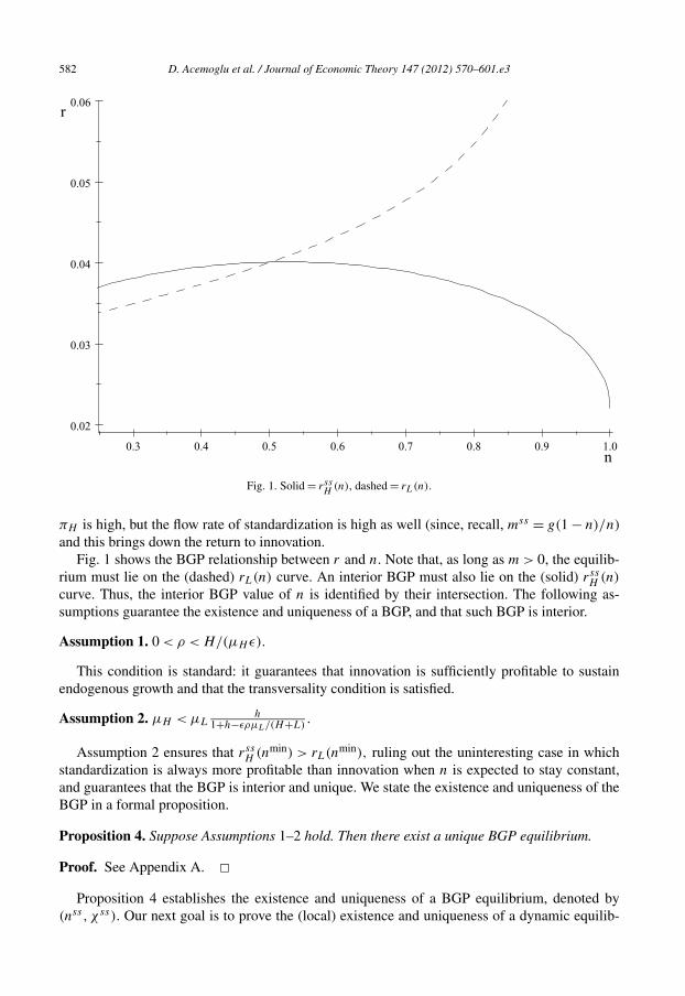
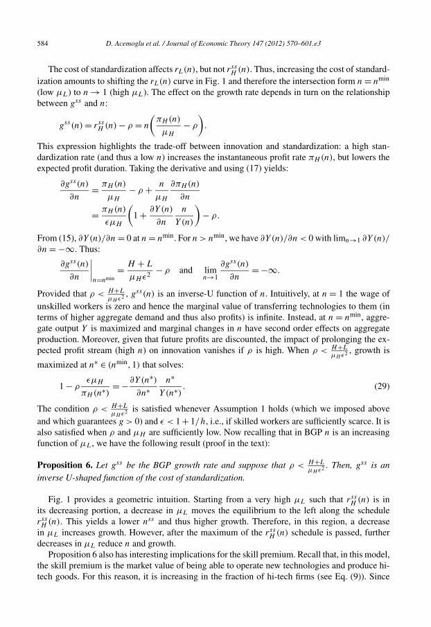
Fig. 1. Solid = rssH

(n), dashed = rL(n).

πH is high, but the flow rate of standardization is high as well (since, recall, mss = g(1 − n)/n)and this brings down the return to innovation.

Fig. 1 shows the BGP relationship between r and n. Note that, as long as m > 0, the equilib-rium must lie on the (dashed) rL(n) curve. An interior BGP must also lie on the (solid) rss

H (n)

curve. Thus, the interior BGP value of n is identified by their intersection. The following as-sumptions guarantee the existence and uniqueness of a BGP, and that such BGP is interior.

Assumption 1. 0 < ρ < H/(μH ε).

This condition is standard: it guarantees that innovation is sufficiently profitable to sustainendogenous growth and that the transversality condition is satisfied.

Assumption 2. μH < μLh

1+h−ερμL/(H+L).

Assumption 2 ensures that rssH (nmin) > rL(nmin), ruling out the uninteresting case in which

standardization is always more profitable than innovation when n is expected to stay constant,and guarantees that the BGP is interior and unique. We state the existence and uniqueness of theBGP in a formal proposition.

Proposition 4. Suppose Assumptions 1–2 hold. Then there exist a unique BGP equilibrium.

Proof. See Appendix A. �Proposition 4 establishes the existence and uniqueness of a BGP equilibrium, denoted by

(nss, χss). Our next goal is to prove the (local) existence and uniqueness of a dynamic equilib-


rium converging to this BGP. Unfortunately, the analysis of dynamics is complicated by severalfactors. First, the dynamical system (21)–(22) is highly nonlinear. Second, it may exhibit dis-continuities in the standardization rate (and thus in the interest rate) along the equilibrium path.Intuitively, at (nss, χss) there is both innovation and standardization (otherwise we could nothave n = 0). It is relatively easy to prove that, similar to models of directed change (e.g., [2,8]),there exists a dynamic equilibrium converging to the BGP featuring either only innovation (whenn < nss ) or only standardization (when n > nss ). This implies that when the economy approachesthe BGP from the left, the standardization rate and the interest rate both jump once the BGP isreached. In particular, when n < nss , there is no standardization, thus, m = 0, while in BGPwe have m > 0. Since throughout there is innovation, the value of hi-tech firms must remainconstant at VH = μH and thus there can be no jump in r + m. Consequently, there must be anexactly offsetting jump in interest rate r when the BGP is reached and the standardization rate,m, jumps.10

However, it turns out to be more difficult to prove that there exist no other dynamic equi-libria. In particular, we must rule out the existence of equilibrium trajectories (solutions to(21)–(22)) converging to (nss, χss) with both innovation and standardization when the econ-omy is away from the BGP. Numerical analysis suggests that no such trajectory exists as longas Assumptions 1 and 2 are satisfied. In particular, the system (21)–(22), under the conditionthat m = πH (n)/μH − πL(n)/μL (i.e., under the condition that there is both innovation andstandardization), is globally unstable around (nss, χss). However, we can only prove this an-alytically under additional conditions. In particular, we must impose the following parameterrestriction11:

ε − 1

ε(h + 2) + ε >

2h + 1

h(h + 1). (28)

Proposition 5. Suppose that Assumptions 1 and 2 and (28) hold. Then there exists ρ > 0 suchthat, for ρ < ρ, the interior BGP is locally saddle-path stable. In particular, if nt0 is in theneighborhood of its BGP value, nss , and nt0 > nss [resp., nt0 < nss ], then there exists a uniquepath converging to the BGP such that for some finite t > t0, we have τ ∈ [t0, t], mτ > 0, gτ = 0and nτ < 0 [resp., mτ = 0, gτ > 0 and nτ > 0], and the economy attains the BGP at t (i.e., forall τ � t , we have nτ = nss , mτ = mss , and gτ = gss ).

Proof. See Appendix A. �2.7. Growth and standardization: an inverse-U relationship

How does the cost of standardization, μL, affect the BGP growth rate, gss? Answering thisquestion is important from both a normative and a positive perspective. First, policies such asIPR protection are likely to have an impact on the profitability of standardization. Therefore,knowing the relationship between standardization and growth is a key step for policy evaluation.Second, the difficulty of standardization and hence its costs may vary across technologies andover time.

10 Note that the discontinuous behavior of the standardization rate and the interest rate does not imply a jump in theasset values, VH and/or VL. Rather, the rate of change of these asset values may jump locally.11 This restriction, which ensures that nmin = h/(1 + h) is not too small, is used in Appendix A. For example, whenε = 2, it requires nmin = h/(1 + h) > 0.28 and when ε = 3, nmin = h/(1 + h) > 0.21.


The cost of standardization affects rL(n), but not rssH (n). Thus, increasing the cost of standard-

ization amounts to shifting the rL(n) curve in Fig. 1 and therefore the intersection form n = nmin

(low μL) to n → 1 (high μL). The effect on the growth rate depends in turn on the relationshipbetween gss and n:

gss(n) = rssH (n) − ρ = n

(πH (n)

μH

− ρ

).

This expression highlights the trade-off between innovation and standardization: a high stan-dardization rate (and thus a low n) increases the instantaneous profit rate πH (n), but lowers theexpected profit duration. Taking the derivative and using (17) yields:

∂gss(n)

∂n= πH (n)

μH

− ρ + n

μH

∂πH (n)

∂n

= πH (n)

εμH

(1 + ∂Y (n)

∂n

n

Y (n)

)− ρ.

From (15), ∂Y (n)/∂n = 0 at n = nmin. For n > nmin, we have ∂Y (n)/∂n < 0 with limn→1 ∂Y (n)/

∂n = −∞. Thus:

∂gss(n)

∂n

∣∣∣∣n=nmin

= H + L

μH ε2− ρ and lim

n→1

∂gss(n)

∂n= −∞.

Provided that ρ < H+L

μH ε2 , gss(n) is an inverse-U function of n. Intuitively, at n = 1 the wage ofunskilled workers is zero and hence the marginal value of transferring technologies to them (interms of higher aggregate demand and thus also profits) is infinite. Instead, at n = nmin, aggre-gate output Y is maximized and marginal changes in n have second order effects on aggregateproduction. Moreover, given that future profits are discounted, the impact of prolonging the ex-pected profit stream (high n) on innovation vanishes if ρ is high. When ρ < H+L

μH ε2 , growth is

maximized at n∗ ∈ (nmin,1) that solves:

1 − ρεμH

πH (n∗)= −∂Y (n∗)

∂n∗n∗

Y(n∗). (29)

The condition ρ < H+L

μH ε2 is satisfied whenever Assumption 1 holds (which we imposed aboveand which guarantees g > 0) and ε < 1 + 1/h, i.e., if skilled workers are sufficiently scarce. It isalso satisfied when ρ and μH are sufficiently low. Now recalling that in BGP n is an increasingfunction of μL, we have the following result (proof in the text):

Proposition 6. Let gss be the BGP growth rate and suppose that ρ < H+L

μH ε2 . Then, gss is aninverse U-shaped function of the cost of standardization.

Fig. 1 provides a geometric intuition. Starting from a very high μL such that rssH (n) is in

its decreasing portion, a decrease in μL moves the equilibrium to the left along the schedulerssH (n). This yields a lower nss and thus higher growth. Therefore, in this region, a decrease

in μL increases growth. However, after the maximum of the rssH (n) schedule is passed, further

decreases in μL reduce n and growth.Proposition 6 also has interesting implications for the skill premium. Recall that, in this model,

the skill premium is the market value of being able to operate new technologies and produce hi-tech goods. For this reason, it is increasing in the fraction of hi-tech firms (see Eq. (9)). Since


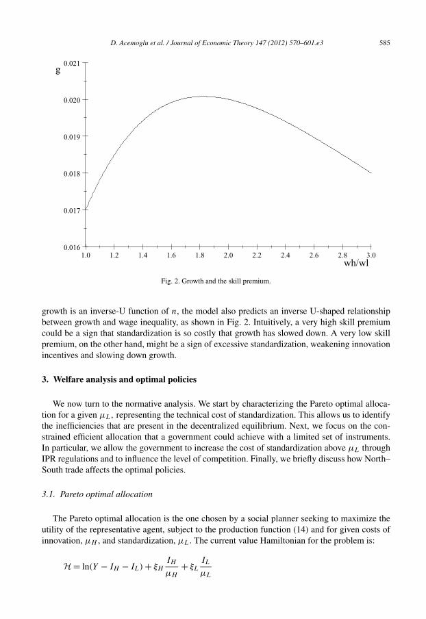
Fig. 2. Growth and the skill premium.

growth is an inverse-U function of n, the model also predicts an inverse U-shaped relationshipbetween growth and wage inequality, as shown in Fig. 2. Intuitively, a very high skill premiumcould be a sign that standardization is so costly that growth has slowed down. A very low skillpremium, on the other hand, might be a sign of excessive standardization, weakening innovationincentives and slowing down growth.

3. Welfare analysis and optimal policies

We now turn to the normative analysis. We start by characterizing the Pareto optimal alloca-tion for a given μL, representing the technical cost of standardization. This allows us to identifythe inefficiencies that are present in the decentralized equilibrium. Next, we focus on the con-strained efficient allocation that a government could achieve with a limited set of instruments.In particular, we allow the government to increase the cost of standardization above μL throughIPR regulations and to influence the level of competition. Finally, we briefly discuss how North–South trade affects the optimal policies.

3.1. Pareto optimal allocation

The Pareto optimal allocation is the one chosen by a social planner seeking to maximize theutility of the representative agent, subject to the production function (14) and for given costs ofinnovation, μH , and standardization, μL. The current value Hamiltonian for the problem is:

H = ln(Y − IH − IL) + ξH

IH + ξL

IL

μH μL


where IH and IL are investment in innovation and standardization, respectively. The controlvariables are IH and IL, while the state variables are A and AL, with co-state variables ξH

and ξL, respectively. From the first order conditions, the Pareto optimal n solves:

∂Y

∂A

1

μH

= ∂Y

∂AL

1

μL

. (30)

That is, the planner equates the marginal rate of technical substitution between hi-tech and low-tech products to their relative development costs. The Euler equation for the planner is:

C

C= ∂Y

∂A

1

μH

− ρ.

By comparing these results to those in the previous section, we can see that the decentralizedequilibrium is inefficient for two reasons.

First, there is a standard appropriability problem whereby firms only appropriate a fractionof the value of innovation/standardization so that R&D investment is too low. To isolate thisinefficiency, consider the simplest case L = 0, so that there is no standardization and Y = AH ,πH = H/ε. In this case, the social return from innovation is H while the private return is onlyr = H/ε < H . The same form of appropriability effect also applies when L > 0.

Second, there is too much standardization relative to innovation due to a business stealingexternality: the social value of innovation is permanent while the private benefit is temporary.A particularly simple case to highlight this inefficiency is when ε = 2 so that (30) simplifies to:

n

1 − n= h

(μL + μH

μH

)2

.

In the decentralized equilibrium, instead, the condition rL(n) = rssH (n) yields:

n

1 − n= h

[(r

m + r

)μL

μH

]2

.

Clearly, n is too low in the decentralized economy.To correct the first inefficiency, subsidies to innovation (and standardization) are needed. On

the other hand, the business stealing externality can be corrected by introducing a licensing policyrequiring low-tech firms to compensate the losses they impose on hi-tech firms. In particular,suppose that firms that standardize must pay a one-time licensing fee μlic

L to the original inventor.In this case, the free-entry conditions together with the Hamilton–Jacobi–Bellman equations (18)become:

VL = πL

r= μlic

L + μL, VH = πH − m(VH − μlicL )

r= μH .

Clearly, the business stealing effect is removed when μlicL = μH , that is, when low-tech firms

compensate the hi-tech produces for the entire capital loss μH . We summarize these results inthe proposition (proof in the text).12

Proposition 7. The Pareto optimal allocation can be decentralized using a subsidy to innovationand a license fee imposed on firms standardizing new products.

12 Note that there is no static distortion due to monopoly pricing. This is because in our model all firms only useinelastically supplied factors (skilled and unskilled labor). Thus, markups do not distort the allocation. In a more generalmodel, subsidies to production would also be needed to correct for the static inefficiency.


3.2. Constrained efficiency: optimal μL

Proposition 7 shows how the Pareto optimal allocation can be decentralized. However, thesubsidies to innovation require lump-sum taxes and in addition, the government would need toset up and operate a system of licensing fees. In practice, both of these might be difficult.13

Motivated by this reasoning, we now analyze a constrained efficient policy, where we limit theinstruments of the government. In particular, we assume that the government can only affect thestandardization cost through IPR regulations restricting the access to new technologies, and askwhat would the optimal policy be in this case.14 More precisely, we find the (constant) μ∗

L thatmaximizes BGP utility:

maxμL

ρW = ρ

∞∫0

[ln

(C

A

)+ ln

(A0e

gt)]

e−ρtdt = ln(χss

) + gss

ρ. (31)

The optimal policy maximizes a weighted sum of the consumption level and its growth rate. Inturn, gss(μL) = n[πH (n)/μH − ρ] evaluated at the n(μL) that solves (27) and χss = y(n) −g(μL)[μH + μL(1 − n)], evaluated at the same n. In general, problem (31) does not have aclosed-form solution. Nonetheless, we can make progress by considering two polar cases.

3.2.1. Optimal/growth maximizing policy: ρ → 0As ρ → 0, the optimal policy is to maximize gss . For this case, we have simple analytic

results. Manipulating the first order condition (29), the optimal n∗ is implicitly defined by:

(1 − n∗

n∗ h

) ε−1ε = 1 − 1

n∗

(1 − 1

ε

). (32)

Note that the LHS is decreasing in n, from infinity to zero, while the RHS is increasing in n,ranging from minus infinity to 1/ε. Thus, the solution n∗ is always interior and unique. Usingthe implicit function theorem yields:

∂n∗

∂ε

ε

n∗ = ε(1 − n∗)ε − 1

> 0 and∂n∗

∂h

h

n∗ = (1 − n∗)(1 − ε + n∗ε

)> 0 (33)

because, from (32), εn∗ − ε + 1 = ε(n∗) 1ε (1 − n∗) ε−1

ε hε−1ε > 0. That is, the optimal fraction of

hi-tech goods is increasing in the relative skill-endowment and in the elasticity of substitutionacross products.

Once we have n∗, we can use the indifference condition between innovation and standardiza-tion, VH

VL= μH

μL, to solve for the μ∗

L that implements n∗. When ρ → 0 and m = g(1 − n)/n we

13 Licensing may fail in practice because of incompleteness of contracts or because of asymmetric information(e.g., [17]). See also [23] on the difficulties of using market signals to determine the value of existing innovations.14 We do not consider patent policies explicitly because we view them as only one source of competitive advantage forincumbents. In particular, patents are generally thought to be less important than lead time and learning-curve advantagein preventing duplication. Their utility might often be limited by the fact that they require disclosure of information,which would otherwise remain trade secret, and the application process is often lengthy and cannot prevent competitorsfrom “inventing around” patents. Overall, Levin et al. [47] found that patents increase imitation costs by 7–15%. Thissupports both our approach of modeling IPR protection as an additional cost of standardization and the notion that patentsare only one of the many factors making standardization costly.


obtain:

πH

πL

= μH

μL

1

n→

(1 − n

nh

) ε−1ε = μH

μL

1

n. (34)

The equilibrium fraction of hi-tech goods, n, depends on relative profits (πH /πL), relative R&Dcosts (μH /μL), and the standardization risk faced by hi-tech firms (captured by the factor 1/n).Note that a decline in the relative skill supply, h, leads to a more than proportional fall in n

because πH /πL falls and m rises. Substituting ( 1−n∗n∗ h)

ε−1ε from (32) we can find the optimal

standardization cost as:

μ∗L = μH

(n∗ − 1 + 1

ε

)−1

= μH ε

1 − ε + n∗ε. (35)

This expression has the advantage that it only depends on h through n∗ and can be used tostudy the determinants of the optimal policy. Differentiating (35) and using (33), we obtain thefollowing proposition (proof in the text).

Proposition 8. Consider the case ρ → 0. BGP welfare and growth are maximized when the costof standardization μL satisfies (35) and n∗ is the solution to (32). The following comparativestatic results hold:

∂μ∗L

∂μH

μH

μ∗L

= 1,

∂μ∗L

∂h

h

μ∗L

= −εn∗(1 − n∗) < 0,

∂μ∗L

∂ε

ε

μ∗L

= n∗ε − 1

ε − 1> 0.

The results summarized in this proposition are intuitive. Changes in the cost of innovationshould be followed by equal changes in the cost of standardization, so as to keep the optimaln constant. A decline in the relative supply of skilled workers makes technology diffusion rela-tively more important. However, the incentive to standardize increases so much (both because ofthe change in instantaneous profits and because the equilibrium m increases too) that the optimalpolicy is to make standardization more costly. Thus, somewhat surprisingly, a higher abundanceof unskilled worker calls for stronger IPR protection. Finally, given that ε � 2, a lower elastic-ity of substitution makes the diffusion of technologies to low-skill workers more important foraggregate productivity and reduces the optimal IPR, μ∗

L.15

3.2.2. Optimal policy: high ρ

To understand how the optimal policy changes with the discount rate, we consider the otherpolar case. In particular, assume that ρ → H+L

μH ε. As we will see, this is the highest ρ compatible

with positive growth. In this case, Section 2.7 shows that g is maximized at the corner nmin =h/(h + 1). Moreover, for n → nmin we have πH = L+H

εand g = H+L

μH ε− ρ → 0 (since ρ →

H+LμH ε

). Next, the result that g must be close to zero yields χss = y, which is also maximized

15 To see this, recall that εn∗ − ε + 1 > 0. Then, ε � 2 implies (εn∗ − 1)/(ε − 1) > 0.


at nmin. Thus, with high discounting the optimal policy is the same as the one that maximizesstatic output (and consumption) only. Reaching this point requires setting μ∗

L = μH . Note that,in this extreme scenario, the optimal policy becomes independent of h and other parameters.Comparing the policy μ∗

L = μH to (35) shows, not surprisingly, that high discounting implies alower optimal protection of IPR.

3.3. Other competition policies

In practice, several other competition policies, besides licensing fees and intellectual propertyrights, are used in order to affect the profitability of standardization. We now briefly discussthe implications of such policies. Suppose that the government can directly affect markups inthe hi-tech and the low-tech sectors. In particular, it can set εH � ε and εL � ε in the pricingequations (5).

When markups vary across firms, profits (16) become:

πL = y1/ε

εL

(L

1 − n

) ε−1ε

and πH = y1/ε

εH

(H

n

) ε−1ε

. (36)

From rL(n) = πL/μL and the above expressions, it is immediate to see that the BGP n onlydepends on the product μLεL. This result highlights that competition policy (εL) and IPR pro-tection (μL) are substitutes. Intuitively, with lower mark-ups (high εL) for low-tech firms, thereis less entry in the L-sector. Yet, the government can offset this effect by reducing μL, so that itbecomes easier to standardize. On the contrary, gss(n) does not depend on εL, so that n∗ is asbefore. Given that intervening on μL or εL is equally effective to implement a desired n∗, theoptimal mix depends on the relative costs of the two policies.

Now when we also have ρ → 0, Eq. (35) becomes:

μL = εH

εL

· μH ε

1 − ε + n∗ε. (37)

Then, under the assumptions that εL can be changed at no cost, it is easy to see that the optimalpolicy is:

εH = ε,

μ∗L = μmin

L ,

εL = εH

μminL

· μH ε

1 − ε + n∗ε,

where μminL � 0 is the minimum “technical” cost of standardization (i.e., with no IPR protection).

Intuitively, full monopoly among hi-tech firms ensures high innovation; μ∗L = μLmin minimizes

the resources spent on standardization; high competition among low-tech firms yields the opti-mal n∗. If the desired level of competition εL cannot be achieved, then μ∗

L should be adjustedupward accordingly.16

16 Another way to highlight the same result is that policy does not affect markups, but rather patent duration in the low-tech sector. In the model considered so far, patent length is infinite in the low-tech sector. Suppose, however, that patentduration is finite and, once the patent expires, the good is produced by unskilled workers under competitive conditions.Here, the key trade-off is between the cost of standardization and the duration of the subsequent monopoly position inthe low-tech sector. The gist of the argument is that the best combination is, in a sense, low IPR everywhere (low μL andshort patents). However, it has to be carefully tailored, since the cost-relative-to-duration must be pinned down so as toget the right n.


3.4. North–South trade and IPR policy

We now ask how trade opening in countries with a large supply of unskilled workers affects theoptimal IPR policy. This question is interesting because there is an unsettled debate on whethertrade liberalization in less developed countries should be accompanied by tighter IPR protection,as implied by the TRIPS Agreement, or by less strict IPR policies, which serve to encourage tech-nology diffusion to less advanced economies. We can investigate this question using our model.

Consider an integrated world economy (the North), described by the model in Section 2.For simplicity, let us also assume that there is a single large developing country endowed withunskilled workers only (the South). Without trade, we assume that Northern technologies arecopied at no cost by competitive firms in the South. However, this form of technology transferis imperfect: when a low-tech good is introduced in the South, labor productivity there is only afraction ϕ ∈ (0,1]. There is no innovation in the South.

Now imagine that the South opens its economy to trade. We assume that economic integrationallows Northern firms to produce in the South. In the new integrated equilibrium factor prices areequalized (or else firms would relocate to the country where labor is cheaper) and Southern firmsare replaced by their Northern counterpart. This result stems from the fact that Northern firmsare more productive and can capture the entire market by charging a price equal to or lower thanthe marginal cost of the Southern imitators, pL � wL/ϕ. However, if ϕ > (1 − 1/ε), Northernfirms must compress their markup to keep Southern imitators out.

In sum, the effect of trade opening in the South is isomorphic to an increase in the worldendowment of L and possibly a reduction in the markup and profit margins of low-tech firms(higher εL). What are the implications for the BGP growth rate and the optimal IPR policy? Thechange in L and εL have opposite effects on πL (see Eq. (36)) and hence on the return fromstandardization, so the rL(n) curve in Fig. 1 may either shift up or down. The rss

H (n) curve,instead, always shifts up because the greater supply of low-tech goods increases the price andthus the profitability of hi-tech products. As a result, in the new BGP, nss and gss may be higheror lower. Despite this ambiguity, it is easy to see that trade opening is necessarily growth (andwelfare) enhancing if IPR policy, μL, is correctly adjusted. This follows immediately from theupward shift of the rss

H (n) curve, implying that the maximum attainable r must be higher.The crucial question, then, is how μL should be changed. As already seen, a lower h increases

the optimal level of IPR protection, μ∗L. On the other hand, higher competition among low-

tech firms, εL, calls for a reduction in μL, to compensate for the fall in profit margins (seeEq. (37)). The net effect depends on which force dominates. If the liberalizing country is largeand inefficient (low ϕ), the competitive pressure posed by imitators on low-tech firms is weak,while the threat to hi-tech firms, due to the increased incentives to standardize, is high. In thiscase, integration should be followed by a tightening of IPR policies.17

4. Multiple equilibria and poverty traps

We have so far imposed a specific tie-breaking rule, assuming that when wH = wL the incum-bent will fight the entrance (not existing at stage (ii) of the entry-exit game). This assumption

17 These are the policies that a world planner would choose starting from the optimum. Yet, governments of individualcountries face different incentives, because an increase in μL leads to a higher skill premium and redistributes incometoward skill-abundant countries. This conflict of interests between the North and the South is studied, among others, byGrossman and Lai [36].


implies that standardization only takes place when it is strictly profitable and therefore, n nec-essarily stays in the range (nmin,1), since at n = nmin we would have wH = wL and givenincumbent behavior, standardization would lead to negative profits. Under this tie-breaking rule,Proposition 4 established the uniqueness of a BGP equilibrium. In this section, we show thatunder the alternative tie-breaking rule, whereby at wH = wL incumbents facing the entry ofa low-tech competitor exit, the model may generate multiple equilibria and potential povertytraps.18

Throughout this section, we assume a different tie-breaking rule, by which competition be-tween hi-tech incumbents and entrants at wH = wL is resolved by incumbents exiting at stage(ii) of the entry-exist game. Clearly, even under this alternative tie-breaking rule, equilibriummust involve wH � wL for any n ∈ [0,1] since skilled worker can always take unskilled jobs.But in contrast to Proposition 1 now standardization may continue even at n � nmin.

As a first step in the analysis of this case, we characterize the static equilibrium for low levelsof n. Recall that wH = wL at n = nmin. For n � nmin, the skill premium is constant at wH = wL

and some high skill workers are employed in low-tech firms. In this case, the allocation of laborbetween the two type of firms, h, is determined endogenously by Eq. (9) after setting wH = wL.This yields h = n/(1 − n) and a profit rate of πH = πL = L+H

ε. In other words, for sufficiently

low n, it is as if workers were perfect substitutes, prices are equalized pH = pL, and so areprofits.

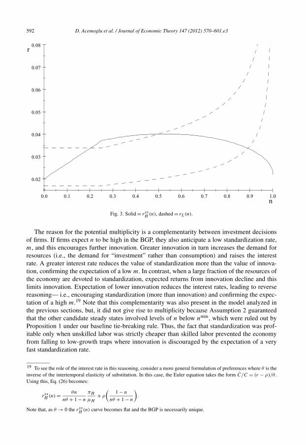
To find the steady states, we draw the rL(n) and rssH (n) schedules over the entire domain

n ∈ [0,1]. Fig. 3 shows the determination of nss for two possible rL(n) schedules, correspondingto different values of μL. Compared to Fig. 1, the first part of both schedules is a straight line, asthere the skill premium is constant and equal to one. The interior BGPs are again the intersectionsbetween the rss

H (n) (solid line) and rL(n) (dashed line) schedules.In addition to balanced growth equilibria, now there might exist “corner steady-states” such

that n = g = m = 0 and r = ρ. A corner steady state can arise in two different circumstances:(i) at n = 0, there is no incentive to innovate nor to standardize, i.e., ρ > πL

μL= H+L

μLεand ρ >

πH

μH= H+L

μH ε; (ii) at n = 0, firms have an incentive to standardize, i.e., ρ < H+L

μLε, but there are no

goods to standardize, since n = 0. Moreover, innovation is discouraged by the expectation thatnew hi-tech goods would trigger a high standardization rate. Formally, innovating firms expectthat m > H+L

μH ε−ρ whenever n > 0. This conjecture does not violate the resource constraint since

the absolute investment in standardization would be infinitesimal when n = 0 even though thestandardization rate is very high. The uninteresting case in which rL(n) lays above rss

H (n) for alln is still ruled out by Assumption 2.

As shown in Fig. 3, depending on the standardization cost, there are two regimes:

High μL: For μL > (H +L)/(ρε) (lower rL(n) schedule in Fig. 3), there is a unique steady state(BGP) corresponding to the unique crossing point of the rL(n) and rss

H (n) schedules.Low μL: For μL < (H + L)/(ρε) (upper rL(n) schedule) there are two interior and a corner

steady state. The two interior steady states can be seen in Fig. 3. In this case, a cornersteady state also exists, since rss

H (0) = ρ < rL(0) = (H + L)/(μLε). Hence, standard-ization is profitable at n = 0.

18 Multiple equilibria can also arise if we relax Assumption 2, while maintaining the same tie-breaking rule as in theanalysis so far. However, this happens for a smaller set of parameter values. We therefore focus on relaxing the tie-breaking rule while maintaining Assumption 2.


Fig. 3. Solid = rssH

(n), dashed = rL(n).

The reason for the potential multiplicity is a complementarity between investment decisionsof firms. If firms expect n to be high in the BGP, they also anticipate a low standardization rate,m, and this encourages further innovation. Greater innovation in turn increases the demand forresources (i.e., the demand for “investment” rather than consumption) and raises the interestrate. A greater interest rate reduces the value of standardization more than the value of innova-tion, confirming the expectation of a low m. In contrast, when a large fraction of the resources ofthe economy are devoted to standardization, expected returns from innovation decline and thislimits innovation. Expectation of lower innovation reduces the interest rates, leading to reversereasoning— i.e., encouraging standardization (more than innovation) and confirming the expec-tation of a high m.19 Note that this complementarity was also present in the model analyzed inthe previous sections, but, it did not give rise to multiplicity because Assumption 2 guaranteedthat the other candidate steady states involved levels of n below nmin, which were ruled out byProposition 1 under our baseline tie-breaking rule. Thus, the fact that standardization was prof-itable only when unskilled labor was strictly cheaper than skilled labor prevented the economyfrom falling to low-growth traps where innovation is discouraged by the expectation of a veryfast standardization rate.

19 To see the role of the interest rate in this reasoning, consider a more general formulation of preferences where θ is theinverse of the intertemporal elasticity of substitution. In this case, the Euler equation takes the form C/C = (r − ρ)/θ .Using this, Eq. (26) becomes:

rssH (n) = θn

nθ + 1 − n

πH

μH+ ρ

(1 − n

nθ + 1 − n

).

Note that, as θ → 0 the rss (n) curve becomes flat and the BGP is necessarily unique.
H


We summarize the characterization of the set of steady-state equilibria in the following propo-sition (proof in the text).

Proposition 9. Suppose that Assumptions 1 and 2 hold and adopt the tie-breaking rule that whenwH = wL, incumbents exit in state (ii) of the sequential entry-exit game. Then:

1. If μL > (H + L)/(ρε), there exists a unique BGP which is interior.2. If μL < (H + L)/(ρε), there exist two interior BGP equilibria and a corner steady state.

It is also noteworthy that the non-monotonic relationship between the gss and μL and thepolicy analysis derived in the previous sections now apply to the higher interior BGP. The mainnovelty, however, is that too low a cost of standardization may lead to multiple steady states,one of them in fact corresponding to stagnation, and the exact equilibrium path is determined byself-fulfilling expectations.

5. Concluding remarks

New technologies often diffuse as a result of costly adoption and standardization decisions.Such standardization also creates cheaper ways of producing new products, for example, substi-tuting cheaper unskilled labor for the more expensive skilled labor necessary for the production ofnew complex products. This process endogenously generates competition to original innovators.In this paper, we studied the implications of this costly process of standardization, emphasizingboth its role as an engine of growth and its potential negative effects on innovation (because ofthe “business stealing” effect that it creates).

Our analysis has delivered a number of new results. First, the tension between innovation andstandardization generates an inverse U-shaped relationship between competition and growth.Second, while technology diffusion is potentially beneficial, it can also have destabilizing ef-fects. Standardization can open the door to multiple equilibria (multiple growth paths). Finally,we characterized the optimal competition and IPR policy and how it depends on endowmentsand other parameters, such as the elasticity of substitution between products. We found that in-novation rents should be protected more when skilled workers are perceived as scarcer, that is,when they are in short supply and when the elasticity of substitutions between goods is high. Wealso showed that these results provide new reasons for linking North–South trade to intellectualproperty rights protection.

It is also worth noting that a key feature of our analysis is the potential competition betweenstandardized products and the original hi-tech products. We believe that this is a good approx-imation to a large number of cases in which standardization takes place by different firms (andoften in the form of slightly different products). Nevertheless, the alternative, in which standard-ization is carried out by the original innovator, is another relevant benchmark. In our follow-upwork [7], we study a model of offshoring, where offshoring can be viewed as a costly process ofstandardization carried out by the original innovator to make goods producible in less developedcountries with cheaper labor.

Our model yields a number of novel predictions that can be investigated empirically. In par-ticular, it suggests that competition and IPR policy should have an impact on skill premia.Furthermore, data on product and process innovation might be used to test the existence of atrade-off between innovation and standardization at the industry level. These seem interestingdirections for future work.


Appendix A

A.1. Proof of Lemma 1

Recall πH = pH HεH AH

= pH HεH nA

. From (11) it is immediate to see that ∂πH

∂n< 0 if pH � pL, which

is true in equilibrium. To establish the properties of πL, note that:

∂(ε − 1) lnπL

∂n=

1ε( n

1−n)

ε+1ε ( 1

n2 )hε−1ε

1 + ( n1−n

)1ε h

ε−1ε

+ ε − 2

1 − n> 0 if ε > 2 −

1ε

1nh

ε−1ε

( 1−nn

)1ε + h

ε−1ε

.

For ε � 2, lim n→1∂πL

∂n= ∞. Convexity of πL follows immediately because the function ∂πL

∂nhas

no critical point.

A.2. Notes on figures

The benchmark economy used to draw all figures has the following parameter values:

ρ = 0.02; ε = 2; μH = 22.7, μL = 59.1; H = 1; L = 3

implying in steady state:

g = 0.02; r = 0.02; m = 0.02; n = 0.5; wH

wL

= 1.5.

A.3. Proof of Proposition 4

A BGP must be a rest point of the dynamical system (21)–(22). We first note that there cannotbe a rest point at the boundaries n = nmin and n = 1 in view of Proposition 1. Thus any BGP mustbe interior as defined in Proposition 3, or equivalently, it must be a zero of the dynamical system(21)–(22). We denote such a zero by (nss, χss), where nss satisfies rL(nss) = rss

H (nss) (see againProposition 3). We prove the existence of a unique interior BGP by showing that there is a uniquevalue nss ∈ (nmin,1) such that rL(nss) = rss

H (nss), that there is a unique corresponding value ofχss and that at (nss, χss) the transversality condition is satisfied.

We prove the first step by establishing that rssH (nss) is a continuous inverse U-shaped function

whereas rL(nss) is a continuous, increasing and convex function. Moreover rssH (nmin) > rL(nmin)

(from Assumption 2) and limn→1(rL(nss) − rssH (nss)) = ∞. Then, the intermediate value the-

orem establishes the existence of such a BGP, while the shape of the two functions implies

uniqueness. Let φ(x) ≡ [x +x( 1x

−1)1ε h

1−εε ] 1

ε−1 where ε � 2 and h � 0. Standard algebra estab-lishes that φ(x) is a continuous inverse U-shaped concave function, such that limx→0 φ′(x) = ∞and limx→1− φ′(x) = −∞. Thus, φ(x) has a unique interior maximum in the unit interval.Next, note that rss

H (nss) = φ(nss) · H/(μH ε) + (1 − nss)ρ. Since rssH (nss) is a linear trans-

formation of φ(nss), it is also a continuous inverse U-shaped concave function, with a uniqueinterior maximum in the unit interval. Consider now rL(nss). Since rL(nss) = πL(nss)/μL,Lemma 1 establishes that rL(nss) is increasing and convex, with limnss→1 rL(nss) = ∞ (thus,limnss→1[rL(nss) − rss

H (nss)] = ∞).Next, straightforward algebra immediately implies that, conditional on n = nss and m =

m(nss), there exists a unique value χ = χss that yields a zero of the dynamical system (21)–(22). Finally, since in BGP r = ρ + g > g (from (1) and Assumptions 1–2), the transversalitycondition is satisfied in the unique candidate BGP.


A.4. Proof of Proposition 5

Recall that dynamic equilibria are given by solutions to dynamical system (21)–(22) withboundary conditions given by the initial condition n = n0 and the transversality condition. Bythe same argument as in the proof of Proposition 4, there cannot be any dynamic equilibriumpath where n → nmin and n → 1. Any dynamic equilibrium must thus either converge to theunique (interior) BGP (nss, χss) or involves cycles. We will show in this proof that startingfrom any initial condition n = n0 in the neighborhood of nss (the BGP), there exists a uniquepath converging to (nss, χss) and that there cannot be cycles, thus establishing local saddle-pathstability of the dynamic equilibrium.

Because there are two sources of technical change (innovation and standardization), we firstdistinguish between three possible types of potential dynamic equilibria (which may converge tothe BGP, (nss, χss)).

Case 1. VH = μH and VL < μL (⇒ m = 0 and g = (y(n) − χ)/μH ). In this case, from Propo-sition 3 the dynamics are governed by the following system of ordinary differential equations:

χ

χ= πH (n)

μH

− ρ − y(n) − χ

μH

, n = (1 − n)y(n) − χ

μH

. (38)

Case 2. VH < μH and VL = μL (⇒ m = (y(n) − χ)/(nμL) and g = 0). In this case, againfrom Proposition 3 the dynamics are governed by the following system of ordinary differentialequations:

χ

χ= πL(n)

μL

− ρ, n = −(

y(n) − χ

μL

). (39)

Case 3. VH = μH and VL = μL (⇒ m = πH (n)/μH −πL(n)/μL and g = (y(n)−μLmn−χ)/

μH ). In this case, the dynamics are governed by the following system of ordinary differentialequations:

χ

χ= πL(n)

μL

− ρ − y(n) − μLmn − χ

μH

,

n = (1 − n)y(n) − χ

μH

− mn

(1 + (1 − n)

μL

μH

). (40)

In all three cases, the differential equations are defined over the region χ ∈ [0, y(n)], n ∈[nmin,1]. Recall that in the BGP m > 0 and g > 0. This implies that VH = μH and VL = μL.

Therefore, (nss, χss) is a zero of the dynamical system (40), but it is not a zero either of (38) orof (39). Nevertheless, we will show that Case 3 cannot describe dynamic equilibrium behaviorat any point with (n,χ) �= (nss, χss). Instead, the equilibrium dynamics will be given by eitherCase 1 or Case 2 (depending on whether n is above or below nss ) and will be unique. Thenunder the equilibrium dynamics, the economy will converge in finite time to (nss, χss), and thena jump in m and r will create a switch to Case 3 at that point. Since (nss, χss) is a zero of (40),the economy will have reached the BGP and will stay at (nss, χss) thereafter.

We prove the result by first establishing several lemmas. First, Lemma 2 establishes that, ifn < nss, there exists a unique trajectory converging to (nss, χss) (it is immediate that, if n < nss ,there exists no trajectory converging to (nss, χss) following the dynamics (39), since these would


imply n � 0). Second, Lemma 3 establishes that, if n > nss, there exists a unique trajectoryconverging to (nss, χss) following the dynamics (39) (it is immediate that, if n > nss , there existsno trajectory converging to (nss, χss) following the dynamics given by (38), since these implyn � 0). Third, Lemma 4 provides a complete characterization of equilibrium dynamics when thetransition involves either only innovation or only standardization, followed by a jump in eitherthe innovation or the standardization rate as the economy reaches (nss, χss), but continuouschanges in asset values. Fourth, Lemma 5 establishes that (under the sufficient conditions ofthe proposition) there exists no trajectory converging to (nss, χss) following the dynamics (40).Finally, Lemma 6 rules out transitional dynamics in the neighborhood of the BGP in which thereis a jump from Case 3 to either Case 1 or Case 2 or between Cases 1 and 2. These lemmastogether establish local saddle-path stability.

Lemma 2. Suppose n0 < nss. Then, there exists a unique trajectory attaining (nss, χss) in finitetime following the dynamics of Case 1, (38). This trajectory features monotonic convergence inn (n > 0).

Proof. Consider the system of differential equations (38). This system has no zero over the feasi-ble region [nmin,1]×[0, y(n)]. In particular, in the interior of the region [nmin,1]×[0, y(n)], andhence at (nss, χss), n > 0 and χ � 0 ⇔ χ � χ(n), where χ(n) = μH ρ + y(n) − πH (n) < y(n).

The last inequality follows from Assumption 1. Although whether χ (nss) � χ(nss) is in generalambiguous, there is a unique trajectory (and a unique initial level of the control variable, χ0) con-verging in finite time to (nss, χss). In particular, since (nss, χss) is not a zero of the system (38),the determination of the converging trajectory can be expressed as an initial value problem with(nss

T ,χssT ) being the boundary (terminal) condition. From the standard result of existence and

uniqueness of solutions for systems of ordinary differential equations, this initial value problemhas a unique solution. Fixing the initial condition n0 yields a unique solution for T (the length ofthe transition) and χ0. The monotonicity of the dynamics of n ensures that this solution is unique,i.e., there does not exist two solutions (n0, T ,χ0) and (n0, T

′, χ ′0) with T �= T ′ and χ0 �= χ ′

0. Thisargument also proves that convergence is attained in finite time. �Lemma 3. Suppose n0 > nss. Then, there exists a unique trajectory attaining (nss, χss) in finitetime following the dynamics of Case 2, (39). This trajectory features monotonic convergence(n < 0 and χ > 0).

Proof. The proof is similar to that of Lemma 2. The dynamical system again has no zero over thefeasible region [nmin,1] × [0, y(n)]. In particular, for n0 � nss , n > 0 and χ > 0. The latter fol-lows from the observation that χ � 0 ⇔ πL(n)/μL � ρ, where π ′

L(n) < 0 and πL(nss)/μL > ρ,

implying that πL(n)/μL > ρ for all n � nss . Standard properties of systems of ordinary differ-ential equations establish that there is a unique trajectory converging in finite time to (nss, χss)

and this trajectory features monotonic dynamics. �The previous two lemmas together imply our key characterization result.

Lemma 4. There exists equilibrium dynamics with the following characteristics.If n0 < nss, the economy converges in finite time to (nss, χss) following the system of

differential equations (38), with monotonic convergence in n. Throughout this convergence,VH = μH , VL < μL, m = 0 and g = (y(n) − χ)/μH . When the economy reaches (nss, χss),

there is a discrete increase in standardization offset by a fall in the interest rate such thatr(nss) = r ′(nss) + m(nss). Thereafter, VH = μH and VL = μL.


If n0 > nss the economy converges in finite time to (nss, χss) following the system of differ-ential equations (39), with monotonic convergence in n and χ. Throughout this convergence,VH < μH , VL = μL, m = (y(n) − χ)/(nμL) > 0 and g = 0. When the economy reaches(nss, χss), there is a discrete fall in standardization offset by an increase in innovation suchthat y(nss) − χ remains constant. Thereafter, VH = μH and VL = μL.

Proof. The proof follows from Lemmas 2 and 3 combined with the following observations. Sup-pose we start with n0 < nss , then the dynamic equilibrium is given by the system of differentialequations (38), so from Lemma 2 until T , we have m = 0. At T , we reach (nss, χss) and m

jumps from zero to its steady state, mss . This is offset by an equal jump down in r implyingthat VH does not change (i.e., it remains at VH = μH ). Moreover, at T , VL attains its steadystate (BGP) value, VL = μL. Note that there is no discontinuity in the asset value VL, since thechange in r and m are perfectly anticipated, causing a continuous change in the value VL beforethe actual change occurs to reach VL = μL exactly at T (the continuity of VL ensures that thereis no arbitrage opportunity in buying and selling shares of L-sector firms). Thus at this point, thedynamics switch to those given by the system of differential equations (40) with both innovationand standardization. Since (nss, χss) is a zero of (40), the economy stays at (nss, χss) thereafter.The fact that this path satisfies the transversality condition follows by the same argument as inthe proof of Proposition 4.

Next, suppose that we start with n0 > nss . Then the dynamic equilibrium is given by thesystem of differential equations (39) and from Lemma 3, until T , g = 0. At T , investment instandardization and mT fall discretely (the latter declining to mss ), and investment in innovationand g jumps up (the latter increasing to gss ). There is no change in overall investment and thusneither r , nor consumption nor VL change at T . As m jumps down, VH attains its stead statevalue, VH = μH exactly at T (note that the path of VH is continuous at T , as the change inm is perfectly anticipated by investors). As a result, again at T , the dynamics switch to thosegiven by the system of differential equations (40) with both innovation and standardization. Since(nss, χss) is a zero of (40), the economy stays at (nss, χss) thereafter. The fact that this pathsatisfies the transversality condition again follows by the same argument. �

We next show that transitional dynamics converging to (nss, χss) cannot feature bothVH = μH and VL = μL since the system (40) is unstable in the neighborhood of (nss, χss).

Lemma 5. Suppose n0 �= nss. Then, under the (sufficient) conditions of the proposition, thereexists no trajectory converging to (nss, χss) following the dynamical system (40).

Proof. The proof of this lemma, which is long, is presented in Appendix B, which is availableonline. �

Lemmas 2–5 establish that in the neighborhood of (nss, χss), we must have either VH < μH

or VL < μL, implying that there is either only innovation or only standardization. However, theresults established so far do not rule out “switches” between different regimes while nt �= nss ,and thus cycles. Moreover, with such switches, the equilibrium might also be indeterminate,with multiple paths starting from some initial n0 converging to the BGP. Lemma 6 rules outall of these possibilities by showing that in the neighborhood of the BGP, there cannot be aswitch from the dynamics given by any one of (38), (39) and (40) to one of the other two. (Fornotational convenience, in this lemma, we write VH,t = μH to mean that VH,t ′ = μH for t ′ in aneighborhood of t .)


Lemma 6. Consider an equilibrium trajectory in the neighborhood of the BGP, (nss, χss). Then,there cannot be a switch from any one of (38), (39) and (40) to one of the other two, i.e., if at t0 inthe neighborhood of (nss, χss), we have VH,t0 = μH and VL,t0 = μL, then an equilibrium cannotinvolve VH,t < μH and/or VL,t < μL for t > t0; if we have VH,t0 = μH and VL,t0 < μL, then anequilibrium cannot involve VH,t < μH and/or VL,t = μL for t > t0; and if we have VH,t0 < μH

and VL,t0 = μL, then an equilibrium cannot involve VH,t = μH and/or VL,t < μL for t > t0.

Proof. We will prove that if in the neighborhood of (nss, χss), we have VH,t0 = μH andVL,t0 = μL, then an equilibrium cannot involve VH,t = μH and VL,t < μL for t > t0. The othercases are analogous.

Suppose to obtain a contradiction that this is the case and denote the last instance whereVL = μL by T (i.e., VL,T +ε < μL for ε > 0). We need to distinguish two cases. First, VL,t ′ < μL

for all t ′ > t , and second, there exists T ′ > t , such that we again have VL,T ′ = μL.

Case 1. The fact that VL,t ′ < μL for all t ′ > t contradicts the hypothesis that the equilibriumpath will converge to the BGP.

Case 2. We write VL,T as follows:

VL,T =∞∫

T

exp

(−

τ∫T

r(nν) dν

)πL(nτ ) dτ

=T ′∫

T

exp

(−

τ∫T

r(nν) dν

)πL(nτ ) dτ + exp

(−

T ′∫T

r(nτ ) dτ

)μL,

where the equality exploits the fact that by hypothesis VL,T ′ = μL. Moreover, we also have,again by hypothesis, that VL,T = μL, which implies

T ′∫T

exp

(−

τ∫T

r(nν) dν

)πL(nτ ) dτ =

(1 − exp

(−

T ′∫T

r(nτ ) dτ

))μL. (41)

Suppose next that nT > nss . By the instability result in Lemma 5, this implies nT > 0 and thusnτ > nss for all τ ∈ [T ,T ′]. But then from Lemma 1, πL(nτ ) > πL(nss) for all τ ∈ [T ,T ′].Moreover, since VH,τ = μH and VL,τ < μL, we also have that for all τ ∈ [T ,T ′],

r(nτ ) = πH (nτ )

μH

>πL(nτ )

μL

>πL(nss)

μL

= r(nss

),

where the second inequality again follows from Lemma 1 in view of the fact that nτ > nss for allτ ∈ [T ,T ′]. But then,

T ′∫T

exp

(−

τ∫T

r(nν) dν

)πL(nτ ) dτ <

( T ′∫T

exp

(−

τ∫T

r(nν) dν

)dτ

)πL(nss)

<

(1 − exp

(−

T ′∫r(nτ ) dτ

))μL,

T


where the second inequality follows from the fact that r(nτ ) < r(nss) for all τ ∈ [T ,T ′]. Thisinequality contradicts (41).

Suppose instead that nT < nss . By the instability result in Lemma 5, nT < 0 and thus nτ < nss

for all τ ∈ [T ,T ′]. Moreover, by the same reasoning for all τ ∈ [T ,T ′], πH (nτ ) > πH (nss) andsince VL,τ < μL, m(nτ ) = 0. Therefore,

VH,T =∞∫

T

exp

(−

τ∫T

(r(nν) + m(nν)

)dν

)πH (nτ ) dτ

=T ′∫

T

exp

(−

s∫T

r(nν) dν

)πH (nτ ) dτ + exp

(−

T ′∫T

r(nτ ) dτ

)μH . (42)

But since for all τ ∈ [T ,T ′]

r(nτ ) = πH (nτ )

μH

>πH (nss)

μH

the first term in (42) is strictly greater than (1 − exp(− ∫ T

tr(nτ ) dτ))μH and thus contradicts

VH,T = μH . �Lemmas 2–6 establish the results of the proposition. In particular, Lemmas 5 and 6 imply that

starting at nt �= nss in the neighborhood of the BGP we must have VH < μH or VL < μL. IfVH = μH and VL = μL, either we diverge from the BGP in view of 5, or we have to switch toa regime where VH < μH or VL < μL, which is ruled out by Lemma 6. If we have VH < μH

or VL < μL in the neighborhood of the BGP, then Lemmas 2–4 imply that there exists a uniquepath converging to the BGP. This completes the proof of the proposition. �References

[1] Daron Acemoglu, Why do new technologies complement skills? Directed technical change and wage inequality,Quart. J. Econ. 113 (1998) 1055–1090.

[2] Daron Acemoglu, Directed technical change, Rev. Econ. Stud. 69 (2002) 781–809.[3] Daron Acemoglu, Patterns of skill premia, Rev. Econ. Stud. 70 (2003) 199–230.[4] Daron Acemoglu, Modeling inefficient economic institutions, in: Advances in Economic Theory, Proceedings of

2005 World Congress, 2005.[5] Daron Acemoglu, Introduction to Modern Economic Growth, Princeton University Press, 2009.[6] Daron Acemoglu, Philippe Aghion, Fabrizio Zilibotti, Distance to frontier, selection and economic growth, J. Eur.

Econ. Assoc. 4 (2006) 37–74.[7] Daron Acemoglu, Gino Gancia, Fabrizio Zilibotti, Offshoring, innovation and wages, Mimeo, 2010.[8] Daron Acemoglu, Fabrizio Zilibotti, Productivity differences, Quart. J. Econ. 116 (2001) 563–606.[9] Philippe Aghion, Nick Bloom, Richard Blundell, Rachel Griffith, Peter Howitt, Competition and innovation: an

inverted-U relationship, Quart. J. Econ. 120 (2) (2005) 701–728.[10] Philippe Aghion, Christopher Harris, Peter Howitt, John Vickers, Competition, imitation, and growth with step-by-

step innovation, Rev. Econ. Stud. 68 (2001) 467–492.[11] Philippe Aghion, Peter Howitt, A model of growth through creative destruction, Econometrica 60 (2) (1992) 323–

351.[12] Philippe Aghion, Peter Howitt, Gianluca Violante, General purpose technology and wage inequality, J. Econ.

Growth 7 (2002) 315–345.[13] Pol Antras, Incomplete contracts and the product cycle, Amer. Econ. Rev. 95 (2005) 1054–1073.[14] Anthony Atkinson, Joseph Stiglitz, A new view of technological change, Econ. J. (1969) 573–578.


[15] David Autor, Frank Levy, Richard Murnane, The skill content of recent technological change: an empirical explo-ration, Quart. J. Econ. 118 (2003) 1279–1334.

[16] Susanto Basu, David Weil, Appropriate technology and growth, Quart. J. Econ. 113 (1998) 1025–1054.[17] James Bessen, Eric Maskin, Sequential innovation, patents, and innovation, RAND J. Econ. 40 (2009) 611–663.[18] Sudipto Bhattacharya, Sergei Guriev, Patents vs. trade secrets: Knowledge licensing and spillover, J. Eur. Econ.

Assoc. 4 (2006) 1112–1147.[19] Michele Boldrin, David Levine, IP and market size, Mimeo, 2005.[20] Alessandra Bonfiglioli, Gino Gancia, North–South trade and directed technical change, J. Int. Econ. 76 (2008)

276–296.[21] Christian Broda, David E. Weinstein, Globalization and the gains from variety, Quart. J. Econ. 121 (2006) 541–585.[22] Francesco Caselli, Technological revolutions, Amer. Econ. Rev. 89 (1999) 78–102.[23] V.V. Chari, Mikhail Golosov, Aleh Tsyvinski, Prizes and patents: Using market signals to provide incentives for

innovations, Working paper, 2009.[24] V.V. Chari, Hugo Hopenhayn, Vintage human capital, growth, and the diffusion of new technology, J. Polit. Econ-

omy 99 (1991) 1142–1165.[25] Wesley M. Cohen, Steven Klepper, Firm size and the nature of innovation within industries: the case of process and

product R&D, Rev. Econ. Statist. 78 (1996) 232–243.[26] Paul David, Technical Change, Innovation and Economic Growth: Essays on American and British Experience in

the Nineteenth Century, Cambridge University Press, London, 1975.[27] Elias Dinopoulos, Paul Segerstrom, North–South trade and economic growth, Stockholm School of Economics,

Mimeo, 2007.[28] Elias Dinopoulos, Paul Segerstrom, Intellectual property rights, multinational firms and economic growth, J. Devel.

Econ. 92 (2010) 13–27.[29] Oded Galor, Omar Moav, Ability-biased technological transition, wage inequality, and economic growth, Quart. J.

Econ. 115 (2000) 469–497.[30] Oded Galor, Daniel Tsiddon, Technological progress, mobility, and economic growth, Amer. Econ. Rev. 87 (1997)

363–382.[31] Gino Gancia, Andreas Müller, Fabrizio Zilibotti, Structural development accounting, University of Zurich and

CREI, Mimeo, 2010.[32] Gino Gancia, Fabrizio Zilibotti, Technological change and the wealth of nations, Ann. Rev. Econ. 1 (2009) 93–120.[33] Richard Gilbert, Carl Shapiro, Optimal patent length and breadth, J. Ind. Econ. 21 (1) (1990) 106–112.[34] Jeremy Greenwood, Mehmet Yorukoglu, 1974, Carnegie–Rochester Conf. Ser. Public Pol. 46 (1997) 49–95.[35] Gene Grossman, Elhanan Helpman, Innovation and Growth in the World Economy, MIT Press, Cambridge, 1991.[36] Gene Grossman, Edwin Lai, International protection of intellectual property, Amer. Econ. Rev. 94 (2004) 1635–

1653.[37] Elhanan Helpman, Innovation, imitation and intellectual property rights, Econometrica 61 (1993) 1247–1280.[38] Peter Howitt, Endogenous growth and cross-country income differences, Amer. Econ. Rev. 90 (2000) 829–846.[39] Boyan Jovanovic, The technology cycle and inequality, Rev. Econ. Stud. 76 (2009) 707–729.[40] Boyan Jovanovic, Glenn MacDonald, The life cycle of a competitive industry, J. Polit. Economy 102 (1994) 322–

347.[41] Boyan Jovanovic, Saul Lach, Entry, exit, and diffusion with learning by doing, Amer. Econ. Rev. 79 (1989) 690–699.[42] Boyan Jovanovic, Yaw Nyarko, Learning by doing and the choice of technology, Econometrica 64 (1996) 1299–

1310.[43] Paul Klemperer, How broad should the scope of patent protection be?, J. Ind. Econ. 21 (1990) 113–130.[44] Paul Krugman, A model of innovation, technology transfer, and the world distribution of income, J. Polit. Econ-

omy 87 (1979) 253–266.[45] Per Krusell, Lee Ohanian, Victor Rios-Rull, Gianluca Violante, Capital skill complementarity and inequality, Econo-

metrica (2000) 1029–1053.[46] Edwin Lai, International intellectual property rights protection and the rate of product innovation, J. Devel. Econ. 55

(1998) 115–130.[47] Richard Levin, Alvin Klevorick, Richard Nelson, Sidney Winter, Appropriating the returns from industrial research

and development, Brookings Pap. Econ. Act. 3 (1987) 783–831.[48] Glenn Loury, Market structure and innovation, Quart. J. Econ. 93 (1979) 395–410.[49] Nelson Richard, Edmund Phelps, Investment in humans, technological diffusion, and economic growth, Amer. Econ.

Rev. 56 (1966) 69–75.[50] Stephen Parente, Edward Prescott, Barriers to technology adoption and development, J. Polit. Economy 102 (1994)

298–321.


[51] Paul Romer, Endogenous technological change, J. Polit. Economy 98 (1990) 71–102.[52] Paul Segerstrom, T.C.A. Anant, Elias Dinopoulos, A Schumpeterian model of the product life cycle, Amer. Econ.

Rev. 80 (1990) 1077–1091.[53] Suzanne Scotchmer, On the optimality of the patent system, RAND J. Econ. 30 (1999) 181–196.[54] Nancy Stokey, Human capital, product quality, and growth, Quart. J. Econ. 106 (1991) 587–616.[55] James Utterback, Fernando Suárez, Innovation, competition, and industry structure, Res. Pol. 22 (1993) 1–21.[56] R. Vernon, International investment and international trade in product-cycle, Quart. J. Econ. 80 (1966) 190–207.[57] Yang Guifang, Keith E. Maskus, Intellectual property rights, licensing and innovation in an endogenous product-

cycle model, J. Int. Econ. 53 (2001) 169–187.

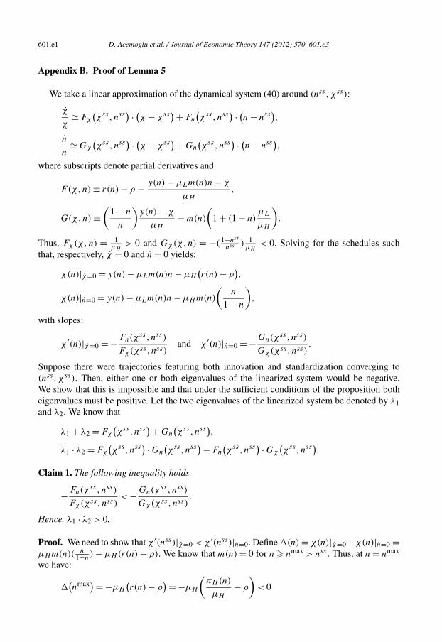
601.e1 D. Acemoglu et al. / Journal of Economic Theory 147 (2012) 570–601.e3

Appendix B. Proof of Lemma 5

We take a linear approximation of the dynamical system (40) around (nss, χss):

χ

χ� Fχ

(χss, nss

) · (χ − χss) + Fn

(χss, nss

) · (n − nss),

n

n� Gχ

(χss, nss

) · (χ − χss) + Gn

(χss, nss

) · (n − nss),

where subscripts denote partial derivatives and

F(χ,n) ≡ r(n) − ρ − y(n) − μLm(n)n − χ

μH

,

G(χ,n) ≡(

1 − n

n

)y(n) − χ

μH

− m(n)

(1 + (1 − n)

μL

μH

).

Thus, Fχ(χ,n) = 1μH

> 0 and Gχ(χ,n) = −( 1−nss

nss ) 1μH

< 0. Solving for the schedules suchthat, respectively, χ = 0 and n = 0 yields:

χ(n)|χ=0 = y(n) − μLm(n)n − μH

(r(n) − ρ

),

χ(n)|n=0 = y(n) − μLm(n)n − μH m(n)

(n

1 − n

),

with slopes:

χ ′(n)|χ=0 = − Fn(χss, nss)

Fχ(χss, nss)and χ ′(n)|n=0 = − Gn(χ

ss, nss)

Gχ(χss, nss).

Suppose there were trajectories featuring both innovation and standardization converging to(nss, χss). Then, either one or both eigenvalues of the linearized system would be negative.We show that this is impossible and that under the sufficient conditions of the proposition botheigenvalues must be positive. Let the two eigenvalues of the linearized system be denoted by λ1and λ2. We know that

λ1 + λ2 = Fχ

(χss, nss

) + Gn

(χss, nss

),

λ1 · λ2 = Fχ

(χss, nss

) · Gn

(χss, nss

) − Fn

(χss, nss

) · Gχ

(χss, nss

).

Claim 1. The following inequality holds

− Fn(χss, nss)

Fχ(χss, nss)< − Gn(χ

ss, nss)

Gχ(χss, nss).

Hence, λ1 · λ2 > 0.

Proof. We need to show that χ ′(nss)|χ=0 < χ ′(nss)|n=0. Define �(n) = χ(n)|χ=0 −χ(n)|n=0 =μH m(n)( n

1−n) − μH (r(n) − ρ). We know that m(n) = 0 for n � nmax > nss. Thus, at n = nmax

we have:

�(nmax) = −μH

(r(n) − ρ

) = −μH

(πH (n) − ρ

)< 0

μH

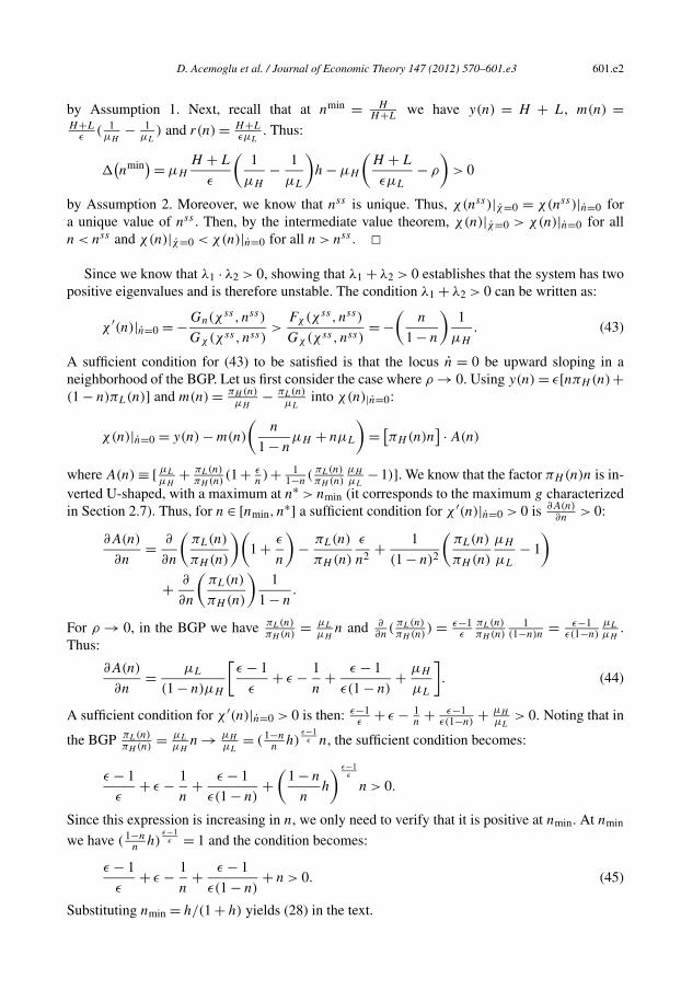
D. Acemoglu et al. / Journal of Economic Theory 147 (2012) 570–601.e3 601.e2

by Assumption 1. Next, recall that at nmin = HH+L

we have y(n) = H + L, m(n) =H+L

ε( 1μH

− 1μL

) and r(n) = H+LεμL

. Thus:

�(nmin) = μH

H + L

ε

(1

μH

− 1

μL

)h − μH

(H + L

εμL

− ρ

)> 0

by Assumption 2. Moreover, we know that nss is unique. Thus, χ(nss)|χ=0 = χ(nss)|n=0 fora unique value of nss . Then, by the intermediate value theorem, χ(n)|χ=0 > χ(n)|n=0 for alln < nss and χ(n)|χ=0 < χ(n)|n=0 for all n > nss. �

Since we know that λ1 · λ2 > 0, showing that λ1 + λ2 > 0 establishes that the system has twopositive eigenvalues and is therefore unstable. The condition λ1 + λ2 > 0 can be written as:

χ ′(n)|n=0 = − Gn(χss, nss)

Gχ(χss, nss)>

Fχ(χss, nss)

Gχ(χss, nss)= −

(n

1 − n

)1

μH

. (43)

A sufficient condition for (43) to be satisfied is that the locus n = 0 be upward sloping in aneighborhood of the BGP. Let us first consider the case where ρ → 0. Using y(n) = ε[nπH (n)+(1 − n)πL(n)] and m(n) = πH (n)

μH− πL(n)

μLinto χ(n)|n=0:

χ(n)|n=0 = y(n) − m(n)

(n

1 − nμH + nμL

)= [

πH (n)n] · A(n)

where A(n) ≡ [ μL

μH+ πL(n)

πH (n)(1+ ε

n)+ 1

1−n(

πL(n)πH (n)

μH

μL−1)]. We know that the factor πH (n)n is in-

verted U-shaped, with a maximum at n∗ > nmin (it corresponds to the maximum g characterizedin Section 2.7). Thus, for n ∈ [nmin, n

∗] a sufficient condition for χ ′(n)|n=0 > 0 is ∂A(n)∂n

> 0:

∂A(n)

∂n= ∂

∂n

(πL(n)

πH (n)

)(1 + ε

n

)− πL(n)

πH (n)

ε

n2+ 1

(1 − n)2

(πL(n)

πH (n)

μH

μL

− 1

)

+ ∂

∂n

(πL(n)

πH (n)

)1

1 − n.

For ρ → 0, in the BGP we have πL(n)πH (n)

= μL

μHn and ∂

∂n(

πL(n)πH (n)

) = ε−1ε

πL(n)πH (n)

1(1−n)n

= ε−1ε(1−n)

μL

μH.

Thus:

∂A(n)

∂n= μL

(1 − n)μH

[ε − 1

ε+ ε − 1

n+ ε − 1

ε(1 − n)+ μH

μL

]. (44)

A sufficient condition for χ ′(n)|n=0 > 0 is then: ε−1ε

+ ε − 1n

+ ε−1ε(1−n)

+ μH

μL> 0. Noting that in

the BGP πL(n)πH (n)

= μL

μHn → μH

μL= ( 1−n

nh)

ε−1ε n, the sufficient condition becomes:

ε − 1

ε+ ε − 1

n+ ε − 1

ε(1 − n)+

(1 − n

nh

) ε−1ε

n > 0.

Since this expression is increasing in n, we only need to verify that it is positive at nmin. At nmin

we have ( 1−nn

h)ε−1ε = 1 and the condition becomes:

ε − 1

ε+ ε − 1

n+ ε − 1

ε(1 − n)+ n > 0. (45)

Substituting nmin = h/(1 + h) yields (28) in the text.

601.e3 D. Acemoglu et al. / Journal of Economic Theory 147 (2012) 570–601.e3

Finally, for n > n∗, rewrite the necessary condition as:

χ ′(n)|n=0

χ(n)|n=0= π ′

H (n)

πH (n)+ 1

n+ ∂A

∂n

1

A> −

(n

1 − n

)1

μH χ(n)|n=0.

From Eqs. (16) and (17):

π ′H (n)

πH (n)+ 1

n= 1

ε

[y(n)] 1−εε

ε − 1

(H

n

) ε−1ε − 1

ε

[y(n)] 1−εε

ε − 1

(L

1 − n

) ε−1ε + 1

nε.

Substituting [y(n)] ε−1ε = (1 − n)

1ε L

ε−1ε + n

1ε H

ε−1ε into this expression, we have

− 1

ε(ε − 1)

(1 − n)−1

1 + ( n1−n

)1ε h

ε−1ε

<π ′

H (n)

πH (n)+ 1

n.

This implies that ∂A(n)∂n

1A(n)

> 1ε(ε−1)

11−n

1+( n1−n

)1ε h

ε−1ε

is a sufficient condition for χ ′(n)|n=0 > 0.

Using (44) and the fact that in BGP πL(n)πH (n)

= μL

μHn, it can be verified that this condition is satis-

fied when (45) holds, for any n ∈ [n∗,1]. In sum, (45) is sufficient to prove that the dynamicalsystem with both innovation and standardization is locally unstable in the limit where ρ → 0. Bycontinuity, the same result applies for ρ < ρ for some ρ > 0 sufficiently small.

Documents

Competing engines of growth: Innovation and standardization