Embed Size (px)
Citation preview
Compensation and Peer Effects in Competing Sales Teams Tat Y. Chan, Jia Li, and Lamar Pierce1
Olin Business School Washington University in St. Louis
Campus Box 1133, One Brookings Drive Saint Louis, MO 63130
May 29, 2009
Abstract. We use Chinese cosmetic sales transaction data to examine how compensation and firm boundaries influence worker productivity spillovers and competition strategies. Implementing improved methodology, we find strong peer effects among workers, demonstrating important new findings. First, we find spillovers are positive under team-based compensation while negative under individual-based compensation. Second, we find peer effects across firm boundaries that depend on compensation system. Third, we find strategic price discounting and customer focus in response to high-ability peers within individual-based counters. Our results suggest that heterogeneity in worker productivity enhances team performance under team-based compensation while hurting individual-based firms.
1 Tat Y. Chan is Associate Professor of Marketing, Jia Li is a doctoral student in Marketing, and Lamar Pierce is Assistant Professor of Strategy, all at Olin Business School, Washington University in St. Louis. Authors can be reached at [email protected], [email protected], or [email protected].
1
1. Introduction
Co-located workers can significantly impact one another’s productivity. These
productivity spillovers may be positive, as coordination improves each worker’s production
through knowledge transfer (e.g. Marshall 1890; Lucas 1988; Berg et al. 1996) and
complementarities in skills and abilities (e.g. Boning et al. 2007; Gant et al. 2002, 2003). Yet
workers may also negatively impact their peers through the reduced effort of free-riding (e.g.
Holmstrom 1979), production externalities from coworkers (e.g. Holmstrom 1982), or
competition between peers under the high-powered incentives of pay-for-performance or
tournament-based compensation (e.g. Lazear and Rosen 1981). Workers in teams may use social
pressure or norms, however, to reduce the cost of free-riding (e.g. Hollander 1990; Kandel and
Lazear 1992; Bernheim 1994). Peer effects may also impact other choices of coworkers
including the allocation of effort among multiple tasks as well as strategic actions such as
discretionary pricing. The many ways in which workers can affect one another provide a simple
yet powerful implication – whom you work with matters.
Recent empirical work has documented peer effects in different work settings (e.g. Ichino
and Maggi 2000; Falk and Ichino 2006; Bandiera et al. 2007; Mas and Moretti 2009), showing
that the quality of peers influences worker behavior and lead to a positive effect of worker
heterogeneity on overall team performance (e.g. Hamilton et al. 2003; Mas and Moretti 2009).
While these results on peer effects are important, they have been observed exclusively within
unique firms or groups and under singular compensation structure. Previous theoretical work
suggests great value in studying peer effects under multiple compensation systems, as the
direction and magnitude of peer effects may be critically linked to the incentives a firm offers to
workers. Kandel and Lazear (1992), for example, show how a partnership structure can provide
incentive to reduce free-riding through peer pressure. Itoh (1991) similarly models how
compensation structure might induce team members to exert effort toward helping one another.
While Holmstrom and Milgrom (1991) present a simple linear model of task allocation in which
it is never optimal for two agents to be jointly responsible for any task, Itoh (1992) finds that
with some modification it is optimal for an agent to help others and hence to be jointly
responsible for each task. Itoh (1993) further develops this theory by showing that principals can
better implement cooperation among agents through team-based incentive systems than through
individual incentives, while acknowledging that such systems also induce additional free-riding.
2
Che and Yoo (2001) further show that repeated interactions of agents in long-term can create
implicit incentives by encouraging employees’ peer sanctioning. The collective implication of
these theories is that team-based compensation may provide positive peer effects by inducing
voluntary cooperative behavior by individual workers.
In this paper we examine an empirical setting – cosmetic sales in a Chinese department
store – which exhibits strong peer effects under different compensation systems. In this store,
multiple manufacturers employ salespeople to work at co-located counters on the retail floor.
Some of these brand-based counters employ team-based compensation (TC) while others use
individual commissions (IC). Salespeople use selling effort, discounting and other discretionary
strategies to compete for customers in the store with other salespeople inside and outside the
counter. We use a detailed three-year dataset that identifies the individual salesperson, prices,
products, and time for each transaction of this period. Such level of detail allows us to build a
peer effects model to study how in each period any worker’s temporal productivity is influenced
by the contemporaneous set of peers within and outside the counter. We allow these peer effects
to depend on the compensation systems adopted by the worker’s own counter and competing
counters. We also allow for asymmetric peer effects where a worker may be influenced
differently by superiors (peers with higher permanent productivity) vs. inferiors (peers with
lower permanent productivity). We use a nested non-linear least squares algorithm to
simultaneously estimate permanent worker productivities and peer effects on concurrently-
scheduled salespeople’s revenue, unit sales, discounting, and customer mix. This method
enables us to study the complicated within-counter and cross-counter peer effects that depend on
the compensation systems of both the focal worker and her peers, and to generate estimators that
are more efficient than the two-step estimators adopted in previous studies.
Our results are generally consistent with previous literature showing productivity
spillovers to coworkers. We find that the direction and magnitude of peer effects are critically
linked to compensation systems. IC counters produce negative peer effects among employees
that suggest within-counter competition. In particular, salespeople are out-competed by superior
peers, yet superior peers do not appear to gain much from lower ability peers. In contrast,
working with superior peers will improve worker productivity in TC counters. These results are
consistent with existing theory (Itoh 1991, 1992, 1993; Kandel and Lazear 1992; Che and Yoo
2001) on how team-based incentives can increase peer cooperation. In fact, our results are
3
difficult to explain without some element of cooperation or helping behaviors. If peer effects
purely come from learning, sales for each worker should stabilize after many months of worker
interactions (unless there was considerable forgetting). This is inconsistent with our findings that
a worker’s temporal productivity is strongly influenced by contemporaneous peers. Another
potential explanation, mimicry or imitation among co-located workers, does not explain why our
estimated peer effects differ across compensation systems. Workers at IC counters are capable
of mimicry as well, yet their negative peer effects show no evidence of this occurring.
Our results are also consistent with existing evidence on worker heterogeneity and
performance, although we demonstrate that this effect is highly dependent on compensation
system. While heterogeneity in worker ability improves team performance at TC counters as in
previous empirical works (e.g. Hamilton et al. 2003; Leonard and Levine 2006; Mas and Moretti
2009), we show that heterogeneity reduces overall sales at IC counters. This implies that the
optimal mix of workers may depend on the firm’s choice of compensation system.
Besides demonstrating results consistent with existing economic theory, our study
generates a set of new findings that leads to several important economic questions unanswered in
the previous literature. First, while previous research on peer effects focuses on productivity
spillovers, workers in the real workplace may actively respond to peers by employing
discretionary strategies to compete with one another. Increased competition from high-ability
peers may induce workers to offer lower prices, both when this competition comes from inside
and outside the firm. Existing empirical literature shows that incentives can lead to employees
gaming the timing and pricing of sales (Oyer 1998; Larkin 2008) and other performance metrics
(Asch 1990; Courty and Marschke 2004) across many industries. Similarly, some agency
literature demonstrates that agents may allocate effort across multiple tasks in ways that are
suboptimal for the principal. Holmstrom and Milgram (1994) and Baker (1992) show that under
task-based piece rates, workers may allocate effort to specific tasks in ways that do not account
for their complementary nature to the principal. Marx and MacDonald (2001) demonstrate that
the magnitude of this “adverse specialization” highly depends on the compensation system
offered to the agents. Our results show that workers at IC counters increase price discounting in
response to high-ability peers within counters and across competing counters. They also respond
by focusing on retaining high-value customers who may be loyal to them and therefore difficult
for peers to steal. However, we find that workers at TC counters do not discount prices in
4
response to high-ability peers; instead, they may choose to coordinate in task allocation. High-
ability workers may let lower-ability peers serve high-value customers who may be loyal to their
brands, while they focus on competing for new customers who may have lower transaction value
and are difficult to attract. In the end overall counter sales improves, which is evidenced from
our finding that heterogeneity in worker ability improves team performance at TC counters.
Second, the importance of peer effects may extend beyond the firm boundaries to other
organizations through competition. When two competing sales teams are co-located, for
example, the high-ability workers in a team are more likely to steal business from the competing
team than are low-ability peers. Their competitiveness may also depend on the compensation
systems adopted by the teams. We find that high-ability workers at IC counters are less likely to
impact outside peers, since the focus of their effort is on competing with inside peers. In
contrast, high-ability workers at TC counters have strong negative effects on outside peers, as
they can exert the entirety of their effort toward cross-counter competition. Our results suggest
that, while individual compensation may motivate workers, it also transfers much of their
competitive effort to within the firm. This may reduce the firm’s ability to compete with rivals,
and when combined with employees’ pricing discretion, may lead to lower profit as well. While
data constraints limit our ability to determine whether one compensation system dominates
another in profitability, our results suggest that TC produces coordination gains that improve a
firm’s responsiveness to competition, which will reduce the impact of star salespeople in
competing brands.
This paper provides a unique contribution to the personnel economics literature by
simultaneously estimating peer effects on productivity both within and across firms under
multiple compensation systems. It is also the first to study peer effects under discretionary
pricing, contributing to the literature on employee gaming behaviors. Our results have important
implications for managers of sales groups as well as those providing the marketplaces in which
they compete. For instance, we show that worker diversity of skills affects team productivity
and competitiveness differently under different compensation systems, a finding that should be
important to those studying personnel and organizational economics.
5
2. Cosmetic Sales in a Chinese Department Store
We study peer effects in the context of team cosmetic sales in a department store in a
large metropolitan area in Eastern China. This department store is one of the largest in China in
both sales and profit, and sells a wide range of products including apparel, jewelry, watches,
home furnishings, appliances, electronics, toys, and food. One of its largest categories is
cosmetics, the fifth largest consumer market in China with annual sales of $85 billion in 2004.2
The department store has 15 major brands in the cosmetics department, with each occupying a
counter in the same floor area. These brands hire their own workers to promote and sell their
products, while paying the department store a share of their revenues. The cosmetics floor
effectively becomes an open market, with multiple firms competing for customers in a shared
space. The department store manages the arrangement of the counters as well as the staffing of
the manufacturers’ employees in shifts. We observe each individual cosmetic sale for 11 of the
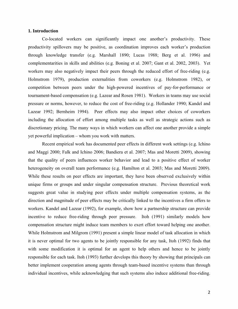
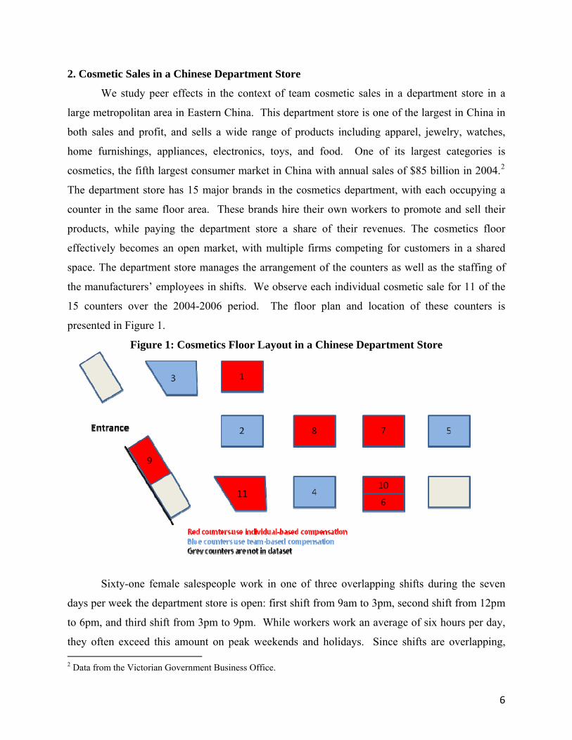
15 counters over the 2004-2006 period. The floor plan and location of these counters is
presented in Figure 1.
Figure 1: Cosmetics Floor Layout in a Chinese Department Store
Sixty-one female salespeople work in one of three overlapping shifts during the seven
days per week the department store is open: first shift from 9am to 3pm, second shift from 12pm
to 6pm, and third shift from 3pm to 9pm. While workers work an average of six hours per day,
they often exceed this amount on peak weekends and holidays. Since shifts are overlapping, 2 Data from the Victorian Government Business Office.
6
workers need not work the same shift in a given day to share the counter. Salespeople typically
rotate shifts that are assigned by the department store manager. For example, if a salesperson
works in the first shift on Monday, she will typically work in the second or third shift on
Tuesday. This scheduling process, while not completely random, ensures that each salesperson
will rotate workdays and times, and thereby share their shifts with a variety of their peers. In
interviews with the department store manager, we learned that there was no strategic scheduling
of workers with either certain peers or during specific shifts or days of the week.
One of the interesting aspects of this store is that the individual brands use two different
compensation systems: team-based commissions (TC) and individual-based commissions (IC).
The four brands using TC pay each worker based on a tiered percentage of the monthly total
counter sales. As sales increase, the percentage commission grows. If payments were calculated
daily, then workers might decide how much to free-ride each day based on the expected
productivity of their concurrently-scheduled workers. But since pay is calculated monthly and
worker staffing over the month is equally distributed, each worker’s compensation is based
approximately equally on each peer working that month. This means that on any day, the
financial motivation for free-riding on coworkers should remain independent of concurrently-
scheduled peers. Still, with whom a worker works may be important since coordination,
specialization, and learning may make skilled coworkers a boon for own individual sales.
Furthermore, as shown in Mas and Moretti (2009), working with superior workers may create a
peer pressure that can reduce the extent of free-riding even without financial motivation.
The other seven brands that we observe use individual-based commissions.3 In these
counters, individual output is recorded and workers are compensated based on an increasing
tiered percentage of personal monthly sales.4 IC counters do not suffer from problems of free-
riding, but may suffer instead from two afflictions. First, despite representing the same brand,
coworkers are incentivized to directly compete with one another for customers, rather than with
competing counters. Second, workers have little incentive to coordinate with or help peers, or to
work to reduce negative production externalities within the counter. Thus, in IC counters whom
you work with also matters, because they represent your competition and the source of
production externalities. 3 In the case of cosmetics sales, individual workers are technologically independent, and precise measures of individual sales are possible. 4 The four counters for which we do not have sales data also use individual-based compensation.
7
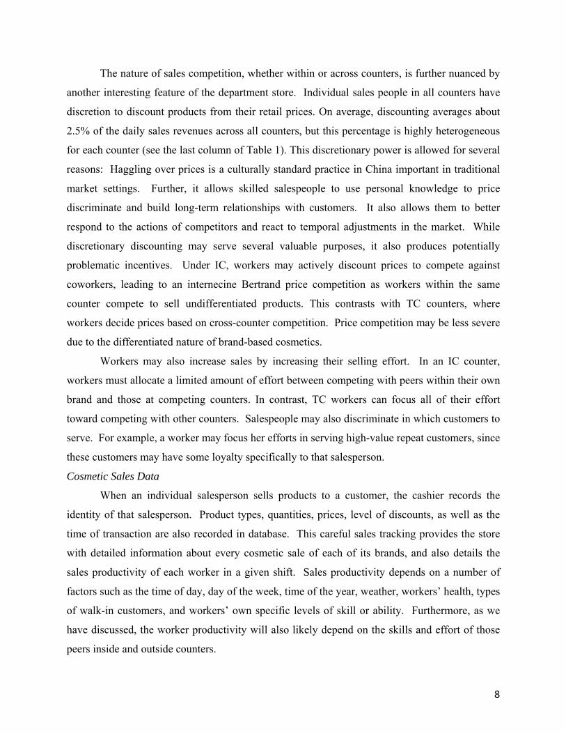
The nature of sales competition, whether within or across counters, is further nuanced by
another interesting feature of the department store. Individual sales people in all counters have
discretion to discount products from their retail prices. On average, discounting averages about
2.5% of the daily sales revenues across all counters, but this percentage is highly heterogeneous
for each counter (see the last column of Table 1). This discretionary power is allowed for several
reasons: Haggling over prices is a culturally standard practice in China important in traditional
market settings. Further, it allows skilled salespeople to use personal knowledge to price
discriminate and build long-term relationships with customers. It also allows them to better
respond to the actions of competitors and react to temporal adjustments in the market. While
discretionary discounting may serve several valuable purposes, it also produces potentially
problematic incentives. Under IC, workers may actively discount prices to compete against
coworkers, leading to an internecine Bertrand price competition as workers within the same
counter compete to sell undifferentiated products. This contrasts with TC counters, where
workers decide prices based on cross-counter competition. Price competition may be less severe
due to the differentiated nature of brand-based cosmetics.
Workers may also increase sales by increasing their selling effort. In an IC counter,
workers must allocate a limited amount of effort between competing with peers within their own
brand and those at competing counters. In contrast, TC workers can focus all of their effort
toward competing with other counters. Salespeople may also discriminate in which customers to
serve. For example, a worker may focus her efforts in serving high-value repeat customers, since
these customers may have some loyalty specifically to that salesperson.
Cosmetic Sales Data
When an individual salesperson sells products to a customer, the cashier records the
identity of that salesperson. Product types, quantities, prices, level of discounts, as well as the
time of transaction are also recorded in database. This careful sales tracking provides the store
with detailed information about every cosmetic sale of each of its brands, and also details the
sales productivity of each worker in a given shift. Sales productivity depends on a number of
factors such as the time of day, day of the week, time of the year, weather, workers’ health, types
of walk-in customers, and workers’ own specific levels of skill or ability. Furthermore, as we
have discussed, the worker productivity will also likely depend on the skills and effort of those
peers inside and outside counters.
8
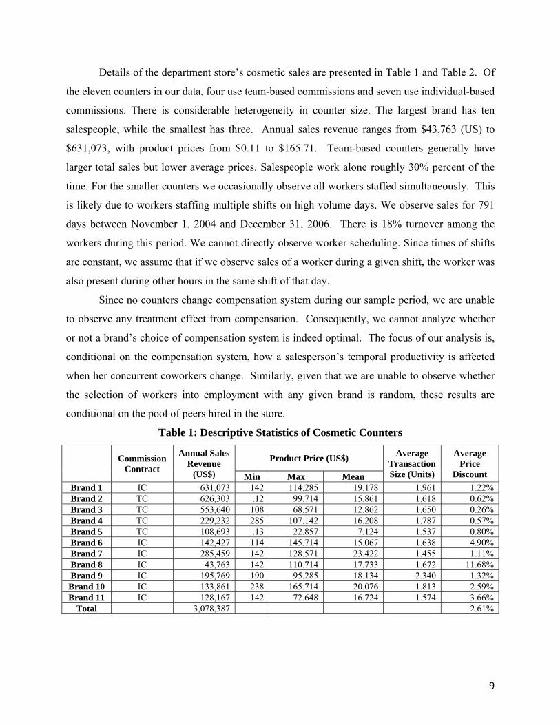
Details of the department store’s cosmetic sales are presented in Table 1 and Table 2. Of
the eleven counters in our data, four use team-based commissions and seven use individual-based
commissions. There is considerable heterogeneity in counter size. The largest brand has ten
salespeople, while the smallest has three. Annual sales revenue ranges from $43,763 (US) to
$631,073, with product prices from $0.11 to $165.71. Team-based counters generally have
larger total sales but lower average prices. Salespeople work alone roughly 30% percent of the
time. For the smaller counters we occasionally observe all workers staffed simultaneously. This
is likely due to workers staffing multiple shifts on high volume days. We observe sales for 791
days between November 1, 2004 and December 31, 2006. There is 18% turnover among the
workers during this period. We cannot directly observe worker scheduling. Since times of shifts
are constant, we assume that if we observe sales of a worker during a given shift, the worker was
also present during other hours in the same shift of that day.
Since no counters change compensation system during our sample period, we are unable
to observe any treatment effect from compensation. Consequently, we cannot analyze whether
or not a brand’s choice of compensation system is indeed optimal. The focus of our analysis is,
conditional on the compensation system, how a salesperson’s temporal productivity is affected
when her concurrent coworkers change. Similarly, given that we are unable to observe whether
the selection of workers into employment with any given brand is random, these results are
conditional on the pool of peers hired in the store.
Table 1: Descriptive Statistics of Cosmetic Counters
Commission Contract
Annual Sales Revenue
(US$)
Product Price (US$) Average Transaction Size (Units)
Average Price
Discount Min Max Mean Brand 1 IC 631,073 .142 114.285 19.178 1.961 1.22% Brand 2 TC 626,303 .12 99.714 15.861 1.618 0.62% Brand 3 TC 553,640 .108 68.571 12.862 1.650 0.26% Brand 4 TC 229,232 .285 107.142 16.208 1.787 0.57% Brand 5 TC 108,693 .13 22.857 7.124 1.537 0.80% Brand 6 IC 142,427 .114 145.714 15.067 1.638 4.90% Brand 7 IC 285,459 .142 128.571 23.422 1.455 1.11% Brand 8 IC 43,763 .142 110.714 17.733 1.672 11.68% Brand 9 IC 195,769 .190 95.285 18.134 2.340 1.32% Brand 10 IC 133,861 .238 165.714 20.076 1.813 2.59% Brand 11 IC 128,167 .142 72.648 16.724 1.574 3.66%
Total 3,078,387 2.61%
9
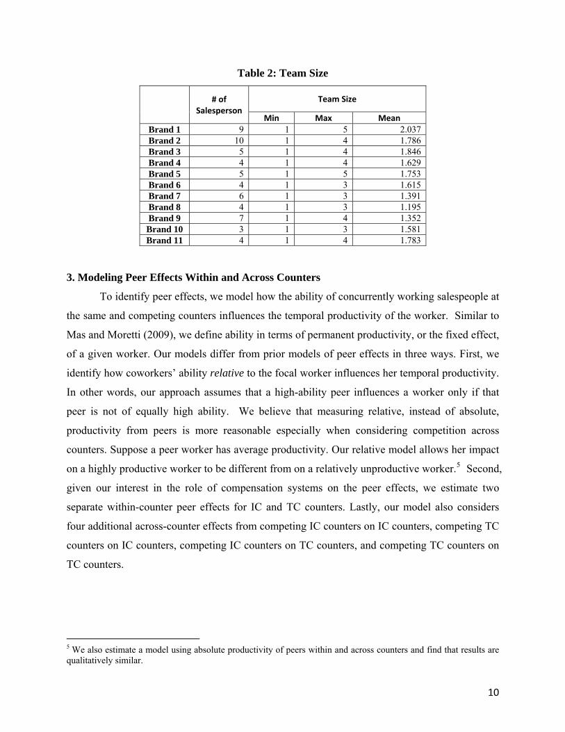
Table 2: Team Size
# of Salesperson
Team Size
Min Max Mean Brand 1 9 1 5 2.037 Brand 2 10 1 4 1.786 Brand 3 5 1 4 1.846 Brand 4 4 1 4 1.629 Brand 5 5 1 5 1.753 Brand 6 4 1 3 1.615 Brand 7 6 1 3 1.391 Brand 8 4 1 3 1.195 Brand 9 7 1 4 1.352 Brand 10 3 1 3 1.581 Brand 11 4 1 4 1.783
3. Modeling Peer Effects Within and Across Counters
To identify peer effects, we model how the ability of concurrently working salespeople at
the same and competing counters influences the temporal productivity of the worker. Similar to
Mas and Moretti (2009), we define ability in terms of permanent productivity, or the fixed effect,
of a given worker. Our models differ from prior models of peer effects in three ways. First, we
identify how coworkers’ ability relative to the focal worker influences her temporal productivity.
In other words, our approach assumes that a high-ability peer influences a worker only if that
peer is not of equally high ability. We believe that measuring relative, instead of absolute,
productivity from peers is more reasonable especially when considering competition across
counters. Suppose a peer worker has average productivity. Our relative model allows her impact
on a highly productive worker to be different from on a relatively unproductive worker.5 Second,
given our interest in the role of compensation systems on the peer effects, we estimate two
separate within-counter peer effects for IC and TC counters. Lastly, our model also considers
four additional across-counter effects from competing IC counters on IC counters, competing TC
counters on IC counters, competing IC counters on TC counters, and competing TC counters on
TC counters.
5 We also estimate a model using absolute productivity of peers within and across counters and find that results are qualitatively similar.
10
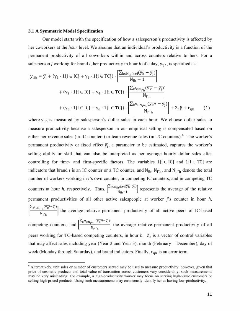
3.1 A Symmetric Model Specification
Our model starts with the specification of how a salesperson’s productivity is affected by
her coworkers at the hour level. We assume that an individual’s productivity is a function of the
permanent productivity of all coworkers within and across counters relative to hers. For a
s esp i f , y , is specified as: al erson j working for brand , her productivity in hour h o a day
y y γ · 1 i IC γ · 1 i TC ·∑ y yN ;
N 1
γ · 1 i IC γ · 1 i TC ·∑ y yN
N
γ · 1 i IC γ · 1 i TC ·∑ y yN
N Z β ε 1
where y is measured by salesperson’s dollar sales in each hour. We choose dollar sales to
measure productivity because a salesperson in our empirical setting is compensated based on
either her revenue sales (in IC counters) or team revenue sales (in TC counters).6 The worker’s
permanent productivity or fixed effect y , a parameter to be estimated, captures the worker’s
selling ability or skill that can also be interpreted as her average hourly dollar sales after
controlling for time- and firm-specific factors. The variables 1 i IC and 1 i TC are
indicators that brand i is an IC counter or a TC counter, and N , N , and N denote the total
number of workers working in i’s own counter, in competing IC counters, and in competing TC
counters at hour h, respectively. Thus, ∑ N ;
N represents the average of the relative
permanent productivities of all other active salespeople at worker j’s counter in hour h, ∑ N
N the average relative permanent productivity of all active peers of IC-based
competing counters, and ∑ N
N the average relative permanent productivity of all
peers working for TC-based competing counters, in hour h. Zh is a vector of control variables
that may affect sales including year (Year 2 and Year 3), month (February – December), day of
week (Monday through Saturday), and brand indicators. Finally, ε is an error term.
6 Alternatively, unit sales or number of customers served may be used to measure productivity; however, given that price of cosmetic products and total value of transaction across customers vary considerably, such measurements may be very misleading. For example, a high-productivity worker may focus on serving high-value customers or selling high-priced products. Using such measurements may erroneously identify her as having low-productivity.
11
Peer effects in equation (1) are captured by the parameters γ’s. Parameters γ1 and γ2
represent the within-counter peer effects for IC and TC counters, respectively. γ3 and γ4 measure
the peer effects from workers at IC-based competing counters on salespeople at IC and TC
counters, respectively. γ5 and γ6 measure the peer effects from peers who work at TC-based
competing counters on salespeople at IC and TC counters, respectively. Because the model
restricts γ’s to be the same for peer effects from superiors as from inferiors, we call this a
“symmetric” model.
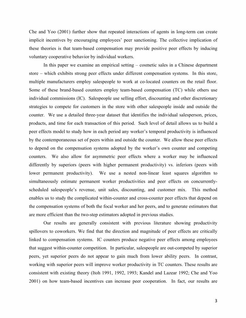
Figure 2 provides a visual representation of the peer effects for four competing counters
taken from Figure 1.7 We represent the peer effects on two focal workers, worker A from
counter 2 and worker B from counter 8, from both within and across counters. Blue represents
TC counters, while red represents IC counters. Arrows from each worker to the focal workers
represent the peer effects based on the permanent productivity of the eight workers. For worker
A at TC counter, her peer effects are measured by γ2 from a within-counter coworker, γ4 from the
average relative productivity of four other co-workers from competing IC counters, and γ6 from
the average relative productivity of two other coworkers from competing TC counters. Similarly
the peer effects on worker B at IC counter are measured by γ1, γ3, and γ5.
7 A counter is defined as “competing” if it is adjacent to the counter of worker j in any direction. For example, counter 1 in Figure 1 would have three competing counters: 2, 3, and 8. We include only adjacent competing counters in all our models. Alternative models with distant competing counters show consistent results, with cross-counter peer effects diminishing with distance between counters.
12
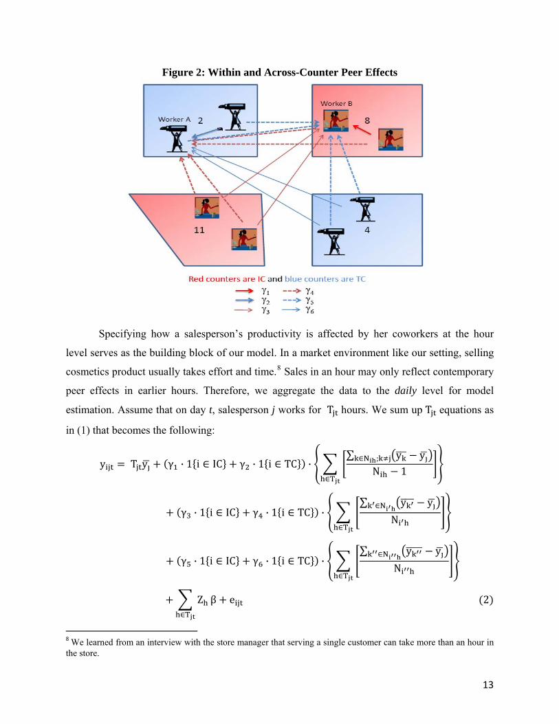
Figure 2: Within and Across-Counter Peer Effects
Specifying how a salesperson’s productivity is affected by her coworkers at the hour
level serves as the building block of our model. In a market environment like our setting, selling
cosmetics product usually takes effort and time.8 Sales in an hour may only reflect contemporary
peer effects in earlier hours. Therefore, we aggregate the data to the daily level for model
estimation. Assume that on day t, salesperson j works for T hours. We sum up T equations as
in (1) that becomes the following:
y T y γ · 1 i IC γ · 1 i TC ·∑ y yN ;
N 1T
γ · 1 i IC γ · 1 i TC ·∑ y yN
NT
γ · 1 i IC γ · 1 i TC ·∑ y yN
NT
ZT
β e 2
8 We learned from an interview with the store manager that serving a single customer can take more than an hour in the store.
13
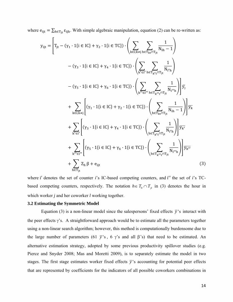
where e ∑ εT . With simple algebraic manipulation, equation (2) can be re-written as:
y T γ · 1 i IC γ · 1 i TC ·1
N 1T T;
γ · 1 i IC γ · 1 i TC ·1N
T T
γ · 1 i IC γ · 1 i TC ·1
NT T
y
γ · 1 i IC γ · 1 i TC ·1
N 1T T
y;
γ · 1 i IC γ · 1 i TC ·1N
T T
y
γ · 1 i IC γ · 1 i TC ·1
N yT T
ZT
β e 3
where i denotes the set of counter i’s IC-based competing counters, and i the set of i’s TC-
based competing counters, respectively. The notation lt jth T T∈ ∩ in (3) denotes the hour in
which worker j and her coworker l working together.
3.2 Estimating the Symmetric Model
Equation (3) is a non-linear model since the salespersons’ fixed effects 'sy interact with
the peer effects γ’s. A straightforward approach would be to estimate all the parameters together
using a non-linear search algorithm; however, this method is computationally burdensome due to
the large number of parameters (61 'sy , 6 γ’s and all β’s) that need to be estimated. An
alternative estimation strategy, adopted by some previous productivity spillover studies (e.g.
Pierce and Snyder 2008; Mas and Moretti 2009), is to separately estimate the model in two
stages. The first stage estimates worker fixed effects 'sy accounting for potential peer effects
that are represented by coefficients for the indicators of all possible coworkers combinations in
14
data; in the second stage the estimated fixed effects are plugged into a counterpart of equation (3)
in our model to estimate the γ’s. While this method is simple to implement, applying it to our
context raises an efficiency issue. The data requirement to estimate the first stage is very high,
since it models the peer effects of all possible combinations of coworkers, within and across
counters using a non-parametric approach. Because we only have a limited number of repeat
observations for many coworker combinations in our data, we expect the estimates in the first
stage to be very imprecise if we apply this method.
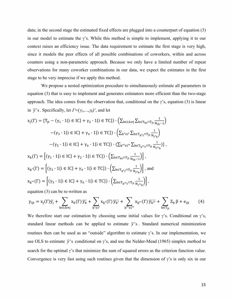
We propose a nested optimization procedure to simultaneously estimate all parameters in
equation (3) that is easy to implement and generates estimators more efficient than the two-stage
approach. The idea comes from the observation that, conditional on the γ’s, equation (3) is linear
in 'sy . Specif ca , let Γ=(γ ,…, )’, and let
x Γ T ·
i lly 1 γ6
γ · 1 i IC γ · 1 i TC ∑ ∑N;
N
T T
γ · 1 i IC γ · 1 i TC · ∑ ∑ T
∑ ∑N
T
γ · 1 i IC γ · 1 i TC · T
· ·N
T ,
x Γ γ 1 i IC γ 1 i TC · ∑
· · ·N
T T ,
x Γ γ 1 i IC γ 1 i TC ∑ ,
x Γ γ · 1 i IC γ · 1 i TC · ∑N
T T and
T T ,
e ua eq tion (3) can b re-written as
y x Γ y x Γ;
y x Γ y x Γ y ZT
β e 4
We therefore start our estimation by choosing some initial values for γ’s. Conditional on γ’s,
standard linear methods can be applied to estimate 'sy . Standard numerical minimization
routines then can be used as an “outside” algorithm to estimate γ’s. In our implementation, we
use OLS to estimate 'sy conditional on γ’s, and use the Nelder-Mead (1965) simplex method to
search for the optimal γ’s that minimize the sum of squared errors as the criterion function value.
Convergence is very fast using such routines given that the dimension of γ’s is only six in our
15
model. Finally, we compute robust standard errors for our estimated parameters accounting for
the existence of heteroscedasticity in error terms eijt.9
3.3 Model Identification
Since none of the counters change pay policies during the period of our data, we are
unable to identify how a change in compensation system can alter worker behavior. In contrast,
the combination of workers during any given shift varies. High-ability workers are sometimes
scheduled with other high-ability workers and sometimes with low-ability peers. We use this
variation in the mix of co-scheduled workers to identify short term peer effects on individual and
team productivity under different compensation systems.
This identification strategy relies on the assumption that workers are distributed
approximately randomly with their peers, that is, high-ability workers have equal chance to be
scheduled with low-ability and high-ability peers. While interviews with management suggest
that worker assignment is independent of ability, we verify this by using a chi-squared test to test
the hypothesis that all worker pairings are equally frequent. We separately identify all possible
coworker pairings for each counter in every month, and compare the number of times each pair
of worker working together with the expected number of times under the null hypothesis of
random shift assignments. Table 3 presents the results, showing that we are unable to reject this
null hypothesis at the 10% significance level for any counter, supporting our assertion that
workers are not systematically scheduled based on ability.
One might still be concerned that team formation varies across the time of a day. For
example, more productive workers may be systematically scheduled to work together when
demand spikes upwards. To test this hypothesis we follow Mas and Moretti (2009) to examine
the relationship between the number of personnel on duty and the average ability of workers. A
positive relationship between the change in personnel and the change in average permanent
productivity of workers may suggest that higher ability workers will add to the shift when
demand is high. We compare this relationship across consecutive 1-hour periods for each counter,
and find little change in the average permanent productivity when the number of workers
9 An implicit assumption of our symmetric model specification is that the number of coworkers on duty does not affect how team members interact with one another. In an alternative specification, we relax this assumption by adding a power term α to capture the possible effect of team size on productivity spillovers. The estimate of α is close to one, suggesting that the size of coworkers plays little role in the magnitude of peer effects.
16
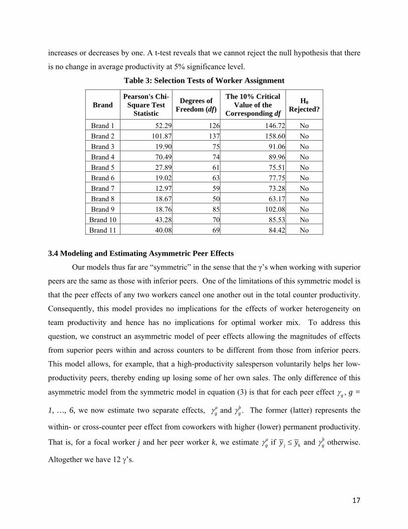
increases or decreases by one. A t-test reveals that we cannot reject the null hypothesis that there
is no change in average productivity at 5% significance level.
Table 3: Selection Tests of Worker Assignment
Pearson's Chi-Square Test
Statistic
The 10% Critical Value of the
Corresponding df Degrees of
Freedom (df)H0
Rejected? Brand
Brand 1 No 52.29 126 146.72Brand 2 No 101.87 137 158.60Brand 3 No 19.90 75 91.06Brand 4 No 70.49 74 89.96Brand 5 No 27.89 61 75.51Brand 6 No 19.02 63 77.75Brand 7 No 12.97 59 73.28Brand 8 No 18.67 50 63.17Brand 9 No 18.76 85 102.08Brand 10 No 43.28 70 85.53Brand 11 No 40.08 69 84.42
3.4 Modeling and Estimating Asymmetric Peer Effects
Our models thus far are “symmetric” in the sense that the γ’s when working with superior
peers are the same as those with inferior peers. One of the limitations of this symmetric model is
that the peer effects of any two workers cancel one another out in the total counter productivity.
Consequently, this model provides no implications for the effects of worker heterogeneity on
team productivity and hence has no implications for optimal worker mix. To address this
question, we construct an asymmetric model of peer effects allowing the magnitudes of effects
from superior peers within and across counters to be different from those from inferior peers.
This model allows, for example, that a high-productivity salesperson voluntarily helps her low-
productivity peers, thereby ending up losing some of her own sales. The only difference of this
asymmetric model from the symmetric model in equation (3) is that for each peer effect gγ , g =
1, …, 6, we now estimate two separate effects, agγ b
gγ and . The former (latter) represents the
within- or cross-counter peer effect from coworkers with higher (lower) permanent productivity.
That is, for a focal worker j and her peer worker k, we estimate agγ b
gγ if j ky y≤ and otherwise.
Altogether we have 12 γ’s.
17
Though the extension is straightforward, our nested non-linear estimation algorithm
cannot be directly applied to this model. The key of using the algorithm is that all permanent
productivity parameters 'y s are linear conditional on γ’s. With asymmetric effects, however,
'y s now interact with indicator functions { }j ky y≤ { }j ky y> or , where k . To avoid
estimating non-linearly all 61
j≠
'y s in our model we employ another trick in model estimation.
Notice that to construct the indicators { }j ky y≤ { }j ky y> or , all we need is the productivity
ranking for workers j and k. Suppose we use the ranking of workers’ average sales observed in
the data to proxy the ranking of permanent productivities. These two rankings should be
consistent with each other if peer effects do not dominate permanent productivity10 and the shifts
of workers are truly randomly assigned. If there is any inconsistency in the rankings this may
indicate the existence of systematic selection issues in shift allocation.
In model estimation we use the average daily sales for all salespeople during the
sample period to construct or as a proxy for indicator
y
{ }j ky y≤ or
{ }j ky y> . Conditional on the ranking, we repeat the nested non-linear algorithm as discussed
before to estimate the 12 γ’s and other parameters. Then we compare the ranking of the 'y s
estimated from this procedure with the ranking of . We find that the two rankings are
perfectly consistent with each other, which provides another validity support that there is no
systematic selection issue in shift allocation. To ensure that our estimates are indeed the unique
optima that minimize the criterion function value, we follow up with estimating the whole non-
linear equation system for all γ’s and
ˆ 'y s
'y s . There we employ the Nelder-Meade simplex method
using the estimates we have obtained as initial values. We find the simplex always converges to
the initial values, showing that our estimates are not just local optima. Since our initial values
start at the minima, convergence in this trial exercise is very fast requiring only a few iterations.
4. Estimation Results
Table 4 reports the estimated peer effects from both the symmetric and asymmetric
models. We first present the results of our symmetric model, which identify key differences in
10 In equation (3) this means that the absolute value of γ’s applicable to any worker is much smaller than 1.
18
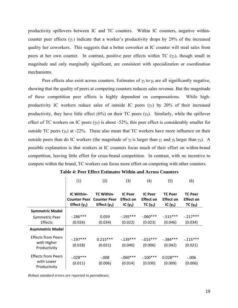
productivity spillovers between IC and TC counters. Within IC counters, negative within-
counter peer effects (γ1) indicate that a worker’s productivity drops by 29% of the increased
quality her coworkers. This suggests that a better coworker at IC counter will steal sales from
peers at her own counter. In contrast, positive peer effects within TC (γ2), though small in
magnitude and only marginally significant, are consistent with specialization or coordination
mechanisms.
Peer effects also exist across counters. Estimates of γ3 to γ6 are all significantly negative,
showing that the quality of peers at competing counters reduces sales revenue. But the magnitude
of these competition peer effects is highly dependent on compensations. While high-
productivity IC workers reduce sales of outside IC peers (γ3) by 20% of their increased
productivity, they have little effect (6%) on their TC peers (γ4). Similarly, while the spillover
effect of TC workers on IC peers (γ5) is about -52%, this peer effect is considerably smaller for
outside TC peers (γ6) at -22%. These also mean that TC workers have more influence on their
outside peers than do IC workers (the magnitude of γ5 is larger than γ3 and γ6 larger than γ4). A
possible explanation is that workers at IC counters focus much of their effort on within-brand
competition, leaving little effort for cross-brand competition. In contrast, with no incentive to
compete within the brand, TC workers can focus more effort on competing with other counters.
Table 4: Peer Effect Estimates Within and Across Counters
(1) (5) (2) (3) (4) (6)
IC Within‐Counter Peer Effect (γ1)
TC Within‐Counter Peer Effect (γ2)
TC Peer Effect on TC (γ6)
IC Peer Effect on IC (γ3)
IC Peer Effect on TC (γ4)
TC Peer Effect on IC (γ5)
Symmetric Model ‐.286*** ‐.515*** 0.059 ‐.195*** ‐.060*** ‐.217***Symmetric Peer
Effects (0.026) (0.046) (0.034) (0.022) (0.023) (0.034)
Asymmetric Model
Effects from Peers with Higher Productivity
‐.197*** ‐.384*** 0.215*** ‐.139*** ‐.015*** ‐.115***(0.018) (0.042) (0.021) (0.040) (0.006) (0.021)
Effects from Peers with Lower Productivity
‐.028*** 0.028*** ‐.008 ‐.060*** ‐.100*** ‐.006(0.011) (0.009) (0.006) (0.014) (0.030) (0.006)
Robust standard errors are reported in parentheses.
19
The last two rows in Table 4 present the peer effects estimated from the asymmetric
model. A positive coefficient from superior peers means improving productivity as it measures
the impact from the positive difference between peers and the focal worker. A positive
coefficient from inferior peers means reducing productivity (the negative difference between the
peer and the focal worker). Again we find considerable differences in both within- and across-
counter peer effects across compensation systems. We also find significant asymmetry in the
peer effects from superior- and inferior-ability coworkers. The first column shows that within IC
counters superior coworkers significantly reduce the sales of an inferior worker (-.197), while
inferior coworkers have a much smaller effect in increasing the performance of a superior worker
(-.028). The second column shows a very different story for peer effects within TC counters.
While inferiors have little effect on their peers, superiors dramatically help peer revenue (.215).11
This result implies that high-ability workers may choose to aid their low-ability peers. Existing
theory suggests two reasons for why high-ability workers might be helping peers. It could be
cooperation among self-interested agents if the monetary reward through enhanced team
performance dominates the cost of her effort (Itoh 1991, 1992, 1993). Additionally, team-pay
may generate an effort-enhancing norm and thus give high-ability workers an incentive to
monitor one another via peer pressure (Kandel and Lazear 1992). Either way, workers’
productivity at TC counters is enhanced through positive spillovers from superior peers. While
our results for IC and TC counters go in opposite directions, both of them are consistent with
previous empirical finding that low productivity workers are more responsive to peer influences
than high productivity workers (e.g. Hamilton et al. 2003; Mas and Moretti 2009).
Cross-counter results are consistent with our symmetric model. The third column shows
that sales of IC workers are negatively impacted by superiors at other IC counters (-.139), while
the fourth column shows that high-ability workers at IC counters have little impact on TC
counters (-.015). Conversely, low-ability IC workers yield larger gains to competing TC counters
(-.100) than to competing IC counters (-.060). Similarly, the fifth column shows strong
competitive peer effects of TC superiors on IC counters (-.384). Enigmatically, TC inferiors
appear to hurt IC revenue (.028), although this coefficient is very small. The resistance to high-
ability peers is also evident in competition between TC counters, as its magnitude (-.115) is 11 This result is in line with the magnitudes found in Falk and Ichino (2006) and Mas and Moretti (2009), where a 10% increase in the average permanent productivity of coworkers increases a given worker’s effort by 1.7% and 1.5%, respectively.
20
significantly smaller than the competitive peer effects of TC superiors on IC counters. These
results suggest that high-ability workers at TC counters have stronger cross-counter peer effects
than their IC counterparts, and that TC counters are less vulnerable to high-ability outside peers
than IC counters.
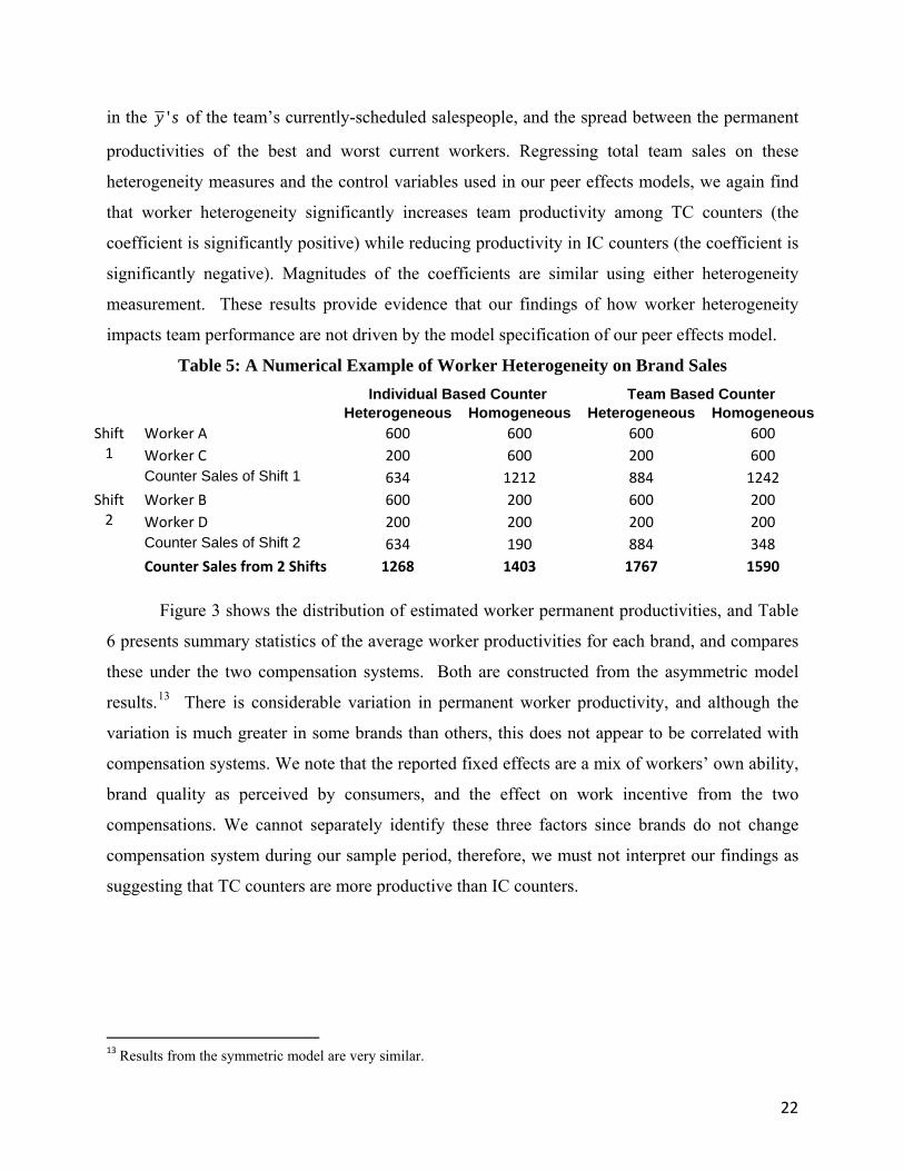
Using the estimation results from the asymmetric model, we conduct a numerical
exercise based on the four-counter context illustrated in Figure 2. The purpose of this exercise is
to illustrate the implications of worker heterogeneity on brand sales. We assume that each of the
four counters has four salespeople that must be allocated across two shifts. Salespeople of all of
the counters except one have the same permanent productivity at 400. The remaining counter has
two high-ability workers, A and B, with permanent productivity of 600 and two low-ability
workers, C and D, with permanent productivity of 200. We consider two scenarios. In the first
scenario, the focal counter uses heterogeneous staffing where one high-ability worker and one
low-ability worker work each shift. In the second scenario, the counter uses homogenous staffing
where the high-ability workers work with one another. Within each scenario, we further look at
two cases: where the focal counter is IC and where it is TC.
Table 5 reports the calculated dollar sales for the focal counter in each scenario. Worker
heterogeneity hurts IC counters, reducing sales from $1403 with homogeneous staffing to $1268
with heterogeneous staffing (10 percent). In contrast, TC counters benefit from heterogeneity.
Although sales in shift 1 when two high productivity coworkers are together generate higher
sales, total counter sales from the two shifts increase from $1590 with homogeneous staffing to
$1769 with heterogeneous staffing (11 percent). The results on heterogeneity in team-based
compensation are consistent with those of Hamilton et al. (2003), but the opposite results on IC
teams show that benefits from heterogeneity are highly dependent on the compensation scheme.
The latter finding is consistent with result in Lazear (1989), suggesting that under certain
conditions “aggressors” should be separated from “non-aggressors” in a team.
For robustness, we employ an additional test of the effect of worker heterogeneity on
team performance. We first identify team sales for each three-hour period12 in our data and,
using the permanent productivities 'y s estimated from our model, calculate each team’s
heterogeneity during that period. We measure heterogeneity in two ways: the standard deviation
12 This is because the combination of coworkers changes in every three-hour period due to the overlaps of the three shifts in a day.
21
in the 'y s of the team’s currently-scheduled salespeople, and the spread between the permanent
productivities of the best and worst current workers. Regressing total team sales on these
heterogeneity measures and the control variables used in our peer effects models, we again find
that worker heterogeneity significantly increases team productivity among TC counters (the
coefficient is significantly positive) while reducing productivity in IC counters (the coefficient is
significantly negative). Magnitudes of the coefficients are similar using either heterogeneity
measurement. These results provide evidence that our findings of how worker heterogeneity
impacts team performance are not driven by the model specification of our peer effects model.
Table 5: A Numerical Example of Worker Heterogeneity on Brand Sales Individual Based Counter Team Based Counter Heterogeneous Homogeneous Heterogeneous Homogeneous
Worker A 600 Shift 1
600 600 600Worker C 200 200 600 600
884 Counter Sales of Shift 1 634 1212 1242Worker B 600 Shift
2 600 200 200
Worker D 200 200 200 200 884 Counter Sales of Shift 2 634 190 348
Counter Sales from 2 Shifts 1767 1268 1403 1590
Figure 3 shows the distribution of estimated worker permanent productivities, and Table
6 presents summary statistics of the average worker productivities for each brand, and compares
these under the two compensation systems. Both are constructed from the asymmetric model
results.13 There is considerable variation in permanent worker productivity, and although the
variation is much greater in some brands than others, this does not appear to be correlated with
compensation systems. We note that the reported fixed effects are a mix of workers’ own ability,
brand quality as perceived by consumers, and the effect on work incentive from the two
compensations. We cannot separately identify these three factors since brands do not change
compensation system during our sample period, therefore, we must not interpret our findings as
suggesting that TC counters are more productive than IC counters.
13 Results from the symmetric model are very similar.
22
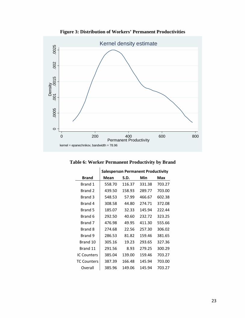
Figure 3: Distribution of Workers’ Permanent Productivities
0.0
005
.001
.001
5.0
02.0
025
Den
sity
0 200 400 600 800Permanent Productivity
kernel = epanechnikov, bandwidth = 78.96
Kernel density estimate
Table 6: Worker Permanent Productivity by Brand
Salesperson Permanent Productivity
Brand Mean S.D. Min Max
Brand 1 558.70 116.37 331.38 703.27
Brand 2 439.50 158.93 289.77 703.00
Brand 3 548.53 57.99 466.67 602.38
Brand 4 308.58 44.80 274.71 372.08
Brand 5 185.07 32.33 145.94 222.44
Brand 6 292.50 40.60 232.72 323.25
Brand 7 476.98 49.95 411.30 555.66
Brand 8 274.68 22.56 257.30 306.02
Brand 9 286.53 81.82 159.46 381.65
Brand 10 305.16 19.23 293.65 327.36
Brand 11 291.56 8.93 279.25 300.29
IC Counters 385.04 139.00 159.46 703.27
TC Counters 387.39 166.48 145.94 703.00
Overall 385.96 149.06 145.94 703.27
23
5. Sales Strategies under Peer Effects
In the previous section we have demonstrated how the direction and magnitude of peer
effects differ under the two compensation systems, and how these imply the impact of worker
productivity diversity on team performance. Another important question we would like to
address is: what strategies do salespeople adopt in response to the existence of peers under the
two compensation systems which may explain our findings of peer effects? In this section, we
first examine how coworker permanent productivity can influence other outcomes of a
salesperson along several dimensions: unit sales, discounting, and number of customers served.
We expect to find peer effects on unit sales and number of customers served similar to those on
revenue sales. These results will test the robustness of our previous findings. Results of peer
effects on discounting help us understand how salespeople may respond to star coworkers by
offering heavy discounts, a strategy that may increase their sales but not necessarily benefit firms
from a profitability perspective. In a set-up similar to the symmetric model in previous section,
we run the following regression for salesperson j working for brand i on day t:
d d γ · 1 i IC γ · 1 i TC ·1
N 1T T
· y y;
γ · 1 i IC γ · 1 i TC ·1N
T T
· y y
γ · 1 i IC γ · 1 i TC ·1
NT T
· y y
ZT
β τ 5
where the dependent variable d represents either (i) the total daily unit sales, (ii) the daily
discounting percentage or, (iii) the total number of customers served in that day. The discounting
percentage is defined as the ratio of the total amount of discounts offered to customers over the
total dollar sales in a day. d is the fixed effect capturing individual’s time-invariant unit sales,
discounting, or customers served, due to her ability or intrinsic preferences, y ’s are the
permanent productivities, and γ ’s represent peer effects on the dependent variables here.
24
Similar to the asymmetric model in previous section, we also examine how coworkers
with higher and lower productivity can heterogeneously influence a salesperson’s unit sales,
discounting, and number of customers served. The only difference with equation (5) is that for
each peer effect dgγ ,d a
gγ ,d bgγ, where g = 1, …, 6, we now estimate two separate effects and from
coworkers with higher or lower permanent productivity. Altogether we have 12 γd’s for each
dependent variable.
{ }j ky y≤ { }j ky y>In model estimation we use the estimated 'y s and indicators and ,
for every pair of coworkers j and k, from the previous sales revenue model. Since y ’s and
indicators { }j ky y≤ { }j ky y> and are treated as data, our symmetric and asymmetric models
are both linear in γd’s. OLS is used to estimate the models of unit sales and customers served.
We use a one-sided Tobit model to estimate the price discounting model, as we frequently
observe in the data no discounting being offered. Results estimated from the symmetric and
asymmetric models are qualitatively very similar. To save space we only report the results using
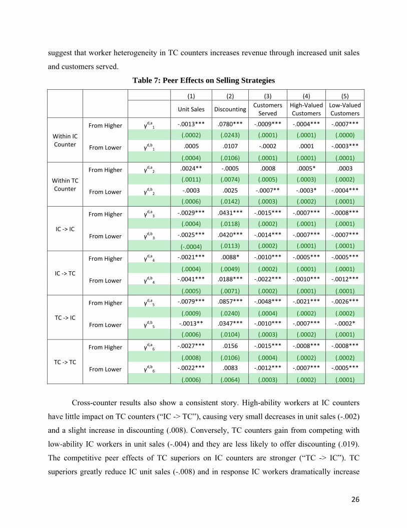
the asymmetric model in Table 7 (under columns 1 – 3).
The results illuminate the ways in which workers respond to peer effects. Increased
competition from improved outside peer quality lowers unit sales and the number of customers
served while increasing level of discounting. More importantly, the magnitude of these
estimated parameters depends strongly on the compensation system of both the focal worker and
her outside peer. Within IC counters, while superiors at the same counter hurt peer unit sales (-
.001) and customers served (-.0009), inferiors have little effect. As a response, workers change
their pricing strategy by offering discounts to potential customers. Column (2) shows that
superiors increase the price discounting of their peers (.078) while inferiors have no effect. These
results imply that worker heterogeneity in IC counters reduces revenue through reduced unit
sales and increased price discounting among workers with lower productivity. Results of peer
effects within TC counters tell a different story. While the existence of superior workers helps to
increase unit sales (.002), the existence of inferior workers increases the number of customers a
salesperson serves (-.007).14 There is no discounting effect within TC counters. All these results
14 The effect of the existence of superior workers on customers served, though positive, is insignificant.
25
suggest that worker heterogeneity in TC counters increases revenue through increased unit sales
and customers served.
Table 7: Peer Effects on Selling Strategies
(1) (2) (3) (4) (5) Customers Served
High‐Valued Customers
Low‐Valued Customers
Unit Sales Discounting
‐.0013*** .0780*** ‐.0009*** ‐.0004*** ‐.0007*** From Higher γd,a1 (.0002) (.0243) (.0001) (.0001) (.0000) Within IC
Counter .0005 .0107 ‐.0002 .0001 ‐.0003*** γd,b1 From Lower
(.0004) (.0106) (.0001) (.0001) (.0001)
.0024** ‐.0005 .0008 .0005* .0003 γd,a2 From Higher
(.0011) (.0074) (.0005) (.0003) (.0002) Within TC Counter ‐.0003 .0025 ‐.0007** ‐.0003* ‐.0004*** γd,b2
From Lower (.0006) (.0142) (.0003) (.0002) (.0001)
‐.0029*** .0431*** ‐.0015*** ‐.0007*** ‐.0008*** From Higher γd,a3
(.0004) (.0118) (.0002) (.0001) (.0001) IC ‐> IC
‐.0025*** .0420*** ‐.0014*** ‐.0007*** ‐.0007*** γd,b3 From Lower
(.0113) (.0002) (.0001) (.0001) (‐.0004)
‐.0021*** .0088* ‐.0010*** ‐.0005*** ‐.0005*** From Higher γd,a4
(.0004) (.0049) (.0002) (.0001) (.0001) IC ‐> TC
‐.0041*** .0188*** ‐.0022*** ‐.0010*** ‐.0012*** γd,b4 From Lower
(.0005) (.0071) (.0002) (.0001) (.0001)
‐.0079*** .0857*** ‐.0048*** ‐.0021*** ‐.0026*** From Higher γd,a5
(.0009) (.0240) (.0004) (.0002) (.0002) TC ‐> IC
‐.0013** .0347*** ‐.0010*** ‐.0007*** ‐.0002* γd,b5 From Lower
(.0006) (.0104) (.0003) (.0002) (.0001)
‐.0027*** .0156 ‐.0015*** ‐.0008*** ‐.0008*** γd,a6 From Higher
(.0008) (.0106) (.0004) (.0002) (.0002) TC ‐> TC
‐.0022*** .0083 ‐.0012*** ‐.0007*** ‐.0005*** γd,b6 From Lower
(.0006) (.0064) (.0003) (.0002) (.0001)
Cross-counter results also show a consistent story. High-ability workers at IC counters
have little impact on TC counters (“IC -> TC”), causing very small decreases in unit sales (-.002)
and a slight increase in discounting (.008). Conversely, TC counters gain from competing with
low-ability IC workers in unit sales (-.004) and they are less likely to offer discounting (.019).
The competitive peer effects of TC superiors on IC counters are stronger (“TC -> IC”). TC
superiors greatly reduce IC unit sales (-.008) and in response IC workers dramatically increase
26
discounting (.086). Yet IC counters gain very little from inferiors at TC competitors in terms of
unit sales (-.001) that is considerably less than the loss to TC superiors. The resistance of TC
counters to high-ability peers at competing counters is also evident in competition between TC
counters (“TC -> TC”). While we observe similar asymmetric peer effects, these are smaller
than those from TC counters to IC counters (“TC -> IC”). We also observe no peer effects
between TC counters in discounting. Collectively, these cross-counter peer effects suggest that
TC counters are better able to exploit weak workers at competing counters and defend
themselves from competitors’ star workers. This implies that coordination with team-based
counters, perhaps through specialization, creates better dynamic responses to variations in
worker-specific competition.
5.1 Peer Effects on Customer Mix
In response to the pressure from competing peers, a salesperson may employ strategies
other than price discounting. For example, she may exert different levels of effort toward serving
different types of customers. To investigate this possibility, we separate all the customers into
two groups, using the median dollars spending as the separating criterion. We label them high-
value (HV) customers and low-value (LV) customers. Columns (4) and (5) of Table 7 show the
results when we estimate model (5) using the number of customers in these two groups as
dependent variables.
Results again demonstrate negative peer effects within IC counters (γd1), but the level of
business stealing appears to be higher with LV customers (-.0007 vs. -.0004). Inferior coworkers
appear only lose LV customers to superiors within counter (-.0003). More importantly, our
results suggest some mechanisms through which worker heterogeneity might benefit TC
counters. Superiors increase coworker sales more than inferiors increase coworker sales to HV
customers (.0005 vs. -.0003), while only inferiors significantly increase coworker sales to LV
customers (-.0004). This suggests that workers at TC counters may coordinate in which
customers they serve: high-ability workers may let low-ability workers focus on selling to HV
customers while they focus on competing with other counters for casual walkthrough traffic who
are mainly LV customers. Since HV customers may purchase more units per transaction but may
be less numerous than the LV customers in the store, this result helps to explain our previous
findings that only high-ability workers help to increase unit sales for low-ability peers, and only
low-ability workers significantly help to increase customers served for high-ability workers.
27
Such a division of labor can be efficient if HV customers are brand-loyal and hence may
purchase from the counter regardless of who the salesperson is. But walk-through customers
must be competed for across counters, and assigning the best worker to this task may most
efficiently utilize the skill-set of the workers.15
6. Discussion and Conclusion
In this paper we find evidence of peer effects among retail cosmetic salespeople. The
peer effects are not simply productivity spillovers, as we also identify likely strategic responses
by workers to the ability of their peers. The direction and magnitude of these effects depend on
the compensation system used by the brand. When faced with high-ability peers within the
counter, workers under individual-based compensation employ two strategic responses. First,
they discount their prices offered to customers. Second, they focus on retaining high-value repeat
customers, who likely are more loyal to specific brands. Still, they will lose (especially low-
value) customers since they are unable to compete with high-ability peers in selling techniques.
However, high-ability workers do not gain much overall. The reason is that workers at IC
counters are less able to compete with outside peers especially from TC counters. Focusing on
competing against each other, workers at IC counters can only devote limited effort to outside
competition, and therefore are greatly impacted by high-ability outside peers. Our results
demonstrate how the relationship between worker heterogeneity and team performance depends
critically on compensation system – under individual-based compensation, heterogeneity can
lead to internal customer and price competition, and loss of sales to outside competition.
In contrast, larger heterogeneity enhances team performance under team-based
compensation. We find that high-ability workers significantly improve the sales productivity of
their peers. Workers appear to coordinate on which customers they serve: low-ability workers
may focus more on loyal high-value customers while high-ability workers compete for casual
walkthrough customers who are most difficult to gain. Workers at these counters, finding it
unnecessary to exert effort toward within-counter competition, can focus all effort toward
outside competitors. Consequently, these workers lose fewer customers to outside peers and
offer less discounting to customers, hence suffering less revenue loss. High-ability workers at 15 Interviews with the store management revealed that customer brand loyalty is very important for the cosmetics category. Once a customer is used to using a product, the cost of her switching to other products is very high. Therefore, the task of selling to a brand-loyal customer is much easier than attracting a new customer.
28
TC counters, on the other hand, have much larger negative effects on outside peers than do their
IC counter peers.
This paper is the first empirical study that simultaneously estimates peer effects within
and across firms under multiple compensation systems. It is also the first to identify some
strategies employed by workers in response to peer effects, and provides important implications
for managerial decisions on staffing, compensation, and pricing discretion. Our results are
consistent with existing theoretical models on incentives and employee helping behavior and task
choice. We hope that our rich findings of peer effects in co-located sales teams will provide
useful insights to stimulate future theoretical development, particularly in the context of cross-
firm competition. Previous research suggests that productivity spillovers may occur from
knowledge transfer, coordination and specialization, social pressure, and free-riding in teamwork.
Empirical studies suggest that diversity will increase gains in a team. Yet these studies do not
compare peer effects under different incentive schemes. We show that workers under individual-
based compensation system respond to high ability peers by price discounting and strategically
choosing customer types. Due to these behaviors, larger heterogeneity leads to lower team
performance, especially when outside competition exists. We believe theoretically explicating
how worker strategies under peer effects depend on compensation is important for future
research. Furthermore, to our best knowledge, there has been no research in labor economics on
how compensation system may influence the capability of a team or firm to compete against
other teams or firms. Some of the existing theories on firm competition from the IO and strategy
literature may be useful in addressing this issue. Our results on how peer effects spill across firm
boundaries and instigate strategic responses from peers within and across firms may provide
useful insights for future studies.
Finally, we note that there are several other issues in our analysis that should be
addressed. First, we are unable to compare workers’ overall productivity under individual-based
and team-based compensation system. To achieve this would require counters to change their
compensation systems in the data. Second, while we have identified the contemporary peer
effects within and across counters, our model abstracts away from long-term peer effects that
may be resulted from peer learning through team coordination or competition. A dynamic model
allowing for peer learning can help to investigate this long-term effect. Addressing these two
29

issues will allow us to finally study under what conditions it will be optimal for firms in a
competition environment to adopt individual-based vs. team-based compensation system.
30
References Asch, Beth J. 1990. “Do Incentives Matter? The Case of Navy Recruiters.” Industrial and Labor
Relations Review, Vol. 43, No. 3, pp. 89S-106S. Baker, George P., Robert Gibbons, and Kevin J. Murphy. 1994. “Subjective Performance
Measures in Optimal Incentive Contracts.” Quarterly Journal of Economics, Vol. 109, No. 4 (Nov., 1994), pp. 1125-1156.
Baker, George P. 1992. “Incentive Measures and Performance Measurement.” Journal of Political Economy, Vol. 100, No. 3 (Jun., 1992), pp. 598-614.
Bandiera, Oriana, Iwan Barankay, and Imran Rasul. Forthcoming. “Social Connections and Incentives in the Workplace: Evidence from Personnel Data.” Econometrica.
Berg, Perter, Eileen Appelbaum, Thomas Bailey, and Arne L. Kalleberg. 1996. “The Performance Effects of Modular Production in the Apparel Industry.” Industrial Relations, Vol. 35, Issue 3 (Jul., 1996), pp. 356-373.
Bernheim, Douglas B. 1994. “A Theory of Conformity.” Journal of Political Economy, Vol. 102, No. 5 (Oct., 1994), pp. 841-877.
Boning, Brent, Casey Ichniowski, and Kathryn Shaw. 2007. “Opportunity Counts: Teams and the Effectiveness of Production Incentives.” Journal of Labor Economics, Vol. 25, No. 4, pp. 613-650.
Che, Yeon-Koo, and Seung-Weon Yoo. 2001. “Optimal Incentives for Teams.” The American Economic Review, Vol. 91, No. 3 (Jun., 2001), pp. 525-541.
Courty, Pascal, and Gerald Marschke. 2004. ”An Empirical Investigation of Gaming Responses to Explicit Performance Incentives.” Journal of Labor Economics, Vol. 22, No. 1, pp. 23-56.
Falk, Armin, and Andrea Ichino. 2006. “Clean Evidence on Peer Effects.” Journal of Labor Economics, Vol. 24, No. 1, pp. 39-57.
Gant, Jon, Casey Ichniowski, and Kathryn Shaw. 2002. “Social Capital and Organizational Change in High-Involvement and Traditional Work Organizations.” Journal of Economics &Management Strategy, Vol. 11, Issue 2, pp. 289-328.
Gant, Jon, Casey Ichniowski, and Kathryn Shaw. 2003. "Working Smarter by Working Together: Connective Capital in the Workplace." http://client.norc.org/jole/SOLEweb/shaw.pdf.
Guryan, Jonathan, Matt Notowidigdo, and Kory Kroft. Forthcoming. “Peer Effects in the Workplace: Evidence from Random Groupings in Professional Golf Tournaments.” American Economic Journal: Applied Economics.
Hamilton, Barton H., Jack A. Nickerson, and Hideo Owan. 2003. “Team Incentives and Worker Heterogeneity: An Empirical Analysis of the Impact of Teams on Productivity and Participation.” Journal of Political Economy, Vol. 111, No 3, pp. 465-497.
Holländer, Heinz. 1990. “A Social Exchange Approach to Voluntary Cooperation.” The American Economic Review, Vol. 80, No. 5 (Dec., 1990), pp. 1157-1167.
Holmstrom, Bengt. 1979. “Moral Hazard and Observability.” The Bell Journal of Economics, Vol. 10, No. 1 (Spring, 1979), pp. 74-91.
Holmstrom, Bengt. 1982. “Moral Hazard in Teams.” The Bell Journal of Economics, Vol. 13, No. 2 (Autumn, 1982), pp. 324-340.
Holmstrom, Bengt, and Paul Milgrom. 1991. “Multitask Principal-Agent Analyses: Incentive Contracts, Asset Ownership, and Job Design.” Journal of Law, Economics, and
31
32
Organization, Vol. 7, Special Issue: [Papers from the Conference on the New Science of Organization, January 1991] (1991), pp. 24-52.
Holmstrom, Bengt, and Paul Milgrom. 1994. “The Firm as an Incentive System.” The American Economic Review, Vol. 84, No. 4 (Sep., 1994), pp. 972-991.
Ichino, Andrea, and Giovanni Maggi. 2000. “Work Environment And Individual Background: Explaining Regional Shirking Differentials In A Large Italian Firm.” Quarterly Journal of Economics, Vol. 115, No. 3 (Aug., 2000), Pages 1057-1090.
Itoh, Hideshi. 1991. “Incentives to Help in Multi-Agent Situations.” Econometrica, Vol. 59, No. 3 (May, 1991), pp. 611-636.
Itoh, Hideshi. 1992. “Cooperation in Hierarchical Organizations: An Incentive Perspective.” Journal of Law, Economics, and Organization, 8(2), 321-345.
Itoh, Hideshi. 1993. “Coalitions, Incentives, and Risk Sharing.” Journal of Economic Theory, 60, 410-427.
Kandel, Eugene, and Edward P. Lazear. 1992. “Peer Pressure and Partnerships.” Journal of Political Economy, Vol. 100, No.4, pp. 801-817.
Larkin, Ian, 2008. “The Cost of High-Powered Incentives: Employee Gaming in Enterprise Software Sales.” http://isites.harvard.edu/fs/docs/icb.topic443134.files/LARKIN_12-11.pdf.
Lazear, Edward P., and Sherwin Rosen. 1981. “Rank-Order Tournaments as Optimum Labor Contracts.” Journal of Political Economy, Vol. 89, No. 5 (Oct., 1981), pp. 841-864.
Lazear, Edward P. 1989. “Pay Equality and Industrial Politics.” Journal of Political Economy, Vol. 97, No. 3 (Jun., 1989), pp. 561-580.
Lazear, Edward P. 2000. “Performance Pay and Productivity.” The American Economic Review, Vol. 90, No. 5 (Dec., 2000), pp. 1346-1361.
Leonard, Jonathan, and David Levine. 2006. “The Effect of Diversity on Turnover: Evidence from a Very Large Case Study.” Industrial Relations and Labor Review, Vol. 59, No. 4 (Jul., 2006), pp. 547-572.
Lucas, Robert E. 1988. “On the mechanics of economic development.” Journal of Monetary Economics, 22, 3–42.
MacDonald, Glenn, and Leslie M. Marx. 2001. “Adverse Specialization.” Journal of Political Economy, Vol. 109, No 4, pp. 864-899.
Marshall, Alfred. 1890. The Principles of Economics, London: MacMillan. Mas, Alexandre, and Enrico Moretti. 2009. “Peers at Work.” The American Economic Review,
Vol. 99, No. 1 (Mar., 2009), pp. 112-145. Neler, J. A., and R. Mead. 1965. “A Simplex Method for Function Minimization.” Computer
Journal, 7, 308-313. Oyer, Paul. 1998. “Fiscal Year Ends and Non-Linear Incentive Contracts: The Effect on
Business Seasonality.” Quarterly Journal of Economics, Vol. 113, No. 1, pp. 149-185. Pierce, Lamar, and Jason Snyder. 2008. “Ethical Spillovers in Firms: Evidence from Vehicle
Emissions Testing.” Management Science, 54(11), 1891-1903.